to the university of wyoming: 4/18/2012. jeffrey l. beck, ph.d ... · dr. jeff beck, for providing...
TRANSCRIPT

To the University of Wyoming:
The members of the Committee approve the thesis of Chad W. LeBeau presented on
4/18/2012.
Jeffrey L. Beck, Ph.D., Chairperson
Kenneth Gerow, Ph.D., External Department Member
Matthew J. Holloran, Ph.D.
Gregory D. Johnson
Scott N. Miller, Ph.D.
APPROVED:
John A. Tanaka, Head, Department of Ecosystem Science and Management
Francis D. Galey, Dean, College of Agriculture and Natural Resources
1
LeBeau, Chad, W, Evaluation of Greater Sage-Grouse Reproductive Habitat and Response to
Wind Energy Development in South-Central, Wyoming, MS, Department of
Ecosystem Science and Management, August 2012.
The demand for clean renewable energies and tax incentives has prompted a nationwide
increase in wind energy development. Renewable energy development is occurring in a wide
variety of habitats potentially impacting many species including greater sage-grouse
(Centrocercus urophasianus). Greater sage-grouse require contiguous intact sagebrush
(Artemisia spp.) habitats. The addition of wind energy infrastructure to these landscapes may
negatively impact population viability. Greater sage-grouse are experiencing range-wide
population declines and are currently listed as a candidate species under the Endangered Species
Act of 1973. The purpose of my study was to investigate the response of greater sage-grouse to
wind energy development. Mine is the first study to document the short-term effects of wind
energy infrastructure on greater sage-grouse habitat selection, nest, brood, and female survival,
and male lek attendance. I hypothesized that greater sage-grouse would select for habitats farther
from wind energy infrastructure, particularly wind turbines, during the nesting, brood-rearing,
and summer periods. In addition, I hypothesized that greater sage-grouse nest, brood, and female
survival would decline in habitats with close proximity to wind turbines. Lastly, I hypothesized
that greater sage-grouse male lek attendance would experience greater declines from pre wind
energy development to 4 years post development at leks with close proximity to wind turbines
compared to leks farther from turbines.
My study area was located in south-central Wyoming between the towns of Medicine
Bow and Hanna and consisted of one study area influenced by wind energy development (Seven

2
Mile Hill) and a second study area that was not impacted by wind energy development (Simpson
Ridge). I identified 14 leks within both study areas and conducted lek counts at each of these leks
from 2008 to 2012. I captured 116 female greater sage-grouse from both study areas from 2009
to 2010. I equipped each female grouse with a VHF necklace-mounted transmitter and monitored
them via telemetry during the nesting, brood-rearing, and summer periods within both study
areas from 2009 to 2010. I documented greater sage-grouse habitat selection as well as nest and
brood-rearing success and female survival. I used binary logistic regression in a use versus
availability study design to estimate the odds of habitat selection within both study areas during
the nesting, brood-rearing, and summer periods. I used Cox proportional hazards and Andersen-
Gill survival models to estimate nest, brood, and female survival relative to wind energy
infrastructure. Lastly, I used ratio of means tests and linear mixed effects models to estimate the
degree of decline in male lek attendance at leks influenced by wind energy development versus
leks with no influence 1 year prior to development to 4 years post development.
Greater sage-grouse did not avoid wind turbines during the nesting and brood-rearing
periods, but did select for habitats closer to turbines during the summer season. Greater sage-
grouse nest and brood survival decreased in habitats in close proximity to wind turbines, whereas
female survival appeared not to be affected by wind turbines. Peak male lek attendance within
both study areas experienced significant declines from 1 year pre development to 4 years post
development; however, this decline was not attributed to the presence of the wind energy facility.
The results from my study are the first examining the short-term impacts to greater sage-
grouse populations from wind energy development. Greater sage-grouse were not avoiding the
wind energy development two years following construction and operation of the wind energy
facility. This is likely related to high site fidelity inherent in sage-grouse. In addition, more

3
suitable habitat may exist closer to turbines at Seven Mile Hill, which may also be driving
selection. Fitness parameters including nest and brood survival were reduced in habitats of close
proximity to wind turbines and may be the result of increased predation and edge effects
associated with the wind energy facility. Lastly, wind energy infrastructure appears not to be
affecting male lek attendance 4 years post development; however, time lags are characteristic in
greater sage-grouse populations, which may result in impacts not being quantified until 2–10
years following development. Future wind energy developments should identify greater sage-
grouse nest and brood-rearing habitats prior to project development to account for the decreased
survival in habitats of close proximity to wind turbines. More than 2 years of occurrence data
and more than 4 years of male lek attendance data may be necessary to account for the strong site
fidelity and time lags present in greater sage-grouse populations.

EVALUATION OF GREATER SAGE-GROUSE REPRODUCTIVE HABITAT AND
RESPONSE TO WIND ENERGY DEVELOPMENT IN SOUTH-CENTRAL, WYOMING
By
Chad W. LeBeau
A thesis submitted to the Department of Ecosystem Science and Management
and the University of Wyoming
in partial fulfillment of the requirements
for the degree of
MASTER OF SCIENCE
in
RANGELAND ECOLOGY AND WATERSHED MANAGEMENT
Laramie, Wyoming
August 2012

ii
COPYRIGHT PAGE
Copyright 2012, Chad W. LeBeau

iii
ACKNOWLEDGMENTS
The initial portion of my study was primarily funded by the wind energy industry, with EDP
Renewable (formerly Horizon Wind Energy) being the principal source of funding. Iberdrola
Renewables contributed funding for radio-telemetry collars, and the Shirley Basin/Bates Hole
Local Sage-Grouse Working Group provided funding for relocation flights. I thank the United
States Department of Energy for providing a substantial grant that assisted in funding my study.
The University of Wyoming School of Energy Resources and EDP Renewables provided tuition
and fees for my graduate studies at the University of Wyoming. I thank Greg Johnson of Western
EcoSystems Technology, Inc. and Matt Holloran of Wyoming Wildlife Consultants, LLC for
providing access to the data for this study. I thank Ryan Nielson of Western EcoSystems
Technology, Inc. for providing valuable input to statistical procedures used in my thesis. I thank
PacifiCorp for allowing access to the Seven Mile Hill Wind Energy Facility for study purposes. I
especially thank Burt and Kay Lynn Palm for providing access to their private land. I thank
Christopher Kirol for his valuable input on study design used in my study. I thank my advisor
Dr. Jeff Beck, for providing me with this opportunity, obtaining funding for my graduate
support, and guiding me through my study. In addition, I thank my committee members, Dr. Jeff
Beck, Dr. Scott Miller, and Dr. Ken Gerow with the University of Wyoming, Greg Johnson of
Western EcoSystems Technology, Inc., and Dr. Matt Holloran of Wyoming Wildlife
Consultants, LLC. I appreciate the assistance of Troy Rintz, Jason Herreman, and Victoria
Poulton who helped capture sage-grouse. Jamey Eddy, Greg Leighty, Jason Herreman, Ariana
Malone, and Brandon Smith assisted with relocating radio-marked sage-grouse and conducting
lek counts; all of whom were valuable contributors to my study. Lastly, I would like to thank my
wife Rachel for all her support.
iv
TABLE OF CONTENTS
ACKNOWLEDGMENTS ............................................................................................................. iii
LIST OF TABLES ........................................................................................................................ vii
LIST OF FIGURES ........................................................................................................................ x
CHAPTER 1 Introduction............................................................................................................... 1
WIND ENERGY DEVELOPMENT ........................................................................... 1
GREATER SAGE-GROUSE POPULATION TRENDS .......................................... 3
STUDY PURPOSE ....................................................................................................... 4
STUDY AREA ............................................................................................................... 5
LITERATURE CITED ................................................................................................ 7
CHAPTER 2 Greater Sage-Grouse Habitat Selection Relative to Wind Energy Infrastructure in
South-Central, Wyoming.................................................................................................... 13
ABSTRACT ................................................................................................................. 13
INTRODUCTION....................................................................................................... 14
STUDY AREA ............................................................................................................. 15
METHODS .................................................................................................................. 16
Field Methods ........................................................................................................... 17
GIS Covariates .......................................................................................................... 19
Model development ................................................................................................... 20
RESULTS .................................................................................................................... 24
Nest Site Selection ..................................................................................................... 25
Brood-rearing Habitat Selection .............................................................................. 26
Summer Habitat Selection......................................................................................... 28

v
DISCUSSION .............................................................................................................. 29
Nest Site Selection ..................................................................................................... 31
Brood-rearing Habitat selection ............................................................................... 32
Summer Habitat Selection......................................................................................... 33
MANAGEMENT IMPLICATIONS ......................................................................... 35
LITERATURE CITED .............................................................................................. 36
CHAPTER 3 Greater Sage-grouse Fitness Parameters Associated with Wind Energy
Development ...................................................................................................................... 61
ABSTRACT ................................................................................................................. 61
INTRODUCTION....................................................................................................... 62
STUDY AREA ............................................................................................................. 65
METHODS .................................................................................................................. 65
Field Methods ........................................................................................................... 65
GIS Covariates .......................................................................................................... 67
Survival Parameters.................................................................................................. 68
Model Development .................................................................................................. 70
RESULTS .................................................................................................................... 73
Nest Survival ............................................................................................................. 73
Brood Survival .......................................................................................................... 75
Female Survival ........................................................................................................ 77
DISCUSSION .............................................................................................................. 79
MANAGEMENT IMPLICATIONS ......................................................................... 82
LITERATURE CITED .............................................................................................. 83

vi
CHAPTER 4 Greater Sage-Grouse Male Lek Attendance Relative to Wind Energy Development
.......................................................................................................................................... 101
ABSTRACT ............................................................................................................... 101
INTRODUCTION..................................................................................................... 102
STUDY AREA ........................................................................................................... 103
METHODS ................................................................................................................ 103
Field Methods ......................................................................................................... 103
Analytical Methods ................................................................................................. 105
RESULTS .................................................................................................................. 108
Model Development ................................................................................................ 109
DISCUSSION ............................................................................................................ 110
LITERATURE CITED ............................................................................................ 112
vii
LIST OF TABLES
Table 2-1. Explanatory anthropogenic and environmental covariates used in model selection for
sage-grouse nest site, brood-rearing, and summer habitat selection at the Seven Mile Hill
and Simpson Ridge study areas, Carbon County Wyoming, USA, 2009 and 2010 (Homer
et al. 2012). ....................................................................................................................... 42
Table 2-2. Model fit statistics for greater sage-grouse nest site selection at the Seven Mile Hill
and Simpson Ridge study areas, Carbon County, Wyoming, USA, 2009 and 2010.
Models are listed according to the model best fitting the data and ranked by (ΔAICc), the
difference between the model with the lowest Akaike’s Information Criterion for small
samples (AICc) and the AICc for the current model. The value of the maximized log-
likelihood function (log[L]), the number of estimated parameters (K), and Akaike’s
weights (wi) for each model are also presented. ............................................................... 43
Table 2-3. Odds ratios, slope coefficients, and 90% confidence intervals (CI) in the sage-grouse
top nest site selection model for the Seven Mile Hill and Simpson Ridge study areas in
Carbon County, Wyoming, USA, 2009 and 2010. Odds ratios measure the multiplicative
change in odds of selection when a covariate changes by 1 unit, assuming all other
covariates remain constant. ............................................................................................... 44
Table 2-4. Model fit statistics for greater sage-grouse brood selection at the Seven Mile Hill and
Simpson Ridge study areas, Carbon County, Wyoming, USA, 2009 and 2010. Models are
listed according to the model best fitting the data and ranked by (ΔAICc), the difference
between the model with the lowest Akaike’s Information Criterion for small samples
(AICc) and the AICc for the current model. The value of the maximized log-likelihood

viii
function (log[L]), the number of estimated parameters (K), and Akaike’s weights (wi) for
each model are also presented........................................................................................... 45
Table 2-5. Odds ratios, slope coefficients, and 90% confidence intervals (CI) for covariates in the
sage-grouse top brood-rearing selection model for the Seven Mile Hill and Simpson
Ridge study areas in Carbon County, Wyoming, USA, 2009 and 2010. Odds ratios
measure the multiplicative change in odds of selection when a covariate changes by 1
unit, assuming all other covariates remain constant. Odds ratios were not calculated for
covariates involved with a quadratic effect because they were dependent on values of
other covariates. ................................................................................................................ 46
Table 2-6. Model fit statistics for greater sage-grouse summer selection at the Seven Mile Hill
and Simpson Ridge study areas, Carbon County, Wyoming, USA, 2009 and 2010.
Models are listed according to the model best fitting the data and ranked by (ΔAICc), the
difference between the model with the lowest Akaike’s Information Criterion for small
samples (AICc) and the AICc for the current model. The value of the maximized log-
likelihood function (log[L]), the number of estimated parameters (K), and Akaike’s
weights (wi) for each model are also presented. ............................................................... 47
Table 2-7. Odds ratios, slope coefficients, and 90% confidence intervals (CI) for covariates in the
sage-grouse top summer selection model for the Seven Mile Hill and Simpson Ridge
study areas in Carbon County, Wyoming, USA, 2009 and 2010. Odds ratios measure the
multiplicative change in odds of selection when a covariate changes by 1 unit, assuming
all other covariates remain constant. Odds ratios were not calculated for covariates
involved with a quadratic effect because they were dependent on values of other
covariates. ......................................................................................................................... 48

ix
Table 3-1. Explanatory anthropogenic and environmental covariates used in modeling of sage-
grouse nest, brood, and female survival at the Seven Mile Hill and Simpson Ridge study
areas, Carbon County Wyoming, USA, 2009 and 2010. .................................................. 91
Table 3-2. Model fit statistics for greater sage-grouse nest, brood, and survival at the Seven Mile
Hill and Simpson Ridge study areas, Carbon County, Wyoming, USA, 2009 and 2010.
Models are listed according to the model best fitting the data and ranked by (Δ AICc), the
difference between the model with the lowest Akaike’s Information Criterion for small
samples (AICc) and the AICc for the current model. The value of the maximized log-
likelihood function (log[L]), the number of estimated parameters (K), and Akaike’s
weights (wi) for each model are also presented. ............................................................... 92
Table 3-3. Relative risks of sage-grouse for each covariate or risk factor included in the top
model for the Seven Mile Hill and Simpson Ridge study areas in Carbon County,
Wyoming, USA, 2009 and 2010. ...................................................................................... 93
Table 4-1. Disturbance metrics included in the mixed modeling procedure to determine potential
extents of impact from turbines to male lek attendance at leks located within the Seven
Mile Hill and Simpson Ridge study areas in Carbon County Wyoming, USA, 2008–2012.
Metrics were derived from male breeding use areas (0.60 km), identified management
areas (3.2 km), or disturbance distances previously determined from oil and gas
development. ................................................................................................................... 116
Table 4-2. Maximum counts, yearly averages, and totals of male sage-grouse on occupied leks
located within the Seven Mile Hill and Simpson Ridge study areas, Carbon County,
Wyoming, USA, 2008–2012. Entries of “NA” indicate no count was conducted. ........ 117

x
LIST OF FIGURES
Figure 1-1. Seven Mile Hill and Simpson Ridge study areas located in Carbon County,
Wyoming, USA. The Seven Mile Hill Wind Energy facility consisted of 79, 1.5-MW
wind turbines. The Simpson Ridge study area comprised of the area within and
surrounding the Simpson Ridge Wind Resource Area (SRWRA). .................................. 12
Figure 2-1. Odds ratios or relative probability of sage-grouse nest site selection and 90%
confidence intervals (dashed lines) within the Seven Mile Hill study area as a function of
top model covariates, Carbon County, Wyoming, USA, 2009 and 2010. All other
covariates in the best approximating model were held constant at their mean value.
Overlapping confidence limits indicate a non-significant estimate. ................................. 49
Figure 2-2. Odds ratios or relative probability of sage-grouse nest site occurrence and 90%
confidence intervals (dashed lines) within the Simpson Ridge study area as a function of
top model covariates, Carbon County, Wyoming, USA, 2009 and 2010. All other
covariates in the best approximating model were held constant at their mean value. ...... 50
Figure 2-3. Predicted nesting habitat used within a 129 km2 minimum convex polygon by sage-
grouse within the Seven Mile Hill study area, Carbon County, Wyoming, USA, 2009 and
2010................................................................................................................................... 51
Figure 2-4. Predicted nesting habitat used within a 217 km2 minimum convex polygon by sage-
grouse within the Simpson Ridge Study area, Carbon County, Wyoming, USA, 2009 and
2010................................................................................................................................... 52
Figure 2-5. Odds ratios or relative probability of sage-grouse brood-rearing selection and 90%
confidence intervals (dashed lines) within the Seven Mile Hill study area as a function of
top model covariates, Carbon County, Wyoming, USA, 2009 and 2010. Confidence

xi
intervals were not calculated for distance to transmission line because confidence
intervals for quadratic effects depend on values of other covariates. ............................... 53
Figure 2-6. Odds ratios or relative probability of sage-grouse brood-rearing occurrence and 90%
confidence intervals (dashed lines) within the Simpson Ridge study area as a function of
top model covariates, Carbon County, Wyoming, USA, 2009 and 2010. All other
covariates in the best approximating model were held constant at their mean value.
Overlapping confidence limits indicate a non-significant estimate. ................................. 54
Figure 2-7. Predicted brood-rearing habitat used within a 126 km2 minimum convex polygon by
sage-grouse within the Seven Mile Hill study area, Carbon County, Wyoming, USA,
2009 and 2010. .................................................................................................................. 55
Figure 2-8. Predicted brood-rearing habitat used within a 650 km2 minimum convex polygon by
sage-grouse within the Simpson Ridge study area, Carbon County, Wyoming, USA, 2009
and 2010. ........................................................................................................................... 56
Figure 2-9. Odds ratios or relative probability of female sage-grouse summer occurrence and
90% confidence intervals (dashed lines) within the Seven Mile Hill study area as a
function of top model covariates, Carbon County, Wyoming, USA, 2009 and 2010. All
other covariates in the best approximating model were held constant at their mean value.
........................................................................................................................................... 57
Figure 2-10. Odds ratios or relative probability of female sage-grouse summer occurrence and
90% confidence intervals (dashed lines) within the Simpson Ridge study area as a
function of top model covariates, Carbon County, Wyoming, USA, 2009 and 2010. All
other covariates in the best approximating model were held constant at their mean value.
xii
Confidence intervals were not calculated for distance to major road because confidence
intervals for quadratic effects depend on values of other covariates. ............................... 58
Figure 2-11. Predicted summer habitat used within a 243 km2 minimum convex polygon by
sage-grouse within the Seven Mile Hill study area, Carbon County, Wyoming, USA,
2009 and 2010. .................................................................................................................. 59
Figure 2-12. Predicted summer habitat used within a 751 km2 minimum convex polygon by
sage-grouse within the Simpson Ridge study area, Carbon County, Wyoming, USA, 2009
and 2010. ........................................................................................................................... 60
Figure 3-1. Relative hazard rate of nest survival adjusted for the SD of shrub height within 0.30
km, and the distance to nearest turbine and transmission line at the Simpson Ridge and
Seven Mile Hill study areas, Carbon County, Wyoming, USA, 2009 and 2010. Dashed
lines indicate the lower and upper 90% confidence limits. .............................................. 94
Figure 3-2. Expected nest survival and 90% confidence intervals for nests located in higher risk
habitats (closer to turbines, further from transmission lines, and higher SD of shrub
height within 0.30 km; poor nest survival) and for nests located in lower risk habitats
(good nest survival) within the Simpson Ridge and Seven Mile Hill study areas Carbon
County, Wyoming, USA, 2009 and 2010. ........................................................................ 95
Figure 3-3. Spatial variation in the predicted relative risk of sage-grouse nest failure (low – high)
within the Seven Mile Hill and Simpson Ridge study areas, Carbon County, Wyoming,
USA, 2009 and 2010. ........................................................................................................ 96
Figure 3-4. Relative hazard rate of brood survival adjusted for distance to nearest turbine, terrain
ruggedness, and percent shrub cover at the Simpson Ridge and Seven Mile Hill study

xiii
areas, Carbon County, Wyoming, USA, 2009 and 2010. Dashed lines indicate the lower
and upper 90% confidence limits. ..................................................................................... 97
Figure 3-5. Spatial variation in the predicted relative risk of sage-grouse brood failure (low –
high) within the Seven Mile Hill and Simpson Ridge study areas, Carbon County,
Wyoming, USA, 2009 and 2010. ...................................................................................... 98
Figure 3-6. Relative hazard rate of female survival adjusted for the distance to nearest major road
and distance to nearest overhead transmission line at the Simpson Ridge and Seven Mile
Hill study areas, Carbon County, Wyoming, USA, 2009 and 2010. Dashed lines indicate
the lower and upper 90% confidence limits. ..................................................................... 99
Figure 3-7. Spatial variation in the predicted relative risk of sage-grouse summer mortality (low
– high) within the Seven Mile Hill and Simpson Ridge study areas, Carbon County,
Wyoming, USA, 2009 and 2010. .................................................................................... 100
Figure 4-1. Lek locations within the Seven Mile Hill and Simpson Ridge study areas located in
Carbon County, Wyoming, USA, 2008–2011. ............................................................... 118
Figure 4-2. Ratio of means (± 90% CI) of peak male lek attendance observed at Simpson Ridge
(SR), Seven Mile Hill (SMH), and regional (REG) leks from 2008–2012, Carbon County
Wyoming, USA. Pre-development (2008) counts were used as the baseline to detect
changes in peak male lek attendance to 4 years post development. The 2012 lek data was
not available for the regional lek population at time of publication. .............................. 119
Figure 4-3. The distribution of standardized residuals from the linear regression model
comparing male lek attendance to year and study area in Carbon County, Wyoming,
USA, 2008–2012. The standardized residuals were plotted against individual leks within
both study areas. Leks located above and below the zero residual line indicate within lek

xiv
correlation. Boxes include the interquartile range (25th–75th percentile) in standardized
residuals; horizontal lines inside boxes are median standardized residuals; lower and
upper whiskers are standardized residuals extending to 1.5 times the interquartile range.
......................................................................................................................................... 120

1
CHAPTER 1
Introduction
WIND ENERGY DEVELOPMENT
Increasing concern for environmental sustainability and the demand for domestic energy have
led to investment in renewable energies including biofuels, geothermal, hydropower, solar, and
wind in the United States. The United States has adopted a nationwide energy policy focused on
renewable energies that states that 20% of all electricity will be provided by wind energy by
2030 (DOE 2008). This initiative has triggered a nationwide increase in wind energy
development. In addition, energy demand and tax incentives are encouraging prolific
development of wind energy resources, making wind energy the fastest growing renewable
energy source.
Wind energy development is occurring across many different landscapes, potentially
resulting in habitat fragmentation for numerous wildlife species, ultimately leading to indirect
and direct impacts (Kuvlesky et al. 2007). Direct impacts to wildlife species include bird and bat
collisions with wind turbine blades or other infrastructure associated with wind energy
development (e.g., guy wires, meteorological towers, and power lines). Such impacts to birds
and bats are well documented (e.g., Erickson et al. 2001, Johnson et al. 2003). While direct
impacts of wind energy development to birds and bats have been well documented, knowledge
of indirect impacts is lacking. Indirect impacts potentially resulting from size, noise, and
placement of turbines and associated wind energy infrastructure, including roads, transmission
lines, and power transfer stations, pose the greatest threat to wildlife (Kuvlesky et al. 2007). The
cumulative direct and indirect impacts from wind energy development to wildlife and their

2
habitats may contribute to overall declines in productivity and population persistence (WGFD
2009).
Wind energy development is increasing in prairie habitats with high wind capacity
(AWEA 2010). This has raised concerns over impacts to prairie grouse species including greater
sage-grouse (Centrocercus urophasianus), sharp-tailed grouse (Tympanuchus phasianellus), and
lesser (T. pallidicinctus), and greater (T. cupido) prairie-chickens (Kuvlesky et al. 2007).
Although direct impacts to prairie grouse are likely to be low, indirect impacts from
anthropogenic features are likely to occur (Kuvlesky et al. 2007). Pruett et al. (2009a) suggest
that indirect impacts of wind turbines and associated power transmission lines are likely to
impact prairie grouse movement because the species avoid tall structures and areas with human
activities. Pruett et al. (2009b) determined that lesser and greater prairie-chickens avoided
transmission lines and some major roads by at least 100 m in Oklahoma. There few publicly
available studies examining the response of prairie grouse species to wind energy development
(Johnson and Stephens 2010). Near an operating wind energy facility in Nebraska, prairie-
chicken and sharp-tailed grouse lek attendance appeared to be within the range of other non-
impacted leks during a 4-yr period (NGPC 2009). In Minnesota, nesting female prairie chickens
did not avoid wind turbines when selecting of adequate nesting habitat (Toepfer and Vodehnal
2009). Lastly, black grouse (Lyrurus tetrix) lek attendance was negatively impacted by wind
turbines 4-yrs after development of a facility in Austria (Zeiler and Grunschachner-Berger 2009).
Little information exists on the impacts of wind energy development on greater sage-
grouse (hereafter sage-grouse). However, numerous studies indicate that sage-grouse are
influenced by anthropogenic features including energy development (Lyon and Anderson 2003,
Holloran 2005, Doherty et al. 2008, Holloran et al. 2010). In addition, the degree of influence
3
varies by proximity to these features (Holloran 2005, Aldridge and Boyce 2007, Holloran et al.
2010). Holloran (2005) reported that adult female sage-grouse remained in traditional nesting
areas regardless of increasing development levels, though yearling females avoided energy
infrastructure by nesting farther away from development. Furthermore, Holloran et al. (2010)
determined the number of yearling female nests within 950 m of infrastructure was less than
expected and the number of nests outside of 950 m was more than expected. Holloran (2005)
found that sage-grouse nests were more successful in areas of lower natural gas well densities,
compared to that of higher density areas. In addition, nest initiation rates were reduced in areas
of greater vehicle traffic from gas development (Lyon and Anderson 2003).
Similar to nesting parameters, impacts from anthropogenic features also influence brood-
rearing parameters. Aldridge and Boyce (2007) reported that chick mortality was 1.5-times
higher in habitats where oil and gas wells were visible 1 km from brood-rearing sites. Lastly,
male sage-grouse lek attendance rates have been negatively impacted by oil and gas development
(Holloran 2005, Walker et al. 2007, Doherty 2008, Harju et al. 2010).
These examples describe some degree of influence by anthropogenic features on sage-
grouse distribution and productivity (Holloran 2005, Aldridge and Boyce 2007, Holloran et al.
2010). However, studies addressing the potential impacts of wind energy development to prairie
grouse, especially sage-grouse, are lacking.
GREATER SAGE-GROUSE POPULATION TRENDS
Sage-grouse occur in Alberta, California, Colorado, Idaho, Montana, Nevada, North Dakota,
Oregon, Saskatchewan, South Dakota, Utah, Washington, and Wyoming, where they occupy
about 56% of their historical pre-settlement range (Schroeder et al. 2004). Sage-grouse have
been experiencing range-wide population declines, and many monitored populations have been

4
declining 2% per year since 1965 (Connelly et al. 2004). Garton et al. (2011) predicted that at
least 13% of sage-grouse populations may decline below effective population sizes of 500 within
the next 30 years. Also, Garton et al. (2011) projected that 75% of populations and 29% of the 7
management zones in the United States are likely to decline below effective population sizes of
500 within 100 yrs if current conditions and trends persist.
The decline in sage-grouse populations has been attributed to degradation of sagebrush
habitats (Knick et al. 2003, Connelly et al. 2004, and Aldridge et al. 2008) from disturbance
factors including agricultural conversion (Swenson et al. 1987, Connelly et al. 2004), invasions
of exotic plants leading to increased fire frequencies (Knick et al. 2003, Connelly et al. 2004),
and more recently energy exploitation and extraction (Lyon and Anderson 2003, Holloran 2005,
Holloran et al. 2010, Doherty et al. 2011, Naugle et al. 2011). Sage-grouse are a sagebrush
obligate species (Braun et al. 1977), entirely dependent on healthy continuous sagebrush habitats
for successful reproduction and survival (Schroeder et al. 1999, Connelly et al. 2004).
Fragmentation and degradation of these sagebrush habitats inhibit sage-grouse productivity and
survival, which have long-term impacts on affected sage-grouse populations. Understanding the
current threats and potential new threats to the viability of sage-grouse populations is imperative
to the conservation of this species.
STUDY PURPOSE
The conservation efforts of sage-grouse populations must consider all potential threats that
inhibit population viability. Energy exploitation that includes oil and gas development is
considered a threat to sage-grouse population viability (Lyon and Anderson 2003, Holloran
2005, Holloran et al. 2010, Doherty et al. 2011, Naugle et al. 2011). Energy exploitation in the
form of wind energy may pose similar threats to sage-grouse populations; however, the extent of
5
these impacts on population viability is unknown. My study was the first study examining the
potential short-term impacts to sage-grouse populations from wind energy development. The
purpose of my study was to estimate the effects of wind energy infrastructure, particularly wind
turbines, on sage-grouse habitat selection patterns, population demographics, and male lek
attendance.
STUDY AREA
My study area was located in Carbon County, Wyoming between the towns of Medicine Bow
and Hanna (Fig. 1-1). The area was positioned north of Elk Mountain and Interstate-80 and south
of the Shirley Basin. Land ownership included Bureau of Land Management (BLM), private, and
State of Wyoming lands. Seven Mile Hill (SMH) was situated in the northern portion of my
study area, and had an operating wind energy facility. The Seven Mile Hill Wind Energy Facility
(SWEF) located within SMH consisting of 79-General Electric 1.5-MW turbines capable of
producing 118.5 MW of electricity on an annual basis (Fig. 1-1). Construction of this facility
began in late summer of 2008 and the facility became operational by December 2008. The
facility was situated north of U.S. Highway 30/287 and south of the Medicine Bow River (Fig. 1-
1). Elevations in the northern portion of the study area range from 1,737 to 2,118 m above sea
level with the highest point being Seven Mile Hill. Mean annual precipitation averaged 26.7 cm
and the area was classified as semiarid, cold desert with average temperatures ranging from -
2.33°C to 13.61°C (WRCC 2012). Scrub and shrub, dominated primarily by Wyoming big
sagebrush (Artemisia tridentata wyomingensis), was the most common cover type in the SMH
study area (USGS 2001). There were 5 occupied sage-grouse leks located within the SMH study
area (Fig. 1-1).

6
Simpson Ridge (SR), an area absent of wind turbines, lies adjacent to the SMH wind
energy facility, south of U.S. Highway 30/287 (Fig. 1-1). The Simpson Ridge Wind Resource
Area (SRWRA) is a proposed wind energy facility and is located within SR (Fig. 1-1). Due to
high densities of breeding sage-grouse, most of the SRWRA was within an area mapped by the
State of Wyoming as a sage-grouse “Core Population Area” (version 3, (EO) 2010-4, which was
updated on June 2, 2011 by Governor Mead’s EO 2011-5). Currently, development of this site
has been terminated. The SR study area comprised the SRWRA and the surrounding area south
of U.S. Highway 30/287. The SR contained numerous ridges interspersed with rolling to hilly
plains. Elevations ranged from 2,040–2,390 m above sea level. Simpson Ridge was situated near
the base of the Snowy Range Mountains to the south, and south of the Shirley Basin. Climate
was classified as a semiarid, cold desert with a mean annual precipitation average of 26.7 cm and
the area was classified as semiarid, cold desert with average temperatures ranging from -2.33°C
to 13.61°C (WRCC 2012). Land cover classifications indicate that SR was almost entirely
comprised of scrub-shrub dominated by Wyoming big sagebrush (USGS 2001). There were 9
occupied sage-grouse leks located within the SR study area (Fig. 1-1).
The SWEF included 79 turbines and approximately 29 km of access roads; however,
other anthropogenic features associated with wind energy development occur throughout the
entire study area including SR. There were approximately 8 km of paved roads (US HWY 30)
and 26 km of overhead transmission lines within the SMH study area. In addition, there were
approximately 50 km of paved roads (I-80, US HWY 30, and state HWY 72) and 17 km of
overhead transmission lines within the SR study area. The overhead transmission lines and paved
roads have existed on the landscape for more than 10 years. The only anthropogenic features
7
added to the landscape were the SWEF wind turbines and the associated access roads located
within SMH (Fig. 1-1).
LITERATURE CITED
Aldridge C. L., S. E. Nielsen, H. L. Beyer, M. S. Boyce, J. W. Connelly, S. T. Knick, and M. A.
Schroeder. 2008. Range-wide patterns of greater sage-grouse persistence. Diversity and
Distributions 14: 983–994.
Aldridge, C. L., and M. S. Boyce. 2007. Linking occurrence and fitness to persistence: habitat-
based approach for endangered greater sage-grouse. Ecological Applications 17:508–526.
American Wind Energy Association (AWEA). 2010. U.S. Projects Database.
<http://www.awea.org/la_usprojects.cfm>. Accessed 1 Feb 2011.
Braun, C. E., T. Britt, and R. O. Wallestad. 1977. Guidelines for maintenance of sage-grouse
habitats. Wildlife Society Bulletin 5:99–106.
Connelly, J. W., S. T. Knick, M. A. Schroeder, and S. J. Stiver. 2004. Conservation assessment
of greater sage-grouse and sagebrush habitats. Western Association of Fish and Wildlife
Agencies. Cheyenne, Wyoming, USA.
Doherty, K. 2008. Sage-grouse and energy development: Integrating science with conservation
planning to reduce impacts. Dissertation, The University of Montana, Missoula,
Montana, USA.
Doherty, K. E., D. E. Naugle, B. L. Walker, and J. M. Graham. 2008. Greater sage-grouse winter
habitat selection and energy development. Journal of Wildlife Management 72:187−195.
Doherty, K. E., D. E. Naugle, H. Copeland, A. Pocewiz, and J. Kiesecker. 2011. Energy
development and conservation tradeoffs: systematic planning for sage-grouse in their
eastern range. Pages 505-517 in S. T. Knick and J. W. Connelly, editors. Greater sage-

8
grouse: ecology and conservation of a landscape species and its habitats. Studies in Avian
Biology Series. Volume 38. University of California Press, Berkeley, California, USA.
Erickson, W.P., G.D. Johnson, M.D. Strickland, D.P. Young, Jr., K.J. Sernka, and R.E. Good.
2001. Avian collisions with wind turbines: A summary of existing studies and
comparisons to other sources of bird collision mortality in the United States. National
Wind Coordinating Committee Publication and Resource Document.
<http://www.nationalwind.org/assets/archive/Avian_Collisions_with_Wind_Turbines_-
_A_Summary_of_Existing_Studies_and_Comparisons_to_Other_Sources_of_Avian_Col
lision_Mortality_in_the_United_States__2001_.pdf>. Accessed 10 Nov 2011.
Garton, E. O., J. W. Connelly, J. S. Horne, C. A. Hagen, A. Moser, and M. Schroeder. 2011.
Greater sage-grouse population dynamics and probability of persistence. Pages 293-383
in S. T. Knick and J. W. Connelly, editors. Greater sage-grouse: ecology and
conservation of a landscape species and its habitats. Studies in Avian Biology Series.
Volume 38. University of California Press, Berkeley, California, USA.
Harju, S. M., M. R. Dzialak, R. C. Taylor, L. D. Hayden-Wing, J. B. Winstead. 2010. Thresholds
and time lags in effects of energy development on greater sage-grouse populations.
Journal of Wildlife Management 74:437–448.
Holloran, M. J. 2005. Greater sage-grouse (Centrocercus urophasianus) population response to
natural gas field development in western Wyoming. Dissertation, University of
Wyoming, Laramie, USA.
Holloran, M. J., R. C. Kaiser, and W. A. Hubert. 2010. Yearling greater sage-grouse response to
energy development in Wyoming. Journal of Wildlife Management 74:65–72.

9
Johnson, G. D., M. K. Perlik, W. P. Erickson, M. D. Strickland, D. A. Shepherd, and P.
Sutherland, Jr. 2003. Bat interactions with wind turbines at the Buffalo Ridge, Minnesota
Wind Resource Area: an assessment of bat activity, species composition, and collision
mortality. Electric Power Research Institute, Palo Alto, California and Xcel Energy,
Minneapolis, Minnesota, USA.
Johnson, D. H. and S. E. Stephens. 2011. Windpower and biofuels: A geen dilemma for wildlife
conservation. Pages 131-157 in D. E. Naugle, editor. Wildlife Conservation in Western
North America. Island Press, Washington, DC, USA.
Knick, S. T., D. S. Dobkin, J. T. Rotenberry, M. S. Schroeder, W. M. Vander Hagen, and C. V.
Riper III. 2003. Teetering on the edge or too late? Conservation and research issues for
avifauna of sagebrush habitats. Condor 105:611−634.
Kuvlesky, W. P., L. A. Brennan, M. L. Morrison, K. K. Boydston, B. M. Ballard, F. C. Bryant.
2007. Wind energy development and wildlife challenges and opportunities. Journal of
Wildlife Management 71:2487–2498.
Lyon, A. G., and S. H. Anderson. 2003. Potential gas development impacts on sage grouse nest
initiation and movement. Wildlife Society Bulletin 31:486–491.
Naugle, D. E., K. E. Doherty, B. L. Walker, M. J. Holloran, and H. E. Copeland. 2011. Energy
development and greater sage-grouse. Pages 489-505 in S. T. Knick and J. W. Connelly,
editors. Greater Sage-Grouse: Ecology and conservation of a landscape species and its
habitats. Studies in Avian Biology Series. Volume 38. University of California Press,
Berkeley, California, USA.

10
Nebraska Game and Parks Commission (NGPC). 2009. Locations of sharp-tailed grouse and
greater prairie-chicken display grounds in relation to NPPD Ainsworth Wind Energy
Facility: 2006-2009. Nebraska Game and Parks Commission, Lincoln, Nebraska, USA.
Pruett, C. L., M. A. Patten, D. H. Wolfe. 2009a. It's not easy being green: Wind energy and a
declining grassland bird. Bioscience 59: 257–262.
Pruett, C. L., M. A. Patten, D. H. Wolfe. 2009b. Avoidance behavior by prairie grouse:
Implications for development of wind energy. Conservation Biology 23:1253–1259.
Schroeder, M. A., C. L. Aldridge, A. D. Apa, J. R. Bohne, C. E. Braun, S. D. Bunnell, J. W.
Connelly, P. A. Deibert, S. C. Gardner, M. A. Hilliard, G. D. Kobriger, C. W. McCarthy,
J. J. McCarthy, D. L. Mitchell, E. V. Rickerson, and S. J. Stiver. 2004. Distribution of
sage-grouse in North America. Condor 106:363–373.
Schroeder, M.A., J.R. Young, and C.E. Braun. 1999. Sage grouse (Centrocercus urophasianus).
Pages 1-28 in A. Pool and F. Gill, editors. The Birds of North America. The Birds of
North America, Inc, Philadelphia, Pennsylvania, USA.
Swenson, J. E., C. A. Simmons, and C. D. Eustace. 1987. Decrease in sage grouse Centrocercus
urophasianus after ploughing of sagebrush steppe. Biological Conservation 41:125-132.
Toepfer, J. E. and W. L. Vodehnal. 2009. Greater prairie chickens: Grassland and vertical
structures. Presentation at the 28th meeting of the Prairie Grouse Technical Council,
Portales, New Mexico, USA.
United States Department of Energy (DOE). 2008. 20% Wind energy by 2030, increasing wind
energy’s contribution to U.S. electricity supply. United States Department of Energy,
Washington, D. C., USA.

11
US Geological Survey National Land Cover Database (USGS). 2001. Land Use/Land Cover
NLCD Data. USGS Headquarters, USGS National Center, Reston, Virginia, USA.
Walker, B. L., D. E. Naugle, and K. E. Doherty. 2007. Greater sage-grouse population response
to energy development and habitat loss. Journal of Wildlife Management 71:2644–2654.
Western Regional Climate Center (WRCC). 2012. Medicine Bow, Wyoming (486120).
<http://www.wrcc.dri.edu/cgi-bin/cliMAIN.pl?wy6120>. Accessed 01 Feburary 2012.
Zeiler, H.P. and V. Grünschachner-Berger. 2009. Impact of wind power plants on black grouse,
Lyrurus tetrix in Alpine regions. Folia Zoologica 58:173-182.

12
Figure 1-1. Seven Mile Hill and Simpson Ridge study areas located in Carbon County, Wyoming, USA.
The Seven Mile Hill Wind Energy facility consisted of 79, 1.5-MW wind turbines. The Simpson Ridge
study area comprised of the area within and surrounding the Simpson Ridge Wind Resource Area
(SRWRA).

13
CHAPTER 2
Greater Sage-Grouse Habitat Selection Relative to
Wind Energy Infrastructure in South-Central, Wyoming
In the format for manuscript submittal to the Journal of Wildlife Management
ABSTRACT
The degradation of sagebrush habitats within the range of greater sage-grouse (Centrocercus
urophasianus; hereafter, sage-grouse) has been attributed to a number of environmental and
anthropogenic influences including agriculture, large-scale wildfires, and energy extraction. The
impacts from energy extraction to sage-grouse populations in the form of oil and gas
development have been well documented. The increasing demand for renewable energy has
prompted a potential new threat to sage-grouse populations in the form of wind energy
development. However, it is unknown if wind turbines and the infrastructure associated with
wind energy development will impact the habitat selection patterns of sage-grouse populations. I
hypothesized that sage-grouse selected for habitats farther from wind energy infrastructure,
particularly wind turbines, during three biologically meaningful periods. In 2009 and 2010, I
captured and radio-marked 50 sage-grouse within an existing wind energy facility and 66 within
an area not impacted by wind energy development. I monitored the marked sage-grouse via
radio-telemetry during the nesting, brood-rearing, and summer periods to document habitat
selection. I utilized binary logistic regression to predict the odds of habitat selection within both
study areas. I used forward model selection and Akaike’s information criterion to identify the
best predictive model within both study areas. I validated each top model using K-fold cross
validation. Lastly, I created resource selection functions to depict areas of varying levels of
habitat selection. The presence of turbines did not influence sage-grouse nest site selection or

14
brood-rearing habitat selection. However, sage-grouse appeared to select for habitats in close
proximity to wind turbines during the summer period. These results may be related to the fact
that areas near turbines are comprised of high quality habitats that were used extensively by
sage-grouse prior to development of the SMH wind energy facility; however without the
collection of pre-development data, it is difficult to speculate the reasons for these selection
patterns. The results of my habitat selection modeling did not support my hypothesis that sage-
grouse avoid wind turbines during the nesting, brood-rearing, and summer periods. I caution the
interpretations of these results because of the strong site fidelity exhibited by sage-grouse and the
inherent time lags associated with population-level response to anthropogenic infrastructure as
seen in oil and gas developments. However, these results provide valuable insights into the short-
term impacts to sage-grouse distribution influenced by wind energy development.
INTRODUCTION
Large home ranges and complex habitat selection patterns are characteristic of many greater
sage-grouse (Centrocercus urophasianus; hereafter, sage-grouse) populations (e.g., Doherty et al
2008, Atamian et al. 2010, Carpenter et al. 2010). The addition of wind energy infrastructure
(hereafter, infrastructure) including turbines, roads, and transmission lines may displace sage-
grouse from suitable or desired habitat. From 1984 to 2010, 19 studies examined displacement
effects on prairie grouse species from energy development and 12 of these studies were specific
to sage-grouse (Hagen 2010). However, none of these studies were specific to the displacement
effects of wind energy infrastructure on sage-grouse species.
Displacement impacts similar to those found for sage-grouse from oil and gas
development is a growing concern for sage-grouse occupying habitats in close proximity to wind
energy development. Some scientists speculate that the skyline created from infrastructure may

15
displace sage-grouse hundreds of meters or even kilometers from their normal range (USFWS
2003, NWCC 2004). Changing movements may result in selection of poorer quality habitats,
ultimately reducing population fitness. If birds are displaced, it is unknown whether in time,
local populations may become acclimated to elevated structures. The USFWS argues that
placement of tall man-made structures, such as wind turbines, in occupied prairie grouse habitat
may result in a decrease in habitat suitability (USFWS 2004). In addition to the displacement
from turbines, overhead transmission lines, a type of infrastructure associated with wind energy
development, might displace sage-grouse populations. Overhead transmission lines provide
perches for avian predators of sage-grouse including ravens (Corvus corax) and golden eagles
(Aquila chrysaetos; Steenhof et al. 1993) and it is assumed that increased predation or indirect
impacts from raptors may occur to sage-grouse populations (Ellis 1984, Coates and Delehanty
2010). Although the potential exists for wind turbines to displace greater sage-grouse from
occupied habitat, well-designed studies examining the potential impacts of wind turbines on
greater sage-grouse are lacking (Johnson and Holloran 2010).
The purpose of my study was to investigate the effect of wind energy infrastructure on
sage-grouse distribution and habitat selection patterns. Specifically, I investigated sage-grouse
habitat selection during three biologically meaningful periods that included nesting, brood-
rearing, and summer within an existing wind energy facility and in comparison to an adjacent,
non-developed area. I hypothesized that sage-grouse avoided infrastructure, specifically turbines,
when selecting for nesting, brood-rearing, and summer habitats. This information is critical in
planning future wind energy development facilities that occur within occupied sage-grouse
habitats.
STUDY AREA
16
My study area included the Seven Mile Hill (SMH) study area, which was influenced by
infrastructure, and the non-impacted Simpson Ridge (SR) study area. The SMH and SR study
areas were separated by U.S. Highway 30/287; however, the minimum distance between SMH
and SR occupied leks was approximately 8.5 km. Sage-grouse movements between study areas
were relatively low (5% of all marked sage-grouse [6] and 3% of all locations [64] from sage-
grouse captured from one of the 2 study areas were documented in the other study area).
Consequently, sage-grouse that were captured on leks north of U.S. Highway 30/287 were
included in the SMH analysis area and sage-grouse captured south of U.S. Highway 30/287 were
included in the SR analysis area. In addition, the leks on SMH were in closer proximity to
turbines than those at SR. Because of the general lack of movement by sage-grouse and the
difference in infrastructure between the 2 areas, I considered SMH the impacted area and SR the
control. Please refer to Chapter 1 for detailed descriptions of each study area (see Fig. 1-1).
METHODS
I used binary logistic regression to estimate resource selection functions (RSF) within the SR and
SMH study areas to identify the odds of female sage-grouse habitat selection as a function of
environmental and infrastructure covariates (Manly et al. 2002). I defined habitat selection (i.e.,
aka resource selection) as the process by which a sage-grouse chooses habitat components to use
(Johnson 1980). Logistic regression is widely used and is a valuable tool to estimate resource
selection functions, which are commonly used to evaluate wildlife habitat relationships (Johnson
et al. 2006, Manly et al 2002). Animals select particular resource units within available habitats
to satisfy particular life requirements. The used resource units can be compared to available
resource units to estimate resource selection of that animal (Manly et al. 2002). The results of
this comparison can be incorporated into an RSF, which is defined as any function that is

17
proportional to the probability of use by an animal (Manly et al. 1993, 2002). I used RSF’s to
predict the odds of habitat selection by sage-grouse during the three seasons within both study
areas.
Field Methods
I captured 116 female sage-grouse by spotlighting and use of hoop nets (Giesen et al. 1982,
Wakkinen et al. 1992) on roosts surrounding leks during the 2009 and 2010 breeding seasons.
Initial capture efforts were centered within SR during the first study year (2009) where 50 sage-
grouse females were targeted and 25 were targeted within SMH. During the second study season
(2010) the target sample size increased to 40 at SMH and 45 at SR. I attempted to capture grouse
at all accessible active lek sites within 16 km of the SMH wind turbines proportionately to the
number of males attending those leks. I aged, weighed (0.1-g precision), acquired blood samples
(year 2009 only), and fitted each captured grouse with a 22-g necklace-mounted radio transmitter
with a battery life of 666 days (Advanced Telemetry Systems, Isanti, MN). I then released each
radio-marked female grouse at the point of capture and marked the location using a hand held
global positioning system (GPS) unit.
I relocated each radio-marked female at least twice each week during the prelaying and
nesting period (Apr through Jun); once every week for brooding females during the brood-
rearing period (hatch through 15 Aug); and, at least once per week during the summer (Jun
through 1 Sep) periods for all barren females (e.g., females that were unsuccessful in producing
or raising young or were not currently nesting or raising young). Marked sage-grouse were
monitored primarily from the ground using hand-held receivers. I determined sage-grouse
locations by triangulation or homing until visibly observed and classified radio-locations as
breeding, nesting, brood-rearing, or summer. I estimated triangulation locations by taking two
18
vectors in the direction of the signal. In addition, I estimated the triangulation error by placing 6
test collars for each technician throughout both project areas and estimated the mean telemetry
error between the actual and estimated locations recorded by each technician. The mean error
telemetry rate was incorporated into the habitat selection modeling effort. I employed aerial
telemetry to locate missing birds throughout the study period.
I determined nesting success for each radio-marked female sage-grouse from long range
triangulation at least every third day throughout the nesting season, late April through 15 June. I
assumed females were nesting when movements became localized. Nests were located using a
progressively smaller concentric circle approached by walking circles around the radio signal
using the signal strength as an indication of proximity (Holloran and Anderson 2005). Once I
visually confirmed the female in an incubating position, the location of the observer was
recorded with a GPS and a photograph was taken of the habitat surrounding the incubating hen.
All future monitoring of the nest was made from remote locations (>60 m) using long distance
triangulation to minimize potential disturbance. Once a nest location was established, I
conducted incubation monitoring on an alternate-day schedule to determine nesting fate. For
each nest and re-nest, data were collected on timing of incubation and nest success. All nest
locations were mapped using a hand-held GPS. I considered a nest that successfully hatched (i.e.,
eggs with detached membranes) ≥1 egg to be a successful nesting attempt. Nests that failed to
successfully hatch ≥1 egg were considered failed nesting attempts whose fates included
predation (avian, mammal, and unknown) and abandoned. Females that were unsuccessful in
their first nesting attempt were monitored three times per week to determine possible re-nesting
attempts. I monitored females that were unsuccessful in their first or second nesting attempt at
least once each week through 1 September in 2009 and 2010.

19
I located radio-marked females that successfully hatched ≥1 egg each week through 15
August 2009 and 2010 to evaluate brood-rearing habitat selection. I categorized the brood-
rearing period as early (hatch through 14 days post-hatch; Thompson et al. 2006) or late (35 days
post-hatch; Walker 2008). Females were considered successful through the early brood-rearing
period if ≥1 chick survived to two weeks post-hatch; chick presence during this period was
established either through visual confirmation of a live chick or the brooding female’s response
to the researcher (e.g., chick protective behavior exhibited). I determined fledging success (late
brood success) for those females who were successful in early brood-rearing by assessing
whether a female was brooding chicks through nighttime spotlight surveys conducted on days 35
and 36 post-hatch (Walker 2008). Similar to sage-grouse with unsuccessful nests, sage-grouse
that were unsuccessful during either the early or late brood-rearing period were monitored twice
each week through 31 August.
GIS Covariates
I developed a suite of covariates to estimate the odds of sage-grouse selecting nest sites, brood-
rearing habitat, and summer habitat within both study areas. Major roads included paved
highways: U.S. Highway 30/287 traversed east-west separating SR from SMH; Wyoming State
Highway 72 traversed north-south through the SR study area; and Interstate 80 traversed east-
west south of the SR study area (see Fig. 1-1). The SMH study area included wind turbines and
access roads, whereas SR did not. I digitized major roads and overhead transmission lines (230
kV wooden H-frame) using aerial satellite imagery and ArcMap 10 (ESRI 2011). Turbine
locations were obtained from PacifCorp, the operators of the Seven Mile Hill Wind Energy
Facility.
20
Environmental covariates included vegetation and topography features within both study
areas. Vegetation layers used in my analysis were remote-sensed sagebrush products developed
by Homer et al. (2012). This dataset used a combination of methods to integrate 2.4 m
QuickBird, 30 m Landsat TM, and 56 m AWiFS (Advanced Wide Field Sensor) imagery into the
characterization of four primary continuous field components (percent bare ground, percent
herbaceous cover, percent litter, and percent shrub cover) and four secondary components (three
subdivisions of shrub cover —percent sagebrush (Artemisia spp.), percent big sagebrush (A.
tridentata spp.), and percent Wyoming big sagebrush (A. t. wyomingensis)—and shrub height
(Homer et al. 2009, 2012; Table 2-1). Landscape features included elevation, slope, and terrain
ruggedness all of which I calculated from a 10 m National Elevation Dataset (USGS, EROS Data
Center, Sioux Falls, SD). Terrain ruggedness captured the variability in slope and aspect into a
single measure ranging from 0 (no terrain variation) to 1 (complete terrain variation; Sappington
et al. 2005; Table 2-1).
Model development
I included distance to each infrastructure and each environmental covariate in developing my
habitat selection models (Table 2-1). In addition to the linear term for the distance to each
anthropogenic feature, I also included the quadratic terms and decay functions (-
exp[distance]/decay distance) because in many instances animals may avoid features up to a
certain point, but beyond this point the affect is less realized (Carpenter et al. 2010). Lastly, I
included distance to nearest occupied lek as a covariate because sage-grouse are known to select
habitats in the vicinity of their leks (Aldridge and Boyce 2007). Also, I included this covariate to
account for the spatial correlation between the distance to nearest lek and turbines (i.e., 3 of 5
leks were located within 1.6 km of turbines at SMH).

21
I used nest locations and locations obtained during the brood-rearing period (hatch
through 35 days post-hatch) and 1 June – 31 August for the summer period to model sage-grouse
habitat selection throughout both study areas. The sage-grouse populations within both study
areas were non-migratory (movements were <10 km between or among seasonal ranges),
utilizing similar habitats during all annual life cycles (Connelly et al. 2000, Fedy et al. 2012).
More specifically, sage-grouse may select different habitats between the early brood period and
late brood-rearing periods (Connelly et al. 1988, Kirol et al. 2012). The shift in habitats from
early to late brood is dependent on the habitat available to the brooding females and chicks.
Brood habitat selection during the early brood and late brood period within both study areas was
not characterized by multiple habitats as determined in other more migratory populations where
brood selection shifts from xeric to more mesic areas (Connelly et al. 1988, Kirol et al. 2012).
Thus, to increase sample sizes, I combined early and late brood locations to estimate habitat
selection during the entire brood-rearing period (Aldridge and Boyce 2007).
Because there were a limited number of locations (≤20 per season) for each marked sage-
grouse, I pooled each individual’s data within seasons and across years and employed a Type I
study design where habitat selection and availability were estimated at the population level
(Thomas and Taylor 2006). However, to estimate precision of final estimated model coefficients,
individual grouse were treated as the primary sampling units (Thomas and Taylor 2006) through
bootstrapping to estimate confidence intervals (Manly 2007). The form of the RSF used was
(Manly et al. 2002),
𝑤(𝑥) = exp(𝛽0 + 𝛽1𝑥1 + 𝛽2𝑥2 + ⋯+ 𝛽𝑘𝑥𝑘),
where 𝑤(𝑥) represents the odds of selection, the 𝑥's were model covariates and 𝛽 were
coefficients to be estimated.

22
Defining the scale and amount of available habitat is an important step in modeling
habitat selection for any species (Thomas and Taylor 2006). I investigated sage-grouse habitat
selection at a landscape level during each of the seasons. It is recommended that the available
habitat for a landscape level habitat selection study should be based on the distribution of radio-
collared animals (McClean et al. 2008). Subsequently, I created a 100% minimum convex
polygon (MCP) surrounding all observed locations within each study area and representative of
life stages to define available habitat (Gillies et al. 2006, Carpenter et al. 2010, Kirol 2012).
There were no areas within each MCP that were considered not to be available habitat to sage-
grouse (i.e., sagebrush rangeland at low-to-moderate relief that did not include trees).
A geographic information system (GIS) was used to randomly generate available
locations at 5 times the number of total observed locations per season (Baasch et al. 2009). The
average values representing each environmental feature were extracted at 3 different radii scales,
the mean telemetry error rate (0.30 km), the median distance between consecutive year’s nests
from 2009 to 2010 within both study areas (0.46 km), and the median distance traveled between
monitoring intervals during the brood-rearing and summer period (1.0 km). The median
movement distance was 1.0 km during brood-rearing and 1.6 km during the summer season;
however, I used 1.0 km based on findings from previously published sage-grouse habitat
selection studies (Aldridge and Boyce 2007, Carpenter et al. 2010).
Prior to model development, I tested whether each pair of continuous covariates were
linearly related using Pearson’s correlation analysis. Many of the covariates were correlated with
one another (r ≥ |0.6|). Rather than removing correlated covariates, I allowed for all covariates to
compete against each other in a modified forward model selection procedure. However, two
highly correlated covariates (r ≥ |0.6|) were not allowed in the same model. The best
23
approximating model was identified by comparing the Akaike’s information criterion (AICc
adjusted for small sample sizes; Burnham and Anderson 2002). The forward model selection
procedure continued until the AICc score among models did not change or until the model
reached a maximum of 5 covariates (Burnham and Anderson 2002). The model having the
lowest AICc and a ∆AICc value ≥4 from the next approximating model was considered the top
model (Burnham and Anderson 2002, Arnold 2010). To address model uncertainty in competing
models, I model averaged across the 90% confidence set of competing models to estimate the
final parameters of the top model to produce more robust estimates (Burnham and Anderson
2002, Arnold 2010).
I used a 90% CI to test levels of confidence in my parameter estimates (alpha level =
0.10). Parameter estimate CI’s not containing 0.0 were considered statistically different.
Confidence intervals for each coefficient were estimated using a bootstrapping technique where
the used locations were randomly sampled with replacement and the final model or modeled
averaged estimates was refit to the new sample of used locations and the original available
locations (Manly et al. 2002, Manly 2007). I used 1,000 bootstrap iterations to identify the lower
and upper confidence limits for each estimate. The value at the 5th percentile of the 1,000
estimates represented the lower limit of a 90% confidence limit and the value at the 95th
percentile represented the upper confidence limit (i.e., the "percentile method"; McDonald et al.
2006). I created marginal effects plots using the estimated parameters and their associated CI’s
from the top model in each period and study area to show the marginal effect of selected
variables. I calculated odds ratios [(exp(𝛽0)-1)*100] from coefficients in the final RSF models
and used these to interpret the effect and magnitude of each covariate on sage-grouse habitat
selection (McDonald et al. 2006). Odds ratios describe the estimated percent change in odds of

24
selection for a 1-unit change in a predictor variable. Odds ratios were not calculated for
covariates with both linear and quadratic effects because odds ratios for quadratic effects depend
on values of other variables. Negative odds ratios indicated a decrease in the odds of selection
and positive odds ratios indicated an increase.
After estimating the final model for each period and study area, I predicted odds of
selection across both study areas. I placed a 100 m x 100 m grid on the landscape within each
MCP to make the predictive maps. I extracted habitat covariates associated with each grid cell
based on the representative scale of each covariate included in the top logistic regression models.
These values represented the various covariates measured at each habitat unit or grid cell. Lastly,
I calculated RSF values and placed them into 5 quantile bins to represent progressively selected
habitats.
I validated the top models using a K-fold cross-validation process (Boyce et al. 2002) to
assess how well the top models performed among a set of apportioned data. I randomly allocated
the used locations into 5 equal-sized groups. Leaving out one set of used data (K; testing), I re-
estimated the coefficients in the top models using the available locations and the K-1 groups
(training) of used locations. The re-estimated model was then used to make predictions to the
available locations and used locations from group K. I binned all predictions into 10 classes of
equal size using percentiles, and the number of used points in each class was compared to the
class rank (1 = lowest, 10 = highest predicted odds of selection) using a Spearman’s rank
correlation coefficient. This process was repeated for each of K = 5 groups of used locations. The
Spearman’s rank correlation coefficients (rs) were averaged to test how well the top model
performed on the set of apportioned data.
RESULTS

25
I recorded 2,659 locations (SMH, n = 1,063; SR, n = 1,596) from 116 female sage-grouse (SMH,
n = 50, SR, n = 66) during the two study years and during all life stages. Sage-grouse habitat
selection was generally concentrated around leks (i.e., within an average of 2.6 km of a lek)
within both study areas, especially during the nesting and brood-rearing periods. Sage-grouse
captured within SR tended to have a greater distribution compared to sage-grouse captured at
SMH; however, leks within SR had a larger distribution than the leks within SMH.
Nest Site Selection
I used 94 identified nest locations (SMH, n = 42; SR, n = 52) in my nesting habitat selection
analysis. One nest of a female captured at SR was observed within SMH, but was not included in
the habitat selection analysis because I did not consider that female to be influenced by wind
energy development.
Nest site selection within both study areas differed and included multiple environmental
and anthropogenic covariates. The top model for SMH included percent shrub and herbaceous
cover, elevation, and distance to nearest lek and major road. There was some model uncertainty
between the top two models within SMH (i.e., <4 ∆AICc), thus the final parameters were
estimated by model averaging the top two models (Table 2-2). The SR model included only 2
covariates: shrub height (cm) and distance to nearest transmission line and was ≥4 ∆AICc from
the next approximating model (Table 2-2). Distance to nearest turbine was not in the top SMH
nest site selection model and adding distance to nearest turbine to the top SMH model did not
improve model fit (∆AICc = 2.10) or have a significant slope (β = -0.04; 90% CI: -0.32–0.24).
The estimated odds of sage-grouse nest site selection within SMH was 81.6% (90% CI:
38.9–159.6%) higher with every 1.0% increase in shrub cover within a 0.30 km radii (Table 2-3;
Fig. 2-1). In addition, the odds of selecting a nest site within SMH was 39.2% lower for every

26
1.0 km increase from nearest occupied lek (90% CI: 27.9–56.1%; Table 2-3; Fig. 2-1). Nest site
selection increased by 16.4% with every 1.0 km increase in distance to a major road (90% CI:
4.0–29.5%; Table 2-3; Fig. 2-1). Nest site selection increased by 2.1% with every 1.0 m increase
in elevation (90% CI: 1.2–3.3%; Table 2-3; Fig. 2-1). Lastly, percent herbaceous cover was
included in the top model; however, the estimated parameter was not significant (90% CI: -2.1–
51.1%; Table 2-3; Fig. 2-1).
Shrub height and distance to transmission line were included in the top SR model. The
estimated odds of selection increased by approximately 10.1% for every 1 cm increase in shrub
height within a 0.30 km radii, but decreased by approximately 15.3% for every 1.0 km increase
in distance from nearest transmission line (90% CI: 5.0–16.2% and 7.9–23.4%, respectively;
Table 2-3, Fig. 2-2).
Nest site selection was highest in the western portion of the SMH study area and highest
in the area surrounding the overhead transmission lines at SR (Fig. 2-3; Fig. 2-4). Lastly, the 5-
fold validation method used for the top model for each study area indicated that the SMH top
model had good overall predictive ability (average rs = 0.67); however, the predictive ability for
the SR top model was lower (average rs = 0.49), but still better than random chance.
Brood-rearing Habitat Selection
I included 347 early and late brood-rearing locations (SMH, n = 139; SR, n = 209) from 30
brooding females (SMH, n =13; SR, n = 17) in the brood-rearing habitat selection analysis.
Habitat and anthropogenic covariates included in the top models differed between both study
areas; however, percent bare ground and herbaceous cover were in the top models for each study
area. The quadratic form of distance to nearest overhead transmission line, elevation, and percent
shrub cover were included in the top SMH brood-rearing model (Table 2-4). The next best
27
approximating model observed at both study areas was greater than approximately 4 ΔAICc
values from the top model (Table 2-4). Similar to SMH, distance to nearest overhead
transmission line was also included in the SR top model; however, it retained its linear form.
Distance to major road and percent litter cover were also included in the top SR model. I
experienced some model uncertainty with the top two models being ≤4 ΔAICc from each other
thus I model averaged these two competing models to estimate the final models (Table 2-4).
Distance to nearest turbine, was not included in the top model for SMH; however, it did compete
with all other covariates during the forward model selection procedure. Adding distance to
nearest turbine to the top model within SMH did not improve model fit (i.e., ∆AICc = 0.63; β =
0.12; 90% CI: -0.39 to 0.61).
The estimated odds of sage-grouse selecting brood-rearing habitat within SMH increased
as distance from nearest overhead transmission line increased up to 4.7 km (90% CI: 2.2–18.5
km, then declined (Table 2-5; Fig. 2-5). Brood-rearing habitat selection decreased by
approximately 13.1% for every 1.0% increase in percent bare ground within a 0.46 km radii
(90% CI: 8.6–17.5%; Table 2-5; Fig. 2-5). In addition, brood-rearing habitat selection increased
by 96.5% and 52.7% for every 1.0% increase in percent herbaceous and shrub cover within a 1.0
km radius (90% CI: 27.8–260.0% and 1.1–158.0%), respectively (Table 2-5; Fig. 2-5).
The SR brood-rearing data supported a model that included distance to nearest
transmission line and major road and percent herbaceous cover; however, substantial variability
of these covariates, indicated by the inclusion of 0.0 within the CI’s, existed across individual
birds (Table 2-5; Fig. 2-6). The estimated odds of selecting brood-rearing habitat within SR
decreased by 3.3% for every 1.0% increase in percent bare ground cover within 0.30 km (90%
CI: 1.1–5.6%; Table 2-6; Fig. 2-6). However, brood-rearing habitat selection increased by 11.4%
28
for every 1.0% increase in percent litter within 0.46 km (90% CI: 2.0–20.7%; Table 2-5; Fig. 2-
6).
Habitats west and east of the wind turbines at SMH had the highest odds of habitat
selection during the brood-rearing season (Fig. 2-7). Habitats surrounding the overhead
transmission line and in the center of SR were estimated as having the highest probability of
brood-rearing habitat selection (Fig. 2-8). Lastly, the 5-fold cross-validation for the top models
within the SMH and SR study areas indicated that the final top models had overall good
predictive abilities (average rs = 0.94 and rs = 0.74, respectively).
Summer Habitat Selection
I included 1,961 summer locations (SMH, n = 796; SR, n = 1,165) from all female sage-grouse
(SMH, n = 66; SR, n = 50) in the summer habitat selection analysis. The distance to major roads,
distance to nearest occupied lek, and percent bare ground formed the top models for each study
area. Distance to nearest turbine and elevation were additional covariates included in the SMH
top model. Percent herbaceous cover and Wyoming big sagebrush cover were also included in
the SR top model. The next approximating model observed at both study areas was greater than
approximately 40 ΔAICc values from the top model (Table 2-6).
The estimated odds of selecting summer habitat within SMH decreased by approximately
26.5% for every 1.0 km increase in distance from nearest occupied lek and by 22.4% for every
1.0 km increase in distance to nearest turbine (90% CI: 15.0– 38.7% and 10.7–33.3%,
respectively; Table 2-7, Fig. 2-9). Summer habitat selection increased by 17.1% for every 1.0 km
increase in distance from nearest major road (90% CI: 7.3–29.0%; Table 2-7; Fig. 2-9). In
addition, summer habitat selection decreased by 7.3% for every 1.0% increase in percent bare
ground cover within 0.30 km (90% CI: 5.4–9.4%; Table 2-7, Fig. 2-9). Lastly, summer habitat

29
selection increased by 0.76% for every 1 m increase in elevation (90% CI: 0.3–1.3%; Table 2-7,
Fig. 2-9).
Similar to SMH, the odds of selecting summer habitat within SR decreased by
approximately 22.5% for every 1.0 km increase in distance from nearest occupied lek and by
12.9% for every 1.0% increase in percent bare ground cover within 1.0 km (90% CI: 10.4–35.3
and 8.0–17.6%, respectively; Table 2-7, Fig. 2-10). In addition, summer habitat selection
increased as distance to nearest major road increased up to 8.7 km (90% CI: 1.2–32.0 km), then
declined (Fig. 2-10). Lastly, summer habitat selection decreased by 13.4% with every 1.0%
increase in percent herbaceous cover and increased by 34.2% with every 1.0% increase in
Wyoming big sagebrush cover within 1.0 km (90% CI: 4.0–23.1and 7.3–78.4%, respectively;
Table 2-7; Fig. 2-10).
Similar to nest and brood occurrence, the odds of summer habitat selection was highest
within habitats west and east of the wind turbines at SMH; however much of these habitats
occurred in close proximity to turbines (Fig. 2-11). In addition, summer habitats with the highest
odds of selection occurred throughout much of the area within SR; however, most of this habitat
occurred within the center of the study area in close proximity to occupied leks (Fig. 2-12).
Lastly, the 5-fold cross-validation method used on the top models within the SMH and SR study
areas indicated that the final top models had overall strong predictive abilities (average rs = 0.88
and average rs = 0.91, respectively).
DISCUSSION
The proximity to wind turbines did not influence nest site or brood-rearing habitat selection, but
the odds of summer selection increased in habitats closer to wind turbines. In addition, the top
models without distance to nearest turbines (i.e., habitat covariates only) experienced some

30
variability between study areas suggesting the control area used in my analysis may not have
been an adequate control. If SR was a true control for SMH then I would expect to see consistent
models and consistent effects of individual environmental covariates among the study areas.
Because this was not realized in my analysis, I have to caution the effectiveness of SR being a
true control area for SMH. The inadequacy of the SR as being a true control to SMH may be
attributed to the limitations of the vegetation covariates used in my analysis. The vegetation
covariates were obtained from remotely sensed data and subsequently may be subject to high
variability in some of the estimates. I was limited to remote sensed data and many of these
covariates were linearly correlated. Expanding the covariates included in my analysis to include
habitat data from different sources might explain some of the model variability.
Another potential bias in my study was the lack of pre-development data to accurately
describe the habitat selection patterns of sage-grouse prior to the addition of wind energy
infrastructure. Knowledge of the selection patterns prior to development provides researchers a
baseline measurement to compare future selection patterns post development. Having the
knowledge of pre-development data would also better validate SR as being a true control for
SMH. For example, there may be some variability in the habitat selection patterns between study
areas, but this may be attributed to sage-grouse being displaced from higher quality habitats to
poorer quality habitats within SMH. Future studies evaluating the effects of wind energy on
sage-grouse habitat selection patterns should consider multiple years of pre-development data to
fully understand the potential changes in habitat selection patterns. In addition, multiple studies
that account for the effects of spatial variation among different sage-grouse populations will be
necessary to fully understand the extent of the potential impacts to sage-grouse from wind energy
development.

31
Nest Site Selection
Few similarities existed between the top models of nest site selection within SMH and SR.
Percent shrub cover was an important predictor within SMH; similarly shrub height was
important within the SR study area. Shrub components have also been an important predictor for
nest site selection for sage-grouse in other studies (Holloran and Anderson 2005, Hagen et al.
2007, Doherty et al. 2010). Sage-grouse selected for nest sites closer to occupied leks and
avoided major roads within SMH. In addition, sage-grouse selected for nesting habitat closer to
transmission lines within SR.
Sage-grouse are known to avoid habitats influenced by anthropogenic features (Lyon and
Anderson 2003, Holloran et al. 2010). The transmission lines within the SR study area have
existed for over 10 yrs and the quality of the habitat surrounding these transmission lines may
outweigh the potential risk to sage-grouse from perching raptors (Ellis 1984). In addition, the
selection closer to transmission lines may be attributed to the extent of available habitat used in
my analysis (Fig. 2-3, Fig. 2-4). I further explored this relationship with a post hoc analysis
where I reduced the available habitat to include the area within a 75% fixed kernel home range
(Worton 1989). After re-estimating the final model using only the used and random locations
within the modified available habitat, I observed a similar effect for shrub height and distance to
nearest transmission line as in the original model, suggesting that the habitat I considered to be
available using a 100% MCP sufficiently characterized habitat for the nest site selection.
Distance to turbine was not included in the SMH top model for nest site selection and
when added to the top model it did not improve model fit (i.e., slope coefficients were not
significant at the 90% CI level and AICc scores did not improve). Sage-grouse selecting nesting
sites seem to be uninfluenced by the presence of turbines within SMH.

32
The differences between the SMH and SR study areas could be related to the suite of
covariates used in my analysis. The predictive power indicated by the K-fold validation was the
lowest for nest site selection further suggesting the covariates used in my analysis may not have
been sufficient at estimating the variability of nest site selection between both study areas. Nest
site selection was estimated at a larger landscape-level scale where habitat covariates were
measured remotely. The landscape-level scale is important for identifying priority nesting
habitats but selection patterns can be strongly influenced with the knowledge of local-scale
habitat variables that cannot currently be mapped in GIS (Doherty et al. 2010). Also, generation
of different covariates may be useful to better estimate the variation in nest site selection
between the two study areas.
Brood-rearing Habitat selection
Similar to nest site selection, brood-rearing habitat selection top models were different between
SMH and SR. Specifically, sage-grouse within SMH selected for brood-rearing habitats farther
away from transmission lines. However, much of the habitat surrounding the transmission lines
located within the SMH study area was mostly comprised of a greater percent bare ground,
which is not characteristic of sage-grouse brood-rearing habitats (Connelly et al. 2000, Aldridge
and Boyce 2007) and percent bare ground was represented as a negative effect in the top brood-
rearing selection model (i.e., odds of selection increased in habitats with less bare ground).
Distance to nearest transmission line was included in the top brood-rearing model for SR;
however there was substantial variability across individual birds. Similarly, herbaceous cover
was included within both the SR and SMH top models, but herbaceous cover within SR had high
variability at predicting the odds of occurrence.

33
The selection pattern within SMH was consistent with other sage-grouse studies where
brooding areas consistently have higher grass or herbaceous cover (Holloran 1999, Thompson et
al. 2006, Hagen et al. 2007). However, brooding sage-grouse in both study areas avoided habitats
that consisted of a higher percentage of bare ground and selected for habitats that consisted of a
higher percentage of shrub cover (SMH) and litter (SR). Broods selected habitats with greater
sagebrush cover in southeastern Alberta (Aldridge and Boyce 2007), across Wyoming
(Thompson et al. 2006), and south-central Wyoming (Kirol et al. 2012), which was consistent
with the SR and SMH study areas. Distance to nearest turbines was not included in the SMH top
model for brood-rearing habitat selection and when added to the top model it did not improve
model fit (i.e., slope coefficients were not significant at the 90% CI and AICc scores did not
improve).
Summer Habitat Selection
Unlike the SR and SMH nest and brood-rearing habitat selection models, similarities existed
among the top covariates included in the SMH and SR female summer habitat selection models.
The probability of females selecting habitats in the summer increased as distance to nearest lek
decreased, percent bare ground decreased, and as distance to nearest major roads increased
within both study areas. Distance to nearest lek was included in the modeling because sage-
grouse activity during all life stages was relatively close to each lek. It was also included to
account for the spatial autocorrelation experienced at SMH where the proximity of leks to
turbines may mask the effects of turbines on habitat selection.
Distance to nearest turbine was included in the top SMH summer habitat selection model,
but its affect on the odds of selection was different from what was hypothesized. Sage-grouse in
the SMH appeared to be selecting for habitats closer to turbines. This could be the result of
34
strong site fidelity associated with sage-grouse populations (Fischer et al. 1993, Holloran and
Anderson 2005). In this case, sage-grouse likely selected habitats closer to turbines prior to
construction of the facility and continued to use these habitats 2-yrs post construction. However,
the lack of pre-construction data necessary to confirm this relationship limits the interpretation
that sage-grouse selected habitats closer to turbines because they used these habitats prior to
development.
The results of habitat selection studies are largely a product of defining available habitat.
I defined available habitat as the extent of all sage-grouse locations where outlying locations may
have a strong influence on selection patterns. I used a post hoc analysis to test whether the
selection pattern associated with turbines was a product of my definition of available habitat. I
reduced the available habitat to encompass a 75% fixed kernel home range of all summer
locations at SMH (Worton 1989). Reapplication of the final model estimated to the home range
available habitat showed a similar relationship to the original estimated coefficients where
selection increased in habitats closer to turbines; however, this estimate was not significant at the
90% CI level. In addition, there was a similar affect on distance to nearest occupied lek as the
original estimate, but it too was insignificant at the 90% CI level. This suggests that selection
occurring at a more local scale may not be influenced by turbines or lek locations during the
summer period. The post hoc analysis investigating different levels of habitat selection showed
some variability in selection patterns suggesting future habitat selection studies investigating the
response of wind energy development should consider multiple levels of selection.
The complex life cycles and time lags attributed to sage-grouse populations (Harju et al.
2010, Holloran et al. 2010) make it difficult to conclude or speculate on the cumulative impacts
from wind energy infrastructure on sage-grouse habitat selection from my research, which

35
covered 2 yrs following wind energy development. Additional years of monitoring as well as
multiple studies investigating these relationships are needed to fully understand the long term
impacts of wind energy infrastructure on sage-grouse populations. However, the results from my
study provide insight into the early effects of wind energy infrastructure on sage-grouse nesting,
brood-rearing, and female summer habitat selection.
MANAGEMENT IMPLICATIONS
Understanding the potential impacts to sage-grouse populations from wind energy development
is an important step towards landscape level sage-grouse population management. Information
on the influence of wind energy developments on sage-grouse is limited due to the lack of
studies. My study is the first study investigating the potential relationship that may exist between
sage-grouse and wind energy. Future study efforts should focus on collecting sage-grouse habitat
selection data in a before and after control treatment study design to fully understand these
relationships. In addition, multiple studies at multiple locations are necessary for future wind
developments to occur in sage-grouse occupied habitats. For example, Fedy et al. 2012,
described the movements of monitored sage-grouse in Wyoming and discovered there was high
variability across study sites suggesting selection and suitable habitat varies depending on
individual landscapes. The relatively small movements from nesting areas to summer areas
within my study area (average = 4.3 km) suggest that sage-grouse were using habitats that were
in close proximity to leks compared to other sage-grouse populations where they exhibit large
average interseasonal movements ranging from (3.8–14.4 km; Fedy et al. 2012). Because leks
within the SMH study area were in close proximity to the SMH turbines and interseasonal
movements were relatively small, sage-grouse in SMH might be influenced by wind turbines for
a longer period of time compared to populations that exhibit larger seasonal movements. These
36
conditions suggest the need to monitor the response of different sage-grouse populations to wind
energy development. Further exploration of the productivity parameters including nest success,
brood-rearing success, and survival associated with these habitats is necessary to fully
understand the potential long-term impacts of wind energy development on sage-grouse habitat
selection and the response of sage-grouse populations to wind energy development.
LITERATURE CITED
Aldridge, C. L., and M. S. Boyce. 2007. Linking occurrence and fitness to persistence: habitat-
based approach for endangered greater sage-grouse. Ecological Applications 17:508–526.
Atamian, M. T., J. S. Sedinger, J. S. Heaton, E. J. Blomberg. 2010. Landscape-level assessment
of brood rearing habitat for greater sage-grouse in Nevada. Journal of Wildlife
Management 74:1533-1543.
Baasch, D. M., A. J. Tyre, J. J. Millspaugh, S. E. Hygnstrom, and K. C. Vercauteren. 2010. An
evaluation of three statistical methods used to model resource selection. Ecological
Modelling 221:565-574.
Boyce M. S., P. R. Vernier, S. E. Nielsen, and F. K. A. Schmiegelow. 2002. Evaluating resource
selection functions. Ecological Modelling 157:281–300.
Burnham K. P and D. R. Anderson. 2002. Model selection and multimodel Inference: a practical
information-theoretic approach: Second edition. Springer-Verlag, New York, New York,
USA.
Carpenter J., C. Aldridge, and M. S. Boyce. 2010. Sage-grouse habitat selection during winter in
Alberta. Journal of Wildlife Management 74:1806–1814.
Coates, P. S. and D. J. Delehanty. 2010. Nest predation of greater sage-grouse in relation to
microhabitat factors and predators. Journal of Wildlife Management 74:240-248.

37
Connelly, J. W., H. W. Browers, and R. J. Gates. 1988. Seasonal movements of sage grouse in
southeastern Idaho. Journal of Wildlife Management 52:116–122.
Connelly, J. W., M.A. Schroeder, A. R. Sands, and C. E. Braun. 2000. Guidelines to manage
sage grouse populations and their habitats. Wildlife Society Bulletin 28:967−985.
Doherty, K. E., D. E. Naugle, B. L. Walker, and J. M. Graham. 2008. Greater sage-grouse winter
habitat selection and energy development. Journal of Wildlife Management 72:187−195.
Doherty, K. E., D. E. Naugle, B. L. Walker. 2010. Greater sage-grouse nesting habitat: The
importance of managing at multiple scales. Journal of Wildlife Management 74:1544-
1553.
Ellis, K. L. 1984. Behavior of lekking sage-grouse in response to a perched golden eagle.
Western Birds 15:37–38.
ESRI. 2011. ArcGIS Desktop: Release 10. Environmental Systems Research Institute, Redlands,
California, USA.
Fedy, B. C., C. A. Aldridge, K. E. Doherty, M. O’Donnell, J. L. Beck, B. Bedrosian, M. J.
Holloran, G. D. Johnson, N. W. Kaczor, C. P. Kirol, C. A. Mandich, D. Marshall, G.
McKee, C. Olson, C. C. Swanson, and B. L. Walker. 2012. Interseasonal movements of
greater sage-grouse, migratory behavior, and an assessment of the core regions concept in
Wyoming. Journal of Wildlife Management.
Fischer, R. A., W. L. Wakkinen, K. P. Reese, and J. W. Connelly. 1993. Nesting-area fidelity of
sage grouse in southeastern Idaho. Condor 95:1038-1041.
Giesen, K. M., T. J. Schoenberg, and C. E. Braun. 1982. Methods for trapping sage grouse in
Colorado. Wildlife Society Bulletin 10:224–231.

38
Gillies, C. S., M. Hebblewhite, S. E. Nielsen, M. A. Krawchuk, C. L. Aldridge, J. L. Frair, D. J.
Saher, C. E. Stevens, and C. L. Jerde. 2006. Application of random effects to the study of
resource selection by animals. Journal of Animal Ecology 75:887-898.
Hagen, C. A. 2010. Impacts of energy development on prairie grouse ecology: A research
synthesis. Pages 96-104 in Transactions of the 75th North American Wildlife and Natural
Resources Conference 75. R. E. McCabe and K. A. Stockwell, technical editor. Wildlife
Management Institute, Washington, D. C., USA.
Hagen, C. A., J. W. Connelly, and M .A. Schroeder. 2007. A meta-analysis of greater sage-
grouse Centrocercus urophasianus nesting and brood-rearing habitats. Wildlife Biology
13:42-50.
Harju, S. M., M. R. Dzialak, R. C. Taylor, L. D. Hayden-Wing, J. B. Winstead. 2010. Thresholds
and time lags in effects of energy development on greater sage-grouse populations.
Journal of Wildlife Management 74:437–448.
Holloran, M. J. 1999. Sage grouse (Centrocercus urophasianus) seasonal habitat use near
Casper, Wyoming. Thesis, University of Wyoming, Laramie, WY, USA.
Holloran, M. J. and S. H. Anderson. 2005. Spatial distribution of greater sage-grouse nests in
relatively contiguous sagebrush habitats. The Condor 107:742–752.
Holloran, M. J. B. J. Heath, A . G. Lyon, S. J. Slater, J. L. Kuipers, S. H. Anderson. 2005.
Greater sage-grouse nesting habitat selection and success in Wyoming. Journal of
Wildlife Management 69:638-649.
Holloran, M. J., R. C. Kaiser, and W. A. Hubert. 2010. Yearling greater sage-grouse response to
energy development in Wyoming. Journal of Wildlife Management 74:65–72.

39
Homer, C. G., Aldridge, C. L., Meyer, D. K., Coan, M. J., and Z. H. Bowen. 2009. Multiscale
sagebrush rangeland habitat modeling in southwest Wyoming. US Geological Survey,
Washington D. C., USA.
Homer, C. G., C. L. Aldridge, D. K. Meyer, and S. J. Schell. 2012. Multi-scale remote sensing
sagebrush characterization with regression trees over Wyoming, USA: laying a
foundation for monitoring. International Journal of Applied Earth Observation and
Geoinformation 14:233–244.
Johnson, C. J., S. E. Nielsen, E. H. Merrill, T. L. McDonlad, M. S. Boyce. 2006. Resource
selection functions based on use-availability data: Theoretical motivation and evaluation
methods. Journal of Wildlife Management 70:347-357.
Johnson, G. D. and M. Holloran. 2010. Greater sage-grouse & wind energy development: A
review of the issues. Renewable Northwest Project, Portland, OR, USA.
Kirol, C. P. 2012. Quantifying habitat importance for greater sage-grouse (Centrocercus
urophasianus) population persistence in an energy development landscape. Thesis,
University of Wyoming, Laramie, WY, USA.
Kirol, C. P., J. L. Beck, J. B. Dinkins, and M. R. Conover. 2012. Microhabitat selection for
nesting and brood-rearing by the greater sage-grouse in xeric big sagebrush. The Condor
114:75-89.
Lyon, A. G., and S. H. Anderson. 2003. Potential gas development impacts on sage grouse nest
initiation and movement. Wildlife Society Bulletin 31:486–491.
Manly B. F. J. 2007. Randomization, bootstrap and Monte Carlo methods in biology, Third
Edition. Chapman & Hall/CRC, Boca Raton, Florida, USA.

40
Manly, B. F. J., L. L. McDonald, D. L. Thomas, T. L. McDonald, and W. P. Erickson. 2002.
Resource selection by animals: statistical design and analysis for field studies. Chapman
and Hall, London, UK.
Manly, B., L. McDonald, and D. Thomas. 1993. Resource selection by animals, statistical design
and analysis for field studies. Chapman and Hall, London, UK.
McClean, S. A., M. A. Rumble, R. M. King, and W. L. Baker. 1998. Evaluation of resource
selection methods with different definitions of availability. Journal of Wildlife
Management 62:793-801.
McDonald, T. L., B. F. Manly, R. M. Nielson, L. V. Diller. 2006. Discrete-choice modeling in
wildlife studies exemplified by northern spotted owl nightime habitat selection. Journal
of Wildlife Management 70:375-383.
National Wind Coordinating Committee (NWCC). 2004. Wind Turbine Interactions with Birds
and Bats: A Summary of Research Results and Remaining Questions. Fact Sheet, Second
Edition. <http://www.nationalwind.org/publications/default.htm>. Accessed 01 Dec
2010.
Sappington, M. J., K. M. Longshore, and D. B. Thompson. 2005. Quantifying landscape
ruggedness for animal habitat analysis: A case study using bighorn sheep in the Mojave
Desert. Journal of Wildlife Management 71:1419-1426.
Steenhof, K., M. N. Kochert, and J. A. Roppe. 1993. Nesting by raptors and common ravens on
electrical transmission line towers. Journal of Wildlife Management 57: 271-281.
Thomas, D. L., and E. J. Taylor. 2006. Study designs and tests for comparing resource use and
availability II. Journal of Wildlife Management 70:324–336.

41
Thompson, K. M, M. J. Holloran, S. J. Slater, J. L. Kuipers, and S. H. Anderson. 2006. Early
brood-rearing habitat use and productivity of Greater Sage-Grouse in Wyoming. Western
North American Naturalist 66:332−342.
US Fish and Wildlife Service (USFWS). 2003. Interim Guidelines to Avoid and Minimize
Wildlife Impacts from Wind Turbines. US Fish and Wildlife Service, Washington, D. C.,
USA.
US Fish and Wildlife Service (USFWS). 2004. Prairie Grouse Leks and Wind Turbines: US Fish
and Wildlife Service Justification for a 5-Mile Buffer from Leks; Additional Grassland
Songbird Recommendations. US Fish and Wildlife Service, Washington, D. C., USA.
Wakkinen, W. L., K. P. Reese, J. W. Connelly, and R. A. Fischer. 1992. An improved
spotlighting technique for capturing sage grouse. Wildlife Society Bulletin 20:425–426.
Walker, B. L. 2008. Greater sage-grouse response to coal-bed natural gas development and West
Nile virus in the Powder River Basin, Montana and Wyoming, USA. Dissertation,
University of Montana, Missoula, MT, USA.
Worton, B. J. 1989. Kernel methods for estimating the ultilization distribution in home range
studies. Ecology 70:164-168.

42
Table 2-1. Explanatory anthropogenic and environmental covariates used in model selection for sage-
grouse nest site, brood-rearing, and summer habitat selection at the Seven Mile Hill and Simpson Ridge
study areas, Carbon County Wyoming, USA, 2009 and 2010 (Homer et al. 2012).
Covariate Covariate description
Anthropogenic Infrastructure
dist_major_rds Distance to nearest major road (WYO HWY 72, US HWY
287/30, and I-80)2; km
dist_major_rds2 Distance to nearest major road (WYO HWY 72, US HWY
287/30, and I-80)2; km
dist_tline Distance to nearest overhead transmission line; 230 kV
wooden H-frame; km
dist_tline2 Quadratic term for distance to nearest overhead transmission
line (km)2
dist_turbine Distance to nearest turbine (km)
dist_turbine2 Quadratic term for distance to nearest turbine (km)2
Environmental
Bare ground† Percent bare ground
Big_sagebrush† Percent big sagebrush (Artemisia tridentata spp.) cover
Elevation Altitude above sea level (m)
Herbaceous† Percent herbaceous cover
Litter† Percent litter
Sagebrush † Percent sagebrush (Artemisia spp.) cover
Shrub† Percent shrub cover
Shrub_hgt† Shrub height (0–253 cm)
Slope Degrees 0-90
Terrain ruggedness Variability in slope and aspect (0-1; 1 = complete terrain
variation; Sappington et al. 2009)
Wyoming big sagebrush † Percent Wyoming big sagebrush (Artemisia tridentata
wyomingensis) cover
†Vegetation covariates obtained from Homer et al. 2012.

43
Table 2-2. Model fit statistics for greater sage-grouse nest site selection at the Seven Mile Hill and
Simpson Ridge study areas, Carbon County, Wyoming, USA, 2009 and 2010. Models are listed according
to the model best fitting the data and ranked by (ΔAICc), the difference between the model with the
lowest Akaike’s Information Criterion for small samples (AICc) and the AICc for the current model. The
value of the maximized log-likelihood function (log[L]), the number of estimated parameters (K), and
Akaike’s weights (wi) for each model are also presented.
Model log[L] K AICc ΔAICc wi
Seven Mile Hill
shrub300, lek_dist, herbaceous300,
elevation460, dist_major_rds -86.4 6 185.8 0.00 0.75
shrub300, lek_dist, herbaceous300,
elevation460 -88.7 5 188.2 2.33 0.23
shrub300, lek_dist, herbaceous300 -94.3 4 197.1 11.22 0.00
shrub300, lek_dist -98.4 3 203.0 17.13 0.00
shrub300 -103.9 2 211.8 26.00 0.00
Simpson Ridge
shrub_hgt300, dist_tline -130.6 3 267.4 0.00 0.97
shrub_hgt300 -135.1 2 274.2 6.87 0.03
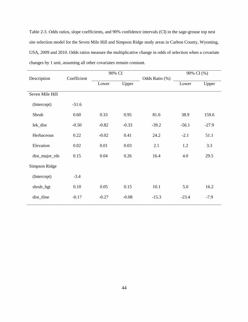
44
Table 2-3. Odds ratios, slope coefficients, and 90% confidence intervals (CI) in the sage-grouse top nest
site selection model for the Seven Mile Hill and Simpson Ridge study areas in Carbon County, Wyoming,
USA, 2009 and 2010. Odds ratios measure the multiplicative change in odds of selection when a covariate
changes by 1 unit, assuming all other covariates remain constant.
Description Coefficient 90% CI
Odds Ratio (%) 90% CI (%)
Lower Upper Lower Upper
Seven Mile Hill
(Intercept) -51.6
Shrub 0.60 0.33 0.95 81.6 38.9 159.6
lek_dist -0.50 -0.82 -0.33 -39.2 -56.1 -27.9
Herbaceous 0.22 -0.02 0.41 24.2 -2.1 51.1
Elevation 0.02 0.01 0.03 2.1 1.2 3.3
dist_major_rds 0.15 0.04 0.26 16.4 4.0 29.5
Simpson Ridge
(Intercept) -3.4
shrub_hgt 0.10 0.05 0.15 10.1 5.0 16.2
dist_tline -0.17 -0.27 -0.08 -15.3 -23.4 -7.9

45
Table 2-4. Model fit statistics for greater sage-grouse brood selection at the Seven Mile Hill and Simpson
Ridge study areas, Carbon County, Wyoming, USA, 2009 and 2010. Models are listed according to the
model best fitting the data and ranked by (ΔAICc), the difference between the model with the lowest
Akaike’s Information Criterion for small samples (AICc) and the AICc for the current model. The value
of the maximized log-likelihood function (log[L]), the number of estimated parameters (K), and Akaike’s
weights (wi) for each model are also presented.
Model log[L] K AICc ΔAICc wi
Seven Mile Hill
dist_tline, dist_tline2, bare ground460,
herbaceous1000, elevation1000, shrub1000 -309.9 7 635.1 0.00 0.91
dist_tline, dist_tline2, bare ground460,
herbaceous1000, elevation1000 -313.5 6 640.0 4.92 0.08
dist_tline, dist_tline2, bare ground460,
herbaceous1000 -316.9 5 644.5 9.45 0.01
dist_tline, dist_tline2, bare ground460 -323.4 4 655.3 20.22 0.00
dist_tline, dist_tline2 -343.4 3 693.1 57.99 0.00
Simpson Ridge
dist_tline, litter460, dist_major_rds, herbaceous1000,
bare ground300 -518.4 6 1049.8 0.00 0.81
dist_tline, litter460, dist_major_rds, herbaceous1000 -521.1 5 1052.9 3.15 0.17
dist_tline, litter460, dist_major_rds -524.2 4 1056.9 7.06 0.02
dist_tline, litter460 -527.4 3 1061.0 11.19 0.00
dist_tline -530.9 2 1065.9 16.08 0.00

46
Table 2-5. Odds ratios, slope coefficients, and 90% confidence intervals (CI) for covariates in the sage-
grouse top brood-rearing selection model for the Seven Mile Hill and Simpson Ridge study areas in
Carbon County, Wyoming, USA, 2009 and 2010. Odds ratios measure the multiplicative change in odds
of selection when a covariate changes by 1 unit, assuming all other covariates remain constant. Odds
ratios were not calculated for covariates involved with a quadratic effect because they were dependent on
values of other covariates.
Description Coefficient 90% CI
Odds Ratio (%) 90% CI (%)
Lower Upper Lower Upper
Seven Mile Hill
(Intercept) 19.3
dist_tline 1.12 NA NA NA NA NA
dist_tline2 -0.12 -0.25 -0.03 NA NA NA
Bare ground -0.14 -0.19 -0.09 -13.1 -17.5 -8.6
Herbaceous 0.68 0.25 1.28 96.5 27.8 260
Elevation -0.01 -0.02 0.00 -1.1 -2.28 -0.14
Shrub 0.42 0.01 0.95 52.7 1.1 158
Simpson Ridge
(Intercept) -1.0
dist_tline -0.12 -0.39 0.07 -11.0 -32.1 7.4
Litter 0.11 0.02 0.19 11.4 2.0 20.7
dist_major_rd 0.09 -0.05 0.28 9.2 -4.4 33.0
Herbaceous -0.09 -0.28 0.01 -9.0 -24.6 1.1
Bare ground -0.03 -0.06 -0.01 -3.3 -5.6 -1.1

47
Table 2-6. Model fit statistics for greater sage-grouse summer selection at the Seven Mile Hill and
Simpson Ridge study areas, Carbon County, Wyoming, USA, 2009 and 2010. Models are listed according
to the model best fitting the data and ranked by (ΔAICc), the difference between the model with the
lowest Akaike’s Information Criterion for small samples (AICc) and the AICc for the current model. The
value of the maximized log-likelihood function (log[L]), the number of estimated parameters (K), and
Akaike’s weights (wi) for each model are also presented.
Model log[L] K AICc ΔAICc wi
Seven Mile Hill
lek_dist, bare ground300, dist_major_rds, dist_turbine,
elevation1000 -1880.4 7 3774.1 0.00 1.00
lek_dist, bare ground300, dist_major_rds, dist_turbine -1915.1 6 3841.0 66.9 0.00
lek_dist, bare ground300, dist_major_rds, -1959.0 5 3926.7 152.6 0.00
lek_dist, bare ground300 -1983.4 3 3973.4 199.3 0.00
lek_dist -2045.0 2 4094.3 320.3 0.00
Simpson Ridge
lek_dist, bare ground1000, dist_major_rds,
dist_major_rds2, herbaceous1000,
Wyoming_sagebrush1000
-2625.4 7 5266.1 0.00 1.00
lek_dist, bare ground1000, dist_major_rds,
dist_major_rds2, herbaceous1000 -2648.2 6 5309.3 43.2 0.00
lek_dist, bare ground1000, dist_major_rds,
dist_major_rds2 -2688.7 5 5388.6 122.6 0.00
lek_dist, bare ground1000 -2780.3 3 5567.2 301.1 0.00
lek_dist -2963.4 2 5931.1 665.0 0.00

48
Table 2-7. Odds ratios, slope coefficients, and 90% confidence intervals (CI) for covariates in the sage-
grouse top summer selection model for the Seven Mile Hill and Simpson Ridge study areas in Carbon
County, Wyoming, USA, 2009 and 2010. Odds ratios measure the multiplicative change in odds of
selection when a covariate changes by 1 unit, assuming all other covariates remain constant. Odds ratios
were not calculated for covariates involved with a quadratic effect because they were dependent on values
of other covariates.
Description Coefficient 90% CI
Odds Ratio (%) 90% CI (%)
Lower Upper Lower Upper
Seven Mile Hill
(Intercept) -11.9
lek_dist -0.31 -0.49 -0.16 -26.5 -38.7 -15.0
bare ground -0.08 -0.10 -0.06 -7.3 -9.4 -5.4
dist_major_rds 0.16 0.07 0.26 17.1 7.3 29.0
dist_turbine -0.25 -0.41 -0.11 -22.4 -33.3 -10.7
elevation 0.01 0.00 0.01 0.76 0.27 1.3
Simpson Ridge
(Intercept) 5.63
lek_dist -0.25 -0.43 -0.11 -22.5 -35.3 -10.4
bare ground -0.14 -0.19 -0.08 -12.9 -17.6 -8.0
dist_major_rds 0.40 NA NA NA NA NA
dist_ major_rds2 -0.02 -0.05 0.00 NA NA NA
herbaceous -0.14 -0.26 -0.04 -13.4 -23.1 -4.0
wygenis 0.29 0.07 0.58 34.2 7.3 78.4

49
Figure 2-1. Odds ratios or relative probability of sage-grouse nest site selection and 90% confidence
intervals (dashed lines) within the Seven Mile Hill study area as a function of top model covariates,
Carbon County, Wyoming, USA, 2009 and 2010. All other covariates in the best approximating model
were held constant at their mean value. Overlapping confidence limits indicate a non-significant estimate.

50
Figure 2-2. Odds ratios or relative probability of sage-grouse nest site occurrence and 90% confidence
intervals (dashed lines) within the Simpson Ridge study area as a function of top model covariates,
Carbon County, Wyoming, USA, 2009 and 2010. All other covariates in the best approximating model
were held constant at their mean value.
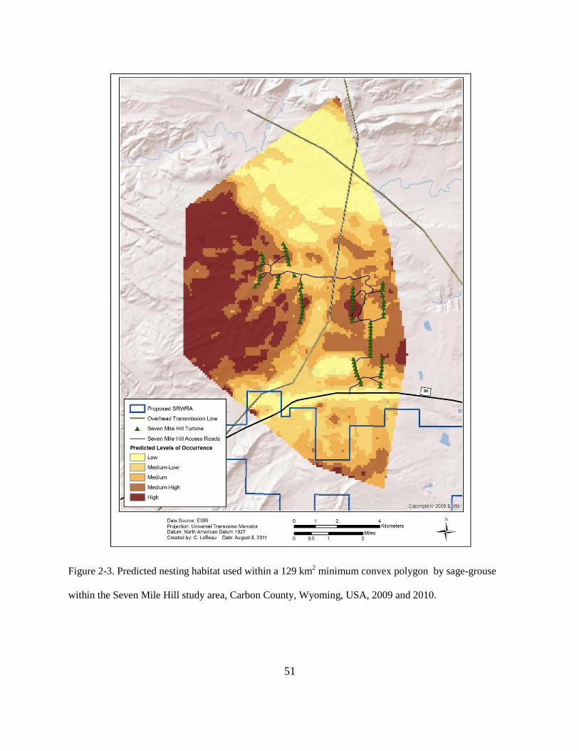
51
Figure 2-3. Predicted nesting habitat used within a 129 km2 minimum convex polygon by sage-grouse
within the Seven Mile Hill study area, Carbon County, Wyoming, USA, 2009 and 2010.

52
Figure 2-4. Predicted nesting habitat used within a 217 km2 minimum convex polygon by sage-grouse
within the Simpson Ridge Study area, Carbon County, Wyoming, USA, 2009 and 2010.

53
Figure 2-5. Odds ratios or relative probability of sage-grouse brood-rearing selection and 90% confidence
intervals (dashed lines) within the Seven Mile Hill study area as a function of top model covariates,
Carbon County, Wyoming, USA, 2009 and 2010. Confidence intervals were not calculated for distance to
transmission line because confidence intervals for quadratic effects depend on values of other covariates.

54
Figure 2-6. Odds ratios or relative probability of sage-grouse brood-rearing occurrence and 90%
confidence intervals (dashed lines) within the Simpson Ridge study area as a function of top model
covariates, Carbon County, Wyoming, USA, 2009 and 2010. All other covariates in the best
approximating model were held constant at their mean value. Overlapping confidence limits indicate a
non-significant estimate.

55
Figure 2-7. Predicted brood-rearing habitat used within a 126 km2 minimum convex polygon by sage-
grouse within the Seven Mile Hill study area, Carbon County, Wyoming, USA, 2009 and 2010.
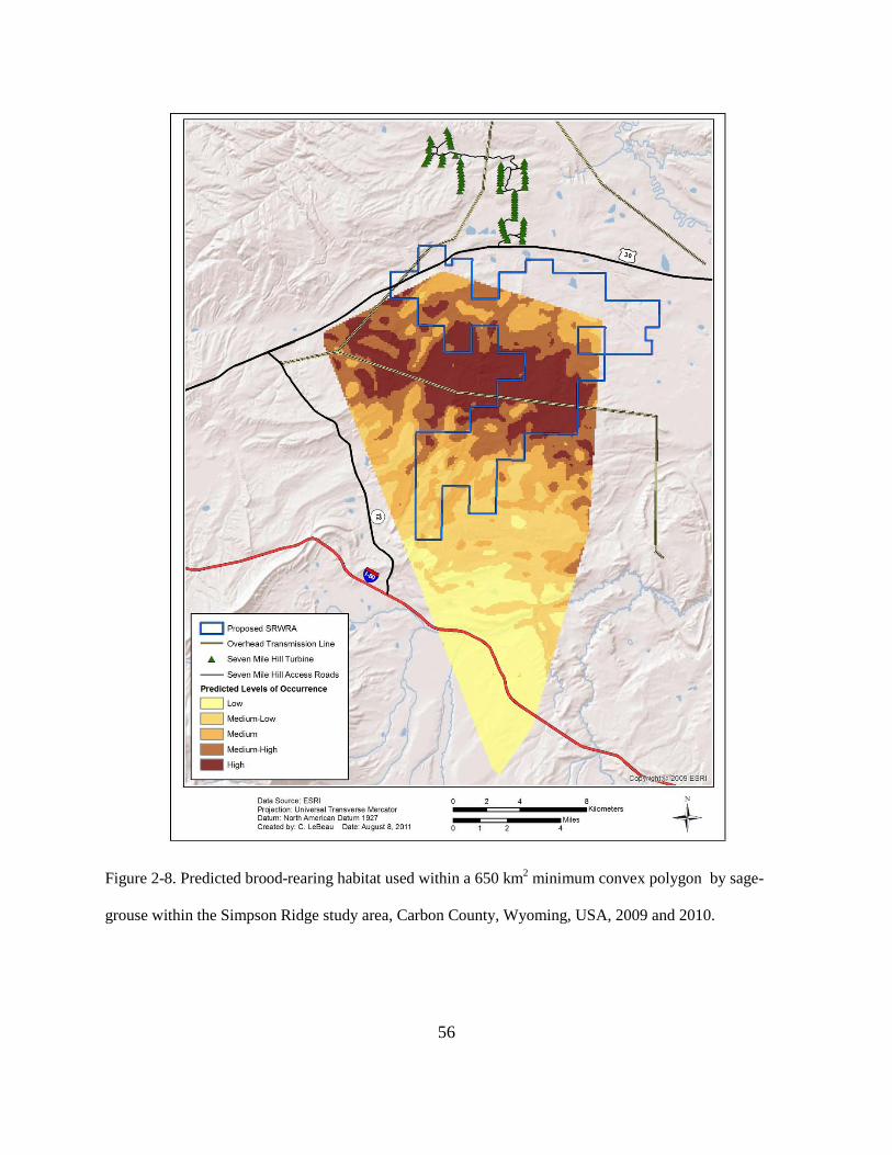
56
Figure 2-8. Predicted brood-rearing habitat used within a 650 km2 minimum convex polygon by sage-
grouse within the Simpson Ridge study area, Carbon County, Wyoming, USA, 2009 and 2010.

57
Figure 2-9. Odds ratios or relative probability of female sage-grouse summer occurrence and 90%
confidence intervals (dashed lines) within the Seven Mile Hill study area as a function of top model
covariates, Carbon County, Wyoming, USA, 2009 and 2010. All other covariates in the best
approximating model were held constant at their mean value.

58
Figure 2-10. Odds ratios or relative probability of female sage-grouse summer occurrence and 90%
confidence intervals (dashed lines) within the Simpson Ridge study area as a function of top model
covariates, Carbon County, Wyoming, USA, 2009 and 2010. All other covariates in the best
approximating model were held constant at their mean value. Confidence intervals were not calculated for
distance to major road because confidence intervals for quadratic effects depend on values of other
covariates.

59
Figure 2-11. Predicted summer habitat used within a 243 km2 minimum convex polygon by sage-grouse
within the Seven Mile Hill study area, Carbon County, Wyoming, USA, 2009 and 2010.

60
Figure 2-12. Predicted summer habitat used within a 751 km2 minimum convex polygon by sage-grouse
within the Simpson Ridge study area, Carbon County, Wyoming, USA, 2009 and 2010.

61
CHAPTER 3
Greater Sage-grouse Fitness Parameters Associated
with Wind Energy Development
In the format for manuscript submittal to the Journal of Wildlife Management
ABSTRACT
Greater sage-grouse (Centrocercus urophasianus) are experiencing population declines in much
their current range. Population declines are directly related to changes in greater sage-grouse
fitness parameters including nest success, brood success, and female survival. The overall fitness
of an individual ultimately determines if the individual is contributing to the viability of a
population. Reduced fitness leads to population declines because of the lack of the individual’s
contribution to the population. Reduced fitness in greater sage-grouse populations have been
attributed to a decrease in habitat suitability caused by invasive plant species, increased
predation, and energy extraction activities. More recently, the increased demand for clean
renewable energy has raised concerns about the impacts to greater sage-grouse fitness parameters
in habitats occupied by wind turbines. However, little is known about these potential impacts and
mine is the first study to estimate short-term impacts from wind energy development on greater
sage-grouse fitness parameters. I hypothesized greater sage-grouse fitness parameters decreased
with increasing proximity to wind energy infrastructure particularly wind turbines. I identified 88
nests from 2009 to 2010 within the Simpson Ridge and Seven Mile Hill study areas. In addition,
I monitored 31 females during the brood-rearing period to assess brood survival. Lastly, I
identified 45 mortalities of adult females within both study areas. I utilized Cox proportional
hazard regression to model nest survival and used the Andersen and Gill survival model to
estimate female survival and brood survival relative to wind turbines. I used forward model
62
selection and Akaike’s information criterion to determine optimal models for each fitness
parameter. I used Schoenfeld residuals to test for non-proportional hazards in the top model. The
results from the survival time analysis indicated the risk of a brood or nest failing increased
within habitats of close proximity to wind turbines. In addition, I detected no variation in female
survival relative to wind infrastructure. Future wind energy development should consider the
increased risk of brood and nest failure within habitats of close proximity to turbines. Identifying
nesting and brood-rearing habitats within close proximity to wind energy developments is critical
when estimating potential impacts to overall population fitness.
INTRODUCTION
The population demographics of greater sage-grouse (Centrocercus urophasianus; hereafter
sage-grouse) are unique among upland game bird species (Connelly et al. 2011). Sage-grouse
have relatively low reproductive rates (Connelly et al. 2000); low winter mortality (Wik 2002,
Zablan 2003), high annual survival (Holloran 1999), and many populations are migratory
(Connelly et al. 1988, 2000, Schroeder et al. 1999; Fedy et al. 2012). These demographics are
variable among subpopulations across the species’ range due to changes in environmental
gradients and anthropogenic influences (Connelly et al. 2011).
Nest success is an important vital rate of sage-grouse populations and can be used to
assess trends in population productivity. Nest success is defined as the probability of a nest
hatching one or more eggs successfully (Rotella et al. 2004). Poor nest success has often been
related to sage-grouse population declines (Crawford and Lutz 1985, Gregg et al. 1994,
Schroeder et al. 1999). The average nest success rate for sage-grouse in 29 studies using radio-
telemetry was 46% (range: 15–86%), and was widely dependent on region, habitat conditions,
and study design (Connelly et al. 2011). Nest success also differs from unaltered habitats (61%

63
of studies reported ≥50% and 22% of studies reported <40% overall nest success) to altered
habitats (17% of studies reported ≥50% and 42% of studies reported <40% overall nest success;
Connelly et al. 2011).
Peak egg-laying and incubation occurs from March through mid-June, with renesting
lasting into early July (Gregg 2006, Schroeder et al. 1999). Mean sage-grouse clutch size ranges
from 6.3 to 9.1 eggs (Schroeder et al. 1999). Female sage-grouse exhibit high fidelity to nesting
areas (Holloran and Anderson 2005, Fischer et al. 1993). They are known to nest on average 2.1
km from undisturbed leks of capture and 4.1 km from disturbed leks of capture in southwestern
Wyoming (Lyon and Anderson 2003). In Wyoming, nests that are not located in close proximity
to other nests and situated closest to leks tend to be more successful (Holloran and Anderson
2005). Nest propensity is variable across the species range averaging 78% (Connelly et al. 2011).
Furthermore, adult females tend to have higher nest initiation rates than yearlings (Connelly et al.
2004) and female sage-grouse may renest (mean: 30% in the western portion of the species
range) following their failed first nesting attempt (Connelly et al. 2011).
In addition to nesting success, early and late brood success is a key parameter in
assessing sage-grouse population demographics because juvenile survival impacts overall
population productivity (Crawford et al. 2004, Connelly et al. 2011). Beck et al. (2006) provided
estimates that indicate juvenile survival equals adult survival after 10 weeks of age, suggesting
that nesting and early brood-rearing success are critical drivers of population change. I defined
early brood success as the proportion of broods that survived 14 days post hatch (Thompson et
al. 2006) and late brood success as the proportion of broods that survived 35 days post hatch
(Walker 2008).
64
Sage-grouse chick survival during the early brood period (18 days post hatch) has been
estimated to be 44% in southeastern Oregon and northern Nevada (Rebholz 2007), and 39%
through day 28 in south-central Oregon and northern Nevada (Gregg 2006). Chick survival
during the late brood period (35 days post hatch) has been estimated to be 33–50% in
northeastern Wyoming and southeastern Montana (Walker 2008) and 76.2% (40 days post hatch)
in southeastern Wyoming (Kirol 2012). Early brood activity occurs in the vicinity of nesting
locations (mean distance from nest in southwestern Wyoming was 1.1 km; Lyon 2000), with the
habitat characterized as having a healthy sagebrush (Artemisia spp.) overstory and herbaceous
understory containing insects critical to chick survival (Johnson and Boyce 1990). When
landscapes become desiccated around midsummer, brooding hens often migrate 5-82 km from
early brood-rearing habitat (Klebenow and Gray 1968, Wallestad 1971, Connelly et al. 1988,
Fisher et al. 1997) to more forb rich habitat, usually higher in elevation where pockets of
moisture still remain (Klebenow 1969). These brooding habitats are widely variable and in many
cases are dependent on yearly weather conditions (Patterson 1952, Dalke et al. 1963, Connelly et
al. 1988, Gregg et al. 1993, Wallestad 1971).
Sage-grouse declines are at least partially explained by lower annual survival of female
sage-grouse and in the case of oil and gas development, the impacts to survival result in
population-level declines (Holloran 2005). Sage-grouse are characterized as having high annual
survival compared to other upland game birds. Annual survival rates of adult female sage-grouse
in Wyoming were estimated to be 48–78% (Holloran 1999, 2005). Seasonal survival is variable
for both male and female sage-grouse, but is highest during the winter (88–100%; Wik 2002,
Beck et al. 2006) and lowest during the spring (57%, March-June; Connelly et al. 2000),
summer, and fall (Connelly et al. 2000, Wik 2002).

65
The purpose of my study was to investigate the affect of wind energy infrastructure on
sage-grouse fitness parameters. Specifically, I investigated sage-grouse nest, brood, and female
survival in relation to wind energy infrastructure including turbines, roads, and transmission
lines. I hypothesized that sage-grouse nest, brood, and female survival decreased as proximity to
infrastructure, specifically turbines, increased. This information is critical to provide for use in
planning future wind energy development sites that occur within occupied sage-grouse habitats.
STUDY AREA
My study area was consistent with Chapters 1 and 2 in this thesis. Observed nests, brood
locations, and mortality locations were combined between years and study areas for my survival
analysis (see Fig. 1-1).
METHODS
Field Methods
I captured 116 female sage-grouse by spotlighting and use of hoop nets (Giesen et al. 1982,
Wakkinen et al. 1992) on roosts surrounding leks during the 2009 and 2010 breeding seasons.
Initial capture efforts were centered within SR during the first study year (2009) where 50 sage-
grouse females were targeted and 25 were targeted within SMH. During the second study season
(2010) the target sample size increased to 40 at SMH and 45 at SR. I attempted to capture grouse
at all accessible active lek sites within 16 km of the SMH wind turbines proportionately to the
number of males attending those leks. I aged, weighed (0.1-g precision), acquired blood samples
(year 2009), and fitted each captured grouse with a 22-g necklace-mounted radio transmitter with
a battery life of 666 days (Advanced Telemetry Systems, Isanti, MN). I then released each radio-
marked female grouse at the point of capture and marked the location using a hand held global
positioning system (GPS) unit.

66
I relocated each radio-marked female at least twice each week during the prelaying and
nesting period (Apr through Jun); once every week for brooding females during the brood-
rearing period (hatch through 15 Aug); and, at least once per week during the summer (Jun
through 1 Nov) periods for all barren females (i.e., females that were unsuccessful in producing
or raising young or were not currently nesting or raising young). Marked sage-grouse were
monitored primarily from the ground using hand-held receivers. I determined sage-grouse
locations by triangulation or homing until visibly observed and classified radio-locations as
breeding, nesting, brood-rearing, or summer. Triangulation locations were estimated by taking
two vectors in the direction of the signal. In addition, I estimated the triangulation error by
placing 6 test collars for each technician throughout both project areas and estimated the mean
telemetry error between the actual and estimated locations. The mean error telemetry rate was
incorporated into the habitat selection modeling effort. I employed aerial telemetry to locate
missing birds throughout the study period.
I determined nesting success for each radio-marked female sage-grouse from long range
triangulation at least every third day throughout the nesting season, late April through 15 June. I
assumed females were nesting when movements became localized. Nests were located using a
progressively smaller concentric circle approached by walking circles around the radio signal
using the signal strength as an indication of proximity (Holloran and Anderson 2005). Once I
visually confirmed the female in an incubating position, the location of the observer was
recorded with a GPS and a photograph was taken of the habitat surrounding the incubating hen.
All future monitoring of the nest was made from remote locations (>60 m) using long distance
triangulation to minimize potential disturbance. Once a nest location was established, I
conducted incubation monitoring on an alternate-day schedule to determine nesting fate. For

67
each nest and re-nest, I collected data on timing of incubation and nest success. All nest locations
were mapped using a hand-held GPS. A nest that successfully hatched (i.e., eggs with detached
membranes) ≥1 egg was considered a successful nesting attempt. Nests that failed to successfully
hatch ≥1 egg were considered failed nesting attempts whose fates included predation (avian,
mammal, and unknown) and abandoned. Females that were unsuccessful in their first nesting
attempt were monitored three times per week to determine possible re-nesting attempts. Females
that were unsuccessful in their first or second nesting attempt were monitored twice each week
through 1 November in 2009 and 2010.
I located radio-marked females that successfully hatched ≥1 egg each week through 15
August 2009 and 2010 to evaluate brood-rearing habitat selection. I categorized the brood-
rearing period as early (hatch through 14 days post-hatch; Thompson et al. 2006) or late (35 days
post-hatch; Walker 2008). Females were considered successful through the early brood-rearing
period if ≥1 chick survived to two weeks post-hatch; chick presence during this period was
established either through visual confirmation of a live chick or the brooding female’s response
to the researcher (e.g., chick protective behavior exhibited). I determined fledging success (late
brood success) for those females who were successful in early brood-rearing by assessing
whether a female was brooding chicks through nighttime spotlight surveys conducted on days 35
and 36 post-hatch (Walker 2008). Similar to sage-grouse with unsuccessful nests, sage-grouse
that were unsuccessful during either the early or late brood-rearing period were monitored twice
each week through 31 August.
GIS Covariates
I developed a suite of covariates to estimate the variability in nest, brood, and female survival
within both study areas. Anthropogenic features included major roads, transmission lines, and

68
turbines. Major roads included paved highways: U.S. Highway 30/287 traversed east-west
separating SR from SMH; Wyoming State Highway 72 traversed north-south through the SR
study area; and Interstate 80 traversed east-west south of the SR study area (see Fig. 1-1). The
SMH study area included wind turbines and access roads whereas the SR did not. Major roads
and overhead transmission lines were digitized using aerial satellite imagery and ArcMap 10
(ESRI 2011). Turbine locations were obtained from PacifCorp, the operators of the SMH Wind
Energy Facility.
Environmental covariates I considered included vegetation and topographic features
within both study areas. Vegetation layers used in the analysis were remote sensed sagebrush
products developed by Homer et al. (2012). This dataset used a combination of methods to
integrate 2.4 m QuickBird, 30 m Landsat TM, and 56 m AWiFS (Advanced Wide Field Sensor)
imagery into the characterization of four primary continuous field components (percent bare
ground, percent herbaceous cover, percent litter, and percent shrub cover) and four secondary
components (three subdivisions of shrub cover —percent sagebrush (Artemisia spp.), percent big
sagebrush (A. tridentata spp.), and percent Wyoming big sagebrush (A. t. wyomingensis)—and
shrub height, using regression classification (Homer et al. 2009, 2012; Table 3-1). Landscape
features included elevation, slope, and terrain ruggedness all of which were calculated from a 10
m National Elevation Dataset (USGS, EROS Data Center, Sioux Falls, SD). Terrain ruggedness
captured the variability in slope and aspect into a single measure ranging from 0 (no terrain
variation) to 1 (complete terrain variation; Sappington et al. 2005; Table 3-1).
Survival Parameters
The most common method used to estimate nest survivorship is the Mayfield method (Mayfield
1961, 1975, Burhans et al. 2002, Liebeziet and George 2002, Nur et al. 2004); however, this
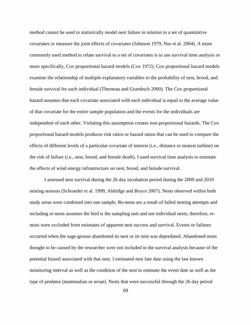
69
method cannot be used to statistically model nest failure in relation to a set of quantitative
covariates or measure the joint effects of covariates (Johnson 1979, Nur et al. 2004). A more
commonly used method to relate survival to a set of covariates is to use survival time analysis or
more specifically, Cox proportional hazard models (Cox 1972). Cox proportional hazard models
examine the relationship of multiple explanatory variables to the probability of nest, brood, and
female survival for each individual (Therneau and Grambsch 2000). The Cox proportional
hazard assumes that each covariate associated with each individual is equal to the average value
of that covariate for the entire sample population and the events for the individuals are
independent of each other. Violating this assumption creates non-proportional hazards. The Cox
proportional hazard models produces risk ratios or hazard ratios that can be used to compare the
effects of different levels of a particular covariate of interest (i.e., distance to nearest turbine) on
the risk of failure (i.e., nest, brood, and female death). I used survival time analysis to estimate
the effects of wind energy infrastructure on nest, brood, and female survival.
I assessed nest survival during the 26 day incubation period during the 2009 and 2010
nesting seasons (Schroeder et al. 1999, Aldridge and Boyce 2007). Nests observed within both
study areas were combined into one sample. Re-nests are a result of failed nesting attempts and
including re-nests assumes the bird is the sampling unit and not individual nests; therefore, re-
nests were excluded from estimates of apparent nest success and survival. Events or failures
occurred when the sage-grouse abandoned its nest or its nest was depredated. Abandoned nests
thought to be caused by the researcher were not included in the survival analysis because of the
potential biased associated with that nest. I estimated nest fate date using the last known
monitoring interval as well as the condition of the nest to estimate the event date as well as the
type of predator (mammalian or avian). Nests that were successful through the 26 day period

70
were censored (Nur et al. 2004). I used Cox proportional hazards to estimate the effects of wind
energy infrastructure on nest survival (Nur et al. 2004, Aldridge and Boyce 2007, Liebezeit et al.
2009).
In addition to nest survival, I estimated brood survival within both study areas. Female
sage-grouse successfully hatching at least 1 egg during the nesting season were monitored at
least once each week from time of hatch to 35 days post hatch; however, to determine brood
survival I assessed the presence of chicks with hens at least 2 times during the first 14 days of the
brood-rearing period and one final time at the end of the 35 day brood-rearing period. All early
and late brood-rearing locations from both study areas and years were combined and included in
the survival modeling. Events or failures occurred when no chicks were observed or the female
did not act as if she had chicks during either one of the checks. I estimated the fate date using the
last monitoring interval where chick survival was assessed. Broods that were successful through
the 35 day period were censored (Nur et al. 2004). I used weekly monitoring intervals during this
period to assess brood survival. The first monitoring interval began directly after a successful
hatched nest and ended 37 days post hatch (Walker 2008). Intervals that recorded multiple
observations were grouped and their corresponding covariates were averaged.
Lastly, I modeled female sage-grouse survival from time of capture to 31 October during
both years. Female sage-grouse were monitored at least once each week during this period, thus I
assessed weekly survival for all monitored sage-grouse. Events or mortalities occurred when I
confirmed mortality via telemetry. I estimated fate date by the condition of the carcass and last
known monitoring interval. I grouped intervals that recorded multiple observations and averaged
their corresponding covariates.
Model Development

71
I estimated nest survival using Cox proportional hazards (Cox 1972); however, I used the
Anderson-Gill model (A-G; Anderson and Gill 1982), a formulation of the Cox proportional
hazards model, to model brood and female survival. The A-G model accommodates left and right
censored observations, continuous and categorical covariates that may vary during monitoring,
and discontinuous intervals of risk, which are the product of missed observations or
measurements (Therneau and Grambsch 2000, Johnson et al. 2004). The A-G model uses a
counting process style of data input where each subject is represented as a series of observations
with time intervals (i.e., sage-grouse brood location during a single monitoring interval). This
allowed me to incorporate varying degrees of habitat units used throughout the interval of risk.
I used a forward model selection procedure to identify the effects of wind energy
infrastructure on nest, brood, and female survival. Because many of my covariates were
correlated (r ≥ |6|), I allowed for each covariate to compete with each other in a forward selection
procedure. However, I did not allow two correlated variables to be included in any one model. I
included an indicator variable for which study area the sage-grouse was captured from (SMH=1,
SR= 0) and the age of the sage-grouse (adult = 1, juvenile = 0) to determine if age or study area
was influencing survival. In addition, the average values representing each environmental feature
were extracted at 3 different radii scales, the mean telemetry error rate (0.30 km), the median
distance between consecutive year’s nests from 2009 to 2010 within both study areas (0.46 km),
and the median distance traveled between monitoring intervals during the brood-rearing and
summer period (1.0 km). The median movement distance was 1.0 km during brood-rearing and
1.6 km during the summer season; however, I used 1.0 km based on findings from previously
published sage-grouse habitat selection studies (Aldridge and Boyce 2007, Carpenter et al.
2010). Kirol (2012) found the SD of shrub height to be an important predictor of nest survival in

72
south-central Wyoming; subsequently I included the SD of shrub height, shrub, and sagebrush in
my modeling procedure.
I identified the best approximating model by comparing the adjusted Akaike’s
Information Criterion (AICc; Burnham and Anderson 2002) values between models to identify
the model with the lowest AICc value. The top model was identified to be at least 4 ∆AICc
values from the next approximating model (Arnold 2010). I model averaged across the 90%
confidence set of competing models to estimate the final parameters of the top model to produce
more robust estimates and to address model uncertainty in competing models (Burnham and
Anderson 2002, Arnold 2010). I calculated hazard ratios and 90% hazard ratio confidence
intervals to interpret the magnitude of habitat and anthropogenic variables on an individual nest,
brood, or female sage-grouse’s daily or weekly hazard during the nesting, brooding-rearing, and
female survival periods. Estimates that included 0.0 within their 90% confidence interval were
considered insignificant (alpha level = 0.10). I used survival curves to illustrate the varying
degree of risk as a function of the top model covariates (Johnson et al. 2004, Therneau and
Grambsch 2000). I applied the coefficients generated from the top survival model to a logistic
regression equation to predict the odds of survival from 2009 through 2010 at both study areas
(Johnson et al. 2004).
Lastly, I used Schoenfeld residuals (Schoenfeld 1982) to assess model fit (Therneau et al.
1990). Scoring Schoenfeld residuals can be a powerful technique to test for non-proportional
hazards for continuous variables (Grambsch and Therneau 1994). Schoenfeld residuals for each
covariate in the top model are defined for every individual that has a failure event (Kleinbaum
and Klein 2005). For the proportional hazard assumption to hold true, the Schoenfeld residuals
for a particular covariate would not be related to survival time. I ranked the Schoenfeld residuals

73
for each covariate in the order of event failures (i.e., the individual with the first event gets a
value of 1, and so on; Kleinbaum and Klein 2005). I plotted the ranked Schoenfeld residuals for
each covariate and for the top model as a whole against time to inspect the distribution of the
residuals. I fitted a line to the residuals to test for a nonzero slope. A nonzero slope indicated
heterogeneity in the residuals thus, rejecting the null hypothesis that the correlation between the
Schoenfeld residuals and survival time was zero. Rejection of the null hypothesis indicates that
the proportional hazard assumption was violated.
RESULTS
Nest Survival
I located 95 nests in 2009 and 2010 (SR, n = 53; SMH, n = 42). During both study years, nesting
propensity, the number of females observed initiating a nesting attempt, ranged from 59.4%
(90% CI: 43.3–74.0%) to 77.3% (90% CI: 58.0–90.6%) within both study areas. SR had more
nests during both study years compared to SMH; however, SMH had 6 re-nest attempts
compared to 1 re-nest attempt at SR.
Two of the 6 observed re-nests within SMH were successful and the 1 re-nest observed
within SR was unsuccessful. Nest success was similar in 2009 and 2010 within both study areas,
ranging from 41.9% to 42.9% at SR and from 31.6% to 35.3% at SMH. Overall, nest success at
SR (42.3%; 90% CI: 30.7–54.6%, n = 52) was higher than at SMH (33.3%; 90% CI: 20.5–
48.3%, n = 36); however, the difference in the means was not statistically different. Nest hatch
dates ranged from 26 May to 28 June (mean = 1 Jun) for all assumed first nesting attempts and
from 29 June to 2 July (mean = 30 Jun) for all second nesting attempts.
During the 2009 and 2010 monitoring seasons, 16 first nesting attempt nests were
initiated within 1.6 km of wind turbines at SMH; the five nests closest to turbines were located

74
137 m, 231 m, 248 m, 257 m, and 333 m from the nearest turbine. Four of the 16 nests (25.0%)
within 1.6 km of turbines were successful, but none of the 5 nests closest to turbines were
successful.
The proximity of the observed nests to each infrastructure feature varied throughout the
study area. The mean distance to major roads and SMH turbines was greater for all successful
nests (6.5 km [90% CI: 5.5–7.4 km] and 8.3 km [90% CI: 6.3–10.2 km], respectively) compared
to failed nests (5.6 km [90% CI: 5.1–6.2 km] and 6.6 km [90% CI: 5.4–7.9 km], respectively);
however, these differences were not statistically different.
Model Fit.—Eighty-eight sage-grouse nests were used in Cox proportional hazard
modeling. The median duration of failed nesting attempts was estimated at 12 days. Results of
the univariate model estimating differences in survival among study areas indicated that study
area did not influence nest survival (hazard ratio = 1.2, 90% CI: 0.76–1.9). Three models
including environmental and anthropogenic covariates were within 2.5 ΔAICc of each other. I
model averaged the three competing models to estimate the final parameters for the top model
(Burnham and Anderson 2002; Table 3-2). The top model relating environmental and
anthropogenic features to sage-grouse nest survival included the standard deviation of shrub
height (cm) within 0.30 km of a nest and distances (km) to nearest turbine and nearest overhead
transmission line (Table 3-2).
The risk or the odds of a nest failing increased by 11.1% [(exp(𝛽0)-1)*100] with every
1.0 km increase in the distance to nearest overhead transmission line (90% CI: 10.1–12.1%;
Table 3-3; Fig. 3-1). The risk of a nest failing decreased by 14.4% for every 1 cm increase in the
SD of shrub height (cm) within 0.30 km of a nest (90% CI: 13.1–15.8%; Table 3-3; Fig. 3-1).
Similarly, the risk of a nest failing decreased by 6.2% as distance from turbine increased by 1 km
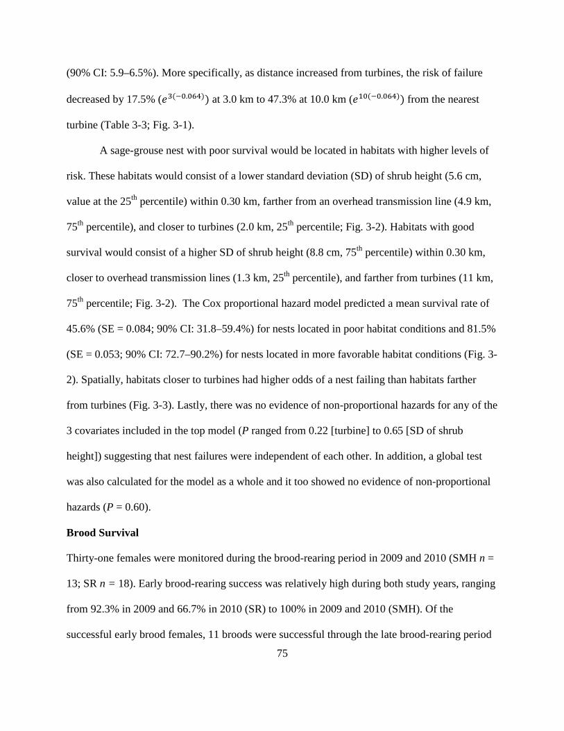
75
(90% CI: 5.9–6.5%). More specifically, as distance increased from turbines, the risk of failure
decreased by 17.5% (𝑒3(−0.064)) at 3.0 km to 47.3% at 10.0 km (𝑒10(−0.064)) from the nearest
turbine (Table 3-3; Fig. 3-1).
A sage-grouse nest with poor survival would be located in habitats with higher levels of
risk. These habitats would consist of a lower standard deviation (SD) of shrub height (5.6 cm,
value at the 25th percentile) within 0.30 km, farther from an overhead transmission line (4.9 km,
75th percentile), and closer to turbines (2.0 km, 25th percentile; Fig. 3-2). Habitats with good
survival would consist of a higher SD of shrub height (8.8 cm, 75th percentile) within 0.30 km,
closer to overhead transmission lines (1.3 km, 25th percentile), and farther from turbines (11 km,
75th percentile; Fig. 3-2). The Cox proportional hazard model predicted a mean survival rate of
45.6% (SE = 0.084; 90% CI: 31.8–59.4%) for nests located in poor habitat conditions and 81.5%
(SE = 0.053; 90% CI: 72.7–90.2%) for nests located in more favorable habitat conditions (Fig. 3-
2). Spatially, habitats closer to turbines had higher odds of a nest failing than habitats farther
from turbines (Fig. 3-3). Lastly, there was no evidence of non-proportional hazards for any of the
3 covariates included in the top model (P ranged from 0.22 [turbine] to 0.65 [SD of shrub
height]) suggesting that nest failures were independent of each other. In addition, a global test
was also calculated for the model as a whole and it too showed no evidence of non-proportional
hazards (P = 0.60).
Brood Survival
Thirty-one females were monitored during the brood-rearing period in 2009 and 2010 (SMH n =
13; SR n = 18). Early brood-rearing success was relatively high during both study years, ranging
from 92.3% in 2009 and 66.7% in 2010 (SR) to 100% in 2009 and 2010 (SMH). Of the
successful early brood females, 11 broods were successful through the late brood-rearing period
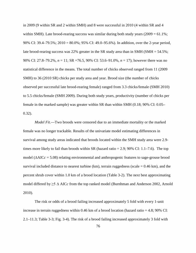
76
in 2009 (9 within SR and 2 within SMH) and 8 were successful in 2010 (4 within SR and 4
within SMH). Late brood-rearing success was similar during both study years (2009 = 61.1%;
90% CI: 39.4–79.5%; 2010 = 80.0%; 95% CI: 49.0–95.6%). In addition, over the 2-year period,
late brood-rearing success was 22% greater in the SR study area than in SMH (SMH = 54.5%;
90% CI: 27.8–79.2%, n = 11; SR =76.5, 90% CI: 53.6–91.0%, n = 17); however there was no
statistical difference in the means. The total number of chicks observed ranged from 11 (2009
SMH) to 36 (2010 SR) chicks per study area and year. Brood size (the number of chicks
observed per successful late brood-rearing female) ranged from 3.3 chicks/female (SMH 2010)
to 5.5 chicks/female (SMH 2009). During both study years, productivity (number of chicks per
female in the marked sample) was greater within SR than within SMH (0.18; 90% CI: 0.05–
0.32).
Model Fit.—Two broods were censored due to an immediate mortality or the marked
female was no longer trackable. Results of the univariate model estimating differences in
survival among study areas indicated that broods located within the SMH study area were 2.9-
times more likely to fail than broods within SR (hazard ratio = 2.9; 90% CI: 1.1–7.6). The top
model (ΔAICc = 5.08) relating environmental and anthropogenic features to sage-grouse brood
survival included distance to nearest turbine (km), terrain ruggedness (scale = 0.46 km), and the
percent shrub cover within 1.0 km of a brood location (Table 3-2). The next best approximating
model differed by ≥5 Δ AICc from the top ranked model (Burnhman and Anderson 2002, Arnold
2010).
The risk or odds of a brood failing increased approximately 5 fold with every 1-unit
increase in terrain ruggedness within 0.46 km of a brood location (hazard ratio = 4.8; 90% CI:
2.1–11.3; Table 3-3; Fig. 3-4). The risk of a brood failing increased approximately 3 fold with

77
every 1.0% increase in percent shrub cover within 1.0 km of a brood location (hazard ratio = 3.0;
90% CI: 1.5–6.2; Table 3-4; Fig. 3-4). Lastly, the risk of a brood failing decreased by 38.1%
with every 1.0 km increase in distance from nearest turbine (hazard ratio = 0.619; 90% CI: 18.6–
52.9%; Table 3-3; Fig. 3-4). More specifically, while holding other covariates constant, the effect
of a 0.50 km increase in distance to nearest turbine decreased the risk of brood failure by 21.3%.
As distance increased from turbine, the relative risk of failure decreased from 76.2% at 3 km to
97.8% at 8 km from the nearest turbine (Fig. 3-4). Spatially, habitats closer to turbines had
higher odds of a brood failing than habitats farther from turbines (Fig. 3-5). Lastly, there was no
evidence of non-proportional hazards for any of the 3 covariates included in the top model (P
ranged from 0.29 [rugged460] to 0.80 [turbine]) suggesting that brood failures were independent
of each other. In addition, a global test calculated for the model as a whole showed no evidence
of non-proportional hazards (P = 0.20).
Female Survival
During the study, 45 of 116 (38.8%) radio-marked birds died. I recorded 31 mortalities in SR (15
in 2009 and 16 in 2010) and 14 within SMH (5 in 2009 and 9 in 2010). Although cause of death
could not be determined for all mortalities, 13 were determined to be killed by avian predators
and 16 were determined to be killed by mammalian predators. In 2009, 3 dead radio-collared
females that did not exhibit any signs of trauma were submitted to the Wyoming State Veterinary
Lab in Laramie, Wyoming to be examined for the presence of West Nile virus. Two of the 3
female sage-grouse tested positive for West Nile virus and all were located within the SR study
area. The median distance of mortality locations to each infrastructure feature varied from 4.0
km (overhead transmission line), to 6.7 km (major roads), to 8.7 km (turbine). The mean female

78
survival rate at SMH was 28.0% (90% CI: 18.1–40.4%) compared to 47.0% (90% CI: 36.5–
57.7%) at SR.
Model Fit.–A total of 1,417 locations, 23 monitoring intervals, and 45 mortalities were
used to model female sage-grouse survival. Eight mortality events were censored because they
occurred within 2 weeks of capture. The univariate model estimating differences in female
survival among study areas indicated that study area (SMH vs. SR) did not influence female
survival (hazard ratio = 0.84; 90% CI: -0.73–0.36). Adult females were 1.3-times more likely to
die than juvenile females (hazard ratio = 1.3; 90% CI: 0.75–2.2). I experienced some model
uncertainty and modeled averaged the 95% confidence set of top models (Table 3-2).The top
model (ΔAICc = 0.55) relating environmental and anthropogenic features to female survival
included distance (km) to nearest major road and overhead transmission line (Table 3-2).
However, this model (AICc = 378.9) was not more explanatory (within 4 AICc points) than the
null model (AICc = 379.3), suggesting none of the predictors I used were adequate to explain the
variation in survival within my study (Table 3-2). However, the risk of female mortality during
the survival period increased by 21.0% with every 1.0 km increase in distance from major roads
(90% CI: 16.4–24.9%; Table 3-3, Fig. 3-6). Similarly, the risk of mortality increased by 9.4%
with every 1.0 km increase in distance from transmission line (90% CI: 8.5–10.2%; Table 3-3,
Fig. 3-6). Spatially, habitats closer to transmission lines had a higher odds of survival than
habitats farther from transmission lines (Fig. 3-7). There was no evidence of non-proportional
hazards for any of the 2 covariates included in the top model (P = 0.86 for major roads and P =
0.81 for overhead transmission line) suggesting that summer mortalities were independent of
each other. In addition, a global test was also calculated for the model as a whole and it too
showed no evidence of non-proportional hazards (P = 0.95).

79
DISCUSSION
I investigated the potential influence of wind energy development 2 yrs post development,
particularly wind turbine influences on sage-grouse nests, broods, and female survival because
these parameters have the greatest effect on sage-grouse population growth (Taylor et al. 2012).
More specifically, female survival and brood survival, in that order, have the greatest effect on
sage-grouse population growth rate (Taylor et al. 2012). I hypothesized that risk of failure
increased for nests and broods that were in close proximity to turbines. In addition, I
hypothesized that the risk of female mortality increased as proximity to turbines decreased. I
determined that the risk of sage-grouse nest and brood failure increased as proximity to turbines
increased using Cox proportional hazards and the Andersen-Gill formulation of Cox proportional
hazards. Overall female survival was not influenced by proximity to turbines or any other
landscape habitat feature used in the analysis; however, female survival was highest around
transmission lines throughout the study area.
The reason for the decreased nest and brood survival within habitats in close proximity to
turbines is unknown but may be attributed to increased predation (Coates and Delhanty 2010)
due to the presence of human development and edge effects (Batary and Baldi 2004). The lack of
concurrent predator monitoring makes it difficult to speculate why there is a decrease in survival
closer to turbines. The incorporation of different covariates (i.e., predator densities, noise, and
detailed weather data) may further explain the variation in survival among sage-grouse occurring
in habitats with close proximity to wind energy.
Nest success within SMH (33.3%) was similar to other sage-grouse studies that reported
nest success in other habitats influenced by other forms of energy development (<40%; Connelly
et al. 2011). Nest success at SR (42.3%) was slightly higher than at SMH (33.3%), but not as

80
high as the majority of studies in unaltered habitats (11 of 18 [61%] of studies reported ≥50%;
Connelly et al. 2011).
Survival time analysis or Cox proportional hazard modeling is becoming a widely used
and effective tool to predict nest survivorship in avian species (Liebezeit et al. 2009, Nur et al.
2004, Kirol 2012). Survival time analysis has been incorporated into sage-grouse studies as an
effective modeling procedure aimed at identifying risky habitats and specific covariates
influencing nest and brood survival (Aldridge and Boyce 2007, Moynahan et al. 2007, Herman-
Brunson et al. 2009, Kolada et al. 2009). Logistic regression (Holloran et al. 2005) and the
Mayfield method (Mayfield 1961, 1975) are also two other common methods for estimating nest
survivorship; however they have some limitations. Logistic regression is commonly used when
analyzing nest success in avian species (Holloran et al. 2005, Nur et al. 2004); however, it may
be inefficient and in some cases may introduce bias into the analyses because nests with
uncertain fates must be excluded from the analysis (Manolis et al. 2000). The Mayfield method
(Mayfield 1961, 1975) is the most common method at estimating nest survivorship in avian
studies; however, it is met with several restrictive and unrealistic assumptions including nest
failure is constant over time, homogeneity of failure probability, and independence of outcome
among nests (Dinsmore et al. 2002, Nur et al. 2004). Unlike logistic regression and the Mayfield
method, survival time analysis accounts for these assumptions.
The results of my nest survival time analysis indicated that nest survival within both
study areas was influenced by proximity to turbines and the variation in shrub height. The risk of
nest failure increased as proximity to turbines decreased and as the variation in shrub height
decreased. Similar sage-grouse nest survival studies indicated that the risk of nest failure was
positively influenced by greater shrub cover, higher grass height, grass cover, and greater
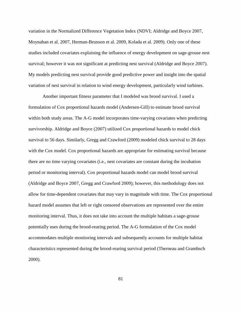
81
variation in the Normalized Difference Vegetation Index (NDVI; Aldridge and Boyce 2007,
Moynahan et al. 2007, Herman-Brunson et al. 2009, Kolada et al. 2009). Only one of these
studies included covariates explaining the influence of energy development on sage-grouse nest
survival; however it was not significant at predicting nest survival (Aldridge and Boyce 2007).
My models predicting nest survival provide good predictive power and insight into the spatial
variation of nest survival in relation to wind energy development, particularly wind turbines.
Another important fitness parameter that I modeled was brood survival. I used a
formulation of Cox proportional hazards model (Andersen-Gill) to estimate brood survival
within both study areas. The A-G model incorporates time-varying covariates when predicting
survivorship. Aldridge and Boyce (2007) utilized Cox proportional hazards to model chick
survival to 56 days. Similarly, Gregg and Crawford (2009) modeled chick survival to 28 days
with the Cox model. Cox proportional hazards are appropriate for estimating survival because
there are no time varying covariates (i.e., nest covariates are constant during the incubation
period or monitoring interval). Cox proportional hazards model can model brood survival
(Aldridge and Boyce 2007, Gregg and Crawford 2009); however, this methodology does not
allow for time-dependent covariates that may vary in magnitude with time. The Cox proportional
hazard model assumes that left or right censored observations are represented over the entire
monitoring interval. Thus, it does not take into account the multiple habitats a sage-grouse
potentially uses during the brood-rearing period. The A-G formulation of the Cox model
accommodates multiple monitoring intervals and subsequently accounts for multiple habitat
characteristics represented during the brood-rearing survival period (Therneau and Grambsch
2000).

82
The results of my brood survival analysis indicated that the risk of a brood failing
increased as proximity to turbines increased, as terrain ruggedness increased, and percent shrub
cover increased. Of the studies that utilized Cox survival model, brood survival was positively
correlated with grass cover (Gregg and Crawford 2009), risk of failure increased in habitats with
higher visible oil and gas well density within 1.0 km, and failure increased in habitats with
higher CTI (soil moisture index; Aldridge and Boyce 2007).
Lastly, estimating adult female survival is useful in understanding animal population
trends because it compares the cumulative effects of environmental conditions or anthropogenic
influences to the overall persistence of the population or the growth rate (λ). Sage-grouse
declines are at least partially explained by lower annual survival of female sage-grouse and in the
case of oil and gas development, the impacts to survival result in population-level declines
(Holloran 2005).
I used the A-G model to estimate female survival in summer in relation to wind energy
infrastructure. The top model did not differ from the null model suggesting the covariates I
measured within both study areas did not detect any variability in survival across the landscape.
However, the risk of mortality decreased in habitats with close proximity to transmission lines
and major roads. Similar to my study, Moynahan et al. (2006) found no support for inclusion of
landscape-level habitat variables in modeling monthly annual survival rates of sage-grouse in
Montana.
MANAGEMENT IMPLICATIONS
Mine is the first study to evaluate short term effects of wind energy infrastructure, specifically
turbines, on sage-grouse fitness parameters. The presence of turbines negatively impacted sage-
grouse nest and brood survival, whereas the presence of turbines did not appear to be affecting

83
female survival. Future wind energy project placement should consider the increased levels of
risk to sage-grouse broods and nests within habitats of close proximity to wind turbines.
Although I did not determine actual thresholds, increased levels of risk to these fitness
parameters appeared to increase up to 5.0 km from turbines. Identifying nesting and brood-
rearing habitats prior to construction and operation of wind energy facilities will provide
valuable information as to the possible affect of the facility on sage-grouse nest and brood
survival. Furthermore, placing wind turbines at least 5 km from nesting and brood-rearing habitat
should reduce negative influences from wind energy infrastructure on sage-grouse nest and
brood survival.
LITERATURE CITED
Aldridge, C. L., and M. S. Boyce. 2007. Linking occurrence and fitness to persistence: habitat-
based approach for endangered greater sage-grouse. Ecological Applications 17:508–526.
Anderson, P. K. and R. D. Gill. 1982. Cox’s regression model for counting processes: a large
sample study. The Annals of Statistics 10:1100–1120.
Arnold, T. W. 2010. Uninformative parameters and model selection using Akaike's Infromation
Criterion. Journal of Wildlife Management 74:1175-1178.
Batary, P. and A. Baldi. 2004. Evidence of an edge effect on avian nest success. Conservation
Biology 18:389-400.
Beck, J. L., K. P. Reese, J. W. Connelly, and M. B. Lucia. 2006. Movements and survival of
juvenile greater sage-grouse in southeastern Idaho. Wildlife Society Bulletin 34:1070–
1078.
Burhans, D. E., D. Dearborn, F. R. Thompson III, and J. Faaborg. 2002. Factors affecting
predation at songbird nests in old fields. Journal of Wildlife Management 66:240-249.
84
Burnham K. P and D. R. Anderson. 2002. Model selection and multimodel Inference: a practical
information-theoretic approach: Second edition. Springer-Verlag, New York, New York,
USA.
Carpenter J., C. Aldridge, and M. S. Boyce. 2010. Sage-grouse habitat selection during winter in
Alberta. Journal of Wildlife Management 74:1806–1814.
Coates, P. S. and D. J. Delehany. 2010. Nest predation of greater sage-grouse in relation to
microhabitat factors and predators. Journal of Wildlife Management 74:240-248.
Connelly, J. W., C. A. Hagen, and M. A. Schroeder. 2011. Characteristics and dynamics of
greater sage-grouse populations. Pages 53-69 in S. T. Knick and J. W. Connelly, editor.
Greater sage-grouse: ecology and conservation of a landscape species and its habitats.
Studies in Avian Biology Series. Volume 38. University of California Press, Berkeley,
California, USA.
Connelly, J. W., H. W. Browers, and R. J. Gates. 1988. Seasonal movements of sage grouse in
southeastern Idaho. Journal of Wildlife Management 52:116–122.
Connelly, J. W., M.A. Schroeder, A. R. Sands, and C. E. Braun. 2000. Guidelines to manage
sage grouse populations and their habitats. Wildlife Society Bulletin 28:967−985.
Connelly, J. W., S. T. Knick, M. A. Schroeder, and S. J. Stiver. 2004. Conservation assessment
of greater sage-grouse and sagebrush habitats. Western Association of Fish and Wildlife
Agencies. Cheyenne, Wyoming, USA.
Cox, D. R. 1972. Regression models and life-tables. Journal of the Royal Statistical Society
Series B-Statistical Methodology 34:187−220.
Crawford, J. A. and R. S. Lutz. 1985. Sage grouse population trends in Oregon, 1941-1983.
Murrelet 66:69–74.

85
Crawford, J. A., R. A. Olson, N. E. West, J. C. Mosley, M. A. Schroeder, T. D. Witson, R. F.
Miller, M. A. Gregg, and C. S. Boyd. 2004. Ecology and management of sage-grouse and
sage-grouse habitat. Journal of Range Management 57:2–19.
Dalke, P. D., D. B. Pyrah, D. C. Stanton, J. E. Crawford, and E. F. Schlatterer. 1963. Ecology,
productivity and management of sage grouse in Idaho. Journal of Wildlife Management.
27:811−841.
Dinsmore, S. J., G. C. White, and F. L. Knopf. 2002. Advanced techniques for modeling avian
nest survival. Ecology 83:3476-3488.
ESRI. 2011. ArcGIS Desktop: Release 10. Environmental Systems Research Institute, Redlands,
California, USA.
Fedy,B. C., C. L. Aldridge, K. E. Doherty, M. O'Donnell, J. L. Beck, B.Bedrosian, M. J.
Holloran, G. D. Johnson, N. W. Kaczor, C. P. Kirol, C. A.Mandich, D. Marshall, G.
McKee, C. Olson, C. C. Swanson, and B. L.Walker. 2012. Interseasonal movements of
greater sage-grouse, migratory behavior, and an assessment of the core regions concept in
Wyoming. Journal of Wildlife Management 76:1062-1071.
Fischer, R. A., W. L. Wakkinen, K. P. Reese, and J. W. Connelly. 1993. Nesting-area fidelity of
sage grouse in southeastern Idaho. Condor 95:1038-1041.
Fischer, R. A., W. L. Wakkinen, K. P. Reese, and J. W. Connelly. 1997. Effects of prescribed
fire on movements of female sage-grouse from breeding to summer ranges. Wildlife
Society Bulletin 109:82–91
Giesen, K. M., T. J. Schoenberg, and C. E. Braun. 1982. Methods for trapping sage grouse in
Colorado. Wildlife Society Bulletin 10:224–231.

86
Grambsch, P. M., and T. M. Therneau. 1994. Proportional hazards test and diagnostics based on
weighted residuals. Biometrika 81:515-526.
Gregg, M. A. 2006. Greater sage-grouse reproductive ecology: linkages among habitat resources,
maternal nutrition, and chick survival. Dissertation, Oregon State University, Corvallis,
USA.
Gregg, M. A., and J. A. Crawford. 2009. Survival of greater sage-grouse chicks and broods in
the Northern Great Basin. Journal of Wildlife Management 73:904-913.
Gregg, M. A., J. A. Crawford, and M. S. Drut. 1993. Summer habitat use and selection by female
sage grouse (Centrocercus urophasianus) in Oregon. Great Basin Naturalist 53:293–298.
Gregg, M. A., J. A. Crawford, M. S. Drut, and A. K. DeLong. 1994. Vegetational cover and
predation of sage grouse nests in Oregon. Journal Wildlife Management 58:162–166.
Herman-Brunson, K. M., K. C. Jensen, N. W. Kaczor, C. C. Swanson, M. A. Rumble, and R. W.
Klaver. 2009. Nesting ecology of greater sage-grouse Centrocercus urophasianus at the
eastern edge of their historic distribution. Wildlife Biology 15:395-404.
Holloran, M. J. 1999. Sage grouse (Centrocercus urophasianus) seasonal habitat use near
Casper, Wyoming. Thesis, University of Wyoming, Laramie, USA.
Holloran, M. J. 2005. Greater sage-grouse (Centrocercus urophasianus) population response to
natural gas field development in western Wyoming. Dissertation, University of
Wyoming, Laramie, USA.
Holloran, M. J. and S. H. Anderson. 2005. Spatial distribution of greater sage-grouse nests in
relatively contiguous sagebrush habitats. The Condor 107:742–752.

87
Holloran, M. J. B. J. Heath, A . G. Lyon, S. J. Slater, J. L. Kuipers, S. H. Anderson. 2005.
Greater sage-grouse nesting habitat selection and success in Wyoming. Journal of
Wildlife Management 69:638-649.
Homer, C. G., Aldridge, C. L., Meyer, D. K., Coan, M. J., and Z. H. Bowen. 2009. Multiscale
sagebrush rangeland habitat modeling in southwest Wyoming. US Geological Survey,
Washington D. C., USA.
Homer, C. G., C. L. Aldridge, D. K. Meyer, and S. J. Schell. 2012. Multi-scale remote sensing
sagebrush characterization with regression trees over Wyoming, USA: laying a
foundation for monitoring. International Journal of Applied Earth Observation and
Geoinformation 14:233–244.
Johnson, C. J., M. S. Boyce, C. C. Schwartz, and M. A. Haroldson. 2004. Modeling survival:
application of the Andersen-Gill Model to Yellowstone grizzly bears. Journal of Wildlife
Management 68:966–978.
Johnson, D. H. 1979. Estimating nest success: the Mayfield method and an alternative. Auk
96:651-661.
Johnson, D. H. 1980. The comparsion of usage and availability measurements for evaluating
resource preference. Ecology 61:65-71.
Johnson, G. D., and M. S. Boyce. 1990. Feeding trials with insects in the diet of sage grouse
chicks. Journal of Wildlife Management 54:89–91.
Kirol, C. P. 2012. Quantifying habitat importance for greater sage-grouse (Centrocercus
urophasianus) population persistence in an energy development landscape. Thesis,
University of Wyoming, Laramie, USA.

88
Klebenow, D. A. 1969. Sage grouse nesting and brood habitat in Idaho. Journal of Wildlife
Management 33:649–662.
Klebenow, D. A., and G. M. Gray. 1968. Food habits of juvenile sage grouse. Journal of Range
Management 21:80–83.
Kleinbaum, D. G., and M. Klein. 2005. Survival analysis, a self-learning text, Second Edition.
Springer Sceince+Business Media, Inc, New York, New York, USA.
Kolada, E. J., M. L. Casazza, and J. S. Sedinger. 2009. Ecological factors influencing nest
survival of greater sage-grouse in Mono County, California. Journal of Wildlife
Management 73:1341-1347.
Liebezeit, J. R. and T. L. George. 2002. Nest predators, nest site selection, and nesting success of
the dusky flycatcher in a managed ponderosa pine forest. Condor 104:507-517.
Liebezeit, J. R., S. J. Kendall, S. Brown, C. B. Johnson, P. Martin, T. L. McDonald, D. C. Payer,
C. L. Rea, A. Streever, A. M. Wildman, and S. Zack. 2009. Influence of human
development and predators on nest survival of tundra birds, Arctic Coastal Plain, Alaska.
Ecological Applications 19:1628-1644.
Lyon, A. G. 2000. The potential effects of natural gas development on sage grouse near Pinedale,
Wyoming. Thesis, University of Wyoming, Laramie, USA.
Lyon, A. G., and S. H. Anderson. 2003. Potential gas development impacts on sage grouse nest
initiation and movement. Wildlife Society Bulletin 31:486–491.
Manolis, J. C., D. E. Andersen, and F. J. Cuthbert. 2000. Uncertain nest fates in songbird studies
and variation in Mayfield estimation. Auk 117:615-626.
Mayfield, H. 1961. Nesting success calculated from exposure. Wilson Bulletin 73:255-261.
Mayfield, H. 1975. Suggestions for calculating nest success. Wilson Bulletin 87:456-466.

89
Moynahan, B. J., M. S. Lindberg, and J. W. Thomas. 2006. Factors contributing to process
variance in annual survival of female greater sage-grouse in Montana. Ecological
Applications 16:1529-1538.
Moynahan, B. J., M. S. Lindberg, J. J. Rotella, and J. W. Thomas. 2007. Factors affecting nest
survival of greater sage-grouse in northcentral Montana. Journal of Wildlife Management
71:1773-1783.
Nur, N., A. L. Holmes, and G. R. Geupel. 2004. Use of survival time analysis to analyze nesting
success in birds: an example using loggerhead shrikes. Condor 106:457-471.
Patterson, R. L. 1952. The sage grouse in Wyoming. Wyoming Game and Fish Commission and
Sage Books. Denver, Colorado, USA.
Rebholz, J. L. 2007. Influence of habitat characteristics on greater sage-grouse reproductive
success in the Montana Mountains, Nevada. Thesis, Oregon State University, Corvallis,
USA.
Rotella, J. J., S. J., Dinsmore, and T. L. Shaffer. 2004. Modeling nest-survival data: a
comparison of recently developed methods that can be implemented in MARK and SAS.
Animal Biodiversity and Conservation 27:187−205.
Schoenfeld, D. 1982. Residuals for the propotional hazards regression model. Biometrika
69:239-241.
Schroeder, M.A., J.R. Young, and C.E. Braun. 1999. Sage grouse (Centrocercus urophasianus).
Pages 1-28 in A. Pool and F. Gill, editors. The Birds of North America. The Birds of
North America, Inc, Philadelphia, Pennsylvania, USA.

90
Taylor, R. L., B. L. Walker, D. E. Naugle, and L. S. Mills. 2012. Managing multiple vital rates to
maximize greater sage-grouse population growth. Journal of Wildlife Management
76:336-347.
Therneau T. M. and P. M. Grambsch. 2000. Modeling survival data: Extending the Cox model.
Springer-Verlag, New York, New York, USA.
Therneau T. M., P. M. Grambsch, and T. R. Fleming. 1990. Martingale-based residuals for
survival models. Biometrika 77:147-160.
Thompson, K. M, M. J. Holloran, S. J. Slater, J. L. Kuipers, and S. H. Anderson. 2006. Early
brood-rearing habitat use and productivity of Greater Sage-Grouse in Wyoming. Western
North American Naturailst 66:332−342.
Wakkinen, W. L., K. P. Reese, J. W. Connelly, and R. A. Fischer. 1992. An improved
spotlighting technique for capturing sage grouse. Wildlife Society Bulletin 20:425–426.
Walker, B. L. 2008. Greater sage-grouse response to coal-bed natural gas development and West
Nile virus in the Powder River Basin, Montana and Wyoming, USA. Dissertation,
University of Montana, Missoula, USA.
Wallestad, R. O. 1971. Summer movements and habitat use by sage grouse broods in central
Montana. Journal of Wildlife Management 35:129–136.
Wik, P. A. 2002. Ecology of greater sage-grouse in south-central Owyhee County, Idaho. Thesis.
University of Idaho, Moscow, USA.
Zablan, M. A., C. E. Braun, and G. C. White. 2003. Estimation of greater sage-grouse survival in
North Park, Colorado. Journal of Wildlife Management 67:144–154.
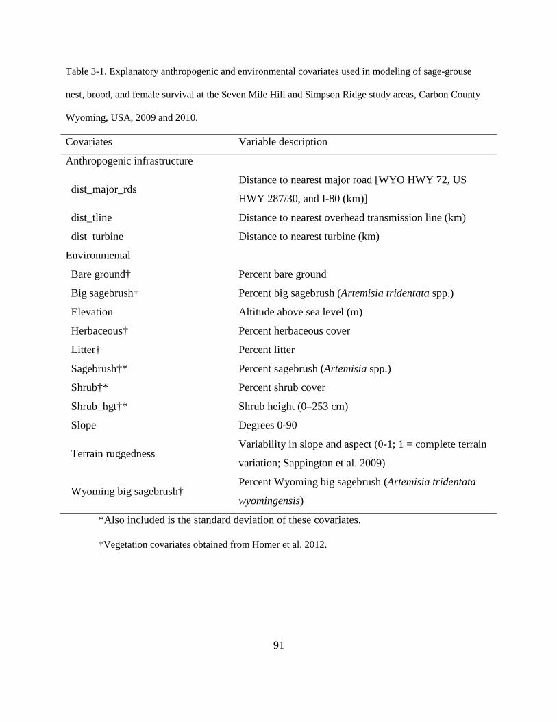
91
Table 3-1. Explanatory anthropogenic and environmental covariates used in modeling of sage-grouse
nest, brood, and female survival at the Seven Mile Hill and Simpson Ridge study areas, Carbon County
Wyoming, USA, 2009 and 2010.
Covariates Variable description
Anthropogenic infrastructure
dist_major_rds Distance to nearest major road [WYO HWY 72, US
HWY 287/30, and I-80 (km)]
dist_tline Distance to nearest overhead transmission line (km)
dist_turbine Distance to nearest turbine (km)
Environmental
Bare ground† Percent bare ground
Big sagebrush† Percent big sagebrush (Artemisia tridentata spp.)
Elevation Altitude above sea level (m)
Herbaceous† Percent herbaceous cover
Litter† Percent litter
Sagebrush†* Percent sagebrush (Artemisia spp.)
Shrub†* Percent shrub cover
Shrub_hgt†* Shrub height (0–253 cm)
Slope Degrees 0-90
Terrain ruggedness Variability in slope and aspect (0-1; 1 = complete terrain
variation; Sappington et al. 2009)
Wyoming big sagebrush† Percent Wyoming big sagebrush (Artemisia tridentata
wyomingensis)
*Also included is the standard deviation of these covariates.
†Vegetation covariates obtained from Homer et al. 2012.

92
Table 3-2. Model fit statistics for greater sage-grouse nest, brood, and survival at the Seven Mile Hill and
Simpson Ridge study areas, Carbon County, Wyoming, USA, 2009 and 2010. Models are listed
according to the model best fitting the data and ranked by (Δ AICc), the difference between the model
with the lowest Akaike’s Information Criterion for small samples (AICc) and the AICc for the current
model. The value of the maximized log-likelihood function (log[L]), the number of estimated parameters
(K), and Akaike’s weights (wi) for each model are also presented.
Model log[L] K AICc Δ AICc wi
Nest Survival
sd_shrub_hgt, dist_turbine, dist_tline -213.3 4 433.1 0.00 0.44
sd_shrub_hgt, dist_turbine -214.4 3 433.1 0.1 0.43
sd_shrub_hgt -216.7 2 435.6 2.5 0.13
null -218.7 1 437.4 4.3 0.05
Brood Survival
dist_turbine, terrain ruggedness, shrub -30.1 4 66.6 0.00 0.91
dist_turbine, terrain ruggedness -33.7 3 71.6 5.0 0.07
dist_turbine -36.6 2 75.4 8.8 0.01
null -38.3 1 76.5 10.0 0.01
Female Survival
dist_major_rds, dist_tline -187.3 3 378.9 0.00 0.55
dist_major_rds -188.6 2 379.3 0.37 0.45
null -189.7 1 379.4 0.69 0.28

93
Table 3-3. Relative risks of sage-grouse for each covariate or risk factor included in the top model for the
Seven Mile Hill and Simpson Ridge study areas in Carbon County, Wyoming, USA, 2009 and 2010.
Covariate Scale
(km) Estimate SE
Hazard Ratio
[exp(Estimate)]
Hazard Ratio 90% CI
Lower Upper
Nest Survival
sd_shrub_hgt 0.30 -0.16 -0.01 0.86 0.84 0.87
dist_turbine NA -0.06 -0.01 0.94 0.94 0.94
dist_tline NA 0.11 0.01 1.11 1.10 1.12
Brood Survival
dist_turbine NA -0.48 0.17 0.62 0.47 0.81
Terrain ruggedness 0.46 1.6 0.52 4.83 2.07 11.3
Shrub 1.0 1.1 0.43 3.03 1.49 6.16
Survival
dist_major_rds NA 0.19 0.02 1.21 1.16 1.25
dist_tline NA 0.09 0.01 1.09 1.09 1.10
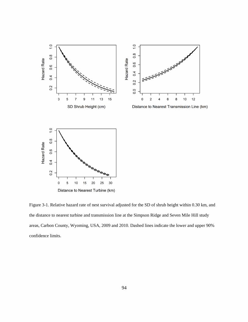
94
Figure 3-1. Relative hazard rate of nest survival adjusted for the SD of shrub height within 0.30 km, and
the distance to nearest turbine and transmission line at the Simpson Ridge and Seven Mile Hill study
areas, Carbon County, Wyoming, USA, 2009 and 2010. Dashed lines indicate the lower and upper 90%
confidence limits.
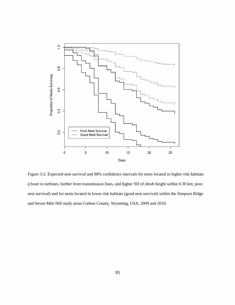
95
Figure 3-2. Expected nest survival and 90% confidence intervals for nests located in higher risk habitats
(closer to turbines, further from transmission lines, and higher SD of shrub height within 0.30 km; poor
nest survival) and for nests located in lower risk habitats (good nest survival) within the Simpson Ridge
and Seven Mile Hill study areas Carbon County, Wyoming, USA, 2009 and 2010.

96
Figure 3-3. Spatial variation in the predicted relative risk of sage-grouse nest failure (low – high) within
the Seven Mile Hill and Simpson Ridge study areas, Carbon County, Wyoming, USA, 2009 and 2010.

97
Figure 3-4. Relative hazard rate of brood survival adjusted for distance to nearest turbine, terrain
ruggedness, and percent shrub cover at the Simpson Ridge and Seven Mile Hill study areas, Carbon
County, Wyoming, USA, 2009 and 2010. Dashed lines indicate the lower and upper 90% confidence
limits.

98
Figure 3-5. Spatial variation in the predicted relative risk of sage-grouse brood failure (low – high) within
the Seven Mile Hill and Simpson Ridge study areas, Carbon County, Wyoming, USA, 2009 and 2010.

99
Figure 3-6. Relative hazard rate of female survival adjusted for the distance to nearest major road and
distance to nearest overhead transmission line at the Simpson Ridge and Seven Mile Hill study areas,
Carbon County, Wyoming, USA, 2009 and 2010. Dashed lines indicate the lower and upper 90%
confidence limits.

100
Figure 3-7. Spatial variation in the predicted relative risk of sage-grouse summer mortality (low – high)
within the Seven Mile Hill and Simpson Ridge study areas, Carbon County, Wyoming, USA, 2009 and
2010.

101
CHAPTER 4
Greater Sage-Grouse Male Lek Attendance Relative
to Wind Energy Development
In the format for manuscript submittal to the Journal of Wildlife Management
ABSTRACT
Trends in greater sage-grouse (Centrocercus urophasianus; hereafter, sage-grouse) population
abundance are typically indexed through lek counts documenting peak male attendance.
Monitoring male lek attendance can provide insight into the viability of sage-grouse populations.
Lek counts have been used to assess changes in male attendance rates and male recruitment at
leks impacted by anthropogenic features. Impacts to male lek attendance have been documented
at leks located in close proximity to oil and gas development. Furthermore, it has been
documented that there is a time lag of 2–10 years when measurable affects can be detected at
leks impacted by oil and gas development. It is unknown whether the same time lags or degree of
impact will occur at leks located in close proximity to wind energy development. My study
question focused on whether leks that were spatially proximate to wind energy infrastructure had
greater declines in male lek attendance from pre-development to 4 years post development of a
wind energy facility. I used a before-after-control-impact study design to assess male lek
attendance. Aerial surveys were flown to identify any unknown leks. In addition, 3 lek counts
were conducted at each occupied lek identified during the breeding season to determine the peak
number of males attending each lek. First, I used ratio of means of lek counts to investigate
differences among lek attendance pre and post development of the wind energy facility. Then, I
further investigated the changes in lek attendance pre and post development by calculating a
disturbance metric for each lek and regressing this metric with male lek attendance using linear

102
mixed effects models. Leks located within wind energy development experienced a significant
decline in male lek attendance from pre development to 4 years post development. However, leks
located outside of the wind energy development experienced similar significant declines. The top
model derived from the mixed effects linear model included one fixed term (year) and one
random component, the effect of individual leks. Leks that were influenced more by wind energy
development experienced similar declines as leks with no influence from pre development to 4
years post development. The significant decline in male lek attendance from 1 year pre
development to 4 years post development cannot solely be attributed to the presence of the wind
energy facility. Impacts from the wind energy facility may not be initially realized due to the
time lags associated with sage-grouse breeding populations. More than 4 years of post
development monitoring and multiple sites may be necessary to adequately assess greater sage-
grouse breeding response to wind energy development.
INTRODUCTION
Trends in sage-grouse population abundance are typically indexed through lek counts (Beck and
Braun 1980, Connelly and Braun 1997, Walsh et al. 2004). While the use of telemetry is the best
method to determine population demographic rates, lek counts provide a good index of breeding
population levels and in many cases long-term data sets are available for trend analysis
(Connelly and Braun 1997, Connelly et al. 2000a). Multiple studies have used lek counts to
provide information on sage-grouse breeding populations in response to disturbances including
prescribed burning (Connelly et al. 2000b) and oil and gas development (Holloran 2005, Walker
et al. 2007, Harju et al. 2010, Holloran et al. 2010).
The purpose of my study was to investigate the effect of wind energy infrastructure on
sage-grouse peak male lek attendance. Peak male lek attendance was defined as the highest

103
number of males attending each lek during any of the 3 counts initiated during the breeding
season. I used a before-after-control-impact study design (BACI) to evaluate the impacts of wind
turbines on male lek attendance (Green 1979, Morrison et al. 2008). BACI study designs consist
of knowing what type of impact will occur, when and where it will occur, and having the ability
to collect data prior to the impact (Green 1979) at the impacted site and a geographically similar
site that remains unaffected (control). I employed this study design to evaluate whether the
newly constructed wind turbines reduced male lek attendance at leks located near the facility
within 4 years of development. The objectives of this chapter were to (1) estimate a trend in peak
male attendance between leks with varying proximity to turbines pre and post-construction of the
Seven Mile Hill wind energy facility, and (2) compare those trend(s) to peak male attendance at
Simpson Ridge (control site).
STUDY AREA
The study area used in this chapter is consistent with the first 3 chapters of my thesis. Sage-
grouse leks located south of U.S. Highway 30/287 were within the SR study area and leks
located north of U.S. Highway 30/287 were within the SMH study area.
METHODS
Field Methods
To investigate the effect of wind energy infrastructure on the sage-grouse population, I
determined the distribution and number of males at active leks throughout the SMH (n = 5) and
SR (n = 9) study areas. I obtained the locations of known historic and existing sage-grouse leks
within 6.4 km (twice the distance of non-disturbance around leks suggested by Connelly et al
2000a) of the proposed SRWRA located in the SR and the SMH project areas from the
Wyoming Game and Fish Department (WGFD) lek database. Because it is important to detect all

104
leks when comparing lek counts to population trends (Walsh 2004), lek searches, following the
methodology outlined by WGFD (Christiansen 2007), were conducted during the 2009 lekking
period to detect any unknown leks within both study areas. Aerial surveys were conducted from
fixed-wing aircraft flying parallel transects designed to provide full coverage of both project
areas. These surveys were conducted during the peak of the lekking season from early April
through early May. All mapped historic and existing leks were flown to check for occupancy in
spring 2009. I conducted surveys from one-half hour before sunrise to one-half hour after sunrise
(Patterson 1952) during optimal weather conditions. Aerial flight transects were oriented north-
south and were separated by approximately 1.0 km. Transects were flown at a height of 91 to
137 m above ground level at an approximate speed of 161 kph. I recorded GPS coordinates and
the approximate numbers of grouse observed at all located leks. In addition, I obtained lek
locations and counts within 18 km (the furthest distance of a lek from the SMH turbines within
SMH and SR study areas) of SR and SMH study area because SR may not be an adequate
control for SMH because of its close proximity to SMH turbines. In addition, the area
encompassing an 18-km radius was selected by Johnson et al. (2011) to evaluate the influence of
environmental and anthropogenic features around sage-grouse leks because Connelly et al.
(2000a) recommended this distance around leks to manage for migratory sage-grouse
populations. These 22 leks were considered as the regional population (REG).
Ground surveys were conducted from 2008 to 2012 to count sage-grouse on identified
leks within SMH and SR. Lek counts for the regional leks were obtained from WGFD and only
included 2008 to 2011. Each active lek located during aerial surveys and known historic lek
locations in the survey area were visited 3 times each spring to count the number of sage-grouse
using the lek. Ground surveys were spaced a minimum of 7 days apart and occurred during the

105
lekking period (WGFD 2003). Counts were conducted for a 15–30 minute period in the early
morning when the lek was most active. I collected data on the maximum number of birds
counted by sex (males, females, unknown), date, time period of observation, and weather
information (temperature, wind speed and direction, cloud cover, precipitation; WGFD 2003).
Analytical Methods.—Because data were collected at each lek each year, I first estimated
the difference in the ratio of means of the peak male lek attendance between 2008 to 2009, 2008
to 2010, 2008 to 2011, and 2008 to 2012 within both study areas using a 500 iteration
bootstrapping technique where I sampled counts with replacement from each lek during each
year and calculated the ratio of means between the study areas and years. I calculated SE and
90% CI from the SD of the 500 bootstrap iterations. A statistically significant difference (alpha =
0.10; 90% confidence interval [CI] not including 0.0) between pre-construction (2008) and any
of the 4 years post-construction of the SMH facility indicated a change in the mean lek
attendance and warranted further investigation.
If there was statistically significant difference between any of the study areas then a more
complicated linear mixed-effects analysis (Henderson 1950, Goldberger 1962, McLean 1991,
Blickley et al. 2012) was used to investigate relationships between lek attendance and
disturbance metrics. Mixed models have both fixed and random effects. Fixed effects are
identical or constant for all groups (leks) in a population, and random effects are allowed to
differ from group to group (Gelman 2005). Random effects assume some type of relationship
within a group exists, and in this case we assumed a relationship within individual leks across
years. I used the following linear mixed model:
𝑅𝑖𝑗 = 𝛽0 + 𝛽1𝑋𝑖 + 𝛽2𝑌𝑒𝑎𝑟𝑗 + 𝜔𝑖 + 𝜀𝑖𝑗 ,

106
where 𝑅𝑖𝑗 was the attendance count values for each lek i (i=1,…,14) in year j (2008 = 1, 2009 =
2, 2010 = 3, 2011 = 4, and 2012 = 5), 𝑋𝑖 was a disturbance covariate measured at lek i, 𝑌𝑒𝑎𝑟𝑗
was the effect of year j, 𝜔𝑖 was a random lek effect, 𝜀𝑖𝑗 were error terms for each lek and year
assumed to be normally distributed, and 𝛽0(intercept), 𝛽1, and 𝛽2 were fixed-effect coefficients
to be estimated.
Fixed-effects (covariates) considered in my analysis included 5 disturbance metrics,
which included distance to nearest turbine and the proportion of turbines that overlapped each
lek. The distance to nearest turbine was the distance from the center of the lek to the nearest
turbine (km). I also included 4 different decay functions (-exp[distance]/decay distance)
representing various decay distances from turbines (i.e. 1.5, 5.0, 10, 15 km). The proportion of
overlapping turbines was calculated by buffering each lek by 3.2 km, which is the suggested
management area around each lek (Connelly et al. 2000a, Walker et al. 2007). I then buffered the
individual turbines with their access roads by varying sizes to evaluate various disturbance
proportions. These buffer sizes ranged from 0.60 km to 5.0 km and were determined from studies
where sage-grouse leks have been impacted by energy development (Table 4-1). The resulting
overlapping area(s) were used as covariates to estimate male lek attendance trends. I also
included a categorical covariate identifying each study area (1 = SMH and 0 = SR).
In addition to fixed effects, I also included a random effect in the mixed model. Peak
male lek attendance varied between leks located within both study areas. Subsequently, male lek
attendance over the 4-year period was more likely to be related within individual leks than
between leks. For example, lek attendance might consistently be 10–20 males at a lek for a span
of 5 to 10 years and another lek might consistently have around 75–100 males attending that lek

107
over the same time frame. To account for this pseudo-replication (Zuur et al. 2009), I considered
individual leks as a random effect in the mixed model.
To estimate the effects of turbines on male lek attendance, I followed a multiple step
process that included simple linear regression, mixed modeling, model selection, and goodness-
of-fit evaluations. I first used linear regression to investigate if there was an individual lek effect
on lek attendance. My response variable was the natural log (ln) of peak number of males
(hereafter count) and my explanatory variables was year interacting with the turbine disturbance
metric. Some leks recorded 0 males, subsequently I added 1 to each count (i.e., ln(count+1)). I
used residual plots to test for within lek-correlation and heterogeneity of the residuals (Zuur et al.
2009).
If within lek-correlation was present in the linear model further model development using
a random intercept would be warranted (Zurr et al. 2009). Model development followed a top-
down strategy (Diggle et al. 2002). I compared models using analysis of variance (ANOVA),
likelihood ratio tests, and Akaike’s information criterion corrected for small sample sizes (AICc;
Burham and Anderson 2002, Zuur et al. 2009). I first compared the linear model to a random
intercept model using ANOVA and likelihood ratios to determine whether a random intercept for
each lek was warranted and if further model development was needed (Zuur et al. 2009). If
results of the linear and random intercept model comparison were significantly different I
included lek as random effect in a mixed model (Zuur et al. 2009).
I used likelihood ratio tests and maximum likelihood estimation to compare the fixed
effects for the nested models. I used ML estimation to determine the optimal fixed structure
because models with different fixed effects fitted with REML cannot be compared on the basis
of their restricted likelihoods (Pinheiro and Bates 2000, Zuur et al. 2009). The models that

108
included the interaction of year and disturbance metric to models with no interactions were
compared. Models with and without the fixed effects were also compared to estimate the final
model. The final model parameters were estimated using REML (Zuur et al. 2009). Lastly, I
validated the final model by inspecting the residuals for equal scatter and homogeneity to ensure
a good model fit (Zuur et al. 2009). I also utilized a QQ-plot to assess the normality of the
residuals and the normality of the random effects (Zuur et al. 2009). Because SR may not be an
adequate control for SMH, I estimated mixed models with leks from all three study areas and
with only leks from SMH and SR to see if SR was an adequate control. If it was I would see
similar effects on lek attendance between the SR and REG leks.
RESULTS
Fourteen greater sage-grouse leks were observed during lek surveys in both study areas (5 within
SMH and 9 within SR during 2008, 2010, 2011, and 2012 (Table 4-2; Fig. 4-1). Two leks located
in SMH were not counted during 2009. During 2008 (pre-development of SMH wind energy
facility) the maximum number of male birds present at the occupied leks within the SMH study
area ranged from 18 males (Hanna Draw East 2) to 74 males (Missouri John), with a mean count
of 36 males per lek. During 2009, 2010, 2011, and 2012 the mean lek counts decreased to 34, 22,
8, and 9 males per lek, respectively at SMH. Similarly to SMH, occupied leks located within SR
had a mean count of 37 males/lek, ranging from 0 (Old Percy 2) to 111 males (Old Carbon 35-2)
in 2008. The mean male count peaked in 2009 (40 males/lek) then decreased to 23, 20, and 14
males per lek in 2010, 2011, and 2012, respectively (Table 4-2). I included 22 regional leks in
my analysis and the mean count ranged from 23 males/lek in 2008 to 7 males/lek in 2011.
Prior to construction in 2008, three leks were located within 1.6 km of the Seven Mile
Hill turbines, including the Missouri John, Pine Draw, and Commo 1 leks (Fig. 4-1). In 2008,

109
130 males were observed on all of these leks combined. In 2009, 103 males were counted on
these three leks (Table 4-2). There were 2 additional leks (Hanna Draw East 1 and 2) located
>3.2 km; however these leks were not surveyed in 2009 (Table 4-2; Fig. 4-1). In 2010, 2011, and
2012, leks within 3.2 km of the Seven Mile Hill turbines were surveyed. Data collected from
2009 through 2012 represent the first, second, third, and fourth sage-grouse breeding seasons,
respectively, after the wind-energy facility became operational. The three leks within 3.2 km
were located 0.58, 1.6, and 1.5 km from the nearest wind turbine (Fig. 4-1). The total number of
males counted on these three leks decreased from 130 the first year prior to construction (2008),
to 33 in 2012 with one lek becoming inactive (i.e., no males observed at the Pine Draw lek in
2012; Table 4-2).
The results from the ratio of means test indicated there was no significant difference from
2008 to 2012 between the three study areas. Regressing the ratio of means for each study area
against year indicated no significant difference between the slopes (SMH vs SR = 0.03; SE =
0.05; SMH vs REG = 0.04; SE = 0.07). I did however detect a significant difference in mean
male lek attendance from 2008 to 2011 between SMH and SR (Fig. 4-2). I further investigated
whether the addition of turbines to SMH had a greater impact on male lek attendance at leks with
closer proximity to turbines than leks farther from turbines by using linear mixed effects models.
Model Development
The residual plot for the linear regression model indicated unequal scatter of the residuals, thus
evidence of within-lek correlation in the data (Fig. 4-3). The likelihood ratio test indicated that
the random intercept model including lek as the random term was considerably better than the
linear model (L = 42.56, df = 1, P < 0.001). The optimal fixed structure included year interacting
with distance to nearest turbine (∆AIC = 0.402); however, this interaction was insignificant (β =

110
0.013; 90% CI: -0.003 –0.03). The final resulting model only included year as the fixed term.
The final model showed a significant year effect on male lek attendance. Male lek attendance
decreased on average by 25.6% (90% CI: 17.5–32.9%) every year from 2008 to 2012 within leks
located at SMH and SR. I observed similar trends when I incorporated the data from the regional
leks (n = 22). The interaction between year and distance to turbine was not significant (β = -
0.003; 90% CI: -0.011–0.006). Male lek attendance at the regional leks decreased on average by
31.4% (90% CI: 24.6–37.7%) every year from 2008 to 2011. Similar to the ratio of means
analysis there appeared to be no significant difference in male lek attendance from 1-yr pre
construction to 4 years post construction between the three study areas.
DISCUSSION
Ratio of means and linear mixed models were used to investigate the trends in peak male
attendance at leks impacted by wind turbines. I utilized a BACI study design to detect changes in
peak male attendance at leks prior to the construction and operation of the SMH wind energy
facility to 4 years post-development. I hypothesized that leks closer to turbines, or leks that had a
greater proportion of overlapping wind energy infrastructure, experienced a significant decrease
in male lek attendance from pre-construction to 4 years post construction.
Male lek attendance significantly decreased from 2008 to 2012; however, this decrease
could not be attributed to the degree of influence by wind turbines or the study area in which
each lek resided. Leks located in both study areas and regionally, significantly decreased from
2008 to 2012. The SR study area, which was not influenced by turbines, experienced similar
trends from 2008 to 2012 as did the leks located within SMH, the area influenced by wind
turbines.
111
Holloran (2005) assessed peak male lek attendance at 21 leks in southwestern Wyoming
over a time period that ranged from 1999 to 2004. Leks located within 5.0 km of oil and gas
development had significantly greater annual rates of decline than control leks (Holloran 2005).
Male lek attendance has also been shown to be negatively affected within 0.8, 3.2, and 4.8 km of
active well surfaces (Walker et al. 2007, Harju et al. 2010). In addition, leks impacted by oil and
gas development experience a time lag of when discernible affects on male lek attendance can be
measured (Walker et al. 2007, Doherty 2008, Harju et al. 2010). These time lags range from 2–
10 years (Harju et al. 2010) and 4 years (Doherty 2008) when effects of oil and gas development
can be measured on male lek attendance.
Although the results of my study indicate there was no difference in male lek attendance
between leks within and outside of wind energy development, the results from other studies
where leks have been impacted by oil and gas development indicate there is a time lag and
effects may not be realized until 2–10 years following development. There is only one
grouse/wind energy published study I am aware of that assessed male grouse lek attendance
relative to wind energy development. Black grouse (Tetrao tetrix) in Austria, were not impacted
by the wind energy facility the immediate year following construction, but did show considerable
declines 4 years after construction suggesting there may be a similar time lag to wind
development as oil and gas development in grouse (Zeiler and Grünschachner-Berger 2009). In
addition, a review of unpublished studies investigating the impacts to male lek attendance from
wind energy development indicated that prairie grouse may continue to use habitats near wind
energy developments and may experience similar time lags as oil and gas development (Johnson
and Stephens 2011). Further monitoring and inventorying of these leks will be necessary to
identify any long-term population trends (Fedy and Aldridge 2011).
112
LITERATURE CITED
Beck, T. D. I., C. E. Braun. 1980. The strutting ground count: variation, traditionalism,
management needs. Proceedings of the Western Association of Fish and Wildlife
Agencies 60:558–566.
Blickley, J. L., D. Blackwood, and G. L. Patricelli. 2012. Experimental evidence for the effects
fo chronic anthropogenic noise on abundance of greater sage-grouse at leks. Conservation
Biology 26:461-471.
Burnham K. P and D. R. Anderson. 2002. Model selection and multimodel Inference: a practical
information-theoretic approach: Second edition. Springer-Verlag, New York, New York,
USA.
Christiansen, T. 2007. Chapter 12: Sage Grouse (Centrocercus urophasianus). Pages 12-11 to
12-51 In Handbook of Biological Techniques. Third edition. S. A. Tessmann, edition.
Wyoming Game and Fish Department, Cheyenne, Wyoming, USA.
Connelly J. W., K. P. Reese, R. A. Fischer, and W. L. Wakkinen. 2000b. Response of a sage-
grouse breeding population to fire in southeastern Idaho. Wildlife Biology 28:90–96.
Connelly, J. W. and C. E. Braun. 1997. Long-term changes in sage-grouse Centrocercus
urophasianus populations in western North America. Wildlife Biology 3:123–128.
Connelly, J. W., M.A. Schroeder, A. R. Sands, and C. E. Braun. 2000a. Guidelines to manage
sage grouse populations and their habitats. Wildlife Society Bulletin 28:967−985.
Diggle, P. J., P. Heagerty, K. Y. Liang, and S. L. Zeger. 2002. The analysis of longitudinal data.
Second Edition. Oxford University Press, Oxford, England.

113
Doherty, K. 2008. Sage-grouse and energy development: Integrating science with conservation
planning to reduce impacts. Dissertation, University of Montana, Missoula, Montana,
USA.
Fedy, B. C., and C. L. Aldridge. 2011. The importance of within-year repeated counts and the
influence of scale on long-term monitoring of sage-grouse. Journal of Wildlife
Management 75:1022-1033.
Gelman, A. (2005). Analysis of varianace - why it is more important than ever. The Annals of
Statistics 33:1-53.
Goldberger, A. S. 1962. Best linear unbiased prediction in generalized linear regression model.
Journal of American Statistical Association 57:369-375.
Green, R. H. 1979. Sampling design and statistical methods for environmental biologists. Wiley
and Sons, New York, New York, USA.
Harju, S. M., M. R. Dzialak, R. C. Taylor, L. D. Hayden-Wing, J. B. Winstead. 2010. Thresholds
and time lags in effects of energy development on greater sage-grouse populations.
Journal of Wildlife Management 74:437–448.
Henderson, C. R. 1950. Estimation of genetic parameters. The Annals of Mathematical Statistics
21:309-310.
Holloran, M. J. 2005. Greater sage-grouse (Centrocercus urophasianus) population response to
natural gas field development in western Wyoming. Dissertation, University of
Wyoming, Laramie, USA.
Holloran, M. J., R. C. Kaiser, and W. A. Hubert. 2010. Yearling greater sage-grouse response to
energy development in Wyoming. Journal of Wildlife Management 74:65–72.
114
Johnson, D. H., M. J. Holloran, J. W. Connelly, S. E. Hanser, C. J. Amundson, and S. T. Knick.
2011. Influence of environmental and anthropogenic features on greater sage-grouse
populations, 1997–2007. Pages 407-450 in S. T. Knick and J. W. Connelly, editors.
Greater sage-grouse: ecology and conservation of a landscape species and its habitats.
Studies in Avian Biology Series. Volume 38. University of California Press, Berkeley,
California, USA.
Johnson, D. H. and S. E. Stephens. 2011. Windpower and biofuels: A geen dilemma for wildlife
conservation. Pages 131-157 in D. E. Naugle, editor. Wildlife Conservation in Western
North America. Island Press, Washington, DC, USA.
McLean, R. A., W. L. Sanders, and W. W. Stroup. 1991. A unified approach to mixed linear
models. The American Statistician 45:54-64.
Morrison, M. L., W.M. Block, M. D. Strickland, B. A. Collier, and M. J. Peterson. 2008.
Wildlife study design. Second Edition. Springer Press, New York, New York, USA.
Patterson, R. L. 1952. The sage grouse in Wyoming. Wyoming Game and Fish Commission and
Sage Books. Denver, Colorado, USA.
Pinheiro, J. and D. Bates. 2000. Mixed effects models in S and S-Plus. Springer-Verlag, New
York, New York, USA.
Walker, B. L., D. E. Naugle, and K. E. Doherty. 2007. Greater sage-grouse population response
to energy development and habitat loss. Journal of Wildlife Management 71:2644–2654.
Walsh, D. P., C. G. White, T. E. Remington, and D. C. Bowden. 2004. Evaluation of the lek-
count index for greater sage-grouse. Wildlife Society Bulletin 32:56–68.
Wyoming Game and Fish Department (WGFD). 2003. Wyoming greater sage-grouse
conservation plan. Wyoming Game and Fish Department, Cheyenne, Wyoming, USA.

115
Zeiler, H.P. and V. Grünschachner-Berger. 2009. Impact of wind power plants on black grouse,
Lyrurus tetrix in Alpine regions. Folia Zoologica 58:173-182.
Zuur, A. F., E. N. Ieno, N. J. Walker, A. A. Saveliev, and G. M. Smith. 2009. Mixed effects
models and extensions in ecology with R. Springer, New York, New York, USA.

116
Table 4-1. Disturbance metrics included in the mixed modeling procedure to determine potential extents
of impact from turbines to male lek attendance at leks located within the Seven Mile Hill and Simpson
Ridge study areas in Carbon County Wyoming, USA, 2008–2012. Metrics were derived from male
breeding use areas (0.60 km), identified management areas (3.2 km), or disturbance distances previously
determined from oil and gas development.
Variable Variable description
area_smh Nominal variable indicating study area the lek was located in
(1=SMH, 0=SR).
dist_turbine The distance to nearest turbine from each active lek within
both study areas (km).
sq_km600 The proportion of overlapping area within 0.60 km of
turbines and a 3.2 km buffer of each lek (CGSSC 2008).
sq_km1600
The proportion of overlapping area within 1.6. km of turbines
and a 3.2 km buffer of each lek (1.6 to 2 km, Harju et al.
2010)
sq_km3200 The proportion of overlapping area within 3.2 km of turbines
and a 3.2 km buffer of each lek (Connelly et al. 2000a)
sq_km5000 The proportion of overlapping area within 5.0 km of turbines
and a 3.2 km buffer of each lek (3-5 km Holloran 2005).
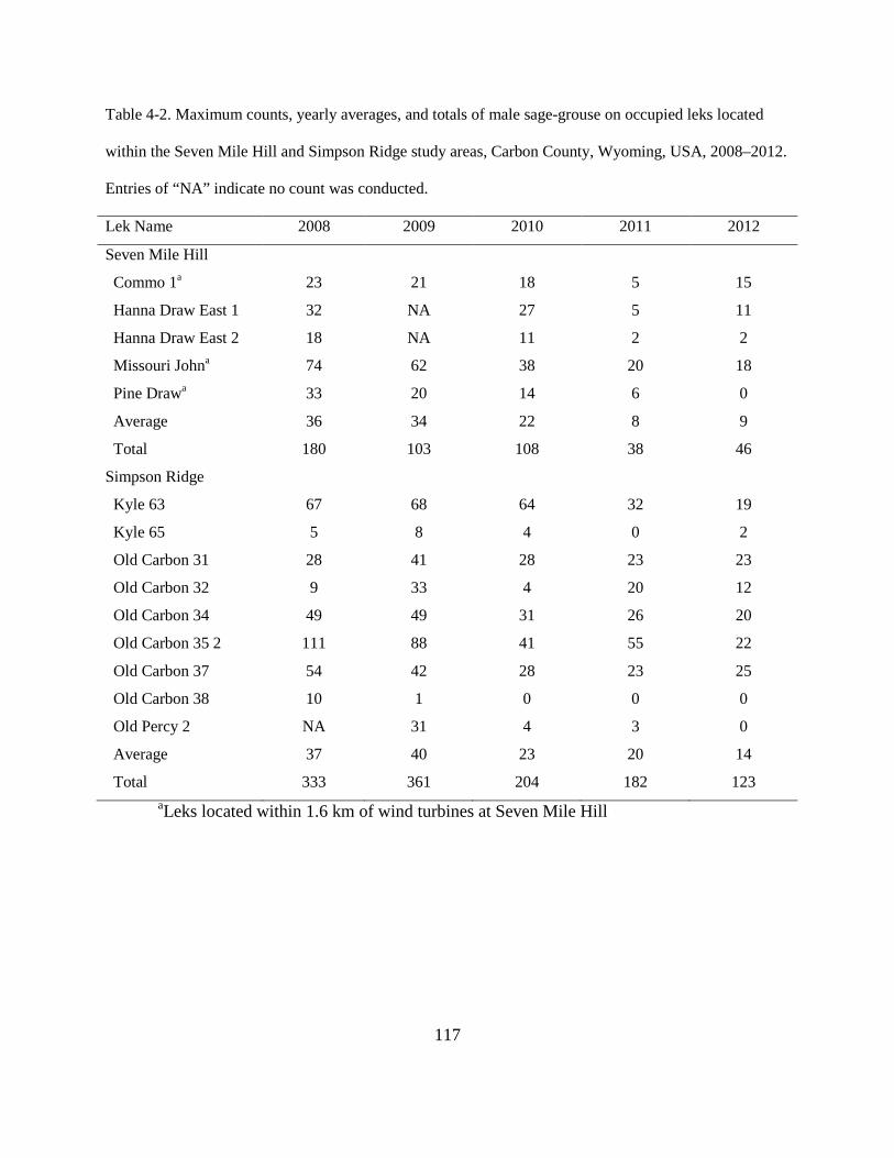
117
Table 4-2. Maximum counts, yearly averages, and totals of male sage-grouse on occupied leks located
within the Seven Mile Hill and Simpson Ridge study areas, Carbon County, Wyoming, USA, 2008–2012.
Entries of “NA” indicate no count was conducted.
Lek Name 2008 2009 2010 2011 2012
Seven Mile Hill
Commo 1a 23 21 18 5 15
Hanna Draw East 1 32 NA 27 5 11
Hanna Draw East 2 18 NA 11 2 2
Missouri Johna 74 62 38 20 18
Pine Drawa 33 20 14 6 0
Average 36 34 22 8 9
Total 180 103 108 38 46
Simpson Ridge
Kyle 63 67 68 64 32 19
Kyle 65 5 8 4 0 2
Old Carbon 31 28 41 28 23 23
Old Carbon 32 9 33 4 20 12
Old Carbon 34 49 49 31 26 20
Old Carbon 35 2 111 88 41 55 22
Old Carbon 37 54 42 28 23 25
Old Carbon 38 10 1 0 0 0
Old Percy 2 NA 31 4 3 0
Average 37 40 23 20 14
Total 333 361 204 182 123 aLeks located within 1.6 km of wind turbines at Seven Mile Hill
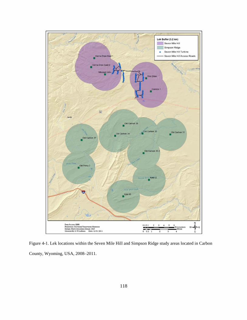
118
Figure 4-1. Lek locations within the Seven Mile Hill and Simpson Ridge study areas located in Carbon
County, Wyoming, USA, 2008–2011.
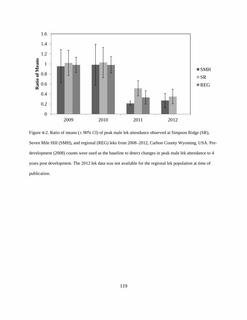
119
Figure 4-2. Ratio of means (± 90% CI) of peak male lek attendance observed at Simpson Ridge (SR),
Seven Mile Hill (SMH), and regional (REG) leks from 2008–2012, Carbon County Wyoming, USA. Pre-
development (2008) counts were used as the baseline to detect changes in peak male lek attendance to 4
years post development. The 2012 lek data was not available for the regional lek population at time of
publication.
0
0.2
0.4
0.6
0.8
1
1.2
1.4
1.6
2009 2010 2011 2012
Rat
io o
f Mea
ns
SMH SR REG
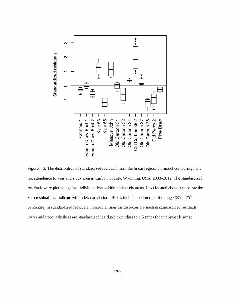
120
Figure 4-3. The distribution of standardized residuals from the linear regression model comparing male
lek attendance to year and study area in Carbon County, Wyoming, USA, 2008–2012. The standardized
residuals were plotted against individual leks within both study areas. Leks located above and below the
zero residual line indicate within lek correlation. Boxes include the interquartile range (25th–75th
percentile) in standardized residuals; horizontal lines inside boxes are median standardized residuals;
lower and upper whiskers are standardized residuals extending to 1.5 times the interquartile range.