To Vera Rae

3

Contents

1 Preliminaries 141.1 Elements of Linear Algebra . . . . . . . . . . . . . . . . . . . . . . . . . . . . 171.2 Hilbert Spaces and Dirac Notations . . . . . . . . . . . . . . . . . . . . . . . . 231.3 Hermitian and Unitary Operators; Projectors. . . . . . . . . . . . . . . . . . . 271.4 Postulates of Quantum Mechanics . . . . . . . . . . . . . . . . . . . . . . . . . 341.5 Quantum State Postulate . . . . . . . . . . . . . . . . . . . . . . . . . . . . . 361.6 Dynamics Postulate . . . . . . . . . . . . . . . . . . . . . . . . . . . . . . . . . 421.7 Measurement Postulate . . . . . . . . . . . . . . . . . . . . . . . . . . . . . . . 471.8 Linear Algebra and Systems Dynamics . . . . . . . . . . . . . . . . . . . . . . 501.9 Symmetry and Dynamic Evolution . . . . . . . . . . . . . . . . . . . . . . . . 521.10 Uncertainty Principle; Minimum Uncertainty States . . . . . . . . . . . . . . . 541.11 Pure and Mixed Quantum States . . . . . . . . . . . . . . . . . . . . . . . . . 551.12 Entanglement; Bell States . . . . . . . . . . . . . . . . . . . . . . . . . . . . . 571.13 Quantum Information . . . . . . . . . . . . . . . . . . . . . . . . . . . . . . . 591.14 Physical Realization of Quantum Information Processing Systems . . . . . . . 651.15 Universal Computers; The Circuit Model of Computation . . . . . . . . . . . . 681.16 Quantum Gates, Circuits, and Quantum Computers . . . . . . . . . . . . . . . 741.17 Universality of Quantum Gates; Solovay-Kitaev Theorem . . . . . . . . . . . . 791.18 Quantum Computational Models and Quantum Algorithms . . . . . . . . . . . 821.19 Deutsch, Deutsch-Jozsa, Bernstein-Vazirani, and Simon Oracles . . . . . . . . 891.20 Quantum Phase Estimation . . . . . . . . . . . . . . . . . . . . . . . . . . . . 961.21 Walsh-Hadamard and Quantum Fourier Transforms . . . . . . . . . . . . . . . 1021.22 Quantum Parallelism and Reversible Computing . . . . . . . . . . . . . . . . . 1071.23 Grover Search Algorithm . . . . . . . . . . . . . . . . . . . . . . . . . . . . . . 1111.24 Amplitude Amplification and Fixed-Point Quantum Search . . . . . . . . . . . 1231.25 Error Models and Quantum Algorithms . . . . . . . . . . . . . . . . . . . . . . 1301.26 History Notes . . . . . . . . . . . . . . . . . . . . . . . . . . . . . . . . . . . . 1321.27 Summary . . . . . . . . . . . . . . . . . . . . . . . . . . . . . . . . . . . . . . 1361.28 Exercises and Problems . . . . . . . . . . . . . . . . . . . . . . . . . . . . . . . 137

2 Measurements and Quantum Information 1422.1 Measurements and Physical Reality . . . . . . . . . . . . . . . . . . . . . . . . 1442.2 Copenhagen Interpretation of Quantum Mechanics . . . . . . . . . . . . . . . 1472.3 Mixed States and the Density Operator . . . . . . . . . . . . . . . . . . . . . . 1492.4 Purification of Mixed States . . . . . . . . . . . . . . . . . . . . . . . . . . . . 1562.5 Born Rule . . . . . . . . . . . . . . . . . . . . . . . . . . . . . . . . . . . . . . 1582.6 Measurement Operators . . . . . . . . . . . . . . . . . . . . . . . . . . . . . . 1592.7 Projective Measurements . . . . . . . . . . . . . . . . . . . . . . . . . . . . . . 1612.8 Positive Operator Valued Measures (POVM) . . . . . . . . . . . . . . . . . . . 1642.9 Neumark Theorem . . . . . . . . . . . . . . . . . . . . . . . . . . . . . . . . . 1672.10 Gleason Theorem . . . . . . . . . . . . . . . . . . . . . . . . . . . . . . . . . . 1682.11 Mixed Ensembles and their Time Evolution . . . . . . . . . . . . . . . . . . . 1722.12 Bipartite Systems; Schmidt Decomposition . . . . . . . . . . . . . . . . . . . . 174

4

2.13 Measurements of Bipartite Systems . . . . . . . . . . . . . . . . . . . . . . . . 1762.14 Operator-Sum (Kraus) Representation . . . . . . . . . . . . . . . . . . . . . . 1822.15 Entanglement; Monogamy of Entanglement . . . . . . . . . . . . . . . . . . . . 1852.16 Einstein-Podolski-Rosen (EPR) Thought Experiment . . . . . . . . . . . . . . 1892.17 Hidden Variables . . . . . . . . . . . . . . . . . . . . . . . . . . . . . . . . . . 1932.18 Bell and CHSH Inequalities . . . . . . . . . . . . . . . . . . . . . . . . . . . . 1992.19 Violation of Bell Inequality . . . . . . . . . . . . . . . . . . . . . . . . . . . . . 2022.20 Entanglement and Hidden Variables . . . . . . . . . . . . . . . . . . . . . . . . 2062.21 Quantum and Classical Correlations . . . . . . . . . . . . . . . . . . . . . . . . 2082.22 Measurements and Quantum Circuits . . . . . . . . . . . . . . . . . . . . . . . 2102.23 Measurements and Ancilla Qubits . . . . . . . . . . . . . . . . . . . . . . . . . 2142.24 Measurements and Distinguishability of Quantum States . . . . . . . . . . . . 2172.25 Measurements and an Axiomatic Quantum Theory . . . . . . . . . . . . . . . 2212.26 History Notes . . . . . . . . . . . . . . . . . . . . . . . . . . . . . . . . . . . . 2232.27 Summary and Further Readings . . . . . . . . . . . . . . . . . . . . . . . . . . 2252.28 Exercises and Problems . . . . . . . . . . . . . . . . . . . . . . . . . . . . . . . 228

3 Classical and Quantum Information Theory 2303.1 The Physical Support of Information . . . . . . . . . . . . . . . . . . . . . . . 2333.2 Entropy; Thermodynamic Entropy . . . . . . . . . . . . . . . . . . . . . . . . 2363.3 Shannon Entropy . . . . . . . . . . . . . . . . . . . . . . . . . . . . . . . . . . 2413.4 Shannon Source Coding . . . . . . . . . . . . . . . . . . . . . . . . . . . . . . 2513.5 Mutual Information; Relative Entropy . . . . . . . . . . . . . . . . . . . . . . 2553.6 Fano Inequality; Data Processing Inequality . . . . . . . . . . . . . . . . . . . 2593.7 Classical Information Transmission through Discrete Channels . . . . . . . . . 2613.8 Trace Distance and Fidelity . . . . . . . . . . . . . . . . . . . . . . . . . . . . 2673.9 von Neumann Entropy . . . . . . . . . . . . . . . . . . . . . . . . . . . . . . . 2693.10 Joint, Conditional, and Relative von Neumann Entropy . . . . . . . . . . . . . 2743.11 Trace Distance and Fidelity of Mixed Quantum States . . . . . . . . . . . . . 2753.12 Accessible Information in a Quantum Measurement; Holevo Bound . . . . . . 2823.13 No Broadcasting Theorem for General Mixed States . . . . . . . . . . . . . . . 2923.14 Schumacher Compression . . . . . . . . . . . . . . . . . . . . . . . . . . . . . . 2953.15 Quantum Channels . . . . . . . . . . . . . . . . . . . . . . . . . . . . . . . . . 2973.16 Quantum Erasure . . . . . . . . . . . . . . . . . . . . . . . . . . . . . . . . . . 3013.17 Classical Information Capacity of Noiseless Quantum Channels . . . . . . . . . 3063.18 Entropy Exchange, Entanglement Fidelity, and Coherent Information. . . . . . 3123.19 Quantum Fano and Data Processing Inequalities . . . . . . . . . . . . . . . . . 3183.20 Reversible Extraction of Classical Information from Quantum Information . . 3223.21 Noisy Quantum Channels . . . . . . . . . . . . . . . . . . . . . . . . . . . . . 3243.22 Holevo-Schumacher-Westmoreland Noisy Quantum Channel Encoding Theorem 3293.23 Capacity of Noisy Quantum Channels . . . . . . . . . . . . . . . . . . . . . . . 3343.24 Entanglement-Assisted Capacity of Quantum Channels . . . . . . . . . . . . . 3383.25 Additivity and Quantum Channel Capacity . . . . . . . . . . . . . . . . . . . 3423.26 Applications of Information Theory . . . . . . . . . . . . . . . . . . . . . . . . 3453.27 History Notes . . . . . . . . . . . . . . . . . . . . . . . . . . . . . . . . . . . . 347

5

3.28 Summary and Further Readings . . . . . . . . . . . . . . . . . . . . . . . . . . 3483.29 Exercises and Problems . . . . . . . . . . . . . . . . . . . . . . . . . . . . . . . 351

4 Classical Error Correcting Codes 3554.1 Informal Introduction to Error Detection and Error Correction . . . . . . . . . 3574.2 Block Codes. Decoding Policies . . . . . . . . . . . . . . . . . . . . . . . . . . 3594.3 Error Correcting and Detecting Capabilities of a Block Code . . . . . . . . . . 3634.4 Algebraic Structures and Coding Theory . . . . . . . . . . . . . . . . . . . . . 3664.5 Linear Codes . . . . . . . . . . . . . . . . . . . . . . . . . . . . . . . . . . . . 3754.6 Syndrome and Standard Array Decoding of Linear Codes . . . . . . . . . . . . 3834.7 Hamming, Singleton, Gilbert-Varshamov, and Plotkin Bounds . . . . . . . . . 3874.8 Hamming Codes . . . . . . . . . . . . . . . . . . . . . . . . . . . . . . . . . . . 3924.9 Proper Ordering, and the Fast Walsh-Hadamard Transform . . . . . . . . . . . 3944.10 Reed-Muller Codes . . . . . . . . . . . . . . . . . . . . . . . . . . . . . . . . . 4004.11 Cyclic Codes . . . . . . . . . . . . . . . . . . . . . . . . . . . . . . . . . . . . 4054.12 Encoding and Decoding Cyclic Codes . . . . . . . . . . . . . . . . . . . . . . . 4104.13 The Minimum Distance of a Cyclic Code; BCH Bound . . . . . . . . . . . . . 4214.14 Burst Errors. Interleaving . . . . . . . . . . . . . . . . . . . . . . . . . . . . . 4244.15 Reed-Solomon Codes . . . . . . . . . . . . . . . . . . . . . . . . . . . . . . . . 4274.16 Convolutional Codes . . . . . . . . . . . . . . . . . . . . . . . . . . . . . . . . 4384.17 Product Codes . . . . . . . . . . . . . . . . . . . . . . . . . . . . . . . . . . . 4454.18 Serially Concatenated Codes and Decoding Complexity . . . . . . . . . . . . . 4464.19 Parallel Concatenated Codes - Turbo Codes . . . . . . . . . . . . . . . . . . . 4494.20 History Notes . . . . . . . . . . . . . . . . . . . . . . . . . . . . . . . . . . . . 4534.21 Summary and Further Readings . . . . . . . . . . . . . . . . . . . . . . . . . . 4544.22 Exercises and Problems . . . . . . . . . . . . . . . . . . . . . . . . . . . . . . . 457

5 Quantum Error Correcting Codes 4615.1 Quantum Error Correction . . . . . . . . . . . . . . . . . . . . . . . . . . . . . 4635.2 A Necessary Condition for the Existence of a Quantum Code . . . . . . . . . . 4685.3 Quantum Hamming Bound . . . . . . . . . . . . . . . . . . . . . . . . . . . . . 4695.4 Scale-up and Slow-down . . . . . . . . . . . . . . . . . . . . . . . . . . . . . . 4705.5 A Repetitive Quantum Code for a Single Bit-flip Error . . . . . . . . . . . . . 4715.6 A Repetitive Quantum Code for a Single Phase-flip Error . . . . . . . . . . . . 4785.7 The Nine Qubit Error Correcting Code of Shor . . . . . . . . . . . . . . . . . 4835.8 The Seven Qubit Error Correcting Code of Steane . . . . . . . . . . . . . . . . 4855.9 An Inequality for Representations in Different Bases . . . . . . . . . . . . . . . 4905.10 Calderbank-Shor-Steane (CSS) Codes . . . . . . . . . . . . . . . . . . . . . . . 4945.11 The Pauli Group . . . . . . . . . . . . . . . . . . . . . . . . . . . . . . . . . . 5005.12 Stabilizer Codes . . . . . . . . . . . . . . . . . . . . . . . . . . . . . . . . . . . 5035.13 Stabilizers for Perfect Quantum Codes . . . . . . . . . . . . . . . . . . . . . . 5125.14 Quantum Restoration Circuits . . . . . . . . . . . . . . . . . . . . . . . . . . . 5155.15 Quantum Codes over GF (pk) . . . . . . . . . . . . . . . . . . . . . . . . . . . 5185.16 Quantum Reed-Solomon Codes . . . . . . . . . . . . . . . . . . . . . . . . . . 5215.17 Concatenated Quantum Codes . . . . . . . . . . . . . . . . . . . . . . . . . . . 527

6

5.18 Quantum Convolutional and Quantum Tail-Biting Codes . . . . . . . . . . . . 5285.19 Correction of Time-Correlated Quantum Errors . . . . . . . . . . . . . . . . . 5385.20 Quantum Error Correcting Codes as Subsystems . . . . . . . . . . . . . . . . . 5415.21 Bacon-Shor Code . . . . . . . . . . . . . . . . . . . . . . . . . . . . . . . . . . 5445.22 Operator Quantum Error Correction . . . . . . . . . . . . . . . . . . . . . . . 5495.23 Stabilizers for Operator Quantum Error Correction . . . . . . . . . . . . . . . 5535.24 Correction of Systematic Errors Based on Fixed-Point Quantum Search . . . . 5555.25 Reliable Quantum Gates and Quantum Error Correction . . . . . . . . . . . . 5575.26 History Notes . . . . . . . . . . . . . . . . . . . . . . . . . . . . . . . . . . . . 5605.27 Summary and Further Readings . . . . . . . . . . . . . . . . . . . . . . . . . . 5605.28 Exercises and Problems . . . . . . . . . . . . . . . . . . . . . . . . . . . . . . . 562

6 Physical Realization of Quantum Information Processing Systems 5656.1 Requirements for Physical Implementations of Quantum Computers . . . . . . 5676.2 Cold Ion Traps . . . . . . . . . . . . . . . . . . . . . . . . . . . . . . . . . . . 5736.3 First Experimental Demonstration of a Quantum Logic Gate . . . . . . . . . . 5836.4 Trapped Ions in Thermal Motion . . . . . . . . . . . . . . . . . . . . . . . . . 5886.5 Entanglement of Qubits in Ion Traps . . . . . . . . . . . . . . . . . . . . . . . 5906.6 Nuclear Magnetic Resonance - Ensemble Quantum Computing . . . . . . . . . 5966.7 Liquid-State NMR Quantum Computer . . . . . . . . . . . . . . . . . . . . . . 5986.8 NMR Implementation of Single-Qubit Gates . . . . . . . . . . . . . . . . . . . 6056.9 NMR Implementation of Two-Qubit Gates . . . . . . . . . . . . . . . . . . . . 6066.10 The First Generation NMR Computer . . . . . . . . . . . . . . . . . . . . . . 6126.11 Quantum Dots . . . . . . . . . . . . . . . . . . . . . . . . . . . . . . . . . . . 6146.12 Fabrication of Quantum Dots . . . . . . . . . . . . . . . . . . . . . . . . . . . 6216.13 Quantum Dot Electron Spins and Cavity QED . . . . . . . . . . . . . . . . . . 6246.14 Quantum Hall Effect . . . . . . . . . . . . . . . . . . . . . . . . . . . . . . . . 6286.15 Fractional Quantum Hall Effect . . . . . . . . . . . . . . . . . . . . . . . . . . 6316.16 Alternative Physical Realizations of Topological Quantum Computers . . . . . 6416.17 Photonic Qubits . . . . . . . . . . . . . . . . . . . . . . . . . . . . . . . . . . . 6436.18 Summary and Further Readings . . . . . . . . . . . . . . . . . . . . . . . . . . 649

7 Appendix. Observable Algebras and Channels 652

8 Glossary 688

7

“I want to know God’s thoughts... the rest are details. ” Albert Einstein.

Preface

A new discipline, Quantum Information Science, has emerged in the last two decades of thetwentieth century at the intersection of Physics, Mathematics, and Computer Science. Quan-tum Information Processing (QIP) is an application of Quantum Information Science whichcovers the transformation, storage, and transmission of quantum information; it represents arevolutionary approach to information processing

We have witnessed the development of microprocessors, high-speed optical communication,high-density storage technologies, followed by the widespread use of sensors, and more recentlymulti- and many-core processors and spintronics technology. We are now able to collecthumongous amounts of information, process the information at high speeds, transmit theinformation through high-bandwidth and low-latency channels, store it on digital media, andshare it using numerous applications built around the World Wide Web. Thus, the full cycleat the heart of information revolution was closed, Figure 1 [285], and this revolution becamea reality that profoundly affects our daily life.

Now, at the beginning of the twenty first century, information processing is facing newchallenges: heat dissipation, leakage, and other physical phenomena limit our ability to build

8

MICROPROCESSORS (1980s)

MULTI-CORE MICROPROCESSORS

(2000s)

WORLD WIDE WEB (1990s)

GOOGLE, YouTube (2000s)

FIBER OPTICS (1990s)

WIRELESS (2000s)

SENSORS

DIGITAL CAMERAS

(2000s)

COLLECT

PROCESSDISSEMINATE

COMMUNICATE

OPTICAL STORAGE

HIGH DENSITY SOLID-STATE

(1990s)

SPINTRONICS (2000s)

MILESTONES IN INFORMATION

PROCESSING

BOOLEAN ALGEBRA (1854)

DIGITAL COMPUTERS (1940s)

INFORMATION THEORY (1948)

Quantum Computing

Quantum Information Theory

STORE

Figure 1: Our ability to collect, process, store, communicate, and disseminate informationhas increased considerably during the last two decades of the twentieth century. 1980s wasthe decade of microprocessors; advances in solid state technologies allowed the increase of thenumber of transistors on a chip by three order of magnitude and a substantial reduction ofthe cost of a microprocessor. In 1990s we have seen major breakthroughs in optical storage,high density solid-state storage technologies, fiber optics communication, and the widespreadacceptance of the Word Wide Web. The first decade of the twenty first century is the decadeof sensors, rapid information dissemination, and multi-core microprocessors.

increasingly faster and, implicitly, increasingly smaller solid-state devices; it is very difficult toensure the security of our communication; we are overwhelmed by the volume of informationwe are bombarded with, and it is increasingly more difficult to extract useful informationfrom the vast ocean of information surrounding us.

Information, either classical or quantum, is physical; this is the mantra repeated through-out the book. Therefore, we must understand the physical processes that affect the state

9

of the systems used to carry information. The physical processes for the storage, transfor-mation, and transport of classical information are governed by the laws of classical Physicswhich limit our ability to process information increasingly faster using present day solid-statetechnologies. The speed of charge carriers in semiconductors is finite; to increase the speedof the device we have to pack the logic gates as tightly as possible.

The heat dissipated by a device increases with the clock rate to the power of 2 or 3,depending upon the solid-state technology. Heat removal is a hard problem for densely packeddevices; the heat produced by a solid-state device is proportional to the number of gatesthus, to the volume of the device. If we pack the gates into a sphere, the heat dissipatedis proportional to the volume of the sphere and can be removed through the surface of thesphere; while the amount of the heat increases as the cube of the radius, our ability to removeit only increases as the square of the radius of the sphere. We are thus limited in our abilityto increase the speed and density of classical circuits.

These facts provide a serious motivation to search for alternative physical realization ofcomputing and communication systems. Scientists are now exploring revolutionary means toovercoming the limitations of computing and communication systems based upon the laws ofclassical Physics. Quantum and biological information processing provide a glimpse of hopein overcoming some of the limitations we mentioned and could revolutionize computing andcommunication in the third millennium. DNA computing together with quantum computingand quantum communication are the most promising avenues explored nowadays. While asignificant progress has been made in understanding the properties of quantum information,fundamental questions regarding biological information are still waiting for answers. Forexample,how to explain the semantic aspect of biological information; how is informationfrom a damaged region of the brain recovered?

Quantum information is information stored as a property of a quantum system e.g., thepolarization of a photon, or the spin of an electron. Quantum information can be transmitted,stored, and processed following the laws of Quantum Mechanics. Several physical embodi-ments of quantum information are possible; for example, quantum communication involvesa source that supplies quantum systems in a given state, a noisy channel that “transports”the quantum system, and the recipient that receives and decodes the quantum information.The source could be a laser producing monochromatic photons, the channel could be an op-tical fiber and the recipient a photocell; the source could also be an ion trap controlled bylaser pulses, the channel a series of trapped ions, and the receiver a photo detector readingout the state of the ions via laser-induced fluorescence [276]. The diversity of the processesand technologies to process quantum information gives us hope that practical applications ofquantum information will emerge sooner rather than later.

The physical processes for photonic, ion-traps, quantum dots, NMR, and other quantumsystems are very different and could distract us from the goal of discovering the commonproperties of quantum information independent of its physical support. To study the proper-ties of quantum information we use an abstract model which captures the critical aspects ofquantum behavior; this model, Quantum Mechanics, describes the properties of physical sys-tems as entities in a finite-dimensional Hilbert space. Therefore, quantum information theoryrequires a basic understanding of Quantum Mechanics and familiarity with the mathematicalapparatus used by Quantum Mechanics and information theory.

Quantum information has special properties: the state of a quantum system cannot be

10

measured or copied without disturbing it; the quantum state of two systems can be entangled,the two-system ensemble has a definite state, though neither individual system has a welldefined state of its own; we cannot reliably distinguish non-orthogonal states of a quantumsystem. Charles Bennett noted that “Speaking metaphorically, quantum information is likethe information in a dream: attempting to describe your dream to someone else changes yourmemory of it, so you begin to forget the dream and remember only what you said about it.”[49].

The properties of quantum information are remarkable and could be exploited for infor-mation processing: in quantum computing systems an exponential increase in parallelismrequires only a linear increase in the amount of space needed thus, in principle, a quan-tum computer will be able to solve problems that cannot be solved with today’s computers;reversible quantum computers avoid logically irreversible operations and can, in principle, dis-sipate arbitrarily little energy for each logic operation. Quantum information theory allowsus to design algorithms for quantum key distribution and for quantum teleportation. Eaves-dropping on a quantum communication channel can be detected with very high probability.

Decoherence, the randomization of the internal state of a quantum computer due to interac-tions with the environment, is a major problem in quantum information processing; quantumcomputers rely on undisturbed evolution of quantum coherence. Quantum error correctionallows reliable communication over noisy quantum channels, provided that the channels arenot too noisy. We should caution the reader that the complexity of the circuits involvedin quantum error correction is far beyond today’s technological possibilities; a fault-tolerantimplementation of Shor’s quantum factoring algorithm would most likely require thousandsof physical qubits, at least two orders of magnitude more qubits than the systems reportedin the literature have been able to harness. It may be possible though to resort to techniqueswhich exploit the specific properties of individual physical realizations of quantum devicesto manage the complexity of the quantum circuits for fault-tolerant systems. Fault-tolerantquantum computing still requires many more years of research.

Quantum information processing involves several areas including: quantum algorithms,quantum complexity theory, quantum information theory, quantum error correcting codes,quantum cryptography, and quantum reliability. This book covers basic concepts in quantumcomputing, quantum information theory, and quantum error correcting codes.

Classical information theory is a mathematical model for the transfer, storage and process-ing of information based on the laws of classical Physics. In the late 1940s Claude Shannonproved that it is possible to reliably transmit information over noisy classical communicationchannels; this discovery triggered the search for classical error correcting codes and the firstcodes were discovered by Richard Hamming in the early 1950s. Error correction is a criticalcomponent of modern technologies for reliable transfer, storage and processing of classicalinformation. Quantum information theory (QIT) combines classical information theory withQuantum Mechanics to model information-related processes in quantum systems. The foun-dations of quantum information theory were established in the late 1980s by Charles Bennettand others and the interest in quantum information increased dramatically in mid 1990s afterPeter Shor and Andrew Steane showed that quantum error correction is feasible and, togetherwith Robert Calderbank, demonstrated that good quantum error correcting codes exist.

New discoveries add to the excitement of quantum information science: topological quan-tum computing proposed by Kitaev in 1997 and further developed by Friedman, Kitaev,

11

Larsen, and Wang has the potential to revolutionize fault-tolerance; in 2005 Grover discov-ered the fixed-point quantum search. In 2008 Smith and Yard showed that communicationis possible over zero capacity quantum channels and in 2009 Hastings provided an answer toone of the most important open question in quantum information theory showing that theminimum entropy output of a quantum communication channel is not additive. In 1999 Knill,Laflamme, and Viola reformulated quantum error correction and proposed to view quantumerror correcting codes as subsystems where the information resides in noiseless subspacesrather than considering a quantum code a subspace of a larger Hilbert space; in 2004 Kribs,Laflamme, and Poulin proposed a unified approach to quantum error correction and extendedthe concept of noiseless subsystems and their work led to the introduction of operator quan-tum error subsystems. These theoretical developments are mirrored by advances in quantumcommunication e.g., applications of Quantum Cryptography are close to commercialization.

The book organization is summarized in Figure 2; we first discuss classical concepts andthen, gradually, we move to the corresponding concepts for quantum information. We adoptedthis philosophy for several reasons. First, the classical concepts are easier to grasp. Naturalsciences develop increasingly more accurate and, at the same time, more complex models ofphysical reality; the level of abstraction makes it harder to develop the intuition behind theformalism and it is more difficult to master the mathematical apparatus the models are basedon. The second reason why we discuss first the classical concepts is because the targetedaudience for this book are not physicists familiar with Quantum Mechanics, but the largerpopulation of scientists, engineers, students, or ordinary people puzzled by the “strange”properties of quantum information. Some of them are familiar with the classical informationtheory concepts and with classical error correcting codes; for them the significant leap is totranspose their intuition, and knowledge to a different frame of reference.

We follow the same philosophy in the presentation of quantum algorithms; we analyzefirst quantum oracles, the easier to understand algorithms for “toy” problems proposed byDeutsch, Jozsa, Bernstein and Vazirani, and Simon followed by an in depth analysis of phaseestimation and of Grover search algorithm. The chapter covering information theory startswith the thermodynamic and Shannon entropy and classical channels and then we introducevon Neumann entropy and quantum channels. We discuss first linear codes and graduallymove to more sophisticated cyclic, convolutional, and other families of classical codes; sim-ilarly, we analyze first the Shor, Steane, and CSS quantum error correcting codes beforeintroducing stabilizer and subsystem codes. We hope that the numerous examples will facil-itate the understanding of the more abstract concepts introduced throughout the book andwill make the book accessible to a larger audience. Whenever possible we use the traditionalnotations in the literature or in the original papers which introduced the basic concepts. Thisrequired a careful selection of characters and fonts; for example, an 2n-dimensional Hilbertspace is denoted as H2n , Shannon entropy is H, the parity check matrix of a code is H theHadamard transform is H and the transfer matrix of a Hadamard gate is H.

The authors are indebted to several colleagues who have read the manuscript and havemade many constructive suggestions. Among them special thanks are due to Professors DanBurghelea from the Mathematics Department at Ohio State University, Eduardo Mucciolofrom the Physics Department, and Pawel Wocjan from the Computer Science Department atUniversity of Central Florida. Of course, the authors are responsible for the errors that, inspite of our efforts, may still be found in the text.

12

Mathematical Foundations

Chapter 1

Preliminaries

Quantum Mechanics

Concepts

Quantum Gates, Circuits,

Quantum Computers

Quantum Algorithms

von Neumann, POVM,

Measurements

Chapter 2

Measurements

Mixed States & Bipartite

Systems

Entanglement, EPR,

Bell & CSHS Inequalities

Measurements of

Quantum Circuits

Shannon Entropy and

Coding

Chapter 3

Information Theory

von Neumann Entropy

Noiseless Quantum

Channels

Noisy Quantum

Channels

Block Codes

Chapter 4

Classical ECC

Linear Codes. Bounds

Cyclic Codes

Convolutional, Product &

Concatenated Codes

Shor, Steane,

CSS Codes

Chapter 5

Quantum ECC

Stabilizer Codes

RS, Concatenated &

Convolutional Codes

Subsystem Codes

Requirements

Chapter 6

Physical Realization

Ion Traps

Nuclear Magnetic

Resonance

Quantum Dots

Anyons

Photons

Figure 2: Book organization at a glance.

The artwork was created by George Dima, a gifted artist, concertmaster of theBucharest Philharmonic and accomplished creator of computer-generated graphics (seehttp://picasaweb.google.com/degefe2008). We express our thanks to Patricia Osborne, GavinBecker, and the editorial staff from Elsevier for their constructive suggestions.

13

“No amount of experiments can ever prove me right; a single experiment can prove mewrong.” Albert Einstein.

1 Preliminaries

What is information? Carl Friederich von Weizsacker’s answer, information is what isunderstood, implies that information has a sender and a receiver who have a common under-standing of the representation and the means to convey information using some properties ofthe physical systems [447]. He adds, “Information has no absolute meaning; it exists relativelybetween two semantic levels” [448].

Once asked the question what is time, Richard Feynman answered: “time is what happenswhen nothing else happens.” Unfortunately, history did not record Feynman’s answer to thequestion “what is information” and thus we do not have a crisp, witty, and insightful answerto a question central to the 21st century science. Indeed, the questions what is informationand what is its relationship with the physical world become more important as we try to betterunderstand physical phenomena at quantum scale and the behavior of biological systems.

It is easy to understand why there is no simple answer to the question we posed at thevery beginning of this section; like matter and energy, information is a primitive concept thus,

14

it is rather difficult to rigorously define it. Informally, we can state that information abstractsproperties of and allows us to distinguish among objects/entities/phenomena/thoughts; infor-mation is a common denominator for the very diverse contents of our material and spiritualworld. There is a common expression of information as strings of bits, regardless of the ob-jects/entities/processes/thoughts it describes. Moreover, these bits are independent of theirphysical embodiment. Information can be expressed using pebbles on the beach, mechanicalrelays, electronic circuits, and even atomic and subatomic particles.

Classical information is information encoded to some property of a physical system obeyingthe laws of classical Physics. Classical information is transformed using logic operations.Classical gates implement logic operations and allow for processing of classical informationwith classical computing devices.

Quantum information is information encoded to some property of quantum particles andobeys the laws of Quantum Mechanics. Quantum information is transformed using quantumgates, the building blocks for quantum circuits, which, in turn, can be assembled to buildquantum computing and communication devices. The societal impact of information increasesif the physical embodiments of bits and gates become smaller and we need less energy toprocess, store, and transmit information. This justifies our interest in quantum information.

This book. This book covers topics in quantum computing, quantum information the-ory, and quantum error correction, three important areas of quantum information processing.Quantum information theory and quantum error correction build on the scope, concepts,methodology, and techniques developed in the context of their close relatives, classical infor-mation theory and classical error correcting codes. It seems natural to follow the historicalevolution of the concepts, and in this book, we first introduce the classical version of theconcepts and techniques which are often simpler and easier to grasp, and then discuss in de-tail the significant leaps forward necessary to apply the concepts and techniques to quantuminformation

Information theory is a mathematical model for transmission and manipulation of classicalinformation. Quantum information theory studies fundamental problems related to transmis-sion of quantum information over classical and quantum communication channels such as:the entropy of quantum systems, the capacity of classical and quantum channels, the effect ofthe noise, fidelity, and optimal information encoding. Quantum information theory promisesto lead to a deeper understanding of fundamental properties of nature and, at the same time,support new and exciting applications.

Error correcting codes allow us to detect and then correct errors during transmissionof classical information over classical channels and to build fault-tolerant computing andcommunication systems which obey the laws of classical Physics. Quantum error correctingcodes exploit the fundamental properties of quantum information investigated by quantuminformation theory and play an important role in the fault-tolerance of quantum computingand communication systems. Quantum error correcting codes are critical for the practical useof quantum computing and communication systems.

The first chapter of the book provides basic concepts from Mathematics, Quantum Me-chanics, and Computer Science necessary for understanding the properties of quantum infor-mation. Then we discuss the building blocks of a quantum computer, the quantum circuitsand quantum gates and survey some of the properties of quantum algorithms. Figure 3 pro-vides a structured view of the topics covered in this chapter: (1) the mathematical apparatus

15

Mathematical

FoundationsQuantum

Mechanics Quantum

Information

Processing

Quantum Oracles

- Phase Estimation

- W-HT and QFT

- Quantum Parallelism

& Reversibility

- Grover Search

- Amplitude Amplification

Figure 3: Chapter 1 at a glance.

used by Quantum Mechanics; (2) the fundamental ideas of Quantum Mechanics; (3) thecircuits and algorithms for quantum computing devices.

16

1.1 Elements of Linear Algebra

Familiarity with complex numbers, algebraic structures such as groups, Abelian groups, andfields [58] and linear algebra [170] is required to understand the mathematical formalism ofQuantum Mechanics. A review of algebraic structures used in coding theory is given in Section4.4; in this section we review concepts such as vector spaces, inner product, norm, distance,orthogonality, basis, orthonormal basis, dimension of a vector space, linear transformationand matrices, eigenvectors and eigenvalues, and trace.

A vector space is an algebraic structure consisting of:

1. An Abelian group (V, +) whose elements {vi} are called “vectors” and whose binaryoperation “+” is called addition;

2. A field F of numbers whose elements are called “scalars”; we restrict F to be either R

(the field of real numbers) or C (the field of complex numbers).

3. An operation called “multiplication with scalars” and denoted by “·”, which associatesto any scalar c ∈ F and vector vi ∈ V a new vector vj = c · vi ∈ V . F acts linearly onV : if a, b ∈ F and u, v ∈ V then a · (u + v) = a · u + a · v and (a + b) · u = a · u + b · u.

Assume that F ≡ C; it is easy to show that Cm×n, the set of all matrices A = [aij] with

entries aij ∈ C, 1 ≤ i ≤ n, 1 ≤ j ≤ m is a vector space where addition of two matricesA = [aij] and B = [bij] is defined as A + B = [aij + bij], the inverse with respect to additionof A = [aij] is −A = [−aij] and the identity element is E = [0].

A set B of vectors is called a basis in V if: (i) every vector v ∈ V can be expressed asa linear combination of vectors from B; (ii) the vectors in B are linearly independent. Thedimension of a vector space is the cardinality of B. We consider only finite-dimensional vectorspaces and in this case the cardinality is the number of elements of B. An n-dimensional vectorspace will be denoted as Vn.

An inner product in the vector space Vn over the field F is a mapping g : Vn × Vn �→ F

with several properties; ∀vi, vj, vk ∈ Vn and c ∈ F:

1. Obeys the addition rule in Vn:

g(vi + vj, vk) = g(vi, vk) + g(vj, vk) and g(vi, vj + vk) = g(vi, vj) + g(vi, vk).

2. Obeys the multiplication with a scalar rule in Vn:

g(c · vi, vj) = c × g(vi, vj) and g(vi, c · vj) = c∗ × g(vi, vj)

with c∗ the complex conjugate of c when F ≡ C.

3. Satisfies the following relations

g(vi, vj) = g(vj, vi) if F = R and g(vi, vj) = g∗(vj, vi) if F ≡ C.

17

4. The inner product is non-degenerate, g(vi, vi) ≥ 0 and g(vi, vi) = 0 if and only if vi = 0;

To simplify the notation the inner product g(vi, vj) will be written as 〈vi, vj〉 and we shall usethis notation from now on.

If an inner product in V is provided, then the norm || v || of the vector v ∈ Vn is thesquare root of the inner product of the vector with itself:

|| v ||=√

〈v, v〉.

The distance d(vi, vj) of two vectors vi, vj ∈ Vn is

d(vi, vj) =|| vi − vj ||=√

〈(vi − vj), (vi − vj)〉.

Two vectors, vi, vj ∈ Vn are orthogonal if

〈vi, vj〉 = 0.

The vectors of {b1, b2, . . . bn} ∈ Vn form an orthonormal basis if the inner product of anytwo of them is zero, 〈bibj〉 = 0, ∀(i, j) ∈ {1, n}, i �= j, and the norm of a vector is equal tounity, || bi ||= 〈bi, bi〉 = 1, ∀i ∈ {1, n}.

A linear operator A between two vector spaces V and W over the field F is any mappingfrom V to W , A : V �→ W , linear in its inputs

A

(∑i

civi

)=∑

i

ciA(vi).

The identity operator I maps v ∈ Vn to itself, I(v) = v. A linear transformation is a linearoperator with V = W .

The dual of a vector space V , denoted as V ∗, is the set of all scalar-valued linear mapsϕ : V �→ F. If we define the addition and scalar multiplications in V ∗ as

(ϕ + φ)(v) = ϕ(v) + φ(v) and (cϕ)(v) = cϕ(v)

with v ∈ V, c ∈ F and ϕ, φ ∈ V ∗, then the dual is also a vector space over the field F. If V isan n-dimensional vector space so is V ∗ and if the vectors {b1, b2, . . . , bj, . . . , bn} form a basisfor Vn then V ∗ is also an n-dimensional vector space and the vectors {b1, b2, . . . , bi, . . . , bn}defined by the property:

bi(bj) = δij =

{1 if i = j0 if i �= j

form a basis for V ∗. An inner product in V provides an isomorphism, i.e., an invertible linearoperator, A : V �→ V ∗, A(v)(w) = 〈v, w〉.

If we choose a basis B = {b1, b2, . . . , bn} then the linear transformation A is representedby an n × n matrix, A = [aij], 1 ≤ i, j ≤ n. Let the vectors v and w be

18

v =∑

i

vibi and w =∑

i

wibi

and w = Av. Then wi =∑n

j=1 aijvj which can be written as⎛⎜⎜⎜⎝

w1

w2...

wn

⎞⎟⎟⎟⎠ =

⎛⎜⎜⎜⎝

a11 a12 . . . a1n

a21 a22 . . . a2n...

......

...an1 an2 . . . ann

⎞⎟⎟⎟⎠⎛⎜⎜⎜⎝

v1

v2...

vn

⎞⎟⎟⎟⎠ .

with the right side of the equality representing the product of the n×n matrix whose elementsare aij’s with the n × 1 matrix whose elements are the vi’s.

Addition and multiplication of matrices satisfy standard algebraic laws:

A + B = B + A A + (B + C) = (A + B) + C A(B + C) = AB + ACA(BC) = (AB)C (A + B)C = AC + BC AI = IA = A

with I the identity matrix; In is an n × n matrix with main diagonal elements equal to oneand off-diagonal elements equal to zero. Non-zero matrices do not always have inverses andthe product of two matrices is in general noncommutative, AB �= BA.

The determinant of the n×n matrix A, det(A), is a number calculated from the elementsof matrix A; it vanishes if and only if the matrix represents a linear transformation which isnot one-to-one. The determinant can be written as a polynomial∣∣∣∣∣∣∣∣∣

a1 a2 a3 · · ·b1 b2 b3 · · ·c1 c2 c3 · · ·...

......

. . .

∣∣∣∣∣∣∣∣∣=∑ijk···

εijk··· aibjck · · ·

where (ijk....) a permutation of indices {1, 2, 3, . . .} and

εijk··· =

{1 for even permutations,

−1 for odd permutations.

}

The determinants of two n × n matrices A and B have the following property

det(AB) = det(A) det(B).

An eigenvector, v, of a linear transformation A is a non-zero vector such that

Av = λv.

The scalar λ is called an eigenvalue corresponding to the eigenvector v of A. The previousexpression can be also written as

Av = λIv.

Thus:

19

(A − λI)v = 0.

This equation can be transformed to a matrix equation by choosing a basis {bi}, for Vn. Withrespect to this basis v can be expressed as

v =∑

i

cibi.

Then,

(A − λI)∑

i

cibi = 0

where the coefficients must satisfy the equation∑i

(A − λI)i,jci = 0 for any fixed j.

A nontrivial solution exists only if the determinant

det(A − λ I) = 0.

The scalar λ for which that happens is an eigenvalue of A. This condition becomes:∣∣∣∣∣∣∣∣∣∣∣

(a11 − λ) a12 a13 · · · a1n

a21 (a22 − λ) a23 · · · a2n

a31 a32 (a33 − λ) · · · a3n...

......

. . .

an1 an2 an3 · · · (ann − λ)

∣∣∣∣∣∣∣∣∣∣∣= 0.

This is called the characteristic equation. The characteristic equation above is a polynomialof degree n in λ, where n is the dimension of the vector space. If F is either R or C thenthe polynomial has n possibly complex numbers as roots and by the “fundamental theoremof algebra” can be expressed as a product of linear factors:

(λ1 − λ)(λ2 − λ)(λ3 − λ) · · · (λn − λ) = 0.

If F = C then the n roots, λ1, λ2, λ3, . . . , λn are the eigenvalues of the operator and areindependent of the basis chosen to represent the operator as a matrix. If F = R then the realroots are eigenvalues.

If the characteristic equation has less than n distinct roots, there are multiple roots; theroot λ of multiplicity larger than one is said to be multiple. The multiplicity m of a rootλi is the number of times the factor (λi − λ) appears in the product above. For a multipleeigenvalue it is possible to have more than one eigenvector, all linearly independent and thecorresponding linear space is of dimension ≤ m.

If there are multiple eigenvalues of A and if for each multiple eigenvalue the multiplicitym is equal to the dimension d then it is possible to find a basis {b1, b2, . . . , bj, . . . , bn} for Asuch that each basis vector is an eigenvector of A:

20

Ab1 = λ1b1, Ab2 = λ2b2, Ab3 = λ3b3, . . . ,Abn = λnbn.

Then A with respect to the basis {b1, b2, . . . , bj, . . . , bn} can be expressed by the diagonalmatrix ⎛

⎜⎜⎜⎜⎜⎝

λ1 0 0 · · · 00 λ2 0 · · · 00 0 λ3 · · · 0...

......

. . .

0 0 0 · · · λn

⎞⎟⎟⎟⎟⎟⎠ .

Example. Let F = C and consider the matrix:

A =

(−1 2i−2i 2

)representing a linear transformation A : C �→ C

2. λ is an eigenvalue of A if the determinantof the matrix:

A − λI =

(−1 − λ 2i−2i 2 − λ

)is zero. The resulting characteristic polynomial

λ2 − λ − 6 = 0

has the roots λ1 = −2 and λ2 = 3. Hence, the eigenvectors of A satisfy one or the other ofthe following systems of equations:{

−x1 − 2iy1 = −2x1

2ix1 + 2y1 = −2y1or,

{−x2 − 2iy2 = 3x2

2ix2 + 2y2 = 3y2

where x1, x2 and y1, y2 represent the components corresponding to the basis vectors used torepresent matrix A.

The equations can be rewritten as{x1 − 2iy1 = 0ix1 + 2y1 = 0

or,

{2x2 + iy2 = 02ix2 − y2 = 0

Solving these systems of equations we obtain the eigenvectors (1,−12i) and (1, 2i). These

eigenvectors are not unique, (λ, 2iλ) are also eigenvectors. These eigenvectors can be used asa new basis and the transformed matrix A has a diagonal form:(

−2 00 3 − λ

)with respect to this basis. Now we review several important properties of square matriceswith elements from C useful for the proof of the proposition presented at the end of thissection.

21

The trace of a square matrix A = [aij] , 1 ≤ i, j ≤ n, aij ∈ C, is the sum of the elementson the main diagonal of A, tr(A) = a11 + a22 + . . . + ann. From this definition it is easy toprove several properties of the trace.

(i) The trace is a linear map. Given a scalar c ∈ R | C then tr(A + B) = tr(A) + tr(B) andtr(cA) = c tr(A). As a consequence, if A(t) is a matrix-valued function and d

dt[A(t)] denotes

the matrix whose entries are the derivatives of the entries of A(t) then

d

dt[tr(A(t))] = tr

(d

dt[A(t)]

).

(ii) The trace is invariant to transposition, tr(A) = tr(AT ). Indeed, the diagonal elements aii

of a square matrix A = [aij] are invariant to transposition.

(iii) The trace is not affected by the order of the matrices in a product of two matrices

tr(AB) = tr(BA).

If A = [aij] and B = [bij] , 1 ≤ i, j ≤ n, the diagonal elements of the products AB and BAare

∑ni=1 akibik and

∑ni=1 bkiaik; thus, tr(AB) = tr(BA). Consequently if U is a square n × n

matrix and it is invertible then

tr(U−1AU) = tr(A).

Given three n × n matrices A,B, and C we have tr(ABC) = tr(CAB) = tr(BCA). Anotherconsequence, if λ1, λ2, . . . λn are the eigenvalues of a square matrix A then

tr(A) =n∑

i=1

λi.

(iv) If A is a square matrix and A∗ is its complex conjugate, i.e., the entry of index ij is thecomplex conjugate of the entry ji, then

tr(A∗A) ≥ 0

Indeed,

tr(A∗A) =∑

1≤i,j≤n

aija∗ji =

∑1≤i,j≤n

| aij |2 .

It follows immediately thattr(A∗A) = 0 ⇔ A = 0.

From properties (i)-(iv) it follows that the set of n×n square matrices with elements fromC form a vector space with the inner product defined as

〈A,B〉 = tr(A∗B).

(v) The determinant and the trace are related

det(I + εA) = 1 + ε × tr(A) + o(ε2).

22

1.2 Hilbert Spaces and Dirac Notations

In this section we recast the linear algebra concepts using the formalism introduced by PaulDirac for Quantum Mechanics. Hilbert spaces could be of infinite dimension but we shall onlydiscuss finite-dimensional Hilbert spaces.

An n-dimensional Hilbert space Hn is an n-dimensional vector space over the field of com-plex numbers C, equipped with an inner product. In this case, the isomorphism A consideredabove, will be called Hermitian conjugation and denoted as ()†. The state of a physical systemwill be represented either as a vector in Hn and referred to as a ket vector or, equivalently,by its Hermitian conjugate and referred to as a bra vector. In this vector space distances andangles between vectors can be measured.

An example of a Hilbert space of dimension n is Cn when equipped with the inner product:

〈a, b〉 =n∑

i=1

aib∗i with a = (a1, a2, . . . an) and b = (b1, b2, . . . bn).

This Hilbert space has a canonical orthonormal base:

(1, 0, . . . , 0, 0), (0, 1, 0, . . . , 0, 0), . . . , (0, 0, . . . , 1, . . . , 0), . . . , (0, 0, . . . , 0, 1).

All n-dimensional Hilbert spaces are isomorphic with Cn by isomorphisms which identifythe inner products (isometries). More precisely, if v1, v2, . . . , vi, . . . , vn is an orthonormalbase, then the unique linear operator A : Hn �→ Cn defined by A(vi) = (0, 0, . . . , 1, . . . , 0)and extended linearly to all vi ∈ Hn is such an isometry. Conversely, for any isometryA : Hn �→ Cn, vi = A−1(0, 0, 0, . . . , 1, . . . , 0) provides an orthonormal basis in Hn. In viewof these remarks we can restrict ourselves to Cn as the “standard” representation of an n-dimensional Hilbert space, Hn.

Given two Hilbert spaces Hm and Hn over the same field F, their tensor product Hm ⊗Hn

is an (m × n)-dimensional Hilbert space, Hmn. If {e1, e2, . . . , em} is an orthonormal basis inHm and {f1, f2, . . . , fn} is an orthonormal basis in Hn then {ei ⊗ fj}, 1 ≤ i ≤ m, 1 ≤ j ≤ n,is an orthonormal basis in Hmn.

Quantum Mechanics uses a special notation for vectors; instead of the vector v we write | v〉and call it the ket vector representation of v; instead of the adjoint v† we write 〈v |, and callit the bra vector representation of v. With this convention the inner product (v, w) = (w†, v)can also be written as 〈w | v〉.

The canonical orthonormal basis of Cn can be expressed as ket vectors as

{| 0〉, | 1〉, . . . , | i〉, . . . , | n − 1〉},or, as bra vectors as

{〈0 |, 〈1 |, . . . , 〈i |, . . . , 〈n − 1 |}.We will also use the matrix representation of each ket vector | i〉 in this canonical represen-tation as a column vector with a 1 in the ith + 1 row and 0 in all the others. For example,

23

| 0〉 =

⎛⎜⎜⎜⎜⎜⎜⎜⎝

10...0...0

⎞⎟⎟⎟⎟⎟⎟⎟⎠

, | 1〉 =

⎛⎜⎜⎜⎜⎜⎜⎜⎝

01...0...0

⎞⎟⎟⎟⎟⎟⎟⎟⎠

, . . . , | i〉 =

⎛⎜⎜⎜⎜⎜⎜⎜⎝

00...1...0

⎞⎟⎟⎟⎟⎟⎟⎟⎠

, . . . , | n − 1〉 =

⎛⎜⎜⎜⎜⎜⎜⎜⎝

00...0...1

⎞⎟⎟⎟⎟⎟⎟⎟⎠

and the matrix representation of the bra vector 〈i | as a row vector with 1 in the ith + 1position and 0 in all the others:

〈0 |=(

1 0 . . . 0 . . . 0),

〈1 |=(

0 1 . . . 0 . . . 0),

...

〈i |=(

0 0 . . . 1 . . . 0),

...

〈n − 1 |=(

0 0 . . . 0 . . . 1).

We have:

〈i | j〉 = δi,j =

{0 if i �= j1 if i = j

0 ≤ (i, j) ≤ n − 1.

where δi,j is the Kronecker delta symbol.An n-dimensional ket | ψ〉 can be expressed in this basis as a linear combination of the

orthonormal basis ket vectors:

| ψ〉 = α0 | 0〉 + α1 | 1〉 + . . . + αi | i〉 + . . . + αn−1 | n − 1〉where α0, α1, . . . , αi, . . . , αn−1 are complex numbers.

The vector | ψ〉 can be expressed in different bases. For example, if n = 2 when the vectoris expressed in the basis | 0〉, | 1〉 as

| ψ〉 = α0 | 0〉 + α1 | 1〉then in a new basis {| x〉, | y〉} defined by

{| x〉 =1√2(| 0〉+ | 1〉), | y〉 =

1√2(| 0〉− | 1〉)}

the vector | ψ〉 is expressed as

| ψ〉 =1√2(α0 + α1) | x〉 +

1√2

(α0 − α1) | y〉.

For each ket vector | ψ〉 there is a dual, the bra vector denoted by 〈ψ |. As mentionedearlier the bra and ket vectors are related by Hermitian conjugation:

24

| ψ〉 = (〈ψ |)†, 〈ψ |= (| ψ〉)†.The bra vector 〈ψ | is expressed as a linear combination of the orthonormal bra vectors:

〈ψ |= α∗0〈0 | +α∗

1〈1 | + . . . + α∗i 〈i | + . . . + α∗

n−1〈n − 1 |where α∗

0, α∗1, . . . , α

∗i , . . . , α

∗n−1 are the complex conjugates of α0, α1, . . . , αi, . . . , αn−1.

In matrix representation, a ket vector is expressed as the column matrix:

| ψ〉 =

⎛⎜⎜⎜⎜⎜⎜⎜⎝

α0

α1...αi...

αn−1

⎞⎟⎟⎟⎟⎟⎟⎟⎠

and a dual bra vector is expressed as the row matrix:

〈ψ |=(

α∗0 α∗

1 . . . α∗i . . . α∗

n−1

).

Recall that the inner product of two vectors (| ψ〉, | ϕ〉) is a complex number. The innerproduct denoted as 〈ψ | ϕ〉 has the following properties:

1. The inner product of a vector with itself is a non-negative real number.Indeed:

〈ψ | ψ〉 =(

α∗0 α∗

1 α∗2 . . . α∗

n−1

)⎛⎜⎜⎜⎜⎜⎝

α0

α1

α2...

αn−1

⎞⎟⎟⎟⎟⎟⎠

=| α0 |2 + | α1 |2 + | α2 |2 + . . . + | αn−1 |2

with | αi |2, the square of the modulus of the complex number αi,

| αi |2= {�e(αi)}2 + {�m(αi)}2.

Thus, 〈ψ | ψ〉 ∈ R and:

〈ψ | ψ〉{

= 0 if 〈ψ |= (00 . . . 0)> 0 otherwise

2. Linearity. If | ψ〉, | ϕ〉, | ξ〉 ∈ Hn and (a, b, c) ∈ C

〈ψ | (c | ϕ〉) = c〈ψ | ϕ〉;

(a〈ψ | +b〈ϕ |) | ξ〉 = a〈ψ | ξ〉 + b〈ϕ | ξ〉;

25

〈ξ | (a | ψ〉 + b | ϕ〉) = a〈ξ | ψ〉 + b〈ξ | ϕ〉.3. Hermitian symmetry:

〈ψ | ϕ〉 = 〈ϕ | ψ〉∗.

Let A and B be two liner operators represented as m × n and p × q matrices:

A =

⎛⎜⎜⎜⎜⎜⎝

a11 a12 . . . a1n

a21 a22 . . . a2n

a31 a32 . . . a3n...

......

am1 am2 . . . amn

⎞⎟⎟⎟⎟⎟⎠ and B =

⎛⎜⎜⎜⎜⎜⎝

b11 b12 . . . b1q

b21 b22 . . . b2q

b31 b32 . . . b3q...

......

bp1 bp2 . . . bpq

⎞⎟⎟⎟⎟⎟⎠

then, their tensor product A ⊗ B is an mp × nq matrix defined as

A ⊗ B =

⎛⎜⎜⎜⎜⎜⎝

a11B a12B . . . a1nBa21B a22B . . . a2nBa31B a32B . . . a3nB...

......

am1B am2B . . . amnB

⎞⎟⎟⎟⎟⎟⎠ .

Here, aijB, 1 ≤ i ≤ m, 1 ≤ j ≤ n is a sub-matrix whose entries are the products ofaij and all the elements of matrix B. Consistent with this definition the tensor product oftwo-dimensional vectors (2 × 1 matrices), (a, b) and (c, d), is the four-dimensional vector (a4 × 1 matrix)

(ab

)⊗(

cd

)=

⎛⎜⎜⎝

acadbcbd

⎞⎟⎟⎠ .

Example. The tensor product of vectors (| 0〉, | 1〉) ∈ H2.

| 0〉 ⊗ | 1〉 =

(10

)⊗(

01

)=

⎛⎜⎜⎝

0100

⎞⎟⎟⎠ .

An m×n matrix obtained as a product of an m×1 matrix (a ket vector | ψ〉) and a 1×nmatrix (a bra vector 〈ϕ |) is sometimes called outer product. For example, let | ψ〉, | ϕ〉 ∈ H4

be

| ψ〉 = α0 | 0〉 + α1 | 1〉 + α2 | 2〉 + α3 | 3〉

| ϕ〉 = β0 | 0〉 + β1 | 1〉 + β2 | 2〉 + β3 | 3〉

26

Then the outer product | ψ〉〈ϕ | is the matrix

| ψ〉〈ϕ |=

⎛⎜⎜⎝

α0

α1

α2

α3

⎞⎟⎟⎠( β∗

0 β∗1 β∗

2 β∗3

)=

⎛⎜⎜⎝

α0β∗0 α0β

∗1 α0β

∗2 α0β

∗3

α1β∗0 α1β

∗1 α1β

∗2 α1β

∗3

α2β∗0 α2β

∗1 α2β

∗2 α2β

∗3

α3β∗0 α3β

∗1 α3β

∗2 α3β

∗3

⎞⎟⎟⎠ .

We conclude with the observation that in the case of Hilbert spaces any root of thecharacteristic polynomial of a linear transformation A is an eigenvalue. If an eigenvalue hasmultiplicity 1 the eigenvector is unique up to multiplication with a scalar but, if we insist thatthe eigenvector be unitary (of length 1), then the eigenvector is unique up to a phase factor.As we shall see in Sections 1.5, 1.6, and 1.7 vectors in Hilbert space represent the states ofa quantum system; the transformation of states and the measurements are represented bylinear operators.

1.3 Hermitian and Unitary Operators; Projectors.

A linear operator A maps vectors in a space Hn to vectors in the same space Hn. Giventhe vectors | ψ〉, | ϕ〉 ∈ Hn the transformation performed by the linear operator A can bedescribed as

| ϕ〉 = A | ψ〉.With respect to an orthonormal basis chosen once and for all, the linear operator A on Hn

can be represented by the matrix

A = [aij], with aij ∈ C, 1 ≤ i, j ≤ n.

The adjoint of a linear operator A is denoted A†. The matrix A† describing the adjoint

operator A† is the transpose conjugate matrix of A

A† = [a∗ji], 1 ≤ i, j ≤ n.

Throughout this book the term operator means linear operator and we shall use the termsoperator A and matrix A interchangeably. An operator acts on the left of a ket vector andon the right of a bra vector. Moreover,

[A | ϕ〉]† =| ϕ〉†A† = 〈ϕ | A†.

An operator A is normal if AA† = A†A. An operator A is Hermitian (self-adjoint) if

A = A†. Clearly, a Hermitian operator is normal. The sum of two Hermitian operatorsA = A† and B = B† is Hermitian

(A + B)† = A† + B† = A + B

while their product is not necessarily Hermitian. The necessary and sufficient condition forthe product of two Hermitian operators to be Hermitian is AB = BA or AB−BA = 0. Theexpression:

27

[A,B] = AB − BA

is called the commutator of A and B. Thus, the product of two Hermitian operators is aHermitian operator if and only if their commutator is equal to zero.

We now introduce a class of Hermitian operators of special interest in Quantum Mechanics;a projector, P, is a Hermitian operator with the property: P2 = P. The outer product of astate vector | ϕ〉 with itself is a projector: Pϕ =| ϕ〉〈ϕ |. Two projectors Pi, Pj are orthogonalif, for every state | ψ〉 ∈ Hn the following equality holds

PiPj | ψ〉 = 0

This condition is often written asPiPj = 0.

A set of orthogonal projectors {P0,P1,P2, . . .} is complete/exhaustive if∑i

Pi = I.

It it easy to see that

(Pϕ)† = (| ϕ〉〈ϕ |)† =| ϕ〉〈ϕ |= Pϕ.

If | ϕ〉 is normalized, 〈ϕ | ϕ〉 = 1, then P2ϕ = Pϕ.

(Pϕ)2 = (Pϕ)†(Pϕ) = (| ϕ〉〈ϕ |)(| ϕ〉〈ϕ |) =| ϕ〉〈ϕ |= Pϕ.

Properties of Hermitian operators. Hermitian operators enjoy a set of remarkableproperties; some of them, P1 - P5 are discussed next.

P1. The eigenvalues of a Hermitian operator in Hn are real.

Proof: We calculate the inner product 〈ψ | A | ψ〉 where λψ is the eigenvalue correspondingto the eigenvector | ψ〉 of A:

〈ψ | A | ψ〉 = 〈ψ | [A | ψ〉] = 〈ψ | [λψ | ψ〉] = λψ〈ψ | ψ〉If we take the adjoint of A | ψ〉 = λψ | ψ〉 and use the fact that A is Hermitian, A = A†, itfollows that 〈ψ | A = λ∗

ψ〈ψ |. We now rewrite the inner product:

〈ψ | A | ψ〉 = [〈ψ | A] | ψ〉 =[λ∗

ψ〈ψ |]| ψ〉 = λ∗

ψ〈ψ | ψ〉.It follows that

λψ〈ψ | ψ〉 = λ∗ψ〈ψ | ψ〉 =⇒ (λψ − λ∗

ψ)〈ψ | ψ〉 = 0, ∀ | ψ〉 ∈ Hn.

Since 〈ψ | ψ〉 �= 0, it follows that λψ = λ∗ψ thus, the eigenvalue λψ is a real number.

P2. Two eigenvectors | ψ〉 and | ϕ〉 of the Hermitian operator A with distinct eigenvalues,λψ �= λϕ are orthogonal, 〈ψ | ϕ〉 = 0.

28

Proof: We calculate the inner product 〈ψ | A | ϕ〉 and use the fact that λϕ is an eigenvalueof A corresponding to the eigenvector | ϕ〉 thus, A | ϕ〉 = λϕ | ϕ〉:

〈ψ | A | ϕ〉 = 〈ψ | [A | ϕ〉] = 〈ψ | [λϕ | ϕ〉] = λϕ〈ψ | ϕ〉.The eigenvalue λψ corresponds to the eigenvector | ψ〉 thus, A | ψ〉 = λψ | ψ〉. If we takethe adjoint of this expression and use the fact that A is Hermitian, A = A†, it follows that〈ψ | A = λ∗

ψ〈ψ |. We can now rewrite the inner product:

〈ψ | A | ϕ〉 = [〈ψ | A] | ϕ〉 =[λ∗

ψ〈ψ |]| ϕ〉 = λ∗

ψ〈ψ | ϕ〉.It follows that

λϕ〈ψ | ϕ〉 = λ∗ψ〈ψ | ϕ〉 ∀ λψ �= λϕ.

This is possible if and only if: 〈ψ | ϕ〉 = 0.

P3. For every Hermitian operator A there exists a basis of orthonormal eigenvectors suchthat the matrix A is diagonal in that basis and its diagonal elements are all the eigenvaluesof A.

Proof: Let | ψi〉, 1 ≤ i ≤ n, be an eigenvector of A and λi the corresponding eigenvalue. Ifthe eigenvalues are distinct, λi �= λj for i �= j, 1 ≤ i, j ≤ n, we construct the orthonormalbasis as follows: we select an eigenvector | ψj〉 from a subspace that is orthogonal to thesubspace spanned by (| ψ1〉, | ψ2〉, · · · , | ψi〉).

Then:

A =

⎛⎜⎜⎜⎜⎜⎝

λ1 0 0 · · ·0 λ2 0 · · ·0 0 λ3 · · ·...

......

. . .

λn

⎞⎟⎟⎟⎟⎟⎠

If the eigenvalues λj are degenerate (not distinct), then there are many bases of eigenvectorsthat diagonalize matrix A. If λ is an eigenvalue of multiplicity K > 1, the set of correspondingeigenvectors generate a subspace of dimension K, the eigenspace corresponding to that λ;the eigenspaces corresponding to different eigenvalues are orthogonal. Assume that λ is adegenerate eigenvalue and the corresponding eigenvectors are | ψλ1〉 and | ψλ2〉:

A | ψλ1〉 = λ | ψλ1〉 and A | ψλ2〉 = λ | ψλ2〉.Then, ∀a1, a2 ∈ C:

A(a1 | ψλ1〉 + a2 | ψλ2〉) = λ(a1 | ψλ1〉 + a2 | ψλ2〉).We can say that there is a whole subspace spanned by vectors | ψλ1〉 and | ψλ2〉, the elementsof which are eigenvectors of A with eigenvalues λ.

P4. The necessary and sufficient condition for two Hermitian operators, A1 and A2, tohave the same set of eigenvectors is that they commute with each other:

29

[A1,A2] = A1A2 − A2A1 = 0

P5. The eigenvectors of a projector operator, Pψ =| ψ〉〈ψ |, where 〈ψ | ψ〉 = 1, are eitherperpendicular to or collinear to the vector | ψ〉 and their eigenvalues are 0 and 1, respectively.

Proof: Assume | ϕ〉 is an eigenvector of Pψ corresponding to eigenvalue λ:

Pψ | ϕ〉 = λ | ϕ〉

or,| ψ〉〈ψ | ϕ〉 = λ | ϕ〉.

The inner product 〈ψ | ϕ〉 is a number γ

γ | ψ〉 = λ | ϕ〉

This implies that

λ = 0 if γ = 0, when | ψ〉 and | ϕ〉 are perpendicular

or,

λ = 1 if γ = 1, when | ψ〉 and | ϕ〉 are parallel and normalized.

An operator A is unitary if AnA†n = A†

nAn = In. Clearly, a unitary operator is normal.The product of unitary operators is unitary, but the sum is not; “product” in this case meanscomposition, not to be confused with tensor product.

A unitary operator A preserves the inner product, thus, it preserves the distance in aHilbert space. If | ψ1〉, | ψ2〉, | ϕ1〉, | ϕ2〉 ∈ Hn and | ϕ1〉 = A | ψ1〉 and | ϕ2〉 = A | ψ2〉 then:

〈ϕ1 | ϕ2〉 = 〈ψ1 | ψ2〉Indeed the inner product 〈ϕ1 | ϕ2〉 can be written as

〈ϕ1 | ϕ2〉 = [A | ψ1〉]†A | ψ2〉 = 〈ψ1 | A†A | ψ2〉 = 〈ψ1 | ψ2〉.It follows immediately that a unitary operator A preserves the norm of a vector:

[〈ϕ | A†] [A | ϕ〉] = 〈ϕ | [A†A] | ϕ〉 = 〈ϕ | ϕ〉If A is a unitary operator then we can undo its action, i.e., a unitary operator is invertibleand A−1 = A†.

Every normal operator has a complete set of orthonormal eigenvectors. If | ei〉 is aneigenvector (eigenstate) of the operator A and λi is the associated eigenvalue, then we canwrite:

A | ei〉 = λi | ei〉.The spectral decomposition of a normal operator A is

30

A =∑

i

λi Pi

with Pi =| ei〉〈ei | the projector corresponding to the eigenvector | ei〉.Proof: Note that (A + A†)/2 and (A − A†)/2i are Hermitian and commute. By P3 and P4there exists an orthonormal base {e1, e2, . . . , en} of eigenvectors simultaneously for (A+A†)/2and (A − A†)/2i. Hence they are also eigenvectors for

A =

(A + A†

2+ i

A − A†

2i

).

Let λ1, λ2, . . . λn be the eigenvalues corresponding to the eigenvectors {e1, e2, . . . , en}.

A =∑

i

λiPi with Pi =| ei〉〈ei | .

Indeed, both A and∑

i λiPi have the same matrix representation with respect to the base{e1, e2, . . . , en}.

Example. Choose an orthonormal basis in H2. Let A be a 2 × 2 matrix in this basis is

A =

(a11 a12

a21 a22

).

Calculate its eigenvalues λ1 and λ2, possibly equal. Find linearly independent solutions of thetwo linear equations:

A

(x1

y1

)= λ1

(x1

y1

)and A

(x2

y2

)= λ2

(x2

y2

).

Define

v1 =

⎛⎝ x1√

|x1|2+|y1|2y1√

|x1|2+|y1|2

⎞⎠ and v2 =

⎛⎝ x2√

|x2|2+|y2|2y2√

|x2|2+|y2|2

⎞⎠

The vectors | v1〉 and | v2〉 form another basis for A such that we can express for A as

A = λ1 | v1〉〈v1 | +λ2 | v2〉〈v2 | .

Now we introduce the concept of positive operators and define the square root and themodulus of a positive operator; then we describe the canonical decomposition of an invertibleoperator [355].

Positive operators. An operator V : Hn �→ Hn is a positive operator, V > 0, iff:

〈Vϕ | ϕ〉 > 0, ∀ | ϕ〉 ∈ Hn, | ϕ〉 �= 0.

The eigenvalues of a positive definite operator are real and positive.

31

An operator is positive semi-definite if ∀ | ϕ〉 �= 0 〈Vϕ | ϕ〉 = 〈ϕ | V | ϕ〉 ≥ 0; theeigenvalues of V are real and non-negative thus, trV ≥ 0. A positive semi-definite operatoris self-adjoint. If two positive operators commute then their product is a positive operator.

If V is a positive semi-definite operator there exists a unique positive semi-definite operatorQ such that Q2 = V denoted also by Q =

√V. Indeed, there exits an orthonormal base in Hn

consisting of eigenvectors of V; with respect to this basis V can be represented as a diagonalmatrix, diag (p1, p2, . . . pn). Since V is positive then pi ≥ 0, hence they have unambiguouslydefined positive square roots. Define:

Q =√

V to be represented by diag (√

p1,√

p2, . . . ,√

pn) .

The modulus of any operator V is defined as

| V |=√

V†V ≥ 0,

it is always positive. One can also consider√

V†V ≥ 0 but, unless V is normal, that is notthe same as

√(VV†) ≥ 0.

The operator Q is invertible if:

| Q || Q |−1= I

If an operator Q is invertible then it can be written as a product of a positive-definiteoperator, V, and a unitary operator, U:

Q = VU, with V =| Q |=√

QQ† and U = | Q |−1Q.

From definition it follows immediately that V is positive as the modulus of Q. To check thatU is unitary, observe that | Q | and | Q |−1 are self-adjoint hence | Q |†=| Q | .Then we have

UU† =| Q |−1 QQ†(| Q |−1)† =| Q |−1 QQ† | Q |−1=| Q |−1| Q || Q || Q |−1= I.

To prove that this decomposition is unique we assume that

Q = V1U1 and Q = V2U2.

Then, we use the fact that U1 and U2 are unitary, U1U†1 = U2U

†2 = I, to get:

QQ† = [V1U1] [V1U1]† = V1U1U

†1V

†1 = V1V

†1 = V2

1.

and

QQ† = [V2U2] [V2U2]† = V2U2U

†2V

†2 = V2V

†2 = V2

2

It follows that V1 = V2 and immediately that U1 = U2.

Another useful property of a positive operator V regards the trace of the product of Vand a unitary operator U. The maximum with respect to U of the trace of the product VUis

32

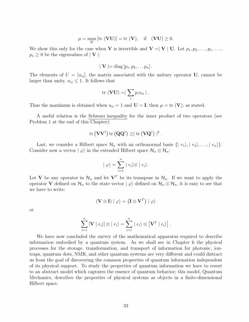
μ = maxU

[tr (VU)] = tr (V), if (VU) ≥ 0.

We show this only for the case when V is invertible and V =| V | U. Let p1, p2, . . . , pi, . . . ,pn ≥ 0 be the eigenvalues of | V |:

| V |= diag [p1, p2, . . . pn] .

The elements of U = [uij], the matrix associated with the unitary operator U, cannot belarger than unity, uij ≤ 1. It follows that

tr (VU) =|∑

i

piuii | .

Thus the maximum is obtained when uii = 1 and U = I; then μ = tr (V), as stated.

A useful relation is the Schwarz inequality for the inner product of two operators (seeProblem 1 at the end of this Chapter):

tr(VV†) tr

(QQ†) ≥| tr

(VQ†) |2 .

Last, we consider a Hilbert space Hn with an orthonormal basis {| e1〉, | e2〉, . . . , | en〉}.Consider now a vector | ϕ〉 in the extended Hilbert space Hn ⊗Hn:

| ϕ〉 =n∑

i=1

| ei〉⊗ | ei〉.

Let V be any operator in Hn and let VT be its transpose in Hn. If we want to apply theoperator V defined on Hn to the state vector | ϕ〉 defined on Hn ⊗Hn, it is easy to see thatwe have to write:

(V ⊗ I) | ϕ〉 =(I ⊗ VT

)| ϕ〉

or

n∑i=1

[V | ei〉]⊗ | ei〉 =n∑

i=1

| ei〉 ⊗[VT | ei〉

].

We have now concluded the survey of the mathematical apparatus required to describeinformation embodied by a quantum system. As we shall see in Chapter 6 the physicalprocesses for the storage, transformation, and transport of information for photonic, ion-traps, quantum dots, NMR, and other quantum systems are very different and could distractus from the goal of discovering the common properties of quantum information independentof its physical support. To study the properties of quantum information we have to resortto an abstract model which captures the essence of quantum behavior; this model, QuantumMechanics, describes the properties of physical systems as objects in a finite-dimensionalHilbert space.

33

1.4 Postulates of Quantum Mechanics

A model of a physical system is an abstraction based on correspondence rules which relatethe entities manipulated by the model to the physical objects or systems in the real world.Once such rules are established, we can operate only with the abstractions according to aset of transformation rules. To ensure the usefulness of the model and its ability to describephysical reality we have to validate the model and compare its prediction with the physicalreality. To ensure expressiveness, the ability of the model to describe the physical system,the correspondence and the transformation rules must be kept as simple as possible, but, atthe same time, complete, in other words, capable of capturing the relevant properties of thephysical system and of its dynamics, its evolution in time.

Distinguishability and system dynamics require the model to abstract the concepts ofobservable and of state of the physical object. An observable is a property of the system statethat can be revealed as a result of some physical transformation. The state at time t is asynthetic characterization of the object that could be revealed by the measurement of relevantobservables at time t.

The model must also abstract the concept of measurement; it should describe the relationbetween the state of the object before and after the measurement and specify how to interpretthe results of a measurement, how to map the range of possible results to abstractions. Inthe physical world we often have to deal with a collection of physical objects. If A,B,C, . . .are the abstractions of the objects a, b, c, . . ., respectively, we need another transformationrule to specify how to construct {A,B, C, . . .} the abstraction corresponding to the collection{a, b, c, . . .}. Last, but not least we need transformation rules to describe the system dynamics,the evolution of the system in time.

Quantum Mechanics is a model of the physical world at all scales; it describes moreaccurately than classical Physics systems at the atomic and sub-atomic scale. This modelallows us to abstract our knowledge of a quantum system, to describe the state of singleand composite quantum systems, the effect of a measurement on the system’s state, and thedynamics of quantum systems. A quantum state summarizes our knowledge about a quantumsystem at a given moment in time, it allows us to describe what we know, as well as, what wedo not know about the system. An impressive number of experiments have produced resultsconsistent with the prediction of Quantum Mechanics and so far there is no experimentalevidence to disprove it thus, we shall used this model to study the properties of quantuminformation.

The correspondence and transformation rules are captured by the postulates of QuantumMechanics, Figure 4. We find it useful to expand the traditional three postulates of QuantumMechanics, the state postulate, the dynamics postulate, and the measurement postulate, toemphasize some aspects important for quantum information processing:

1. A quantum system Q is described in an n-dimensional Hilbert space Hn, where n isfinite. The Hilbert space Hn is a linear vector space over the field of complex numberswith an inner product. The dimension, n, of the Hilbert space is equal to the maximumnumber of reliably distinguishable states the system Q can be in.

2. A state | ψ〉 of the quantum system Q corresponds to a direction (or ray) in Hn. InSection 1.11 we shall see that the most general representation of a quantum state is

34

1. a physical system is represented by a

hilbert space.

2. a state of the system is a ray in this space.

3. the spontaneous evolution of the system in

isolation is described by a certain unitary

transformation in this hilbert space.

4. two or more systems are represented by the

tensor product of the hilbert spaces

representing each component system.

5. a measurement of a quantum system corresponds

to a projection of its state into orthogonal

subspaces. the sum of these projections is one.

Figure 4: The postulates of Quantum Mechanics.

any density operator over an n-dimensional Hilbert space with n finite. The densityoperator is Hermitian, has non-negative eigenvalues, and its trace is equal to unity.

3. When the internal conditions and the environment of a quantum system are completelyspecified and no measurements are performed on the system, then the system’s evolutionis described by a unitary transformation in Hn defined by the Hamiltonian operator. Aunitary transformation U is linear and preserves the inner product. The spontaneousevolution of an unobserved quantum system with the density matrix ρ is

ρ �→ UρU†

with U† the adjoint of U.

4. Given two independently prepared quantum systems, Q described in Hn and S describedin Hm, the bi-partite system consisting of both Q and S is described in a Hilbert spaceHn ⊗Hm, the tensor product of the two Hilbert spaces.

35

5. A measurement of the quantum system Q in state | ψ〉 described in Hn correspondsto a resolution of Hn to orthogonal subspaces {Hj} and a projection of the system’sstate to these subspaces, {Pj}, such that the sum of the projections is

∑Pj = 1. The

measurement produces the result j with probability

Prob(j) =| Pj | ψ〉 |2 .

The state after the measurement is

| ϕ〉 =Pj | ψ〉

| Pj | ψ〉 | =Pj | ψ〉√Prob(j)

.

Manipulation of coherent quantum states is at the heart of quantum computing and quan-tum communication. A quantum computation involves a single entity and consists of unitarytransformations of the quantum state. Quantum communication involves multiple entitiesand involves the transmission of quantum states over noisy communication channels.

1.5 Quantum State Postulate

A state is a complete description of a physical system. In Quantum Mechanics, a state| ψ〉 of a system is a vector, in fact, a direction (ray) in the Hilbert space Hn

Consider a canonical base {| 0〉, | 1〉, . . . , | k〉, . . . , | (n − 1)〉} ∈ Hn; the state | ψ〉 ∈ Hn

can be written as a linear combination of basis states:

| ψ〉 =n−1∑k=0

αk | k〉.

The coefficientsαk = 〈k | ψ〉

are complex numbers and represent the probability amplitudes; the probability of observingthe state | k〉 is pk =| αk |2.

By convention, state vectors are assumed to be normal(ized), i.e., 〈ψ | ψ〉 = 1. Therefore:

n−1∑k=0

| αk |2= 1

The length of a bra vector 〈ψ | or of the corresponding ket vector | ψ〉 is defined asthe square root of the positive number 〈ψ | ψ〉. For a given state, the bra or ket vectorrepresenting it is defined only as direction and its length is undetermined up to a factor; thefactor is chosen so that the vector length is usually set equal to unity. Even then the vectorcould be undetermined because it can be multiplied by a quantity of modulus 1. Such aquantity, the complex number eiγ, where γ is real, is called phase factor.

36

The inner product of two state vectors, | ψ〉 and | ϕ〉, represents the generalized “angle”between these states and gives an estimate of their overlap.

The inner product 〈ψ | ϕ〉 = 0 defines orthogonal states; the implication of 〈ψ | ϕ〉 = 1 isthat | ψ〉 and | ϕ〉 are parallel, in fact, one and the same state.

The inner product of two state vectors is a complex number, but the square of the innerproduct | 〈ψ | ϕ〉 |2, a real number, can be interpreted as a quantitative measure of the“relative orthogonality” between these states.

Superpositions of quantum states. We assume that the state of a dynamical quantumsystem at a particular time corresponds to a vector | ψ〉; if this state is the result of asuperposition of other states, | ϕ〉 and | ξ〉, it can be represented by the linear expression

| ψ〉 = α | ϕ〉 + β | ξ〉.

The superposition principle: every vector (ray) in the Hilbert space corresponds to apossible state; given two states | ϕ〉 and | ξ〉, we can form another state as a superposition ofthese two states, α | ϕ〉+β | ξ〉. This is a characteristic of the Hilbert space, which contains allpossible superpositions of its vectors, and is suited for the description of interference effects.

The state superposition has several properties derived from the properties of linear trans-formations:

(1) Symmetry - the order of the state vectors in the superposition is not important

| ψ〉 = α | ϕ〉 + β | ξ〉 = β | ξ〉 + α | ϕ〉

(2) Each state in the superposition can be expressed as a superposition of the other states

| ϕ〉 =1

α(| ψ〉 − β | ξ〉).

(3) The superposition of a state with itself results in the original state:

α1 | ϕ〉 + α2 | ϕ〉 = (α1 + α2) | ϕ〉.If α1 + α2 = 0, there is no superposition and the two components cancel each other by aninterference effect. If a1 + a2 = a3 we assume that the result of the superposition is theoriginal state itself and we can conclude that if the ket (bra) vector corresponding to a stateis multiplied by any non-zero complex number, the resulting ket (bra) vector will correspondto the same state.

There is a fundamental difference between a quantum and a classical superposition. Forexample, a superposition of a membrane vibration state with itself results in a different statewith a different magnitude of the oscillation; the magnitude of such a classical oscillation hasno correspondence in any physical characteristic of a quantum state. A classical state withamplitude of oscillation zero everywhere is a membrane at rest. No corresponding state existsfor a quantum system since a zero ket vector corresponds to no state at all.

Quantum states have several other properties:

37

• A state is specified by the direction of a ket vector; the length of the vector is irrelevant.

• The states of a dynamical system are in one-to-one correspondence with all the possibleorientations of a ket vector.

• The directions of the ket vectors | ψ〉 and (− | ψ〉) are not distinct.

• When a state | ψ〉 is the result of a superposition of two other states, the ratio of thecomplex coefficients α and β effectively determines the state | ψ〉.

A quantum state is a ray in a Hilbert space; a ray is an equivalence class of vectors thatdiffer by multiplication by a nonzero complex scalar. We can choose an element of this class(for any non-vanishing vector) to have unit norm 〈ψ | ψ〉 = 1. For such a normalized vectorwe can say that | ψ〉 or eiγ | ψ〉, where | eiγ | = 1 describe the same physical state.The phase factor eiγ becomes physically significant when it appears in a superposition state(α | ϕ〉 + eiγβ | ξ〉) as a relative phase.

Transformation of quantum states. If we apply a transformation to a quantum systemin state | ψ〉 e. g., rotate it, or let it evolve for some time Δt, the system evolves to a differentstate, | ϕ〉. The physical interaction of a quantum system, e.g., the interaction of an atomwith a magnetic field, is represented in our formalism by an operator.

Consider a canonical base {| 0〉, . . . , | j〉, . . . | k〉 . . . | (n−1)〉} ∈ Hn. A Hermitian operatorA = A† applied to state | ψ〉 =

∑k αk | k〉, with αk = 〈k | ψ〉, produces a new state | ϕ〉:

| ϕ〉 = A | ψ〉 or 〈ϕ |= 〈ψ | A† = 〈ψ | A.

It follows that

〈j | ϕ〉 = 〈j | A | ψ〉 = 〈j | A∑

k

αk | k〉 =∑

k

〈j | A | k〉αk =∑

k

〈j | A | k〉〈k | ψ〉.

The expressions 〈j | ϕ〉 give the amount that each basis state | j〉 contributes to the state | ϕ〉;this amount is given in terms of a linear superposition of 〈k | ψ〉, the probability amplitudesin each basis state of the original state, | ψ〉. The numbers 〈j | A | k〉 tell how much of eachamplitude 〈k | ψ〉 goes to the sum for each | j〉; these coefficients are the components Ajk ofthe matrix A = [Ajk] associated with the linear operator A

Ajk = 〈j | A | k〉.

Once we have determined the matrix A associated with the operator A for one basis, we cancalculate the corresponding matrix for another basis; the matrix can be transformed from onerepresentation to another.

The qubit. Consider a quantum system in a two-dimensional Hilbert space, a qubit. Thestate of a qubit, | ψ〉 ∈ H2, can be expressed using the canonical base | 0〉 and | 1〉 as

| ψ〉 = α0 | 0〉 + α1 | 1〉, α0, α1 ∈ C, | α0 |2 + | α1 |2= 1.

38

Recall that using polar coordinates we can express an arbitrary complex number z = x+iyas z = r cos θ + ir sin θ (where x = r cos θ, y = r sin θ and i =

√−1). Then using Euler’s

identity eiθ = cos θ + i sin θ we can express z as z = reiθ.It follows immediately that the state of a qubit can be defined using four real parameters

r0, δ0, r1, δ1 and substituting α0 = r0eiδ0 and α1 = r1e

iδ1

| ψ〉 = r0eiδ0 | 0〉 + r1e

iδ1 | 1〉.The only measurable quantities for the state | ψ〉 are the probability amplitudes | α0 |2and | α1 |2 thus, multiplying the state by an arbitrary global phase eiγ has no observableconsequences; indeed,

| eiγα0 |2= (eiγα0)∗(eiγα0) = (e−iγα∗

0)(eiγα0) = α∗

0α0 =| α0 |2 .

A similar derivation can be carried out for | α1 |2; if we multiply the expression of the stateby e−iδ0 we get a new expression for the state of the qubit

| ψ′〉 = r0eiδ0e−iδ0 | 0〉 + r1e

i(δ1−δ0) | 1〉 = r0 | 0〉 + r1eiϕ | 1〉.

We notice that now the state depends only on three real parameters, r0, r1 and ϕ = δ1 − δ0.We express the state | ψ′〉 in Cartesian coordinates as

| ψ′〉 = r0 | 0〉 + (x + iy) | 1〉and observe that the normalization constraint 〈ψ′ | ψ′〉 = 1 requires that

| r0 |2 + | x + iy |2= 1.

This condition can be rewritten as

r20 + x2 + y2 = 1.

This is the equation of unit sphere in a real 3D space with the Cartesian coordinates x, y, r0.Thus, the state | ψ′〉 is represented by a vector connecting the center to a point on the unitsphere. If we use polar coordinates, Figure 5(a), then the 3D Cartesian coordinates can beexpressed as

x = r sin θ′ cos ϕ, y = r sin θ′ sin ϕ, z = r cos θ′.

But r = 1 thus

| ψ′〉 = z | 0〉+(x+ iy) | 1〉 = cos θ′ | 0〉+sin θ′(cos ϕ+ i sin ϕ) | 1〉 = cos θ′ | 0〉+ eiϕ sin θ′ | 1〉.

The state requires only two parameters θ′ and ϕ. We also notice that when θ′ = 0 then| ψ′〉 =| 0〉 and when θ′ = π/2 then | ψ′〉 = eiϕ sin θ′ | 1〉; this suggests that 0 ≤ θ′ ≤ π/2 and0 ≤ ϕ ≤ 2π may generate all the points on the unit sphere.

To show that we can only consider the upper hemisphere of the so called Bloch spherewe consider two opposite points | ψ〉 with polar coordinates (1, θ, ϕ) and | ψ′〉 with polarcoordinates (1, θ′ = π − θ, ϕ′ = ϕ + π). It is easy to see that the two states differ only by

39

A

r

A, A, A

A

A

b

>ψ|

ϕ

θ

r=1

(a) (b)

Figure 5: (a) The Cartesian coordinates of the point A(xA, yA, zA) with polar coordinates(r, θ, ϕ) are: xA = r sin θ cos ϕ, yA = r sin θ sin ϕ, zA = r cos θ. (b) The Bloch sphere repre-sentation of a qubit in state | ψ〉.

a phase factor of −1 = e−iπ and we recall that multiplication by eiγ,∀γ, has no observableconsequence:

| ψ′〉 = cos(π − θ) | 0〉 + ei(ϕ+π) sin(π − θ) | 1〉 = − cos θ | 0〉 − eiϕ sin θ | 1〉 = − | ψ〉.

Thus, when we use θ′ = θ/2 we can represent the state of a qubit as a point on the Blochsphere, Figure 5(b), as

| ψ〉 = cosθ

2| 0〉 + eiϕ sin

θ

2, 0 ≤ θ ≤ π, 0 ≤ ϕ ≤ 2π.

Examples of quantum mechanical operators. We present now a few basic quantumoperators:

1. The Pauli spin (rotation) operators for spin-12

particles: σI , σx, σy, σz also denoted asI, X, Y and are:

σI =

(1 00 1

), σx =

(0 11 0

), σy =

(0 −ii 0

)and σz =

(1 00 −1

)

2. The Hadamard operator H rotates the basis with an angle of 45 degrees

H | ψ〉 =1√2

(1 11 −1

)

3. The rotations around the x, y, z axes with an angle θ are carried out by the followingunitary operators:

40

Rx(θ) = cosθ

2σI − i sin

θ

2σx =

(cos θ

2−i sin θ

2

i sin θ2

cos θ2

),

Ry(θ) = cosθ

2σI − i sin

θ

2σy =

(cos θ

2− sin θ

2

sin θ2

cos θ2

),

and

Rz(θ) = cosθ

2σI − i sin

θ

2σz =

(e−i θ

2 0

0 ei θ2

).

3. The rotation around an axis connecting the origin with the point A(xA, yA, zA) on theBloch sphere with an angle θ

RA(θ) = cosθ

2σI − i sin

θ

2(xAσx + yAσy + zAσz)

4. The inversion (parity) operator Π creates a new state by reversing the sign of allcoordinates.

5. The flip operator in a two-dimensional Hilbert space, H2, written as a linear combina-tion of orthonormal basis vectors

A =| 0〉〈1 | + | 1〉〈0 | .

When applied to a ket state vector, | ψ〉 = α0 | 0〉 + α1 | 1〉, or the bra 〈ψ |, we obtain,respectively,

A | ψ〉 = ( | 0〉〈1 | + | 1〉〈0 | ) (α0 | 0〉 + α1 | 1〉) = α0 | 1〉 + α1 | 0〉,

〈ψ | A = (α∗0〈0 | +α∗

1〈1 | ) ( | 0〉〈1 | + | 1〉〈0 | ) = α∗0〈1 | +α∗

1〈0 | .

6. The z-component of the angular momentum ,Jz. This operator is defined in terms ofthe rotation operator for an infinitesimally small angle Δθ around the z-axis

Rz(Δθ) = 1 +i

�JzΔθ

with � = h/2π, the reduced Planck constant. Among the new states resulting from applicationof this rotation operator, some are the same as the initial state, except for a phase factor.The phase is proportional to the angle Δθ, thus:

Rz(Δθ) | ψ0〉 =(1 +

i

�Jz Δθ

)| ψ0〉 = eimΔθ | ψ0〉 = (1 + imΔθ) | ψ0〉

When we compare with the definition of Jz above, we see that

Jz | ψ0〉 = m� | ψ0〉where m� is the amount of the z-component of the angular momentum. This expression canbe interpreted in the following way: if we operate with Jz on a state with a definite angular

41

momentum about the z-axis, we get the same state multiplied by a factor m�. The state | ψ0〉is an eigenvector of the operator Jz with eigenvalue m�.

7. The displacement operator Dx(L) by distance L along x-axis; a small displacement Δxalong x, transforms a state | ψ〉 to | ψ′〉, where

| ψ′〉 = Dx(Δx) | ψ〉 =(1 +

i

�px Δx

)| ψ〉.

When Δx �→ 0, the, | ψ′〉 should become the initial state | ψ〉, that is Dx(0) = 1. Forinfinitesimally small Δx, the change of Dx from its value 1 should be proportional to Δx; theproportionality quantity px, is the x-component of the momentum operator.

1.6 Dynamics Postulate

The dynamics of a quantum system is specified by a Hermitian operator H, called theHamiltonian; the time-evolution of the system is described by the Schrodinger equation:

i� ddt| ψ(t)〉 = H | ψ(t)〉, where � is the reduced Plank’s constant.

More precisely, ψ(t) = e−it/�H | ψ(0)〉 with | ψ(0)〉 the initial state of the system at t = 0.The Schrodinger equation of a finite dimensional quantum system is in fact a coupled system1

of linear differential equations.The Schrodinger equation represents the relation between the states of a quantum system

observed at different instants of time. When we make an observation (measurement) on adynamical quantum system, the state of the quantum system is changed - it is projectedwith a certain probability onto one of the basis vectors, it “collapses”. However, betweenobservations the evolution of the quantum system is expected to be governed by equations ofmotion and that makes the state at one time determine the state at a later time (causalityis assumed to apply in a similar way as in classical Physics). The equations of motion willapply as long as the quantum system is left undisturbed by any observation.

Schrodinger equation, as written above, gives the general law for the variation with timeof the vector corresponding to the state at any time. The operator H(t), the Hamiltonian, isa real, linear operator, characteristic of the dynamical system. The Hamiltonian is a specialoperator: it describes the complete dynamics of a quantum system under time evolution andit also determines the energy eigenstates (equilibrium states) of the system.

The Hamiltonian matrix H = [Hij] contains all the physics behind the actions which, whenapplied to the quantum system, cause it to change; thus, the matrix may depend on time.If we know this matrix, we have a complete description of the behavior of the system withrespect to time. The Hamiltonian H, as the total energy, takes different forms for differentphysical systems. For example, the energy of a body of mass m in a simple harmonic motionis given by

p2

2m+

mω2x2

2

1A set of partial differential equations is a coupled system if the same functions f(x) and/or their derivativesappear in several of the equations, so that solving one equation depends on the solutions of another.

42

where x, p, and ν are, respectively, the position, the momentum, and the oscillation frequencyof the body at a given moment in time and ω = 2πν. A body executes a simple harmonicmotion when the force that tries to restore the body to its equilibrium (rest) position isproportional to the displacement of the body2.

To describe the state of a quantum system we need to select a set of basis states andto express through the matrix Hij the physical laws which apply to that particular system.The rule is to find the Hamiltonian corresponding to a particular physical situation, such asthe interaction with a magnetic field, with an electric field, and so on. For non-relativisticphenomena and for some other special cases there are very good approximations. For exam-ple, the form of the Hamiltonian containing the kinetic energy and the Coulomb interactionbetween nuclei and electrons in atoms is a very good starting point to describe chemicalphenomena.

The Hamiltonian of a quantum system is a Hermitian operator

H = H† =⇒ Hij = H∗ji.

This property is required by the condition that the total probability that an isolated quantumsystem is in some state (any state) does not change in time and by the fact that H, the energyobservable, must have real eigenvalues. If our system is an isolated particle, as the time goeson we’ll find it in the very same state, | ψ〉 =

∑i αi | i〉 with {| i〉} an orthonormal basis in

Hn; the probability to find it somewhere at time t is∑i

| αi(t) |2= 1

This probability must not vary with time, though the individual probability amplitudes varywith time.

Let us consider some simple quantum systems and describe them using the Hamiltonian:

A system with one basis state. A hydrogen atom at rest can be described to a goodapproximation with only one basis state, which is an energy eigenvector of the hydrogen atom.Since the atom is at rest, we assume that the external conditions do not change in time thus,the Hamiltonian H is independent of time and

i�dα1

dt= H11 α1.

The system is described with one differential equation for the probability amplitude α1 withH11 is constant (in time) and its solution is

α1 = (const) e−i�

H11 t.

The solution expresses the time dependence of a state characterized by a definite total energyE = H11 of the system.

A system with two basis states. Let us assume the basis states are | 0〉 and | 1〉and the system is in the state | ψ〉. If the probability amplitude of being in state | 0〉 is

2A typical example is the motion of an object on a spring when it is subject to an elastic restoring forceF = −kx with k the spring constant and x the displacement of the body; the motion is sinusoidal in time.

43

α0 = 〈0 | ψ〉 and the probability amplitude of being in state | 1〉 is α1 = 〈1 | ψ〉, then thestate vector | ψ〉 can be written as

| ψ〉 =| 0〉〈0 | ψ〉+ | 1〉〈1 | ψ〉or

| ψ〉 = α0 | 0〉 + α1 | 1〉.If we assume that the system changes its state at any given moment in time, the coefficientsα0 and α1 will change in time according to the equations

i�dα0

dt= H11α0 + H12α1

and

i�dα1

dt= H21α0 + H22α1

Solution: We have to make some assumptions about the H matrix in order to solve theseequations:

(i) Stationary states hypothesis: We assume that once the system is in one of the states, | 0〉or | 1〉, there is no chance that it could transition to the other state. In this case, the matrixelements expressing transitions from one state to another are H12 = 0 and H21 = 0 and theequations become

i�dα0

dt= H11α0,

i�dα1

dt= H22α1.

The solutions of these differential equations for the probability amplitudes are

α0 = (const) e−i�

H11 t

α1 = (const) e−i�

H22 t

These are the amplitudes for stationary states with energies E0 = H11 and E1 = H22,respectively. These two state are separated by an energy barrier. If the two states | 0〉 and| 1〉 are symmetrical the two energies are equal

E0 = E1 = E

(ii) Non-stationary states hypothesis: Let us assume that there is a small probability (ampli-tude) that the system could transition from one state to the other thus, “tunnel” through theenergy barrier separating the two (symmetrical) states. That means

H12 = H∗21 = H21 = −E up to a phase factor.

The initial two equations for the probability amplitudes become

i�dα0

dt= Eα0 − Eα1

44

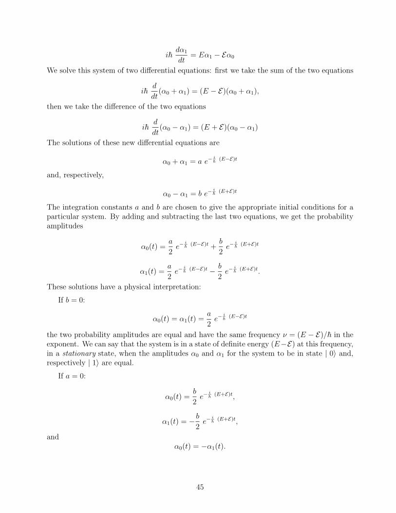
i�dα1

dt= Eα1 − Eα0

We solve this system of two differential equations: first we take the sum of the two equations

i�d

dt(α0 + α1) = (E − E)(α0 + α1),

then we take the difference of the two equations

i�d

dt(α0 − α1) = (E + E)(α0 − α1)

The solutions of these new differential equations are

α0 + α1 = a e−i�

(E−E)t

and, respectively,

α0 − α1 = b e−i�

(E+E)t

The integration constants a and b are chosen to give the appropriate initial conditions for aparticular system. By adding and subtracting the last two equations, we get the probabilityamplitudes

α0(t) =a

2e−

i�

(E−E)t +b

2e−

i�

(E+E)t

α1(t) =a

2e−

i�

(E−E)t − b

2e−

i�

(E+E)t.

These solutions have a physical interpretation:

If b = 0:

α0(t) = α1(t) =a

2e−

i�

(E−E)t

the two probability amplitudes are equal and have the same frequency ν = (E − E)/� in theexponent. We can say that the system is in a state of definite energy (E−E) at this frequency,in a stationary state, when the amplitudes α0 and α1 for the system to be in state | 0〉 and,respectively | 1〉 are equal.

If a = 0:

α0(t) =b

2e−

i�

(E+E)t,

α1(t) = − b

2e−

i�

(E+E)t,

andα0(t) = −α1(t).

45

This is another possible stationary state. This time the two amplitudes have the frequency(E+E)/�. We say that the system is in a state of definite energy (E+E) if the two amplitudesare equal, but of opposite sign, i.e., α0 = −α1.

Now, let us assume that at t = 0 the system is in state | 0〉. Then:

α0(0) =a + b

2= 1

α1(0) =a − b

2= 0

with the resulta = b = 1

The amplitudes become

α0(t) = e−i�

Et

(e

i�

Et + e−i�

Et

2

)

α1(t) = e−i�

Et

(e

i�

Et − e−i�

Et

2

)

and we can rewrite them as

α0(t) = e−i�

Et cosEt

�

α1(t) = e−i�

Et sinEt

�.

The probability that the system is found in state | 0〉 at time t is

| α0(t) |2= cos2 Et

�.

The probability that the system is in state | 1〉 at time t is

| α1(t) |2= sin2 Et

�.

At the initial moment t = 0 the probability that the system is in state | 1〉 is zero, increasesto one and continues to oscillate between zero and one in time. The probability that thesystem is in state | 0〉 is one at the initial moment, t = 0, decreases to zero and then oscillatesbetween one and zero in time. We say that the magnitude of the two probability amplitudesvaries harmonically 3 with time. The probability to find the system in one of the two statesvaries back and forth between the magnitudes of the two individual probabilities.

3A harmonic variation is expressed in complex exponential form as Aei(ωt+ε), where ω = 2πν is the angularvelocity.

46

1.7 Measurement Postulate

The numerical outcome of a measurement of observable A of a quantum system in state| ϕ〉 ∈ Hn is an eigenvalue λi of the operator A used to measure observable A; immediately

after the measurement, the quantum state of the system is an eigenvector | ai〉 of Acorresponding to the eigenvalue λi.

This postulate is sometimes called the postulate of collapse because as we shall see later ameasurement projects, or collapses, the state of the quantum system being measured.

Another formulation of this postulate is that mutually exclusive measurement outcomescorrespond to orthogonal projection operators (projectors) {P0,P1, . . .}. From the definitionof a complete set of orthogonal projectors it follows that the number of projectors in a com-plete orthogonal set must be less than, or equal to the dimension of the Hilbert space. Themeasurements postulate can be reformulated in terms of completeness of a set of projectors:a complete set of orthogonal projectors specifies an exhaustive measurement.

The resulting state after applying the transformation given by Pi to a quantum system instate | ϕ〉 is

| ψ〉 = Pi | ϕ〉.The probability of obtaining a measurement outcome λi is the norm of the resulting state

p(λi) =| | ψ〉 |2=| Pi | ϕ〉 |2= (Pi | ϕ〉)† Pi | ϕ〉 = 〈ϕ | P†iPi | ϕ〉 = 〈ϕ | (Pi)

2 | ϕ〉.

But (Pi)2 = Pi thus,

p(λi) = 〈ϕ | Pi | ϕ〉.The completeness of the set of projectors implies that the total probability for all possiblemeasurement outcomes is

∑i p(λi) = 1. It follows that∑

i

〈ϕ | Pi | ϕ〉 = 1.

After the measurement, the state | ψ〉 becomes a normalized pure quantum state defined as

| ψ′〉 =| ψ〉√

〈ϕ | Pi | ϕ〉=

Pi | ϕ〉√〈ϕ | Pi | ϕ〉

.

Example. Consider a two-dimensional Hilbert space, H2 where we have chosen the orthogonalbasis vectors | x〉 and | y〉. We define two possible state vectors of a system in this space

| ϕA〉 = αx | x〉 + αy | y〉 and | ϕB〉 = βx | x〉 + βy | y〉The initial state of the system could be | ψA〉 with probability p or | ψB〉 with probability1 − p; we say that the system is in a mixed ensemble of quantum states.

47

Quantum system in state

Hermitian operator A with n

eigenvectors: |ei>

eigenvalues:

Observable A

>∈φ| niλ

n projectors

{P1, P2 ...Pi ...Pn }

Pi = |ei><ei |PiA ∑

=

=n

i

iλ

1

P1

New state: P1

Outcome of the measurement:

Probability of the outcome:

>∈φ| n

1λ

Pi

New state: Pi

Outcome of the measurement:

Probability of the outcome:iλ

∑=

n

i 1

Pi =1

>∈φ| n

Pi

2|| >φ

New state: Pn

Outcome of the measurement:

Probability of the outcome:

>∈φ| n

2|| >φ

2|| >φ|P1

Pn

Pn

nλ

Figure 6: The measurement of observable A of a quantum system in state | ϕ〉 ∈ Hn. Theoperator A corresponding to observable A is Hermitian and has n eigenvalues, λi ∈ R, 1 ≤i ≤ n. The corresponding eigenvectors | ei〉, 1 ≤ i ≤ n form an eigenbasis. The set of nprojectors Pi is complete if

∑ni=1 Pi = I; the state of the system after the transformation due

to Pi is | ψi〉 = Pi | ϕ〉, the outcome of the measurement is λi and the Prob(λi) =| Pi | ϕ〉 |2.

We perform a large number, N , of measurements corresponding to the projectors

Px =| x〉〈x | and Py =| y〉〈y | .

We wish to predict nx, the number of times out of the total number N of measurements,when we expect to obtain the measurement outcome corresponding to basis vector | x〉. Weuse the conditional probabilities Prob(x| | ϕA〉) and Prob(x| | ϕB〉) to express nx as

nx = N [Prob(| ϕA〉) · Prob(x| | ϕA〉) + Prob(| ϕB〉) · Prob(x| | ϕB〉)]

= N [p 〈ϕA | Px | ϕA〉 + (1 − p)〈ϕB | Px | ϕB〉]

= N [p | αx |2 +(1 − p) | βx |2]

48

The ratio nx/N is bounded from below by the smaller of | αx |2 and | βx |2 as 0 ≤ p ≤ 1.Let us assume that the initial state of the system is a coherent superposition of the states

| ϕA〉 and | ϕB〉 corresponding to the pure state | ϕ(γA, γB)〉, with

| ϕ(γA, γB)〉 = γA | ϕA〉 + γB | ϕB〉

= (γAαx + γBβx) | x〉 + (γAαy + γBβy) | y〉,

were γA and γB are chosen such that the state | ϕ(γA, γB)〉 is normalized, | γA |2 + | γB |2= 1.In this case, the probability of a measurement outcome corresponding to basis vector | x〉

is nx/N :nx

N= 〈ϕ(γA, γB) | Px | ϕ(γA, γB)〉

= | γAαx + γBβx |2We notice that in certain cases it is possible to choose γA and γB such that γAαx = −γBβx �= 0and then, nx = 0 though | αx |2, | βx |2 > 0. This phenomenon is known as destructiveinterference.

There is an important distinction between coherent superpositions (of the type that pro-duce a single pure state) and the incoherent admixtures (of the type that produce a mixedensemble of quantum states).

Now we summarize several important properties of the quantum observables and quantumoperators related to the concepts discussed in this section:

1. An observable in Quantum Mechanics is a Hermitian operator with a complete set ofeigenvectors. This set of eigenvectors can be chosen to be mutually orthogonal; theyform a basis.

2. The eigenvalues of a Hermitian operator are real numbers.

3. Eigenvectors of a Hermitian operator corresponding to different eigenvalues are mutuallyorthogonal.

4. If two Hermitian operators commute, they have a common basis of orthonormal eigen-vectors (an eigenbasis). If they do not commute, then no common eigenbasis exists.

5. A complete set of commuting observables is the minimal set of Hermitian operators witha unique common eigenbasis.

6. The eigenvalues of a unitary operator are complex numbers of modulus 1.

7. Eigenvectors of a unitary operator corresponding to different eigenvalues are mutuallyorthogonal.

8. In general, an operator must be normal for the property of orthogonality of eigenvectorsto hold.

9. If A is a Hermitian operator, and A is an observable of a system, then the measurementof observable A of the system in state | ϕ〉 leaves the system in a state which is aneigenvector | a〉 of A and the probability of this outcome is | 〈a | ϕ〉 |2.

49

1.8 Linear Algebra and Systems Dynamics

Linear algebra allows us to describe the evolution in time of classical, as well as quantumsystems. Consider first a discrete-time, finite-dimensional, non-deterministic classical system;the state transitions occur at distinct time instances t1, t2, . . . , tk, . . .; the state space is ofdimension n. The state of the system at time tk is a stochastic vector, σ = (pk

1, pk2, . . . , p

kn)

with∑

i pki = 1 and pk

i the probability of the system being in state i, 1 ≤ i ≤ n, at time tk.The dynamics of the system is captured by a directed graph G with vertices corresponding tothe states; the arcs correspond to transitions and are labelled with the transition probabilities.This graph is characterized by the adjacency matrix A = [aij] with aij the probability of thetransition from state i to state j. The adjacency matrix A is a row stochastic matrix, the sumof all elements in a row is equal to 1.

3/14/1

1/2

1/4

1/4 7/12 1/21/6

1/6

p1=1/2

p2=1/4

p3=1/4

Figure 7: Systems dynamics. The directed graph G with adjacency matrix A.

For example, in the graph in Figure 7 the state of the system is given by the vectorσT (tk) = (1/2 1/4 1/4) and the adjacency matrix is

A =

⎛⎝ 1/4 1/2 1/4

1/6 1/3 1/27/12 1/6 1/4

⎞⎠

If the system is in state σtk at time tk, then the state at time tk+1 will be σtk+1= Aσtk :

σtk+1=

⎛⎝ 1/4 1/2 1/4

1/6 1/3 1/27/12 1/6 1/4

⎞⎠⎛⎝ 1/2

1/41/4

⎞⎠ =

⎛⎝ 5/16

7/2419/48

⎞⎠ .

The next state of a classical Markovian discrete-time stochastic system depends only on thecurrent state. The system could reach a state σi from two distinct initial states, σa and σb;the memoryless property does not allow to distinguish which path was taken to reach σi andmakes it impossible to return to the initial state, the system is non-reversible. Only if A isa permutation matrix, a matrix with one non-zero element in each row and each column,the discrete-time system is reversible. The description of a classical stochastic system with acontinuous-time and a possibly infinite state space is considerably more complex and will notbe discussed.

50

We have been concerned with the dynamics of classical systems where probabilities arereal numbers 0 ≤ pi, pj ≤ 1 and

∑i pi = 1; then probabilities can only increase when added,

pi + pj ≥ pi and pi + pj ≥ pj. What if the probabilities are functions of complex numbers,e.g., they are the square of the modulus of complex numbers, | qi |2=| αi + iβi |2, and wereplace the condition

∑i pi = 1 with

∑i | qi |2=

∑i(α

2i + β2

i ) = 1.With these rules in place we notice that | q1 + q2 |2 can be smaller than | q1 |2 or | q2 |2.

For example, if q1 = 3 + 5i and q2 = −4 − 4i, then | q1 |2= 9 + 25 = 34, | q2 |2= 16 + 16 = 32and | q1 + q2 |2=| (3 − 4) + i(5 − 4) |2= 1 + 1 = 2.

The arcs in the directed graphs are now labelled with complex numbers and we now requirethat the adjacency matrix be unitary, rather than row stochastic. If qij is the label of the arcfrom state i to state j then the adjacency matrix is

Q = Q[qij] and QQ† = I

Then:

| σt+1〉 = Q | σt〉 =⇒ 〈σt |= 〈σt+1 | Q.

Indeed, | σt+1〉 = Q | σt〉 implies that 〈σt+1 |= 〈σt | Q† and 〈σt+1 | Q = 〈σt | Q†Q = 〈σt |.A logical question we address next is why we choose the transition probabilities for a

discrete-time quantum system to be functions of complex numbers. The answer is that thenew probability rules allow us to capture the wave-like behavior of atomic and subatomicparticles while the real-valued probabilities describe classical, particle-like behavior.

The wave-particle duality and the new probability rule. One of the greatestdiscoveries leading to the formulation of wave equation of Schrodinger in 1926 was thewave-particle duality principle formulated by Louis de Broglie in 1923; this principle statesthat atomic and subatomic particles (matter) and photons (energy) exhibit both wave-likeand particle-like properties. The wavelength λ and the momentum p of any form of matterare related: λ = h/p with h Planck’s constant.

To grasp the physical significance of the probability rules we consider the double-slitexperiments discussed [149]. When the experiment is performed with bullets and when bothslits are open the number of bullets n(x) collected at a spot x between the two slits is thesum n(x) = nup(x) + nlow(x), with nup(x) the number of bullets when only the upper slit isopen and nlow(x) is the number of bullets when only the lower slit is open. If N bullets areshot and p(x) = n(x)/N is the probability of a bullet hitting spot x with both slits open,pup(x) = nup(x)/N and plow(x) = nlow(x)/N correspond to the two probabilities with onlyone slit open, then the usual probability rule applies: p(x) = pup(x) + plow(x).

When the double slit experiment is performed with waves, then in some spots the ampli-tude a(x) of the waves is reinforced a(x) > max(aup, alow), while in other spots it is diminished,a(y) < min(aup(y), alow(y)). This is due to the phenomenon of interference characteristic towave-like behavior.

In conclusion, state transformation in a Hilbert space corresponds to application of a uni-tary operator to the current state and the probability of a state is the modulus of a complexnumber. For example in H2 a system in state:

| ϕ〉 = α0 | 0〉 + α1 | 1〉

51

has the probability p0 =| α0 |2 to be in state | 0〉 and the probability p1 =| α1 |2 to be instate | 1〉 with | α0 |2 + | α1 |2= 1. This system will be the embodiment of a unit of quantuminformation called a qubit.

1.9 Symmetry and Dynamic Evolution

Symmetry plays an important role in classical as well as quantum physics. The mathematicalconcept which describes the symmetry of a physical system or of a physical object is theconcept of a group. An abstract group is a set G equipped with a map g : G × G �→ G and(g)−1 : G �→ G and an element e ∈ G so that the familiar axioms discussed in Section 4.4hold. A subgroup G′ of the group G is a subset such that g1, g2 ∈ G′ implies g1 · g−1

2 ∈ G′.The set of symmetries of a physical system form a group; one can compose two symmetries,

consider the inverse of each symmetry, and there always exists the “identity” as an obvioussymmetry. Most of these groups belong to a remarkable class of groups, the Lie groups. Anabstract Lie group satisfies the axioms of a group and, in addition, is a “smooth manifold”4

such that both the composition and the inverse are given by differentiable functions. Themost familiar group is GL(n, F ), the group of symmetries of an n-dimensional vector spaceover the field F of real or complex numbers.

Almost all Lie groups can be described as subgroups of GL(n, R) or GL(n, C). For exam-ple, SL(n, R), the group of symmetries of R

n which preserves the n-dimensional volume, isthe subgroup of GL(n, R) consisting of matrices with a determinant equal to 1. As anotherexample, O(n, R), the group of symmetries of the vector space R

n which preserves the anglesand the distances, is a subgroup of matrices A with real elements and AAT = I. Also, U(n),the group of symmetries of the Hilbert space C

n is the subgroup of matrices A in GL(n, C)with AA† = I.

Lie algebra is a mathematical object which is mathematically, rather than conceptually,simpler than a Lie group. To each Lie group one can associate a Lie algebra; if the Lie group isa group of symmetries, then the Lie algebra is usually called infinitesimal symmetries. Eachfinite-dimensional Lie algebra determines an unique (connected and simply connected) Liegroup.

A Lie algebra is a vector space V over a field F together with a binary operation [, ]called a Lie bracket with the following properties:

1. Bilinearity:

[αu + βv, w] = α[u,w] + β[v, w], [w, αu + βv] = α[w, u] + β[w, v], ∀α, β ∈ F, ∀u, v, w ∈ V.

2. The Lie bracket [u, u]:

[u, u] = 0, ∀u ∈ V.

3. Jacobi identity:

[u, [v, w]] + [v, [w, u]] + [w, [u, v]] = 0, ∀u, v, w ∈ V.

4A smooth manifold is a geometrical object which is locally the same as the Euclidian space Rn [269]

52

The operation defined by the Lie bracket is not in general associative [[x, y], z] need not equal[x, [y, z]].

The Lie algebra of GL(n, F ) is denoted by gl(n, F ) and is the vector space of all n × nmatrices with elements from the field F and bracket [A,B] = A · B − B · A. The Lie algebraof SL(n, R and O(n, R), are subspaces of n× n matrices A with real elements and tr(A) = 0,respectively A + AT = 0 (skew symmetric matrices). The Lie algebra of U(n), denoted byu(n) consists of n×n matrices with complex elements which satisfy A + A† = 0, equivalentlywith matrices A such that (iA) is a Hermitian matrix.

An element in the Lie algebra defines a smooth one-parameter family of elements in theLie group parameterized by t ∈ R which for t = 0 is exactly e. Any smooth one-parameterfamily of elements in the group which, for t = 0 is e, an element in the Lie algebra of thegroup. If an n × n-matrix A is an element of gl(n, F ) then the one-parameter family is

etA = I +tA

1!+

(tA)2

2!+ . . . .

This series is convergent for any t to an invertible matrix. If A(t) is an one-parameter familyof elements in gl(n, F ) the

dA(t)

dt|t=0

is a matrix, not necessary invertible, hence an element in gl(n, F ).The non-commutativity of the Lie group is reflected in the bracket operation; more pre-

cisely if

A =dA(t)

dt|t=0 and B =

dB(t)

dt|t=0

then

limt→0

A(t)B(t)A(t)−1B(t)−1 − I

t2= [A,B].

In particular

[A,B] = limt→0

etA · etB · e−tA · e−tB − I

t2

The equality can be verified by applying l’Hospital rule from calculus.Usually the elements of a Lie algebra of a Lie group of symmetries, i.e. infinitesimal

symmetries, define conservation laws (first observed by Nother [14]).If an observable A (a self-adjoint operator) is invariant by the dynamics of a quantum

system defined by the Hamiltonian H (i.e., all eigenstates and eigenvalues are preserved by

the dynamics) which means Ae−i�

tH = e−i�

tHA (Section 1.6); one obtains (by derivation att = 0) [H,A] = 0. This holds even in the more general case when the dynamics is defined bythe time-dependent Hamiltonian H(t); precisely, [H(t),A] = 0.

53

1.10 Uncertainty Principle; Minimum Uncertainty States

In classical Physics the nondeterminism is due to uncontrolled causes that are recognizedto exist and that, if better known, would make the predictions better. The quantum statepostulate reveals the critical role of the non-determinism in quantum theory; the uncertaintyprinciple shows that it has broader implications on our ability to observe the properties of aquantum system and makes us wonder if its nature is fundamentally different from the roleit plays in classical Physics.

In quantum physics nondeterminism means that a precise knowledge at the quantum levelis impossible. The uncertainty principle introduced by Werner Heisenberg in 1927, is at theheart of the special nature of the nondeterminism of Quantum Mechanics. Uncertainty is anintrinsic property of quantum systems. The accuracy of measured values of physical proper-ties, such as position and momentum along the axis used to measure the position, is limited;the precise knowledge of both the position and the momentum is forbidden in a quantumsystem. This limitation cannot be avoided, as shown by many experiments performed overthe years. Einstein, who doubted that “God is playing dice,” questioned the truth of such anindeterminacy.

The uncertainty principle: consider canonically conjugated observables, x the position ofa particle and px the momentum of the same particle at position x; x and px are three-dimensional vectors and we consider their projections along the same direction d. Then Δx,the uncertainty in determining the projection of the position, and Δpx, the uncertainty indetermining the projection of the momentum at position x along the same direction, areconstrained by the inequality:

Δx Δpx ≥ �

2

where � = h/2π is the reduced Planck’s constant.Let us assume that we are interested in two observables A and B of a quantum particle,

associated with the Hermitian operators A and B, respectively. We prepare two disjoint setsS1 and S2 each set consisting of a large number of quantum systems in the identical state | ϕ〉.For the systems in S1 we measure first the observable A and then the observable B on allparticles. We obtain the “same” value for the observable A, while we notice a large standarddeviation of the observable B. For the systems in S2 we measure first the observable B andthen the observable A. Now we obtain the same value for the observable B, while we noticea large standard deviation of the observable A.

Call ΔA and ΔB the standard deviation of the measurements of observables A and B,respectively. The uncertainty principle can be expressed as

ΔA ΔB ≥ 1

2| 〈ϕ | [A,B] | ϕ〉 | .

with [A,B] the commutator of the two operators, A and B. If A and B are non-commutativequantum observables then [A,B] > 0; it follows that ΔAΔB > 0 thus, there is a minimumlevel of uncertainty that cannot possibly be removed.

On the other hand, when two operators commute, then they can be diagonalized simultane-ously and we can measure the eigenvalues of one of them without disturbing the eigenvectors

54

of the other. This property is important for a class of quantum error correcting codes, thestabilizer codes, discussed in Section 5.12.

The quantum mechanical uncertainty relation Δx Δpx ≥ �

2has a classical counterpart

based on the wave phenomena; an acoustic signal with intensity s(t) cannot have precisetiming and precise pitch, the two must satisfy the inequality:

Δt Δω ≥ 1

2where:

(Δt)2 ≡∫

t2s(t)dt −(∫

ts(t)dt

)2

and (Δω)2 ≡∫

ω2S(w)dω −(∫

ωS(ω)dω

)2

.

In this expression S(ω) = F (s(t)) is the Fourier transform of the function s(t) and ω =(2π)/f , with f = 1/T the frequency and T the period of the signal.

Peres observes [325] that in the case of acoustic signals we can have approximate valuesfor the time and the frequency; musical scores indicate both time and frequency and allowmusicians to produce sounds that capture the information generated by the composer. Itseems quite reasonable to consider also approximate values for the observables of a quantumsystem. For example, we can consider a Gaussian distribution of the position and wavelength,λ = h/p, of a wave packet with mean: x and variance σ, and, respectively, p. Then the wavefunction:

φ(x) = (πσ2)−1/4 exp

[x − x

2σ2

]+

1

�ipx

is a minimum uncertainty wave packet with:

Δx =1√2σ, Δp =

�√2σ and Δx Δp =

�

2σ2.

Minimum uncertainty wave functions can be extended to non-commuting operators otherthan position and momentum [325]. Coherent superposition states, introduced in Section 1.7and discussed in more depth in Section 3.16, are minimum uncertainty states.

1.11 Pure and Mixed Quantum States

So far, our discussion was focused on a class of states of a quantum system, described byDirac’s ket and bra vectors, or, by a wave function in a finite-dimensional Hilbert space.These states are called pure quantum states; a pure state can be expressed as a superpositionof the basis vectors of an orthonormal basis B = {| b1〉, | b2〉, . . . , | bn〉} ∈ Hn as

| ψ〉 =n∑

i=1

αi | bi〉 withn∑

i=1

| αi |2= 1.

A pure state that is a linear combination of two or more component states is sometimes calleda coherent superposition. According to the postulates of Quantum Mechanics, discussed in

55

Section 1.4, the evolution of a closed quantum system can be completely described as a unitarytransformation of pure states in a Hilbert space.

For a qubit in a coherent superposition state there is always a basis in which any mea-surement of the qubit will produces the same result. For example, the state

| ψ〉 =1√2(| 0〉+ | 1〉)

represents a qubit which has a 50% probability to produce either a “0” or a “1” as a resultof a measurement. If we rotate the basis by 45◦ by applying a Hadamard transformation, H,the state of the qubit becomes

H | ψ〉 =1√2

(1 11 −1

)1√2

(11

)=

(10

)and all measurements of the resulting state | 0〉, produce the same result, “0.”

We introduce a new characterization of the state of a quantum system by means of thedensity operator. We can associate every vector | ψ〉 ∈ Hn with a matrix A ∈ C

n×n; indeed,C

n×n, the set of n×n matrices with complex elements, is an inner-product vector space thus,there is an isomorphism from a Hilbert space to C

n×n. The density matrix of a pure state is

| ψ〉 =n∑

i=1

αi | bi〉 withn∑

i=1

| αi |2= 1.

The density matrix of a pure state | ψ〉 is given by the outer product

ρ =| ψ〉〈ψ |=

⎛⎜⎜⎜⎝

α1α∗1 α1α

∗2 . . . α1α

∗n

α2α∗1 α2α

∗2 . . . α2α

∗n

......

...αnα∗

1 αnα∗2 . . . αnα∗

n

⎞⎟⎟⎟⎠ .

The density matrix of a pure state is a Hermitian operator

ρ† = (| ψ〉〈ψ |)† =| ψ〉〈ψ |= ρ.

The trace of the density matrix of a pure state is equal to one

tr(ρ) =n∑

i=1

αiα∗i =

n∑i=q

| αi |2= 1.

A mixed state is a statistical ensemble {(| ψ1〉, p1), (| ψ2〉, p2), . . . , (| ψn〉, pn), } with pi aprobability in the classical sense,

∑ni=1 pi = 1, rather than a probability amplitude. The

density matrix of a mixed state∑n

i=1 pi | ψi〉 ∈ Hn is defined as

ρ =n∑

i=1

pi | ψi〉〈ψi |

56

where more than one factor pi is greater than zero. The density matrix of a mixed state isa Hermitian operator and its trace is one. Different mixtures of pure states could have thesame density matrix; for example, the mix of the pair of states

| +〉 =1√2(| 0〉+ | 1〉) and | −〉 =

1√2(| 0〉− | 1〉)

with probability p = 1/2 and the mix of pair of states | 0〉 and | 1〉 with probability p = 1/2have the same density matrix. See also Section 2.3 where we show that the density matrixallows us to distinguish pure states from mixed (impure) states: tr (ρ2) = 1 for a pure stateand tr (ρ2) < 1 for a mixed state. Pure states are represented as points on the surface ofthe Bloch sphere while mixed states are points inside the Bloch ball. An incoherent mixtureremains a mixture whatever basis we choose to describe it.

The density matrix plays an important role in quantum information theory, it providesan answer to the question “how much information can we acquire about a quantum state?”Pure states are characterized by maximal knowledge or minimal ignorance; in principle thereis nothing more to be learned about a quantum system in a pure state [44]. Whenever wecan only attribute probabilities to possible states, or when we are allowed to observe only asubsystem of a composed system, we cannot acquire maximum information about the entirequantum system and we say that the system is in a mixed state. The density operator ρ allowsus to distinguish pure from mixed quantum states; ρ is a Hermitian operator and tr(ρ) = 1.

1.12 Entanglement; Bell States

We discussed a number of intriguing properties of quantum states and we add to this list theentanglement, a phenomena without a classical counterpart. Quantum mechanical systemshave a unique property: a bipartite system, a system composed of two subsystems, can bein a pure state for which it is not possible to assign a definite state to each of its componentsubsystems. This strong correlation of quantum states is called entanglement; entangledstates are pure states of bipartite quantum systems.

Erwin Schrodinger discovered the phenomenon of entanglement5 and in 1935 he madea crucial observation: “total knowledge of a composite system does not necessarily includemaximal knowledge of all its parts, not even when these are fully separated from each otherand at the moment are not influencing each other at all.”

Charles Bennett and Peter Shor comment on the effect of entanglement for quantuminformation processing [44]: “classical information can be copied freely, but can only betransmitted forward in time to a receiver in the sender’s forward light cone. Entanglement, bycontrast cannot be copied, but can connect any two points in space-time. Conventional data-processing operations destroy entanglement, but quantum operations can create it, preserveit and use it for various purposes, notably speeding up certain computations and assisting inthe transmission of classical data or intact quantum states (teleportation) from a sender to areceiver.”

5Entanglement is the English translation of the German noun Verschrankung, the name used by Schrodingerto describe this phenomena.

57

According to the postulates of Quantum Mechanics the joint state of two or more quan-tum systems is a vector in a Hilbert defined as the tensor product of the Hilbert spacesHn1 ,Hn2 . . .Hnk

used to represent the individual states of the component systems

Hn1×n2···×nk= Hn1 ⊗Hn2 . . . ⊗Hnk

.

For example, the state of a quantum system consisting of two qubits is a vector in H22 =H2 ⊗H2 with the orthonormal basis {| 00〉, | 01〉, | 10〉, | 11〉} expressed as

| ψ〉 = α00 | 00〉 + α01 | 01〉 + α10 | 10〉 + α11 | 11〉with | α00 |2 + | α01 |2 + | α10 |2 + | α11 |2= 1.

Sometimes the state of a two-qubit system can be factored as the tensor product of theindividual states of two qubits. For example, when α00 = α10 = 1/2 and α01 = α11 = −i/2the state | ψ〉 is the tensor product of the states of the two qubits, | ψ1〉 and | ψ2〉

| ψ〉 = 12[| 00〉 − i | 01〉+ | 10〉 − i | 11〉]

= 12[| 0〉 ⊗ (| 0〉 − i | 1〉)+ | 1〉 ⊗ (| 0〉 − i | 1〉)]

= 12(| 0〉+ | 1〉) ⊗ (| 0〉 − i | 1〉)

= | ψ1〉⊗ | ψ2〉.The individual states of the two qubits are well-defined

| ψ1〉 =1√2(| 0〉+ | 1〉) and | ψ2〉 =

1√2(| 0〉 − i | 1〉).

This factorization is not always feasible. For example, consider a special state of a two-qubitsystem when

α00 = α11 = 1/√

2 and α01 = α10 = 0.

The resulting state | β00〉 is called a Bell state and the pair of qubits is called an EPR pair

| β00〉 =| 00〉+ | 11〉√

2.

There are three other Bell states

| β01〉 =| 01〉+ | 10〉√

2, | β10〉 =

| 00〉− | 11〉√2

, and | β11〉 =| 01〉− | 10〉√

2.

These states form an orthonormal basis and can be distinguished from one another. Bellstates are entangled states; the four states are called maximally entangled states and | β11〉 isan anti-correlated state.

Entangled states are never in an ideal form; the source producing the entangled state isaffected by noise and the communication channel used to transfer entangled states or the

58

quantum circuits used to manipulate the states can add noise. Thus we have to purify,or distill partial entanglement. Assume we have N pairs of qubits, each pair in the sameentangled but mixed state with density matrix ρ; the ensemble of pairs is in the state givenby the N -fold tensor product ρ⊗N . Several protocols exist to transform the set of the N pairsof partially entangled pairs to M < N pairs of maximally entangled particles using only localoperations and classical communication primitives [39, 40, 119].

Entangled states are affected by decoherence; the environment conspires to disentanglethe quantum systems we have prepared in an entangled state. and we have to protect theinformation embodied by entangled quantum states. The fragility of quantum informationrequires that we encode quantum states and then manipulate them in an encoded form.

After this introduction of basic concepts of quantum physics we review several aspectsof quantum information processing. We start with a discussion of quantum information andthen introduces quantum computational devices and quantum algorithms.

1.13 Quantum Information

The unit of classical information is a bit with two possible values, B = {0, 1}; n bits forma register R = {0, 1}n. The state of a system can characterized by the m = 2n possibleconfigurations of the bits in register R. The vector (p1p2 . . . pm) with

∑i pi = 1 and the

(m×m) adjacency matrix P describe the evolution of the system. A reversible transformationof the system state is described by a permutation matrix P , a matrix with only one non-zeroelement in each row and column; the new state is P (p1p2 . . . pm)T .

When the physical support of information is a quantum system we talk about quantuminformation. The unit of quantum information is a qubit abstracted as C2 = {| 0〉, | 1〉};a register of n qubits is (C2)⊗n and the reversible transformation of the state of a quantumsystem are described by a unitary transformation. The density matrix ρ allows the descriptionof pure as well as mixed states with the probability of the individual components of the mixdescribed by the vector q1q2 . . . qn and

∑i qi = 1; ρ is a diagonal matrix with qi as its elements;

a reversible transformation transforms the density matrix ρ in ρ′ with ρ′ = PρP †.As expected, properties of quantum quantum systems such as entanglement and superpo-

sition, the inability to clone the state of a quantum system, the fact that a measurement is anirreversible process, and the instability of quantum states due to interactions with the envi-ronment have a profound effect on the ways we process quantum information. The questionwe pose now is if this new embodiment of information leads to special attributes that can beexploited in the process of manipulating information.

Superposition. The wave-particle duality characterizes the behavior of quantum sys-tems; interference occurs as a manifestation of the wave behavior and is a consequence ofthe superposition of quantum states. Due to superposition we can compute the 2n values ofa function f(x) with x a binary n-tuple in one time step using a single copy of a quantumcircuit implementing the transformation f(x) of its input x. For example, consider a lengthycomputation of a function f(x) where the argument x is one bit and the result is also onebit, f(0) or f(1). We are not interested in the actual value of the function, but only if thefunction is constant, f(0) = f(1), or balanced, f(0) �= f(1). A sequential classical computerevaluates first f(0), then f(1), and finally compares the two to provide the answer; a parallel

59

classical computer evaluates f(0) and f(1) concurrently, but needs two processors for thistask. A quantum computer with the input a superposition of | 0〉 and | 1〉 allows us to extractglobal information about the function f and thus to solve Deutsch’s problem in a single timestep (the time needed to evaluate the function for one value of the argument), and with asingle copy of the hardware, see Section 1.19.

We are now in a better position to understand Feynman’s argument that the exact simu-lation of a quantum system is only possible with a quantum computer; assume that a stateof the quantum system used for the exact quantum simulation can be expressed using n bitswith n a large number, e.g., n = 103. Such a state is described by 2n = 21000 ≈ 10333 complexnumbers. No classical computer is able to store and process this colossal amount of data;on the other hand the exact simulation of the system can be carried out with a quantumcomputer, provided that we expect the answer either to be that the resulting state is identicalwith a reference state or not, or to provide a measure of their distance.

We are capable of simulating the behavior of quantum circuits using classical computers,a problem critical for the study of quantum fault-tolerance [1, 108, 439]. The simulation ofquantum circuits is possible when the behavior of the quantum system is confined to a smallregion of the vast Hilbert space.

Entanglement. The entanglement of quantum systems has a profound impact on quan-tum information processing. Consider a composite quantum system consisting of two subsys-tems A and B with n and m qubits, respectively. The question we pose is if it is possibleto reconstruct the state of the joint systems from measurements performed separately on oneof the subsystems alone. The answer to this question was given by John Bell [25, 26] whoestablished that the information about the quantum state of a composite system is containedin non-local correlations between the two subsystems; these non-local correlations cannot berevealed by any measurement performed on one of the subsystems alone.

We should point out that non-local correlations that cannot be revealed by measurementsperformed on only one of the component systems are not restricted to quantum phenomena.Think for example of two correlated random variables X and Y related to the behavior oftwo systems A and B, respectively; there are no local measurements which allows either Aor B to determine the joint probability density function, pXY (x, y). In addition to non-localcorrelations a critical property of the quantum entanglement is that a measurement of one ofthe two subsystems forces the other one to change its state, as we shall see when we discussthe EPR experiment in Section 2.16.

Entanglement has important implications for quantum error correction, a critical aspect ofquantum information processing. Entanglement allows us to detect quantum errors withoutaltering the state of the qubits in a quantum register, and then to correct the errors. First,we entangle the qubits in the register with ancilla qubits prepared in a well-defined state; asa result of the entanglement the ancilla qubits contain information about the qubits in error.Then we perform a non-demolition measurement of the ancilla qubits to determine the errorsyndrome. The error syndrome tells us if an error has occurred and if so which qubits wereaffected and what type of error was present. An undesirable consequence of entanglement isthe occurrence of spatial and time-correlated quantum errors. Once a qubit is affected by anerror, the error can propagate to other qubits correlated to the one in error; a time-correlatederror re-occurs at a later time, on the same qubit, after we have corrected its initial occurrence.

60

Preparation Measurement

PreparationMeasurement

Classical

Information

Quantum

Information

Figure 8: Classical and quantum information and conversion from one to another. Classicalinformation is represented by thin arrows and quantum information as thick arrows. (a) Clas-sical information can be regarded as a particular form of quantum information. (b) Classicalinformation can be recovered from the quantum information when the preparation phase isfollowed by a measurement. The conversion path is: classical �→ quantum �→ classical. (c)Quantum information cannot be recovered when the preparation follows the measurement;the measurement is an irreversible process and alters the state of quantum systems. Theconversion path in this case is quantum �→ classical �→ quantum.

Measurements, preparation, and extraction of classical information from quan-tum information. Classical information is independent of the medium used to transport it.Yet, classical information is often carried by the same types of particles as quantum informa-tion, e.g., electrons, or photons; why should we expect quantum information to be differentfrom classical information?

To answer this question we should establish if it is possible to freely convert one typeof information to another and then recover the original information [231]. We can convertclassical to quantum information and then convert back the quantum information to theoriginal classical information. Formally, this process consists of two stages: preparation, whenthe quantum information is generated from the classical one and measurements, when classicalinformation is obtained from the quantum information, Figure 8(a).

The remaining question is if we can convert quantum to classical information and thenconvert the classical information to quantum information indistinguishable from the originalone; this means that we should first perform a measurement to extract classical informationand then use it to prepare quantum information, Figure 8(b). The only possibility to comparequantum mechanical systems is in terms of statistical experiments and this is not possible,since a measurement is an irreversible process, it alters the state of a quantum system; Chapter2, devoted to quantum measurements, covers the arguments supporting this statement.

We conclude that indeed, quantum information is qualitatively different from the classicalone. Even though classical and quantum information can be carried out by the same typesof particles, the physical processes are different; in the former case the physical processesare subject to classical Physics and in the later to quantum Physics. As we shall see inChapter 2 some states of a quantum system, the pure states, have a classical counterpart and ameasurement allows us to distinguish orthogonal pure states. Therefore, classical informationcan be regarded as a particular form of quantum information, Figure 8 (c).

61

Manipulation of quantum states. Now we turn our attention to the the question if thestates of a quantum system are stable for sufficiently long periods of time to allow the transfor-mations prescribed by a quantum algorithm to progress without hinderance. Unfortunately,only rarely the state of a quantum system can be considered as being stable, more often theyare unstable. For example, the famous state of Schrodinger’s cat is a “superposition” of beingat the same time “dead” and ”alive” formally described as | cat〉 = 1√

2(| dead〉+ | alive〉).

This state is possible in Quantum Mechanics, but never observed in practice; all the catswe have ever seen, or will ever see were and will be either dead or alive. The instability ofquantum states is due to the interactions of the system with the environment; the correlationbetween a quantum system and the environment are very strong and lead to the phenomenonof decoherence which hinders quantum information processing.

The quantum information we wish to process is encoded as correlations among the compo-nents of the quantum system; the interactions of the environment with the quantum systemerode in time these useful correlations which are transformed to correlations between thequantum system and the environment. The decoherence is only one of the problems we haveto address when we think about building quantum computing and communication devices.

Another problem is the accumulation of errors, a problem we are familiar with from thestudy of classical analogue circuits; if each analog circuit performing the transformation Ti

introduces an error εi then, after N steps, instead of the desired transformation,∏N

i=1 Ti(I)

the transformation of the input I will be∏N

i=1 Ti(1 + εi)(I). Similarly, if each quantum gateintroduces a small error ε then, after 1/ε gates, the cumulated error will be significant enoughto affect the result.

In addition to the bit-flip errors we are familiar with from the study of fault-tolerance ofclassical systems, we have to deal with phase-flip errors and with combinations of bit- andphase-flip errors of a quantum system. This brief discussion motivates the attention paid toquantum error correction, one of the topics of this book.

Physical embodiment of quantum information. The quantum analog of a classicalbit is called a qubit; following our mantra that“information is physical” we link the abstractioncalled qubit with the physical reality and provide a glimpse at some of the properties ofquantum particles we have to manipulate in order to process quantum information.

Quantum particles have some properties with no classical counterpart. For example, thespin is an intrinsic angular momentum6 of a quantum particle, related to its intrinsic rotationabout an arbitrary direction. The spin of a quantum particle can be observed as the result ofthe interaction of the intrinsic angular momentum of the particle with an external magneticfield B. Classical Physics operates with the concept of angular momentum arising from arotation around a well-defined axis of a body.

There are two classes of quantum particles, those with spin multiple of one-half, calledfermions, and those with spin multiple of one, called bosons. The spin quantum number offermions can be s = +1/2, s = −1/2, or an odd multiple of s = ±1/2. Electrons, protons,and neutrons are fermions; the spin quantum number of bosons can be s = +1, s = −1,s = 0, or a multiple of ±1.

A quantum particle such as the electron is not a “body” in the classical sense and does not

6The intrinsic angular momentum of a quantum particle should be distinguished from its orbital angularmomentum.

62

have a defined axis of rotation. The electron is characterized by a charge with a non-stationaryspatial distribution. The variation in time of this charge distribution can be associated withan intrinsic rotation of the electron about directions randomly oriented in space.

One possible embodiment of a qubit is the spin of the electron, the quantum numbercharacterizing the intrinsic angular momentum of the electron; the electron spin has eitherthe value +1/2 or −1/2 along the measurement axis, regardless of what that axis is. Theintroduction of this two-valued quantum number for the electron led Pauli to postulate hisexclusion principle. According to Pauli’s exclusion principle, no more than two electrons canoccupy the same “orbit” and those two electrons must have anti-parallel spins.

Indistinguishability is a principle of Quantum Mechanics saying that all quantum particlesof the same type are alike; for example, we cannot distinguish an electron from another.Therefore the operation of swapping the position of two electrons in a systems with manyelectrons leaves the system’s state unchanged or, in other words, the operation is symmetricand it is represented by a unitary transformation acting on the wave function as discussedin Section 1.7. In three dimensions an exchange of two bosons is represented by an identityoperator; the wave function is invariant and we say that the particles obey Bose statistics.The exchange of two fermions in three dimensions changes the sign of the wave function; theparticles are said to obey Fermi statistics.

A photon7, a particle of light, is another important two-state quantum system used toembody a qubit; the quantum information can be encoded as the polarization of the photon.Photons differ from the 1/2-spin electrons in two ways: (1) they are massless and (2) theyhave spin one. A photon is characterized by its vector momentum (the vector momentumdetermines the frequency) and its polarization.

Light has a dual nature, wave-like and corpuscular-like; as an electromagnetic radiation,light consists of an electric and a magnetic field perpendicular to each other and, at the sametime, perpendicular to the direction the energy is transported by the electromagnetic wave;the electric field oscillates in a plane perpendicular to the direction of light and the way theelectric field vector travels in this plane defines the polarization of light.

When the end of the electric field vector oscillates along a straight line, we say that thelight is linearly polarized. When the end of the electric field vector moves along an ellipse,the light is elliptically polarized and when it moves around a circle, the light is circularlypolarized. If the light comes toward us and the end of the electric field vector moves aroundin a counterclockwise direction, we say that the light has right-hand polarization; if it movesin a clockwise direction, we say that the light has left-hand polarization.

The last embodiment of quantum information we discuss are the anyons, quantum parti-cles of interest for the topological quantum computing. Anyons are indistinguishable particlesdefined in two dimensions; they are different from either fermions or bosons. Consider a gasof electrons squeezed between two slabs of semiconductor materials such that, the movementof electrons is restricted to two dimensions only. At very low temperature and in a strongmagnetic field the two-dimensional electron gas has a strongly entangled ground (lowest en-ergy) state separated from all other states by an energy gap. This lowest-energy state carryan electric charge that is not an integer multiple of the electron charge and does not havethe quantum numbers associated with electrons [345]. The properties of the anyons manifestthemselves as the Fractional Quantum Hall Effect (FQHE) discovered by Daniel Tsui, Horst

7The name photon comes from the Greek word “photos” meaning light.

63

Stormer and Arthur Gossard [425]; the FQHE is discussed in Section 6.15.We have only mentioned three possible embodiments of quantum information, others are

discussed in detail in Chapter 6 that covers physical realizations of quantum computing andcommunication devices. The diversity of potential implementations of quantum informationprocessing devices is a source of optimism and, at the same time, anxiety. On one hand, itgives us great hope that at least some of the theoretical ideas will ultimately lead to feasiblequantum information processing devices; on the other hand, it gives as some feeling aboutthe vastness of the field and the depth of knowledge required to master a discipline involvingmultiple areas of Mathematics, Physics, and Computer Science.

Quantum information processing systems. The last subject of our survey of quan-tum information covers quantum information processing systems. A quantum computer is aphysical device capable of transforming quantum information as required by a quantum algo-rithm; a quantum communication system transmits either classical, or quantum informationfrom one place to another through a quantum channel.

The operation of a quantum computer takes advantage of fundamental principles of quan-tum Physics: superposition, quantum interference, quantum entanglement, and the high di-mensionality of the state space of a quantum system to solve some computationally “hard”problems efficiently. A quantum algorithm aims to increase the probability of obtaining thecorrect answer by arranging that all computational path leading to the right answer interfereconstructively, while the computational paths to wrong answers interfere destructively. Thisstrategy has been applied successfully for solving a subset of “hard” computational problemssuch as factoring large numbers and searching large unstructured databases; the quantumalgorithms of Shor [380] and Grover [183] are milestones in quantum computing.

To process information with a quantum system we first prepare the system in an initialquantum state, then transform this state through a set of operations prescribed by a quantumalgorithm, and, finally, measure the resulting state of the system. This sequence of stepsresembles the ones followed by a classical device up to the point when we examine the result.The qualitative difference between a classical system outputting the result of a transformationand the measurement of the final state of the quantum system is due to the randomness ofthe quantum measurement process. If the result of the quantum computation is one qubit instate | ψ〉 = α0 | 0〉 + α1 | 1〉 then a measurement of the qubit will produce the result 0 withprobability p0 =| α0 |2 or 1 with probability p1 =| α2 |2.

A quantum algorithm generates a probability distribution of the results while a random-izing algorithm for a classical computer uses randomness as part of its logic. There arequalitative differences between randomization algorithms and quantum algorithms. The for-mer are designed with the hope of achieving good performance in the ”average case” over allpossible random choices; the later exploit the entanglement and superposition of quantuminformation, the randomness is not part of their logic, but of the physical transformationsleading to the result.

In [265] Landauer observes that classical computers function based on the intuitive andcompletely abstract computability theory due to Church, Turing, Post, and Godel, while“the properties of quantum computers are not postulated in abstracto, but deduced from thelaws of physics” [118]. A quantum computer coupled with a quantum communication systemperforms functions related to quantum cryptography that are not feasible with a classicalsystem; however, a quantum computer can only perform computations that can be carried

64

out by a classical computer, albeit much more efficiently.A quantum communication channel transmits information using quantum effects when,

for example, the information is encoded as the spin of an electron or in the polarizationof a photon. Eavesdropping on a quantum communication channel can be detected witha very high probability because the effect of intrusion is an irreversible transformation, ameasurement of the quantum state.

We conclude that the special properties of quantum information have important conse-quences for computation and for communication and we should investigate the the physicalrealization of quantum information processing devices.

1.14 Physical Realization of Quantum Information Processing Sys-tems

A quantum computer is a physical device designed to transform quantum information em-bodied by the state of a quantum system. The physical processes required to transform thequantum state in a controlled manner are different for ion traps, solid-state, optical, NuclearMagnetic Resonance (NMR), or other possible physical implementations. Thus, we needfirst to define the basic requirements to build a quantum computer regardless of the physicalphenomena involved. DiVincenzo [131] provides a crisp and clear formulation of five plustwo (additional) requirements (discussed in depth in Section 6.1) for a quantum informationprocessing system:

1. A scalable physical system with well-characterized qubits.

2. The ability to initialize the state of the qubits.

3. Long relevant decoherence times, much longer than the gate operation times.

4. A “universal” set of quantum gates.

5. A qubit-specific measurement capability.

The two additional requirements are related to the ability to communicate:

1. The ability to inter-convert “stationary” (memory) and “flying” (communication)qubits.

2. The ability to faithfully transmit “flying” qubits between specified locations.

These requirements come naturally to mind, they have an immediate correspondent forclassical computers. Indeed, we cannot conceive a state of the art computer built with circuitswhose state cannot be controlled or be initialed to a desired state. It would be impractical tobuild a computer unless we have a finite set of building blocks and it seems obvious that weshould have access to the results of a computation.

A well-characterized qubit means that the relevant parameters of the physical process,including the Hamiltonian H(t) of the system and the coupling between a qubit and the

65

environment and between this qubit and other qubits, must be known. For an implementa-tion of a quantum computer we should only consider those quantum systems which satisfythis requirement. For example, the Super Selection Rules (SSR)8 prohibit entangled statesinvolving different particle numbers thus, a two-qubit system consisting of two quantum dotsand an electron in a superposition state as being on one or the other quantum dot would notsatisfy the first requirement [131].

The scalability requirement is not only related to the ability to carry out complex trans-formations, but also to the necessity, discussed later, of having reliable circuits; as we shallsee shortly, every “useful qubit” requires a large number of additional qubits, 10 or more, toensure fault-tolerance.

It is self-evident that we should prepare a qubit in a well-defined initial state in order tocarry out a quantum computation with predictable results. An n-qubit quantum computeroperates on a 2n-dimensional Hilbert space H2n with computational basis states | x1x2 . . . xn〉with xi = 0 or xi = 1. This requirement translates to the fact that any computational basisstate | x1x2 . . . xn〉 should be prepared in at most n steps. The practical questions are howto initialize a qubit in a state with maximal entropy and how fast the preparation of qubitscan be done. A possible solution is to have an independent system to prepare qubits in aninitial state either by forcing them to the ground state of the Hamiltonian, a process called“cooling,” or by performing a measurement which collapses the state of a qubit to a basisstate, e.g., | 0〉. Then, a “qubit conveyor belt” should provide access to the qubits in theinitial state whenever they are needed.

Decoherence in its simplest form means that a “pure state” | ϕ〉 = α0 | 0〉 + α1 | 1〉is transformed by interaction with the environment to a “mixed state” with density matrixρ =| α0 |2| 0〉〈0 | + | α1 |2| 1〉〈1 |. The pure state of a qubit is represented by a vectorconnecting the origin with a point on the surface of the Bloch sphere, while a mixed state ofa qubit is represented by a vector connecting the origin to a point inside the Bloch (solid)sphere; the von Neumann entropy of a mixed state is measured by the distance of such apoint to the surface of the Bloch sphere, as discussed in Section 2.3.

Since the early days of computing, reliability has been a major concern [80] therefore,it seems reasonable to ask ourselves if a reliable quantum computer could be built at all,knowing that quantum states are subject to decoherence. The initial thought was that aquantum computation could only be carried out successfully if its duration were shorterthan the decoherence time of the quantum computer. As we shall see in Section 5.25, thedecoherence time ranges from about 104 seconds for the nuclear spin, to 10−9 seconds for thequantum dot charge. Thus, it seemed very problematic that a quantum computer could bebuilt unless we have a mechanism to periodically deal with errors.

Probabilistic classical computer and communication systems can be error corrected andoperate effectively in the presence of noise without requiring an exponential precision whilethe operation of their analog counterparts is conditioned by a lack of noise and an exponentialprecision. The analog nature of quantum information and of quantum transformation raisedserious questions for the experimental realization of quantum information processing systems.

8An SSR is a restriction on the allowed local operations on a system, not on its allowed states, and it isassociated with a group of physical transformations [24]. Such restrictions could be imposed by the propertiesof the underlying theory, or arise due to physical restrictions. The operations it applies include unitarytransformations, Oρ = UρU†, and measurements, Orρ = MrρM†

r with∑MrM†

r = 1.

66

These questions were answered in [381], [403], [246], [40], [247], [248] showing that quantumcomputing and communication systems are more similar to probabilistic classical systemsthan to analog ones.

Now we know that quantum error correcting codes could be used to ensure fault-tolerantquantum computing; quantum error correction allows us to deal algorithmically with decoher-ence. A quantum error correcting code maps a “logical qubit” onto several “physical qubits”and then encodes these qubits using two classical error correcting codes to deal with bit-flipand phase-flip errors, as discussed in detail in Chapter 5. There is a significant price to payto achieve fault-tolerance through error correction, the number of qubits required to correcterrors is an order of magnitude larger than the number of “useful” qubits.

In 1996, Shor [383] showed how to perform reliable quantum computations when theprobability of a qubit or quantum gate error decays polylogarithmically with the size of thecomputation, a rather unrealistic assumption. The quantum threshold theorem states thatarbitrarily long computations can be carried out with high reliability provided that the errorrate is below an accuracy threshold according to Knill, Laflamme, and Zurek [247]. In 1999,Aharonow and Ben-Or [5] proved that reliable computing is possible when the error rate issmaller than a constant threshold, but the cost is polylogarithmic in time and space. Inpractice, error correction is successful for a quantum system whose decoherence time is fourto five orders of magnitude larger than the gate time, the time required for a quantum gateoperation.

In the next section we discuss in more detail the practical requirements regarding uni-versal quantum gates. Here we only note that the fact that any logic function could beimplemented using a small set of universal classical gates had a significant impact on currentsolid-state technology; it allowed us to reduce the size of classical circuits as predicted byMoore’s law which states that the number of transistors per chip that yields the minimumcost per transistor doubles every 18 months or so.

An important aspect of a discussion regarding universal quantum gates is that many-bodyquantum interactions are difficult to control and to analyze. Thus, it is necessary to have auniversal set of quantum gates which require at most two-body interactions, and this translatesto the ability to implement any unitary transformation using only one-qubit and two-qubitgates. Any unitary transformation can be approximated arbitrarily well by a quantum circuitconsisting of two-qubit CNOT gates, and one-qubit H, T, and S gates. First, we show thatany unitary transformation U ∈ H2n can be carried out by a set of unitary transformationsU1, U2, . . . Uk, . . . Um, with m ≤ 2n − 1, which act only on two or fewer computational basisstates. Then, we show that each unitary transformation Uk, 1 ≤ k ≤ m, can be expressedexactly as a product of transformations carried out by CNOT and one-qubit gates, and finally,we show that the transformation carried out by an one-qubit gate can be approximatedarbitrarily well by the transformations carried out by H, T, and S gates. As an examplewe show how to implement a Toffoli gate with the set of universal quantum gates describedabove.

Consider a quantum circuit that consists of m gates Gk, 1 ≤ k ≤ m, which carry out theunitary transformations Gk = eiHk(t)/�, 1 ≤ k ≤ m, with Hk(t) - the Hamiltonian describingthe evolution of the quantum system when implementing the k gate and � - Planck’s constant.The simplest modus operandi of the circuit is to consider discrete times t1, t2, . . . tk, . . . tm, tm+1

when each Hamiltonian is turned on and off. For example, Hk should be turned on at tk and

67

tuned off before tk+1 when Hk+1 is turned on.Recall that the control unit of a classical processor decides which functional units are

active, and what specific function each unit is expected to carry out at time t. An importantquestion we have to answer is how to control each quantum gate; who plays the role of the“control unit” of a classical computer in a quantum computing setup? The answer is thatthe individual quantum circuits are controlled by a physical apparatus which regulates theelectric and magnetic fields when the quantum gates are implemented on ion-traps or NMR,or which regulates the temperature of the quantum bath for quantum dots, and so on.

We are able to examine the final results as well as partial results of a computation car-ried out by a classical computer. Classical error correction techniques require the ability toexamine some information derived from a sequence of bits stored or transmitted through acommunication channel, e.g., the syndrome of linear codes. Therefore, it is natural to requirethe ability to measure the state of qubits. When the density matrix of a qubit is

ρ = p | 0〉〈0 | +(1 − p) | 1〉〈1 | +α | 0〉〈1 | +α∗ | 1〉〈0 |,with α ∈ C, then an “ideal measurement” should provide an outcome of “0” with probabilityp and an outcome of “1” with probability (1 − p), regardless of the value of α, regardless ofthe state of the neighboring qubits, and without changing the state of the quantum computer.In this case a “nondemolition measurement” leaves the qubit in state with ρ =| 0〉〈0 | afterreporting the outcome 0 and leaves it in state with ρ =| 1〉〈1 | after reporting the outcome 1.

We know that a measurement of a quantum state collapses the state to one of the basisstates, the measurement is an irreversible process. This poses serious challenges to the designof quantum algorithms which should avoid irreversible transformations. Quantum error cor-rection requires nondemolition measurements of the error syndrome to preserve the state ofthe physical qubits.

Lastly, the two additional requirements put forth by DiVincenzo recognize the inherentsymbiosis between computation and communication. This is also true for quantum informa-tion; indeed, quantum information may be processed or stored at a different location thanthe one it is collected from, quantum computers may need to exchange information amongthemselves. There is a general agreement that photons and optical communication channelsare ideal for transporting “flying qubits.”

We conclude that a quantum computer is an ensemble consisting of a classical and aquantum component and the quantum component must satisfy the requirements outlined byDiVincenzo [131]. A quantum computer consists of quantum circuits and quantum circuitsare built by interconnecting quantum gates.

1.15 Universal Computers; The Circuit Model of Computation

Informally, a universal computer is a single machine able to perform any physically possiblecomputation. The classical theory of computability, as well as the quantum computability the-ory, admit the existence of universal computers. Moreover, the concept of universal computerdeveloped in the context of the computability theory has immediate practical consequences, itimplies that the components used to build such an instrument must also be universal. Indeed,if we could obtain the solution to a problem using a physical computing instrument, without

68

having a systematic method to produce that instrument using a set of universal components,than the solution would not necessarily be “computable” in a useful sense [118].

The universality of quantum computers implies the ability to carry out computations ofarbitrary complexity, in other words, computations involving an arbitrary number of operationsand an arbitrary amount of storage. We should be able to maintain the computer in operationfor arbitrary long periods of time and provide an arbitrary large number of qubits in a standardstate. The last requirement is equivalent to the unlimited “blank tape” of Turing Machines.

A classical computing engine is a deterministic system evolving from an initial/input stateto a final/output state. The input state and all states traversed by the system during itsdynamic evolution have some canonical labelling. Moreover, the label of each state can bemeasured by an external observer. The label of the final state is a deterministic function f ofthe label of the input state; we say that the engine computes a “function” f . Two classicalcomputing engines are equivalent if they compute the same function f given the same labellingof their input and output states [115].

While early computers could only execute a fixed program, the computers we discuss areuniversal, they implement an instruction set and can carry out any computation described bya program expressed as a set of instructions from this set. The most popular architecture ofa universal computer was proposed by John von Neumann [80]: a stored-program computerwith four interconnected components: (i) a control unit, (ii) an arithmetic and logic unit(ALU), (iii) memory, and (iv) an Input/Output unit.

Modern computers process classical information and obey the laws of classical Physicswhich, ultimately, limit our ability to increase the speed of solid-state circuits and to makethem increasingly smaller. The power dissipation of classical circuits increases as κα where κis the clock rate and 2 ≤ α ≤ 3; when we double the speed, the power dissipation may increaseby a factor of 23 = 8. Heat dissipation for modern computers operating at clock rates of fewGHz is an extremely challenging problem and has forced manufacturers of microprocessors toswitch their attention from increasing the clock rate to building multi-core systems.

A classical universal computer is built from classical gates, see Figure 9; a gate implementsa Boolean function f : {0, 1}n �→ {0, 1}m, Figure 9 (a). The classical gates used in existingcomputers perform irreversible transformations and the transformations carried out by thesegates produce a substantial amount of “informational junk.” This information must be erased,a dissipative process responsible for a substantial amount of heat; heat removal is a majorproblem for classical processors.

Classical gates. Practical considerations require a computer to be built using gates froma small set, in other words require the existence of one or more universal sets of classicalgates. Formally, we say that a set of classical gates is universal if every Boolean function canbe implemented using only gates from that family.

We can use a small number of gates to compute any Boolean function. For simplicity inour presentation we consider a restricted family of Boolean functions with n bits as inputand a single output bit: f : {0, 1}n �→ {0, 1} and provide a proof by induction that onecan construct a circuit for this class of Boolean functions using a small number of differentlogical gates. First, we consider the case n = 1 and realize that we need four circuits tomap the two possible inputs to the outputs, Figure 10(a): (i) one that performs the identitytransformation y = x - this can be done with a single wire; (ii) one that flips the input x,x = 0 → y = 1, x = 1 → y = 0 - this can be done with a NOT gate; (iii) one that produces

69

In1

In2

Inn-1

In5

In4

In3

Inn

Out1

Outm

Outm-1

Out4

Out3

Out2

In1

In2

Inn-1

In5

In4

In3

Inn

Out1Out2

Outn

Outn-1

Out5

Out4

Out3

a|0> + b|1> a|0> + b|1>

a|0> + b|1> b|0> + a|1>

a|0> + b|1> i(-b|0> + a|1>)

a|0> + b|1> a|0> - b|1>

a

ab

ba +

ab

ba +

a

a

a

a

a

b

b

b

b

b

a

ba⊕

Figure 9: Classical and quantum circuits and gates. (a) A classical circuit implements a multi-output Boolean functions f : {0, 1}n �→ {0, 1}m and is constructed using a finite number ofclassical gates. n, the number of inputs and m, the number of outputs of a classical circuitmay be, and often are, different, n �= m. The NOT, AND, NAND, OR, NOR, and XOR, classicalgates are shown. a and b are Boolean variables, a is the negation of a; (a + b) is the logicalsum aORb, also written as a∨ b; ab is the logical product aANDb, also written as a∧ b; a⊕ bis the exclusive OR (XOR) of a and b. (b) A quantum circuit performs a unitary operation inthe Hilbert space Hn and consists of a finite collection of quantum gates; each quantum gateimplements a unitary transformation on k qubits for a small k and must have the same numberof inputs and outputs. The one-qubit gates with for the Pauli transformations, σI , σx, σy andσz and two-qubit gates the CNOT and the CPHASE are shown.

70

y = 0 regardless of the input - this can be done with an AND gate with the two inputs 0 andx; and (iv) one that produces y = 1 regardless of the input - this can be done with an OR

gate with the two inputs 1 and x. Then we assume that we can construct the circuit able tocompute a function fn(b1, b2, . . . , bn) on n bits and we wish to prove that using NOT, AND,

and XOR gates we can construct a circuit able to compute fn+1(b0, b1, b2, . . . , bn) on (n + 1)

bits. Call f(0)n+1 = fn+1(0, b1, b2, . . . , bn) and f

(1)n+1 = fn+1(1, b1, b2, . . . , bn); then the circuit in

Figure 10(b) will compute fn+1(b0, b1, b2, . . . , bn).

0

0

1

n

(0)n+1

(1)n+1

n+1

Figure 10: (a) The four circuits mapping an input x to an output y. The circuits are able tocompute a Boolean function f : {0, 1}n �→ {0, 1} for n=1: (i) a wire for the identity y = x;(ii) a bit flip implemented with a NOT gate; (iii) a circuit that produces y = 0 regardless ofthe input, using an AND gate with the two inputs 0 and x; and (iv) a circuit that producesy = 1 regardless of the input, using an OR gate with the two inputs 1 and x. (b) The circuitto compute a function fn+1(b0, b1, b2, . . . , bn) on (n + 1) bits given that we can construct thecircuit able to compute a function fn(b1, b2, . . . , bn) on n bits; the circuit uses CNOT, AND andXOR gates.

To build a classical circuit implementing a Boolean function we need: (1) wires; (2) gatesof several types, NOT, AND, XOR; (3) the ability to replicate the input, an operation calledfanout; (4) the ability to interchange two bits, an operation called swapping; and last, butnot least (5) a supply of ancilla, or auxiliary bits, e.g., the bits initialized to 0 or to 1 for thecircuits in Figure 10(a).

Reversibility and computation. Logical reversibility - a Boolean function is reversibleif there is a one-to-one relationship between input and output. In the early 1960s Landauerestablished that a necessary condition for a computational process to be physically reversibleis that the logical function it implements to be logically reversible [265]; he showed that anyirreversible computation may be transformed into a reversible one by embedding it into alarger computation where no information is lost. The next step, Bennett’s discovery that

71

computations can be done reversibly [30] led to the investigation of classical reversible gates.Then, in 1980 Toffoli showed that classical reversible gates can be used to construct classicalcircuits [422].

For example, instead of the classical XOR one could use the CNOT (controlled-NOT) gate.The CNOT is reversible and has two inputs, a and b; the source, or “control” bit, a is notchanged and affects the setting of the “target” bit b, when a = 1 then b is flipped. Toffolialso showed that we can replace an irreversible NAND gate with a reversible Toffoli gate. Theclassical Toffoli gate has three inputs, (a, b, c) and three outputs (a, b, (c⊕ab)) where ⊕ standsfor binary addition, Figure 11(a). The NAND gate transforms its two inputs, a and b to theirlogical product and negates it; its output is (ab), an expression also written as ¬(a∧ b), or as(a NAND b).

aa aa

b b b b

)( bac ∧⊕c 1

a bNAND

Figure 11: The classical Toffoli gate is universal for reversible Boolean logic. (a) The gate hasthree inputs, (a, b, c) and three outputs (a, b, (c⊕ (ab))) where ⊕ stands for binary addition; aand b are “control” bits and c is a “target” bit. The two control bits are unchanged and thetarget is flipped when at least one of the control bits is 1. (b) The output of a Toffoli gatewith c = 1 is a ∧ b or a NAND b. The NAND gate transforms its two inputs, a and b to theirlogical product and negates it; its output is ab, also written as ¬(a ∧ b), or as (a NAND b).

The classical Toffoli gate is universal for reversible Boolean logic: indeed, we know thatthe NAND gate is universal, any Boolean function can be implemented using only NANDs; wesee immediately that the output of a Toffoli gate with c = 1 is a∧ b or aNANDb, Figure 11(b)thus, the Toffoli gate in this configuration simulates a NAND gate. This simulation is not veryeffective as the number of additional bits introduced in a circuit constructed solely with NAND

gates, increases linearly with the number of gates.

The circuit model of computation. The circuit model of computation relates thepractical implementation of an algorithm with the circuits to compute Boolean functions; interms of computational power this model is equivalent to the Turing Machine model. Thisstatement requires some qualifications as the circuit model deals with practical implementa-tion thus, with finite systems, while the Turing Machine model assumes unbounded resources,e.g., an infinite tape. The circuit model should also be able to distinguish between computableand non-computable functions.

So far we have been concerned with the ability of the circuit model of computation toexpress an algorithm. To construct the circuit for a particular algorithm we have to designa protocol telling us what types of classical gates are needed, how to interconnect them, andhow to locate the results of the computations. The need for the circuit design protocol leadsto a deeper connection between the circuit computational model and the Turing Machine

72

computational model. We should find the means to prohibit the ability to “hide” the com-plexity of an algorithm in the protocol for building the circuit, or even to consider embeddinga non-computable function e.g., a function for the “halting problem,” in the protocol.

To address the problem of hiding the complexity of an algorithm in the computationalsystem the circuit model of computation uses the concept of uniform circuit family. A circuitin the family, denoted as Cn, has n input bits and any number of auxiliary and output bits;when the input is a string x of n bits the output of the circuit is denoted as Cn(x). A circuitis consistent if when the input is a string of length m < n then Cm(x) = Cn(x). A circuitfamily is uniform and then it is denoted as {Cn} if an algorithm for a Turing Machine togenerate a description of the protocol for the design of the circuit, given n, the size of theinput, exists. If such an algorithm for a Turing Machine does not exist then the circuit familyis called non-uniform. The equivalence of the circuit and the Turing computational models isrestricted to uniform circuit families.

We assume that a computing machine M computes one function f of its input to producethe desired result. To hide the complexity we could first alter the input and then present itto another machine M′ able to produce the same result in polynomial time. To address thisproblem we consider the input as consisting of two parts: (a) a program/protocol determiningwhich function the computing machine M will compute and (b) the actual input for thedesired function. We require the existence of an algorithm for a Turing Machine to generatea description of the protocol.

The full specification of the state for the Turing Machine computational model as well asfor the circuit computational model requires the specification of a set of numbers, all expectedto be measurable at any instant of time. Quantum physics excludes the existence of physicalsystems with this property thus, these computational models are effectively classical and wehave to address the question of quantum computational models from a new perspective.

Computational problems are said to be “hard” if the time to solve the problem is extremelylong, regardless of the hardware used. When the time t(n) to carry out a computation with ndata elements as input satisfies the condition t(n) ≤ Poly(n), where Poly(n) is a polynomial inn, then we have a a polynomial time computation; otherwise it is an exponential computation.Complexity theory, the branch of computer science addressing the question which problemsare hard and which ones are easy, defines “easy” problems as polynomial time and “hard”problems as exponential time.

In Section 1.13 we outlined the arguments that classical computers are not powerful enoughto solve efficiently problems such as factorization of large integers, or “efficient” simulationof physical systems at atomic and subatomic level. We also discussed the Church-Turingprinciple namely that every function which could be regarded as computable is computableby a Turing Machine. A quantitative version of the Church-Turing principle relates the be-havior of the abstract model of computation provided by the Turing Machine concept withthe physical computing devices used to carry out a computation. This thesis states that:“any physical computing device can be simulated by a Turing Machine in a number of stepspolynomial in the resources used by the computing device” [320]. While no one has been ableto find counter-examples for this thesis, the search has been limited to systems that are basedon the laws of classical Physics. Yet, our universe is essentially quantum mechanical, there-fore, there is a possibility that the computing power of quantum computing devices might begreater than the computing power of classical computing devices [382].

73

1.16 Quantum Gates, Circuits, and Quantum Computers

Quantum gates. The building blocks of a quantum computer are quantum gates. Eachquantum gate implements a unitary transformation on k qubits for a small k Figure 9(b).The fanout - the ability of a logic gate output to drive a number of inputs of other logic gatesto form more complex circuits is non-trivial for quantum gates; quantum gates implementunitary thus, reversible transformations, and are required to have the same number of inputand output qubits, a strict rule that we do not impose on classical gates which may havedifferent numbers of inputs and outputs.

In 1980, Paul Benioff realized that the Hamiltonian time evolution of an isolated quantumsystem is reversible and could mimic a reversible Boolean computation [27]. Few years later,in 1985 David Deutsch observed that the linearity of the Schrodinger equation implies thatmapping of the basis states uniquely specifies the dynamics of an arbitrary initial state [115].

A one-qubit gate carries out a unitary transformation A of an input state

| ϕout〉 = A | ϕin〉 or

(γ0

γ1

)=

(a11 a12

a21 a22

)(α0

α1

)with A =

(a11 a12

a21 a22

).

Example. One-qubit gates for the Pauli transformations. The Pauli transformations aregiven by the set G = {σI , σx, σy, σz} are carried out by the quantum gates usually denoted asI, X, Y, and Z, respectively:

I =

(1 00 1

), X =

(0 11 0

), Y =

(0 −ii 0

), and Z =

(1 00 −1

).

Example. The Hadamard gate H. It performs the transformation

H =1√2

(1 11 −1

)and can be used to transform one basis to another

(| 0〉, | 1〉) �→( | 0〉+ | 1〉√

2,| 0〉− | 1〉√

2

)or

( | 0〉+ | 1〉√2

,| 0〉− | 1〉√

2

)�→ (| 0〉, | 1〉).

The quantum CNOT gate transforms an arbitrary initial state of two qubits expressed inthe basis (| 00〉, | 01〉, | 10〉, | 11〉) as follows:

α0 | 00〉 + α1 | 01〉 + α2 | 10〉 + α3 | 11〉 �→ α0 | 00〉 + α1 | 01〉 + α3 | 10〉 + α2 | 11〉.In this expression α0, α1, α2 and α3 are arbitrary complex numbers satisfying the condition

| α0 |2 + | α1 |2 + | α2 |2 + | α3 |2= 1; the matrix describing this unitary transformation is

UCNOT =

⎛⎜⎜⎝

1 0 0 00 1 0 00 0 0 10 0 1 0

⎞⎟⎟⎠ .

74

>1| >1|

>0|

>0|

>0|

>0|

2

1|0| >−>

2

10|01| >−>

>1|

2

10|01| >−>

>1|

1

2

3

>0|

>123| ϕ

>1|

1

0

>123

321 |ϕσσσzzz

Figure 12: Properties of the quantum CNOT gate. (a) It produces perfectly entangled states

from non-entangled states. When the control qubit is in state |0〉−|1〉√2

(this state can be pro-

duced by a Hadamard gate with input | 1〉) and the target qubit is in state | 1〉 then the

output is in an EPR state, |01〉−|10〉√2

. (b) It can be used for a “non-demolition measurement” of

the control qubit. (c) A more sophisticated non-demolition measurement M of the operatorZ1Z2Z3 applied to the state | ϕ123〉 of a system consisting of three particles, 1, 2, and 3. Themeasurement of the target qubits of the three CNOT gates produces the result in an ancillaqubit initially in state | 0〉. (d) When both the control and the target qubits are in a rotated

basis,(

|0〉+|1〉√2

, |0〉−|1〉√2

)then the role of the control and target qubit are reversed.

If, for simplicity, we omit the time-ordered product, then the Hamiltonian of the transfor-mation can be written as

UCNOT = ei�

∫H(t)dt.

75

There is not a unique solution to this equation, there are many types of Hamiltonians whichcan be used to implement the CNOT gate [130].

The CNOT gate has special properties [115] some very useful for quantum error correction[130]. First, it can produce perfectly entangled states from non-entangled states, Figure 12(a).Second, it can be used for a “non-demolition measurement” of the control qubit if this qubitis either in state | 0〉 or | 1〉, but not in a superposition state; in Figure 12(b) we see thatthe target qubit ends up in the same state as the control qubit. Recall that the result ofa measurement is an eigenvalue of the operator thus, the result of the measurement of thetarget qubit is 0 when the control qubit is in state | 0〉 and is 1 when the control qubit isin state | 1〉. Third, the non-demolition measurement M of the operator Z1Z2Z3 applied tothe state | ϕ123〉 of a quantum system consisting of three particles, 1, 2, and 3 (control qubitsof three CNOT gates) produces the result in an ancilla qubit initially in state | 0〉 as shownin Figure 12(c). Lastly, when both the control and the target qubits are in a rotated basis,(

|0〉+|1〉√2

, |0〉−|1〉√2

), then the role of the source and target qubit are reversed, Figure 12(d).

Non-demolition measurements. Such measurements are critical for quantum errorcorrection because they leave the original state of a quantum system unchanged [92]. Circuitssimilar to the one in Figure 12(c) will be discussed in Section 5.14 but their remarkableproperties are outlined now. A critical question for the error correction of a quantum codeis the parity of a codeword. In our example we wish to determine the parity of a codewordconsisting of the three qubits 1, 2, and 3. The answer to this question is that the parity of qubit1 is given by the eigenvalue of the transformation Z1, applied to qubit 1; an eigenvalue of +1corresponds to even parity and −1 to odd parity of the qubit. Consequently, the eigenvalueof the product Z1Z2Z3 gives the parity of the three-bit codeword; +1 implies even parityand −1 odd parity. As noted by DiVincenzo [130], prior to the discovery of the properties ofthe circuit in Figure 12(c) it was thought that a measurement of a multi-particle Hermitianoperator would require that each particle be measured separatively and could only be donein a demolishing manner [290] and that would have posed tremendous challenges to quantumerror correction. These examples convince us that the CNOT gate plays a very important rolein quantum information processing.

Multi-qubit gates. Toffoli gate is an example of a three-qubit gate; the unitary trans-formation performed by the Toffoli gate can be described using the basis states | 000〉, | 001〉,| 010〉, | 011〉, | 100〉, | 101〉, | 110〉, | 111〉 as

UToffoli =

⎛⎜⎜⎜⎜⎜⎜⎜⎜⎜⎜⎝

1 0 0 0 0 0 0 00 1 0 0 0 0 0 00 0 1 0 0 0 0 00 0 0 1 0 0 0 00 0 0 0 1 0 0 00 0 0 0 0 1 0 00 0 0 0 0 0 0 10 0 0 0 0 0 1 0

⎞⎟⎟⎟⎟⎟⎟⎟⎟⎟⎟⎠

.

Multi-qubit gates require simultaneous access to the state of several qubits; intuitively, weexpect that the larger the number of qubits a quantum gates operates on, the more difficultis to implement that gate; one-qubit gates are the easiest to implement, two qubit gates are

76

more complex, and so on. While it may be more expedient to express a transformation usingmulti-qubit gates such as Toffoli gate, it seems appropriate to ask the question if it is possibleto implement multi-qubit gates with simpler, one- and two-qubit gates, a question we shallexamine in more detail in the next section when we discuss universality of quantum gates.

As an example, consider the simulation of the three-qubit controlled-U gate of Deutsch,Figure 13, where U is a generic unitary transformation and the transformation carried out bythis gate is UD

U =

(u11 u12

u21 u22

)and UD =

⎛⎜⎜⎜⎜⎜⎜⎜⎜⎜⎜⎝

1 0 0 0 0 0 0 00 1 0 0 0 0 0 00 0 1 0 0 0 0 00 0 0 1 0 0 0 00 0 0 0 1 0 0 00 0 0 0 0 1 0 00 0 0 0 0 0 u11 u12

0 0 0 0 0 0 u21 u22

⎞⎟⎟⎟⎟⎟⎟⎟⎟⎟⎟⎠

.

This gate was studied extensively [118, 128, 275, 396] and it was proved that the quantumversion of it can be decomposed into simpler parts while the classical one used for Booleanreversible computations cannot. The decomposition of the Deutsch gate as presented in Figure13 uses two CNOT gates and three two-qubit controlled-V gates [396].

Figure 13: (a) The three-qubit controlled-U gate of Deutsch; the unitary transformation Uis carried out when both control qubits are set to | 1〉. (b) The decomposition of the three-qubit controlled-U using two CNOT gates and three two-qubit controlled-V gates given by[396] with V 2 = U .

Quantum circuits. Quantum circuits are collection of quantum gates interconnected byquantum wires. The actual structure of a quantum circuit, the number and the types of gatesas well as the interconnection scheme are dictated by the unitary transformation U carriedout by the circuit. Though in our description of quantum circuits we use the concepts of inputand output registers of qubits we should be aware that physically, the input and the outputof a quantum circuit are not separated, as their classical counterparts; this convention allowsus to describe the effect of unitary transformation carried by the circuit in a more coherentfashion.

In all descriptions of quantum circuits in addition to gates we see quantum wires thatmove qubits and allow us to compose more complex circuits from simpler ones which, in turn,

77

are composed of quantum gates. We compose components by connecting the output of one tothe input of another; we also compose operations when the results of an operation are used asinput to another. The composition does not affect the quantum states. The quantum wiresdo not perform any transformations in a computational sense; sometimes we can view themas transformation carried out by the Pauli identity operator σI .

f

f f

f

(n)

(n)

(m)

(n)

(m)

n n

m m

(n)(n)

(m)

(n)

(m)

(n)

(n) (n)

(n)

(m)

(n)

n

(m)(m)

(n)

(m)

(n) (n)

(m)

(m)

(m)

nn

n

n nn

nn

n

n

n

n

n

m

m

m

mm

mm

mm

mmm

(m)

|y + f(x)>O

|y + f(x)> O

Figure 14: Schematic representation of a reversible quantum gate array; the circuit carriesout the unitary transformation Uf and has two input registers one with n qubits in state| x〉(n) and the other with m qubits in state | y〉(m). There are two output registers; after thetransformation one will be in state | f(x)〉(n) and the other in state | g(x)〉(m). (a) We addtwo new registers one for the result and the other for the ancilla qubits, both in state | 0〉.(b) We add CNOT gates for bitwise AND of y and f(x). (c) We add CNOT gates to reversethe computation and to set the second and third output registers to zero.

Quantum computers. Quantum computers perform unitary transformations, the inputqubits in state | x〉 should be returned to the same state at the end of the computation. Aquantum circuit requires a number of ancilla qubits to store partial results; the ancilla qubitsare initially in a well-defined state, usually | 0〉 and must be returned to the same state at theend of the computation. Figure 14 shows a schematic representation of the transformationsrequired by reversibility. The original circuit has two input registers one in state | x〉(n) andthe other in state | y〉(m) as well as two output registers. As a result of the transformationone output register will be in state | f(x)〉(n) and the other in state | g(x)〉(m). First, we add

78

1

2

3

4

5

6

1

2

3

4

5

1

2

3

4

5

6

m m

Figure 15: A reversible quantum circuit. The input register x is in state | x〉 =| x1x2x3x4x5x6〉;the register y has m qubits. The unitary transformation U is applied to | y〉 only if thecondition x1 ⊕ x2 ⊕ x3 ⊕ x4 ⊕ x5 ⊕ x6 = 1 is satisfied. There are five ancilla qubits used tostore partial results; initially they are in state | 0〉 and after the transformation U they arereturned to state | 0〉. The circuit uses ten Toffoli gates.

two new registers, one for the result and the other for the ancilla qubits, both in state | 0〉;then, we add CNOT gates for bitwise AND of y and f(x), and finally we add CNOT gates toreverse the computation and to return the result and ancilla registers to their initial state.

The quantum circuit in Figure 15 shows a circuit with an input register of six qubits instate | x〉. The unitary transformation U is applied to the register of qubits in state | y〉(m).The unitary transformation U is carried out on the register | y〉 if x1⊕x2⊕x3⊕x4⊕x5⊕x6 = 1.The five ancilla qubits used to store partial results are returned to their original state, state| 0〉, at the end of the computation.

In the next section we discuss one of the requirements formulated by DiVincenzo, theuniversality of quantum gates. The Solovay-Kitaev theorem states that it is possible toapproximate with a desired level of accuracy the quantum circuit implementing a quantumalgorithm, though no finite set of quantum gates can generate all unitary operations.

1.17 Universality of Quantum Gates; Solovay-Kitaev Theorem

Practical considerations related to fault-tolerance restrict the diversity of quantum gates usedto express a quantum algorithm and lead us to the question of universality of quantum gates.In this section we discuss the theoretical aspects of the universality of quantum gates.

79

We start with the observation that one-qubit quantum gates cannot be universal; indeed,they cannot place two initially unentangled qubits in an entangled state. It is also clearthat classical gates cannot be universal for quantum computing because they cannot create asuperposition of quantum states.

We know from Section 1.15 that a gate operating on k qubits is represented by a unitarytransformation on a 2k-dimensional vector space. We denote by SU(d) the special unitarygroup of degree d, the multiplicative group of (d×d) unitary matrices with determinant equalto 1. The d-dimensional vector space of (d × d) unitary matrices is a manifold and can beparameterized by a continuum of real parameters. For example, when k = 1 we have the setof one-qubit gates characterized by a unitary transformations U in SU(2) parameterized bythe set of continuous parameters α, β and θ:

U2 =

(eiα cos θ eiβ sin θ

−e−iβ sin θ e−iα cos θ

).

No finite set of quantum gates can generate all unitary operators, thus, to define universalitywe should consider the approximate simulation of a circuit by another one. Cast in termsof quantum computability, rather than seeking computational universality, we wish to ap-proximate any quantum algorithm, without using too many more gates than in its originaldescription.

Barenco and coworkers showed that CNOT and one-qubit gates are sufficient to carry outuniversal quantum computations [16]; Lloyd established that almost any two-qubit gate be-longs to a set of universal gates [275]. The general solution to the problem was given bySolovay in 1995 for SU(2), but not published; in 1997 Kitaev published a review paper [240]and outlined a proof for the general case of SU(d) and then Solovay announced that he hasgeneralized the result for SU(d) as well [112]. According to the Solovay-Kitaev (SK) Theorem,if a set G of one-qubit quantum gates generates a dense subset of SU(2) then it is possible toconstruct good approximations of any gate using short sequences of gates from the set G ofone-qubit gates; in other words, G is guaranteed to fill out SU(2) quickly.

The problem of finding efficient approximations of quantum gates can also be cast asquantum compiling [203]. In classical computing a compiler transforms a source code to anobject code consisting of instructions the target computer was designed to carry out; thetranslation should take a short time and the object code should run efficiently. By analogy,a quantum compiler expresses a quantum computation as a set of quantum gates, hopefullyfrom a relatively small set. The problem is to define the set of gates, and to design efficienttranslation algorithms. In this context “efficient” means that the translation takes a shorttime and, even more importantly, that the resulting string of gates is of minimum length.

A set of gates B ⊂ SU(d) called base gates is said to be computationally universal if givenany gate performing the unitary transformation U ∈ SU(d) we can find a string consistingof gates from the set B and their inverses, such that the product of these gates approximatesU with arbitrary precision ε; then B is said to be a dense subset of SU(d).

An important question is the length of the string of basis gates used to approximateU with precision ε. Lloyd’s construction requires O(e1/ε) gates [275]. The Solovay-Kitaevalgorithm runs in a time polynomial in log(1/ε) and produces strings of length O(logc(1/ε))with c a constant, 3 ≤ c ≤ 4. The constat c cannot be smaller than 1; indeed a ball of radiusε in SU(d) has a volume proportional to εd2−1. To approximate every element of SU(d) to a

80

precision ε we need O((1/e)d2−1

)different strings of gates. In [203] it is shown that at least

for some universal sets of base gates c = 1; in other words we need only O(log(1/ε)) gates toapproximate any gate to a precision ε.

Given an arbitrary projector P and two states | ϕ〉 and | ϕ〉 such that || (| ϕ〉− | ϕ〉) ||≤ εthen the probabilities of the two states satisfy the inequality

|| P | ϕ〉 ||2 − || P | ϕ〉 ||2= (|| P | ϕ〉 || + || P | ϕ〉 ||) (|| P | ϕ〉 || − || P | ϕ〉 ||) ≤ 2ε.

A similar inequality holds for mixed state with density matrices ρ and ρ.The Solovay − Kitaev theorem guarantees that different sets of universal gates can sim-

ulate each other exceedingly fast and to a very good approximation:

Theorem. G ⊂ SU(d) is a universal family of gates, where SU(d) is a group of operator ina d-dimensional Hilbert space if:

1. G is closed under the inverse operation, ∀g ∈ G ⇔ g−1 ∈ G, and

2. G generates a dense subset of SU(d)

then there exists a finite sequence of gates from G such that

∀U ∈ SU(d), ε > 0, ∃g1, g2, . . . , gq ∈ G :|| U − Ug1,g2,...,gq ||≤ ε and q = O(log2 1/ε)

where || U || is the norm of the linear operator U and Ug1,g2,...,gq is an implementation of Uusing only q gates from the set G.

A proof for the general case SU(d) is sketched in [240]. An algorithm for compiling anarbitrary one-qubit gate to a sequence of gates from a fixed and finite set is described in [112].The algorithm is based on the SK Theorem and runs in O(log2.71 (1/ε)) time and producesan output sequence of O(log3.97 (1/ε)) quantum gates. The algorithm can be used to compileShor’s algorithm which uses rotations of π/2k using a target set consisting of Hadamard Hgates and π/8 one-qubit gates and CNOT gates.

An important class of quantum circuits are the stabilizer circuits used for quantum errorcorrecting codes. Such circuits consist only of Hadamard, phase, and measurement one-qubitgates and CNOT gates. Unitary stabilizer circuits are also known as Clifford group circuits.It turns out that such circuits can be simulated efficiently using classical computers, a veryimportant consideration for the investigation of the fault-tolerance of quantum circuits [1].

Recall that a quantum circuit maps n input qubits to precisely n output qubits, a necessary,but not a sufficient condition for reversibility. The transfer matrix U of a quantum circuitis a unitary operator, UU† = U†U = I; when applied to an input register with n qubits in

state | ψ(n)〉, the circuit produces n qubits in state | ϕ(n)〉 = U | ψ(n)〉. It is easy to show thatany n-qubit quantum circuit A can be simulated by another circuit B constructed with onlyCNOT and H,S and T one-qubit gates which carry out the following transformations:

81

UCNOT =

⎛⎜⎜⎝

1 0 0 00 1 0 00 0 0 10 0 1 0

⎞⎟⎟⎠ , H =

1√2

(1 11 −1

), S =

(1 00 i

), T =

(1 00 exp(iπ/4)

).

with S = T 2 and S2 = Z. The process of constructing the circuit B consisting of onlyCNOT and H,S and T one-qubit gates that simulates the unitary transformation A of n qubitsconsists of three stages:

1. Decompose the unitary transformation A as a product of unitary transformationsUk, 1 ≤ k ≤ 2n which affect at most two computational basis sates.

2. Rearrange the basis states so that each unitary transformation Uk affects only one qubitthus, can be carried out by either a two-qubit CNOT gate or by one-qubit gates.

3. Approximate the transformation carried out by any one-qubit gate by the transformationcarried out by the three gates in the set {H, T, S}.

1.18 Quantum Computational Models and Quantum Algorithms

A quantum computational model specifies the resources needed for a quantum computer,as well as the means to specify and control a quantum computation. To process quantuminformation, each computational model requires several steps from the set: free-time quantumevolution, controlled-time evolution, preparation, and measurement.

Several quantum computational models have been proposed: the quantum Turing Ma-chine (QTM), quantum circuit, topological quantum computer, adiabatic, one-way quantumcomputer, and the measurements models, see Figure 16.

The quantum Turing Machine computational model. This model is a generaliza-tion of the classical Turing Machine model; it was the first quantum computational modelintroduced by Benioff in 1980 [27] and further developed by Bernstein and Vazirani in 1997[51]. Though based on quantum kinematics and dynamics, Benioff’s model was classical inthe sense that it required specification of the state as a set of numbers measurable at anyinstant of time. Then, in 1982, Richard Feynman introduced a “universal quantum simula-tor” consisting of a lattice of spin systems with near-neighbor interactions; Feynman’s modelcould simulate any physical system with a finite-dimensional state space but did not includea mechanism to select arbitrary dynamic laws.

The quantum circuit model. The standard model for a quantum computer is relatedto the classical circuit model. It was proposed by David Deutsch [116] and further developedby Andrew Yao [465]; this model applies only to uniform families of quantum circuits.

To answer the question how close is the quantum circuit model to the classical one weshould remember the procedure discussed in Section 1.15 for constructing the Boolean cir-cuit implementing a function f : {0, 1}n �→ {0, 1} and the five elements required for the

82

Turing Machine Model

Church-Turing thesis: Every function that

can be regarded as computable can be

computed by a Universal Turing Machine.

Quantitative version of Church-Turing

thesis: Any physical computing device can

be simulated by a Turing Machine in a

number of steps polynomial in the number

of resources used by the compting device.

Classical Circuit Model

Every function that can be regarded as

computable can be computed by a circuit

from a uniform circuit family built with

gates from a set of universal classical

gates.

QuantumTuring Machine Model

Quantum Circuit Model

Deutsch’s reformulation of Church-Turing

thesis: Every realizable physical system

can be perfectly simulated by a universal

model computing machine operated by

finite means.

Topological Quantum Computer

Adiabatic Quantum Computer

Cluster Quantum Computer

Measurement Quantum Computer

Figure 16: Classical and quantum computational models.

construction of the circuit. Some of the challenges posed by the quantum circuit model are:the no-cloning theorem prohibits fanout; the decoherence of quantum states makes even theimplementation of quantum wires non-trivial; we can only approximate the function of aone-qubit gates with gates from a small set of universal quantum gates.

To capture the finiteness of resources required by a physical realization of a computingdevice David Deutsch restated the Church-Turing hypothesis [116] as: “every realizable phys-ical system can be perfectly simulated by a universal model computing machine operatingby finite means.” The much stronger formulation of the Church-Turing hypothesis is notsatisfied by a Turing Machine T operating in the realm of classical Physics; indeed, the setof states of a classical physical system form a continuum due to the continuity of classicaldynamics. The classical Turing Machine T cannot simulate every classical dynamics systembecause there are only countable ways of preparing the input for T .

In the quantum circuit model a quantum computation is carried out by quantum circuitsthat transform information under the control of external stimuli. A quantum circuit operatingon n qubits performs a unitary operation in the Hilbert space H2n and consists of a finitecollection of quantum gates; each quantum gate implements a unitary transformation on asmall number k of qubits, Figure 9 (b). In the quantum circuit model, a computation involvingn qubits consists of three stages:

1. Initialization stage, when the quantum computer is prepared in a basis state in H2n ;

2. Processing stage, when a sequence of one- and two-qubit gates are applied to the qubits;

3. Readout stage, when a measurement of a subset of qubits in the computational basisallows us to obtain the classical information revealing the result of the computation.

83

The quantum circuit model involves an open quantum system; the role of the control unitof the von Neumann architecture is played by a classical system that controls the temperature,the pressure, the magnetic filed, the electric field, or other parameters specific to the physicalrealization of the quantum computing device.

A quantum computing engine Q consists of two components: a finite processor consistingof n two-state observables (qubits) pi ∈ H2n and an infinite memory consisting of an infinitesequence of two-state observables (qubits) mi. The computation consists of steps of finiteduration, ts; during each step the processor and a finite segment of the memory interact.The state of Q is a unit vector in a Hilbert space spanned by simultaneous eigenvectors | bi〉forming computational basis states. The computation begins at t = 0 and we need to specifythe state | ψ〉 only at times that are multiples of ts. The system dynamics are specified by aunitary operator U:

| ψ(kts)〉 = Uk | ψ(0)〉.While a classical Turing Machine signals the end of a computation when two consecutive statesare identical, two states of a reversible computing engine Q can never be identical. Thus,the processor of the quantum computing engine Q must have an internal qubit pe initially inthe state | 0〉 and set to the state | 1〉 when the computation has finished. This qubit mustbe periodically observed from the outside without affecting the state of Q; this is possiblebecause this qubit contains only classical information.

We say that a quantum “program” is valid if the state of pe goes to | 1〉 in a finite time; thisstatement is analogous to the one for a classical Turing Machine T in which case a“program”is valid if the machine halts after a finite number of steps. We now realize that a classicalTuring Machine is similar to a quantum computing engine Q whose evolution in time ensuresthat at the end of each computational step it remains in a computational basis state providedthat it started in one.

In summary, according to the circuit model a quantum “program” is a sequence of quantumgates applied to a group of qubits at a time. The function of a multi-qubit gate can besimulated with one-qubit and two-qubit gates and multi-qubit gates are more difficult torealize physically.

The topological quantum computer model. In 1997 Alexei Kitaev [241] proposedanyonic quantum computing as an inherently fault-tolerant quantum computing model. Ki-taev showed that a system of non-abelian anyons can simulate efficiently a quantum circuit; inKitaev’s scheme measurements are necessary to simulate some quantum gates. Preskill elab-orated on the idea of topological quantum computing showing that it provides elegant meansto ensure fault-tolerance [342]. Freedman, Larsen, and Wang showed that the measurementscan be postponed until the final readout of the results [158]; then they proved that a systemof anyons can be simulated effectively by a quantum circuit thus, demonstrating that thetopological quantum computing model has a similar computing power as the quantum circuitmodel [159]. Mochon gave a constructive proof that anyonic magnetic charges with fluxes ina non-solvable finite group can perform universal quantum computations; the gates are basedon elementary operations of braiding, fusion, and vacuum pair creation [296].

Recall from Section 1.13 that a Fractional Quantum Hall Effect, FQHE, occurs when a two-dimensional electron gas placed in a strong magnetic field, at very low temperature, behaves

84

≠

Figure 17: Particle world-lines form braids in a space with (2 + 1) dimensions. (Left) Thebraids corresponding to the clockwise exchange of two particles. | ϕinit〉 = α0 | 0〉 + α1 | 1〉is the initial state and | ϕfinal〉 = γ0 | 0〉 + γ1 | 1〉 is the final state of the system. Thesymmetry group generated by the exchanges of 2 particles is in an one-to-one correspondencewith the braid group B2 of 2 × 2 unitary matrices. (Right) The braids corresponding to thecounterclockwise exchange of the two particles.

as a system of anyons, particles with a fractional charge, e.g., e/3 where e is the electric chargeof an electron. In a nut shell, a topological quantum computer braids world-lines by swappingthe positions of anyons. This terse statement needs a fair amount of explaining. A braid,or a strand, connects two objects; informally, world-lines are representations of particles asthey move through time and space. Particle world-lines form braids in a space with (2 + 1)dimension (two space- and one time-dimension), Figure 17. The symmetry group generatedby the exchanges of n particles is in a one-to-one correspondence with the braid group.

The braid group. Bn, the braid group on n strands, is an infinite group with an intuitivegeometric representation, it shows how n strands can be laid out to connect two groups of nobjects, Figure 18. The braid group is a multiplicative group; the product of two elements isconstructed geometrically by laying the two elements next to one another in the order dictatedby the product and connecting the two objects in the middle. To construct the inverse of anelement, the left hand set becomes the right hand set and viceversa. The identity elementconnects objects with the same index from the left and right sets and the strands are straightlines. Matrices form a non-Abelian representation of the braid group.

The symmetry group generated by the exchanges of any 2 particles are in an one-to-onecorrespondence with the braid group B2 of 2×2 unitary matrices. If | ϕinit〉 = α0 | 0〉+α1 | 1〉denotes the initial state and | ϕfinal〉 = γ0 | 0〉 + γ1 | 1〉 denotes the final state of the systemin Figure 17 (Left) then two states are related by the relation:

85

≠

1β

2β1β

2β

4β1β 3β

3β1β4β

1

4

Figure 18: The braid group B4. β1, β2, β3, β4 are elements of B4; each element consists oftwo sets of 4 objects (in our case squares), one on the left and one on the right, connectedby 4 strands. Each set of 4 squares is arranged vertically; a strand connects one object fromthe left set with an object from the right set. A strand moves from left to right and knotsare not allowed; for example the four strands of β1 connect the objects: (1, left) → (1, right),(2, left) ↗ (3, right),(3, left) ↘ (2, right), and (4, left) → (4, right). (Top) β1 �= β2 because thepositions of the strands connecting objects 2 and 3 are different, (2, left) ↗ (3, right) is abovein β1 and (2, left) ↘ (3, right) is below in β2. (Middle) The braid group is a multiplicativegroup; the product of two elements is constructed by laying the two elements next to oneanother in the order dictated by the product and connecting the two objects in the middle.(Bottom) The construction of the inverse of an element: the left set becomes the right setand viceversa. The identity element connects objects with the same index from the left andright sets and the strands are straight lines; it is easy to see that (β4)(β4)

−1 = 1.

(γ0

γ1

)=

(a11 a12

a21 a22

)(α0

α1

)or | ϕfinal〉 = A | ϕinit〉, with A =

(a11 a12

a21 a22

).

This relation resembles the one describing the transformation carried out by a one-qubitquantum gate and hints to the fact that the topological quantum computer model and thequantum circuit model are closely related; in fact they are equivalent [159].

86

The adiabatic quantum computing model. The adiabatic quantum computing modelwas proposed in 2000 by Farhi et al. [146] who suggested an algorithm to solve optimizationproblems such as SATISFIABILITY (SAT); there is now evidence that this algorithm takesan exponential time for some NP-complete problems. The interest in the adiabatic quantumcomputing was renewed in 2005 when Aharonov et al. proved that it is equivalent to thequantum circuit model [3].

An adiabatic process is a quasi-static thermodynamic process when no heat is transferred;the opposite of an adiabatic process is an isothermal process when heat is transferred tomaintain the temperature constant. An adiabatic evolution of a quantum system means thatthe Hamiltonian is slowly varying; recall from Section 1.6 that the Hamiltonian operatorcorresponds to the total energy of the quantum system. The Hamiltonian is a Hermitianoperator and its eigenvector corresponding to the smallest eigenvalue, i.e., to the lowest totalenergy of the system, is called the ground state of the system. A local Hamiltonian describesa quantum system where the interactions occur only among a constant, and rather small,number of particles.

The adiabatic approximation is a standard method to derive approximate solutions to theSchrodinger equation when the Hamiltonian is slowly varying. This method is based on asimple idea: if the quantum system is prepared in a ground state and the Hamiltonian variesslowly enough, then, as the time goes on, the system will stay in a state close to the groundstate of the instantaneous Hamiltonian. This idea is captured by the Adiabatic Theorem ofBorn and Fock [66]: “A physical system remains in its instantaneous eigenstate if a givenperturbation is acting on it slowly enough, and if there is a gap between the eigenvalues(corresponding to this eigenstate) and the rest of the Hamiltonian’s spectrum.”

Consider a quantum system in state | ψ(t)〉 ∈ Hn with a Hamiltonian H(t). The evolutionof the system is described by Schrodinger equation

id

dt| ψ(t)〉 = H(t) | ψ(t)〉.

Assume that the Hamiltonian H(t) is slowly varying

H(t) = H(t/T )

where T controls the rate of variation of H(t) and H(t/T ) belongs to a smooth one-parameterfamily of Hamiltonians H(s), 0 ≤ s ≤ 1. The instantaneous eigenstates | i; s〉 and eigenvaluesEi of H(s) are defined as

H(s) | i; s〉 = Ei | i; s〉.The eigenvalues of H(s) are ordered

E0(s) ≤ E1(s) ≤ . . . En(s).

Call | ψ0〉 =| i = 0; s = 0〉 the ground state of H(0). The Adiabatic Theorem says that if thegap between the lowest energy levels E1(s) − E0(s) > 0, ∀ 0 ≤ s ≤ 1, then the state, | ψ(t)〉,of the system after an evolution described by the Schrodinger equation, will be very close tothe ground state of the Hamiltonian H(t) for 0 ≤ t ≤ T when T is large enough.

87

The adiabatic quantum computer evolves between an initial state with the HamiltonianHinit and a final state with the Hamiltonian Hfinal. The input data and the algorithm areencoded as the ground state of Hinit and the result of the computation is the ground state ofHfinal. The running time of the adiabatic computation is determined by the minimal spectralgap of all Hamiltonians of the form

H(s) = (1 − s)Hinit + sHfinal, 0 ≤ s ≤ 1.

These Hamiltonians lie on the straight line connecting Hinit and Hfinal [3]. The ground stateof the Hamiltonian Hfinal for the optimization algorithm in [146] was a classical state inthe computational basis and Hfinal was a diagonal matrix as the solution of a combinatorialoptimization problem. This restriction was removed by Aharonov et al. [3] who require onlythat the Hamiltonians be local. This condition resembles the one imposed on the quantumcircuit model, namely, that the quantum gates operate on a constant number of qubits.

The one-way quantum computer model. In 2001, Raussendorf and Briegel proposeda model based on a special type of entangled states, cluster states [350]. A cluster state refersto a family of quantum states of n-qubit two- or three-dimensional lattice, or even a moregeneral graph, in which each vertex corresponds to a qubit. A specific preparation procedureis applied, e.g., vertices are connected using controlled-Z two-qubit gates.

To process quantum information in this network it is sufficient to measure the qubitsin certain order, in a certain basis. In a two-dimensional lattice the quantum informationpropagates horizontally by measuring the qubits on the wire, while qubits on the verticalconnection implement two-qubit gates. The bases used for measurement depend on the resultsof previous measurements. Any quantum circuit can be implemented on a cluster state [350].

The quantum measurement model. In this model introduced by Nielsen [309] no co-herent dynamical operations are allowed; the model allows only three operations: (i) Prepara-tion of qubits in the initial state, | 0〉; (ii) Storage of qubits; and (iii) Projective measurements(see Section 2.7) of up to four qubits at a time in arbitrary bases.

Quantum algorithms Once we are convinced that given a function f we are able to as-semble together a quantum circuit capable of evaluating this function we switch our attentionto quantum algorithms. Recall that a computational problem is considered tractable if analgorithm to solve it in a number of steps and requiring storage space polynomial in the size ofthe input exists. There are classically intractable problems, such as the Travelling SalesmanProblem which are proven to belong to the complexity class non-deterministic polynomial(NP). The expectation that quantum algorithms could lead to efficient solution of “hard”computational problems proved to be justified.

A number of “toy problems” such as Deutsch problem, provided a first glimpse of hope.Then, in 1994, Peter Shor found a polynomial time algorithm for the factorization of n-bitnumbers on quantum computers [380]. His discovery generated a wave of enthusiasm forquantum computing, for two major reasons: the intrinsic intellectual beauty of the algorithmand the fact that efficient integer factorization has important applications.

The security of widely used cryptographic protocols is based on the conjectured difficultyof the factorization of large integers. Like most factorization algorithms, Shor’s algorithmreduces the factorization problem to the problem of finding the period of a function, but

88

uses quantum parallelism to find a superposition of all values of the function in one step.Then the algorithm calculates the quantum Fourier transform of the function, which sets theamplitudes to multiples of the fundamental frequency, the reciprocal of the period. To factoran integer, Shor’s algorithm measures the period of the function9.

In 1996, Grover described a quantum algorithm for searching an unsorted database Dcontaining N items in a time of order

√N [183]; on a classical computer the search requires

a time of order N .It seems natural to start our analysis of quantum algorithms with the very first algorithms

developed to reveal the power of quantum parallelism. These algorithms for “toy” problemsproposed by Deutsch, Jozsa, Bernstein and Vazirani, and Simon will be discussed before anin depth analysis of phase estimation and of Grover search algorithm.

The algorithms discussed in the next section are constructed around black boxes andmeasurements performed on the output of these black boxes. The algorithms of Shor andGrover use white boxes implementing the quantum Fourier transform (QFT) or the quantumHadamard transform and determine the period of a function, or the angle of the rotation ofa state vector.

1.19 Deutsch, Deutsch-Jozsa, Bernstein-Vazirani, and Simon Ora-cles

In this section we show that one can construct quantum circuits capable of providing simpleanswers, in an efficient manner, to questions that require very elaborate computations, verymuch like oracles do10. Classical solutions to such problems require either an exponentialnumber of time steps, or an exponential number of copies of a circuit able to compute thevalue of a function. The term “efficient” means that the quantum solution requires a singlecopy of the quantum circuit and either a single, or a linear number of time steps.

f

⊕

⊕

Figure 19: A quantum circuit for solving Deutsch problem.

9A powerful version of the technique used by Shor is the phase-estimation algorithm of Kitaev [239]10The name “oracle” comes form the Latin verb “orare” meaning “to speak;” an oracle is a source of wise

pronouncements or prophetic opinions with some connection to an infallible spiritual authority.

89

X

| x >

| y >

| x >

| y o x >+

Control qubit

Traget qubit

| x >

| y >

X

H

XH

H

H

Figure 20: (a) A CNOT gate. (b) Hadamard gates on the input and output lines of a CNOT gateallow us to swap control and target qubits.

In the realm of computing, an oracle is an abstraction for a black box that can follow a veryelaborate procedure to answer a very complex question with a “yes” or “no” answer. Quantumcomputing has a natural affinity for oracles because the result of a quantum computation isprobabilistic and it is a superposition of all possible results.

Several increasingly more complex oracles used in quantum computing are:

• Deutsch oracle. Given a function f : {0, 1} �→ {0, 1} the oracle decides if the functionis constant, f(0) = f(1), or balanced, f(0) �= f(1).

• Deutsch-Jozsa oracle. Given a function f : {0, 1}n �→ {0, 1} the oracle decides if thefunction is constant or balanced. The function is balanced if for half of the argumentsit is equal to 0 and for the other half is equal to 1. If the function is neither constant,nor balanced, the oracles answer is meaningless.

• Bernstein-Vazirani oracle. Given a function f : {0, 1}n �→ {0, 1} of the form f(x) = a·x,where a is a constant vector of 0s and 1s and a · x is the scalar product of the vectors aand x, the oracle determines the value of a in one time step.

• Simon oracle. Given a function f : {0, 1}n �→ {0, 1}n−1 which is 2 �→ 1 and periodicwith period a, the oracle returns the period in O(n) measurements.

To illustrate the feasibility of quantum oracles we present two quantum circuits, oneimplementing the oracle for the Deutsch problem and the other for the Bernstein-Vaziraniproblem. Let us first discuss briefly Deutsch oracle. Recall that we could use two copies ofa classical circuit to compute in a single time step f(0) and f(1) and decide if the functionf is balanced or constant, assuming that we can ignore the time to compare f(0) and f(1).Alternatively, we can use a single copy of the circuit built to compute a binary function f ofa binary argument x, f(x), but in this case we need two time steps, one to compute f(0) andthe other to compute f(1) .

The quantum circuit in Figure 19, see [284], shows the quantum circuit for Deutsch prob-lem. It is easy to see that the quantum circuit produces f(0) ⊕ f(1). We calculate the stateof the system after each stage, | ξi〉, 1 ≤ i ≤ 3 and we conclude that

90

(n)

(n)

)(1 )()( nnxa •⊕=

(n)

(n)

Figure 21: The black box of the Bernstein-Vazirani oracle performs a unitary transformation,Ua. The expression f(x) = a ·x contains an n-bit vector hardwired into the circuit. The oraclehas as input a register of n qubits, | x〉(n), initially in state | 0〉(n) and a register | y〉 of onequbit, initially set to state | 1〉. The oracle returns in the output register | x〉(n) the n qubitvector | a〉(n) and in the output register | y〉 the expression | 1⊕ (a(n) ·x(n))〉 =| 1⊕∑n

i=1 aixi〉.

| ξ3〉 = ± | f(0) ⊕ f(1)〉[ | 0〉− | 1〉√

2

].

This expression tells us that by measuring the first output qubit of the circuit in Figure 19we are able to determine f(0) ⊕ f(1) after performing a single evaluation of the function. Ifthe outcome of a measurement of the first qubit is equal to 0 we conclude that the functionis constant and if it is 1 we conclude that the function is balanced.

It is relatively easy to construct a circuit for the more general oracle capable of solvingDeutsch-Jozsa problem. We use as a model the circuit in Figure 19 and the input is a registerx(n) of n qubits.

Before discussing the Bernstein-Vazirani oracle we review the effect of adding twoHadamard gates to the control and target qubits of a CNOT gate, Figure 20; when we addtwo Hadamard gates on each input and output line of a CNOT gate we swap the control andthe target qubits. A detailed analysis of this circuits can be found in [284].

Now we turn our attention to the Bernstein-Vazirani problem. The quantum circuit inFigure 21 computes the binary value of the scalar product

z = (a · x) =n∑

i=1

aixi

of two n-dimensional binary vectors:

x = (xnxn−1 . . . x1), xi ∈ {0, 1}, 1 ≤ i ≤ n

and

a = (anan−1 . . . a1), ai ∈ {0, 1}, 1 ≤ i ≤ n.

Thus,

a = an × 2n−1 + an−1 × 2n−2 + . . . a2 × 21 + a1 × 20.

91

6

5

4

3

2

1

6

5

4

3

2

1

011011

6

5

4

3

2

1

6

5

4

3

2

1

1 2 3 4 5 6+ +++++

Figure 22: The Bernstein-Vazirani oracle for n = 6 and a = 27. (Left): the black box.(Right): the actual circuit with 4 CNOT gates. The output qubit | y〉 is initially in state | 1〉and becomes | 1⊕ a6x6 ⊕ a5x5 ⊕ a4x4 ⊕ a3x3 ⊕ a2x2 ⊕ a1x1〉. Here ⊕ is addition modulo 2. Inbinary a = a6 × 25 + a5 × 24 + a4 × 23 + a3 × 22 + a2 × 21 + a1 × 20, or a = 011011.

Initially, the control qubits | x〉(n) are in state | 0〉(n) and the target qubit | y〉 is in state | 1〉.As a result of the computation, the target qubit is the binary complement, z, of the innerproduct (a ·x) =

∑ni=1 aixi. If the inner product has an even number of terms equal to 1 then

z = 0; if the inner product has an odd number of terms equal to 1 then z = 1. The reasonfor choosing the initial state of the target qubit to be | 1〉 and obtain the complement of theinner product (a · x) will become apparent later when we examine the actual transformationcarried out by the circuit. A classical solution to the problem of determining the constantvector a = (a1, a2, . . . , an) requires n computations; a quantum circuit implementing theoracle requires only one copy of the circuit and one time step.

Example. A Bernstein-Vazirani oracle for n = 6 and a = (a6a5a4a3a2a1) = 011011.

a = 0 × 25 + 1 × 24 + 1 × 23 + 0 × 22 + 1 × 21 + 1 × 20 = 27.

The oracle and the inner working of circuits for this example are shown in Figures 22 and 23,respectively. The circuit on top of Figure 23 has two Hadamard gates on each control qubitand two Hadamard gates on the target line; this circuit performs the same transformation asthe one in Figure 22, because the Hadamard transformation is unitary, HH† = HH = I. Thecircuit in the middle of Figure 23 has two Hadamard gates on each control and target line ofevery CNOT; Figure 20 shows that in this case we swap control and target qubits. The circuitat the bottom of Figure 23 reflects the reversal of the role of control and target qubits; whenthe input register is | 000000〉 the output register will be | 011011〉, the binary expression ofconstant a = 27; the control qubit will be equal to | 1〉. We want the input target qubit tobe equal to 1 to allow the flipping of the qubits corresponding to a 1 in the binary expression

92

Figure 23: The inner working of the Bernstein-Vazirani oracle in Figure 22. Top: we add twoHadamard gates on each line without altering the function. Middle: we add two Hadamard gateson each control and target line of every CNOT and thus, we swap the control and target qubitof every CNOT gate. Bottom: The target and control qubits of each CNOT gate are swapped.Now all CNOT gates share a common control qubit (the original target qubit) initially in state| 1〉. Thus, the output 6-bit register will contain the binary expression of a = 27, the vector| 011011〉.

of the constant vector a.

Given a black box which carries out the transformation fa : {0, 1}n �→ {0, 1}n−1 the prob-lem addressed by Simon oracle is to determine the period a with a minimum number of eval-uations of function fa. The function fa is said to be periodic for bitwise modulo 2 addition,an operation denoted as ⊕, if there exists an integer a �= 0 such that

fa(x) = fa(x ⊕ a), ∀ 0 ≤ x ≤ 2n − 1.

Then a is called the period of fa. If the function is periodic with period a, then given two

93

a

1 a 1

a

m a m

……

.

fa

n-1(n)

Ora

cle

Inp

ut

reg

iste

r

Ou

tpu

t

reg

iste

r

an⊗

n

n⊗

)|(|2

100 >++> axx

(n-1)

∑−

=

>⊗12

0

)(|2

1n

x

an

xfx

Figure 24: Simon’s problem: find the period a �= 0 of the function fa : {0, 1}n �→ {0, 1}n−1.(a) A classical solution requires an exponential number of trials. There are 2n possible valuesof a and after m evaluations of fa(xi) we have eliminated m(m−1)/2 possible values of a. (b)The quantum solution: apply a Walsh-Hadamard transform to the input register on n qubitsin state | 0〉(n) to create an equal superposition state; then the oracle performs the unitarytransformation Uf . Now the joint state of the input and the output registers of the oracle is| ϕ〉; we measure the output register only. As a result of this measurement the input registerwill be left in the superposition state 1/

√2 (| x0〉+ | x0 ⊕ a〉) with x0 the value of the argument

x corresponding to the outcome of the measurement we have observed, fa(x0). Finally, applya Walsh-Hadamard transform to the input register and then perform a measurement. Repeatthis procedure O(n) times to determiner the n bits of the period a = (a1a2 . . . an).

values of the argument, xi, xj, fa(xi) = fa(xj) =⇒ xi = xj ⊕ a. Addition modulo 2 isassociative and xi ⊕ xi = 0. Thus, xi = xj ⊕ a =⇒ a = xi ⊕ xj; this suggests a method todetermine a: compute xi ⊕ xj, ∀xj 0 ≤ xj ≤ 2n − 1, xj �= xi for every argument xi. As wecan see in Figure 24(a) after m evaluations of fa(xi) we have eliminated

(m2

)= m(m − 1)/2

possible values of a. The classical solution requires O(2n) operations while Simon oracle findsthe answer in O(n) operations.

At the heart of the solution provided by Simon oracle is a measurement of the quantum

94

state of a register of multiple qubits. Born’s rule states that a measurement of one qubitin state | ψ〉 = α0 | 0〉 + α1 | 1〉 produces the outcome 0 with probability p0 =| α0 |2 and1 with probability p1 =| α1 |2. Now we outline an extension of the Born rule for a registerof multiple qubits discussed in more detail in Section 2.5. First, we express the state of aregister of (n + 1) qubits, | ψ〉(n+1), as a superposition of states of two groups of qubits, thefirst consists of a single qubit, that could be described in the orthonormal base [| 0〉, | 1〉], andthe second group of n qubits:

| ψ〉(n+1) = α0 | 0〉⊗ | ψ0〉(n) + α1 | 1〉⊗ | ψ1〉(n).

If we only measure the single qubit the outcome is either 0 or 1. The extended Born rulestates that when the outcome of the measurement is 0 then the state of the n qubits in thesecond group is | ψ0〉(n) and when the outcome of the measurement is 1 then the state of then qubits is | ψ1〉(n).

After this brief digression we return to the problem solved by Simon oracle and consider thequantum circuit in Figure 24(b). This circuit uses the Walsh-Hadamard transform discussedin detail in Section 1.21; for now we only mention that it is the result of applying a Hadamardtransformation to each one of the n qubits of an input register.

First, we apply a Walsh-Hadamard transform to the input register on n qubits in state| 0〉(n) and create an equal superposition state

1

2n

2n−1∑x=0

| x〉.

This state is then transformed by the oracle to the state | fa(x)〉. The state of the qubits inthe output register of the oracle is an equal superposition of all 2n−1 values of the functionfa(x); recall that each value fa(xi) corresponds to a pair of values of the argument, namelyxi and xi ⊕ a. The joint state of the input and the output registers of the oracle is

| ϕ〉 =

[1

2n

2n−1∑x=0

| x〉]⊗ | fa(x)〉 =

1

2n

2n−1∑x=0

| x〉⊗ | fa(x)〉.

Now we apply a measurement to the qubits in the output register only; all 2n−1 values of thefunction fa are equally likely to be the outcome of this measurement. Let x0 be the value ofthe argument x corresponding to the outcome of the measurement we have observed, fa(x0).Then, according to the generalized Born rule, the input register will be left in a superpositioncorresponding to the two arguments | x0〉 and | x0 ⊕ a〉, namely in the state

1√2

(| x0〉+ | x0 ⊕ a〉) .

Unfortunately, from this superposition we cannot identify the two integers x0 and x0 ⊕ a. Ifwe could, then computing the period would be trivial: x0 ⊕ (x0 ⊕ a) = a. Nevertheless, wecan use our old trick, apply the Walsh-Hadamard transformation to the input register. Recallthat the Hadamard gate transform a single qubit as follows:

H | x〉 =| 0〉 + (−1)x | 1〉√

2=

1√2

∑y=0,1

(−1)x·y | y〉.

95

Similarly, the Walsh-Hadamard transform of n qubits is

H⊗n | x〉(n) =1√2n

2n−1∑y=0

(−1)x·y | y〉(n).

When we apply the Walsh-Hadamard transformation to the qubits in the input register weobtain

H⊗n

[1√2

(| x0〉+ | x0 ⊕ a〉)]

=1√2n+1

2n−1∑y=0

((−1)x0·y + (−1)(x0⊕a)·y) | y〉(n).

Call Y0 the subset of y such that a · y = 0 and Y1 the subset of y such that a · y = 1. Weobserve that ∑

y∈Y1

[(−1)x0·y + (−1)(x0⊕a)·y] | y〉(n) = 0.

Indeed, when a · y = 1 then (−1)(x0⊕a)·y = (−1)x0·y(−1)a·y = −(−1)x0·y. It follows that theinput register is in state

1√2n + 1

∑y∈Y0

[(−1)x0·y + (−1)x0·y] | y〉(n) =1√2n−1

∑y∈Y0

(−1)x0·y | y〉(n).

Now we carry a measurement of the n qubits in the input register and obtain with equalprobability one of the values of y ∈ Y0, in other words a value of y such that y · a = 0. But:

y · a = 0 =⇒2n−1∑i=0

yiai = 0 mod 2.

Every value of y, with the exception of y = 0, allows us to establish a relation among the nbits of a. Thus, the oracle allows us to determine a after O(n) operations.

We have concluded the analysis of the first group of quantum algorithms and continue ourpresentation with the discussion of more sophisticated quantum algorithms. Useful informa-tion about the transformation carried out by a quantum algorithm is often encoded in thephases of the basis states. We discuss next a very useful procedure to extract this informationthrough quantum phase estimation.

1.20 Quantum Phase Estimation

Quantum phase estimation is the process of determining the phase of the basis states aftera transformation in a Hilbert space. Several quantum algorithms and the quantum Fouriertransform use quantum phase estimation. We start our discussion with an example whichillustrates the basic idea of quantum phase estimation; the problem we pose is to determinethe order of an element in GF (q), a finite field with q elements. Factoring an integer N canbe reduced to the following problem: “given an integer a find the smallest positive integer rwith the property that ar ≡ 0 mod N ;” also, order finding is important for coding theory as

96

we shall see in Chapter 4. Section 4.4 provides an in-depth discussion of finite fields, here wesimply state that integers modulo a prime number form an algebraic structure with a finitenumber of elements and two operations, addition and multiplication, with standard properties.For example, the integers modulo 5 form a finite field with 5 elements, Z5 = {0, 1, 2, 3, 4};Z

∗5 = {1, 2, 3, 4} is the set of nonzero elements in Z5. The order of an element ai ∈ Z

∗5 is the

smallest integer r such that ari = 1. In our example, the orders of the 4 elements {1, 2, 3, 4}

in Z∗5 are, respectively, {1, 4, 4, 2}; indeed,

11 = 1 mod 5, 24 = 1 mod 5, 34 = 1 mod 5, 42 = 1 mod 5.

The elements of Z∗5 can be expressed in a canonical base with | j〉 the binary expression

of the element j, e.g., | 3〉 =| 011〉. We are looking for a linear transformation Ua of the basisvectors with the property

Ua | j〉 =| aj〉, U2a | j〉 = Ua2 | j〉 =| a2j〉, . . . ,U2n

a | j〉 = Ua2n | j〉 =| anj〉.

If r is the order of a then Ura = Uar = I; this implies that the eigenvalues of Ua are of the

form e2πi(k/r) with k an integer and the eigenvectors of Ua are

| ϕk |=r−1∑j=0

e−2πi jkr | aj〉.

We see that the information about r is encoded in the phase ωk = −2πi(jk/r) of the eigen-vector | ϕk |. This justifies our interest in quantum phase estimation.

Eigenvalue kickback. We wish to construct a quantum circuit to determine the phaseof a unitary transformation. The circuit in Figure 25 illustrates the mapping carried out bya controlled gate; f(x) is the transformation applied to the target qubit and we see that thefunction f(x) determines the phase of the control qubit:

| x〉 ⊗ (| 0〉− | 1〉) �→ | x〉(| f(x) ⊕ 0〉− | f(x) ⊕ 1〉)�→ | x〉(| f(x)〉− | f(x) ⊕ 1〉)�→ (−1)f(x) | x〉(| 0〉− | 1〉)

Indeed, if f(x) = 0 then | x〉(| 0〉− | 1〉) �→| x〉(−1)0(| 0〉− | 1〉) as 0 ⊕ 0 = 0; similarly, whenf(x) = 1 then | x〉(| 0〉− | 1〉) �→| x〉(−1)1(| 0〉− | 1〉) as 1 ⊕ 0 = 1.

f(x)

Figure 25: Eigenvalue kickback. The function f(x) determines the phase of the control qubit.

Next we examine controlled-U circuits which apply unitary transformations U and Uk

to their eigenvector | ϕ〉 with eigenphase ω:

U | ϕ〉 = e2iπω | ϕ〉 and Uk | ϕ〉 = e2iπωk | ϕ〉.

97

The intuition is that Uk, k successive applications of the transformation U which rotates theeigenvector with an angle ω, result in a rotation with an angle ωk = ωk. In Figure 26 we seethat

U(| 1〉⊗ | ϕ〉) = e2πiω | 1〉⊗ | ϕ〉U(| 0〉⊗ | ϕ〉) = | 0〉⊗ | ϕ〉U((α0 | 0〉 + α1 | 1〉)⊗ | ϕ〉) = (α0 | 0〉 + e2πiωα1 | 1〉)⊗ | ϕ〉Uk(| 1〉⊗ | ϕ〉) = e2πiωk | 1〉⊗ | ϕ〉Uk(| 0〉⊗ | ϕ〉) = e2πiωk | 0〉⊗ | ϕ〉Uk((α0 | 0〉 + α1 | 1〉)⊗ | ϕ〉) = (α0 | 0〉 + e2πiωkα1 | 1〉)⊗ | ϕ〉

The controlled-U can be any unitary transformation including a controlled phase shiftdescribed by

Rm =

(1 0

0 e2πi2m

)

If the phase is ω = 2−m then the controlled phase shift R−1m rotates the eigenvector | ϕ〉 with

an angle (2πi)/2m ; when the control qubit is | 1〉 then the eigenvalue is equal to 1, as shownin Figure 26.

U

2πiω

U

Uk

2πiωk

Uk

2πiωk

Figure 26: The eigenvalue of linear transformations for controlled-U operations with aneigenvector as input. (a) The unitary transformation U applied to an eigenvector | ϕ〉 ∈ H2n

with an eigenphase ω. (b) The unitary transformation Uk.

After a phase shift we apply to the control qubit a Hadamard gate which carries out atransformation described by:

H| 0〉 + (−1)j | 1〉√

2=| j〉

{H |0〉+|1〉√

2=| 0〉 when j = 0

H |0〉−|1〉√2

=| 1〉 when j = 1.

Estimation of the eigenphase. The problem we address now is to determine the realnumber ω ∈ (0, 1), the eigenphase of an eigenvector | ϕ〉 expressed as

98

| ϕ〉 =2n−1∑k=0

e2πiωk | k〉.

We observe that

2n−1∑k=0

e2πiωk | k〉 =(| 0〉 + e2πi(2n−1ω) | 1〉

)⊗(| 0〉 + e2πi(2n−2ω) | 1〉

)⊗ . . . ⊗

(| 0〉 + e2πiω | 1〉

).

We can express ω in binary as:

ω = ω1

2+ ω2

22 + ω3

23 + . . . +ωj

2j + . . . or in a compact form as ω = 0.ω1ω2ω3 . . . ωj . . ..

It is easy to see that

2ω = ω1.ω2ω3 . . . ωj . . .22ω = ω1ω2.ω3 . . . ωj . . ....2n−1ω = ω1ω2 . . . ωn−1.ωn . . .

Then we can express

∑2n−1k=0 e2πiωk | k〉 =

(| 0〉 + e2πi(0.ωnωn+1...) | 1〉

)⊗(| 0〉 + e2πi(0.ωn−1ωn...) | 1〉

)⊗ . . .

· · · ⊗(| 0〉 + e2πi(0.ω2ω3...) | 1〉

)⊗(| 0〉 + e2πi(0.ω1ω2...) | 1〉

).

Example. We wish to estimate: ω = 0.ω1ω2ω3. A Hadamard gate transforms an input state(| 0〉+e2πi(0.ω1)/

√2 to | ω1〉, Figure 27(a)-(top); when we measure the output of the Hadamard

gate we obtain the real value ω1, Figure 27(b)-(top).The circuit in Figure 27(a)-(bottom) carries out the transformation

| 0〉 + e2πi(0.ω3) | 1〉√2

⊗ | 0〉 + e2πi(0.ω2ω3) | 1〉√2

⊗ | 0〉 + e2πi(0.ω1ω2ω3) | 1〉√2

�→| ω1〉⊗ | ω2〉⊗ | ω3〉.

A measurement after a controlled-phase shift is equivalent to a measurement followed by acontrolled phase-shift if the outcome (classical information) is equal to 1. The circuit in Figure27(b)-(bottom) adds a measurement as the final stage of the circuit in Figure 27(a)-(bottom)and carries out the transformation which produces the real values ω1, ω2 and ω3

| 0〉 + e2πi(0.ω3) | 1〉√2

⊗ | 0〉 + e2πi(0.ω2ω3) | 1〉√2

⊗ | 0〉 + e2πi(0.ω1ω2ω3) | 1〉√2

�→ ω1ω2ω3.

We return now to the problem of finding the order of the elements of Z∗5, expressed as

r = 2k2 + k1. We consider the unitary transformation denoted as U2 and its successiveapplications U2

2, U32 and U4

2. The basis vectors are transformed as follows:

99

2

1|)1(0|

2

0| 11 ).0(2>−+>

=+>

ωωπie

2-1

2-1

3-1

2-1

2

0|).0(2 2ωπi

e+>

2

0|).0(2 32ωωπi

e+>

>1|ω

>2|ω

>1|ω

2

0|).0(2 321 ωωωπi

e+>

>3|ω

>2|ω

>1|ω

2

0|).0(2 3ωπi

e+>

2

0|).0(2 21ωωπi

e+>

2

1|)1(0|

2

0| 11 ).0(2>−+>

=+>

ωωπie

2-1

2-1

3-1

2-1

2

0|).0(2 2ωπi

e+>

2

0|).0(2 32ωωπi

e+>

1ω

2

0|).0(2 321 ωωωπi

e+>

2

0|).0(2 3ωπi

e+>

2

0|).0(2 21ωωπi

e+>1ω

1ω

2ω

3ω

2ω

Figure 27: Quantum circuits to determine ω = 0.ω1ω2ω3. (a) Controlled-phase shifts R2

and R3 followed by a Hadamard transform H produce: (top) | ω1〉; (middle) | ω2〉 and | ω1〉;(bottom) | ω3〉, | ω2〉, and | ω1〉. (b) A measurement after a controlled-phase shift is equivalentto a measurement followed by a controlled phase-shift if the outcome (classical information)is equal to 1. The outcome of the measurements are: (top) ω1; (middle) ω2 and ω1; (bottom)ω3, ω2, and ω1.

100

U2 U22 U3

2 U42

| 001〉 �→ | 010〉 | 100〉 | 011〉 | 001〉| 010〉 �→ | 100〉 | 011〉 | 001〉 | 010〉| 011〉 �→ | 001〉 | 010〉 | 100〉 | 011〉| 100〉 �→ | 011〉 | 001〉 | 010〉 | 100〉

The eigenvectors of U2 are:

| ϕj〉 =3∑

k=0

e−2πi jk4 | 2k mod 5〉

or

| ϕ0〉 =| 001〉+ | 010〉+ | 100〉+ | 011〉,| ϕ1〉 =| 001〉 + e−2πi 1

4 | 010〉 + e−2πi 24 | 100〉 + e−2πi 3

4 | 011〉,| ϕ2〉 =| 001〉 + e−2πi 2

4 | 010〉 + e−2πi 2×24 | 100〉 + e−2πi 3×2

4 | 011〉,| ϕ3〉 =| 001〉 + e−2πi 3

4 | 010〉 + e−2πi 2×34 | 100〉 + e−2πi 3×3

4 | 011〉.Then

12(| ϕ0〉+ | ϕ1〉+ | ϕ2〉+ | ϕ3〉) =| 001〉.

2-1

22

22

2

1

k k

Figure 28: Quantum circuit to determine the order of an element in Z∗5; r = 2k2 + k1

The information about the order r is encoded in the phase ωj = −2πi(jk/r) of theeigenvector | ϕj〉

U2 | ϕ0〉 =| ϕ0〉 U2 (| 0〉+ | 1〉) | ϕ0〉 = (| 0〉+ | 1〉) | ϕ0〉U2 | ϕ1〉 = e2πi 1

4 | ϕ1〉 U2 (| 0〉+ | 1〉) | ϕ1〉 =(| 0〉 + e2πi 1

4 | 1〉)| ϕ1〉

U2 | ϕ2〉 = e2πi 24 | ϕ2〉 U2 (| 0〉+ | 1〉) | ϕ2〉 =

(| 0〉 + e2πi 2

4 | 1〉)| ϕ2〉

U2 | ϕ3〉 = e2πi 34 | ϕ3〉 U2 (| 0〉+ | 1〉) | ϕ3〉 =

(| 0〉 + e2πi 3

4 | 1〉)| ϕ3〉.

101

We also see that

U22 (| 0〉+ | 1〉) | ϕ0〉 = (| 0〉+ | 1〉) | ϕ0〉

U22 (| 0〉+ | 1〉) | ϕ1〉 =

(| 0〉 + e2πi 1

42 | 1〉

)| ϕ1〉

U22 (| 0〉+ | 1〉) | ϕ2〉 =

(| 0〉 + e2πi 2

42 | 1〉

)| ϕ2〉

U22 (| 0〉+ | 1〉) | ϕ3〉 =

(| 0〉 + e2πi 3

42 | 1〉

)| ϕ3〉.

The circuit to find the order of the elements of Z∗5 is depicted in Figure 28.

We mentioned that the circuits for quantum phase estimation are also used for the quantumFourier transform (QFT). Recall that the classical Discrete Fourier transform (DFT) performsthe following mapping

j = (0, 0, . . . , 0, 1, 0 . . . , 0) �→(1, e2πi j

n , e2πi 2jn , . . . , e2πi

(n−1)jn

).

Similarly, QFT discussed in the next section transforms the basis vectors in H2n as follows

| j〉 �→2n−1∑k=0

e2πi j2n k | k〉.

We see immediately that the circuits in Figure 27 implement in fact an inverse QFT. There isyet another connection between phase estimation and QFT; we have assumed that the phaseis of the form ω = j/2k with j an integer so the next question is if we can approximate ω byω when this condition is not satisfied. The answer is that the QFT will transform the stateas follows

2n−1∑k=0

e2πiωk | k〉 �→| ω〉 =∑

j

αj | j〉.

The error is bounded

Prob

(| j

2n− ω |≤ 1

2n

)≥ 8

π2and | αj |= O

(1

| j/2n − ω |

).

We introduce next two transforms of interest for quantum computing: the Walsh-Hadamard transform used by several quantum algorithms, including Grover search algorithm,and the quantum Fourier transform used by several algorithms including Shor quantum fac-toring algorithm..

1.21 Walsh-Hadamard and Quantum Fourier Transforms

In this section we first introduce Hadamard matrices and then discuss the Walsh-Hadamardtransform and the quantum Fourier transform (QFT).

Hadamard matrix. A Hadamard matrix of order n is an n × n matrix with elementshij either +1 or −1; a Hadamard matrix of order 2n is a 2n × 2n matrix:

102

H(n) = [hij], 1 ≤ i ≤ n, 1 ≤ j ≤ n and H(2n) =

(H(n) H(n)H(n) −H(n)

).

H(n) has the following properties:

1. The product of a Hadamard matrix and its transpose satisfies the following relations

H(n)H(n)T = nIn H(n)T H(n) = nIn.

2. The exchange of rows or columns transforms one Hadamard matrix to another one.

3. The row vectors {h1, h2, . . . , hn} of the matrix H(n), are pairwise orthogonal

hk · hl = 0 ∀(k, l) ∈ {1, n}.

4. The multiplication of rows or columns by −1 transforms one Hadamard matrix to an-other one.

5. If n = 2q−1 then H(2n) can be expressed as the tensor product of q matrices of size2 × 2

H(2n) = H(2) ⊗ H(2) ⊗ . . . H(2) ⊗ H(2).

Recall that the tensor product of the p×q matrix A = [aij] with the r×s matrix B = [bkl]is the (p · r) × (q · s) matrix C = [cmn] with cmn = aij · bkl where i, j, k, l, m, n are the onlyintegers that satisfy the relations m = (i− 1)r + k and n = (j − 1)s + l. In other words, C isthe matrix obtained by replacing the element aij of matrix A by the r × s matrix aij · B.

Let us consider the first property: H(n) and H(n)T can be written as

H(n) =

⎛⎜⎜⎜⎝

h1

h2...hn

⎞⎟⎟⎟⎠ H(n)T =

(hT

1 hT2 . . . hT

n

).

The elements of hk and hTk are identical: hki = hik.

Then,

H(n)H(n)T =

⎛⎜⎜⎝

h1 · h1 h1 · h2 . . . h1 · hn

h2 · h1 h2 · h2 . . . h2 · hn

. . . . . . . . . . . .hn · h1 hn · h2 . . . hn · hn

⎞⎟⎟⎠ =

⎛⎜⎜⎝

n 0 . . . 00 n . . . 0

. . . . . . . . . . . .0 0 . . . n

⎞⎟⎟⎠ = nIn.

Now multiply the previous equation with H(n)−1

H(n)−1H(n)H(n)T = nH(n)−1In

103

It follows that

H(n)T = nH(n)−1 ⇒ H(n)T H(n) = nH(n)−1H(n) ⇒ H(n)T H(n) = nIn.

Properties (2), (3), (4), and (5) follow immediately. The Hadamard matrices used in quantumcomputing are normalized

H(n) = 2−n/2[hij].

Example. Hadamard matrices of order 2, 4 and 8 are:

H(2) =1√2

(1 11 −1

)H(4) =

1

2

⎛⎜⎜⎝

1 1 1 11 −1 1 −11 1 −1 −11 −1 −1 1

⎞⎟⎟⎠

H(8) =1

2√

2

⎛⎜⎜⎜⎜⎜⎜⎜⎜⎜⎜⎝

1 1 1 1 1 1 1 11 −1 1 −1 1 −1 1 −11 1 −1 −1 1 1 −1 −11 −1 −1 1 1 −1 −1 11 1 1 1 −1 −1 −1 −11 −1 1 −1 −1 1 −1 11 1 −1 −1 −1 −1 1 11 −1 −1 1 −1 1 1 −1

⎞⎟⎟⎟⎟⎟⎟⎟⎟⎟⎟⎠

.

The Walsh-Hadamard transform. The Walsh-Hadamard transform performs a ran-domization operation, but it is perfectly reversible. Given n qubits the transform allowsus to construct a quantum mechanical system with N = 2n states. The Walsh-Hadamardtransform, H⊗n, rotates each of the n qubits independently

H⊗n = H(N) with N = 2n.

The Walsh-Hadamard transform is used to create an equal superposition of qubits when theinput is in state | 00 . . . 0〉. For example

H(4) | 00〉 =| 00〉+ | 01〉+ | 10〉+ | 11〉

2

and

H(8) | 000〉 =| 000〉+ | 001〉+ | 010〉+ | 011〉+ | 100〉+ | 101〉+ | 110〉+ | 111〉

2√

2.

If we start in an arbitrary state | ψ〉 =∑N−1

k=0 αk | k〉 and apply the Walsh-Hadamard transformthen the system reaches the state

| ϕ〉 = H⊗n | ψ〉 =N−1∑k=0

βk | k〉 with βk =N−1∑j=0

(−1)pαj,

104

with p = 0, 1. For example, in H4 when | ψ〉 = α0 | 00〉 + α1 | 01〉 + α2 | 10〉 + α3 | 11〉 wehave

β0 = α0+α1+α2+α3, β1 = α0−α1+α2−α3, β2 = α0+α1−α2−α3, β3 = α0−α1−α2+α3.

Recall that the probability of projecting a superposition state

| ψ〉 =N−1∑k=0

αk | k〉

onto the basis state | k〉 is equal to the square of the absolute value of the probabilityamplitude of that basis state, pk =| αk |2. The probability amplitude αk is a complexnumber characterized by its magnitude and phase. The state | ψ〉 is characterized by twoN -dimensional vectors: the probability amplitude, a vector of complex numbers, and theprobability, a vector of real numbers

(α0, α1, . . . , αN−1) and (| α0 |2, | α1 |2, . . . , | αN−1 |2), respectively.

Two states may have the same probability vectors but different probability amplitude vectors.For example, the states

| ψ1〉 =| 0〉+ | 1〉√

2and | ψ2〉 =

| 0〉− | 1〉√2

have different probability amplitude vectors (1/√

2, 1/√

2) and (1/√

2,−1/√

2), respectively,but have the same probability vector (1/2, 1/2).

It follows that the Walsh-Hadamard transform of a superposition state of n qubits pre-serves the magnitude of the probability amplitude of individual components.

Quantum Fourier transform. QFT is a unitary operator that transforms the vectorsof an orthonormal basis

{| 0〉, | 1〉 . . . , | j〉, . . . , | k〉, . . . , | N − 1〉} ∈ HN with N = 2n

as follows:

| j〉 �→ 1√N

N−1∑k=0

ei2πjk/N | k〉, i =√−1

QFT transforms a state | ψ〉 of a quantum system to another state | ϕ〉:

| ψ〉 =N−1∑j=0

αj | j〉 �→ | ϕ〉 =N−1∑k=0

βk | k〉.

The probability amplitude βk is the Discrete Fourier transforms (DFT) of the probabilityamplitude αj, 0 ≤ j ≤ N − 1

βk =1√N

N−1∑j=0

αjei2πjk/N .

105

n-1 n

n-2 n-1

2

2

0

1

n-2

n-1

0

1

n-1

n-2

2

Figure 29: A circuit for quantum Fourier transform.

The binary representation of integers j and k is

j = j02n−1 +j12

n−2 + · · ·+jn−221 +jn−12

0 and k = k02n−1 +k12

n−2 + · · ·+kn−221 +kn−12

0.

Then, the definition of the QFT can be rewritten as

| j0j1 . . . jn−1〉 �→ 1

2n/2

∑k0=(0,1)

∑k1=(0,1)

. . .∑

kn−1=(0,1)

ei2πj∑n−1

m=0 km2−m | k0k1 . . . km . . . kn−1〉,

| j0j1 . . . jn−1〉 �→ 1

2n/2

∑k0=(0,1)

∑k1=(0,1)

. . .∑

kn−1=(0,1)

n−1⊗m=0

ei2πjkm2−m | km〉,

| j0j1 . . . jn−1〉 �→ 1

2n/2

n−1⊗m=0

{∑

km=(0,1)

ei2πjkm2−m | km〉}.

The bit km may only take two values, 0 and 1. We note that ei2πjkm = 1 when km = 0, thus:

| j0j1 . . . jn−1〉 �→ 1

2n/2

n−1⊗m=0

{| 0〉 + ei2πj2−m | 1〉}.

But

| 0〉 + ei2πj2−m | 1〉 =

(10

)+

(0

ei2πj2−m

)=

(1

ei2π(j/2m)

)The transformation of the input | j〉 can be rewritten as

| j〉 �→ 1

2n/2

(1

ei2π(j/20)

)⊗(

1

ei2π(j/21)

)⊗(

1

ei2π(j/22)

). . . ⊗

(1

ei2π(j/2n−1)

)

106

If we denote by Sp,q, 0 ≤ p, q ≤ n − 1, p �= q, the joint transformation of qubits p and q as

Sp,q =

⎛⎜⎜⎝

1 0 0 00 1 0 00 0 1 0

0 0 0 eiπ/2p−q

⎞⎟⎟⎠

we obtain an equivalent expression for the QFT that leads immediately to the quantum circuitfor QFT in Figure 29. The QFTs of the n qubits are given by the following transformations:

| k0〉 = S0,n−1 S0,n−2 . . . S0,4 S0,3 S0,2 S0,1 (H | j0〉)| k1〉 = S1,n−1 S1,n−2 . . . S1,4 S1,3 S1,2 (H | j1〉)| k2〉 = S2,n−1 S2,n−2 . . . S2,4 S2,3 (H | j2〉)...| kn−3〉 = Sn−3,n−1 Sn−3,n−2 (H | jn−2〉)| kn−2〉 = Sn−2,n−1 (H | jn−2〉)| kn−1〉 = (H | jn−1〉)

All Sp,q transform qubit p as a target and use q as a control qubit. Sp,q does not change thevalue of a qubit, it only changes the phase. If both qubits p and q are equal to 1 then Sp,q

adds the value π to the phases of qubit p. The one-qubit gates Rm in Figure 29 represent theunitary transformation

Rm =

(1 00 e2πi/2m

)This transformation is followed by a bit reversal. A qubit | b〉 is transformed to a qubit| b〉 with b the bit reversal of b. If b = b02

n−1 + b12n−2 + . . . bn−32

2 + bn−22 + bn−1 thenb = bn−12

n−1 + bn−22n−2 + bn−32

n−3 + . . . b222 + b12 + b0.

The circuit shown in Figure 29 does not carry out the bit reversal.

1.22 Quantum Parallelism and Reversible Computing

We take a closer look at the transformations of quantum states required by a quantum compu-tation. A classical computation evaluates a function f for a particular value of the argumentx; the outcome of this evaluation is y = f(x). The picture is slightly different for a quantumcomputation which evaluates a function f(| x〉), with | x〉 ∈ H2n . The unitary transformationUf required by f , maps computational basis states to computational basis states. Uf isreversible; this means that at the end of the computation the n-qubit input register is in itsinitial state | x〉.

The quantum circuit for Uf should have access to an m-qubit register of ancilla qubitsin state | a〉 to store partial results of the computation. The circuit in Figure 15 illustratesthe use of ancilla qubits to store partial results for a reversible controlled gate with multiplecontrol qubits. To simplify the presentation in Figure 30(a) we grouped together the ancillaqubits and the second input register shown in Figure 14 from Section 1.15. Uf carries outthe following transformation

Uf

(| x〉(n)⊗ | a〉(m)

)=| x〉(n)⊗ | a ⊕ f(x)〉(m).

107

f

(n)

(m)

INPUT

REGISTER

ANCILLA

REGISTER

(n)

OUTPUT

REGISTER

ANCILLA

REGISTER

nn

m m

f

(n)

(m)

INPUT

REGISTER

(n)

OUTPUT

REGISTER

ANCILLA

REGISTER

nn

m m

ANCILLA

REGISTER

⊕(m)

f

(n)

(m)

INPUT

REGISTER

ANCILLA

REGISTER

nn

mm

n (n)

OUTPUT

REGISTER

ANCILLA

REGISTER(m)

nx

Figure 30: Quantum parallelism. (a) The unitary transformation Uf is applied to an inputregister of n qubits in state | x〉(n); the transformation also requires a register of m ancillaqubits in state | a〉(m). After the transformation the state of the ancilla qubits is | a⊕f(x)〉(m).(b) When | a〉(m) =| 0〉(m) the state of the ancilla qubits is | f(x)〉(m). (c) When | x〉(n) =| 0〉(n)

and we apply a Walsh-Hadamard transform to the qubits in the input register then the outputis a superposition of the values of f(x) for all values of the argument, 0 ≤ x ≤ 2n − 1.

The ancilla qubits must be returned to their initial state at the end of the computation, afterrecording the result of the computation. When the ancilla qubits are initially in state | 0〉(m),Figure 30(b), then | a ⊕ f(x)〉(m) =| f(x)〉(m) and the unitary transformation Uf returns| f(x)〉(m):

Uf

(| x〉(n)⊗ | 0〉(m)

)=| x〉(n)⊗ | f(x)〉(m).

In Section 1.21 we have learned that when we apply a Walsh-Hadamard transform to aregister of n qubits in state | 0〉(n) we obtain an equal superposition state, a state in which

108

the probability amplitudes of different states are equal to 1√2n :

H⊗n(| 0〉(n)

)=

1√2n

2n−1∑i=0

| i〉

We apply the Walsh-Hadamard transform, H⊗n, to the input register and the identity trans-formation, I⊗m to the register of ancilla qubits:

Uf

(H⊗n ⊗ I⊗m

) (| 0〉(n)⊗ | 0〉(m)

)=

1√2n

2n−1∑i=0

Uf

(| i〉(n)⊗ | 0〉(m)

).

We have shown earlier that Uf

(| x〉(n)⊗ | 0〉(m)

)=| x〉(n)⊗ | f(x)〉(m) thus:

Uf

(H⊗n ⊗ I⊗m

) (| i〉(n)⊗ | 0〉(m)

)=

1√2n

2n−1∑i=0

| i〉(n)⊗ | f(i)〉(m).

The result of the transformation Uf is a superposition of the 2n values of the function f(x)for each of the 2n possible values of the argument x, Figure 30(c). If f is a one-to-one functionthen m should be equal to n; sometimes, we require only a Yes/No answer and m = 1, e.g.,in the case of several algorithms discussed in Section 1.19.

The outcome of a measurement of the output ancilla qubits reveals only one of the valuesof the function, e.g., f(xi), but we have no way either to discover the argument xi, or toforce the system to produce f(x0) for a particular argument x0. Therefore, we have to deferthe measurement of the output ancilla qubits; first, we should amplify the amplitude of theprojection on the particular basis state corresponding to the argument of interest, or, carryout additional computations using as input this superposition state, and only then carry outthe measurement to access the result of the computation.

Algorithmically, this means that we have to work harder to get the desired result, butthere is a silver lining: the transformation Uf does the work of a classical system consist-ing of 2n copies of the circuit evaluating in parallel the function f : {0, 1}n �→ {0, 1}m forall possible values of its argument x. This property of quantum systems, referred to asquantum parallelism, is one of the reasons for the excitement triggered by the possibility ofbuilding a quantum computer. Think about a computation with n = 100; classically, toevaluate the value of a function f(x) for all possible arguments x ∈ {0, 1}100 we would need2100 ≈ 1033 copies of the circuit, or, equivalently, 1033 time steps, with a single copy of thecircuit; a quantum computer can realize this monumental task with a single copy of the circuitand in one time step. A critical facet of any quantum algorithm is to amplify the amplitude ofthe desired solution and we shall see this idea very clearly in our discussion of Grover searchalgorithm in Section 1.23.

Quantum, as well as classical algorithms start from an initial state and then cause aset of state transformations of the quantum or of the classical device, which eventually leadto the desired result. Indeed, the first step for any quantum computation is to initializethe system to a state that we can easily prepare; then we carry out a sequence of unitarytransformations that cause the system to evolve towards a state which provides the answerto the computational problem.

109

f

nn

m m

⊕

f

nn

m m

f

nn

m m⊕

-1

f

nn

m m

-1-1

f

n

n

m m

f-1

m

n

Figure 31: Reversible computation. (a) The quantum circuit Uf maps its input | a〉⊗ | b〉to (| a ⊕ f(b)〉)⊗ | b〉; when a = 0 and b = x then Uf (| 0〉⊗ | x〉) =| f(x)〉⊗ | x〉. (b)Uf−1 maps its input | c〉⊗ | d〉 to | c〉 ⊗ (| d ⊕ f−1(c)〉); when c = f(x) and d = x thenUf−1(| f(x)〉⊗ | x〉) =| f(x)〉⊗ | 0〉. (c) If the two circuits work in tandem implementing thelinear transformation UfUf−1 they map the tensor product | 0〉⊗ | x〉 to | f(x)〉⊗ | x〉.

110

A quantum operation is a rotation of the state | ψ〉 in N-dimensional Hilbert space. Thus,the ultimate challenge is to build up powerful N-dimensional rotations as sequences of oneand two dimensional rotations. For any quantum algorithm there are multiple paths leadingfrom the initial to the final state and there is a degree of interference among these paths. Theamplitude of the final state thus, the probability of reaching the desired final state, depends onthe interference among these paths. This justifies the common belief that quantum algorithmsare very sensitive to perturbations and one has to be extremely careful when choosing thetransformations the quantum mechanical system is subjected to. Recently, Grover showedthat the search algorithm is extremely robust and instead of using the Walsh-Hadamardtransform one can in principle use almost any unitary transformation [186].

If we know how to compute efficiently a function f(x) and its inverse f−1(x) then we canefficiently map any input state | x〉 to | f(x)〉 and the computation is reversible. If Uf is aquantum circuit with input as well as output consisting of two registers of n and, respectively,m qubits, then Uf [| a〉⊗ | b〉] = (| a ⊕ f(b)〉)⊗ | b〉; when a = 0 and b = x the circuittransforms its input | 0〉⊗ | x〉 to | f(x)〉⊗ | x〉 as shown in Figure 31(a).

If Uf−1 is a quantum circuit with input as well as output consisting of two registers of nand, respectively, m qubits, then Uf−1 [| c〉⊗ | d〉] =| c〉 ⊗ (| d ⊕ f−1(c)〉); when c = f(x) andd = x the circuit transforms its input | f(x)〉⊗ | x〉 to | f(x)〉⊗ | 0〉 as shown in Figure 31(b);indeed x⊕f−1(f(x)) = x⊕x = 0. When the two circuits work in tandem then they implementthe linear transformation UfUf−1 mapping the tensor product | 0〉⊗ | x〉 to | f(x)〉⊗ | x〉, asshown in Figure 31(c).

This brief discussion reinforces the realization that the development of quantum algorithmsrequires a different thinking than the one required for the development of classical algorithms.We cannot replicate the ability of a classical computation to reveal immediately the result ofthe evaluation of a function f(x); the superposition state resulting from the application ofthe unitary transformation Uf reveals only the form of the solution dictated by the shape ofthe function f . This partially explains why so few quantum algorithms have been developedso far, a topic addressed by Shor in [387].

1.23 Grover Search Algorithm

We now discuss the quantum search algorithm of Grover, a discovery impressive not only dueto its simplicity and elegance, but also to the range of potential applications. Preskill calledGrover’s algorithm “perhaps the most important new development” in quantum computing.“If quantum computers are being used 100 years from now, I would guess they will be usedto run Grover algorithm or something like it,” Preskill says. The quantum search illustratesthe quintessence of a quantum algorithm: take advantage of quantum parallelism to create asuperposition of all possible values of a function and then amplify, i.e., increase the probabilityamplitude of the solution. It also illustrates the contrast between classical and quantumalgorithm strategies: a classical search algorithm continually reduces the amplitude of non-target states, while a quantum search algorithm amplifies the amplitude of the target states.In this context, to amplify means to increase the probability.

Introduction. Grover describes the series of steps that led to his algorithm in [188]; hestarts by discretizing the Schrodinger equation and considers a unidimensional case. Grover

111

argues that when we start with a uniform linear superposition and let it evolve in the presenceof a potential function it will gravitate towards points at which the potential is lower; therefore,if we want to design an algorithm to reach specific marked states, these marked states shouldcorrespond to a lower potential. The algorithm should implement several iterations of thetransformations obtained from the evolution of Schrodinger equation.

The main idea of the quantum search algorithm [184, 185, 186, 187] is to rotate the statevector in a two-dimensional Hilbert space defined by an initial and a final (target) state vector.The algorithm is iterative and each iteration causes the same amount of rotation. A morerecent version of the algorithm, the fixed-point quantum search discovered by Grover [190]could be used for quantum error correction [356], as discussed in Section 5.24.

The speedup of Grover algorithm is achieved by exploiting both quantum parallelism andthe fact that, according to quantum theory, a probability is the square of an amplitude.Bennett and his co-workers [42] and Zalka [466] showed that Grover algorithm is optimal. Noclassical or quantum algorithm can solve this problem faster than time of order

√N .

Grover search algorithm can be applied directly to a wide range of problems, see for exam-ple [165]. Even problems not generally regarded as searching problems, can be reformulatedto take advantage of quantum parallelism and entanglement, and lead to algorithms whichshow a square root speedup over their classical counterparts [278].

The intuition. We consider a search space Q = {qi} consisting of N = 2n items; eachitem qi, 1 ≤ i ≤ N , is uniquely identified by a binary n-tuple i, called the index of the item.We assume that M ≤ N items satisfy the requirements of a query and we wish to identifyone of them.

The classic approach is to repeatedly select an item qi, decide if the item is a solutionto the query, and if so, terminate the search. If there is a single solution (M = 1) then aclassical search algorithm requires O(N) iterations; in the worst case, we need to examineall N elements; if we repeat the experiment many times then, on average, we will end upexamining N/2 elements before finding the desired one.

In this section we provide an intuitive explanation for two transformations at the heart ofGrover algorithm, the inversion about the mean in classical context and the phase inversion.

Given a set of integers Q = {qi} with the mean q = 1/N∑N

i=1 qi, the inversion about themean, denoted as P , transforms qi to q′i:

P : qi �→ q′i with q′i = q + (q − qi) = 2q − qi.

In the example depicted in Figures 32 (a) and (b) the mean is q = 49 and the individualintegers are transformed as follows:

34 �→ 98 − 34 = 64, 66 �→ 98 − 66 = 32, 47 �→ 98 − 47 = 51, 63 �→ 98 − 63 = 35,

54 �→ 98 − 54 = 44, 28 �→ 98 − 28 = 70, 42 �→ 98 − 42 = 56, 58 �→ 98 − 58 = 40.

The inversion about the mean can be reformulated if we represent the transformation Pas matrix of state transitions, the elements of the set Q as a column vector Q, and the set ofnew values as the column vector Q′:

Q′ = 2PQ − Q = (2P − I)Q

with

112

8

1

8

1

8

1

82

5

82

5

84

11

84

1−

82

1

82

1

82

1

Figure 32: Graphic illustration of the inversion about the mean and the phase inversion; theamplitude of vertical bars is proportional to the modulus of the numbers. (a) A set of eightintegers Q = {34, 66, 47, 63, 54, 28, 42, 48} with average q = 1/8

∑8i=1 qi = 49; (b) Inversion

about the mean of the set A; integer qi becomes q′i = q + (q − qi) = 2q − qi. (c) A set ofeight complex numbers of equal amplitude qi = 1/

√8. (d) Phase inversion of the 6-th item,

the one we search for. (e) Inversion about the mean from step (d): q = 3/(4√

8); it followsthat: q′1 = q′2 = q′3 = q′4 = q′5 = q′7 = q′8 = 1/(2

√8) and q′6 = 5/(2

√8). (f) A second phase

inversion of the item we search for. (g) A second inversion about the new mean from step(e): q′ = 1/(8

√8); now q′′1 = q′′2 = q′′3 = q′′4 = q′′5 = q′′7 = q′′8 = −1/(4

√8) and q′′6 = 11/(4

√8).

P =1

N

⎛⎜⎜⎜⎝

1 1 . . . 11 1 . . . 1...

......

1 1 . . . 1

⎞⎟⎟⎟⎠ and Q =

⎛⎜⎜⎜⎝

q1

q2...

qN

⎞⎟⎟⎟⎠ , Q′ =

⎛⎜⎜⎜⎝

q′1q′2...

q′N

⎞⎟⎟⎟⎠ .

Next we consider the case when we label the N items with complex numbers of equalamplitude qi = 1/

√N and require that after each transformation the sum of the squares of

the moduli of the complex numbers is one; we also assume that there is an oracle capableto invert the phase of the complex number identifying the item we search for. The inversionabout the mean amplifies the amplitude of the item we search for and reduce the amplitudeof all other items. When q1 = q2 = q3 = q4 = q5 = q7 = q8 = 1/(2

√8) the average amplitude

after the first phase inversion, Figure 32 (c) and (d), is

113

q =7( 1√

8) − 1√

8

8=

3

4√

8.

Then, the inversion about q, Figure 32 (e), leads to

q′1 = q′2 = q′3 = q′4 = q′5 = q′7 = q′8 = 2

(3

4√

8

)− 1√

8=

1

2√

8

and

q′6 = 2

(3

4√

8

)+

1√8

=5

2√

8.

A second phase inversion of the item we search for, Figure 32 (f), followed by a secondinversion about the new mean

q′ =7( 1

2√

8) − 5

2√

8

8=

1

8√

8

leads to the situation depicted in Figure 32 (g). We notice the reduction of the amplitudesof the complex numbers labelling the items which do not match our search

q′′1 = q′′2 = q′′3 = q′′4 = q′′5 = q′′7 = q′′8 = 2

(1

8√

8

)− 1

2√

8= − 1

4√

8

and the further amplification of the amplitude of the item we search for

q′′6 = 2

(1

8√

8

)+

5

2√

8=

11

4√

8.

The example in Figures 32 (c), (d), (e), (f), and (g) allows us to refocus the discussionfrom classical to quantum search; we now view the complex numbers qi, 1 ≤ i ≤ 8, as theprobability amplitudes of the basis states of the canonical base in H8. The original state ofthe system is

| ϕ〉 = q1 | 000〉+q2 | 001〉+q3 | 010〉+q4 | 011〉+q5 | 100〉+q6 | 101〉+q7 | 110〉+q8 | 111〉.The final state after two iterations of phase inversion followed by inversion about the mean is

| ϕ〉′′ = q′′1 | 000〉+q′′2 | 001〉+q′′3 | 010〉+q′′4 | 011〉+q′′5 | 100〉+q′′6 | 101〉+q′′7 | 110〉+q′′8 | 111〉.The item we search is labelled 101 and we have amplified the probability amplitude of the

state | 101〉 from 1/8 = 0.125 to (11/4√

8)2 = 121/128 = 0.97227 in two iterations; thus, wehave increased the probability that a measurement of the state | ϕ〉′′ produces the result 101.

Phase inversion and the oracle. For simplicity, we assume that the database Dcontains N = 2n items and only one item satisfies the query. The basic idea of the quantumsearch is to associate the index of an item 0 ≤ x ≤ 2n − 1 with the corresponding basis state| x〉 of a Hilbert space H2n . The canonical base in H2n is {| 0〉, | 1〉, | 2〉, . . . , | 2n − 1〉}.

The quantum search algorithm requires an oracle to identify the index x0 of the itemwe are searching for. To mark the desired item the oracle performs a phase inversion. Tounderstand the inner working of the oracle we consider a function f(x) such that

114

f(x) =

{0 if x �= x0 ⇒ x is not a solution to the query1 if x = x0 ⇒ x is a solution to the query.

A black box performing a unitary transformation Uf for a function f : {0, 1}n �→ {0, 1} isshown in Figure 33(a). The black box used as an oracle accepts as input n qubits representingthe basis state | x〉 corresponding to the index x and an oracle qubit, | y〉; the oracle qubitis flipped if f(x) = 1, Figure 33(b). The oracle recognizes the solution, inverts its phase andproduces at the output (−1)f(x)[| x〉⊗ | y〉]. If the oracle qubit is set | y〉 =| 1〉, after the

Hadamard gate H is applied to it the qubit state becomes |0〉−|1〉√2

. When the oracle recognizes

the solution the oracle qubit is flipped to the state |1〉−|0〉√2

or −( |0〉−|1〉√2

). The output of the

oracle becomes [(−1)f(x) | x〉] ⊗ (| 0〉− | 1〉)/√

2. The basis state corresponding to the indexx0 of the item we are searching for is branded as the solution by the oracle and its phase isinverted; the oracle qubit remains unchanged. To take advantage of the quantum parallelismwe apply as the input to the oracle an equal superposition of all basis states

| ψ〉 =1√2n

2n−1∑x=0

| x〉.

The oracle carries a phase inversion denoted as Ox0 , in other words, it inverts the phase ofthe basis state corresponding to x0 and leaves all other basis states unchanged. The (n + 1)qubit output of the oracle is

[Ox0 | ψ〉] ⊗ | 0〉− | 1〉√2

.

Inversion about the mean. For | ψ〉 = 1√2n

∑2n−1x=0 | x〉, an equal superposition state,

the operator describing the conditional phase shift, or inversion about the mean, is

Dψ = 2Pψ − I = 2 | ψ〉〈ψ | −I,

or

Dψ = 2

⎛⎜⎜⎜⎜⎜⎜⎜⎜⎝

1√N1√N...1√N...1√N

⎞⎟⎟⎟⎟⎟⎟⎟⎟⎠

(1√N

1√N

. . .1√N

. . .1√N

) −

⎛⎜⎜⎜⎜⎜⎜⎜⎝

1 0 . . . 0 . . . 00 1 . . . 0 . . . 0...0 0 . . . 1 . . . 0...0 0 . . . 0 . . . 1

⎞⎟⎟⎟⎟⎟⎟⎟⎠

.

The matrix representation of the operator Dψ is

115

n

Uf

⊕

n

Uf

f(x)

2

1|0| >−>

n

Uf

2

1|0| >−>

2

1|0| >−>

n

n

n

>ψ|0x

O∑−

=

>>=12

0

|2

1|

n

in

iψ

Figure 33: The oracle for Grover quantum search algorithm. (a) A black box performinga unitary transformation Uf of its n-qubit input | x〉 with f : {0, 1}n �→ {0, 1}. (b) Theblack box used as an oracle carries out a phase shift of the input | x〉 when x = x0 andOx0 | x0〉 → (−1)f(x0) | x0〉; here, x0 is the index of the item we are searching for. (c) Whenwe apply | ψ〉, a superposition of all basis states, as the input, then the oracle carries a phaseinversion denoted as Ox0 and produces Ox0 | ψ〉 at the output; the oracle qubit remainsunchanged.

Dψ =

⎛⎜⎜⎜⎜⎜⎜⎜⎜⎜⎝

2N− 1 2

N. . . 2

N. . . 2

N

2N

2N− 1 . . . 2

N. . . 2

N...2N

2N

. . . 2N− 1 . . . 2

N...2N

2N

. . . 2N

. . . 2N− 1

⎞⎟⎟⎟⎟⎟⎟⎟⎟⎟⎠

.

It is easy to see that D†ψ = [(| ψ〉〈ψ | −I]† = Dψ thus, the inversion about mean is unitary

DψD†ψ = D†

ψDψ = I.

To convince ourselves that individual basis states suffer an inversion about the mean weconsider a system in state | ξ〉 ∈ HN

| ξ〉 =N−1∑i=0

ai | i〉.

Then,

116

|0> |1> |2> |3> |4> |5> |6> |7>

|0> |1> |2> |3> |4> |5> |6> |7>

|0> |1> |2> |3> |4> |5> |6> |7>

|0> |1> |2> |3> |4> |5> |6> |7>

(b)

|0> |1> |2> |3> |4> |5> |6> |7>

|0> |1> |2> |3> |4> |5> |6> |7>

Figure 34: (a) An example of inversion about the mean in H23 . (b) and (c) The inversionabout mean of basis vectors | 0〉 and | 1〉.

| ζ〉 = Dψ | ξ〉 =N−1∑k=0

bk | k〉.

The probability amplitude bk is

bk = 2a − ak, 0 ≤ k ≤ N − 1 with a =1

N

N−1∑i=0

ai.

Jozsa [225] observes that any state | ξ〉 can be expressed as a sum of components parallel andorthogonal to Dψ | ξ〉, namely | α〉 and | β〉. He shows that given any state | ξ〉, Dψ | ξ〉preserves the two-dimensional space spanned by | ξ〉 and | ψ〉.

As a result of the inversion about the mean the probability amplitudes are redis-tributed. According to Grover, [183]: “after the inversion, the amplitude in each stateincreases/decreases; the amplitude is as much below/above a as it was above/below a be-fore the inversion.” If the probability amplitudes of all but one basis states are positive, afterwe apply the inversion about mean the probability amplitude of the negative basis state isamplified and becomes positive, Figure 34. Intuitively, the inversion about mean increasesthe amplitude of the target state by 2√

Nat each iteration.

Grover search algorithm. Figure 35 illustrates the transformations for Grover quan-tum search algorithm: we apply an n-dimensional Walsh-Hadamard transform to create anequal superposition of the indices of all items in the database; then we perform

√N Grover

iterations, G. A Grover iteration G consists of the transformation performed by the oracle,O, followed by an inversion about the mean, Dψ

G = DkO = (2 | ψ〉〈ψ | −I)O.

At each iteration the phase of the “solution(s)” is rotated with an angle of θ radians; the mean

117

n⊗

G

O Dψ

Figure 35: The schematic representation of the transformations for Grover quantum searchalgorithm. An n-dimensional Walsh-Hadamard transform creates | ψ〉, an equal superpositionof the indices of all items in the database. Then we perform

√N Grover iterations, G. A

Grover iteration G consists of the transformation performed by the oracle, O, followed by aninversion about the mean, Dψ. Finally, we measure the result.

value of the probability amplitudes of the superposition state is the same, but the amplitudeof the “ solution” is amplified.

One may question why do we need to carry out several iterations once the oracle is able toidentify the solution. Recall that originally the input to the oracle is an equal superpositionof 2n basis vectors, each with a probability amplitude of 1/

√2n. For example, if n = 30 then

the probability amplitude of each of the 230 ≈ 109 basis vectors in the Hilbert space H2n isvery low, of the order 10−4. It is hard to distinguish the solution, which has a very smallnegative probability amplitude thus, we need to perform several iterations and amplify theamplitude of the solution.

Geometric interpretation of one Grover iteration. First, we review a property of thegroups of transformations related to the symmetry operators: the product of two reflectionsin a two dimensional Euclidian plane is a rotation, see Section 1.9. Consider two lines L1and L2 at an angle γ, Figure 36(a); the reflection L2′ of line L2 about line L1 is shown inFigure 36(b). Then in Figure 36(c) we see a reflection of L2′ about L2; the product of thetwo reflections is a rotation of L2 with an angle 2γ.

We consider a slightly modified search problem and assume that there are M ≤ N items inthe database D that satisfy the search criteria. The N items in the database D are partitionedin two disjoint subsets: S the set of items that satisfy the search criteria and S the set ofitems that do not satisfy the search criteria, Figure 37(a):

D = S ∪ S, | D |= N, | S |= M, and | S |= N − M.

We define two states: | α〉 - an equal superposition of the N−M basis states | x〉 corresponding

118

γ

γ

γ2

Figure 36: (a) Two lines L1 and L2 at an angle γ in a two-dimensional Euclidean plane. (b)L2′ is the reflection of line L2 about L1. (c) (L2′)′ is the reflection of line (L2)′ about L2.The two successive reflections correspond to a rotation with an angle 2γ.

to indices x of items that do not satisfy the query, x ∈ S; and | β〉 - an equal superpositionof the M basis states | x〉 corresponding to indices x of items which satisfy the query, x ∈ S

| α〉 =1√

N − M

∑x∈S

| x〉 and | β〉 =1√M

∑x∈S

| x〉.

The two states are orthogonal, 〈α | β〉 = 0; we can then express any state | ψ〉 as thesuperposition of the two states, Figure 37(b), as

| ψ〉 = a | α〉 + b | β〉 with | a |2 + | b |2= 1.

The probability that a state | x〉 corresponding to the index x of an item which does notsatisfy the query is (N − M)/N ; similarly, the probability that a state | x〉 corresponding tothe index x of an item which satisfies the query is (M)/N . Thus,

a =

√N − M

Nand b =

√M

N.

In this representation OM , the phase inversion of the M solutions to the query carried outby the oracle, transforms the original state | ψ〉 = a | α〉+ b | β〉 to OM | ψ〉 = a | α〉 − b | β〉.The phase inversion is represented geometrically as a reflection of the state vector | ψ〉 about| α〉; the projection on | β〉 changes its sign, as seen in Figure 37(b). But | ψ〉 is an equalsuperposition state, therefore, the inversion about the mean Dψ is a reflection of the stateOM | ψ〉 about | ψ〉. The product of the two reflections is a rotation. To determine therotation angle we denote the angle between | ψ〉 and | α〉 as θ/2; then,

119

2

θ

2

θ

>α|

>α|

>β|

>β|Phase inversion

Inversion about the mean

>ψ|

θ

>α|

>β|

>ψ|G

>ψ|

>+>>= βαψ ||| ba

N

MNa

−=

N

Mb=

N

MN−=2

cosθ

N-MM

S S

N

M=2

sinθ

>+>>= βθ

αθ

ψ |2

3sin|

2

3cos|G

>+>>= βθ

αθ

ψ |2

sin|2

cos|

>ψ|MO

>−>>= βαψ ||| baOM

>ψ|MO

∑∈

>−

>=Sx

xMN

|1

|α

∑∈

>>=Sx

xM

|1

| β

>ψ|

Figure 37: Geometric interpretation of one Grover iteration. (a) The N items in the databaseD are partitioned in two disjoint subsets: S includes items which do not satisfy the searchcriteria and S includes the ones which do. We define two normalized states: | α〉, an equalsuperposition of the N −M basis states | x〉 corresponding to indices x ∈ S and | β〉, an equalsuperposition of the M basis states | x〉 ∈ S. (b) Any superposition state can be representedas | ψ〉 = a | α〉 + b | β〉. A phase inversion OM produces the state a | α〉 − b | β〉 thus,it is a reflection of | ψ〉 about | α〉. The inversion about the mean, Dψ, is a reflection ofthe state OM | ψ〉 about | ψ〉. The product of two reflections is a rotation; an iteration ofGrover algorithm G | ψ〉 rotates the state | ψ〉 = cos(θ/2) | α〉 + sin(θ/2) | β〉 by an angle θtowards | β〉, thus. towards the superposition of the states which satisfy the search criteria,thus G | ψ〉 = cos 3θ

2| α〉 + sin 3θ

2| β〉.

120

cosθ

2=

√N − M

Nand sin

θ

2=

√M

N.

We can express | ψ〉 as

| ψ〉 = cosθ

2| α〉 + sin

θ

2| β〉.

From Figure 37(b) we see that

G | ψ〉 = DψOM | ψ〉 = cos3θ

2| α〉 + sin

3θ

2| β〉.

We conclude that one Grover iteration rotates the phase of the “solution” with θ radians.After k Grover iterations the state is

Gk | ψ〉 = cos((2k + 1)θ/2) | α〉 + sin((2k + 1)θ/2) | β〉.Now we answer the question of how many iterations are needed when M << N ; one iterationrotates the state vector with an angle θ thus, the number of iterations is

nR ≤ �π/2

θ�.

When M << N , θ is a small angle and we approximate

θ/2 ≈ sin(θ/2) =

√M

N=⇒ θ ≈ 2

√M

N.

It follows that

nR ≤ � π/2

2√

MN

� = �π/4

√N

M�.

We conclude that

nR = O(√

N

M

).

Example. Consider the case n = 2: then there are N = 22 = 4 items in the database withindices: 00, 01, 10, and 11; when M = 1, there is a unique solution. The quantum circuit inFigure 38 allows us to identify the solution in one iteration. Indeed, in this case the stateafter the first Walsh-Hadamard transform is

| ψ〉 =| 00〉+ | 01〉+ | 10〉+ | 11〉

2.

The angle θ/2 of this state with | α〉 is

cos θ/2 =

√N − M

N=

√3

2and θ/2 =

π

6.

121

H

OracleH

H

H

H H H

H

H

H

X

X

X

X

| 0 >

| 0 >

| 1 >

Figure 38: Two-qubit Grover circuit.

One Grover iteration rotates state | ψ〉 with an angle θ = π/3. Thus, after one iteration theangle of the state vector is θ/2+θ = π/2, the state vector is along the solution | β〉. Figure 39shows the four circuits of the oracle corresponding to solution 00, 01, 10, and 11, respectively.

Figure 39: The circuits of the oracle for the Grover algorithm in Figure 38. The four circuitscorrespond to solutions 00, 01, 10, and 11, respectively.

Stopping criteria. The algorithm needs a precise stopping criterion, e.g., the precisenumber of target states. Without this stopping criterion the rotation of the current statecould overshoot and drift away from the desired solution.

The sophisticated culinary analogy of this process attributed to Kristen Fuchs is describedby Gilles Brassard [73]: “Quantum search is like cooking a souffle. You put the state obtainedby quantum parallelism in a quantum oven and let the answer rise slowly. Success is almostguaranteed if you open the oven at the right time. But the souffle is likely to fall - theamplitude of the correct answer will go to zero - if you open the oven too early. Furthermore,the souffle could burn if you overcook it; strangely, the amplitude of the desired state shrinksafter reaching its maximum.”

Grover algorithm was generalized to the case in which the initial amplitudes are eitherreal or complex and follow any arbitrary distribution [59, 60]. Recently, Grover showed thatby replacing selective inversions with selective phase shifts of π/3 the algorithm preferentiallyconverges to the target state irrespective of the step size or the number of iterations [190].This strategy and the amplitude amplification are discussed in the next section.

122

1.24 Amplitude Amplification and Fixed-Point Quantum Search

We first emphasize the amplitude amplifications aspect of the quantum search, then discussthe general formulation of the amplitude amplification problem and, finally, we present thecore ideas of the fixed point quantum search.

Quantum search and amplitude amplification. Grover quantum search algorithmcan be summarized as follows: consider a quantum mechanical system with N distinguishablestates; all N basis states have initially the same amplitude. We have N objects, each identifiedby a unique label x. We map each label x to one of the basis states of the system and iterativelyamplify the amplitude of the basis state | τ〉 corresponding to the solution x = τ . Theamplitude amplification is achieved by repeated state transformations as prescribed by theWalsh-Hadamard transform. Finally, we perform a measurement which collapses the system’sstate to a basis state. With high probability we end up observing the value τ , the label ofthe object we are searching for, because the probability amplitude of the corresponding basisstate, | τ〉 has been amplified.

The centerpiece of the quantum search algorithm is a binary function f(x) with the prop-erty that f(x) = 1 if and only if x is the label of the object we are searching for, f(τ) = 1.Recall that we can construct a quantum circuit that will evaluate any function that can beevaluated classically, thus we can construct a circuit to evaluate f(x). If b is an ancilla qubitwe can always construct a circuit to carry out the following state transformation:

| x, b〉 �→| x, f(x) XOR b〉If the ancilla, b, is initially in state | b〉 = 1/

√2 (| 0〉− | 1〉), then the circuit will invert the

amplitude of all states when f(x) = 1.Soon after Grover discovered the search algorithm, he realized that the Walsh-Hadamard

transform can be replaced by almost any other transformation [186]. Let us follow Grover’sarguments and notations. Assume that initially the system is in state | γ〉 and we wishto force it to state | τ〉 through a sequence of unitary transformations U. Call Uτγ theamplitude of reaching the state | τ〉 starting from the state | γ〉 after one application of theunitary transformation U

Uτγ = 〈τ | U | γ〉.The corresponding probability is pτγ =| Uτγ |2. In average we would need O(1/ | Uτγ |2) trials(one trial is one application of U) for a success. Grover shows that in fact one can reach state| τ〉 only in O(1/ | Uτγ |) trials. When | Uτγ |<< 1 this results in a significant speedup.

Call Ix the transformation that inverts the amplitude of the basis state | x〉. The corre-sponding matrix, Ix = [uij], 1 ≤ i, j ≤ N , is a diagonal one with all diagonal terms equal to+1, except the element corresponding to x:

uij =

⎧⎨⎩

0 if i �= j1 if i = j �= x

−1 if i = j = x.

When x corresponds to the basis vector | x〉 then the projector Px =| x〉〈x | is an N × Nmatrix whose only non-zero element is equal +1 and it is the diagonal element on row x and

123

column x. We see that

Ix = I − 2 | x〉〈x |with I the N × N identity matrix. For example for, N = 4 and x = 3:

I3 =

⎛⎜⎜⎝

1 0 0 00 1 0 00 0 −1 00 0 0 1

⎞⎟⎟⎠ and | 3〉〈3 |=

⎛⎜⎜⎝

0 0 0 00 0 0 00 0 1 00 0 0 0

⎞⎟⎟⎠ .

Thus,

⎛⎜⎜⎝

1 0 0 00 1 0 00 0 −1 00 0 0 1

⎞⎟⎟⎠ =

⎛⎜⎜⎝

1 0 0 00 1 0 00 0 1 00 0 0 1

⎞⎟⎟⎠− 2 ×

⎛⎜⎜⎝

0 0 0 00 0 0 00 0 1 00 0 0 0

⎞⎟⎟⎠ or I3 = I − 2 | 3〉〈3 | .

We define transformation Q as

Q = −IγU−1IτU.

Consider the state obtained by applying the inverse of U to the target state

| δ〉 = U−1 | τ〉.Now we apply the new transformation Q to the initial state | γ〉 and to the state | δ〉. It iseasy to show that:

Q | γ〉 = (1 − 4 | Uτγ |2) | γ〉 + 2Uτγ | δ〉Indeed,

Q | γ〉 = (−IγU−1IτU) | γ〉

= [−(I − 2 | γ〉〈γ |)U−1(I− | 2τ〉〈τ |)U] | γ〉= −IUU−1 | γ〉 − IU−12 | τ〉〈τ | U | γ〉 + 2 | γ〉〈γ | U−1IU | γ〉

−4 | γ〉〈γ | U−1 | τ〉〈τ | U | γ〉= − | γ〉 − 2IU−1 | τ〉Uτγ + 2 | γ〉 − 4 | γ〉U∗

τγUτγ

= + | γ〉 − 4 | U∗τγ |2| γ〉 + 2Uτγ(U

−1 | τ〉)= (1 − 4 | U∗

τγ |2) | γ〉 + 2Uτγ | δ〉.It is left as an exercise for the reader to prove that

Q(| δ〉) = −2U∗τγ | γ〉+ | δ〉.

The two equations can be combined as

Q

[| γ〉| δ〉

]=

[(1 − 4 | Uτγ |2) 2Uτγ

−2U∗τγ 1

]+

[| γ〉| δ〉

]

124

Thus, the transformation Q preserves the two-dimensional vector space spanned by | γ〉 and| δ〉, and each application of it rotates a vector in this space by approximately 2 | Uτγ |radians. The case of interest is when | γ〉 and | δ〉 are almost orthogonal. Each application ofQ rotates the system state by an angle 2 | Uτγ | thus the initial state | γ〉 is transformed tothe final state | τ〉 after a number of applications of Q equal to

nQ =π2

2 | Uτγ | =π

4 | Uτγ | .

Grover shows that the result extends to the case when the amplitudes in the states | γ〉 and| τ〉 are rotated by arbitrary phases instead of being inverted, in other words when Iγ and Iτ

are replaced by arbitrary rotations.This result shows that quantum search is a robust algorithm and that the Walsh-Hadamard

transform on n qubits, W = H⊗n, can in fact be replaced by almost any other unitarytransformation.

If we wish to perform an exhaustive search starting from the zero state | 0〉 and use theWalsh-Hadamard transform on n qubits as the unitary transformation, U = W = W−1 thenQ becomes

Q = −U0WIτW.

Note that −WI0W is in fact the inversion-about-zero operation described in Section 1.23.Since I0 = I − 2 | 0〉〈0 | it follows that:

−WI0W | x〉 = −W(I − 2 | 0〉〈0 |)W | x〉 = − | x〉 + 2W | 0〉〈0 | W | x〉.If X = 1/N

∑Ni=1 xi then we see that the i-th component of −WI0W can be expressed as

−xi + 2X = X + (X − xi).

Amplitude amplification. In 2000, Gilles Brassard, Peter Hoyer, Michele Mosca, andAlain Trapp generalized the amplitude amplification idea [215]. The new process, allows usto find a “Good” element x ∈ X after an expected number of applications of the unitarytransformation U and of its inverse, U−1; the number of iterations is proportional to 1/

√a

with a the probability of getting a “Good” element x if U | 0〉 is measured.Let U be a unitary operator in a Hilbert space, HN with an orthonormal basis

X = {| 0〉, | 1〉, . . . , | N − 1〉}.The only condition imposed on U is to be invertible, thus U must not involve any measure-ments.

If χ : X �→ {0, 1} is a Boolean function we say that the basis state | x〉 is a “Good” stateif χ(x) = 1 and | x〉 is a “Bad” state” if χ(x) = 0. The Boolean function χ partitions theHilbert space HN into two sub-subspaces

HN = HGood ∪HBad, HGood ∩HBad = ∅such that

125

HGood �→ subspace spanned by the set of “Good” basis states | x〉 such that χ(x) = 1HBad �→ subspace spanned by the set of “Bad” basis states | x〉 such that χ(x) = 0.

θ

>0|ϕ

>ϕ|

θ

θ2

>'|ϕ

θ

>0|ϕ

>ϕ|θ2

θ2>'|ϕ

>''|ϕ

θ

>0|ϕ

>ϕ|θ2

θ2>'|ϕ

>''|ϕ

θ2

>ϕ|

>0|ϕ

Figure 40: The effect of amplitude amplification; the original state | ϕ〉 is rotated towards the| Good〉 state and may overshoot it.

Every pure state | γ〉 ∈ HN has a unique decomposition as a projection onto HGood andHBad

| γ〉 =| γGood〉+ | γBad〉.The amplitude amplification is based on an operator Q defined as

Q = Q(U, χ, φ, ϕ) = −US0(φ)U−1Sχ(ϕ).

with φ and ϕ two angles such that 0 ≤ φ, ϕ ≤ π and Sχ an operator which conditionallychanges the amplitudes of “Good” states

Sχ(ϕ) | x〉 �→{

eiϕ | x〉 if χ(x) = 1| x〉 if χ(x) = 0.

Similarly, S0 amplifies the amplitude by a factor eiφ if the state is | 0〉

126

S0(φ) | 0〉 �→{

eiφ | 0〉 if χ(0) = 1| 0〉 if χ(0) = 0.

Let us apply the transformation U to a system in state | 0〉

| Φ〉 = U | 0〉 =| ΦGood〉+ | ΦBad〉and consider the subspace HΦ spanned by | ΦGood〉 and | ΦBad〉. As before, a denotes theprobability of success

a = 〈ΦGood | ΦGood〉.We also define the angle θ ≤ π

2such that

sin2(θ) = a.

Proposition. The Hilbert subspace HΦ is stable under the transformation Q. If 0 ≤ a ≤ 1then HΦ has dimension 2, otherwise it has dimension 1.

This proposition is similar with the one we have discussed earlier and it implies the fol-lowing equations

Q | ΦGood〉 = (1 − 2a) | ΦGood〉 − 2a | ΦBad〉Q | ΦBad〉 = 2(1 − a) | ΦGood〉 + (1 − 2a) | ΦBad〉

Q is a unitary operator thus when 0 ≤ a ≤ 1 then HΦ has an orthonormal basis consisting ofthe two eigenvectors of Q, | Φ±〉

| Φ±〉 =1√2

(1√a| ΦGood〉 ±

i√1 − a

| ΦBad〉)

with the corresponding eigenvalues

λ± = exp(±i2θ).

We can express | ΦGood〉 and | ΦBad〉 in terms of the eigenvectors

| ΦGood〉 =

√a

2(| Φ+〉+ | Φ−〉)

and

| ΦBad〉 = −i

√1 − a

2(| Φ+〉− | Φ−〉) .

Thus

U | 0〉 =| Φ〉 =| ΦGood〉+ | ΦBad〉 =−i√

2[exp(iθ) | Φ+〉 − exp(−iθ) | Φ−〉] .

It follows that after the j-th application of the transformation Q the state of the system is

127

Q(j) | Φ〉 =−i√

2(exp[iθ(2j + 1)] | Φ+〉 − exp[−iθ(2j + 1)] | Φ−〉) ,

or

Q(j) | Φ〉 =1√a

sin[(2j + 1)θ] | ΦGood〉 +1√

1 − acos[(2j + 1)θ] | ΦBad〉.

This shows that after we apply m times, with m ≥ 0, the transformation Q, a measure-ment will produce a “Good” state with probability pGood = sin[(2m + 1)θ]2. The followingproposition follows immediately.

Proposition. Let U be any unitary transformation which does not perform any measurementsand has an initial probability of success equal to 0 ≤ a ≤ 1 and let sin2(θ) = a, 0 ≤ θ ≤ π

2.

Let χ : Z �→ {0, 1} be any Boolean function. Set m = � π4θ�. After m applications of Q, the

resulting state, Q(m)U | 0〉, is a “Good” state with probability at least max(1 − a, a).

We note that Grover algorithm is a particular instance of amplitude amplification when:

• the oracle implements the Boolean function f = χ,

• the transformation U is the Walsh-Hadamard transform W = H⊗n on n qubits, and

• the Grover iteration −WS0WSf corresponds to the operator Q = −US0U−1Sχ.

This iteration carried out by transformation Q can be regarded as a rotation in the two-dimensional space spanned by the starting vector | ψ0〉 = U | 0〉 =

∑x∈X αx | x〉 and the

state consisting of a uniform superposition of solutions to the search problem. The the initialstate may be expressed as:

| ψ0〉 =1√2

(√a | Good〉 +

√1 − a | Bad〉

).

Fixed-point quantum search. The “classical” quantum search algorithm does notguarantee that the state vector does not over-rotate beyond the solution to the search problem,or, in terms of the culinary analogy discussed in Section 1.23, that the souffle is not overcooked.In his 2005 paper [190] Lov Grover shows that by replacing the selective amplitude inversionwith selective phase shifts of θ = π

3, the algorithm converges to the desired target state

irrespective of the amount of rotation of the state vector at each iteration and the numberof iterations. The new algorithm is thus extremely robust. Figure 41 inspired by [190]summarizes the differences between fixed point quantum search and amplitude amplification.

The system is initially in state | γ〉 and we wish it to end in state | τ〉; when we apply theunitary operator U the state vector always moves closer to the target state.

We define the transformation Q as

Qτγ = URγU†RτU.

In this expression Rγ and Rτ are selective phase shifts by θ = π3

of the states | γ〉 and | τ〉,respectively

128

>γ|

>τ|

>γ||U

)|( >+ γτγ UIUUI

>γ|

>τ|>>= +

12 || γγ τγ URUUR

>>= +

01 || γγ τγ URUUR

>>= γγ || 0 U

Figure 41: (Left) In case of amplitude amplification one application of the operator UIγU†IτU

could overshoot the desired target state | τ〉. (Right) The fixed point quantum search guar-antees that URγU

†RτU | γ〉 always moves towards the target state | τ〉.

Rγ = I − [1 − exp(iθ)] | γ〉〈γ |,Rτ = I − [1 − exp(iθ)] | τ〉〈τ | .

Proposition. If when we apply the unitary transformation U the probability of reaching thestate | τ〉 from | γ〉 is p

(U)τγ =|| Uτγ ||2= (1 − ε) then, when we apply the transformation Qτγ

to the system in state | γ〉, Qτγ | γ〉 = URγU†RτU | γ〉 the probability of reaching the state

| τ〉 becomes (1 − ε3) thus,

|| Uτγ ||2= (1 − ε) =⇒ || Qτγ ||2=|| URγU†RτU ||2= (1 − ε3).

The proof of this proposition follows from a one-by-one application of the successivetransformations implied by Qτγ. First, we compute U | γ〉, then we apply to the result-ing state the transformation Rτ = I − (1 − exp(iθ)) | τ〉〈τ |, and so on. We use the fact thatUτγ = 〈τ | U | γ〉, U∗

τγ = 〈γ | U−1 | τ〉, and || Uτγ ||2= UτγU∗τγ. It follows that

Qτγ | γ〉 = URγU†RτU | γ〉

= [exp(iθ)+ || Uτγ ||2 (exp(iθ) − 1)2]U | γ〉 + Uτγ(exp(iθ) − 1) | τ〉.

Since U | γ〉 deviates from the desired target state with probability ε = 1− || Uτγ ||2 it followsthat the probability that this superposition deviates from the desired target state | τ〉 is

q(Q)τγ = (1− || Uτγ ||2) || [exp(iθ)+ || Uτγ ||2 [exp(iθ) − 1]2] ||2

= ε || exp(iθ) + (1 − ε)[exp(iθ) − 1]2] ||2= ε3.

Thus, the probability of reaching the state | τ〉 after one application of Qτγ is

p(Q)τγ = 1 − ε3.

129

Figure 41 (b) shows that the successive applications of the fixed-point quantum searchoperator moves the state closer to the target state. The fixed-point quantum search transfor-mation can be defined recursively:

Q(0)τγ = U

Q(1)τγ = Q

(0)τγ Rγ(Q

(0)τγ )†RτQ

(0)τγ = URγU

†RτU

Q(2)τγ = Q

(1)τγ Rγ(Q

(1)τγ )†RτQ

(1)τγ

= U(RγU†RτU)(RγU

†R†τU)(R†

γU†RτU)(RγU

†RτU)

Q(3)τγ = Q

(2)τγ Rγ(Q

(2)τγ )†RτQ

(2)τγ

= U(RγU†RτU)(RγU

†R†τU)(R†

γU†RτU)

(RγU†RτU)(RγU

†R†τU)(R†

γU†R†

τU)(RγU

†RτU)(R†γU

†R†τU)(R†

γU†RτU)

(RγU†RτU)(RγU

†R†τU)(R†

γU†RτU)

(RγU†RτU)

Q(4)τγ = . . .

...

As we can see the recursion relation is not a simple one, we cannot derive a closed formexpression for the m-th iteration.

We end this introductory chapter with a brief discussion of error models and quantumalgorithms.

1.25 Error Models and Quantum Algorithms

Quantum errors affect the processing, storage, and transmission of quantum information.In this section we discuss models for errors affecting quantum computations described byquantum algorithms. The primary goal of a quantum algorithm is to produce a desiredquantum state starting from a classical input state such as | 0〉. To obtain the result of acomputation we perform a measurement of some or of all the qubits affecting the output state.

A quantum algorithms can be described using quantum networks. A quantum networkis a space-time diagram of the operations applied by the algorithm to each qubit. Thecomputational state of an algorithm is maintained with arbitrary precision if and only if theerror of each quantum gate of the quantum network implementing the algorithm is below acertain threshold. Only if this condition is satisfied one could rely on the results of a quantumcomputation.

Without loss of generality we assume that errors occur at given quantum network locationsand we consider two classes of errors:

1. Operational errors. They may occur during each gate operation and may affect all thequbits the gate is operating on.

2. Memory errors. A quantum network is partitioned into qubit time units determinedby the maximum execution time of a gate. A memory error occurs if there is a lossof information during a qubit time unit. There is an interesting relationship betweenparallelism and memory errors. If t is the longest interval of time a qubit can be

130

in storage without any significant loss of information and q is the number of qubitsactively involved in a computation thus, the number of gates executing in parallel, thenthe minimum number of operations per unit of time must be considerably larger thanq/t.

To construct computational quantum error models we consider three aspects: (i) the typeof error operators that may occur at a given location; (ii) the nature of the mixture of erroroperators at a given location; and (iii) wether the errors at different locations are independentor not. We make several simplifying assumptions:

• The operators used to transform a qubit are affected by a small number of errors; theerror operators lead to either, no error, bit-flip, phase-flip, or bit and phase-flip.

• Each error occurs at a given location. The actual behavior of a quantum network can berepresented as a sum of networks with linear error operators at each network location.This error expansion is not unique; it gives the correct input-output behavior of thenetwork, yet is not capable of accurately representing the intermediate states of a qubit.The final state of the computation is obtained by adding the final state of each of thenetworks.

• Leakage errors, manifestations of loss of amplitude in the two-dimensional Hilbert space,are non-existent. This last assumption is unrealistic for some quantum systems, e.g., inan ion trap the amplitude of a level may be lost to other levels which in turn are storinginformation for different operations [244, 247].

The error analysis is simpler if one places stochastically and independently a standarderror at an error location. The stochastic assumption means the state of the environment as-sociated with each element in the error expansion be orthogonal. We present several quantumcomputational error models:

Independent stochastic errors. At each error location one makes an independent random choiceof either the identity operator or a stochastic combination of linear operators satisfying theunitarity assumption. The probability of an error at that location is equal to the probabilityof the stochastic combination.

Independent errors. The error expansion is obtained by assigning a quantum operation toeach error location. The quantum operation is expressed as a set of linear operators labelledby the states of the environment

| e0〉I +∑

i

| ei〉Ai

with tr [Ai] = 0, ∀i ≥ 1. The strength of the error associated with this quantum operation is

|∑

i

| ei〉Ai |= sup |∑

i

| ei〉Ai | ψ〉 | .

We cannot talk about the probability of error only about the error strength of the quantumoperation.

131

Quasi-independent stochastic errors. In this model an error occurs with probability p and theerror expansion is obtained as a stochastic sum such that the probability of all terms of thesum which have a non-identity quantum operation at a given set of k error locations is atmost pk.

Quasi-independent errors. Each summand of an error expansion is associated with a set offailed error locations and all other error locations are associated with an identity operator.

The following proposition [244] relates quantum algorithms using perfect operations toalgorithm with imperfect operations.

Proposition. There exists a constant δ such that for every ε > 0 a quantum algorithmusing perfect operations can be converted to an equivalent quantum algorithm with imperfectoperations, each with an error at most δ, such that the final error is at most ε. The overheadof the converted algorithm is polylogarithmic in ε−1 and the number of computational steps ofthe algorithm.

1.26 History Notes

Our knowledge about the physical world continually evolves simulated by new discoveries. Inthe seventeenth century Johannes Kepler formulated the laws of planetary motion which wereempirically adequate but did not explain why the planets move the way they do. Sir IsaacNewton provided an adequate justification for Kepler’s laws based on the three laws of physicshe had formulated by 1666 and his law of gravitational forces; yet, Newton’s mechanics couldnot answer why the actions at a distance obey an inverse square law. This question couldbe answered only after Albert Einstein and David Hilbert developed the general relativitytheory, during the second decade of the twentieth century11.

The history of science is ripe with similar examples: the Dutch mathematician HendrikAntoon Lorentz showed that Maxwell’s equations for the electromagnetic field are invariantto the Lorentz transformations he had proposed in 1904, but are not invariant under Galileantransformation of Newtonian mechanics; Lorentz’s transformations are rather counterintu-itive, predict length contraction and time dilation, while Galilean transformation are moreintuitive and easier to comprehend. Only after Einstein postulated that the laws of physicsare the same in all inertial frames of reference and that the speed of light is constant indepen-dent of the source did it become clear that Lorentz transformations are anchored in physicalreality.

This brings up fundamental questions about our knowledge: How do we develop theoriesand models which are better than others? How do we distinguish true knowledge from inad-equate knowledge? Is Quantum Mechanics an accurate description of the physical world? Isit the ultimate description of the physical world?

The discipline of philosophy which studies knowledge is called epistemology. If we examinethe history of epistemology we notice a shift from the theories which stressed the absolute, the

11On 25 November 1915 Einstein submitted his paper The Field Equations of Gravitation which give thecorrect field equations for general relativity. Five days earlier Hilbert had submitted a paper The Foundationsof Physics which contained the correct field equations for gravitation. Hilbert’s paper contains some importantcontributions to relativity not found in Einstein’s work.

132

permanent character of knowledge to theories which emphasize the relativity, the situation-dependence, the evolution of knowledge and its active interference with the physical world.

The Greek philosopher Plato believed that knowledge is absolute and reflects a set ofuniversal “Ideas” or “Forms.” Aristotle, his disciple, emphasized the role of logic, gather-ing knowledge through rational reflection, and empiricism which seeks knowledge throughsensory perception. Aristotle’s ideas were greatly admired during and immediately after theRenaissance, when empiricism and rationalism were fashionable. During the second half ofthe nineteenth century, Immanuel Kant introduced the human mind as an active originator ofexperience, rather than just a passive recipient of perception. Kant believed that knowledgeresults from organization of perceptual data on the basis of inborn “Categories” such as space,time, and causality. These a priori categories are static, even though the basic concepts aresubjective. Kant’s philosophy attempted to provide philosophical grounds for Newton’s me-chanics by showing that classical Physics is entirely compatible with transcendental conditionsfor objective knowledge. Niels Bohr was strongly influenced by Kant’s philosophy.

The twentieth century was dominated by different flavors of pragmatism, e.g., logical pos-itivism, and the “Copenhagen Interpretation” of Quantum Mechanics. The common themeof pragmatism is that knowledge consists of “models” which allow us to approach “problem-solving” in the simplest possible fashion. It is implicitly assumed that models abstract prop-erties of the entities they describe and cannot, and should not capture all properties of theseentities. Thus, multiple parallel models, possibly contradictory, may exist at any instant oftime, and we should always choose the model which helps us solve the problem at hand. Theultimate truth, the reality behind these models, the so called “Ding an Sich12,” is not onlyunattainable, but also meaningless.

While matter and energy preoccupied the minds of philosophers starting with Leucippusand Democritus several hundred years before our era and later preoccupied the minds of manygenerations of natural scientists, information per se became a subject of serious investigationonly after the significant technological developments in communication in the late 1940s.

There is little wonder that information is not a central concept in Quantum Mechanics, orthat information theory, as developed by Claude Shannon, is not concerned with the behaviorof quantum systems capable of carrying information. The milestones that mark the inceptionof the information age happened in the second half of the twentieth century: the transistorwas invented by William Shockley, John Bardeen and Walter Brattain, just before Christmasin 1947; the first commercial computer, UNIVAC I became operational in 1951; the DNAdouble helix structure was discovered by Sir Francis Harry Compton Crick and James DeweyWatson in 1953; the first microprocessor, 4004, was produced by Intel in 1971.

It is fascinating to follow the evolution of the ideas leading to today’s quest for processingquantum information using quantum mechanical devices and to see the tremendous progressin quantum information processing we have witnessed since the early 1980’s. The last twodecades mirror the exciting decades from the beginning of the twentieth century when thebasic concepts of Quantum Mechanics were developed.

The stage was set by the introduction of the quantum theory in 1900 by Max Planck whichtriggered a chain of scientific discoveries (Figure 42): in 1905, Albert Einstein developed thetheory of the photoelectric effect; in 1911, Sir Ernest Rutherford presented the planetarymodel of the atom; in 1913, Niels Bohr introduced the quantum model of the hydrogen atom;

12“Ding an Sich” is a German expression; its ad litteram translation is “the thing in itself.”

133

in 1923, Prince Louis de Broglie related the momentum p of a particle with the wavelengthλ of the wave associated with the particle, p = λ/h, with Planck’s constant h = 6.626 ×10−34 Joule.second

The model of the

hydrogen atom

Niels Bohr (1917)

Theory of photoelectric

effect

Albert Einstein (1905)

The model of the atom

Ernest Rutherford

(1914)

Quantum theory

Max Plank

(1900)

Matrix quantum

mechanics

Werner Heisenberg

(1925)

Stern-Gerlach

experiment

(1922)

Wave equation

Erwin Schrödinger (1926)

Wave-particle duality

Louis de Broglie (1924)

Dirac equation

Paul Dirac (1928)

Spin theory

Exclusion principle

Wolfgang Pauli (1924)

Electron discovery

Joseph J. Thompson

(1897)

Neutron discovery

James Chadwick

(1932)

Positron discovery

Carl D. Anderson

(1932)

Proton discovery

Ernest Rutherford

(1918)

Existence of neutrino

postulated by

Wolfgang Pauli (1930)

Black body radiation

Figure 42: The chain of great discoveries in quantum physics during the golden years 1900- 1932. Theoretical models were developed to explain the results of the experiments. Inturn, the theoretical models predicted new properties and phenomena and suggested newexperiments to establish the validity of their predictions.

Quantum Mechanics has its origins in the 1925 “matrix Quantum Mechanics” of Heisen-berg [207]. Later that year, Max Born and Pascual Jordan used infinite matrices to representbasic physical quantities and developed a complete formalism for Quantum Mechanics. In-spired by de Broglie’s wave-particle duality, Erwin Schrodinger introduced in 1926 the equa-tion for the dynamics of the wave function [367]; the same year Schrodinger and Paul Dirac

134

showed the equivalence of Heisenberg’s matrix formulation with Schrodinger’s wave function.The study of information and of the relation of information with Physics followed a sinuous

path: in 1929, Leo Szilard pioneered the study of the physics of information while analyzingthe Maxwell Demon [415]; in 1961, Rolf Landauer showed that the erasure of information isa dissipative process and provided a quantitative characterization of the process, known asLandauer’s principle [265].

The study of computability was a response to David Hilbert’s Entscheidungsproblem for-mulated in 1930s; Hilbert asked if there was a mechanical procedure for separating mathe-matical truths from mathematical falsehoods. While studying this problem Alonzo Churchand Stephen Kleene introduced the λ-definable functions in 1936. Church proved that “everyeffectively calculable function (effectively decidable predicate) is general recursive” [96]. AlanTuring introduced the concept of Turing Machine and proved that every function which couldbe regarded as computable is computable by a Turing Machine [429]. The Church-Turingprinciple is generally formulated as: “every function which can be regarded as computablecan be computed by a universal computing machine.” In layman’s terms a universal computeris a single machine that can perform any physically possible computation.

The theoretical developments in mid 1930s were followed by the practical constructionof mechanical devices for information processing and the formulation of basic principles fortheir construction. The first classical computers were designed and built in early 1940s; Johnvon Neumann introduced the concept of “stored-program computer” and the “von Neumanncomputer architecture” in 1946 [80].

As faster and faster computers were built more attention was paid to energy dissipation.Theoretical physicists argued that if there is a minimum amount of energy required to performan elementary logical operation, then the faster a computer becomes, the more power isneeded for the operation of the computer, and the harder is to remove the heat generatedduring the computation. In 1973, Charles Bennett showed that any computation can becarried out using only reversible steps thus, in principle a computation can be carried outwithout dissipating any power [30]. A reversible Turing Machine performs only reversiblecomputations as follows: it runs forward all the steps prescribed by the algorithm, outputsthe result, and, finally, reverses all the steps to return to its initial state; at the end of thisprocess no energy is dissipated.

The idea of using quantum effects for processing information followed a more direct path;in 1982, Richard Feynman envisioned the idea of a quantum computer, a physical devicewhich takes advantage of the distinct properties of quantum systems to process information;Feynman conjectured that only a quantum computer will be able to carry out an “exactsimulation” of a physical system [150]. In 1982, Paul Benioff recognized that the time evolutionof an isolated quantum system described by the Hamiltonian is a reversible process and canmimic a reversible computation; he developed the idea of a quantum Turing Machine [28, 29].

In 1985, David Deutsch introduced the concept of “quantum parallelism,” and gave aconcrete example of a computation that showed the distinction between classical and quantumcomputers [115]. In 1994, Peter Shor developed an algorithm for factoring large numbers [380]and generated a wave of excitement for the newly founded discipline of quantum computing.Two years later, in 1996, Lov Grover discovered a quantum search algorithm for an unsorteddatabase with N elements.

Alexei Kitaev [241] introduced the topological quantum computing model in 1997 and in

135

2000 Michael Freedman, Alexei Kitaev, and Zhenghan Wang, showed that the topologicalquantum computing has a computing power similar to that of the quantum circuit model[159]. Preskill’s class notes cover a rigorous presentation of topological quantum computing[345]; an elementary introduction to the subject can be found in [103].

In 1995, David DiVincenzo formulated the requirements for practical implementations of aquantum information processing system [127]. Deutsch, Barenco, and Ekert observed in 1995that: “all computer programs my be regarded as symbolic representations of some of the lawsof Physics, specialized to apply to specific processes, therefore the limits of computabilitycoincide with the limits of science itself. If the laws of Physics did not support computationaluniversality, they would be decreeing their own un-knowability” [118].

In the early 1990s, some 40 years after Shannon’s development of information theory,Charles Bennett, Gilles Brassard, Richard Jozsa, Asher Peres, Benjamin Schumacher, PeterShor, William Wootters and others introduced the basic concepts of quantum informationtheory [33, 34, 35, 37, 38, 39, 40, 42, 44, 46, 47, 48]. Quantum information theory had toreconcile two different views regarding nondeterminism, the one that is the basic tenet ofQuantum Mechanics and the one at the foundation of information theory. The nondeter-minism of Quantum Mechanics reflects our inability to know precisely the state of atomic orsubatomic particles, a very provoking thought contested bitterly by some, including AlbertEinstein. Information theory and classical Physics take a different view, probabilities re-flect lack of knowledge. George Boole categorically declares that: “probability is expectationfounded on partial knowledge. A perfect acquaintance with all the circumstances affectingthe occurrence of an event would change expectation in certainty, and leave neither room nordemand for a theory of probabilities” [65].

1.27 Summary

A theme reverberating throughout the entire book is that information is physical and that thestudy of information and Physics are deeply intertwined. Classical and quantum informationare anchored in physical reality, they are “engraved” onto some property of the physicalsystem used to transmit, store, and transform information. Classical information we arefamiliar with is subject to the laws of classical Physics while quantum information obeys thelaws of Quantum Mechanics.

The special properties of quantum information such as superposition and entanglement,the inability to clone quantum states, the fact that a measurement projects the quantum statepose considerable challenges to quantum information processing and, at the same time, openintriguing possibilities for communication, storage, and computing with quantum information.For example, we can detect with high probability the presence of an intruder on a quantumcommunication channel, but at the same time, we have to measure the state of a quantumregister to detect errors without altering its state.

Quantum information is transformed using quantum gates, the building blocks for quan-tum circuits which, in turn, can be assembled to build quantum computing and communicationdevices. A quantum bit, a qubit, is a quantum system with two distinguishable states; thestate of a qubit is represented by a vector in a two-dimensional Hilbert space, H2. A quantumcomputer is a physical device designed to transform quantum information embodied by thestate of a quantum system.

136

The physical processes required to transform the quantum state in a controlled manner aredifferent for ion traps, solid-state, optical, NMR, or other possible physical implementations.The requirements for the physical implementation of quantum devices come naturally to mind,they have an immediate correspondent for classical computers: we cannot conceive a stateof the art computer built with circuits whose state cannot be controlled or be initialed to adesired state; it would be impractical to build a computer unless we have a finite set of buildingblocks; and it seems obvious that we should have access to the results of a computation.

An abstract computation could be viewed as the creation of symbols, the “output,” whichencode information according to some preexisting conventions in a systematic manner andhave abstract properties specified by other symbols, the “input” of the process. Communica-tion is a process whose output symbols are affected not only by the properties specified by theinput but also by factors that are not entirely under our control. The “symbols” are physicalobjects thus, subject to the laws of physics.

An oracle is an abstraction for a black box that can follow a very elaborate procedureto answer a very complex question with a “yes” or “no” answer. Quantum computing has anatural affinity for oracles as the result of a quantum computation is probabilistic and it is asuperposition of all possible results; increasingly more complex oracles are the ones proposedDeutsch, Deutsch-Jozsa, Bernstein-Vazirani, and Simon.

Quantum algorithms, start from an initial state and then cause a set of state transforma-tions of the quantum computer which eventually lead to the desired result. Indeed, the firststep for any quantum mechanical computation is to initialize the system to a state that wecan easily prepare; then we carry out a sequence of unitary transformations that cause thesystem to evolve towards a state which provides the answer to the computational problem.A quantum operation is a rotation of the state | ψ〉 in N-dimensional Hilbert space. Thus,the ultimate challenge is to build up powerful N-dimensional rotations as sequences of oneand two dimensional rotations. For any quantum algorithm there are multiple paths leadingfrom the initial to the final state and there is a degree of interference among these paths. Theamplitude of the final state thus, the probability of reaching the desired final state, dependson the interference among these paths. This justifies the common belief that quantum algo-rithms are very sensitive to perturbations and one has to be extremely careful when choosingthe transformations the quantum mechanical system is subjected to.

Grover introduced a quantum algorithm for searching an unsorted database containing Nitems in a time of order

√N while on a classical computer the search requires a time of order

N . The speedup of Grover algorithm is achieved by exploiting both quantum parallelism andthe fact that, according to quantum theory, a probability is the square of an amplitude. Noclassical or quantum algorithm can solve this problem faster than time of order

√N . Grover

search algorithm can be applied directly to a wide range of problems.

1.28 Exercises and Problems

Problem 1. Let A and B be two linear operators. Prove that:

tr(AA†) tr

(BB†) ≥| tr

(AB†) |2 .

This is the Schwarz inequality for the operator inner product.

137

Hint: Assume A = [aij] and B = [bij], 1 ≤ i ≤ n, 1 ≤ j ≤ m. Then:

tr(AA†) = (| a11 |2 + . . . + | a1m |2)+(| a21 |2 + . . . + | a2m |2)+ . . .+(| an1 |2 + . . . + | anm |2)

and

tr(AB†) = (a11b

∗11 + . . . + a1mb∗1m) + (a21b

∗21 + . . . + a2mb∗2m) + . . . + (an1b

∗n1 + . . . + anmb∗nm).

Use the Cauchy-Schwartz inequality: if (α1, α2, . . . , αn, β1, β2, . . . , βn) ∈ C then:

(| α1 |2 + | α2 |2 + . . . | αn |2

) (| β1 |2 + | β2 |2 + . . . + | βn |2

)≥| α1β

∗1 +α2β

∗2 + . . .+αnβ∗

n |2 .

Problem 2. Show that Cm×n, the set of all matrices A = [aij] with elements aij ∈ C is a vector

space. The addition of two matrices A = [aij] and B = [bij] is defined as A + B = [aij + bij],the inverse of A = [aij] is −A = [−aij] and the identity element is E = [0].

Problem 3. Show that the set of n×n square matrices with elements from C form an innerproduct vector space. The inner product of two matrices is defined as

〈A,B〉 = tr(A∗B).

with A∗ the complex conjugate of the matrix A.

Problem 4. Show that opposite points on the Bloch sphere correspond to orthogonal qubitstates.

Problem 5. Consider a point A on the Bloch sphere with coordinates xA, yA, zA and thevector connecting the origin of the sphere with A. Show that a rotation with an angle θaround this vector is described by:

RA(θ) = cos

[θ

2

]σI + i sin

[θ

2

](xAσx + yAσy + zAσz)

Problem 6. Show that | 0〉, | 1〉, | 2〉, | 3〉 form an orthonormal basis in H4. Constructthe operator Π4 that permutes circularly the basis in H4 as follows | 0〉 →| 1〉, | 1〉 →| 2〉,| 2〉 →| 3〉 and | 3〉 →| 0〉. Construct its matrix representation. Calculate Π4 | ψ〉 and 〈ψ | Π4

with | ψ〉 = α0 | 0〉 + α1 | 1〉 + α2 | 2〉 + α3 | 3〉. Hint: Express the canonical basis states as| 00〉, | 01〉, | 10〉, | 11〉.Problem 7. The controlled-phase, CPHASE gate in Figure 9 transforms the two input qubitsin state | ϕ1〉 and | ϕ2〉 as follows:

| ϕ1ϕ2〉 �→ (−1)ϕ1ϕ2 | ϕ1ϕ2〉.Construct the matrix describing this transformation. Show that this gate is in fact acontrolled-Z gate which flips the phase of the target qubit when the control qubit is set;show that the role of the target and control qubits could be reversed.

138

1

2

1

2

1 1

2 2

Figure 43: The Fredkin gate operates as follows: the control qubit | c〉 is transferred to theoutput unchanged; when | c〉 =| 0〉 then the target qubits | t1〉 and | t2〉 are transferred tothe output unchanged; when | c〉 =| 1〉 then the two target qubits | t1〉 and | t2〉 are swapped.The Toffoli gate operates as follows: the control qubits | c1〉 and | c2〉 are transferred to theoutput unchanged; when | c1〉 =| c2〉 =| 0〉 then the target qubit is transferred to the outputunchanged; when | c1〉 =| c2〉 =| 1〉 then the target qubit is flipped.

Problem 8. The Fredkin and Toffoli gates in Figure 43 operate on three qubits.Show that the unitary transformations carried out by the Fredkin and Toffoli gates are

respectively:

UFredkin =

⎛⎜⎜⎜⎜⎜⎜⎜⎜⎜⎜⎝

1 0 0 0 0 0 0 00 1 0 0 0 0 0 00 0 1 0 0 0 0 00 0 0 1 0 0 0 00 0 0 0 1 0 0 00 0 0 0 0 0 1 00 0 0 0 0 1 0 00 0 0 0 0 0 0 1

⎞⎟⎟⎟⎟⎟⎟⎟⎟⎟⎟⎠

and UToffoli =

⎛⎜⎜⎜⎜⎜⎜⎜⎜⎜⎜⎝

1 0 0 0 0 0 0 00 1 0 0 0 0 0 00 0 1 0 0 0 0 00 0 0 1 0 0 0 00 0 0 0 1 0 0 00 0 0 0 0 1 0 00 0 0 0 0 0 0 10 0 0 0 0 0 1 0

⎞⎟⎟⎟⎟⎟⎟⎟⎟⎟⎟⎠

.

Hint: The Fredkin gate transforms the basis vectors in H8 as follows:| 000〉 �→| 000〉, | 001〉 �→| 001〉, | 010〉 �→| 010〉, | 011〉 �→| 011〉,| 100〉 �→| 100〉, | 101〉 �→| 110〉, | 110〉 �→| 101〉, | 111〉 �→| 111〉.

The Toffoli gate transforms the basis vectors in H8 as follows:| 000〉 �→| 000〉, | 001〉 �→| 001〉, | 010〉 �→| 010〉, | 011〉 �→| 011〉,| 100〉 �→| 100〉, | 101〉 �→| 101〉, | 110〉 �→| 111〉, | 111〉 �→| 110〉.

Problem 9. Show that classical Fredkin and Toffoli gates allow fanout, in other words canreplicate one of their inputs at two different outputs, while the quantum Fredkin and Toffoligates do not violate the no cloning theorem. Hint: Consider the case when the input of thetwo quantum gates are in the basis states | 0〉 and | 1〉 as well as the case when the input isin a superposition state, e.g., 1/

√2(| 0〉+ | 1〉).

Problem 10. Provide an intuitive justification of the reason why a quantum circuit musthave the same number of input and output qubits and relate your answer to the reversibility ofquantum transformations. Hint: The transformation U carried out by the circuit is unitary,UU† = U†U = I.

139

Y

X

Z

Figure 44: σx, σy, σz, are transformation given by Pauli matrices, H is the Hadamard trans-form.

Problem 11. Construct the transfer matrix of the quantum circuit in Figure 44:

Problem 12. If σI , σx, σy, and σz are Pauli matrices and ρ is the density matrix of a qubitshow that:

1

2σI =

1

4(ρ + σxρσx + σyρσy + σzρσz) .

Problem 13. Construct a quantum circuit able to solve the Deutsch-Jozsa problem.

Problem 14. By replacing selective inversions by selective phase shifts of π/3, Groveralgorithm preferentially converges to the target state irrespective of the step size, or thenumber of iterations [190]. Discuss the new algorithm and explain its novel features.

Problem 15. Show that if H(n) is a Hadamard matrix then so is

H(2n) =

(H(n) H(n)H(n) −H(n)

).

Hint: show that

H(2n)H(2n)† = 2nI

with I the n × n identity matrix.

Problem 16.Consider the transformation Q defined in Section 1.24 as

Q = −IγU−1IτU.

Initially the system is in state | γ〉 and we wish to force it to state | τ〉 through a sequence ofunitary transformations U. We apply the new transformation Q to the initial state | γ〉 andto the state | δ〉 = U−1 | τ〉, obtained by applying the inverse of U to the target state.

Show that

Q(| γ〉) =| γ〉(1 − 4 | Uτγ |2) + 2Uτγ(U−1 | τ〉)

and

Q(U−1 | τ〉) = U−1 | τ〉 − 2U∗τγ | γ〉.

140

Here Uτγ is the amplitude of reaching the state τ starting from the state γ after one applicationof the unitary transformation U :

Uτγ = 〈τ | U | γ〉.Hint: Use the fact that U is unitary UU−1 = I. Recall also that

〈γ | γ〉 = 1 and 〈τ | τ〉 = 1,

and that

U∗τγ = (〈τ | U | γ〉)† = 〈γ | U−1 | τ〉.

We have also shown that Iγ = I− | γ〉〈γ | and Iτ = I− | τ〉〈τ |.

141