Token-based Platform Finance∗

Lin William Cong† Ye Li§ Neng Wang‡

First draft: December 4, 2018; this draft: June 3, 2021.

Abstract

We develop a dynamic model of platform economy where tokens serve as a means

of payments among platform users and are issued to finance investment in platform pro-

ductivity. Tokens are optimally issued to reward platform owners when the productivity-

normalized token supply is low and burnt to boost the franchise value when the

productivity-normalized normalized supply is high. Although token price is deter-

mined in a liquid market, the platform’s financial constraint generates an endogenous

token issuance cost, causing underinvestment through the conflict of interest between

insiders (platform owners) and outsiders (users). Blockchain technology mitigates un-

derinvestment by addressing the platform’s time-inconsistency problem.

Keywords: Blockchain, Cryptocurrency, Dynamic Corporate Financing, Durable Goods,

Gig Economy, Optimal Token Supply, Time Inconsistency, Token/Coin Offering.

∗We thank the anonymous referee, Patrick Bolton, Markus Brunnermeier, Peter DeMarzo, Darrell Duffie,Daniel Ferreira (discussant), Sebastian Gryglewicz (discussant), Zhiguo He, Wei Jiang, Andrew Karolyi,Maureen O’Hara, Dmitry Orlov (discussant), Emiliano S. Pagnotta (discussant), Christine Parlour, UdayRajan, Jean-Charles Rochet, Fahad Saleh (discussant), David Skeie (discussant), Michael Sockin (discus-sant), Rene Stulz, Pierre-Olivier Weill, Ying Wu, Miao Zhang, and conference/seminar participants atABFER/CEPR/CUHK Financial Economics Symposium, AFA 2020, Carnegie Mellon University TepperSchool of Business, Central Bank Research Association 2019, CEPR ESSFM Gerzensee, Chicago FinancialInstitutions Conference, City University of Hong Kong, Cleveland Fed/OFR Financial Stability Conference,Cornell University, Econometric Society North America 2019, Erasmus Liquidity Conference, InternationalMonetary Fund, Luohan Academy Digital Economy Conference, Maastricht University, Macro Finance Soci-ety 14th Meeting, Midwest Finance Association 2019, Online Digital-Economy Seminar (Hong Kong BaptistU, Monash University, National Taiwan U, Renmin U), SFS Cavalcade North America 2020, Ohio StateUniversity (Finance), Stevens Institute of Technology, Tokenomics International Conference on BlockchainEconomics, Rome Junior Finance Conference, Security and Protocols, University of British Columbia (Econ),University of Calgary Haskayne School of Business, University of Florida, USI Lugano, and University ofWashington Bothell (Econ) for helpful comments. We also thank Desheng Ma and Yu Wang for their re-search assistance. Will is grateful for the financial support from the Ewing Marion Kauffman Foundation.Ye is grateful for the financial support from Studienzentrum Gerzensee. The contents of this publication aresolely the responsibility of the authors. The paper subsumes results from previous drafts titled “Token-BasedCorporate Finance” and “Tokenomics and Platform Finance.”†Cornell University Johnson Graduate School of Management. E-mail: will.cong@cornell.edu§The Ohio State University Fisher College of Business. E-mail: li.8935@osu.edu‡Columbia Business School and NBER. E-mail: neng.wang@columbia.edu

1 Introduction

Digital platforms are reshaping the organization of economic activities. Traditional plat-

forms rely heavily on payment innovations to stimulate economic exchanges among users.

Recently, blockchain technology offers alternative solutions. A new generation of digital

platforms introduce crypto-tokens as local currencies and allow the use of smart contracts to

facilitate transactions among users as well as the financing of ongoing platform development.

We develop a dynamic model of a digital platform to analyze the equilibrium dynamics of

token-based communities. In our model, transactions on the platform are settled with native

tokens. Users demand tokens as a means of payment, and their holdings are exposed to the

fluctuation of token price. The entrepreneur (representing platform owners) manages token

issuance by solving a dynamic problem of token-based payout and token-financed investment

in platform productivity. The token market-clearing condition determines the evolution of

token price. The ratio of token supply to platform productivity (“normalized token supply”)

is the key state variable. When it is high (i.e., the system is “inflated”), the platform cuts

back investment and refrains from payout. To reduce token supply and boost token price,

the platform may find it optimal to buy back tokens, but doing so requires costly external

funds.1 The financing cost of token buyback is the key friction that causes underinvestment

in productivity. Our analysis applies to both traditional and blockchain-based platforms.

Our model delivers several unique insights on the economics of tokens and platforms.

First, tokens are akin to durable goods but defy Coase’s conjecture (Coase, 1972). While the

marginal cost of producing digital tokens is zero, the entrepreneur refrains from over-supply,

and the equilibrium token price is positive. In contrast to the stationary demand in durable

goods models (Stokey, 1981; Bulow, 1982), token demand grows endogenously as the platform

invests in its productivity.2 Under a growing token demand, the entrepreneur optimally

spreads out her token payouts over time, trading off between milking the system now or in

the future. The entrepreneur maintains balanced growth of token supply and productivity.

Specifically, the productivity-normalized token supply is endogenously bounded.

Second, underinvestment arises from the conflict of interest between the entrepreneur

and platform users. When tokens are issued to finance investment, token supply increases

1Buying back and burning tokens means sending them to a public “eater address” from which they cannever be retrieved because the address key is unobtainable. Practitioners often burn tokens to boost tokenprice and reward token holders (e.g., Binance and Ripple).

2The platform network effect—the positive externality of one user’s adoption on other users—amplifiesthe demand growth in a mechanism that reminisces the knowledge spillover effect in Romer (1986).

1

but the investment outcome is random. If productivity improves, both the entrepreneur and

users benefit; otherwise, the users are free to reduce token holdings or even abandon the

platform, while the entrepreneur, now facing an inflated system, may have to raise costly

external funds to buy back tokens. Such asymmetry dampens the entrepreneur’s incentive

to invest. The underinvestment in turn reduces user welfare, the equilibrium token price,

and eventually, the entrepreneur’s value from token payouts.

The root of the underinvestment problem is the entrepreneur’s time inconsistency. If

the entrepreneur is able to commit against underinvestment, the users would demand more

tokens, which then increases the token price and the value of entrepreneur’s token payouts.

However, time inconsistency arises as the predetermined level of investment (optimal ex ante)

can be deemed suboptimal ex post as the conflict of interest arises between the entrepreneur

and platform users. Blockchain technology enables commitment to predetermined rules of

investment and can thus add value by addressing time inconsistency. Our paper is among

the first to show the value of commitment brought by blockchains.3 That said, we recognize

that in practice, blockchain commitment is far from perfect, and that is why it is important

to consider both predetermined and discretionary token supply (our baseline case).4

We focus on analyzing tokens as monetary assets that facilitate transactions in a fully

dynamic setting rather than tokens as dividend-paying assets and their difference from tradi-

tional securities (e.g., Gryglewicz, Mayer, and Morellec, 2020). Our paper builds upon Cong,

Li, and Wang (2020) (henceforth CLW). While CLW assume a fixed token supply (standard

in the literature), in this paper, we analyze the optimal token supply and explore new ques-

tions on the dynamics of platform investment and financing, the conflict of interest between

the entrepreneur and users, and the role of blockchain technology in platform economics.

Next, we further elaborate on our model setup and mechanisms. Users hold tokens as

a means of payment on the platform, enjoying convenience yield that increases in platform

productivity. Intuitively, the more productive a platform is, the more activities (and trans-

actions) it supports. To capture the network effect, a distinguishing feature of platform

3In a dynamic system where a large player interacts with a group of small players, the small playersrespond to the large player’s discretionary action. As a result, the large player’s decision-making environmentchanges in response to her own action. The large player may obtain a higher value by forgoing discretion andcommitting to a plan. This mechanism lies behind studies on the commitment of monetary and fiscal policies(Fischer, 1980; Kydland and Prescott, 1980; Lucas and Stokey, 1983; Barro and Gordon, 1983; Ljungqvistand Sargent, 2004) and, more recently, optimal corproate capital structure (DeMarzo and He, 2020).

4While some platforms restrict the maximum of token supply, such caps are typically large, leaving thegradual release of token reserves under the discretion of platform designers. Moreover, platform designersare often entitled to a significant fraction of total allocation, through which they can influence token supplydespite various vesting schemes. Appendix A illustrates the discretionary allocation with examples.

2

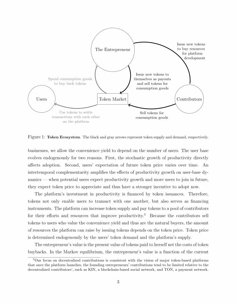
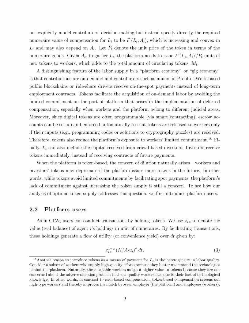
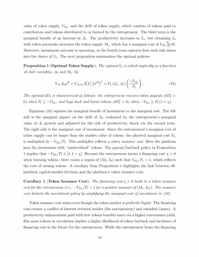
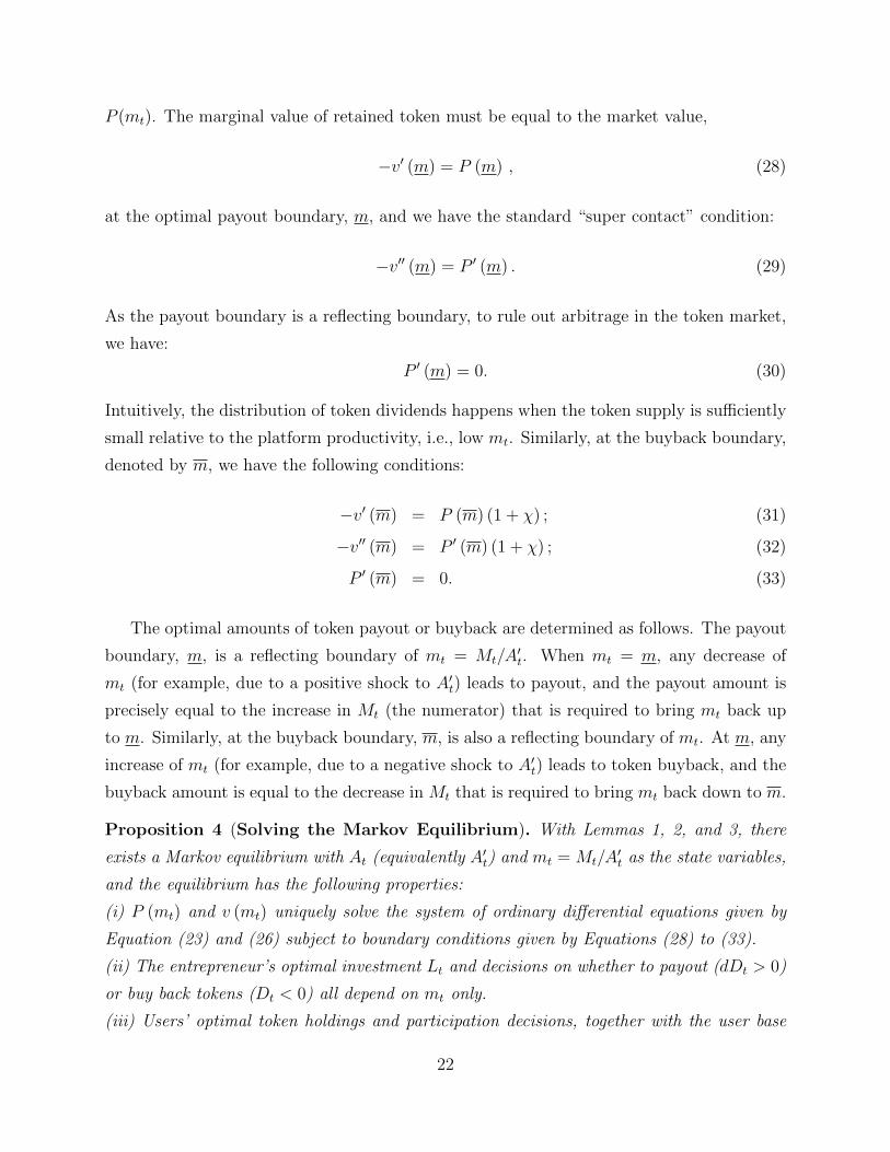
Users Token Market

The Entrepreneur

Contributors

Use tokens to settletransactions with each other

on the platform

Issue new tokens tothemselves as payouts

and sell tokens forconsumption goods

Spend consumption goodsto buy back tokens

Issue new tokensto buy resources

for platformdevelopment

Sell tokens forconsumption goods

Figure 1: Token Ecosystem. The black and gray arrows represent token supply and demand, respectively.

businesses, we allow the convenience yield to depend on the number of users. The user base

evolves endogenously for two reasons. First, the stochastic growth of productivity directly

affects adoption. Second, users’ expectation of future token price varies over time. An

intertemporal complementarity amplifies the effects of productivity growth on user-base dy-

namics — when potential users expect productivity growth and more users to join in future,

they expect token price to appreciate and thus have a stronger incentive to adopt now.

The platform’s investment in productivity is financed by token issuances. Therefore,

tokens not only enable users to transact with one another, but also serves as financing

instruments. The platform can increase token supply and pay tokens to a pool of contributors

for their efforts and resources that improve productivity.5 Because the contributors sell

tokens to users who value the convenience yield and thus are the natural buyers, the amount

of resources the platform can raise by issuing tokens depends on the token price. Token price

is determined endogenously by the users’ token demand and the platform’s supply.

The entrepreneur’s value is the present value of tokens paid to herself net the costs of token

buybacks. In the Markov equilibrium, the entrepreneur’s value is a function of the current

5Our focus on decentralized contributions is consistent with the vision of major token-based platformsthat once the platform launches, the founding entrepreneurs’ contributions tend to be limited relative to thedecentralized contributors’, such as KIN, a blockchain-based social network, and TON, a payment network.

3

platform productivity and token supply, which are the two state variables. The marginal

value of productivity is positive, capturing the equilibrium dynamics of users’ adoption and

valuation of tokens. The marginal value of token supply is negative due to the downward

pressure of supply on token price and the entrepreneur’s token payout. In order to protect

the continuation value (i.e., the present value of future token payout), the entrepreneur may

even find it optimal to buy back tokens (through external financing) and burn them out of

circulation.6 In equilibrium, the entrepreneur receives token payout when token supply is

low relative to platform productivity and buys back tokens when token supply is relatively

high. Figure 1 summarizes the circulation of tokens in our dynamic platform economy.7

A key friction in our model is that when buying back tokens, the entrepreneur has to raise

costly external funds. While token buybacks occur occasionally, the associated financing

cost propagates into a dynamic token issuance cost in every state of the world because

every time more tokens are issued, the entrepreneur’s expectation of costly future buyback

changes accordingly. Specifically, the entrepreneur’s cost of issuing one more token (i.e., the

marginal decline of continuation value) is larger than the market price of tokens (i.e., the

users’ valuation of tokens). This wedge causes the platform to under-invest in productivity.

In our model, tokens are perfectly liquid. For example, newly issued tokens are not subject

to discounts due to informational asymmetry. They are simply valued by the marginal user’s

indifference condition. Despite the perfect liquidity, tokens are not immune to financial

frictions. The token issuance cost emerges because the entrepreneur’s optimal buyback

relies on costly external funds. In other words, the optimal strategy of token management

transmits the traditional costs of external financing into an endogenous cost of token issuance.

The dynamic token issuance cost implies a conflict of interest between the entrepreneur

and users. Productivity enhancement paid with tokens benefits users via a higher convenience

yield. But more tokens in circulation implies a higher likelihood of costly token buyback in

the future. Therefore, while the entrepreneur bears the costs of future token buyback, the

benefits of token-financed investment are shared with users. Admittedly, part of such benefits

flow to the entrepreneur through a higher token price (and higher value of token payout),

but the entrepreneur cannot seize all surplus from users. Users are heterogeneous in deriving

6Burning tokens means sending them to a public “eater address” from which they can never be retrievedbecause the address key is unobtainable. Practitioners often burn tokens to boost token price and rewardtoken holders (e.g., Binance and Ripple). Some also use Proof-of-Burn as an environmentally friendlyalternative to Proof-of-Work to generate consensus (e.g., Counterparty (XCP) blockchain), or destroy unsoldtokens or coins after an ICO or seasoned token issuances for fair play (e.g., Neblio’s burning of NEBL tokens).

7We thank our discussant Sebastian Gryglewicz for sharing this figure with us in his discussion slides.

4

convenience yield from tokens, so only the marginal user breaks even while those who derive

more convenience yield enjoy a positive surplus.8 Token overhang, which is underinvestment

due to the surplus leakage to users, is a fundamental feature of token-based financing.

After characterizing the optimal token-management strategy (i.e., investment, payout,

and buyback), we analyze the value of introducing blockchain technology in our setting.

Blockchains distinguish themselves from traditional technologies in several aspects: im-

mutable record keeping due to time-stamping and linked-list data structure, smart con-

tracting for automating and ensuring execution, and distributed design for easier monitoring

and decentralized governance. These features enable the commitment of predetermined

token-supply rules that, we show, are valuable in addressing the underinvestment problem.

Specifically, motivated by Ethereum, we consider a constant rate of token issuances that

finance investment. We find that commitment mitigates the underinvestment problem by

severing the state-by-state linkage between investment and the token issuance cost. While

the increased amount of tokens issued for investment results in more frequent costly token

buyback, the entrepreneur’s value is higher than the case with discretionary token supply,

because the token price is higher under faster trajectories of productivity and user-base

growth. Previous studies of tokens assume predetermined rules of supply. In contrast, our

analysis starts from the fully discretionary supply of tokens. By comparing the discretionary

case with the predetermined case, we are able to identify the value-added of commitment and

to partly explain the popularity of blockchain technology among the platform businesses.

Finally, our model also has implications for the design of stablecoins. Different from the

approaches based on collateralization, the entrepreneur in our setting supports the franchise

value by occasionally buying back tokens out of circulation. When the token supply is high

relative to the platform productivity — precisely at the moment that token price is low but

the marginal value of reducing token supply is high — the buyback happens. The resulting

token supply dynamics moderate the token price fluctuations. Therefore, for platforms with

endogenous productivity growth, their tokens are inherently stable.

Overall, our model sheds light on the equilibrium dynamics of token-based communities

and also provides a guiding framework for practitioners. The various token offering schemes

observed in practice can be viewed as special (suboptimal) cases. Appendix A discusses the

institutional background and offers a rich set of real-life examples.

8The intuition is related to the surplus that a monopolistic producer forgoes to consumers when pricediscrimination is impossible. Here tokens are traded at a prevailing price among competitive users, so theentrepreneur cannot extract more value from users who derive a higher convenience yield from tokens.

5

Literature. The paper that is most related to ours is Gryglewicz, Mayer, and Morellec

(2020) who also study endogenous platform productivity but focus on the founders’ efforts,

rather than decentralized contributors’ efforts and resources. Mayer (2020) further introduces

speculators and studies the conflict of interest among various token holders. Our paper

differs in our focus on tokens as a means of payment and on a different stage of platform life-

cycle. Gryglewicz, Mayer, and Morellec (2020) model uncertainty in the exogenous arrival of

platform launching and a constant token price post-launch. We study a post-launch platform

with uncertainty from Brownian productivity shocks, and model the endogenous fluctuation

of token price. Finally, while they consider a fixed token supply, we characterize the optimal

state-contingent supply and highlight the value of commitment brought by blockchains.

Our paper connects the literature on platform economics to dynamic corporate finance,

especially the studies emphasizing the role of financial slack and issuance costs (e.g., Bolton,

Chen, and Wang, 2011; Hugonnier, Malamud, and Morellec, 2015; Decamps, Gryglewicz,

Morellec, and Villeneuve, 2016). Instead of cash management, we analyze platforms’ token-

supply management when investment induces user network effects and, importantly, the

token price varies endogenously as users respond to supply variation.9 From a methodological

perspective, our paper is related to Brunnermeier and Sannikov (2016) and Li (2017), who

both study the endogenous price determination of inside money (deposits) issued by banks.

The key distinction is that tokens are outside money instead of liabilities of the platforms.

Our paper contributes to the broad literature on digital platforms. Studies on traditional

platforms (e.g., Rochet and Tirole, 2003) do not consider the use of tokens as platforms’

native currencies (local means of payment).10 We share the view on platform tokens with

Brunnermeier, James, and Landau (2019): a platform is a currency area where a unique set

of economic activities take place and its tokens derive value by facilitating the associated

transactions.11 Beyond this, we emphasize that a platform can invest in its quality, for

example, payment efficiency (Duffie, 2019), thereby raising token value. We are the first to

formally analyze how platforms manage their investment and payout through token supply,

and provide insights into the incentives and strategies of platform businesses.

Our paper adds to emerging studies on blockchains and cryptocurrencies. We innovate

upon CLW by endogenizing token supply and incorporating the entrepreneur’s long-term

interests (franchise value), which allows us to explore new issues concerning the dynamics of

9Related to Cagan (1956), the entrepreneur essentially maximizes the present value of seigniorage flows.10Stulz (2019) reviews the recent financial innovations by major digital platforms.11Our model differs from the majority of monetary-policy models because token issuance finances invest-

ment, as in Bolton and Huang (2017), and payout rather than to stimulate nominal aggregate demand.

6

optimal platform investment and financing, the conflict of interest between the entrepreneur

and users, and the role of blockchain technology in platform economics.12 By doing so,

we are able to provide the first unified theory of dynamic corporate finance of post-launch

platforms: optimal monetary, investment, and payout policies with both token price and

user base being endogenously determined. We also demonstrate the commitment value of

blockchains.13 Hinzen, John, and Saleh (2019) show that limited adoption is an equilibrium

outcome in Proof-of-Work (PoW) blockchains and Irresberger, John, and Saleh (2019) em-

pirically document that Proof-of-Stake (PoS) blockchains dominate on adoption scale. Our

focus is on the use of tokens for platform finance and endogenous adoption, regardless of the

consensus protocol and level of decentralization issues we explore in CLW.

Furthermore, our paper adds to the discussion on token price volatility and stablecoins.

On the demand side, high token price volatility could be an inherent feature of platform

tokens due to technology uncertainty and endogenous user adoption (see CLW).14 Saleh

(2018) emphasizes that token supply under proof-of-burn (PoB) protocols can reduce price

volatility. We endogenize both the demand for tokens driven by users’ transaction needs and

dynamic adoption, and the supply of tokens for platform development and the founders’ rent

extraction. We show that the optimal token supply strategy stabilizes token price.

Finally, our paper is broadly related to the literature on crowdsourcing and the gig

economy. Blockchain-based consensus provisions in the form of cryptocurrency mining and

resources (capital) raised via initial coin offerings (ICOs) are salient examples of decen-

tralized on-demand contributions. Existing studies on ICOs and crowdfunding focus on

one-time issuance of tokens before the platform launches (e.g., Canidio, 2018; Garratt and

Van Oordt, 2019; Chod and Lyandres, 2018), yet platforms increase token supply on an on-

going basis. Existing studies also center around the founders’ hidden efforts or asymmetric

information pre-launch, whereas we emphasize decentralized contributors’ effort post-launch

that is highly relevant for digital platforms and the gig economy.15 This distinction is a key

12The studies on the design issues of tokens (e.g., proof-of-work protocols) typically assume a fixed userbase (e.g., Chiu and Wong, 2015; Chiu and Koeppl, 2017). A fixed token supply is a common feature amongthe models that examine the roles of tokens among users and contributors (e.g., miners in Sockin and Xiong,2018; Pagnotta, 2018) and the existing models of token valuation (e.g., Fanti, Kogan, and Viswanath, 2019).

13Even though commitments through tokens can be valuable in various settings (e.g., Goldstein, Gupta,and Sverchkov, 2019), in practice, the reliability of blockchain and the associated commitment value arenot free of costs (Abadi and Brunnermeier, 2018). As analyzed by Biais, Bisiere, Bouvard, and Casamatta(2019), proof-of-work protocols can lead to competing records of transactions (“forks”). Commitment isoften implemented via smart contracts, for which Cong and He (2019) provide some examples.

14Hu, Parlour, and Rajan (2018) and Liu and Tsyvinski (2018) document token price dynamics empirically.15The entrepreneurs in the ICO models do not engage in dynamic token management for long-term platform

7

consideration in determining whether tokens are securities or not based on the Howey test.16

2 Model

Three types of agents interact in a continuous-time economy: an entrepreneur (used

interchangeably with “platform owners”), a pool of contributors, and a unit measure of users.

The entrepreneur, representing the group of platform founders, key personnel, and venture

investors, designs the platform’s protocol. Contributors, who represent individual miners

(transaction ledger keepers), third-party app developers, and other providers of on-demand

labor in practice, devote efforts and resources required for the operation and continuing

development of the platform. Users conduct peer-to-peer transactions and realize trade

surpluses on the platform. A generic consumption good serves as the numeraire.

2.1 Platform productivity and contributors

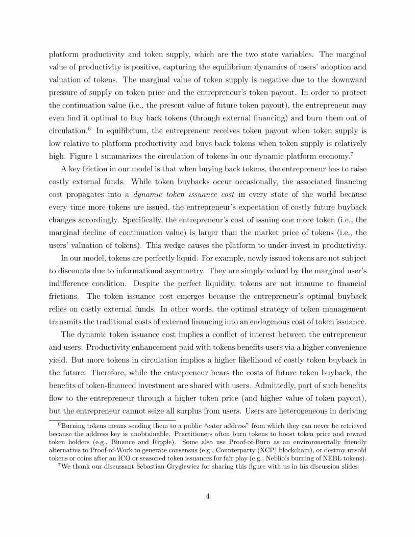
We study a dynamically evolving platform whose productivity (synonymous with qual-

ity), At, evolves as follows:dAtAt

= LtdHt, (1)

where Lt is the decentralized contribution (contributors’ resources and labor as described

in Appendix A) the entrepreneur gathers through token payments to grow At. dHt is an

investment efficiency shock,

dHt = µHdt+ σHdZt. (2)

Here Zt is a standard Brownian motion that generates the information filtration.17 At

broadly captures marketplace efficiencies, network security, processing capacity, regulatory

conditions, users’ interests, the variety of activities feasible on the platform, etc. It therefore

affects directly users’ utility on the platform, which shall be made clear below.

Our focus is on the dynamic interaction between the entrepreneur and users, so we do

development, and thus, do not concern the franchise value. Despite newly issued tokens from platforms,decentralized contributors such as miners can also receive transaction fees (Basu, Easley, O’Hara, and Sirer,2019; Easley, O’Hara, and Basu, 2019; Huberman, Leshno, and Moallemi, 2019; Lehar and Parlour, 2020).

16For example, the SEC sued Telegram/TON that raised US$1.7 billion through a private placementfor not complying with securities laws (Michaels, 2019). The issue boils down to whether token investorspost-launch expect to profit from the entrepreneurs’ effort or decentralized contributions.

17The process Ht may result from the entrepreneur’s efforts prior to platform launch, which we take asexogenous to differentiate our model from models on founders’ efforts as discussed in the literature review.

8

not explicitly model contributors’ decision-making but instead specify directly the required

numeraire value of compensation for Lt to be F (Lt, At), which is increasing and convex in

Lt and may also depend on At. Let Pt denote the unit price of the token in terms of the

numeraire goods. Given At, to gather Lt, the platform needs to issue F (Lt, At) /Pt units of

new tokens to workers, which adds to the total amount of circulating tokens, Mt.

A distinguishing feature of the labor supply in a “platform economy” or “gig economy”

is that contributions are on-demand and contributors such as miners in Proof-of-Work-based

public blockchains or ride-share drivers receive on-the-spot payments instead of long-term

employment contracts. Tokens facilitate the acquisition of on-demand labor by avoiding the

limited commitment on the part of platform that arises in the implementation of deferred

compensation, especially when workers and the platform belong to different judicial areas.

Moreover, since digital tokens are often programmable (via smart contracting), escrow ac-

counts can be set up and enforced automatically so that tokens are released to workers only

if their inputs (e.g., programming codes or solutions to cryptography puzzles) are received.

Therefore, tokens also reduce the platform’s exposure to workers’ limited commitment.18 Fi-

nally, Lt can also include the capital received from crowd-based investors. Investors receive

tokens immediately, instead of receiving contracts of future payments.

When the platform is token-based, the concern of dilution naturally arises – workers and

investors’ tokens may depreciate if the platform issues more tokens in the future. In other

words, while tokens avoid limited commitments by facilitating spot payments, the platform’s

lack of commitment against increasing the token supply is still a concern. To see how our

analysis of optimal token supply addresses this question, we first introduce platform users.

2.2 Platform users

As in CLW, users can conduct transactions by holding tokens. We use xi,t to denote the

value (real balance) of agent i’s holdings in unit of numeraires. By facilitating transactions,

these holdings generate a flow of utility (or convenience yield) over dt given by:

x1−αi,t (Nγt Atui)

α dt, (3)

18Another reason to introduce tokens as a means of payment for Lt is the heterogeneity in labor quality.Consider a subset of workers who supply high-quality efforts because they better understand the technologiesbehind the platform. Naturally, these capable workers assign a higher value to tokens because they are notconcerned about the adverse selection problem that low-quality workers face due to their lack of technologicalknowledge. In other words, in contrast to cash-based compensation, token-based compensation screens outhigh-type workers and thereby improves the match between employer (the platform) and employees (workers).

9

where Nt is the platform user base, ui captures agent i’s needs for platform transactions, and

α, γ ∈ (0, 1) are constants. Similar to CLW, we provide a theoretical foundation in Appendix

B. A crucial difference from CLW is that we endogenize At and the token supply Mt.

The flow utility of token holdings depends on Nt, the total measure of users on the plat-

form with xi,t > 0.19 This specification captures the network externality among users, such

as the greater ease of finding trading or contracting counterparties in a larger community.

We allow users’ transaction needs, ui, to be heterogeneous. Let Gt (u) and gt (u) de-

note the cross-sectional cumulative distribution and density function respectively that are

continuously differentiable over a positive support [U t, U t]. ui can be broadly interpreted:

For payment blockchains (e.g., Ripple and Bitcoin), a high value of ui reflects user i’s needs

for international remittance. For smart-contracting platforms (e.g., Ethereum), ui captures

user i’s project productivity, and token holdings facilitate contracting.20 In decentralized

computation (e.g., Dfinity) and data storage (e.g., Filecoin) applications, ui corresponds to

the need for secure and fast access to computing power and data.

Recall that Pt denotes the unit price of a token in terms of the numeraire. Let ki,t denote

the number of tokens that user i holds, then the real balance is:

xi,t = Ptki,t. (4)

To join the platform (i.e., ki,t > 0), a user incurs a flow cost φdt. For example, transacting

on the platform requires attention; account maintenance and data migration also take effort.

Therefore, only agents with sufficiently high ui choose to join the platform.

Let yi,t denote user i’s cumulative utility from platform activities. We follow CLW and

assume that the users are well-diversified so that their transaction surpluses and financial

gains on the platform are priced by an exogenous stochastic discount factor. Thus, we can

interpret the equilibrium dynamics as dynamics under the risk-neutral measure. When users

are risk neutral, the risk-neutral measure coincides with the data-generating probability

19One example involves a producer who accepts tokens as a means of payment and earns net profits equalto the full transaction surplus. The profits depend on the scale of operation, i.e., the sales xi,t, and variablesthat determine the profit margin, which include the total customer outreach, Nt, the platform efficiency At,and the producer’s idiosyncratic productivity ui.

20For example, in a debt contract, the borrower’s Ethereum can be held in an escort or “margin” account,which is automatically transferred to the lender in case of default. Posting more Ethereum as margin allowsfor larger debt contracts, which in turn lead to projects of larger scale and profits.

10

(physical measure). The user i’s objective is given by:

E[∫ ∞

0

e−rtdyi,t

], (5)

where the incremental utility dyi,t is:

dyi,t = max

{0, max

ki,t>0

[(Ptki,t)

1−α (Nγt Atui)

α dt+ ki,tEt [dPt]− φdt− Ptki,trdt]}

. (6)

The outer “max” operator in (6) reflects user i’s option to leave and obtain zero surplus

from platform activities, and the inner “max” operator reflects user i’s optimal choice of ki,t.

Inside the inner max operator are four terms that give the incremental transaction surpluses

from platform activities. The first corresponds to the payment convenience yield given in

(3). The second is the expected capital gains from holding ki,t units of tokens. The third is

the participation cost and the last term is the financing) cost of holding ki,t units of tokens.

It is worth emphasizing that platform users must hold tokens for at least an instant,

dt, to complete transactions and derive utility flows, and are therefore exposed to token

price change over dt. Appendix A contains motivating examples and institutional details.

We implicitly assume a liquid secondary market for tokens. Hence, after receiving tokens,

decentralized contributors can immediately sell tokens to users. Contributors can also be

users themselves, and the model is not changed at all as long as the utility from token usage

and the disutility from contributing Lt (which gives rise to F (·)) are additively separable.

2.3 The entrepreneur

We refer to the founding entrepreneurs, the key developers, and initial investors who

own the platform collectively as the entrepreneur. Importantly, the entrepreneur designs

the platform protocols and determines the investment strategies {Lt, t ≥ 0}. Over time, the

entrepreneur receives a cumulative number of tokens Dt as dividends and, similar to users,

evaluates the tokens with a risk-neutral objective function and discount rate r:

max{Lt,Dt}t≥0

∫ +∞

t=0

E[e−rtPtdDt

[I{dDt≥0} + (1 + χ) I{dDt<0}

]]. (7)

11

When dDt > 0, the entrepreneur receives token dividends that have a market value Pt

per unit, as a form of compensation for his essential human capital.21 Note that token

dividends could be either continuous (i.e., of dt order) or lumpy, and that in equilibrium,

the entrepreneur immediately sells her tokens to users who are the natural buyers of tokens

because they derive an extra convenience yield from token holdings.

We allow the entrepreneur to buy back and burn tokens to reduce the token supply (i.e.,

dDt < 0). When dDt < 0, the entrepreneur raises external financing (numeraire goods) at

a proportional cost χ for token buyback.22 By reducing token supply, the entrepreneur can

boost token price, and consequently increase the value of future token dividends. A higher

token price also allows the platform to gather more resources for productivity growth. We

allow the amount of token buyback to be continuous (i.e., of dt order) or lumpy.

The key accounting identity that describes the evolution of token supply entails both the

tokens issued for financing platform investment and the entrepreneur’s dividend/buyback:

dMt =F (Lt, At)

Ptdt+ dDt. (8)

When the platform invests (the first term on the right side) or distributes token dividends

(dDt > 0), the total amount of tokens in circulation increases; the token supply decreases

when the entrepreneur burns tokens out of circulation (dDt < 0).23 In the next section, we

show that the entrepreneur’s financial slack decreases in Mt. An increase in Mt depresses

token price Pt, so whenMt rises to a sufficiently high level, the entrepreneur, who is concerned

over the value of future token payouts (i.e., the continuation value), pays the financing cost

to raise funds for token buyback that token price. Therefore, under the financing cost χ,

managing the token stock is akin to managing cash inventory in Bolton, Chen, and Wang

(2011) and Hugonnier, Malamud, and Morellec (2015). A firm’s financial slack increases in

its cash holdings, because when its cash dries up, the firm has to resort to costly external

21For example, blockchain behemoth Bitmain Technologies Ltd and Founders Fund (known for early betson SpaceX and Airbnb) invest in EOS and hold ownership stakes that entitle them to future token rewards.The gradual distribution of token dividends can be viewed as contingent vesting in reality – a certain amountof total tokens Dt have been allocated by time t but are distributed over time (via dDt) depending on thestages of platform development and the tokens outstanding (i.e., different values of At and Mt).

22The external financing cost assumption (via parameter χ) is in line with those in the corporate financeliterature, e.g., Bolton, Chen, and Wang (2011) and Hugonnier, Malamud, and Morellec (2015), who modelin reduced form information, incentive, and transactions costs of raising external funds.

23It is suboptimal for the platform to pay contributors with costly external financing. Instead, it isgenerally optimal to use tokens (internal financing) to compensate contributors as doing so delays incurringthe costs of external financing. However, using tokens as internal funds incurs a shadow cost because anincrease in token supply depresses token price, which reduces the entrepreneur’s token payout value.

12

funds. In our model, the financial slack decreases in token supply, because when the token

supply rises too high, the entrepreneur has to buy back tokens with costly external funds.

In what follows, we characterize a Markov equilibrium. The two state variables are the

productivity At, which measures the technological aspect of the platform, and the token

supply Mt, which inversely measures the financial slack.

Definition 1. A Markov equilibrium with state variable At and Mt is comprised of agents’

decisions and token price dynamics, such that the token market-clearing condition holds,

users optimally decide to participate (or not) and choose token holdings, contributors supply

resources for the compensation of F (Lt, At) in numeraire value, and the platform strategies,

i.e., Lt and Dt, are optimally designed to maximize the entrepreneur’s value.

3 Dynamic equilibrium

We first derive the entrepreneur’s optimal investment and token payout and buyback,

which in turn pin down the token supply. We then derive platform users’ optimal decisions

on adoption and token holding in order to aggregate token demand. Finally, token market

clearing yields the equilibrium dynamics of token price.

3.1 Optimal token supply

At time t, the entrepreneur’s continuation or franchise value Vt (i.e., the time-t value

function) satisfies the following Hamilton–Jacobi–Bellman (HJB) equation:

rV (Mt, At) dt = maxLt,dDt

PtdDt

[I{dDt≥0} + (1 + χ) I{dDt<0}

]+ VMt

[F (Lt, At)

Ptdt+ dDt

]+ VAtAtLtµ

Hdt+1

2VAtAtA

2tL

2t (σ

H)2dt . (9)

The first term in this HJB equation reflects the dividend payout (dDt > 0) and buyback

(dDt < 0). When there are more tokens in circulation, the token price is depressed and

the entrepreneur’s continuation value is reduced. Therefore, we expect VMt < 0, which we

later confirm in the numerical solution. Payout occurs only if −VMt ≤ Pt, i.e., the market

value of token weakly exceeds the marginal cost of increasing token supply. Token buyback

happens when −VMt ≥ Pt (1 + χ), i.e., the marginal benefit of decreasing token supply is

not lower than the cost of burning tokens. The second term is the product of the marginal

13

value of token supply, VMt , and the drift of token supply, which consists of tokens paid to

contributors and tokens distributed to or burned by the entrepreneur. The third term is the

marginal benefit of an increase in At. The productivity increases in Lt, but obtaining Lt

with token payments increases the token supply Mt, which has a marginal cost of VMt

FLtPtdt.

Moreover, investment outcome is uncertain, so the fourth term captures how such risk enters

into the choice of Lt. The next proposition summarizes the optimal policies.

Proposition 1 (Optimal Token Supply). The optimal Lt is solved implicitly as a function

of state variables, At and Mt, by

VAtAtµH + VAtAtA

2tL∗t

(σH)2

= FL (L∗t , At)

(−VMt

Pt

). (10)

The optimal dDt is characterized as follows: the entrepreneur receives token payouts (dD∗t >

0) when Pt ≥ −VMt, and buys back and burns tokens (dD∗t < 0) when −VMt ≥ Pt (1 + χ).

Equation (10) equates the marginal benefit of investment to the marginal cost. The left

side is the marginal impact on the drift of At, evaluated by the entrepreneur’s marginal

value of At growth and adjusted for the risk of productivity shock via the second term.

The right side is the marginal cost of investment. Since the entrepreneur’s marginal cost of

token supply can be larger than the market value of tokens, the physical marginal cost FL

is multiplied by −VMt/Pt. This multiplier reflects a token issuance cost. Here the platform

pays for investment with “undervalued” tokens. The payout/buyback policy in Proposition

1 implies that −VMt/Pt ∈ [1, 1 + χ]. Because the entrepreneur incurs a financing cost χ > 0

when burning tokens, there exists a region of (Mt, At) such that VMt/Pt > 1, which reflects

the cost of issuing tokens. A corollary from Proposition 1 highlights the link between off-

platform capital-market frictions and the platform’s token issuance cost:

Corollary 1 (Token Issuance Cost). The financing cost χ > 0 leads to a token issuance

cost for the entrepreneur (i.e., −VMt/Pt > 1 for a positive measure of (Mt, At)). The issuance

cost distorts the investment policy by amplifying the marginal cost of investment in (10).

Token issuance cost arises even though the token market is perfectly liquid. The financing

cost creates a conflict of interest between insider (the entrepreneur) and outsiders (users). A

productivity enhancement paid with new tokens benefits users via a higher convenience yield.

But more tokens in circulation implies a higher likelihood of token buyback and incidence of

financing cost in the future for the entrepreneur. While the entrepreneur bears the financing

14

cost, the benefits are shared with users. Admittedly, as the token demand strengthens

following a productivity increase, the entrepreneur benefits from a higher token price (and

higher value of token payout), but the entrepreneur cannot capture the full surplus.

Users are heterogeneous in deriving convenience yield from tokens, so only the marginal

user breaks even after token price increases, while those who derive more convenience yield

capture a positive surplus. The intuition is similar to that in a monopolistic producer’s

problem when full price discrimination is impossible. Here tokens are traded at a prevailing

price among competitive users, so the entrepreneur cannot extract more value from users

who derive a higher convenience yield than the marginal token holder.

As such, token-based financing naturally exhibits token overhang, which is underinvest-

ment due to the leakage of surplus to users. Uncertainty also plays a critical role here.

Without dZt, the productivity shock, Lt, always increases At. Then, with a sufficiently ef-

ficient investment technology F (·) (so that relatively few new tokens are needed to pay for

Lt), we arrive at a situation where, following investment, At always grows faster than Mt.

As we will show below, the entrepreneur conducts costly token buyback when Mt is too high

relative to At. Thus, with At always growing faster than Mt, the entrepreneur always moves

away from costly token buyback after making investment. As a result, the financing cost is

never a concern given this sufficiently efficient F (·). However, in the presence of uncertainty

in investment outcome, there always exists a probability that Mt increases faster than At

after investment, moving the platform closer to costly buyback.

In sum, the mechanism of token overhang relies on three ingredients in the model. First,

when the entrepreneur raises consumption goods to buy tokens out of circulation, the en-

trepreneur faces a financing cost. Second, users are heterogeneous in deriving convenience

yield from token holdings, so under a single token price that clears the competitive market,

only the marginal user breaks even. Third, the outcome of platform investment is uncertain.

The first ingredient creates a private cost of investment for the entrepreneur, and the second

implies a surplus leakage to users. Together, they generate a conflict of interest between the

entrepreneur and users. Finally, the third ingredient, uncertainty, is needed so that despite

the specification of F (·), token overhang always exists.

Our characterization of the optimal investment and payout/buyback policies in some

sense allays the concern over fraudulent designs or manipulations by the founding developers,

for example, through building “back doors” in the protocol to steal tokens and depress the

token price when selling the stolen tokens in secondary markets. As shown in Proposition

1, our setup allows the entrepreneur to extract tokens as dividends, and the optimal payout

15

policy already maximizes the entrepreneur’s value. In other words, the policy is incentive-

compatible in this subgame perfect equilibrium between a large player (the entrepreneur)

and a continuum of small players (users). From a regulatory perspective, a proposal of

blockchain or platform design should disclose the policy of token payout to the platform

owners, and it should be broadly in line with the above characterization.

3.2 Aggregate token demand

We conjecture and later verify that in equilibrium, the token price, Pt, evolves as

dPt = PtµPt dt+ Ptσ

Pt dZt, (11)

where µPt and σPt are endogenously determined. Agents take the price process as given under

rational expectation. Conditioning on joining the platform, user i chooses the optimal token

holdings, k∗i,t, by using the following first-order condition,

(1− α)

(Nγt AtuiPtk∗i,t

)α+ µPt = r, (12)

which states that the sum of marginal transaction surplus on the platform and the expected

token price change is equal to the required rate of return, r.

Rearranging this equation, we obtain the following expression for optimal token holdings:

k∗i,t =Nγt AtuiPt

(1− αr − µPt

) 1α

. (13)

k∗i,t has several properties. First, users hold more tokens when the common productivity, At,

or user-specific transaction need, ui, is high, and also when the user base, Nt, is larger due

to network effects. Equation (13) reflects an investment motive to hold tokens, that is k∗i,t

increases in the expected token appreciation, µPt .

Using k∗i,t, we obtain the following expression for the user’s maximized profits conditional

on participating on the platform:

Nγt Atuiα

(1− αr − µPt

) 1−αα

− φ. (14)

User i only participates when the preceding expression is non-negative. That is, only those

16

users with sufficiently large ui participate. Let ut denote the type of the marginal user, then

ut = u(Nt;At, µ

Pt

)=

φ

Nγt Atα

(r − µPt1− α

) 1−αα

. (15)

The adoption threshold ut decreases in At because a more productive platform attracts more

users. The threshold also decreases when users expect a higher token price appreciation (i.e.,

higher µPt ). Because only agents with ui ≥ ut participate, the user base is then:

Nt = 1−Gt (ut) . (16)

Equations (15) and (16) jointly determine the user base Nt given At and µPt .24

Proposition 2 (Token Demand and User Base). Given At and µPt , the platform has a

positive user base when Equations (15) and (16) have solutions for ut and Nt. Conditional

on participating, user i’s optimal token holding, k∗i,t, is given by Equation (13). The token

holding, k∗i,t, decreases in Pt and increases in At, µPt , ui, and Nt.

3.3 Token market clearing

Clearing the token market pins down the token price. We define the participants’ aggre-

gate transaction need by aggregating ui of participating users:

Ut :=

∫u≥ut

ugt (u) du. (17)

The market-clearing condition is:

Mt =

∫i∈[0,1]

k∗i,tdi. (18)

Substituting optimal holdings in Equation (13) into the market-clearing condition in Equa-

tion (18), we arrive at the token pricing formula in Proposition 3.

Proposition 3 (Token Pricing). The equilibrium token price is given by

Pt =Nγt UtAtMt

(1− αr − µPt

) 1α

. (19)

24We do not consider the trivial solution of zero adoption, which always leads to a zero token price.

17

Token price increases in Nt. The larger the user base is, the higher the trade surplus in-

dividual participants can realize by holding tokens, and the stronger the token demand. The

price-to-user base ratio increases in the productivity, the expected price appreciation, and

the network participants’ aggregate transaction need, while it decreases in the token supply

Mt.25 Equation (19) implies a differential equation for Pt in the state space of (Mt, At). This

can be clearly seen once we apply the infinitesimal generator to Pt = P (Mt, At), expressing

µPt into a collection of first and second derivatives of Pt by Ito’s lemma. Note that the equilib-

rium user base, Nt, is already a function of At and µPt as shown in Proposition (2). Therefore,

the collection of token market-clearing conditions at every t essentially characterize the full

dynamics of token price. This method of solving token price follows CLW.

Equations (8) and (18) describe the primary and secondary token markets. The change

of Mt is a flow variable, given by Equation (8), that includes the new issuances from platform

investment and payout and the repurchases by the entrepreneur. The token supply Mt is a

stock variable, and through Equation (18), it equals the token demand of users.

Discussion: Durable-good monopoly. The problem faced by a token-based platform

reminisces a durable-good monopoly problem (e.g., Coase, 1972; Stokey, 1981; Bulow, 1982).

First, token issuance permanently increases the supply. When issuing tokens to finance

investment or payout, the entrepreneur is competing with future selves. Second, given a zero

physical cost of creating tokens, the Coase intuition seems applicable: The entrepreneur can

be tempted to satisfy the residual demand by ever lowering token price as long as the price

is positive (i.e., above the marginal cost of production). Thus, users wait for lower prices,

driving token price to zero. Our model differs from the Coasian setting in two aspects. First,

even though the physical cost of producing tokens is zero, the dynamic token issuance cost

increases in the token supply as we show in the next section. This reminisces the result in

Kahn (1986) that the Coase intuition does not hold in the presence of increasing marginal

cost of production. Second, in contrast to theories of durable-good monopoly, token demand

in our model is not stationary; in fact, it increases geometrically with the endogenously

growing At, so users cannot expect lower token price in the future. Therefore, we can solve

an equilibrium with a positive token price in the next section.

25The formula reflects certain observations by practitioners, such as incorporating DAA (daily activeaddresses) and NVT Ratio (market cap to daily transaction volume) in token valuation framework, butinstead of heuristically aggregating such inputs into a pricing formula, we solve both token pricing and useradoption as an equilibrium outcome. See, for example, Today’s Crypto Asset Valuation Frameworks byAshley Lannquist at Blockchain at Berkeley and Haas FinTech.

18

4 Equilibrium characterization

We further characterize the equilibrium by analytically deriving and numerically solving

the system of differential equations concerning token price and the entrepreneur’s value

function. To streamline exposition and focus on core economic insights, we make some

intuitive parametric assumptions.

4.1 User distribution and investment cost function

We assume that ui follows the commonly used Pareto distribution on [U t,+∞) with

cumulative probability function (c.d.f.) given by the Pareto distribution:

Gt (u) = 1−(U t

u

)ξ, (20)

where ξ > 1 and U t = 1/ (ωAκt ) , ω > 0, κ ∈ [0, 1]. The cross-section mean of ui isξUtξ−1 .

It is assumed that U t decreases in At, which reflects the competition from follower plat-

forms inspired by the success (high At) of the platform in question. For example, after the

success of Bitcoin, alternative blockchains emerge as competitors in the area of payments.

Similarly, there are alternative platforms to Ethereum for smart contracting. The overall

effects of competition depend on the parameters ω and κ, while the parameter ξ governs

how heterogeneous users transaction needs (ui) are (i.e., the dispersion of ui distribution).

Lemma 1 (Parameterized User Base). Given At and µPt , from Proposition 2, we have

a unique non-degenerate solution, Nt, from Equations (15) and (16), given by:

Nt = A′t

(α

ωφ

) ξ1−ξγ

(1− αr − µPt

)( ξ1−ξγ )( 1−α

α ), where A′t ≡ A

(1−κ)( ξ1−ξγ )

t , (21)

if ut ≥ 1ωAκt

, i.e., A1−κt ( 1−α

r−µPt)1−αα ≤ ωφ

α; otherwise, Nt = 1.

A′t is a transformed version of At. It is the effective productivity that captures user ho-

mogeneity, platform competition, and user network effects. Intuitively, the way productivity

matters is amplified by the network-effect parameter γ (introduced in (3)) but dampened

by the competition parameter κ. When there is no network effect (γ = 0) or competition

(κ = 0), the exponent is simply ξ, which measures user heterogeneity. The effect of user

heterogeneity has two components. One is the interaction component with γ, as seen in the

19

denominator of ξ1−ξγ . When agents are more homogeneous (larger ξ), small changes in At

brings big changes in adoption, which is amplified by network effects. The second compo-

nent is in the numerator of ξ1−ξγ . Even without the network effect, greater homogeneity still

means that there is a bigger adoption sensitivity with respect to platform productivity.

Our later discussion focuses on ξγ < 1, so that the user base, Nt, increases in the platform

productivity despite platform competition. This is realistic because a technology leader

usually benefits from its innovation despite the presence of competing followers. Moreover,

we focus on low values of At, such that Nt < 1 in the Markov equilibrium so as to examine

how token allocation interacts with user base dynamics. Under the Pareto distribution, the

aggregate transaction need is given by:

Ut = Nt

(ξutξ − 1

). (22)

Lemma 2 (Parameterized Token Price). The equilibrium token price in Proposition 3

when Nt < 1 is given by:

Pt =A′tMt

ξ

(ξ − 1)ωξ

1−ξγ

(α

φ

) ξ1−ξγ−1

(1− αr − µPt

)1+( ξ1−ξγ )( 1−α

α ). (23)

Next, we follow the literature on investment in finance and macroeconomics (e.g., Hayashi,

1982) to specify a convex (quadratic) investment cost function:

F (Lt, At) =

(Lt +

θ

2L2t

)A′t, (24)

and θ ≥ 0 can depend on the elasticity of contributors’ resource supply. The particular

functional form ensures analytical tractability because F (Lt, At) being linear in A′ not only

captures the reality that contribution compensation depends on the effective productivity of

the platform, but also allows us to reduce the dimensionality of the state variables when

solving the model. The specification also allows us to characterize optimality via the first-

order condition for investment, similar to the F.O.Cs in Hayashi-style q-theoretic models

with convex adjustment costs. In general, the investment cost is higher when the platform is

more productive because incremental improvements in the productivity become harder (note

that Lt enters into the growth rate of At). It is quadratic in the decentralized contribution

20

the entrepreneur gathers to reflect the increasing marginal cost of adding Lt.26 For example,

to induce more miners to mine Bitcoin, more rewards must be given as miners’ competition

drives up their cost of mining through higher electricity prices.

We characterize a Markov equilibrium in a transformed state space. The equilibrium

variables depend on (mt, At), where the productivity-normalized token supply is given by:

mt =Mt

A′t. (25)

By inspecting Equation (23), we can see that mt is the only state variable driving the token

price. By Ito’s lemma, µPt is a function of mt if and only if Pt is a function of mt.

Moreover, the entrepreneur’s value function exhibits a homogeneity property, V (Mt, At) =

v(mt)A′t. These properties significantly simplify our analysis. In the interior region where

dDt = 0, denoting (1− κ)( ξ1−ξγ ) by δ, we simplify the HJB equation (9) under Vt = v(mt)A

′t

to an ordinary differential equation for v(mt), as follows:

rv (mt) = maxLt

v′ (mt)

(Lt + θ

2L2t

)Pt

+ [v (mt)− v′ (mt)mt]

[δµHLt +

1

2δ(δ − 1)(σH)2L2

t

]+

1

2v′′ (mt)m

2t δ

2(σH)2L2t . (26)

Under the specification of F (·) in (24), the HJB equation implies the following optimal

investment via the standard first-order condition.

Lemma 3 (Parameterized Optimal Investment). Under the specification of investment

cost function, F (·), in Equation (24), the optimal investment is given by:

L∗t =[v (mt)− v′ (mt)mt] δµ

H + v′(mt)Pt

−v′(mt)Pt

θ − v′′ (mt)m2t δ

2 (σH)2 − δ(δ − 1)(σH)2 [v (mt)− v′ (mt)mt]. (27)

The optimality conditions for dDt give us the boundary conditions for solving v (mt) and

26While we view this as a reasonable starting point, we are fully aware that the implicit adjustmentcosts for labor or capital may not be convex. Investment may be lumpy and fixed costs can be importantin reality. In corporate finance, Hugonnier, Malamud, and Morellec (2015) show that lumpy investmentfor a financially constrained firm facing costly external equity issuance generates different investment andfinancing dynamics from those in a model based on smooth investment adjustment costs, e.g., Bolton, Chen,and Wang (2011). For example, Hugonnier, Malamud, and Morellec (2015) show that value function maynot be globally concave and smooth pasting conditions may not guarantee optimality.

21

P (mt). The marginal value of retained token must be equal to the market value,

−v′ (m) = P (m) , (28)

at the optimal payout boundary, m, and we have the standard “super contact” condition:

−v′′ (m) = P ′ (m) . (29)

As the payout boundary is a reflecting boundary, to rule out arbitrage in the token market,

we have:

P ′ (m) = 0. (30)

Intuitively, the distribution of token dividends happens when the token supply is sufficiently

small relative to the platform productivity, i.e., low mt. Similarly, at the buyback boundary,

denoted by m, we have the following conditions:

−v′ (m) = P (m) (1 + χ) ; (31)

−v′′ (m) = P ′ (m) (1 + χ) ; (32)

P ′ (m) = 0. (33)

The optimal amounts of token payout or buyback are determined as follows. The payout

boundary, m, is a reflecting boundary of mt = Mt/A′t. When mt = m, any decrease of

mt (for example, due to a positive shock to A′t) leads to payout, and the payout amount is

precisely equal to the increase in Mt (the numerator) that is required to bring mt back up

to m. Similarly, at the buyback boundary, m, is also a reflecting boundary of mt. At m, any

increase of mt (for example, due to a negative shock to A′t) leads to token buyback, and the

buyback amount is equal to the decrease in Mt that is required to bring mt back down to m.

Proposition 4 (Solving the Markov Equilibrium). With Lemmas 1, 2, and 3, there

exists a Markov equilibrium with At (equivalently A′t) and mt = Mt/A′t as the state variables,

and the equilibrium has the following properties:

(i) P (mt) and v (mt) uniquely solve the system of ordinary differential equations given by

Equation (23) and (26) subject to boundary conditions given by Equations (28) to (33).

(ii) The entrepreneur’s optimal investment Lt and decisions on whether to payout (dDt > 0)

or buy back tokens (Dt < 0) all depend on mt only.

(iii) Users’ optimal token holdings and participation decisions, together with the user base

22

depend on both mt and At according to Proposition 2.

For the parameters that affect user activities, we follow CLW to set α = 0.3, φ = 1,

r = 0.05, and the volatility parameter, σH = 2. For the mean productivity growth, we

set µH = 0.5, which generates a µPt in line with the values in CLW. We set χ = 7% for

the financing cost following the empirical literature on equity issuance (Eckbo, Masulis, and

Norli, 2007). We set θ = 10000 so the growth rate of productivity is in line with that in CLW.

The rest of parameters are to illustrate the qualitative implications of the model: γ = 1/8

for the network effect and ξ = 2, κ = 5/8, and ω = 100 for the distribution parameters of

ui. The model’s qualitative implications are robust to the choice of these parameters.

Discussion: token supply limit. Blockchain platforms often feature a maximum total

token supply. One way to incorporate this is to have an absorbing upper bound of mt, say

m. In such case, once reaching a multiple of the platform productivity, i.e., mA′t, the supply

would grow proportionally with A′t forever, and according to Lemma 2, token price will then

be a constant. As for newly issued tokens, they are divided between the entrepreneur and

contributors, and here the entrepreneur faces a standard consumption-savings trade-off: If

she takes a larger share of the new tokens, the productivity grows slower.

4.2 Endogenous platform development

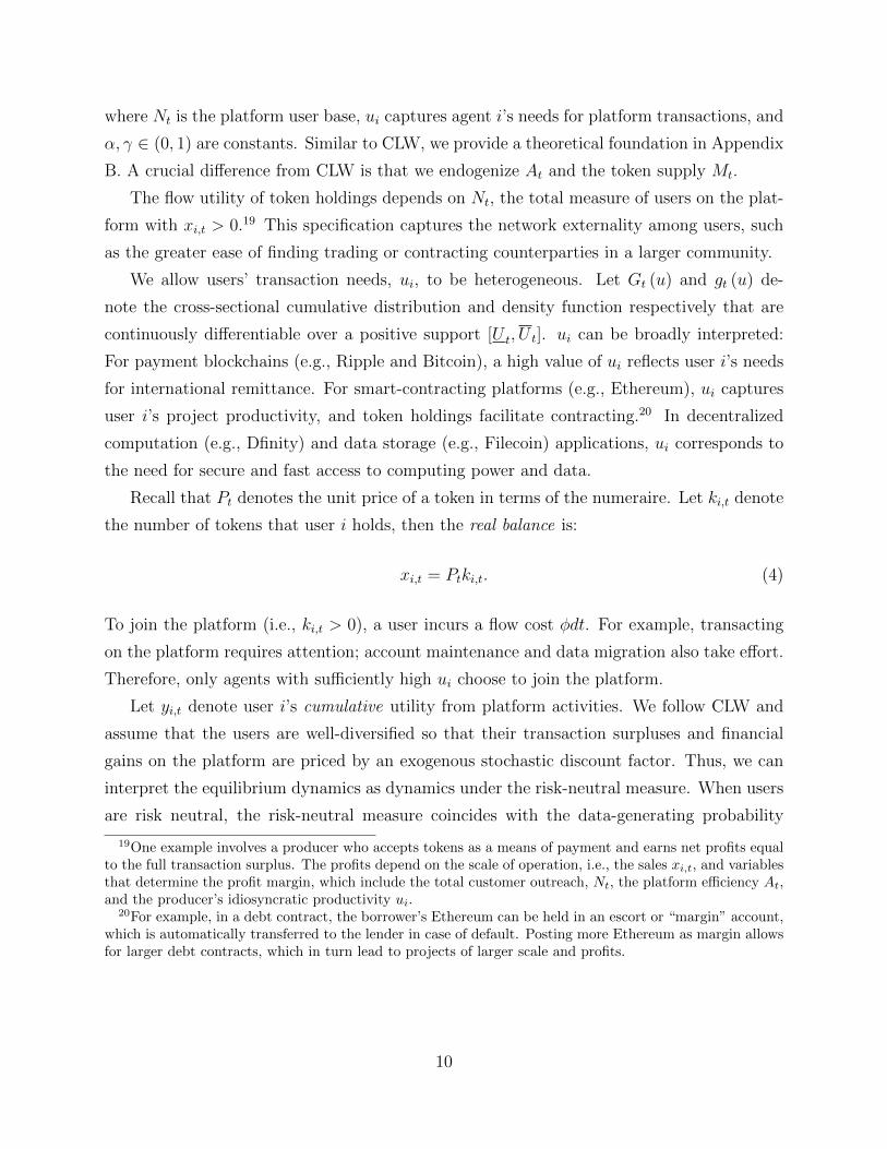
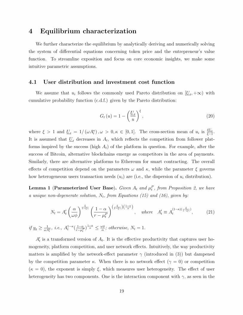
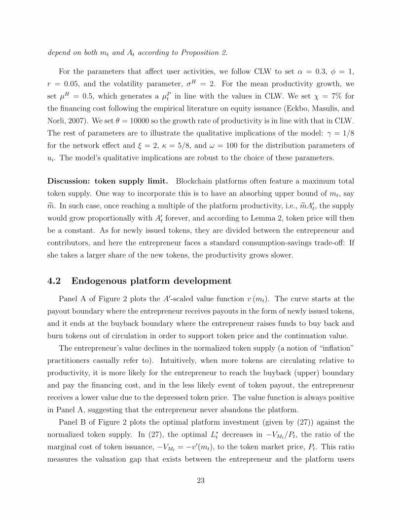
Panel A of Figure 2 plots the A′-scaled value function v (mt). The curve starts at the

payout boundary where the entrepreneur receives payouts in the form of newly issued tokens,

and it ends at the buyback boundary where the entrepreneur raises funds to buy back and

burn tokens out of circulation in order to support token price and the continuation value.

The entrepreneur’s value declines in the normalized token supply (a notion of “inflation”

practitioners casually refer to). Intuitively, when more tokens are circulating relative to

productivity, it is more likely for the entrepreneur to reach the buyback (upper) boundary

and pay the financing cost, and in the less likely event of token payout, the entrepreneur

receives a lower value due to the depressed token price. The value function is always positive

in Panel A, suggesting that the entrepreneur never abandons the platform.

Panel B of Figure 2 plots the optimal platform investment (given by (27)) against the

normalized token supply. In (27), the optimal L∗t decreases in −VMt/Pt, the ratio of the

marginal cost of token issuance, −VMt = −v′(mt), to the token market price, Pt. This ratio

measures the valuation gap that exists between the entrepreneur and the platform users

23

11

1 1

Figure 2: Platform Value and Investment. Panel A plots the A′t-scaled value function. Panel B plotsthe optimal investment as a function of productivity-normalized token supply, mt. Panel C shows the ratioof the entrepreneur’s marginal value of tokens to the market price of tokens, and the wedge between thisratio and one represents the token issuance cost. Panel D shows the entrepreneur’s marginal value of A′t.

(i.e., the token issuance cost). When the gap is high, it is costly from the entrepreneur’s

perspective to finance investment with tokens. The ratio starts at one, as implied by the

value-matching condition of the payout boundary. This is when the entrepreneur’s private

valuation of tokens, which incorporates the expected cost of token buyback, coincides with

the market or users’ valuation. The gap widens as the token supply outpaces the growth of

the effective productivity, i.e., as mt increases, and eventually, when the gap reaches (1 + χ),

the entrepreneur optimally buys back tokens. The increasing token issuance cost in Panel C

(i.e., −VMt/Pt increasing in mt) largely contributes to the decreasing pattern of L∗t .

The optimal L∗t given by (27) increases in the marginal value of effective productivity,∂Vt∂A′t

= v(mt)−v′(mt)mt, because on average, investment has a positive outcome, i.e., µH > 0,

so more resources gathered by token payments, Lt, leads to a higher expected growth of

At and an expected increase in the entrepreneur’s value. Moreover, the marginal value of

effective productivity also has a positive impact on L∗t via the denominator of L∗t in (27).

As shown in the HJB equation (26), the marginal value of A′t is multiplied by the drift of

A′ (= Aδt ), which is equal to δµHLt + 12δ(δ − 1)(σH)2L2

t given dAt in (2). The denominator

effect follows the quadratic term in the drift of A′t. Near the buyback (upper) boundary, ∂Vt∂A′t

24

is particularly high because an increase in A′t pulls down mt and thus reduces the likelihood

of costly buyback. Overall, even though the marginal value of productivity is increasing in

mt in Panel D, the economic force of token overhang (Panel C) dominates, resulting in an

optimal investment that declines in the normalized token supply mt.

Finally, according to (27), the second-order derivative of the A′-scaled value function,

v′′(mt), also affects the optimal investment L∗t via the denominator. Its impact is small

under the current parameterization, so the plot is omitted from Figure 2. However, the

intuition of the potential precautionary motive (v′′(mt) < 0) is still interesting. Token

payout is largely a real option decision. While it is not completely irreversible, reversing it

(i.e., buying back tokens) incurs the financing cost.27 The probability of incurring such cost

increases as mt approaches the buyback boundary, so the entrepreneur becomes increasingly

cautious on making a risky investment given the shock in (2). Therefore, the negative impact

of precaution on investment is more prominent near the buyback (upper) boundary of mt.

Overall, our model reveals a rich set of trade-offs in the choice of token-financed in-

vestment. The model has the potential to explain various features of token distribution to

open-source engineers, miners (ledger maintainers), and crowd-sourced financiers in practice.

4.3 Token price and user adoption

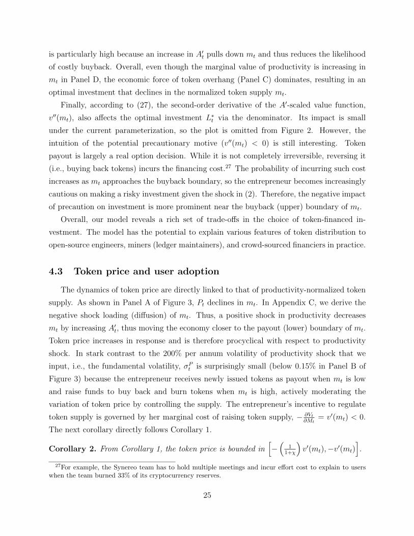
The dynamics of token price are directly linked to that of productivity-normalized token

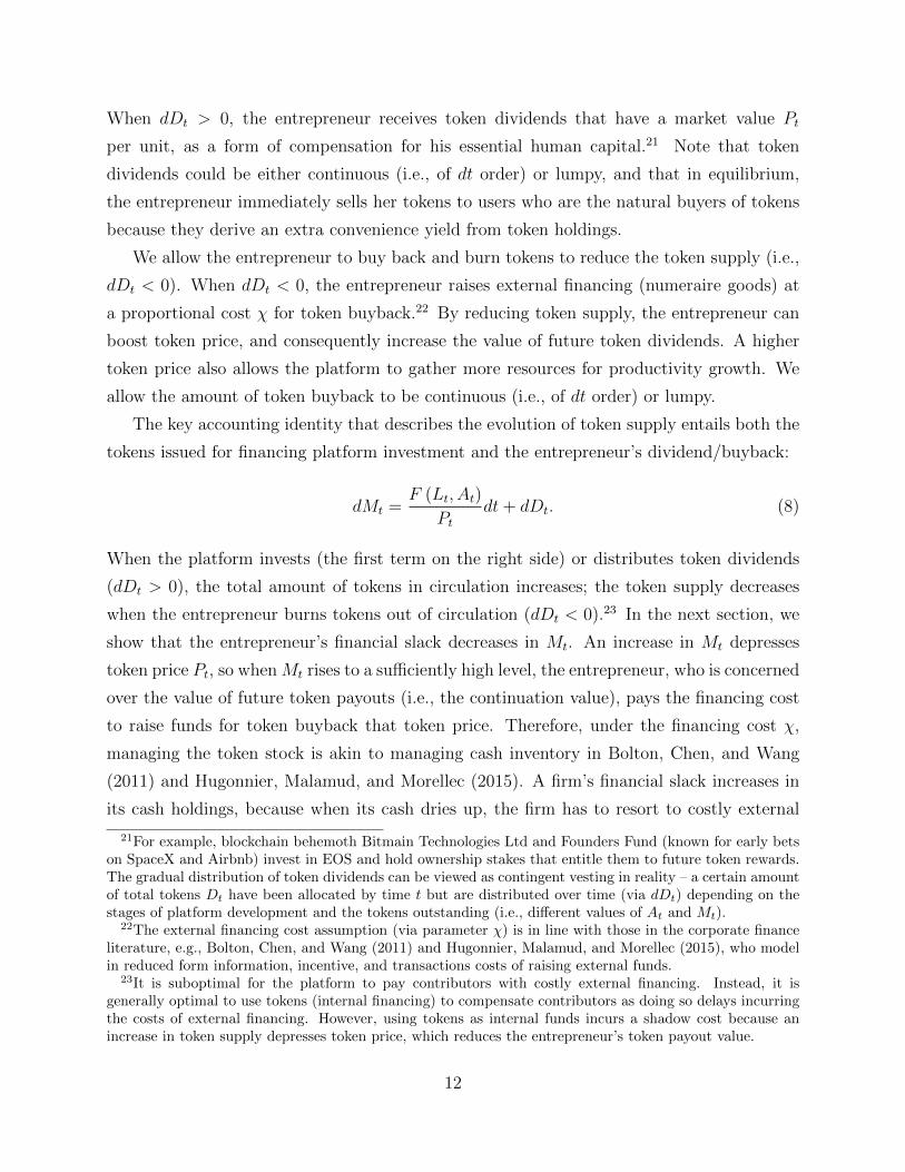
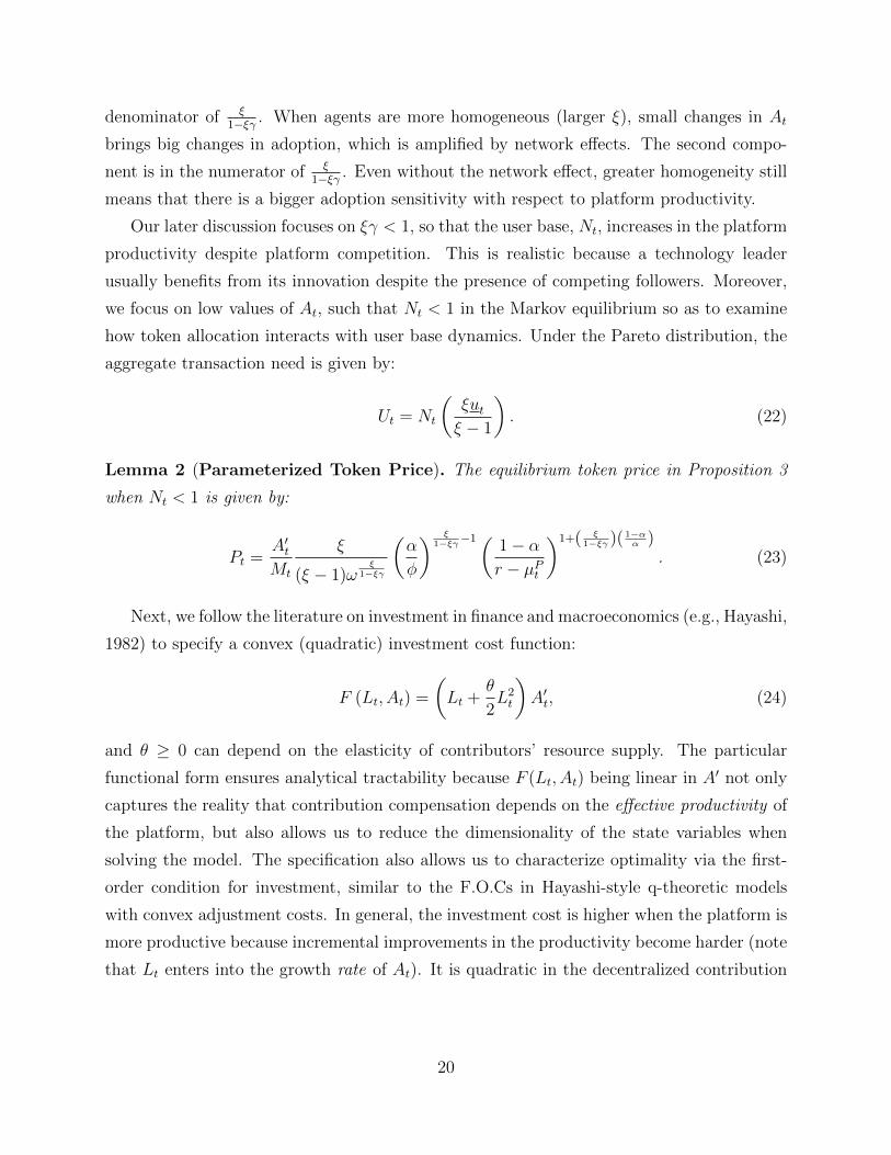
supply. As shown in Panel A of Figure 3, Pt declines in mt. In Appendix C, we derive the

negative shock loading (diffusion) of mt. Thus, a positive shock in productivity decreases

mt by increasing A′t, thus moving the economy closer to the payout (lower) boundary of mt.

Token price increases in response and is therefore procyclical with respect to productivity

shock. In stark contrast to the 200% per annum volatility of productivity shock that we

input, i.e., the fundamental volatility, σPt is surprisingly small (below 0.15% in Panel B of

Figure 3) because the entrepreneur receives newly issued tokens as payout when mt is low

and raise funds to buy back and burn tokens when mt is high, actively moderating the

variation of token price by controlling the supply. The entrepreneur’s incentive to regulate

token supply is governed by her marginal cost of raising token supply, − ∂Vt∂Mt

= v′(mt) < 0.

The next corollary directly follows Corollary 1.

Corollary 2. From Corollary 1, the token price is bounded in[−(

11+χ

)v′(mt),−v′(mt)

].

27For example, the Synereo team has to hold multiple meetings and incur effort cost to explain to userswhen the team burned 33% of its cryptocurrency reserves.

25

'''

11

1 1

Figure 3: Token Price Dynamics and User Adoption. Panel A plots token price against productivity-normalized token supply, mt. Panel B plots σP

t , the Pt-scaled diffusion term of token price. Panel C showsthe Pt-scaled drift of token price. Panel D plots the user base, which depends on both mt and A′t.

The optimality condition on payout imposes an upper bound on token price. At any

mt, P (mt) ≤ −v′(mt) because otherwise the entrepreneur prefers obtaining token payout

(worth P (mt) per unit of token) over preserving the continuation value (worth −v′(mt)).

The optimality condition on token buyback imposes a lower bound on token price. At any

mt, P (mt) ≥ −(

11+χ

)v′(mt) because otherwise the entrepreneur finds tokens too cheap in

the secondary market and prefers raising costly funds to buy back tokens. In our model, the

token value has two anchors. First, users need tokens for transactions. Second, to preserve

the continuation value, the entrepreneur is willing to pay the financing cost to raise funds

and use such real resources to buy back and burn tokens out of circulation.

Panel C of Figure 3 shows the expected token price change. When mt is low, the ex-

pectation is negative, reflecting the likely token-supply increase due to token payout to the

entrepreneur and increasing investment needs (Panel A of Figure 2). As mt increases, the

expected change in token price gradually increases and eventually becomes positive because,

first, the investment needs decline, and second, the likelihood of token buyback increases.

26

Finally, we report the results on user-base dynamics. As shown in Proposition 2, unlike

other endogenous variables that only depends on mt, the user base Nt depends on both mt

(through the expected token price change µP (mt)) and A′t. Panel D of Figure 3 plots the user

base against mt under different values of A′t. Given A′t, Panel D shows that as mt increases

(and µPt increases), the user base increases because agents expect an improving capital gain

from token holdings. Given any value mt, a higher value of productivity At leads to a larger

user base because At directly enters users’ convenience yield from token holdings in (3).

Discussion: Stablecoins. Our model features mild volatility of token price. The en-

trepreneur’s optimal payout and token buyback decisions impose two reflecting boundaries

on the state variable mt. At both boundaries, the first derivative of token price with respect

to mt must be zero (e.g., see (30)) because otherwise arbitrage opportunities emerge: For

example, at m, mt will be reflected upward for sure, so P ′(mt) > 0 (< 0) implies guaranteed

instantaneous profits from a long (short) position. By Ito’s lemma, P ′(mt) = 0 at the bound-

aries implies σP (mt) = 0. Therefore, even in the interior region, token volatility σP (mt) can

exceed zero; however, it cannot go far beyond zero as it is tied to zero at both boundaries.

Therefore, in our model, the stability of token price relies on the dynamic payout and

token buyback decisions of the entrepreneur. This mechanism differs significantly from the

stablecoin designs proposed by practitioners. A popular approach is to mimic open market

operations by central banks. When token price is low, the platform issues token bonds to

buy back tokens. Token bonds promise to pay the principal with interest in the future,

but all payments are in tokens. The problem with this design is that an inter-temporal

substitution between current and future tokens does not introduce any real resources to

support token price, nor does it provide any incentive to economic agents to devote such

resources. A champion of this design, the Basis stablecoin project, which attracted $133

million of venture capital in April 2017, has closed down all operations, citing US securities

regulations as the reason for its decision.28 An alternative design is collateralization, which

backs token value with real resources, such as the U.S. dollar (e.g., Tether, Circle, Gemini,

JPM coin, or Paxos), oil reserves (e.g., Venezuela’s El Petro, OilCoin, or PetroDollars).29

A derivative of such design is to further tranche the claims on real resources, so tokens are

the most senior tranche, which is less information-sensitive and thus has a stable secondary-

28https://icoexaminer.com/ico-news/133-million-basis-stablecoin-project-ceases-and-desists-citing-regulatory-concerns/

29Such designs are often subject to manipulations (e.g., Griffin and Shams, 2018).

27

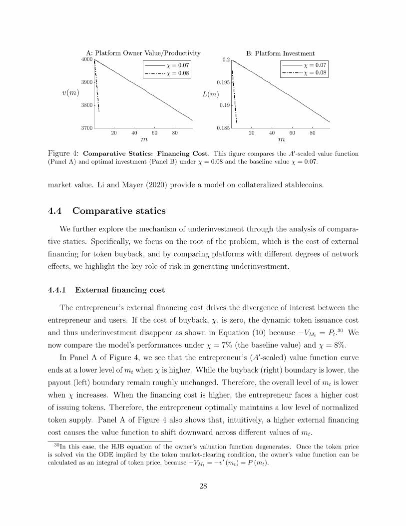
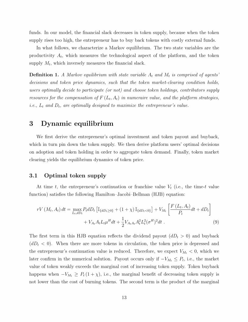
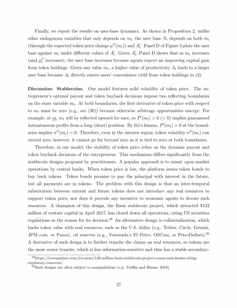
Figure 4: Comparative Statics: Financing Cost. This figure compares the A′-scaled value function(Panel A) and optimal investment (Panel B) under χ = 0.08 and the baseline value χ = 0.07.

market value. Li and Mayer (2020) provide a model on collateralized stablecoins.

4.4 Comparative statics

We further explore the mechanism of underinvestment through the analysis of compara-

tive statics. Specifically, we focus on the root of the problem, which is the cost of external

financing for token buyback, and by comparing platforms with different degrees of network

effects, we highlight the key role of risk in generating underinvestment.

4.4.1 External financing cost

The entrepreneur’s external financing cost drives the divergence of interest between the

entrepreneur and users. If the cost of buyback, χ, is zero, the dynamic token issuance cost

and thus underinvestment disappear as shown in Equation (10) because −VMt = Pt.30 We

now compare the model’s performances under χ = 7% (the baseline value) and χ = 8%.

In Panel A of Figure 4, we see that the entrepreneur’s (A′-scaled) value function curve

ends at a lower level of mt when χ is higher. While the buyback (right) boundary is lower, the

payout (left) boundary remain roughly unchanged. Therefore, the overall level of mt is lower

when χ increases. When the financing cost is higher, the entrepreneur faces a higher cost

of issuing tokens. Therefore, the entrepreneur optimally maintains a low level of normalized

token supply. Panel A of Figure 4 also shows that, intuitively, a higher external financing

cost causes the value function to shift downward across different values of mt.

30In this case, the HJB equation of the owner’s valuation function degenerates. Once the token priceis solved via the ODE implied by the token market-clearing condition, the owner’s value function can becalculated as an integral of token price, because −VMt = −v′ (mt) = P (mt).

28

Figure 5: Comparative Statics: Network Effect. This figure compares the A′-scaled value function(Panel A) and optimal investment (Panel B) under γ = 0.124 and the baseline value γ = 0.125.

We compare platform investment under different values of χ in Panel B of Figure 4.

A higher financing cost leads to lower investment as the conflict of interest between the

entrepreneur and users is exacerbated. Following a positive shock, the investment success-

fully enhances productivity, benefiting both the entrepreneur and users; following a negative

shock, only the entrepreneur bears the downside of a higher likelihood of paying the financ-

ing cost for token buyback because users are free to reduce token holdings and abandon the

platform. A higher financing cost implies a greater downside for the entrepreneur.

4.4.2 Network effect

As specified in (3), the parameter γ governs the strength of the network effect. When

γ is higher, an increase in the total number of users, Nt, causes each user to demand more

tokens. In Figure 5, we compare the entrepreneur’s value function (Panel A) and optimal

investment (Panel B) under γ = 0.125 (the baseline value) and γ = 0.124.

Interestingly, a weaker network effect induces the entrepreneur to be more aggressive in

token issuance. Moreover, the entrepreneur’s value function shifts upward (Panel A), as a

weaker network effect induces more investment (Panel B). These observations are counterin-

tuitive because when the network effect is weaker, the positive feedback effect of increasing

productivity to attract more and more users is dampened, which discourages investment in

productivity. However, our model features a counteracting force.

As previously discussed, the conflict of interest between the entrepreneur and users and

the resultant underinvestment problem depend on three ingredients: (1) the external financ-

ing cost, (2) user heterogeneity, and (3) the uncertainty in investment outcome. When in-

vestment outcome is uncertain, the entrepreneur has to consider the potential downside, i.e.,

29

the increase in the likelihood of costly token buyback follows a negative shock that increases

mt (by decreasing productivity in the denominator). A weaker network effect dampens un-

certainty. Following a positive shock, investment increases productivity, but under a weaker

network effect, the resultant increase in token demand and price is smaller. Likewise, follow-

ing a negative shock, a weaker network effect implies a smaller decline in token demand and

price. Therefore, even though a weaker network effect reduces the average positive impact of

investment on token price and the entrepreneur’s payout (the mean effect), it also dampens

the risk of investment, which is a key ingredient of the underinvestment problem.

5 Blockchain and investment efficiency

The entrepreneur faces a time inconsistency problem that features prominently in stud-

ies on macroeconomics (Kydland and Prescott, 1980; Barro and Gordon, 1983; Lucas and

Stokey, 1983) and corporate capital structure (DeMarzo and He, 2020). If the entrepreneur

is able to commit against underinvestment, the users would have demanded more tokens,

which then increases token price, as well as the value of token payouts to the entrepreneur.

However, a predetermined level of investment can be deemed suboptimal ex post as the

conflict of interest arises between the entrepreneur and users, reflected in the gap between

the entrepreneur’s private valuation of tokens, −VMt , and users’ valuation, Pt.

So far, we have focused on the discretionary token-supply policies of the platform. Next,

we study how commitment to predetermined token-supply rules adds value. Our analysis

sheds light on why tokens become a viable payment solution after the blockchain technology

matures. The rise of tokens as a means of payment on digital platforms is a recent phe-

nomenon with many applications inspired by the success of Bitcoin, Ethereum, and other

blockchain-based startups. In Appendix A, we summarize the three aspects of blockchain

technology that are critical in enabling commitment, including data structure, smart con-

tracting, decentralized governance, and we highlight both the advantages of blockchain-based

commitment over traditional approaches (e.g., collateral) and its limitations.

30

5.1 Constant token growth as commitment to investment

To illustrate the impact of commitment brought forth by the blockchain technology, we

consider a specific case where:

dMt = F (Lt, At) /Ptdt = µMMtdt, (34)

i.e., a constant growth rate of token supply in the interior region (dDt = 0) to finance

the enhancement of platform productivity. This commitment is popular among blockchain

applications primarily as a way to address users’ concern over token-holding dilution via

inflation.31 We show that the fundamental role of such commitment actually lies in the mit-

igation of underinvestment. This rule of token supply implies that the resources a platform

gathers, Lt, become a predetermined function of the state variables.

We still allow the entrepreneur to receive token dividends and buy back tokens, but

with Lt following a predetermined rule, the entrepreneur’s only control variable is dDt. The

following HJB equation characterizes the value function:

rV (Mt, At) dt = maxdDt

PtdDt

[I{dDt≥0} + (1 + χ) I{dDt<0}

]+ VMt

(µMMtdt+ dDt

)+ VAtAtLtµ

Hdt+1

2VAtAtA

2tL

2t (σ

H)2dt. (35)

Comparing it with Equation (9), the tokens used to pay for Lt is replaced by µMMtdt. Under

the same change of variable as in Section 4.1, we have, in the interior region (dDt = 0)

rv (mt) =v′ (mt)

(Lt + θ

2L2t

)P (mt)

+ [v (mt)− v′ (mt)mt]

[δµHLt +

1

2δ(δ − 1)(σH)2L2

t

]+

1

2v′′ (mt)m

2t δ

2(σH)2L2t , (36)

where Lt, as a function of mt, is implicitly defined by:

Lt +θ

2L2t = µMP (mt)mt . (37)

As the left side of (37) is an increasing and convex function of Lt, investment increases in the

A′-scaled token market capitalization, i.e., P (m)m = PtMt/A′t. Intuitively, when tokens are

31Blockchain applications emphasize predetermined rules of token-supply growth. Ethereum has roughlyfixed increments while Bitcoin’s minting rate is a constant that halves as the system matures via a longertransaction chain (specifically, every 210,000 more blocks).

31

C D

µM = 1 µM = 1

µM = 2 µM = 2

Figure 6: Platform Value and Investment under Predetermined Token-Supply Growth. PanelsA and C plot, respectively, the A′t-scaled value functions under µM = 2 and µ=1. Panel B and D plot,respectively, the optimal investment under µM = 2 and µM = 1.

more valuable, the constant growth of token supply gathers more resources for development.

The boundary conditions are the same as those of the baseline model.

Proposition 5 (Solution under Predetermined Token Growth). Under the commit-

ment to a constant growth rate of token supply for investment in productivity, the investment

given by Equation (37) increases in A′-scaled token market capitalization, i.e., Ptmt. The

entrepreneur receives token dividends (dD∗t > 0) when Pt ≥ −VMt, and buys back and burns

tokens out of circulation (dD∗t < 0) when −VMt ≥ Pt (1 + χ). Token price is determined by

Equation (23) as in the baseline model.

In our numerical solution, we start with µM = 2 for illustrative purpose. Comparing

Panel A of Figure 6 with Panel A of Figure 2, we can see that the commitment increases the

entrepreneur’s value by around 15% near the payout (lower) boundary and around 20% near

the buyback (upper) boundary. By comparing Panel B in the two figures, we see that such

an increase mainly comes from a higher level of investment as the commitment mitigates the

problem of underinvestment under token overhang.

32

As previously discussed, to the entrepreneur, the value of tokens is −VMt , while to the

users, it is Pt. The wedge between −VMt and Pt widens as the normalized token supply,

mt, increases, and the ratio, −VMt/Pt, reaches 1 + χ, the financing cost of token buyback,

at the buyback (upper) boundary of mt. Therefore, as shown in (10), the closer to the

buyback boundary, the more concerned the entrepreneur is over the token issuance cost,

−VMt/Pt > 1. This implies that investment chosen by the entrepreneur declines in mt as

shown in Panel B of Figure 2. Therefore, commitment to the predetermined investment rule

creates more value when mt is higher and closer to its upper boundary. This explains why the

commitment-induced improvement in the entrepreneur’s value is greater near the buyback

boundary (around 20% increase) than near the payout boundary (around 15% increase).

Another difference between the commitment case and the baseline case of discretionary

investment is that under commitment, investment increases in mt (Panel B of Figure 6),

while in the baseline case, investment decreases in mt (Panel B of Figure 2). As previously

discussed, the declining pattern in the baseline case is due to the increasing cost of issuing

tokens, i.e., the widening wedge between −VMt and Pt. The increasing pattern in the com-

mitment case is a numeric result. As mt increases, token price, P (mt), decreases, but the

A′t-scaled market capitalization, i.e., P (mt)mt, may increase or decrease. Under the current

parameterization, the P (mt)mt increases in mt, so, according to (37), Lt increases in mt.

To further demonstrate the economic mechanism, we also consider the solution when the

committed growth of token supply is half as large, i.e., µM = 1. The impact of reducing

token-supply growth rate on investment and the entrepreneur’s value is unclear a priori. By

reducing inflation, a lower growth rate of token supply tends to increase the token price

that users are willing to pay and thus increase Lt, the resources gathered via token issuance.

However, as shown in (37), Lt depends on the token market capitalization, i.e., both the unit

price and the quantity of tokens, so reducing the token-supply growth can also negatively

impact Lt. Under the current parameterization, the latter force dominates, which leads to

a lower level of investment under µM = 1 (Panel D of Figure 6) than the solution under

µM = 2 (Panel B of Figure 6). Comparing Panels A and C of Figure 6, we can see that the

entrepreneur’s value also declines when µM declines from 2 to 1.

What is more interesting is that the entrepreneur’s value near the payout (lower) bound-

ary of mt is not only below the value under µM = 2 but also around 2% below the value in

the baseline case of discretionary investment (Panel A of Figure 2). As previously discussed,

the wedge between the entrepreneur’s private cost of token issuance, −VMt , and users’ valua-

tion, Pt, widens as mt increases, so commitment adds more value when mt is higher. Indeed,

33

the entrepreneur’s value is around 3% higher under µM = 1 than in the discretionary case

near the buyback (upper) boundary. In contrast, commitment adds less value in the low-mt

region, i.e., near the payout (lower) boundary, because the conflict of interest between the

entrepreneur and users is less severe. Therefore, near m, the value added from commitment

is small while the drawback of commitment—the entrepreneur cannot coordinate investment

(Lt) and payout/buyback (dDt) decisions—dominates. As a result, the entrepreneur’s value

actually decreases under commitment relative to the discretionary case.

Regarding the coordination between investment and payout/buyback decisions, its im-

portance can be seen from the difference in the range of mt on the horizontal axis between

commitment cases (Figure 6) and the baseline case (Figures 2 and 3). Under commitment,

the range is much smaller. The entrepreneur pays the financing cost to buy back and burn

tokens at a much lower level of mt (i.e., chooses a lower buyback boundary). Moreover, the

payout boundaries under commitment (both µM = 1 and µM = 2) are higher than that of the

discretionary case. Therefore, when the entrepreneur loses control of the amount of tokens

issued for investment, she turns more active in payout and buyback, effectively narrowing

the equilibrium range of mt. This results in more frequency payments of the financing cost.

To sum up, commitment to predetermined investment rules adds value by addressing

the token overhang problem, but it also forces the entrepreneur to control the token supply

more actively via the remaining margins (i.e., payout and buyback), and to pay the financing

cost more frequently. Overall, when the former force dominates, the entrepreneur obtains

a higher value via commitment: A higher level of investment translates into a higher token

price through users’ expectation of faster productivity growth, and a higher token price in

turn implies more valuable token payout for the entrepreneur.

5.2 Mitigating underinvestment through fees

As demonstrated, commitment enabled by blockchains alleviates the problem of token-

overhang and underinvestment, but commitment to predetermined investment rules forces

the entrepreneur to manage the token supply through more active payout and buyback,

which results in paying the financing cost more frequently. An alternative solution is to

finance investment with fees collected from users.

To analyze the impact of fees, let f0,t and f1,t denote respectively the fixed and propor-

34

tional fees users pay at t. The users’ objective (6) is modified to:

max

{0, max

ki,t>0

[(Ptki,t)

1−α (Nγt Atui)

α dt+ ki,tEt [dPt]− (φ+ ft,0)dt− Ptki,t(r + f1,t)dt]}

.

(38)

Under the parameterized distribution of ui, we follow the same procedure to solve the par-

ticipation threshold and then obtain a new measure of users:

Nt = A′t

(α

ω(φ+ f0,t)

) ξ1−ξγ

(1− α

r + f1,t − µP (mt)

)( ξ1−ξγ )( 1−α

α )≡ A′tn(f0,t, f1,t,mt) . (39)

It is clear that ∂n(f0,t,f1,t,mt)

∂f0,t< 0 and ∂n(f0,t,f1,t,mt)

∂f1,t< 0 (as α ∈ (0, 1) and ξ ∈ (1, 1/γ]). The

platform faces a trade-off. Higher fees, either via f0,t or f1,t, lead to lower user participation,

which directly reduces the revenue from fixed fees, i.e., f0,tNt.32

Meanwhile, higher fees also reduce users’ token demand, which leads to a lower token

price and proportional fees. We follow the same procedure of solving users’ token demand,

ki,t, and then from the token market-clearing condition, we obtain:

P (f0,t, f1,t,mt) =ξ

mt(ξ − 1)ωξ

1−ξγ

(α

φ+ f0,t

) ξ1−ξγ−1

(1− α

r + f1,t − µP (mt)

)1+( ξ1−ξγ )( 1−α

α ).

(40)

We have ∂P (f0,t,f1,t,mt)

∂f0,t< 0 and ∂P (f0,t,f1,t,mt)

∂f1,t< 0 (as ξ

1−ξγ − 1 > 0 under ξγ < 1), so token

price is negatively affected by the platform imposing fees on users.

Overall, when choosing fees, the entrepreneur solves a problem akin to a monopolistic

producer, trading off unit prices and quantities. The total fee revenues are equal to f0,tNt +

f1,tPtMt, where we apply the token market-clearing condition,∫i∈[0, 1] ki,tdi = Mt to substitute

out ki,t. Such revenues can be used to finance investment in productivity so that the need

to issue tokens is reduced. The new law of motion of token supply is thus given by:

dMt =F (Lt, At)− (f0,tNt + f1,tPtMt)

Ptdt+ dDt , (41)

32Note that the users’ expectation of the rate of token price change, µP (mt), is a function of the key statevariable mt, which the platform takes as given when choosing its fees.

35

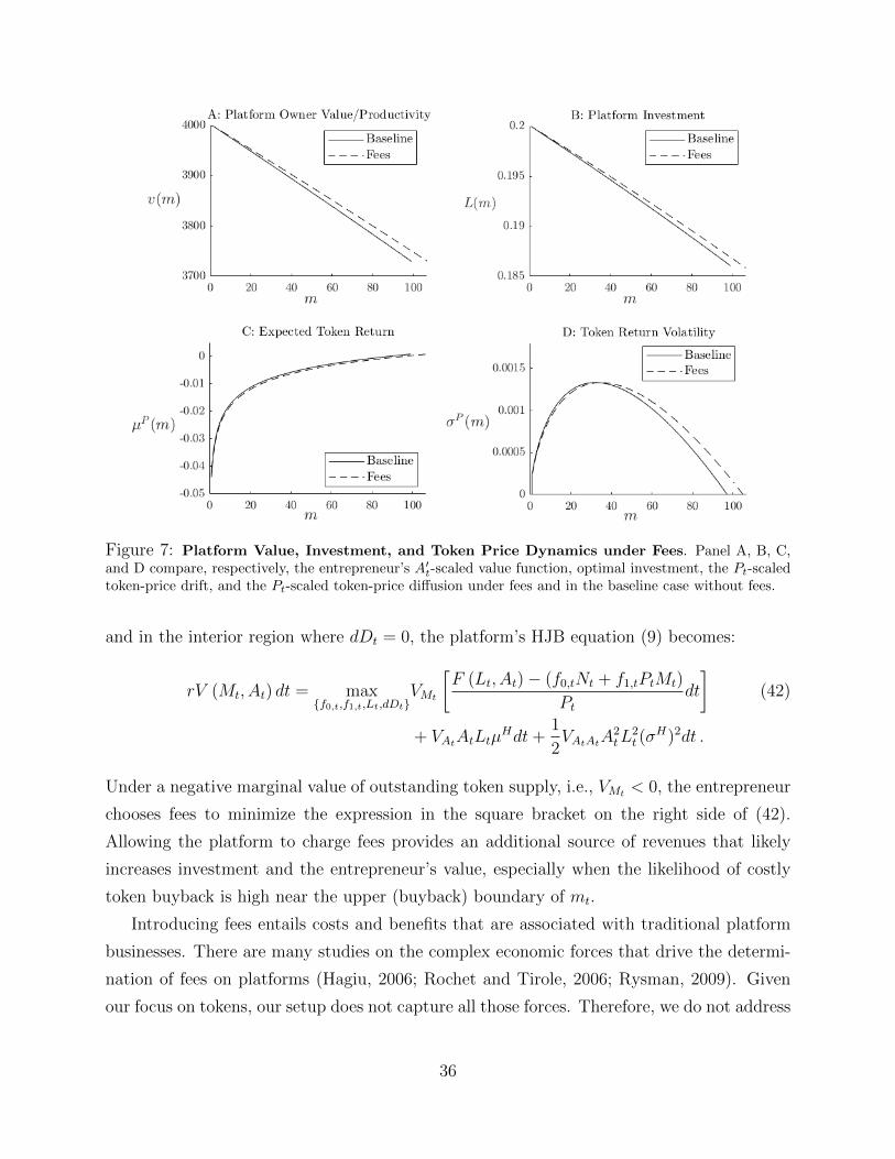
Figure 7: Platform Value, Investment, and Token Price Dynamics under Fees. Panel A, B, C,and D compare, respectively, the entrepreneur’s A′t-scaled value function, optimal investment, the Pt-scaledtoken-price drift, and the Pt-scaled token-price diffusion under fees and in the baseline case without fees.

and in the interior region where dDt = 0, the platform’s HJB equation (9) becomes:

rV (Mt, At) dt = max{f0,t,f1,t,Lt,dDt}

VMt

[F (Lt, At)− (f0,tNt + f1,tPtMt)

Ptdt

](42)

+ VAtAtLtµHdt+

1

2VAtAtA

2tL

2t (σ

H)2dt .

Under a negative marginal value of outstanding token supply, i.e., VMt < 0, the entrepreneur

chooses fees to minimize the expression in the square bracket on the right side of (42).

Allowing the platform to charge fees provides an additional source of revenues that likely

increases investment and the entrepreneur’s value, especially when the likelihood of costly

token buyback is high near the upper (buyback) boundary of mt.

Introducing fees entails costs and benefits that are associated with traditional platform

businesses. There are many studies on the complex economic forces that drive the determi-

nation of fees on platforms (Hagiu, 2006; Rochet and Tirole, 2006; Rysman, 2009). Given

our focus on tokens, our setup does not capture all those forces. Therefore, we do not address

36

the question of optimal fee setting. Instead, we illustrate the impact of fees in Figure 7 using

a particular fee structure f0,t = 0.1% and f1,t = 0.1%.33 The fee revenue, f0,tNt + f1,tPtMt,

varies endogenously in the model, along with the user base, Nt, the token price, Pt, and the

outstanding token amount, Mt. The constant fee parameters allow us to remain as close as

possible to the baseline model and its solution method.

The dashed line in Panel A of Figure 7 shows that fees increase the platform owner’s

value especially near the buyback (upper) boundary of mt. As previously discussed, near

the upper boundary, the token issuance cost is high, so the platform refrains from token-

financed investment. This underinvestment problem is now mitigated by fee revenues (Panel

B of Figure 7). Introducing fees does not significantly affect the dynamics of token price

(Panels C and D of Figure 7) in terms of the drift and diffusion. A notable difference between

our main model and the model with fees is that under fees, the entrepreneur delays costly

token buyback, which is reflected in a higher upper boundary of mt (Panel D of Figure 7).

This additional financial slack also helps to boost the entrepreneur’s value.

Overall, fees increase the entrepreneur’s value by both alleviating the underinvestment

problem and allowing the platform to reduce the impact of financing costs by postponing

token buybacks. Our analysis thus points towards an interesting direction for future research:

Analogous to macroeconomic management through monetary and fiscal policies, a platform

may dynamically manage its state-contingent token-supply policy and fee structure.

6 Conclusion

We develop a dynamic model of a platform economy, where tokens are used as a means

of payment among users and issued to finance platform operation and growth. Tokens facil-

itate user transactions and compensate distributed ledger-keepers, open-source developers,

and crowdfunders for their contributions to platform development. The platform owners

maximize their seigniorage by managing token supply, subject to the conditions that users

optimally decide on token demand and rationally form expectation of token price dynamics.

We characterize the optimal token-supply strategy and its implications for user-base

dynamics, endogenous platform growth, and token price dynamics. A key mechanism is

33When fees are set by centralized platform owners, they are relatively stable, as we see in IBM Blockchain’sflat fee for IBM Cloud, for example (https://cloud.ibm.com/docs/blockchain?topic=blockchain-ibp-saas-pricing). Fee setting on permissionless, decentralized platforms has traditionally been linked to networkcongestion and service capacity, which are outside our model but discussed in Cong, Li, and Wang (2018)and Basu, Easley, O’Hara, and Sirer (2019).

37

the wedge between insiders’ (the platform owners’) token valuation and that of outsiders

(users). When the valuation wedge falls to zero, the platform owners optimally receives token

dividends; when it rises to an endogenously determined threshold, the platform optimally

burns tokens out of circulation to stabilize token value. The wedge creates underinvestment

in platform productivity under the financing cost of token buyback.

By enabling commitment, blockchains enable rule-based token supply, thereby mitigating

underinvestment by overcoming the platform owners’ time inconsistency. Financing invest-

ment with fees charged on users reduces the investment inefficiency at the expense of user

participation and token demand. Beyond the main focus on token-financed platform devel-

opment, our paper provides broad implications of dynamic token allocation for token price,

user adoption, stablecoins, among other issues.

38

References

Abadi, Joseph, and Markus Brunnermeier, 2018, Blockchain economics, Discussion paper, mimeoPrinceton University.

Barro, Robert J., and David B. Gordon, 1983, A positive theory of monetary policy in a naturalrate model, Journal of Political Economy 91, 589–610.

Basu, Soumya, David Easley, Maureen O’Hara, and Emin Sirer, 2019, Towards a functional feemarket for cryptocurrencies, Available at SSRN 3318327.

Biais, Bruno, Christophe Bisiere, Matthieu Bouvard, and Catherine Casamatta, 2019, Theblockchain folk theorem, The Review of Financial Studies 32, 1662–1715.

Bolton, Patrick, Hui Chen, and Neng Wang, 2011, A unified theory of tobin’s q, corporate invest-ment, financing, and risk management, The Journal of Finance 66, 1545–1578.

Bolton, Patrick, and Haizhou Huang, 2017, The capital structure of nations, Review of Finance 22,45–82.

Brunnermeier, Markus K., Harold James, and Jean-Pierre Landau, 2019, The digitalization ofmoney, Discussion paper, Princeton University.

Brunnermeier, Markus K., and Yuliy Sannikov, 2016, The I theory of money, Working paperPrinceton University.

Bulow, Jeremy I, 1982, Durable-goods monopolists, Journal of political Economy 90, 314–332.

Cagan, Phillip D., 1956, . The monetary dynamics of hyperinflation, (University of Chicago Press).

Canidio, Andrea, 2018, Financial incentives for open source development: the case of blockchain,working paper IMT School of Advanced Studies.

Chiu, Jonathan, and Thorsten V Koeppl, 2017, The economics of cryptocurrencies–Bitcoin andbeyond, Working Paper.

Chiu, Jonathan, and Tsz-Nga Wong, 2015, On the essentiality of e-money, Discussion paper, Bankof Canada Staff Working Paper.

Chod, Jiri, and Evgeny Lyandres, 2018, A theory of ICOs: Diversification, agency, and asymmetricinformation, Working paper Boston University Questrom School of Business.

Coase, R. H., 1972, Durability and monopoly, The Journal of Law and Economics 15, 143–149.

Cong, Lin William, and Zhiguo He, 2019, Blockchain disruption and smart contracts, The Reviewof Financial Studies 32, 1754–1797.

Cong, Lin William, Ye Li, and Neng Wang, 2018, Token-based corporate finance, Working Paper.

, 2020, Tokenomics: Dynamic adoption and valuation, Review of Financial Studies forth-coming.

Decamps, Jean-Paul, Sebastian Gryglewicz, Erwan Morellec, and Stphane Villeneuve, 2016, Cor-porate Policies with Permanent and Transitory Shocks, The Review of Financial Studies 30,162–210.

39

DeMarzo, Peter M., and Zhiguo He, 2020, Leverage dynamics without commitment, The Journalof Finance forthcoming.

Duffie, Darrell, 2019, Digital currencies and fast payment systems: Disruption is coming, workingpaper Stanford University Graduate School of Business.

Easley, David, Maureen O’Hara, and Soumya Basu, 2019, From mining to markets: The evolutionof bitcoin transaction fees, Journal of Financial Economics 134, 91–109.

Eckbo, B. Espen, Ronald W. Masulis, and Oyvind Norli, 2007, Chapter 6 – security offerings, inB. Espen Eckbo, ed.: Handbook of Corporate Finance: Empirical Corporate Financevol. 1 ofHandbook of Finance Series . pp. 233–373 (Elsevier/North-Holland).

Fanti, Giulia, Leonid Kogan, and Pramod Viswanath, 2019, Economics of proof-of-stake paymentsystems, Working paper.

Fischer, Stanley, 1980, Dynamic inconsistency, cooperation and the benevolent dissembling govern-ment, Journal of Economic Dynamics and Control 2, 93–107.

Garratt, Rodney, and Maarten R.C. Van Oordt, 2019, Entrepreneurial incentives and the roleof initial coin offerings, working paper University of California at Santa Barbara and Bank ofCanada.

Goldstein, Itay, Deeksha Gupta, and Ruslan Sverchkov, 2019, Initial coin offerings as a commitmentto competition, Available at SSRN 3484627.

Griffin, John M, and Amin Shams, 2018, Is Bitcoin really un-tethered?, Working Paper.

Gryglewicz, Sebastian, Simon Mayer, and Erwan Morellec, 2020, Optimal financing with tokens,Working paper EPFL, Erasmus University Rotterdam, and Swiss Finance Institute.

Hagiu, Andrei, 2006, Pricing and commitment by two-sided platforms, The RAND Journal ofEconomics 37, 720–737.

Hayashi, Fumio, 1982, Tobin’s marginal q and average q: A neoclassical interpretation,Econometrica: Journal of the Econometric Society pp. 213–224.

Hinzen, Franz J, Kose John, and Fahad Saleh, 2019, Bitcoin’s fatal flaw: The limited adoptionproblem, NYU Stern School of Business.

Hu, Albert, Christine Parlour, and Uday Rajan, 2018, Cryptocurrencies: Stylized facts on a newinvestible instrument, Working paper University of California Berkeley and University of Michi-gan.

Huberman, Gur, Jacob D Leshno, and Ciamac C Moallemi, 2019, An economic analysis of theBitcoin payment system, .

Hugonnier, Julien, Semyon Malamud, and Erwan Morellec, 2015, Capital supply uncertainty, cashholdings, and investment, The Review of Financial Studies 28, 391–445.

Irresberger, Felix, Kose John, and Fahad Saleh, 2019, The public blockchain ecosystem: An empir-ical analysis, NYU Stern School of Business.

Kahn, Charles, 1986, The durable goods monopolist and consistency with increasing costs,Econometrica 54, 275–294.

40

Kydland, Finn E., and Edward C. Prescott, 1980, Dynamic optimal taxation, rational expectationsand optimal control, Journal of Economic Dynamics and Control 2, 79–91.

Lehar, Alfred, and Christine A. Parlour, 2020, Miner collusion and the bitcoin protocol, Workingpaper University of Calgary and University of California Berkeley.

Li, Ye, 2017, Procyclical finance: The money view, Dice center working paper, The Ohio StateUniversity Fisher College of Business.

, and Simon Mayer, 2020, Managing stablecoins: Optimal strategies, regulation, and trans-action data as productive capital, Dice center working paper, The Ohio State University FisherCollege of Business.

Liu, Yukun, and Aleh Tsyvinski, 2018, Risks and returns of cryptocurrency, Working Paper 24877National Bureau of Economic Research.

Ljungqvist, Lars, and Thomas J. Sargent, 2004, Recursive Macroeconomic Theory, 2nd Edition .vol. 1 of MIT Press Books (The MIT Press).

Lucas, Robert E., and Nancy L. Stokey, 1983, Optimal fiscal and monetary policy in an economywithout capital, Journal of Monetary Economics 12, 55–93.

Mayer, Simon, 2020, Token-based platforms and speculators, Working paper Erasmus UniversityRotterdam.

Michaels, Dave, 2019, U.s. regulators sue crypto startup telegram over initial coin offering, TheWall Street Journal October 11.

Pagnotta, Emiliano, 2018, Bitcoin as decentralized money: Prices, mining rewards, and networksecurity, Mining Rewards, and Network Security (October 26, 2018).

Rochet, Jean-Charles, and Jean Tirole, 2003, Platform competition in two-sided markets, Journalof the european economic association 1, 990–1029.

, 2006, Two-sided markets: A progress report, The RAND Journal of Economics 37, 645–667.

Romer, Paul M., 1986, Increasing returns and long-run growth, Journal of Political Economy 94,1002–1037.

Rysman, Marc, 2009, The economics of two-sided markets, Journal of Economic Perspectives 23,125–43.

Saleh, Fahad, 2018, Volatility and welfare in a crypto economy, Available at SSRN 3235467.

Sockin, Michael, and Wei Xiong, 2018, A model of cryptocurrencies, Working Paper.

Stokey, Nancy L, 1981, Rational expectations and durable goods pricing, The Bell Journal ofEconomics pp. 112–128.

Stulz, Rene M., 2019, Fintech, bigtech, and the future of banks, Working Paper 2019-03-020 OSUFisher College of Business and Dice Center.

41