©2017 by Tomoya Kazumura, Debasis Mishra and Shigehiro Serizawa.

All rights reserved. Short sections of text, not to exceed two paragraphs, may be quoted without explicit

permission provided that full credit, including ©notice, is given to the source.

TCER Working Paper Series

Strategy-proof multi-object allocation: Ex-post revenue maximization with no wastage

Tomoya Kazumura

Debasis Mishra

Shigehiro Serizawa

October 2017

Working Paper E-116

http://tcer.or.jp/wp/pdf/e116.pdf

TOKYO CENTER FOR ECONOMIC RESEARCH1-7-10-703 Iidabashi, Chiyoda-ku, Tokyo 102-0072, Japan

Abstract

A seller is selling multiple objects to a set of agents. Each agent can buy at most oneobject and his utility over consumption bundles (i.e., (object,transfer) pairs) need not bequasilinear. The seller considers the following desiderata for her (allocation) rule, whichshe terms desirable: (1) strategy-proofness, (2) ex-post individual rationality, (3) equaltreatment of equals, (4) no wastage (every object is allocated to some agent). Theminimum Walrasian equilibrium price (MWEP) rule is desirable. We show that at eachpreference profile, the MWEP rule generates more revenue for the seller than anydesirable rule satisfying no subsidy. Our result works for quasilinear domain, where theMWEP rule is the VCG rule, and for various non-quasilinear domains, some of whichincorporate positive income effect of agents. We can relax no subsidy to no bankruptcyin our result for certain domains with positive income effect.

Tomoya KazumuraUniversity of TokyoGraduate School of Economics7-3-1 Hongo, Bunkyo-ku, Tokyo, 1130033,Japanpge003kt@gmail.com

Debasis MishraIndian Statistical InstituteEconomics and Planning Unit7, SJS Sansanwal Marg, New Delhi, 110016,Indiadmishra@isid.ac.in

Shigehiro SerizawaOsaka UniversityInstitute of Social and Economic Research6-1 Mihogaoka, Ibaraki, Osaka, 5670047,Japanserizawa@iser.osaka-u.ac.jp

Strategy-proof multi-object allocation:

Ex-post revenue maximization with no wastage∗

Tomoya Kazumura, Debasis Mishra, and Shigehiro Serizawa †

August 17, 2017

Abstract

A seller is selling multiple objects to a set of agents. Each agent can buy at most one

object and his utility over consumption bundles (i.e., (object,transfer) pairs) need not

be quasilinear. The seller considers the following desiderata for her (allocation) rule,

which she terms desirable: (1) strategy-proofness, (2) ex-post individual rationality, (3)

equal treatment of equals, (4) no wastage (every object is allocated to some agent).

The minimum Walrasian equilibrium price (MWEP) rule is desirable. We show that at

each preference profile, the MWEP rule generates more revenue for the seller than any

desirable rule satisfying no subsidy. Our result works for quasilinear domain, where the

MWEP rule is the VCG rule, and for various non-quasilinear domains, some of which

incorporate positive income effect of agents. We can relax no subsidy to no bankruptcy

in our result for certain domains with positive income effect.

Keywords. multi-object allocation; strategy-proofness; ex-post revenue maximiza-

tion; minimum Walrasian equilibrium price rule; non-quasilinear preferences; no wastage;

equal treatment of equals.

JEL Code. D82, D47, D71, D63.

∗We are grateful to Brian Baisa, Dirk Bergemann, Yeon-koo Che, Bhaskar Dutta, Albin Erlanson, Jo-

hannes Horner, Nicolas S. Lambert, Komal Malik, Andrew Postlewaite, Larry Samuelson, James Schummer,

Ryan Tierney, Rakesh Vohra, and seminar participants at NYU Abu Dhabi, Hitotsubashi, Indian Statistical

Institute, MEDS Kellogg, Brown, ITAM for their comments. We gratefully acknowledge financial support

from the Joint Usage/Research Center at ISER, Osaka University and the Japan Society for the Promotion

of Science (Kazumura, 14J05972; Serizawa, 15J01287, 15H03328, 15H05728).†Kazumura: Graduate School of Economics, University of Tokyo, pge003kt@gmail.com; Mishra: Indian

Statistical Institute, Delhi, dmishra@isid.ac.in; Serizawa: Institute of Social and Economic Research,

Osaka University, serizawa@iser.osaka-u.ac.jp

1

1 Introduction

One of the most challenging problems in microeconomic theory is the design of revenue

maximizing mechanism in multi-object allocation problem. Ever since the seminal work of

Myerson (1981) for solving the revenue maximizing mechanism for the single object envi-

ronment, advances in the mechanism design literature have convinced researchers that it is

difficult to precisely describe a revenue maximizing mechanism design in multi-object en-

vironment. 1 We offer a robust resolution to this difficulty by imposing some additional

desiderata that are appealing in many settings.

We study the problem of allocating m indivisible objects to n > m agents, each of whom

can be assigned at most one object (unit demand agents) - such unit demand settings are

common in selling advertisement slots on internet pages, selling team franchises in profes-

sional sports leagues, and even in selling a small number of spectrum licenses. 2 Agents in

our model can have non-quasilinear preferences over consumption bundles - (object, transfer)

pairs. We impose four desiderata on (allocation) rules 3: (1) strategy-proofness or dominant

strategy incentive compatibility, (2) ex-post individual rationality, (3) equal treatment of equals

- two agents having identical preferences must be assigned consumption bundles (i.e., (ob-

ject, payment) pairs) to which they are indifferent, (4) no wastage (every object is allocated

to some agent). Any rule satisfying these properties is termed desirable.

A domain (the admissible class of preferences) is rich if it includes enough variety pref-

erences of agents. Our richness requirement is mild enough to be satisfied by various well

known classes of preferences. 4 For example, the class of quasilinear preferences, the one con-

taining preferences exhibiting income effects, the one containing only preferences exhibiting

positive income effects, satisfy our richness.

If the domain is rich, then our main result says that the minimum Walrasian equilibrium

price (MWEP) rule is ex-post revenue optimal among all desirable rules satisfying no subsidy,

i.e., for each preference profile, the MWEP rule generates more revenue for the seller than

any desirable rule satisfying no subsidy. No subsidy requires that payment of each agent

1An extensive literature review is provided in Section 6.2Although modern spectrum auctions involve sale of of bundles of spectrum licenses, Binmore and Klem-

perer (2002) report that one of the biggest spectrum auctions in UK involved selling a fixed number of

licenses to bidders, each of whom can be assigned at most one license. The unit demand setting is also one of

the few computationally tractable model of combinatorial auction studied in the literature (Blumrosen and

Nisan, 2007).3Allocation rules are sometimes called direct mechanisms in the literature. Since we impose strategy-

proofness, we can restrict our attention to direct mechanisms without loss of generality.4See Section 4.1 for its definition.

2

is non-negative. Further, we show that if the domain includes all positive income effect

preferences, then the MWEP rule is ex-post revenue optimal in the class of all desirable and

no bankruptcy rules, where no bankruptcy requires that the sum of payments of all agents

across all profiles is bounded below. Notice that no bankruptcy is weaker than no subsidy.

No bankruptcy is an indispensable requirement since without it, the seller runs the risk of

being bankrupt at some profile of preferences. Our revenue maximization result is robust

in an ex-post sense. Hence, we can recommend the MWEP rule without resorting to any

prior-based maximization.

The MWEP rule is based on a “market-clearing” notion. A price vector on objects is

called a Walrasian equilibrium price vector if there is an allocation of objects such that each

agent gets an object from his demand set. Demange and Gale (1985) showed that the set of

Walrasian equilibrium price vectors is always a non-empty compact lattice in our model. This

means that there is a unique minimum Walrasian equilibrium price vector. 5 The MWEP

rule selects the minimum Walrasian equilibrium price vector at every profile of preferences

and uses a corresponding equilibrium allocation. The MWEP rule is desirable (Demange and

Gale, 1985) and satisfies no subsidy. In the quasilinear domain of preferences, the MWEP

rule coincides with the Vickrey-Clarke-Groves (VCG) rule (Leonard, 1983). We show that

in many domains of preferences, the MWEP rule is revenue-optimal among all desirable and

no subsidy rules.

Our results stand out in the literature in another important way - ours is the first paper

to study revenue maximization in multi-object allocation problem when preferences of agents

are not quasilinear. Quasilinearity has been the standard assumption in most of mechanism

design. While it allows for analysis of mechanism design problems using standard convex

analysis tools (illustrated by the analysis of Myerson (1981)), its practical relevance is de-

batable in many settings. For instance, in spectrum auctions, the payments of bidders are

large sums of money. Firms have limited liquidity to pay these sums and usually borrow

from banks at non-negligible interest rates. Since larger amount of borrowings have higher

interest rates, it introduces non-quasilinear preferences over consumption bundles. More-

over, income effects are present in many standard settings and should not be overlooked. By

analyzing revenue maximization mechanism design without any functional form assumption

on preferences, we carry out a “detail-free” mechanism design of our problem. Along with

the robustness to distributional assumptions, this brings in another dimension of robustness

to our results.

5Results of this kind were earlier known for quasilinear preferences (Shapley and Shubik, 1971; Leonard,

1983).

3

We briefly discuss what drives our surprisingly robust results. The literature on revenue

maximization mechanism design (single or multiple objects) considers only incentive and

participation constraints: Bayesian incentive compatibility and interim individual rationality.

We have departed from this by considering stronger form of incentive and participation

constraints: strategy-proofness and ex-post individual rationality. 6 This is consistent with

our objective of providing a robust recommendation of allocation rule in our setting. Further,

it allows us to stay away from prior-based analysis.

The main drivers for our results are equal treatment of equals, no subsidy, and no wastage.

When allocating public assets, governments are supposed to pursuit several goals other than

revenue maximization. One such goal is fairness. Though the literature uses a variety of

fairness axioms, each differing from the other in the way they treat different agents, they all

agree that equals should be treated equally. 7 In this sense, equal treatment of equals is a

minimal requirement of fairness. It is also consistent with some fundamental philosophies

of equity. 8 Further, Deb and Pai (2016) cite many legal implications of violating such

symmetric treatment of bidders in auctions. The no subsidy axiom is standard in almost

all allocation rules in practice. Further, we show some possibility to weaken it (by using no

bankruptcy) in the positive income effect domain of preferences.

Perhaps the most controversial axiom in our results is no wastage. An important aspect

of Myerson’s revenue maximization result for single object sale (in quasilinear domain) is

that a Vickrey rule with an optimally chosen reserve price maximizes expected revenue (My-

erson, 1981). In the multi-object environment, the structure of incentive and participation

constraints (even in the quasilinear environment) becomes quite messy. Among many other

difficulties in extending Myerson’s result to the multi-object environment, one major diffi-

culty is finding the optimal reserve prices.

Our no wastage axiom avoids this particular difficulty. No wastage is a mild efficiency

restriction on the set of allocation rules, and still leaves us with a large set of allocation rules

to optimize. Thus, even after imposing no wastage, it is still challenging to find an optimal

rule in multi-object environment. To our knowledge, the literature is silent on this issue.

Undoubtedly, reserve prices are used in many auctions in real-life. However, the con-

sequences of such reserve prices are unclear in cases where it is doubtful that a seller can

6 There is also a large literature (discussed in Section 6) on single agent revenue maximization mechanism

design problem, commonly referred to as the screening problem, where the two solution concepts coincide.7See Thomson (2016) for a detailed discussions on other fairness axioms like anonymity in welfare, envy-

freeness, egalitarian equivalence, etc.8Aristotle writes in “Politics” that Justice is considered to mean equality. It does not mean equality - but

equality for those who are equal, and not for all.

4

commit to reserve prices. For instance, when governments sell natural resources using auc-

tions, unsold objects and low revenues create a lot of controversies in the public, and often,

the unsold objects are resold. As an example, the Indian spectrum auctions reported a large

number of unsold spectrum blocks and low revenues in 2016, and all of them are supposed to

be re-auctioned. 9 In other words, governments are expected to pursuit revenue maximization

without wasting resources. Even if the seller is not a Government, resale of unsold objects

in auctions are common - for instance, Ashenfelter and Graddy (2003) analyze art auctions

data and find evidence that unsold art objects (due to reserve prices) are often resold. Hence,

no wastage seems to be an appropriate requirement in many settings. Our results show the

implication of such a minimal form of efficiency on revenue maximization mechanism design

in multi-object environment. In Section 4.5, we give two further motivating examples which

seem to fit most of our assumptions in the model.

Our results rely on the fact that the rule selects a Walrasian equilibrium allocation.

Further, the desirable properties and the no subsidy (or, no bankruptcy) axiom impose nice

structure on the set of rules. We exploit these to give elementary proofs of our two main

results. This is an added advantage of our results.

Finally, the MWEP rule can be implemented as a simple ascending price auction - for

quasilinear domains, see Demange et al. (1986), and for non-quasilinear domains, see Mo-

rimoto and Serizawa (2015). Such ascending auctions have distinct advantages of practical

implementation and are often used in practice - the main selling point seems to be their ef-

ficiency properties (Ausubel and Milgrom, 2002). Our results provide a revenue maximizing

and robust foundation for such ascending price auctions for the unit demand model.

2 Preliminaries

We now formally define our model. A seller has a m objects to sell, denoted by M :=

{1, . . . ,m}. There are n > m agents (buyers), denoted by N := {1, . . . , n}. Each agent

can receive at most one object (unit-demand preference). Let L ≡ M ∪ {0}, where 0 is the

null object, which is assigned to any agent who does not receive any object in M - thus, the

null object can be assigned to more than one agent. Note that the unit demand restriction

can either be a restriction on preferences or an institutional constraint. For instance, objects

may be substitutable for the agents as in the advertisement display slots on an internet page.

The unit demand restriction can also be institutional as was the case in the spectrum license

9See the following news article: http://www.livemint.com/Industry/xt5r4Zs5RmzjdwuLUdwJMI/Spectrum-

auction-ends-after-lukewarm-response-from-telcos.html

5

auction in UK in 2000 (Binmore and Klemperer, 2002). As long as the mechanism designer

restricts messages in the mechanisms to only use information on preferences over individual

objects, our results apply.

The (consumption) bundles of every agent is the set L × R, where a typical element

z ≡ (a, t) corresponds to object a ∈ L and transfer t ∈ R. Throughout the paper, t will be

interpreted as the amount paid by an agent to the designer, i.e., a negative t will indicate

that the agent receives a transfer of −t.Now, we formally introduce preferences of agents and the notion of a desirable rule.

2.1 The preferences

A preference ordering Ri (of agent i) over L×R, with strict part Pi and indifference part Ii,

is classical if it satisfies the following assumptions:

1. Money monotonicity. for every t > t′ and for every a ∈ L, we have (a, t′) Pi (a, t).

2. Desirability of objects. for every t and for every a ∈M , (a, t) Pi (0, t).

3. Continuity. for every z ∈ L× R, the sets {z′ : z′ Ri z} and {z′ : z Ri z′} are closed.

4. Possibility of compensation. for every z ∈ L×R and for every a ∈ L, there exists

t and t′ such that z Ri (a, t) and (a, t′) Ri z.

A quasilinear preference is classical. In particular, a preference Ri is quasilinear if there

exists v ∈ R|L| such that for every a, b ∈ L and t, t′ ∈ R, (a, t) Ri (b, t′) if and only if

va − t ≥ vb − t′. Usually, v is referred to as the valuation of the agent, and v0 is normalized

to 0. The idea of valuation may be generalized as follows for non-quasilinear preferences.

Definition 1 The valuation at a classical preference Ri for object a ∈ L with respect to

bundle z is defined as V Ri(a, z), which uniquely solves (a, V Ri(a, z)) Ii z.

A straightforward consequence of our assumptions is that for every a ∈ L, for every

z ∈ L × R, and for every classical preference Ri, the valuation V Ri(a, z) exists. For any R

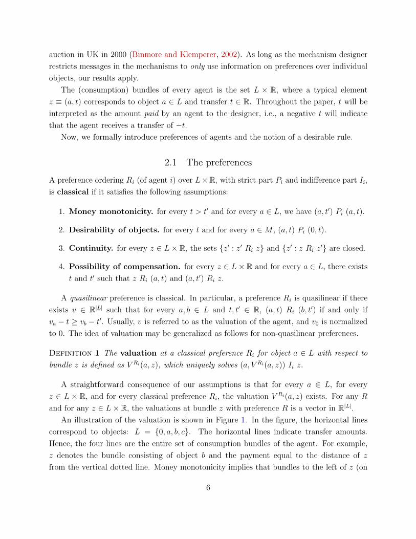
and for any z ∈ L× R, the valuations at bundle z with preference R is a vector in R|L|.An illustration of the valuation is shown in Figure 1. In the figure, the horizontal lines

correspond to objects: L = {0, a, b, c}. The horizontal lines indicate transfer amounts.

Hence, the four lines are the entire set of consumption bundles of the agent. For example,

z denotes the bundle consisting of object b and the payment equal to the distance of z

from the vertical dotted line. Money monotonicity implies that bundles to the left of z (on

6

z ≡ (b; t)

0

a

b

c

V Ri(a; z)

V Ri(c; z)

V Ri(0; z)0

Worse bundles

Better bundles

Figure 1: Valuation at a preference

the same horizontal line) are better than z. A preference Ri can be described by drawing

(non-intersecting) indifference vectors through these consumption bundles (lines). One such

indifference vector passing through z is shown in Figure 1. This indifference vector actually

consists of four points: V Ri(0, z), V Ri(a, z), z ≡ (b, t), V Ri(c, z) as shown. Parts of the curve

in Figure 1 which lie between the consumption bundle lines is useless and has no meaning -

it is only displayed for convenience. As we go to the left along the horizontal lines starting

from any bundle, we get worse bundles (due to money monotonicity). Similarly, bundles to

the right of a particular bundle are better than that bundle. This is shown in Figure 1 with

respect to the indifference vector.

Our modeling of preferences captures income effects even though we do not model in-

come explicitly. Indeed, as transfer changes, the income levels of agents change and this is

automatically reflected in the preferences.

2.2 Desirable rules

Let RC denote the set of all classical preferences and RQ denote the set of all quasilinear

preferences. We will consider an arbitrary class of classical domain R ⊆ RC - we will put

specific restrictions on R later. A preference of agent i is denoted by Ri ∈ R. A preference

profile is a list of preferences R ≡ (R1, . . . , Rn). The usual notations R−i and R−N ′ will

denote a preference profile without the preference of agent i and without the preferences of

agents in N ′ ⊆ N respectively.

7

An object allocation is an n-tuple (a1, . . . , an) ∈ Ln such that no real (non-null) object is

assigned to two agents, i.e., ai 6= aj for all i, j with ai, aj 6= 0. The set of all object allocations

is denoted by A. A (feasible) allocation is an n-tuple ((a1, t1), . . . , (an, tn)) ∈ A × R, where

(ai, ti) is the allocation of agent i. Let Z denote the set of all feasible allocations. For every

allocation (z1, . . . , zn) ∈ Z, we will denote by zi the allocation of any agent i.

An allocation rule or a rule for short is a map f : Rn → Z. Notice that we focus

attention to deterministic rules. A recent paper by Chen et al. (2016) has shown that in

quasilinear domains, there is no loss of generality in restricting attention to deterministic

rules if the seller wants to maximize expected revenue. However, (a) we consider preferences

which are not necessarily quasilinear and (b) we impose extra conditions beyond incentive

compatibility. Hence, it is not clear if the robustness of deterministic rules proved in Chen

et al. (2016) extends to our setting. Our restriction to deterministic rules is purely driven

by simplicity of analysis.

At a preference profile R ∈ Rn, we denote the allocation of agent i in rule f as fi(R) ≡(ai(R), ti(R)), where ai(R) and ti(R) are respectively the object allocated to agent i and the

transfer paid by agent i at preference profile R. We call a(·) and p(·) an object allocation

rule and a payment rule, respectively.

Definition 2 A rule f : Rn → Z is desirable if it satisfies the following properties:

1. Strategy-proofness. for every i ∈ N , for every R−i ∈ Rn−1, and for every Ri, R′i ∈

R, we have

fi(Ri, R−i) Ri fi(R′i, R−i).

2. Ex-post individual rationality (IR). for every i ∈ N , for every R ∈ Rn, we have

fi(R) Ri (0, 0).

3. Equal treatment of equals (ETE). for every i, j ∈ N , for every R ∈ Rn with

Ri = Rj, we have fi(R) Ii fj(R).

4. No wastage (NW). for every R ∈ Rn and for every a ∈M , there exists some i ∈ Nsuch that ai(R) = a.

Out of the four properties of a desirable rule, strategy-proofness and IR are standard

constraints imposed on a rule. Most of the literature considers Bayesian incentive compat-

ibility and interim individual rationality. As a consequence, one ends up working in the

“reduced-form” problems (Border, 1991), and one needs to put additional constraints, com-

monly referred to as “Border constraints”, in the optimization program. The multi-object

8

analogues of the Border constraints are difficult to characterize (Che et al., 2013) - also see

Gopalan et al. (2015) for a computational impossibility of extending the Border inequal-

ities to our problem. Working with strategy-proof and ex-post IR, we get around these

problems. 10

ETE is a very mild form of fairness requirement. It states that two agents with identical

preferences must be assigned bundles to which they should be indifferent. As argued in the

introduction, such minimal notion of fairness is often required by law. The desirability of

NW is debatable, and the readers are referred back to the Introduction section for more

discussions on this. Besides desirability, for some of our results, we will require some form

of restrictions on payments.

Definition 3 A rule f : Rn → Z satisfies no subsidy if for every R ∈ Rn and for every

i ∈ N , we have ti(R) ≥ 0.

No subsidy can be considered desirable to exclude “fake” agents, who participate in mecha-

nisms just to take away available subsidy. As was discussed earlier, it is an axiom satisfied

by most standard mechanisms in practice. No subsidy is motivated by the fact that in many

settings, the seller may not have any means to finance any agents.

3 The minimum Walrasian equilibrium price rule

In this section, we define the notion of a Walrasian equilibrium, and use it to define a desirable

rule. A price vector p ∈ R|L|+ defines a price for every object with p0 = 0. At any price vector

p, let D(Ri, p) := {a ∈ L : (a, pa) Ri(b, pb) ∀ b ∈ L} denote the demand set of agent i with

preference Ri at price vector p. 11

Definition 4 An object allocation (a1, . . . , an) and a price vector p is a Walrasian equi-

librium at a preference profile R ∈ Rn if

1. ai ∈ D(Ri, p) for all i ∈ N and

2. for all a ∈M with ai 6= a for all i ∈ N , we have pa = 0.

10On a related note, in the single object case, there is strong equivalence between the set of strategy-proof

and Bayesian incentive compatible rules (Mookherjee and Reichelstein, 1992; Manelli and Vincent, 2010;

Gershkov et al., 2013). But this equivalence is lost in the multi-object problem.11A more traditional definition of demand set using the notion of a budget set is also possible. Here, we

define the budget set of each agent at price vector p as B(p) := {(a, pa) : a ∈ L} and the demand set of

agent i is just the maximal bundles in the budget set according to preference Ri.

9

We refer to p and {zi ≡ (ai, pai)}i∈N defined above as a Walrasian equilibrium price

vector and a Walrasian equilibrium allocation at R respectively.

Since we assume n > m, the conditions of Walrasian equilibrium implies that for all

a ∈M , we have ai = a for some i ∈ N . 12

A Walrasian equilibrium price vector p is a minimum Walrasian equilibrium price

vector at preference profile R if for every Walrasian equilibrium price vector p′ at R, we

have pa ≤ p′a for all a ∈ L. Demange and Gale (1985) prove that if R is a profile of classical

preferences, then a Walrasian equilibrium exists at R, and the set of Walrasian equilibrium

price vectors forms a lattice with a unique minimum and a unique maximum. We denote the

minimum Walrasian equilibrium price vector at R as pmin(R). Notice that if n > m, then

for every a ∈ A, we have pmina (R) > 0. 13

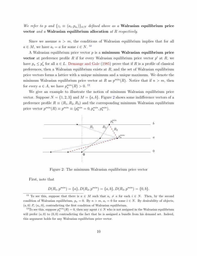
We give an example to illustrate the notion of minimum Walrasian equilibrium price

vector. Suppose N = {1, 2, 3} and M = {a, b}. Figure 2 shows some indifference vectors of a

preference profile R ≡ (R1, R2, R3) and the corresponding minimum Walrasian equilibrium

price vector pmin(R) ≡ pmin ≡ (pmin0 = 0, pmina , pminb ).

00

a

bpminb

pmina

R1 R2R3

Figure 2: The minimum Walrasian equilibrium price vector

First, note that

D(R1, pmin) = {a}, D(R2, p

min) = {a, b}, D(R3, pmin) = {0, b}.

12 To see this, suppose that there is a ∈ M such that ai 6= a for each i ∈ N . Then, by the second

condition of Walrasian equilibrium, pa = 0. By n > m, ai = 0 for some i ∈ N . By desirability of objects,

(a, 0) Pi (ai, 0), contradicting the first condition of Walrasian equilibrium.13To see this, suppose pmin

a (R) = 0, then any agent i ∈ N who is not assigned in the Walrasian equilibrium

will prefer (a, 0) to (0, 0) contradicting the fact that he is assigned a bundle from his demand set. Indeed,

this argument holds for any Walrasian equilibrium price vector.

10

Hence, a Walrasian equilibrium is the allocation where agent 1 gets object a, agent 2 gets

object b, and agent 3 gets the null object at the price vector pmin. Also, pmin is the minimum

such Walrasian equilibrium price vector. To see this, let p be any other Walrasian equilibrium

price vector. If pa < pmina and pb < pminb , then no agent demands the null object, contradicting

Walrasian equilibrium. Thus, pa ≥ pmina or pb ≥ pminb . If pb < pminb , then by pa ≥ pmina ,

both agents 2 and 3 will demand only object b, contradicting Walrasian equilibrium. Thus,

pb ≥ pminb . But, if pa < pmina , both agents 1 and 2 will demand only object a, a contradiction

to Walrasian equilibrium. Hence, p ≥ pmin.

We now describe a desirable rule satisfying no subsidy. The rule picks a minimum Wal-

rasian equilibrium allocation at every profile of preferences. Although the minimum Wal-

rasian equilibrium price vector is unique at every preference profile, there may be multiple

supporting object allocation - all these object allocations must be indifferent to all the agents.

To handle this multiplicity problem, we introduce some notation. Let Zmin(R) denote the

set of all allocations at a minimum Walrasian equilibrium at preference profile R. Note that

if ((a1, . . . , an), p) ∈ Zmin(R) then p = pmin(R).

Definition 5 A rule fmin : Rn → Z is a minimum Walrasian equilibrium price

(MWEP) rule if

fmin(R) ∈ Zmin(R) ∀ R ∈ Rn.

Demange and Gale (1985) showed that every MWEP rule is strategy-proof. 14 Clearly,

it also satisfies individual rationality, no subsidy, and ETE. We document this fact below.

Fact 1 (Demange and Gale (1985); Morimoto and Serizawa (2015)) Every MWEP

rule is desirable and satisfies no subsidy.

4 The results

In this section, we formally state our results. The proofs of our results will be presented in

Section 5. Before we state our result, we define some extra notations and the richness in

domain necessary for our results.

14The MWEP rule satisfies a stronger incentive property called group-strategy-proofness, which means that

no coalition of agents can manipulate this rule.

11

4.1 Richness and ex-post revenue maximization

The domain of preferences that we consider for our first result is the following. 15

Definition 6 A domain of preferences R is rich if for all a ∈M and for every price vector

p with pa > 0, pb = 0 for all b 6= a and for every price vector p > p, there exists Ri ∈ R such

that

D(Ri, p) = {0} and D(Ri, p) = {a}.

Figure 3 illustrates this notion of richness with two objects a and b - two possible price

vectors p and p are shown and two indifference vectors of a preference Ri are shown such

that D(Ri, p) = {0} and D(Ri, p) = {a}.

0

a

bpb

papa

0

pb = 0

RiRi

Figure 3: Illustration of richness

Richness requires that if there are two price vectors p > p, where the only positive price

object at p is object a, then there is a preference ordering where the agent only demands

a at p and demands nothing at p. In quasilinear domain, if the set of valuations is the set

of all positive real numbers, then our richness condition is satisfied - for instance, consider

a quasilinear preference where we pick a value for object a between pa and pa and value for

all other objects arbitrarily close to zero. Later, we show that this richness condition can be

satisfied for many non-quasilinear preferences also.

A closer inspection of the richness reveals that if p is too small, then richness requires

the existence of a preference where the “value” for real objects is very small. In quasilinear

15For every price vector p ∈ R|L|+ , we assume that p0 = 0. Further, for any pair of price vectors p, p ∈ R|L|+ ,

we write p > p if pa > pa for all a ∈M .

12

domain, we can weaken this richness to a weaker condition which requires valuations in an

interval of the form (vmin,∞), where vmin ≥ 0 is any lower bound on the valuation of the

objects. A formal definition and proof is available upon request.

We now formally state our first main result. For any rule f : Rn → Z, we define the

revenue at preference profile R ∈ Rn as

Revf (R) :=∑i∈N

ti(R).

Definition 7 A rule f : Rn → Z is ex-post revenue optimal among a class of rules

defined on Rn if for every rule g in this class, we have

Revf (R) ≥ Revg(R) ∀ R ∈ Rn.

It is not clear that an ex-post revenue optimal rule exists. Our main result shows that

the MWEP rule is ex-post revenue optimal among the class of desirable rules satisfying no

subsidy.

Theorem 1 Suppose R is a rich domain of preferences. Every MWEP rule is ex-post

revenue optimal among the class of desirable rules satisfying no subsidy defined on Rn.

Theorem 1 clearly implies that even if we do expected revenue maximization with respect

to any prior on the preferences of agents, we will only get an MWEP rule among the class

of desirable and no subsidy rules.

Although it is difficult to describe the set of desirable rules satisfying no subsidy, such

rules exist even in the domain of quasilinear preference (which is a rich domain) which are

different from the MPWE rules. We include an example of Tierney (2016) in the supplemen-

tary appendix at the end of this manuscript for completeness. Indeed, the set of all desirable

rules satisfying no subsidy seems quite complicated to describe in the quasilinear domain of

preferences. Our main result shows that every MWEP rule is revenue-optimal in a strong

sense in the class of desirable and no subsidy rules.

4.2 Income effects and no bankruptcy

We now discuss some specific domains where our richness condition holds. We also show

how Theorem 1 can be strengthened in some specific rich domains.

13

Definition 8 A preference Ri satisfies positive income effect if for every a, b ∈ L and

for every t, t′ with t < t′ and (b, t′) Ii (a, t), we have

(b, t′ − δ) Pi (a, t− δ) ∀ δ > 0.

A preference Ri satisfies non-negative income effect if for every a, b ∈ L and for every

t, t′ with t < t′ and (b, t′) Ii (a, t), we have

(b, t′ − δ) Ri (a, t− δ) ∀ δ > 0.

Let R++ and R+ denote the sets of all positive income effect and non-negative income effect

domain of preferences respectively.

A standard definition of positive income effect will say that a preferred object is more

preferred as income increases. In our model, when income increases by δ > 0, the origin of

consumption space moves to right by δ. This movement is equivalent to a decrease of prices

by δ. In the above definition, (b, t′) Ii (a, t) and t′ > t imply that object b is strictly preferred

to object a at any common payment levels t′′ ∈ [t, t′). Then, positive income effect requires

that consumption bundle (b, t′ − δ) is strictly preferred to consumption bundle (a, t− δ).Positive (non-negative) income effects are natural restrictions to impose in settings where

the objects are normal goods. Our next claim shows that the richness condition is satisfied

in a variety of domains containing positive income effect preferences. Since the proof is

straightforward, we skip it.

Claim 1 A domain of preferences R satisfies richness if any of the following conditions

holds: (1) R ⊇ RQ; (2) R ⊇ R+; (3) R ⊇ R++; (4) R ⊇ RC \ RQ.

Next, we show that if the domain contains all the positive income effect preferences, then

our result can be strengthened - we can replace no subsidy in Theorem 1 by the following

no bankruptcy condition.

Definition 9 A rule f : Rn → Z satisfies no bankruptcy if there exists ` ≤ 0 such that

for every R ∈ Rn, we have∑

i∈N ti(R) ≥ `.

Obviously, no bankruptcy is a weaker property than no subsidy. No bankruptcy is motivated

by settings where the seller has limited means to finance the auction participants. Theorem

1 can now be strengthened in the positive income effect domain.

Theorem 2 Suppose R ⊇ R++. Every MWEP rule is ex-post revenue optimal among the

class of desirable rules satisfying no bankruptcy defined on Rn.

14

4.3 Pareto efficiency

Since no wastage is a minimal form of efficiency axiom, it is natural to explore the implications

of stronger forms of efficiency. We now discuss the implications of Pareto efficiency in our

problem and relate it to our results. Before we formally define it, we must state the obvious

fact that no wastage is a much weaker but more testable axiom in practice than Pareto

efficiency. Our results establish that even if a seller maximizes her revenue with this weak

form of efficiency, it will be forced to use a Pareto efficient rule.

Definition 10 A rule f : Rn → Z is Pareto efficient if at every preference profile

R ∈ Rn, there exists no allocation ((a1, t1), . . . , (an, tn)) such that

(ai, ti) Ri fi(R) ∀ i ∈ N∑i∈N

ti ≥ Revf (R),

with either the second inequality holding strictly or some agent i strictly preferring (ai, ti) to

fi(Ri).

The above definition is the appropriate notion of Pareto efficiency in this setting: (a) the

first set of inequalities just say that no agent i prefers the allocation (ai, ti) to that of the rule

and (b) the second inequality ensures that the seller’s revenue is not better in the proposed

allocation. Without the second inequality, there is always an allocation where some money

is distributed to all the agents to make them better off than the allocation in the rule.

The MWEP rule is Pareto-efficient (Morimoto and Serizawa, 2015). An immediate corol-

lary of our results is the following.

Corollary 1 Let f : Rn → Z be a desirable rule. If R is rich and f satisfies no subsidy,

then consider the following statements.

1. f = fmin.

2. Revf (R) ≥ Revf′(R) for any desirable rule f ′ : Rn → Z satisfying no subsidy.

3. f is Pareto efficient.

Statements (1) and (2) are equivalent, and each of them imply Statement (3).

If R ⊇ R+ and f satisfies no bankruptcy, then the same equivalence between (1) and (2)

holds with no subsidy weakened to no bankruptcy in (2), and each of them still imply (3).

15

Proof : The MWEP rule is Pareto efficient - first welfare theorem, see also Morimoto and

Serizawa (2015). This implies (1) ⇒ (3). The equivalence of (1) and (2) follows from

Theorem 1. Hence, (2)⇒ (3).

Similarly, the implications with no bankruptcy follows from Theorem 2. �

In other words, even if the seller maximizes her revenue among the set of all desirable

rules satisfying no subsidy (or no bankruptcy in the positive income effect domain), it will

be forced to use a Pareto efficient rule. Hence, we get Pareto efficiency as a corollary without

imposing it explicitly.

If Pareto efficiency is explicitly imposed, then the following two results are known in the

literature, and using them, we can strengthen Corollary 1 further.

1. In the quasilinear domain, every strategy-proof and Pareto efficient rule is a Groves

rule (Holmstrom, 1979). 16 Imposing individual rationality and no subsidy immedi-

ately implies that the pivotal or the Vickrey-Clarke-Groves (VCG) rule is the unique

strategy-proof rule satisfying Pareto efficiency, individual rationality, and no subsidy

- notice that equal treatment of equals is not needed for this result and no wastage

is implied by Pareto efficiency. The MWEP rule coincides with the VCG rule in the

quasilinear domain.

2. In the classical domain RC (containing all classical preferences), the MWEP rule is

the unique rule satisfying strategy-proofness, individual rationality, Pareto efficiency,

and no subsidy (Morimoto and Serizawa, 2015) - again, equal treatment of equals is

not needed for this result and no wastage is implied by Pareto efficiency.

Both these results imply the following strengthening of Corollary 1 in quasilinear and

classical domains - notice that the corollary may not hold in every rich classical domain.

Corollary 2 Let f : Rn → Z be a desirable rule. If R ∈ {RQ,RC} and f satisfies no

subsidy, then the following statements are equivalent.

1. f = fmin.

2. Revf (R) ≥ Revf′(R) for any desirable rule f ′ : Rn → Z satisfying no subsidy.

3. f is Pareto efficient.

16Such revenue equivalence results usually require some richness in domain, for instance, space of valuations

must be (topologically) connected (Chung and Olszewski, 2007). Such results and our results will fail if we

do not have enough richness - for instance, in discrete domains.

16

4.4 Some examples illustrating necessity of additional axioms

In this section, we give some examples to illustrate the implications of our axioms on the

result.

Notion of incentive compatibility and IR. Consider a rule that chooses the maxi-

mum Walrasian equilibrium allocation at every profile. Such a rule will satisfy no subsidy

and all the properties of desirability except strategy-proofness. Similarly, an MWEP rule

supplemented by a participation fee satisfies no subsidy and all the properties of desirability

except ex-post IR. Both these rules generate more revenue than the MWEP rule. Hence,

strategy-proofness and ex-post IR are necessary for our results to hold.

What is less clear is if we can relax the notion of incentive compatibility to Bayesian

incentive compatibility in our results. For this, consider an example with a single object

and quasilinear preferences. With symmetric agents (i.e., agents having independent and

identical distribution of values), a symmetric Bayesian Nash equilibrium strategy of the first

price auction is increasing and continuous function b(·) of valuations - for an exact expression

of this function, see Krishna (2009). Consider the rule such that for each valuation profile

v = (v1, . . . , vn), the outcome of the bid profile (b(v1), . . . , b(vn)) of the first price auction is

chosen. Call this rule the first-price based rule. It is Bayesian incentive compatible. Though,

the first-price based rule satisfies no subsidy, ex-post individual rationality, and no wastage,

it fails to satisfy ETE (unless, we break ties using uniform randomization). To see this,

if two agents have same value, they bid the same amount in the first-price based rule. If

there is no randomization to break ties, only one of those agents wins the object at his bid

amount, whereas the other agent gets zero payoff. Since bid amount is less than the value

in the first-price based rule, the winner gets positive payoff, and this violates ETE.

However, this can be rectified in two ways. First, whenever there is tie for the winning

bid, all the winning agents get the object with equal probability. This introduces uniform

randomization, and ETE is now satisfied. Hence, the randomized first-price based rule

is Bayesian incentive compatible, satisfies ex-post IR, ETE, no wastage, and no subsidy.

Obviously, there are profiles of values where such a first-price based rule generates more

revenue than the Vickrey rule - winning bid in the first-price auction may be higher than

the second highest value. 17

An alternate approach to restoring ETE in the first-price based rule is to modify it

17 It is well known that the expected revenue from both the auctions is the same. Also, as we discussed

earlier, interim equivalence of strategy-proof and Bayesian incentive compatible rules are known for single

object quasilinear models.

17

in a deterministic manner whenever there is a tie in the winning bids. Consider a profile

of values (v1, . . . , vn) such that more than one agent has bid the highest amount, say, B.

Note that this bid B corresponds to value b−1(B). In such a case, we break the winning

agent tie deterministically by giving the object (with probability 1) to one of the winning

agents. Further, we ask him to pay his value b−1(B). This ensures that the winner and

the losing agents all get a payoff of zero, and thus, it restores ETE. More formally, the rule

corresponding to this modified first-price based rule is the following.

1. Agents submit their values (v1, . . . , vn).

2. If there is a unique highest valued agent i, he is given the object and he pays b(vi),

where b is the unique symmetric Bayesian equilibrium bidding function of the first-price

auction.

3. If there are more than one highest valued agents, then any one of them is given the

object and is asked to pay his value.

Notice that this only modifies the rule corresponding to the first-price auction at zero

measure profiles of values. Hence, the modified first-price based rule is Bayesian incentive

compatible. Further, it is deterministic, satisfies ETE, no wastage, no subsidy, and ex-post

IR. Because of the same reasons given for first-price auction, there are profiles of values

where such a modified first-price based rule generates more revenue than the Vickrey rule.

This illustrates that we cannot relax strategy-proofness to Bayesian incentive compati-

bility in our results.

No wastage. It is easy to see that no wastage is required for our result - in the quasilinear

domain of preferences with one object, Myerson (1981) shows that Vickrey rule with an

optimally chosen reserve price maximizes expected revenue for independent and identically

distributed values of agents. Such a rule wastes the object and generates more revenue than

the Vickrey rule, which is also the MWEP rule, at some profiles of preferences.

No wastage is also necessary in a more indirect manner. Consider the domain of quasi-

linear preferences with two objects M ≡ {a, b} and N = {1, 2, 3}. We show that the seller

may increase her revenue by not selling all the objects. Consider a profile of valuations as

follows:

v1(a) = v1(b) = 5

v2(a) = v2(b) = 4

v3(a) = v3(b) = 1.

18

The MWEP price at this profile is pmina = pminb = 1, which generates a revenue of 2 to the

seller. On the other hand, suppose the seller conducts a Vickrey rule of object a only. Then,

he generates a revenue of 4. Hence, the seller can increase her revenue at some profiles of

valuations by withholding objects. Notice that withholding objects is a stronger violation of

efficiency, and is easier to detect than misallocating the objects among agents.

In allocating public assets, governments are supposed to pursuit several goals such as

revenue and efficiency. Usually, revenue and efficiency are not compatible. No wastage is

a mild requirement on efficiency and our result shows how revenue maximization can be

reconciled with efficiency using no wastage.

Equal treatment of equals. Consider an example with one object and two agents in

the quasilinear domain of preferences. Hence, the preference of each agent i ∈ {1, 2} can

be described by his valuation for the object vi. Note that the MWEP rule collapses to the

Vickrey rule for this problem.

We define the following rule: the object is first offered to agent 1 at price p > 0; if agent

1 accepts the offer, then he gets the object at price p and agent 2 does not get anything and

does not pay anything; else, agent 2 is given the object for free.

This rule generates a revenue of p whenever v1 ≥ p (but generates zero revenue other-

wise). However, note that the Vickrey rule generates a revenue of v2 when v1 > v2. Hence,

if p > v2, then this rule generates more revenue that the Vickrey rule. Also, notice that this

rule satisfies no subsidy and all the properties of desirability except equal treatment of equals.

No subsidy. It is tempting to conjecture that no subsidy can be relaxed in quasilinear

domain of preferences. A natural approach to prove this is to use Theorem 1, which applies

to the quasilinear domain, in the following way: (1) For every desirable rule, we construct

another desirable rule which satisfies no subsidy and generates more revenue; (2) Use The-

orem 1 to arrive at the conclusion that the MWEP rule is revenue-optimal in the class of

desirable rule. The first step does not quite work. In the quasilinear domain, every desirable

rule can be converted to a strategy-proof, individually rational, and no subsidy rule using

“multidimensional” versions of revenue equivalence formula (Jehiel et al., 1999; Krishna and

Maenner, 2001; Milgrom and Segal, 2002; Chung and Olszewski, 2007; Heydenreich et al.,

2009). But such a transformation may not preserve equal treatment of equals. As a result,

we cannot apply Step (2) any more. We now give a concrete example to illustrate that our

result does not hold without no subsidy.

For the example, consider one object and two agents in the quasilinear domain - hence,

19

preferences of agents can be represented by their valuations v1 and v2. Further, assume that

valuations lie in R++. Choose k ∈ (0, 1) and define the rule f ≡ (a, t) as follows: for every

(v1, v2)

a(v1, v2) =

{(1, 0) if kv1 > v2,

(0, 1) otherwise,

t1(v1, v2) =

{−(v2 − kv2) if a1(v1, v2) = 0,v2k− (v2 − kv2) if a1(v1, v2) = 1,

t2(v1, v2) =

{0 if a2(v1, v2) = 0,

kv1 if a2(v1, v2) = 1.

It is straightforward to check that the object allocation rule a is monotone (i.e., fixing the

valuation of one agent, if valuation of the other agent is increased, his allocation probability

increases) and payments satisfy the revenue equivalence formula, and hence, the rule is

strategy-proof (a more direct proof is also possible). It is also not difficult to see that utilities

of the agents are always non-negative, and hence, individual rationality holds. Finally, if

v1 = v2, we have

a1(v1, v2) = 0, a2(v1, v2) = 1, t1(v1, v2) = −(v2 − kv2), t2(v1, v2) = kv1.

Hence, net utility of agent 1 is v2− kv2 and that of agent 2 is v1− kv1, which are equal since

v1 = v2. This shows that the rule satisfies equal treatment of equals.

However, the rule pays agent 1 when he does not get the object. Thus, it violates no

subsidy. The revenue from this rule when kv1 > v2 is

v2

(1

k+ k − 1

)≥ v2.

The Vickrey rule generates a revenue of v2 when kv1 > v2. Hence, this rule generates more

revenue than the Vickrey rule when kv1 > v2. This shows that we cannot drop no subsidy

from Theorem 1. 18

4.5 Discussions on applicability of the results

As discussed in the introduction, our results are driven by a particular set of assumptions we

have made in the paper, which are different from the literature. Here, we give two real-life

18 Further inspection reveals that the revenue from this rule when v1 = v2 = v is kv−v(1−k) = v(2k−1).

So, if k < 12 , this revenue approaches −∞ as v →∞. Hence, this rule even violates no bankruptcy.

20

examples of allocation problems, where most of the assumptions made in the paper appear

to make sense.

Indian Premier League auctions. A professional cricket league, called the Indian Pre-

mier League (IPL) was started in India in 2007. 19 Eight Indian cities were chosen and it

was decided to have a team from each of those cities (i.e., eight heterogeneous objects were

sold). An auction was held to sell these teams to interested owners (bidders). The auctions,

whose details are not available in public domain, fetched more than 700 million US Dollars

in revenue to IPL. Clearly, it does not make sense for two teams to have the the same owner

- so, the unit demand assumption in our model is satisfied in this problem. The huge sums

of bids implied that most of these teams were financed out of loans from banks, which im-

plies non-quasilinear preferences of bidders. Further, when IPL was starting out, it must be

interested in starting with teams in as many cities as possible - else, it would have sent a

wrong signal to its future prospects. Indeed, all the teams were sold with high bid prices.

So, a natural objective for IPL seems to be revenue maximization with no wastage. Finally,

as is common in such settings, IPL did not subsidize any bidders.

Online advertisement auctions. Google sells billions of dollars worth of keywords using

auctions for advertisement slots (Edelman et al., 2007; Varian, 2009). Many other search

engines also sell display advertisement slots on webpages, which are auctioned as soon as web

pages are displayed (Lahaie et al., 2008; Ghosh et al., 2009). Usually, each advertisement

slot is awarded a unique bidder - so, the unit demand assumption is satisfied. 20 It is not

clear whether Google uses reserve prices or not, but there is widespread belief that Google

aims to be efficient. 21 However, it is fair to say that Google aims to maximize revenue from

its sale of advertisement slots. The bidders are usually given a fixed budget to work with,

and this results in an extreme form of non-quasilinearity. This has started a big literature on

auctions with budget constraints in the computer science community (Ashlagi et al., 2010;

Dobzinski et al., 2012; Lavi and May, 2012). Finally, Google does not subsidize any of its

bidders.

19Interested readers can read the Wiki entry for IPL: https://en.wikipedia.org/wiki/Indian_Premier_League

and a news article here: http://content-usa.cricinfo.com/ipl/content/current/story/333193.html.20The analysis of this problem has been done under the unit demand assumption in the literature (Edelman

et al., 2007; Varian, 2009).21See this issue being discussed in a blog post by Noam Nisan:

https://agtb.wordpress.com/2009/06/09/revenue-vs-efficiency-in-auctions/

21

Another example that fits our model is the allocation of public housing to citizens in

different countries (Andersson and Svensson, 2014; Andersson et al., 2016), where houses

are allocated to agents with unit demand constraint. These examples reinforce the fact that

even though a precise description to revenue maximizing multi-object auction is impossible

in many settings, for a variety of problems where no wastage makes sense, the MWEP rule

is a strong candidate.

In the two examples above, the seller is not the Government. It makes more sense for

such a seller to maximize her revenue. Corollaries 1 and 2 establish that even if such a seller

maximizes her revenue, under desirability and no subsidy she would be forced to pick an

MWEP rule, which is Pareto efficient.

5 The proofs

In this section, we present all the proofs. The proofs, though tedious and far from trivial,

do not require any sophisticated mathematical tool. This is an added advantage of our ap-

proach, and makes the results even more surprising. The proofs use the following fact very

crucially: the MWEP rule chooses a Walrasian equilibrium outcome. 22

Intuitions. Before diving into the proofs, we want to stress here that a greedy approach

of proving our results would be to first prove that any desirable rule satisfying no subsidy

and maximizing revenue must be Pareto efficient. In the quasilinear domain, using revenue

equivalence will then pin down the MWEP (VCG) rule. This approach will fail in our setting

because our results work even without quasilinearity and revenue equivalence does not hold

in such domains. Our proofs work by showing various implications of desirability and no

subsidy on consumption bundles of agents. It uses richness of the domain to derive these im-

plications. In that sense, it departs from traditional Myersonian techniques, where revenue

maximization is a programming problem with object allocation rules as decision variables.

This also means that our proof is less intuitive than standard approaches for quasilinear

preference domain.

We start off by showing an elementary lemma which shows that if a desirable rule gives

every agent weakly better consumption bundles than an MWEP rule at every preference

22With quasilinear preferences, if valuations of agents satisfy the gross substitutes property, then a minimum

Walrasian equilibrium price vector exists, but it is no longer strategy-proof (Gul and Stacchetti, 1999). Hence,

it is not clear if our results can be extended to such a model. We leave this as an open question.

22

profile, then its revenue is less than the MWEP rule. This lemma will be used to prove both

our results.

Lemma 1 For every desirable rule f : Rn → Z, where R is a rich domain, and for every

R ∈ Rn, the following holds:[fi(R) Ri f

mini (R) ∀ i ∈ N

]⇒[Revf

min

(R) ≥ Revf (R)],

where fmin is an MWEP rule.

Proof : Fix a profile of preferences R and denote fmin(R) ≡ (z1, . . . , zn), where for each i ∈N , zi ≡ (ai, p

minai

(R)). Now, for every i ∈ N , we have fi(R) ≡ (ai(R), ti(R)) Ri (ai, pminai

(R))

and by the Walrasian equilibrium property, (ai, pminai

(R)) Ri (ai(R), pai(R)). This gives us

ti(R) ≤ pai(R) for each i ∈ N . Hence,

Revf (R) =∑i∈N

ti(R) ≤∑i∈N

pai(R) = Revfmin

(R),

where the last equality follows from the fact that all the objects with positive price are

allocated in a Walrasian equilibrium and f also allocates all the objects (because of no

wastage). �

5.1 Proof of Theorem 1

We start with a series of Lemmas before providing the main proof. Throughout, we assume

that R is a rich domain of preferences and f is a desirable rule satisfying no subsidy on

Rn. For the lemmas, we need the following definition. A preference Ri is (a, t)-favoring

for t > 0 and a ∈ M if for price vector p with pa = t, pb = 0 for all b 6= a, we have

D(Ri, p) = {a}. An equivalent way to state this is that Ri is (a, t)-favoring for t > 0 and

a ∈M if V Ri(b, (a, t)) < 0 for all b 6= a.

Lemma 2 For every preference profile R, for every i ∈ N with fi(R) 6= 0, and for every R′isuch that R′i is an fi(R)-favoring preference, we have fi(R

′i, R−i) = fi(R).

Proof : If ai(R′i, R−i) = ai(R), then strategy-proofness implies ti(R

′i, R−i) = ti(R), and we

are done. Suppose a = ai(R) 6= ai(R′i, R−i) = b. By strategy-proofness,[

(b, ti(R′i, R−i)) R

′i (a, ti(R))

]⇒

[ti(R

′i, R−i) ≤ V R′i(b, (a, ti(R)))

].

Since R′i is (a, ti(R))-favoring, we must have V R′i(b, (a, ti(R))) < 0. This implies that

ti(R′i, R−i) < 0, which is a contradiction to no subsidy. �

23

Lemma 3 For every preference profile R and for every i ∈ N with fi(R) 6= 0, there is no

j 6= i such that Rj is fi(R)-favoring.

Proof : Assume for contradiction that there is j 6= i such that Rj is fi(R)-favoring. Consider

R′i ≡ Rj. By equal treatment of equals fi(R′i, R−i) Ij fj(R

′i, R−i). Also, by Lemma 2,

fi(R′i, R−i) = fi(R). Hence, fi(R) Ij fj(R

′i, R−i). Note that a = ai(R) = ai(R

′i, R−i) 6=

aj(R′i, R−i) = b. Then, tj(R) = V Rj(b, fi(R)) < 0, where the strict inequality followed from

the fact that Rj is fi(R)-favoring and b 6= ai(R). But this contradicts no subsidy. �

Lemma 4 For every preference profile R, for every i ∈ N , for every (a, t) with a = ai(R) 6= 0

and t > 0, if there exists j 6= i such that Rj is (a, t)-favoring, then ti(R) > t.

Proof : Suppose ti(R) ≤ t. Since Rj is (a, t)-favoring, ti(R) ≤ t implies that Rj is also

fi(R) ≡ (a, ti(R))-favoring. This is a contradiction to Lemma 3. �

For the proof, we use a slightly stronger version of (a, t)-favoring preference.

Definition 11 For every bundle (a, t) with t > 0 and for every ε > 0, a preference Ri ∈ Ris a (a, t)ε-favoring preference if it is a (a, t)-favoring preference and

V Ri(a, (0, 0)) < t+ ε

V Ri(b, (0, 0)) < ε ∀ b ∈M \ {a}.

The following lemma shows that if R is rich, then (a, t)ε-favoring preferences exist for

every (a, t) and ε.

Lemma 5 Suppose R is rich. Then, for every bundle (a, t) with t > 0 and for every ε > 0,

there exists a preference Ri ∈ R such that it is (a, t)ε-favoring.

Proof : Define p as follows:

pa = t, pb = 0 ∀ b 6= a.

Define p as follows:

pa = t+ ε, p0 = 0, pb = ε ∀ b ∈M \ {a}.

By richness, there exists Ri such that D(Ri, p) = {a} and D(Ri, p) = {0}. But this implies

that Ri is (a, t)-favoring and

V Ri(a, (0, 0)) < t+ ε

V Ri(b, (0, 0)) < ε ∀ b ∈M \ {a}.

24

Hence, Ri is (a, t)ε-favoring. �

We will now prove Theorem 1 using these lemmas.

Proof of Theorem 1

Proof : Fix a desirable rule f : Rn → Z satisfying no subsidy, where R is a rich domain of

preferences. Fix a preference profile R ∈ Rn. Let (z1, . . . , zn) ≡ fmin(R) be the allocation

chosen by an MWEP rule fmin at R. For simplicity of notation, we will denote zj ≡ (aj, pj),

where pj ≡ pminaj(R), for all j ∈ N . We prove that fi(R) Ri zi for all i ∈ N , and by Lemma

1, we will be done.

To prove that fi(R) Ri zi for all i ∈ N , assume for contradiction that there is some agent,

without loss of generality agent 1, such that z1 P1 f1(R). We first construct a finite sequence

of agents and preferences (i1, R′i1

), (i2, R′i2

), . . . , (in, R′in) satisfying certain properties. For no-

tational convenience, we denote this sequence as (1, R′1), . . . , (n,R′n). This sequence satisfies

the properties that for every k ∈ {1, . . . , n},

1. zk Pk fk(R) if k = 1 and zk Pk fk(R′Nk−1

, R−Nk−1) if k > 1, where Nk−1 ≡ {1, . . . , k−1}.

2. ak 6= 0,

3. R′k is zεk-favoring for some ε > 0 but arbitrarily close to zero.

Now, we construct this sequence inductively.

Step 1 - Constructing (1, R′1). Pick ε > 0 but arbitrarily close to zero and consider a

zε1-favoring preference R′1 - by Lemma 5, such R′1 can be constructed. By our assumption,

z1 P1 f1(R). Suppose a1 = 0. Then, z1 = (0, 0) P1 f1(R), which contradicts individual

rationality. Hence, a1 6= 0.

Step 2 - Constructing (k,R′k) for k > 1. We proceed inductively - suppose, we have already

constructed (1, R′1), . . . , (k − 1, R′k−1) satisfying Properties (1), (2), and (3). Consider agent

j such that aj(R′Nk−1

, R−Nk−1) = ak−1.

If j = k − 1, then individual rationality implies that

tk−1(R′Nk−1

, R−Nk−1) ≤ V R′k−1(ak−1, (0, 0)) < pk−1 + ε,

where the last inequality followed from the fact that R′k−1 is (zk−1)ε-favoring. Further, by

our induction hypothesis, zk−1 Pk−1 fk−1(R′Nk−2

, R−Nk−2), and we get

pk−1 < V Rk−1(ak−1, fk−1(R′Nk−2

, R−Nk−2)).

25

Since ε is arbitrarily close to zero, we get tk−1(R′Nk−1

, R−Nk−1) < V Rk−1(ak−1, fk−1(R

′Nk−2

, R−Nk−2)).

But this implies that fk−1(R′Nk−1

, R−Nk−1) Pk−1 fk−1(R

′Nk−2

, R−Nk−2), which contradicts strategy-

proofness. Hence, j 6= k − 1.

If j ∈ Nk−2, then by individual rationality, we get tj(R′Nk−1

, R−Nk−1) ≤ V R′j(ak−1, (0, 0)) <

ε, where the last inequality followed from the fact that R′j is (zj)ε-favoring and j 6= (k − 1).

Since ε is arbitrarily close to zero, we get

tj(R′Nk−1

, R−Nk−1) < ε < pk−1. (1)

But, notice that agent (k − 1) 6= j and R′k−1 is zk−1-favoring (since it is (zk−1)ε-favoring).

Further aj(R′Nk−1

, R−Nk−1) = ak−1. Then, Lemma 4 implies that tj(R

′Nk−1

, R−Nk−1) > pk−1,

which is a contradiction to Inequality 1.

Thus, we have established j /∈ Nk−1. Hence, we denote j ≡ k, and note that

zk Rk zk−1 Pk fk(R′Nk−1

, R−Nk−1),

where the first inequality follows from the Walrasian equilibrium property and the sec-

ond follows from the fact that ak(R′Nk−1

, R−Nk−1) = ak−1 and pk−1 < tk−1(R

′Nk−1

, R−Nk−1)

(Lemma 4). Hence Property (1) is satisfied for agent k. Next, if ak = 0, then (0, 0) =

zk Pk fk(R′Nk−1

, R−Nk−1) contradicts individual rationality. Hence, Property (2) also holds.

Now, we satisfy Property (3) by constructing R′k, which is zεk-favoring for some ε > 0 but

arbitrarily close to zero - by Lemma 5, such R′k can be constructed.

Thus, we have constructed a sequence (1, R′1), . . . , (n,R′n) such that ak 6= 0 for all k ∈ N .

This is impossible since n > m, giving us the required contradiction. �

5.2 Proof of Theorem 2

We now fix a desirable rule f : Rn → Z, where R ⊇ R+. Further, we assume that f satisfies

no bankruptcy, where the corresponding bound as ` ≤ 0. We start by proving an analogue

of Lemma 4.

Lemma 6 For every preference profile R ∈ Rn, for every i ∈ N , and every (a, t) ∈M ×R+

with a = ai(R) 6= 0 and t > 0, if there exists j 6= i such that

V Rj(b, (a, t)) < −n(

maxk∈N

maxc∈M

V Rk(c, (0, 0)))

+ `,

then ti(R) > t.

26

Proof : Assume for contradiction ti(R) ≤ t. Consider R′i = Rj. By strategy-proofness,

fi(R′i, R−i) R

′i fi(R) = (a, ti(R)). By equal treatment of equals,

fj(R′i, R−i) Ij fi(R

′i, R−i) Rj (a, ti(R)).

Note that either ai(R′i, R−i) 6= a or aj(R

′i, R−i) 6= a. Without loss of generality, assume that

aj(R′i, R−i) = b 6= a. Then, using the fact that (b, tj(R

′i, R−i)) Rj (a, ti(R)) and ti(R) ≤ t,

we get

tj(R′i, R−i) ≤ V Rj(b, (a, ti(R)))

≤ V Rj(b, (a, t))

< −n(

maxk∈N

maxc∈M

V Rk(c, (0, 0)))

+ `.

By individual rationality

ti(R′i, R−i) ≤ V R′i(ai(R

′i, R−i), (0, 0)) ≤ max

c∈MV R′i(c, (0, 0)).

Further, individual rationality also implies that for all k /∈ {i, j},

tk(R′i, R−i) ≤ V Rk(ai(R

′i, R−i), (0, 0)) ≤ max

c∈MV Rk(c, (0, 0)).

Adding these three sets of inequalities above, we get∑k∈N

tk(R′i, R−i)

< −n(

maxk∈N

maxc∈M

V Rk(c, (0, 0)))

+ `+ maxc∈M

V R′i(c, (0, 0)) +∑

k∈N\{i,j}

maxc∈M

V Rk(c, (0, 0))

= −n(

maxk∈N

maxc∈M

V Rk(c, (0, 0)))

+ `+ maxc∈M

V Rj(c, (0, 0)) +∑

k∈N\{i,j}

maxc∈M

V Rk(c, (0, 0))

≤ −n(

maxk∈N

maxc∈M

V Rk(c, (0, 0)))

+ (n− 1)(

maxk∈N\{i}

maxc∈M

V Rk(c, (0, 0)))

+ `

≤ −n(

maxk∈N

maxc∈M

V Rk(c, (0, 0))− maxk∈N\{i}

maxc∈M

V Rk(c, (0, 0)))

+ `

≤ `.

This contradicts no bankruptcy. �

Using Lemma 6, we can mimic the proof of Theorem 1 to complete the proof of Theorem

2. We start by defining a class of positive income effect preferences by strengthening the

notion of (a, t)ε-favoring preference. For every (a, t) ∈M ×R+, for each ε > 0, and for each

δ > 0, define R((a, t), ε, δ) be the set of preferences such that for each Ri ∈ R((a, t), ε, δ),

the following holds:

27

1. Ri is (a, t)ε-favoring and

2. V Ri(b, (a, t)) < −δ for all b 6= a.

A graphical illustration of Ri is provided in Figure 4. Since δ > 0, it is clear that a Ri

can be constructed in R((a, t), ε, δ) such that it exhibits positive income effect. Hence,

R+ ∩R((a, t), ε, δ) 6= ∅.

0

a

b

c

t

0−δ ϵ t+ ϵ

RiRi

Figure 4: Illustration of Ri

Proof of Theorem 2

Proof : Now, we can mimic the proof of Theorem 1. We only show parts of the proof that

requires some change. As in the proof of Theorem 1, by Lemma 1, we only need to show that

for every profile of preferences R and for every i ∈ N , fmini (R) Ri f(R), where fmin is an

MWEP rule. Assume for contradiction that there is some profile of preferences R and some

agent, without loss of generality agent 1, such that z1 P1 f1(R), where (z1, . . . , zn) ≡ fmin(R)

be the allocation chosen by the MWEP rule at R. For simplicity of notation, we will denote

zj ≡ (aj, pj), where pj ≡ pminaj(R), for all j ∈ N .

Define δ > 0 as follows:

δ := n(

maxk∈N

maxc∈M

V Rk(c, (0, 0)))− `.

We first construct a finite sequence of agents and preferences: (1, R′1), (2, R′2), . . . , (n,R

′n)

such that for every k ∈ {1, . . . , n},

28

1. zk Pk fk(R) if k = 1 and zk Pk fk(R′Nk−1

, R−Nk−1) if k > 1, where Nk−1 ≡ {1, . . . , k−1}.

2. ak 6= 0,

3. R′k ∈ R+ ∩R(zk, ε, δ) for some ε > 0 but arbitrarily close to zero.

Now, we can complete the construction of this sequence inductively as in the proof of

Theorem 1 (using Lemma 6 instead of Lemma 4), giving us the desired contradiction. �

6 Relation to the literature

Our paper is related to two strands of literature in mechanism design: (1) multi-object

revenue maximization literature and (2) literature on object allocation problem without

quasilinearity. We discuss them in some detail below.

Revenue maximization literature. Ever since the work of Myerson (1981), various ex-

tensions of his work to multi-object case have been attempted in quasilinear domain. Most

of these extensions focus on the single agent (or, screening problem of a monopolist) with

additive valuations (value for a bundle of objects is the sum of values of objects). Arm-

strong (1996, 2000) are early papers that show the difficulty in extending Myerson’s optimal

mechanisms to multiple objects case - he identifies optimal mechanisms for the cases where

agents’ preferences are binary, i.e, the valuations of each agent on a given object are only low

and high values, but demonstrates that it is too complicated to identify optimal mechanisms

for other cases. 23 Rochet and Chone (1998) show how to extend the convex analysis tech-

niques in Myerson’s work to multidimensional environment and point out various difficulties

in the derivation of an optimal mechanism. These difficulties are more precisely formulated

in the following line of work for the single agent additive valuation case: (1) optimal mecha-

nism may require randomization (Thanassoulis, 2004; Manelli and Vincent, 2007); (2) simple

mechanism like selling each good separately (Daskalakis et al., 2016) and selling all the goods

as a grand bundle (Manelli and Vincent, 2006) are optimal for very specific distributions;

(3) there is inherent revenue non-monotonicity of the optimal mechanism - if we take two

distributions with one first-order stochastic-dominating the other, the optimal mechanism

revenue may not increase (Hart and Reny, 2015); (4) the optimal mechanism may require

an infinite menu of prices (Hart and Nisan, 2013).

23Whenever we say optimal mechanisms, we mean, like in Myerson (1981), an expected revenue maximizing

mechanism under incentive and participation constraints with respect to some prior distribution.

29

Since these extensions are for a single agent who has additive valuation for bundles of ob-

jects, this may give the impression that the multi-object optimal mechanism design problem

is difficult only when agents can be allocated more than one object. However, this impression

is not true - the source of the problem is the multiple dimension of private information, which

continues to exist even in the unit demand model considered in our paper. In our model,

even with quasilinearity, the multiple dimensions of private information will be valuations

for each object. As illustrated in Armstrong (1996, 2000), the multiple dimensions of private

information implies that the incentive constraints become complicated to handle. In quasi-

linear domain, the Myersonian approach to this problem would pin down payments of agents

in terms of object allocation rules using the well known revenue equivalence formula (Krishna

and Maenner, 2001; Milgrom and Segal, 2002). Then, the objective function (maximizing

sum of expected payments) is rewritten in terms of object allocation rule. On the constraint

side, necessary and sufficient conditions are identified for the object allocation rule to be im-

plementable (Rochet, 1987; Jehiel et al., 1999; Bikhchandani et al., 2006), and they are put

as constraints. Whether agents can be allocated at most one object or multiple objects, the

multidimensional nature of private information makes both the revenue equivalence formula

and the constraints of the optimization problem become extremely difficult to handle. Vohra

(2011) provides a linear programming approach to study such multidimensional mechanism

design problems and points out similar difficulties.

Further, it is unclear how some of the above single agent results can be extended to

the case of multiple agents. In the multiple agent problems, the set of feasible alloca-

tions starts interacting with the incentive constraints of the agents. Further, the standard

Bayesian incentive compatibility constraints become challenging to handle. Note that in the

single agent problem, these notions of incentive compatibility are equivalent, and for one-

dimensional mechanism design problems, they are equivalent in a useful sense (Manelli and

Vincent, 2010; Gershkov et al., 2013). Because we work in a model without quasilinearity,

we are essentially operating in an “infinite” dimensional mechanism design problem. Hence,

we should expect the problems discussed in quasilinear environment to appear in an even

more complex way in our model.

To circumvent the difficulties from the multidimensional private information and multiple

agents, a literature in computer science has developed approximately optimal mechanisms for

our model - multiple objects and multiple agents with unit demand agents (but with quasilin-

earity). Contributions in this direction include Chawla et al. (2010a,b); Briest et al. (2010);

Cai et al. (2012). Many of these approximate mechanisms allow for randomization. Fur-

ther, these approximately optimal mechanisms involve reserve prices and violate no wastage

30

axiom. It is unlikely that these results extend to environments without quasilinearity.

Finally, the Myersonian approach may not work if preferences are not quasilinear. In a

companion paper (Kazumura et al., 2017), we investigate mechanism design without quasi-

linearity more abstractly and illustrate the difficulty of solving the single object optimal

mechanism design problem. Hence, solving for full optimality without imposing the addi-

tional axioms that we put seems to be even more challenging in our model. In that sense,

our results provide a useful resolution to this complex problem.

Our work can be connected to a beautiful result by Bulow and Klemperer (1996) and

its extension by Roughgarden et al. (2015). In Bulow and Klemperer (1996), it was shown

that (under standard independent and identical agent assumption with regular distribution)

a single object optimal mechanism (with quasilinear preferences) for n agents generates less

expected revenue than a single object Vickrey rule for (n + 1) agents. Hence, if the cost of

recruiting an agent is small, then the Vickrey rule can be recommended. 24 This result has

been extended to our multi-object unit-demand agent setting with quasilinear preferences:

the expected revenue maximizing mechanism for n agents generates less expected revenue

than the VCG rule for (m+n) agents, where m is the number of objects (Roughgarden et al.,

2015) - note that the MWEP rule is the VCG rule in the quasilinear domain. Combined

with our result, we can strengthen this result in quasilinear domain as follows. For every

desirable and no subsidy rule for (m+n) agents, consider the difference between its expected

revenue and the maximum expected revenue for n agents. This difference is non-negative

and is maximized by the VCG (MWEP) rule. 25

Non-quasilinearity literature. There is a short but important literature on object al-

location problem with non-quasilinear preferences. Baisa (2016a) considers the single object

model and allows for randomization with non-quasilinear preferences. He introduces a novel

rule in his setting and studies its optimality properties (in terms of revenue maximization).

We do not consider randomization and our solution concept is different from his. Further,

ours is a model with multiple objects.

The literature with non-quasilinear preferences and multiple objects have traditionally

24Of course, one can argue that if we have (n + 1) agents, then the seller must use the expected revenue

maximizing rule for (n + 1) agents. The main point in Bulow and Klemperer (1996) is that the Vickrey

rule is a prior-free robust rule, whereas the expected revenue maximizing mechanism requires knowledge of

priors.25The computer science literature is interested in such prior-free bounds on optimal multidimensional

rules (which is hard to compute) - a recent paper by Eden et al. (2017) provide further extensions of Bulow-

Klemperer results in multi-object environments where buyers can consume more than one object but have

additive valuations.

31

looked at Pareto efficient rules. As discussed earlier, the closest paper is Morimoto and

Serizawa (2015) who consider the same model as ours. They characterize the MWEP rule

using Pareto efficiency, individual rationality, incentive compatibility, and no subsidy when

the domain includes all classical preferences - see an extension of this characterization in a

smaller domain in Zhou and Serizawa (2016). Pareto efficiency and the complete class of

classical preferences play a critical role in pinning down the MWEP rule in these papers. As

Tierney (2016) points out, even in the quasilinear domain of preferences, there are desirable

rules satisfying no subsidy which are different from the MWEP rule. By imposing revenue

maximization as an objective instead of Pareto efficiency, we get the MWEP rule in our

model. Pareto efficiency is obtained as an implication (Corollaries 1 and 2). Finally, our

results work for not only the complete class of classical preferences, but for a large variety

of domains, such as the class of all quasilinear preferences, one including all non-quasilinear

preferences, one including all preferences exhibiting positive income effects, etc.

Tierney (2016) considers axioms like no discrimination, welfare continuity, and some

stronger form of strategy-proofness to give various characterizations of the MWEP rule with

reserve prices in the quasilinear domain. Using our result, he shows that in the quasilinear

domain, the MWEP rule is the unique rule satisfying strategy-proofness, no-discrimination,

individual rationality, no wastage, and welfare continuity.

In the single object model, earlier papers have carried out axiomatic treatment similar to

Morimoto and Serizawa (2015) - work along this line includes Saitoh and Serizawa (2008);

Sakai (2008, 2013b,a); Adachi (2014); Ashlagi and Serizawa (2012).

When the set of preferences include all or a very rich class of non-quasilinear prefer-

ences and we consider multi-object model where agents can consume more than one object,

strategy-proofness and Pareto efficiency (along with other axioms) have been shown to be

incompatible - (Kazumura and Serizawa, 2016) show this for multi-object allocation prob-

lems where agents can be allocated more than one object; (Baisa, 2016b) shows this for

homogeneous object allocation problems; and Dobzinski et al. (2012); Lavi and May (2012)

show similar results for hard budget-constrained model of a single object. Pareto efficiency

along with other axioms play a crucial role in such impossibility results.

There is a literature in mechanism design and algorithmic game theory on single object

allocation problem with budget-constrained agents - see Che and Gale (2000); Pai and Vohra

(2014); Ashlagi et al. (2010); Lavi and May (2012). The budget-constraint in these papers

introduces a particular form of non-quasilinearity in preferences of agents. Further, the

budget-constraint in these models is hard, i.e., the utility from any payment above the budget

is minus infinity. This assumption is not satisfied by the preferences considered in our model

32

since it leads to discontinuities. Further, these papers focus on single object model.

7 Conclusion

We circumvent the technical difficulties of designing optimal rule in multi-object allocation

problem by imposing additional axioms on rules. We believe that these additional axioms

are appealing in a variety of environment. A consequence of these assumptions is that we

provide robust recommendations on revenue maximizing rule: the MWEP rule is revenue-

maximal profile-by-profile, and the preferences of agents need not be quasilinear. Our proofs

are elementary and without any convex analysis techniques used in the literature. Whether

we can weaken some of these axioms and further strengthen our results is a question for

future research.

References

Adachi, T. (2014): “Equity and the Vickrey allocation rule on general preference domains,”

Social Choice and Welfare, 42, 813–830.

Andersson, T., L. Ehlers, and L.-G. Svensson (2016): “Transferring ownership of

public housing to existing tenants: A market design approach,” Journal of Economic

Theory, 165, 643–671.

Andersson, T. and L.-G. Svensson (2014): “Non-Manipulable House Allocation With

Rent Control,” Econometrica, 82, 507–539.

Armstrong, M. (1996): “Multiproduct nonlinear pricing,” Econometrica, 64, 51–75.

——— (2000): “Optimal multi-object auctions,” The Review of Economic Studies, 67, 455–

481.

Ashenfelter, O. and K. Graddy (2003): “Auctions and the price of art,” Journal of

Economic Literature, 41, 763–787.

Ashlagi, I., M. Braverman, A. Hassidim, R. Lavi, and M. Tennenholtz (2010):

“Position auctions with budgets: Existence and uniqueness,” The BE Journal of Theoret-

ical Economics, 10.

Ashlagi, I. and S. Serizawa (2012): “Characterizing Vickrey Allocation Rule by

Anonymity,” Social Choice and Welfare, 38, 531–542.

33

Ausubel, L. M. and P. Milgrom (2002): “Ascending auctions with package bidding,”

Frontiers of Theoretical Economics, 1, 1–42.

Baisa, B. (2016a): “Auction design without quasilinear preferences,”Theoretical Economics,

12, 53–78.

——— (2016b): “Efficient Multi-unit Auctions for Normal Goods,” Available at SSRN

2824921.

Bikhchandani, S., S. Chatterji, R. Lavi, A. Mualem, N. Nisan, and A. Sen

(2006): “Weak Monotonicity Characterizes Deterministic Dominant Strategy Implemen-

tation,” Econometrica, 74, 1109–1132.

Binmore, K. and P. Klemperer (2002): “The biggest auction ever: the sale of the

British 3G telecom licences,” The Economic Journal, 112, C74–C76.

Blumrosen, L. and N. Nisan (2007): “Combinatorial auctions,” in Algorithmic Game

Theory, ed. by N. Nisan, T. Roughgarden, E. Tardos, and V. V. Vazirani, Cambridge:

Cambridge University Press, chap. 28, 699–716.

Border, K. C. (1991): “Implementation of reduced form auctions: A geometric approach,”

Econometrica, 59, 1175–1187.

Briest, P., S. Chawla, R. Kleinberg, and S. M. Weinberg (2010): “Pricing ran-

domized allocations,” in Proceedings of the twenty-first annual ACM-SIAM symposium on

Discrete Algorithms, Society for Industrial and Applied Mathematics, 585–597.

Bulow, J. and P. Klemperer (1996): “Auctions Versus Negotiations,” The American

Economic Review, 86, 180–194.

Cai, Y., C. Daskalakis, and S. M. Weinberg (2012): “Optimal multi-dimensional

mechanism design: Reducing revenue to welfare maximization,” in Foundations of Com-

puter Science (FOCS), 2012 IEEE 53rd Annual Symposium on, IEEE, 130–139.

Chawla, S., J. D. Hartline, D. L. Malec, and B. Sivan (2010a): “Multi-parameter

mechanism design and sequential posted pricing,” in Proceedings of the forty-second ACM

symposium on Theory of computing, ACM, 311–320.

Chawla, S., D. L. Malec, and B. Sivan (2010b): “The power of randomness in Bayesian

optimal mechanism design,” in Proceedings of the 11th ACM conference on Electronic

commerce, ACM, 149–158.

34

Che, Y.-K. and I. Gale (2000): “The optimal mechanism for selling to a budget-

constrained buyer,” Journal of Economic Theory, 92, 198–233.

Che, Y.-K., J. Kim, and K. Mierendorff (2013): “Generalized Reduced-Form Auc-

tions: A Network-Flow Approach,” Econometrica, 81, 2487–2520.

Chen, Y.-C., W. He, J. Li, and Y. Sun (2016): “A Foundation of Deterministic Mech-

anisms,” Mimeo.

Chung, K.-S. and W. Olszewski (2007): “A Non-Differentiable Approach to Revenue

Equivalence,” Theoretical Economics, 2, 1–19.

Daskalakis, C., A. Deckelbaum, and C. Tzamos (2016): “Strong duality for a

multiple-good monopolist,” Econometrica, forthcoming.

Deb, R. and M. Pai (2016): “Discrimination via symmetric auctions,” American Economic

Journal: Microeconomics, 9, 275–314.

Demange, G. and D. Gale (1985): “The strategy structure of two-sided matching mar-

kets,” Econometrica, 53, 873–888.

Demange, G., D. Gale, and M. Sotomayor (1986): “Multi-item auctions,”The Journal

of Political Economy, 94, 863–872.

Dobzinski, S., R. Lavi, and N. Nisan (2012): “Multi-unit auctions with budget limits,”

Games and Economic Behavior, 74, 486–503.

Edelman, B., M. Ostrovsky, and M. Schwarz (2007): “Internet advertising and

the generalized second-price auction: Selling billions of dollars worth of keywords,” The

American Economic Review, 97, 242–259.

Eden, A., M. Feldman, O. Friedler, I. Talgam-Cohen, and S. M. Weinberg

(2017): “The competition complexity of auctions: A Bulow-Klemperer result for multi-

dimensional bidders,” in Proceedings of the 18th ACM conference on Electronic commerce,

ACM.

Gershkov, A., J. K. Goeree, A. Kushnir, B. Moldovanu, and X. Shi (2013): “On

the equivalence of Bayesian and dominant strategy implementation,” Econometrica, 81,

197–220.

35

Ghosh, A., P. McAfee, K. Papineni, and S. Vassilvitskii (2009): “Bidding for

representative allocations for display advertising,” in International Workshop on Internet

and Network Economics, 208–219.

Gopalan, P., N. Nisan, and T. Roughgarden (2015): “Public Projects, Boolean

Functions, and the Borders of Border’s Theorem,” in Proceedings of the Six teenth ACM

Conference on Economics and Computation, ACM, 395–395.

Gul, F. and E. Stacchetti (1999): “Walrasian equilibrium with gross substitutes,” Jour-

nal of Economic Theory, 87, 95–124.

Hart, S. and N. Nisan (2013): “The menu-size complexity of auctions,” ArXiv preprint

arXiv:1304.6116.

Hart, S. and P. J. Reny (2015): “Maximal revenue with multiple goods: Nonmonotonic-

ity and other observations,” Theoretical Economics, 10, 893–922.

Heydenreich, B., R. Muller, M. Uetz, and R. V. Vohra (2009): “Characterization

of Revenue Equivalence,” Econometrica, 77, 307–316.

Holmstrom, B. (1979): “Groves’ Scheme on Restricted Domains,” Econometrica, 47, 1137–

1144.

Jehiel, P., B. Moldovanu, and E. Stacchetti (1999): “Multidimensional Mechanism

Design for Auctions with Externalities,” Journal Economic Theory, 85, 258–293.

Kazumura, T., D. Mishra, and S. Serizawa (2017): “Mechanism design without quasi-

linearity,” ISER Discussion paper No. 1001.

Kazumura, T. and S. Serizawa (2016): “Efficiency and strategy-proofness in object

assignment problems with multi-demand preferences,” Social Choice and Welfare, 47, 633–

663.

Krishna, V. (2009): Auction theory, Academic press.

Krishna, V. and E. Maenner (2001): “Convex Potentials with an Application to Mech-

anism Design,” Econometrica, 69, 1113–1119.

Lahaie, S., D. C. Parkes, and D. M. Pennock (2008): “An Expressive Auction Design

for Online Display Advertising.” in Proceedings of the Twenty-third AAAI Conference on

Artificial Intelligence, American Association for Artificial Intelligence, 108–113.

36

Lavi, R. and M. May (2012): “A note on the incompatibility of strategy-proofness and

pareto-optimality in quasi-linear settings with public budgets,” Economics Letters, 115,

100–103.

Leonard, H. B. (1983): “Elicitation of honest preferences for the assignment of individuals

to positions,” The Journal of Political Economy, 91, 461–479.

Manelli, A. M. and D. R. Vincent (2006): “Bundling as an optimal selling mechanism

for a multiple-good monopolist,” Journal of Economic Theory, 127, 1–35.

——— (2007): “Multidimensional mechanism design: Revenue maximization and the

multiple-good monopoly,” Journal of Economic Theory, 137, 153–185.

——— (2010): “Bayesian and Dominant-Strategy Implementation in the Independent

Private-Values Model,” Econometrica, 78, 1905–1938.

Milgrom, P. and I. Segal (2002): “Envelope Theorems for Arbitrary Choice Sets,”

Econometrica, 70, 583–601.

Mookherjee, D. and S. Reichelstein (1992): “Dominant strategy implementation of

Bayesian incentive compatible allocation rules,” Journal of Economic Theory, 56, 378–399.

Morimoto, S. and S. Serizawa (2015): “Strategy-proofness and efficiency with non-

quasi-linear preferences: A characterization of minimum price Walrasian rule,” Theoretical

Economics, 10, 445–487.

Myerson, R. B. (1981): “Optimal Auction Design,” Mathematics of Operations Research,

6, 58–73.

Pai, M. M. and R. Vohra (2014): “Optimal auctions with financially constrained buyers,”

Journal of Economic Theory, 150, 383–425.

Rochet, J. C. (1987): “A Necessary and Sufficient Condition for Rationalizability in a

Quasi-linear Context,” Journal of Mathematical Economics, 16, 191–200.

Rochet, J.-C. and P. Chone (1998): “Ironing, sweeping, and multidimensional screen-

ing,” Econometrica, 66, 783–826.

Roughgarden, T., I. Talgam-Cohen, and Q. Yan (2015): “Robust Auctions for Rev-

enue via Enhanced Competition,” Tech. rep., Working paper.

37

Saitoh, H. and S. Serizawa (2008): “Vickrey allocation rule with income effect,” Eco-

nomic Theory, 35, 391–401.

Sakai, T. (2008): “Second price auctions on general preference domains: two characteriza-

tions,” Economic Theory, 37, 347–356.

——— (2013a): “Axiomatizations of second price auctions with a reserve price,” International

Journal of Economic Theory, 9, 255–265.

——— (2013b): “An equity characterization of second price auctions when preferences may

not be quasilinear,” Review of Economic Design, 17, 17–26.

Shapley, L. S. and M. Shubik (1971): “The assignment game I: The core,” International

Journal of Game Theory, 1, 111–130.

Thanassoulis, J. (2004): “Haggling over substitutes,” Journal of Economic Theory, 117,

217–245.

Thomson, W. (2016): “Fair allocation,” in The Oxford Handbook of Well-Being and Public

Policy, ed. by M. D. Adler and M. Fleurbaey, Oxford University Press, chap. 7, 193–226.

Tierney, R. (2016): “Incentives in a Job-market Clearing house,” Mimeo.

Varian, H. R. (2009): “Online ad auctions,” The American Economic Review, 99, 430–434.

Vohra, R. V. (2011): Mechanism Design: A Linear Programming Approach, Cambridge

University Press.

Zhou, Y. and S. Serizawa (2016): “Strategy-proofness and efficiency for non-quasi-linear

common-tiered-object preferences: Characterization of minimum price rule,” ISER Dis-

cussion paper No. 971.

38

Supplementary Appendix

A non-MWEP desirable rule

In this appendix, we reproduce an example of a desirable rule for quasilinear preferences

from Tierney (2016). This example demonstrates that there is a desirable rule satisfying no

subsidy on the quasilinear domain that is not an MWEP rule. It also illustrates that the

space of desirable rules satisfying no subsidy may be complex to describe.

The example has three objects: M := {a, b, c} and requires the following four quasilin-

ear preferences. To remind, a quasilinear preference Ri of agent i can be described by a

valuation function vi : M → R+. Hence, we report the valuation functions of these four pref-

erences in Table 1 to describe the respective preferences. Denote the quasilinear preference

corresponding to valuation functions vα, vβ, vγ, vλ as Rα, Rβ, Rγ, Rλ respectively.

a b c

vα 2 2 2

vβ 2 2 ε

vγ 2 ε 2

vλ ε 2 2

Table 1: Four quasilinear preferences - ε > 0 but arbitrarily close to zero

The example has five agents: N := {1, 2, 3, 4, 5}. The rule we describe works in the class

of all quasilinear preferences, and we denote this domain by Q. For any i ∈ N , we say a

profile of preferences R ≡ (R1, . . . , R5) ∈ Q5 is special for agent i if there exists a bijective

map

ρ : (N \ {i})→ {α, β, γ, λ}

such that for each j ∈ (N \{i}), Rj = Rρ(j). We say a preference profile R is special if there

is some agent i such that R is special for i.

Before describing the rule, we make a comment about special preference profiles.

Claim 2 For every special preference profile R ∈ Q5, pmina (R) = pminb (R) = pminc (R) = 2.

Proof : Suppose R is special for agent i. Let p∗ be the price vector: p∗a = p∗b = p∗c = 2. Then

for all j 6= i, 0 ∈ D(Rj, p∗) and for each x ∈M , there is j 6= i such that x ∈ D(Rj, p

∗). These

properties ensure that p∗ is a Walrasian equilibrium price vector at R. To see that it is the

minimum Walrasian equilibrium price vector at R, assume for contradiction p < p∗ is the

minimum Walrasian equilibrium price vector. If price of at least two objects are less than 2

39

in p, then 0 /∈ D(Rj, p) for all j 6= i. This is impossible since at any Walrasian equilibrium,

at least two agents must be allocated the null object. So, assume without loss of generality,

pa = pb = 2 and pc < 2. But then, |{j ∈ N \ {i} : {c} = D(Rj, p)}| ≥ 3, which contradicts

the fact that p is a Walrasian equilibrium price vector. Hence, p∗ = pmin(R). �

Now, the rule f ∗ : Q5 → Z is defined as follows. Let p be a price vector with pa = pb =

pc = 1. For every preference profile R ∈ Q5 and for every i ∈ N , let f ∗i (R) ≡ (a∗i (R), p∗i (R))

be such that

a∗i (R) ∈

{D(Ri, p) if R is special for i,

D(Ri, pmin(R)) otherwise,

p∗i (R) =

{pa∗i (R) if R is special for i,

pmina∗i (R)(R) otherwise.

Further, f ∗ must allocate all the objects at R, i.e., for every x ∈ M , there exists i ∈ Nsuch that a∗i (R) = x.

A clarification regarding the feasibility of f ∗ is in order. It is not clear that a∗(R) is

an object allocation. If R is not special, then by the definition of Walrasian equilibrium, a

feasible object allocation can be chosen by a∗(R) such that all the objects are allocated. If

R is special, then it is special for either (a) one agent or (b) for two agents. We consider

both the cases. Note here that by Claim 2, pmin(R) ≡ (2, 2, 2).

Case 1. If it is special for some agent i only, then agent i can be assigned any object in

D(Ri, p). Since each agent j 6= i has 0 ∈ D(Rj, pmin(R)) (due to Claim 2), a∗(R) can be

chosen as a feasible object allocation. Moreover, since for each S ⊆ M , |S| ≤ |{j 6= i :

D(Rj, pmin(R)) ∩ S 6= ∅}|, Hall’s marriage theorem implies that a∗(R) can allocate objects

in M \ {a∗i (R)} to agents in N \ {i}. This implies that a∗(R) can be constructed such that

all the objects are assigned at R.

Case 2. If it is special for two agents {i, j}, then Ri = Rj ∈ {Rα, Rβ, Rγ, Rλ}. In that case,

by the definition of p, 0 /∈ D(Ri, p) = D(Rj, p) and |D(Ri, p)| = |D(Rj, p)| ≥ 2. Hence, we

can assign a∗i (R) ∈ D(Ri, p) and a∗j(R) ∈ D(Rj, p) such that a∗i (R) 6= a∗j(R). Notice that

a∗i (R), a∗j(R) ∈ M . Without loss of generality assume that a∗i (R) = a, a∗j(R) = b. Note that

there is some k /∈ {i, j} such that c ∈ D(Rk, pmin(R)). Hence, a∗(R) can be constructed such

that all the objects are assigned at R. Also, 0 ∈ D(Rk, pmin(R)) for all k /∈ {i, j} (due to

Claim 2). As a result, a∗(R) can be constructed as a feasible object allocation.

40

In principle, f ∗ is not defined uniquely since a∗(R) can be chosen in various ways at some

R by breaking the ties in the demand sets differently. Here, we refer to f ∗ as any one such

selection of object allocation. Our next claim argues that f ∗ is strategy-proof.

Claim 3 f ∗ is strategy-proof.

Proof : Fix R ∈ Q5 and i ∈ N . If R is not special for i, then by changing his preference

to R′i, (R′i, R−i) is not special for i. In both the preference profiles, we pick the respective

minimum Walrasian equilibrium allocation, and by Demange and Gale (1985), i cannot

manipulate to R′i.

If R is special for i, then by changing his preference to R′i, (R′i, R−i) is also special for i.

Hence, a∗i (R) ∈ D(Ri, p) and a∗i (R′i, R−i) ∈ D(R′i, p). Clearly, agent i cannot manipulate to

R′i. �

Since f ∗ does not discriminate between agents, it satisfies equal treatment of equals. By

construction, it satisfies no subsidy and ex-post individual rationality. It also allocates all

the object at every profile of preferences, and hence, satisfies no wastage. As a result, f ∗

is a desirable rule satisfying no subsidy in the domain of preferences Q5. However, if R is

a special preference profile, revenue from f ∗ at R can be lower than the revenue from the

MWEP rule. In particular, if R is special for i and i is assigned a (real) object in f ∗, then

the payment of i in f ∗ is strictly lower than the corresponding payment in the MWEP rule.

Thus, f ∗ is not an MWEP rule.

41