tom idzorek’s portfolio optimizer - fuqua school of …charvey/teaching/ba453... · web...

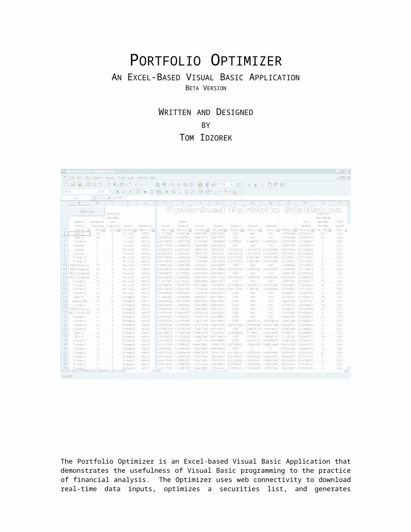
PORTFOLIO OPTIMIZERAN EXCEL-BASED VISUAL BASIC APPLICATION

BETA VERSION

WRITTEN AND DESIGNEDBY

TOM IDZOREK

The Portfolio Optimizer is an Excel-based Visual Basic Application that demonstrates the usefulness of Visual Basic programming to the practice of financial analysis. The Optimizer uses web connectivity to download real-time data inputs, optimizes a securities list, and generates advanced statistics related to individual securities and portfolios. The Optimizer automates mechanical processes that would typically take a financial analyst using Excel many hours to complete.

COPYRIGHT 2002

TABLE OF CONTENTS

OVERVIEW......................................................................................................2

FEATURESGENERAL FEATURES............................................................................2PORTFOLIO STATISTICS........................................................................2INDIVIDUAL SECURITY STATISTICS......................................................3PLANNED FEATURES............................................................................3

DISCLAIMER....................................................................................................3

MAIN MENU...................................................................................................4

OPTIMIZATION SETTINGS................................................................................5

MODIFYING VECTORS....................................................................................6

PORTFOLIO STATISTICS..................................................................................7

STOCK STATISTICS.........................................................................................8

BORDERED PORTFOLIO MATRIX....................................................................9

EFFICIENT FRONTIER....................................................................................10

CORRELATION AND COVARIANCE MATRICES.........................................11-12

INDIVIDUAL ASSET SHEETS..........................................................................13

ACTIVE PORTFOLIO MANAGEMENT STATISTICS..........................................14

APPENDIX A - RUNNING THE OPTIMIZER / TROUBLESHOOTING.............15-17

END NOTES.............................................................................................18-19

PORTFOLIO OPTIMIZER OVERVIEW 1

PORTFOLIO OPTIMIZER

OVERVIEW

The Portfolio Optimizer is an advanced portfolio management tool. In addition to applying the Markowitz paradigm, in which return is maximized for a given level of risk, the Portfolio Optimizer allows the user to select from a number of quantitative asset allocation optimization modes. The Optimizer is a work in progress that incorporates the latest advances in Modern Portfolio Theory, especially optimum portfolio construction / asset allocation models in a user-friendly environment. The Optimizer is a Microsoft Excel-based Visual Basic spreadsheet application; therefore, the numbers are transparent and can easily be manipulated, copied, or linked to other Excel workbooks. The Portfolio Optimizer optimizes entire portfolios or components of portfolios, and enables efficient active portfolio management resulting from fundamental analysis or quantitative screens via optimum tactical asset allocation.

The Optimizer is capable of optimizing portfolios containing up to 249 assets1 - stocks, equity and bond mutual funds, and domestic and international indices. The Optimizer can optimize the constituents of the NASDAQ 100, the DOW 30, the S&P 100, the Major Market Index, the MSCI Developed Markets Index, the MSCI Emerging Markets Index, and the MSCI World Index.

The Optimizer allows the user to create three custom portfolios. Two of the three custom portfolios are designed to be semi-permanent portfolios, entitled Portfolio 1 and Portfolio 2. Once established, Portfolio 1 and Portfolio 2 can be optimized at the touch of a button. The third "Custom Portfolio" uses an input box, which enables the user to quickly clear existing security symbols and input a new list of securities for optimization.2

FEATURES

GENERAL FEATURES

Multiple Optimization Modes: 3 Pure Markowitz Mean-Variance, Treynor-Black, Modified Black-Litterman, or Qian-Gorman Modes

Optimize the MSCI Developed Markets or MSCI Emerging Markets Country Indices Optimize the MSCI All Country World Index Free Download 60+ months of historical price data for each security or index in a portfolio Download 60+ months of historical price data for the benchmark Construct Historic Correlation Matrix Construct Historic, Exponentially-Smoothed, and GARCH-based Covariance Matrices

1 At this time, the theoretical maximum number of assets the Portfolio Optimizer can optimize is 249, due to Excel's limit of 256 columns per worksheet. Large portfolios (100 or more assets) will stress other limits of Excel. Older computers with slower processors and limited RAM will also struggle as the number of assets increases. The downloading of historical data is limited by the speed of the Internet connection. Excel's built-in Solver is also pushed to its limits by larger more complex optimizations. An enhanced Solver is available from the makers of Excel's built-in Solver (http://www.solver.com/). See Page 5, "Optimization Settings," and the corresponding End Notes for additional information on the Portfolio Optimizer's limitations.

2 Once a user becomes familiar with the Portfolio Optimizer, it is easy to cut and paste a list of asset symbols into the appropriate range of cells.


http://www.solver.com/

Build a Bordered Covariance Matrix Calculate Minimum Variance, Equally-Weighted, and Optimum Portfolio statistics Graph the Efficient Frontier and the corresponding Capital Allocation Line Perform Multivariate Portfolio Simulations

PORTFOLIO STATISTICS

Beta of Portfolio Annual Return Annual Standard Deviation Sharpe's Measure Treynor's Measure Jensen's Measure M-squared (Modigliani and Modigliani 1997) Risk-Adjusted Performance (Modigliani and Modigliani 1997) Parametric Value-At-Risk Active Portfolio Management Statistics (Grinold and Kahn 1999)


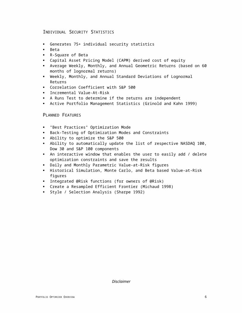
INDIVIDUAL SECURITY STATISTICS

Generates 75+ individual security statistics Beta R-Square of Beta Capital Asset Pricing Model (CAPM) derived cost of equity Average Weekly, Monthly, and Annual Geometric Returns (based on 60 months of lognormal

returns) Weekly, Monthly, and Annual Standard Deviations of Lognormal Returns Correlation Coefficient with S&P 500 Incremental Value-At-Risk A Runs Test to determine if the returns are independent Active Portfolio Management Statistics (Grinold and Kahn 1999)

PLANNED FEATURES

"Best Practices" Optimization Mode Back-Testing of Optimization Modes and Constraints Ability to optimize the S&P 500 Ability to automatically update the list of respective NASDAQ 100, Dow 30 and S&P 100

components An interactive window that enables the user to easily add / delete optimization constraints and

save the results Daily and Monthly Parametric Value-at-Risk figures Historical Simulation, Monte Carlo, and Beta based Value-at-Risk figures Integrated @Risk functions (for owners of @Risk) Create a Resampled Efficient Frontier (Michaud 1998) Style / Selection Analysis (Sharpe 1992)

Disclaimer

Every effort has been made to insure the accuracy of the Portfolio Optimizer; however, the large number of variables (including, but not limited to, different operating systems, versions of Excel and Excel add-ins, hardware / software compatibility, the temperamental nature and complexity of Visual Basic for Applications, complex formulas, and varying sources of current and historical data) may result in errors. No claims regarding the accuracy of the Optimizer are made. Use the Optimizer at your own risk. Any decisions made using the Optimizer are the sole responsibility of the user.

The Optimizer uses data that is available on the Internet. "Terms of Use" change frequently and it is the user's responsibility to comply with the respective Terms of Use of MSCIdata.com, MSN. com, Yahoo.com, PCQuote.com and DBCdata.com.


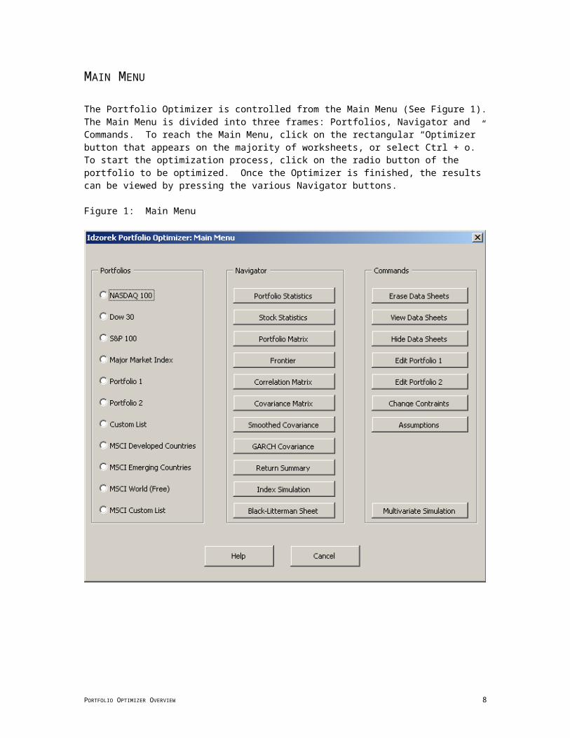
MAIN MENU

The Portfolio Optimizer is controlled from the Main Menu (See Figure 1). The Main Menu is divided into three frames: Portfolios, Navigator and Commands. To reach the Main Menu, click on the rectangular “Optimizer” button that appears on the majority of worksheets, or select Ctrl + o. To start the optimization process, click on the radio button of the portfolio to be optimized. Once the Optimizer is finished, the results can be viewed by pressing the various Navigator buttons.

Figure 1: Main Menu


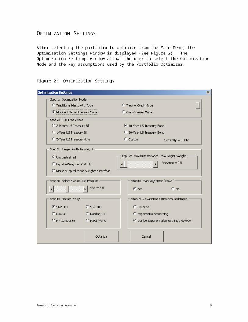
OPTIMIZATION SETTINGS

After selecting the portfolio to optimize from the Main Menu, the Optimization Settings window is displayed (See Figure 2). The Optimization Settings window allows the user to select the Optimization Mode and the key assumptions used by the Portfolio Optimizer.

Figure 2: Optimization Settings


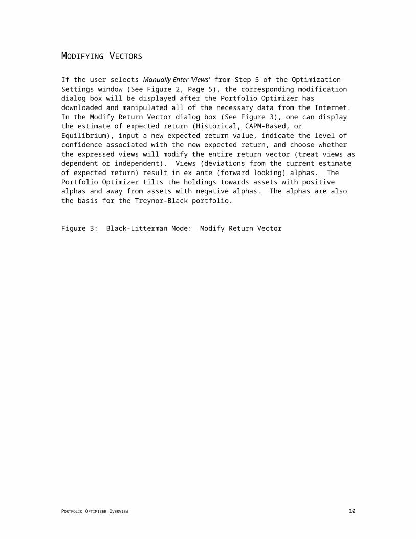
MODIFYING VECTORS

If the user selects Manually Enter 'Views' from Step 5 of the Optimization Settings window (See Figure 2, Page 5), the corresponding modification dialog box will be displayed after the Portfolio Optimizer has downloaded and manipulated all of the necessary data from the Internet. In the Modify Return Vector dialog box (See Figure 3), one can display the estimate of expected return (Historical, CAPM-Based, or Equilibrium), input a new expected return value, indicate the level of confidence associated with the new expected return, and choose whether the expressed views will modify the entire return vector (treat views as dependent or independent). Views (deviations from the current estimate of expected return) result in ex ante (forward looking) alphas. The Portfolio Optimizer tilts the holdings towards assets with positive alphas and away from assets with negative alphas. The alphas are also the basis for the Treynor-Black portfolio.

Figure 3: Black-Litterman Mode: Modify Return Vector


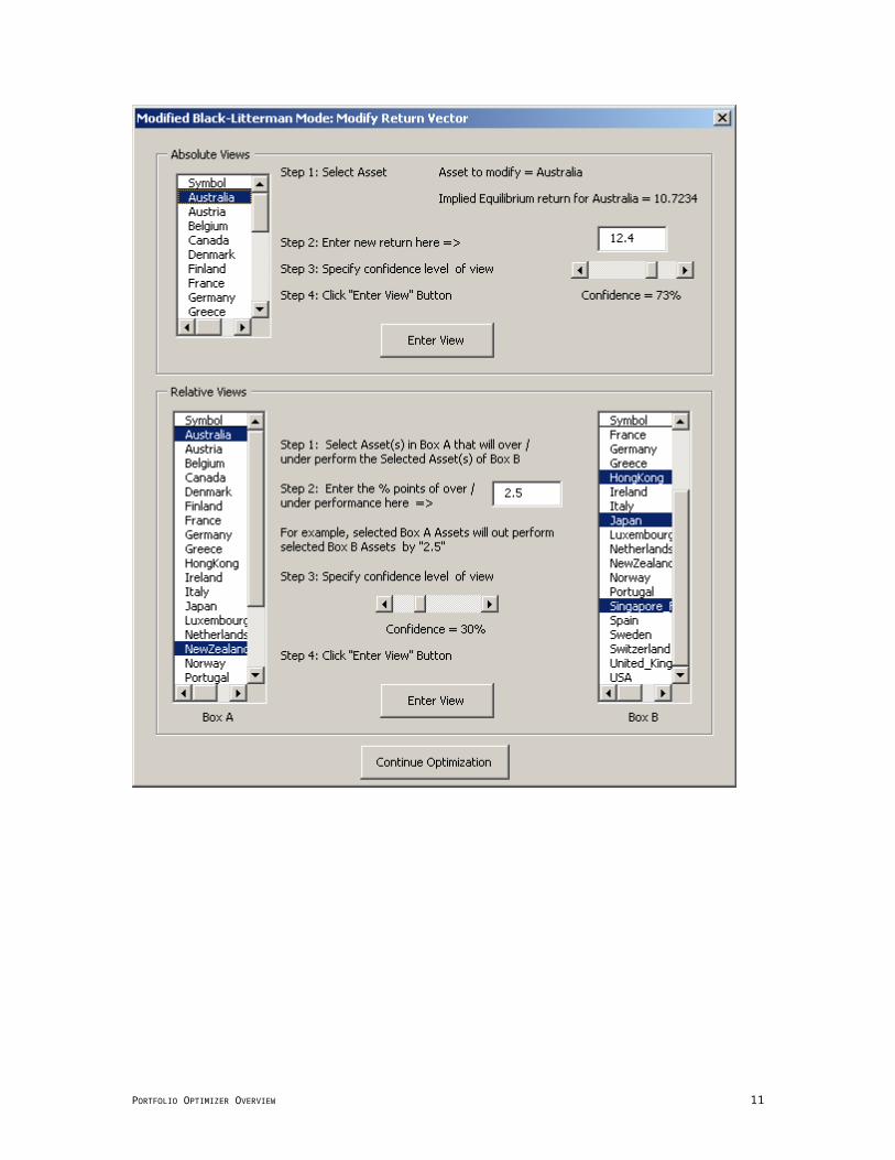
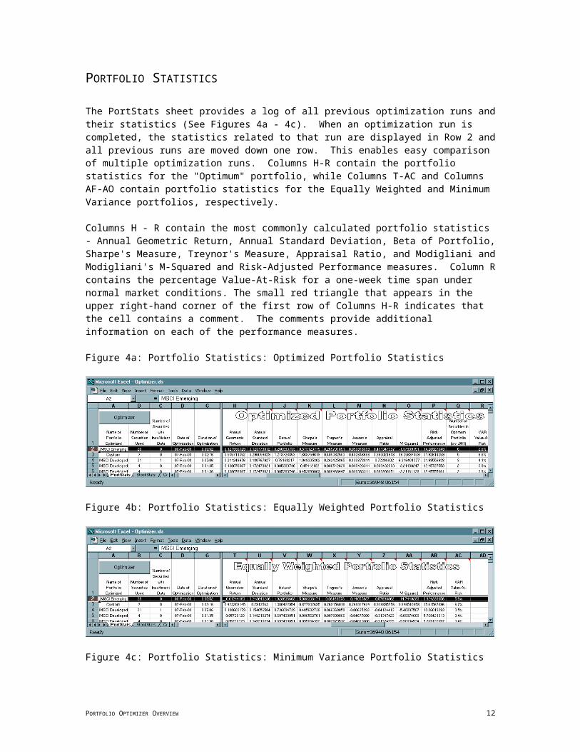
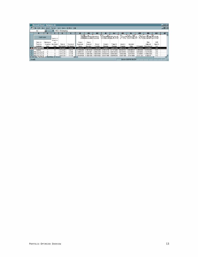
PORTFOLIO STATISTICS

The PortStats sheet provides a log of all previous optimization runs and their statistics (See Figures 4a - 4c). When an optimization run is completed, the statistics related to that run are displayed in Row 2 and all previous runs are moved down one row. This enables easy comparison of multiple optimization runs. Columns H-R contain the portfolio statistics for the "Optimum" portfolio, while Columns T-AC and Columns AF-AO contain portfolio statistics for the Equally Weighted and Minimum Variance portfolios, respectively.

Columns H - R contain the most commonly calculated portfolio statistics - Annual Geometric Return, Annual Standard Deviation, Beta of Portfolio, Sharpe's Measure, Treynor's Measure, Appraisal Ratio, and Modigliani and Modigliani's M-Squared and Risk-Adjusted Performance measures. Column R contains the percentage Value-At-Risk for a one-week time span under normal market conditions. The small red triangle that appears in the upper right-hand corner of the first row of Columns H-R indicates that the cell contains a comment. The comments provide additional information on each of the performance measures.

Figure 4a: Portfolio Statistics: Optimized Portfolio Statistics

Figure 4b: Portfolio Statistics: Equally Weighted Portfolio Statistics

Figure 4c: Portfolio Statistics: Minimum Variance Portfolio Statistics


STOCK STATISTICS

The StockStats sheet provides statistics related to the individual component parts of the portfolio. For each security or country index in the portfolio, the Optimizer downloads historical price information into a new worksheet (See Figure 11, Page 13). The information is then manipulated and security statistics are transferred to the StockStats sheet. The Optimizer displays the Symbol or Index; Portfolio Weight; Beta; R-Square of Beta; CAPM; Weekly, Monthly, and Annual Geometric Returns; Weekly, Monthly, and Annual Standard Deviations; the Correlation Coefficient with the Benchmark; the Incremental Value-At-Risk (in percentage terms and dollar terms based on a $1,000,000 portfolio) that the security contributes to the overall Value-At-Risk, and the results of a Runs Test for randomness conducted on each series of returns. The Portfolio Optimizer generates over 75 statistics for most individual assets.

Figure 5: Stock Statistics


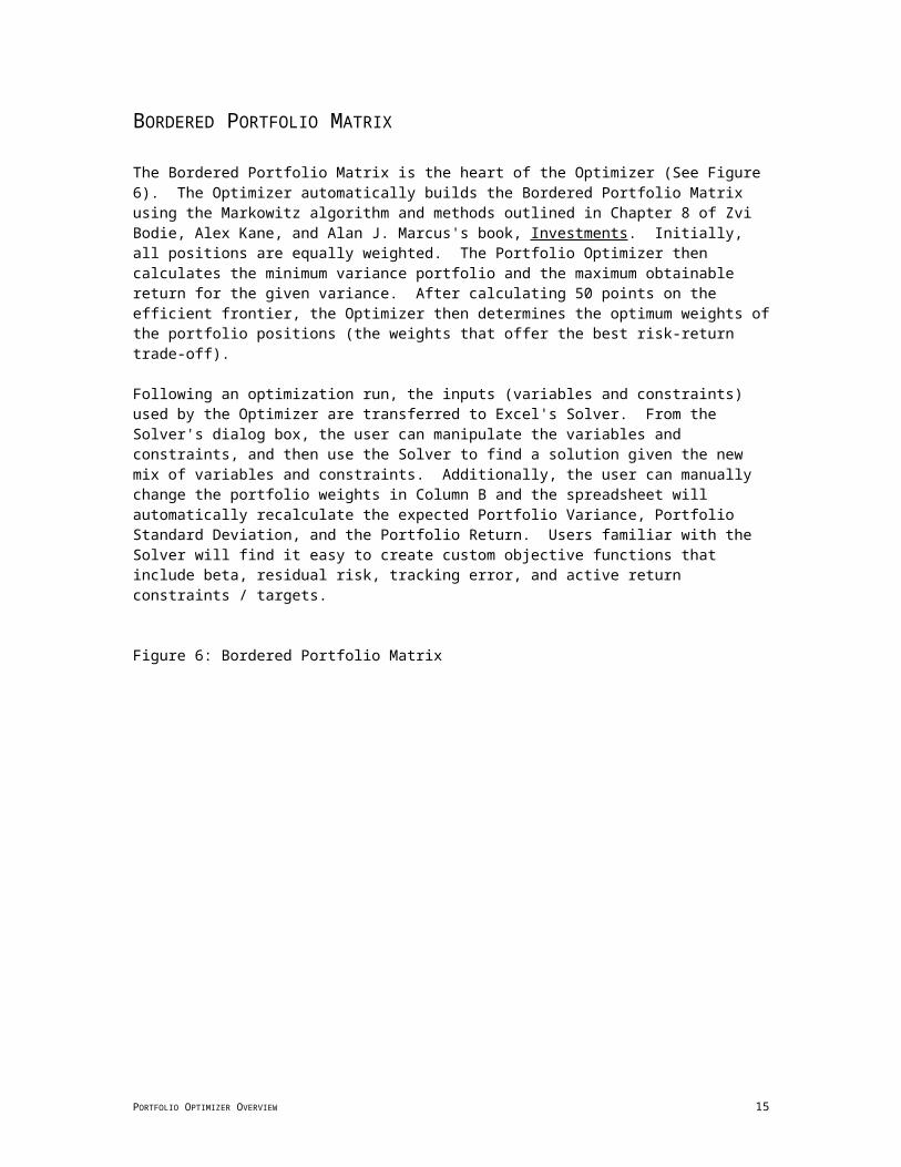
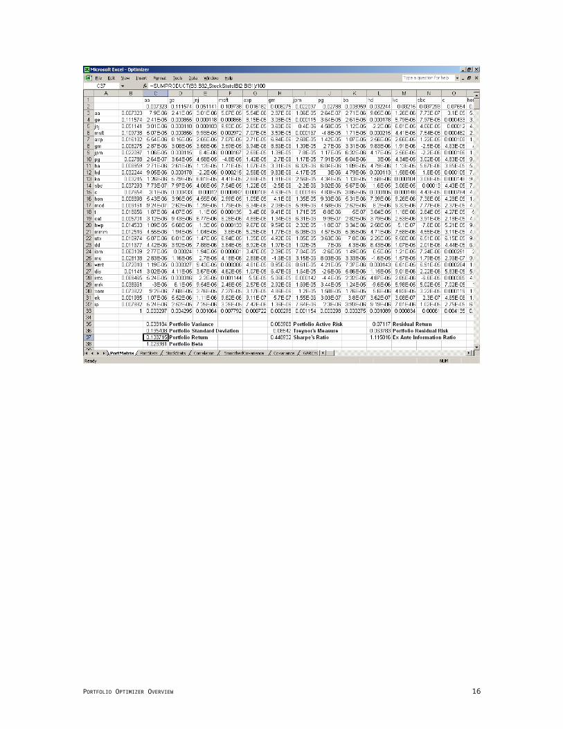
BORDERED PORTFOLIO MATRIX

The Bordered Portfolio Matrix is the heart of the Optimizer (See Figure 6). The Optimizer automatically builds the Bordered Portfolio Matrix using the Markowitz algorithm and methods outlined in Chapter 8 of Zvi Bodie, Alex Kane, and Alan J. Marcus's book, Investments. Initially, all positions are equally weighted. The Portfolio Optimizer then calculates the minimum variance portfolio and the maximum obtainable return for the given variance. After calculating 50 points on the efficient frontier, the Optimizer then determines the optimum weights of the portfolio positions (the weights that offer the best risk-return trade-off).

Following an optimization run, the inputs (variables and constraints) used by the Optimizer are transferred to Excel's Solver. From the Solver's dialog box, the user can manipulate the variables and constraints, and then use the Solver to find a solution given the new mix of variables and constraints. Additionally, the user can manually change the portfolio weights in Column B and the spreadsheet will automatically recalculate the expected Portfolio Variance, Portfolio Standard Deviation, and the Portfolio Return. Users familiar with the Solver will find it easy to create custom objective functions that include beta, residual risk, tracking error, and active return constraints / targets.

Figure 6: Bordered Portfolio Matrix


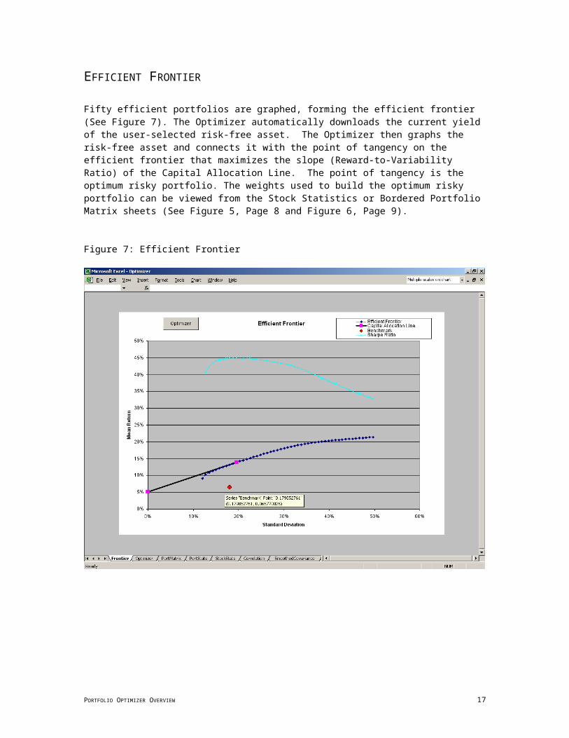
EFFICIENT FRONTIER

Fifty efficient portfolios are graphed, forming the efficient frontier (See Figure 7). The Optimizer automatically downloads the current yield of the user-selected risk-free asset. The Optimizer then graphs the risk-free asset and connects it with the point of tangency on the efficient frontier that maximizes the slope (Reward-to-Variability Ratio) of the Capital Allocation Line. The point of tangency is the optimum risky portfolio. The weights used to build the optimum risky portfolio can be viewed from the Stock Statistics or Bordered Portfolio Matrix sheets (See Figure 5, Page 8 and Figure 6, Page 9).

Figure 7: Efficient Frontier


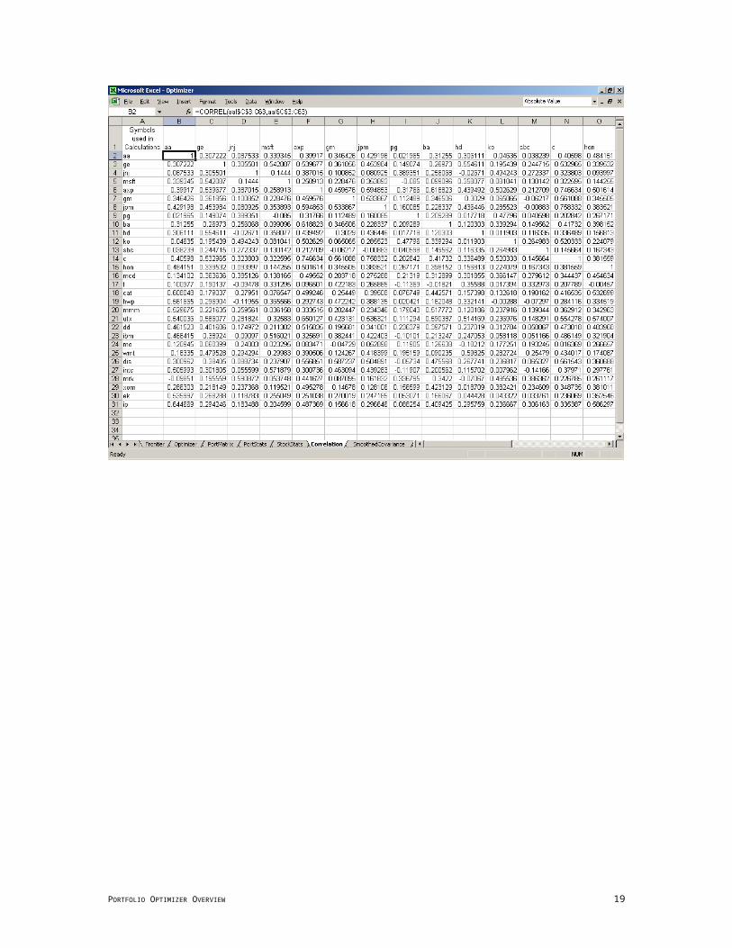
CORRELATION AND COVARIANCE MATRICES

Rather than using a single-index model to estimate correlation and covariance matrices, the Optimizer produces a "full" estimate of correlation and covariance. Using Excel's CORREL and COVAR functions, the correlation coefficient and covariance of each asset pairing is calculated using the most recent 60 months of lognormal returns. Thus, for a portfolio of 100 assets, each matrix includes 4,950 individually estimated relationships.

In addition to these historical-average estimates of correlation (See Figure 8) and covariance (See Figure 9, Page 12), the Optimizer also produces an additional estimate of the covariance matrix using a smoothing average technique common in asset allocation models (See Figure 10, Page 12).4 This exponential smoothing technique recognizes the fact that covariances are not stationary, with more recent observations more accurately depicting the current relationship. Therefore, a weighted-average approach is used, with the greatest weight assigned to the most recent observation and gradually declining weights assigned to the remaining observations.

Finally, the Optimizer is capable of combining an exponentially smoothed estimate of correlation with a generalized autoregressive conditional heteroscedastic (GARCH) model of variance to produce a third estimate of covariance.

The choice of covariance matrix estimation technique is controlled from the Optimization Settings dialog box - Step 7: Covariance Estimation Technique (See Figure 2, Page 5).

Figure 8: Historical Correlation Matrix

4 The Exponentially Smoothed Covariance estimation method is limited to portfolios of 73 or fewer assets. Larger portfolios exceed Excel's matrix math capabilities.

I have used the procedure outlined by Dr. Guillermo Gallego. Dr. Gallego's notes (Lecture #4) and companion Excel file (Smoothing Covariance) are available at http://www.ieor.columbia.edu/~ggallego/4706-00/4706-00.html For a more complete discussion of covariance estimation techniques see Robert Litterman and Kurt Winkelman, “Estimating Covariance Matrices,” Goldman Sachs & Co., Risk Management Series, January 1998.


http://www.ieor.columbia.edu/~ggallego/4706-00/4706-00.html

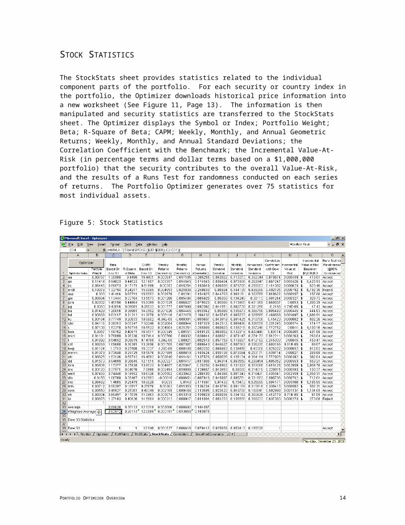
Figure 9: Historical Covariance Matrix

Figure 10: Exponentially Smoothed Covariance Matrix


INDIVIDUAL ASSET SHEETS

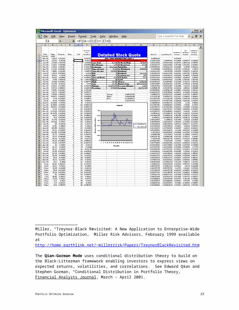
Although they are typically "hidden," an individual worksheet named after the asset is created for each asset in the portfolio (See Figure 11). Each asset's worksheet receives the downloaded data for that particular asset. Unnecessary data is deleted and the remaining data is formatted and manipulated in accordance with the Optimization Settings (See Figure 2, Page 5) for that particular optimization run. A “Runs Test for Randomness” is conducted in Columns D and E. A “Detailed Stock Quote” is downloaded from PCQuote.com and inserted in to the worksheet. Columns N – R contain a generalized autoregressive conditional heteroscedastic (GARCH) model of variance.5 The values that maximize the likelihood function of the GARCH model are in Rows 20 – 23 of Columns K and L.

Figure 11: Individual Asset Worksheet for AOL Time Warner Inc.


ACTIVE PORTFOLIO MANAGEMENT STATISTICS

The Portfolio Optimizer generates Active Portfolio Management Statistics, as described by Richard Grinold and Ronald Kahn in their book, Active Portfolio Management. Active Portfolio Management Statistics are calculated for individual assets as well as entire portfolios. Statistics related to individual assets, which may in fact be portfolios of individual assets (such as mutual funds or indices), are located in Columns BP - BZ of the StockStats worksheet (See Figure 12). Corresponding Active Portfolio Management Statistics for the entire portfolio of optimized assets are located in Columns BD-BK of the PortStats worksheet.

Figure 12: Active Portfolio Management Statistics


APPENDIX A - RUNNING THE OPTIMIZER / TROUBLESHOOTING

RUNNING THE OPTIMIZER

Step 1: Saving the Optimizer – Save the Optimizer.xls file to the hard drive (Do not rename the file).

Step 2: Enable Macros – When the Optimizer.xls file is opened, a warning message similar to the one below will appear. To run the Portfolio Optimizer, you must select ENABLE MACROS.

Step 3: Main Menu – After selecting “Enable Macros,” the screen should resemble the one below. Select Continue and then Select the Optimizer Main Menu button or Ctrl + “o” Depending on the computer’s display settings, one may need to scroll down to see the Optimizer Main Menu button.


INSTALLATION / TROUBLESHOOTING

If Step 1 - Step 3 did not occur as described, settings and / or add-in components may need to be altered. The Portfolio Optimizer uses Excel's most advanced features; thus, a “full” version of Excel, including many of its add-ins must be properly installed. If Excel or its add-ins are not properly installed, or a component of Excel is corrupt, a "compile error" is likely.

Step 4: Security Settings – In order to run macros, Excel security settings may need to be lowered. From the Tools menu, select Options, and then Security. On the Security Tab, select Macro Security and then reduce the security setting to Medium or Low.

Step 5: Add-Ins – To install the add-ins, select “Add-Ins” from the "Tools" menu. The following boxes, with the exception of the “Euro Currency Tools,” must be checked:

The checking of additional “Add-Ins” should not present a problem. It is a good idea to restart the computer after installing the add-ins. Once the Portfolio Optimizer is open, select “Add-ins” from the “Tools” menu again and confirm that the appropriate boxes are checked. The Portfolio Optimizer should now run without errors.

Step 6: Break On All Errors – Start the Visual Basic Editor (press ALT+F11). From the Options dialog box (General tab) in the Visual Basic Editor, deactivate Break on All Errors option.

Step 7: Solver Reference – If errors continue to occur, complete three more steps:

a) In Microsoft Excel, start the Visual Basic Editor (press ALT+F11).

b) On the Tools menu, click References.

c) Select the Solver check box, and then click OK. (One may need to “Browse” to the Solver’s location.)

97 and 2000: The Solver.xla file is located in C:\Program Files\Microsoft Office\Office\Library\Solver.XP: The Solver.xla file is located in C:\Program Files\Microsoft Office\Office10\Library\Solver


Step 8: Multiple Versions of Excel – It is best to have only one version of Excel installed.


TROUBLESHOOTING SPECIFIC ERROR MESSAGES

OFFICE XP

ERROR MESSAGE:

3 The Traditional Markowitz Mode uses historical returns to forecast expected returns. See Zvi Bodie, Alex Kane, and Alan J. Marcus, Investments Fourth Edition, Chapter 8. See also Harry Markowitz, "Portfolio Selection," Journal of Finance, March 1952.

The Black-Litterman approach, created by Fischer Black and Robert Litterman of Goldman Sachs, is a sophisticated Baysian method used to overcome the problem of unintuitive, highly-concentrated, input-sensitive portfolios. Rather than using historical returns to forecast expected returns (the input used by the traditional Markowitz Mean-Variance method), the Black-Litterman Model uses "equilibrium" returns as a neutral starting point. Equilibrium returns are calculated using the CAPM (an equilibrium pricing model) or by a reverse optimization method in which the vector of expected equilibrium returns (Π) is extracted from known information. Using matrix algebra, one solves for Π in the formula, Π = δ Σ weq, where weq is the market capitalization weights; Σ is a fixed covariance matrix; and, δ is a risk-aversion coefficient. If the portfolio is "well-diversified," this method of extracting the implied expected equilibrium excess returns produces an expected excess return vector very similar to the one generated by the Sharpe-Littner CAPM. CAPM-generated estimates of expected returns have a tight range compared to expected returns based on historical returns. As a result, optimizations based on CAPM expected returns distribute portfolio weights over a far greater number of assets. The implied equilibrium expected excess returns coupled with the fixed covariance matrix and the risk-aversion coefficient lead back to the market capitalization weighted portfolio - the market (benchmark) portfolio. Using conditional probability theory, the Black-Litterman Model combines the implied equilibrium expected excess returns with individually expressed views to produce a new conditional expected excess return vector. A view thus alters the entire vector of expected excess returns in such a way that only the weights of the assets in which a view was expressed will deviate from their equilibrium market capitalization weights. This has the effect of constraining the assets in which a "view" was not expressed. Depending upon the selections made by the user, while in Black-Litterman Mode, the Portfolio Optimizer will use either the CAPM expected returns or the implied equilibrium expected returns. The implied equilibrium returns of the components of the index should equal the CAPM-based estimates of expected returns when that particular index is used to estimate the CAPM estimate of expected returns. However, this is the exception because many of the indices undergo changes to their components during the relative time period. Therefore, the Portfolio Optimizer creates a simulated market index based on historical price data and market capitalization weights for a given input list. The simulated market index is used to create an alternative forecast of CAPM expected returns. The “true” Black-Litterman model is used for portfolios of 73 and fewer assets. Portfolios with more than 73 assets exceed Excel’s matrix capabilities; thus, a Modified Black-Litterman mode is used that relatively accurately applies the Black-Litterman approach to larger portfolios. See Fischer Black and Robert Litterman, “Global Portfolio Optimization,” Financial Analysts Journal, September - October 1992, 28-43. See also Guangliang He and Robert Litterman, “The Intuition Behind Black-Litterman Model Portfolios,” Goldman, Sachs & Co., Investment Management Research, December 1999. See also Wai Lee, “Chapter 7: Black-Litterman Approach,” Advanced Theory and Methodology of Tactical Asset Allocation, Fabozzi & Associates, 2000. Thomas Idzorek, “A Step-By-Step Guide to the Black-Litterman Model,” Working Paper.

The Treynor-Black Mode, like the Black-Litterman Mode, assumes that the market is nearly efficient, but also allows the active portfolio manager the opportunity to express views regarding mispriced assets. Based on the expressed views that lead to positive or negative alphas relative to the current estimate of expected return, the Optimizer constructs the optimum "active" portfolio and determines what portion of PORTFOLIO OPTIMIZER OVERVIEW 20

SOLUTION:

1. From the “Tools” Menu, select “Solver.”2. Select “Solve” from the following dialog box.

3. Select “OK.”

the total portfolio to allocate to the active and passive portions of the portfolio. Treynor-Black Statistics are located in Columns CB - CK of the StockStats worksheet. See Zvi Bodie, Alex Kane, and Alan J. Marcus, Investments Fourth Edition, pages 876 - 883. See also Jack Treynor and Fischer Black, “How to Use Security Analysis to Improve Portfolio Selection,” Journal of Business, January 1973 or Ross M. Miller, “Treynor-Black Revisited: A New Application to Enterprise-Wide Portfolio Optimization,” Miller Risk Advisors, February 1999 available at http://home.earthlink.net/~millerrisk/Papers/TreynorBlackRevisited.htm

The Qian-Gorman Mode uses conditional distribution theory to build on the Black-Litterman framework enabling investors to express views on expected returns, volatilities, and correlations. See Edward Qian and Stephen Gorman, “Conditional Distribution in Portfolio Theory,” Financial Analysts Journal, March - April 2001.

5 The GARCH model is based on an Excel spreadsheet model created by Stephen Gray. Rather strict parameters (constraints) are used in the automation of the model to increases its stability. The original Excel file, and a wealth of great information, is available at Campbell R. Harvey’s Global Asset Management and Stock Selection course page (http://www.duke.edu/~charvey/Classes/ba453/syl453.htm).


http://www.duke.edu/~charvey/Classes/ba453/syl453.htm

http://home.earthlink.net/~millerrisk/Papers/TreynorBlackRevisited.htm

4. Select “Close” from the “Solver Parameters” dialog box, which will reappear after selecting “OK” from Step 3.

5. Select Ctrl + “o” to re-start the Optimizer.


END NOTES


tom idzorek’s portfolio optimizer - fuqua school of …charvey/teaching/ba453... · web...

Documents