top incomes in chile using 50 years of household … · top incomes in chile… / claudia sanhueza,...

Top incomes in Chile… / Claudia Sanhueza, Ricardo Mayer 169Estudios de Economía. Vol. 38 - Nº 1, Junio 2011. Págs. 169-193

* We thank Sergio Ríos for his excellent research assistance.** Instituto de Políticas Públicas, Universidad Diego Portales, Ejército 260, Santiago, Chile.

E-mail: [email protected].*** Facultad de Economía y Empresa, Universidad Diego Portales, Manuel Rodríguez Sur 0253,

Santiago, Chile. E-mail: [email protected].

Top Incomes in Chile using 50 years of household surveys: 1957-2007*Ingresos más altos en Chile usando 50 años de encuestas de hogares: 1957-2007

Claudia Sanhueza**Ricardo Mayer***

Abstract

Using household surveys that cover more than 50 years of the political and economic history of Chile, we investigate changes in the shape of the distribution of income in Chile, and in the composition of top 10% and top 1% incomes. In line with international evidence, top incomes concentration appears to be countercyclical in the short run. For the entire length of this survey, this con-centration shows roughly an inverted U-shape, peaking at the end of the 80s. These changes correspond approximately with different economic policy regimes prevailing in Chile. We observe important changes in the composition of top income groups related to greater relative importance of women, employees and college schooling levels. These changes are stronger for the top 10% than the top 1% of incomes. Additionally, using a national level panel of households for the period 1996-2006 we explore correlations between probabilities of perma-nence and arrival to the top decile with variables such as composition of the household, ownership of physical and human assets, job quality and changes in the numbers of household members working in the labor market.

Key words: Income distribution, Income mobility.

Resumen

Usando encuestas de hogares que cubren más de 50 años de la historia política y económica de Chile, investigamos los cambios en la forma de la distribución del ingreso en Chile y en la composición del 10% y 1% superior. De acuerdo con la evidencia internacional, la concentración de los ingresos más altos parece ser contracíclica en el corto plazo. Para todo el período de estudio,

Estudios de Economía, Vol. 38 - Nº 1170

esta concentración muestra una forma de U invertida, alcanzando un máximo a finales de los años 80. Estos cambios corresponden a diferentes regímenes de política económica vigentes en Chile. Observamos cambios importantes en la composición de los grupos de ingresos más altos: mayor importancia relativa de mujeres, empleados y personas con educación universitaria. Estos cambios son más fuertes para el 10% que para el 1% más rico. Además, utilizando un panel nacional de hogares para el período 1996-2006 se exploran las correlaciones entre las probabilidades de permanencia y llegada al decil 10 con variables tales como la composición de la familia, la propiedad de activos físicos y humanos, la calidad del empleo y los cambios en el número de miembros del hogar que trabajan en el mercado de trabajo.

Palabras clave: Distribución del ingreso, Movilidad del ingreso.

JEL Classification: D31, J6.

1. Introduction

An income distribution more concentrated at the top has significant implica-tions for the economy and politics. Leigh (2009) argues that if a small elite gets a big share of society’s income, it could influence certain industries and, through their campaign contributions, certain politicians. Moreover, Frank (2007) notes that the increase in spending of high-income individuals can affect the middle class because of a contagion effect on the rest of the population. He argues that the welfare evaluation depends on context, and therefore consumption choices also depend on the comparison made by the individual with respect to those around him. Finally, Tawney (1913) argues that understanding the concentra-tion of incomes at the top of distribution tells us something about the bottom part of it, since the concentration of income at the top is highly correlated with relative poverty.

With this in mind, several authors have analyzed the evolution of top incomes by building long time series of top income shares during the twentieth century. This includes Piketty (2003), Piketty and Saez (2006), Atkinson (2002), Saez and Veall (2005), Atkinson and Leigh (2005, 2007), Atkinson and Piketty (2007), Atkinson and Salverda (2005), Banerjee and Piketty (2005) among others. On the other hand, Saez and Veall (2005) and Kopczuk, Saez and Song (2007) have also studied the welfare consequences of income mobility at the top of the income distribution and the effect of the increase in female labor participation.

These topics are especially important in Latin American countries, given that most of them present the world’s worst indicators of income inequality and the factors behind this high and stable inequality are in permanent discussion. Chile, the subject of this paper, ranks among the most unequal countries in the region,1 only bellow Brazil, Guatemala and Colombia.

1 World Bank Report, 2003, “Inequality in Latin America: Breaking with History?”, Chapter 1.

Top incomes in Chile… / Claudia Sanhueza, Ricardo Mayer 171

During the last 50 years Chile has faced various types of economic situa-tions as a result of international events or policies developed within the country. Including conservator, social-democratic and socialist governments and a 17 years strong dictatorship. In the last two decades, after the dictatorship, Chile has shown high growth rates, greater macroeconomic stability, significant reduction in poverty rates, all generating well-being of the population. However, with all this progress the issue of income inequality shows no improvement, and Chile is among the countries with the highest levels of inequality in Latin America. The richest 10 percent of individuals in Chile receive 47 percent of total income and the bottom 20 percent receive 3.4 percent. By way of comparison, in the United States the richest 10 percent receive 31 percent of total income, and the bottom 20 percent receive 5.2 percent of the total income.

The evolution of income inequality has attracted the attention of both economic and political studies, especially as the economy grows. This evolution has been affected by different changes: developments in technology, policy interventions, political shocks, changes in social indicators and other factors. Although, Chile has grown there is the doubt about whether this has led to benefit a small group or owners of the capital, leaving behind a large group of the population.

Studies done for Chile show that in the short term, the distribution of income does not appear to be affected, so that one can sense that specific policies do not have permanent or long term consequences and therefore they will not be effective to combat the problem of income inequality. Thus, the analysis is to be returned to a long-term horizon, and that is why it is necessary to have historical series, which allows us to understand the problem.

The aim of this paper is to study the evolution of top income shares in Chile and the composition of this group during the last 50 years. In addition, using panel data we study income mobility at the top of the distribution in recent years and its determinants. The available information allows us to study the evolution of top incomes shares, distinguishing between individual and family income, and hence to investigate if the increase of female participation rate in the labor market has contributed to greater income concentration due to the interrelation between spouses’ income.

To study the evolution of top incomes in the last 50 years we use the Employment and Unemployment Survey of the University of Chile. This survey contains considerable information about incomes for a sample of households in Greater Santiago between 1957 even today. With this information the following indicators are constructed: average real income of decile 10, percentile 1, per-centiles 10 to 2, growth of those average incomes, participation relative to the entire revenue of every year, distances between average income and decile 10’s average income and others. All these indicators are constructed for both household and individual incomes. Additionally, we analyze their composition in terms of wages and other incomes, education, gender and types of occupation.

In turn, for the analysis of mobility in decile 10, we use CASEN panel surveys. This allows us to study transitions in the upper part of the distribution, answer-ing the question of what is the probability of remaining in decile 10 and the probability of arriving to the top decile 10. Moreover, the wealth of information readily available in household surveys allows us to study the variables correlated with the probability of remaining in decile 10 and of arrival to decile 10, using initial conditions as explanatory variables, including household composition variables, household assets and shocks.


This paper contributes to the debate on the income distribution in Chile in several ways. First, to our knowledge this is the first time that the long series of top incomes has been analyzed for the Chilean case, which is key to getting insights about the effects of different economic policy regimes. Ruiz-Tagle (1998) uses the same survey to build indicators of income distribution over 40 years, however, he did not analyze what happened to the top income shares. Second, the determinants of the probability of arriving and remaining at the top of the income distribution have not been analyzed before. Contreras et al. (2004) study the dynamic of poverty using one of the waves of Panel Casen surveys. They do not include the study of the dynamic of the top of the distribution.

It is worth noting that we use survey data rather than income tax data. Most of top income studies have made use of tax data. Saez (2004) argues that sur-veys information is available only in the recent years and that, at least in the United States, the household surveys present information on codified form or by stretches. On the other hand, tax data also suffer from certain problems. First of all, income information is based on self-reported information therefore problems of evasion and elusion can slant the results. Second, taxes statistics cover only a fraction of the population. Historically, the fraction of the population who declares income is small and there is a big part that is exempt of it or where informality conditions prevail in the labor market. These facts are especially important in the case of Chile.

For this research, we maintain that the use of household surveys allows us to address these issues. First, the extraordinary series of 50 years of the Employment and Unemployment Survey allows us to circumvent the issue of short lengths of time. Second, income data is captured as a continuous variable, and not coded into income sections. Also the information in the survey registers the identity of income sources and whether they are individual or family figures. Third, household incomes in the surveys may come from informal mechanisms or be exempt from taxes.

The structure of the papers is as follows. After this introduction we present a brief literature review. Then we present the data and methodology in section 3. In section 4 we present the evolution of top incomes in Chile and in section 5 the mobility analysis at the top of the income distribution. Finally, section 6 concludes.

2. Literature Review

A review of recent literature is available in Saez (2004), Piketty and Saez (2006) and Leigh (2009). Series of top incomes have been produced for various developed countries, including Australia (Atkinson and Leigh, 2007), Canada (Saez and Veall, 2005), Finland (Riihelä, Sullström and Tuomala, 2005), France (Piketty, 2003), Germany (Dell, 2007), Ireland (Nolan, 2007), Japan (Moriguchi and Saez, 2008), Holland (Atkinson and Salverda, 2005), New Zealand (Atkinson and Leigh, 2005), Spain (Alvaredo and Saez, 2006) Switzerland (Dell 2005, Dell, Piketty and Saez, 2007), United Kingdom (Atkinson, 2002, 2007) and U.S. (Piketty and Saez, 2003).

Piketty (2004) and Legih (2009) emphasize that international comparisons find a significant decrease in top income share during the first half of the twentieth


century in all countries except Switzerland, with a later increase of this shares in the second part of the century mainly in Anglo-Saxon countries but not in Japan and continental Europe. Indeed, top income shares make a full recovery in the U.S., a significant one in England and Canada, and none in France. This fall in the first part is attributed to the incorporation of highly progressive tax systems after the Second World War and the subsequent growing importance of salaries in the composition of top incomes, which in turn have won profitability due to technological progress. Moreover, Leigh (2009) noted that differences between countries are not due to institutional differences in the labor market, such as levels of centralization of collective bargaining.

Atkinson (2002) studies the evolution of top incomes in the United Kingdom. In his research advances beyond what previous authors had developed for the UK since it tries to identify the amount of aggregate income and aggregate popula-tion and argues that his data is a unique source of evidence on the distribution of higher incomes which allows him to cover the twentieth century. He shows that the First and Second World Wars conveyed a significant drop in the income shares of the top 0.05% and 1% incomes. Piketty (2003), in turn, studies the same series for France. In particular, he concludes that the decline in France of income inequality is largely accidental.

For the United States, Piketty and Saez (2003) work with a database with information about the concentration of wealth and income. They acknowledge that working with this type of information has important limitations. In particular they mention that their long term series have little information on the bottom incomes, but because of being homogeneous across the countries and decom-posed in different income sources, they are the only opportunity to understand the dynamics of the distributions of income and wealth. They mention that the general pattern, across the century, for decil 10’s income has a U shape, that it experienced a substantial decrease, greater than 30% during WWII, and that remained above 31 and 32 per cent until 1970. After decades of stability in the post-war period, the share of the richest decile increased dramatically on the last 25 years, reaching its pre-War levels, but with a different composition in which the labor income is now the main income source.

Additionally, Saez and Veall (2005) studied the evolution of high-income families and individuals, concluding that the historical evolution of both series follow the same pattern. This indicates that in spite of increasing incorpora-tion of women into the labor market, this does not improve or deteriorate the concentration of incomes, probably due to the correlation between the earnings of spouses. They also study the consequences in terms of welfare for income mobility. They find that there has been an increase in mobility in Canada at the top of the income distribution.

In each of the works mentioned the methodology is very similar, and so are the main conclusions, apparently because developed countries have followed the same trend in the implementation of tax policies. For example, Piketty (2003) argues that many authors have said that the dramatic increase in progressive taxation taking place in the interwar period has been the main factor that prevent income and wealth shares return to their previously high levels. This taxation trend would explain also the generally observed decrease in the relative importance of capital revenues and an increase in the relative importance of labor income as determinant of total income, at least in recent decades.


A short background about Chile

Chile has been pointed out as an example of successful economic development among developing economics. During the last decades has shown an increas-ing and currently high per capita GDP, a significant reduction in poverty rate and economic and political stability. A set of innovative reforms implemented during the last decades have made of Chile a reference for countries in similar, lower and even upper stages of development. However, and despite the success, probably the single most important failure of the Chilean experience has been the high and apparently permanent income inequality.

Ruiz-Tagle (1998) uses the Employment and Unemployment Survey of the University of Chile and constructs series of indicators of income distribution in Santiago (Chile). He concludes that inequality has generally increased since 1957, peaking during the 1980’s and improving a little over the following decade. The indicators he uses exhibit high levels of persistence over time, leading him to conclude that income distribution cannot be modified significantly over short periods of time. Larrañaga (1999) studies the relationship between economic growth and income distribution in Chile in the 1987-1996 period. To this end, he uses CASEN household surveys from years 1987, 1990, 1992, 1994 and 1996, disaggregating the dynamics of growth and income distribution in a sector-by-sector basis. His main findings are an increasing and concave relationship between mean income and sector’s inequality, and a positive correlation between mean income and changes in levels of inequality. These two findings hold for short run (two years) as well as for long run (ten years) analyses. Larrañaga and Valenzuela (2011) study the factors behind the stable and high-income inequality in Chile, given the great changes realized in the country from 1990 to 2003. They concluded that although several factors changed over the period their effects over inequality cancelled out. Valenzuela y Duryea (2011) using micro-simulations compare the income distribution of Chile with respect to Uruguay. They find that the main differences between the two countries are present at the top of the distribution, and they are due to the composition of income in those deciles. In Chile the propor-tion of income that comes from employer’s income is higher and more unequal. Finally, Sapelli (2011) looks at the income distribution by cohorts in Chile by constructing a synthetic panel and estimate the income distribution for cohorts born between 1902 and 1978. The cohort effects show a period where inequality increases and then decreases. The rise can be explained by variables associated with education, while the fall appears to be the consequence of a flattening of the income-age profile and hence a reduction in the returns to experience. Engel and Eberhard (2007) show evidence that inequality has been decreasing since 1990s due to a decrease in the college skill-premium that was due to the deregulation of the college market during 1980s.

Regarding short-run mobility analysis Contreras, et al. (2004) analyzes the dynamics of the relationship between poverty and poverty mobility using CASEN panel survey for 1996 and 2001. They look at probabilities of arriving to and departing from poverty and the factors behind these movements in and out of poverty. They find high mobility in all deciles from deciles 1 trough 9, which implies that more than half of the population is potentially in risk of fall-ing into poverty. The opposite holds for the transition between deciles 9 and 10, for which there is no such high mobility. The bottom forty percent of the income


distribution does not have the resources to deal with illness or health hazard affecting the household head. On the other hand, long-term mobility estimates show high-income elasticity and therefore a country with low social mobility (Nuñez and Risco, 2004 and Celhay et al., 2010).

3. Data and Methodology

Regarding the analysis of the evolution of top incomes we use the Employment and Unemployment Survey of the University of Chile. This is the oldest survey available in Chile and has rich relatively information on income of households in Greater Santiago from 1957 up to current date. Another key feature of this database is its homogeneity, as the survey format has remained virtually the same over all these years, therefore information is similar throughout the period, making it easier to validate comparisons over time.

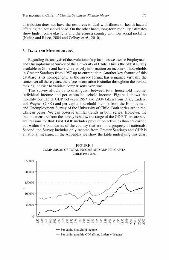
This survey allows us to distinguish between total household income, individual income and per capita household income. Figure 1 shows the monthly per capita GDP between 1957 and 2004 taken from Diaz, Luders, and Wagner (2007) and per capita household income from the Employment and Unemployment Survey of the University of Chile. Both series are in real Chilean pesos. We can observe similar trends in both series. However, the income measure from the survey is below the range of the GDP. There are sev-eral reasons for that. First, GDP includes production activities than are carried out within the boundaries of the country that are not a property of nationals. Second, the Survey includes only income from Greater Santiago and GDP is a national measure. In the Appendix we show the table underlying this chart

FIGURE 1COMPARISON OF TOTAL INCOME AND GDP PER CAPITA:

CHILE 1957-2007

0

50000

100000

150000

200000

250000

$

Per capita household income

Per capita monthly GDP (Diaz, Luders y Wagner)

1957

1967

1969

1971

1973

1975

1977

1981

1985

1983

1987

1989

1991

1993

1995

1997

1999

2001

2003

2005

2007

1979

1959

1961

1963

1965


and also a comparison between individual and total income of the household. Incomes from the survey were corrected by CPI to be left in real Chilean pesos, and moreover, the different currencies used during the period of study were made equivalent. The sample size corresponds, roughly, to 10,000 people and 5,000 households on average per year.

Table 1 shows some descriptive statistics for the year 2007. We focus on the decile 10 and the 99th percentile of income distribution. We see that the average household income was 511,929 Chilean pesos (930 dollars). The median on the other hand, is 338,929 (615 dollars). In the case of income distributions with a long tail, the median is a better indicator of mean income than the average income. Moreover, the average total household income in decile 10 is 1,895,859 Chilean pesos (3,450 dollars), and within the richest 1% is 4,333,647 Chilean pesos (7,880 dollars). The minimum household income of decile 10 is 1,060,429 (1,930 dollars) and the minimum household income of percentile 99 is 3,305,993 (6,010 dollars). This shows the great gap between incomes of the richest deciles and average households in Chile.

TABLE 1AVERAGE INCOME THRESHOLDS AND TOP 10% AND TOP 1%, CHILE, 2007

Average population

MedianAverage top 10%

Average top 1%

p90 p99

Total household income 511,929 338,969 1,895,859 4,333,647 1,060,429 3,305,993 Individual income 246,201 157,767 1,028,191 2,948,340 518,915 1,740,877 Per capita household income 130,713 82,357 315,574 1,254,873 273,407 841,144

Source: Employment and Unemployment Survey, Universidad de Chile, 2007. 8,870 individuals. 4,934 households.

Income proportions were calculated using as a numerator the sum of in-comes of all individuals or households in decile 10 (and top 1 %), divided by the sum of the income of all individuals or households in the sample. Another way of doing it would be to use as denominator the monthly GDP of the coun-try. Nevertheless, as we said previously this one includes incomes that are not a property of nationals. In case of the individual income they include only the income of individuals who work or have personal individual revenue.

On the other hand, the survey has information on the sources of individual income. This allows us to distinguish the differences in the evolution of the dif-ferent sources for top incomes: wages, capital gains or other incomes. Income is divided in the following way: i) salaries and wages, ii) independent income, originated from industrial, agricultural, commercial and professional activities, iii) pensions and iv) other incomes, which includes capital revenues in addition to other non welfare income. We also take other individual information, such as the type of occupation and gender.


To perform mobility analysis in the high part of the income distribution, however, we need longitudinal information. The survey panel that covers the longest time period in Chile is the survey Panel CASEN 1996-2006. Using three periods of the survey we calculate matrices of mobility for the top decile between 1996-2001 and 2001-2006. Also, we estimate two models of discreet dependent variable in which we identify variables correlated with the probability of permanence in the decile 10 from the rest of the distribution and variables correlated with the probability of arrival to the 10th decile.

The permanence in the top decile is studied by means of the construction of a discreet variable that takes the value of 1 if the household is observed in the 10th decile in year t conditional on being in decile 10 in year t–1, and 0 if person is not observed in decile 10 in year t conditional on being in decile 10 in year t–1. The model incorporates characteristics of the household in year t–1, and changes produced between t–1 and t.

For the case of arriving to the decile 10 we generate a discreet variable that take the value of 1 if the household is observed in decile 10 in year t condi-tional on been in decile 10 in year t–1, and 0 if the household is not observed in decile 10 in year t conditional on not been in decile 10 in year t–1. The model incorporates characteristics of the household in year t–1, and changes produced between t–1 and t.

The explanatory variables for both models include composition of the house-hold, physical and human capital, household’s geographic characteristics and shocks. Shocks include health problems, changes of the numbers of persons in the household, and changes of the number of persons in the household that work.

4. Top Incomes Evolution in Chile

Figure 2 shows the evolution of the top decile’s share of total household’s income in Chile between the years 1957 and 2007. Just like the available evidence for other countries has suggested elsewhere, the behavior of this series appears to be countercyclical. During a economic crisis, for example during the crisis of 1982, the population’s elite who enjoy major capital endowment will increase his economic differences with those more disadvantaged. On the other hand, during periods of economic expansion as those that happened from 1987 up to 1996, the participation of decile 10 was diminishing. When the country began to slow down its economic growth, the income share of the rich began rising again. The evidence suggests that for periods of rapid economic growth wage gaps tends to diminish and the opposite holds for periods of slower or negative economic growth. Also we can observe a inverted-U shape for top income shares in the period under study, which reaches a maximum at the end of the 80s.

Figure 3 shows the series of income shares of the household grouped in income ranges p90-95, p95-99 and p99-100. We note that in periods of growth of the top decile ( p90-100) it was primarily due to growth in the richest part of the top decile: p95-99 and p99-100. The indicator for p90-95 percentile even decreases gradually in the period under study. This shows that the concentration in the upper part of the distribution is mainly determined by what happens in the richest 5% of the population.


FIGURE 2PROPORTION OF INCOME DECILE 10

FIGURE 3PROPORTION OF INCOME p90-95, p95-99, p99-100

20.00

25.00

30.00

35.00

40.00

45.00

50.0019

5719

5919

6119

6319

6519

6719

6919

7119

7319

7519

7719

7919

8119

8319

8519

8719

8919

9119

9319

9519

9719

9920

0120

0320

0520

07

%

Decile 10

0.00

5.00

10.00

15.00

20.00

25.00

30.00

1955

1957

1959

1961

1963

1965

1967

1969

1971

1973

1975

1977

1979

1981

1983

1985

1987

1989

1991

1993

1995

1997

1999

2001

2003

2005

2007

2009

%

p90-95p99-100 p95-99


Total household income, per capita family income and individual income

In this section we present the income share of the top decile and the top percentile using three different measures: total household income, per capita household income and individual income.

Changes in labor force participation of married women may have introduced differences in income shares based on whether we look at total household income or individual income. We therefore compare both series. Figure 4 shows this comparison and we can se that although very similar, income distribution ap-pears less concentrated when measured on total household income than when using individual income. This greater inequality of individual income vis-a-vis total household income may be reflecting that increases in married women’s labor participation was more important for low level families than for rich ones, making comparisons of households more egalitarian, but also could be a reflection of the fact that the majority of women newly incorporated to the labor market earned relatively low salaries, increasing the numbers of low-income individuals reporting earned incomes more rapidly than that of high-income individuals.

In addition, per capita family income allows us to incorporate the effects of household size. As households in the richest deciles have less people, when we calculate the proportion of income using per capita household income will observe higher or at least equal percentages. Figure 5 shows this comparison. In a large majority of years, this is in fact true in the data. Exceptions include some years at the beginning of the sample period and some years where the top decile looses participation on total income.


INDIVIDUAL INCOME VS TOTAL HOUSEHOLD INCOME

20.00

25.00

30.00

35.00

40.00

45.00

50.00

55.00

1955

1957

1959

1961

1963

1965

1967

1969

1971

1973

1975

1977

1979

1981

1983

1985

1987

1989

1991

1993

1995

1997

1999

2001

2003

2005

2007

2009

%

Total household income Individual income


FIGURE 6COMPARISON TOTAL HOUSEHOLD INCOME, PER CAPITA HOUSEHOLD INCOME,

INDIVIDUAL INCOME


TOTAL HOUSEHOLD INCOME VS PER CAPITA HOUSEHOLD INCOME

20.00

25.00

30.00

35.00

40.00

45.00

50.00

55.0019

5519

5719

5919

6119

6319

6519

6719

6919

7119

7319

7519

7719

7919

8119

8319

8519

8719

8919

9119

9319

9519

9719

9920

0120

0320

0520

0720

09

%

Total household income Per capita household income

0.00

2.00

4.00

6.00

8.00

10.00

12.00

14.00

16.00

18.00

20.00

1957

1959

1961

1963

1965

1967

1969

1971

1973

1975

1977

1979

1981

1983

1985

1987

1989

1991

1993

1995

1997

1999

2001

2003

2005

2007

%

Per capita household incomeTotal household income Individual income

But the differences, when present, are small. This suggests that no significant changes arise whether we use total household income, per capita household income or individual income. Figure 6 shows the comparison of the types of income for the income share of the individuals or households belonging to percentile 99-100. We notice a similar pattern in all three series.


FIGURE 7SOURCES OF INCOME IN DECILE 10

0

10

20

30

40

50

60

70

80

90

100

1961

1962

1963

1964

1966

1967

1968

1969

1970

1971

1972

1973

1974

1975

1976

1977

1978

1979

1980

1981

1982

1983

1984

1985

1986

1987

1988

1989

1990

1991

1992

1993

1994

1995

1996

1997

1998

1999

2000

2001

2002

2003

2004

2005

2006

2007

WagesOther income Pensions Independent

Income composition

One big advantage that gives us the survey is to decompose the income of individuals in their different sources of origin: i) salaries and wages, ii) indepen-dent income from industrial activities, agricultural, commercial and professional iii ) retirement and iv) other income, which includes the capital rental income plus other income not specified.

The decomposition was carried out on individual income. Figure 7 shows the series for the top decile. Most of the incomes of individuals are from wages; this proportion has increased steadily over time. The evolution of independent

FIGURE 8SOURCES OF INCOME IN p99-100

WagesOther income Pensions Independent

0

10

20

30

40

50

60

70

80

90

100

1961

1962

1963

1964

1966

1967

1968

1969

1970

1971

1972

1973

1974

1975

1976

1977

1978

1979

1980

1981

1982

1983

1984

1985

1986

1987

1988

1989

1990

1991

1992

1993

1994

2001

2002

2003

2004

2005

2006

2007


income, which may include income from holding any capital or business, shows a downward trend.

In the same way we show the composition of income for the richest 1% of the sample. We note that, for this small segment of the population, its compositional ranking is different from that of the top decile, obtaining most of its income in the form of independent income from holding any capital or business.

Education

When looking at the data series, we can see two trends that are more or less clear: throughout the period the coverage of secondary education and higher education have increased steadily, but while the category of individuals with tertiary education has been increasing its share among the highest income, the opposite happens with those with only secondary education.

People with higher education went from representing just fewer than 40% of the top decile in 1957 to 80% in 2007, while in this same group the participation of high school graduates fell from an average above 40% in the first years of the sample to average about 20% in the last years of the survey.

The evolution of the presence of these educational groups in percentile 100 is quite similar to that observed in decile 10: in the late 50’s about 40% of the members of this decile reported to have higher education, but in recent years this group includes more than 80% of the members of this percentile. The story for the group with high school education exhibits a sharp drop in its participation in the richest percentile, from about 40% in the first half of the survey to under 10% on average for the decade 1996-2006.

FIGURE 9PROPORTION OF INDIVIDUALS WITH TERTIARy

EDUCATION

0

20

40

60

80

100

120

1957

1961

1966

1969

1972

1975

1978

1981

1984

1987

1990

1993

1996

1999

2002

2005

Total Top 10 Top 1


Gender

Regarding gender differences, the evidence shows that for individuals be-longing to decile 10, the gap in percentage of male versus female members had no significant changes between 1957 and 1982, where about 10% of people

FIGURE 10PROPORTION OF INDIVIDUALS WITH SECONDARy

EDUCATION19

57

1961

1966

1969

1972

1975

1978

1981

1984

1987

1990

1993

1996

1999

2002

2005

0

10

20

30

40

50

60

Total Top 10 Top 1

FIGURE 11PROPORTION OF MEN AND WOMEN IN DECILE 10

Men Women

0

10

20

30

40

50

60

70

80

90

100

1957

1960

1963

1966

1969

1972

1975

1978

1981

1984

1987

1990

1993

1996

1999

2002

2005


FIGURE 12PROPORTION OF MEN AND WOMEN IN PERCENTIL 99-100

0

20

40

60

80

100

120

Men Women

1957

1960

1963

1966

1969

1972

1975

1978

1981

1984

1987

1990

1993

1996

1999

2002

2005

receiving these high incomes were women. But from that year, this gap between the percentages of women versus men has been declining steadily, with women reaching a rate of over 30% of this decile.

In the case of percentile 100, although this gap has been decreasing since 1982, the increase in the percentage of members of this income group who are women has grown much less than in decile 10. Instead of reaching over 30% of participation in this income group, the average over the last decade is close to 15%.

Type of occupation

As discussed in the two graphs of this subsection, there are three occupa-tional groups in the survey which concentrate most of the composition of these high-income groups: employees, employers and self-employed, so we comment what data shows on the evolution of these three groups.

According to the survey, one of the most clear trends is the increase, both in the top decile and the top percentile, of those who declare themselves employed, especially since the 1990s. In this decade, in case of decile 10, the relative progress of the group of employees corresponds to a slight decline of both the employers and self employed persons. For the top percentile variability exists in the 1990s, but it is possible to observe, however, a long-term tendency of self-employed workers to disappear from the top 1% of income. This decrease in the relative presence of self-employed persons is also observable inside the decile 10, but the fall is less dramatic. Finally, in the case of the category of employers, it represents about 20% of decile 10 since the mid 70’s until 1990, and begin to fluctuate around approximately 13% by the end of the 2000s.


FIGURE 13TyPES OF OCCUPATIONS IN DECILE 10

Employers Self-employed

0

10

20

30

40

50

60

70

80

1957

1960

1963

1966

1969

1972

1975

1978

1981

1984

1987

1990

1993

1996

1999

2002

2005

Employees

Less clear appears to be the history of employers in the top 1%, but it is still possible to note that its share amounted to less than 20% in several years after 1990, a phenomenon that occurs only once in history before 1990 and very mildly. Also in the period corresponding from mid-70’s to 1989, it is common to find that over 40% of members were employers, a phenomenon that occurs much less frequently in the past 16 years of the sample.

FIGURE 14TyPES OF OCCUPATIONS IN PERCENTILE 100

Employers Self-employed Employees

0

10

20

30

40

50

60

70

80

90

100

1957

1960

1963

1966

1969

1972

1975

1978

1981

1984

1987

1990

1993

1996

1999

2002

2005


FIGURE 15RATIOS DECILE 10 AND PERCENTIL 100 ON MEDIAN INCOME

Decile 10 to median Percentil 100 to median

0

5

10

15

20

25

30

35

40

1957

1959

1961

1963

1965

1967

1969

1971

1973

1975

1977

1979

1981

1983

1985

1987

1989

1991

1993

1995

1997

1999

2001

2003

2005

2007

Ratios

The analysis of the relative differences between the highest incomes and middle-income population reveals that this particular measure of inequality itself has undergone changes since 1957 until today. Whether we look at personal income and per capita household income or total family income, changes over time are basically the same: relatively low levels of this ratio, and with little variation until 1967, then we have a moderate increase until 1970 where the distance between these high-income and middle income falls visibly during the Popular Unity government, to begin to grow steadily since 1974, with further and notorious increase after the crisis of 1982, reaching its peak around 1987, where it begins to fall to achieve some stability in the nineties and early 2000s around levels slightly lower than those of the 1980s but still higher than those observed at the beginning of the sample.

If we look specifically at individual incomes, we see that at the beginning of the sample, the average of the top 1% percentile income was about 13 times the median income. Then it goes down to levels close to 8 times the size of the median income for the first three years of the 70’s and is still depressed for the first year of the dictatorship (1974), only to increase up to 25 times the median income in 1981 and 35 times in 1987. The nineties moderated a bit this distance, with ratios around 19 and a further apparent decline towards the end of the sample with ratios closer to 14. However, after 1979 levels seem to fluctuate around levels clearly greater than those of 1957-1979.


5. Mobility Analysis at the Top of the Income Distribution

Transition matrices

Table 2 shows transitions between 1996 and 2001. From all households belonging to decile 10 in the year 1996, 48.4% of them remained in 2001’s decile 10. And of the households that were not in decile 10 in the year 1996, 6.4% arrived to decile 10 in 2001. Transition probabilities for the years 2001-2006 are not statistically different than those of 1996-2001. This speaks of little or no change in mobility for this decile. Retention and arrival rates are the same for both periods. Additionally, we noted that retention rate in decile 10 is significantly higher than in the rest of the distribution. In decile 1, for example, between 1996 and 2001, 32.1% remained there, and between 2001 and 2006 the retention rate was 29.7%.

TABLE 2TRANSITION MATRICES BETWEEN 1996 AND 2001

Transition matrices

2001

1996 Decile 1-9 Decile 10

Decile 1-9 93.6% 6.4% Decile 10 51.6% 48.4%

2006

2001 Decile 1-9 Decile 10

Decile 1-9 93.7% 6.3% Decile 10 52.2% 47.8%

Source: Panel Casen 1996-2001-2006, Household total income.

Regression analysis

Regression analysis aims to identify socio-economic variables that are cor-related with the probabilities of stay and arrival in decile 10. To perform this analysis, we use longitudinal data from CASEN Panel Survey 1996-2006, which is the longest survey panel for Chile.

Using data for 1996, 2001 and 2006, we estimate transition matrices for two periods. In addition, two discrete dependent variable models are estimated, identifying variables which correlate with the likelihood of remaining in decile 10 and of arriving to it from somewhere below in the income distribution.

To study retention probabilities, we construct a discrete variable equal to 1 if the household is observed in decile 10 in year t conditional on being in decile 10 in t–1, and 0 if not found in decile 10 in the year t conditional on being in decile


10 in year t–1. This variable is modeled as a function of household characteristics and environment for year t–1, and changes between t–1 and t.

Explanatory variables for both models include household composition, physical capital, human capital, working capital, home environment and shocks. Among shocks, we include health problems, reduction and increasing numbers of people at home.

Table 3, column (1) shows the results for the probability of staying in decile 10. We see that household composition considering children 5 years or less has positive effect. Education plays an important role in remaining in decile 10, and so the education of the household head has a positive effect, like that of a spouse if such spouse has college or graduate studies. The set of work-related variables reveals that people who have a permanent contract are more likely to remain in the decile 10. On the other hand, individuals who have other occupations, in addition to their main one, appear with a negative effect. The proportion of people working at home also plays an important role, if there is a greater number of people working, and then the associated staying prob-ability in decile 10 is also greater. When a family faces a shock in household composition, i.e. there is an increase or decrease in the number of members, this also affects staying probabilities. In particular, if the number of member decreases, the staying probability rises, and when the number of members increases, the staying probability falls. In the case where a household member enters the labor market, this is shown to be associated with higher permanence probability of the household in decile 10.

TABLE 3PROBIT REGRESSION, REPORTING MARGINAL EFFECTS

(1) Permanence

(2) Arrival

Number of persons in the household –0.014 –0.007 (0.011) (0.001)**

Average age of the household 0.002 0.001 (0.002) (0.000)**

Gender of the household head (Men=1) –0.119 –0.007 (0.033)** (0.004)*

Biparental home –0.008 0.007 (0.036) (0.003)*

Proportion of people<=5 años –0.382 –0.062 (0.293) (0.022)**

Proportion of people>=6 & <=15 años –0.652 –0.057 (0.273)* (0.021)**

Proportion of people>=16 & <=65 años –0.566 –0.022 (0.284)* (0.022)

Proportion of people>=66 años –0.510 –0.028 (0.304) (0.026)

Housing ownership –0.004 0.014 (0.030) (0.002)**

years of Schooling of the head of the household 0.028 0.006 (0.004)** (0.000)**


(1) Permanence

(2) Arrival

years of Schooling of the spouse 0.004 0.003 (0.004) (0.000)**

Head of the household with University or Postgraduate Education 0.128 0.048 (0.041)** (0.013)**

Spouse with University or Postgraduate Education 0.194 0.034 (0.042)** (0.014)*

Employer=1 0.075 0.066 (0.058) (0.024)**

Self-employed=1 –0.075 –0.008 (0.046) (0.003)*

Working in a public firm 0.000 0.016 (0.056) (0.008)*

Working in a private firm –0.005 –0.004 (0.040) (0.003)

Permanent contract=1 0.044 0.016 (0.034) (0.004)**

Second occupation=1 –0.040 –0.008 (0.072) (0.008)

Proportion of people working in the Household 0.237 0.081 (0.058)** (0.007)**

Region III 0.191 (0.051)**

Region VII –0.018 (0.004)**

Region VIII 0.076 –0.021 (0.043) (0.004)**

Metropolitan Region 0.059 0.001 (0.042) (0.005)

Urban Zone=1 0.101 0.025 (0.070) (0.002)**

Health Problems 0.057 0.008 (0.029) (0.003)*

Number of people in the household decrease 0.163 0.043 (0.032)** (0.004)**

Number of people in the household increase –0.259 –0.029 (0.033)** (0.002)**

Number of people working in the household decrease –0.266 –0.019 (0.031)** (0.002)**

Number of people working in the household increase 0.050 0.036 (0.037) (0.004)**

Observations 2076 23221

Notes: Standard errors in parentheses. * significant at 5%; ** significant at 1%. Dependent variable of permanence takes value 1 if the household is observed in decile 10 in year t conditional on being in decile 10 in t–1, and 0 if it is not observed in decil 10 in year t conditional on being in decile 10 in year t–1. The dependent variable is a discrete variable that takes the value 1 if the household is observed in decile 10 in year t conditional on not being in decile 10 in t–1, and 0 if not found in decile 10 in year t conditional on not being in decile 10 in

year t–1.


Table 3, column (2) shows the results for the probability of arrival. With respect to the variables correlated with the probability of arrival at the decile 10, the education of the household head as well as the spouse, plays an important positive role, if education levels correspond to higher education or graduate studies. If the family has paid their housing, is positively correlated with the probability of arriving to the 10th decile. Just as in the case of permanence in the 10th decile, the proportion of people working at home also plays an im-portant part in arriving at decile 10, i.e., if there is a greater number of people working at home then are more likely to ascend to the top decile. The increase in the number of household members is negatively correlated with the arrival in decile 10. If any household member leaves the labor market, i.e., become unemployed, it will have a negative effect on arriving to decile 10. In the other hand, if the proportion of people working increases, this will help significantly and positively to the household in its way to decile 10.

6. Conclusions

The study of the top incomes in Chile during 1957-2007 in Chile reveals changes in the shape of income distribution, as well as in the occupational composition, gender and educational status of this income group.

Changes in the shape of the distribution can be seen in the evolution of the upper part of the distribution versus the median. The distance between the top decile and the richest percentile from the median has grown less permanently after 1975-1978. In terms of domestic policies that coincide with a large change in the Chilean economic model we can mention trade liberalization, financial liberalization, price liberalization, relative loss of power of unions among other changes. After 1990s there is a decrease of this distance in the final two years of the sample, but we should wait a little longer to confirm if it is relatively permanent. In addition, a significant change in this measure took place between 1970 and 1974, suggesting that this is an aspect of income distribution in Chile that it is sensitive to important changes in the economic model. In a shorter term perspective, we note that top incomes share seems to be countercyclical. This latter feature is similar to what international evidence has pointed out for developed countries.

The composition of the highest income group has changed to incorporate a greater proportion of women in this group starting from 1982, although this effect is much lower in the richest percentile compared with the full top 10%. There is also a gradual and continuous fall in the fraction of people with second-ary education to be found in the upper tail of the distribution, being replaced by people with higher education. In the top 10% of higher income has grown over time the relative importance of the group of employees and so the importance of salaries and wages for income decile 10. The top 1% of higher income in-crease is less noticeable and the category of independent incomes still retains a significant fraction relative to other sources.

With respect to mobility in the top 10% of the income distribution, we detected no changes in our measurements in the decade 1996 to 2006. The


probabilities of arrival and departure of this decile are basically the same as in 1996-2001 as in 2001-2006. In each of these periods there is relative stability: high probability of remaining in the top decile and low probability of reaching this decile. A person who was part of this decile in 1996 had about 50% chance of continuing in this income group and 5 years after the same is true of someone who in 2001 belonged to this group. In contrast, the probability of arrival in that income group is close to 6%. To get a perspective, the probability of remaining in the bottom decile is approximately 30%.

Among the variables most correlated with the probability of stay and arrival in the richest decile of the population are observed the possession of physical assets such as housing, graduate studies, the proportion of working household members and workers with permanent contracts.

Future research should incorporate the analysis of other surveys such as CASEN, the Financial Survey and Survey of Social Protection. Also, we do not rule out the possibility of incorporating administrative data from tax.

References

Alvaredo, F., E. Saez (2006). “Income and Wealth Concentration in Spain in a Historical and Fiscal Perspective”, CEPR Discussion Paper Nº 5836, Centre for Economic Policy Research, London.

Atkinson, A. (2002). “Top Incomes in the United Kingdom over the Twentieth Century”, Discussion Papers in Economic and Social History, Nº 43, University of Oxford.

Atkinson, A., A. Leigh (2005). “The Distribution of Top Incomes in New Zealand”, Discussion Paper Nº 503, Centre for Economic Policy Research, Australian National University.

Atkinson, A., A. Leigh (2007). “The Distribution of Top Incomes in Australia”, Economic Record, 83: 247-261.

Atkinson, A., A. Leigh (2007). “The Distribution of Top Incomes in Five Anglo-Saxon Countries Over the Twentieth Century”, mimeo, Australian National University.

Atkinson, A., T. Piketty (2007). “Top Incomes over the Twentieth Century: A Contrast Between Continental European and English Speaking Countries”, Oxford: Oxford University Press.

Atkinson, A., W. Salverda (2005). “Top Incomes in the Netherlands and the United Kingdom Over the 20th Century”, Journal of the European Economic Association, 3: 883-913.

Banerjee, A., T. Piketty (2005). “Top Indian Incomes: 1922-2000”, The World Bank Economic Review, 19: 1-20.

Celhay, P., C. Sanhueza and J.R. Zubizarreta (2010). “Intergenerational Mobility of Income and Schooling: Chile 1996-2006”. Revista de Análisis Económico - Economic Analysis Review, Vol 25, Nº 2.

Contreras, Cooper, Hermann and Neilson. “Poverty Dynamics and Relative Income Mobility: Chile 1996 and 2001”, University of Chile, Manuscript.

Dell, F. (2007). “Top Incomes in Germany Throughout the Twentieth Century: 1891-1998”, in A. Atkinson and T. Piketty (eds.), Top Incomes over the


Twentieth Century: A Contrast Between Continental European and English Speaking Countries. Oxford: Oxford University Press, 365-425.

Dell, F., T. Piketty, E. Saez (2007). “Income and Wealth Concentration in Switzerland over the Twentieth Century”, in A. Atkinson and T. Piketty (eds.), Top Incomes over the Twentieth Century: A Contrast Between Continental European and English Speaking Countries. Oxford: Oxford University Press, 472-500.

Engel, E. and J. Eberhard (2008). “The Educational Transition and Decreasing Wage Inequality in Chile”. Unpublished Manuscript. yale University.

Larrañaga, O. (1999). “Distribución de Ingresos y Crecimiento Económico en Chile”, Serie Reformas Económicas Nº 35, Cepal.

Larrañaga, O. and J.P. Valenzuela (2011). “Estabilidad en la desigualdad. Chile 1990-2003”, Revista Estudios de Economía, Vol. 38, Nº 1, junio.

Leigh, A. (2009). “Top Incomes”, in W. Salverda, B. Nolan, and T. Smeeding eds., The Oxford Handbook of Economic Inequality.

Frank, R. (2007). “Falling Behind: How Rising Inequality Harms the Middle Class”, Berkeley: University of California Press.

Kopczuk, W., E. Saez, J. Song (2007). “Uncovering the American Dream: Inequality and Mobilit in Social Security Earnings Data since 1937”, NBER Working Paper Nº 13345.

Moriguchi, C., E. Saez, 2008. “The Evolution of Income Concentration in Japan, 1885-2002: Evidence From Income Tax Statistics”, Review of Economics and Statistics, forthcoming.

Nolan, B., 2007. “Long-Term Trends in Top Income Shares in Ireland”, in A. Atkinson and T. Piketty (eds.), Top Incomes over the Twentieth Century: A Contrast Between Continental European and English Speaking Countries. Oxford: Oxford University Press, 501-530.

Nuñez, J. and C. Risco (2004) “Movilidad intergeneracional del ingreso en un país en desarrollo: el caso de Chile”. Documento de Trabajo, Departamento de Economía, Universidad de Chile.

Pagés, C., C. Montenegro (1999). “Job Security and the Age Composition of Employment: Evidence from Chile”, Research Department Working Paper 398. Washington, DC, United States: Inter-American Development Bank.

Piketty, T. (2003). “Income Inequality in France, 1901-1998”, Journal of Political Economy, 111: 1004-1042.

Piketty, T., E. Saez (2003). “Income Inequality in the United States, 1913-1998”, Quarterly Journal of Economics, 118:1-39.

Piketty, T., E. Saez (2006). “The Evolution of Top Incomes: A historical and International Perspective”, American Economic Review, Papers and Proceedings, 96: 200-205.

Riihelä, M., R. Sullström, M. Tuomala (2005). “Trends in Top Income Shares in Finland”, The Government Institute for Economic Research (VATT), Discussion Papers 371.

Ruiz-Tagle, J. (1998). “Chile: 40 años de desigualdad de ingresos”, University of Chile, Manuscript.

Saez, E. (2004). “Income and Wealth Concentration in a Historical and International Perspective”, mimeo, University of Berkeley.


Saez, E., M. Veall (2005). “The Evolution of High Incomes in Northern America: Lessons from Canadian Evidence”, The American Economic Review, 95: 831-849.

Sapelli, C. (2011). “A Cohort Analysis of the Income Distribution in Chile”, Revista Estudios de Economía, Vol. 38, Nº 1, junio.

Tawney, R. (1913). “Poverty as an Industrial Problem”, London School of Economics: London.

Valenzuela, J.P., S. Duryea (2011). “Examining the prominent position of Chile in the world in terms of income inequality: Regional comparisons”, Revista Estudios de Economía, Vol. 38, Nº 1, junio 2011.

top incomes in chile using 50 years of household … · top incomes in chile… / claudia sanhueza,...

Documents