top ten #1 descriptive statistics note! this power point file is not an introduction, but rather a...
Post on 22-Dec-2015
216 views
TRANSCRIPT

Top Ten #1
Descriptive Statistics
NOTE! This Power Point file is not an introduction, but rather a checklist
of topics to review
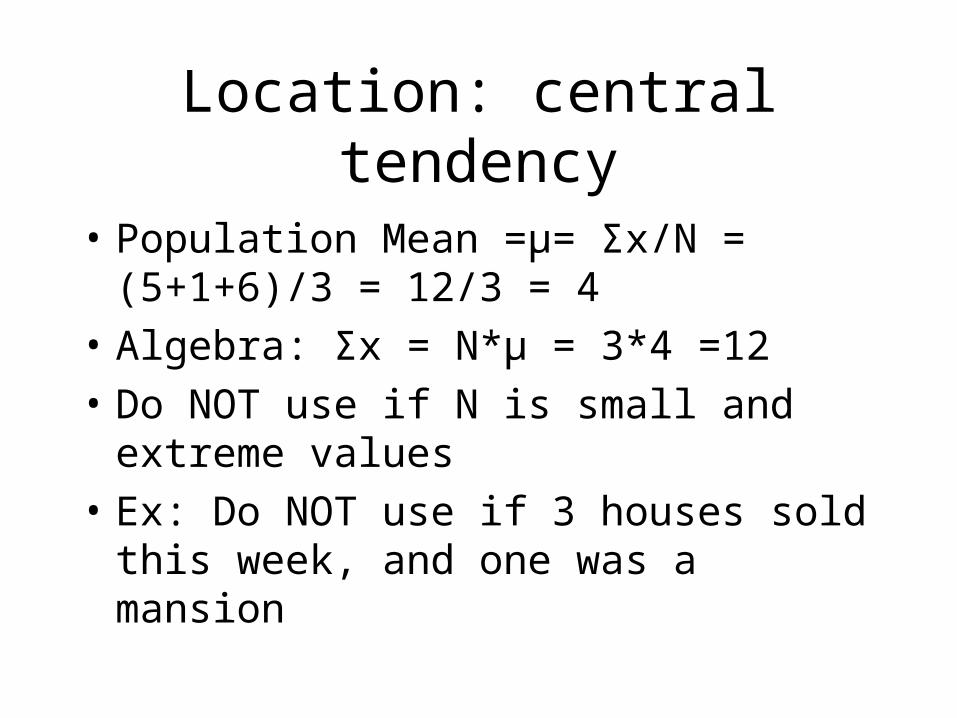
Location: central tendency
• Population Mean =µ= Σx/N = (5+1+6)/3 = 12/3 = 4
• Algebra: Σx = N*µ = 3*4 =12
• Do NOT use if N is small and extreme values
• Ex: Do NOT use if 3 houses sold this week, and one was a mansion
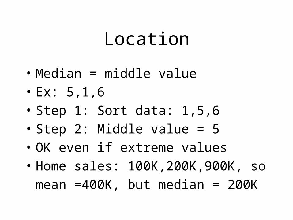
Location
• Median = middle value
• Ex: 5,1,6
• Step 1: Sort data: 1,5,6
• Step 2: Middle value = 5
• OK even if extreme values
• Home sales: 100K,200K,900K, so
mean =400K, but median = 200K
Location
• Mode: most frequent value
• Ex: female, male, female
• Mode = female
• Ex: 1,1,2,3,5,8: mode = 1

Relationship
• Case 1: if symmetric (ex bell, normal), then mean = median = mode
• Case 2: if positively skewed to right, then mode<median<mean
• Case 3: if negatively skewed to left, then mean<median<mode
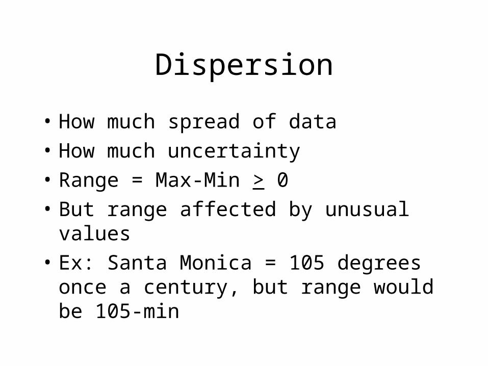
Dispersion
• How much spread of data
• How much uncertainty
• Range = Max-Min > 0
• But range affected by unusual values
• Ex: Santa Monica = 105 degrees once a century, but range would be 105-min

Standard Deviation
• Better than range because all data used
• Population SD = Square root of variance =sigma =σ
• SD > 0

Empirical Rule
• Applies to mound or bell-shaped curves
• Ex: normal distribution
• 68% of data within + one SD of mean
• 95% of data within + two SD of mean
• 99.7% of data within + three SD of mean

Sample Variance

2
1)(
nxx

Standard deviation = Square root of variance

1)( 2
nxx
s
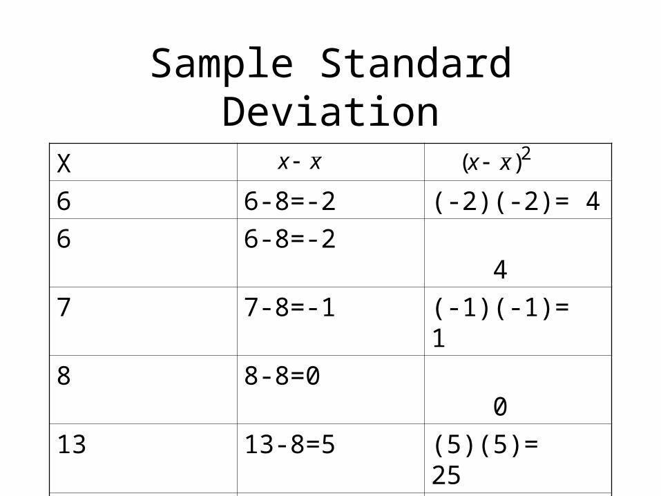
Sample Standard Deviation
X
6 6-8=-2 (-2)(-2)= 4
6 6-8=-2 4
7 7-8=-1 (-1)(-1)= 1
8 8-8=0 0
13 13-8=5 (5)(5)= 25
Sum=40 Sum=0 Sum = 34
Mean=40/5=8
xx 2)( xx
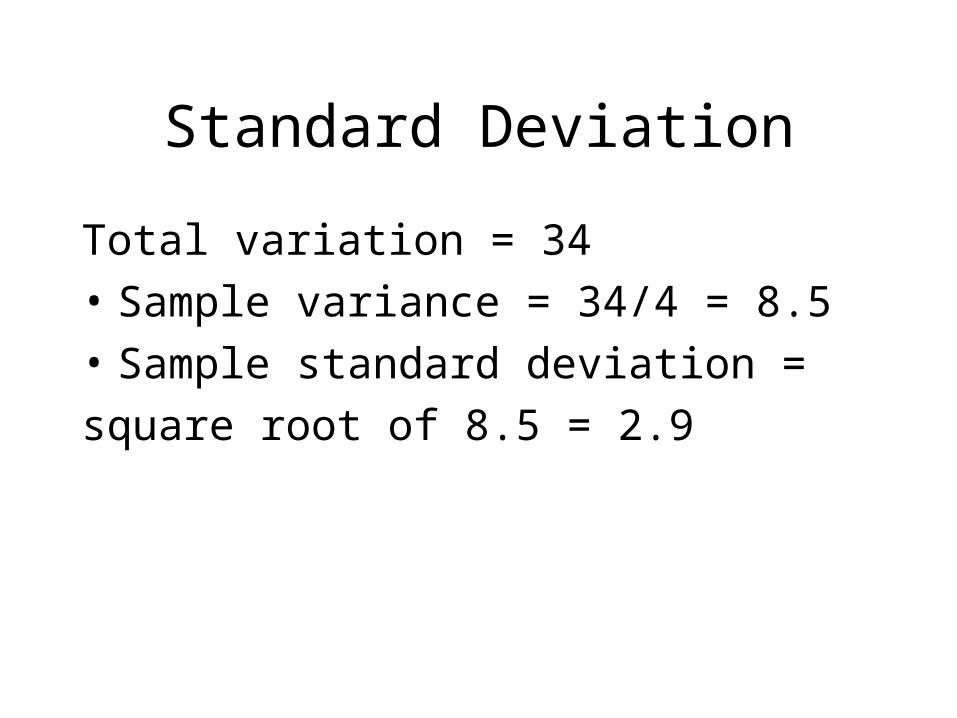
Standard Deviation
Total variation = 34
• Sample variance = 34/4 = 8.5
• Sample standard deviation =
square root of 8.5 = 2.9
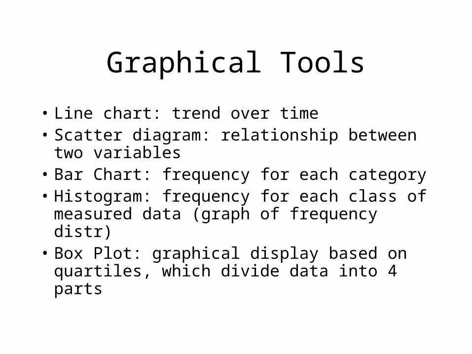
Graphical Tools
• Line chart: trend over time• Scatter diagram: relationship between two
variables• Bar Chart: frequency for each category• Histogram: frequency for each class of
measured data (graph of frequency distr)• Box Plot: graphical display based on
quartiles, which divide data into 4 parts

Top Ten #2
• Hypothesis Testing

Ho: Null Hypothesis
• Population mean=µ
• Population proportion=π
• Never include sample statistic in hypothesis

HA: Alternative Hypothesis
• ONE TAIL ALTERNATIVE– Right tail: µ>number(smog ck)
π>fraction(%defectives)
Left tail: µ<number(weight in box of crackers)
π<fraction(unpopular President’s % approval low)
Two-tail Alternative
• Population mean not equal to number (too hot or too cold)
• Population proportion not equal to fraction(% alcohol too weak or too strong)
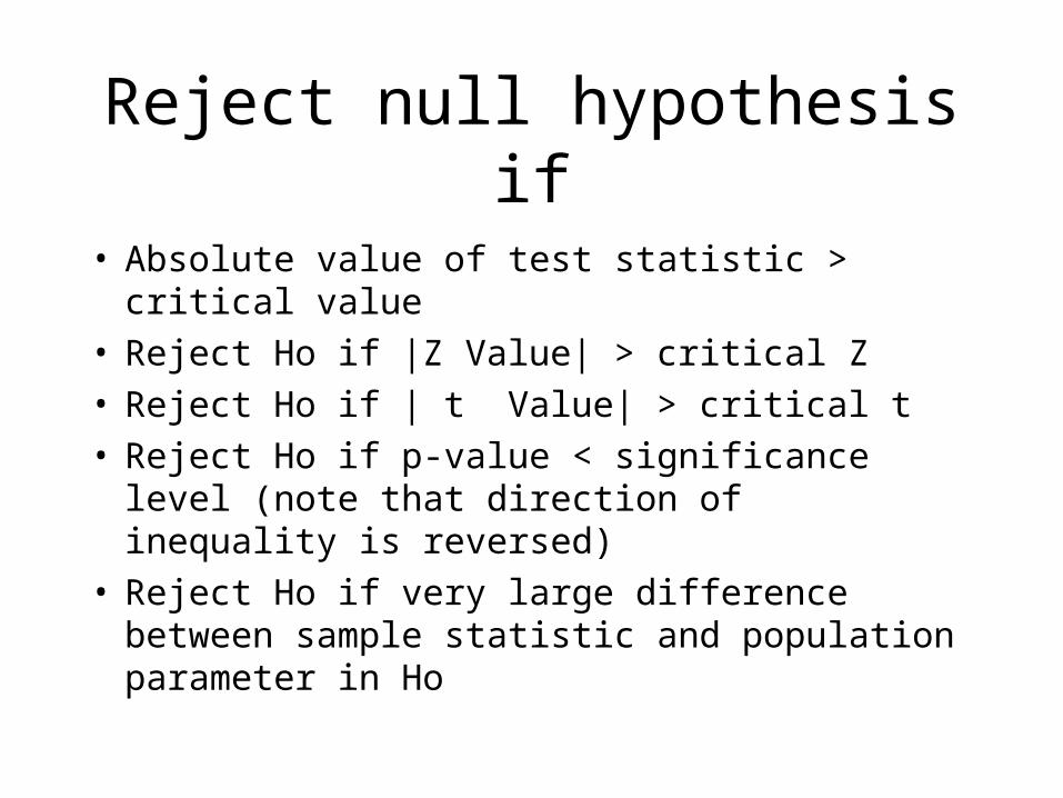
Reject null hypothesis if
• Absolute value of test statistic > critical value• Reject Ho if |Z Value| > critical Z• Reject Ho if | t Value| > critical t• Reject Ho if p-value < significance level (note that
direction of inequality is reversed)• Reject Ho if very large difference between sample
statistic and population parameter in Ho

Example: Smog Check
• Ho: µ = 80• HA: µ > 80• If test statistic =2.2 and critical value =
1.96, reject Ho, and conclude that the population mean is likely > 80
• If test statistic = 1.6 and critical value = 1.96, do not reject Ho, and reserve judgment about Ho

Type I vs Type II error
• Alpha=α = P(type I error) = Significance level = probability you reject true null hypothesis
• Ex: Ho: Defendant innocent• α = P(jury convicts innocent person)• Beta= β = P(type II error) = probability you do not
reject a null hypothesis, given Ho false
• β =P(jury acquits guilty person)

Type I vs Type II Error
Ho true Ho false
Reject Ho Alpha =α =
P(type I error)
1 – β
Do not reject Ho 1-α Beta =β =
P(type II error)
Top Ten #3
• Confidence Intervals:
Mean and Proportion
Confidence Interval: Mean
• Use normal distribution (Z table if):
population standard deviation (sigma) known and either (1) or (2):
(1) Normal population
(2) Sample size > 30

Confidence Interval: Mean
• If normal table, then µ =(Σx/n)+ Z(σ/n1/2), where n1/2 is the square root of n

Normal table
• Tail = .5(1 – confidence level)
• NOTE! Different statistics texts have different normal tables
• This review uses the tail of the bell curve
• Ex: 95% confidence: tail = .5(1-.95)= .025
• Z.025 = 1.96
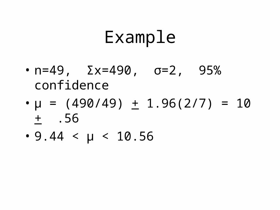
Example
• n=49, Σx=490, σ=2, 95% confidence
• µ = (490/49) + 1.96(2/7) = 10 + .56
• 9.44 < µ < 10.56

Conf. Interval: Mean t distribution
• Use if normal population but population standard deviation (σ) not known
• If you are given the sample standard deviation (s), use t table, assuming normal population
• If one population, n-1 degrees of freedom
t distribution
• µ = (Σx/n) + tn-1(s/n1/2)

Conf. Interval: Proportion
• Use if success or failure
(ex: defective or ok)
Normal approximation to binomial ok if
(n)(π) > 5 and (n)(1-π) > 5, where
n = sample size
π= population proportion
NOTE! NEVER use the t table if proportion!!

Confidence Interval: proportion
• Π= p + Z(p(1-p)/n)1/2
• Ex: 8 defectives out of 100, so p = .08 and
n = 100, 95% confidence
Π= .08 + 1.96(.08*.92/100)1/2
= .08 + .05

Interpretation
• If 95% confidence, then 95% of all confidence intervals will include the true population parameter
• NOTE! Never use the term “probability” when estimating a parameter!! (ex: Do NOT say ”Probability that population mean is between 23 and 32 is .95” because parameter is not a random variable)

Point vs Interval Estimate
• Point estimate: statistic (single number)
• Ex: sample mean, sample proportion
• Each sample gives different point estimate
• Interval estimate: range of values
• Ex: Population mean = sample mean + error
• Parameter = statistic + error
Width of Interval
• Ex: sample mean =23, error = 3
• Point estimate = 23
• Interval estimate = 23 + 3, or (20,26)
• Width of interval = 26-20 = 6
• Wide interval: Point estimate unreliable

Wide interval if
• (1) small sample size(n)• (2) large standard deviation(σ)• (3) high confidence interval (ex: 99% confidence
interval wider than 95% confidence interval)
If you want narrow interval, you need a large sample size or small standard deviation or low confidence level.

Top Ten #4: Linear Regression
• Regression equation: y=bo+b1x
• y=dependent variable=predicted value
• x= independent variable
• bo=y-intercept =predicted value of y if x=0
• b1=slope=regression coefficient
=change in y per unit change in x
Slope vs correlation
• Positive slope (b1>0): positive correlation between x and y (y incr if x incr)
• Negative slope (b1<0): negative correlation (y decr if x incr)
• Zero slope (b1=0): no correlation(predicted value for y is mean of y), no linear relationship between x and y
Simple linear regression
• Simple: one independent variable, one dependent variable
• Linear: graph of regression equation is straight line

Coefficient of determination
• R2 = % of total variation in y that can be explained by variation in x
• Measure of how close the linear regression line fits the points in a scatter diagram
• R2 = 1: max possible value: perfect linear relationship between y and x (straight line)
• R2 = 0: min value: no linear relationship

example
• Y = salary (female manager, in thousands of dollars)
• X = number of children
• n = number of observations

Given data
x y
2 48
1 52
4 33

Totals
x y
2 48
1 52
4 33 n=3
Sum=7 Sum=133
3.237 x

3.443
133 y

Slope = -6.500
• Method of Least Squares formulas not on 301 exam
• B1 = -6.500 given
Interpret slope
If one female manager has 1 more child than another, salary is $6500
lower
Intercept
bo= y – b1x
Intercept
bo=44.33-(-6.5)(2.33) = 59.5
Interpret intercept
If number of children is zero, expected salary is $59,500

Regression Equation
• Y = 59.5 – 6.5X
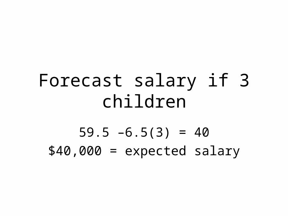
Forecast salary if 3 children
59.5 –6.5(3) = 40
$40,000 = expected salary
averagey
actualy
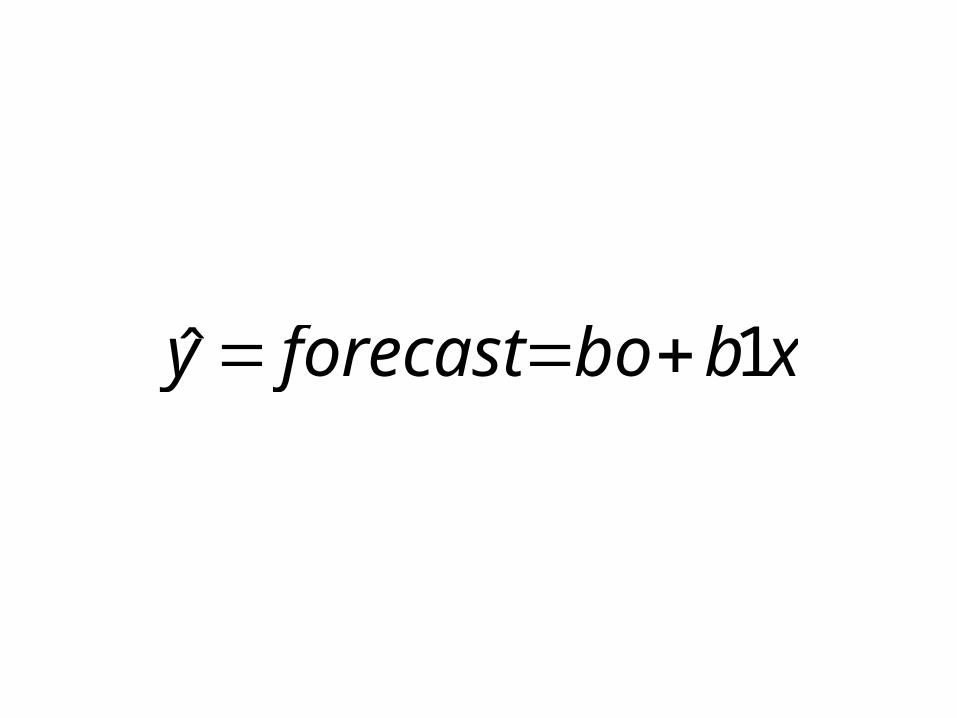
xbboforecasty 1ˆ
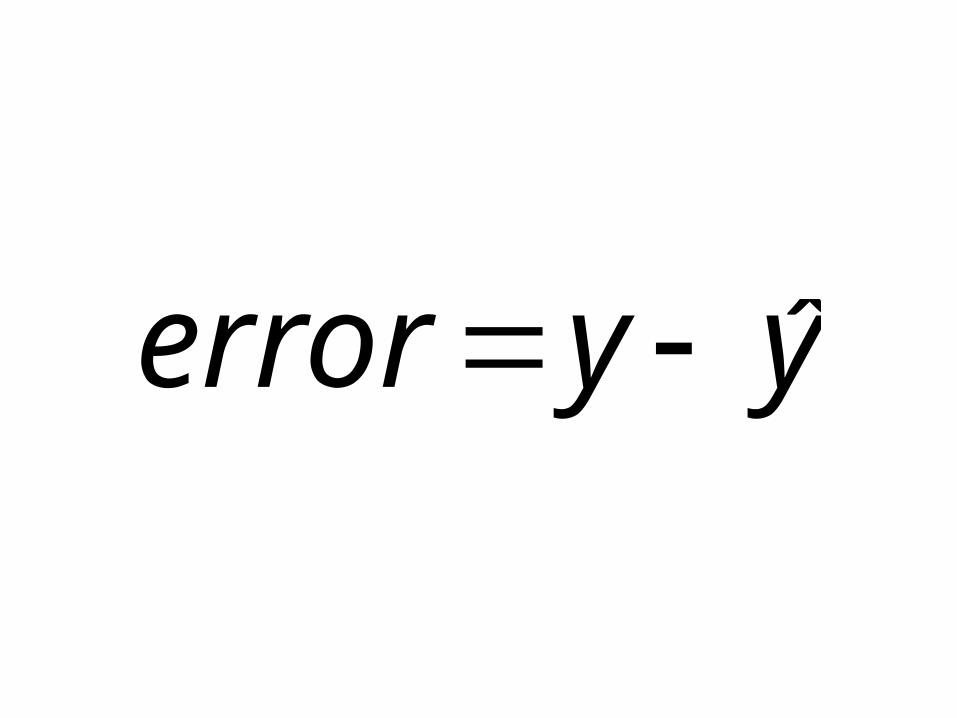
yyerror ˆ

2)ˆ( 2
nyy
S
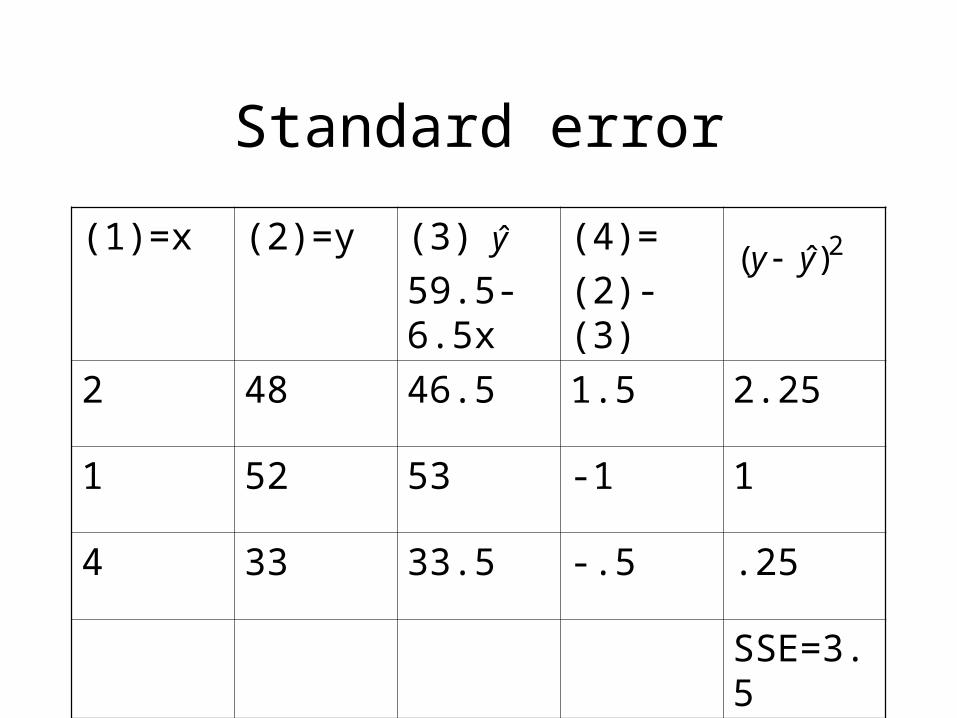
Standard error
(1)=x (2)=y (3)
59.5-6.5x
(4)=
(2)-(3)
2 48 46.5 1.5 2.25
1 52 53 -1 1
4 33 33.5 -.5 .25
SSE=3.5
y 2)ˆ( yy
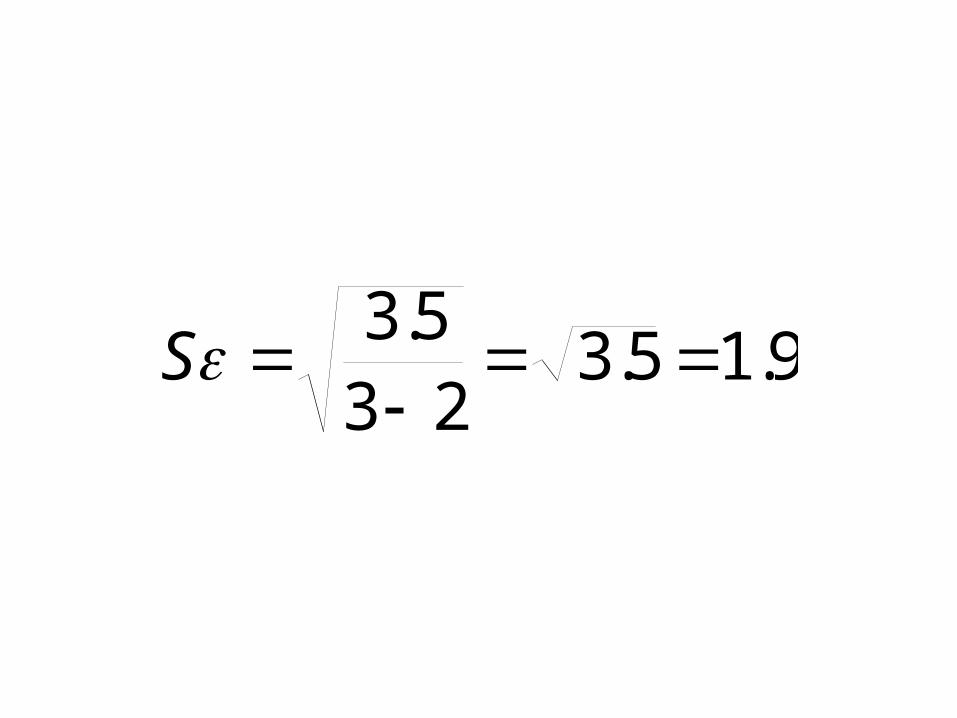
9.15.323
5.3
S

Interpret
Actual salary typically $1900 away from expected salary

• Sources of Variation (V)
• Total V = Explained V + Unexplained V
• SS = Sum of Squares = V
• Total SS = Regression SS + Error SS
• SST = SSR + SSE
• SSR = Explained V, SSE = Unexplained

Coefficient of Determination
• R2 = SSR SST
• R2 = 197 = .98 200.5
• Interpret: 98% of total variation in salary can be explained by variation in number of children

0 < R2 < 1
• 0: No linear relationship since SSR=0 (explained variation =0)
• 1: Perfect relationship since SSR = SST (unexplained variation = SSE = 0), but does not prove cause and effect

R=Correlation Coefficient
• Case 1: slope < 0
• R < 0
• R is negative square root of coefficient of determination

2RR

Our Example
• Slope = b1 = -6.5
• R2 = .98
• R = -.99
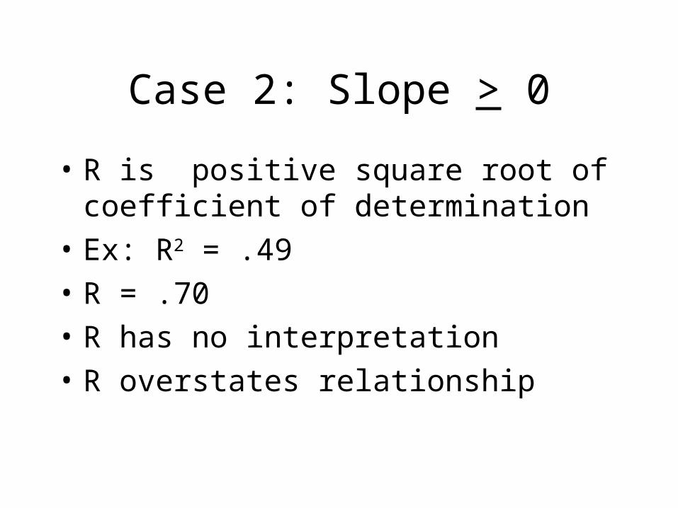
Case 2: Slope > 0
• R is positive square root of coefficient of determination
• Ex: R2 = .49
• R = .70
• R has no interpretation
• R overstates relationship
Caution
• Nonlinear relationship (parabola, hyperbola, etc) can NOT be measured by R2
• In fact, you could get R2=0 with a nonlinear graph on a scatter diagram
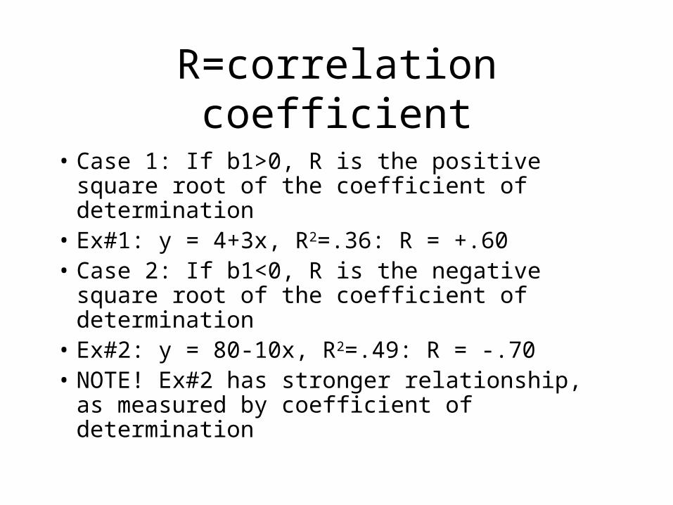
R=correlation coefficient
• Case 1: If b1>0, R is the positive square root of the coefficient of determination
• Ex#1: y = 4+3x, R2=.36: R = +.60• Case 2: If b1<0, R is the negative square
root of the coefficient of determination• Ex#2: y = 80-10x, R2=.49: R = -.70• NOTE! Ex#2 has stronger relationship, as
measured by coefficient of determination

Extreme Values
• R=+1: perfect positive correlation
• R= -1: perfect negative correlation
• R=0: zero correlation
Top Ten #5
• Expected Value = E(x) = ΣxP(x)
= x1P(x1) + x2P(x2) +…
Expected value is a weighted average, also a long-run average
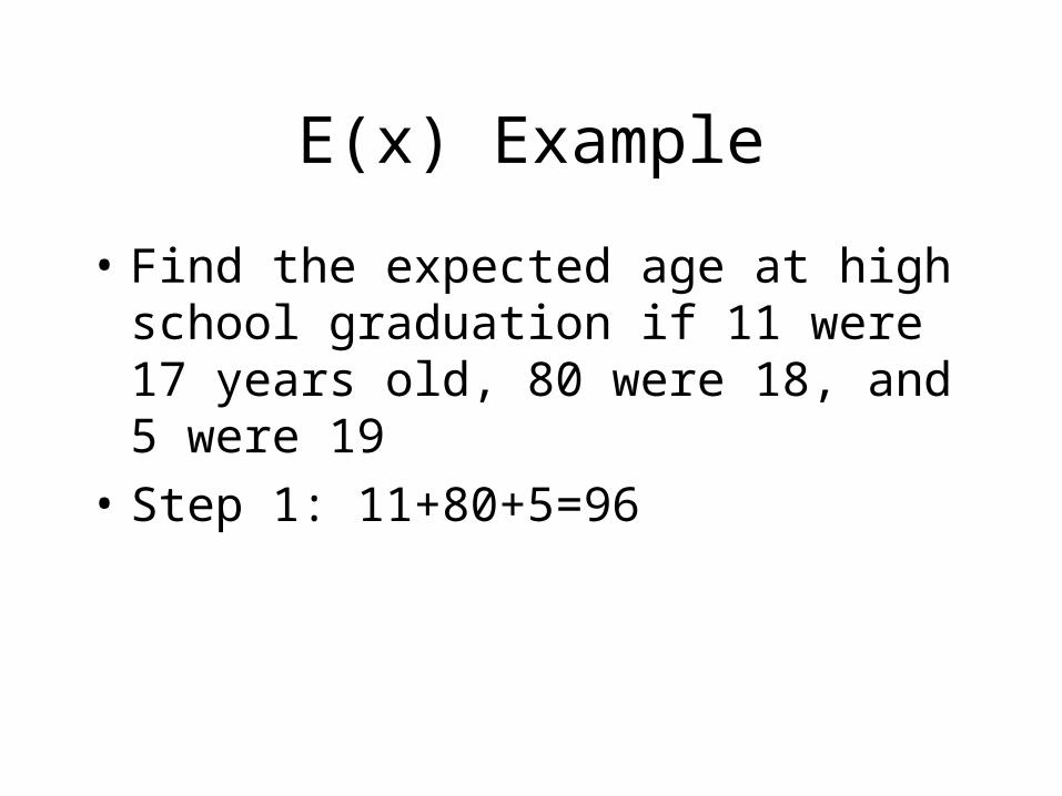
E(x) Example
• Find the expected age at high school graduation if 11 were 17 years old, 80 were 18, and 5 were 19
• Step 1: 11+80+5=96
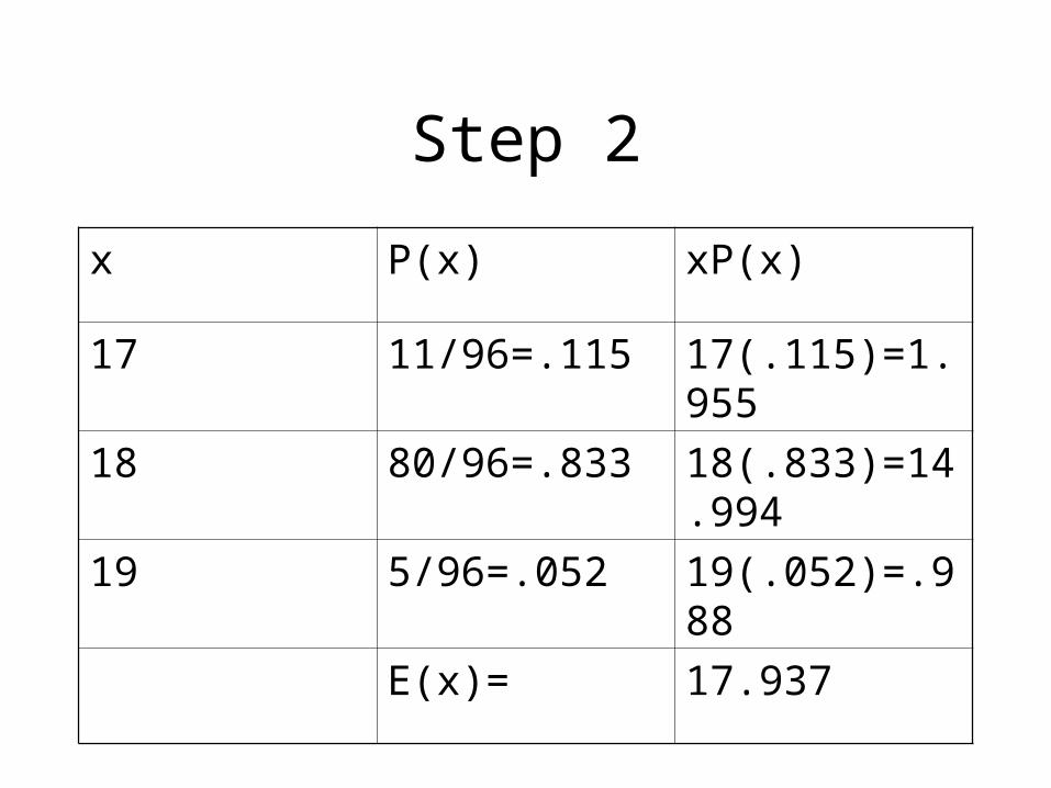
Step 2
x P(x) xP(x)
17 11/96=.115 17(.115)=1.955
18 80/96=.833 18(.833)=14.994
19 5/96=.052 19(.052)=.988
E(x)= 17.937
Top Ten #6
• What distribution to use?
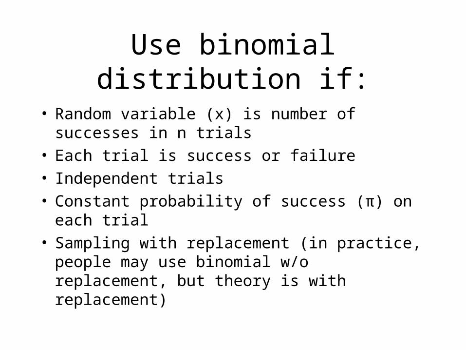
Use binomial distribution if:
• Random variable (x) is number of successes in n trials
• Each trial is success or failure• Independent trials• Constant probability of success (π) on each trial• Sampling with replacement (in practice, people
may use binomial w/o replacement, but theory is with replacement)
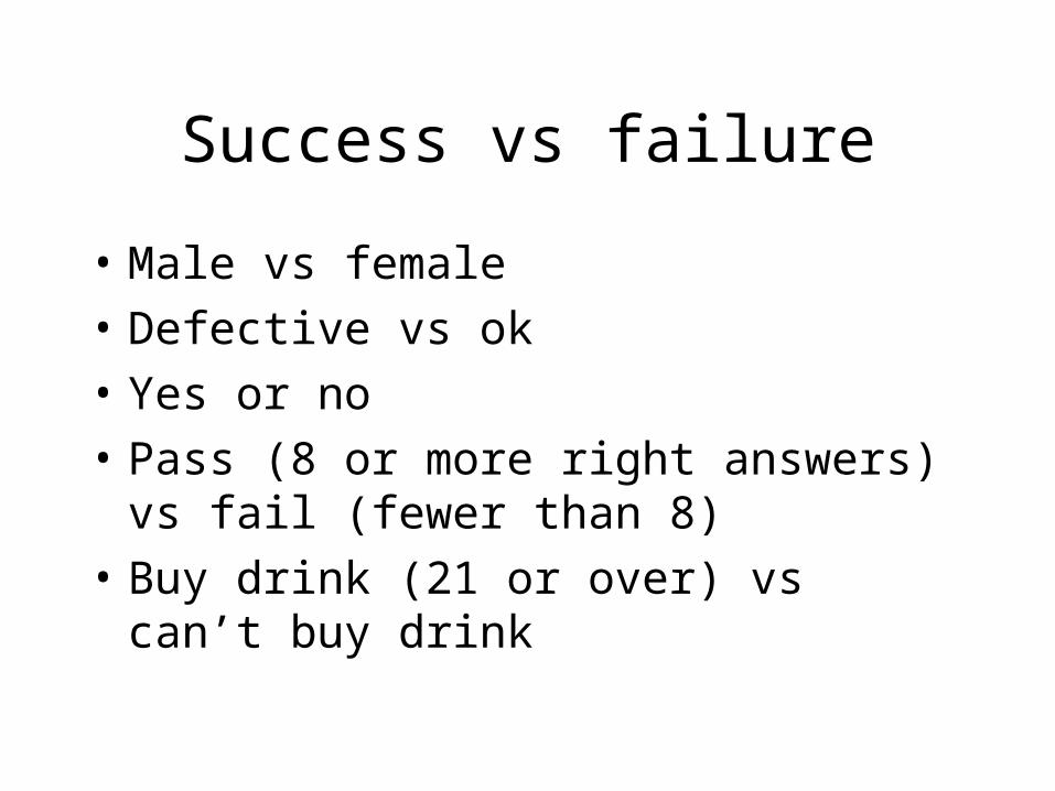
Success vs failure
• Male vs female
• Defective vs ok
• Yes or no
• Pass (8 or more right answers) vs fail (fewer than 8)
• Buy drink (21 or over) vs can’t buy drink

Binomial is discrete
• Integer values
• 0,1,2,…n
• Binomial is often skewed, but may be symmetric

Normal Distribution
• Continuous, bell-shaped, symmetric• Mean=median=mode• Measurement (dollars, inches, years)• Cumulative probability under normal curve : use Z
table if you know population mean and population standard deviation
• Sample mean: use Z table if you know population standard deviation and either normal population or n > 30

t distribution
• Continuous, bell-shaped, symmetric• Applications similar to normal• More spread out than normal• Use t if normal population but population
standard deviation not known• Degrees of freedom = df = n-1 if estimating
the mean of one population • t approaches z as df increases
Top Ten #7
• P-value = probability of getting a sample statistic as extreme (or more extreme) than the sample statistic you got from your sample
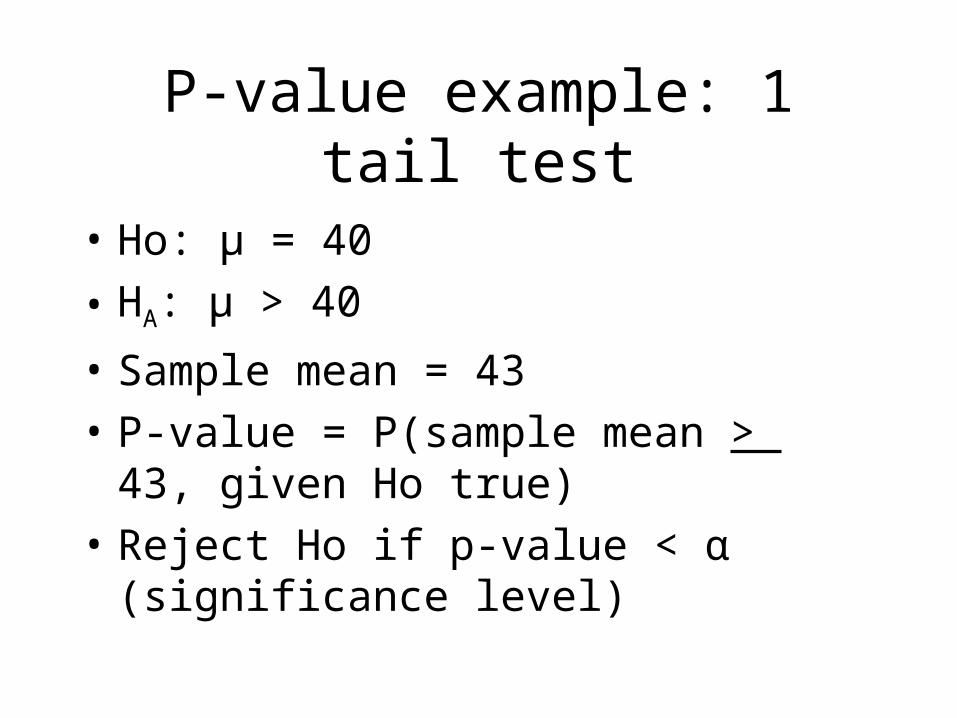
P-value example: 1 tail test
• Ho: µ = 40
• HA: µ > 40
• Sample mean = 43
• P-value = P(sample mean > 43, given Ho true)
• Reject Ho if p-value < α (significance level)
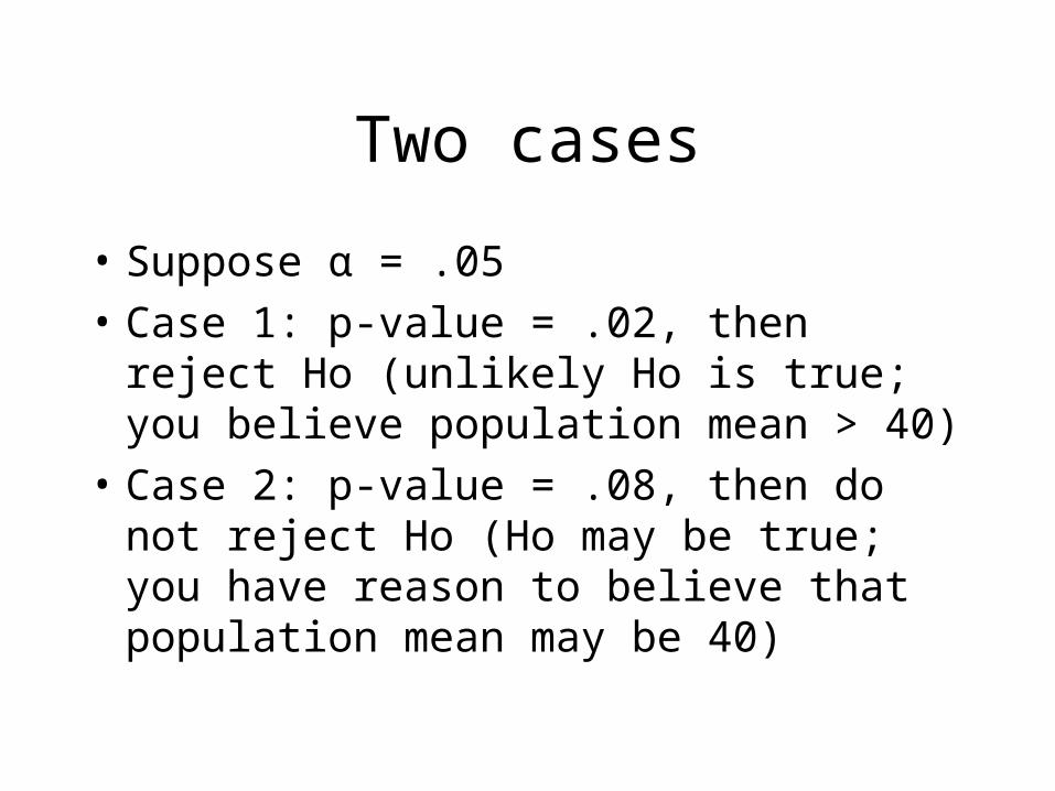
Two cases
• Suppose α = .05
• Case 1: p-value = .02, then reject Ho (unlikely Ho is true; you believe population mean > 40)
• Case 2: p-value = .08, then do not reject Ho (Ho may be true; you have reason to believe that population mean may be 40)

P-value example: 2 tail test
• Ho: µ = 70
• HA: µ not equal to 70
• Sample mean = 72
• If 2-tails, then P-value =
2*P(sample mean > 72)=2(.04)=.08
If α = .05, p-value > α, so do not reject Ho

Top Ten #8
• Variation creates uncertainty
No variation
• Certainty, exact prediction
• Standard deviation = 0
• Variance = 0
• All data exactly same
• Example: all workers in minimum wage job

High variation
• Uncertainty, unpredictable
• High standard deviation
• Ex#1: Workers in downtown L.A. have variation between CEOs and garment workers
• Ex#2: New York temperatures in spring range from below freezing to very hot
Comparing standard deviations
• Temperature Example
• Beach city: small standard deviation (single temperature reading close to mean)
• High Desert city: High standard deviation (hot days, cool nights in spring)
Standard error of the mean
• Standard deviation of sample mean =
standard deviation/square root of n
Ex: standard deviation = 10, n =4, so standard error of the mean = 10/2= 5
Note that 5<10, so standard error < standard deviation
As n increases, standard error decreases

Sampling Distribution
• Expected value of sample mean = population mean, but an individual sample mean could be smaller or larger than the population mean
• Population mean is a constant parameter, but sample mean is a random variable
• Sampling distribution is distribution of sample means

Example
• Mean age of all students in the building is population mean
• Each classroom has a sample mean
• Distribution of sample means from all classrooms is sampling distribution
Central Limit Theorem
• If population standard deviation is known, sampling distribution of sample means is normal if n > 30
• CLT applies even if original population is skewed

Top Ten #9
• Population vs sample
Population
• Collection of all items(all light bulbs made at factory)
• Parameter: measure of population
(1)population mean(average number of hours in life of all bulbs)
(2)population proportion(% of all bulbs that are defective)

Sample
• Part of population(bulbs tested by inspector)
• Statistic: measure of sample = estimate of parameter
(1) sample mean(average number of hours in life of bulbs tested by inspector)
(2) sample proportion(% of bulbs in sample that are defective)

Top Ten #10
• Qualitative vs quantitative

Qualitative
• Categorical data
success vs failure
ethnicity
marital status
color
zip code
4 star hotel in tour guide

Qualitative
• If you need an “average”, do not calculate the mean
• However, you can compute the mode (“average” person is married, buys a blue car made in America)

Quantitative
• 2 cases
• Case 1: discrete
• Case 2: continuous
Discrete
(1) integer values (0,1,2,…)
(2) example: binomial
(3) finite number of possible values
(4) counting
(5) number of brothers
(6) number of cars arriving at gas station

Continuous
• Real numbers, such as decimal values ($22.22)
• Examples: Z, t
• Infinite number of possible values
• Measurement
• Miles per gallon, distance, duration of time
Graphical tools
• Pie chart or bar chart: qualitative
• Joint frequency table: qualitative (relate marital status vs zip code)
• Scatter diagram: quantitative (distance from CSUN vs duration of time to reach CSUN)

Hypothesis testingConfidence intervals
• Quantitative: Mean
• Qualitative: Proportion