topic models and latent dirichlet allocation · topic models and latent dirichlet allocation kevin...
TRANSCRIPT
Topic Models and Latent Dirichlet Allocation
Kevin Yang and Zachary Wu
27 April 2017
CS 159 1
Motivation
We want to find short descriptions of the members of a collection
that
Ienable e�cient processing of large collections
Ipreserve essential statistical relationships
Ithat can be used for classification, novelty detection,
summarization, and similarity and relevance judgments
CS 159 2
Words, documents, and corpora
IWords are discrete units of data and belong to a vocabulary of
size V .
IWords are encoded by one-hot vectors of length V .
IA document is a sequence of N words denoted
w = (w1,w2, ...wN
)
IA corpus is a collection of M documents denoted
D = {w1,w2, ...,wM
}
CS 159 3
Latent Dirichlet Allocation
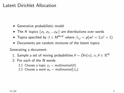
IGenerative probabilistic model
IThe K topics {z1, z2, ...z
K
} are distributions over words
ITopics specified by � 2 M
KxV
where �i ,j = p(w
j
= 1|z j = 1)
IDocuments are random mixtures of the latent topics
Generating a document:
1. Sample a set of mixing probabilities ✓ ⇠ Dir(↵), ↵, ✓ 2 RK
2. For each of the N words:
2.1 Choose a topic z
n
⇠ multinomial(✓)2.2 Choose a word w
n
⇠ multinomial(�n
)
CS 159 4
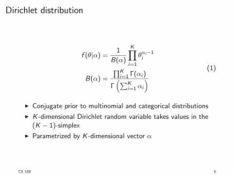
Dirichlet distribution
f (✓|↵) = 1
B(↵)
KY
i=1
✓↵i
�1i
B(↵) =
QK
i=1 �(↵i
)
�
⇣PK
i=1 ↵i
⌘(1)
IConjugate prior to multinomial and categorical distributions
IK -dimensional Dirichlet random variable takes values in the
(K � 1)-simplex
IParametrized by K -dimensional vector ↵
CS 159 5
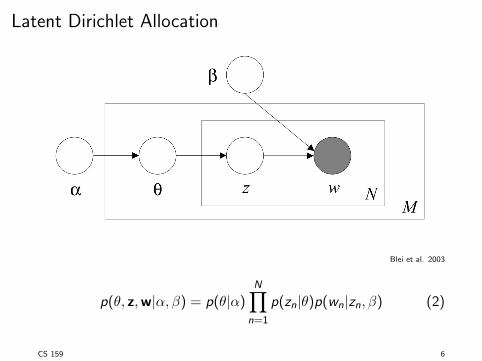
Latent Dirichlet Allocation
Blei et al. 2003
p(✓, z,w|↵,�) = p(✓|↵)NY
n=1
p(z
n
|✓)p(wn
|zn
,�) (2)
CS 159 6
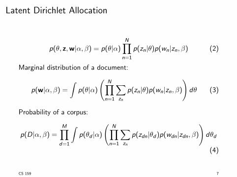
Latent Dirichlet Allocation
p(✓, z,w|↵,�) = p(✓|↵)NY
n=1
p(z
n
|✓)p(wn
|zn
,�) (2)
Marginal distribution of a document:
p(w|↵,�) =Z
p(✓|↵)
NY
n=1
X
z
n
p(z
n
|✓)p(wn
|zn
,�)
!d✓ (3)
Probability of a corpus:
p(D|↵,�) =MY
d=1
Zp(✓
d
|↵)
NY
n=1
X
z
n
p(z
dn
|✓d
)p(w
dn
|zdn
,�)
!d✓
d
(4)
CS 159 7

Exchangeability
A finite set of random variable {z1, ..., zN
} is exchangeable if the
joint distribution is invariant to permutation. That is, for a
permutation ⇡ of the integers from 1 to N:
p(z1, ..., zN
) = p(z⇡(1), ..., z⇡(N))
An infinite sequence of random variables is infinitely exchangeable
if every finite subsequence is exchangeable.
CS 159 8
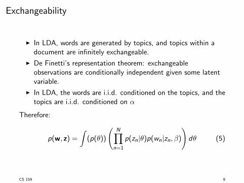
Exchangeability
IIn LDA, words are generated by topics, and topics within a
document are infinitely exchangeable.
IDe Finetti’s representation theorem: exchangeable
observations are conditionally independent given some latent
variable.
IIn LDA, the words are i.i.d. conditioned on the topics, and the
topics are i.i.d. conditioned on ↵
Therefore:
p(w, z) =
Z(p(✓))
NY
n=1
p(z
n
|✓)p(wn
|zn
,�)
!d✓ (5)
CS 159 9
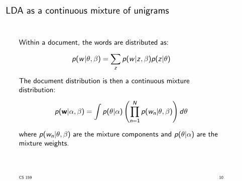
LDA as a continuous mixture of unigrams
Within a document, the words are distributed as:
p(w |✓,�) =X
z
p(w |z ,�)p(z |✓)
The document distribution is then a continuous mixture
distribution:
p(w|↵,�) =Z
p(✓|↵)
NY
n=1
p(w
n
|✓,�)!d✓
where p(w
n
|✓,�) are the mixture components and p(✓|↵) are the
mixture weights.
CS 159 10
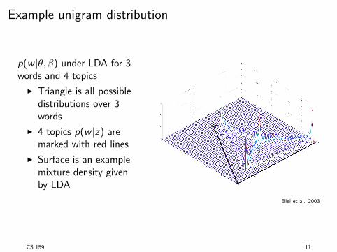
Example unigram distribution
p(w |✓,�) under LDA for 3
words and 4 topics
ITriangle is all possible
distributions over 3
words
I4 topics p(w |z) aremarked with red lines
ISurface is an example
mixture density given
by LDA
Blei et al. 2003
CS 159 11
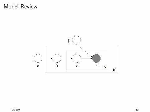
Model Review
CS 159 12
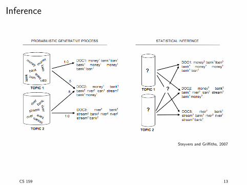
Inference
Steyvers and Gri�ths, 2007
CS 159 13
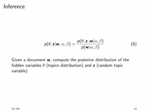
Inference
p(✓, z|w,↵,�) =p(✓, z,w|↵,�)p(w|↵,�) (6)
Given a document w, compute the posterior distribution of the
hidden variables ✓ (topics distribution) and z (random topic
variable)
CS 159 14

Inference - Numerator
The numerator of the posterior can be decomposed by the
hierarchy shown in the graphical model
p(✓, z,w|↵,�) = p(w|z,�)p(z|✓)p(✓|↵) (7)
The first term represents the probability of observing a document
w given a topic vector that assigns a topic to each word from the
probability matrix �.
p(w|z,�) =NY
n=1
�z
n
,wn
✓z
n
(8)
CS 159 15
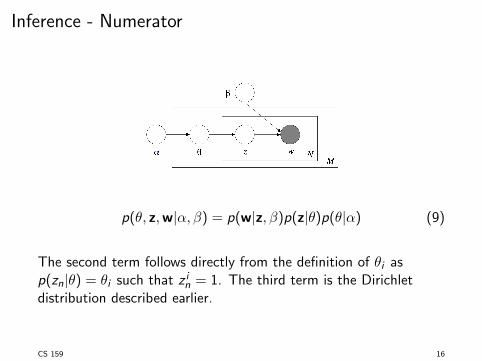
Inference - Numerator
p(✓, z,w|↵,�) = p(w|z,�)p(z|✓)p(✓|↵) (9)
The second term follows directly from the definition of ✓i
as
p(z
n
|✓) = ✓i
such that z
i
n
= 1. The third term is the Dirichlet
distribution described earlier.
CS 159 16
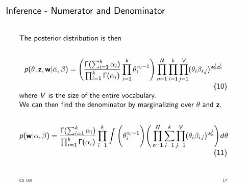
Inference - Numerator and Denominator
The posterior distribution is then
p(✓, z,w|↵,�) = �(
Pk
i=1 ↵i
)
Qk
i=1 �(↵i
)
kY
i=1
✓↵i
�1i
!NY
n=1
kY
i=1
VY
j=1
(✓i
�i ,j)
w
j
n
z
j
n
(10)
where V is the size of the entire vocabulary.
We can then find the denominator by marginalizing over ✓ and z.
p(w|↵,�) = �(
Pk
i=1 ↵i
)
Qk
i=1 �(↵i
)
kY
i=1
Z ✓↵i
�1i
! NY
n=1
kX
i=1
VY
j=1
(✓i
�i ,j)
w
j
n
!d✓
(11)
CS 159 17

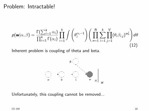
Problem: Intractable!
p(w|↵,�) = �(
Pk
i=1 ↵i
)
Qk
i=1 �(↵i
)
kY
i=1
Z ✓↵i
�1i
! NY
n=1
kX
i=1
VY
j=1
(✓i
�i ,j)
w
j
n
!d✓
(12)
Inherent problem is coupling of theta and beta.
Unfortunately, this coupling cannot be removed...
CS 159 18
Problem: Intractable!
p(w|↵,�) = �(
Pk
i=1 ↵i
)
Qk
i=1 �(↵i
)
kY
i=1
Z ✓↵i
�1i
! NY
n=1
kX
i=1
VY
j=1
(✓i
�i ,j)
w
j
n
!d✓
(12)
Inherent problem is coupling of theta and beta.
Unfortunately, this coupling cannot be removed...
CS 159 18
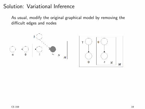
Solution: Variational Inference
As usual, modify the original graphical model by removing the
di�cult edges and nodes
Variational Distribution
q(✓, z |�,�) = q(✓|�)NY
n=1
q(z
n
|�n
) (13)
CS 159 19
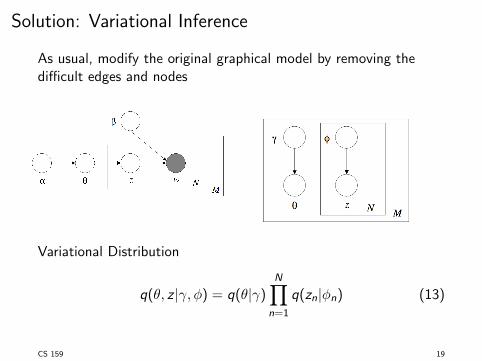
Solution: Variational Inference
As usual, modify the original graphical model by removing the
di�cult edges and nodes
Variational Distribution
q(✓, z |�,�) = q(✓|�)NY
n=1
q(z
n
|�n
) (13)
CS 159 19
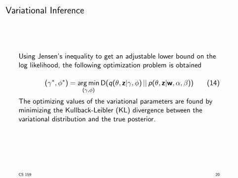
Variational Inference
Using Jensen’s inequality to get an adjustable lower bound on the
log likelihood, the following optimization problem is obtained
(�⇤,�⇤) = argmin
(�,�)D(q(✓, z|�,�) || p(✓, z|w,↵,�)) (14)
The optimizing values of the variational parameters are found by
minimizing the Kullback-Leibler (KL) divergence between the
variational distribution and the true posterior.
CS 159 20
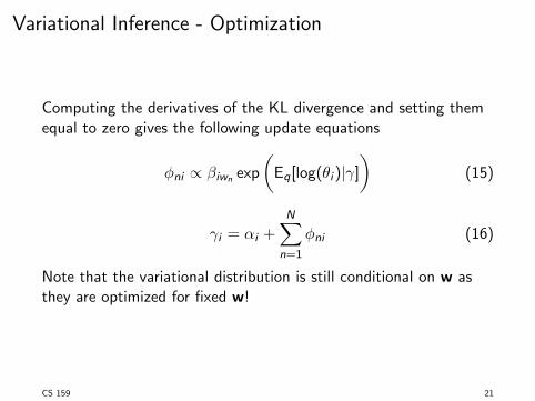
Variational Inference - Optimization
Computing the derivatives of the KL divergence and setting them
equal to zero gives the following update equations
�ni
/ �iw
n
exp
✓E
q
[log(✓i
)|�]◆
(15)
�i
= ↵i
+
NX
n=1
�ni
(16)
Note that the variational distribution is still conditional on w as
they are optimized for fixed w!
CS 159 21
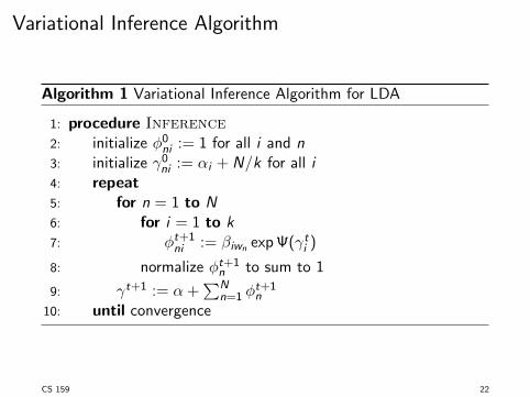
Variational Inference Algorithm
Algorithm 1 Variational Inference Algorithm for LDA
1: procedure Inference2: initialize �0
ni
:= 1 for all i and n
3: initialize �0ni
:= ↵i
+ N/k for all i
4: repeat
5: for n = 1 to N
6: for i = 1 to k
7: �t+1ni
:= �iw
n
exp (�ti
)
8: normalize �t+1n
to sum to 1
9: �t+1:= ↵+
PN
n=1 �t+1n
10: until convergence
CS 159 22
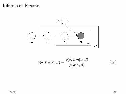
Inference: Review
p(✓, z|w,↵,�) =p(✓, z,w|↵,�)p(w|↵,�) (17)
Not done yet!
CS 159 23
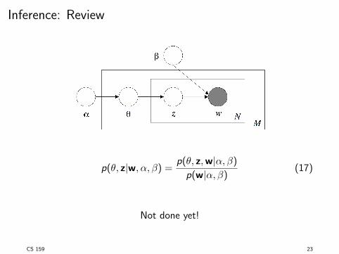
Inference: Review
p(✓, z|w,↵,�) =p(✓, z,w|↵,�)p(w|↵,�) (17)
Not done yet!
CS 159 23
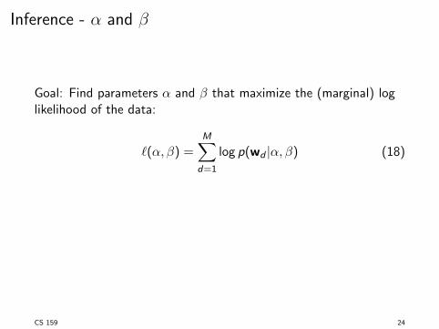
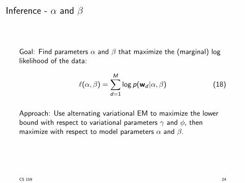
Inference - ↵ and �
Goal: Find parameters ↵ and � that maximize the (marginal) log
likelihood of the data:
`(↵,�) =MX
d=1
log p(w
d
|↵,�) (18)
Approach: Use alternating variational EM to maximize the lower
bound with respect to variational parameters � and �, thenmaximize with respect to model parameters ↵ and �.
CS 159 24
Inference - Variational EM
1. E-Step: Find optimizing values of variational parameters
[�⇤,�⇤] as shown previously
2. Maximize the resulting lower bound on log likelihood with
respect to model parameters [↵⇤,�⇤]
CS 159 25
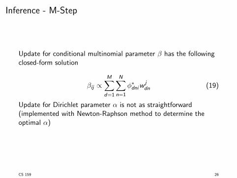
Inference - M-Step
Update for conditional multinomial parameter � has the following
closed-form solution
�ij
/MX
d=1
NX
n=1
�⇤dni
w
j
dn
(19)
Update for Dirichlet parameter ↵ is not as straightforward
(implemented with Newton-Raphson method to determine the
optimal ↵)
CS 159 26
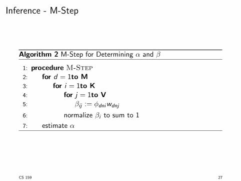
Inference - M-Step
Algorithm 2 M-Step for Determining ↵ and �
1: procedure M-Step2: for d = 1to M
3: for i = 1to K
4: for j = 1to V
5: �ij
:= �dni
w
dnj
6: normalize �i
to sum to 1
7: estimate ↵
CS 159 27
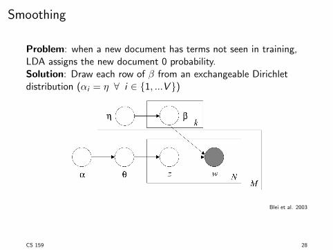
Smoothing
Problem: when a new document has terms not seen in training,
LDA assigns the new document 0 probability.
Solution: Draw each row of � from an exchangeable Dirichlet
distribution (↵i
= ⌘ 8 i 2 {1, ...V })
Blei et al. 2003
CS 159 28
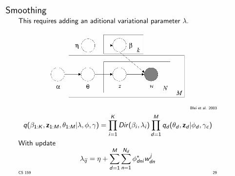
SmoothingThis requires adding an aditional variational parameter �.
Blei et al. 2003
q(�1:K , z1:M , ✓1:M |�,�, �) =KY
i=1
Dir(�i
,�i
)
MY
d=1
q
d
(✓d
, zd
|�d
, �c
)
With update
�ij
= ⌘ +MX
d=1
N
dX
n=1
�⇤dni
w
j
dn
CS 159 29

LDA results example
Topicsalgorithms organic
chemistry neuroscience solar system HIV/AIDS
Top
10 te
rms
Blei et al. 2009
CS 159 30
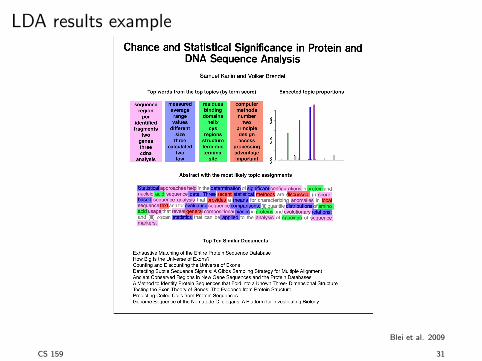
LDA results example
Blei et al. 2009
CS 159 31
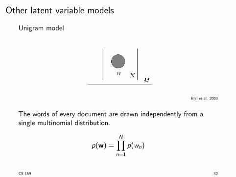
Other latent variable models
Unigram model
Blei et al. 2003
The words of every document are drawn independently from a
single multinomial distribution.
p(w) =
NY
n=1
p(w
n
)
CS 159 32
Other latent variable models
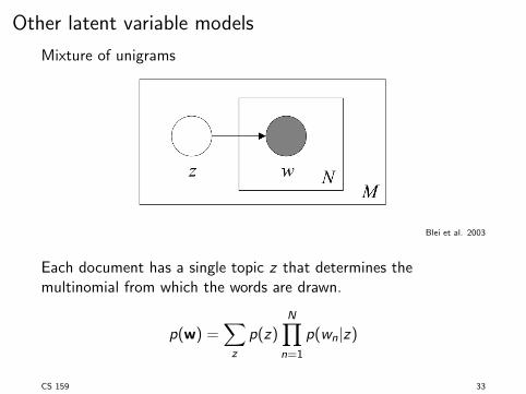
Mixture of unigrams
Blei et al. 2003
Each document has a single topic z that determines the
multinomial from which the words are drawn.
p(w) =
X
z
p(z)
NY
n=1
p(w
n
|z)
CS 159 33
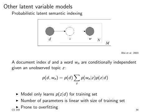
Other latent variable modelsProbabilistic latent semantic indexing
Blei et al. 2003
A document index d and a word w
n
are conditionally independent
given an unobserved topic z :
p(d ,wn
) = p(d)
X
z
p(w
n
|z)p(z |d)
IModel only learns p(z |d) for training set
INumber of parameters is linear with size of training set
IProne to overfitting
CS 159 34
Comparison of latent variable models
ITest generalization performance on unlabeled corpus.
ITrain, then measure likelihood on held-out test set.
ILower perplexity indicates better generalization
perplexity(D
test
) = exp
�P
N
d=1 log p(wd
)
PM
d=1 Nd
!
CS 159 35
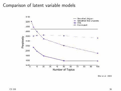
Comparison of latent variable models
Blei et al. 2003
CS 159 36
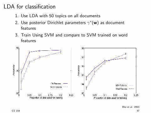
LDA for classification
1. Use LDA with 50 topics on all documents
2. Use posterior Dirichlet parameters �⇤(w) as document
features
3. Train Using SVM and compare to SVM trained on word
features
Blei et al. 2003
CS 159 37

LDA for collaborative filtering
1. Users as documents; preferred movie choices as words.
2. Train LDA on fully observed set of users.
3. For each unobserved user, hold out one movie and evaluate
probability assigned to that movie.
Blei et al. 2003CS 159 38
Extensions of LDA
ICorrelated topic model (CTM): model correlations between
occurrences of topics
IDynamic topic model (DTM): remove exchangeability
between documents to model evolution of corpus over time.
CS 159 39
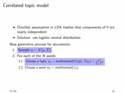
Correlated topic model
IDirichlet assumption in LDA implies that components of ✓ are
nearly independent.
ISolution: use logistic normal distribution
New generative process for documents:
1. Sample ⌘ ⇠ N (µ,⌃)
2. For each of the N words:
2.1 Choose a topic z
n
⇠ multinomial(f (⌘)), f (⌘i
) =
e
⌘iP
j
e
⌘j
2.2 Choose a word w
n
⇠ multinomial(�n
)
CS 159 40
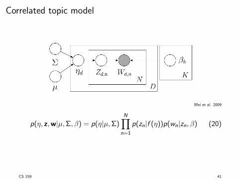
Correlated topic model
Blei et al. 2009
p(⌘, z,w|µ,⌃,�) = p(⌘|µ,⌃)NY
n=1
p(z
n
|f (⌘))p(wn
|zn
,�) (20)
CS 159 41
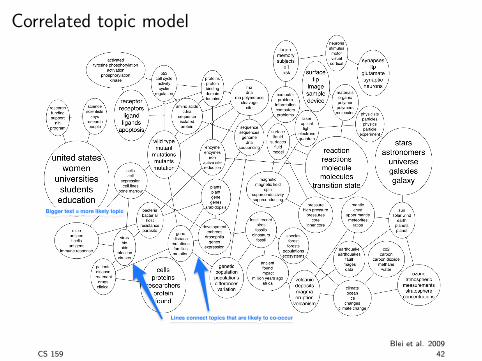
Correlated topic model
Bigger text = more likely topicBigger text = more likely topic
Lines connect topics that are likely to co-occurLines connect topics that are likely to co-occur
Blei et al. 2009CS 159 42
Dynamic topic model
IMany corpora, such as journals, email, news, and search logs
reflect evolving content.
IFor example, a neuroscience article written in 1903 would be
very di↵erent from one written in 2017.
IA DTM captures the evolution of topics in a
sequentially-organized corpus.
IDocuments are divided into time-slices (e.g. by year).
IThe topics associated with slice t evolve from those
associated with slice t � 1.
CS 159 43
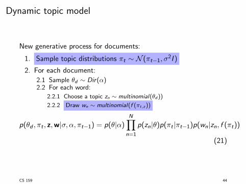
Dynamic topic model
New generative process for documents:
1. Sample topic distributions ⇡t
⇠ N (⇡t�1,�2I )
2. For each document:
2.1 Sample ✓d
⇠ Dir(↵)2.2 For each word:
2.2.1 Choose a topic z
n
⇠ multinomial(✓d
))
2.2.2 Draw w
n
⇠ multinomial(f (⇡t,z))
p(✓d
,⇡t
, z,w|�,↵,⇡t�1) = p(✓|↵)
NY
n=1
p(z
n
|✓)p(⇡t
|⇡t�1)p(wn
|zn
, f (⇡t
))
(21)
CS 159 44
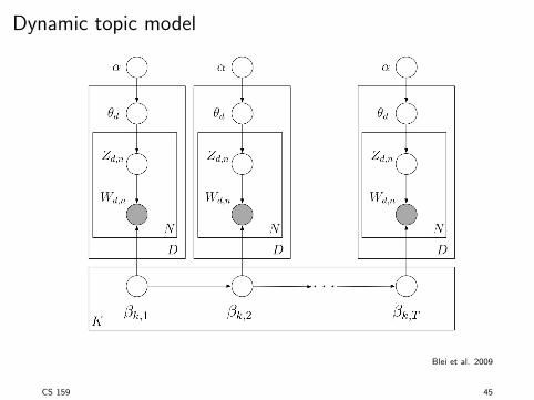
Dynamic topic model
Blei et al. 2009
CS 159 45
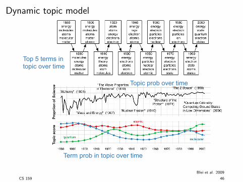
Dynamic topic model
Top 5 terms in topic over time
Topic prob over time
Term prob in topic over time
Blei et al. 2009
CS 159 46
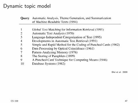
Dynamic topic model
Blei et al. 2009
CS 159 47
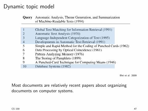
Dynamic topic model
Blei et al. 2009
Most documents are relatively recent papers about organizing
documents on computer systems.
CS 159 47
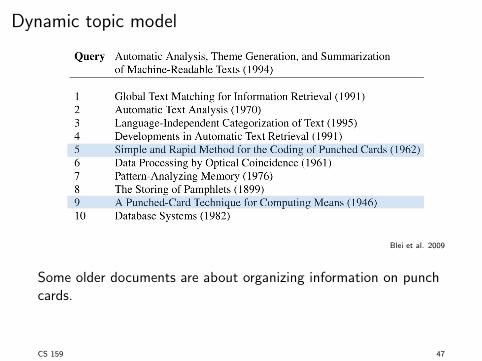
Dynamic topic model
Blei et al. 2009
Some older documents are about organizing information on punch
cards.
CS 159 47
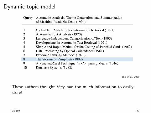
Dynamic topic model
Blei et al. 2009
These authors thought they had too much information to easily
store!
CS 159 47
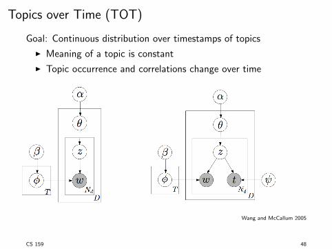
Topics over Time (TOT)
Goal: Continuous distribution over timestamps of topics
IMeaning of a topic is constant
ITopic occurrence and correlations change over time
Wang and McCallum 2005
CS 159 48
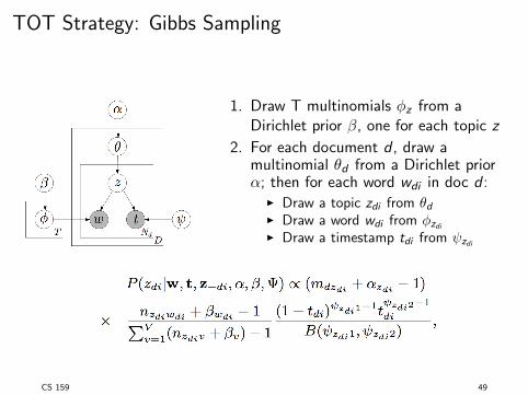
TOT Strategy: Gibbs Sampling
1. Draw T multinomials �z
from a
Dirichlet prior �, one for each topic z
2. For each document d , draw a
multinomial ✓d
from a Dirichlet prior
↵; then for each word w
di
in doc d :
IDraw a topic z
di
from ✓d
IDraw a word w
di
from �z
di
IDraw a timestamp t
di
from z
di
CS 159 49
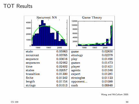
TOT Results
Wang and McCallum 2005
CS 159 50