topic13:& radiometry& - university of torontomoore/csc418/lectures/lect… · ·...
TRANSCRIPT

1
Topic 13: Radiometry
• The big picture • Measuring light coming from a light source • Measuring light falling onto a patch: Irradiance • Measuring light leaving a patch: Radiance • The Light Transport Cycle • The BidirecAonal Reflectance DistribuAon FuncAon
The Basic “Light Transport” Path
2
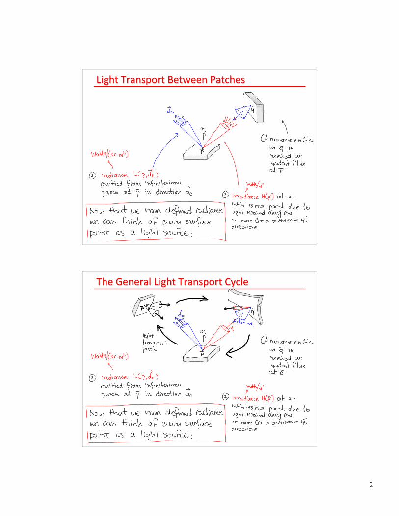
Light Transport Between Patches
The General Light Transport Cycle

3
One Step Along Path: DirecAonal IntegraAon
One Step Along Path: DirecAonal IntegraAon

4
Topic 13: Radiometry
• The big picture • Measuring light coming from a light source • Measuring light falling onto a patch: Irradiance • Measuring light leaving a patch: Radiance • The Light Transport Cycle • The BidirecAonal Reflectance DistribuAon FuncAon
General Light Transport Cycle: Closing the Loop

5
DefiniAon: The BRDF of a Point
DefiniAon: The BRDF of a Point

6
DefiniAon: The BRDF of a Point
Radiance Due to a Point Light Source

7
Radiance Due to an Extended Source
Radiance Due to an Extended Source
8
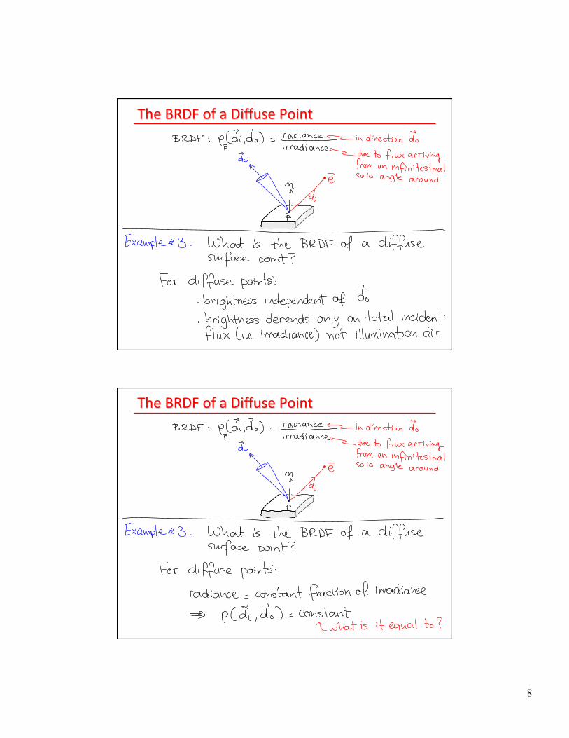
The BRDF of a Diffuse Point
The BRDF of a Diffuse Point
9
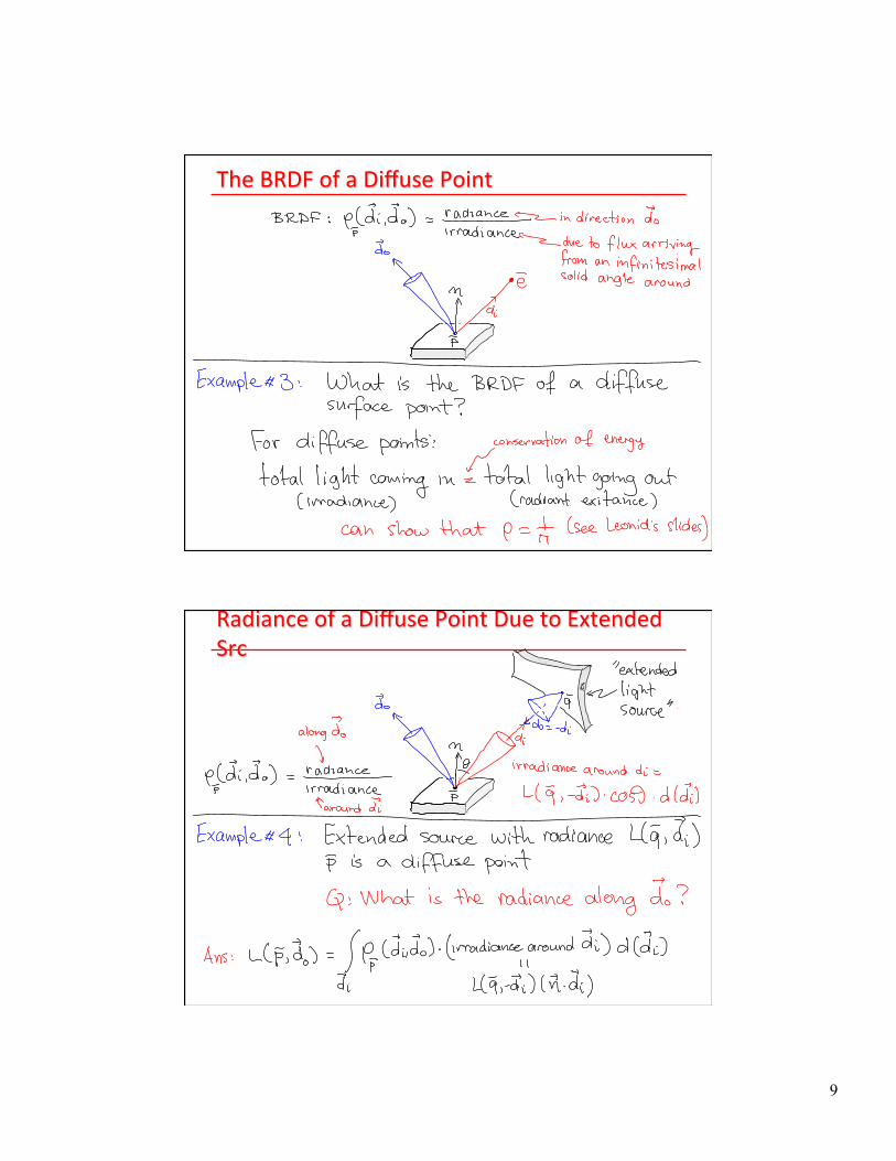
The BRDF of a Diffuse Point
Radiance of a Diffuse Point Due to Extended Src
10
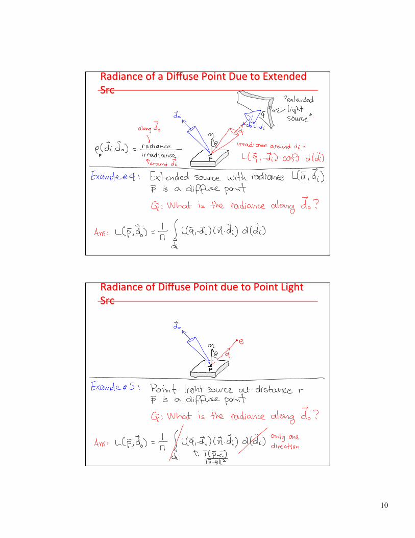
Radiance of a Diffuse Point Due to Extended Src
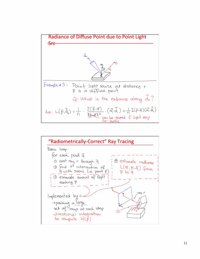
Radiance of Diffuse Point due to Point Light Src
11
Radiance of Diffuse Point due to Point Light Src
“Radiometrically-‐Correct” Ray Tracing

1
Distribution Ray Tracing
n In Whitted Ray Tracing we computed lighting very crudely q Phong + specular global lighting
n In Distributed Ray Tracing we want to compute the lighting as accurately as possible q Use the formalism of Radiometry q Compute irradiance at each pixel (by integrating all the
incoming light) q Since integrals are can not be done analytically, we will
employ numeric approximations
Benefits of Distribution Ray Tracing
n Better global diffuse lighting q Color bleeding q Bouncing highlights
n Extended light sources n Anti-aliasing n Motion blur n Depth of field n Subsurface scattering
2
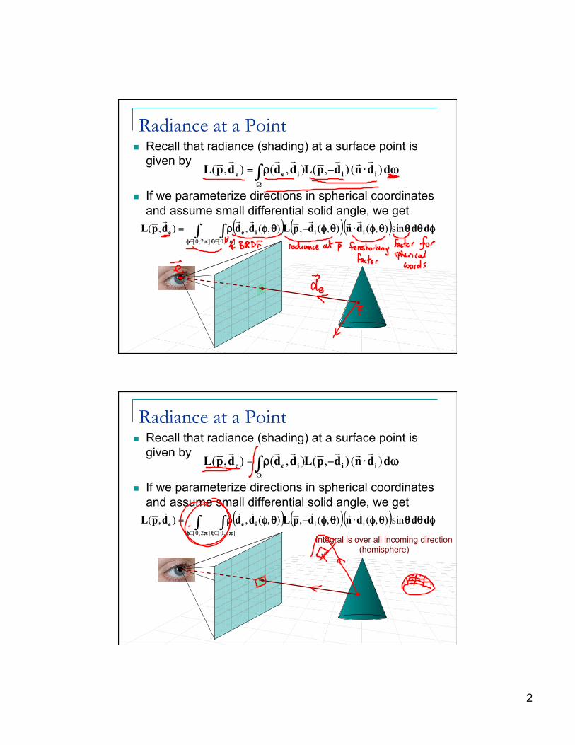
Radiance at a Point n Recall that radiance (shading) at a surface point is
given by
n If we parameterize directions in spherical coordinates and assume small differential solid angle, we get
ωρ ddndpLdddpL iiiee )(),(),(),(⋅−= ∫
Ω
( ) ( )( ) φθθθφθφθφρπφ πθ
dddndpLdddpL iiiee ∫ ∫∈ ∈
⋅−=]2,0[ ]2,0[
sin),(),(,),(,),(
Integral is over all incoming direction (hemisphere)

3
Irradiance at a Pixel n To compute the color of the pixel, we need to compute
total light energy (flux) passing through the pixel (rectangle) (i.e. we need to compute the total irradiance at a pixel)
βαβαααα βββ
ddHji ),(maxmin maxmin
, ∫ ∫≤≤ ≤≤
=Φ
Integrals is over the extent of the pixel
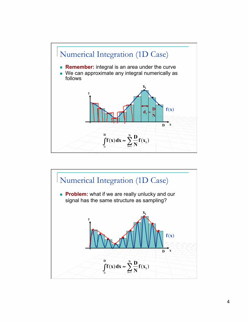
Numerical Integration (1D Case) n Remember: integral is an area under the curve n We can approximate any integral numerically as
follows
x
y
)(xfid
D
∫∑=
∞→⎯⎯ →⎯
DN
iNii dxxfxfd
01)()(
xi
4
Numerical Integration (1D Case) n Remember: integral is an area under the curve n We can approximate any integral numerically as
follows
)(xfNDdi =
D
∑∫=
≈N
ii
D
xfNDdxxf
10
)()(
xi
x
y
Numerical Integration (1D Case)
n Problem: what if we are really unlucky and our signal has the same structure as sampling?
)(xf
D
∑∫=
≈N
ii
D
xfNDdxxf
10
)()(
xi
x
y
5
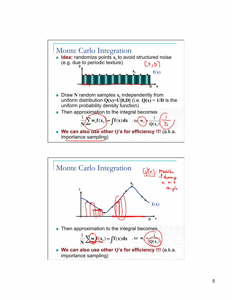
Monte Carlo Integration n Idea: randomize points xi to avoid structured noise
(e.g. due to periodic texture)
n Draw N random samples xi independently from uniform distribution Q(x)=U[0,D] (i.e. Q(x) = 1/D is the uniform probability density function)
n Then approximation to the integral becomes
n We can also use other Q’s for efficiency !!! (a.k.a. importance sampling)
x
y
)(xfxi
D
∑ ∫≈ dxxfxfwN ii )()(1
)(1
ii xQ
w =, for
Monte Carlo Integration
)(xf
D
xi
n Then approximation to the integral becomes
n We can also use other Q’s for efficiency !!! (a.k.a. importance sampling)
∑ ∫≈ dxxfxfwN ii )()(1
)(1
ii xQ
w =, for
x
y

6
n Idea: combination of uniform sampling plus random jitter
n Break domain into T intervals of widths dt and Nt samples in interval t
n Integral approximated using the following:
Stratified Sampling
)(xf
D
∑ ∑= =
T
tjt
N
jt
t
xfdN
t
1,
1)(1
x
y dt
Stratified Sampling n If intervals are uniform dt = D/T and there are same
number of samples in each interval Nt = N/T then this approximation reduces to:
n The interval size and the # of samples can vary !!!
n Integral approximated using the following:
∑ ∑= =
T
tjt
N
jt
t
xfdN
t
1,
1)(1
∑∑= =
T
tjt
N
jxf
NDt
1,
1)(
)(xf
D x
y dt

7
Back to Distribution Ray Tracing n Based on one of the approximate integration approaches
we need to compute q Let’s try uniform sampling
( ) ( )( ) φθθθφθφθφρπφ πθ
dddndpLdddpL iiiee ∫ ∫∈ ∈
⋅−=]2,0[ ]2/,0[
sin),(),(,),(,),(
( ) ( )( ) φθθθφθφθφρ ΔΔ⋅−≈∑∑= =
sin),(),(,),(,1 1
M
m
N
nnminminmie dndpLdd
N
Mπ
φ
πθ
2
2/
=Δ
=Δ
φφ
θθ
Δ⎟⎠
⎞⎜⎝
⎛ −=
Δ⎟⎠
⎞⎜⎝
⎛ −=
2121
m
n
m
n
where
midpoint of the interval (sample point) Interval width
Importance Sampling in Distribution Ray Tracing n Problem: Uniform sampling is too expensive (e.g.
100 samples/hemisphere with depth of ray recursion of 4 => 1004=108 samples per pixel … with 105 pixels =>1015 samples)
n Solution: Sample more densely (using importance sampling) where we know that effects will be most significant q Direction toward point or extended light source are
significant q Specular and off-axis specular are significant q Texture/lightness gradients are significant q Sample less with greater depth of recursion
8
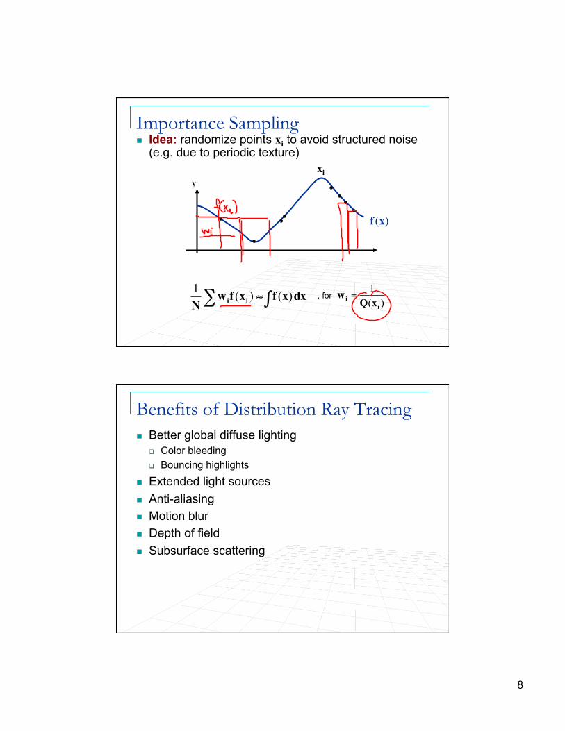
Importance Sampling n Idea: randomize points xi to avoid structured noise
(e.g. due to periodic texture)
∑ ∫≈ dxxfxfwN ii )()(1
)(1
ii xQ
w =, for
)(xf
xi y
Benefits of Distribution Ray Tracing n Better global diffuse lighting
q Color bleeding q Bouncing highlights
n Extended light sources n Anti-aliasing n Motion blur n Depth of field n Subsurface scattering

9
Shadows in Ray Tracing n Recall, we shoot a ray towards a light source and
see if it is intercepted
no shadow rays one shadow ray Images from the slides by Durand and Cutler
kn
kp
jik dc ,
−=
l
Anti-aliasing in Distribution Ray Tracer n Lets shoot multiple rays from the same point and attenuate the color
based on how many rays are intercepted
kp
jik dc ,
−=
Images from the slides by Durand and Cutler
l
w/ anti-aliasing
kn
one shadow ray
Same works for anti-aliasing of
Textures !!!
10
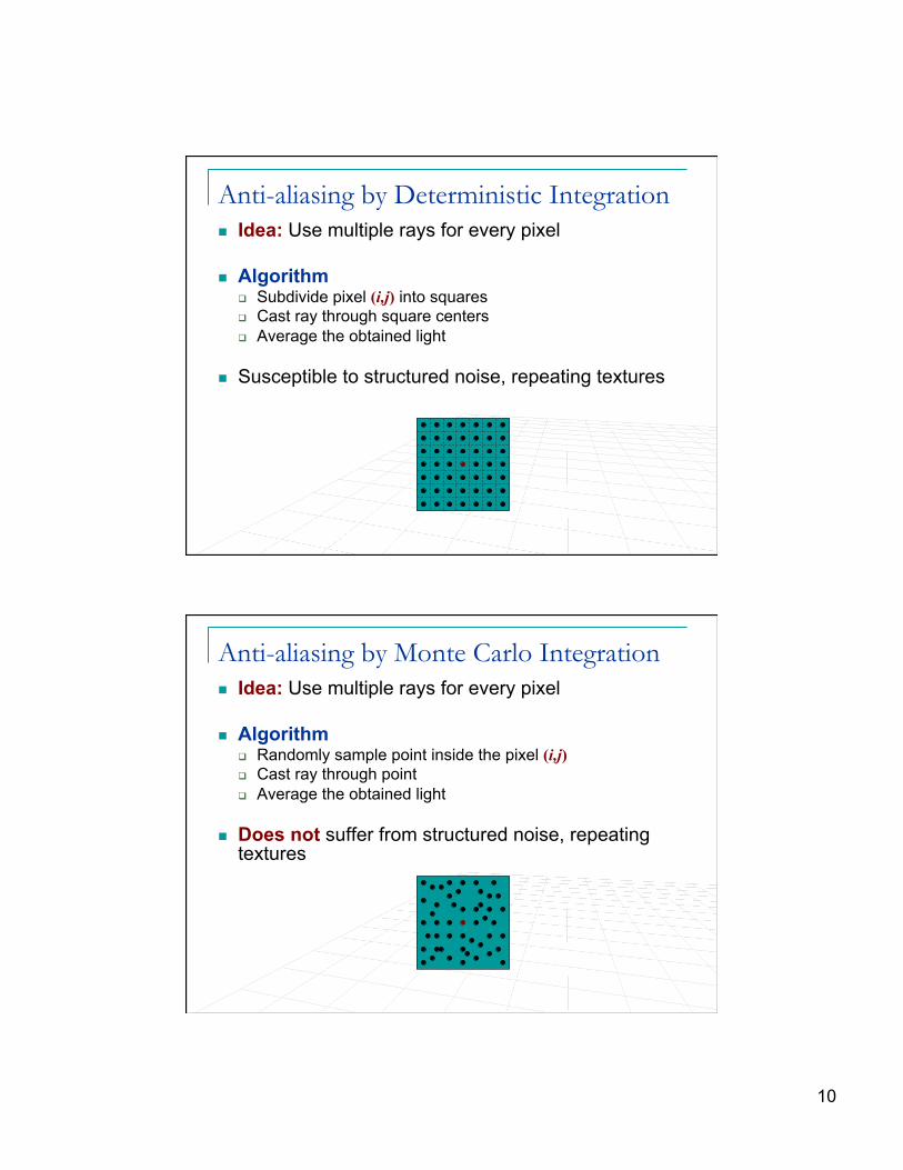
Anti-aliasing by Deterministic Integration n Idea: Use multiple rays for every pixel
n Algorithm q Subdivide pixel (i,j) into squares q Cast ray through square centers q Average the obtained light
n Susceptible to structured noise, repeating textures
Anti-aliasing by Monte Carlo Integration n Idea: Use multiple rays for every pixel
n Algorithm q Randomly sample point inside the pixel (i,j) q Cast ray through point q Average the obtained light
n Does not suffer from structured noise, repeating textures

11
How many rays do you need?
1 ray/light 10 ray/light 20 ray/light 50 ray/light
Images taken from http://web.cs.wpi.edu/~matt/courses/cs563/talks/dist_ray/dist.html
one shadow ray lots of shadow rays
Soft Shadows with Distribution Ray Tracing n Lets shoot multiple rays from the same point and attenuate the color
based on how many rays are intercepted
kn
kp
jik dc ,
−=
Images from the slides by Durand and Cutler

12
Antialiasing – Supersampling
point light
area light
jaggies w/ antialiasing
Images from the slides by Durand and Cutler
Specular Reflections
kn
kp
jik dc ,
−=
ks
kkkkk snnsr −⋅= )(2
kkkks cnncm −⋅= )(2
n Recall, we had to shoot a ray in a perfect specular reflection direction (with respect to the camera) and get the radiance at the resulting hit point

13
Specular Reflections with DRT
kn
kp
jik dc ,
−=
ks
kkkkk snnsr −⋅= )(2
n Same, but shoot multiple rays
Justin Legakis
Spread is dictated by BRDF
Perfect Reflections (Metal)
Perfect Reflections (glossy polished surface)
Depth of Field n So far with our Ray Tracers we only considered
pinhole camera model (no lens) q or alternatively, lens, but tiny aperture
Image Plane Lens
optical axis

14
Depth of Field n So far with our Ray Tracers we only considered
pinhole camera model (no lens) q or alternatively, lens, but tiny aperture
n What happens if we put a lens into our “camera” q or increase the aperture
n Remember the thin lens equation?
Image Plane Lens
optical axis
0z
10
111zzf
+=
1z
Depth of Field n So far with our Ray Tracers we only considered
pinhole camera model (no lens) q or alternatively, lens, but tiny aperture
n What happens if we put a lens into our “camera” q or increase the aperture
n Remember the thin lens equation?
Image Plane Lens
optical axis
0z
10
111zzf
+=
1z

15
Changing the focal-length in DRT
optical axis
0z 1z
220x400 pixels 144 samples per pixel ~4.5 minutes to render
increasing focal length
Changing the aperture in DRT
optical axis
0z 1z
220x400 pixels 144 samples per pixel ~4.5 minutes to render
decreasing aperture

16
Depth of Field
Depth of Field

17
Depth of Field
Depth of Field

18
Depth of Field
Camera Shutter
n We ignored the fact that it takes time to form the image q We ignored this for radiometry
n During that time the shutter is open and light is collected q We need to integrate temporally, not only spatially
dtddtHt
βαβαα β
),,(∫ ∫ ∫
19
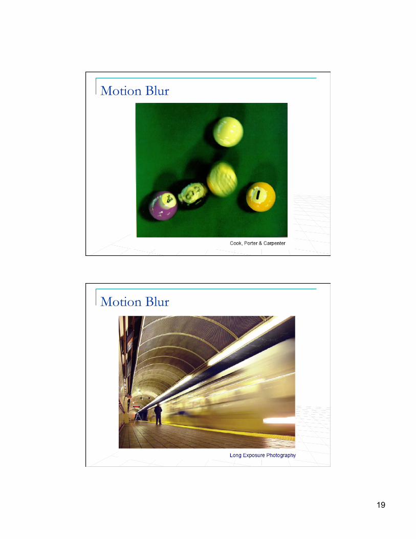
Motion Blur
Motion Blur

20
Motion Blur (long exposures)
Motion Blur (short exposures)

21
Sub-surface Scattering
Sub-surface Scattering Bidirectional Surface Scattering Reflectance Distribution Function

22
Bidirectional Surface Scattering Reflectance Distribution Function
[Images taken from Wikipedia]
Semi-Transparencies
Image form http://www.graphics.cornell.edu/online/tutorial/raytrace/
23
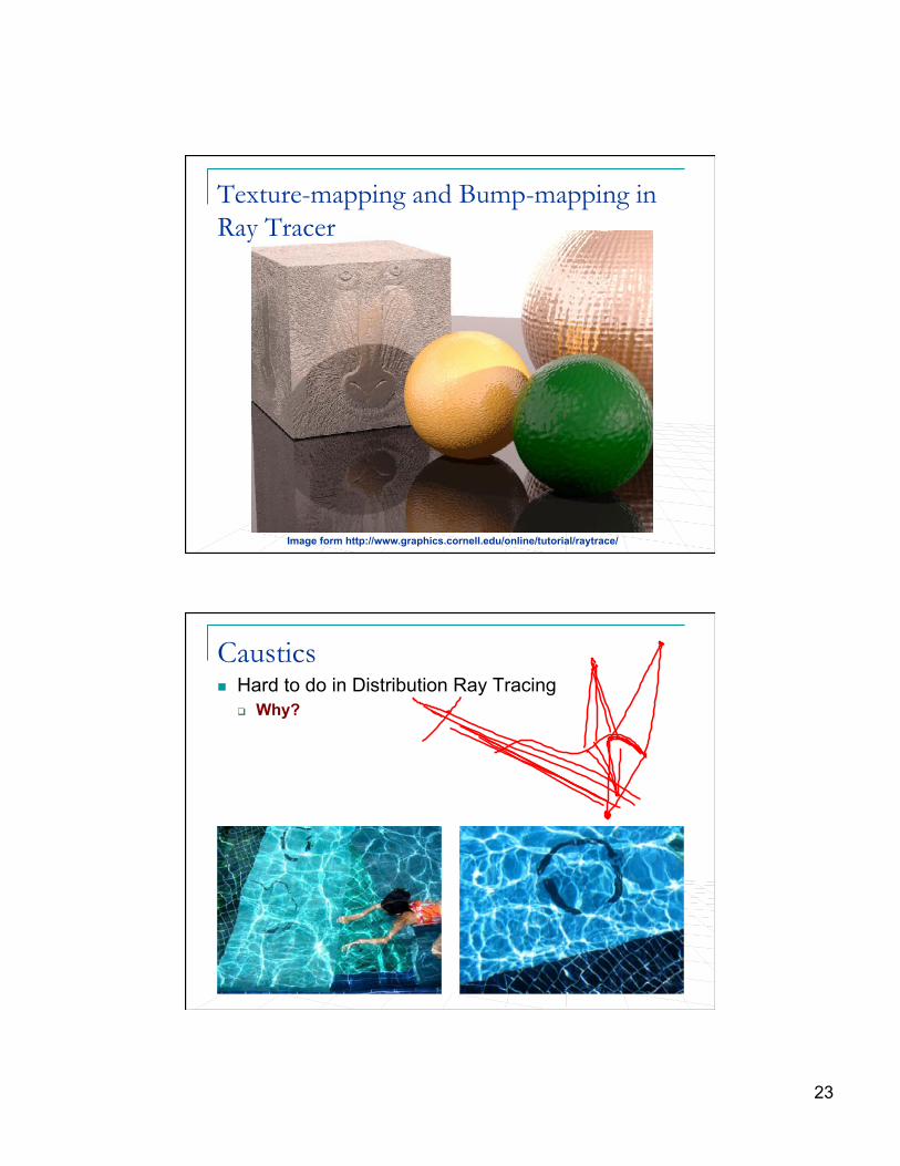
Texture-mapping and Bump-mapping in Ray Tracer
Image form http://www.graphics.cornell.edu/online/tutorial/raytrace/
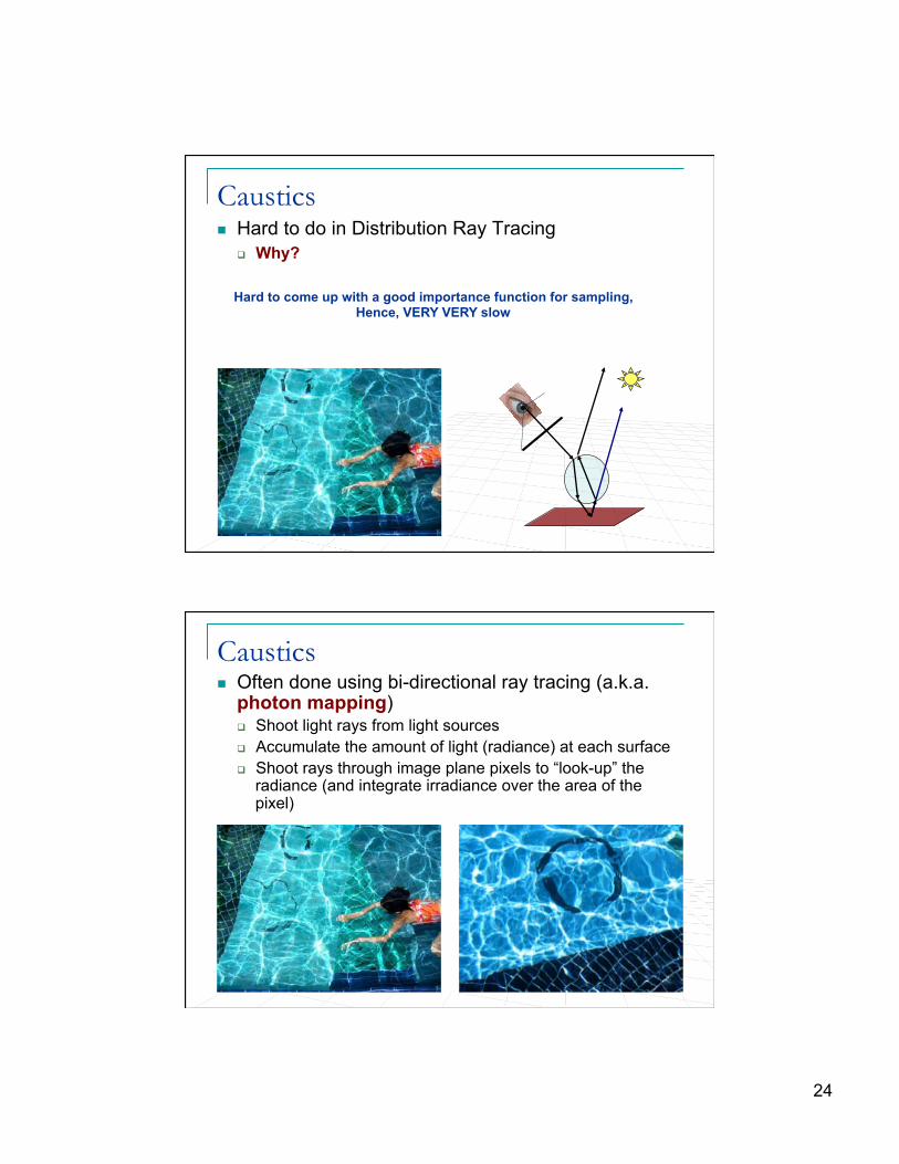
Caustics n Hard to do in Distribution Ray Tracing
q Why?
24
Caustics n Hard to do in Distribution Ray Tracing
q Why?
Hard to come up with a good importance function for sampling, Hence, VERY VERY slow
Caustics n Often done using bi-directional ray tracing (a.k.a.
photon mapping) q Shoot light rays from light sources q Accumulate the amount of light (radiance) at each surface q Shoot rays through image plane pixels to “look-up” the
radiance (and integrate irradiance over the area of the pixel)

25
Photon Mapping
n Simulates individual photons q In DRT we were simulating radiance (flux)
n Photons are emitted from light sources n Photons bounce off of specular surfaces n Photons are deposited on diffuse surfaces
q Held in a 3-D spatial data structure q Surfaces need not be parameterized
n Photons collected by ray tracing from eye
Photons n A photon is a particle of light that carries flux, which
is encoded as follows q magnitude (in Watts) and color of the flux it carries, stored as
an RGB triple q location of the photon (on a diffuse surface) q the incident direction (used to compute irradiance)
n Example (point light source, photons emitted uniformly) q Power of source (in Watts) distributed evenly among photons q Flux of each photon equal to source power divided by total #
of photons q 60W light bulb would sending 100 photons, will result in 0.6
W per photon
26
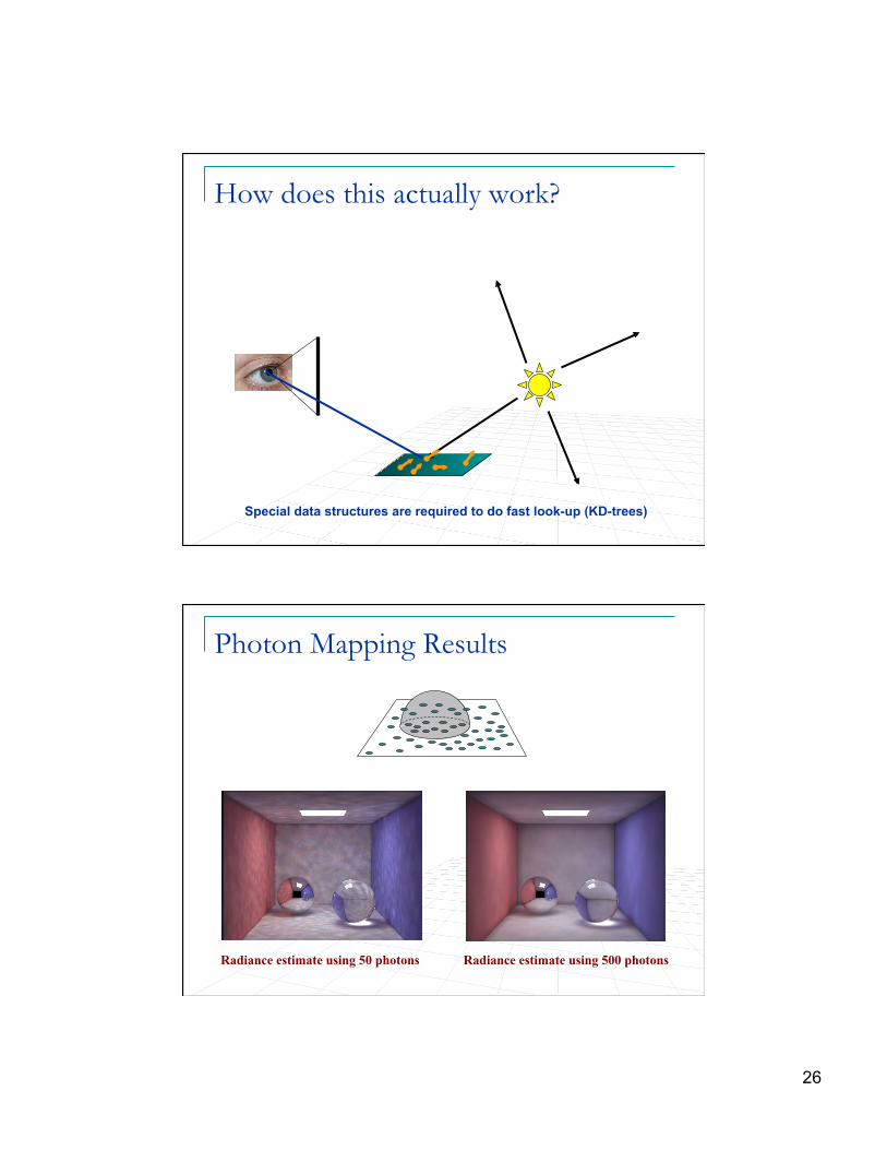
How does this actually work?
Special data structures are required to do fast look-up (KD-trees)
Photon Mapping Results
Radiance estimate using 50 photons Radiance estimate using 500 photons