topics in modeling uncertainty with learning - project...
TRANSCRIPT

Topics in Modeling Uncertainty with Learning
By
Ankit Jain
A dissertation submitted in partial satisfaction of the
requirements for the degree of
Doctor of Philosophy
in
Industrial Engineering and Operations Research
in the
GRADUATE DIVISION
of the
UNIVERSITY OF CALIFORNIA, BERKELEY
Committee in charge:
Associate Professor Andrew E. B. Lim, Co-ChairEmeritus Professor J. George Shanthikumar, Co-Chair
Associate Professor Martin Wainwright
Spring 2010

Topics in Modeling Uncertainty with Learning
Copyright 2010by
Ankit Jain

1
Abstract
Topics in Modeling Uncertainty with Learning
by
Ankit Jain
Doctor of Philosophy in Industrial Engineering and Operations Research
University of California, Berkeley
Associate Professor Andrew E. B. Lim, Co-ChairEmeritus Professor J. George Shanthikumar, Co-Chair
It is fair to say that in many real world decision problems the underlying models cannotbe accurately represented. Uncertainty in a model may arise due to lack of sufficient datato calibrate the model, non-stationarity, or due to wrong subjective assumptions. Henceoptimization in presence of model uncertainty is a very important issue. In the last fewdecades, there has been a lot of work on finding robust solutions to model uncertaintyin operations research. With advances in the field of convex optimization, many robustoptimization problems are efficiently solvable. Still there are many challenges and openquestions related to model uncertainty, specially when learning is also involved. In thisthesis, we study the following challenges and problems related to model uncertainty withlearning:
First, defining and computing a robust solution to problems with model uncertainty isa challenging task, specially in dynamic optimization problems. Many dynamic problemsare tractable only because the structure of the solutions can be analyzed and therefore thedimension of a solution space can be reduced. It is therefore important to design and studyrobust equivalents of dynamic optimization problems and analyze the structure of robustsolutions.
Second, in many situations the need for robust solution arises because of lack of sufficientdata to calibrate model parameters. It is important to study the properties of traditionalrobust solutions. Are these robust solutions good for decision making in long run as comparedto non-robust solutions? If not, is it possible to design alternative approaches?
Third, it is not possible have robustness to model uncertainty if the attention is re-stricted to a wrong model class. One may use a relatively model free learning and decisionmaking methodology such as reinforcement learning, which can achieve an optimal solutionasymptotically. However, these approaches may take a long time to learn and therefore itis important to look at non-parametric methodologies which can achieve good small sampleperformance.
The main contribution of this thesis can be summarized as follows:

2
1. We study an infinite-time queuing control system, where both arrival and departurerates can be controlled. We consider the case when arrival and departure processescan not be accurately modeled. We prove that a threshold policy is optimal undera max-min robust optimization objective when the uncertainty in the processes ischaracterized by a novel notion of relative entropy. The new notion of relative entropyaccounts for different levels of modeling errors in arrival and departure processes.
2. We perform numerical tests to study the performance of traditional robust optimizationsolutions with learning using past few data points. It is shown that the performance ofa robust solution may even be worse than a classical point estimate based non-robustsolution. We introduce the notion of generalized operational statistics that guaranteesa better solution than a classical solution over a set of uncertain parameters, whileincorporating subjective prior information. We apply operational statistics approachto mean-variance portfolio optimization problem with uncertain mean returns. Weshow that the operational statistics portfolio problem can be efficiently solvable byreformulating it as a semi-definite program. Various extensions are discussed andnumerical experiments are done to show the efficacy of the solution.
3. We introduce objective operational learning, a new non-parametric approach that in-corporates structural information to improve small sample performance. We show howstructural and objective information can be incorporated in the objective operationallearning algorithm. We apply the algorithm to an inventory control problem withdemand dependent on inventory level and prove convergence.

i
To my family and friends

ii
Contents
List of Figures iv
List of Tables vi
1 Introduction 1
2 Application of Dynamic Robust Optimization in Queueing Control 62.1 Model Formulation . . . . . . . . . . . . . . . . . . . . . . . . . . . . . . . . 7
2.1.1 Nominal Model . . . . . . . . . . . . . . . . . . . . . . . . . . . . . . 72.1.2 Robust Model . . . . . . . . . . . . . . . . . . . . . . . . . . . . . . . 92.1.3 Relative Entropy . . . . . . . . . . . . . . . . . . . . . . . . . . . . . 10
2.2 Characterization of Optimal Policy . . . . . . . . . . . . . . . . . . . . . . . 122.3 Effect of Ambiguity Parameter on Threshold Control . . . . . . . . . . . . . 20
3 Comparison of Different Approaches to Model Uncertainty with Learning 233.1 Classical Modeling . . . . . . . . . . . . . . . . . . . . . . . . . . . . . . . . 25
3.1.1 Deterministic Modeling . . . . . . . . . . . . . . . . . . . . . . . . . . 253.1.2 Stochastic Modeling . . . . . . . . . . . . . . . . . . . . . . . . . . . 26
3.2 Modeling Errors . . . . . . . . . . . . . . . . . . . . . . . . . . . . . . . . . . 293.2.1 Calibration Error . . . . . . . . . . . . . . . . . . . . . . . . . . . . . 293.2.2 Error due to Wrong Statistical Assumptions . . . . . . . . . . . . . . 31
3.3 Flexible Modeling using Variable Uncertainty set . . . . . . . . . . . . . . . 323.3.1 Deterministic Variable Uncertainty Set . . . . . . . . . . . . . . . . . 343.3.2 Parametric Variable Uncertainty Set . . . . . . . . . . . . . . . . . . 343.3.3 Nonparametric Variable Uncertainty Set . . . . . . . . . . . . . . . . 35
3.4 Robust Optimization Models . . . . . . . . . . . . . . . . . . . . . . . . . . . 373.4.1 Max-min Objective . . . . . . . . . . . . . . . . . . . . . . . . . . . . 373.4.2 Min-max Regret . . . . . . . . . . . . . . . . . . . . . . . . . . . . . . 413.4.3 Max-min Competitive Ratio . . . . . . . . . . . . . . . . . . . . . . . 46
3.5 Learning . . . . . . . . . . . . . . . . . . . . . . . . . . . . . . . . . . . . . . 503.5.1 Reinforcement Learning . . . . . . . . . . . . . . . . . . . . . . . . . 503.5.2 Objective Bayesian . . . . . . . . . . . . . . . . . . . . . . . . . . . . 50
iii
3.5.3 Classical Decision Theory . . . . . . . . . . . . . . . . . . . . . . . . 523.6 Discussion . . . . . . . . . . . . . . . . . . . . . . . . . . . . . . . . . . . . . 53
4 Operational Statistics 544.1 Operational Statistics . . . . . . . . . . . . . . . . . . . . . . . . . . . . . . . 54
4.1.1 Generalized Operational Statistics . . . . . . . . . . . . . . . . . . . . 57
5 Application of Operational Statistics to Portfolio Optimization 605.1 Mean-Variance Portfolio Optimization . . . . . . . . . . . . . . . . . . . . . 605.2 Robust Optimization Approach . . . . . . . . . . . . . . . . . . . . . . . . . 635.3 Operational Statistics Approach to Portfolio Optimization . . . . . . . . . . 635.4 Related Literature . . . . . . . . . . . . . . . . . . . . . . . . . . . . . . . . 695.5 Connection to Norm-Constrained Portfolio . . . . . . . . . . . . . . . . . . . 705.6 Extensions . . . . . . . . . . . . . . . . . . . . . . . . . . . . . . . . . . . . . 71
5.6.1 Using a Prior . . . . . . . . . . . . . . . . . . . . . . . . . . . . . . . 715.6.2 Portfolio with No Risk-Free Asset . . . . . . . . . . . . . . . . . . . . 74
5.7 Numerical Results . . . . . . . . . . . . . . . . . . . . . . . . . . . . . . . . . 75
6 Objective Operational Learning 786.1 Related Literature . . . . . . . . . . . . . . . . . . . . . . . . . . . . . . . . 796.2 Problem Description . . . . . . . . . . . . . . . . . . . . . . . . . . . . . . . 806.3 Non-Parametric Regression . . . . . . . . . . . . . . . . . . . . . . . . . . . . 816.4 Objective Operational Learning . . . . . . . . . . . . . . . . . . . . . . . . . 82
6.4.1 Constructing the Structural model: Newsvendor problem with Observ-able Demand . . . . . . . . . . . . . . . . . . . . . . . . . . . . . . . 82
6.4.2 Summary: Objective Operational Learning . . . . . . . . . . . . . . . 856.5 Application of Objective Operational Learning to Inventory Dependent De-
mand Problem . . . . . . . . . . . . . . . . . . . . . . . . . . . . . . . . . . 87
7 Conclusion 92
Bibliography 94

iv
List of Figures
1.1 Ellsberg Paradox . . . . . . . . . . . . . . . . . . . . . . . . . . . . . . . . . 1
2.1 Queuing System . . . . . . . . . . . . . . . . . . . . . . . . . . . . . . . . . . 72.2 Threshold control variation with ambiguity levels. . . . . . . . . . . . . . . . 222.3 Threshold is increasing if θA = θD . . . . . . . . . . . . . . . . . . . . . . . . 22
3.1 Comparison of classical modeling methods discussed in Section 3.1. Values ofparameters are s=5, c=1, θ = 1. . . . . . . . . . . . . . . . . . . . . . . . . . 30
3.2 Effect of wrong model on long run profit. Demand is gamma distributed withscale parameter 0.1 and shape parameter 10 instead of exponential. . . . . . 32
3.3 Spiral down effect observed using censored demands . . . . . . . . . . . . . . 333.4 Performance of Max-min robust optimization objective with deterministic un-
certainty set. . . . . . . . . . . . . . . . . . . . . . . . . . . . . . . . . . . . 383.5 Sesitivity of Max-min robust optimization (with deterministic uncertainty set)
objective with respect to α . . . . . . . . . . . . . . . . . . . . . . . . . . . . 393.6 Performance of Max-min robust optimization with parametric uncertainty set 403.7 Performance of Max-min robust optimization with non-parametric uncer-
tainty set . . . . . . . . . . . . . . . . . . . . . . . . . . . . . . . . . . . . . 423.8 Performance of of Min-max regret optimization with deterministic uncertainty
set . . . . . . . . . . . . . . . . . . . . . . . . . . . . . . . . . . . . . . . . . 433.9 Sensitivity of Min-max regret optimization (with deterministic uncertainty
set) with α. . . . . . . . . . . . . . . . . . . . . . . . . . . . . . . . . . . . . 443.10 Performance of of Min-max regret optimization with parametric uncertainty set 453.11 Performance of Min-max Regret optimization with non-parametric uncer-
tainty set . . . . . . . . . . . . . . . . . . . . . . . . . . . . . . . . . . . . . 463.12 Performance of Max-min competitive ratio optimization with deterministic
uncertainty set . . . . . . . . . . . . . . . . . . . . . . . . . . . . . . . . . . 483.13 Sensitivity of Max-min competitive ratio optimization (with deterministic un-
certainty set) with α. . . . . . . . . . . . . . . . . . . . . . . . . . . . . . . . 483.14 Performance of Max-min competitive ratio optimization with parametric un-
certainty set . . . . . . . . . . . . . . . . . . . . . . . . . . . . . . . . . . . . 49

v
4.1 Operational statistics policy is uniformly better than the sample mean basedpolicy for newsvendor problem . . . . . . . . . . . . . . . . . . . . . . . . . . 57
5.1 Variation of confidence interval with number of years. It takes many years ofdata to obtain a reasonable estimate of mean of a stock. . . . . . . . . . . . 61
6.1 Comparison of Nadaraya-Watson regression approximation and objective op-erational statistics after two data points . . . . . . . . . . . . . . . . . . . . 85

vi
List of Tables
5.1 Comparison of utilities of operational statistics policy, worst case robust op-timization policy and sample mean based policy . . . . . . . . . . . . . . . . 77

vii
Acknowledgments
My sincere and heartfelt gratitude to all those who have helped and inspired me duringmy doctoral studies.
First and foremost, I like to thank my PhD adviser and dissertation committee chairProf. Andrew Lim for all the support he has given to me over the years. Due to his friendlyand caring attitude it was great fun working with him. His dedication and enthusiasm havealways inspired me to work harder.
I am very grateful to my co-adviser and dissertation committee member Prof. GeorgeShanthikumar for his valuable ideas and insights. I thank him for patiently listening to meduring our meetings and presentations. Without his vision and continual encouragement,the thesis work would not have been possible.
I am grateful to my dissertation committee member Prof. Martin Wainwright for hisvaluable comments during my dissertation workshop and also for his critical comments thatimproved the written presentation of my thesis.
I thank all the past and present members of my research group, Thaisiri Watewai, PengLi, Lian Yu, Gah-Yi Vahn, Sea Chen, Poomyos Fook, Vivek Ramamurthy and HuanningCai, for their helpful remarks during various group presentations.
I also thank all the instructors and GSIs of the courses I have taken. I like to speciallythank Prof. David Aldous, Prof. Jim Pitman, Dr. Shankar Bhamidi, Prof. Michael Jordan,Prof. Peter Bartlett, Prof. Alper Atamturk and Prof. Xin Guo for enriching the technicalskills required for the dissertation work.
I express thanks to my friends and colleagues, Dr. Vishnu Narayanan, Dr. Rahul Tandra,Dr. Ambuj Tewari, Dr. Ismail Ceylan, Dr. Ismail Onur Filiz, Engin Alper, Erick Moreno-Centeno and Sehzad Wadalawala, for many useful discussions and remarks. I also like tothank the IEOR social club, specially Kory Hedman and Stella So, for organizing varioussocial activities and making my stay fun.
I am grateful to all the members of the IEOR administrative staff, specially Mike Camp-bell, Anayancy Paz and Jay Sparks, for their administrative support.
I thank my mentors during my internships at IBM T. J. Watson research, Dr. CathyXia and Dr. Zhen Liu, for their valuable comments on my work, and for providing meopportunities to apply my research in broader areas.
I express my gratitude to all the attendees of my presentations at IEOR student seminars,INFORMS annual meetings and IBM research center for attentively listening to me andproviding valuable feedback.
I thank all my friends and roommates at Berkeley, specially Puneet Bhargava, GautamGupta, Pankaj Kalra, Anurag Gupta and Shariq Rizvi, for making my stay at Berkeley apleasant experience.
I express my sincere gratitude to all the researchers on whose work I am able to buildupon and write this dissertation.
I thank my parents and all other family members for their unconditional love, support

viii
and encouragement. I am very grateful to my brother Ankur Jain for always encouragingand motivating me whenever I was feeling low.
Last but not the least, a very special thanks to Shrutivandana Sharma, without hersupport it would not have been possible to complete the dissertation.

1
Chapter 1
Introduction
In 1961, Daniel Ellsberg described in his work [Ell61], what is commonly known asEllsberg Paradox. An example of the Ellsberg paradox is as follows: there are two urnscontaining red and black balls, from one of which a ball will be drawn at random. Let R2
denotes the choice of betting on red ball from urn 2. Given the choice one will receive $1, ifthe ball drawn is red and $0, if the ball drawn is black. We define the choices R1, B2, B1 andthe associated rewards in a similar way. Now suppose we have the following information:urn 2 contains 100 red and black balls but in a ratio that is unknown and urn 1 contains 50red and 50 black balls. Given this information people are asked to draw their preferences.
It has been observed that most of the people have the following preference:
R1 ⋍ B1 ≻ B2 ⋍ R2, (1.1)
i.e., people are indifferent between R1 and B1 but prefer B1 or R1 over B2 or R2. Anobserver applying the basic rules of probability and utility theory would infer tentativelythat a subject regards the event ‘black from urn 1’ as more likely than ‘black from urn 2’.She would also infer that ‘red from urn 1’ is preferred over ‘red from urn 2’. Since she cannot
100+
?
?
50
50=
=
= =
=
URN 1 URN 2
Figure 1.1: Ellsberg Paradox

2
conclude that ‘red from urn 1’ is more likely than ‘red from urn 2’ and at the same time‘not-red from urn 1’ is more likely than ‘not-red from urn 2’, this behavior is inconsistentwith the essential properties of probability relationships. There is no probability measureon the balls in the urn which supports the preferences described in (1.1).
A probable explanation of people’s behavior in the above example is as follows: in case ofurn 2, the subject has too little information to form a probability distribution (prior) on thenumber of red balls and black balls. Hence she considers a set of possible priors, and beinguncertainty/ambiguity averse she calculates the minimal expected utility over all priors inher subjective uncertainty set while evaluating a bet. To explain the Ellsberg paradox usingthis logic, one may consider the extreme case in which the decision maker takes into accountall possible priors over red and black balls in urn 2. In that case the minimal expected utilityof the choice R2 or B2 is 0 as there is a prior which corresponds to all red balls or all blackballs. On the other hand the minimal expected utility of the choice R1 or B1 is 50 as theexact prior is known. This explains the behavior observed in (1.1). This type of observedbehavior in people’s preferences is also called ambiguity aversion.
The notion of ambiguity or model uncertainty as separate from risk (that can be charac-terized by a probability distribution) was defined as early as 1921 by Frank Knight [Kni21].Over the years ambiguity averse modeling has been studied in many optimization settings byresearchers in the field of operations research (OR). One of the earliest papers in inventorycontrol that considered ambiguity averse modeling was by Scarf [H58] in 1958. He useda min-max objective to find the optimal inventory control policy with unknown demanddistribution, assuming only the precise knowledge of first two moments of the distribution.Gallego and Moon [GM94] extended the model of Scarf to several other cases such as inven-tory control with fixed ordering cost. Advances in the field of convex optimization [Wri97] inlast three decades made it possible to solve ambiguity averse or robust problems, specially inthe field of deterministic optimization, where the parameters (such as product ordering costin an inventory control) of a decision problem are assumed to be uncertain (as opposed tobeing random). Typically these uncertain parameters are assumed to lie in a closed convexregion like an ellipsoid or intervals. If an optimization problem with known parameters isgiven by:
maxx
f(x, (a))
subject to
g(x, b) ≥ 0,
(1.2)
then a robust version of the problem is:
maxx
mina∈A,b∈B
f(x,a)
subject to
g(x, b) ≥ 0, ∀b ∈ B,
(1.3)

3
where x is the decision variable and a, b are parameters of the system. A and B are parameteruncertainty sets in the robust problem for a and b respectively.
For many classes of functions f and g and uncertainty sets, including linear functionsand ellipsoidal uncertainty sets, the robust problem is a “nice” convex program that can beefficiently solved. Some of the works in operations research along this line can be found inBen-Tal and Nemirovski [BTN98, BTN99, BTN00], El Ghaoui and Lebret [EL97], Bertsi-mas and Sim [BS04], Bertsimas and Theile [BTar], El Ghaoui, Oks and Oustry [EOO03],Goldfarb and Iyengar [GI03]. In place of ‘max-min’, alternative objectives such as ‘min-maxregret’ or ‘competitive ratio’ are used too. We study different objectives and their effect onoptimization problems in Chapter 3.
Despite the advances, there has been comparatively little research in OR on robust or am-biguity averse dynamic optimization problems, where state of the world changes with time,mainly because of hardness of resulting dynamic programs. Nilim and El Ghaoui [Nl05]explored robust stochastic dynamic programs where state of the world evolves according toan uncertain probability transition matrix. Their work is closely related to earlier work ineconomics by Epstein and Wang [EW94] and Chen and Epstein [CE02]. Lim and Shan-thikumar [LS07] considered a dynamic pricing problem where uncertainty in probabilitydistribution of future states is characterized by a set of probability distributions which areat a certain “distance” to a nominal probability measure characterized by relative entropy.
In Chapter 2, we consider a dynamic optimization problem of controlling a single stagequeuing system where arrivals and departures are modeled by point processes with stochasticintensities. An arrival incurs a cost while a departure earns a revenue. The objective is tomaximize the profit by controlling the intensities subject to capacity limits and holding costs.When the stochastic model for arrival and departure processes are completely known, thena threshold policy is known to be optimal. We prove that a threshold policy is optimalunder a max-min robust model, when the uncertainty in the processes is characterized byrelative entropy. Our model generalizes the standard notion of relative entropy to accountfor different levels of model uncertainty in arrival and departure processes. Despite thecriticism of max-min model (see Chapter 3) for being too conservative or being too sensitivewith respect to the size of uncertainty set, max-min optimization remains an important toolin robustness and sensitivity analysis. First, it provides a class of policies parametrizedby the size of uncertainty set, which a decision maker can choose from. Second, it is animportant tool to analyze the effect of uncertainty on the decision. For example, in thequeuing problem in Chapter 2, there are problem instances for which the controls are notaffected by uncertainty in arrivals or departures.
Coming back to the discussion on the Ellsberg paradox and ambiguity modeling, oneshould be careful in applying the same concepts when there is repeated decision making andlearning is involved. For example, if one is asked to play the same game as described bythe Ellsberg paradox repeatedly, one can choose a red ball and a black ball alternativelyfrom urn 2 and get the same utility as someone choosing a black or red ball from urn 1.Typically in many operations research problems, the uncertainty is due to lack of sufficient

4
data to learn the parameters of the underlying distribution, non-stationarity in the stochas-tic process or wrong model assumptions. In classical modeling one tends to disregard theuncertainty in estimates of parameters or estimated distribution. It is also common to usethe uncertainty sets estimated from the data, such as confidence intervals or ellipsoids, inrobust optimization problems. it is not clear that if the decisions are made repeatedly, thenthe long run performance of robust models would be better than the classical ones. It is alsoimportant to know how much sensitive the robust models are to the size of uncertainty sets.These issues are explored in detail in Chapter 3.
Even when one is reasonably sure that the true parameter lies in an uncertainty set, itcan not be guaranteed that the robust policy would outperform the classical policy. Ideally,instead of doing optimization and estimation separately, we want a mapping of past datato a policy which is optimal in some way, or is at least better than the classical policy inexpected sense. This in theory may be achieved by defining the negative of objective functionof the problem as a risk function and looking for an estimate which is uniformly betterthan the classical estimate. Unfortunately for many objective functions and distributions ofunderlying stochastic process a uniformly better estimate is impossible or hard to find.
In Chapter 4, we use a novel approach called Operational Statistics which aims to improveon a classical policy (in long run or expected sense) over a set of parameters. This is achievedby explicitly constraining the policy to be better than the classical policy over the set. Theoperational statistics formulation also incorporates subjective information (which may notnecessarily be derived from data) about the underlying parameter. Thus, an operationalstatistics approach would strive to improve on the classical estimation based policy over theuncertainty set while also incorporating subjective belief about the underlying parameter ofthe stochastic process.
In Chapter 5, we apply the operational statistics approach to a mean-variance portfoliooptimization problem with uncertain mean returns of stocks. Given mean return of stocksand covariance matrix, the objective of a mean-variance portfolio optimization problem in-troduced by Markowitz [Mar52] is to find the proportion of different stocks in the portfolio bymaximizing a quadratic utility, which is equal to the average return of portfolio - variance ofthe portfolio multiplied by a risk aversion constant. Estimate of means from limited numberof samples is known to be bad and the policy which replaces actual mean vector with samplemean vector is nown to perform bad out of sample. We show that our operational statisticsmean variance portfolio optimization problem can be reformulated as a semi-definite pro-gram and thus can be solved reasonably efficiently. We show the connection of our approachwith norm constrained portfolio optimization approach and discuss various extensions andnumerical experiments.
Another important issue in repeated decision making, which involves repeated estima-tion and optimization steps, is the effect of optimization step on estimation, particularlyif the model assumptions are wrong. It has been observed in revenue management prob-lems [CdMK06] that using inaccurate model assumptions may lead to progressively worseestimates and in turn worse per step revenue. One simple example of such a phenomenon is
5
the case of censored demand. Suppose someone is observing demand for a particular productby observing how many units of that particular product are sold on a retail store shelf. Thatperson does not realize that the demand she observes in a particular period is the minimumof the actual demand and number of units on the shelf. In a stochastic demand setting theoptimal number of units to order or place on shelf (see Chapter 3) is a particular quantileof the demand distribution. So if use quantiles of empirical distribution constructed fromsales data, it may so happen that we may progressively have worse quantiles, and thus inturn have progressively worse “optimal” order quantity. This results in a per step revenuefunction that spiral down to zero. In general such a situation may arise when demand isdependent on existing inventory or in many pricing problems.
In presence of inaccurate model assumptions, one may be tempted to use a relativelymodel free approach like reinforcement learning [SB98] or multi-arm bandits [ACBF02].However, there is more structural information available than what is typically used in amulti-arm bandit algorithm. For example, given the demand in a particular period andorder quantity we know the exact functional form of profit function. Ignoring these structuralinformation may lead to poor small sample performance. In Chapter 6 we introduce a newapproach called Objective Operational Learning which utilizes this information efficiently.We apply the approach to an inventory control problem with demand dependent on inventorylevel. We show the comparison of objective operational learning approach to non-parametricregression and prove asymptotic convergence.

6
Chapter 2
Application of Dynamic RobustOptimization in Queueing Control
We consider a general single-stage queuing system, in which the input (arrival) and output(service completion) processes are modeled by point processes with dynamically controlledstochastic intensities. An entering job incurs a cost, c, and a job completion producesrevenue, p. In addition there is a holding cost which is linearly proportional to the numberof jobs in the system at a given time. The problem is to dynamically control both the inputand output intensities so as to maximize discounted profit.
Problems of this type have been studied for example by Chen and Yao [CY90], where itis shown that a threshold policy for both the input and output processes is optimal underthe assumption that the stochastic model for arrival and departure processes is accurate andknown. (See the papers [Li88], [Sti85] and [Ser81] for similar results). In many applications,however, arrival and departure intensities can not be accurately modeled due to complexitiesof the real-world system or lack of sufficient calibration data. This raises natural questionsincluding (i) what is the impact of model uncertainty on the “optimal” operating policies forthe system, and (ii) are threshold policies still “optimal”? We account for model errors byformulating a max-min robust control version of this problem in which model uncertaintyis incorporated using the notion of relative entropy. Within this framework, we show thatthreshold policy is optimal for the robust control problem, and study the impact of the levelof model uncertainty on the optimal threshold level.
While the use of relative entropy to account for model uncertainty in stochastic opti-mization problems has a relatively long history ( [PJD00], [LS07], [HSTW06] and [PMR96]),one feature of our work which departs from the standard approach is that we generalizethe standard notion of relative entropy in order to allow for different levels of model uncer-tainty for the arrival as well as the departure processes (see also Lim, Shanthikumar andWatewai [LSW09] for similar ideas in the context of dynamic pricing). Aside from beingrealistic–for example, it is likely to be the case that the system operator is substantiallymore knowledgeable about the service system he/she in controlling (since it is internal) than

2.1. MODEL FORMULATION 7
the customer arrival process, which is typically much more complicated and subject to manyexternal factors–this also allows us to study (say) the impact of the level of model uncertaintyin the arrival process on the service control policy.
The outline of this chapter is as follows. In Section 2.1 we recall the model from Chen andYao [CY90] and formulate the robust version of this problem. The robust version involvesan extension of the notion of discounted relative entropy from Hansen, Sargent, Turmuham-betova and Williams [HSTW06] in order to handle different levels of model uncertainty forthe arrival and departure processes. Dynamic programming equations for the robust controlproblem are derived in Section 2.2, and the impact of the level of model uncertainty on thethreshold control levels is studied in Section 2.3.
2.1 Model Formulation
In this section we first introduce the standard model which is similar to [CY90] beforeformulating the robust model in section 2.1.2. The robust model extends the notion ofdiscounted relative entropy from [HSTW06] in order to handle different level of uncertaintiesin arrival and departure rates.
2.1.1 Nominal Model
Consider a single-stage queuing system as shown in Fig. 2.1. Let Xt be the state of thesystem that denotes the number of jobs in process at time t. Xt takes values on nonnegativeintegers and is of the form
Xt = x0 + At −Dt, (2.1)
where x0 ≥ 0 is the state at time t = 0 of the system and At and Dt are the arrival anddeparture processes respectively. At and Dt denote the cumulative number of arrivals anddepartures until time t.
DtAtX t
Figure 2.1: Queuing System
We assume that At and Dt are simple point processes. Let Ft be the sigma field generatedby Xt, i.e., Ft = σ(Xs, s ≤ t). Also let At and Dt admit Ft predictable intensities βt and αt.

2.1. MODEL FORMULATION 8
The rates αt and βt are subjected to the following capacity constraints
0 ≤ βt ≤ y, ∀t ≥ 0, and
0 ≤ αt ≤ z, ∀t ≥ 0.(2.2)
If there is no ambiguity in the arrival or departure process, i.e., if we can exactly controlthe arrival and departure intensities, then our objective is to find a control u = βt, αt, t ≥ 0to maximize the following discounted value function:
V (x0, u) = Ex0
∫ ∞
0
e−δt(pdDt − cdAt − hXtdt). (2.3)
Here Ex0 denotes the conditional expectation given X0 = x0, δ is the discount factor, p is therevenue obtained by selling one unit of output, c is the cost of acquiring one unit of input andh is the unit holding cost for work-in-process inventory. Substituting Xt from (2.1) in (2.3)we obtain:
V (x0, u) = Ex0
∫ ∞
0
e−δt
((
p+h
δ
)
dDt −
(
c+h
δ
)
dAt
)
−hx0
δ. (2.4)
Defining p = p+ hδ
and c = c+ hδ
we have
V (x0, u) = Ex0
∫ ∞
0
e−δt (pdDt − cdAt) −hx0
δ. (2.5)
We can drop the last term in (2.5) for the purpose of finding optimal control as it is aconstant term. From the definition of stochastic intensity [Bre81]
Ex0
∫ ∞
0
cdAt = Ex0
∫ ∞
0
cβtdt,
Ex0
∫ ∞
0
pdDt = Ex0
∫ ∞
0
pαtdt.
(2.6)
Rewriting the value function in (2.5) using (2.6) and dropping the constant term we have
V (x0, u) = Ex0
∫ ∞
0
e−δt (pdDt − cdAt) = Ex0
∫ ∞
0
e−δt (pαt − cβt) dt. (2.7)
The problem formulation with unambiguous arrival rate is:
maxu
V (x0, u) = maxu
Ex0
∫ ∞
0
e−δt (pαt − cβt) dt. (2.8)

2.1. MODEL FORMULATION 9
2.1.2 Robust Model
Let (Ω,Ft,F) be the underlying measurable space for arrival and departure processes,At and Dt respectively. At and Dt are counting processes and admit intensities. A completespecification of intensity λt of the process At and of intensity µt of the process Dt induces ameasure P over F . The nominal model is based on the assumption that the decision makeris able to set arrival and departure intensities precisely subject to capacity constraints. Theobjective then is to find (λt, µt) which are optimal.
In reality the real-world intensity processes are unlikely to be (λt, µt). For example, thearrival rate, λt, might be a function of the price an arriving customer pays for the servicebeing offered while µt could depend on the number of workers assigned to the customer inservice, and the assumption in the nominal model is the decision maker knows the exactrelationship between pricing decisions and the arrival rate λt, as well as the number ofworkers assigned and the departure rate µt, so that the arrival and departure rates can beset to the precise values that the decision maker desires. In practice, the relationship betweenthe pricing decision and λt and also the number of assigned workers and the service rate µt
may be difficult to characterize. The arrival intensity might be a complicated non-stationaryfunction of the price and also of other factors such as amount of advertising. This makes itimpossible to precisely calibrate intensities.
More generally we have a situation where the decision maker on the basis of her modelthinks she is setting the arrival and departure rates at levels (λt, µt) but in reality the ratesmight be something different (say (βt, αt)). Our objective in this section is to incorporatethe possibility of such model uncertainty into the formulation of the problem.
Suppose the real-world Ft-predictable intensity processes βt and αt induces a measureQ over F . We assume that the real-world intensity processes, while not known accurately,satisfy certain minimal conditions with respect to the intensity processes λt and µt, which areprecisely known to the decision maker. Let Pt and Qt be restrictions of P and Q respectivelyto Ft. In particular we assume that for all t, Qt is absolutely continuous with respect to Pt,i.e.,
Pt(A) = 0 ⇒ Qt(A) = 0 ∀A ∈ Ft.
The distribution Q is said to be absolutely continuous over finite intervals with respectto P if Qt is absolutely continuous with respect to Pt for all t. This definition of absolutecontinuity captures the idea that two models are impossible to distinguish with certaintyover a finite interval([HSTW06]).
Let γt, t ≥ 0 be a stochastic process such that for every t, γt is Radon-Nikodymderivative [Dur03] of Qt with respect to Pt. γt is a positive martingale and is adapted tofiltration Ft. It follows from [Jac79] that there are Ft-predictable processes κt and ηt suchthat:
γt = exp
(∫ t
0
(ln(κs)dAs + ln(ηs)dDs) +
∫ t
0
((1 − κs)λs + (1 − ηs)µs) ds
)
(2.9)

2.1. MODEL FORMULATION 10
The following result is a version of the Girsanov Theorem for point processes as stated inBremaud [Bre81].
Theorem 1 (Girsanov Theorem). Let At and Dt be Ft-adapted point processes with Ft-predictable intensities λt and µt respectively under the probability measure P . Suppose thatγt is a positive Ft-martingale under P and that the Radon-Nikodym density of Qt with respectto Pt is given by
dQt
dPt
= γt = exp
(∫ t
0
(ln(κs)dAs + ln(ηs)dDs) +
∫ t
0
((1 − κs)λs + (1 − ηs)µs) ds
)
, (2.10)
then At and Dt are Ft-adapted point processes with intensities βt = κtλt and αt = ηtµt
respectively under Q.
Theorem 1 allows us to parameterize the real-world model Q = (βt, αt, t ≥ 0) throughthe processes κt and ηt.
2.1.3 Relative Entropy
Relative entropy or KL divergence is a measure of difference between two probabilitymeasures. Here we use a weaker notion, called Discounted Relative Entropy [HSTW06] tomeasure the discrepancy between two measures over an infinite horizon.
The weaker notion requires that the two measure being compared put positive probabilityon all of the same events, except tail events. The discounted relative entropy is defined as:
R(Q|P ) = δ
∫ ∞
0
exp(−δt)
(∫
ln
(
dQt
dPt
)
dQt
)
dt, (2.11)
where dQt
dPtis the Radon-Nikodym derivative of Qt with respect to Pt.
This measure of relative entropy is convex in Q as shown in [HSTW06]. It should benoted here even if the discounted measure of entropy is finite the standard relative entropymeasure of distance between P and Q can be infinite, i.e., it allows:
∫
log
(
dQ
dP
)
dQ = +∞ (2.12)
If (2.12) holds but discounted relative entropy (2.11) is finite, then it means that astatistician would be able to distinguish between the probability measures P and Q with acontinuous record of data on an infinite interval while it is impossible to do so by recording afinite length time interval data. As an example if under P the arrival rate is constant λ andunder Q the arrival rate is constant β, β 6= λ, then relative entropy of P and Q is infinitebut the discounted relative entropy between Q and P is finite.

2.1. MODEL FORMULATION 11
Returning to our discussion on point processes, it follows from Theorem 1 that ourmeasure of discounted relative entropy (2.11) transforms into:
R(Q|P ) = δ
∫ ∞
0
e−δt
(∫
lndQt
dPtdQt
)
dt
= δ
∫ ∞
0
e−δt
(∫ t
0
(λs(κs lnκs + 1 − κs) + µs(ηs ln ηs + 1 − ηs)) ds
)
dt
= δ
∫ ∞
0
(λs(κs lnκs + 1 − κs) + µs(ηs ln ηs + 1 − ηs)) ds
(∫ ∞
s
e−δtdt
)
=
∫ ∞
0
e−δsλs(κs lnκs + 1 − κs)ds+
∫ ∞
0
e−δsµs(ηs ln ηs + 1 − ηs)ds.
(2.13)
where the third equality is justified by Fubini’s theorem [Dur03] as the integrand is positive.The first term R1(Q|P ) =
∫∞
0e−δsλs(κs lnκs + 1 − κs)ds can be interpreted as measure of
ambiguity in the arrival process. Similarly the second term R2(Q|P ) =∫∞
0e−δsµs(ηs ln ηs +
1 − ηs)ds measures the ambiguity in the departure process.Our robust control problem corresponding to (2.8) is as follows:
maxu∈U minQ EQ
[∫∞
0e−δt (pαt − cβtdt)
]
subject to: R(Q|P ) ≤ η.(2.14)
Here the control is u = λt, µt, λt ≤ y, µt ≤ z, t ≥ 0.The robust control problem is a two-player game between ‘nature’ and decision maker.
Given the control u, nature chooses a “worst-case” measure Q from the class of measuresdefined by the convex discounted relative entropy constraint. The constant η ≥ 0 is ameasure of our confidence in the nominal measure P and restricts the amount that Q (orthe real-world intensity processes βt and αt) can deviate from P (resp. λt and µt). A largevalue of η allows Q to deviate further from our nominal probability measure P while a smallvalue of η is chosen when we have a high degree of confidence in our nominal model. Puttingη = 0 reduces the robust control problem to a standard one.
Alternatively, we may consider the following problem:
maxu∈U
minQ
(
EQ
[∫ ∞
0
e−δt (pµt − cβtdt)
]
+ θR(Q|P )
)
. (2.15)
The constant θ > 0 may be seen as the Lagrange multiplier for the relative entropy constraintin (2.14) and solving (2.14) is equivalent to solving (2.15) for an appropriate choice of θ.Alternatively, the parameter θ can represents our confidence in the nominal model. A largevalue of θ denotes high confidence in the model as the penalty of deviation from the modelis large.
Note that the discounted relative entropy in (2.13) is the sum of two terms. The terms

2.2. CHARACTERIZATION OF OPTIMAL POLICY 12
individually can be interpreted as measure of uncertainties in arrival and departure processesrespectively. In formulation (2.15) as both the terms in discounted relative entropy expansionare multiplied by the same constant θ, the confidence levels in arrival and departure processesare assumed to be the same. If we have reason to believe in varying levels of confidence inarrival and departure processes the formulation (2.15) can be modified as:
maxu∈U
minQ
(
EQ
[∫ ∞
0
e−δt (pαt − cβtdt)
]
+ θAR1(Q|P ) + θDR2(Q|P )
)
. (2.16)
where θA and θD denotes the confidence in arrival and departure processes respectively .Hence Model (2.16) differs from standard robust model (2.15) that assumes the same levelof uncertainty for all parts of the model.
Substituting the value of discounted relative entropy for point processes from (2.13)to (2.15) our robust formulation is:
maxu∈U
minκ,η
Ex0
[
∫ ∞
0
e−δt(
pηsµs − cκsλs + θAλs(1 − κs + κs lnκs)
+ θDµs(1 − ηs + ηs ln ηs))
ds]
.
(2.17)
2.2 Characterization of Optimal Policy
Suppose we first restrict ourselves to the policies which are Markov in the state (thenumber of items that are currently in service). In other words, we can replace λt and µt
by λ(Xt) and µ(Xt) respectively. Further assume that nature is restricted to choose amonga set of Markovian policy only, i.e., κ and η are only functions of X. In this case theformulation (2.17) reduces to:
maxλ,µ
minκ
Ex0
[
∫ ∞
0
e−δt(
pη(Xs)µ(Xs) − cκ(Xs)λ(Xs) + θAλ(Xs)(1 − κ(Xs)
+ κ(Xs) lnκ(Xs)) + θDµ(Xs)(1 − η(Xs) + η(Xs) ln η(Xs)))
ds]
.
(2.18)
The Hamiltonian-Jacobi-Bellman (HJB) equation corresponding to the above formulationis:
δV (x) = maxλ(x),µ(x)
minκ(x),η(x)
[
λ(x)κ(x)(−c + θA(−1 + lnκ(x)) + ∆V (x)) + λ(x)θA
+ µ(x)η(x)(p+ θD(−1 + ln η(x)) − ∆V (x− 1)) + µ(x)θD
]
,
(2.19)
where∆V (x) = V (x+ 1) − V (x), (2.20)

2.2. CHARACTERIZATION OF OPTIMAL POLICY 13
and
V (x) = maxλ,µ
minκ,η
Ex
[
∫ ∞
0
e−δt(
pµ(Xs) − cκ(Xs)λ(Xs) + θAλ(Xs)(1 − κ(Xs)
+ κ(Xs) lnκ(Xs)) + θDµ(Xs)(1 − η(Xs) + η(Xs) ln η(Xs)))
ds]
.
(2.21)
The solution of the (unconstrained convex) inner minimization (with respect to κ and η)problem in (2.19) is characterized by the first order conditions and yields the following
κ∗(x) = exp
(
−1
θA(∆V (x) − c)
)
, and
η∗(x) = exp
(
−1
θD(p− ∆V (x− 1))
)
.
(2.22)
Substituting back the value of κ∗ and η∗(x) from (2.22) to (2.19), we obtain the followingafter some manipulation:
δV (x) = maxλ(x),µ(x)
[
θAλ(x)(
1 − exp(
−1
θA(∆V (x) − c)
))
+ θDµ(x)
(
1 − exp(−1
θD
(p− ∆V (x− 1))
)
]
.
(2.23)
As the above equation is linear in λ(x) and µ(x), we obtain the following characterizationof the optimal policy
λ∗(x) =
y if ∆V (x) ≥ c0 otherwise.
(2.24)
µ∗(x) =
z if ∆V (x− 1) ≤ p, x ≥ 10 otherwise.
(2.25)
This proves that optimal policy would either allow arrivals at full force or not to allowarrivals at all. The same structure holds for production. We either produce at full force ordo not produce at all. In order to guarantee that the optimal policy is threshold we need toprove the existence of a number b such that:
c ≤ ∆V (x) ≤ p for x ≤ b∆V (x) < c for x > b.
(2.26)
As it does not make sense to stop the production if there is a positive inventory due todiscounting and the holding cost, it is obvious that the optimal output policy should be of

2.2. CHARACTERIZATION OF OPTIMAL POLICY 14
the following form:
µ∗(x) =
z if x ≥ 10 otherwise.
(2.27)
Now consider the following policy for arrivals. At every stage there is a choice betweensetting the arrival intensity to zero or setting it equal to its max value of y. The valuefunction if we follow this binary policy which we have already proved to be optimal in thecase when both nature and decision maker is restricted to the class of Markovian policies is:
V (x) = maxλ(·)∈0,y
Ex
[
∫ ∞
0
e−δt(
pµ∗(Xs)η∗(Xs) − cκ∗(Xs)λ(Xs)
+ θAλ(Xs)(1 − κ∗(Xs) + κ∗(Xs) lnκ∗(Xs))
+ θDµ(Xs)(1 − η∗(Xs) + η∗(Xs) ln η∗(Xs)))
ds]
.
(2.28)
µ∗(x) is as described in (2.27), and κ∗(x), η∗(x) are as in (2.22). Now suppose we canfind a finite constant ν such that ν ≥ (yκ∗(x) + zη∗(x)), ∀x. The existence of such a ν isguaranteed if we look at the expression (2.22) as it is possible to obtain upper and lowerbounds on V (x).1 Given such a ν we can write the following dynamic programming equation( see Bertsekas [Ber95] Ch. 5)
V (x) =1
δ + ν
[
pµ∗(x)η∗(x) + µ∗(x)θD(1 − η∗(x) + η∗(x) ln η∗(x))
+ (ν − µ∗(x))V (x) + µ∗(x)V (x− 1)
+ max(
− cyκ∗(x) + yθA(1 − κ∗(x) + κ∗(x) lnκ∗(x))
+ yκ∗(x)(V (x+ 1) − V (x)), 0)
.
(2.29)
Without loss of generality we can assume that δ+ν = 1 as it is possible to scale upper boundsz and y appropriately. Substituting the value of κ∗(x) and η∗(x) from (2.22) in (2.29) andsimplifying we obtain:
V (x) = µ∗(x)θD
(
1 − e− 1
θD(p−∆V (x−1))
)
+ νV (x) + yθA max(
1 − e− 1
θA(∆V (x)−c)
, 0)
. (2.30)
To prove the structural properties of V (x) consider the following value-iteration algorithm:
Vn+1(x) = µ∗(x)θD
(
1 − e− 1
θD(p−∆Vn(x−1))
)
+ νVn(x) + yθA max(
1 − e− 1
θA(∆Vn(x)−c)
, 0)
.
(2.31)
Such a value-iteration algorithm corresponding to a stochastic game can be shown toconverge to the true value function (see [Sha53]). Note that similar iteration equations are
1Zero is a lower bound. An upper bound is the value function of the unambiguous problem which can be
uniformly upper bounded.

2.2. CHARACTERIZATION OF OPTIMAL POLICY 15
observed in risk sensitive control literature (see [HHM96], [BM02], [CCdO03] and [CM99]).The set of value-iteration equations can be written more explicitly in the following form:
Vn+1(x) = zθD
(
1 − e− 1
θD(p−∆Vn(x−1))
)
+ νVn(x) + yθA max(
1 − e− 1
θA(∆Vn(x)−c)
, 0)
(2.32)
where by convention ∆Vn(−1) = p for all n so that e− 1
θD(p−∆Vn(−1))
= 1.
Theorem 2. Suppose we initialize V0(x) = 0 for all x. If we iterate according to equa-tion (2.32) then the following holds true for every n
(a) ∆Vn(x) ≤ p.
(b) Vn(x) is increasing in x, i.e., ∆Vn(x) ≥ 0.
(c) Vn(x) is concave in x, i.e., ∆Vn(x) is decreasing in x.
Proof. Proof is by induction. By construction the hypothesis holds true for n = 0. We nowsuppose that it holds for n = k and show that it holds for n = k + 1.
(a)
∆Vk+1(x) = zθD
((
(1 − e− 1
θD(p−∆Vk(x))
)
−(
1 − e− 1
θD(p−∆Vk(x−1))
))
+ ν(∆Vk(x))
+ yθA
(
max(1 − e− 1
θA(∆Vk(x+1)−c)
, 0) − max(1 − e− 1
θA(∆Vk(x)−c)
, 0))
≤ zθD
(
1 − e− 1
θD(p−∆Vk(x))
)
+ ν∆Vk(x)
≤ z(p− ∆Vk(x)) + ν∆Vk(x) = zp + (ν − z)p ≤ zp+ (ν − z)p = p.
We have used the following facts: max(1 − e− 1
θA(∆Vk(x+1)−c)
, 0) ≤ max(1 − e− 1
θA(∆Vk(x)−c)
, 0)
as ∆Vk(x) is a decreasing function of x,(
1 − e− 1
θD(p−∆Vk(x−1))
)
≥ 0 as ∆Vk(x − 1) ≤ p for
all x and 1 − e−s ≤ s when x ≥ 0.(b)
∆Vk+1(x) = zθD
(
e− 1
θD(p−∆Vk(x−1))
− e− 1
θD(p−∆Vk(x))
)
+ ν(∆Vk(x))
+ yθA
(
max(1 − e− 1
θA(∆Vk(x+1)−c)
, 0) − max(1 − e− 1
θA(∆Vk(x)−c)
, 0))
≥ ν∆Vk(x) + yθA
(
max(1 − e− 1
θA(∆Vk(x+1)−c)
, 0) − max(1 − e− 1
θA(∆Vk(x)−c)
, 0))
≥ ν∆Vk(x) − yθA max(
1 − e− 1
θA(∆Vk(x)−c)
, 0)
.
If ∆Vk(x) ≤ c, then max(1 − e− 1
θA(∆Vk(x)−c)
, 0) = 0 and hence ∆Vk+1(x) ≥ ν∆Vk(x) ≥ 0.

2.2. CHARACTERIZATION OF OPTIMAL POLICY 16
Else if ∆Vk(x) ≥ c, then
∆Vk+1(x) ≥ ν∆Vk(x) − yθA
(
1 − e− 1
θA(∆Vk(x)−c)
)
≥ ν∆Vk(x) − yθA∆Vk(x) − c
θA
≥ (ν − y)∆Vk(x) ≥ 0.
Here we have used the fact that 1 − e−s ≤ s when s ≥ 0.(c)
∆Vk+1(x) − ∆Vk+1(x+ 1) = zθD
(
e−
f(x−1)θD − 2e
−f(x)θD + e
−f(x+1)
θD
)
+ ν(∆Vk(x) − ∆Vk(x+ 1))
+ yθA(2 max(1 − e− g(x+1)
θA , 0) − max(1 − e− g(x)
θA , 0) − max(1 − e− g(x+2)
θA , 0)),
where f(x) = p − ∆V (x) and g(x) = ∆V (x) − c. Note that as 0 ≤ f(x) ≤ p and f(x) isincreasing in x we have
e−
f(x−1)θD − e
−f(x)θD ≥ 0.
Also as g(x) is decreasing in x,
max(1 − e−
g(x+1)θA , 0) − max(1 − e
−g(x+2)
θA , 0) ≥ 0.
Therefore
∆Vk+1(x) − ∆Vk+1(x+ 1) ≥ zθD
(
e− f(x+1)
θD − e− f(x)
θD
)
+ ν(∆Vk(x) − ∆Vk(x+ 1))
+ yθA
(
max(1 − e− g(x+1)
θA , 0) − max(1 − e− g(x)
θA , 0)
)
= zθD
(
e−
f(x+1)θD − e
−f(x)θD
)
+ z((p− ∆Vk(x+ 1)) − (p− ∆Vk(x)))
+ yθA
(
max(1 − e− g(x+1)
θA , 0) − max(1 − e− g(x)
θA , 0)
)
+ y((∆Vk(x) − c) − (∆Vk(x+ 1) − c))
+ (ν − y − z)(∆Vk(x) − ∆Vk(x+ 1))
≥ zθD
((
e− f(x+1)
θD +f(x+ 1)
θD
)
−
(
e− f(x)
θD +f(x)
θD
))
+ yθA
(
max(1 − e−
g(x+1)θA , 0) −
g(x+ 1)
θA
)
− yθA
(
max(1 − e−
g(x)θA , 0) −
g(x)
θA
)
.

2.2. CHARACTERIZATION OF OPTIMAL POLICY 17
e−s + s is an increasing function of s when s ≥ 0, so
(
e− f(x+1)
θD +f(x+ 1)
θD
)
−
(
e− f(x)
θD +f(x)
θD
)
≥ 0.
Also max(1 − e−s, 0) − s is decreasing in s and as g(x) is a decreasing function of x
(
max(1 − e− g(x+1)
θA , 0) −g(x+ 1)
θA
)
−
(
max(1 − e− g(x)
θA , 0) −g(x)
θA
)
≥ 0.
Therefore,∆Vk+1(x) − ∆Vk+1(x+ 1) ≥ 0.
Hence we have proved here that if we restrict ourselves to the class of Markovian policiesand nature is also restricted to choose Markovian policy to hurt the decision maker then athreshold policy is optimum. Specifically we proved that there exists a threshold b ∈ [0,∞]such that
c ≤ V (x+ 1) − V (x) ≤ p for x ≤ bV (x+ 1) − V (x) < c for x > b
(2.33)
Coupled with (2.24) we have the following policy:
λ∗(x) =
y if x ≤ b0 if x > b
(2.34)
Next we will show that the policy remains optimal even if the nature is free to choose anynon-Markovian policy. Specifically we prove that if we choose threshold policy and natureis free to choose anything, nature would choose Markovian policy to hurt most.
Theorem 3. Suppose we choose the input and output intensities according to the equa-tions (2.34) and (2.25). Suppose we allow “nature”, acting as the adversary, to choose anyarbitrary Ft-predictable processes κt and ηt to hurt the decision maker so that the expectedprofit is minimized. Then nature would choose Markovian policy as given by (2.22), wherethe value function in the equation is the optimal one when both nature and decision makerare allowed to choose only Markovian policies.
Proof. For any given arbitrary processes (κt, ηt), t ≥ 0, suppose we consider a situation wherenature follows (κt, ηt) up to time t and then follows Markovian policy given by (2.22) after

2.2. CHARACTERIZATION OF OPTIMAL POLICY 18
that. The value function associated with this (denoted by Vt) can be expressed as follows:
Vt(x) = Ex
∫ t
0
e−δt(
pµ∗(Xs)ηs − cλ∗(Xs)κs
+ θAλ∗(Xs)(1 − κs + κs lnκs) + θAµ
∗(Xs)(1 − ηs + ηs ln ηs)ds)
+ Ex[e−δtV (Xt)].
(2.35)
To derive the second expectation in above equation consider
∫ t
0
e−δsdV (Xs) = e−δtV (Xt) − V (X(0)) + δ
∫ t
0
e−δsV (Xs)ds. (2.36)
Taking expectation on both sides of the equality, we have
Ex
∫ t
0
e−δsdV (Xs) = Ex[e−δtV (Xt)] − V (x) + Ex
[
δ
∫ t
0
e−δsV (Xs)ds
]
. (2.37)
We can calculate the left most term in the above expression as:
Ex
∫ t
0
eδsdV (Xs) = Ex
∫ t
0
e−δs(
[∆V (Xs)]dAs − [∆V (Xs − 1)]dDs
)
= Ex
∫ t
0
e−δs(
κsλ∗(Xs)∆V (Xs) − ηsµ
∗(Xs)∆V (Xs − 1))
ds.
(2.38)
The first equality follows from the fact that there are only two possible transitions,upward and downward, and the second equality follows from (2.6). From (2.35) and (2.38)we obtain:
Ex[e−δtV (Xt)] = V (x) + Ex
∫ t
0
e−δs(
κsλ∗(Xs)∆V (Xs)
− ηsµ∗(Xs)∆V (Xs − 1) − δV (Xs)
)
ds.
(2.39)
From (2.23) we have
δV (Xs) = θAλ∗(x)
(
1 − exp(
−1
θA
(∆V (Xs) − c)))
+ θDµ∗(x)
(
1 − exp
(
−1
θD
(p− ∆V (Xs − 1))
))
.(2.40)
2.2. CHARACTERIZATION OF OPTIMAL POLICY 19
From (2.39) and (2.40) we obtain
Ex[e−δtV (Xt)] = V (x) + Ex
∫ t
0
e−δs(
κsλ∗(Xs)∆V (Xs) − ηsµ
∗(Xs)∆V (Xs − 1))
ds
−Ex
∫ t
0
e−δsθAλ∗(x)
(
1 − exp(
−1
θA
(∆V (Xs) − c)))
ds
+ Ex
∫ t
0
e−δsθDµ∗(x)
(
1 − exp
(
−1
θD(p− ∆V (Xs − 1))
))
ds.
(2.41)
Substituting Ex[e−δtV (X(t))] from (2.41) to (2.35) we obtain
Vt(x) = Ex
∫ t
0
e−δs(
λ∗(Xs)[
− cκs + θA
(
κs(lnκs − 1) + e− 1
θA(∆V (Xs)−c)
)
+ κs∆V (Xs)])
ds
+ Ex
∫ t
0
e−δs(
µ∗(Xs)[
pηs + θD
(
ηs(ln ηs − 1) + e− 1
θD(p−∆V (Xs−1))
)
− ηs∆V (Xs − 1)])
ds+ V (x).
(2.42)
We now prove that the integrands in the expression are non-negative, i.e.,
−cκs + θA
(
κs(lnκs − 1) + e− 1
θA(∆V (Xs)−c)
)
+ κs∆V (Xs) ≥ 0 (2.43)
andpηs + θD
(
ηs(ln ηs − 1) + e− 1
θD(p−∆V (Xs−1))
)
− ηs∆V (Xs − 1) ≥ 0. (2.44)
But this is straightforward as expressions (2.43) and (2.44) are convex in κ and η re-spectively and from the first order conditions, the values of κs and ηs that minimize theintegrands are:
κs = e− 1
θA(∆V (Xs)−c)
,
ηs = e− 1
θD(p−∆V (Xs−1))
.(2.45)
Substituting the minimizing value of κs in (2.43) and ηs in (2.44) we get zeros. Hence wehave proved that
Vt(x) ≥ V (x). (2.46)
A similar analysis would prove that if nature chose Markovian policy as defined in (2.22)and we are free to choose any policy, we will again choose threshold policy. So even if weare free to choose anything and nature is restricted to Markovian, we will choose threshold

2.3. EFFECT OF AMBIGUITY PARAMETER ON THRESHOLDCONTROL 20
policy. Giving more freedom to nature will only worsen the performance. So it makes sensefor us to choose threshold policy. Hence a threshold policy is optimum even if we are free tochoose any Ft-predictable intensities and in that case nature would also choose a Markovianpolicy to hurt us most.
2.3 Effect of Ambiguity Parameter on Threshold Con-
trol
In this section we will study the effect of change in ambiguity levels on threshold control.We define the optimal value function explicitly as a function of φ := (θA, θD) as
V φ(x) := maxu
minκ,η
Ex
[
∫ ∞
0
e−δt(
pµs − cκsλs + θAλs(1 − κs + κs lnκs)
+ θDµs(1 − ηs + ηs ln ηs))
ds]
.
(2.47)
We also define a partial order on φ, i.e., φ1 ≥ φ2 if θ1A ≥ θ2A and θ1D ≥ θ2D.The following property of the value function is obvious from its definition.
Proposition 4. If φ1 ≤ φ2 then V φ1(x) ≤ V φ2(x) for all x ∈ N .
Let b(φ) is the value of optimal threshold control corresponding to the parameter φ. Wenow show that the threshold remains bounded.
Proposition 5. b(φ) <∞ for all φ ∈ [0,∞] × [0,∞].
Proof. If b(φ) = ∞ for some φ then limx→∞ Vφ(x) = ∞ as ∆V φ(x) > c for all x. But the
function V φ(·) is uniformly (in x) less than the value function for the unambiguous problem.The value function of the unambiguous problem can be uniformly bounded by setting αt = zand βt = 0 in (2.8). Hence limx→∞ V
φ(x) = ∞ is not possible.
We can now prove that the optimal threshold control is monotone in θA for fixed θD.
Proposition 6. Let φ1 = (θ1A, θD) and φ2 = (θ2A, θD). If θ1A < θ2A then b(φ1) ≥ b(φ2).
Proof. If x > b(φ) for some φ = (θA, θD), then ∆V φ(x) < c and hence
V φ(x) = zθD
(
1 − e− 1
θD(p−∆V φ(x−1))
)
+ νV φ(x) (2.48)
which implies
δV φ(x) + zθD
(
e− 1
θD(p−∆V φ(x−1))
)
= zθD. (2.49)

2.3. EFFECT OF AMBIGUITY PARAMETER ON THRESHOLDCONTROL 21
Subtracting δV φ(x− 1) from both sides we obtain
δ(∆V φ(x− 1)) + zθD
(
e− 1
θD(p−∆V φ(x−1))
)
= zθD − δV φ(x− 1). (2.50)
Suppose on the contrary b(φ1) < b(φ2) < ∞. By definition of b(φ2), ∆V φ2(b(φ2)) ≥ cbut ∆V φ2(b(φ2) + 1) < c. Therefore substituting x = b(φ2) + 1 we obtain the following fromeq (2.50)
δ(∆V φ2(b(φ2))) + zθD
(
e− 1
θD(p−∆V φ2 (b(φ2)))
)
= zθD − δV φ2(b(φ2)). (2.51)
Also as b(φ1) < b(φ2)
δ(∆V φ1(b(φ2))) + zθD
(
e− 1
θD(p−∆V φ1 (b(φ2)))
)
= zθD − δV φ1(b(φ2)). (2.52)
As φ2 ≥ φ1, Vφ2(b(φ2)) ≥ V φ1(b(φ2)). Hence
δ(∆V φ2(b(φ2))) + zθD
(
e− 1
θD(p−∆V φ2 (b(φ2)))
)
≤ δ(∆V φ1(b(φ2))) + zθD
(
e− 1
θD(p−∆V φ1 (b(φ2)))
)
.
(2.53)
The function δs+zθDe− 1
θD(p−s)
is an increasing function of s for s ≥ 0. So the only way (2.53)can be true is if
∆V φ2(b(φ2)) ≤ ∆V φ1(b(φ2)).
As ∆V φ2(b(φ2)) ≥ c, so ∆V φ1(b(φ2)) ≥ c. This contradicts b(φ1) < b(φ2).
Numerical experiments also indicate (for various choices of parameters) that thresholdvalue is an increasing function of θD. Thus the ambiguity in arrival and ambiguity in depar-ture appear to act in opposite directions (see e.g. figure 2.2). It is therefore important toconsider the case when the two ambiguity levels are same. In our numerical experiments forθA = θD, the threshold control is increasing in the common ambiguity level (figure 2.3).

2.3. EFFECT OF AMBIGUITY PARAMETER ON THRESHOLDCONTROL 22
Figure 2.2: Threshold control variation with ambiguity levels.
10−4
10−2
100
102
104
0
1
2
3
4
5
6
7
8
Threshold Control Variation with θA
= θD
. Parameters are z= 0.5, y=0.4, c=1, p=5, δ=0.05
Ambiguity Level
Thr
esho
ld C
ontr
ol V
alue
Figure 2.3: Threshold is increasing if θA = θD
23
Chapter 3
Comparison of Different Approachesto Model Uncertainty with Learning
Consider a general discrete time stochastic optimization problem. Let X := Xk0≤k≤n
be the underlying stochastic process, where n is the number of decision epochs or planninghorizon. The process X is defined on a sample space (Ω,F ,Fk) and it subsumes all stochasticprocesses of interest for the optimization problem. The set Ω is the set of all possibleoutcomes of X and F is a sigma algebra associated with Ω. The set F0 (sigma algebra)can be understood as the set of all information available at time 0, such as past demanddata or a priori subjective belief of an expert about the future demand. The set Fk containsall possible information at time k. It is important to note that the information available todecision maker at any time k may be a strict subset of Fk. For example, the decision makermay know only the past sales data and not the actual demand data. Therefore, we make adistinction and denote by Ik the set of information available to the decision maker at timek.
Let yk be the decision made at the beginning of time k. The decision is made basedon the knowledge of the information set Ik−1. Let y = y1, y2, . . . , yn be the policy of thedecision maker and Y be the set of all admissible policies. We consider the following genericoptimization problem:
maxy∈Y
E [ψ (y,X)) |I0 ] (3.1)
In solving a stochastic optimization problem such as (3.1), a four steps procedure isusually followed:
1. Choose the best objective to maximize: Depending on the problem and risk preferencea function ψ of the policy y and stochastic process X is chosen. This function ismaximized in some way (for example, expected value) given the initial information setI0. Henceforth we drop I0 for convenience of presentation. Unless otherwise mentioned

24
it should be understood that the objective is maximized given the initial informationI0.
2. Make suitable assumptions about the underlying stochastic process: Let P be the prob-ability measure that governs the stochastic process X. To estimate P, some statisticalassumptions about the stochastic process are made based on previous knowledge, ex-pert opinions or mathematical convenience. For example, we may assume that thedemand in an inventory control problem is independent and identically distributedwith exponential distribution.
3. Estimate parameters/distributions based on assumption: Given the assumptions aboutthe stochastic process, the parameters of the model are estimated or an estimate P0
of the true probability measure P is calculated using past data. For instance, in theinventory example with i.i.d. and exponential distributed demand, the mean of pastdemand data is an estimate of the parameter of the exponential distribution. One mayalso use subjective Bayesian priors where the estimates are considered random andhave a probability distribution in contrast to point estimates in classical statistics.
4. Solve the problem using estimates: The problem is then solved assuming that theestimate P0 is the true probability measure. It is hoped that the solution obtainedusing P0 would be close to the true optimal (when P is known) in some sense.
One subjective element in the above procedure is the choice of statistical assumptions.The assumptions are made in hope that the resulting analytical model is close to the actualsystem. But in many cases this may not be the case, because even if the assumptions arecorrect, one may not get a good estimate of the model parameters if the data is limited orthe past data is not a true reflection of future. In subsequent sections we discuss the effectsof incorrect assumptions or errors in model. We discuss various ways to model these errorsand present a comparison of these approaches.
Throughout the paper we present the newsvendor problem to discuss and compare differ-ent ideas. The simplicity of the problem allows us to concentrate on ideas without worryingabout calculations and numerical tractability. The formal statement of the newsvendorproblem is as follows.
Newsvendor Problem
Consider a perishable item which is purchased at a cost of c per unit and sold at a priceof s per unit. The demand for the product is random and can take value anywhere in [0,∞).The salvage value of the unsold item at the end of the period is 0 and thus no inventory iscarried over. Suppose the order quantities in the first n periods are y = y1, y2, . . . , yn and

3.1. CLASSICAL MODELING 25
the demands are D = D1, D2, . . .Dn. Then the profit ψ(y,D) is
ψ(y,D) =
n∑
i=1
smin yi, Di − cyi . (3.2)
We also assume that the decision maker is risk neutral and wants to maximize the ex-pected profit in each period. Thus the problem is to maximize
φ(y) = Eψ(y,D) =n∑
i=1
E [smin yi, Di − cyi] . (3.3)
Throughout the chapter, while comparing various approaches, we make a statistical as-sumption that D1, D2, . . . , Dn are i.i.d with a continuous distribution FD. This commonlymade assumption may not always be valid.
In addition, when required we make an assumption that the demand is exponentiallydistributed with mean θ, i.e. FD(x) = 1 − exp(−x
θ), D ≥ 0.
The rest of the chapter is organized as follows: In Section 3.1, we review some of theclassical modeling approaches in operations management.1 In Section 3.2, effects of wrongmodel on the modeling methodologies mentioned in Section 3.1 are discussed. In Section 3.3,we review some common uncertainty sets based on data, which are used to describe a collec-tion of models. We compare the performance of different robust optimization models withvarious uncertainty sets in Section 3.4.
3.1 Classical Modeling
3.1.1 Deterministic Modeling
Many of the earlier models in operations management were fully deterministic. Mathe-matically, deterministic modeling is equivalent to choosing a specific instance ω0 ∈ Ω andmaximizing:
maxy∈Y
ψ (y,X(ω0)) (3.4)
A practical implementation of this policy would require a method to choose ω0 based oninitial information. Typical forecasting methods like moving average or exponential smooth-ing can be used to choose ω0. For example, the initial information in period may consist ofpast values of the stochastic process X i.e., X0, X−1, X−2, . . . , X−m. One possible way to
1This chapter is partly based on IEOR 290A course lecture notes taken by the author in Spring 2006 at
University of California, Berkeley

3.1. CLASSICAL MODELING 26
utilize this information in a deterministic way is:
Xk(ω0) =
0∑
i=−m
Xi, k = 1, 2, . . . , n. (3.5)
A large number of works in mathematical programming and robust optimization use de-terministic modeling. The resulting problem often falls within well defined concepts ofmathematical programming, and therefore can be solved efficiently using standard tools andsoftware. However, unless the variability in the stochastic process is low, a deterministicapproach is not likely to result in a good solution.
Suppose the demand in the newsvendor problem is assumed to be deterministic, i.e., it isDk(ω0). Then, the optimal order quantity yk is Dk(ω0). Hence the newsvendor profit ψD(ω0)in deterministic case is:
ψD(ω0) =
n∑
k=1
(sminDk, Dk(ω0) − cDk(ω0)) (3.6)
One possible way to get the forecast Dk(ω0) is to use the average of data from past lk periods.Then,
Dk(ω0) := Dlkk :=
1
lk
k−1∑
i=k−lk
Di (3.7)
Using the forecast, the profit is:
ψD =
n∑
k=1
(
smin
Dk, Dlkk
− cDlkk
)
(3.8)
3.1.2 Stochastic Modeling
A typical stochastic model in operations management assumes a probability measureP on (Ω,F , (Fk)). Often some statistical assumptions such as i.i.d. are made about thestochastic process. It is desirable to specify the stochastic process under minimal assump-tions. However, a weaker assumption usually means worse model calibration due to lack ofpast data or subjective information. The generic optimization problem given the probabilitymeasure P is:
maxy∈Y
EP [ψ(y,X)] (3.9)
The statistical assumptions and modeling can further be classified into parametric andnon-parametric modeling. Each of these can further be subdivided into Bayesian or Fre-

3.1. CLASSICAL MODELING 27
quentist approach.
Parametric approach
The probability distribution Pθ belongs to a set PΘ, characterized by a finite dimensionalparameter θ. A frequentist approach assumes that the parameter θ is fixed but unknown.Let y(θ) be the solution of the following optimization problem:
maxy∈Y
EPθ[ψ(y,X)] (3.10)
To implement a policy using a frequentist approach, one finds an estimate of θ based on initialinformation. The estimate θ (I0) of θ is typically estimated by statistical techniques suchas using maximum likelihood estimator or uniformly minimum variance unbiased (UMVU)estimator. In this case the implemented solution yPF is:
yPF = y(θ (I0)). (3.11)
As a specific example of parametric modeling, we consider the newsvendor problem withi.i.d. and exponentially distributed demand with mean θ. In this case, the objective functionand the optimal policy (see [LS05]) are:
EPθ[ψ(y,D)] =
n∑
k=1
(
sθ(
1 − exp
−yk
θ
)
− cyk
)
, (3.12)
and
yPFk (θ) = θ ln
(s
c
)
. (3.13)
For an exponential distribution, the sample mean is the UMVU estimator of θ. Henceone can use the sample mean of the observed data to estimate θ. The implemented orderingpolicy is then
yPFk = Dlk
k log(s
c
)
, k = 1, 2, . . . , n, (3.14)
with profit
ψPF =
n∑
k=1
smin
Dk, Dlkk log
(s
c
)
− cDlkk log
(s
c
)
, (3.15)
where, Dlkk = 1
lk
∑k−1i=k−lk
Di.In parametric Bayesian, one assumes the parameter θ of the underlying distribution to
be random and one chooses an a priori distribution for the parameter θ. Suppose the a priori

3.1. CLASSICAL MODELING 28
distribution for θ is F (θ), θ ∈ Θ. The objective function in this case is
EΘ [ψ (y,X(θ)) |I0 ] =
∫
θ∈Θ
ψ (y,X(θ)) dF (θ) . (3.16)
Let
yPB(I0) = arg maxy∈Y
EΘ [ψ (y,X(θ)) |I0 ] (3.17)
When the re-optimization is done at every step, as in newsvendor problem, a popularchoice of subjective prior is the conjugate of the demand distribution (e.g. [Azo85]). Whenthe demand is exponentially distributed, the conjugate choice of prior is gamma distribu-tion. The probability density of gamma distribution with parameters α and β (which aresubjectively chosen) and the rate 1
θis:
f(θ) =(β
θ)α+1
βΓ(α)exp
−β
θ
, θ ≥ 0. (3.18)
Suppose at every time instant k the information we have or want to use is the last lkperiods of past data. Straightforward algebra will reveal that
yPBk =
(
β + lkDlkk
)
(
(s
c
)1
α+lk − 1
)
, (3.19)
with profit
ψPB =
n∑
k=1
smin
Dk,(
β + lkDlkk
)
(
(s
c
)1
α+lk − 1
)
− c(
β + lkDlkk
)
(
(s
c
)1
α+lk − 1
)
.
(3.20)
Non-Parametric Approach
Non-parametric modeling do not describe the probability distribution of stochastic pro-cess using finite number of parameters, and hence make less statistical assumptions. LetP be an estimate (which is calculated non-parametrically) of distribution of X, then theoptimal non-parametric solution yNP (P ) is:
yNP (P ) = arg maxy∈Y
EP [ψ(y,X)] (3.21)
To implement the non-parametric solution we need a method to calculate the distribu-tion P . Empirical distribution of past data and kernel density estimation (for continuousdistributions) are two of the methods used.

3.2. MODELING ERRORS 29
For the newsvendor problem observe that the optimal order quantity yNPk (FDk
) for de-mand distribution FDk
is given by
yNPk (FDk
) = F invDk
(c
s
)
, (3.22)
where F invDk
is the inverse of the survival function (FDk= 1−FDk
) of the demand. Suppose inperiod k we use the empirical distribution based on last lk demand data points. Let Dk
[0] = 0
and Dk[r] be the r-th order statistic of Dk−1, Dk−2 . . . , Dk−lk, r = 1, 2, . . . , lk. Since the
demand is assumed to be continuous, we set
ˆFDk(x) = 1 −
1
lk
r − 1 +x−Dk
[r−1]
Dk[r] −Dk
[r−1]
, Dk[r−1] < x ≤ Dk
[r], r = 1, 2, . . . , lk. (3.23)
Then the implemented order quantity πg based on the empirical distribution is:
yNPk = ˆF
inv
Dk
(c
s
)
= Dk[r−1] + a(Dk
[r] −Dk[r−1]), (3.24)
where r ∈ 1, 2, . . . , lk satisfies
lk
(
1 −c
s
)
< r ≤ lk
(
1 −c
s
)
+ 1, (3.25)
and
a = lk
(
1 −c
s
)
+ 1 − r. (3.26)
3.2 Modeling Errors
In this section we discuss the effect of modeling errors on the models mentioned inSection 3.1. We distinguish between two types of errors: (i) calibration error and (ii) errordue to wrong statistical assumptions. Even if our statistical assumptions about the natureof stochastic process is right, we may still have an error in model due to limited amount ofdata available for calibration.
3.2.1 Calibration Error
Let φk denotes the expected profit in period k, specifically φDk denotes the expected profit
in period k using deterministic policy; φPFk represents the expected profit in period k using
parametric frequentist method and so on. Mathematically:
φPFk = EP
[
smin
Dk, Dlkk log
(s
c
)
− cDlkk log
(s
c
)]
(3.27)

3.2. MODELING ERRORS 30
0 2 4 6 8 10 12 14 16 18
0.8
1
1.2
1.4
1.6
1.8
2
2.2
2.4
2.6
Number of Past Data Points Used
Long
Run
Ave
rage
DeterministicParametric FrequentistSubjective Bayesian with α=5, β=5Subjective Bayesian with α=2, β=5Non ParametricOptimal Value
Figure 3.1: Comparison of classical modeling methods discussed in Section 3.1. Values ofparameters are s=5, c=1, θ = 1.
The probability measure P is the true probability measure of the stochastic process D.Let the true probability measure is i.i.d. and exponentially distributed as assumed in theparametric model. The optimal profit as a function of mean demand parameter θ is givenby:
φ(θ) = (s− c)θ − cθ logs
c(3.28)
If we believe the assumption that the demand is i.i.d., then it make sense to use lk = k. Itcan be shown for lk = k:
φDk = sθ
(
1 −
(
k
k + 1
)n)
− cθ (3.29)
φPFk = sθ
(
1 −
(
k
k + ln(s/c)
)n)
− cθ (3.30)
(3.31)
Figure 3.1 shows the performance of various models discussed in Section 3.1. All the mod-els except for the deterministic model converge to the optimal solution asymptotically. ABayesian model with good subjective prior (α = 5, β = 5) has very good small sample per-formance whereas if a Bayesian prior with α = 2, β = 5 is used the performance is even

3.2. MODELING ERRORS 31
worse than non-parametric model. Hence the choice of subjective prior is very relevant tothe performance of a Bayesian model.
The other major issue in operations management is the non stationarity of stochasticprocess. In presence of non-stationarity we can only trust past few data points for calibration.Suppose lk = m, where m a constant independent of k. Let φ(m) is the long run average ofthe profit in a period. Specifically:
φD(m) = limn←∞
1
n
n∑
k=1
[
smin
Dk, Dmk log
(s
c
)
− cDmk log
(s
c
)]
. (3.32)
φPF , φPB and φNP are defined similarly. The following can be shown (see [LS05]) if thedemand process is exponentially distributed:
φD(m) = (s− c)θ − sθ
(
m
m+ 1
)m
, (3.33)
φPF (m) = sθ
(
1 −
(
m
m+ ln( sc)
)m)
− cθ ln(s
c
)
, (3.34)
φPB(m) = sθ
1 −
θ(
sc
)1
α+m + θ − 1
m
exp
−β
θ
(
(s
c
)1
α+m
− 1
)
(3.35)
− c(β +mθ)
(
(s
c
)1
α+m− 1
)
, (3.36)
φNP = cθ
s
c
(
1 −
(
m− r + 2
m+ 1
)(
m− r + 1
m− r + 1 + a
))
−r−1∑
k=1
1
m− k + 1−
a
m− r + 1
.
(3.37)
3.2.2 Error due to Wrong Statistical Assumptions
Performance of a model may suffer not only due to lack of sufficient data to calibratethe model, but also due to wrong model assumptions. In all models of Section 3.1, we haveassumed that the demand process is i.i.d. and exponentially distributed. In this sectionwe consider the effect on various models if each of the above assumptions are not true. Inparticular, we consider two different ways a model is misspecified:
(i) the demand is gamma distributed with scale parameter 0.1 and shape parameter 10instead of being exponentially distributed. Figure 3.2 shows the performance of variousmodels discussed in Section 3.1. All the models except for the non-parametric modelconverge to the wrong order quantity due to model misspecification.
(ii) the observed demand is a function of order quantity as in the case of a censored
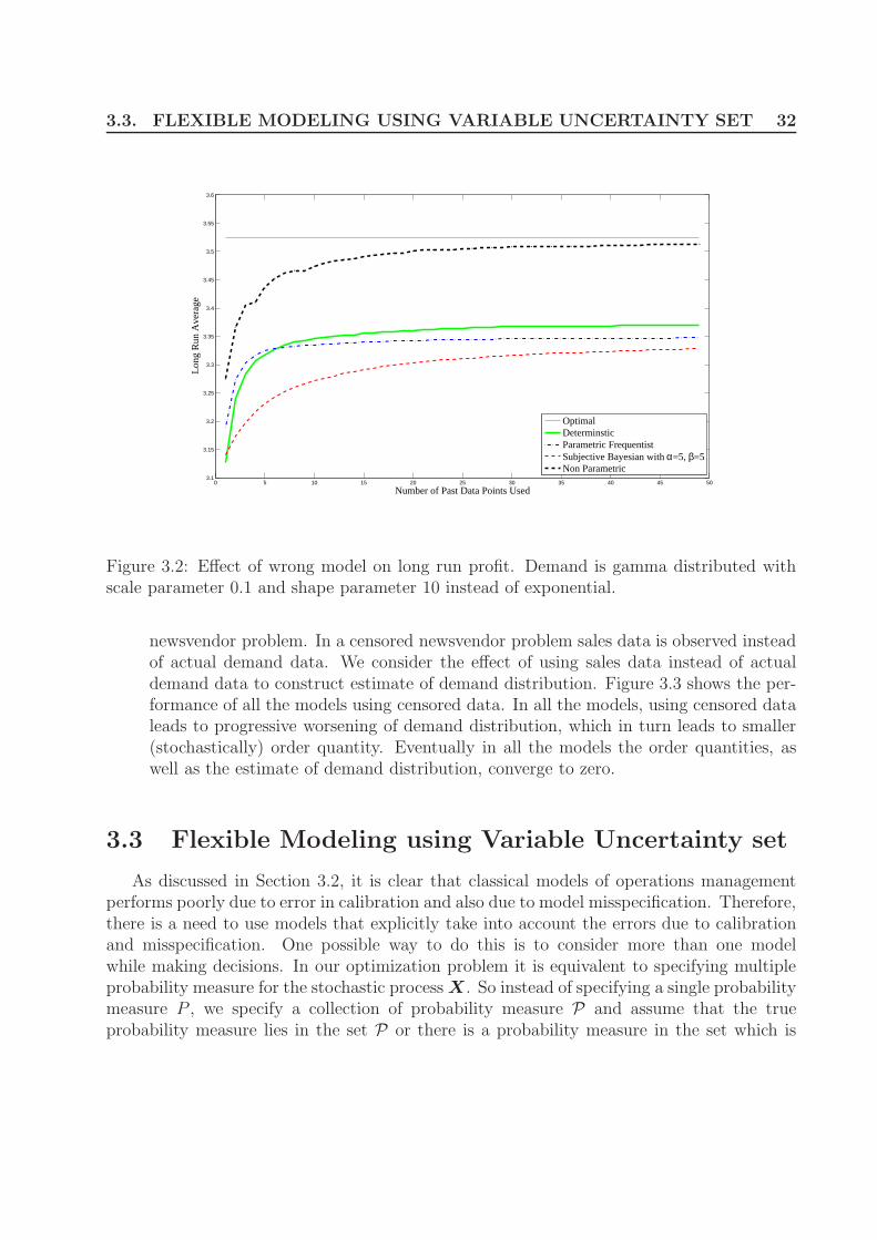
3.3. FLEXIBLE MODELING USING VARIABLE UNCERTAINTY SET 32
0 5 10 15 20 25 30 35 40 45 503.1
3.15
3.2
3.25
3.3
3.35
3.4
3.45
3.5
3.55
3.6
Number of Past Data Points Used
Long
Run
Ave
rage
OptimalDeterminsticParametric FrequentistSubjective Bayesian with α=5, β=5Non Parametric
Figure 3.2: Effect of wrong model on long run profit. Demand is gamma distributed withscale parameter 0.1 and shape parameter 10 instead of exponential.
newsvendor problem. In a censored newsvendor problem sales data is observed insteadof actual demand data. We consider the effect of using sales data instead of actualdemand data to construct estimate of demand distribution. Figure 3.3 shows the per-formance of all the models using censored data. In all the models, using censored dataleads to progressive worsening of demand distribution, which in turn leads to smaller(stochastically) order quantity. Eventually in all the models the order quantities, aswell as the estimate of demand distribution, converge to zero.
3.3 Flexible Modeling using Variable Uncertainty set
As discussed in Section 3.2, it is clear that classical models of operations managementperforms poorly due to error in calibration and also due to model misspecification. Therefore,there is a need to use models that explicitly take into account the errors due to calibrationand misspecification. One possible way to do this is to consider more than one modelwhile making decisions. In our optimization problem it is equivalent to specifying multipleprobability measure for the stochastic process X. So instead of specifying a single probabilitymeasure P , we specify a collection of probability measure P and assume that the trueprobability measure lies in the set P or there is a probability measure in the set which is

3.3. FLEXIBLE MODELING USING VARIABLE UNCERTAINTY SET 33
Figure 3.3: Spiral down effect observed using censored demands
3.3. FLEXIBLE MODELING USING VARIABLE UNCERTAINTY SET 34
very close (in some sense) to the true probability measure. The variable uncertainty set Pcan be defined in both parametric and non-parametric ways.
3.3.1 Deterministic Variable Uncertainty Set
The deterministic uncertainty set is a collection of degenerate probability measure, i.e.,
PD = PDω , ω ∈ Ω. (3.38)
This is essentially equivalent to defining a set of values that X can take. Let the set ofpossible values be X . Then one considers a collection of problems:
ψ(y,X), X ∈ X . (3.39)
In the newsvendor problem, where Dlkk is the forecast of the future, the deterministic
uncertainty set is given by:
DDk = D : Dlk
k − ak ≤ D ≤ Dlkk + bk (3.40)
In practice it is hard to come up with values of ak and bk unless there are natural limits orengineering application. A natural limit can be found by using population size, but usingthe population size is not expected to give a good solution as we shall see in the next section.
Another possible way to get ak’s and bk’s is to use confidence interval associated withDlk
k assuming lk is sufficiently large so that distribution of Dlkk is close to normal. The values
of ak and bk then would be:
ak = Dlkk − zα/2
Slkk
lk, bk = Dlk
k + zα/2Slk
k
lk, (3.41)
for appropriate value of α, 0 < α < 1. Slkk is the standard deviation of last lk entries.
3.3.2 Parametric Variable Uncertainty Set
A possible way to consider the error in calibration of a parametric model is to considera family of probability measures based on different values of parameter. In a parametricfrequentist setting the collection of measures we consider could be
PPF = P PFθ , θ ∈ Θ, (3.42)
for some set Θ of parameter values.It is common in robust optimization to specify set Θ using a confidence set for θ. Let
0 < α < 1 and t (I0) be an estimator of θ given initial information I0. The uncertainty set
3.3. FLEXIBLE MODELING USING VARIABLE UNCERTAINTY SET 35
Θ is chosen so that
P (t (I0) ∈ Θ) = 1 − α. (3.43)
One problem here is how to choose an appropriate value of α, as the solution is dependenton α. A robust solution is desirable if it is not too sensitive to the choice of α.
For the newsvendor problem if the past lk periods data is assumed to be i.i.d. exponentialthen it can be shown that:
2lkθDlk
k =d χ22lk, (3.44)
where χ22lk
is a chi-square random variable with 2lk degrees of freedom. From (3.43) and (3.44)it is immediate that
P
(
2lkDlkk
χ22lk , α
2
≤ θ ≤2lkD
lkk
χ22lk,1−α
2
)
= 1 − α, (3.45)
wherePχ2
2lk,β ≤ χ22lk = β, β ≥ 0.
A (1 − α) 100 % confidence interval for θ is
(
2lkDlkk
χ22lk, α
2
,2lkD
lkk
χ22lk,1− α
2
)
which can be used as set
Θ.A Bayesian way to specify the variable uncertainty set is to consider hierarchical models.
If the parameters of prior distribution are not well specified then in true Bayesian sensewe should consider the parameters of prior distribution itself to be random and specify aprobability measure on parameters. We can consider multiple levels of hierarchy, though inpractice it is not advantageous to have more than two or three levels of hierarchy.
3.3.3 Nonparametric Variable Uncertainty Set
There are multiple ways to specify a non-parametric uncertainty set. One particular wayis to specify some properties about the distribution of the stochastic process and consider theclass of all probability measures that satisfy those properties. For example a non-parametricvariable uncertainty set can be a set of all probability measures such that the mean vectorand covariance matrix of the stochastic process are some particular values, i.e.,
P = P : EP [X] = µ,EP [(X − µ)(X − µ)′] = Q. (3.46)
A non-parametric variable uncertainty set can also be specified by choosing a ball of prob-ability measure centered around a nominal probability measure. All measures in the ballare within some ”distance“ from the nominal probability measure. Therefore, to completely

3.3. FLEXIBLE MODELING USING VARIABLE UNCERTAINTY SET 36
specify a non-parametric variable uncertainty set we need a nominal probability measure anda measure of distance between probability measures. One way to specify nominal probabil-ity measure is to choose it non-parametrically as in Section 3.1.2, although we can specifya parametric nominal probability measure while still choosing the variable uncertainty setnon-parametrically. If P is the nominal probability measure and d(P, P ) is a measure ofdistance between P and P , then a non-parametric variable uncertainty set is:
P = P : d(P, P ) ≤ α, (3.47)
for some parameter value α. Ideally we would like to choose α so that the true probabilitymeasure is in P. In practice it may be hard to choose such an α but we hope that oursolution is not too sensitive to α and a reasonable choice of α would give us a robust enoughsolution.
Some of the distance measures commonly used are listed below:
Kullback-Leibler(KL) Divergence or Relative Entropy
dKL(P, P ) =
∫
Ω
log
(
dP
dP
)
dP, (3.48)
where dP
dPis so called Radon-Nikodym derivative. Kullback-Leibler divergence is a popular
measure to specify variable uncertainty sets specifically in dynamic models. It has a usefulproperty that it is sum separable for product measures. It is convex in P and takes valuesin [0,∞]. However, it is not a metric (it is not symmetric in (P, P ) and does not satisfythe triangle inequality). Another caveat is if there exists a set A, however small, such thatP (A) > 0 but P (A) = 0, then dKL(P, P ) = ∞.
Total Variation Distance
Total variation distance is defined as:
dTV (P, P ) = sup|P (A) − P (A)| : A ∈ F (3.49)
Total variation distance defines a norm on the space of probability measures.

3.4. ROBUST OPTIMIZATION MODELS 37
Levy (Prokhorov) Metric
Levy metric, which is a special case of Levy-Prokhorov metric, between two probabilitydistributions F and F is defined as
dL(F, F ) = infh : F (x− h) − h ≤ F (x) ≤ F (x+ h) + h; h > 0; x ∈ R. (3.50)
3.4 Robust Optimization Models
Assuming that the true probability measure can be any one from the variable uncertaintyset, robust optimization methods use suitable objective functions to derive solutions whichare hoped to be robust enough to model misspecification and calibration error. Some ofthe most commonly used objective functions are max-min, max-min regret and max-mincompetitive ratio.
3.4.1 Max-min Objective
The max-min or worst case objective is the most commonly used robust objective inoperations management literature. The optimization problem is:
maxy∈Y
minP∈P
E [ψ(y,X)] . (3.51)
This approach finds the best solution assuming the true model is the worst one possible. Ifthe variable uncertainty set is large then the solution might be too conservative. On theother hand if the uncertainty set is too small then the solution may not be robust at all. Inpractice we want a solution that is not too sensitive to the variable uncertainty set; min-maxas a robust objective fails to achieve that as we shall see in the newsvendor problem context.
Max-min with Deterministic Uncertainty Set
If the demand in period k can take values in [ak, bk], then the robust optimization problemis:
maxy≥0
minak≤Dk≤bk
n∑
k=1
(sminDk, yk − cyk) . (3.52)
Since the inner minimization is monotone in Dk, the optimization problem (3.52) can bewritten as:
maxy≥0
n∑
k=1
(smina, yk − cyk) , (3.53)

3.4. ROBUST OPTIMIZATION MODELS 38
0 5 10 15 20 25 30 35 400.4
0.45
0.5
0.55
0.6
0.65
0.7
0.75
0.8
0.85
0.9
Number of Past Data Points Used
Long
Run
Ave
rage
Max−Min DeterministicNominal Deterministic
Figure 3.4: Performance of Max-min robust optimization objective with deterministic un-certainty set.
with optimum solution
yR:Dk = ak, k = 1, 2, . . . , m. (3.54)
To implement the solution we need values for ak’s. A natural boundary is ak = 0 butthis would give a profit of 0, which is clearly a pessimistic solution.
Instead if we use the value of ak as defined in (3.41), the profit ψR:D is:
ψR:D =
n∑
k=1
smin
[
Dlkk − zα/2S
lkk
]+
, Dk
− c[
Dlkk − zα/2S
lkk
]+
. (3.55)
As we see from Figure 3.4, the performance of the deterministic max-min optimizationis even worse than deterministic optimization for 90% confidence interval estimates for α.We can, of course, improve the performance by choosing different values of confidence level.However, first it is difficult to say which value of confidence level is good a priori. In addition,as we see from Figure 3.5, the performance of the max-min deterministic robust optimizationcan be quite sensitive to the choice of α.

3.4. ROBUST OPTIMIZATION MODELS 39
0 0.05 0.1 0.15 0.2 0.25 0.3 0.35 0.4 0.45 0.50.5
0.55
0.6
0.65
0.7
0.75
0.8
0.85
α
Long
Run
Ave
rage
Pro
fit
Figure 3.5: Sesitivity of Max-min robust optimization (with deterministic uncertainty set)objective with respect to α .
Max-min with Parametric Uncertainty Set
Suppose the variable parametric uncertainty set in period k is ak ≤ θ ≤ bk. The robustoptimization problem in period k is:
maxyk≥0
minak≤θ≤bk
sθ(
1 − exp(
−yk
θ
))
− cyk (3.56)
As before the inner minimization is monotone in θ, and so it is immediate that
yR:PFk = ak log
(s
c
)
, k = 1, 2, . . . , m. (3.57)
To implement the solution, we can use confidence interval for θ as defined in (3.45). Therobust profit ψR:PF is:
ψR:PF =
n∑
k=1
smin
2lkDlkk
χ2lk,α/2
log(s
c
)
, Dk
− c2lkD
lkk
χ2lk ,α/2
. (3.58)
Figure 3.6 shows the performance of max-min robust parametric solution and classicalparametric solution for an uncertainty set corresponding to 90% confidence level. The per-

3.4. ROBUST OPTIMIZATION MODELS 40
0 5 10 15 20 25 30 35 40 45 50
0.65
0.7
0.75
0.8
0.85
0.9
0.95
1
Number of Past Data Points Used
Long
Run
Ave
rage
Nominal ParametricMax−Min Parametric
Figure 3.6: Performance of Max-min robust optimization with parametric uncertainty set
formance of robust solution is worse than classical point estimate based parametric solutionirrespective of the number of past data points used.
Max-min with Nonparametric Variable Uncertainty Set
The non-parametric uncertainty set for demand Dk in period k is the set of all probabilitydistribution with mean µk and variance σ2
k. It can be shown that maximizing the newsvendorprofit is equivalent to minimizing
yk +s
cEP [Dk − yk] . (3.59)
An upper bound on EP [Dk − yk], as proved in [GM94] is:
EP [Dk − yk] ≤(σ2
k + (yk − µk)2)
1/2− (yk − µk)
2. (3.60)
The order quantity yNPk that minimizes the upper bound is:
yR:NPk = µk +
σk
2
(
(
s− c
c
)1/2
−
(
c
s− c
)1/2)
. (3.61)
3.4. ROBUST OPTIMIZATION MODELS 41
To actually implement this policy we need estimates of µk and σk. Let the estimates basedon past lk periods of data be:
µlkk =
1
lk
k−1∑
i=k−lk
Dk, and (3.62)
σlkk =
1
lk − 1
k−1∑
i=k−lk
(Dk − µlkk )1/2. (3.63)
The implemented policy is:
yR:NPk = µlk
k +σlk
k
2
(
(
s− c
c
)1/2
−
(
c
s− c
)1/2)
. (3.64)
The profit ψR:NP corresponding to policy yR:NPk is:
ψR:NP =n∑
k=1
(
smin
yR:NPk , Dk.
− cyR:NPk
)
. (3.65)
Figure 3.7 compare the performance of max-min robust non-parametric solution and classicalnon-parametric solution for an uncertainty set corresponding to 90% confidence level. Thereis not much difference between the performance of robust solution and that of a classicalnon-parametric solution.
3.4.2 Min-max Regret
Max-min objectives choose the worst model out of all permissible ones. If the modelhappens to be best one possible then the performance of a robust max-min solution isvery bad. There is an opportunity cost if the true model is best one and the solutionis too conservative. Min-max regret find a solution by minimizing this opportunity cost.Mathematically, a min-max regret objective is:
miny∈Y
maxP∈P
EP [ψ(y∗(P ),X) − ψ(y,X)] , (3.66)
where y∗(P ) is the optimal solution under the probability measure P . The notion of regretis more appealing than worst-case optimization as it sought to achieve a middle groundbetween optimistic and pessimistic scenarios.

3.4. ROBUST OPTIMIZATION MODELS 42
0 5 10 15 20 25 30 35 400.75
0.8
0.85
0.9
0.95
1
Number of Past Data Points Used
Long
Run
Ave
rage
Max−Min Non ParametricNominal Non Parametric
Figure 3.7: Performance of Max-min robust optimization with non-parametric uncertaintyset
Min-Max Regret with Deterministic Variable Uncertainty Set
If the demand in period k is known to be deterministically D then the optimal profit is(s− c)D. So the regret objective in period k, if the deterministic uncertainty set is [ak, bk],is:
minyk
maxak≤Dk≤bk
((s− c)Dk − sminyk, Dk − cyk) . (3.67)
For a given yk the objective is convex in Dk. Hence, the objective in (3.67) can be writtenas:
minyk
max(s− c)ak − sak − cyk, (s− c)bk − syk − cyk. (3.68)
The solution yk would be such that:
(s− c)ak − sak − cyk = (s− c)bk − syk − cyk. (3.69)
Hence
yk = ak + (bk − ak)s− c
s. (3.70)
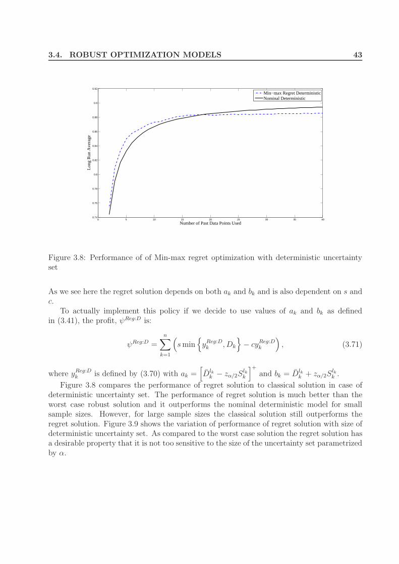
3.4. ROBUST OPTIMIZATION MODELS 43
0 5 10 15 20 25 30 35 400.74
0.76
0.78
0.8
0.82
0.84
0.86
0.88
0.9
0.92
Number of Past Data Points Used
Long
Run
Ave
rage
Min−max Regret DeterministicNominal Deterministic
Figure 3.8: Performance of of Min-max regret optimization with deterministic uncertaintyset
As we see here the regret solution depends on both ak and bk and is also dependent on s andc.
To actually implement this policy if we decide to use values of ak and bk as definedin (3.41), the profit, ψReg:D is:
ψReg:D =
n∑
k=1
(
smin
yReg:Dk , Dk
− cyReg:Dk
)
, (3.71)
where yReg:Dk is defined by (3.70) with ak =
[
Dlkk − zα/2S
lkk
]+
and bk = Dlkk + zα/2S
lkk .
Figure 3.8 compares the performance of regret solution to classical solution in case ofdeterministic uncertainty set. The performance of regret solution is much better than theworst case robust solution and it outperforms the nominal deterministic model for smallsample sizes. However, for large sample sizes the classical solution still outperforms theregret solution. Figure 3.9 shows the variation of performance of regret solution with size ofdeterministic uncertainty set. As compared to the worst case solution the regret solution hasa desirable property that it is not too sensitive to the size of the uncertainty set parametrizedby α.

3.4. ROBUST OPTIMIZATION MODELS 44
0 0.05 0.1 0.15 0.2 0.25 0.3 0.35 0.4 0.45 0.50.5
0.55
0.6
0.65
0.7
0.75
0.8
0.85
0.9
0.95
α
Long
Run
Ave
rage
Pro
fit
Figure 3.9: Sensitivity of Min-max regret optimization (with deterministic uncertainty set)with α.
Min-Max Regret with Parametric Variable Uncertainty Set
With parameter of exponential lying in [ak, bk], the min-max regret problem in period kis
minyk
maxak≤θ≤bk
Eθ
[
(s− c)θ − cθ log(s
c
)
− sminyk, Dk + cyk
]
(3.72)
which can be written after taking expectation as
minyk
maxak≤θ≤bk
[
θ
(
s exp
(
−yk
θ
)
− cθ(1 + log(s/c))
)
+ cyk
]
(3.73)
It can be shown that the optimal yk can be found by equating regrets at θ = ak and θ = bk.The optimum yk is the solution of the following equation:
(bk − ak)c
s
(
1 + log(s
c
))
= bk exp(−yk/bk) − ak exp(−yk/ak). (3.74)

3.4. ROBUST OPTIMIZATION MODELS 45
0 5 10 15 20 25 30 35 400.1
0.2
0.3
0.4
0.5
0.6
0.7
0.8
0.9
1
Number of Past Data Points Used
Long
Run
Ave
rage
Min−max Regret ParametricNominal Parametric
Figure 3.10: Performance of of Min-max regret optimization with parametric uncertainty set
We can use confidence interval for θ as defined in (3.45) for ak and bk. The profit functionψReg:PF is
ψReg:PF =n∑
k=1
(
smin
yReg:PFk , Dk
− cyReg:PFk
)
, (3.75)
with yReg:PFk is solution of (3.74) with ak =
2lkDlkk
χ2lk,α/2and bk =
2lkDlkk
χ2lk,1−α/2.
Figure 3.10 compares the performance of regret solution with classical parametric solutionfor 90% confidence parametric uncertainty set. Even though the performance of regretsolution is better than the worst case solution, it is still worse than the classical parametricsolution for all sample sizes.
Max-min Regret with Nonparametric Variable Uncertainty Set
We consider the the non-parametric uncertainty set for demand Dk in period k is theset of all probability distribution with mean µk. It can be shown (See [PR08]) that orderquantity that minimize the maximum regret is:
yReg:NPk =
µk
(
1 − cs
)
if 12≤ c
sµk
4 cs
if 12> c
s(3.76)
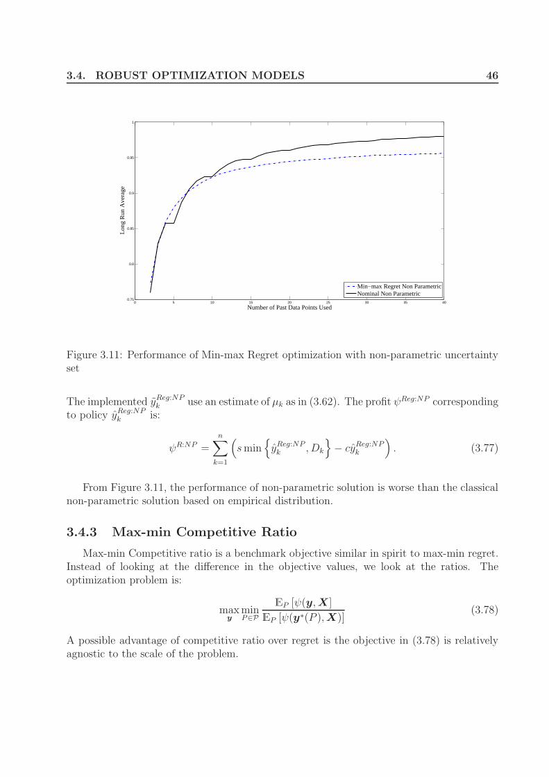
3.4. ROBUST OPTIMIZATION MODELS 46
0 5 10 15 20 25 30 35 400.75
0.8
0.85
0.9
0.95
1
Number of Past Data Points Used
Long
Run
Ave
rage
Min−max Regret Non ParametricNominal Non Parametric
Figure 3.11: Performance of Min-max Regret optimization with non-parametric uncertaintyset
The implemented yReg:NPk use an estimate of µk as in (3.62). The profit ψReg:NP corresponding
to policy yReg:NPk is:
ψR:NP =n∑
k=1
(
smin
yReg:NPk , Dk
− cyReg:NPk
)
. (3.77)
From Figure 3.11, the performance of non-parametric solution is worse than the classicalnon-parametric solution based on empirical distribution.
3.4.3 Max-min Competitive Ratio
Max-min Competitive ratio is a benchmark objective similar in spirit to max-min regret.Instead of looking at the difference in the objective values, we look at the ratios. Theoptimization problem is:
maxy
minP∈P
EP [ψ(y,X]
EP [ψ(y∗(P ),X)](3.78)
A possible advantage of competitive ratio over regret is the objective in (3.78) is relativelyagnostic to the scale of the problem.
3.4. ROBUST OPTIMIZATION MODELS 47
Max-min Competitive Ratio with Deterministic Variable Uncertainty Set
The competitive ratio optimization problem in period k (assuming ak > 0) is
maxyk
minak≤Dk≤bk
sminyk, Dk − cyk
(s− c)Dk. (3.79)
The optimal yk can be found by solving the following:
sak − cyk
ak=syk − cyk
bk, (3.80)
from which we obtain
yk =sakbk
c(bk − ak) + sak. (3.81)
If we use values of ak and bk as defined in (3.41), the profit, ψC:D is:
ψC:D =n∑
k=1
(
smin
yC:Dk , Dk
− cyC:Dk
)
, (3.82)
where yC:Dk is defined by (3.81) with ak = max
Dlkk − zα/2S
lkk , ǫ
and bk = Dlkk + zα/2S
lkk .
ǫ > 0 is small parameter added to make ak > 0.Figure 3.12 compares the performance of the solution derived from competitive ratio
objective (uncertainty set constructed using 90% confidence level) to the performance ofthe classical deterministic solution. The competitive ratio solution outperforms the classicaldeterministic solution for nearly all sample sizes. Hence, as a robust objective it works muchbetter than regret and worst case optimization objectives for the newsvendor problem. Inaddition, as we see from Figure 3.13 the performance of the competitive ratio solution is notmuch sensitive to the size of uncertainty set.
Max-min Competitive Ratio with Parametric Variable Uncertainty Set
As before the max-min competitive ratio problem in period k with variable parametricuncertainty is
maxyk
minak≤θ≤bk
sθ(
1 − exp(
−yk
θ
))
− cyk
θ(
(s− c) − log(
sc
)) . (3.83)
For a given yk the above objective has maximum at θ = yk
ln(s/c), decreasing on either side of
it. In addition, the function is concave in yk. It can be proved that the optimal policy yk is

3.4. ROBUST OPTIMIZATION MODELS 48
0 5 10 15 20 25 30 35 400.55
0.6
0.65
0.7
0.75
0.8
0.85
0.9
0.95
Number of Past Data Points Used
Long
Run
Ave
rage
Max−min Competitive Ratio DeterministicNominal Deterministic
Figure 3.12: Performance of Max-min competitive ratio optimization with deterministicuncertainty set
0 0.05 0.1 0.15 0.2 0.25 0.3 0.35 0.4 0.45 0.50.5
0.55
0.6
0.65
0.7
0.75
0.8
0.85
0.9
0.95
α
Long
Run
Ave
rage
Pro
fit
Figure 3.13: Sensitivity of Max-min competitive ratio optimization (with deterministic un-certainty set) with α.

3.4. ROBUST OPTIMIZATION MODELS 49
0 5 10 15 20 25 30 35 400.75
0.8
0.85
0.9
0.95
1
Number of Past Data Points Used
Long
Run
Ave
rage
Max−min Competitive Ratio ParametricNominal Parametric
Figure 3.14: Performance of Max-min competitive ratio optimization with parametric un-certainty set
given by solution of the following:
sak
(
1 − exp(
− yk
ak
))
− cyk
ak
=sbk
(
1 − exp(
−yk
bk
))
− cyk
bk. (3.84)
We can implement the policy by solving for yk with ak and bk given by (3.45). If the solutionis yC:PF
k , the profit function ψC:PF is:
ψC:PF =
n∑
k=1
(
smin
yC:PFk , Dk
− cyC:PFk
)
. (3.85)
Figure 3.14 compares the performance of the competitive ratio solution with parametricuncertainty set to the solution of the classical parametric solution. The performance ofcompetitive ratio solution is close to the classical parametric solution but is still uniformlyworse than the classical solution for all sample sizes. This is in contrast to the competitiveratio with deterministic uncertainty set, where the robust solution outperforms the classicaldeterministic solution.
The comparison of various robust optimization models when uncertainty set is calculatedfrom past data shows that most of the time performance of robust models is even worse

3.5. LEARNING 50
than their non-robust counterparts. Next we discuss some objective learning approachesthat integrate optimization and learning.
3.5 Learning
3.5.1 Reinforcement Learning
Reinforcement learning as a learning paradigm falls between supervised and unsupervisedlearning. Learning is done through trial and error by providing reinforcement or reward inresponse to an action. The method is particularly suitable for learning in dynamic environ-ment without making too many assumptions about the underlying process or environment.The basic premise of reinforcement learning is to learn the best action in a given “state”by exploiting the current best action and also by randomly exploring other actions. The“state” can be understood to be a finite dimensional vector which is an input to the system.An example of a state is the initial inventory at the start of a period in inventory controlproblem. The system tries to learn the “value” of the state, which is the reward obtainedby implementing an optimal policy through a reinforcement learning algorithm. Some ofthe popular reinforcement learning algorithms are TD(λ) [Sut88], Q learning [Wat89], andDyna [Sut90]. For a survey of reinforcement learning algorithms see [SB98] and [KLM96].
The newsvendor problem, which is an example of sequential decision making, can be for-mulated as a multiple arm bandit problem, which is a special case of reinforcement learningwith single state but multiple actions. Although the action (order quantity) space is con-tinuously valued, we can get a good approximation by discretization the action space intofinitely many values then applying an algorithm such as UCB1 [ACBF02] for multi-armedbandit on the discretized problem. A better approach would be to apply continuum armbandit algorithm [Kle04], as the newsvendor profit function is Lipschitz continuous in orderquantity. An advantage of multi-arm bandit approach is that we can theoretically boundthe cumulative regret of the algorithm. On the other hand the small sample performance ofmulti-arm bandit algorithm does not utilize much structural and distributional informationabout the problem in hand.
3.5.2 Objective Bayesian
The main criticism of subjective Bayesian methods is subjectivity in choosing the priorfor the parameters of distribution of stochastic process. It is often difficult to find an“expert” who can provide a good subjective prior. As we have seen from Figure 3.1 thesolution does depend heavily on the choice of prior. A possible alternative is to use non-informative/objective priors. A non-informative prior can informally be defined as the onewhich favors no particular value of parameter over others. One particular way to define
3.5. LEARNING 51
non-informative is to use Jefferys prior [Jef46], which is to use
fΘ(θ) ∝ (I(θ))1/2 (3.86)
as non-informative prior, where I(θ) is the expected Fisher information. Under some com-monly satisfied assumptions [Ber85] I(θ) is given by
I(θ) = −Eθ∂2 logPθ
∂θ2. (3.87)
For an exponential distribution with mean θ, the expected Fisher information I(θ) is(
1θ
)2,
and a non-informative prior is:
fΘ(θ) =1
θ, θ > 0.. (3.88)
Note that the prior (3.88) is not a proper probability density over (0,∞) as∫
(0,∞)1θdθ = ∞.
However, we may still use fΘ(θ) as a probability density in Bayes’ rule if the posterior is aproper probability density.
For the newsvendor problem, if in period k we use past lk periods of data to make thedecision then the posterior distribution using prior (3.88) is
fkΘ(θ) =
lkDlkk
(lk − 1)!θlk+1exp
(
−lkD
lkk
θ
)
. (3.89)
Hence the marginal distribution of Dk is
fDk(x) =
∫
Θ
(
lkDlkk
)lk
(lk − 1)!θlk+2exp
(
−lkD
lkk + x
θ
)
dθ. (3.90)
which is equal to
fDk(x) =
lk
(
lkDlkk
)lk
(
lkDlkk + x
)lk+1. (3.91)
Hence
FDk(x) =
(
lkDlkk
lkDlkk + x
)lk
. (3.92)
3.5. LEARNING 52
Therefore, the optimal order quantity yOB = F−1Dk
(c/s) is:
yOB = Dlkk lk(
(s/c)1/lk − 1)
. (3.93)
Objective Bayesian learning provides an attractive way to make decisions in the presenceof model uncertainty. Later in Chapter 4 we will see this is (in a way) the best we can do.
However, objective Bayesian can also be criticized similarly to subjective Bayesian asthere is no unique way of defining a non-informative prior. For example, for Normal dis-tribution with mean µ and variance σ2, Jefferys prior is 1
σ2 . Another commonly used non-informative prior is 1
σ. It is not clear which prior to be used for a particular problem. In
addition, similar to subjective Bayesian method the prior should be chosen independent ofobjective function.
3.5.3 Classical Decision Theory
In classical (non-Bayesian) decision theory a non-randomized decision rule y is a mappingfrom the available information to the policy space. So the decision at time k, yk is directlya function of the information set Ik. We denote the dependency of y on information setby y(I). A classical decision theorists seeks to evaluate the “loss” for every value of theparameter of the underlying stochastic process. The loss is measured by using a risk function.In the setup where profit is maximized we can use the negative of the profit function as risk.Equivalently we can focus on
maxy
Eθ [ψ(y(I),X(θ)] . (3.94)
As the frequentist risk or profit function is a function of θ, it is not clear what maximiz-ing (3.94) actually means. A partial ordering of decision rules can be formed by utilizing thefollowing notion:
Definition 7. A decision rule y(I) is better than y′(I) if
Eθ [ψ(y(I),X(θ)] ≥ Eθ [ψ(y′(I),X(θ)] ∀ θ (3.95)
with strict inequality for at least one θ.
Definition 8. A decision rule is admissible if there exists no better decision rule as definedin Definition 7.
Naturally it makes sense to search only for decision rules which are admissible. However,the class of admissible decision rules is very large. If we fix a particular value of θ, say θ0and let y be the optimal decision for θ0 regardless of past data values or information, thenit is likely that y is admissible. However, such a decision rule is likely to perform quite badfor other values of θ. On the other hand we can define the concept of an optimal decisionrule as follows:
3.6. DISCUSSION 53
Definition 9. A policy y is optimal, if
Eθ [ψ(y(I),X(θ))] ≥ Eθ[[ψ(y′(I),X(θ))] , ∀ θ, (3.96)
for all possible y′.
Such a concept, though attractive, is quite restrictive. Indeed the class of problems whereone can find a decision rule in the sense of (3.96) is quite small. Therefore, there is a need todefine alternative concepts of choosing decision rules. In classical decision theory, there arethree major methods [Ber85] of choosing decision rules. First is Bayes Risk Principle wherethe risk or profit function is integrated over θ using a prior on θ. The method is not toodifferent from subjective Bayesian principle discussed in Section 3.1.2, and can be criticizedsimilarly for subjectivity in choosing the prior distribution. Second is Invariance Principle
which informally states that a decision rule should not depend on the unit of measurementused or any other such arbitrary structure. There is a direct correspondence of such ruleswith method of using non-informative priors and hence we will not discuss it here. Thirdis the Max-min Principle. The aim is to choose a decision rule that maximize the profitassuming the worst possible parameter of stochastic process. Such a concept is similar torobust optimization, the difference being the policy is a function of past data/information.
3.6 Discussion
In this chapter, we have studied the effect of model uncertainty on various classical mod-eling approaches. We studied many popular robust optimization approaches and comparedthe performance to their non-robust counterparts. If the performance is compared on thebasis of next period expected profit, then most of the time performance of robust solutionsis even worse than the classical non-robust solutions. In Chapter 4, we introduce generalizedoperational statistics approach, which is a parametric approach that guarantees a bettersolution than a classical solution over a set of parameter.
In Section 3.2.2, we also discussed the effect of using wrong model class and wrongstatistical assumption. When confidence in a particular model class is low it is desirable touse a non-parametric method such as reinforcement learning. In Chapter 6 we introduce anew non-parametric learning method, which utilizes the structural information embedded ina problem to improve small sample performance.

54
Chapter 4
Operational Statistics
In Chapter 3, we discussed different approaches for modeling uncertainty with learning.In almost all these approaches the learning and optimizations tasks are separated. Firstthe parameters of the model are statistically estimated, and then optimization is done onthe resulting model assuming that the estimated parameters are true ones. Operationalstatistics (OS) is an integrated learning and optimization approach to model uncertainty.The OS approach was first introduced in [LS05] and further explored in [CSS08]. Thepapers [LS05] and [CSS08] have successfully applied operational statistics to the parametricsetting where the unknown parameters are either scale or shift parameters. In this chapterwe generalize the operational statistics approach and in Chapter 5, we apply the approachto mean variance portfolio optimization problem. Below we present a brief introduction tothe operational statistics approach as applied to the newsvendor problem [LS05]. We thenpresent a generalization of this apporach.
4.1 Operational Statistics
Consider the newsvendor problem as defined in Chapter 3. The expected profit when theorder quantities and the realized demands in first n periods are y1, . . . , yn and D1, . . . , Dn
respectively is:
φ(y) =n∑
k=1
E [smin yk, Dk − cyk] . (4.1)
If we know the distribution of the demand then it is well known that the optimal orderquantity in every period is F 1
(
cs
)
where F is the distribution function of the demand. Nowconsider the case when the demand is exponentially distributed with unknown parameterθ. If parameter θ is known then the optimal order quantity is θ ln
(
cs
)
. When θ is unknownone particular method that is frequently used in the literature is to replace θ by its pointestimate at every time instant. When θ is a scale parameter a point estimate of θ for period

4.1. OPERATIONAL STATISTICS 55
k using past lk periods of demand data is:
θk = Dlkk =
1
lk
k−1∑
i=k−lk
Di. (4.2)
Hence the order quantity yk, using the estimate θk is:
yk = Dlkk ln
(s
c
)
. (4.3)
If we use the order quantity yk, then using equation (4.1), the a priori expected profit φsm
as a function of θ is:
φsm(θ) = Eψsm(D) =
n∑
k=1
E
[
smin
Dlkk ln(
(s
c
)
, Dk
− cDlkk ln
(s
c
)]
=
n∑
k=1
cθ
[
s
c−s
c
(
lklk + ln(s/c)
)lk
− ln(c
s
)
]
.
(4.4)
In operational statistics an order quantity, rather than the parameters of the distribution, isdirectly estimated from the data. In this sense, the approach is similar to the policy gradientand direct reinforcement methods mentioned in the reinforcement learning literature (seeBaxter and Bartlett [BB01] and Moody and Saffell [MS01]. However, in operational statisticsthe order quantity is estimated in such a way that the a priori expected profit is maximized,rather than doing trial and error and fine-tuning the parameters using gradients in policyspace. The latter approach requires extensive amount of data before it performs well andis unsuitable for most of the problems where past data is not readily available. Even if thedata is available, it is not necessary that the statistical assumptions (such as i.i.d. demands)are valid over a long run of time.
The idea of operational statistics is as follows: we consider order quantities to be statisticsof the data D1, D2, . . . , Dn within some acceptable class parametrized by some optimiza-tion variables, say z. This statistics is called operational statistics as the statistics is drivenby the operational problem, not by the estimation problem. One then finds an optimaloperational statistics within the class by maximizing the expected a priori profit over thevariables z. Specifically for the problem in hand, where the demand is exponential withunknown scale parameter θ, the order quantity is chosen to be of the form
yk(zk) = zkDlkk , z ≥ 0. (4.5)

4.1. OPERATIONAL STATISTICS 56
The a priori expected profit φos(θ) using the estimate yk is
φos(θ) =n∑
k=1
E
[
smin
zkDlkk , Dk
− czkDlkk
]
=n∑
k=1
cθ
[
s
c−s
c
(
lklk + zk)
)lk
− zk
]
.
(4.6)Optimizing over zk we get
z∗k = lk
(
(s
c
)1/(lk+1)
− 1
)
. (4.7)
The operational statistics order quantity is
yk = lk
(
(s
c
)1/(lk+1)
− 1
)
Dlkk . (4.8)
Realized profit ψOS using operational statistics is
ψOS(D) =n∑
k=1
[
smin
lk
(
(s
c
)1/(lk+1)
− 1
)
Dlkk , Dk
− clk
(
(s
c
)1/(lk+1)
− 1
)
Dlkk
]
.
(4.9)Consider the situation where the underlying process Dk is locally stationary. At every
time instant only last m periods of data can be considered approximately i.i.d,. and thereforewe use lk = m for every k. Long run average profit of the operational statistics strategywould be
limn→∞
ψOS(D)
n= E
[
smin
m
(
(s
c
)1/(m+1)
− 1
)
Dmk , Dk
− cm
(
(s
c
)1/(m+1)
− 1
)
Dmk
]
= θ
[(
s− s(c
s
)m/(m+1))
− cm
(
(s
c
)1/(m+1)
− 1
)]
.
(4.10)
Compare (4.10) to the long run average cost of using a trailing m period sample meanstrategy
limn→∞
ψOS(D)
n= θ
[
s− s
(
m
m+ ln(s/c)
)m
− c ln(c
s
)
]
. (4.11)
Since the operational statistics order quantity (4.8) maximizes the a priori expected profitover all order quantities of the form zDlk
k , z ≥ 0, the expected (or long run average) profitobtained from the operational statistics approach (4.10) is higher than the profit obtainedfrom the sample mean based approach (4.11) for all choices of m. On the other hand, as seenin Chapter 3, none of the robust optimization approaches guarantees a uniformly better(ina priori expected profit sense) solution than a simple sample mean based approach. As wesee from a sample simulation shown in Figure (4.1) for parameters s = 2, c = 1 and θ = 1,the improvement can be quite significant for small values of m.

4.1. OPERATIONAL STATISTICS 57
0 2 4 6 8 10 12 14 16 18 200
5
10
15
20
25
30
35
40
Number of Past Data Points Used
Per
cent
age
Long
Run
Ave
rage
Incr
ease
in P
rofit
Figure 4.1: Operational statistics policy is uniformly better than the sample mean basedpolicy for newsvendor problem
Note that in equation (4.7), the optimal zk is independent of θ. This is because theunknown parameter θ acts as a scaling parameter in the profit function (4.6). It is shownin [LS05], when the unknown parameter is a scale parameter (e.g. mean in exponential dis-tribution or normal distribution with unknown mean) and the class of operational statisticsis linear in sample mean, the optimal operational statistics is independent of the scaling pa-rameter for newsvendor problem. The paper [CSS08] extended the result of [LS05] to a classof homogeneous order one function and two parameter families (scale and shift). They alsoshowed a connection of operational statistics to objective Bayesian decision theory. However,the class of problems where an optimal operational statistics is independent of the underlyingunknown parameter is very limited or difficult to find.
4.1.1 Generalized Operational Statistics
A defining feature of operational statistics, as mentioned above, is that it guarantees abetter solution than the classical estimation based policy. However, it is either very hardor impossible to find a statistics such that the corresponding profit is uniformly better thanthe profit of a classical estimation based policy over the full range of parameter. Supposein addition the decision maker knows for sure that the unknown parameter lies in a knownuncertainty set Θ. Our objective is to improve the performance of classical policy over therange Θ. In other words, we want to ensure that the performance of operational statistics
4.1. OPERATIONAL STATISTICS 58
policy is better than the classical estimation based policy over the set Θ. A generalizedversion of operational statistics is implemented as follows:
Suppose we are interested in maximizing the function Eθψ(y,D) over y. If the value ofθ is known an optimal policy is y(θ). In the absence of true knowledge about θ, a classicalestimation based policy is y(θ), where θ is an estimate of θ. In addition, the decision makerknows or strongly believes that the parameter θ lies in a set Θ. We choose a set of functionsF , such that F defines a class of operational statistics. Each function f ∈ F defines amapping from past data D to a decision y. The function class F is such that the classicalestimation based decision rule y(θ) belongs to F . In addition we choose a representativeparameter θ and solve the following optimization problem:
Operational Statistics Formulation 1
maxf∈F
Eθψ(f(D),D)
such that
Eθψ(f(D),D) ≥ Eθψ(y(θ),D) ∀θ ∈ Θ
(4.12)
The representative parameter ˜theta is subjective knowledge of the decision maker inde-pendent from the data. Thus, the decision maker wants to utilize her subjective information,but because she is not sure about her subjective knowledge, wants a solution that is guaran-teed to perform better than the classical solution over the acceptable range of parameters.As y(θ) belongs to F , y(θ) is a feasible solution of (4.12) and hence the optimization prob-lem (4.12) is feasible. Also even though the choice of θ is subjective, the constraints inthe optimization problem ensure that the operational statistics solution is better than theclassical solution over the set Θ, and hence ensures robustness of the solution with respectto the parameter θ. Instead of using a single parameter θ, we can also use a subjective prioron θ. Let Pθ be the choice of the prior. Following is the version of operational statisticsproblem with subjective prior:
Operational Statistics Formulation 2
maxf∈F
∫
Θ
Eθψ(f(D),D)Pθ
such that
Eθψ(f(D),D) ≥ Eθψ(y(θ),D) ∀θ ∈ Θ
(4.13)
As the operational statistics solution is guaranteed to perform better than classical solution,

4.1. OPERATIONAL STATISTICS 59
and a classical solution converges to the true solution when θ → ∞, the operational statisticssolution would also converge to the true solution. The uncertainty set Θ, on the other hand,is held fixed and is not updated in response to the past data. It is also possible to usesome other benchmark instead of classical estimation policy in the operational statisticsformulation.

60
Chapter 5
Application of Operational Statisticsto Portfolio Optimization
In this chapter, we consider an important application of operational statistics approachdefined in Chapter 4 in mean variance portfolio optimization problem.
5.1 Mean-Variance Portfolio Optimization
We consider the problem of finding a mean variance optimal portfolio. The investor’sproblem is to find an optimal allocation to m-risky assets and a risk-free asset. Let µ be thevector of mean excess returns (return - risk free rate) and Σ be the covariance matrix. Weassume that the portfolio returns are normally distributed. The investor wishes to maximizethe following mean variance utility function:
maxπ
π′µ −1
2γπΣπ, (5.1)
where π is the vector of portfolio weights and γ is the risk aversion factor. The fraction 1−π′e
is invested in the risk free asset. Note that we do not have any short selling constraints.The problem can be solved analytically if we have exact knowledge of parameters µ and
Σ. In fact, the solution is π = 1γΣ−1µ. In reality, obtaining an accurate estimate of µ is
quite difficult. For example, if the return of a stock is generated from a normal distributionwith mean 20% and volatility 20%, it would take around 384 years of data to estimate thereturn within an error of 10% with 95% confidence as can be seen from Figure 5.1 To seehow uncertainty in the parameters affects the utility function in (5.1) consider the followingexample. There is one risky asset and one risk free asset in the portfolio. Return is normallydistributed with mean µ and known variance σ2. The investor solves the maximum utilityproblem corresponding to (5.1) and estimates the fraction of wealth invested in the risky assetto be π = 1
γσ2µ. Since the parameter µ is unknown, she estimates it using past n periods ofreturn data. The estimate µ, which is a maximum likelihood estimate, is the average of last

5.1. MEAN-VARIANCE PORTFOLIO OPTIMIZATION 61
0 200 400 600 800 1000 1200 1400−0.2
−0.1
0
0.1
0.2
0.3
0.4
0.5
0.6
Time in Years
Upper LimitLower Limit
Figure 5.1: Variation of confidence interval with number of years. It takes many years ofdata to obtain a reasonable estimate of mean of a stock.
5.1. MEAN-VARIANCE PORTFOLIO OPTIMIZATION 62
n periods. The estimate itself is normally distributed with mean µ and variance σ2/n. Hencethe implemented weight in risky asset is π = 1
γσ2 µ. The expected mean variance utility as afunction of µ is:
U(µ) = Eµ
[(
1
γσ2µ
)
µ−γ
2
(
1
γσ2µ
)
σ2
(
1
γσ2µ
)]
=1
2γ
(
µ2
σ2−
1
n
) (5.2)
For µ ≈ σ, the percentage loss due to uncertainty in return vector is 100n
%. This loss canbe substantial for small values of n.
We can generalize the above to m stocks. Suppose we have a reasonably accurate estimateof Σ but an estimate of return is obtained from the past data. In general covariance matrixcan be estimated more precisely by using high frequency data. In addition, the effect ofuncertainty in covariance is usually smaller as compared to the uncertainty in returns [CZ93].Suppose µ is an estimator of µ with E [µ] = µ and Cov(µ) = B. If µ is the maximumlikelihood estimate of µ based on past n periods of data, then Cov(µ) = Σ/n. The expectedutility as a function of µ when portfolio weights π = 1
γΣ−1µ is:
U(µ) = Eµ
[
π′µ −1
2γπ′Σπ
]
= Eµ
[(
1
γΣ−1µ
)′
µ −1
2γ
(
1
γΣ−1µ
)′
Σ
(
1
γΣ−1µ
)]
=1
γ
(
µ′Σ−1µ −1
2
(
µ′Σ−1µ + tr(
BΣ−1))
)
=1
2γ
(
µ′Σ−1µ − tr(
BΣ−1))
.
(5.3)
If the covariance matrix B is Σ/n, as in the case of maximum likelihood estimate basedon n period data, then the expected utility is:
U(µ) =1
2γ
(
µ′Σ−1µ −m
n
)
(5.4)
As we can see, if the number of stocks m is large and n is comparatively small, the lossin utility function due to uncertainty can be large.

5.2. ROBUST OPTIMIZATION APPROACH 63
5.2 Robust Optimization Approach
Robust optimization is one way to account for the error in estimating parameter µ.Suppose it is known or strongly believed that the parameter lies in a convex uncertainty setU . A min-max based robust optimization approach would solve the following problem:
maxπ
minµ∈U
π′µ −1
2γπΣπ. (5.5)
Because the set U is convex and the objective is linear in µ, we can exchange the order ofmin-max in (5.5). Therefore Formulation (5.5) is equivalent to:
minµ∈U
maxπ
π′µ −1
2γπΣπ. (5.6)
Solving the inner optimization problem with respect to π, we obtain
1
2γminµ∈U
(
µ′Σ−1µ)
. (5.7)
As can be seen, if we use robust optimization we obtain the worst possible utility from thechosen uncertainty set. One may argue that such a conservative approach is desirable in ahighly volatile market; however, such a conservative approach may not guarantee a bettersolution than classical estimation based policy. The operational statistics approach definedin the next section strives to build a policy better than classical estimation based policy.
5.3 Operational Statistics Approach to Portfolio Opti-
mization
Operational statistics is defined in Chapter 4. First, we need to choose a function class,i.e. a set of functions which define mapping of past data to a policy. We can restrict ourattention to functions of µ (the maximum likelihood estimate of µ) as µ is a sufficientstatistics for µ. Suppose the function class we choose is F and the corresponding policy setis ΠF = π : π = f(µ), f ∈ F. We choose the function class F in such a way that π ∈ ΠF .This will guarantee the feasibility of the problem we want to solve. In addition, supposeµ is a representative return value that is subjectively chosen by the decision maker. Thesubjectivity in choosing µ would allow expert opinion to be incorporated in the optimizationproblem. However, µ can also be chosen objectively, for example, using maximum likelihoodestimate µ.

5.3. OPERATIONAL STATISTICS APPROACH TO PORTFOLIOOPTIMIZATION 64
The operational statistics optimization problem is as follows:
maxf
Eµ
[
f(µ)′µ −1
2f(µ)′Σf(µ)
]
subject to:
Eµ
[
f(µ)′µ −1
2f(µ)′Σf(µ)
]
≥ U(µ), ∀µ ∈ U .
(5.8)
The function class we choose to solve Formulation (5.8) is F = 1γΣ−1Aµ : Σ−1A ∈
Sn, A ∈ Sn. The set Sn is the set of all symmetric n × n matrices. Later in Section 5.5we connect our choice of the function set with norm constrained portfolio. We choose theuncertainty set U to be an ellipsoid centered around µ. Note that the usual confidence regionfor multivariate normal is an ellipsoid centered around µ, i.e U = x : (x−µ)TG(x−µ) ≤ 1where G is a positive semi-definite matrix. The assumption that µ is the center of theellipsoid U is made for simplicity of notation and can be relaxed.
The problem we now have is:
Portfolio OS Problem 1
maxA
Eµ
[
µ′AΣ−1µ −1
2µ′AΣ−1Aµ
]
subject to: Eµ
[
µ′AΣ−1µ −1
2µ′AΣ−1Aµ
]
≥1
2
(
µ′Σ−1µ −m
n
)
, ∀µ ∈ U .
(5.9)
The objective function in Formulation (5.9) is concave in matrix A. We also have infinitelymany convex constraints. It is not clear whether the problem can be solved efficiently. Nextwe will show that the problem can be reformulated as a semidefinite program (SDP). An SDPis a generalization of linear program which concerns with optimization of a linear functionover intersection of a cone of semidefinite matrices and an affine space. An SDP can besolved efficiently by using interior point methods. In its dual form a semidefinite programcan be expressed as:
maxy,S1,...,Sn
b′y
subject to:
y1A11 + · · ·+ ymAm1 + S1 = C1
· · ·
y1A1n + · · · + ymAmn + Sn = Cn
Si 0 for i = 1 to n,
(5.10)

5.3. OPERATIONAL STATISTICS APPROACH TO PORTFOLIOOPTIMIZATION 65
where A’s and C’s are n × n matrices and are parameters of the system. The constraintSi 0 means that the matrix Si is a symmetric positive semidefinite matrix. Note that alinear constraint Ay = c or a second order conic constraint ‖y‖2 ≤ z can be expressed assemidefinite constraints. For more on semidefinite programs and second order cone programssee [LS91, VB93, NN94, BTN01]. We now have the following theorem:
Theorem 10. The Problem (5.9) can be reformulated as a semidefinite program.
Proof. To prove the theorem we need the following two lemmas:
Lemma 11. (S-lemma) Let B1 and B2 be symmetric matrices and let Hi(x) = x′Bix +2c′ix + di, i = 0, 1 be two quadratic functions of x ∈ R
n. If there exists a y such thatH1(y) > 0, then H0(x) ≥ 0 for all x satisfying H1(x) ≥ 0, if and only if there exists a λ ≥ 0such that
[
d0 c′0c0 B0
]
− λ
[
d1 c′1c1 B1
]
0
Lemma 12. (Schur Complement) Let
W =
[
X Y ′
Y Z
]
be a symmetric matrix with p × p block X and q × q block Z. Assume that X is positivedefinite. Then W is positive semi-definite if and only if the Schur complement of W in X,i.e., the matrix
Z − Y X−1Y ′
is positive semi-definite.
First, note thatEµ
[
µ′AΣ−1µ]
= µ′AΣ−1µ (5.11)
and
Eµ
[
µ′AΣ−1Aµ]
= Eµ
[
tr(
µ′AΣ−1Aµ)]
= Eµ
[
tr(
µµ′AΣ−1A)]
= tr(
Eµ [µµ′]AΣ−1A)
= tr
((
µµ′ +1
nΣ
)
AΣ−1A
)
= tr(
µµ′AΣ−1A)
+1
ntr(
Σ1/2Σ1/2AΣ−1/2Σ−1/2A)
= µ′AΣ−1Aµ +1
ntr(
Σ1/2AΣ−1/2Σ−1/2AΣ1/2)
= µ′AΣ−1Aµ +1
ntr (X ′X) ,
(5.12)

5.3. OPERATIONAL STATISTICS APPROACH TO PORTFOLIOOPTIMIZATION 66
where X = Σ−1/2AΣ1/2.The constraints can be rewritten as:
(
µ′AΣ−1Aµ + µ′Σ−1µ − 2µ′AΣ−1µ)
≤1
n(m− tr(X ′X)) (5.13)
⇒(
µ′(A− I)Σ−1(A− I)µ)
≤1
n(m− tr(X ′X)). (5.14)
Note that the right hand side is independent of µ in the above inequality. We can nowwrite the constraints set as follows:
(
µ′(A− I)Σ−1(A− I)µ)
≤ ν ∀µ ∈ U (5.15)
ν ≤1
n(m− tr(X ′X)). (5.16)
Let Xi, i = 1, . . . , m be the column vectors of matrix X. Constraint (5.16) is a secondorder conic constraint since it can be written as:
tr(X ′X) ≤ m− nν (5.17)
⇒l∑
i=1
X ′iXi ≤(m− nν + 1)2
4−
(m− nν − 1)2
4(5.18)
⇒
∥
∥
∥
∥
∥
∥
∥
∥
∥
X1...Xm
m−1−nν2
∥
∥
∥
∥
∥
∥
∥
∥
∥
2
≤m+ 1 − nν
2. (5.19)
Constraint (5.15) is equivalent to
ν − µ′(A− I)Σ−1(A− I)µ ≥ 0
for all b such that 1 − (µ − µ)′G(µ − µ) ≥ 0. To proceed further, we need the followinglemma:
Note that for µ = µ, the inequality 1− (µ− µ)′G(µ− µ) ≥ 0 is strictly feasible. HenceConstraint (5.15) can be rewritten as:
[
ν − λ(1 − µGµ) −λµ′G−λGµ λG− (A− I)Σ−1(A− I)
]
0 (5.20)
Consider the following two cases:
5.3. OPERATIONAL STATISTICS APPROACH TO PORTFOLIOOPTIMIZATION 67
1. µ = 0. Constraint (5.20) in this case is:
[
ν − λ 00 λG− (A− I)Σ−1(A− I)
]
0 (5.21)
which translates to the following two constraints:
ν ≥ λ; λG− (A− I)Σ−1(A− I) 0 (5.22)
Since Σ is positive definite, we can write Constraint (5.20) using Schur Complementlemma as:
ν ≥ λ;
[
Σ A− IA− I λG
]
0 (5.23)
The above is a positive semi-definite constraint set.
2. µ 6= 0. First, note that if ν−λ(1− µGµ) = 0 then for the matrix in Constraint (5.20)to be positive semi-definite λ should be equal to zero. This in turn implies ν = 0, andtherefore A = I. For any non-trivial solution ν − λ(1 − µGµ) > 0 should be true.Applying the Schur Complement lemma we obtain:
[
ν − λ(1 − µ′Gµ) −λµ′G−λGµ λG− (A− I)Σ−1(A− I)
]
0 (5.24)
⇐⇒ λG− (A− I)Σ−1(A− I) −λ2
ν − λ(1 − µ′Gµ)Gµµ′G 0. (5.25)
Constraint (5.25) can also be rewritten as:
λG− (A− I)Σ−1(A− I) − αGµµ′G 0 (5.26)
λ2
ν − λ(1 − µ′Gµ)≤ α. (5.27)
Constraint (5.26) can be written using Schur Complement lemma as:
[
Σ A− IA− I λG− αGµµ′G
]
0, (5.28)
which is a positive semi-definite constraint. Constraint (5.27) can be expressed in conicform as:
∥
∥
∥
∥
(
λα−ν+λ(1−µ′Gµ)
2
)∥
∥
∥
∥
2
≤α + ν − λ(1 − µ′Gµ)
2(5.29)

5.3. OPERATIONAL STATISTICS APPROACH TO PORTFOLIOOPTIMIZATION 68
The objective in Formulation (5.9) is
maxA
µ′AΣ−1µ −1
2
(
µ′AΣ−1Aµ +1
ntr(X ′X)
)
(5.30)
Completing the square in Equation (5.30) we obtain
maxA
−1
2
(
µ′(A− I)Σ−1(A− I)µ +1
ntr(X ′X)
)
+1
2µ′Σ−1µ (5.31)
As 12µ′Σ−1µ is a constant, the objective is equivalent to minimizing:
minA
(
nµ′(A− I)Σ−1(A− I)µ + tr(X ′X))
(5.32)
The objective can therefore be written as:
min z
subject to:(
nµ′(A− I)Σ−1(A− I)µ + tr(X ′X))
≤ z (5.33)
Let y = n1/2Σ−1/2Aµ. We can write (5.33) as a conic constraint:
∥
∥
∥
∥
∥
∥
∥
∥
∥
yX1...Xm
∥
∥
∥
∥
∥
∥
∥
∥
∥
2
≤ z
y = n1/2Σ−1/2(A− I)µ
(5.34)
The formulation (5.9) is now the following semi-definite program:
min z

5.4. RELATED LITERATURE 69
subject to:
∥
∥
∥
∥
∥
∥
∥
∥
∥
yX1...Xm
∥
∥
∥
∥
∥
∥
∥
∥
∥
2
≤ z
∥
∥
∥
∥
∥
∥
∥
∥
∥
X1...Xm
m−1−nν2
∥
∥
∥
∥
∥
∥
∥
∥
∥
2
≤m+ 1 − nν
2,
[
Σ A− IA− I λG− αGµµ′G
]
0,
∥
∥
∥
∥
(
λα−ν+λ(1−µ′Gµ)
2
)∥
∥
∥
∥
2
≤α + ν − λ(1 − µ′Gµ)
2,
y = n1/2Σ−1/2(A− I)µ,
λ ≥ 0
(5.35)
for µ 6= 0. The formulation for µ = 0 is similar.
5.4 Related Literature
There is a long history of work on mean-variance and other related portfolio optimizationproblems. The foundation of modern portfolio theory is laid by the seminal work of HarryMarkowitz [Mar52, Mar59] on mean variance portfolio selection. The beauty of Markowitzportfolio lies in its simplicity and numerical tractability. However, it is also well known thata mean variance portfolio thus constructed has poor out of sample performance due to largeerror in estimates, particularly of mean vector, but also of covariance matrix. One of theearlier papers that identifies the poor performance of Markowitz portfolio due to estimationerror was by Jobson and Korkie [JK81]. Some other studies on the effect of estimation erroron Markowitz portfolio are [FS88, Mic89, CZ93] and [Bro93]. It has also been observed thata naive Markowitz portfolio rarely outperforms a portfolio that assigns equal weights to eachof its constituents [DGU09]. Over the years many remedies have been proposed by variousauthors to mitigate the effect of estimation error on the portfolio.
A Bayesian approach suggests to use a prior on mean or/and covariance matrix to reducethe uncertainty in parameters. A good choice of prior may reduce the effects of uncertaintyconsiderably whereas a bad choice may make it even worse. In literature various choices ofpriors have been proposed. A popular choice is to use non informative diffuse priors [BBK79,Bar74]. A diffuse prior for unknown mean and known variance matrix is normally distributed

5.5. CONNECTION TO NORM-CONSTRAINED PORTFOLIO 70
with mean µ and variance Σ(
1 + 1n
)
where n is the length of the period used to estimateµ. Another choice is using Bayes-Stein prior [Ste55, Jor86, JS61] which shrink the samplemeans µ1, . . . , µm towards a common value. A Bayes-Stein estimator of the mean vector is:
(1 − w)µ + wµe (5.36)
where
w = min
(
1,(m− 2)/n
(µ − µe)Σ−1(µ − µe)
)
. (5.37)
The estimator shrinks the means to a common value µ.Robust optimization methods in portfolio optimization consider the parameters of the
problem to lie in an uncertainty set and use objectives like max-min or min-max regret tocalculate robust portfolios. Goldfarb and Iyengar [GI03] considered the worst case optimiza-tion problem under interval and ellipsoidal uncertainties for mean vector and covariancematrix respectively and showed that the problem can be reformulated as a second orderconic program (SOCP). In addition, see [UW03, TK04] for related research on worst caseportfolio optimization.
It has also been observed that adding constraints have a positive shrinkage effect on theestimates and thus result in better portfolios. Examples of research along this line are: Con-straining portfolios by putting short selling constraints [FS88, Cho93, JM03]; explicitly con-straining the moments of a portfolio [MP00]; shrinking covariance matrix [LW04a, LW04b];and constraining a vector norm of portfolio weights [DGNU09].
5.5 Connection to Norm-Constrained Portfolio
As mentioned in Section 5.4, putting constraints on mean variance portfolio optimizationproblem improves the performance of the portfolio in practice. One particular approach thathas been explored by [DGNU09] is constraining the norm of portfolio weights to be less thansome specified value. Various norms such as 1-norm, 2-norm and matrix-norm have beenexplored by [DGNU09]. We are particularly interested in the portfolio subject to matrixnorm:
maxπ
π′µ −1
2γπΣπ
subject to
π′X ′π ≤ 1,
(5.38)
An alternative characterization of (5.38) using penalty function is:
maxπ
π′µ −1
2γπΣπ − π′X ′π. (5.39)
5.6. EXTENSIONS 71
Formulation (5.39) has the solution
πnorm =1
γΣ−1(I + γΣX)µ. (5.40)
The implemented policy would be
πnorm =1
γΣ−1(I + γΣX)µ, (5.41)
where I is an identity matrix of suitable dimension. The operational statistics policy πos is
πos =1
γΣ−1A∗µ, (5.42)
where A∗ is the solution of the operational statistics optimization problem.Comparing (5.41) and (5.42) we see a parallel between these two solutions. If A∗ =
I + γΣX then both the solutions are same. Hence the operational statistics solution isthe solution of a norm constrained portfolio problem with matrix X suitably defined. Onedifference is that the matrix in operational statistics X would be chosen as a solution of anoptimization problem.
5.6 Extensions
In this section we consider various extensions to our base operational statistics model.
5.6.1 Using a Prior
One of the difficulty in implementing the operational statistics portfolio optimizationproblem is how to choose µ subjectively. In practice, in the absence of any subjective infor-mation one may be inclined to choose the maximum likelihood estimate µ as µ. This maynot be desirable as we already know that µ is a poor proxy for µ. In this case a good choiceis to use a prior distribution on set U similar to the operational statistics Formulation (4.13)in Chapter 4. Let Pµ be our choice of prior on set U .
maxA
∫
U
Eµ
[
µ′AΣ−1µ −1
2µ′AΣ−1Aµ
]
dPµ
subject to: Eµ
[
µ′AΣ−1µ −1
2µ′AΣ−1Aµ
]
≥1
2
(
µ′Σ−1µ −m
n
)
, ∀µ ∈ U .
(5.43)
One particular choice of prior we consider in our numerical experiments is a uniform prioron set U . This also corresponds to non-informative prior in the absence of any subjectiveinformation. For uniform prior we have the following problem:

5.6. EXTENSIONS 72
Portfolio OS Problem 2
maxA
1
|U|
∫
U
Eµ
[
µ′AΣ−1µ −1
2µ′AΣ−1Aµ
]
dµ
subject to: Eµ
[
µ′AΣ−1µ −1
2µ′AΣ−1Aµ
]
≥1
2
(
µ′Σ−1µ −m
n
)
, ∀µ ∈ U .
(5.44)
Proposition 13. The Problem (5.44) can be reformulated as a semidefinite program.
Proof. Note that the constraint set is same as (5.9). So we just need to focus on the objective.From (5.12)
Eµ
[
µ′AΣ−1µ −1
2µ′AΣ−1Aµ
]
= µ′AΣ−1µ −1
2µ′AΣ−1Aµ −
1
2ntr(X ′X)
= µ′(AΣ−1 −1
2AΣ−1A)µ −
1
2ntr(X ′X)
(5.45)
Hence∫
U
Eµ
[
µ′AΣ−1µ −1
2µ′AΣ−1Aµ
]
dµ =
∫
U
[
µ′(AΣ−1 −1
2AΣ−1A)µ
]
dµ −|U|
2ntr(X ′X)
(5.46)Now
∫
U
[
µ′(AΣ−1 −1
2AΣ−1A)µ
]
dµ =
∫
U
tr
(
µ′(AΣ−1 −1
2AΣ−1A)µ
)
dµ
=
∫
U
tr
(
µµ′(AΣ−1 −1
2AΣ−1A)
)
dµ
= tr
((∫
U
µµ′dµ
)
(AΣ−1 −1
2AΣ−1A)
)
(5.47)
Recall that the set U = x : (x − µ)TG(x − µ) ≤ 1. Let L be the symmetric square rootof positive definite matrix G. By substituting z = L(x − µ) we obtain
∫
U
µµ′dµ = µµ′|U| + det(L−1)|
∫
z′z≤1
L−1zz′L−1dz (5.48)
Note that if z = z1, . . . , zi, . . . , zn then
∫
z′z≤1
z2i dz = Cn
1
n+ 2(5.49)
5.6. EXTENSIONS 73
and for i 6= j∫
z′z≤1
zizjdz = 0. (5.50)
where Cn is the volume of n−dimensional unit sphere. In addition, note that |U| =Cn|det(L−1)|. Therefore,
∫
U
µµ′dµ = |U|
(
µµ′ +1
n+ 2L−1L−1
)
(5.51)
and∫
U
[
µ′(AΣ−1 −1
2AΣ−1A)µ
]
dµ = |U|tr
((
µµ′ +1
n + 2L−1L−1
)
(AΣ−1 −1
2AΣ−1A)
)
= |U|tr
(
µµ′(AΣ−1 −1
2AΣ−1A)
)
+|U|
n+ 2tr
(
L−1L−1(AΣ−1 −1
2AΣ−1A)
)
= |U|
(
µ′(AΣ−1 −1
2AΣ−1A)µ
)
+|U|
n+ 2tr
(
L−1(AΣ−1 −1
2AΣ−1A)L−1
)
(5.52)
Hence the objective function of (5.44) is
µ′(AΣ−1 −1
2AΣ−1A)µ −
1
2ntr(X ′X) +
1
n + 2tr
(
L−1(AΣ−1 −1
2AΣ−1A)L−1
)
(5.53)
Completing the squares in (5.53) we obtain
−1
2
(
µ′(A− I)Σ−1(A− I)µ)
−1
2ntr(X ′X) −
1
2(n+ 2)tr(
L−1(A− I)Σ−1(A− I)L−1)
+1
2µ′Σ−1µ +
1
2(n+ 2)tr(
L−1Σ−1(A− I))
(5.54)
The last two terms in (5.54) are constants and can be dropped. Hence the objective isequivalent to minimizing:
nµ′(A− I)Σ−1(A− I)µ + tr(X ′X) +n
n+ 2tr(
L−1(A− I)Σ−1(A− I)L−1)
(5.55)

5.6. EXTENSIONS 74
Let W =(
nn+2
)1/2Σ−1/2(A − I)L−1. Then, similar to the proof of Theorem 10, Formula-
tion (5.44) can be written as:min z
subject to:
∥
∥
∥
∥
∥
∥
∥
∥
∥
∥
∥
∥
∥
∥
∥
yX1...Xm
W1...
Wm
∥
∥
∥
∥
∥
∥
∥
∥
∥
∥
∥
∥
∥
∥
∥
2
≤ z
∥
∥
∥
∥
∥
∥
∥
∥
∥
X1...Xm
m−1−nν2
∥
∥
∥
∥
∥
∥
∥
∥
∥
2
≤m+ 1 − nν
2,
[
Σ A− IA− I λG− αGµµ′G
]
0,
∥
∥
∥
∥
(
λα−ν+λ(1−µ′Gµ)
2
)∥
∥
∥
∥
2
≤α + ν − λ(1 − µ′Gµ)
2,
y = n1/2Σ−1/2(A− I)µ,
λ ≥ 0
(5.56)
5.6.2 Portfolio with No Risk-Free Asset
We can also consider a portfolio with no risk-free asset. Here the vector µ representstrue returns, not the excess returns. In addition, the weights of the constituents should sumto one. We have the following nominal problem:
maxπ
π′µ −1
2γπΣπ
subject to
π′e = 1
(5.57)
5.7. NUMERICAL RESULTS 75
The solution of 5.57 is given by
π =1
γΣ−1 (µ − µ0e) (5.58)
where
µ0 =µ′Σ−1e − γ
e′Σ−1e. (5.59)
The classical estimation based policy would replace µ by its point estimate µ. Thecorresponding operational statistics problem is:
Portfolio OS Problem 3
maxA
Eµ
[
(µA− µ1e)′Σ−1µ −1
2(µA− µ1e)Σ−1(µA− µ1e)
]
dµ
subject to:
Eµ
[
(µA− µ1e)Σ−1µ −1
2(µA− µ1e)Σ−1(µA− µ1e)
]
≥ Eµ
[
(µ − µ0e)Σ−1µ −1
2(µ − µ0e)Σ−1(µ − µ0e)
]
, ∀µ ∈ U ,
(5.60)
where the policy space is parametrized by the positive semidefinite matrix A and
µ1 =µ′Σ−1e − γ
e′Σ−1e, µ1 =
µ′AΣ−1e − γ
e′Σ−1e. (5.61)
We state the next proposition without the proof, as the proof is similar to Proposition 13and Theorem 10.
Proposition 14. The Problem (5.60) can be reformulated as a semidefinite program.
5.7 Numerical Results
For numerical experiments we chose a portfolio of 10 stocks. Each component of thereturn vector u is randomly generated between [−0.05, 0.20]. The covariance matrix Σ israndomly generated with an identity matrix (multiplied by a small constant) added to it sothat Σ is well conditioned. The uncertainty set U is chosen to be:
U = x : (x − µ)′Σ−1(x − µ) ≤ α.

5.7. NUMERICAL RESULTS 76
The uncertainty set is centered around the true return vector µ and is parametrized by α.We compare the expected utilities of sample mean based policy, operational statistics policy(with uniform prior) and robust policy on 3 trial runs. All semidefinite programs are solvedusing SDPT3 semidefinite program solver using the MATLAB interface YALMIP.
Table 5.1 compares the expected utility of the three policies. The operational statisticspolicy with uniform prior is better than the sample mean based policy for all choices of α.It should be so because of the constraints in the operational statistics formulation. When αis very small or the uncertainty set is very small, the robust policy outperforms operationalstatistics policy. This is because when the size of the uncertainty set is very small, even theworst case model in the set is quite good. However, for large values of α, the operationalstatistics policy is better than the robust policy. When µ = 0 ∈ U , then the robust utilityis equal to zero and the robust utility is even worse than the utility of sample mean basedpolicy. Even for very large values of α, it is surprising that the operational statistics policyimproves the sample mean based policy substantially. One caveat however is that the robustutility is lower bounded by zero whereas the operational statistics utility is lower boundedby the utility of sample mean policy. Therefore, when the utility of sample mean policy isnegative as in experiment 3, the operational statistics utility also becomes negative for largevalues of α whereas the robust utility remains lower bounded by 0.

5.7. NUMERICAL RESULTS 77
(Experiment 1: True Utility = 2.2375α Sample Mean Policy Robust Policy OS Policy0.001 1.3328 2.2312 1.78240.01 1.3328 2.1750 1.76990.1 1.3328 1.6125 1.62521 1.3328 0 1.512810 1.3328 0 1.4974100 1.3328 0 1.49531000 1.3328 0 1.495110000 1.3328 0 1.4950100000 1.3328 0 1.4950
Experiment 2: True Utility = 1.2047α Sample Mean Policy Robust Policy OS Policy0.001 0.4291 1.1984 0.82780.01 0.4291 1.1422 0.81500.1 0.4291 0.5797 0.69801 0.4291 0 0.598110 0.4291 0 0.5793100 0.4291 0 0.57721000 0.4291 0 0.577010000 0.4291 0 0.5770100000 0.4291 0 0.5770
Experiment 3: True Utility = 0.5226α Sample Mean Policy Robust Policy OS Policy0.001 -0.1651 0.4086 0.24720.01 -0.1651 0.3523 0.22190.1 -0.1651 0 0.02521 -0.1651 0 0.004710 -0.1651 0 -0.1031100 -0.1651 0 -0.12281000 -0.1651 0 -0.124910000 -0.1651 0 -0.1251100000 -0.1651 0 -0.1251
Table 5.1: Comparison of utilities of operational statistics policy, worst case robust opti-mization policy and sample mean based policy

78
Chapter 6
Objective Operational Learning
Most of the research on stochastic modeling and optimization in Operations Researchand Management Science (ORMS) is model-based. Standard model-based methods typicallyassume a parametric family of distributions and assume full knowledge of parameters. Inpractice, these parameters are estimated using data (e.g. Bayesian inference, point estimate,etc.), and then the model is optimized using estimated model. Though model-based methodsremains the primary focus of ORMS literature, it is also well known that they can havepoor out-of-sample performance and converge to unacceptable solutions if the underlyingassumptions are incorrect (a dramatic illustration of this is the so-called spiral-down effectin revenue management; see [CdMK06]). On the other hand, while non-parametric or modelfree methods while guarantee asymptotic convergence to the optimal solution under minimalassumptions, they typically ignore structural or domain information about the problem,resulting in poor small sample performance. This limits the applicability of standard non-parametric model when systems are only locally stationary.
In this chapter we introduce the notion of objective operational learning. A distinguishingfeature of this approach is that it incorporates structural knowledge and (possibly incorrect)assumptions about the problem but smoothly drops the incorrect ones and becomes increas-ingly non-parametric as the data size increases. The transition from an assumption-basedestimate of the objective function to a non-parametric one is done with the aid of a kernelfunction. The objective operational learning approach aims to improve small sample perfor-mance while guaranteeing asymptotic convergence to the optimal solution under essentiallythe same conditions as other model-free non-parametric methods (even if the assumed struc-tural model is incorrect).
In this chapter, we provide a general description of our algorithm and show how it canbe used to learn the profit function and optimal order quantity for a newsvendor problemwith a potentially order-dependent demand distribution. We make no assumptions aboutthis dependence aside from continuity (under some metric) of demand distribution on orderquantity. We provide a mechanism for choosing next period order quantity based on thecurrent estimate of the profit function. The mechanism is a randomized decision rule which

6.1. RELATED LITERATURE 79
balances the classical trade off between exploration and exploitation.The main contributions of our work can be summarized as follows:(i) We introduce a new approach for learning the objective function and online opti-
mization called objective operation learning. To our knowledge this is the first approachthat incorporates possibly erroneous structural models in a systematic way to improve smallsample performance while guaranteeing asymptotic convergence under minimal assumptions.
(ii) We show how domain information can be incorporated for different variations of thenewsvendor problem. We show that the definition of our kernel function need not be similarto what is used in the nonparametric regression.
(iii) We apply our approach to newsvendor problem with order quantity dependent de-mand distribution. We prove that the point-wise convergence of estimates of profit functionconstructed using the operational statistics algorithm.
The rest of this chapter is organized as follows. In Section 6.1, we review the relatedliterature. We introduce our problem setting in Section 6.2 and in Section 6.3, we brieflyreview non-paramteric regression. In Section 6.4, we study the newsvendor model in threescenarios and introduce the idea of objective operational statistics. Section 6.5 is the ap-plication of the objective operational learning method to newsvendor problem with orderquantity dependent demand distribution and includes the convergence results.
6.1 Related Literature
Most of the non-parametric work in ORMS is without learning. Such studies find policiesby bounding the worst case “loss” due to model error given a set of permissible models. Sucha set is constructed using some nonparametric information about the underlying model.[Sca58, Gal92] and [MG94] derived optimal order quantities in the newsvendor problemunder max-min loss when only mean and variance of the demand distribution are known.[LS07] used a set characterized by relative entropy distance around a nominal distribution indynamic pricing problem. The papers [Mor59], [YW06] and [PR08] derived ordering policyusing min-max regret and under different conditions on demand distribution in inventorymodels.
Some of the recent work on non-parametric methods that includes both learning andoptimization are [LRS07], [HR09], [HLRO07] and [BZ09]. All of the above works are mainlyconcentrated on deriving policies that guarantee certain asymptotic performance.
In Statistics, kernel-based learning is well-known in non-parametric density estimationand non-parametric regression (see [Nad64] and [Wat64]). These non-parametric learningmethods work with minimal assumptions and they typically ignore problem specific informa-tion in contrast to objective operational learning. Another key difference is non-parametriclearning is primarily an estimation problem, while our task involves both decision making aswell as learning. An area that is perhaps the most closely related to objective operationallearning is multiple arm bandits and online learning that captures the trade off betweenexploration and exploitation. A long line of papers has been published on classical n-arm

6.2. PROBLEM DESCRIPTION 80
bandit problem and its variants starting from the seminal work of [Rob52] in stochastic set-ting and [ACBFS98] in adversarial case. An interesting and relevant subset of work is ononline convex optimization and continuum-arm bandits. See the papers [Kle04, AK08] and[AHR08] for more details.
Unlike the work mentioned above, our estimate of the profit function incorporates useful,though possibly incorrect, assumptions about the problem when the data size is small. Theadvantage of making assumptions is that it reduces the variance of the objective functionestimates (at the cost of introducing bias when they happen to be incorrect) which improvesthe small sample performance. Any structural assumption we make is smoothly droppedunlike some other approaches ([KSST08, MRT08]) where the objective function is restrictedto belonging to a known (e.g. linear) subspace.
Further details on the differences between operational learning and other non-parametricapproaches, as well as computational studies which show a substantial advantage of objectiveoperational learning over non-parametric regression for small sample sizes, are provided inthe body of the chapter.
6.2 Problem Description
Consider an optimization problem under uncertainty that is repeated indefinitely. Ateach repeat, a decision, y, is chosen from the set Y ⊆ R. Let φ(y) be the mean utilityfunction associated with y. Our problem is to find an optimal decision y∗ belonging to theoptimal subset Y ∗, i.e.,
y∗ ∈ Y∗ ≡ arg maxφ(y) : y ∈ Y (6.1)
We consider the situations where the function φ(y) remains the same in each repeat, butis unknown to the decision maker. The optimal decision y∗ can not be found by solving asingle optimization problem but needs to be learned over time.
More formally, suppose that a decision (possibly randomized) Y , results in a randomresponse X and generates an associated random utility V . In the newsvendor problem, forexample, an order quantity Y = y results in a realized demand X, generated from somedistribution that might depend on Y = y, with realized profit V . Naturally,
φ(y) = E[V |Y = y], y ∈ Y . (6.2)
If Yk denotes the decision at repeat k, with Xk and Vk the associated response and realizedutility, we would like to design a method for generating Yk (possibly randomly) given knowl-edge of the history of decisions, responses, and utilities Fk = (Yj, Xj , Vj), j = 1, . . . , k−1,such that Yk, k = 1, 2, . . . converges to an optimal decision y∗. We would like to guaran-tee convergence under mild assumptions about our knowledge of φ(y) and for the methodto perform well for small data samples.
Note that if Yk = y, k = 1, 2, . . ., is the same for each repeat, then by the strong law of

6.3. NON-PARAMETRIC REGRESSION 81
large numbers (SLLN), we have
limn→∞
1
n
n∑
k=1
Vk = φ(y), a.s. (6.3)
6.3 Non-Parametric Regression
In non-parametric statistics, kernel smoothing, introduced in [Ros56] for density estima-tion, plays a crucial role. Asymptotic properties of kernel smoothing are studied in [Par62]for the univariate case and in [Cac66] for the multivariate case. [Nad64] and [Wat64] ex-tended this idea to non-parametric function regression. Therefore when φ is well behaved onemay adapt the idea of Nadaraya-Watson function regression to construct a smoothedobjective function as follows:
φ(y) =
∑nk=1 Vkκn(y, Yk)∑k
n=1 κn(y, Yk). (6.4)
Here the kernel κn satisfies the properties:
limn→∞
κn(y, Yk) = 1, y = Yk,
limn→∞
κn(y, Yk) = 0, y 6= Yk,(6.5)
and κn(y, Yk) is decreasing in |y − Yk|.When Y is discrete one may trivially choose κn(y, Yk) = 1, y = Yk; κn(y, Yk) = 0, y 6= Yk
for all values of k and n. When Y is continuous, two commonly used kernel functions arethe uniform kernel
(
κn(y, Yk) = 1|y−Yk|<βn
)
,
and the Gaussian kernel(
κn(y, Yk) = exp
(
−1
2
(y − Yk)2
β2n
))
,
where βn (limn→∞ βn = ∞) is the bandwidth parameter.If the decisions Yk, k = 1, 2, are independently and uniformly sampled from Y , then
under some mild conditions on the kernel function (see the papers [Nod76] and [FY79]) onecan prove:
limn→∞
φ(y) = φ(y), (a.s., as well as, uniformly on Y). (6.6)
If estimation of φ(y) is the only focus, this approach is adequate. However, in a decisionmaking context, we want to choose the decisions Yk, k = 1, 2, . . . so that the sequence ofdecisions converge to an optimal solution in an efficient way. While it is possible to devise al-

6.4. OBJECTIVE OPERATIONAL LEARNING 82
gorithms which are completely data driven and blind to any information or knowledge aboutthe decision problem and converge asymptotically to the optimal solution, small sampleperformance can be poor if domain knowledge is ignored.
6.4 Objective Operational Learning
We begin with a description of the notion of Objective Operational Learning and discussits differences with the classical notion of nonparametric regression. The aim of objectiveoperational learning is to improved finite time performance by incorporating problem-specificdomain information in conjunction with data to construct the approximation φn(y) of φ(y).We illustrate these ideas in the context of the newsvendor problem.
6.4.1 Constructing the Structural model: Newsvendor problemwith Observable Demand
Assume that the per-unit purchase cost of items being sold is c, the selling price is s,there is no salvage value, and demand (including lost sales) can be observed. The demanddistribution may depend on the order quantity, though the precise nature of this relationshipis not known to the decision maker. All repeats are statistically identical. Our data aftern repeats is Fn = (Yk, Xk, Vk), k = 1, · · · , n where Yn = (Y1, Y2, . . . , Yn) is the recordof past decisions (order quantities), Xn = (X1, X2, . . . , Xn) are the resulting observations(demands), and Vn = (V1, · · · , Vn) are the realized utilities (profits) for each repeat. Observethat Vk = ψ(Yk, Xk) where
ψ(y, x) = sminy, x − cy, y ∈ Y ≡ [ymin, ymax].
Our goal at each repeat is to construct an approximation of the objective function φn(y) andto use this approximation to generate a new order quantity Yn+1. We would like the sequenceof orders to converge to the optimal order quantity y∗ as n → ∞ and for the performanceof the orders to be “good” even when the number of repeats is small.
An important component of the approximation that we adopt is the notion of retrospectiveutility, which as a function of y is defined as
ψk(y, Xk) = ψ(y, Xk) = sminy, Xk − cy, y ∈ Y . (6.7)
The function ψk(y, Xk) is an estimate of the profit we would have obtained in period k ify instead of Yk happened to be the order quantity and the observed demand Xk remainsunchanged even if we make this switch (hence the term retrospective). More generally, thefunction ψk(y, Xk) is a sample of the random utility associated with an order quantity y.We now consider three different cases:
6.4. OBJECTIVE OPERATIONAL LEARNING 83
(a) Standard Newsvendor Model
First, consider the special case where demands X1, X2, . . . are i.i.d. and independentof the order quantity, inventory level etc. Then ψk is unbiased:
E[ψk(y, Xk) | Yk] = φ(y), ∀ y ∈ Y ,
and strongly consistent:
limn→∞
1
n
n∑
k=1
ψk(y, Xk) = φ(y), a.s., y ∈ Y ,
which suggests the following approximation of the profit function:
φn(y) =1
n
n∑
k=1
ψk(y, Xk). (6.8)
This approximation can be used to generate the decision Yn+1 for the next repeat. Onemethod is to choose Yn+1 ∈ arg maxφn(y) : y ∈ Y. In the case of i.i.d. and order-independent demand, it can be shown that φn(y) → φ(y) and Yn → y∗ ∈ Y∗ as n → ∞which is in a large part due to ψk(y, Xk) being an unbiased sample of the utility associatedwith order quantity y. We now consider two scenarios where ψk(y, Xk) may not be anunbiased sample of φ(y).
(b) Censored Demand Newsvendor Model
Suppose the demands are i.i.d and independent of the inventory level. However insteadof observing full demand data only past sales are observable. The variable Xk now denotesthe number of items sold in period k. Two events can occur:
• Xk < Yk: sales equals demand if demand is smaller than the order quantity Yk;
• Xk = Yk: sales equals order quantity Yk if demand exceeds Yk.
In the censored demand case, it is not possible to say that retrospective utility ψk(y, Xk) isan unbiased sample of φ(y) for all y. However, conditioning on whether or not y > Yk wecan say the following:
E[ψk(y, Xk)|Yk] = φ(y) if y ≤ Yk
E[ψk(y, Xk)|Yk] 6= φ(y) if y > Yk,
i.e., the estimate ψk(y, Xk) is a biased sample of φ(y) if y > Yk.

6.4. OBJECTIVE OPERATIONAL LEARNING 84
(c) Newsvendor Model with Demand Dependent on Inventory
Now suppose the demand depends on the inventory level in each repeat and Xk is demandin period k if the ordered quantity is Yk, then the retrospective utility ψk(y, Xk), in general,will be biased in that
φ(y) 6= E[ψk(y, Xk) | Yk], when y 6= Yk.
If we assume a functional form for the dependencies and correct the estimate ψk(y, Xk),we may have poor performance in long run if our choice of functional form turns out to bewrong.
Although the retrospective utility may be biased, the information that ψk(y, Xk) carriesabout the utility φ(y) can still be valuable if y and Yk are “close”, more so when there arefew data points. This naturally motivates the approximation
φn(y) =
∑nk=1 ψk(y, Xk)κn(y, Yk)∑n
k=1 κn(y, Yk), (6.9)
where κn(y, Y ) is a weighing function or a kernel. We call the approximation function φn(y),operational statistics of objective function or Objective Operational Statistics.
One obvious difference between Nadaraya-Watson regression (6.4) and the objective oper-ational statistics (6.9) is that the retrospective utility ψk(y, Xk) is not used in the Nadaraya-Watson approximation, so problem specific information about the profit function capturedin the retrospective utility is ignored. In addition, in contrast to equal weighting (6.8), itacknowledges the problem of bias by using the kernel to gradually suppress the influence offunctions ψk(y, Xk) when Yk is far from y.
It is also worth noting that the validity of ψk(y,Xk) can go beyond just the one pointYk as we have seen in the classical newsvendor problem and in censored demand case. Insuch cases, the definition of the kernel used in objective operational statistics may differ fromstandard kernel definition used in Nadaraya-Watson regression. Note that if κn(y, Yk) = 1 forall k and n, we obtain the approximation (6.8). In case of censored demand when ψk(y,Xk)is valid for y ≤ Yk, we can choose the following kernel function:
κn(y, Yk) = 1 if y ≤ Yk
κn(y, Yk) = κ′n(y, Yk) if y > Yk,
where κ′n(y, Yk) satisfies the Nadaraya-Watson regression’s kernel definition (6.5).
Example 15. Consider a situation where demand is dependent on inventory level and isdeterministically equal to 4 + 0.2y. If we order Yk in period k then the profit function issmin4 + 0.1Yk, Yk − cYk. Suppose s = 4 and c = 2 and we sample at points Y1 = 2 andY2 = 10 and observe the corresponding profits as 4 and 0 respectively. Figure 6.1 plots theNadaraya-Watson regression function and the objective operational statistics approximation

6.4. OBJECTIVE OPERATIONAL LEARNING 85
0 2 4 6 8 10 12−4
−2
0
2
4
6
8
10
12
14
Order Quantity
App
roxi
mat
e fu
nctio
n
NW Approximate Function
ψ(y,X2)
ψ(y, X1)
Actual Function
Objective Operational Statistics Approximation
Figure 6.1: Comparison of Nadaraya-Watson regression approximation and objective oper-ational statistics after two data points
after ordering Y1 = 2 and Y2 = 10 and correspondingly observing demands X1 = 4.2 andX2 = 5. The objective operational statistics approximation is much closer to the actualfunction as compared to the Nadaraya-Watson regression approximation.
6.4.2 Summary: Objective Operational Learning
A key element of the objective operational statistics approximation φ(y) is that it in-corporates domain information through a function ψk(y,Xk). More generally, the informa-tion function ψk can be a function of all the past history, i.e., Xk = X1, . . . , Xk andYk = Y1, . . . , Yk. The objective operational statistics approximation in general is:
φn(y) =
∑nk=1 ψk(y, Xk,Yk)κn(y, Yk)
∑nk=1 κn(y, Yk)
, (6.10)
We also need a randomized method for generating orders Yk that uses the objectiveoperational statistics approximation while balancing exploration and exploitation trade-off.A good randomized method needs to exploit the information by sampling near points of max-imum of current function estimate φk, while sufficiently exploring other points to guaranteeconvergence of the approximation function. Our objective approximation learning algorithmwhich balances exploration and exploitation works as follows.

6.4. OBJECTIVE OPERATIONAL LEARNING 86
Objective Operational Learning Algorithm
0. Choose a point Y0 arbitrarily inside Y . Observe X0 and construct initial objectiveoperational estimation φ0(y) = ψk(y,X0, Y0). Initialize e(0) = 1, n = 1 and ye
0 = Y0. Inaddition, choose a sequence of parameters ǫn that control the amount of exploration.
1. Generate U(n), a 0, 1 random variable with probability U(n) = 1 equal to ǫn.
2. If U(n) = 0, choose Yn ∈ Yn−1 = arg maxφn−1(y). In addition, φn = φn−1.
3. If U(n) = 1, increment e(n) = e(n− 1) + 1.
4. Choose Yn = yee(n) such that ye
1, ye2, . . . , y
ee(n) forms a low discrepancy sequence inside
Y . Observe Xn and define Xee(n) = Xn.
5. Update φn as follows:
φn(y) =
∑e(n)k=1 ψk(y, X
ek,y
ek)κn(y, ye
k)∑n
k=1 κn(y, yek)
, (6.11)
where yek = ye
0, . . . , yek and Xe
k = Xe0 , . . . , X
ek.
6. Repeat steps 2–5.
The objective operational learning algorithm balances exploration and exploitation usingan ǫ−greedy policy. At step n with probability 1 − ǫn current information is exploited andYn is chosen corresponding to a maximum of the approximation φn. With probability ǫn anexploration step occurs. The variable e(n) denotes the number of exploration steps by timen. Note that while calculating the approximation φn, only the data from exploration stepsare used.
An important property of ψk is that it is unbiased when y = Yk, namely
EXek
[
ψk
(
y, (Yek−1, Y
ek ), (Xe
k−1, Xek)) ∣
∣
∣(Ye
k−1, Yek ), Xe
k−1
]∣
∣
∣
Y ek =y
= φ(y).
Clearly, the art in choosing ψk is such that the bias is small when y is close to Yk.We next apply the objective operational learning algorithm to newsvendor problem with
demand dependent on inventory and derive conditions on various parameters (ǫn, κn etc.)under which the functional approximation converges to the true function.

6.5. APPLICATION OF OBJECTIVE OPERATIONAL LEARNING TOINVENTORY DEPENDENT DEMAND PROBLEM 87
6.5 Application of Objective Operational Learning to
Inventory Dependent Demand Problem
For the inventory problem described in Section 6.4.1, let Y denote the set of allowableorder quantities and D the support of the random demand. We assume for each repeatthat demand D, conditional on y, has cumulative distribution Fy(·). The expected profitassociated with y is
φ(y) = E[ψ(y, D) | y] =
∫
x∈D
ψ(y, x)dFy(x).
The goal is to find an optimal order quantity
y∗ = arg maxy∈Y
φ(y).
We are interested in the situation where the distribution function Fy(·) (and hence φ(y)) isunknown to the decision maker. Instead, the decision maker’s ordering decision at repeatn + 1 can only depend on the history of ordering decisions and the associated realizationsof demand and profits Fn = (Yk, Dk, Vk) | k = 1, . . . , n − 1. We make the followingassumptions:
Assumptions
(i) The set Y is bounded. Without loss of generality Y ⊆ [0, 1].
(ii) Profit function ψ(y, D) is bounded on Y × D. Without loss of generality, we assume|ψ(y, D)| ≤ 1.
(iii) There is a constant C <∞ such that
E |φyk(y) − φ(y)| ≤ C |y − yk|
where
φyk(y) =
∫
x∈D
ψ(y, x)dFyk(x).
In other words ψ(y,Dk), where Dk is observed demand when Yk = yk, is a good sampleof φ(y) in the sense that its expected value φyk
(y) is close to φ(y), if y is close to yk.Note that the assumption (iii) is different than Lipschitz continuity assumption on φ(y)and the function φ(y) may even be discontinuous in y.
To implement the operational learning algorithm specified in Section 6.4.2 for inventorycontrol problem we need to further specify the following:

6.5. APPLICATION OF OBJECTIVE OPERATIONAL LEARNING TOINVENTORY DEPENDENT DEMAND PROBLEM 88
• Low discrepancy sequence. The low discrepancy sequence ye1, y
e2, . . . , y
ek in set Y
should satisfy the following properties:
– For any closed interval A ⊆ [0, 1] of length δ, there exists a constant λU such that
k∑
i=1
1yei∈A
≤ λU max(kδ, 1) (6.12)
for all k ≥ 1.
– For any closed interval A ⊆ [0, 1] of length δ > 2/k, there exist constants λL, CL
such thatk∑
i=1
1yei∈A
≥ λL kδ (6.13)
for all k ≥ CL.
An example of a sequence that satisfy (6.12) and (6.13) is a sequence of dyadic rationalsin interval [0, 1]. A dyadic rational is of the form a
2b where a and b are natural num-bers. If k = 2b for some b then the k dyadic rationals are 0, 1/k, 2/k, . . . , (k − 1)/kand are equal-spaced. A dyadic rational sequence can be constructed as follows: Letbmbm−1 . . . b3b2b1 be the binary representation of k − 1. Then the kth dyadic rationalye
k has a binary representation 0.b1b2b3 . . . bm−1bm. It is easy to see that the sequenceof dyadic rationals satisfy (6.12) and (6.13) with λU = 1, λL = 1/2, CL = 1.
• Function ψk(y,yek,X
ek). Note that observed data Xe
k is demand data De1, . . . , D
ke
corresponding to points ye1, . . . , y
ke. We make a simplifying assumption that the
function ψk(y,yek,X
ek) = ψ(y,De
k). For convergence results we do not use any specificform of ψ (hence our results can be extended to other OR problems). Specific formof ψ(y,D), for example, ψ(y,D) = smin(y,D) − cy, where s and c are selling priceand cost of purchase respectively, can be used while implementing the algorithm. Theupdate equation corresponding to (6.11) is
φn(y) =
∑e(n)k=1 ψ(y, De
k)κn(y, yek)
∑e(n)k=1 κn(y, ye
k). (6.14)
• Kernel Function. We use a uniform kernel with bandwidth βn, i.e.,
κn(y, yek) = 1|y−ye
k|<βn (6.15)
Even though we prove convergence results for uniform kernel, extending convergenceresults to other kernels such as Gaussian kernel is straightforward.

6.5. APPLICATION OF OBJECTIVE OPERATIONAL LEARNING TOINVENTORY DEPENDENT DEMAND PROBLEM 89
• Sequence ǫn. First,note that en =∑n
i=1 Un, where Un is independent Bernoullirandom variable with probability of success ǫn. Let bn =
∑ni=1 ǫi. We choose the
sequence ǫn in such a way that bn ≥ logn eventually. Following fact is immediateusing Chernoff bound for sum of independent Bernoulli random variables:
Proposition 16. If bn ∈ ω(logn), then for any δ > 0
(1 − δ)bn ≤ e(n) ≤ (1 + δ)bn eventually, almost surely.
We now prove the point-wise convergence of the function φ(y).
Theorem 17. Suppose assumptions (i)-(iii) are satisfied and the sequence ye1, y
e2, . . . sat-
isfies the condition (6.13). If the bandwidth parameter βn in kernel function (6.15) is chosen
to be βn = αb− 1
3n , α > 0, where bn ∈ ω(logn) and φn(y) is updated according to (6.14), then
the following holds for every y ∈ Y :
lim supn→∞
E
[
(φn(y) − φ(y))2
b− 2
3n
]
≤M <∞,
where M is a constant. The rate of convergence of φn(y) in expectation is therefore b− 1
3n .
Proof.
(φn(y) − φ(y))2 =
(
∑e(n)k=1 ψ(y, De
k)κn(y, yek)
∑e(n)k=1 κn(y, ye
k)− φ(y)
)2
=
(
∑e(n)k=1(ψ(y, De
k) − φyek(y))κn(y, y
ek)
∑e(n)k=1 κn(y, ye
k)
+
∑e(n)k=1(φye
k(y)) − φ(y))κn(y, y
ek)
∑e(n)k=1 κn(y, ye
k)
)2
(6.16)
≤ 2
(
∑e(n)k=1(ψ(y, De
k) − φyek(y))κn(y, y
ek)
∑e(n)k=1 κn(y, ye
k)
)2
(6.17)
+ 2
(
∑e(n)k=1(φye
k(y)) − φ(y))κn(y, y
ek)
∑e(n)k=1 κn(y, ye
k)
)2
6.5. APPLICATION OF OBJECTIVE OPERATIONAL LEARNING TOINVENTORY DEPENDENT DEMAND PROBLEM 90
If κn(y, yek) = 0 when |y − ye
k| > βn and therefore, using assumption (iii)
(
∑e(n)k=1(φye
k(y)) − φ(y))κn(y, y
ek)
∑e(n)k=1 κn(y, ye
k)
)2
≤
(
∑e(n)k=1 C|y
ek − y|κn(y, y
ek)
∑e(n)k=1 κn(y, ye
k)
)2
≤
(
∑e(n)k=1 Cβnκn(y, ye
k)∑e(n)
k=1 κn(y, yek)
)2
= C2β2n. (6.18)
Now,
E
(
∑e(n)k=1(ψ(y, De
k) − φyek(y))κn(y, y
ek)
∑e(n)k=1 κn(y, ye
k)
)2
= E
E
(
∑e(n)k=1(ψ(y, De
k) − φyek(y))κn(y, y
ek)
∑e(n)k=1 κn(y, ye
k)
)2∣
∣
∣
∣
∣
∣
e(n)
= E
E
[
(
∑e(n)k=1(ψ(y, De
k) − φyek(y))κn(y, y
ek))2∣
∣
∣
∣
e(n)
]
(
∑e(n)k=1 κn(y, ye
k))2
. (6.19)
Using the fact that (ψ(y, Dei ) − φye
i(y)) and (ψ(y, De
j) − φyej(y)) are independent mean 0
random variables when i 6= j and E(ψ(y, Dei ) − φye
i(y))2 ≤ 4 using assumption (ii) we
obtain:
E
(
∑e(n)k=1(ψ(y, De
k) − φyek(y))κn(y, y
ek)
∑e(n)k=1 κn(y, ye
k)
)2
≤ E
∑e(n)k=1 4κ2
n(y, yek)
(
∑e(n)k=1 κn(y, ye
k))2
(6.20)
= 4E
∑e(n)k=1 κn(y, ye
k)(
∑e(n)k=1 κn(y, ye
k))2
(6.21)
= 4E
[
1∑e(n)
k=1 κn(y, yek)
]
(6.22)
≤ 4E
[
1
λLe(n)βn
]
≤4
λLbn(1 − δ)βn, (6.23)

6.5. APPLICATION OF OBJECTIVE OPERATIONAL LEARNING TOINVENTORY DEPENDENT DEMAND PROBLEM 91
where (6.21) follows from the fact that κ2n(· , ·) = κn(· , ·) as the kernel value is either 0 or 1.
Equation (6.23) follows from (6.13) and proposition 16. Now from (6.17), (6.18) and (6.23)
E
[
(φn(y) − φ(y))2]
≤8
λL(1 − δ)bnβn+ 2C2β2
n. (6.24)
For the choice of βn = αb−1/3n ,
E
[
(φn(y) − φ(y))2]
≤M b−2/3n , (6.25)
where M = 8αλL(1−δ)
+ 2C2α2.

92
Chapter 7
Conclusion
In this thesis, we investigated and studied some important issues in modeling uncertaintywith learning.
First, we considered the problem of worst-case robust intensity control of the arrival anddeparture processes of a single-state queuing system, where model ambiguity is representedusing the notion of relative entropy. The queuing problem belongs to the class of robustdynamic optimization problems. A novel feature of our model is that we consider differentlevels of uncertainty for the arrival and departure processes. We prove that the optimalrobust control for our model is of threshold type. Our work on queuing control work can beextended in several directions. One possibility is to consider state-dependent capacity limits.Another extension is to consider multistage networks. Finally it would be interesting toconsider a decentralized version of our problem where arrivals and departures are controlledby separate entities. Our approach should also extend to other intensity control problemssuch as the ones that arise in optimal dynamic pricing of goods.
When limited amount of past data is available for learning, a popular approach in robustoptimization is to construct uncertainty sets for unknown parameters from past data usingconfidence sets. We showed that using such an approach may results in a policy whichhas worse performance than a non-robust policy. We introduced a new approach calledgeneralized operational statistics and applied it to a mean-variance portfolio optimizationproblem. The operational statistics policy for portfolio optimization guarantees a bettersolution than a classical sample mean based policy. In our work we have assumed that onlythe mean returns vector is uncertain while the covariance matrix is known with certainty. Animportant extension of our work would be a portfolio optimization problem, such as minimumvariance portfolio problem, where the covariance matrix is assumed to be uncertain. Inaddition, the policy class we considered is restrictive in the sense that if the uncertaintyset is a singleton, then we do not obtain the optimal policy corresponding to the singleton.Because of this, the performance of worst case robust policy for mean variance portfoliooptimization outperforms the operational statistics policy for small uncertainty sets.
The generalized operational statistics approach we introduced in this thesis should be

93
applicable to many operations research problems. One difficulty in applying operationalstatistics approach to broader range of problems is the numerical tractability of the solu-tions. With advances in the field of convex optimization, specially with development ofinterior point algorithms for second order conic programs and semidefinite programs, it isnow possible to solve many large scale robust problems efficiently. In portfolio optimizationwe exploited the structure of the operational statistics problem and proved that the opera-tional statistics portfolio optimization problem can be converted into a semidefinite programand therefore, can be solved efficiently. In general, it is quite possible that a operationalstatistics is not convex even if the nominal problem is convex. However, it is worth exploringthe class of problems where the operational statistics formulation remains convex.
Finally, we introduced a new relatively model free learning approach called objectiveoperational learning. As opposed to other non-parametric approaches, objective operationallearning incorporates structural information about the objective and the problem, and there-fore aims for a good small sample performance while guaranteeing convergence to the truesolution under stationarity of underlying stochastic process. In most real world processes,the stationarity assumption is not likely to be valid, and hence it is very important to look atalgorithms which have good small sample performance. We showed how to effectively incor-porate structural information in objective operational learning algorithm by demonstratingseveral examples of newsvendor problems. We applied the objective operational learning al-gorithm to an inventory control problem with demand distribution dependent on inventorylevel and proved various structural properties.
The objective operational statistics approach would be very useful in high dimensionalsetting such as multi-product pricing, where model free approaches that do not utilize anystructural information would take a long time to learn. In high dimensions, the small sampleperformance of classical non-parametric strategy is expected to be poor. In high dimen-sional setting, one can incorporate multiple levels of structural information into operationalstatistics algorithm. For example, in multi-product problems, demand distributions of twoproducts can be stochastically ordered. Another example is a case where the demand of aparticular product is always less than the sum of demands of two other products. We wouldalso have the information about the profit function which may be a complex non-linearfunction of product prices and their demands. A multi-dimensional objective operationallearning algorithm should be designed to incorporate as much information as possible intothe algorithm.

94
Bibliography
[ACBF02] P. Auer, N. Cesa-Bianchi, and P. Fischer. Finite-time analysis of the multiarmedbandit problem. Machine Learning, 47:235–256, 2002.
[ACBFS98] P. Auer, N. Cesa-Bianchi, Y. Freund, and R. E. Schapire. Gambling in a riggedcasino: The adversarial multiarmed bandit problem. In Proceedings of the 36thAnnual FOCS., 1998.
[AHR08] J. Abernethy, E. Hazan, and A. Rakhlin. Competing in the dark: An efficientalgorithm for bandit linear optimization. In 21st Annual Conference on LearningTheory., 2008.
[AK08] B. Awerbuch and R. Kleinberg. Online linear optimization and adaptive routing.Journal of Computer and System Sciences, 74(1):97–114, 2008.
[Azo85] K. S. Azoury. Bayes solution to dynamic inventory models under unknowndemand distribution. Management Science, 31:1150–1160, 1985.
[Bar74] C. B. Barry. Portfolio anlysis under uncertain means, variances and covariances.Journal of Finance, 29:515–522, 1974.
[BB01] J. Baxter and P.L. Bartlett. Infinite-horizon gradient-based policy search. Jour-nal of Artificial Intelligence Research, 15:319–350, 2001.
[BBK79] V. S. Bawa, S. Brown, and R. W. Klein. Estimation risk and optimal portfoliochoice: A survey. Proceedings of the Americal Statistical Association, pages53–58, 1979.
[Ber85] J. O. Berger. Statistical Decision Theory and Bayesian Analysis. Springer, NewYork, NY, 2 edition, 1985.
[Ber95] D.P. Bertsekas. Dynamic Programming and optimal Control Vol II. AthenaScientific, Belmont, Massachusetts, 1995.
[BM02] V. S. Borkar and S. P. Meyn. Risk sensitive optimal control for Markov decisionprocesses with monotone cost. Mathematics of Operations Research, 27(1):192–209, 2002.

BIBLIOGRAPHY 95
[Bre81] P. Bremaud. Point Processes and Queues: Martingale Dynamics. Springer-Verlag, New York, 1981.
[Bro93] M. Broadie. Computing efficient frontiers using estimated parameters. Annalsof Operations Research, 45:21–58, 1993.
[BS04] D. Bertsimas and M. Sim. The price of robustness. Operations Research,52(1):35–53, 2004.
[BTN98] A. Ben-Tal and A. Nemirovski. Robust convex optimization. Mathematics ofOperations Research, 23:769–805, 1998.
[BTN99] A. Ben-Tal and A. Nemirovski. Robust solutions to uncertain programs. Oper-ations Research Letters, 25:1–13, 1999.
[BTN00] A. Ben-Tal and A. Nemirovski. Robust solutions of linear programming prob-lems contaminated with uncertain data. Mathematical Programming, 88:411–424, 2000.
[BTN01] A. Ben-Tal and A. Nemirovskii. Lectures on Modern Convex Optimization.MPS-SIAM Series on Optimization, Society for Industrial and Applied Mathe-matics, Philadelphia, 2001.
[BTar] D. Bertsimas and A. Thiele. A robust optimization approach to inventory theory.Operations Research, to appear.
[BZ09] O. Besbes and A. Zeevi. Dynamic pricing without knowing the demand function:Risk bounds and near-optimal algorithms. Operations Research, 57(6):1407–1420, 2009.
[Cac66] T Cacoullos. Estimation of a multivariate density. Annals of the Institute ofStatistical Mathematics, 18:179–189, 1966.
[CCdO03] R. Cavazos-Cadena and R. Montes de Oca. The value iteration algorithm in risk-sensitive average Markov decision problems with finite state space. Mathematicsof Operations Research, 28:752–776, 2003.
[CdMK06] W. L. Cooper, T. Homen de Mello, and A. J. Kleywegt. Models of the spiral-down effect in revenue management. Operations Research, 54:968–987, 2006.
[CE02] Z. Chen and L. G. Epstein. Ambiguity, risk and asset returns in continuoustime. Econometrica, 70:1403–1443, 2002.
[Cho93] V. K. Chopra. Improving optimization. Journal of Investing, 8:51–59, 1993.

BIBLIOGRAPHY 96
[CM99] S. P. Coraluppi and S. I. Marcus. Risk sensitive and minimax control of discrete-time, finite-state Markov decision processes. Automatica, 35:301–309, February1999.
[CSS08] L. Y. Chu, J. G. Shanthikumar, and Z. J. M. Shen. Solving operational statisticsvia a bayesian analysis. Operations Research Letters, 36:110–116, 2008.
[CY90] H. Chen and D. Yao. Optimal intensity control of a queuing sysytem with state-dependent capacity limit. IEEE Transactions on Automatic Control, 35(4),1990.
[CZ93] V. K. Chopra and W. T. Ziemba. The effect of errors in means, variancesand covariances on optimal portfolio choice. Journal of Portfolio Management,19:6–11, 1993.
[DGNU09] V. DeMiguel, L. Garlappi, F. J. Nogales, and R. Uppal. A generalized ap-proach to portfolio optimization: Improving performance by constraining port-folio norms. Management Science, 55(5):798–812, May 2009.
[DGU09] V. DeMiguel, L. Garlappi, and R. Uppal. Optimal versus naive diversifica-tion: How inefficient is the 1/n portfolio strategy. Review of Financial Studies,22:1915–1953, 2009.
[Dur03] R. Durrett. Probability: Theory and Examples. Duxbury, 2003.
[EL97] L. El Ghaoui and H. Lebret. Robust solutions to least-square problems withuncertain transition matricies. Siam J. Matrix Anl. Appl., 18:1035–1064, 1997.
[Ell61] D. Ellsberg. Risk, ambiguity and savage axioms. Quarterly Jornal of Economics,75:643–669, 1961.
[EOO03] L. El Ghaoui, M. Oks, and F. Oustry. Worst case value-at-risk and robustportfolio optimization: A conic programming approach. Operations Research,51(4):543–556, 2003.
[EW94] L. G. Epstein and T. Wang. Intertemporal asset pricing under knightian uncer-tainty. Econometrica, 62:283–322, 1994.
[FS88] P. A. Frost and J. E. Savarino. For better performance constrain portfolioweights. Journal of Portfolio Management, 15:29–34, 1988.
[FY79] Schuster E. F. and S. Yakowitz. Contributions to the theory of nonparametricregression, with application to system identification. Annals of Statistics, 7:139–149, 1979.

BIBLIOGRAPHY 97
[Gal92] G Gallego. A minimax distribution-free procedure for the Q R inventory model.Operations Research Letters, 11:55–60, 1992.
[GI03] D. Goldfarb and G. Iyengar. Robust portfolio slection problems. Mathematicsof Operations Research, 28(1):1–38, 2003.
[GM94] G. Gallego and I. Moon. The distribution free newsboy problem: review andextensions. Journal of the Operational Research Society, 44(8):825–834, 1994.
[H58] H. Studies in the Mathematical theory of Inventory and Production. StanfordUniversity Press, 1958.
[HHM96] D. Hernandez-Hernandez and S. I. Marcus. Risk sensitive control of Markovprocesses in countable state space. Systems and Control Letters, 29:147–155,November 1996.
[HLRO07] W. T. Huh, R. Levi, P. Rusmevichientong, and J. Orlin. Adaptive data-driveninventory control policies based on kaplan-meir estimator. 2007.
[HR09] W. T. Huh and P. Rusmevichientong. A non-parametric asymptotic analysis oninventory planning with censored demand. Mathematics of Operations Research,34:103–123, 2009.
[HSTW06] L.P. Hansen, T.J. Sargent, G.A. Turmuhambetova, and N. Williams. Robustcontrol and model misspecification. Journal of Economic Theory, 128(1):45–90,May 2006.
[Jac79] J. Jacod. Calcul stochastique et problemes de martingales. In Lecture Notes inMath. 714, New York, 1979. Springer-Verlag, Berlin Heidelberg.
[Jef46] H. Jeffreys. An invariant form for the prior probability in estimation problems.Proceedings of the Royal Society of London. Series A, Mathematical and PhysicalSciences, 186(1007):453–461, September 1946.
[JK81] J. Jobson and B. Korkie. Putting Markowitz Theory to Work. Journal ofPortfolio Management, 7:70–74, 1981.
[JM03] R. Jagannathan and T. Ma. Risk reduction in large portfolios: Why imposingthe wrong constraints helps. Journal of Finance, 58:1651–1684, 2003.
[Jor86] P. Jorion. Bayes-stein estimation for portfolio analysis. Journal of Financialand Quantitative Analysis, 21:279–292, 1986.
[JS61] W. James and C. Stein. Estimation with quadratic loss. In Proceedings of the4th Berkeley Symposium on Probability and Statistics 1. University of CaliforniaPress, 1961.

BIBLIOGRAPHY 98
[Kle04] R. Kleinberg. Nearly tight bounds for the continuum-armed bandit problem.Advances in Neural Information Processing Systems, 17:697–704, 2004.
[KLM96] L. P. Kaelbling, M.L. Littman, and A. W. Moore. Reinforcement learning: Asurvey. Journal of Artificial Intelligence Research, 4:237–285, 1996.
[Kni21] F. H. Knight. Risk, Uncertainty, and Profit. Hart, Schaffner & Marx; HoughtonMifflin Company, Boston, MA, 1921.
[KSST08] S. M. Kakade, S. Shalev-Shwartz, and A. Tewari. Efficient bandit algorithms foronline multiclass prediction. Proceedings of the 25th International Conferenceon Machine Learning, 2008.
[Li88] L. Li. A stochastic theory of the firm. Mathematics of Operations Research,13:447–466, 1988.
[LRS07] R. Levi, R. O. Roundy, and D. B. Shmoys. Provably near-optimal sampling-based policies for stochastic inventory control models. Mathematics of Opera-tions Research, 32:821–839, 2007.
[LS91] L. Lovasz and A. Schrijver. Cones of Matrices and Setfunctions, and 0-1 Opti-mization. SIAM Journal of Optimization, 1(2):166–190, 1991.
[LS05] L. Liyanage and J. G. Shanthikumar. A practical inventory policy using opera-tional statistics. Operations Research Letters, 33:341–348, 2005.
[LS07] A.E.B. Lim and J.G. Shanthikumar. Relative entropy, exponential utility, androbust dynamic pricing. Operations Research, 55(2):198–214, 2007.
[LSW09] A.E.B. Lim, J.G. Shanthikumar, and T. Watewai. Robust multi-product pricingand a new class of risk-sensitive control problems. Working Paper, 2009.
[LW04a] O. Ledoit and M. Wolf. Honey, i shrunk the sample covariance matrix: Problemsin mean-variance. Journal of Portfolio Management, 30:110–119, 2004.
[LW04b] O. Ledoit and M. Wolf. Well-conditioned estimator for large-dimensional co-variance matrices. Journal of Multivariate Analysis, 88:365–411, 2004.
[Mar52] H. M. Markowitz. Portfolio Selection. Journal of Finance, 7:77–91, 1952.
[Mar59] H. M. Markowitz. Portfolio Selection. Wiley, New York, 1959.
[MG94] I. Moon and G. Gallego. Distribution free procedures for some inventory models.Journal of Operations Research Society, 45(6):651–658, 1994.
[Mic89] R. O. Michaud. The markowitz optimization enigma: Is optimized optimal.Financial Analysts Journal, 45:31–42, 1989.
BIBLIOGRAPHY 99
[Mor59] W. T. Morris. Inventorying for unknown demand. Journal of Industrial Engi-neering, 10(4):299–302, 1959.
[MP00] A. C. MacKinlay and L. Pastor. Asset pricing models: Implications for expectedreturns and portfolio. The Review of Financial Studies, 13:883–916, 2000.
[MRT08] A. J. Mersereau, P. Rusmevichientong, and J. N. Tsitsiklis. A structured multi-armed bandit problem and the greedy policy. 47th IEEE Conference on Decisionand Control, pages 4945–4950, 2008.
[MS01] J. Moody and M. Saffell. Learning to trade via direcft reinforcement. IEEETransactions on Neural Networks, 12(4), 2001.
[Nad64] E. A. Nadaraya. On estimating regression. Theory of Probability and its Appli-cations, 9:141–142, 1964.
[Nl05] A. Nilim and l. El ghaoui. Robust solutions to Markov decision processes withuncertain transition matrices. Operations Research, 53(5):780–798, 2005.
[NN94] Y. Nesterov and A. Nemirovskii. Interior Point Polynomial Methods in ConvexProgramming: Theory and Applications. Society for Industrial and AppliedMathematics, Philadelphia, 1994.
[Nod76] K. Noda. Estimation of a regression function by the parzen kernel-type densityestimators. Journal of the Institute of Mathematical Statistics, 28(2):221–234,1976.
[Par62] E. Parzen. On estimation of a probability density function and mode. Ann.Math. Statist., 33:1065–1067, 1962.
[PJD00] I. R. Petersen, M. R. James, and P. Dupuis. Minimax optimal control of stochas-tic uncertain systems with relative entropy constraints. IEEE Transactions onAutomatic Control, 45:398–412, 2000.
[PMR96] P. Dai Pra, L. Meneghini, and W. J. Runggaldier. Connections between stochas-tic control and dynamic games. Mathematics of Control, Signals, and Systems,9:303–326, 1996.
[PR08] G. Perakis and G. Roels. Regret in the newsvendor problem with partial infor-mation. Operations Research, 56(1):188–203, 2008.
[Rob52] H. Robbins. Some aspects of the sequential design of experiments. Bull. Amer.Math. Soc., 58:527–535, 1952.
[Ros56] M. Rosenblatt. Remarks on some nonparametric estimates of density function.Annals of Mathematical Statistics, 27:832–837, 1956.

BIBLIOGRAPHY 100
[SB98] R. S. Sutton and A. G. Barto. Reinforcement Learning: An Introduction. MITPress, Cambridge, MA, 1998.
[Sca58] H. E. Scarf. A min-max solution to an inventory problem. In S. Karlin K. J.Arrow and H. E. Scarf, editors, Studies in Mathematical Theory of Inventoryand Production, pages 201–209. Stanford University Press, Stanford, CA, 1958.
[Ser81] R. Serfozo. Optimal control of random walks, birth and death processes, andqueues. Advances in Applied Probability, 13:61–83, 1981.
[Sha53] L. S. Shapley. Stochastic games. Proceedings of the National Academy of Sci-ences, 39:1095–1100, 1953.
[Ste55] C. Stein. Inadmissibility of the usual estimator for the mean of a multivariatenormal distribution. In 3rd Berkeley Symposium on Probability and Statistics 1,pages 197–206. University of California Press, 1955.
[Sti85] S. Stidham. Optimal control of admission to a queueing system. IEEE Trans-actions on Automatic Control, 30:705–713, 1985.
[Sut88] R. S. Sutton. Learning to predict by the methods of temporal differences. Ma-chine Learning, 3:9–44, 1988.
[Sut90] R. S. Sutton. Integrated architectures for learning, planning, and reacting basedon approximating dynamic programming. In Morgan Kaufmann, editor, Pro-ceedings of the Seventh International Conference on Machine Learning, 1990.
[TK04] R. Tutuncu and M. Koenig. Robust asset allocation. Annals of OperationsResearch, 132:157–187, 2004.
[UW03] R. Uppal and T. Wang. Model misspecification and under diversification. Jour-nal of Finance, 58:2465–2486, 2003.
[VB93] L. Vandenberghe and S. Boyd. Primal–dual potential reduction method forproblems involving matrix inequalities. Technical report, Stanford, CA 94305,USA, January 1993.
[Wat64] G. S. Watson. Smooth regression analysis. Shankya: The Indian Journal ofStatistics, Series A, 26:359–372, 1964.
[Wat89] C. J. C. H. Watkins. Learning from Delayed Rewards. PhD thesis, King’sCollege, Cambridge, UK, 1989.
[Wri97] S. Wright. Primal-dual interior point methods. SIAM, Philadelphia, PA, 1997.
[YW06] J. B. Chen Yue and M. C. Wang. Expected value of distribution informationfor the newsvendor problem. Operations Research, 54(6):1128–1136, 2006.