topics in simulation: random graphs and emergency medical
TRANSCRIPT

Topics in Simulation: Random Graphs and Emergency Medical Services
Enrique Lelo de Larrea Andrade
Submitted in partial fulfillment of therequirements for the degree of
Doctor of Philosophyunder the Executive Committee
of the Graduate School of Arts and Sciences
COLUMBIA UNIVERSITY
2021

© 2021
Enrique Lelo de Larrea Andrade
All Rights Reserved

Abstract
Topics in Simulation: Random Graphs and Emergency Medical Services
Enrique Lelo de Larrea Andrade
Simulation is a powerful technique to study complex problems and systems. This thesis explores
two different problems. Part 1 (Chapters 2 and 3) focuses on the theory and practice of the
problem of simulating graphs with a prescribed degree sequence. Part 2 (Chapter 4) focuses on
how simulation can be useful to assess policy changes in emergency medical services (EMS)
systems. In particular, and partially motivated by the COVID-19 pandemic, we build a simulation
model based on New York City’s EMS system and use it to assess a change in its hospital
transport policy.
In Chapter 2, we study the problem of sampling uniformly from discrete or continuous product
sets subject to linear constraints. This family of problems includes sampling weighted bipartite,
directed, and undirected graphs with given degree sequences. We analyze two candidate
distributions for sampling from the target set. The first one maximizes entropy subject to
satisfying the constraints in expectation. The second one is the distribution from an exponential
family that maximizes the minimum probability over the target set. Our main result gives a
condition under which the maximum entropy and the max-min distributions coincide. For the
discrete case, we also develop a sequential procedure that updates the maximum entropy
distribution after some components have been sampled. This procedure sacrifices the uniformity
of the samples in exchange for always sampling a valid point in the target set. We show that all

points in the target set are sampled with positive probability, and we find a lower bound for that
probability. To address the loss of uniformity, we use importance sampling weights. The quality
of these weights is affected by the order in which the components are simulated. We propose an
adaptive rule for this order to reduce the skewness of the weights of the sequential algorithm. We
also present a monotonicity property of the max-min probability.
In Chapter 3, we leverage the general results obtained in the previous chapter and apply them to
the particular case of simulating bipartite or directed graphs with given degree sequences. This
problem is also equivalent to the one of sampling 0–1 matrices with fixed row and column sums.
In particular, the structure of the graph problem allows for a simple iterative algorithm to find the
maximum entropy distribution. The sequential algorithm described previously also simplifies in
this setting, and we use it in an example of an inter-bank network. In additional numerical
examples, we confirm that the adaptive rule, proposed in the previous chapter, does improve the
importance sampling weights of the sequential algorithm.
Finally, in Chapter 4, we build and test an emergency medical services (EMS) simulation model,
tailored for New York City’s EMS system. In most EMS systems, patients are transported by
ambulance to the closest most appropriate hospital. However, in extreme cases, such as the
COVID-19 pandemic, this policy may lead to hospital overloading, which can have detrimental
effects on patients. To address this concern, we propose an optimization-based, data-driven
hospital load balancing approach. The approach finds a trade-off between short transport times for
patients that are not high acuity while avoiding hospital overloading. To test the new rule, we run
the simulation model and use historical EMS incident data from the worst weeks of the pandemic
as a model input. Our simulation indicates that 911 patient load balancing is beneficial to hospital
occupancy rates and is a reasonable rule for non-critical 911 patient transports. The load
balancing rule has been recently implemented in New York City’s EMS system. This work is part
of a broader collaboration between Columbia University and New York City’s Fire Department.

Table of Contents
List of Figures . . . . . . . . . . . . . . . . . . . . . . . . . . . . . . . . . . . . . . . . . . v
List of Tables . . . . . . . . . . . . . . . . . . . . . . . . . . . . . . . . . . . . . . . . . . vii
Acknowledgments . . . . . . . . . . . . . . . . . . . . . . . . . . . . . . . . . . . . . . . . viii
Chapter 1: Introduction . . . . . . . . . . . . . . . . . . . . . . . . . . . . . . . . . . . . 1
1.1 Introduction to Part 1 . . . . . . . . . . . . . . . . . . . . . . . . . . . . . . . . . 1
1.1.1 Overview of Part 1 . . . . . . . . . . . . . . . . . . . . . . . . . . . . . . 8
1.2 Introduction to Part 2 . . . . . . . . . . . . . . . . . . . . . . . . . . . . . . . . . 8
1.2.1 Overview of Part II . . . . . . . . . . . . . . . . . . . . . . . . . . . . . . 12
Chapter 2: Maximum Entropy Distributions . . . . . . . . . . . . . . . . . . . . . . . . . 13
2.1 Problem Formulation . . . . . . . . . . . . . . . . . . . . . . . . . . . . . . . . . 13
2.2 The Maximum Entropy Probability Distribution . . . . . . . . . . . . . . . . . . . 15
2.2.1 The Relative Entropy and Entropy Functions . . . . . . . . . . . . . . . . 15
2.2.2 The Maximum Entropy Problem . . . . . . . . . . . . . . . . . . . . . . . 16
2.2.3 Characterization of the Maximum Entropy Distribution . . . . . . . . . . . 17
2.2.4 Conditional Uniformity . . . . . . . . . . . . . . . . . . . . . . . . . . . . 22
2.2.5 Acceptance-rejection and comparison with the Erdos-Rényi model . . . . . 23
i

2.2.6 Importance Sampling and Cross Entropy . . . . . . . . . . . . . . . . . . . 25
2.3 The Max-Min Probability Distribution . . . . . . . . . . . . . . . . . . . . . . . . 26
2.4 Solution of the Max-Min Problem by the Maximum Entropy Distribution . . . . . 27
2.5 Sequential Algorithm for the Discrete Case . . . . . . . . . . . . . . . . . . . . . 30
2.5.1 Properties of the Sequential Algorithm . . . . . . . . . . . . . . . . . . . . 33
2.5.2 Comments on the Feasibility Oracle . . . . . . . . . . . . . . . . . . . . . 34
2.5.3 Non-Uniformity of the Sequential Algorithm and Importance Sampling . . 35
2.5.4 An Adaptive Order Rule for the Sequential Algorithm . . . . . . . . . . . . 36
2.6 A Monotonicity Property of the Max-Min Probability . . . . . . . . . . . . . . . . 37
Chapter 3: Sequential Random Graph Simulation . . . . . . . . . . . . . . . . . . . . . . 39
3.1 Weighted Bipartite Graph Simulation . . . . . . . . . . . . . . . . . . . . . . . . . 39
3.1.1 Maximum Entropy Distribution for the Graph Case . . . . . . . . . . . . . 40
3.2 Random Bipartite Graphs as Random Adjacency Matrices . . . . . . . . . . . . . . 43
3.2.1 Maximum Entropy Problem and its Dual . . . . . . . . . . . . . . . . . . . 44
3.3 Sequential Algorithm for Bipartite or Directed Graphs . . . . . . . . . . . . . . . . 45
3.3.1 Illustration of the Algorithm . . . . . . . . . . . . . . . . . . . . . . . . . 46
3.3.2 Properties of the Sequential Algorithm . . . . . . . . . . . . . . . . . . . . 48
3.3.3 Non-Uniformity and Importance Weights . . . . . . . . . . . . . . . . . . 48
3.4 Example of an Inter-Bank Network . . . . . . . . . . . . . . . . . . . . . . . . . . 49
3.5 Further Numerical Experiments for the Graph Case . . . . . . . . . . . . . . . . . 52
Chapter 4: New York City Hospital Load Balancing . . . . . . . . . . . . . . . . . . . . . 58
4.1 The Simulation Model . . . . . . . . . . . . . . . . . . . . . . . . . . . . . . . . 58
ii

4.1.1 New York City Geography . . . . . . . . . . . . . . . . . . . . . . . . . . 58
4.1.2 EMS Objects . . . . . . . . . . . . . . . . . . . . . . . . . . . . . . . . . 58
4.1.3 Model Dynamics . . . . . . . . . . . . . . . . . . . . . . . . . . . . . . . 60
4.1.4 Sub-models . . . . . . . . . . . . . . . . . . . . . . . . . . . . . . . . . . 61
4.2 Load Balancing Optimization Problem . . . . . . . . . . . . . . . . . . . . . . . . 64
4.3 Hospital Load Balancing Application . . . . . . . . . . . . . . . . . . . . . . . . . 65
4.3.1 Simulation Setup . . . . . . . . . . . . . . . . . . . . . . . . . . . . . . . 65
4.3.2 Hospital Assignment Rule Comparison . . . . . . . . . . . . . . . . . . . 66
4.3.3 Main Limitations . . . . . . . . . . . . . . . . . . . . . . . . . . . . . . . 69
Chapter 5: Conclusions . . . . . . . . . . . . . . . . . . . . . . . . . . . . . . . . . . . . 70
5.1 Concluding Remarks for Part 1 . . . . . . . . . . . . . . . . . . . . . . . . . . . . 70
5.2 Concluding Remarks for Part 2 . . . . . . . . . . . . . . . . . . . . . . . . . . . . 71
References . . . . . . . . . . . . . . . . . . . . . . . . . . . . . . . . . . . . . . . . . . . . 73
Appendix A: Supplementary Material for Chapter 2 . . . . . . . . . . . . . . . . . . . . . 79
A.1 Proofs of Maximum Entropy Results . . . . . . . . . . . . . . . . . . . . . . . . . 79
A.2 Discussion of Condition (A) and the Set N . . . . . . . . . . . . . . . . . . . . . . 80
A.3 Chernoff Bounds for Acceptance Probabilities . . . . . . . . . . . . . . . . . . . . 82
A.4 Properties of the Max-Min Distribution . . . . . . . . . . . . . . . . . . . . . . . . 83
A.4.1 Mean Parameterization . . . . . . . . . . . . . . . . . . . . . . . . . . . . 83
A.4.2 Maximum Likelihood Property . . . . . . . . . . . . . . . . . . . . . . . . 84
A.4.3 Max-Min Optimization . . . . . . . . . . . . . . . . . . . . . . . . . . . . 85
iii
A.5 Proofs of the Sequential Algorithm Results . . . . . . . . . . . . . . . . . . . . . . 89
A.6 The Two-Stage Max-Min Probability Distribution . . . . . . . . . . . . . . . . . . 92
A.6.1 Precise Formulation of Two-Stage Sampling in Section 2.6 . . . . . . . . . 92
A.6.2 Derivation of the Most-Uniform Adaptive Order Rule . . . . . . . . . . . . 95
A.7 Proofs of the Two-Stage Distribution Results . . . . . . . . . . . . . . . . . . . . . 97
Appendix B: Supplementary Material for Chapter 3 . . . . . . . . . . . . . . . . . . . . . 100
B.1 Proof of the Convergence of Algorithm 2 . . . . . . . . . . . . . . . . . . . . . . . 100
Appendix C: Supplementary Material for Chapter 4 . . . . . . . . . . . . . . . . . . . . . 102
C.1 Hospital Discharge Process Calibration . . . . . . . . . . . . . . . . . . . . . . . . 102
C.2 Extensions of the Load Balancing Problem . . . . . . . . . . . . . . . . . . . . . . 103
C.2.1 Addressing System-wide Overloading . . . . . . . . . . . . . . . . . . . . 103
C.2.2 Incorporating Time Blocks . . . . . . . . . . . . . . . . . . . . . . . . . . 104
Appendix D: Technical Documentation for the EMS Simulation Model . . . . . . . . . . . 106
D.1 Installation . . . . . . . . . . . . . . . . . . . . . . . . . . . . . . . . . . . . . . . 106
D.1.1 Python Dependencies . . . . . . . . . . . . . . . . . . . . . . . . . . . . . 106
D.1.2 Running the Model in a Virtual Environment . . . . . . . . . . . . . . . . 107
D.2 The Structure of SimEMS . . . . . . . . . . . . . . . . . . . . . . . . . . . . . . . 107
D.2.1 Model Classes . . . . . . . . . . . . . . . . . . . . . . . . . . . . . . . . . 107
iv

List of Figures
1.1 (Left) The 5 boroughs of NYC. (Right) The ratio of number of patient transports to
number of available beds for NYC hospitals during the first wave of the COVID-19
pandemic in spring 2020. Larger circles indicate more transports per bed. . . . . . 10
2.1 Illustration of condition (A). Left: the black and gray points form S. After impos-
ing two linear constraints (gray line), the target set Sh (3 gray points) lies in a face
of Conv(S) (gray box). Therefore (A) does not hold. Right: after fixing the entry
x3 = 1, we reduce the problem dimension by one. In this reduced problem, one of
the points of Sh lies in the interior of Conv(S) (gray rectangle), i.e. (A) holds. . . . 18
2.2 Sh is the intersection of the line x2 = 1 + a(x1 − 2) with the set S = {0, 1, 2, 3} ×
{0, 1, 2}. With a > 1, the maximum entropy mean y∗ is not in Conv(Sh), and P∗ is
not the max-min distribution, which has its mean at (2, 1). . . . . . . . . . . . . . . 29
3.1 Realization of Algorithm 3 with m = n = 3 and r = c = (1, 1, 2). . . . . . . . . . . 47
3.2 Random graph in Σ (r0.5, c0.5) . . . . . . . . . . . . . . . . . . . . . . . . . . . . . 50
3.3 Histograms of weights for model r0.5 (left) and model r0.9 (right). . . . . . . . . . . 51
3.4 Importance sampling weights distributions for Interbank-1 and four sampling schemes.
Sample size is m = 10000. . . . . . . . . . . . . . . . . . . . . . . . . . . . . . . 54
3.5 Importance sampling weights distributions for Interbank-2 and four sampling schemes.
Sample size is m = 10000. . . . . . . . . . . . . . . . . . . . . . . . . . . . . . . 55
3.6 Importance sampling weights distributions for Chesapeake and four sampling schemes.
Sample size is m = 5000. . . . . . . . . . . . . . . . . . . . . . . . . . . . . . . . 55
v

3.7 Importance sampling weights distributions for Chesapeake-U and four sampling
schemes. Sample size is m = 5000. . . . . . . . . . . . . . . . . . . . . . . . . . . 56
4.1 A simplified scheme of the EMS main dynamics. . . . . . . . . . . . . . . . . . . 62
4.2 Comparison of the simulated hospital capacities using both hospital assignment
rules: closest hospital (left) and load balancing (right). Each line corresponds to the
proportion of occupied beds of a NYC hospital. The dashed gray line corresponds
to a 100% occupancy level. The data is illustrative only. . . . . . . . . . . . . . . . 68
vi

List of Tables
2.1 Acceptance probabilities for different degree sequences using acceptance rejection
with either Erdos-Rényi (ER) with edge probability β∗ or the maximum entropy
(ME) distribution. Asterisks reflect estimated quantities (using a sample size of
m = 1000) and NA indicates that the simulation failed. . . . . . . . . . . . . . . . 24
3.1 Rounded mean out-degrees for two Erdos-Rényi models. . . . . . . . . . . . . . . 49
3.2 Estimation of fi using importance sampling. . . . . . . . . . . . . . . . . . . . . . 51
3.3 Quality diagnostics for the simulated importance sampling weights. D1 and D2 are
computed for each combination of degree sequence and order rule. . . . . . . . . . 57
4.1 Summary statistics for the hospital transport and unit response times. All the times
are in minutes. . . . . . . . . . . . . . . . . . . . . . . . . . . . . . . . . . . . . . 69
vii

Acknowledgements
First, I would like to thank my advisors, David Yao and Paul Glasserman, for their constant
guidance throughout my years as a PhD student. I thank David for being so flexible, and for
giving me the opportunity of pursuing interesting research projects. I thank Paul for his infinite
patience, and for always pointing me in the right direction. I have learned so much from them,
both academically and personally.
I am indebted to the rest of my PhD committee, Henry Lam, Jay Sethuraman, and Andrew Smyth,
for their valuable feedback. I consider Henry as a third advisor, and I thank him for bringing me
on to the FDNY project, in the midst of the COVID-19 pandemic, and giving me the opportunity
of applying OR concepts to good causes. Naturally, I thank all the members of the FDNY MAP
team (and other teams within FDNY) for sharing their knowledge and expertise on the EMS
system, which proved invaluable to part of this thesis.
I was extremely fortunate to have done my doctoral students in such a great environment as the
IEOR department. Its faculty is amazing, consisting of top researchers, great teachers, and, most
importantly, kind and friendly people. I enjoyed my time as a student, a TA, and a researcher. In
particular, I would like to thank Ali Hirsa for letting me be his TA for several semesters and for
the great conversations and advice.
The backbone of the IEOR department is its incredible staff, which I cannot thank enough for all
their help. Mentioning just a few of them, a big thank you to Liz, Kristen, Gerald, Carmen, Jenny,
Jaya, and Shi-Yee. Not only do you make the students’ life much easier, but you also form the
viii

pillar of the IEOR family. I will sorely miss the famous IEOR social events.
Thank you to all my very talented fellow PhD students and friends (from IEOR and elsewhere).
Thank you for all the study sessions, the lunches, coffee breaks, and occasional squash games. I
was privileged and honored to have been surrounded by so many kind and brilliant people. A big
thank you (in no particular order) to: Camilo, Julien, Agathe, Elioth, Alejandra, and so many
others that have come and gone through the IEOR hallways.
I could not have completed my PhD without the unfaltering support of my family back home in
Mexico. To my parents, siblings, grandparents, aunts, uncles, and cousins: it was sometimes hard
being away from you, but it was your encouragement that always kept me going. I simply cannot
thank you enough.
Finally, I thank Rachel for being an integral part of this journey. I thank her for her ever-present
kindness, support, advice, and encouragement. This process was infinitely more pleasant by her
side.
ix

Chapter 1: Introduction
Simulation is a powerful technique to study complex problems or systems. This thesis is di-
vided into two main parts. Part 1 (Chapters 2 and 3) deals with the problem of simulating from
sets under linear constraints, with the main application being sampling graphs with prescribed de-
gree sequences. Part 2 (Chapter 4) focuses on modeling the dynamics of the emergency medical
services system of New York City and assessing a particular change of policy.
Although Parts 1 and 2 rely heavily on the use of simulation techniques, they are otherwise
unrelated and can be read separately. Part 1 is based on Glasserman and Lelo de Larrea 2021
and Glasserman and Lelo de Larrea 2018. Part 2 is primarily based on Lelo de Larrea et al. 2021
and is part of a broader collaboration between Columbia University and New York City’s Fire
Department.
1.1 Introduction to Part 1
In this part, we study the problem of sampling uniformly from certain discrete or continuous
product sets subject to constraints. These problems include sampling various types of graphs with
given degree sequences and the corresponding problem for weighted graphs. We investigate a
maximum entropy procedure that samples from a distribution that maximizes entropy subject to
satisfying the constraints in expectation. We compare this distribution with an exponential family
of candidate sampling distributions. Our main result gives a condition under which the maximum
entropy distribution maximizes the minimum probability over the target set among the candidate
distributions, which provides a useful guarantee for uniform sampling. The maximum entropy
distribution is the max-min distribution if and only if its mean lies in the convex hull of the target
set. In the discrete setting, we also develop a sequential procedure that updates the maximum
1

entropy distribution after some components have been sampled. The entropy value provides a
useful guide for the sampling sequence.
Our initial motivation for this investigation comes from the problem of reconstructing networks
(graphs) from partial information. Specific cases of this problem arise in the analysis of network
models of interconnectedness in the financial system. Following the global financial crisis of 2007-
2009, network models have received growing attention as a framework for the study of contagion.
We are particularly interested in two types of networks:
Asset-Firm networks: These are bipartite graphs in which one set of nodes corresponds to
investment firms and the other nodes represent financial assets. An edge between two nodes means
that the indicated firm owns the indicated asset. A drop in value for one asset may force a firm
that holds that asset to sell other assets, driving down their prices, in turn creating losses for other
firms holding those assets. In this setting, shocks spread through the financial system by moving
back and forth between assets and the firms that own them. This type of model is studied in, for
example, Chen et al. 2014, Caccioli et al. 2014, Squartini et al. 2017, and Section 11 of Glasserman
and Young 2016.
Inter-bank networks: These are directed graphs in which each node represents a bank. A di-
rected edge from one node to another indicates a payment obligation from one bank to another.
If a bank defaults, it fails to meet its payment obligations to other banks, potentially causing
those banks to fail, creating a cascade of failures. The framework of Eisenberg and Noe 2001
has spawned a large literature on these types of models, as surveyed in Glasserman and Young
2016. In practice, market participants and even regulators have at best partial information about
the payment obligations that define the network’s topology.
In studying these types of networks, we have at best partial information. For example, we may
know the total amount a bank has borrowed from and lent to other banks, without knowing the
amount it has borrowed from or lent to any individual bank. Faced with only partial information,
researchers have usually sought to identify a single most-likely network consistent with the avail-
able information. Systemic risk is then evaluated using this inferred configuration; see Upper and
2

Worms 2004 and Degryse and Nguyen 2007 for examples of this approach, Anand et al. 2018 for a
comparison of methods for network reconstructing, and Glasserman and Young 2016 for a survey
of financial network models. However, in studying the financial stability implications of features
of a network, we are interested in exploring all networks consistent with those observable features,
and not just one particular configuration.
The alternative that motivates our investigation is to simulate from the set of networks consis-
tent with the partial information available, rather than evaluate a single network. In the absence
of additional information, we seek to sample uniformly from the set of networks consistent with
the information available. Given a prior distribution on the values of edge weights in the network,
Gandy and Veraart 2016 develop a Markov chain Monte Carlo procedure to sample networks.
Like their method, our formulation allows the use of additional information, such as the value of
certain edge weights, which can be incorporated through additional linear constraints. But our
method is designed to sample uniformly from the set of graphs consistent with the partial infor-
mation, whereas theirs is not; and they focus on graphs with continuous edge weights, whereas we
consider either discrete or continuous weights. For another simulation approach, see the detailed
network construction method for interbank contagion of Hałaj and Kok 2013.
We abstract from the specifics of inter-bank networks and investigate some underlying theo-
retical questions that are common to a broader class of problems that entail sampling subject to
constraints. Indeed, related problems arise in other application areas. Blitzstein and Diaconis 2011
describe a problem of sampling food webs in which nodes are species, edges connect predators and
prey, and degrees are fixed. Saracco et al. 2015 randomly sample international trade bipartite net-
works subject to constraints on the number of export products for each country and the number of
producing countries per product. Liao et al. 2015 propose an optimal reconstruction of the state of
an electrical grid from partial observations that provide linear constraints. Patefield 1981 proposes
a method to simulate integer contingency tables with fixed row and column sums. The problem
of sampling from the unit simplex subject to linear constraints, discussed in a Bayesian setting
in Geyer and Meeden 2013, fits within our framework as well. Chen and Olvera-Cravioto 2013
3
model large directed networks, such as the internet, by sampling a degree sequence from a certain
distribution and then constructing a simple graph with that degree sequence. Their setting differs
from ours in that we fix the degree sequence and not the degree distribution. Also, their results
apply as the number of nodes in the desired graph grows to infinity, while our setting considers a
finite graph size.
The survey in Wormald 1999 discusses methods and challenges in sampling random regular
graphs. A first natural approach for this problem is the well-known pairing model. Fix n vertices
and degree sequences d1, d2, . . . , dn (with∑n
i di even). The pairing model creates di copies of
each vertex and then selects pairs at random, until all of the vertices have been “matched”. The
result is a graph (that may contain loops and multiple edges) with the desired degree sequence.
Because of the possibility of loops and multiple edges, this method is not guaranteed to produce
valid samples in the sense we verify for our method. For bipartite graphs, the problem of sampling
conditional on node degrees is equivalent to that of sampling random (0–1) contingency tables with
given marginals. One strand of methods focuses on direct sampling, meaning that the algorithms
produce independent samples at each iteration. For example, Chen et al. 2005 develop a sequential
importance sampling (SIS) method for 0–1 tables with fixed marginals. This method gives a non-
uniform sample, but one can use importance weights to correct the non-uniformity. The observed
efficiency of SIS was characterized in a rigorous manner by Blanchet 2009, assuming that the size
of the graph grows to infinity and that the graph is sparse enough. Blitzstein and Diaconis 2011
propose a similar SIS method to sample undirected graphs. We apply our sequential algorithm to
the example in Blitzstein and Diaconis 2011, and we find that our method produces better (less
skewed) importance sampling weights. Also, as mentioned before, our framework is more general
than the graph setting.
A second strand of methods relies on Markov chain Monte Carlo (MCMC) algorithms, which
are often used for sampling from finite sets or convex polyhedra; see Chapters 5 and 6 of Fishman
1996. In the particular case of sampling graphs with a fixed degree sequence, the standard MCMC
algorithm is the (double) edge swap method (also known as switching method, local rewiring algo-
4

rithm, or checkerboard swapping). See the survey by Fosdick et al. 2018 for a detailed description
of this method on different graph spaces. The idea of edge swapping is simple: start with a graph
satisfying the degree sequence and replace a pair of existing edges (u, v) and (x, y) by (u, x) and
(v, y). This swap produces a new graph with the same degree sequence. By doing several swaps,
we define a Markov chain that has, under some conditions, the uniform distribution as its stationary
distribution. Besides standard edge swapping, other MCMC methods that improve empirical mix-
ing times have been proposed; for instance, see the Rectangle Loop algorithm for bipartite graphs
of Wang 2020. MCMC methods are difficult to compare with direct sampling because they require
deleting an initial transient of unknown length until the Markov chain reaches stationarity, and
they require inserting sufficient spacing of unknown length to reduce dependence between obser-
vations. Fosdick et al. 2018 conclude that rigorous mixing time bounds for the double edge swap
method have not yet been established. Thus, a computational comparison of such methods with
those studied here would be highly case-dependent. Direct sampling and MCMC methods are also
complementary: MCMC methods typically need valid graphs to start from, and direct sampling
can produce independent valid starting states.
Returning to our general problem formulation of sampling from product sets, we restrict our-
selves to the case of linear constraints. For instance, in the network setting, constraints on the
degree sequence, or the total number of edges, are linear. The analysis of social networks often
involves structures such as two-paths, k-stars, and triangles; see, for instance, Robins et al. 2007.
Fixing the number of such structures in a network entails nonlinear constraints and is therefore
beyond the scope of this paper.
Maximum entropy probabilities arise naturally in describing or sampling from a uniform dis-
tribution subject to constraints. Entropy may be interpreted as a measure of uniformity, and max-
imizing entropy subject to linear constraints lends itself to an explicit solution, a property that
proves convenient across a wide range of applications; see, e.g., Chapter 12 of Cover and Thomas
2006. In the case of large random 0–1 matrices with given row sums and column sums, Barvinok
2010 shows that a sample from the uniform distribution over such matrices looks approximately
5

like a matrix of independent Bernoulli random variables, with the matrix of Bernoulli parameters
defined as the solution to a constrained maximum entropy problem. Related ideas are developed
in Greenhill and McKay 2009 and Squartini and Garlaschelli 2011. This connection suggests the
following simulation algorithm: solve for the maximum entropy matrix; sample matrix entries in-
dependently; accept the resulting matrix if it satisfies the row sum and column sum constraints;
otherwise, sample a new matrix. We generalize this idea to sampling from other sets and investi-
gate properties of the associated maximum entropy distribution.
Maximizing entropy subject to a linear constraint produces an exponential family of distribu-
tions with a parameter that depends on the value in the constraint. All members of this exponential
family serve as candidate distributions for sampling from the target set, meaning the set satisfying
the constraints. For the purpose of sampling uniformly from the target set, the “best” member of
this family maximizes the minimum probability over the target set.
We show that in the case of 0–1 matrices with row and column sum constraints, this max-min
distribution is in fact the maximum entropy distribution. More importantly, our main theoretical
contribution is a general result that explains why this property holds: when the target set is finite,
the maximum entropy distribution yields the max-min distribution if and only if the mean of the
maximum entropy distribution lies in the convex hull of the target set. We also provide a sufficient
condition when the linear constraints satisfy a total unimodularity condition. The continuous case
is easier because we show that it automatically satisfies the convex hull condition. These results
provide valuable insight into maximum entropy sampling by providing a tangible guarantee: when
our conditions hold, the maximum entropy distribution maximizes the minimum probability over
the target set within a natural and convenient family of sampling distributions. When our conditions
fail, the maximum entropy distribution is inefficient, in the sense that it puts too much weight on
infeasible outcomes.
These statements apply to “one-shot” sampling procedures in which we sample candidates
from a larger set and accept samples that fall in the target set. We extend our analysis to sequential
sampling procedures in which we recursively maximize entropy conditional on previous samples.
6

In the case of 0–1 matrices, the one-shot method samples all entries independently, whereas the
sequential method recalculates Bernoulli parameters conditional on the outcomes of previous en-
tries. Sequential sampling avoids generating rejected samples, but the samples it generates are not
in general uniform over the target set. Achieving uniformity requires weighting samples; our anal-
ysis provides guidance on the choice of sampling sequence with this weighting in mind. Building
on our analysis of the one-shot case, we show that the probability of sampling from the target set
using a family of two-stage max-min distributions increases monotonically in the number of en-
tries sampled during the first stage. This result leads to an effective rule for selecting the sequence
in which to generate entries, with the objective of maximizing the uniformity of the samples gen-
erated.
Under a regularity condition, the maximum entropy distribution (subject to linear constraints)
can be found by solving a non-linear system of equations. The variables of this system correspond
to the dual variables of the original problem. We show that, in the particular case of 0–1 (or more
generally, bounded integer) matrices with row and column sum constraints, this system presents a
special structure that allows it to be solved using a simple iterative method. At each step of this
method, a non-linear equation of only one variable is solved, which is computationally simpler
than solving a coupled system with many variables.
Other applications of maximum entropy distributions in simulation include Avellaneda et al.
2000, Glasserman and Yu 2005, and Szechtman 2006; these methods are concerned with variance
reduction or bias reduction, rather than uniform sampling. Saracco et al. 2015 sample bipartite
graphs using the maximum entropy distribution, but their graphs only match the degree sequence
in expectation. Separately, a large literature has developed around the cross-entropy method for
rare event simulation and combinatorial optimization; see, for example, Rubinstein and Kroese
2013. We will investigate connections and differences between entropy maximization and cross-
entropy minimization. For a different approach to rare event simulation in financial networks using
conditional Monte Carlo, see Ahn and Kim 2018.
7

1.1.1 Overview of Part 1
Chapter 2 focuses on the theoretical properties of the maximum entropy distribution and the
sequential sampling algorithm for a general discrete case. The chapter is organized as follows. In
Section 2.1, we define our problem setting and present some examples. In Sections 2.2 and 2.3, we
discuss the maximum entropy and max-min probability problems and solutions, respectively, and
in Section 2.4, we show that, under certain conditions, the solutions coincide. In Section 2.5, we
describe the sequential algorithm for the discrete case and show several of its properties. Section
2.6 introduces the two-stage family of distributions and states the monotonicity result. Our main
theoretical results appear in Section 2.4 for the maximum entropy distribution and Section 2.5 for
the sequential algorithm. We defer most proofs and supplementary material for this chapter to
Appendix A.
Chapter 3 leverages the general results obtained in Chapter 2 and focuses on the particular
setting of sampling weighted bipartite graphs with prescribed degree sequences. In Section 3.1, we
see how the maximum entropy distribution in the graph case has a special structure. Thanks to this
structure, we propose an iterative method to solve the maximum entropy problem. In Section 3.2,
we further specialize to the case of bipartite graphs without weights. In this case, graphs can
be identified as 0–1 matrices and the maximum entropy distribution is equivalent to a maximum
entropy matrix with entries between zero and one. The sequential algorithm is particularly intuitive
in this setting, as we illustrate in Section 3.3. Finally, in Section 3.4, we present a numerical
example on an inter-bank network and, in Section 3.5, we include additional tests on the order
edges are visited in the sequential algorithm. The proof of the iterative method can be found in
Appendix B.
1.2 Introduction to Part 2
In New York City (NYC), the emergency medical services (EMS) system is operated by the
city’s Fire Department (FDNY). Each year, the system receives approximately 1.5 million medical
8

incident calls, 1.1 million of which result in a patient transport to a hospital. Given the scale of this
operation, it is beneficial for the FDNY to rely on quantitative tools, especially when considering
the implementation of policy changes. These tools currently include the tracking of several perfor-
mance metrics via computational dashboards, which get the necessary inputs from the ambulance
EMS (computer-aided) dispatch system. This system logs historical details of EMS dispatch oper-
ations, and its current configuration is not integrated with real-time data analytics or optimization.
Therefore, for testing new policies, simulation and statistical methods need to be developed. In
this paper, we describe an in-house EMS simulation model to help the FDNY assess a change in
the hospital assignment rule.
The desire for a change in the hospital assignment rule was driven by the COVID-19 pandemic.
In normal times, the system recommends to transport patients to the closest most appropriate hospi-
tal (closest in terms of time, not distance). In this paper, we refer to this rule as the closest hospital
rule. However, during the first wave of the pandemic, in March and April 2020, the EMS system
experienced a spike in incident calls, and certain hospitals suffered a considerable overload due to
both EMS transports and walk-in patients. Two dynamics during this time contributed to an inef-
ficiency for hospital capacity: (1) The downtown core of Manhattan and Brooklyn was vacated of
its normal working population, and therefore medical incident density reduced. (2) Outer-borough
hospitals in residential areas became COVID-19 hotspots and quickly overwhelmed. To illustrate
this overload, we plot in Figure 1.1 the number of EMS patient transports per available hospital
bed during one day in April 2020. Larger values are indicators of possible hospital overloading.
This is the case for some hospitals in Queens and the Bronx. To address this concern, the FDNY
partnered with Columbia University in the late spring to explore an alternative hospital assignment
rule which takes into account both the closeness of the hospital and its capacity level in prepara-
tion for a second pandemic surge. We refer to this approach as the load balancing rule, and we
assess its impact using the simulation model. Similar results to the ones presented here assisted in
the FDNY’s decision to actually implement the load balancing rule in response to lessons learned
during the spring 2020 pandemic surge.
9

BronxBrooklynManhattanQueensStaten Island
Figure 1.1: (Left) The 5 boroughs of NYC. (Right) The ratio of number of patient transports tonumber of available beds for NYC hospitals during the first wave of the COVID-19 pandemic inspring 2020. Larger circles indicate more transports per bed.
10

The use of simulation in the EMS context has a long and rich history. See, for instance, the
survey article by Aboueljinane et al. 2013 for a detailed comparison of EMS simulation models in
terms of input data, assumptions, and performance metrics. Here, we mention only a few relevant
examples. In NYC, for example, Savas 1969 was one of the first to use simulation and a cost
analysis to assess the benefits of creating a satellite ambulance station in Brooklyn and dispersing
ambulance standby locations across the city (a practice that is still in use today). Ingolfsson et al.
2003 analyze, via simulation, the impact of consolidating all of Edmonton’s ambulance stations
into a “single start” station, especially in regards to ambulance utilization and ambulance coverage
(defined as the proportion of incidents to which an ambulance can respond in less than a specific
target time). Henderson and Mason 2005 build a simulation model for the Auckland area (which
was later expanded for Melbourne). This model features a complex network-based travel time
model, a visualization interface, and the use of trace simulation (historical data) for the incident call
process. More recently, for the French Val-de-Marne department, Aboueljinane et al. 2014 evaluate
several strategies to improve ambulance coverage. These strategies include adding ambulances
in certain shifts, relocating ambulances to new stations, and reducing dispatch times. They also
consider a simulation optimization technique to find better ambulance standby locations according
to the time of day. Olave-Rojas and Nickel 2021 implement a hybrid simulation model for the
EMS system in an area of northern Germany. They use machine learning techniques to predict
ambulance average travel speeds.
The work previously mentioned focuses on improving the dispatch side of the EMS operations.
This relates to setting ambulance standby locations, selecting the staffing levels, and determining
dispatch (ambulance selection) policies. Less attention has been given to hospital selection rules.
As mentioned by Aboueljinane et al. 2013, many authors assume the closest hospital rule in their
models. That being said, some simulation studies have been done on hospital selection. Wears and
Winton 1993 study, in the northeast Florida and southeast Georgia area, the effect of modifying (a)
the necessary severity level for a trauma patient to be transported to a specialized hospital (maybe
bypassing closer hospitals), and (b) the helicopter dispatch policy. Unlike us, their approach does
11

not take into account the capacity of the hospitals. Wang et al. 2012 analyze patient mortality
by comparing twelve hospital selection rules in the aftermath of a single mass casualty incident in
Pittsburgh. Some of these rules take into account the capacity of hospitals and the length of waiting
queues. This analysis, however, focuses on a single event, not on normal day-to-day operations.
Finally, Aringhieri et al. 2018 test several dispatching, routing, and redeployment policies in a
simulation scheme. Some of these policies modify the closest hospital rule by considering waiting
times at the hospital. These strategies resemble the current practice of hospital redirection and
hospital diversion policies present in NYC’s EMS system. Our load balancing rule can work
together with both of these existing practices; while redirection and diversion are reactive measures
to stabilize hospital capacities, load balancing can be seen as proactive, since it anticipates the
behavior during the next day, thereby creating an opportunity to mitigate real-time overload.
1.2.1 Overview of Part II
Chapter 4 is organized as follows. In Section 4.1, we describe the main elements of the EMS
simulation model. Section 4.2 contains the optimization formulation of the load balancing prob-
lem. Section 4.3 presents the simulation-based comparison between the closest hospital and load
balancing rules. For more technical details, Appendix C includes the procedure to calibrate the
hospital discharge process of the simulation model and discusses possible extensions to the basic
load balancing problem. Finally, we include the technical documentation for the simulation model
in Appendix D.
12

Chapter 2: Maximum Entropy Distributions
2.1 Problem Formulation
Our starting point is a bounded set S ⊂ Rn+ of the form S = S1 × . . . × Sn, with Si ⊂ R+,
i = 1, . . . , n. We introduce an affine mapping h : S 7→ Rm, given by h(x) = Ax − b, where A is a
matrix in Rm×n and b is a vector in Rm. We define the target set Sh , {x ∈ S : h(x) = 0}, which
we assume is non-empty. Our goal is to sample uniformly over Sh.
We distinguish two cases and one sub-case for the set S = S1 × · · · × Sn:
• The discrete case: Si is a finite set of the form Si = {0, 1, . . . , si}, with 1 ≤ si ∈ N, for
i = 1, . . . , n.
– The binary case: Si = {0, 1}, for i = 1, . . . , n.
• The continuous case: Si is a closed interval of the form Si = [0, si], with si > 0, for
i = 1, . . . , n.
The following examples will help fix ideas and will be useful for later reference.
Example 1 (Bipartite graph). Suppose the graph’s two node sets have M and N nodes, respectively.
If we let n = M N and Si = {0, 1}, i = 1, . . . , n, then S = {0, 1}n represents the set of all bipartite
graphs on these nodes. Each coordinate i indexes a pair of nodes, and that coordinate is 1 or
0 depending on whether the edge connecting that pair of nodes is present or absent. Equality
constraints on the degrees of some or all of the nodes can be formulated through an affine function
h. (In Section 3.1, we give an explicit representation of h.) The problem of sampling uniformly
from the set of bipartite graphs with given degree sequences is thus an instance of the problem of
sampling uniformly from Sh.
13

This example can be modified for simple undirected graphs. In this case, there are M nodes
and S = {0, 1}n represents all possible simple undirected graphs, with n = M (M − 1)/2. Each
coordinate indexes a possible edge between two nodes. Because the coordinates are in 1–1 cor-
respondence with the possible edges, the graphs represented are simple — they preclude multiple
edges between a pair of nodes.
Example 2 (Weighted bipartite graph). For the case of a bipartite graph with edge weights, we
replace Si in the previous example with an interval [0, si], where si is an upper bound on the
admissible weight on edge i. The weighted degree of a node is the sum of the weights on edges
incident to the node. We can express constraints that fix the weighted degrees of the nodes through
an affine function h. Sampling uniformly over Sh then means sampling uniformly from the set of
weighted bipartite graphs with given weighted degrees.
The inter-bank networks described in Section 1.1 are directed graphs without self-loops, in
which the direction of an edge reflects the direction of a payment obligation. We can represent
these networks as bipartite graphs in which the two sets of nodes represent borrowers and lenders,
and each bank appears in both sets. To exclude networks in which a bank borrows from itself, we
force certain edges to be absent (or force their weights to be zero in the weighted case), which we
can do through an affine constraint or by omitting the corresponding variable from the problem.
Example 3 (Portfolio vectors). Given an investment budget w and n assets with expected returns
a1, . . . , an, the problem of sampling long-only portfolios that achieve an expected return of b can
be cast as sampling vectors (x1, . . . , xn) with xi ∈ [0, w],∑
i xi = w, and∑
i ai xi = b. This
problem fits the continuous case or, if we restrict the xi to integers, the discrete case. We can
incorporate bounded short positions and upper bounds on long positions by limiting each xi to an
interval [−`i, ui], setting x′i = xi + `i, and replacing the previous constraints with∑
i x′i = w +∑
i `i,∑i ai x′i = b+
∑i ai`i, and x′i ∈ [0, `i+ui]. Portfolio optimization usually specifies a single objective,
but random sampling is useful in comparing performance under multiple objectives.
Returning to our general formulation, let PS be the set of all the probability distributions P
14

defined on S. The idea is to find a candidate distribution P∗ in PS that will sample as often as
possible, and uniformly, from Sh. A bit more generally, our goal is to compute probabilities or ex-
pectations with respect to the uniform distribution on Sh. This formulation allows the possibility of
sampling from a non-uniform distribution and weighting the samples to correct for non-uniformity,
an extension we consider in Section 2.5.3.
2.2 The Maximum Entropy Probability Distribution
The notion that uncertainty beyond partial information should be represented by maximizing
entropy subject to that information has a long history and has been rediscovered in many different
settings; see, for example, the historical notes in Cover and Thomas 2006. More relevant to our
setting, Barvinok 2010 showed close connections between random 0–1 matrices with fixed row
and column sums and a certain maximum entropy matrix. These connections lead us to investi-
gate maximum entropy distributions more generally as candidates for uniform sampling. Before
defining maximum entropy distributions, we review standard definitions of entropy and relative
entropy.
2.2.1 The Relative Entropy and Entropy Functions
Given two distributions P and Q, the relative entropy (or Kullback-Leibler divergence) of P
with respect to Q is defined as
D(P ‖ Q) ,
∫log
(dPdQ
)dP =
∫ (dPdQ
)log
(dPdQ
)dQ if P � Q,
+∞ otherwise,
where dP/dQ is the Radon-Nikodym derivative of P with respect to Q, and P � Q means that sets
of measure zero under Q have measure zero under P. We follow the conventions that log 0 = −∞,
log(a/0) = +∞, a > 0, and 0 × (±∞) = 0. Given Q, the strict convexity of f (x) = x log x implies
that D(P ‖ Q) is a strictly convex function in P.
15

Let L denote the counting measure on S in the discrete case and the Lebesgue measure on S
in the continuous case. For any distribution P in PS such that P � L, we define the entropy as
H (P) , −∫S
p(x) log p(x)dL(x), (2.1)
where p = dP/dL, and H (P) = −∞ if P 3 L. In the discrete case p(·) corresponds to the
probability mass function of P and in the continuous case to the density of P. For simplicity, we
use the term density for both cases.
Let QU be the uniform distribution on S, which is well defined in both the discrete and contin-
uous cases since S is bounded. It is immediate that dL/dQU = |S|, where |S| is the cardinality of
S in the discrete case and its volume in the continuous case. Therefore, if P � L,
H (P) = −∫S
p(x) log p(x)dL(x) = −∫
log(
dPdL
)dP
= −
∫log
(dP
dQU·
dQU
dL
)dP = −
∫ (log
(dP
dQU
)− log
(dL
dQU
))dP
= −
∫ (log
(dP
dQU
)− log |S|
)dP
= −D(P ‖ QU ) + log |S|. (2.2)
That is, we may express the entropy of P as the negative of the relative entropy of P with respect to
the uniform distribution QU plus a constant. Since D(· ‖ QU ) ≥ 0, it follows that H (·) is bounded
above by log |S|.
2.2.2 The Maximum Entropy Problem
In the setting of Section 2.1, we define the maximum entropy problem as
maximizeP∈PS
H (P)
subject to P ∈ C,(2.3)
16

where C = {P ∈ PS : EP[h(X )] = 0} = {P ∈ PS : AEP[X] = b} . Notice that in C we impose an
expectation constraint, whereas all points x ∈ Sh satisfy h(x) = 0.
The strict concavity of H (·), which follows from (2.1), ensures that if a solution P∗ to (2.3)
exists, it is unique. The following result ensures existence.
Lemma 1. Problem (2.3) has a unique solution P∗ in (a) the discrete case and (b) the continuous
case under the additional condition that there is some P ∈ C with H (P) > −∞.
2.2.3 Characterization of the Maximum Entropy Distribution
We now solve problem (2.3) and characterize its solution P∗ as a member of an exponential
family that includes QU . We use the following condition, in which Conv(S) denotes the convex
hull of S. Recall that the constraint Ax = b defines the subset Sh of S from which we want to
sample.
(A) The interior of Conv(S) has a point y such that Ay = b.
Recall that, in Section 2.1, we already assumed a non-empty target set Sh. While this implies
that there is a point x in Conv(S) such that Ax = b, it is not true in general that x will be in the
interior of Conv(S) (that is, (A) is not redundant). But we can always satisfy (A) by dropping
some superfluous coordinates, if necessary. More precisely, in Appendix A.2 we show that if (A)
fails to hold, then we can always find k coordinates xi1, . . . , xik such that xi j = 0 or xi j = si for
all x ∈ Sh. If we fix those entries, then condition (A) holds on the remaining sub-problem with
n − k coordinates. To better understand the presence or absence of condition (A), we present the
following example.
Example 4 (Ensuring condition (A)). Consider a simple instance of the discrete case in three
dimensions, with S = {0, 1, 2, 3}×{0, 1, 2}×{0, 1}. If we impose the linear constraints x1+x2+x3 =
4 and x3 = 1, then it is clear, as shown in Figure 2.1 (left), that (A) fails to hold. Indeed, the target
set Sh lies entirely in a face of Conv(S). However, by fixing the entry x3 = 1, we can reduce the
problem to one in two dimensions with the updated constraint x1 + x2 = 3. As seen in Figure 2.1
(right), (A) now holds on this new problem.
17

x1
x3
x2
x1
x2
Figure 2.1: Illustration of condition (A). Left: the black and gray points form S. After imposingtwo linear constraints (gray line), the target set Sh (3 gray points) lies in a face of Conv(S) (graybox). Therefore (A) does not hold. Right: after fixing the entry x3 = 1, we reduce the problemdimension by one. In this reduced problem, one of the points of Sh lies in the interior of Conv(S)(gray rectangle), i.e. (A) holds.
The following result applies results from Csiszar 1975 and Csiszar and Matus 2001 to charac-
terize the maximum entropy distribution. As usual, we refer to two measures as equivalent if they
assign positive measure to the same sets.
Lemma 2. (a) Under the conditions in Lemma 1, the maximum entropy distribution P∗ admits
a density p∗(·) on S, with respect to L, of the form
p∗(x) = p(x; λ∗>A,N ) =
κ exp(λ∗>Ax) if x ∈ S \ N ,
0 if x ∈ N ,(2.4)
where κ is a normalizing constant, λ∗ ∈ Rm and the set N ⊂ S satisfies P(N ) = 0 for all
distributions P in C such that H (P) > −∞.
(b) If (A) holds then (2.4) holds with L(N ) = 0, so P∗ is equivalent to L.
(c) The distribution in (2.4) has entropy H (P∗) = −(λ∗>b + log κ).
In words, outside of a set N , the maximum entropy density is part of an exponential family,
and this family is defined through the matrix A appearing in the affine function h. In Appendix A.2
we fully characterize the set N in the discrete case. The maximum entropy distribution puts zero
18

probability on N . As our goal is to sample uniformly from Sh, the maximum entropy distribution
would be disqualified if a subset of Sh with positive probability (under the uniform distribution on
Sh) were contained in the null set N . Part (b) of the lemma rules out this possibility when (A)
holds. In the discrete case, we can rule it out more generally:
Lemma 3. In the discrete case, Sh ⊂ S \ N . In other words, p∗(x) > 0 for all x ∈ Sh, so the
maximum entropy distribution gives positive probability to every point in the target set.
Proof of Lemma 3. For any x ∈ Sh, let δx (·) be its Dirac measure. Then δx ∈ C and H (δx) = 0 >
−∞. Therefore, by the definition of the null set N , δx (N ) = 0. On the other hand, δx ({x}) = 1
and thus x < N . Since x was arbitrary, we conclude that Sh ⊂ S \ N . �
To give some intuition into why the exponential form in equation (2.4) arises, we rewrite prob-
lem (2.3) in terms of the density p(·) to obtain the calculus of variations problem
minimizep(·)≥0
∫S
p(x) log p(x)dL(x)
subject to∫S
p(x)dL(x) = 1,
A[∫S
xp(x)dL(x)]= b,
where we minimize over all possible densities on S. Introducing Lagrange multipliers µ ∈ R and
λ ∈ Rm, we obtain the Lagrangian functional
L(p, µ, λ) =∫S
p(x) log p(x)dL(x) + µ(1 −
∫S
p(x)dL(x))+ λ>
(b − A
[∫S
xp(x)dL(x)]).
Note that the constraint p(·) ≥ 0 is enforced by the objective function and thus we do not need to
include it in the Lagrangian. Differentiating the integrand of L with respect to p(x) and simplify-
ing, the first-order conditions yield
p(x) = p(x; λ>A) =n∏
i=1
pi (xi; (λ>A)i), (2.5)
19
where
pi (xi; ηi) = exp(ηi xi − gi (ηi)), i = 1, . . . , n, (2.6)
with
gi (ηi) = log(∫Si
exp(ηi xi)dL(xi)), i = 1, . . . , n, (2.7)
for ηi ∈ R, and with λ ∈ Rm in (2.5) chosen to satisfy the system of m equations
A[∫S
xp(x)dL(x)]= b. (2.8)
The distribution (2.5) takes the form in (2.4), with N = ∅ and
− log κ = g(η) ,n∑
i=1
gi (ηi) and η = λ>A. (2.9)
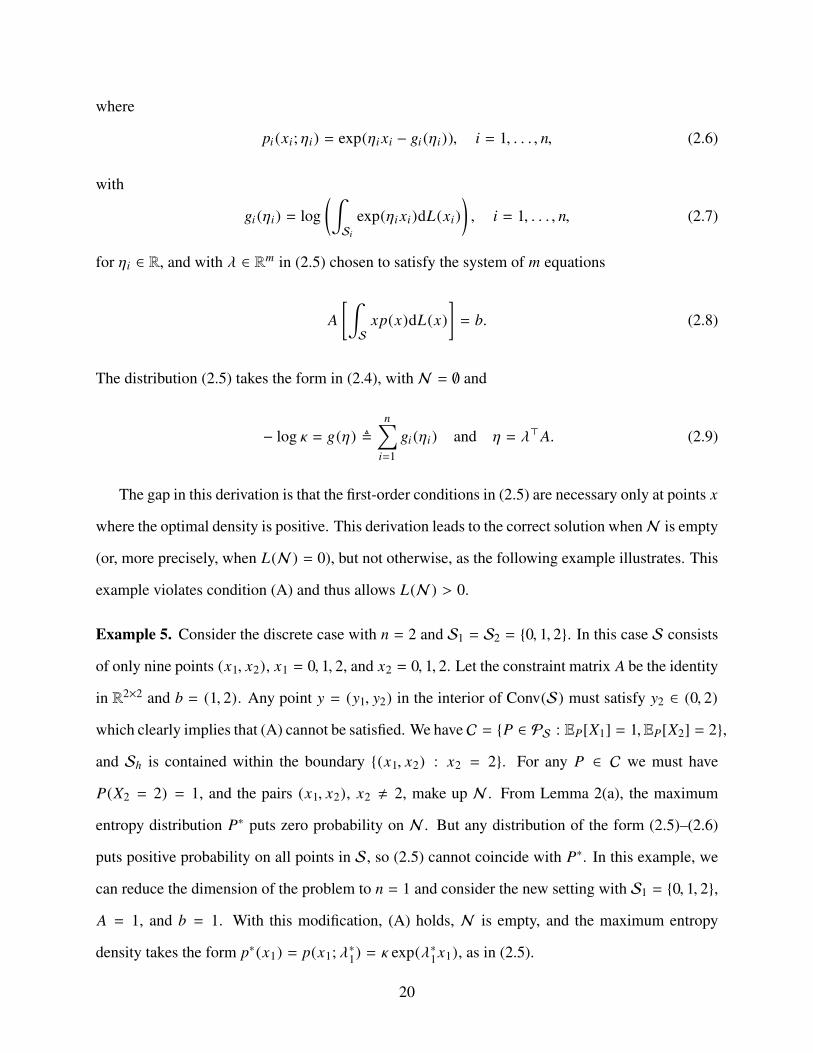
The gap in this derivation is that the first-order conditions in (2.5) are necessary only at points x
where the optimal density is positive. This derivation leads to the correct solution whenN is empty
(or, more precisely, when L(N ) = 0), but not otherwise, as the following example illustrates. This
example violates condition (A) and thus allows L(N ) > 0.
Example 5. Consider the discrete case with n = 2 and S1 = S2 = {0, 1, 2}. In this case S consists
of only nine points (x1, x2), x1 = 0, 1, 2, and x2 = 0, 1, 2. Let the constraint matrix A be the identity
in R2×2 and b = (1, 2). Any point y = (y1, y2) in the interior of Conv(S) must satisfy y2 ∈ (0, 2)
which clearly implies that (A) cannot be satisfied. We have C = {P ∈ PS : EP[X1] = 1,EP[X2] = 2},
and Sh is contained within the boundary {(x1, x2) : x2 = 2}. For any P ∈ C we must have
P(X2 = 2) = 1, and the pairs (x1, x2), x2 , 2, make up N . From Lemma 2(a), the maximum
entropy distribution P∗ puts zero probability on N . But any distribution of the form (2.5)–(2.6)
puts positive probability on all points in S, so (2.5) cannot coincide with P∗. In this example, we
can reduce the dimension of the problem to n = 1 and consider the new setting with S1 = {0, 1, 2},
A = 1, and b = 1. With this modification, (A) holds, N is empty, and the maximum entropy
density takes the form p∗(x1) = p(x1; λ∗1) = κ exp(λ∗1x1), as in (2.5).
20

When the maximum entropy distribution P∗ does satisfy the conditions (2.5), (2.6), and (2.8),
it samples the entries of each point x = (x1, . . . , xn) independently and with marginal density
pi (·; (λ∗>A)i). This property holds in more generality, the key element being the separability
(rather than the linearity) of h(·). For example, with a constraint of the form∑
i ai x2i = b we get
(2.4) but with Ax replaced by∑
i ai x2i .
Example 6 (Bipartite graphs revisited). The solution to the maximum entropy problem for bipartite
graphs with given degree sequences is discussed in Glasserman and Lelo de Larrea 2018, but the
representation (2.4) and the connection with exponential families are not considered there. The
graph is conveniently represented through its 0–1 adjacency matrix X . To match (2.4), we would
need to unravel the entries of X into a long vector, but the solution is easier to interpret through
the matrix (see Section 3.1 for more details). Uniform sampling over the full set S = {0, 1}n is
achieved by generating the entries of X as independent Bernoulli random variables with parameter
1/2. (To force some entries to be 0 or 1, we would remove the corresponding coordinate of S.)
Fixed degrees for all nodes correspond to equality constraints on the row sums and column sums of
X . Each entry Xi j appears in one row-sum constraint and one column-sum constraint; hence, the
density in (2.4) factors as a product of terms exp((si+t j )xi j ) and a normalization constant, where si
and t j are Lagrange multipliers. Assume that (A) holds and thus the setN is empty. The outcomes
Xi j = 0 and Xi j = 1 then have probabilities proportional to 1 and exp(si + t j ). Normalizing yields
a success probability of P∗(Xi j = 1) = exp(si + t j )/(1 + exp(si + t j )) , zi j . In other words, under
the maximum entropy distribution, the entries of X are independent Bernoulli random variables
with tilted parameters zi j . These parameters enforce the row-sum and column-sum constraints in
expectation. The values zi j define the maximum entropy matrix of Barvinok 2010.
In the context of graphs, such as in Example 6, the exponential form of (2.4) has received exten-
sive study under the heading of Gibbs measures, as in Dembo and Montanari 2010, or exponential
random graph models (ERGM), as introduced in Holland and Leinhardt 1981. The basic ERGM
has been extended in many directions, including the case of graphs with continuous weights treated
in Desmarais and Cranmer 2012. On the simulation side, Britton et al. 2006 use an Erdos-Rényi
21

model, which can be seen to be an ERGM (see Section 10 of Blitzstein and Diaconis 2011), with
random parameters to sample graphs with mixed Poisson degree distributions, as the size of the
network grows.
2.2.4 Conditional Uniformity
For any λ ∈ Rm, define a distribution Pλ>A with density p(x; λ>A) as in (2.4), where N is any
set having zero probability under the uniform distribution on Sh. These distributions include the
maximum entropy distribution in the discrete case (by Lemma 3) or in the continuous case if (A)
holds. Importantly, they are all uniform on the target set Sh:
Proposition 1. For any λ ∈ Rm, the density of Pλ>A, is constant on Sh, so the distribution of X
given X ∈ Sh is uniform on Sh. In the case of the maximum entropy distribution, the constant
value of the density is given by p∗(x) = exp(−H (P∗)), for all x ∈ Sh.
The first claim follows directly from the fact that for any x ∈ Sh, we may suppose x < N and
then
p(x; λ>A) = κλ exp(λ>Ax) = κλ exp(λ>b) ≡ constant, (2.10)
because h(x) = Ax − b = 0 for all x ∈ Sh. The value of the constant in the case of the maxi-
mum entropy distribution follows from part (c) of Lemma 2. Theorem 4 of Barvinok 2010 proves
the second statement of Proposition 1 for 0–1 matrices with given row sums and column sums.
Proposition 1 shows that this property holds for a broad class of problems.
In the discrete case, conditional uniformity leads to a family of acceptance-rejection methods
for sampling from Sh:
1. Generate a sample X from Pλ>A.
2. While X is not in Sh, go to 1.
3. Return X .
22

In practice, the probability that a candidate X will fall in Sh may be small, as we shall see in the
next section. We will therefore describe a sequential method in Section 2.5 that always produces a
successful draw.
2.2.5 Acceptance-rejection and comparison with the Erdos-Rényi model
Consider once again the problem of uniformly sampling graphs with fixed degree sequences.
Recall that the set of simple undirected graphs on M nodes can be expressed via n = M (M − 1)/2
possible edges with Bernoulli random variables Xi j , where i , j index the graph nodes. Let the
desired degree sequence be d = (d1, . . . , dM ). To do the sampling, a standard (naive) approach
is to generate a graph using the classic Erdos-Rényi (ER) model and to accept if it satisfies the
degree sequence; otherwise, the sample is rejected and the process repeats. The ER model samples
the n edges independently with constant probability P(Xi j = 1) , β. Any value of β ∈ (0, 1)
will give us uniform sampling on the target set. To see this, apply Proposition 1 with a constant
λER = (φ, . . . , φ), where φ = log(β/(1 − β))/2. In particular, we consider the case β∗ = d/(2n),
where d ,∑M
i=1 di. Sampling via ER with β∗ will produce graphs that, on average, have the same
fraction of edges present as the graphs in the target set.
We compare this method against acceptance rejection under the maximum entropy (ME) dis-
tribution P∗, for various graph degree sequences. The purpose of this comparison is to illustrate
how the ME method incorporates additional information into the edge-sampling probabilities. For
each method (ER or ME) and degree sequence, we simulate m = 1000 accepted graphs to estimate
acceptance probabilities; in some cases it is possible to compute the probability exactly. Due to
the conditional uniformity property of Proposition 1, we have that the acceptance probabilities are
|Sh |p(x; λ>ER A) and |Sh |p∗(x), for ER and ME, respectively, and x is any point in Sh. The ratio can
thus be computed explicitly, since the unknown factor Sh cancels. Table 2.1 reports the acceptance
probabilities under ER and ME and their ratio.
The first three degree sequences (a–c) in the table are degenerate in the sense that there is only
one graph satisfying the degree sequence. ME correctly assigns probability 0 or 1 to each edge and
23
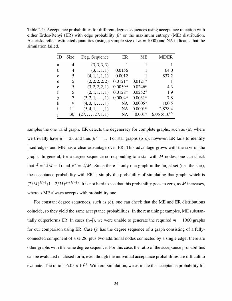
Table 2.1: Acceptance probabilities for different degree sequences using acceptance rejection witheither Erdos-Rényi (ER) with edge probability β∗ or the maximum entropy (ME) distribution.Asterisks reflect estimated quantities (using a sample size of m = 1000) and NA indicates that thesimulation failed.
ID Size Deg. Sequence ER ME ME/ER
a 4 (3, 3, 3, 3) 1 1 1b 4 (3, 1, 1, 1) 0.0156 1 64.0c 5 (4, 1, 1, 1, 1) 0.0012 1 837.2d 5 (2, 2, 2, 2, 2) 0.0121* 0.0121* 1e 5 (3, 2, 2, 2, 1) 0.0059* 0.0246* 4.3f 5 (2, 1, 1, 1, 1) 0.0128* 0.0252* 1.9g 7 (3, 2, 1, . . . , 1) 0.0004* 0.0031* 7.8h 9 (4, 3, 1, . . . , 1) NA 0.0005* 100.5i 11 (5, 4, 1, . . . , 1) NA 0.0001* 2,878.4j 30 (27, . . . , 27, 1, 1) NA 0.001* 6.05 × 1065
samples the one valid graph. ER detects the degeneracy for complete graphs, such as (a), where
we trivially have d = 2n and thus β∗ = 1. For star graphs (b–c), however, ER fails to identify
fixed edges and ME has a clear advantage over ER. This advantage grows with the size of the
graph. In general, for a degree sequence corresponding to a star with M nodes, one can check
that d = 2(M − 1) and β∗ = 2/M . Since there is only one graph in the target set (i.e. the star),
the acceptance probability with ER is simply the probability of simulating that graph, which is
(2/M)M−1(1−2/M)n−(M−1). It is not hard to see that this probability goes to zero, as M increases,
whereas ME always accepts with probability one.
For constant degree sequences, such as (d), one can check that the ME and ER distributions
coincide, so they yield the same acceptance probabilities. In the remaining examples, ME substan-
tially outperforms ER. In cases (h–j), we were unable to generate the required m = 1000 graphs
for our comparison using ER. Case (j) has the degree sequence of a graph consisting of a fully-
connected component of size 28, plus two additional nodes connected by a single edge; there are
other graphs with the same degree sequence. For this case, the ratio of the acceptance probabilities
can be evaluated in closed form, even though the individual acceptance probabilities are difficult to
evaluate. The ratio is 6.05 × 1065. With our simulation, we estimate the acceptance probability for
24

ME to be around 0.001. Clearly, the simulation for ER failed within our setup. This example again
illustrates that ME is able to discover and exploit information in degree sequences in choosing the
edge-sampling probabilities.
Our max-min result Theorem 1 will provide a simple condition ensuring that the acceptance
probability under ME is at least as large as the acceptance probability under ER, for any choice
of edge probability β. In Section A.3, we use Chernoff bounds to analyze the ME acceptance
probability when we allow some tolerance in the constraints. In dense networks, a small amount
of tolerance can substantially increase the acceptance probability.
2.2.6 Importance Sampling and Cross Entropy
We briefly contrast the maximum entropy distribution for uniform sampling with the cross
entropy method for importance sampling, while noting that these methods address different prob-
lems. As before let QU denote the uniform distribution on S, and now let Qh denote the uniform
distribution on Sh. Consider the problem of estimating QU (X ∈ Sh), the probability that X falls
in Sh when sampled uniformly from S.
To estimate this probability, the cross entropy method (see Rubinstein and Kroese 2013) looks
for a distribution P that makes D(Qh ‖ P) small, within a family of tractable distributions. In
contrast, from (2.2), we see that maximizing entropy is equivalent to minimizing D(P ‖ QU ).
Relative entropy is not symmetric, so the two problems use different objectives, as well as differing
in their comparison with QU or Qh. For fixed Q, D(· ‖ Q) and D(Q ‖ ·) are sometimes called the
forward and backward Kullback-Leibler divergence measures, respectively.
With QU as the reference measure for importance sampling, D(P ‖ QU ) measures how far the
distribution P deviates from QU , and a larger value suggests a more “aggressive” change of mea-
sure in an importance sampling procedure. By this criterion, the maximum entropy method seeks
the most conservative change of distribution in C. Given a common set of candidate distributions,
the cross entropy method will make a less conservative choice. We can make this contrast more
25

precise by noting that if P has density p, then
D(Qh ‖ P) = −H (Qh) − EQh[log p(X )]; (2.11)
in minimizing (2.11), the cross entropy method thus seeks to make the average log probability over
Sh large. In the next section, we investigate the alternative of making the minimum log probability
over Sh large and identify when the maximum entropy distribution achieves this objective.
2.3 The Max-Min Probability Distribution
We now derive a second candidate distribution to sample from Sh, based on maximizing the
minimum probability over Sh within an expanded family. The max-min objective is attractive
because it favors both uniformity and increasing the probability of the target set. We will derive
simple conditions under which the maximum entropy distribution achieves the max-min objective.
We consider an exponential family of distributions Pη on S with independent marginals pa-
rameterized by the natural parameter η ∈ Rn. This family has densities of the form
p(x; η) =n∏
i=1
pi (xi; ηi) ,n∏
i=1
exp(ηi xi − gi (ηi)), x ∈ S, (2.12)
where gi (·) is defined in equation (2.7) and η ∈ Ξ = {η ∈ Rn : gi (ηi) < +∞, i = 1, . . . , n}. The set
Ξ is the parameter space of the exponential family and in our case, since the support S is assumed
to be bounded, we have Ξ = Rn. Any distribution of the form in (2.4) withN = ∅ and any λ ∈ Rm
is a member of this exponential family with η = λ>A. In the graph setting of Section 2.2.5, so is
every Erdos-Rényi distribution.
For each distribution Pη in the exponential family (2.12), we define its minimum on Sh to be
ρ(η) , minx∈Sh p(x; η), for η ∈ Rn. The minimum is attained since in the discrete case, Sh is
finite, and in the continuous case, Sh is compact and p(·; η) is continuous. Without the condition
η = λ>A, the distributions in (2.12) need not be constant on Sh, as in Proposition 1. We define the
26

max-min probability problem as
maximizeη∈Rn
ρ(η). (2.13)
Lemma 4. log ρ(·) is concave, and thus (2.13) is a convex optimization problem.
A solution to (2.13) provides a potentially attractive sampling distribution because the max-
min objective will tend to increase the probability of Sh and favor uniformity over Sh. At first
glance, it might not be clear how to solve problem (2.13) or even to determine if the maximum
is attained. We shall see in the next section that, under certain simple conditions, the maximum
entropy distribution solves the max-min problem.
2.4 Solution of the Max-Min Problem by the Maximum Entropy Distribution
This section contains our main theoretical results for the maximum entropy distribution. Under
condition (A), we know from Lemma 2(b) that we may takeN to be empty, making the maximum
entropy distribution P∗ a member of the exponential family in (2.12): it corresponds to the natural
parameter η∗ , λ∗>A. Let y∗ be the mean vector associated with P∗, that is y∗ = EP∗[X]. The
max-min objective attained by the maximum entropy distribution takes a particularly simple form:
Proposition 2. Suppose (A) holds. Let η∗ be the natural parameter of the maximum entropy dis-
tribution P∗. Then ρ(η∗) = exp(−H (P∗)).
The identity in the proposition is a special feature of the maximum entropy distribution. The
identity does not in general hold for other distributions in (2.12) corresponding to other values of
η. This result suggests that there may be a connection between the two optimization problems.
Our main theoretical contribution establishes the connection:
Theorem 1. Suppose (A) holds. Let P∗ be the maximum entropy distribution and let y∗ be its
mean. Then P∗ is also a max-min probability distribution (that is, η∗ = λ∗>A solves problem 2.13)
if and only if y∗ ∈ Conv(Sh).
The condition on the mean vector in Theorem 1 is a restriction only in the discrete case, as the
following results shows:
27

Corollary 1. Suppose (A) holds. In the continuous case, the maximum entropy problem and the
max-min probability problem have the same solution.
Proof of Corollary 1. It is clear that y∗ ∈ Conv(S) since it is an expected value of a random
variable defined on S. In the continuous case, S is convex, so Conv(S) = S and y∗ ∈ S. Also,
P∗ ∈ C implies h(y∗) = 0. Therefore, y∗ ∈ Sh ⊂ Conv(Sh) and the result follows from Theorem 1.
�
To illustrate why the condition y∗ ∈ Conv(Sh) is needed in the discrete case, we consider a
simple example.
Example 7. Consider a discrete, 2-dimensional example with S = {0, 1, 2, 3} × {0, 1, 2}, as in
Figure 2.2. For any a > 1, the line x2 = 1 + a(x1 − 2) intersects S only at the point (2, 1),
so Sh and therefore Conv(Sh) contain only this point. The mean y∗ of the maximum entropy
distribution has y∗1 < 2 and y∗2 < 1, for all a > 1; Figure 2.2 shows the case a = 1.2. In particular,
y∗ < Conv(Sh), so the condition in Theorem 1 is violated. The max-min distribution is the one that
maximizes the mass at (2, 1); this distribution has its mean at (2, 1), and it puts strictly more mass
at (2, 1) than any other Pη . (This follows from Lemma 11 in Appendix A.4.2.) The maximum
entropy distribution is therefore not the max-min distribution.
The point y∗ can be viewed as a projection (though not the Euclidean projection) of the mean
of the uniform distribution on S (marked by the open circle at (1.5, 1) in the figure) onto the line
defined by the constraint. At a = 1, the endpoints of the dashed line in the figure are points in S
and therefore in Sh, so y∗ ∈ Conv(Sh), and P∗ becomes the max-min distribution. The mean of
the max-min distribution is thus at (2, 1) for a < 1 and at y∗ , (2, 1) for a = 1.
As this example indicates, for the two optimization problems to be equivalent in the discrete
case, we need to add some structure to the constraint function h(x) = Ax − b. In particular, it
suffices to assume the matrix A to be totally unimodular (TUM) and the vector b to be integer.
Recall that a matrix B is said to be TUM if every square sub-matrix of B has determinant equal to
0, 1, or −1.
28

y*
Figure 2.2: Sh is the intersection of the line x2 = 1+a(x1−2) with the set S = {0, 1, 2, 3}×{0, 1, 2}.With a > 1, the maximum entropy mean y∗ is not in Conv(Sh), and P∗ is not the max-mindistribution, which has its mean at (2, 1).
Corollary 2. Suppose (A) holds. Assume that in the constraint function h(x) = Ax−b, A is a TUM
matrix and b is an integer vector. Then, in the discrete case, the maximum entropy distribution
solves the max-min probability problem.
The TUM condition applies, in particular, to the case of bipartite graphs in Example 1. Fixing
the degrees of the nodes is equivalent to fixing the row sums and column sums of the adjacency
matrix. These constraints (along with possible upper and lower bounds on individual entries)
define a transportation polytope and are well-known to be TUM; see, for example, Theorem 13.3
of Papadimitriou and Steiglitz 1998. As a consequence, we have the following result. We are not
aware of any similar results in the literature or any other results that consider max-min probabilities
over random graphs.
Corollary 3. Among all distributions that sample the edges of a bipartite graph with independent
(but not necessarily identically distributed) Bernoulli random variables, the maximum entropy
distribution maximizes the minimum probability over all graphs with the given degree sequences.
In the example of Figure 2.2, the constraint matrix A is simply the scalar a, and the TUM
condition is satisfied if a ∈ {−1, 0, 1}. In these three cases, the endpoints of the dashed line in
the figure are in S, and y∗ is contained in Conv(Sh). But the TUM condition is not in general
necessary. For example, if we replace the constraint with x2 = 2x1/3, we get Sh = {(0, 0), (3, 2)},
and y∗ = (1.5, 1) ∈ Conv(Sh).
29

We conclude this section by revisiting the cross entropy method discussed in Section 2.2.6.
Consider the problem of minimizing D(Qh ‖ Pη ) over η ∈ Rn. Let y denote the mean of the
uniform distribution over Sh. For the next result, we need to modify (A) to the stronger condition
(A′) The target set Sh has a point in the interior of Conv(S).
Proposition 3. Suppose (A′) holds. The cross entropy objective D(Qh ‖ Pη ) is minimized at the
unique η× ∈ Rn for which the mean of Pη× is y. If y∗ ∈ Conv(Sh) and η× , η∗, then ρ(η×) < ρ(η∗)
and the density of Pη× is not constant on Sh.
The last statement implies that except in cases where the cross entropy distribution is max-min
optimal, it does not provide the conditional uniformity in Proposition 1. As noted at the end of
Section 2.2.6, the cross entropy objective maximizes the average log probability, rather than the
minimum log probability, over the target set.
Example 8 (Example 7 revisited). Consider again the example in Figure 2.2. For any value of a,
the cross entropy distribution has its mean at y = (2, 1). As a varies, we therefore get a range of
outcomes: for a > 1, the cross entropy distribution is max-min optimal and the maximum entropy
distribution is not; at a = 1, the maximum entropy distribution is max-min optimal and the cross
entropy distribution is not; in the limiting case a = +∞, corresponding to a vertical constraint at
x1 = 2, both the maximum entropy and cross entropy distributions are max-min optimal.
2.5 Sequential Algorithm for the Discrete Case
In Section 2.2.4 we introduced a simple acceptance-rejection algorithm to sample uniformly
from Sh. However, we saw in Section 2.2.5 that, in practice, the acceptance probability of a sample
X will be small, even if we use the maximum entropy distribution P∗ as the sampling distribution.
In this section, we describe a sequential algorithm that will always produce a valid sample X ∈ Sh.
The cost of this algorithm will be the loss of the uniformity of the samples. We correct for the loss
of uniformity through importance sampling weights.
30

The idea behind the sequential algorithm is simple: First compute the maximum entropy dis-
tribution, but, instead of sampling all entries at the same time, such as in the one-shot method of
Section 2.2.4, sample only the first entry. Once that entry is fixed, consider the remaining sub-
problem with one less entry (after adjusting the linear constraints) and re-compute the maximum
entropy distribution. Continue until all entries have been sampled. This sequential algorithm is an
extension of the one proposed in Glasserman and Lelo de Larrea 2018 for bipartite graphs. We
refer the reader to that paper for a simple example of how the algorithm samples bipartite graphs
with fixed degree sequences.
To formulate our algorithm, we need to introduce some notation. We denote an instance of our
maximum entropy problem as P , P (n, A, b, {Si}ni=1), where n is the dimension of the problem, A
and b are the matrix and vector of the affine mapping h(x) = Ax−b, and the sets Si are the supports
for each entry. Recall that our goal is to sample points of S = Xni=1Si that satisfy h(x) = 0. Our
algorithm will proceed by fixing values for coordinates x1, . . . , xn sequentially. Starting from the
original instance P (0) = P, we will generate x1; fixing this coordinate yields a subinstance P (1)
of the original problem with n − 1 coordinates remaining. As we proceed, this process creates
a nested sequence of problem instances P (1), . . . ,P (n). We will write P (i) = Hxi (P(i−1)), i =
1, . . . , n, for the operation that creates the subinstance P (i) from fixing xi in subinstance P (i−1).
The transformation Hxi updates the constraints in light of the value fixed for coordinate xi. More
explicitly, Hξ (P (n, A, b, {Si}ni=1)) = P (n − 1, A, b, {Si}
ni=2), where A is the same as A but with the
first column A·1 removed, and b = b − A·1ξ.
We will also assume that given any problem sub-instance P, we are able to determine whether
its underlying target set Sh is non-empty. This is done by invoking a feasibility oracle that we
denote O. We have that O(P) = TRUE if Sh , ∅ and O(P) = FALSE, otherwise. We will assume
that O(P (0)) = TRUE, as we did in Section 2.1. For each sub-instance P (i), we let P(i)∗ denote
its maximum entropy distribution. Observe that for some x ∈ S, P(i)∗ may not be well-defined.
However, O(P (i)) = TRUE is a sufficient condition (although not necessary) for the existence and
uniqueness of P(i)∗ as seen in Lemma 1. Note that the terminal sub-instance P (n) is a degenerate
31

case of dimension zero and we define O(P (n)) = TRUE if and only if b(n) , b −∑n
i=1 A·i xi = 0;
this condition is equivalent to Ax = b, which means that we have found a valid point x ∈ Sh.
The sequential algorithm for sampling from Sh is described in Algorithm 1. The algorithm
Algorithm 1 Sequential algorithm for sampling from Sh
1: input problem instance P (0) = P (n, A, b, {Si}ni=1) and oracle O
2: require O(P (0)) = TRUE3: initialize x ∈ Rn as x ← (0, . . . , 0), πx ← 1, τx ← 1, and χx ← 14: for i = 1, . . . , n do5: compute P(i−1)∗ by solving the maximum entropy problem6: initialize τ(i,1)
x ← 1 and τ(i,2)x ← 1
7: for j = 1, 2 do8: generate ξ from p(i−1)∗
i (ξ)9: update xi ← ξ
10: compute P (i) = Hxi (Pi−1)
11: if O(P (i)) = FALSE then update τ(i, j)x ← τ
(i, j)x + 1 and go to line 8
12: end for13: update πx ← πx×p(i−1)∗
i (xi), τx ← τx× (τ(i,1)x +τ(i,2)
x )/2, and χx ← χx×1/(τ(i,1)x +τ(i,2)
x −1)14: end for15: return x, πx , τx , and χx
starts by finding the initial maximum entropy distribution P(0)∗. It then simulates the first compo-
nent x1. Once x1 has been fixed, we update the constraints of the problem accordingly and are left
with a sub-instance of the problem of dimension n−1. If this new problem P (1) is deemed feasible
by O, we continue to the next entry. If not, we go back to the step of simulating x1. We repeat
the process until all of the entries have been simulated and we output the vector x. Besides the
point x, Algorithm 1 returns the quantities πx , τx , and χx . We will use these quantities to compute
estimators for the probability that the algorithm simulates x and to compute importance sampling
weights.
Observe that the marginal density p(i−1)∗i is readily available to us by (A.1) (see Appendix A.2)
and that it is either a (discrete) exponential distribution defined on Si with parameter λ (i−1)∗>A·i
or a Dirac measure that assigns probability one to either 0 or si. In either case, the simulation can
be done easily. We also draw attention to the order in which the entries are simulated (which in
Algorithm 1 is simply from 1 to n). This order has been assumed for the sake of simplicity, but it
32

is completely arbitrary and can be modified to any fixed or adaptive order. In fact, in Section 2.5.4
we will propose an adaptive scheme to improve the uniformity of the samples. In Section 2.5.2 we
also address the assumption of the existence of the oracle O, since it will determine the practicality
of Algorithm 1.
2.5.1 Properties of the Sequential Algorithm
We first show that Algorithm 1 always runs to completion and that the output is indeed in Sh.
Proposition 4. Algorithm 1 always terminates and the output x is in the target set Sh.
We now show that any point x ∈ Sh can be simulated by Algorithm 1 with positive probability
at least equal to πx =∏n
i=1 p(i−1)∗i (xi). We also identify an unbiased estimator for this probability
and its inverse.
Proposition 5. Let px be the probability that Algorithm 1 generates x. Then,
(a) px ≥ πx > 0 for all x ∈ Sh,
(b) πxτx is an unbiased estimator of px , and
(c) χx/πx is an unbiased estimator of 1/px .
Observe that the lower bound πx depends on the outcome x ∈ Sh. We now identify a universal
lower bound on πx and thus automatically on px . This lower bound relies on the idea that entropy
should decrease as we fix coordinates. The following lemma bounds the resulting entropy decrease
from below.
Lemma 5. Let P be an instance of the maximum entropy problem and let ξ ∈ S1. Consider the sub-
instance P (1)ξ , Hξ (P). Assume that O(P (1)
ξ ) = TRUE. Then, H (P∗) − H (P(1)∗ξ ) ≥ − log p∗1(ξ).
This lemma leads to a lower bound for px using the entropy H (P∗):
Proposition 6. For all x ∈ Sh, px ≥ πx ≥ exp(−H (P∗)).
33

2.5.2 Comments on the Feasibility Oracle
Algorithm 1 assumes that we have access to the feasibility oracle O which, given a problem
instance P, determines if its target set Sh is non-empty. This amounts to determining if there is
an integer point which satisfies certain linear constraints. When the number of variables n is fixed,
Lenstra 1983 proposed an algorithm for solving this problem in polynomial time when A and b
have integer values. This algorithm is theoretical in nature and might not be competitive for real-
life applications. We now show that by adding some structure on A and b, the oracle O becomes
simpler to implement.
If the matrix A is TUM and b is integer, the vertices of the polytope
Conv(S)h , {y ∈ Conv(S) : Ay = b} ={y ∈ Rn : Ay = b, 0 ≤ y ≤ s
}are integer (see the proof of Corollary 2). This property also holds for certain generalizations of
TUM matrices with rational entries. Therefore, it suffices for O to determine if there is a point (not
necessarily integer) which satisfies the constraints. This problem is equivalent to the feasibility
problem in standard linear programming and can be solved efficiently using, for instance Phase
I of the two-phase simplex algorithm (see, for example, Section 3.5 of Bertsimas and Tsitsiklis
1997).
If we restrict ourselves to the binary case (still with A TUM and b integer), it is not even
necessary to call O. Indeed, during the execution of Algorithm 1, it is always the case that
O(P (i)) = TRUE (that is, we never reject P (i)). This result follows immediately from the fol-
lowing lemma.
Lemma 6. Let P be an instance of the binary maximum entropy problem with A TUM and b
integer. Suppose that O(P) = TRUE. Let ξ ∈ {0, 1} and consider the sub-instance P (1)ξ , Hξ (P).
Then, O(P (1)ξ ) = TRUE, if p∗1(ξ) > 0.
In this case, we also clearly have that τx = 1 with probability one which implies that px = πx .
Thus, the algorithm outputs the exact probability of generating x ∈ Sh and not just a lower bound
34

or an unbiased estimator.
We argued in Section 2.4 that the case of bipartite graphs with fixed degree sequences (Exam-
ple 1) satisfies the TUM condition. Then, by Lemma 6, we do not need call to program or call O
when sampling bipartite graphs with Algorithm 1. In contrast, while sampling simple undirected
graphs with a fixed degree sequence fits in our binary setting, this problem does not have a TUM
matrix A. Empirically speaking, however, we were able to implement Algorithm 1 for undirected
graphs without an oracle O and still get valid graphs (see Section 3.5). This suggests that Lemma 6
might hold for more general binary instances although we do not make any formal claims in this
regard.
In the graph setting, O(P (0)) = TRUE is equivalent to the graphicality of a degree sequence.
A degree sequence is graphical if there exists a graph satisfying the degree sequence. For bipartite
graphs, the well-known Gale-Ryser theorem gives a necessary and sufficient condition for a degree
sequence to be graphical. For the statement of this theorem and newer sufficient graphicality
conditions, we refer the reader to Burstein and Rubin 2017. Additionally, several algorithms that
assess graphicality by constructing a feasible graph have been proposed. For instance, see the
algorithms for directed graphs in Kleitman and Wang 1973. It may be possible to treat the general
problem of constructing a feasibility oracle as a problem of machine learning on graphs and draw
on the related literature, as in Hamilton et al. 2018.
2.5.3 Non-Uniformity of the Sequential Algorithm and Importance Sampling
We have shown that Algorithm 1 will always simulate a point x in the target set Sh (and
thus a point that satisfies the constraint h(x) = 0). However, the sampling scheme provided by the
algorithm is not uniform on Sh. For a simple counterexample in the binary case, we refer the reader
to Section 3.1 of Glasserman and Lelo de Larrea 2018. In fact, for many applications, the goal is
to compute expectations with respect to the uniform distribution on Sh. In other words, we are
interested in estimating θ , EQh[ f (X )], where f (·) is a function of interest and the expectation is
taken with respect to the uniform distribution onSh. For example, by letting f ≡ 1, we can estimate
35
the number of points in the target set |Sh | (see Chen et al. 2005 and Blitzstein and Diaconis 2011).
Also, in the context of graphs, f (·) can be one of several metrics that measure different graph
properties, such as clustering, complexity, fitness, and other motifs Saracco et al. 2015. Finally, as
discussed in Glasserman and Young 2016, given a random instance of an inter-bank network, one
can evaluate various measures of systemic risk f (·) and then average over multiple draws to get
the average risk measure over networks in Sh.
Even with a non-uniform sample, we can still estimate these expectations using importance
sampling to correct the non-uniformity. The importance weight for any x ∈ Sh is wx = 1/(|Sh |px) ∝
1/px , where px > 0 is the probability that x will be simulated by Algorithm 1. This weight cor-
rects for non-uniformity because E[wX f (X )
]= θ, if X = x with probability px . Recall that
the probability px is not calculated by Algorithm 1; however, by Proposition 5(c), we have that
wx = χx/(|Sh |πx) is an unbiased estimator of wx . To estimate θ, we can then use Algorithm 1
to simulate a random sample X1, . . . , Xm and use as estimator θ = (1/m)∑m
j=1 wX j f (X j ). The
estimator θ is unbiased since E[wX f (X )
]= E
[E
[wX f (X ) | X
] ]= E
[E [wX | X] f (X )
]=
E[wX f (X )
]= θ, where the expectations are taken with respect to the distributions determined
by Algorithm 1. In most instances of interest the quantity |Sh | is unknown, and thus θ cannot be
computed explicitly. In this case, one can use the modified estimator (as in Blitzstein and Diaconis
2011) θ =∑m
j=1 wX j f (X j )/(∑m
k=1 wXk), which can be computed since the unknown constant factor
1/|Sh | cancels. Being a ratio estimator, θ is biased, but it is consistent as m → ∞.
2.5.4 An Adaptive Order Rule for the Sequential Algorithm
Algorithm 1 generates the coordinates xi in a fixed order, from i = 1 to n. But the resulting
importance sampling weights depend on the order in which the coordinates are generated because
the probabilities px depend on the order. We would like the weights to be as uniform as possible,
so we develop an adaptive rule that selects the next coordinate to be generated based on the values
of the coordinates already generated. We propose the following modification to Algorithm 1:
Definition 1 (Most-uniform adaptive order rule). At each iteration i, after computing P(i−1)∗, select
36

from the remaining n−i+1 components the one with natural parameter η (i−1)∗j = λ (i−1)∗>A· j closest
to 0.
Observe from the definition of the exponential family in (2.12) that fixing η j to 0 gives us
a uniform distribution on Sj . The rule given above says that the next coordinate generated by
Algorithm 1 should be the component that is “closest" to uniform on Sj under the maximum
entropy distribution P(i−1)∗. We expect that the most-uniform adaptive order rule will give us
better importance sampling weights in practice (see Section 3.5 for this analysis). This adaptive
rule is a heuristic that we derive in detail in Section A.6.2.
2.6 A Monotonicity Property of the Max-Min Probability
The max-min distribution defined by (2.12)–(2.13) generates all coordinates in one shot; Al-
gorithm 1 generates all coordinates sequentially, updating the probabilities at each step. We can
combine these ideas by generating k coordinates from one distribution and then generating the
remaining n − k coordinates in a single shot from the max-min distribution determined by the first
k coordinates. In this section, we prove that, for a general class of such two-stage sampling pro-
cedures, the max-min probability is increasing in k. The details of this analysis can be found in
Section A.6.
To formulate the monotonicity result, consider the following two-stage approach to sampling
points from a discrete Sh. In the first stage we simulate the first k (out of n) entries xk =
(x1, . . . , xk ) using an arbitrary distribution q(·). Denote the simulated entries by xk = ξ. In
the second stage we simulate the remaining n − k entries xn−k = (xk+1, . . . , xn) independently
using the exponential distribution p(xn−k ; ηξ ) defined in (2.12). The parameter ηξ may depend on
the value xk = ξ generated in the first stage. These two simulation stages define a new family of
distributions on S. Let ρ(k)∗ denote the maximum over such two-stage distributions of the min-
imum probability over S, for k = 0, . . . , n. We considered the case k = 0 in Sections 2.3 and
2.4. In Section A.6, we extend that analysis to arrive at the following monotonicity result for these
max-min probabilities:
37

Proposition 7. Let P (n, A, b, {Si}ni=1) be a discrete instance with A TUM and b integer. Then,
exp(−H (P∗)) = ρ(0)∗ ≤ ρ(1)∗ ≤ . . . ≤ ρ(n)∗ = 1/(|Sh |).
If (A) holds, this result also holds if the second-stage sampling follows the maximum entropy
distribution, generalizing Corollary 2. When k = 0 we recover the original (one-stage) max-min
result from Section 2.4, and when k = n we have the uniform distribution on the target set Sh.
As we increase k, we increase the probability of sampling from Sh, while maintaining conditional
uniformity. However, solving the max-min problem for a higher k becomes increasingly difficult
due to the exponential increase in possible values during the first stage; see Section A.6 for more
details. We also show in Section A.6 that the most-uniform adaptive order rule can be derived as a
heuristic from the max-min probability distribution with k = 1.
38

Chapter 3: Sequential Random Graph Simulation
3.1 Weighted Bipartite Graph Simulation
In this section we describe in more detail the simulation of weighted bipartite graphs with
degree constraints introduced in Examples 1, 2, and 6. We restrict ourselves to the discrete case.
Consider a weighted bipartite graph with two node sets of sizes M and N , respectively. We
represent such a graph using its adjacency matrix X ∈ RM×N . The non-negative entry xi j ∈ Si j
represents the weight of the edge between node i of the first class of nodes and node j of the second
class of nodes. The rows of X correspond to the nodes of the first node set of the graph and the
columns to the nodes of the second node set. If we want to fix any weight to zero, we can just
remove the index (i, j).
Degree constraints can be enforced using affine functions. A degree constraint on node i of
the first node set can be written as the row constraint∑N
j=1 xi j = ri, i = 1, . . . , M , and a degree
constraint on node j of the second node set can be written as the column constraint∑M
i=1 xi j = c j ,
j = 1, . . . , N . Observe that any feasible degree sequence r = (r1, . . . , rM ) and c = (c1, . . . , cN )
must satisfy∑M
i=1 ri =∑N
j=1 c j .
We are interested in uniformly sampling from the set of all graphs X that satisfy the degree
sequences (r, c). To express this set of weighted graphs in the terms of Section 2.1, we rearrange
the matrix X into a long vector x ∈ Rn, with n = M N , and with entries xk = xi j , where k =
(i − 1)N + j, for i = 1, . . . , M and j = 1, . . . , N . Let eN be the vector of ones in RN , 0N the
vector of zeros in RN , and IN the identity matrix in RN×N . We define the matrix of row constraints
39
Arow ∈ RM×n as
Arow =
e>N 0>N · · · 0>N
0>N e>N · · · 0>N...
.... . .
...
0>N 0>N · · · e>N
,
the matrix of column constraints Acol ∈ RN×n as
Acol =
[IN IN · · · IN
],
and the matrix Agr ∈ R(M+N )×n as
Agr =
Arow
Acol
.
If we let bgr = (r, c) ∈ RM+N , and hgr(x) = Agrx − bgr, then it is clear that the degree constraints
are equivalent to imposing the affine constraint hgr(x) = 0. Therefore, the graph setting can be
expressed as the problem instance P (n, Agr, bgr, {Si}ni=1). It follows then that, if we want to simulate
graphs with degree constraints, we can readily do so using Algorithm 1.
3.1.1 Maximum Entropy Distribution for the Graph Case
Given the special structure of the constraint matrix Agr, we characterize the maximum entropy
distribution P∗ in the graph setting. If (A) holds, then there exists λ∗ ∈ RM+N such that P∗ =
Pλ∗>Agr . This implies that P∗ samples the graph weights independently with distribution equal to
pk (xk ; (λ∗>Agr)k ) = exp((λ∗>Agr)k xk − gk (λ∗>Agr)k )), for k = 1, . . . , n. Since Agr has M row
constraints and N column constraints, we can decompose the vector λ∗ ∈ RM+N into λ∗ = (s∗, t∗),
with s∗ ∈ RM and t∗ ∈ RN . Therefore, given an edge (i, j) and its corresponding index k =
(i − 1)N + j, we have (λ∗>Agr)k = (s∗>Arow + t∗>Acol)k = s∗i + t∗j and we get that the probability
distribution of edge (i, j) is pi j (xi j ; s∗i , t∗j ) = exp((s∗i + t∗j )xi j − gi j (s∗i + t∗j )), with gi j (·) , gk (·), for
i = 1, . . . , M and j = 1, . . . , N .
40

We argued before that Agr is TUM and it is clear that we must require bgr to be integer in
order for the problem to be feasible. Therefore, as a consequence of Corollary 2, we have that the
maximum entropy distribution is also a max-min distribution in the graph case.
It remains only to determine the appropriate vectors s∗ and t∗. As previously seen for the
general case in (2.8), s∗ and t∗ must satisfy the system of M + N equations AgrEP∗[X] = bgr. This
system of equations can be rewritten as
N∑j=1
EP∗[Xi j] = ri, i = 1, . . . , M,
M∑i=1
EP∗[Xi j] = c j, j = 1, . . . , N,
or equivalently, in view of (A.4), as
N∑j=1
g′i j (s∗i + t∗j ) = ri, i = 1, . . . , M,
M∑i=1
g′i j (s∗i + t∗j ) = c j, j = 1, . . . , N,
(3.1)
where g′i j (·) is the derivative of gi j (·). Therefore, finding the maximum entropy distribution
amounts to finding a solution (s∗, t∗) of system (3.1), which can be done numerically. Notice that
the solution (s∗, t∗) is not unique since, for any ε ∈ R, the vector formed by s∗i + ε, i = 1, . . . , M
and t∗j − ε, j = 1, . . . , N is another solution. Observe that there is a coupling between s and t via
the functions g′i j (·). This coupling complicates the process of solving (3.1) slightly, but it can be
circumvented by using the iterative method proposed in Algorithm 2.
This algorithm starts by assigning initial values s(0) = 0 ∈ Rm and t (0) = 0 ∈ Rn. For the kth
iteration, given s(k−1) and t (k−1), we first do a row update by finding the vector s(k) that satisfies
the row constraintsN∑
j=1
g′i j
(s(k)
i + t (k−1)j
)= ri i = 1, . . . , M . (3.2)
41

Algorithm 2 Iterative method for solving the maximum entropy system in the graph case
1: input degree sequences r ∈ RM+ and c ∈ RN
+
2: initialize s ← 0 ∈ RM and t ← 0 ∈ RN
3: repeat4: for i = 1, . . . , M do5: find σi ∈ R such that
∑Nj=1 g
′i j (si + σi + t j ) = ri
6: set si ← si + σi7: end for8: for j = 1, . . . , N do9: find τj ∈ R such that
∑Mi=1 g
′i j (si + t j + τj ) = c j
10: set t j ← t j + τj11: end for12: until convergence of s and t13: return s and t
The pair (s(k), t (k−1)) satisfies the row constraints of (3.1), but probably not the column constraints.
We then do a column update by finding the vector t (k) that satisfies the column constraints
M∑i=1
g′i j
(s(k)
i + t (k)j
)= c j j = 1, . . . , N . (3.3)
The pair (s(k), t (k)) satisfies the column constraints of (3.1), but probably not the row constraints.
We repeat this process until the convergence of s(k) → s∗ and t (k) → t∗. The advantage of this
algorithm is that both the row update (3.2) and the column update (3.3) may be done in parallel,
and each individual update for either s(k)i or t (k)
j amounts to solving a non-linear equation in R.
This is simpler than trying to solve the coupled system (3.1) simultaneously. We now show that
Algorithm 2 converges to a desired vector (s∗, t∗).
Proposition 8. Assume that (A) holds. Then Algorithm 2 converges to (s∗, t∗), a solution of (3.1).
The proof can be found in Appendix B.1. Algorithm 2 is in the same spirit as the well-known
Sinkhorn algorithm (also known as RAS or IPFP algorithm) for matrix scaling (see, for instance,
the survey by Idel 2016). In fact, the convergence of the Sinkhorn algorithm may be shown using
exactly the same result that we use for the proof of the convergence of Algorithm 2 (see Csiszar
1975).
42

3.2 Random Bipartite Graphs as Random Adjacency Matrices
As a particular case, we represent bipartite or directed graphs (without weigths) using 0–1
matrices. These matrices can be interpreted as the adjacency matrices of the underlying graph.
Following the notation of Barvinok 2010, let r = (r1, r2, . . . , rM ) and c = (c1, c2, . . . , cN ) be the
sum of the rows and columns of the matrix respectively. For bipartite graphs, r and c represent the
degree sequences of the first and second disjoint sets of vertices. On the other hand, for directed
graphs, r and c represent the out-degrees and in-degrees of the vertices. Since every edge of the
graph contributes one unit to both r and c, it is necessary to have∑M
i=1 ri =∑N
j=1 c j . Furthermore,
we clearly must have 0 < ri ≤ N and 0 < c j ≤ M . For the case of directed graphs, we must
impose M = N .
Suppose also that we wish to force the exclusion of some edges of the graph. For this purpose,
let W = (wi j ) with wi j ∈ {0, 1} be a pattern matrix. If a particular edge is to be excluded, we set the
corresponding wi j to 0 and, otherwise, to 1. Observe that in the directed graph case, the elements
of the diagonal correspond to loops. If we wish to exclude graphs that contain loops, we can do so
by making the diagonal elements wii = 0.
Given the degree sequences r and c, and the pattern matrix W , we now define the set of 0–1
matrices with such degrees and assigned zeros.
Definition 2. Σ(r, c; W ) is the set of all M × N matrices x = (xi j ) such that∑N
j=1 xi j = ri for all i,∑Mi=1 xi j = c j for all j, xi j ∈ {0, 1}, and xi j = 0 if wi j = 0. If wi j = 1 for all i and j we denote it
Σ(r, c).
In terms of the notation introduced in Chapter 2 and Section 3.1, this set of matrices is the target
set defined by the linear constraints imposed by the fixed degree requirements, that is, Σ(r, c; W ) ≡
Shgr . We also need to relax the integrality constraint of Σ(r, c; W ) and work with the following
polytope.
Definition 3. P (r, c; W ) is the set of all M × N matrices y = (yi j ) such that∑N
j=1 yi j = ri for all
i,∑M
i=1 yi j = c j for all j, yi j ∈ [0, 1], and yi j = 0 if wi j = 0. If wi j = 1 for all i and j we denote it
43

P (r, c).
In terms of the notation introduced in Chapter 2 and Section 3.1, this set of matrices is the points
in the convex hull of the support that satisfy the graph linear constraints, that is, P (r, c; W ) ≡
Conv(S)hgr . We interpret the yi j as the probability that the edge (i, j) is present in the graph
(assuming independent edges). The row and column sum constraints on y imply that a graph
sampled with these probabilities has the correct expected degree sequences. We need to ensure
that the correct degree sequence holds with probability one.
We now restate the maximum entropy problem (2.3) for this particular case.
3.2.1 Maximum Entropy Problem and its Dual
For ξ ∈ [0, 1] we define the entropy function as
h(ξ) = ξ log(
1ξ
)+ (1 − ξ) log
(1
1 − ξ
).
It is a strictly concave function with h(0) = h(1) = 0. The derivative is h′(ξ) = log(1− ξ)− log(ξ)
and therefore h′(0+) = ∞ and h′(1−) = −∞. For y in P (r, c; W ) we define the entropy function as
H (y) =∑
i j
h(yi j ).
Assuming that condition (A) holds, since H is a strictly concave function it attains a unique
maximum at some y∗ = y∗(r, c; W ). That is, the maximum entropy matrix y∗ is the solution to
maximizey
H (y)
subject to y ∈ P (r, c; W ).(3.4)
Observe that the number of variables of the problem is M × N , which may be large for certain
applications. Therefore, in practice, it is more convenient, as in Barvinok 2010, to work with the
44

unconstrained dual problem which is
minimizes,t
G(s, t) , −M∑
i=1
risi −
N∑j=1
c jt j +∑
i j
log(1 + wi jesi+t j
). (3.5)
This problem has only M + N variables. We then recover the maximum entropy matrix y∗ by
setting
y∗i j =es∗i+t∗j
1 + es∗i+t∗j,
whenever wi j = 1 and y∗i j = 0 otherwise.
3.3 Sequential Algorithm for Bipartite or Directed Graphs
Given degree sequences r and c, the objective is to generate a random matrix x ∈ Σ(r, c; W ),
assuming that this set is non-empty. Our algorithm is described in Algorithm 3. This algorithm
can be derived from the more general Algorithm 1 when applied in the 0–1 matrix context.
Algorithm 3 Sequential algorithm for sampling from Σ(r, c; W )1: input: r , c, and W2: verify Σ(r, c; W ) non-empty3: initialize x ← 0, and px ← 14: compute y∗ (r, c; W )5: for all (i, j) do6: set xi j ← 1 with probability y∗i j7: if xi j = 1 then8: set px ← px ∗ y
∗i j
9: set ri ← ri − 110: set c j ← c j − 111: else12: set px ← px ∗ (1 − y∗i j )13: end if14: set wi j ← 015: compute y∗ (r, c; W )16: end for17: return x and px
45

Observe that in line 2, the algorithm verifies that Σ(r, c; W ) has at least one element. If we
have that wi j = 1 for all i and j, this can be done quickly using the criterion given by the Gale-
Ryser theorem (see, for instance, Gale 1957). It suffices to check that∑M
i=1 ri =∑N
j=1 c j and that∑kj=1 c j ≤
∑Mi=1 min(ri, k), for all k = 1, 2, . . . , N .
The algorithm starts with an empty graph x = 0 and an initial pattern W . In the case of bipartite
graphs and directed graphs when loops are permitted, W = (wi j ) has all entries equal to 1. If we
exclude loops, then we set diagonal wii = 0. The algorithm then sequentially adds edges at random
using the maximum entropy matrix y∗. At each step, if edge (i, j) is added to x, we reduce the
corresponding ri and c j by one. If the edge is not added, we leave the degree sequences intact.
In either case, we update the pattern by setting wi j = 0. This will reduce the polytope of feasible
matrices to a subset where the presence of edge (i, j) is never allowed. Finally, we update y∗ with
the new degree sequences and pattern. At the end, we return the matrix x. In the next section, we
show that this matrix is always in Σ(r, c; W ). The algorithm also computes the probability px of
generating this particular matrix x. Observe from lines 8 and 12 that
px =∏
i j
(xi j y
∗i j + (1 − xi j )(1 − y∗i j )
).
In this expression, the y∗i j do not belong to the same maximum entropy matrix. Each one is an
element of its corresponding matrix y∗ computed in line 15.
3.3.1 Illustration of the Algorithm
To better explain our algorithm, we present a simple example. Consider the bipartite graphs
with m = n = 3 and r = c = (1, 1, 2). It is easy to see that, in this case, there are five graphs
consistent with the constraints, so |Σ(r, c) | = 5. Figure 3.1 presents one realization of Algorithm
3.
In Step 1 of Figure 3.1, we start with the empty graph x = 0 and a temporary graph probability
of px = 1. We compute the maximum entropy matrix y∗ and focus on the first potential edge
46

(1)
x = *.,
0 0 00 0 00 0 0
+/-
y∗ =*.,
0.22 0.22 0.570.22 0.22 0.570.57 0.57 0.86
+/-
r = (1, 1, 2)
c = (1, 1, 2)
px = 1
W = *.,
1 1 11 1 11 1 1
+/-
B1
0
B2
0
B3
0
A1
0
A2
0
A3
0
(2)
x = *.,
0 0 00 0 00 0 0
+/-
y∗ =*.,
0 0.32 0.680.32 0.18 0.50.68 0.5 0.82
+/-
r = (1, 1, 2)
c = (1, 1, 2)
px = 1 − 0.22
W = *.,
0 1 11 1 11 1 1
+/-
B1
0
B2
0
B3
0
A1
0
A2
0
A3
0
(3)
x = *.,
0 1 00 0 00 0 0
+/-
y∗ =*.,
0 0 00 0 11 0 1
+/-
r = (0, 1, 2)
c = (1, 0, 2)
px = (1 − 0.22) × 0.32
W = *.,
0 0 11 1 11 1 1
+/-
B1
0
B2
1
B3
0
A1
1
A2
0
A3
0
(4)
x = *.,
0 1 00 0 11 0 1
+/-
y∗ =*.,
0 0 00 0 00 0 0
+/-
r = (0, 0, 0)
c = (0, 0, 0)
px = (1 − 0.22) × 0.32 ≈ 0.25
W = *.,
0 0 00 0 00 0 0
+/-
B1
1
B2
1
B3
2
A1
1
A2
1
A3
2
Figure 3.1: Realization of Algorithm 3 with m = n = 3 and r = c = (1, 1, 2).
(connecting A1 and B1). To decide if the edge will be generated, we generate a Bernoulli random
variable X1 with probability p = y∗11 = 0.22. In this particular realization, X1 = 0 and thus the
edge is not generated.
In Step 2, we update px to be px ← px ∗ (1 − y∗11) since the previous edge was not generated.
We compute y∗ and consider the next edge (connecting A1 and B2). We simulate a Bernoulli X2
with probability p = y∗12 = 0.32. This time X2 = 1 and the edge is generated.
In Step 3, the graph x now contains the edge generated in the previous step and we update px to
be px ← px ∗ y∗12, since the previous edge was generated. After computing y∗, observe that all its
entries are either 0 or 1. This means that, given the previous edges that we have decided to either
47

include or not, there is only one possible graph left that satisfies the degree sequences. The edges
that need to be added to x are the ones where y∗i j = 1.
Step 4 presents the output graph x and its corresponding probability of being generated by
Algorithm 3. Notice that px = 0.25 , 0.2 = 1/|Σ(R,C) |. We conclude that, in general, the
algorithm does not sample uniformly from Σ(r, c). However, if uniform samples are required, it is
possible to use importance sampling weights as discussed in Section 3.3.3.
Observe that in Step 1, instead of using only y∗11, we could have used the entire y∗ to generate
all of the edges at the same time. This alternative method would produce a random graph with the
correct expected degree sequences. However, and contrasting with Algorithm 3, it is not true that
this graph will satisfy the degree constraints with probability 1. This approach corresponds to the
acceptance-rejection method described in Section 2.2.4.
3.3.2 Properties of the Sequential Algorithm
The desired properties of Algorithm 3 follow immediately from the corresponding properties
of the more general Algorithm 1. We first show that Algorithm 3 always terminates, that is, it
never gets stuck in line 15, and that it is correct, meaning that the output x has the desired degree
sequences. The proof is immediate from Proposition 4.
Corollary 4. If Σ(r, c; W ) is non-empty then Algorithm 3 always terminates with an x in Σ(r, c; W ).
We now show that Algorithm 3 can reach any matrix x in Σ(r, c; W ) with a positive probability
that is bounded away from zero. The proof is immediate from Proposition 5 and Proposition 6.
Corollary 5. If x ∈ Σ(r, c; W ) then px , the probability that x is generated by Algorithm 3, satisfies:
px ≥ exp(−H (y∗)) > 0.
3.3.3 Non-Uniformity and Importance Weights
Consider the problem of sampling random graphs uniformly from Σ(r, c; W ). In this case,
Algorithm 3 cannot be used directly since the sampling it produces is non-uniform. For example,
48

in Section 3.3.1 we saw that the graph generated had px , 1/|Σ(r, c; W ) |, which is the probability
of every graph under the uniform distribution. However, as discussed in Section 2.5.3, we can use
importance sampling to correct the non-uniformity. The importance weight for a given matrix x is
wx =1
|Σ(r, c; W ) |px∝
1px.
As opposed to the general discrete case of Section 2.5.3, in the binary case we have that Algo-
rithm 3 outputs the exact probability px; this follows from Lemma 6. Therefore, if we are inter-
ested in estimating θ , EQh
[f (X )
], where f (·) is a function of interest and the expectation is with
respect to the uniform distribution in Σ(R,C; W ), we can use Algorithm 3 to simulate a random
sample of graphs X1, X2, . . . , Xm, and compute the (biased but consistent) estimator
θ =
∑mj=1 wX j f (X j )∑m
k=1 wXk
. (3.6)
3.4 Example of an Inter-Bank Network
To test Algorithm 3, we borrow an example from Table 2 of Gandy and Veraart 2016, drawn
from results of the European Banking Authority’s stress test. In this table, they present a network
of 11 German banks and their mean out-degrees under two Erdos-Rényi models. To construct the
degree sequences, we round the mean out-degrees to the nearest integer. The results, denoted r0.5
and r0.9, for each of the two models can be seen in Table 3.1. Finally, we assume that the mean
in-degrees are the same as the mean out-degrees and we set c0.5 = r0.5 and c0.9 = r0.9.
Table 3.1: Rounded mean out-degrees for two Erdos-Rényi models.
Bank r0.5 r0.9 Bank r0.5 r0.9DE020 6 9 DE028 5 8DE019 6 9 DE027 4 8DE021 6 9 DE024 4 8DE022 5 9 DE023 3 7DE018 5 9 DE025 2 6DE017 5 9
49
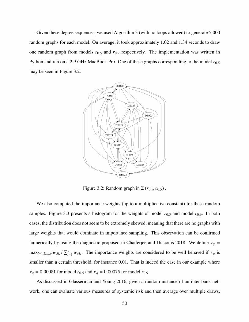
Given these degree sequences, we used Algorithm 3 (with no loops allowed) to generate 5,000
random graphs for each model. On average, it took approximately 1.02 and 1.34 seconds to draw
one random graph from models r0.5 and r0.9 respectively. The implementation was written in
Python and ran on a 2.9 GHz MacBook Pro. One of these graphs corresponding to the model r0.5
may be seen in Figure 3.2.
DE020
DE019
DE021
DE022
DE017
DE024
DE023
DE018
DE028
DE027
DE025
Figure 3.2: Random graph in Σ (r0.5, c0.5) .
We also computed the importance weights (up to a multiplicative constant) for these random
samples. Figure 3.3 presents a histogram for the weights of model r0.5 and model r0.9. In both
cases, the distribution does not seem to be extremely skewed, meaning that there are no graphs with
large weights that would dominate in importance sampling. This observation can be confirmed
numerically by using the diagnostic proposed in Chatterjee and Diaconis 2018. We define κq =
maxi=1,2,...,q wMi/∑q
i=1 wMi . The importance weights are considered to be well behaved if κq is
smaller than a certain threshold, for instance 0.01. That is indeed the case in our example where
κq = 0.00081 for model r0.5 and κq = 0.00075 for model r0.9.
As discussed in Glasserman and Young 2016, given a random instance of an inter-bank net-
work, one can evaluate various measures of systemic risk and then average over multiple draws.
50
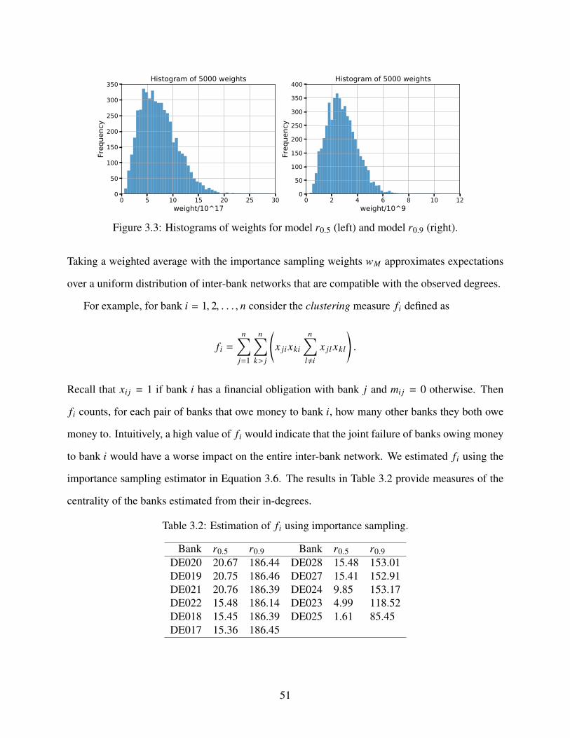
0 5 10 15 20 25 30weight/10^17
0
50
100
150
200
250
300
350
Freq
uenc
y
Histogram of 5000 weights
0 2 4 6 8 10 12weight/10^9
0
50
100
150
200
250
300
350
400
Freq
uenc
y
Histogram of 5000 weights
Figure 3.3: Histograms of weights for model r0.5 (left) and model r0.9 (right).
Taking a weighted average with the importance sampling weights wM approximates expectations
over a uniform distribution of inter-bank networks that are compatible with the observed degrees.
For example, for bank i = 1, 2, . . . , n consider the clustering measure fi defined as
fi =
n∑j=1
n∑k> j
*,
x ji xki
n∑l,i
x jl xkl+-.
Recall that xi j = 1 if bank i has a financial obligation with bank j and mi j = 0 otherwise. Then
fi counts, for each pair of banks that owe money to bank i, how many other banks they both owe
money to. Intuitively, a high value of fi would indicate that the joint failure of banks owing money
to bank i would have a worse impact on the entire inter-bank network. We estimated fi using the
importance sampling estimator in Equation 3.6. The results in Table 3.2 provide measures of the
centrality of the banks estimated from their in-degrees.
Table 3.2: Estimation of fi using importance sampling.
Bank r0.5 r0.9 Bank r0.5 r0.9DE020 20.67 186.44 DE028 15.48 153.01DE019 20.75 186.46 DE027 15.41 152.91DE021 20.76 186.39 DE024 9.85 153.17DE022 15.48 186.14 DE023 4.99 118.52DE018 15.45 186.39 DE025 1.61 85.45DE017 15.36 186.45
51

3.5 Further Numerical Experiments for the Graph Case
Recall that Algorithm 1 simulates each point x ∈ Sh sequentially, that is, component by com-
ponent. The order in which the entries are selected can be determined by the user and, in principle,
can be a fixed, adaptive, or even a random order. Regardless of the order rule, Algorithm 1 will
always run to completion and return a valid point in the target set. However, as discussed in Sec-
tion 2.5.4, the order rule can affect the distribution of the importance sampling weights. If we are
interested in computing estimates using importance sampling, we should prefer order rules that
make the weights distribution as uniform as possible — that is, without the outliers of a highly
skewed distribution. The main objective of this section is to assess the effect that different adaptive
order rules have on the importance sampling weights, when sampling random graphs (in the binary
case) using Algorithm 1. We compare the following four order rules:
• Fixed order (F). Entries are selected in order from 1 to n.
• Random order (RN). Entries are selected uniformly at random from the set of remaining
entries.
• Most uniform adaptive order (MU). This is the rule introduced in Definition 1. Entries are
selected by selecting the entry i that has the most uniform marginal distribution. That is, the
one with natural parameter ηi closest to zero.
• Most singular adaptive order (MS). In a sense, this rule is opposite to MU. Entries are se-
lected by selecting the entry i that has the marginal distribution closest to a point mass at
either zero or one. That is, the one with largest natural parameter ηi in absolute value.
We test these order rules on three directed and one undirected graph degree sequences:
• Interbank-1: r = c = (6, 6, 6, 5, 5, 5, 5, 4, 4, 3, 2),
• Interbank-2: r = c = (9, 9, 9, 9, 9, 9, 8, 8, 8, 7, 6),
52
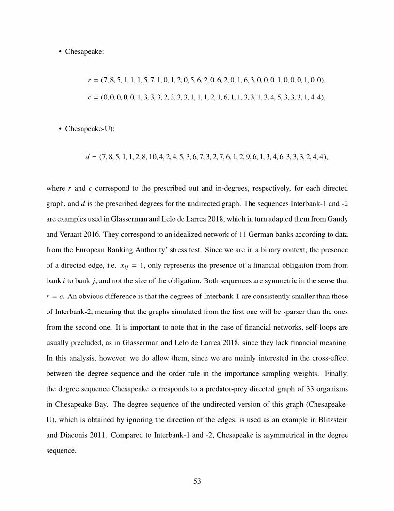
• Chesapeake:
r = (7, 8, 5, 1, 1, 1, 5, 7, 1, 0, 1, 2, 0, 5, 6, 2, 0, 6, 2, 0, 1, 6, 3, 0, 0, 0, 1, 0, 0, 0, 1, 0, 0),
c = (0, 0, 0, 0, 0, 1, 3, 3, 3, 2, 3, 3, 3, 1, 1, 1, 2, 1, 6, 1, 1, 3, 3, 1, 3, 4, 5, 3, 3, 3, 1, 4, 4),
• Chesapeake-U):
d = (7, 8, 5, 1, 1, 2, 8, 10, 4, 2, 4, 5, 3, 6, 7, 3, 2, 7, 6, 1, 2, 9, 6, 1, 3, 4, 6, 3, 3, 3, 2, 4, 4),
where r and c correspond to the prescribed out and in-degrees, respectively, for each directed
graph, and d is the prescribed degrees for the undirected graph. The sequences Interbank-1 and -2
are examples used in Glasserman and Lelo de Larrea 2018, which in turn adapted them from Gandy
and Veraart 2016. They correspond to an idealized network of 11 German banks according to data
from the European Banking Authority’ stress test. Since we are in a binary context, the presence
of a directed edge, i.e. xi j = 1, only represents the presence of a financial obligation from from
bank i to bank j, and not the size of the obligation. Both sequences are symmetric in the sense that
r = c. An obvious difference is that the degrees of Interbank-1 are consistently smaller than those
of Interbank-2, meaning that the graphs simulated from the first one will be sparser than the ones
from the second one. It is important to note that in the case of financial networks, self-loops are
usually precluded, as in Glasserman and Lelo de Larrea 2018, since they lack financial meaning.
In this analysis, however, we do allow them, since we are mainly interested in the cross-effect
between the degree sequence and the order rule in the importance sampling weights. Finally,
the degree sequence Chesapeake corresponds to a predator-prey directed graph of 33 organisms
in Chesapeake Bay. The degree sequence of the undirected version of this graph (Chesapeake-
U), which is obtained by ignoring the direction of the edges, is used as an example in Blitzstein
and Diaconis 2011. Compared to Interbank-1 and -2, Chesapeake is asymmetrical in the degree
sequence.
53
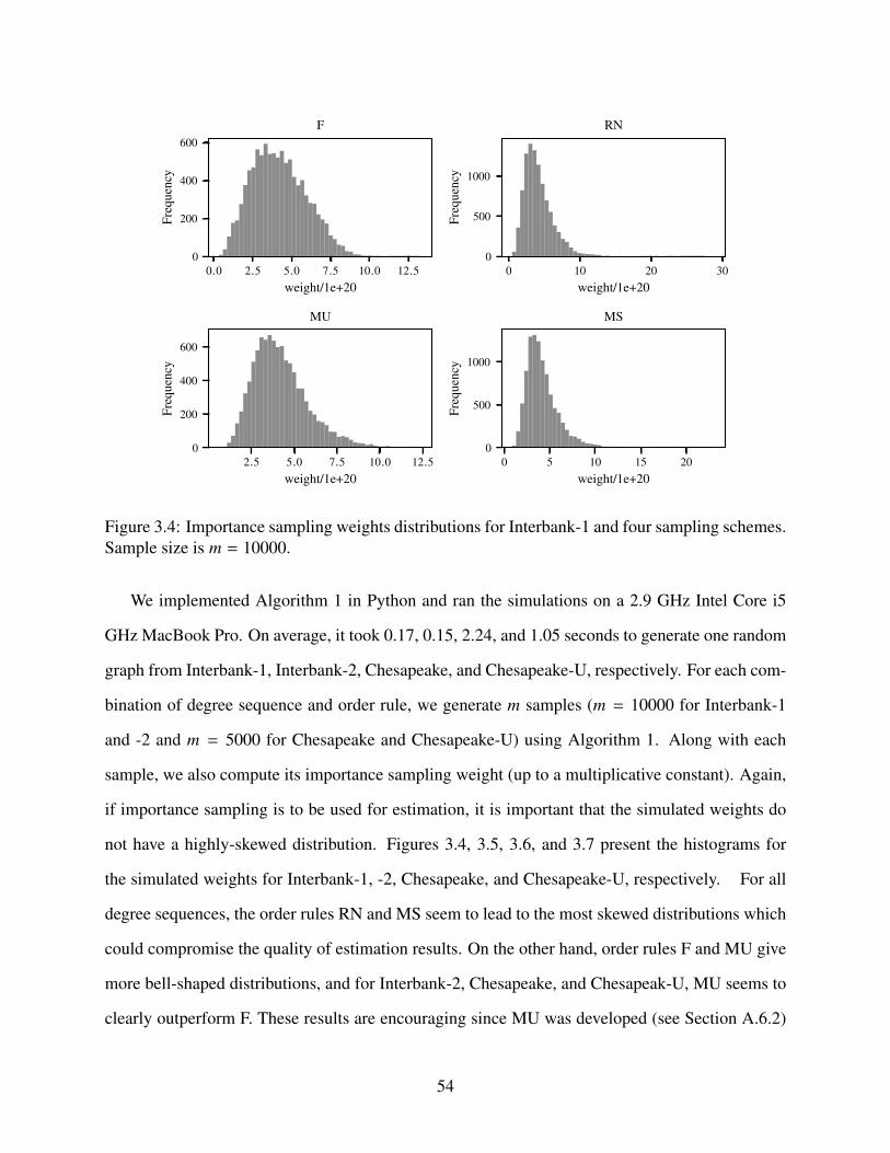
0.0 2.5 5.0 7.5 10.0 12.5weight/1e+20
0
200
400
600
Freq
uenc
y
F
0 10 20 30weight/1e+20
0
500
1000
Freq
uenc
y
RN
2.5 5.0 7.5 10.0 12.5weight/1e+20
0
200
400
600
Freq
uenc
y
MU
0 5 10 15 20weight/1e+20
0
500
1000
Freq
uenc
y
MS
Figure 3.4: Importance sampling weights distributions for Interbank-1 and four sampling schemes.Sample size is m = 10000.
We implemented Algorithm 1 in Python and ran the simulations on a 2.9 GHz Intel Core i5
GHz MacBook Pro. On average, it took 0.17, 0.15, 2.24, and 1.05 seconds to generate one random
graph from Interbank-1, Interbank-2, Chesapeake, and Chesapeake-U, respectively. For each com-
bination of degree sequence and order rule, we generate m samples (m = 10000 for Interbank-1
and -2 and m = 5000 for Chesapeake and Chesapeake-U) using Algorithm 1. Along with each
sample, we also compute its importance sampling weight (up to a multiplicative constant). Again,
if importance sampling is to be used for estimation, it is important that the simulated weights do
not have a highly-skewed distribution. Figures 3.4, 3.5, 3.6, and 3.7 present the histograms for
the simulated weights for Interbank-1, -2, Chesapeake, and Chesapeake-U, respectively. For all
degree sequences, the order rules RN and MS seem to lead to the most skewed distributions which
could compromise the quality of estimation results. On the other hand, order rules F and MU give
more bell-shaped distributions, and for Interbank-2, Chesapeake, and Chesapeak-U, MU seems to
clearly outperform F. These results are encouraging since MU was developed (see Section A.6.2)
54
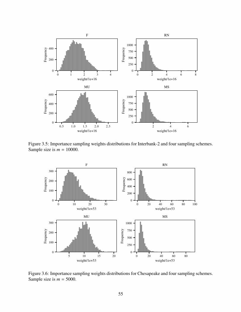
0 1 2 3 4weight/1e+16
0
200
400Fr
eque
ncy
F
0 2 4 6 8weight/1e+16
0
250
500
750
1000
Freq
uenc
y
RN
0.5 1.0 1.5 2.0 2.5weight/1e+16
0
200
400
600
Freq
uenc
y
MU
2 4 6weight/1e+16
0
250
500
750
1000
Freq
uenc
y
MS
Figure 3.5: Importance sampling weights distributions for Interbank-2 and four sampling schemes.Sample size is m = 10000.
0 10 20 30weight/1e+53
0
100
200
300
Freq
uenc
y
F
0 20 40 60 80 100weight/1e+53
0
200
400
600
800
Freq
uenc
y
RN
5 10 15 20weight/1e+53
0
100
200
300
Freq
uenc
y
MU
0 20 40 60 80weight/1e+53
0
250
500
750
1000
Freq
uenc
y
MS
Figure 3.6: Importance sampling weights distributions for Chesapeake and four sampling schemes.Sample size is m = 5000.
55

0 1 2 3 4weight/1e+57
0
100
200Fr
eque
ncy
F
0 5 10 15weight/1e+57
0
200
400
600
800
Freq
uenc
y
RN
0 1 2 3weight/1e+57
0
100
200
300
400
Freq
uenc
y
MU
0 5 10 15weight/1e+57
0
500
1000
Freq
uenc
y
MS
Figure 3.7: Importance sampling weights distributions for Chesapeake-U and four samplingschemes. Sample size is m = 5000.
as a heuristic to address the loss of uniformity of Algorithm 1.
Besides the visual inspections of the simulated weights distributions, we use two quantita-
tive diagnostics to assess the quality of the importance sampling weights. Given weights w =
(w1, . . . ,wm), we define D1(w) , max {wi} /median {wi} , D2(w) , max {wi} /(∑m
j=1 w j ). Diag-
nostic D1 is used in Blitzstein and Diaconis 2011, and D2 proposed in Chatterjee and Diaconis
2018. The weights are considered well-behaved if either D1 or D2 are smaller than a certain arbi-
trary threshold, for instance, 0.01 for D2. We compute D1 and D2 and report the results in Table
3.3. Observe that for all cases, D1 and D2 seem to be small. All the values of D2 are lower
than the threshold of 0.01, and for comparison, Blitzstein and Diaconis 2011 report D1 = 52 for
Chesapeake-U using their simulation algorithm. This speaks to the quality of the importance sam-
pling weights using Algorithm 1. Furthermore, note that for all combinations of degree sequence
and diagnostic, the minimum value is attained by the MU order rule. This corroborates our initial
visual observation that MU seems to indeed improve the uniformity of the weights compared to
56

Table 3.3: Quality diagnostics for the simulated importance sampling weights. D1 and D2 arecomputed for each combination of degree sequence and order rule.
D1 D2
F RN MU MS F RN MU MS
Interbank-1 3.3 7.7 3.1 6.1 3.2e-04 6.9e-04 3.0e-04 5.5e-04Interbank-2 3.1 6.0 2.0 5.3 3.1e-04 5.6e-04 2.0e-04 4.8e-04Chesapeake 4.0 12.2 2.1 11.1 7.4e-04 2.0e-03 4.2e-04 1.9e-03Chesapeake-U 3.1 12.6 2.1 12.8 5.9e-04 2.1e-03 4.3e-04 2.3e-03
other rules.
57

Chapter 4: New York City Hospital Load Balancing
4.1 The Simulation Model
The simulation model is a computational program which represents the main objects, agents,
and dynamics of an EMS system. Although this model is tailored to the structure, operations, and
needs of NYC’s EMS system, it can be modified accordingly to other cities or geographies. The
code is written in Python, which allows for user-friendly visualizations.
4.1.1 New York City Geography
For EMS operations, the FDNY divides NYC into nearly 2,400 geographical areas (polygons),
also known as atoms. Certain decisions, such as ambulance dispatch to an incident or hospital
selection for a transport, are made at the atom level. For instance, two incidents in the same atom,
that require a hospital transport with the same (critical) care category, will usually be assigned to
the same hospital. Given the relevance of atoms in the EMS system, the simulation model reads
the atom geographical information (boundaries, and a user-defined centroid) from an external file.
All the virtual objects of the model will be located within the boundaries established by this file
(with the exception of some EMS hospitals which are located outside NYC proper).
4.1.2 EMS Objects
The simulation model is built using the discrete event simulation methodology and has an
object-oriented structure. We define several classes representing real-life EMS objects. The ob-
jects’ attributes can be read by the model from external files. The following is a brief description
of the main objects of the model.
Ambulances: also called units (we use either term indistinguishably from now on). There are
58

two types of ambulances: basic life support (BLS) and advanced life support (ALS). BLS units
treat low acuity incidents, while ALS units are designated to high acuity ones. For the most critical
incidents, two ambulances (one BLS and one ALS) will be dispatched to the scene. Ambulances
work in schedules (also known as tours) which are either 8 or 12 hours long. Each unit has an
assigned standby position, known as the cross-street location (CSL). Between incident responses,
the ambulance remains at its CSL, waiting for the next incident. Once the tour ends, the ambulance
goes back to its assigned station, where a crew shift occurs and a new tour begins. Finally, the EMS
system includes both ambulances managed either directly by the FDNY (municipal units) or by the
hospitals (voluntary units). Both municipal and voluntary units are coordinated for dispatch and
hospital transport through NYC’s 911 system via the EMS dispatch system. The model contains
the information and CSL of around 500 units distributed across the city.
Hospitals: In general, hospitals receive patients via walk-in, inter-facility transport, and 911
transport. In this model however, we only keep track of 911 transports, which are the ones directly
related to EMS operations. Each hospital has a different capacity level which evolves through
time. On one hand, new patient transports arrive to the hospital, a percentage of which (currently
set to 40%) will occupy a bed, thus reducing the hospital capacity. On the other hand, we assume
a random hospital discharge process which simulates patient discharges, increasing the hospital
capacity. See Section 4.1.4 for more details on the discharge process. Even when the hospital is at
zero capacity, the model allows for new patients to be transported to it. In that case, the hospital
becomes overloaded and the hospital’s bed occupancy surpasses 100%. This behavior is reflective
of real-life situations (see Figure 1.1). Additionally, not all hospitals have the resources to accept
all patient types. For instance, not all hospitals are equipped to treat severe burns or stroke patients.
All 911 receiving hospitals in NYC do accept General Emergency Department patients. The model
contains the information of more than 60 hospitals that are part of the EMS system (not all of them
in NYC proper).
Ambulance Stations: These buildings house FDNY ambulances when they are out of service or
between tours. Municipal units are assigned to an ambulance station, whereas voluntary units use
59

their hospital as base. The model contains the information of 40 ambulance stations.
Incidents: After a medical incident is reported to the 911 system, unit(s) will be dispatched
based on the location and severity of the incident. Upon arrival, the crew spends time on-scene
tending to and evaluating the patient. If the patient needs to go to a hospital, the unit will proceed
with the transport. The incident’s acuity or severity is assessed in two stages. An initial sever-
ity level (coded as 1–8), which in practice is selected by a medically trained call taker utilizing
computerized triage, determines the resource type (BLS or ALS) and number of units that are dis-
patched. Once at the scene, the EMS crew will reassess the situation and, if a hospital transort is
necessary, assign a care category to the patient. The atom location and care category enable the
EMS dispatch system to provide a list of recommended hospitals in order of closest to furthest
from the incident location. The model allows for the use of either historical or random incidents.
Feeding historical incidents into the model is particularly useful when the user wishes to “replay”
certain periods of time, while changing certain policies or model inputs. See Section 4.1.4 for
more details on how to simulate random incidents.
Dispatcher: This object represents a fictional “main” agent who acts as the system decision
maker. The dispatcher decides which unit(s) will be dispatched to an incoming incident and, if a
transport is required, to which hospital the patient will be sent. In real life, the role of the dispatcher
is a joint effort between human dispatchers, the EMS dispatch system, and a set of policies.
EMS System: a parent object that contains all of the other EMS objects. It defines a simulation
window, sets up an initial configuration for the objects, and starts the simulation clock. During a
simulation run, it also gathers several metrics and statistics for posterior analysis.
4.1.3 Model Dynamics
The main dynamics of the model are standard and similar across different EMS systems; see
Figure 4.1. We summarize them as follows:
1. Incident arrival: A new incident is generated and its location and severity level are informed
to the dispatcher.
60

2. Unit assignment (dispatch): According to the incident characteristics, the dispatcher assigns
one or more ambulances to it. As a general rule, low acuity incidents (severity levels 4–8)
get assigned to one BLS unit, higher acuity incidents (severity levels 2–3) get assigned to
one ALS unit, and the most severe incidents (severity level 1) get assigned to two units (one
of each). The dispatcher selects the necessary units according to shortest estimated time of
arrival. If no units are available, the incident is pushed into a waiting queue.
3. On-scene treatment: Once the unit arrives to the incident location, the care category of the
patient is determined. If the patient does not require to be transported to a hospital, then the
unit finishes the job and returns to its CSL.
4. Hospital assignment: If the patient needs to go to a hospital, the dispatcher will proceed to
assign an appropriate hospital. The default behavior is to follow the closest hospital rule.
This is the hospital with the necessary equipment to treat the incident’s care category and
with shortest estimated time of arrival from the atom location. For an alternative to the
closest hospital rule, we define in Section 4.3 a load balancing rule that takes into account
the citywide hospital capacities.
5. At-hospital procedure: Once the ambulance arrives to the hospital, it delivers the patient and
finishes the current job. It travels back to its CSL and becomes available for a new incident
assignment (if required, it can be assigned to a new job before reaching the CSL). The patient
(with some probability) gets admitted and occupies a bed (effectively lowering the hospital
bed capacity by one). Some (random) time later, the patient is discharged and the hospital
bed capacity increases by one.
4.1.4 Sub-models
Besides the main dynamics discussed above, the simulation system requires additional sub-
models that will inject the “randomness” into the model. These models address dynamics that are,
in their own right, interesting and complex. In this paper, we often opt to use simple models, but
61
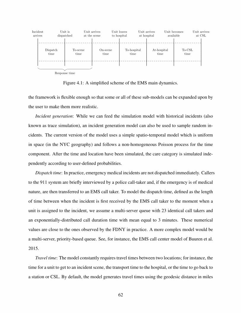
Dispatchtime
To-scenetime
On-scenetime
To-hospitaltime
At-hospitaltime
To-CSLtime
Incidentarrives
Unit isdispatched
Unit arrivesat the scene
Unit leavesto hospital
Unit arrivesat hospital
Unit becomesavailable
Unit arrivesat CSL
Response time
Figure 4.1: A simplified scheme of the EMS main dynamics.
the framework is flexible enough so that some or all of these sub-models can be expanded upon by
the user to make them more realistic.
Incident generation: While we can feed the simulation model with historical incidents (also
known as trace simulation), an incident generation model can also be used to sample random in-
cidents. The current version of the model uses a simple spatio-temporal model which is uniform
in space (in the NYC geography) and follows a non-homogeneous Poisson process for the time
component. After the time and location have been simulated, the care category is simulated inde-
pendently according to user-defined probabilities.
Dispatch time: In practice, emergency medical incidents are not dispatched immediately. Callers
to the 911 system are briefly interviewed by a police call-taker and, if the emergency is of medical
nature, are then transferred to an EMS call taker. To model the dispatch time, defined as the length
of time between when the incident is first received by the EMS call taker to the moment when a
unit is assigned to the incident, we assume a multi-server queue with 23 identical call takers and
an exponentially-distributed call duration time with mean equal to 3 minutes. These numerical
values are close to the ones observed by the FDNY in practice. A more complex model would be
a multi-server, priority-based queue. See, for instance, the EMS call center model of Buuren et al.
2015.
Travel time: The model constantly requires travel times between two locations; for instance, the
time for a unit to get to an incident scene, the transport time to the hospital, or the time to go back to
a station or CSL. By default, the model generates travel times using the geodesic distance in miles
62

between two locations and by assuming a constant ambulance speed. This simple approach has
been used before Silva and Pinto 2010. We assume that the speed is higher when the unit is on a job
(i.e. going to a scene or transporting patients to a hospital). In addition, for travel times between
incident locations and hospitals, the model can use an external travel time matrix. If this matrix is
properly calibrated with ambulance traffic data, it can improve the fidelity of the simulation model.
An important difference between these two approaches is the granularity: geodesic distances can
be computed between any two pairs of latitude-longitude coordinates, whereas the travel time
matrix uses the incident and hospital atoms as input.
On-scene time: The time that an EMS crew takes to treat the patient can depend on the severity
level and care category, among other factors. We currently assume a uniform distribution.
At-hospital time: Once the ambulance arrives to the hospital, it has to wait some time while
the hospital personnel admits the patient into the emergency department. This time most likely
depends on the saturation level of the hospital. We currently assume a uniform distribution.
Hospital patient discharge: Modeling the hospital-side of an EMS system is particularly chal-
lenging, especially from the standpoint of the EMS system manager. Whereas EMS managers
have access to data from their dispatchers and ambulances, having precise and frequent feedback
from the hospitals is not always a reality. In our setting, we are interested in modeling the rate at
which hospitals discharge patients, effectively increasing their capacity. We do so by considering
an initial estimated capacity level and a pure-death process for the discharge times. We calibrate
this model to achieve a long-term “equilibrium” of hospital occupancy during periods where the
number of incidents and hospital transports are relatively stable. See Appendix C.1 for more details
on the calibration of this model.
Out of service: Ambulances can go out of service for a variety of reasons (such as unit main-
tenance, staffing issues or mechanical failures). This will partially or totally interrupt a scheduled
tour, reducing ambulance availability. We assume that units can randomly go out of service, with
a certain probability, only after finishing a hospital transport.
63

4.2 Load Balancing Optimization Problem
Given an EMS system with m atoms and n hospitals, our objective is to assign one hospital
to each atom by minimizing the total (estimated) travel time subject to the hospital capacity con-
straints. The decision variables can be seen as indicators xi j ∈ {0, 1}, where xi j = 1 if and only if
hospital j is assigned to atom i.
At the beginning of each simulated day, we gather the following inputs:
• The predicted daily hospital transports originating from atom i for the next day, denoted as
fi ∈ Z+. In this application, we naively estimate fi as the running average of transports of
the last d = 3 days.
• The current bed availability at hospital j ∈ {1, . . . , n}, denoted as c j ∈ Z. A negative c j
indicates that the hospital is overwhelmed and that it currently has −c j > 0 patients above
its total capacity.
• The estimated time of arrival from atom i to hospital j, denoted as Ti j ∈ R+.
• The expected proportion of transported patients that are admitted to the hospital, denoted as
δ ∈ (0, 1). We currently use δ = 0.4.
With these inputs, we solve the following integer optimization problem to update the hospital
assignment rule:
minimizex
m∑i=1
n∑j=1
fiTi j xi j
subject tom∑
i=1
δ fi xi j ≤ max(c j, 0), for all j,
n∑j=1
xi j = 1, for all i,
xi j ∈ {0, 1}, for all i, j .
Extensions to this optimization problem are presented in Appendix C.2.
64

4.3 Hospital Load Balancing Application
We test our simulation model in the context of a new hospital load balancing rule. The standard
rule for hospital assignment sends the patient to the closest appropriate hospital. Intuitively, this
rule makes sense because the patient is provided with fast medical care and the ambulance is able
to finish the current job and report back for duty as soon as possible. This approach, however, does
not take into account the capacity level of hospitals.
In the presence of critical external events, such as natural disasters or pandemics, the number
of patient transports to a hospital might increase drastically. This could lead to the hospital being
overloaded which in turn could compromise patient care. To avoid this scenario, we propose a new
hospital assignment rule which attempts to achieve load balancing across the hospital system.
The standard closest hospital rule can be summarized by a function that maps each atom to
its closest hospital. The output of the load balancing rule is another function, which still assigns
hospitals to atoms, but does so by considering both (a) the distance between atom and hospital and
(b) the hospital capacity. The procedure to determine the load balancing function is to solve an
integer optimization problem which minimizes the system-wide hospital transport time subject to
hospital capacity constraints. See Appendix 4.2 for the mathematical formulation of this problem
and the details of its inputs.
Solving the load balancing problem requires as an input, among others, an estimate of the daily
bed capacity levels of each hospital in the system. In real life, the FDNY has access to daily
updates on these values, so we can run the load balancing optimization and update the hospital
assignment function each day (the availability and frequency of this data might be different for
other cities).
4.3.1 Simulation Setup
We now conduct a simulation study to assess the impact of implementing the load balancing
rule on the EMS system. The simulation setup is as follows. We select a simulation window of
65

14 days. Since we have access to real-life incident data, we feed into the model all the incidents
received from March 25th, 2020 and April 7th, 2021. This period corresponds to some of the
weeks with highest incident counts during the COVID-19 epidemic in NYC. For reference, during
this period, the system received on average more than 5,500 incidents per day. In contrast, during
regular times, this quantity hovers around 4,000. For simplicity, we assume that all incidents
requiring a transport had a General Emergency Department care category. In reality, this care
category amounts to around 80% of total transports.
When computing travel times, we differentiate between hospital transport times and other travel
times. To increase accuracy, for hospital transport times we use a travel time matrix calibrated with
historical ambulance data and network analysis. For the rest of the travel times, we use the geodesic
model with constant speed of 12 miles per hour for units on a job and 9 miles per hour for off-duty
units.
To simulate the evolution of the hospitals’ capacity levels, we first assume a city-wide hos-
pital occupancy level of 80%. The total number of beds per hospital is estimated using publicly
available data from the New York State Department of Health. The patient discharge process is
then calibrated using the procedure described in Appendix C.1. We assume that in a normal day,
there are approximately 2,900 hospital transports (this is assuming an estimated 1.5 million yearly
incidents, 70% of which result in a transport).
4.3.2 Hospital Assignment Rule Comparison
We run two simulations using the same setup described in the previous section. The difference
between them is the hospital assignment rule that is assumed. The first simulation uses the closest-
hospital rule. The second one uses the load balancing rule, where the hospital assignment per atom
is updated at the beginning of each simulated day.
Several metrics are of interest when evaluating these rules. The first one is the hospital oc-
cupancy level as a function of time. The load balancing rule should keep these levels in check,
since it is designed to deviate transports to hospitals which are not saturated. Figure 4.2 presents
66

a side-by-side comparison of both rules, for one simulation run. When the closest hospital rule
is followed (left panel of Figure 4.2), several hospitals reach their maximum capacity level and
become overloaded. This occurs to hospitals that are close to a high number of incidents and do
not have the capacity to meet the demand. In contrast, when the load balancing rule is in place, the
transports to hospitals are better distributed (right panel of Figure 4.2). In this scenario there are
still hospitals that might reach their maximum capacity levels and might even briefly surpass them.
This is due to the randomness of the hospital discharge model and the fact that our incident predic-
tion for the next day is not exact (see Appendix 4.2). Even with these factors into consideration,
the load balancing rule is able to correctly keep hospital capacity overloads in check.
The simulated values in Figure 4.2 are for illustration purposes only and should not be taken
as reflective of a real-life situation. In particular, we note that such high occupancy levels would
be prevented in real-time via hospital redirection, diversion, and internal load balancing policies.
A redirection occurs when the EMS dispatch system detects that a certain hospital shows signs
of overloading. For instance, a redirection might be triggered when a certain number of units
spend too long stationed in the hospital’s emergency department. Similarly, a hospital staff might
request a hospital diversion directly to the EMS system, if they consider they are temporarily
unable to receive more patients. Finally, a hospital is capable of load balancing itself via inter-
facility transports. In this simulation scenario, we do not consider such real-time policies. That
being said, in practice, load balancing would work jointly with the other policies to better load
balance the hospital system.
Recall that, with the load balancing rule, there is a trade-off between hospital transport time
and hospital capacities. Indeed, if ambulances are dispatched to hospitals with capacity, that may
not be the closest ones, the overall transport times will inevitably increase. In addition, sending
units to farther away hospitals may have an indirect impact on the average incident response time
(defined as the time between the incident arrival and the unit arrival at the scene; see Figure 4.1).
If the ambulances are transporting patients away from their usual area, they might not be able to
respond as fast to new incidents. We explore the impact of imposing the load balancing rule on
67

0 50 100 150 200 250 300 350Simulated time (hours)
50
100
150
200
250
300
Hosp
ital b
ed o
ccup
ancy
(%)
Closest Hospital
0 50 100 150 200 250 300 350Simulated time (hours)
Load Balancing
Figure 4.2: Comparison of the simulated hospital capacities using both hospital assignment rules:closest hospital (left) and load balancing (right). Each line corresponds to the proportion of occu-pied beds of a NYC hospital. The dashed gray line corresponds to a 100% occupancy level. Thedata is illustrative only.
both metrics (hospital transport and response times) in Table 4.1. The statistics presented are based
on one simulation run for each rule.
In this simulation, the average transport time increases by 1.6 minutes, when we use the load
balancing rule. This increase is by no means negligible, but for low acuity patients, it should not
be life-threatening. We do see a deterioration in the tail of the distribution; the 99th percentile
increases considerably from 17.8 to 23.4 minutes. This reinforces the belief that load balancing
should only be used for non-critical transports. If an upper bound on the admissible transport times
is required (say, for instance 30 or 40 minutes), it can be imposed by modifying the load balanc-
ing optimization problem. On the other hand, ambulance response times were not so adversely
affected by the load balancing rule. The mean response time increased by less than half a minute
and, although the response times do tend to be larger, the 99th percentile only increased in 0.3
minutes. It should be noted that the underlying travel time model used to compute response times
is too simplistic (it is based on the geodesic distance and a constant unit speed), and therefore, the
numerical results might not reflect the reality. In this study, however, we are more interested in the
68

Table 4.1: Summary statistics for the hospital transport and unit response times. All the times arein minutes.
Hospital Transport Time Response TimeClosest Hospital Load Balancing Closest Hospital Load Balancing
mean 9.2 10.8 6.6 6.7std 3.0 4.4 4.6 4.7median 8.9 9.9 5.5 5.695-percentile 14.3 19.1 15.0 15.499-percentile 17.8 23.4 21.9 22.2
difference in the shapes of the distributions and not so much in particular numerical values.
4.3.3 Main Limitations
The main limitation of the simulation model comes from the simplifying assumptions made on
the hospital patient arrival and discharge processes. While they are only part of our entire model,
these processes are incredibly complex and deserve their own individual studies. Another limi-
tation comes from the simple geodesic travel time model. We corrected the travel times between
locations and hospitals using an external matrix that was calibrated with ambulance traffic data and
network analysis, but we did not make the extension to general travel times between two arbitrary
locations. Finally, we opted for simple sub-models for dispatch, on-scene, and at-hospital times.
The primary objective of using the simulation model to assess the new load balancing rule was
to check the high-level dynamics and detect any potential issues. Due to the urgency of real-life
implementation, we have not presented a formal validation of the model. To do the latter task, we
first would need to refine all the sub-models mentioned above and calibrate them using real data.
All these improvements are important ongoing work.
69
Chapter 5: Conclusions
In this thesis, we have showcased the utility of simulation techniques when approaching chal-
lenging problems. In particular, simulation is useful to study both theoretical problems, such as
sampling graphs with prescribed degree sequences, and practical problems, such as analyzing the
performance of a real-life emergency medical services system.
5.1 Concluding Remarks for Part 1
We have addressed the problem of sampling uniformly from product sets subject to linear con-
straints, which has, as an important particular case, the problem of sampling bipartite (weighted)
graphs with prescribed degree sequences. We defined a maximum entropy distribution which sam-
ples uniformly conditional on sampling from the target set. We showed that this distribution is the
max-min probability distribution if and only if its mean lies in the convex hull of the target set.
We proposed a sequential algorithm that relies mainly on the sequential computation of the
maximum entropy distribution. This algorithm can be used, in particular, to generate random
bipartite or directed graphs with a determined degree sequence. In this case, the entries of the
maximum entropy matrix determine the individual edge probabilities that the algorithm uses. We
showed that the algorithm always samples from the target set and generates each feasible point
with positive probability, although the outcomes will not be distributed uniformly. For estimation
under the uniform distribution, we applied importance sampling weights given by the sequential
algorithm. The application to an inter-bank network produced weights with a reasonable distri-
bution, that is, not extremely skewed. We argued that using a most-uniform adaptive order rule
should improve the quality of the importance sampling weights and provided evidence through
numerical experiments.
70
In the general case, the sequential algorithm requires checking the feasibility of subproblems
at each step. We showed that feasibility is automatic in the binary case (like in the graph case)
and tractable to verify with totally unimodular constraints. We leave the question of whether
feasibility can be checked efficiently in other cases for future work. Another research direction
lies towards developing an update rule for the maximum entropy distribution. The computation
of this distribution is the most computationally expensive operation of the sequential algorithm,
since it involves solving a convex optimization problem. Therefore, finding a way to quickly
update P∗ (even approximately) using its value in the previous iteration could potentially lead to
a considerable speed-up in runtime. Finally, expanding our methodology to nonlinear constraints,
an important feature for social network analysis, is also left for future research.
5.2 Concluding Remarks for Part 2
The FDNY requires analytical tools to better understand the impact of potential policy changes
to their EMS system. To this goal, we implemented an EMS simulation model for NYC. The
model captures the main objects and dynamics of the system. Like similar models in the literature,
our model can use trace simulation (i.e. using historical data) for the incident arrival process. This
allows the user to test several scenarios and changes in policy, subject to incidents observed in the
past.
We used the simulation model to evaluate a new hospital load balancing approach, which differs
from the standard and widely-used rule of sending patients to the closest hospital. This approach
minimizes the overall patient transport time, but also takes into account the capacity levels of the
hospitals. Assuming a particular patient discharge model, we showed in our simulation that the
load balancing rule effectively keeps the individual hospital occupancy rates below the at-capacity
level. In contrast, using load balancing would result in longer transport times (unit response times
were not so clearly affected). This observation suggests that load balancing might be beneficial for
the EMS system as a whole, but it should only be used for patients that are not high acuity.
Simulation is an essential tool when considering the impact of a new policy, especially in criti-
71

cal areas such as EMS. It helps decision makers to quantify and visualize several scenarios, before
making changes in real life. Our analysis assisted in the FDNY’s decision to implement the load
balancing rule in response to the COVID-19 pandemic. The new rule works in addition to preex-
isting hospital redirection and diversion policies and will hopefully serve as an extra safeguard for
balancing system-wide hospital capacity levels.
72
References
Aboueljinane, L., E. Sahin, and Z. Jemai (2013). “A review on simulation models applied to emer-gency medical service operations”. In: Computers & Industrial Engineering 66.4, pp. 734–750.
Aboueljinane, L., E. Sahin, Z. Jemai, and J. Marty (2014). “A simulation study to improve theperformance of an emergency medical service: Application to the French Val-de-Marne de-partment”. In: Simulation Modelling Practice and Theory 47, pp. 46–59.
Ahn, D. and K.-K. Kim (2018). “Efficient simulation for expectations over the union of half-spaces”. In: ACM Transactions on Modeling and Computer Simulation (TOMACS) 28.3, p. 23.
Anand, K., I. van Lelyveld, Á. Banai, S. Friedrich, R. Garratt, G. Hałaj, J. Fique, I. Hansen, S.Martínez Jaramillo, H. Lee, J. L. Molina-Borboa, S. Nobili, S. Rajan, D. Salakhova, T. C.Silva, L. Silvestri, and S. R. Stancato de Souza (2018). “The Missing Links: A Global Study onUncovering Financial Network Structures from Partial Data”. In: Journal of Financial Stability35, pp. 107–119.
Aringhieri, R., S. Bocca, L. Casciaro, and D. Duma (2018). “A Simulation and Online Optimiza-tion Approach for the Real-Time Management of Ambulances”. In: Proceedings of the 2018Winter Simulation Conference. Ed. by M. Rabe, A. A. Juan, N. Mustafee, A. Skoogh, S. Jain,and B. Johansson. Piscataway, New Jersey: Institute of Electrical and Electronics Engineers,Inc., pp. 2554–2565.
Avellaneda, M., R. Buff, C. Friedman, N. Grandchamp, L. Kruk, and J. Newman (2000). “WeightedMonte Carlo: A new technique for calibrating asset-pricing models”. In: Applied and IndustrialMathematics, Venice—2, 1998. Ed. by R. Spigler. Springer, pp. 1–31.
Barvinok, A. (2010). “On the number of matrices and a random matrix with prescribed row andcolumn sums and 0–1 entries”. In: Advances in Mathematics 224.1, pp. 316–339.
Bertsimas, D. and J. N. Tsitsiklis (1997). Introduction to Linear Optimization. Athena Scientific.
Blanchet, J. H. (2009). “Efficient importance sampling for binary contingency tables”. In: TheAnnals of Applied Probability 19.3, pp. 949–982.
Blitzstein, J. and P. Diaconis (2011). “A sequential importance sampling algorithm for generatingrandom graphs with prescribed degrees”. In: Internet mathematics 6.4, pp. 489–522.
Boyd, S. and L. Vandenberghe (2004). Convex Optimization. New York, NY, USA: CambridgeUniversity Press. ISBN: 0521833787.
73

Britton, T., M. Deijfen, and A. Martin-Löf (2006). “Generating Simple Random Graphs with Pre-scribed Degree Distribution”. In: Journal of Statistical Physics 124, pp. 1377–1397.
Brown, L. D. (1986). “Fundamentals of Statistical Exponential Families with Applications in Sta-tistical Decision Theory”. In: Lecture Notes-Monograph Series 9, pp. i–279.
Burstein, D. and J. Rubin (2017). “Sufficient Conditions for Graphicality of Bidegree Sequences”.In: SIAM Journal on Discrete Mathematics 31.1, pp. 50–62.
Buuren, M. van, G. J. Kommer, R. van der Mei, and S. Bhulai (2015). “A Simulation Modelfor Emergency Medical Services Call Centers”. In: Proceedings of the 2015 Winter Simula-tion Conference. Ed. by L. Yilmaz, W. K. V. Chan, I. Moon, T. M. K. Roeder, C. Macal, andM. D. Rossetti. Piscataway, New Jersey: Institute of Electrical and Electronics Engineers, Inc.,pp. 844–855.
Caccioli, F., M. Shrestha, C. Moore, and J. D. Farmer (2014). “Stability Analysis of FinancialContagion Due to Overlapping Portfolios”. In: Journal of Banking & Finance 46, pp. 233–245.
Chatterjee, S. and P. Diaconis (2018). “The Sample Size Required in Importance Sampling”. In:The Annals of Applied Probability 28.2, pp. 1099–1135.
Chen, C., G. Iyengar, and C. C. Moallemi (2014). Asset-Based Contagion Models for SystemicRisk. Columbia Business School. https://www8.gsb.columbia.edu/researcharchive/articles/25467.
Chen, N. and M. Olvera-Cravioto (2013). “Directed Random Graphs with given Degree Distribu-tions”. In: Stochastic Systems 3.1, pp. 147–186.
Chen, Y., P. Diaconis, S. P. Holmes, and J. S. Liu (2005). “Sequential Monte Carlo methods forstatistical analysis of tables”. In: Journal of the American Statistical Association 100.469,pp. 109–120.
Cover, T. M. and J. A. Thomas (2006). Elements of Information Theory, Second Edition. JohnWiles & Sons, Inc.
Coxeter, H. S. M. (1973). Regular Polytopes, Third Edition. Dover Publications, Inc. New York.
Csiszar, I. (1975). “I-Divergence Geometry of Probability Distributions and Minimization Prob-lems”. In: Ann. Probab. 3.1, pp. 146–158.
Csiszar, I. and P. C. Shields (2004). “Information Theory and Statistics: A Tutorial”. In: Founda-tions and Trends® in Communications and Information Theory 1.4, pp. 417–528.
Csiszar, I. and F. Matus (2001). “Convex cores of measures on R d”. In: Studia Scientiarum Math-ematicarum Hungarica 38.1-4, pp. 177–190.
74

Degryse, H. and G. Nguyen (2007). “Interbank exposures: An empirical examination of contagionrisk in the Belgian banking system”. In: International Journal of Central Banking 3.2, pp. 123–171.
Dembo, A. and A. Montanari (2010). “Gibbs measures and phase transitions on sparse randomgraphs”. In: Brazilian Journal of Probability and Statistics 24.2, pp. 137–211.
Desmarais, B. A. and S. J. Cranmer (2012). “Statistical Inference for Valued-Edge Networks: TheGeneralized Exponential Random Graph Model”. In: PLOS ONE 7.1, pp. 1–12.
Eisenberg, L. and T. H. Noe (2001). “Systemic Risk in Financial Systems”. In: Management Sci-ence 47.2, pp. 236–249. eprint: https://doi.org/10.1287/mnsc.47.2.236.9835.
Fishman, G. (1996). Monte Carlo. Springer Science & Business Media.
Fosdick, B. K., D. B. Larremore, J. Nishimura, and J. Ugander (2018). “Configuring RandomGraph Models with Fixed Degree Sequences”. In: SIAM Review 60.2, pp. 315–355.
Gale, D. (1957). “A Theorem on Flows on Networks”. In: Pacific Journal of Mathematics 7.2,pp. 1073–1082.
Gandy, A. and L. A. Veraart (2016). “A Bayesian methodology for systemic risk assessment infinancial networks”. In: Management Science 63.12, pp. 4428–4446.
Geyer, C. and G. Meeden (2013). “Asymptotics for constrained Dirichlet distributions”. In: BayesianAnalysis 8.1, pp. 89–110.
Glasserman, P. and E. Lelo de Larrea (2018). “Simulation of Bipartite or Directed Graphs withPrescribed Degree Sequences Using Maximum Entropy Probabilities”. In: Proceedings of the2018 Winter Simulation Conference. Piscataway, New Jersey: IEEE, pp. 1658–1669.
Glasserman, P. and E. Lelo de Larrea (2021). “Maximum Entropy Distributions with Applicationsto Graph Simulations”. In: Operations Research (under review).
Glasserman, P. and H. P. Young (2016). “Contagion in Financial Networks”. In: Journal of Eco-nomic Literature 54.3, pp. 779–831.
Glasserman, P. and B. Yu (2005). “Large sample properties of weighted monte carlo estimators”.In: Operations Research 53.2, pp. 298–312.
Greenhill, C. and B. D. McKay (2009). “Random dense bipartite graphs and directed graphs withspecified degrees”. In: Random Structures & Algorithms 35.2, pp. 222–249.
75

Hałaj, G. and C. Kok (2013). “Assessing Interbank Contagion Using Simulated Networks”. In:Computational Management Science 10.2, pp. 157–186.
Hamilton, W. L., R. Ying, and J. Leskovec (2018). Representation Learning on Graphs: Methodsand Applications. arXiv: 1709.05584 [cs.SI].
Henderson, S. G. and A. J. Mason (2005). “Ambulance Service Planning: Simulation and DataVisualisation”. In: Operations Research and Health Care: A Handbook of Methods and Appli-cations. Ed. by M. L. Brandeau, F. Sainfort, and W. P. Pierskalla. Boston, MA: Springer US,pp. 77–102. ISBN: 978-1-4020-8066-1.
Holland, P. W. and S. Leinhardt (1981). “An Exponential Family of Probability Distributions forDirected Graphs”. In: Journal of the American Statistical Association 76.373, pp. 33–50.
Idel, M. (2016). A review of matrix scaling and Sinkhorn’s normal form for matrices and positivemaps. arXiv: 1609.06349 [math.RA].
Ingolfsson, A., E. Erkut, and S. Budge (2003). “Simulation of single start station for EdmontonEMS”. In: Journal of the Operational Research Society 54.7, pp. 736–746. eprint: https://doi.org/10.1057/palgrave.jors.2601574.
Keener, R. W. (2010). Theoretical Statistics. 1st. Springer-Verlag New York.
Kleitman, D. J. and D. L. Wang (1973). “Algorithms for Constructing Graphs and Digraphs withgiven Valences and Factors”. In: Discrete Mathematics 6.1, pp. 79–88.
Lelo de Larrea, E., E. Dolan, N. Johnson, T. Kepler, H. Lam, S. Mohammadi, A. Olivier, A.Quayyum, E. Sanabria, J. Sethruaman, A. Smyth, and K. Thomson (2021). “Simulating NewYork City Hospital Load Balancing During COVID-19”. In: Proceedings of the 2021 WinterSimulation Conference. IEEE.
Lenstra, H. W. (1983). “Integer Programming with a Fixed Number of Variables”. In: Mathematicsof Operations Research 8.4, pp. 538–548.
Liao, Y., Y. Weng, M. Wu, and R. Rajagopal (2015). “Distribution grid topology reconstruction: Aninformation theoretic approach”. In: 2015 North American Power Symposium (NAPS). IEEE,pp. 1–6.
Mitzenmacher, M. and E. Upfal (2017). Probability and computing: randomization and proba-bilistic techniques in algorithms and data analysis. Cambridge University Press.
Olave-Rojas, D. and S. Nickel (2021). “Modeling a pre-hospital emergency medical service usinghybrid simulation and a machine learning approach”. In: Simulation Modelling Practice andTheory 109, p. 102302.
76

Papadimitriou, C. H. and K. Steiglitz (1998). Combinatorial Optimization: Algorithms and Com-plexity. Mineola, New York: Dover Publications, Inc.
Patefield, W. (1981). “Algorithm AS 159: an efficient method of generating random R × C ta-bles with given row and column totals”. In: Journal of the Royal Statistical Society. Series C(Applied Statistics) 30.1, pp. 91–97.
Robins, G., T. Snijders, P. Wang, M. Handcock, and P. Pattison (2007). “Recent developments inexponential random graph (p*) models for social networks”. In: Social Networks 29.2, pp. 192–215.
Rockafellar, R. T. (1970). Convex analysis. Vol. 28. Princeton University press.
Rubinstein, R. Y. and D. P. Kroese (2013). The cross-entropy method: a unified approach to com-binatorial optimization, Monte-Carlo simulation and machine learning. Springer Science &Business Media.
Saracco, F., R. Di Clemente, A. Gabrielli, and T. Squartini (2015). “Randomizing bipartite net-works: the case of the World Trade Web”. In: Scientific Reports 5, p. 10595.
Savas, E. S. (1969). “Simulation and Cost-Effectiveness Analysis of New York’s Emergency Am-bulance Service”. In: Management Science 15.12, B608–B627.
Silva, P. M. S. and L. R. Pinto (2010). “Emergency medical systems analysis by simulation andoptimization”. In: Proceedings of the 2010 Winter Simulation Conference. Ed. by B. Johansson,S. Jain, J. Montoya-Torres, J. Hugan, and E. Yücesan. Piscataway, New Jersey: Institute ofElectrical and Electronics Engineers, Inc., pp. 2422–2432.
Squartini, T., A. Almog, G. Caldarelli, I. van Lelyveld, D. Garlaschelli, and G. Cimini (2017). “En-hanced Capital-Asset Pricing Model for the Reconstruction of Bipartite Financial Networks”.In: Physical Review E 96 (3), p. 032315.
Squartini, T. and D. Garlaschelli (2011). “Analytical maximum-likelihood method to detect pat-terns in real networks”. In: New Journal of Physics 13.8, p. 083001.
Szechtman, R. (2006). “A hilbert space approach to variance reduction”. In: Handbooks in Opera-tions Research and Management Science 13, pp. 259–289.
Upper, C. and A. Worms (2004). “Estimating bilateral exposures in the German interbank market:Is there a danger of contagion?” In: European Economic Review 48.4, pp. 827–849.
Wang, G. (2020). “A fast MCMC algorithm for the uniform sampling of binary matrices with fixedmargins”. In: Electronic Journal of Statistics 14.1, pp. 1690–1706.
77

Wang, Y., K. L. Luangkesorn, and L. Shuman (2012). “Modeling emergency medical response to amass casualty incident using agent based simulation”. In: Socio-Economic Planning Sciences46.4, pp. 281–290.
Wears, R. L. and C. N. Winton (1993). “Simulation Modeling of Prehospital Trauma Care”. In:Proceedings of the 1993 Winter Simulation Conference. Ed. by G. W. Evans, M. Mollaghasemi,E. Russel, and W. Biles. Piscataway, New Jersey: Institute of Electrical and Electronics Engi-neers, Inc., pp. 1216–1224.
Wormald, N. C. (1999). “Models of random regular graphs”. In: Surveys in Combinatorics, 1999.Ed. by J. Lamb and D. Preece. Vol. 267. London Mathematical Society Lecture Note Series.Cambridge University Press, pp. 239–298.
78

Appendix A: Supplementary Material for Chapter 2
A.1 Proofs of Maximum Entropy Results
Lemma 7. If there is a P ∈ C with H (P) > −∞, then problem (2.3) admits a solution P∗.
Proof of Lemma 7. Problem (2.3) is equivalent to minimizing D(P ‖ QU ) subject to P ∈ C. The
existence of minimizers of this type is treated in great generality in Csiszar 1975. In particular,
by Theorem 2.1 of Csiszar 1975, it suffices to show that C has the following properties: C is a
convex set, C is a closed set with respect to the variation distance, and C is non-empty with at least
one distribution P � L with finite entropy H (P). The last property is assumed. The convexity
of C is immediate. Finally, suppose a sequence of probability distributions Pn in C converge in
total variation to a limit P, necessarily with P ∈ PS . Then EPn [h(X )] → EP[h(X )] because h is
bounded on the bounded set S. It follows that EP[h(X )] = 0 and thus P ∈ C, so C is closed. �
Proof of Lemma 1. The continuous case follows directly from Lemma 7. For the discrete case, let
x ∈ Sh and consider the Dirac measure δx (·). It is clear that δx ∈ C and H (δx) = 0 > −∞, so the
result follows from Lemma 1. �
Proof of Lemma 2. (a) By Theorem 3.1 of Csiszar 1975, there exist κ ∈ R, λ∗ ∈ Rm, and a setN ⊂
S such that equation (2.4) holds, with P(N ) = 0 for all P in C such that P � L and H (P) > −∞.
(b) Under condition (A), there is a point y satisfying Ay = b in the interior of Conv(S). Therefore,
by Lemma 5 of Csiszar and Matus 2001, there exists a distribution Py equivalent to L (in particular
Py � L) with bounded density py (·) and EPy [X] = y. It follows that EPy [h(X )] = b and thus
Py ∈ C. Since py (·) is bounded, it follows that H (Py) > −∞ and therefore, by the properties ofN
in (a), Py (N ) = 0. But Py is equivalent to L, which implies that L(N ) = 0, so P∗ is equivalent to
79

L. (c) Direct calculation of H (P∗) yields
−
∫S
p∗(x) log p∗(x)dL(x) = −∫S\N
p∗(x)(λ∗>Ax + log κ)dL(x) = −(λ∗>AEP∗[X] + log κ),
which equals −(λ∗>b + log κ) because P∗ ∈ C. �
The following result will be useful later. It is a simple application of the Pythagorean identity
for relative entropy.
Lemma 8. Let P∗ be the maximum entropy distribution of problem (2.3). Then, for any other
distribution P ∈ C with finite entropy we have H (P∗) = H (P) + D(P ‖ P∗).
Proof of Lemma 8. Since C is a linear set consisting of a finite number of constraints, by Corollary
3.1 of Csiszar 1975 we get the relative entropy Pythagorean identity D(P ‖ QU ) = D(P ‖ P∗) +
D(P∗ ‖ QU ), for any P ∈ C. By recalling the definition of H (·), we obtain −H (P) = D(P ‖
P∗) − H (P∗), and the desired identity follows by rearranging terms. �
A.2 Discussion of Condition (A) and the Set N
Observe that, by construction, Conv(S) has a non-empty interior. Also note that, in the con-
tinuous case, Conv(S) = S. We also define the set Conv(S)h , {x ∈ Conv(S) : h(x) = 0}. If
assumption (A) fails, then Sh is contained within the boundary of S, and we can restore (A) by
dropping one or more coordinates of Sh.
Lemma 9. Assume that Sh is non-empty. If condition (A) fails to hold, then there exist unique
disjoint sets of indices Il ⊂ {1, . . . , n} and Iu ⊂ {1, . . . , n} (with at least one of them non-empty)
such that:
(a) Sh ⊂ Conv(S)h ⊂ F, where F is the set of x ∈ Rn such that xi = 0 if i ∈ Il ⊂ {1, . . . , n},
x j = s j if i ∈ Iu ⊂ {1, . . . , n}, and xk ∈ [0, sk] if k ∈ I′ , {1, . . . , n} \ (Il ∪ Iu).
80

(b) Condition (A) holds for the sub-problem of dimension n′ = n − |Il | − |Iu | = |I′| with h′(x) =
A′x − b′, where A′ consists of the columns A·k of the original A with k ∈ I′ and b′ ,
b −∑
j∈Iu A· j s j .
Part (a) of Lemma 9 tells us that, if (A) does not hold, we can drop dimensions by fixing some
entries without modifying the target set Sh. Part (b) tells us that after doing so, condition (A) will
hold on the reduced sub-problem.
Given the characteristics of our problem setting, it is possible to identify explicitly the set N
of Lemma 2 in the discrete case. Let F be the set defined in Lemma 9(a) (if condition (A) holds,
let F = Conv(S)). It is clear that, for any P ∈ C, EP[X] ∈ Conv(S)h. From Lemma 9(a), we
have that Conv(S)h ⊂ F and therefore EP[Xi] = 0 for i ∈ Il and EP[X j] = s j for j ∈ Iu. From
this we conclude that any P ∈ C (and in particular P∗) must satisfy P(Xi = 0) = 1 for i ∈ Il and
P(X j = s j ) = 1 for j ∈ Iu. By recalling (2.4), it follows that P∗ must have a density of the form
p∗(x) ∝∏k∈I ′
exp((λ∗>A)k xk )∏i∈Il
δ0(xi)∏j∈Iu
δs j (x j ), (A.1)
for any x ∈ S. It follows that N = S \ F. Observe that the decomposition (A.1) is not valid in the
continuous case since Dirac measures are not absolutely continuous with respect to the Lebesgue
measure.
Proof of Lemma 9. First, observe that we can write Conv(S)h = Conv(S) ∩ {x ∈ Rn : Ax = b}.
Therefore, Conv(S)h is the intersection of two convex sets and thus convex. It is also non-empty
since Sh is non-empty. By Theorem 6.2 of Rockafellar 1970, Conv(S)h has a non-empty relative
interior which we denote riConv(S)h. (For the definition of relative interior, see p.23 of Boyd and
Vandenberghe 2004.) Therefore, by Theorem 18.2 of Rockafellar 1970, there exists exactly one
face F of Conv(S) such that
∅ , riConv(S)h ⊂ riF . (A.2)
We now characterize the faces of Conv(S), which is an n-dimensional box. (We can think of it as
81

a high-dimension rectangle or parallelepiped.) Let fn,k be the number of k-dimensional faces of
Conv(S), k = 0, 1, . . . , n. It can be shown (see, for instance, Section 7.2 of Coxeter 1973) that each
k-dimensional face is itself a k-dimensional box and that fn,k = 2n−k(
nk
). In particular, Conv(S)
has∑n
k=0 fn,k = 3n non-empty faces. Therefore, assuming that the face F has dimension n′, there
exist disjoint Il ⊂ {1, . . . , n} and Iu ⊂ {1, . . . , n} such that n − |Il | − |Iu | = n′ and such that F can
be written as in (a). Observe that F cannot be Conv(S) itself since in that case (A) would hold.
Therefore, at least one of Il or Iu must be non-empty. It follows from (A.2), the fact that both
Conv(S)h and F are closed sets, and by Theorem 6.3 of Rockafellar 1970 that Conv(S)h ⊂ F.
This implies in particular that Sh ⊂ F and thus (a) holds. To show (b), observe that, by (A.2), there
exists a y in riF such that Ay = b or equivalently, there is an n′-dimensional ζ with ζk ∈ (0, sk )
that satisfies A′ζ = b′. In other words, (A) holds for the reduced problem and thus (b) holds. �
A.3 Chernoff Bounds for Acceptance Probabilities
In Section 2.2.5, we evaluated some acceptance probabilities for sampling under the maximum
entropy distribution. Throughout this paper, we have insisted that the constraints defined by h hold
exactly. For this subsection only, we consider allowing some tolerance around the constraints to
examine the effect on the acceptance probability. The maximum entropy distribution is particularly
well suited for this relaxation because it satisfies the constraints in expectation.
For large dense networks, we can analyze the trade-off between the tolerance and the accep-
tance probability. We illustrate this idea in the case of a bipartite graph represented through its 0–1
adjacency matrix X . The first row-sum constraint is∑N
j=1 X1 j = r1. Under the maximum entropy
distribution P∗, the Xi j are independent Bernoulli random variables that satisfy this constraint in
expectation. The probability that it is violated by more than a factor δ ∈ (0, 1) can be bounded as
follows:
P∗ *.,
�������
N∑j=1
X1 j − r1
�������≥ δr1
+/-≤
(e−δ
(1 − δ)(1−δ)
)r1
+
(eδ
(1 + δ)(1+δ)
)r1
;
this inequality is a direct application of Chernoff’s bound, as given for example in equations (4.1)
82

and (4.4) of Mitzenmacher and Upfal 2017. This bound holds under P∗ because P∗ makes r1
the mean of∑N
j=1 X1 j . The corresponding inequality holds for every row-sum and column-sum
constraint. For a fixed r1, the bound becomes larger than one (i.e. useless) when δ is small. Thus,
this approach only works when the graph is dense enough, meaning that all ri and c j are large; this
precludes many social networks, which tend to be sparse. Using the Chernoff bound for each row
and column, we can get a crude bound on the probability that any of these constraints is violated
by summing over the bounds for all M row sums and all N column sums. For example, suppose
we take N = M and all ri and c j equal to qN , so each node is connected to a fraction q of other
nodes. With a tolerance of δ = 10%, q = 1/4, and N = 9000, the acceptance probability exceeds
50%. Similar bounds can be derived in our general setting using the fact that each of the sets Si is
bounded. The key point is that under P∗, violation of a constraint reduces to a linear combination
of independent bounded random variables deviating from its mean.
A.4 Properties of the Max-Min Distribution
A.4.1 Mean Parameterization
This appendix provides additional details on the parameterization of the exponential family in
(2.12) in terms of the mean vector y , EPη [X]. The reparameterization is based on a one-to-one
mapping between η ∈ Rn and y ∈ Conv(S)o, the interior of the convex hull of S. As the support
of Pη is S, it is clear that the mean y is in Conv(S), the convex hull of S. But mean vectors on
the boundary of Conv(S) may not correspond to any value of the parameter η, as the following
example illustrates.
Example 9. Consider the binary case with n = 1. In this case S = S1 = {0, 1} and thus Conv(S) =
[0, 1]. For any η ∈ R, the distribution (2.12) becomes
p(x; η) =(
11 + exp(η)
)1−x (exp(η)
1 + exp(η)
) x
, x ∈ {0, 1} , (A.3)
with mean y = exp(η)/(1 + exp(η)) ∈ (0, 1) = Conv(S)o. Solving for η in terms of y we
83
obtain η = log(y/(1 − y)), which is only defined on (0, 1). The mean parameterization, is the
familiar Bernoulli probability function p(x; y) = (1 − y)1−xyx , x = 0, 1 and it is usually defined
for y ∈ [0, 1]. However, the (degenerate) mean values y = 0, 1 do not correspond to any natural
parameters η ∈ R.
The mapping between the two parameterizations can be made explicit. It is a well-known
property of exponential families (see Corollary 2.3 of Brown 1986) that, for any η ∈ Ξo (in our
case Ξo = Ξ = Rn),
g′i (ηi) = EPη [Xi] = yi, g′′i (ηi) = VarPη (Xi) > 0, (A.4)
for i = 1, . . . , n. This can be seen by bringing the derivative inside the integral in (2.7). Equa-
tion (A.4) defines the mapping from the parameter η to the mean y. Conversely, for any mean
vector y ∈ Conv(S)o, the corresponding parameter η = ψ(y) is obtained by defining ψ(y) ,
(ψ1(y1), . . . , ψn(yn)), where ψi (·) is the inverse of g′i (·), for i = 1, . . . , n. These inverse functions
are well-defined because g′i (·) is strictly increasing, for i = 1, . . . , n. We may therefore parame-
terize the exponential family (2.12) by the mean vectors y ∈ Conv(S)o, writing the densities as
p(x;ψ(y)).
A.4.2 Maximum Likelihood Property
The following auxiliary lemma will be useful in the remaining sections.
Lemma 10. For any η, η ∈ Rn, we have that
(a) EPη [log p(X ; η)] = log p(EPη [X]; η).
(b) H (Pη ) = − log p(EPη [X]; η).
Proof of Lemma 10. For any η, η ∈ Rn, EPη [log p(X ; η)] = EPη [η>X−g(η)] = η>EPη [X]−g(η) =
log p(EPη [X]; η), from which (a) holds. By letting η = η in (a) and recalling that by definition
H (Pη ) = −EPη [log p(X ; η)], (b) follows immediately. �
84

We will now show that for any y ∈ Conv(S)o, the function p(y; ·) is maximized over Rn at
ψ(y). As an informal interpretation, this says that y is most likely to be observed when it is the
mean of the distribution. In the discrete case, y is not necessarily in S and strictly speaking the
density p(·; η) is undefined off of S. Nevertheless, we may view (2.12) as defining a function
p(·; η) on all of Conv(S), and we use the same notation to denote this extension.
Lemma 11. Let y be in Conv(S)o and η ∈ Rn. Then p(y; η) ≤ p(y;ψ(y)), with strict inequality
if η , ψ(y).
Proof of Lemma 11. This result extends a well-known (and elementary) maximum likelihood ex-
ercise for the exponential family (see Example 8.17 of Keener 2010), to the case where the point y
is not required to be in S.
For any η, η ∈ Rn, EPη [log p(X ; η)] = log p(EPη [X]; η), by Lemma 10(a). It follows that
D(Pη ‖ Pη ) = EPη
[log
p(X ; η)p(X ; η)
]= log
p(EPη [X]; η)
p(EPη [X]; η). (A.5)
With η = ψ(y) we have EPη [X] = y, and using the non-negativity of relative entropy, we get
log p(y;ψ(y)) − log p(y; η) = D(Pψ(y) ‖ Pη ) ≥ 0. The last inequality is strict if η , ψ(y) , η
because then Pη and Pη are different distributions (they have different means) so D(Pη ‖ Pη ) > 0,
by Theorem 8.6.1 of Cover and Thomas 2006. �
A.4.3 Max-Min Optimization
Proof of Lemma 4. Recall from (A.4) that g′′i (ηi) > 0, for i = 1, . . . , n. Thus, log p(x; η) =
η>x−g(η) is a concave function of η. Then, log ρ(η) = log minx∈Sh p(x; η) = minx∈Sh log p(x; η)
is also a concave function of η since it is the point-wise minimum over a family of concave func-
tions (see Section 3.2.3 of Boyd and Vandenberghe 2004). Therefore, problem (2.13) is a convex
optimization problem. �
Proof of Proposition 2. Let η = λ>A for some λ ∈ Rm. Then we know from (2.10) that p(·; η) is
constant on Sh, so log ρ(η) = log p(x; η) = η>x − g(η) = λ>Ax − g(η) = λ>b − g(η), for any
85

x ∈ Sh. Since the maximum entropy distribution P∗ is Pη∗ with η∗ = λ∗>A, the result now follows
from Lemma 2(c), recalling from (2.9) that g(η) = − log κ. �
Proof of Theorem 1. If y∗ ∈ Conv(Sh), there exist points x (1), . . . , x (k) in Sh and positive weights
γ1, . . . , γk summing to one such that y∗ =∑k
i=1 γi x (i). Let η ∈ Rn. Since log p(x; η) is linear in x,
log p(y∗; η) = log p *,
k∑i=1
γi x (i); η+-=
k∑i=1
γi log p(x (i); η) ≥k∑
i=1
γi log ρ(η) = log ρ(η),
where the inequality follows from the definition of ρ(·) as the minimum probability across Sh.
Thus, we have ρ(η) ≤ p(y∗; η). But then, ρ(η) ≤ p(y∗; η) ≤ p(y∗;ψ(y∗)) = exp(−H (P∗)) =
ρ(ψ(y∗)), where the second inequality follows from Lemma 11, the first equality applies Lemma
10(b) at η = ψ(y∗), and the last equality uses Proposition 2. The application of Lemma 11 is valid
because, given that (A) holds, y∗ is the mean of Pη∗ , with η∗ = λ∗>A ∈ Rn and thus y∗ ∈ Conv(S)o;
see the discussion in Appendix A.4.1. Since η was arbitrary, it follows that η∗ = ψ(y∗) maximizes
ρ(·), or equivalently that P∗ is a max-min probability distribution.
In light of Corollary 1, it only remains to show the necessity of our condition in the discrete
case. We will show that if the condition fails, then P∗ is not max-min optimal. Suppose there-
fore that y∗ is not in Conv(Sh). By the Separating Hyperplane Theorem, there exists a non-zero
vector c and a real number d such that c>y∗ < d and c>y > d, for all y ∈ Conv(Sh), where the
strict inequalities hold since both {y∗} and Conv(Sh) are compact sets. Consider the following
optimization problem:
minimize0≤p(·)∈R |S |
∑x∈S
p(x) log p(x)
subject to∑x∈S
p(x) = 1, A
∑x∈S
xp(x)= b, c>
∑x∈S
xp(x)≥ d.
(A.6)
Problem (A.6) is a strictly convex problem. To see that it is feasible, fix any x ∈ Sh. Then,
there must exist α ∈ (0, 1) such that c>(αy∗ + (1 − α)x) = d. Thus, the discrete distribution
Px , αP∗ + (1 − α)δx has a probability function px (·) that satisfies the constraints of (A.6). Since
86

P∗ � L and δx � L (which holds only in the discrete case), we have Px � L. In fact, by
Lemma 2(b), P∗ is equivalent to L. This implies that Px is equivalent to L as well. Problem (A.6)
is also bounded from below by −H (P∗) since, for every feasible density p(·), its distribution P is
feasible for problem (2.3). Moreover, the feasible region of R|S | defined by the constraints in (A.6)
is compact. Therefore, problem (A.6) has a unique optimal solution that we denote by p(·). Let
y and P be the mean and distribution of p(·), respectively. In particular, P is feasible for problem
(2.3), that is P ∈ C. Then, by Lemma 8, we get
H (P∗) = H(P)+ D
(P ‖ P∗
). (A.7)
Note that p∗(·) is not feasible for problem (A.6), since by construction c>y∗ < d. Therefore,
P , P∗ which implies that D(P ‖ P∗
)> 0. We then get from Proposition 2 and (A.7) that
ρ(η∗) = exp (−H (P∗)) < exp(−H
(P)). If we can show that exp(−H (P)) ≤ ρ(η′), for some
η′ ∈ Rn, it will follow that ρ(η∗) < ρ(η′) and therefore that P∗ is not a max-min distribution.
Recall that the feasible distribution Px is equivalent to L. In other words, the probability func-
tion px (·) assigns positive mass to all the points of S. Therefore, by Theorem 3.1 of Csiszar and
Shields 2004, p(·) assigns positive mass to all the points of S as well. This implies that the objec-
tive function and the constraint functions of problem (A.6) are continuously differentiable at p(·).
Therefore, since we are dealing only with affine constraints (and thus Slater’s condition is trivially
satisfied), p(·) must satisfy the KKT conditions (see, for instance, Section 5.5.3 of Boyd and Van-
denberghe 2004). That is, there exist a normalizing constant κ ∈ R, and parameters λ ∈ Rm and
ν ≥ 0 such that p(x) = κ exp(λ>Ax + νc>x), Ay = b, c> y ≥ d, and the complementary slackness
condition
ν(d − c> y) = 0 (A.8)
holds. Observe that p(x) = p(x, ψ( y)), where ψi ( yi) = (λ>A)i + νci, for i = 1, . . . , n. Then,
by Lemma 10(b) we get exp(−H (P)) = p( y;ψ( y)). By adding a linear inequality constraint, the
new maximum entropy distribution P might no longer assign equal probability to the points of
87

Sh. However, we can still get a lower bound for ρ(ψ( y)). To see this, fix any x in Sh. Then
p(x) = p(x;ψ( y)) = κ exp(λ>Ax + νc>x) ≥ κ exp(λ>b + νd), where the inequality holds from
the definition of the separating hyperplane and the fact that ν ≥ 0. Therefore,
ρ(ψ( y)) = minx∈Sh
p(x;ψ( y)) ≥ κ exp(λ>b + νd).
On the other hand, p( y;ψ( y)) = κ exp(λ>Ay + νc> y) = κ exp(λ>b + νd), where the second
equality follows from the complementary slackness condition (A.8) which implies that νc> y = νd.
In summary, we conclude that p( y, ψ( y)) ≤ ρ(ψ( y)) and
ρ(η∗) = exp(−H (P∗)) < exp(−H (P)) = p( y, ψ( y)) ≤ ρ(ψ( y)) , ρ(η′).
Therefore, ρ(η∗) < ρ(η′), and P∗ is not a max-min probability distribution. �
Proof of Corollary 2. The set Conv(S)h can be written as {y ∈ Rn : Ay = b, 0 ≤ y ≤ s}, where s =
(s1, . . . , sn). Let In ∈ Rn×n denote the identity matrix. By adding m slack variables v = (v1, . . . , vm)
we can rewrite Conv(S)h in the equivalent form {w = (y, v) ∈ Rn+m : Aw = b,w ≥ 0}, where
A =*..,
A 0
In In
+//-
and b =*..,
b
s
+//-.
Since A is TUM, it is easy to see that A is also TUM. Since b is integer, by Theorem 13.1 of
Papadimitriou and Steiglitz 1998, it follows that all the vertices (extreme points) of Conv(S)h are
integer. That is, all the vertices of Conv(S)h are in Sh. In other words Conv(S)h ⊂ Conv(Sh).
(In fact, Conv(S)h = Conv(Sh), since clearly Sh ⊂ Conv(S)h and Conv(S)h is convex.) Finally,
since the maximum entropy mean y∗ is in Conv(S), it follows that y∗ ∈ Conv(S)h as well, since
P∗ ∈ C. This implies that y∗ ∈ Conv(Sh) and the result follows from Theorem 1. �
Lemma 12. Under condition (A′), y ∈ Conv(S)o.
Proof of Lemma 12. As before, let Qh denote the uniform distribution on Sh. Under condition
88
(A′), Qh(X ∈ Conv(S)o) > 0. This is immediate in the discrete case because Sh ∩ Conv(S)o is
non-empty. In the continuous case, if the hyperplane defined by {x : Ax = b} intersects Conv(S)o,
then the intersection contains an open subset of the hyperplane. We thus have
y = Qh(X ∈ Conv(S)o)EQh[X |X ∈ Conv(S)o] + (1 −Qh(X ∈ Conv(S)o)EQh
[X |X < Conv(S)o]
, αy0 + (1 − α)y1,
with α > 0 and y0 ∈ Conv(S)o. If α = 1, then y1 is undefined but y = y0 ∈ Conv(S)o.
If α ∈ (0, 1), then y1 is in the closed set Conv(S), so Theorem 6.1 of Rockafellar 1970 yields
y ∈ Conv(S)o. �
Proof of Proposition 3. As in (2.11), minimizing D(Qh ‖ Pη ) is equivalent to maximizing the
average value of log p(x; η) = η>x−g(η) over Sh, which is equivalent to maximizing η> y−g(η).
In light of Lemma 12, we can apply Lemma 11 to conclude that this maximum is attained at
η× = ψ( y).
If y∗ ∈ Conv(Sh), then η∗ maximizes ρ(η), and we know from Proposition 1 that p(·; η∗) is
constant on Sh. If η× , η∗, then p(y∗; η×) < p(y∗; η∗), by Lemma 11, and therefore η>× y∗ −
g(η×) < η∗>y∗ − g(η∗). By writing y∗ as a convex combination of points in Sh, it follows that
η>× x − g(η×) < η∗>x − g(η∗), for some x ∈ Sh. Because η∗>x − g(η∗) is constant on Sh, we
conclude that minx∈Sh p(x; η×) < minx∈Sh p(x; η∗), and thus ρ(η×) < ρ(η∗). Moreover, if p(·; η×)
were constant on Sh, then we would have p(x; η×) < p(x; η∗), for all x ∈ Sh, and then p( y; η×) <
p( y; η∗) because y is the average over Sh. But this would contradict Lemma 11 because η× =
ψ( y). �
A.5 Proofs of the Sequential Algorithm Results
Proof of Proposition 4. By definition, O(P (n)) = TRUE if and only if b(n) = 0, or equivalently
Ax = b. Therefore, the correctness of the algorithm, x ∈ Sh, is automatically guaranteed by its
termination. To show that the algorithm terminates, we first argue that each time the algorithm
89

reaches line 5, P(i−1)∗ is well-defined. To see this observe that, by Lemma 1, P∗ exists (and it is
unique) if Sh is non-empty, or equivalently if O(P) = TRUE, which is clearly the case every time
the algorithm reaches line 5. We now must argue that the algorithm does not loop endlessly or, in
other words, that eventually we have O(P (i)) = TRUE, for each i = 0, 1, . . . , n. We show the result
for i = 0, 1, . . . , n by induction. The case i = 0 is true by assumption. Assume that O(P (i)) =
TRUE for some 0 ≤ i ≤ n − 1. This implies that there exists a point xn−i = (xi+1, . . . , xn) ∈ S (i)h
(the target set of problem P (i)). By Lemma 3, p(i)∗(xn−i) > 0 and in particular p(i)∗i+1 (xi+1) > 0.
Therefore, with probability one, we eventually generate xi+1 from p(i)∗i+1 such that S (i+1)
h is non-
empty if 0 ≤ i ≤ n − 2. If i = n − 1, S (n)h is not defined but we have that A·nxn = b(n−1) which
implies that b(n) = 0. In either case, we have that O(P (i+1)) = TRUE and thus the algorithm does
not loop indefinitely. The result then holds. �
Proof of Proposition 5. Fix x ∈ Sh. For any sub-instance P (i−1) and any ξ ∈ Si, let P (i)ξ ,
Hξ (P (i−1)) and define I (i) ,{ξ ∈ Si : O(P (i)
ξ ) = TRUE}
and f (i) ,∑ξ∈I (i) p(i−1)∗
i (xi) ≤ 1, for
i = 1, . . . , n. Also, for any i = 1, . . . , n, let p(i)x be the probability that the algorithm will generate
a point x ∈ Sh such that x j = x j for all j = 1, . . . , i. It suffices to show that p(i)x ≥ π(i)
x ,∏ij=1 p( j−1)∗
j (x j ) > 0 for all i = 1, . . . , n, since px = p(n)x and πx = π(n)
x . We show the result by
induction on i. First, let i = 1. By Lemma 3, p(0)∗(x) > 0 and in particular p(0)∗1 (x1) > 0. We then
have that the probability that the algorithm will sample ξ = x1 is equal to p(1)x = p(0)∗
1 (x1)/ f (1) ≥
p(0)∗1 (x1) = π(1)
x > 0. Assume now that p(i)x ≥ π
(i)x > 0. Analogously to the case i = 1, by Lemma
3, p(i)∗i+1 (xi+1) > 0. We then have that the probability that the algorithm will sample ξ = xi+1 is
equal to p(i)∗i+1 (xi+1)/ f (i+1) ≥ p(i)∗
i+1 (xi+1) > 0, and therefore, by the induction hypothesis,
p(i+1)x = p(i)
xp(i)∗
i+1 (xi+1)
f (i+1) ≥ p(i)x p(i)∗
i+1 (xi+1) ≥ π(i)x p(i)∗
i+1 (xi+1) = π(i+1)x > 0.
Since px = p(n)x and πx = π
(n)x , we have that px ≥ πx > 0 and (a) holds. To show that πxτx is an un-
biased estimator of px , observe that conditional on the value of x ∈ Sh, τx =∏n
i=1(τ(i,1)x + τ(i,2)
x )/2
is the product of n independent random variables. Each τ(i, j)x follows a geometric distribution
90
with success probability p = f (i) and support {1, 2, . . .}, for i = 1, . . . , n and j = 1, 2. Let
τ(i)x , (τ(i,1)
x + τ(i,2)x )/2. Therefore,
E[πxτx] = πxE[τx] = πxE
n∏i=1
τ(i)x
= πx
n∏i=1
E[τ(i)
x
]= πx
n∏i=1
1f (i) =
n∏i=1
p(i−1)∗i (xi)
f (i) = px,
and thus (b) holds. Finally, we show that χx/πx is an unbiased estimator of 1/px . Again, con-
ditioning on the observed value x ∈ Sh, χx =∏n
i=1 1/(τ(i)x − 1) is the product of n independent
random variables. Furthermore, each τ(i)x follows a negative binomial distribution with param-
eters n = 2, p = f (i), and support {2, 3, . . .}. It is a simple probability exercise to check that
E[(n − 1)/(X − 1)] = p, if X is a negative binomial with parameters n > 1, p ∈ [0, 1] and support
{n, n + 1, . . .}. Therefore,
E
[χx
πx
]=E[χx]πx
=
(1πx
)E
n∏i=1
1
τ(i)x − 1
=
(1πx
) n∏i=1
E
1
τ(i)x − 1
=
(1πx
) n∏i=1
f (i) =
n∏i=1
f (i)
p(i−1)∗i (xi)
=1px,
and thus (c) holds. �
Proof of Lemma 5. Although P(1)∗ξ is a distribution on S2 × . . . × Sn, we can redefine it to be a
distribution on S by setting p(1)∗1 (x1) = δξ (x1) (after all, we are fixing the first entry equal to ξ).
It is then clear that P(1)∗ξ ∈ C and thus, by Lemma 8, H (P∗) = H (P(1)∗
ξ ) + D(P(1)∗ξ ‖ P∗). Recall
from (A.1) that P∗ samples X1 independently from the rest of the entries and trivially so does P(1)∗ξ .
We can then write (see Theorem 2.5.3 of Cover and Thomas 2006),
D(P(1)∗ξ ‖ P∗) = D(P(1)∗
ξ (X1) ‖ P∗(X1)) + D(P(1)∗ξ (X2, . . . , Xn) ‖ P∗(X2, . . . , Xn))
≥ D(P(1)∗ξ (X1) ‖ P∗(X1)) = p(1)∗
1 (x1) log *,
p(1)∗1 (x1)
p∗1(x1)+-= − log p∗1(x1),
where we are using the fact that the relative entropy is non-negative and that p(1)∗1 assigns proba-
bility one to the point x1. �
91

Proof of Proposition 6. Let x ∈ Sh. It is immediate from Proposition 5 that px ≥ πx . For each
i ∈ {1, . . . , n}, observe that P (i) = Hxi (P(i−1)) and that O(P (i)) = TRUE since x ∈ Sh. Therefore,
by Lemma 5, H (P(i−1)∗) − H (P(i)∗) ≥ − log p(i−1)∗i (xi), for i = 1, . . . , n. By adding the above
equations, we obtain H (P∗) = H (P(0)∗) − H (P(n)∗) ≥ −∑n
i=1 log p(i−1)∗i (xi) = − log πx, where
we have used the fact that H (P(n)∗) = 0 since all the entries have been fixed to the value x =
(x1, . . . , xn). By rearranging the above equation, we get exp(−H (P∗)) ≤ πx, and the result holds.
�
Proof of Lemma 6. Let ξ ∈ {0, 1} and assume that p∗1(ξ) > 0. Let y , EP∗[X] be the mean under
the maximum entropy measure. It is clear that y ∈ Conv(S)h. Since we are in the TUM case,
Conv(S)h has integer vertices. Therefore, y may be written as a convex combination of points
of Sh, that is y =∑
x∈Sh γx x, for non-negative weights γx that add up to one. Now, consider the
first element y1. Since p∗1(ξ) > 0, it is clear that y1 , 1 − ξ. Therefore, there must be a point
x ∈ Sh such that x1 = ξ. Otherwise, we would have y1 =∑
x∈Sh γx x1 =∑
x∈Sh γx (1 − ξ) = 1 − ξ
which leads to a contradiction. But this readily implies that O(P (1)ξ ) = TRUE, and thus the results
holds. �
A.6 The Two-Stage Max-Min Probability Distribution
This section formalizes the two-stage monotonicity result of Section 2.6 and uses it to motivate
the adaptive order rule of Section 2.5.4. Proofs for this section can be found in Appendix A.7.
A.6.1 Precise Formulation of Two-Stage Sampling in Section 2.6
Consider a discrete problem instance P (n, A, b, {Si}ni=1). Let k be an integer in {0, 1, . . . , n}.
Consider the following two-stage scheme to sample a point x in S:
1. Generate the first k entries xk = (x1, . . . , xk ) with probability q(xk ). Here, q(·) is an arbi-
trary discrete distribution on S (k) , S1 × · · · × Sk .
92
2. Given xk , simulate the remaining n − k entries xn−k = (xk+1, . . . , xn) independently with
probability p(xn−k ; ηxk ), where ηxk ∈ Rn−k , R = R∪{−∞,+∞}. Here, p(·; η) =
∏ni=1 pi (xi; ηi),
with pi (xi; ηi) = exp(ηi xi − gi (ηi)), if ηi ∈ R; pi (xi; ηi) = δ0(xi), if ηi = −∞; and
pi (xi; ηi) = δsi (xi), if ηi = +∞.
Observe that p(·; η) is a natural extension of the exponential distribution p(·; η) defined in (2.12),
allowing ηi = ±∞. Note also that the parameter ηxk depends on the value of xk generated in the
previous stage. Denote{ηξ
},
{ηξ
}ξ∈S (k ) . The above scheme defines a new family of distributions
on S given by p(x; q,
{ηξ
}), q(xk ) p(xn−k ; ηxk ). We would like to choose q and
{ηξ
}to increase
the probability of simulating points in the target set Sh. For fixed q and{ηξ
}, define the minimum
probability on Sh to be ρ(k)(q,
{ηξ
}), minx∈Sh p(x; q,
{ηξ
}). The max-min probability problem
is then
maximizeq,{ηξ }
ρ(k)(q,
{ηξ
}). (A.9)
If we set k = 0 in this two-stage setting, then{ηξ
}reduces to a single real-valued vector η and we
recover the max-min probability problem (2.13). We now show that if A is TUM and b is integer,
we can solve problem (A.9). For any ξ ∈ S (k), let P (k)ξ be the sub-instance of P obtained by fixing
the first k components to ξ (that is, by consecutively applying k times the operator H ). Since we
are interested in sampling from Sh, we restrict our attention to the sub-instances P (k)ξ which are
still feasible. In other words, we focus on the set I (k) ,{ξ ∈ S (k) : O
(P
(k)ξ
)= TRUE
}.
For P (k)ξ with ξ ∈ I (k), let P(k)∗
ξ be its maximum entropy distribution with mean y(k)∗ξ and
natural parameter η∗ξ . Observe that if (A) does not hold on P (k)ξ , we can, by Lemma 9, still define
P(k)∗ξ by removing components and in this case η∗ξ will have entries equal to plus or minus infinity.
We also have that the TUM condition holds on any sub-instance P (k)ξ , for all ξ ∈ I (k). To see
this, recall that P (k)ξ has as constraint matrix A(k) (formed by the last n − k columns of A) and as
constraint vector b(k)ξ , b−
∑kj=1 A· jξ j . Since A(k) is a sub-matrix of the TUM matrix A, it follows
immediately that A(k) is TUM as well. It is also clear that b(k)ξ remains integer and thus the TUM
condition holds.
93
To solve the max-min problem, we first obtain an upper bound on ρ(k) (q,{ηξ
}). Observe that,
with a little abuse of notation, Sh is the disjoint union of the S (k)hξ
with ξ ∈ I (k). We then have
ρ(k) (q,{ηξ
}) = min
x∈Shp(x; q,
{ηξ
}) = min
ξ∈I (k )min
x∈S (k )hξ
q(ξ) p(x; ηξ )
= minξ∈I (k )
q(ξ) minx∈S (k )
hξ
p(x; ηξ ) = minξ∈I (k )
q(ξ)ρ(k)ξ (ηξ ),
where ρ(k)ξ (ηξ ) is the minimum probability on the target space S (k)
hξ. Therefore, by applying Corol-
lary 2 (after removing dimensions, if necessary, until (A) holds) for each ξ ∈ I (k), ρ(k) (q,{ηξ
}) ≤
minξ∈I (k ) q(ξ)ρ(k)ξ (η∗ξ ) = minξ∈I (k ) q(ξ) exp(−H (P(k)∗
ξ )),where the last equality follows from Propo-
sition 2. Furthermore, by now considering the maximum over all distributions q(·), ρ(k) (q,{ηξ
}) ≤
maxq(·) minξ∈I (k ) q(ξ) exp(−H (P(k)∗ξ )). This max-min optimization problem can be solved using
the following auxiliary lemma:
Lemma 13. Let c1, . . . , cn be n positive numbers. Then, the optimization problem
maximizex∈Rn
f (x) , mini=1,...,n
(ci xi)
subject ton∑
i=1
xi = 1, x ≥ 0.
has solution equal to f (x∗) =(∑n
j=1 1/c j)−1
attained at x∗ with x∗i =(ci
∑nj=1 1/c j
)−1, for all
i = 1, . . . , n.
Define the distribution q∗(·) on S (k) as q∗(ξ) ∝ exp(H (P(k)∗ξ )), for ξ ∈ I (k), and q∗(ξ) = 0
otherwise. Therefore, by Lemma 13, we obtain
ρ(k) (q,{ηξ
}) ≤ min
ξ∈I (k )q∗(ξ) exp(−H (P(k)∗
ξ )) = *.,
∑ξ∈I (k )
exp(H (P(k)∗ξ ))+/
-
−1
.
94

In summary,
ρ(k) (q,{ηξ
}) ≤ *.
,
∑ξ∈I (k )
exp(H (P(k)∗ξ ))+/
-
−1
,
for all distributions q(·) and parameters{ηξ
}. Since this upper bound is attained at q∗ and
{η∗ξ
},
we conclude that problem (A.9) is solved at this point and the optimal value is equal to
ρ(k)∗ , ρ(k) (q∗,{η∗ξ
}) = *.
,
∑ξ∈I (k )
exp(H (P(k)∗ξ ))+/
-
−1
. (A.10)
Observe that the distribution p(·, q∗,{η∗ξ
}) is uniform on Sh conditional on X ∈ Sh. This follows
directly from Proposition 1 applied to each maximum entropy distribution P(k)∗ξ and the definition
of q∗(·). It is clear from the above derivation that p(x, q∗,{η∗ξ
}) = ρ(k)∗ for all x ∈ Sh.
With k = 0, we get the original max-min probability distribution of Section 2.4, with ρ(0)∗ =
ρ(η∗) = exp(−H (P∗)). With k = n, we sample all of the entries in the first stage and we thus
have I (n) = Sh and H (P(n)∗ξ ) = 0. Therefore, ρ(n)∗ =
(∑ξ∈Sh 1
)−1= 1/|Sh |. In other words, when
k = n, p(·, q∗,{η∗ξ
}) is the (unconditional) uniform distribution on the target set Sh. Proposition 7,
proved in Appendix A.7, shows that ρ(k)∗ increases between these endpoints.
A.6.2 Derivation of the Most-Uniform Adaptive Order Rule
The two-stage max-min probability for the case k = 1 is
ρ(1)∗ = minξ∈I (1)
q∗(ξ) exp(−H (P(1)∗ξ )) = *.
,
∑ξ∈I (1)
exp(−H (P(1)∗ξ ))+/
-
−1
,
where q∗(ξ) ∝ exp(H (P(1)∗ξ )) for all ξ ∈ I (1) and q∗(ξ) = 0 otherwise. The optimal distribution
q∗(·) is such that, regardless of the value simulated for x1 during the first stage, the probability
of generating any target point x ∈ Sh is constant and equal to ρ(1)∗. Computing q∗(·), however,
is complicated in the sense that we would need to compute P(1)∗ξ for all ξ ∈ I (1). Assume that
(A) holds and that we have computed P(0)∗ with natural parameter η (0)∗ ∈ Rn and mean y(0)∗. A
95

first natural approximation would be q∗(ξ) ≈ p(0)∗1 (ξ) ∝ exp(η (0)∗
1 ξ). Using this approximation,
the uniformity achieved by q∗(·) is inevitably lost, but this issue can be addressed by adaptively
selecting the next entry to be sampled (so far, the convention for our notation is that, when k = 1,
the first entry x1 is fixed to a certain value, but we now allow for any entry xi to be selected).
Let P (1)i,ξi
be the sub-instance of P obtained by fixing the ith entry to the value ξi and let I (1)i =
{ξi ∈ Si : O(P (1)
i,ξi) = TRUE
}. The selection should pick the index i which solves
maxi∈{1,...,n}
minξi∈I (1)
i
p(0)∗i (ξi) exp(−H (P(1)∗
i,ξi)),
where P(1)∗i,ξi
is the maximum entropy distribution of P (1)i,ξi
. The idea is that we select the entry
that best balances the probability of reaching the target space across the possible sub-instances
P(1)i,ξi
. We now approximate exp(−H (P(1)∗i,ξi
)). Assuming that (A) holds on P (1)i,ξi
, P(1)∗i,ξi
follows an
exponential distribution as in (2.12) with natural parameter η (1)∗i,ξi∈ Rn−1. The next approximation
is η (1)∗i,ξi≈ (η (0)∗
1 , . . . , η (0)∗i−1 , η
(0)∗i+1 , . . . , η
(0)∗n ). With this approximation, one gets by Lemma 10(b)
that
H (P(1)∗i,ξi
) ≈ −∑j,i
(η (0)∗
j y(0)∗j − g j (η
(0)∗j )
)= −
n∑j=1
(η (0)∗
j y(0)∗j − g j (η
(0)∗j )
)+ η (0)∗
i y(0)∗i − gi (η
(0)∗i )
= H (P(0)∗) − H (P(0)∗i ),
where P(0)∗i is the ith marginal distribution of P(0)∗. Our index selection then reduces to solving
exp(−H (P(0)∗)) maxi∈{1,...,n}
exp(H (P(0)∗i )) min
ξi∈I (1)i
p(0)∗i (ξi),
or equivalently
maxi∈{1,...,n}
exp(H (P(0)∗i )) min
ξi∈I (1)i
p(0)∗i (ξi).
96

Our last assumptions will be that I (1)i is equal to the whole support Si and that these are all equal to
{0, 1, . . . , s}. In that case, we show that the index selection corresponds to the one inext with natural
parameter η (0)∗i closest to zero, that is,
inext = arg mini∈{1,...,n}
{|η (0)∗
i |}.
The above result is guaranteed by the following lemma:
Lemma 14. Let Pη , η ∈ R be a one-dimensional distribution on the set {0, 1, . . . , s} with expo-
nential density p(x; η) = exp(ηx − g(η)), with g(η) = log∑s
x=0 exp(ηx). Define the function
f (η) , exp(H (Pη )) minx∈{0,1,...,s} p(x; η). Then, f (η1) ≥ f (η2) if |η1 | ≤ |η2 |.
A.7 Proofs of the Two-Stage Distribution Results
Proof of Lemma 13. First, it is clear that∑n
i=1 x∗i = 1 and x∗ ≥ 0 and thus x∗ is a feasible point.
Also, note that ci x∗i = 1/(∑n
j=11cj
)for all i = 1, . . . , n, from which we conclude that f (x∗) =∑n
j=11cj
. Let x , x∗ be any other feasible point. Then, since∑n
i=1 xi = 1, there must be and index
k with xk < x∗k . This implies that f (x) ≤ ck xk < ck x∗k = f (x∗) and the result holds. �
Proof of Proposition 7. Fix k ∈ {0, 1, . . . , n − 1} and a point ξ ∈ I (k). Observe that the TUM
condition holds for P (k)ξ . By Lemma 5, for all ζ ∈ Sk+1 such that ξ′ , (ξ, ζ ) ∈ I (k+1) we have
H (P(k)∗ξ )−H (P(k+1)∗
ξ ′ ) ≥ − log p(k)∗k+1 (ζ ), or equivalently exp(−H (P(k)∗
ξ )) ≤ p(k)∗k+1 (ζ ) exp(−H (P(k+1)∗
ξ ′ ))
This implies that
exp(−H (P(k)∗ξ )) ≤ min
ζ∈I (k+1)ξ
p(k)∗k+1 (ζ ) exp(−H (P(k+1)∗
ξ ′ )),
where I (k+1)ξ =
{ζ ∈ Sk+1 : (ξ, ζ ) ∈ I (k+1)
}. Let qk+1(·) be any distribution on Sk+1. Then we
have, by Lemma 13, that
maxqk+1(·)
minζ∈I (k+1)
ξ
q(ζ ) exp(−H (P(k+1)∗ξ ′ )) =
*...,
∑ζ∈I (k+1)
ξ
exp(H (P(k+1)∗ξ ′ ))
+///-
−1
,
97

where the maximum is attained by setting qk+1(ζ )∗ ∝ exp(H (P(k+1)∗ξ ′ )) for ζ ∈ I k+1
ξ and qk+1(ζ )∗ =
0 otherwise. Since p(k)∗k+1 (·) is a particular case of qk+1(·) it follows that
exp(−H (P(k)∗ξ )) ≤
*...,
∑ζ∈I (k+1)
ξ
exp(H (P(k+1)∗ξ ′ ))
+///-
−1
,
or equivalently that
exp(H (P(k)∗ξ )) ≥
∑ζ∈I (k+1)
ξ
exp(H (P(k+1)∗ξ ′ )),
for all ξ ∈ I (k). Finally, we have from (A.10) that
ρ(k)∗ =*.,
∑ξ∈I (k )
exp(H (P(k)∗ξ ))+/
-
−1
≤*...,
∑ξ∈I (k )
∑ζ∈I (k+1)
ξ
exp(H (P(k+1)∗ξ ′ ))
+///-
−1
=*.,
∑ξ ′∈I (k+1)
exp(H (P(k+1)∗ξ ′ ))+/
-
−1
= ρ(k+1)∗,
and thus the result holds. �
Proof of Lemma 14. We start by showing that f (·) is an even function. First, observe that
g(−η) = logs∑
x=0
exp(−ηx) = logs∑
x=0
exp(η(s − x)) − ηs
= logs∑
x=0
exp(ηx) − ηs = g(η) − ηs.
By differentiating on both sides with respect to η we obtain −g′(−η) = g′(η) − s. Recalling from
Lemma 10(b) that H (Pη ) = −ηEPη [X] + g(η), and from (A.4) that EPη [X] = g′(η), we obtain
H (P−η ) = ηg′(−η) + g(−η) = η(s − g′(η)) + g(η) − ηs = −ηg′(η) + g(η) = H (Pη ).
Similarly, we have that p(x;−η) = exp(−ηx − g(−η)) = exp(η(s − x) − g(η)) = p(s − x; η), and
98

therefore,
f (−η) = exp(H (P−η )) minx∈{0,1,...,s}
p(x;−η) = exp(H (Pη )) minx∈{0,1,...,s}
p(s − x; η)
= exp(H (Pη )) minx∈{0,1,...,s}
p(x; η) = f (η),
which shows that f (·) is even. It then suffices to show that f (η1) ≥ f (η2), if 0 ≤ η1 ≤ η2. To see
this, we show that the two elements of f (·) are decreasing on η when η ≥ 0. First, differentiating
the entropy with respect to η we get H (Pη )′ = −ηg′′(η)−g′(η)+g′(η) = −ηg′′(η) = −ηVarPη ≤ 0,
if η ≥ 0, and where the last equality follows from (A.4). Finally, observe that for a fixed η ≥ 0,
p(x; η) is increasing in x. Hence, minx∈{0,1,...,s} p(x; η) = p(0; η) = exp(−g(η)), which is clearly
decreasing in η. In summary, f (η) is decreasing in η if η ≥ 0 and, since f (·) is even, the result
holds. �
99

Appendix B: Supplementary Material for Chapter 3
B.1 Proof of the Convergence of Algorithm 2
Proof of Proposition 8. First of all, since (A) holds, it follows from Lemma 2 that (s∗, t∗) exists
and characterizes uniquely the maximum entropy distribution P∗. We write the constraint set
C ={P ∈ PS : AgrEP[X] = bgr
}as C = C1∩C2, where C1 = {P ∈ PS : ArowEP[X] = r } and C2 =
{P ∈ PS : AcolEP[X] = c}. Assume that Algorithm 2 has successfully computed the pair (s(k), t (k))
and consider its respective exponential distribution, denoted as P(k,k), with marginals p(k,k)i j (xi j ) ,
pi j (xi j, s(k)i , t (k)
j ) ∝ exp((s(k)i + t (k)
j )xi j ). Consider the following optimization problem:
minimizeP∈PS
D(P ‖ P(k,k))
subject to P ∈ C1.
This problem finds the distribution which satisfies the row constraints and that is closest (in the
relative entropy sense) to the current distribution P(k,k). Using analogous results to Lemma 1 and
Lemma 2 we conclude that the above problem has a unique solution P(k+1,k) which is equivalent to
L (since (A) still holds) and that can be characterized by the parameter σ(k+1) ∈ RM via the relation
p(k+1,k)i j (xi j )/p(k,k)
i j (xi j ) ∝ exp(σ(k+1)i xi j ), or equivalently, p(k+1,k)
i j (xi j ) ∝ exp((s(k)i + σ(k+1)
i +
t (k)j )xi j ), for all i = 1, . . . , M and j = 1, . . . , N . By letting s(k+1)
i , s(k)i + σ
(k+1)i , i = 1, . . . , M , we
conclude that P(k+1,k) remains exponential with parameters (s(k+1), t (k)). The update vector σ(k+1)
is chosen such that P(k+1,k) ∈ C1. That is, σ(k+1) must satisfy∑N
j=1 g′i j (s(k)
i + σ(k+1)i + t (k)
j ) = ri,
for all i = 1, . . . , M . This update from (s(k), t (k)) to (s(k+1), t (k)) is precisely the one done by
100

Algorithm 2 in lines 5 and 6. Analogously, if we now consider the problem
minimizeP∈PS
D(P ‖ P(k+1,k))
subject to P ∈ C2,
the unique solution to this problem, which we denote as P(k+1,k+1) is computed by updating the
parameters from (s(k+1), t (k)) to (s(k+1), t (k+1)) following lines 9 and 10 of Algorithm 2. In sum-
mary, Algorithm 2 consecutively finds the distribution which minimizes the relative entropy from
the previous iteration by alternating the constraint set between C1 and C2. We have then, by Theo-
rem 3.2 of Csiszar 1975, that this sequence of (discrete) distributions converges point-wise to the
solution of the problem
minimizeP∈PS
D(P ‖ P(0,0))
subject to P ∈ C1 ∩ C2.
Observe, however, that P(0,0) is the exponential distribution with parameter (s(0), t (0)) = (0, 0),
that is P(0,0) = QU . Since minimizing the relative entropy with respect to the uniform distribution
is equivalent to maximizing the entropy and C1 ∩ C2 = C, we conclude that the sequence of
distributions converges to P∗, in other words, s(k) → s∗ and t (k) → t∗. The result then holds. �
101

Appendix C: Supplementary Material for Chapter 4
C.1 Hospital Discharge Process Calibration
Consider a hospital in the EMS system. We model the discharge processes one day at a time
(we measure the time in hours). Let X (t), 0 ≤ t ≤ 24, denote the number of patients occupying a
bed during a given time of the day. For a moment, we assume that there are no incoming patients
that day. Then, we can model X (·) as a (decreasing) pure-death process with rate µ. That is,
given a patient occupancy of X (t) at time t, the time of the next discharge is distributed as an
exponential random variable with rate X (t)µ. In other words, the discharge rate is proportional to
the hospital occupancy level. It is a well-known property of this process that, at the end of the day,
E[X (24) | X (0)] = exp(−24µ)X (0).
We now propose a simple procedure to calibrate µ. Let c be the total capacity of the hospital
and let a be the number of patients that are expected to arrive to the hospital during an average
(baseline) day. Normally, patients arrive throughout the day, but for this exercise we assume that
they arrive at the end of the day. The calibration is based on a bed occupancy equilibrium condition.
Simply put, on a regular day, the number of patient discharges roughly matches the number of
patient arrivals, and the hospital occupancy level remains constant. Assuming a target occupancy
rate of ρ ∈ (0, 1), we have, at the beginning of the day X (0) = ρc, and at the end of the day
X (24) = exp(−24µ)ρc + a. In equilibrium, we then have X (24) = X (0). Solving for the rate µ,
we get µ = −(1/24) log(1 − a/(ρc)), as long as a < ρc. With this calibration, we would expect
the bed occupancy to remain more or less constant throughout the days, as long as the number of
daily arrivals remains close to a. During stress periods when the number of arrivals is much larger
than a, we would expect the bed occupancy to increase.
Empirically, we have seen that running the simulation with the discharge rate µ, defined above,
102

leads to the overall hospital capacity to decay with time, instead of remaining constant. This may
be due, in part, to the unrealistic assumption that new incidents arrive at the end of the day. Other
calibrations may be derived by assuming that incidents arrive either at the (a) beginning or (b)
middle of the day. For (a), we have the equilibrium equation exp(−24µ)(ρc + a) = ρc, which
can be solved to get µ = (1/24) log(1 + a/(ρc)). For (b), we get the equation exp(−24µ)ρc +
exp(−12µ)a = ρc. This equation has a solution if a, c > 0 and can be solved numerically.
C.2 Extensions of the Load Balancing Problem
C.2.1 Addressing System-wide Overloading
Absolute Capacity Relaxation
For a fixed number of beds e > 0, we solve:
minimizex
m∑i=1
n∑j=1
fiTi j xi j
subject tom∑
i=1
fi xi j ≤ max(c j + e, 0), for all j,
n∑j=1
xi j = 1, for all i,
xi j ∈ {0, 1}, for all i, j .
(C.1)
Relative Capacity Relaxation
For a fixed total capacity proportion e > 0, we solve:
103
minimizex
m∑i=1
n∑j=1
fiTi j xi j
subject tom∑
i=1
fi xi j ≤ max(c j + eb j, 0), for all j,
n∑j=1
xi j = 1, for all i,
xi j ∈ {0, 1}, for all i, j,
(C.2)
where b j is the total capacity level of the jth hospital.
C.2.2 Incorporating Time Blocks
Suppose that a day is divided into p time blocks. Let fik denote the number of expected
transports originated from atom i = 1, . . . ,m during time block k = 1, . . . , p. Observe that, using
our previous notation, we have fi ,∑p
k=1 fik . Similarly, let Ti j k be the expected travel time from
atom i = 1, . . . ,m to hospital j = 1, . . . , n during time block k = 1, . . . , p. We then have m × n × p
decision variables {x}, where xi j k = 1 implies that all transports originated in atom i during time
block k are sent to hospital j.
The new load balancing optimization problem is as follows:
minimizex
m∑i=1
n∑j=1
p∑k=1
fikTi j k xi j k
subject tom∑
i=1
p∑k=1
fik xi j k ≤ max(c j, 0), for all j,
n∑j=1
xi j k = 1, for all i, k,
xi j k ∈ {0, 1}, for all i, j, k .
This problem minimizes the total travel time, subject to the hospital capacity constraints. Ob-
serve that, although it is required to decompose the daily atom transports count fi into counts per
time block, the daily hospital capacity level c j remains intact. Clearly, we recover the previous
104

formulation by setting p = 1 (only one time block).
105

Appendix D: Technical Documentation for the EMS Simulation Model
In this appendix we provide the documentation for the EMS simulation model (referred to as
SimEMS from now on) developed by Columbia University and the FDNY. SimEMS represents
a simplified version of New York City’s EMS system and provides a framework to emulate EMS
dynamics.
D.1 Installation
SimEMS is implemented in Python 3 (version 3.7). The latest version of SimEMS is located
in the following private Github repository:
https://github.com/IEOR-Sim/simulation-system. Note: Currently, only some
members of Columbia IEOR and FDNY have access to the code.
D.1.1 Python Dependencies
SimEMS requires the following Python modules:
• numpy (version 1.20.2): for fast vector manipulations.
• scipy (version 1.6.3): for a root finder function.
• pandas (version 1.2.4): for managing data.
• geopandas (version 0.9.0): for managing shapefile data and creating maps.
• shapely (version 1.7.1): for managing polygons.
• geopy (version 2.1.0): for computing the geodesic distance.
• matplotlib (version 3.4.1): for creating plots.
106

• plotly (version 4.14.3): for creating interactive maps and dashboards.
• ortools (version 9.0.9048): for solving linear programming problems. (Optional)
• gurobipy (version 9.1.2): for solving integer programming problems. Note: a Gurobi license
is required to use this package. (Optional)
Instead of installing these packages individually, a simpler procedure is to create a virtual
environment using Pipenv and to run the model inside it. This will guarantee that the code will run
with the necessary module versions installed.
D.1.2 Running the Model in a Virtual Environment
The first step (if necessary) is to install Pipenv in your local machine. Once it is installed,
using the terminal (OS X, Linux), go to the SimEMS source code directory and type the following
commands:
1. pipenv install --ignore-pipfile
2. pipenv shell
The first command will create the Python virtual environment and will install the required modules
(and versions). The second command starts a Pipenv shell from which you can run Python and
SimEMS. To exit the Pipenv shell, just type exit in the terminal.
D.2 The Structure of SimEMS
D.2.1 Model Classes
SimEMS follows an object-oriented approach. The following classes represent simplified ob-
jects and agents of a real-life EMS system. When running a simulation, these objects evolve and
interact among each other according to both deterministic rules and stochastic (random) effects. In
this section we give a brief description of each class and mention its most relevant attributes and
methods.
107

Ambulance
This class represents an ambulance of the EMS system. Ambulances are dispatched to incidents
and transport patients to hospitals. In this document, we sometimes refer to ambulances as units.
The main attributes of the class are:
• id: A unique ID code for the ambulance. A string or number.
• standby_location: The cross street location (CSL) of the unit. This is the position in the city
to which the unit returns between jobs. An instance of the Location class.
• standby_atom: If the geometry of the model allows atoms, this is the atom that contains the
unit’s CSL. An instance of the Atom class.
• station: The ambulance station where the ambulance switches tours or parks when out of
service. An instance of either the Station or the Hospital class.
• type: The type of ambulance. A string equal to either “BLS” or “ALS”.
• schedule: The schedule on which the unit operates. An instance of the Schedule class.
• is_municipal: A boolean which is TRUE if the unit is a municipal ambulance and FALSE if
the unit is a “voluntary” ambulance. Although similar in most of their functions, municipal
ambulances are operated directly by FDNY and thus stationed at an FDNY station. Voluntary
ambulances are operated by the hospitals and are stationed at or near them.
The main methods of this class are:
• get_status: Returns the current status of the ambulance. The status reflects the physical
location of the unit. At any point in time, the possible status values are:
– @station: The unit is at its station.
– @csl: The unit is at its CSL.
108

– @scene: The unit is at an incident scene.
– @hosp: The unit is at a hospital.
– 2station: The unit is traveling to its station.
– 2csl: The unit is is traveling to its CSL.
– 2scene: The unit is traveling to an incident scene.
– 2hosp: The unit is traveling to a hospital (transporting a patient).
• is_available: Returns TRUE if the unit is available for a new job, FALSE otherwise.
• make_available: Marks the unit as available (idle).
• make_not_available: Marks the unit as not available (busy with a job).
• is_in_service: Returns TRUE if the unit is in service, FALSE otherwise.
• send_2_is: Marks the unit as in service.
• send_2_oos: Marks the unit as out of service.
• time_to_location: Returns the travel time for an ambulance from its current location to an-
other one. This method calls the travel time function of the system’s travel time model, an
instance of the TravelTimeModel class.
• get_location: Returns the current location of the ambulance, an instance of the Location
class.
Atom
This class represents an atom of NYC. Recall that the city is partitioned into atoms to manage
its EMS operations. The main attributes of this class are:
• name: The name or ID of the atom. A string. If using real FDNY data, a string of 5
characters.
109

• centroid: The centroid of the atom. This point is not necessarily the real centroid of the atom
— it can be any point determined by the user. An instance of the Location class.
• borough_name: The name of the borough in which the atom is located. A string.
• polygon: A polygon object with the geographical boundaries of the atom. An instance of
Polygon class of the external shapely module.
• area: The area of the atom’s polygons. A floating number. Note: this area does not have a
unit, i.e., squared miles or squared kilometers.
The main methods of this class are:
• set_default_centroid: If a centroid is not determined by the user, this method sets the centroid
to be the real centroid of the atom’s polygon.
• rand_unif: Returns a sample of random points. The points are uniformly-distributed within
the atom’s polygon boundaries.
• contains_coordinates: Determined if a certain location is contained in the atom.
• travel_time_to_atom: Computes the travel between this atom and another atom. The travel
time is computed between the atoms’ centroids and uses the travel time function of the
system’s travel time model, an instance of the TravelTimeModel class.
Borough
This class represents a city borough, in particular, any of the five boroughs of NYC. This class
can be used in the Geometry class as the underlying space of the model. The main attributes of this
class are:
• name: The name of the borough.
110

• granularity: The level of granularity of the borough’s polygons. A string equal to either
“borough” or “atom.” If the granularity is at the atom level, the borough is partitioned into
several atoms. Otherwise, the borough might still consist of several polygons, consisting of
spaces separated by water or other boundaries.
• multi_polygon: The multi-polygon (i.e. a collection of non-overlapping polygons) that
forms the borough space. An instance of the MultiPolygon class of the external shapely
module. Optional if the granularity is at the atom level.
• multi_polygon_cvx_hulls: A list consisting of the convex hulls of each polygon of the multi-
polygon. Each element is an instance of the Polygon class of the shapely module. Pre-
computing the convex hulls saves time in the long run when simulating random locations
from the borough.
• atoms: The set of atoms that are part of the borough. A list of Atom objects. An empty list if
the granularity is at the borough level.
• area: The area of the space’s multi-polygon.
The main methods of this class are:
• get_atom_by_name: Retrieves an atom part of the borough, searching by atom name.
• location_2_atom: Maps a location in the borough to the atom that contains it. Warning: this
function is expensive and can lead to considerable bottlenecks if called to often.
• rand_unif: Samples uniformly distributed points from the borough.
• rand_centroid: Samples random atom centroids from the borough. The probability of sam-
pling an atom centroid is proportional to the atom’s area. The sampling is done with replace-
ment. Can only be used with an atom level granularity.
111

CallCenter
This class represents an EMS call center that processes incoming 911 calls. The model behind
the center is a multi-server queue, where each server is a call taker. Incidents arrive and wait
until the next call taker is available. After waiting, the service time is defined according to the
DispatchTimeGenerator class. The main attributes of this class are:
• num_call_taker: The number of call takers (servers) in the center. A positive integer.
• queue_type: The type of dispatch queue. A string equal to “multiple_servers”. Use the
DispatchQueue class for alternative types of queues.
• service_time_gen: The service time generator. An instance of the DispatchTimeGenerator
class.
• waiting_incidents: A list of incidents waiting to be served by a call taker. An instance of the
deque class of the Python collections module.
• call_takers: The set of call takers working at the center. A list of CallTaker objects.
• next_departure_time: The time of the next departure from the call center. A floating number.
It is equal to infinity if the queue is empty.
• counter: A counter of the number of incidents pushed into the queue. Useful to break ties
and to ensure that results are reproducible.
• busy_call_takers: A list of busy call takers ordered by next departure time. A heapified list.
The main methods of this class are:
• is_empty: Returns TRUE if all the call takers are idle, and FALSE otherwise.
• get_departure_time: Returns the next departure time of the call center.
• update_departure_time: Updates the center’s next dispatch time. If the queue is empty, sets
this time to infinity.
112

• assign_incident_to_call_taker: Assigns an incident to a call taker to be serviced. The service
time is computed and the call taker is added to the busy list.
• push: Pushes an incident into the call center and updates the next departure time.
• pop: Retrieves the next incident to will depart the call center. The next departure time is
updated.
CallTaker
This class represents a call taker working at the EMS call center. Call takers process incoming
911 calls before transferring them to the dispatcher. The main attributes of this class are:
• id: The ID code for the call taker. A string or integer.
• incident_served: The incident that is currently processed by the call taker. An instance of
the Incident class.
• departure_time: The time at which the call taker will end processing the current incident. At
this time, the incident leaves the call center and is transferred to the dispatcher.
The main methods of this class are:
• is_busy: Returns TRUE if the call taker is busy with an incident, and FALSE otherwise.
• service_incident: Assigns a new incident to the call taker. Marks the call taker as busy and
records the departure time of the call.
• release_incident: Releases a call taker from the previous incident. Marks the call taker as
idle.
• get_incident: Returns the current incident being served by the call taker.
113

CallType
This class represents a call type (also known as severity level or segment) of a 911 incident.
The call type with determine the number and type of required units. The main attributes of this
class are:
• id: The ID code for the call type. A string or number.
• prob: The probability of observing the call type. A floating number between 0 and 1 (op-
tional).
• num_units: The total number of ambulances required by the call type.
• num_BLS: The total number of BLS ambulances required by the call type.
• num_ALS: The total number of ALS ambulances required by the call type.
• priority_level: The priority level of the call type, which partially determines the order in
which incidents are dispatched. An integer (lower numbers have higher priority).
City
This class represents any city conformed by boroughs, such as NYC . This class can be used in
the Geometry class as the underlying space of the model. The main attributes of this class are:
• name: The name of the city.
• boroughs: The boroughs of the city. A list of Borough objects.
• multi_polygon: The multi-polygon (i.e. a collection of non-overlapping polygons) that
forms the city space. An instance of the MultiPolygon class of the external shapely mod-
ule (optional).
• area: The area of the space’s multi-polygon.
114

• dispatch_areas: The dispatch areas of the city. A dictionary indexed by dispatch area name
and instances of the DispatchArea class as values.
The main methods of this class are:
• get_borough_by_name: Retrieves a borough part of the city, searching by borough name.
• get_atom_by_name: Retrieves an atom part of the city, searching by atom name.
• get_atoms: Returns a list of all the atoms that form the city.
• get_borough_names: Returns a list with the names of all the boroughs of the city.
• get_atom_to_borough_dict: Returns a dictionary that maps atom names (string) to borough
names (string).
• location_2_atom: Maps a location in the city to the atom that contains it. Warning: this
function is expensive and can lead to considerable bottlenecks if called to often.
• rand_unif: Samples uniformly distributed points from the city.
• rand_centroid: Samples random atom centroids from the city. The probability of sampling
an atom centroid is proportional to the atom’s area. The sampling is done with replacement.
Can only be used when the city’s boroughs have atoms.
DischargeTimeGenerator
This class represents a random hospital discharge time generator. Hospitals are constantly
discharging patients, increasing their capacity and enabling them to accept more patient transports.
The main attributes of this class are:
• process_type: The type of stochastic process that will produce the discharge times. A string
equal to either “non_homog_pp” (non-homogeneous Poisson process) or “pure_death” (pure-
death process).
115

• time_process: The stochastic process that will produce the discharge times. An instance of
either the NonHomogPoissonProcess class or the PureDeathProcess class (recommended).
The main method of this class is:
• get_next_discharge_time: Gets the next hospital discharge time, simulated by time_process.
DispatchArea
This class represents a dispatch area of NYC. A dispatch area belongs to only one borough and
it consists of several atoms. The attributes of this class are:
• name: The name of the dispatch area. A string.
• borough_name: The name of the borough in which the dispatch area is located. A string.
• atom: The list of atoms that are part of the dispatch area. A list of Atom objects.
The main method of this class is:
• add_atom: Adds a new atom to the dispatch area.
DispatchTimeGenerator
This class represents a random dispatch time generator. In this model, the dispatch time consists
of the time between the call (incident) arrives to the EMS system and the time the dispatcher first
assigns a unit to the incident (if there are any available). See the DispatchQueue class for the way
incoming incidents are serviced. The main attributes of this class are:
• mean: The average dispatch time. A floating number.
• random: A boolean indicating if the dispatch times will be random or deterministic (and
equal to mean).
• num_dispatch_times: The number of dispatch times generated so far. An integer.
116

• dispatch_times: A list of all the dispatch times generated so far.
• time_process: The stochastic time process that will sample the dispatch times. Set to an
instance of the PoissonProcess class, thus the dispatch times (after waiting for service) are
exponential.
The main method of this class is:
• get_dispatch_time: Simulates the dispatch time for an incoming incident. If random is
FALSE, the dispatch time is always the value of mean. Else, the dispatch time is gener-
ated using time_process.
DispatchQueue
This class represents a queue of incidents that have arrived to the system and are waiting to
be assigned to a unit. Currently, there are two models implemented on how the incidents wait for
service: a single server queue and an infinite server queue. In the latter (default model), incoming
incidents are serviced immediately. After waiting, the service time is defined according to the
DispatchTimeGenerator class. The main attributes of this class are:
• queue_type: The type of dispatch queue. A string equal to either “single_server” or “infi-
nite_servers.” The former indicates a single server (first-come first-served) queue and the
latter indicates an infinite number of servers, equivalent to assuming an independent serving
time for each incident and no waiting period.
• queue: A list of incidents waiting to be dispatched. A heapified list.
• counter: A counter of the number of incidents pushed into the queue. Useful to break ties
and to ensure that results are reproducible.
• dispatch_time_generator: The service time generator. An instance of the DispatchTimeGen-
erator class.
117

• next_dispatch_time: The time of the next dispatch. A floating number. It is equal to infinity
if the queue is empty.
The main methods of this class are:
• update_dispatch_time: Updates the queue’s next dispatch time. If the queue is empty, set
this time to infinity.
• push: Adds an incoming incident to the dispatch queue. The next dispatch time is updated.
• pop: Retrieves the next incident to be dispatched. The next dispatch time is updated. The
incident is removed from the queue.
• peek: Retrieves the next incident to be dispatched. Unlike pop, the incident is not removed
from the queue.
• get_dispatch_time: Returns the next dispatch time of the queue.
DispatchPolicyBase
This class abstracts the notions of a dispatch policy. A dispatch policy is a set of rules by
which units are assigned to waiting incidents. This class only works as a parent class and does
not contain the full functionality of a dispatch policy; it should not be used directly. The user can
define a sub-class that inherits from DispatchPolicyBase with the desired policy. Currently, there
are two such sub-classes: DispatchPolicyDefault and DispatchPolicyFDNY. The main attributes of
this class are:
• name: The name of the dispatch policy. A string.
• allow_preemption: A boolean that indicates if preemptions are allowed or not.
• preemption_dict: A dictionary that indicates which call types can preempt others. The dic-
tionary maps each call type ID to another dictionary (possibly empty) of call type IDs that
are preempted by this type (optional).
118

• allow_dual_marking: A boolean that indicates if dual marking is allowed or not.
• dual_marking_threshold: The dual marking threshold in hours. A floating number.
The main methods of this class are:
• get_units_by_closest: Orders a list of units by closeness (in time) to an incident. Returns a
heap. Can return only ALS units, only BLS units, or all units.
• get_units_by_closest_type: Orders a list of units by closeness (in time) to an incident. Re-
turns two heaps: one for BLS units and one for ALS units.
• pop_closest_unit: From a given travel time heap to an incident, returns the closest unit to the
incident and its travel time.
• call_type_preempt_other: Determines if call type 1 has higher priority and thus preemtps
call type 2. Uses call type IDs (strings).
• recommend_available_units: This function recommends one or more units to be assigned to
an incident. In this class, this function is only a placeholder. Any sub-class programmed by
the user should overwrite this method with the desired logic.
• recommend_preemption: Selects units that are in route to a lower severity incident and can
be redirected to the new incident. The selection rule is the same as in
recommend_available_units. Returns a list of recommended units for preemption.
• recommend_dual_markers: Selects BLS units that can be assigned to dual-mark an assigned,
but faraway (i.e. farther away than the dual marking threshold), ALS unit. Returns a list of
recommended BLS units for dual-marking and the list of ALS units that need dual-marking
(if any).
119

DispatchPolicyDefault
This class implements a basic (naive) dispatch policy. It inherits from the DispatchPolicyBase
class with the name attribute set to “Default”. The main methods of this class are:
• recommend_available_units: Recommends available units that can respond to the new or
partially assigned incident. In this policy, if there are no type (ALS/BLS) requirements, we
recommend the closest unit to the incident. If a BLS or ALS unit is required, we recommend
the closest unit from each category. If a BLS unit is required, but there are none available, we
can recommend an ALS unit instead. Returns a list of recommended units (no assignment is
done here; the assignment is done by the Dispatcher object).
• recommend_held_incident: Recommends an incident to be assigned to a unit that recently
finished a job and is now available for a new job. In this policy, an ALS unit can be recom-
mended to an incident requiring a BLS unit, but not vice versa. We recommend the closest
incident to the unit. Returns a recommended incident.
DispatchPolicyFDNY
This class implements a dispatch policy that resembles (at least partially) the real-life unit
dispatch rule used by the FDNY. It inherits from the DispatchPolicyBase class with the name
attribute set to “FDNY”. This dispatch policy assumes eight possible call types, labeled 1–8 (in
decreasing priority). The preemption dictionary is also fixed: an incident with call type 1, 2, or
3 can preempt any other incident with call type 4–8. Incidents with call type 4–8 cannot preempt
other incidents. The main attributes of this class are:
• search_depth: A time threshold (in hours) that determines a search area for available units.
Only units within a radius (in travel time) of the search depth can be considered for assign-
ment. A floating number, by default equal to 25/60 hours (25 minutes).
• tol_10_97: A time tolerance which determines a “10-97” status. Units are in status 10-97 if
120

they are close enough to their cross street location (CSL), meaning with a travel time to their
CSL below tol_10_97. A floating number, by default equal to 25/60 hours (25 minutes).
The main methods of this class are:
• valid_incident_id: Determines if the incident type ID is valid. We assume eight possible call
types labeled 1–8.
• incident_is_high_priority: Determines if the incident is high priority, i.e. 1–3.
• find_unit_low_priority: Finds a candidate unit for a low priority (4–8) incident. This rule
recommends the closest unit to the incident (as long as its travel time is below search_depth)
that is either idle at its CSL or available in 10-97 status. This method is called by recom-
mend_available_units.
• find_unit_high_priority: Finds a candidate unit for a high priority (1–3) incident. This rule
recommends the closest unit to the incident, as long as its travel time is below search_depth.
This method is called by recommend_available_units.
• recommend_available_units: Recommends available units that can respond to the new or
partially assigned incident. In this policy, we assume that low priority incidents (4–8) need
one BLS units. An appropriate unit is suggested using find_unit_low_priority. High priority
incidents (1–3) require either one ALS unit (2 or 3) or one BLS unit and one ALS unit (1). In
either case, the appropriate units are suggested using find_unit_high_priority. Returns a list
of recommended units (no assignment is done here; the assignment is done by the Dispatcher
object).
• recommend_held_incident: Recommends an incident to be assigned to a unit that recently
finished a job and is now available for a new job. In this policy, we explore held incidents in
the order defined by their priority queue (ordered first by call type, i.e. severity, and second
by arrival time to the queue). Using the same rules as in recommend_available_units, we
121

determine if the unit can be assigned to the held incident. If not, we go to the next held
incident. Returns a recommended incident.
Dispatcher
This class represents a central agent that makes most decisions regarding the ambulance be-
havior. It is one of the central classes of SimEMS and many of the core dynamics are driven by it.
The main attributes of this class are:
• id: An ID code for the dispatcher. A string.
• units_avail: A set containing all the units that are currently available. An instance of the
OrderSet class containing Ambulance objects. This set should be contained in units_is.
• units_is: A set containing all the units that are currently in service. An instance of the
OrderSet class containing Ambulance objects.
• incident_wait: A priority queue of held incidents. Incidents wait here until a unit becomes
available and responds to them. An instance of the IncidentPriorityQueue class.
• ambulance_log: The log of all upcoming ambulance job-related events. It keeps track of the
actions taken by all the ambulances. An instance of the UniqueQueue class.
• incident_log: A list of observed incidents. Only used to compute out-of-service (OOS)
probabilities. An instance of the Python deque class.
• tour_log: The log of all upcoming ambulance tour-related events. An instance of the Even-
tQueue class.
• incidents_registered: A list of all incidents that have arrived to the EMS system. A Python
list containing Incident objects.
122

• dispatch_queue: The system’s dispatch queue in which incidents wait to be dispatched. An
instance of either the CallCenter class (for multiple servers) or the DispatchQueue class (for
an infinite number of servers).
• hosp_policy: The hospital assignment rule. A string equal to either “closest_distance” or
“closest_pattern”. With closest distance, the recommended hospital is the closest one to the
incident’s location according to the travel time model. With closest pattern, the recommen-
dation follows a hospital selection pattern, an instance of the Pattern class.
• dispatch_policy: The unit assignment rule. An instance of a subclass of the DispatchPolicy-
Base class.
• atom2hosp_pattern: The hospital selection pattern that guides hospital recommendations.
An instance of the Pattern class (optional).
• atom2hosp_def_pattern: A backup (default) hospital selection pattern, used in case
atom2hosp_pattern does not contain a recommendation for a certain atom (optional).
• transports_per_atom: The count of patient transports during the last n days to each hospital
during the simulation. A Python dictionary, indexed by Atom ID.
• num_days_transports_history: The length of the window n for transport count history. An
integer.
• use_atom2hosp_tt_matrix: A boolean value that determines if an atom to hospital matrix
will be used, instead of the travel time model.
• unit_response_times: An array with all simulated unit response times to incidents. A list of
floating numbers.
• hospital_transport_times: An array with all simulated hospital transport times. A list of
floating numbers.
123

• num_hospital_transports: The count of all hospital transports. An integer.
• num_preemptions: The count of all times a preemption occurred. An integer.
• num_dual_marks: The count of all times dual marking occurred. An integer.
• on_scene_times: An array with all simulated on-scene times. A list of floating numbers.
• hosp_turnaround_times: An array with all simulated hospital turnover times. A list of float-
ing numbers.
The main methods of this class are:
• register_incident: Registers a new arriving incident. The incident is added to
incidents_registered.
• is_dispatch_queue_empty: Checks if the dispatch queue is empty.
• add_inc_to_dispatch_queue: Adds an incoming incident to the dispatch queue.
• get_inc_from_dispatch_queue: Returns the next incident in the dispatch queue.
• get_next_dispatch_time: Gets the next dispatch time.
• get_next_ambulance_time: Gets the time of the next ambulance job-related event. The time
is extracted from the next Event of ambulance_log.
• get_next_tour_time: Gets the time of the next ambulance tour-related event. The time is
extracted from the next Event of tour_log.
• turn_on_dual_marking: Turns on dual marking in dispatch_policy.
• turn_on_preemption: Turns on preemption in dispatch_policy.
• add_available_unit: Adds a unit to the set of available units (units_avail).
• remove_available_unit: Removes a unit from the set of available units (units_avail).
124

• add_in_service_unit: Adds a unit to the set of in-service units (units_is).
• remove_in_service_unit: Removes a unit from the set of in-service units (units_is).
• update_atom2hosp_pattern: Changes the current atom to hospital pattern to a new one.
• reset_transports_per_atom: Starts a count for a new day in transports_per_atom and re-
moves the count of the first period, thus keeping the length of the moving window fixed.
This method is usually called at the beginning of the day or a load balancing period.
• get_average_transports_per_atom: Returns the average number of patient transports per
atom during the last n days.
• send_unit_to_incident_and_log: Sends a unit to an incident. This method updates the status
of the unit and logs its arrival (by creating a new Event) to the scene at a time determined by
the travel time model.
• send_unit_to_station_and_log: Sends a unit back to its station. This method updates the sta-
tus of the unit and logs its arrival (by creating a new Event) to the station at a time determined
by the travel time model.
• send_unit_to_csl_and_log: Sends a unit back to its cross-street location (CSL). This method
updates the status of the unit and logs its arrival (by creating a new Event) to the CSL at a
time determined by the travel time model.
• send_unit_to_hospital_and_log: Sends a unit to a hospital. This method updates the status
of the unit and logs its arrival (by creating a new Event) to the hospital at a time determined
by the travel time model.
• send_unit_to_OOS_and_log: Sends the unit back to its station due to out of service. The out
of service time is random and at least the time that it takes the unit to get to the station. After
arriving to the station, the unit either waits for some extra time until going back in service or
125

remains out of service until a new tour starts. This method calls
send_unit_to_station_and_log.
• assign_new_incident_to_unit: Assigns a new (incoming) incident to a unit. The selected
unit is obtained using the rules of dispatch_policy. The unit is sent to the incident using the
send_unit_to_incident_and_log method. If no available unit is adequate for response, we
try to preempt another unit via the assigns_preemptions method (if preemptions are allowed
by the policy). If at this point, the incident has not been yet fully assigned, the incident
is pushed to the held incident priority queue incident_wait, where it will wait until a new
appropriate unit becomes available. Finally, if necessary, we try to assign dual markers via
the assign_dual_marking method (also if dual marking is allowed by the policy).
• assign_unit_to_waiting_incident: Assigns an existing (held) incident to a unit that has re-
cently finished a job and is now available for a new task. The selected held incident (if
any) is selected using the rules of dispatch_policy. The unit is sent to the incident using the
send_unit_to_incident_and_log method.
• assign_ambulance_to_hospital: Assigns a hospital to an ambulance that will transport a pa-
tient. The hospital selection is done with the rules defined by hosp_policy. The unit is sent
to the hospital using the send_unit_to_hospital_and_log method.
• get_ambulances_en_route_to_scene: Returns all the units that are currently traveling to a
scene.
• assigns_preemptions: Redirects (preempts) units that are currently en route to a low priority
incident to another high priority incident. The units suitable for preemption are selected
according to the rules of dispatch_policy. The preempted units are sent to the new incident
using the send_unit_to_incident_and_log method. The previous (low priority) incident is
added to the held incidents queue incident_wait.
• assign_dual_marking: Assigns units for dual marking a certain ALS unit traveling to the
126

incident. The dual markers are selected using the rules of dispatch_policy. The dual markers
are sent to the incident using the send_unit_to_incident_and_log method.
• assign_next_task_to_unit: Assigns the next task to a unit. This method is called when a unit
has started a new tour or finished its previous job. There are four possible outcomes:
– If the current tour has ended, the unit is sent back to its station. Else:
– If the unit just left a patient in a hospital, with some probability, the unit goes out of
service and its sent back to its station. Else:
– A held incident is assigned to the unit by calling the assign_unit_to_waiting_incident.
The unit starts a new job. Else:
– The unit cannot respond to any held incident or there are no held incidents. The unit
goes back to its CSL.
• process_ambulance_event: Processes the next job-related ambulance Event. Depending on
the event’s action, the dispatcher makes certain decisions and creates more events that will be
processed later. The possible ambulance actions and a summary of the dispatchers behavior
are:
– A_scene: The unit arrives to an incident scene. The response time is recorded. A
random on-scene time is simulated (representing the time that the unit takes to treat
the patient) and a new event with “L_scene” action is created. If the current time is t
and the on-scene time is s, then the time of the new event is t + s. If the arriving unit
is dual-marking another unit, it will wait at the scene until the other unit arrives. If
the arriving unit has a dual-marker already at the scene, a new event is created for the
dual-marker to leave the scene immediately.
– L_scene: The unit leaves an incident scene. If the incident requires a patient transport,
a hospital is assigned using assign_ambulance_to_hospital (an event with “A_hosp”
127

action is created therein). If no transport is required, or the unit was only a dual-marker,
a new task is assigned to it via assign_next_task_to_unit.
– A_hosp: The unit arrives at a hospital. The hospital transport time is recorded. A
random hospital turnover time is simulated (representing the time that the unit takes
to transfer the patient to the hospital staff) and a new event with “L_hosp” action is
created.
– L_hosp: The unit leaves the hospital. With a certain probability, the patient will occupy
a bed and will decrease the hospital’s capacity by one. A new task is assigned to the
unit via assign_next_task_to_unit.
– A_csl: The unit arrives at its CSL. It waits there until a new incident is assigned to it or
the tour ends.
– A_station: The unit arrives at its station. If the current tour has ended and another one
begun, the crew switch occurs and it goes back in service; a new task is assigned via
assign_next_task_to_unit. If the current tour has ended but a new tour has not begun
yet, the unit waits in the station until that time. Finally, if the current tour has not ended,
the unit can only arrive to the station due to out of service. In that case, the unit waits
for some time and a new event with “back_IS” action is created.
– back_IS: The unit is back in service after an out of service period. A new task is
assigned to the unit via assign_next_task_to_unit.
• process_tour_event: Processes the next tour-related ambulance Event. Depending on the
event’s action, the dispatcher makes certain decisions and creates more events that will
be processed later. The possible ambulance actions are “switch_tour”, “end_tour”, and
“start_tour”. We have a tour “switch” when the current tour ends and the next tour starts
immediately afterwards. We say that a tour “ends” when the current tour ends and the next
tour will not start immediately after. This can happen in the case of ambulances that do not
work 24 hours a day. Finally, we say that a tour “starts” when the current tour starts and
128

the previous tour did not end immediately before. For example, a unit that runs 3 tours of 8
hours (i.e. a 24-hour unit) starting at 6 am, 2 pm, and 10 pm will have 3 “switch_tour” events
per simulated day at 6 am, 2 pm, and 10 pm, respectively. On the other hand, a unit that only
runs 2 tour of 8 hours at 8 am and 4 pm (i.e. a 16-hour unit) will have, each simulated day,
one “start_tour” event at 8 am, one “switch_tour” event at 4 pm, and one “end_tour” event
at 12 am. A summary of the dispatcher orders, for each action, is:
– switch_tour: If the unit is at the station, assign a new task to the unit via
assign_next_task_to_unit. If the unit is not at the station and is not busy, the unit is sent
immediately to the station. Finally if the unit is not at the station and is busy with a job,
the unit is flagged and will return to the station as soon as it finishes the job.
– end_tour: If the unit is at the station (which can happen if it was out of service), wait
until a new tour starts. If the unit is not at the station and is not busy, the unit is sent
immediately to the station. Finally if the unit is not at the station and is busy with a job,
the unit is flagged and will return to the station as soon as it finishes the job.
– start_tour: Same behavior as with “switch_tour”.
Distance
This class represents a model to compute distances between two locations. A valid distance
model should have a method get_distance that computes the distance between two (longitude-
latitude) locations. To allow for different distance models to be implemented, this class only works
as a parent class; it should not be used directly. The user should define a sub-class that inherits
from Distance and code the new functionality there directly. Currently, there are three distance
models implemented: TaxiDistance, GeodesicDistance, and GeodesicDistanceApprox. The only
attribute of this class is:
• name: The name or label of the distance model.
The main methods of this class are:
129

• get_distance: Computes the distance between two locations. It uses the 0–1 distance, that is,
equal 0 if the two locations are the same and equal to 1 otherwise.
• interpolate_location: Estimates the position of a unit traveling between two locations using
linear interpolation.
Event
This class represents a discrete-time event. Events are the objects that drive the evolution of
the EMS system. An event consists of three elements: a subject (S), an action (A), and a time (T).
An event should be interpreted as: The subject S does the action A at time T. The main attributes
of this class are:
• subject: The subject of the event. For example, an ambulance.
• action: The action of the event. A string describing the action.
• time: The time of the event. A floating number.
EventQueue
This class represents a priority event queue. This queue stores upcoming events and retrieves
the next event that will happen. In this type of queue, a single subject may have more than one
action in queue. This class is used for storing hospital discharge and ambulance tour-switching
events. Internally, it uses a Python heap to quickly push, pop, and peek events. The main attributes
of this class are:
• queue: A heapified list that will store the events.
• counter: A counter of the number of events pushed into the queue. Useful to break ties and
to ensure that results are reproducible.
The main methods of this class are:
130

• push: Pushes or adds a new event to the priority queue. An event e is pushed as a tuple
consisting of (t, counter_val, e), where t is the time of e and counter_val is the value of the
object’s counter. After pushing the event, the counter is increased by one.
• pop: Pops or retrieves the next event. This event is guaranteed to have the smallest time of
the events in the queue. That is, the event is the next event to happen. The event is returned
and deleted from the queue.
• peek: Peeks the next event. Similar to pop, with the difference that the event is not removed
from the queue.
This class is not appropriate to store ambulance dynamic events. This is because the queue allows
for more than one event with the same subject. For these events, we use the UniqueQueue class.
GeodesicDistance
This class contains a geodesic distance model. The class inherits from the Distance class, with
the name attribute set to “Geodesic”. This model computes distances using the geodesic distance
formula using the external geopy module. Currently, this distance is only used when the space of
the Geometry is either a borough (Borough class) or a city (City class). The only attribute of this
class is:.
• units: The units in which distances are computes. A string equal to either “miles” or “kilo-
meters.”
The only method of this class is:
• get_distance: Computes the distance between two locations using the geodesic distance for-
mula. This function calls the distance function of the external geopy module.
During a typical simulation, the system calls the get_distance method thousands of times. Com-
puting the geodesic distance formula is computationally expensive and it can cause a bottleneck
in the running time. To make the simulation faster, we implemented a linear approximation to the
geodesic formula; see the GeodesicDistanceApprox class.
131

GeodesicDistanceApprox
This class contains an approximation of the geodesic distance model implemented in the
GeodesicDistance class. The class inherits from the Distance class, with the name attribute set to
“Geodesic Approx”. This model computes distances using a linear approximation of the geodesic
distance formula. The approximation was calibrated with NYC atom data. For a different geogra-
phy, a new model should be calibrated. Currently, this distance is only used when the space of the
Geometry is either a borough (Borough class) or a city (City class). The only attribute of this class
is:
• units: The units in which distances are computes. Currently, only miles are allowed. A string
equal to “miles.”
• coef: Linear coefficients for the approximation. These values are hard-coded; to see how we
computed them, see the Python script approx_geodesic.py.
The only method of this class is:
• get_distance: Computes the distance between two locations using the linear approximation
of the geodesic distance formula.
Running the simulation with the linear approximation is considerably faster than computing the
actual geodesic distance and the linear model is accurate.
Geometry
This class represents three spatio-temporal elements of the model: (1) a representation of the
physical space in which the EMS system exists, (2) a model to compute distances between two
locations in space, and (3) a model to compute ambulance travel times between two locations in
space. The main attributes of this class are:
• type: The geometry type. A string equal to one of the following: “unit_square,” “borough,”
or “city.” For the latter two, an appropriate geojson file with the polygon structure most be
132

available when creating the geometry instance.
• name: The name of the geometry. The same string as its space attribute.
• space: The underlying “physical” space of the geometry. An instance of either the Unit-
Square, Borough, or City classes.
• has_atoms: A boolean value that indicates if the space polygons are divided in atoms. For
the UnitSquare space it is always equal to FALSE.
• distance: The model used to compute distances between locations. An instance of a subclass
of the Distance class.
• travel_time_model: The model used to compute travel times between two locations. An
instance of a subclass of the TravelTimeModel class.
• atom_2_hosp_travel_times: An optional “atom to hospital” travel time matrix used for more
accurate estimates. An instance of the TravelTimeMatrix class.
The main method of this class is:
• rand_unif: Samples uniformly distributed points from the geometry’s space object. It calls
the rand_unif method of the space object, which can be the unit square, a borough, or the
entire city.
HistoricalIncidentGenerator
This class contains a historical generator of 911 incidents. Past incidents can be read from an
external file and loaded into an instance of this class. If simulating random incidents is preferred,
see the IncidentGenerator class. The main attributes of this class are:
• incident_queue: A queue of the remaining historical incidents that can be fed into the system.
A Python heap where incidents are ordered by arrival time.
133

• incidents_generated: The list of historical incidents that have already been fed into the sys-
tem. A Python heap where incidents are ordered by arrival time.
• starting_datetime: The starting date and time of the historical incidents window. A datetime
object from the external pandas module.
The main methods of this class are:
• get_next_incident: Extracts the next historical incident. The incident’s time, location, and
disposition code come from an external file. Note: Currently, the CCC code is “GED” for all
incidents. The incident is extracted from incident_queue and pushed into incidents_generated.
• peek_incident: Shows the next incident in the queue. The incident is not removed from the
queue.
Hospital
This class represents a hospital. Hospitals can receive patients via ambulance transports. Ad-
ditionally, some hospitals can serve as stations for voluntary ambulances. Therefore, this class
inherits from the Station class. The main attributes of this class are:
• id: A unique ID code for the hospital. A string or number.
• name: The name of the hospital. A string (optional).
• location: The location of the hospital. An instance of the Location class.
• atom: The atom in which the hospital is located. An instance of the Atom class (optional).
• units: An ordered set of the (voluntary) units assigned to the station. An instance of the
OrderSet class containing Ambulance objects.
• accepts_all_ccc: A boolean set to TRUE if the hospital accepts all critical care categories
(CCC).
134

• accepted_ccc: A list of CCCs accepted by the hospital. Ignored if accepts_all_ccc = TRUE.
A list of strings.
• ambulance_line: The number of ambulances at the hospital while transferring a patient. A
non-negative integer.
• num_transports: Number of patients transported to the hospital by the ambulances. A non-
negative integer.
• current_capacity: The current bed capacity of the hospital. A non-negative integer. We allow
negative capacities, meaning that the hospital is overloaded.
• max_capacity: The total number of beds in the hospital. A non-negative integer.
• discharge_time_generator: The hospital’s random discharge time generator. An instance of
the DischargeTimeGenerator class.
The main methods of this class are:
• accepts_ccc: Determines if the hospital accepts a particular CCC.
• add_accepted_ccc: Adds a new CCC to the hospital’s list of accepted CCCs.
• full: Determines if the hospital is full, meaning it has reached its maximum capacity.
• admit_patient: Records the arrival of a new patient to the hospital. Increases the number of
transports by one.
• increase_capacity: Increases the hospital’s capacity by one.
• decrease_capacity: Decreases the hospital’s capacity by one.
• number_patients_in_hospital: Returns the number of patients in the hospital.
• occupancy_ratio: Computes the hospital’s occupancy ratio, that is, number of patients over
maximum capacity.
135

• get_discharge: Gets the time of the next patient discharge. Returns an Event object. This
method uses the get_next_discharge_time method of the hospital’s discharge time generator.
Incident
This class represents a 911 incident to which ambulances respond. The main attributes of this
class are:
• id: A unique ID code for the incident. A string or number.
• arrival_time: The time on which the incident is first reported to the system. A floating
number.
• dispatch_time: The time on which the first unit is dispatched to the incident. A floating
number.
• location: The location of the incident. An instance of the Location class.
• atom: The atom in which the incident is located. An instance of the Atom class (optional).
• type: The incident’s type or severity level. An instance of the CallType class.
• status: The status of the incident, which reflects the level of service it has received so far. A
string with one of the following values:
– NA: The incident has been received but no units have been assigned to it so far.
– PA: The incident has been partially assigned, meaning that at least one unit has been
dispatched to the incident, but the total number of required units has not yet been satis-
fied.
– FA: The incident has been fully assigned. The number and type of required units has
been satisfied.
136

– FAS: The incident has been fully assigned with a type substitution. The number of
required units has been satisfied but an ALS unit has substituted a BLS unit or vice
versa.
– C: The incident has been serviced and is now closed.
• units_assigned: The ambulances that have been assigned to the incident. A list of Ambulance
objects.
• num_units_assigned: The number of units that have been assigned to the incident. An inte-
ger.
• num_ALS_assigned: The number of ALS units that have been assigned to the incident. An
integer.
• num_BLS_assigned: The number of BLS units that have been assigned to the incident. An
integer.
• dual_marking_units: The ambulances that have been sent to dual-mark the incident. These
units will respond to an incident and will wait at the scene until the unit(s) they are dual-
marking arrive. A list of Ambulance objects.
• units_at_scene: The ambulances that have arrived to the incident’s location. Dual-marking
units are not considered in this group. A list of Ambulance objects.
• num_units_left_scene: The number of units that have left the scene. An integer.
• ccc: The critical care category of the incident. A string.
• disposition_code: The incident’s disposition code which determined if the patient gets trans-
ported to a hospital or not. A string. For instance, “82” is the disposition code that indicates
a hospital transport.
The main methods of this class are:
137

• arrives_scene: Reports that a new unit has arrived to the incident’s location.
• leaves_scene: Reports that a unit has left the incident’s location.
• ready_to_close: Determines if the incident has been fully serviced and is ready to be closed.
• close: Closes the incident.
• assign_units: Assigns one or more units to the incident. The status of the incident is updated.
• remove_units: Removes one or more units from the incident’s assigned units list. This can
happen due to a preemption policy. The status of the incident is updated.
• assign_dual_marker_units: Assigns one or more units as dual-markers for the incident’s
assigned units.
• remove_dual_marker_units: Removes one or more units from the incidents dual-marking
units list.
• get_units_that_need_dual_marking: Returns the ALS units assigned to the incident that are
too far away and thus need a closer BLS unit to dual mark the incident. The default time
threshold is 15 minutes. Returns a list of ordered units from farthest to closest to the inci-
dent’s location.
• update_status: Updates the incident’s status depending of the number and type of assigned
units.
• is_transported_2_hosp: Determines whether or not the incident results in a hospital trans-
port.
IncidentGenerator
This class contains a random generator of 911 incidents. Simulating an incident consists of
generating a random time, location, call type (severity level), disposition code, and critical care
138

category (CCC). Incident times are sampled using either a Poisson process or a non-homogeneous
Poisson process (with a quadratic daily-cyclical rate). If using historical incidents is preferred, see
the HistoricalIncidentGenerator class. The main attributes of this class are:
• num_incidents: The total number of incidents simulated by the generator so far. An integer.
• incidents: The set of all incidents simulated so far. A list with Incident objects.
• call_types: A list of the possible call types (severity levels) and the probability of being
observed. An instance of the ListCallTypes class.
• time_inc_pp: The incident time process, driven by a Poisson process. An instance of either
the PoissonProcess or the NonHomogPoissonProcess class.
• location_gen: The incident location generator. An instance of the UniformLocationGenera-
tor class.
• inc_transported_prob: The probability that an incident will result in a hospital transport. A
floating number between 0 and 1.
The main methods of this class are:
• get_next_incident: Simulates the next incident. The incident’s time, location, disposition
code, and CCC are sampled independently. Note: Currently the disposition code is either
“82” (transport) or “OTHER” (no transport), and the CCC code is “GED” for all incidents.
• all_incidents: Returns all the incidents simulated by the generator so far.
IncidentPriorityQueue
This class represents an incident priority queue. Incidents awaiting units to be assigned to them
are ordered first by priority level (defined by the incident’s call type) and then by the time they got
to the queue. The main attributes of this class are:
• queue: A heapified list that will store the waiting incidents, ordered by priority and time.
139

• counter: A counter of the number of incidents pushed into the queue. Useful to break ties
and to ensure that results are reproducible.
The main methods of this class are:
• push: Pushes (adds) a new incident to the queue. An incident i is pushed as a tuple defined
as (p, t, counter_val, i), where p is the incident’s type priority level, t is the time the incident
arrives at the waiting queue, and counter_val is the value of the object’s counter. After
pushing the event, the counter is increased by one.
• pop: Pops (retrieves) the next incident, according the priority level and arrival time to the
queue.
• peek: Peeks (sees) the next incident from the queue. The incident is not removed from the
queue.
• push_tuple: Pushes an old tuple that had been extracted before from the queue.
• pop_tuple: Pops the next tuple from the queue. Unlike pop, returns the entire tuple and not
only the incident.
• discard: Discards an incident from the queue.
IncidentRate
This class represents an incident rate function which is used in the NonHomogPoissonProcess
class. This rate function is a daily-cyclical quadratic function that peaks at noon each day. More
specifically, for a given time t > 0, the rate is given by
λ(t) = b +τ(24 − τ)
d,
where τ ≡ t mod 24, and b (baseline), d (divider) are positive constants. The main attributes of
this class are:
140

• baseline: The baseline of the rate function. A positive floating number.
• divider: The divider of the rate function. A positive floating number.
• max_rate: The maximum value achieved by the rate function. Equal to λ(12).
The main methods of this class are:
• __call__: Evaluates the rate function at a given time.
• expected_daily_events: Calculates the expected number of events in a day. Obtained by
integrating λ(t) from 0 to 24.
Additionally, this class has the following static method that is useful to calibrate the divider at-
tribute:
• find_divider: Given a baseline, finds the divider necessary to match the desired daily events
(on average). The calculation is done by integrating the rate and equating to the desired
value.
ListCallTypes
This class represents a list of call types (severity levels). The main attributes of this class are:
• types_list: A list with instances of the CallType class.
• types_probs: A list with the probabilities of observing each call type.
• num_types: The total number of call types.
The main methods of this class are:
• add_call_type: Adds a new call type to the list.
• assign_probabilities_to_types: Assign a probability distribution to the call types. If proba-
bilities are not given by the user, uniform probabilities are assumed.
• get_call_type_by_id: Retrieves the CallType object from the list using its ID.
141

Location
This class represents a point in space (usually within the city’s boundary), in terms of longitude
and latitude coordinates. The attributes of this class are:
• longitude: The longitude coordinate of the location. A floating number.
• latitude: The latitude coordinate of the location. A floating number.
NaiveTravelTime
This class contains a naive travel time model. The class inherits from the TravelTimeModel
class, with the name attribute set to “Naive”. This naive model computes travel times by dividing
the distance between two locations over a constant ambulance speed. The main attributes of this
class are:
• distance: An object that can compute distances between two points. An instance of the
Distance class.
• speed_busy: The assumed unit speed when the unit is busy, meaning going to an incident
scene or transporting a patient to a hospital.
• speed_idle: The assumed unit speed when the unit is idle, meaning going back to its CSL or
to its station to switch or end tours.
The main methods of this class are:
• travel_time: Computes the travel time between two locations. Travel time is equal to the
distance between locations over the unit speed, where the distance formula is given by the
distance attribute and the speed depends on whether the unit is busy or idle.
142

NonHomogPoissonProcess
This class represents a non-homogeneous Poisson process. This process is used in SimEMS to
simulate incident inter-arrival times. It can also be used to simulate hospital discharge times, but
we prefer to use the PureDeathProcess class for that purpose. The main attributes of this class are:
• rate: The hourly rate function of the Poisson process. We assume that the rate function
follows a daily cycle. An instance of the IncidentRate class.
The main method of this class is:
• sim_next_arrival_time: Simulates the next arrival time. To sample the time, we use the
thinning method.
OrderSet
This class represents an ordered set of objects. It inherits from the Python OrderedDict class.
We use it to store lists of EMS elements, such as ambulances and hospitals. The main methods of
this class are:
• add: Adds a new object to the ordered set. It raises a warning if the object is already in the
set.
• discard: Discards an object from the ordered set. It raises a warning if the object is not in the
set.
• get_by_id: Retrieves an object from the ordered set using the object’s ID attribute.
• __getitem__: Retrieves an object from the ordered set using the object’s position (index) in
the set.
Pattern
This class represents a pattern file. Patterns are used by the FDNY to define for each atom, a
hospital list (for hospital assignment) or an atom search order (for unit dispatch). The underlying
143

data can be read from an external pattern file. Note: Currently, although atom to atom patterns can
be defined, they cannot be used for unit dispatch in SimEMS. The main attributes of this class are:
• id: An ID code for the pattern. A string.
• pattern_type: The type of pattern. A string equal to either “atom2hospital” (atom to hospital,
for hospital assignment) or “atom2atom” (atom to atom, for unit dispatch).
• search_dict: The pattern search dictionary. A Python dictionary indexed by atom name.
• num_atom: The number of atom names in the search dictionary.
The main method of this class is:
• find_order: Given an atom, finds the atom or hospital order for said atom according to the
pattern file. If the pattern is atom to hospital, the critical care category (CCC) must also be
provided. Returns a list with hospital or atom names, ordered by increasing travel time.
PoissonProcess
This class represents a Poisson process. This process can be used in SimEMS to simulate
incident inter-arrival times, although it is not a realistic model due to its constant rate. The main
attributes of this class are:
• rate: The hourly rate of the Poisson process. A positive floating number.
• scale: The hourly scale of the Poisson process. Equal to the inverse of the rate.
The main method of this class is:
• sim_next_arrival_time: Simulates the next arrival time. Given the current system time, the
next inter-arrival time has an exponential distribution, with the process’ rate.
144

PureDeathProcess
This class represents a pure-death (stochastic) process. This process is used in SimEMS to
simulate hospital discharge times. The main attribute of this class is:
• rate: The hourly rate of the pure-death process. A positive floating number.
The main method of this class is:
• sim_next_death_time: Simulates the next “death” time. Given the current system time, the
next inter-arrival time has an exponential distribution with mean equal to the inverse of the
rate times the current population (which is given as a parameter to the method).
Additionally, this class has the following static method that is useful to calibrate the rate attribute:
• find_hourly_rate: Finds the hourly rate of a pure death process so that after one day, the num-
ber of deaths starting from a certain initial population matches, in expectation, the number
of daily arrivals, thus keeping the system population roughly in equilibrium.
Schedule
This class represents a schedule for each ambulance. A schedule consists of one or more tours
that repeat each day. Between tours, the ambulance returns to its station to either switch crews or
to park until the beginning of the next tour. The main attributes of this class are:
• id: A unique ID code for the schedule. A string or number.
• station: The ambulance station where the schedule operates. An instance of either the Station
or the Hospital class.
• tours: The start and end times of the schedule’s one or more tours. A numpy array of the
form ([[s1, e1], . . . , [sn, en]]), where n is the number of tours per day. The times should be
in a 24-hour format. For instance, a schedule with three tours from 12 am – 8 am, 8 am – 4
pm, and 4 pm – 12 am should be represented as ([[0, 8], [8, 16], [16, 0]]).
145

• units: An ordered set of the units following the schedule. An instance of the OrderSet class
containing Ambulance objects.
The main methods of this class are:
• cover: Checks if a given time of the day is covered by one of the schedule’s tours.
Station
This class represents an ambulance station. Stations are buildings were ambulance park while
the ambulances are out of service or while a crew shift occurs. Once a new tour starts, the units
leave the station towards their cross-street location. The main attributes of this class are:
• id: A unique ID code for the station. A string or number.
• name: The name of the station. A string (optional).
• location: The location of the station. An instance of the Location class.
• atom: The atom in which the station is located. An instance of the Atom class (optional).
• units: An ordered set of the units assigned to the station. An instance of the OrderSet class
containing Ambulance objects.
The main methods of this class are:
• get_location: Returns the station’s location.
• get_borough_name: Returns the name of the borough in which the station is located.
SystemEMS
This class represents the entire EMS system. To use SimEMS, the user needs to define an
instance of SystemEMS. It is one of the central classes of SimEMS and many of the core dynamics
are driven by it. The main attributes of this class are:
146

• rnd_gen: The system’s random generator which generates all of the models pseudo-random
numbers. An instance of the RandomState class of the external numpy module.
• geometry: The geometry of the EMS system. An instance of the Geometry class.
• stations: A set containing all the ambulance stations of the system. An instance of the
OrderSet class containing Station objects.
• units_all: A set containing all the units of the system. An instance of the OrderSet class
containing Ambulance objects.
• call_types: A list of all possible incident call types (severity segments). An instance of the
ListCallTypes class.
• hospitals_all: A set containing all the hospitals that can receive patients from the EMS sys-
tem. An instance of the OrderSet class containing Hospital objects.
• hospitals_avail: A set containing all the currently available hospitals (i.e. with positive bed
capacity). Clearly, a subset of hospitals_all at all times. An instance of the OrderSet class
containing Hospital objects.
• total_bed_capacity: The current total number of available beds across all the hospitals of the
system. An integer.
• bed_prob: The probability that a patient transported to a hospital will end up admitted to the
hospital, thus occupying a bed. A floating number between zero and one.
• infinite_hosp_cap: A boolean that indicates if the hospitals are assumed to have infinite
capacity. In such case, we do not keep track of patient discharges. By default, set to FALSE.
Only used for debugging purposes.
• discharge_log: The log that keeps track of all the patient discharges from hospitals. An
instance of the EventQueue class.
147

• load_balancing: A boolean that indicates if the load balancing optimization will be per-
formed at the beginning of each day. This optimization will modify the atom to hospital
pattern.
• opt_type: The type of load optimization to be used. A string equal to either “integer” or
“linear”. The first one indicates that the original load balancing problem (which is an integer
problem) will be solved using an external solver from Gurobi (which needs a license). The
second one indicates that a linear relaxation of the load balancing problem will be solved
instead using an external solver from the Google ortools solver (which does not need a
license).
• update_patterns_daily: A boolean that indicates if the atom to hospital pattern will be up-
dated each day. To use the load balancing algorithm, this attribute must be set to TRUE.
• incident_gen: The incident generator of the system. An instance of the IncidentGenerator
class.
• take_snapshots: A boolean that indicates if “snapshots” of the system will be taken dur-
ing the simulation. By taking a snapshot, we collect information on the system status at a
fixed time. For instance, a snapshot captures the position of all ambulances, the location of
all active incidents, the hospital capacity levels, the overall ambulance utilization rate, etc.
Snapshots are useful for output analysis and for creating animations of the system evolution.
• time_between_snapshots: The number of hours between each snapshot. A floating number
(can be less than one for more frequent snapshots).
• system_snapshots: The system snapshots taken so far. A list with snapshots. Each snap-
shot is a dictionary with the locations of the system’s stations, ambulances, hospitals, and
incidents.
• hosp_utility_snap: The ratio of hospital at capacity over the total number of hospitals, mea-
sured at each snapshot time. A list with floating numbers.
148

• unit_utility_snap: The ratio of busy units over the total number of units in service, measured
at each snapshot time. A list with floating numbers.
• bed_occupancy_snap: The ratio of occupied hospital beds over the total number of beds
(system-wide), measured at each snapshot time. A list with floating numbers.
• bed_occupancy_per_hosp: The ratio of occupied hospital beds over the total number of
beds, for each individual hospital, measured at each snapshot time. A dictionary, indexed by
hospital ID.
• sys_time: The current system time. Keeps track of the time passed since the beginning of
the simulation. It gradually increases, as new events are processed. A floating number.
• time_incident: The time of the next incident arrival. A floating number.
• time_dispatch: The time of the next attempt to dispatch a unit to an incoming incident. A
floating number.
• time_ambulance: The time of the next ambulance job-related event. A floating number.
• time_discharge: The time of the next patient discharge by a hospital. A floating number.
• time_tour: The time of the next ambulance tour-related event. A floating number.
• time_snapshot: The time of the next snapshot. A floating number. If snapshots are disabled,
equal to plus infinity.
• new_incident: The next incident that will arrive to the system. An instance of the Incident
class.
• event_counter: A Python dictionary that keeps count of the number of events that are pro-
cessed by the system. Currently, it tracks the number of incident, dispatch, and discharge
events.
The main methods of this class are:
149

• compute_total_capacity: Computes the total bed capacity of the system by adding the bed
capacities of all hospitals.
• compute_bed_occupancy_ratio: Computes the ratio of the total number of occupied beds
over the total number of beds (system-wide).
• get_current_hosp_capacities: Creates a dictionary with the current capacity for each hospital
in the system. This method is only called when load balancing is used.
• get_load_balance_pattern: Obtains a new hospital suggestion pattern by solving a load-
balancing optimization problem. It returns a new pattern object. Depending on the value
of opt_type, either the Gurobi or the Google ortools solver is used for solving the optimiza-
tion problem.
• update_system_and_event_times: Updates all the event times (incident, dispatch, ambu-
lance, discharge, tour) except for the next snapshot time (which is updated elsewhere). It
also updates the system time by setting it equal to the minimum of all the other times.
• handle_incident_event: Handles an incident arrival event. The dispatcher registers the inci-
dent and is added to its dispatch_queue. After this, we obtain the next incident arrival from
the incident generator. This incident will be processed the next time this method is called
again.
• handle_dispatch_event: Handles the next incident of the dispatcher’s dispatch_queue. The
dispatcher tries to assign a unit to the incident using its assign_new_incident_to_unit method.
• handle_ambulance_event: Handles an ambulance job-related event. This method simply
calls the process_ambulance_event of the system’s dispatcher.
• handle_discharge_event: Handles a patient discharge event from a hospital. The hospital’s
capacity is updated and its next patient discharge is generated.
150

• handle_tour_event: Handles an ambulance tour-related event. This method simply calls the
process_tour_event of the system’s dispatcher.
• handle_snapshot_event: Handles a snapshot event. It takes the snapshot of the EMS system
and stores quantities of interest. The time of the next snapshot is then updated.
• handle_next_event: Handles the next event. Depending on the event type, it calls one (and
only one) of the following methods: handle_incident_event, handle_dispatch_event, han-
dle_ambulance_event, handle_discharge_event, handle_tour_event, handle_snapshot_event.
• simulate_system_dynamics: Simulates the EMS system dynamics for a given number of
days. The system time sys_time always corresponds to the time of the next event. This event,
which can be an incident, dispatch, ambulance, discharge, tour, or snapshot event, is handled
using the handle_next_event. After the event is handled, sys_time is updated (increased) via
the update_system_and_event_times. This process is then repeated until sys_time reaches
the end of the time window, thus reaching the end of the simulation. It returns a dictionary
with several system metrics, including snapshots. This dictionary can then be used for output
analysis and validation.
TaxiDistance
This class contains a taxi distance model. The class inherits from the Distance class, with the
name attribute set to “Taxi”. This model computes distances using the taxi distance formula (also
known as L1 or Manhattan distance). Currently, this distance is only used when the space of the
Geometry is the unit square (UnitSquare class). The only method of this class is:
• get_distance: Computes the distance between two locations using the taxi distance formula.
The distance has no units (i.e. miles or kilometers), thus it should not be used outside de 0–1
square model geometry.
151

TravelTimeMatrix
This class represents a two-dimensional array that stores estimated travel times between two
atoms or an atom and a hospital. The values for this matrix are loaded from an external file. The
attributes of this class are:
• dict: A dictionary that stores the travel times estimates. A Python dictionary, indexed by
atom or hospital IDs.
• units_in: The units in which the travel times are stored. A string equal either “seconds” or
“hours.”
• units_out: The units in which the travel times are reported to the rest of the system. A string
equal to “hours.”
• label: A label for the matrix. A string (optional).
• format: The format in which the data is stored in dict. A string equal to either “long” or
“wide.” If the data is in the long format, dict is indexed by the tuple (origin, destination). In
the wide format, dict is a nested dictionary, first indexed by (origin) and then by (destination).
The main method of this class is:
• get_travel_time: Returns the travel time estimate between an origin ID and a destination ID.
Times are reported in hours.
TravelTimeModel
This class represents a travel time model for EMS ambulances. Travel times are constantly
required when running the simulation. A valid travel time model should have, at the very minimum,
a method travel_time that computes the travel time between two (longitude-latitude) locations.
To allow for different (future) travel time models to be implemented, this class only works as a
parent class and does not have the required functionality; it should not be used directly. The user
152

should define a sub-class that inherits from TravelTimeModel and code the new functionality there
directly. Currently, there is one travel time model sub-class implemented: NaiveTravelTime. The
only attribute of this class is:
• name: The name or label of the travel time model.
UniformLocationGenerator
This class represents a random location generator that simulates locations uniformly distributed
in a Geometry’s space. The main attributes of this class are:
• geometry: The geometry that defines the space from which we will simulate random loca-
tions. An instance of the Geometry class.
• return_atom: A boolean value. If TRUE, when simulating a location, the atom of this loca-
tion will be returned as well.
The main method of this class is:
• sim_next_location: Simulates a random location (uniformly distributed) in the geometry’s
space. Optionally, it also returns the location’s atom.
UniqueQueue
This class represents a priority event queue with the guarantee that it will only contain at most
one event per subject. If a second event is added to the queue, the first event will be removed
from the queue. This is useful to override previous actions, something that happens often with
ambulance movements. Thus, we use this class to store all the upcoming ambulance dynamic
events. This queue stores upcoming events and retrieves the next event that will happen. Internally,
it uses a Python heap to quickly push, pop, and peek events. The main attributes of this class are:
• queue: A heapified list that will store the events.
153

• counter: A counter of the number of events pushed into the queue. Useful to break ties and
to ensure that results are reproducible.
• subjects: A dictionary that stores the subjects with an event in the queue. Used to ensure that
no more than one event per subject will be allowed.
The main methods of this class are:
• push: Pushes or adds a new event to the priority queue. An event e is pushed as a tuple
consisting of (t, counter_val, e), where t is the time of e and counter_val is the value of the
object’s counter. After pushing the event, the counter is increased by one. If there is already
an event in the queue with the same subject, the previous event is removed from the queue.
• pop: Pops or retrieves the next event. This event is guaranteed to have the smallest time of
the events in the queue. That is, the event is the next event to happen. The event is returned
and deleted from the queue.
• peek: Peeks the next event. Similar to pop, with the difference that the event is not removed
from the queue.
UnitSquare
This class represents a 1 × 1 square. This class can be used in the Geometry class as the un-
derlying space of the model. It is useful for debugging and illustrating the model’s core dynamics.
The main attributes of this class are:
• name: The name of this space. Set to “Unit Square.”
• polygon: The polygon of the unit square. An instance of the Polygon class of the external
shapely module with vertices (0,0), (0,1), (1,0), and (0,0).
• area: The area of the space’s polygon, i.e., 1.
The main method of this class is:
154

• rand_unif: Samples uniformly distributed points from the unit square.
155