topics on partial differential equations - uniba.sk · topics on partial differential equations...
TRANSCRIPT

“topicsOnPartialDifferentialEquations” — 2008/1/7 — 16:30 — page i — #1
Jindrich Necas Center for Mathematical Modeling
Lecture notes
Volume 2
Topics onpartial
differentialequations
Volume edited by P. Kaplicky and S. Necasova

“topicsOnPartialDifferentialEquations” — 2008/1/7 — 16:30 — page ii — #2
“topicsOnPartialDifferentialEquations” — 2008/1/7 — 16:30 — page iii — #3
Jindrich Necas Center for Mathematical Modeling
Lecture notes
Volume 2
Editorial board
Michal Benes
Pavel Drabek
Eduard Feireisl
Miloslav Feistauer
Josef Malek
Jan Maly
Sarka Necasova
Jirı Neustupa
Antonın Novotny
Kumbakonam R. Rajagopal
Hans-Georg Roos
Tomas Roubıcek
Daniel Sevcovic
Vladimır Sverak
Managing editors
Petr Kaplicky
Vıt Prusa

“topicsOnPartialDifferentialEquations” — 2008/1/7 — 16:30 — page iv — #4
“topicsOnPartialDifferentialEquations” — 2008/1/7 — 16:30 — page v — #5
Jindrich Necas Center for Mathematical ModelingLecture notes
Topics on partial differentialequations
Reinhard FarwigDepartment of MathematicsDarmstadt University of Technology64283 DarmstadtGermany
Hideo KozonoMathematical InstituteTohoku UniversitySendai, 980-8578Japan
Hermann SohrFaculty of Electrical Engineering,Informatics and MathematicsUniversity of Paderborn33098 PaderbornGermany
Daniel SevcovicDepartment of Applied Mathematicsand StatisticsFaculty of Mathematics, Physics &InformaticsComenius University, BratislavaSlovakia
Werner VarnhornFaculty of MathematicsUniversity of Kassel, KasselGermany
Pavol QuittnerDepartment of Applied Mathematicsand StatisticsFaculty of Mathematics, Physics &InformaticsComenius University, BratislavaSlovakia
Volume edited by P. Kaplicky and S. Necasova

“topicsOnPartialDifferentialEquations” — 2008/1/7 — 16:30 — page vi — #6
2000 Mathematics Subject Classification. 35-02, 35Qxx, 35Dxx
Key words and phrases. mathematical modeling, partial differential equations
Abstract. The volume provides a record of lectures given by visiting professors of the JindrichNecas Center for Mathematical Modeling during academic year 2006/2007. The volume containsboth introductory as well as advanced level texts on various topics in theory of partial differentialequations.
All rights reserved, no part of this publication may be reproduced or transmitted in any formor by any means, electronic, mechanical, photocopying or otherwise, without the prior writtenpermission of the publisher.
c© Jindrich Necas Center for Mathematical Modeling, 2007c© MATFYZPRESS Publishing House of the Faculty of Mathematics and Physics
Charles University in Prague, 2007
ISBN 978-80-7378-005-0
“topicsOnPartialDifferentialEquations” — 2008/1/7 — 16:30 — page vii — #7
Preface
This volume of Lecture Notes of Necas Center for Mathematical Modeling con-tains articles by R. Farwig, W. Varnhorn, D. Sevcovic and P. Quittner, who wereamong the first long time visiting professors of the Center. The articles are based onthe lectures delivered during their stays between November 2006 and March 2007.
The basic objective of the Necas Center for Mathematical Modeling is to es-tablish a scientific team studying mathematical properties of models in continuummechanics and thermodynamics and to arrange interaction between this team andworld renowned scientists. To this end the experts, with research fields connectedto the scientific program of the Center, are invited to present long time courses.How this goal is fulfilled can be demonstrated in this issue of Lecture Notes. Parts Iand III are based on lectures of R. Farwig and W. Varnhorn devoted to the Navier–Stokes system, perhaps the most popular model in continuum mechanics. Thismodel can be also treated by the methods presented in the lecture of P. Quittnerwhich is base of Part IV, while the results from Part II, which contains the lectureof D. Sevcovic, are applicable to the dynamics of phase boundaries in thermome-chanics.
Another aim of Necas Center for Mathematical Modeling is to initiate Czechresearchers to study new mathematical methods. Also this can be seen in thisissue. In Part I R. Farwig presents a new approach to the Navier–Stokes systemthrough the theory of very weak solutions. These very weak solutions have a priorino differentiability neither in time nor in space, so they in general do not coincidewith the weak solutions, they are however directly constructed in the Serrin’s classand it is possible to show their uniqueness. Moreover he describes new results ofSerrin’s type such that velocity field u is regular locally or globally in time or locallyin space and time. In Part II D. Sevcovic presents theory of curvature driven flowof planar curves, based on the direct approach. Evolution of the planar curve isdescribed in Lagrangian framework. A closed system of parabolic ordinary differ-ential equations is constructed for relevant quantities, and properties of solutions ofthis system are studied. Efficient algorithms to calculate solutions numerically arealso derived. Part III is again devoted to the Navier–Stokes system. W. Varnhornthere presents particle method to approximate it. Since the bad term in the Navier–Stokes system—the convective term—appears from the total material derivative,it is approximated by a kind of central total difference quotient, which does notdestroy the conservation of energy. In the last part P. Quittner studies qualitativeproperties of solutions to semilinear parabolic equations and systems. The mainfocus is on the question whether the solutions are global or if they can blow up.Also the question how is the blow up created is studied.
vii

“topicsOnPartialDifferentialEquations” — 2008/1/7 — 16:30 — page viii — #8
viii PREFACE
It is a pleasure for us to present this volume of Lecture Notes of Necas Centerfor Mathematical Modeling since its existence ensures that Necas Center for Math-ematical Modeling works well and fulfils its goals. We believe that this issue will bevaluable and interesting not only for students still looking for their field of interest,but also for the experts searching for new approaches and problems. At the end wehope that it will help to initiate new research in the framework of Necas Center forMathematical Modeling and in the Czech science.
December 2007 P. KaplickyS. Necasova
“topicsOnPartialDifferentialEquations” — 2008/1/7 — 16:30 — page ix — #9
Contents
Preface vii
Part 1. Very weak, weak and strong solutions to the instationaryNavier–Stokes system
Reinhard Farwig, Hideo Kozono, Hermann Sohr 1
Chapter 1. Introduction 51. Weak solutions in the sense of Leray–Hopf 52. Regular solutions 83. The concept of very weak solutions 104. Preliminaries 13
Chapter 2. Theory of very weak solutions 171. The stationary Stokes system 172. The stationary Navier–Stokes system 233. The instationary Stokes system 264. The instationary Navier–Stokes system 29
Chapter 3. Regularity of weak solutions 331. Local in time regularity 332. Energy–based criteria for regularity 403. Local in space–time regularity 43
Bibliography 51
Part 2. Qualitative and quantitative aspects of curvature drivenflows of planar curves
Daniel Sevcovic 55
Preface 59
Chapter 1. Introduction 611. Mathematical models leading to curvature driven flows of planar curves 612. Methodology 633. Numerical techniques 63
Chapter 2. Preliminaries 651. Notations and elements of differential geometry 652. Governing equations 67
ix
“topicsOnPartialDifferentialEquations” — 2008/1/7 — 16:30 — page x — #10
x CONTENTS
3. First integrals for geometric quantities 694. Gage-Hamilton and Grayson’s theorems 70
Chapter 3. Qualitative behavior of solutions 751. Local existence of smooth solutions 75
Chapter 4. Level set methods for curvature driven flows of planar curves 851. Level set representation of Jordan curves in the plane 852. Viscosity solutions to the level set equation 883. Numerical methods 90
Chapter 5. Numerical methods for the direct approach 931. A role of the choice of a suitable tangential velocity 932. Flowing finite volume approximation scheme 96
Chapter 6. Applications of curvature driven flows 1031. Computation of curvature driven evolution of planar curves with
external force 1032. Flows of curves on a surface driven by the geodesic curvature 1033. Applications in the theory of image segmentation 108
Bibliography 115
Part 3. The Navier–Stokes equations with particle methodsWerner Varnhorn 121
Chapter 1. The Navier–Stokes equations with particle methods 1251. Introduction 1252. An initial value problem 1283. Approximation of the convective term 1304. Construction of the initial data 1335. Strongly H2-continuous solutions 1346. Solutions compatible at initial time t = 0 1407. Global solutions 1438. Global convergence to a weak solution of (N0) 1459. Local strong convergence 153
Bibliography 157
Part 4. Qualitative theory of semilinear parabolic equations andsystems
Pavol Quittner 159
Chapter 1. Qualitative theory of semilinear parabolic equations and systems 1631. Introduction 1632. The role of ∆ in modeling 1643. Basic tools 1664. Well-posedness 1715. Stability and global existence for small data 179

“topicsOnPartialDifferentialEquations” — 2008/1/7 — 16:30 — page xi — #11
CONTENTS xi
6. Blow-up in L∞ and gradient blow-up 1817. The role of diffusion in blow-up 1868. Borderline between global existence and blow-up 1929. Universal bounds and blow-up rates 194
Appendix 197
Bibliography 199

“topicsOnPartialDifferentialEquations” — 2008/1/7 — 16:30 — page xii — #12
“topicsOnPartialDifferentialEquations” — 2008/1/7 — 16:30 — page 55 — #67
Part 2
Qualitative and quantitative
aspects of curvature driven flows of
planar curves
Daniel Sevcovic
“topicsOnPartialDifferentialEquations” — 2008/1/7 — 16:30 — page 56 — #68
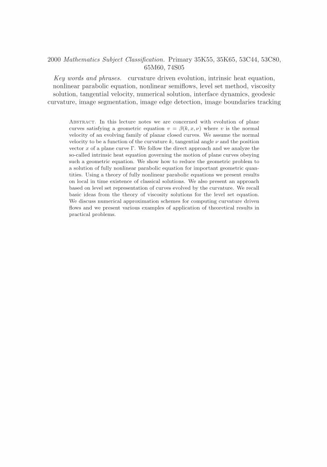
2000 Mathematics Subject Classification. Primary 35K55, 35K65, 53C44, 53C80,65M60, 74S05
Key words and phrases. curvature driven evolution, intrinsic heat equation,nonlinear parabolic equation, nonlinear semiflows, level set method, viscositysolution, tangential velocity, numerical solution, interface dynamics, geodesic
curvature, image segmentation, image edge detection, image boundaries tracking
Abstract. In this lecture notes we are concerned with evolution of planecurves satisfying a geometric equation v = β(k, x, ν) where v is the normalvelocity of an evolving family of planar closed curves. We assume the normalvelocity to be a function of the curvature k, tangential angle ν and the position
vector x of a plane curve Γ. We follow the direct approach and we analyze theso-called intrinsic heat equation governing the motion of plane curves obeyingsuch a geometric equation. We show how to reduce the geometric problem toa solution of fully nonlinear parabolic equation for important geometric quan-tities. Using a theory of fully nonlinear parabolic equations we present resultson local in time existence of classical solutions. We also present an approachbased on level set representation of curves evolved by the curvature. We recallbasic ideas from the theory of viscosity solutions for the level set equation.We discuss numerical approximation schemes for computing curvature drivenflows and we present various examples of application of theoretical results inpractical problems.

“topicsOnPartialDifferentialEquations” — 2008/1/7 — 16:30 — page 57 — #69
Contents
Preface 59
Chapter 1. Introduction 611. Mathematical models leading to curvature driven flows of planar curves 611.1. Interface dynamics 611.2. Image segmentation 621.3. Geodesic curvature driven flow of curves on a surface 632. Methodology 633. Numerical techniques 63
Chapter 2. Preliminaries 651. Notations and elements of differential geometry 652. Governing equations 673. First integrals for geometric quantities 693.1. The total length equation 693.2. The area equation 693.3. Brakke’s motion by curvature 704. Gage-Hamilton and Grayson’s theorems 704.1. Asymptotic profile of shrinking curves for other normal velocities 72
Chapter 3. Qualitative behavior of solutions 751. Local existence of smooth solutions 751.1. Local representation of an embedded curve 751.2. Nonlinear analytic semiflows 771.2.1. Maximal regularity theory 781.2.2. Application of the abstract result for the fully nonlinear parabolic
equation for the distance function 801.3. Local existence, uniqueness and continuation of classical solutions 80
Chapter 4. Level set methods for curvature driven flows of planar curves 851. Level set representation of Jordan curves in the plane 851.1. A-priori bounds for the total variation of the shape function 872. Viscosity solutions to the level set equation 883. Numerical methods 903.1. Examples from Mitchell’s Level set Matlab toolbox 90
Chapter 5. Numerical methods for the direct approach 931. A role of the choice of a suitable tangential velocity 931.1. Non-locally dependent tangential velocity functional 94
57
“topicsOnPartialDifferentialEquations” — 2008/1/7 — 16:30 — page 58 — #70
58 CONTENTS
1.2. Locally dependent tangential velocity functional 962. Flowing finite volume approximation scheme 962.0.1. Normal velocity depending on the tangent angle 972.0.2. Normal velocity depending on the tangent angle and the position
vector 100
Chapter 6. Applications of curvature driven flows 1031. Computation of curvature driven evolution of planar curves with
external force 1032. Flows of curves on a surface driven by the geodesic curvature 1032.1. Planar projection of the flow on a graph surface 1053. Applications in the theory of image segmentation 1083.1. Edge detection in static images 1083.2. Tracking moving boundaries 110
Bibliography 115
“topicsOnPartialDifferentialEquations” — 2008/1/7 — 16:30 — page 59 — #71
Preface
The lecture notes on Qualitative and quantitative aspects of curvature drivenflows of plane curves are based on the series of lectures given by the author inthe fall of 2006 during his stay at the Necas Center for Mathematical Modeling atCharles University in Prague. The principal goal was to present basic facts andknown results in this field to PhD students and young researchers of NCMM.
The main purpose of these notes is to present theoretical and practical topics inthe field of curvature driven flows of planar curves and interfaces. There are manyrecent books and lecture notes on this topic. My intention was to find a balancebetween presentation of subtle mathematical and technical details and ability ofthe material to give a comprehensive overview of possible applications in this field.This is often a hard task but I tried to find this balance.
I am deeply indebted to Karol Mikula for long and fruitful collaboration onthe problems of curvature driven flows of curves. A lot of the material presentedin these lecture notes has been jointly published with him. I want to acknowledgea recent collaboration with V. Srikrishnan who brought to my attention importantproblems arising in tracking of moving boundaries. I also wish to thank JosefMalek from NCMM of Charles University in Prague for giving me a possibility tovisit NCMM and present series of lectures and for his permanent encouragementto prepare these lecture notes.
Daniel SevcovicBratislava, July 2007.
59

“topicsOnPartialDifferentialEquations” — 2008/1/7 — 16:30 — page 60 — #72
“topicsOnPartialDifferentialEquations” — 2008/1/7 — 16:30 — page 61 — #73
CHAPTER 1
Introduction
In this lecture notes we are concerned with evolution of plane curves satisfyinga geometric equation
v = β(k, x, ν) (1.1)
where v is the normal velocity of an evolving family of planar closed curves. Weassume the normal velocity to be a function of the curvature k, tangent angle νand the position vector x of a plane curve Γ.
Geometric equations of the form (1.1) can be often found in variety of appliedproblems like e.g. the material science, dynamics of phase boundaries in thermo-mechanics, in modeling of flame front propagation, in combustion, in computationsof first arrival times of seismic waves, in computational geometry, robotics, semi-conductors industry, etc. They also have a special conceptual importance in imageprocessing and computer vision theories. A typical case in which the normal ve-locity v may depend on the position vector x can be found in image segmentation[CKS97, KKO+96]. For a comprehensive overview of other important applicationsof the geometric Eq. (1.1) we refer to recent books by Sethian, Sapiro and Osherand Fedkiw [Set96, Sap01, OF03].
1. Mathematical models leading to curvature driven flows of planarcurves
1.1. Interface dynamics. If a solid phase occupies a subset Ωs(t) ⊂ Ω anda liquid phase - a subset Ωl(t) ⊂ Ω, Ω ⊂ R2, at a time t, then the phase interfaceis the set Γt = ∂Ωs(t) ∩ ∂Ωl(t) which is assumed to be a closed smooth embeddedcurve. The sharp-interface description of the solidification process is then describedby the Stefan problem with a surface tension
ρc∂tU = λ∆U in Ωs(t) and Ωl(t),
[λ∂nU ]ls = −Lv on Γt, (1.2)
δe
σ(U − U∗) = −δ2(ν)k + δ1(ν)v on Γt, (1.3)
subject to initial and boundary conditions for the temperature field U and initialposition of the interface Γ (see e.g. [Ben01]). The constants ρ, c, λ represent materialcharacteristics (density, specific heat and thermal conductivity), L is the latent heatper unit volume, U∗ is a melting point and v is the normal velocity of an interface.Discontinuity in the heat flux on the interface Γt is described by the Stefan condition(1.2). The relationship (1.3) is referred to as the Gibbs – Thomson law on theinterface Γt, where δe is difference in entropy per unit volume between liquid andsolid phases, σ is a constant surface tension, δ1 is a coefficient of attachment kinetics
61
“topicsOnPartialDifferentialEquations” — 2008/1/7 — 16:30 — page 62 — #74
62 1. INTRODUCTION
and dimensionless function δ2 describes anisotropy of the interface. One can seethat the Gibbs–Thomson condition can be viewed as a geometric equation havingthe form (1.1). In this application the normal velocity v = β(k, x, ν) has a specialform
β = β(k, ν) = δ(ν)k + F
In the theory of phase interfaces separating solid and liquid phases, the geomet-ric equation (1.1) with β(k, x, ν) = δ(ν)k + F corresponds to the so-called Gibbs–Thomson law governing the crystal growth in an undercooled liquid [Gur93, BM98].In the series of papers [AG89, AG94, AG96]. Angenent and Gurtin studied motionof phase interfaces. They proposed to study the equation of the form
µ(ν, v)v = h(ν)k − g
where µ is the kinetic coefficient and quantities h, g arise from constitutive de-scription of the phase boundary. The dependence of the normal velocity v on thecurvature k is related to surface tension effects on the interface, whereas the depen-dence on ν (orientation of interface) introduces anisotropic effects into the model.In general, the kinetic coefficient µ may also depend on the velocity v itself givingrise to a nonlinear dependence of the function v = β(k, ν) on k and ν. If the mo-tion of an interface is very slow, then β(k, x, ν) is linear in k (cf. [AG89]) and (1.1)corresponds to the classical mean curvature flow studied extensively from both themathematical (see, e.g., [GH86, AL86, Ang90a, Gra87]) and numerical point ofview (see, e.g., [Dzi94, Dec97, MK96, NPV93, OS88]).
In the series of papers [AG89, AG96], Angenent and Gurtin studied perfectconductors where the problem can be reduced to a single equation on the interface.Following their approach and assuming a constant kinetic coefficient one obtainsthe equation
v = β(k, ν) ≡ δ(ν)k + F
describing the interface dynamics. It is often referred to as the anisotropic curveshortening equation with a constant driving force F (energy difference between bulkphases) and a given anisotropy function δ.
1.2. Image segmentation. A similar equation to (1.1) arises from the theoryof image segmentation in which detection of object boundaries in the analyzed imageplays an important role. A given black and white image can be represented by itsintensity function I : R2 → [0, 255]. The aim is to detect edges of the image, i.e.closed planar curves on which the gradient ∇I is large (see [KM95]). The ideabehind the so-called active contour models is to construct an evolving family ofplane curves converging to an edge (see [KWT87]). One can construct a family ofcurves evolved by the normal velocity v = β(k, x, ν) of the form
β(k, x, ν) = δ(x, ν)k + c(x, ν)
where c(x, ν) is a driving force and δ(x, ν) > 0 is a smoothing coefficient. Thesefunctions depend on the position vector x as well as orientation angle ν of a curve.Evolution starts from an initial curve which is a suitable approximation of the edgeand then it converges to the edge provided that δ, c are suitable chosen functions.
“topicsOnPartialDifferentialEquations” — 2008/1/7 — 16:30 — page 63 — #75
3. NUMERICAL TECHNIQUES 63
In the context of level set methods, edge detection techniques based on thisidea were first discussed by Caselles et al. and Malladi et al. in [CCCD93, MSV95].Later on, they have been revisited and improved in [CKS97, CKSS97, KKO+96].
1.3. Geodesic curvature driven flow of curves on a surface. Anotherinteresting application of the geometric equation (1.1) arises from the differentialgeometry. The purpose is to investigate evolution of curves on a given surfacedriven by the geodesic curvature and prescribed external force. We restrict ourattention to the case when the normal velocity V is a linear function of the geodesiccurvature Kg and external force F , i.e. V = Kg + F and the surface M in R3
can be represented by a smooth graph. The idea how to analyze a flow of curveson a surface M consists in vertical projection of surface curves into the plane.This allows for reducing the problem to the analysis of evolution of planar curvesinstead of surface ones. Although the geometric equation V = Kg + F is simplethe description of the normal velocity v of the family of projected planar curves israther involved. Nevertheless, it can be written in the form of equation (1.1). Theprecise form of the function β can be found in the last section.
2. Methodology
Our methodology how to solve (1.1) is based on the so-called direct approach in-vestigated by Dziuk, Deckelnick, Gage and Hamilton, Grayson, Mikula and Sevcovicand other authors (see e.g. [Dec97, Dzi94, Dzi99, GH86, Gra87, MK96, Mik97,MS99, MS01, MS04a, MS04b] and references therein). The main idea is to usethe so-called Lagrangean description of motion and to represent the flow of planarcurves by a position vector x which is a solution to the geometric equation
∂tx = β ~N + α~T
where ~N, ~T are the unit inward normal and tangent vectors, resp. It turns outthat one can construct a closed system of parabolic-ordinary differential equationsfor relevant geometric quantities: the curvature, tangential angle, local length andposition vector. Other well-known techniques, like e.g. level-set method due toOsher and Sethian [Set96, OF03] or phase-field approximations (see e.g. Caginalp,Nochetto et al., Benes [Cag90, NPV93, Ben01]) treat the geometric equation (1.1)by means of a solution to a higher dimensional parabolic problem. In compari-son to these methods, in the direct approach one space dimensional evolutionaryproblems are solved only. Notice that the direct approach for solving (1.1) can beaccompanied by a proper choice of tangential velocity α significantly improving andstabilizing numerical computations as it was documented by many authors (see e.g.[Dec97, HLS94, HKS98, Kim97, MS99, MS01, MS04a, MS04b]).
3. Numerical techniques
Analytical methods for mathematical treatment of (1.1) are strongly related tonumerical techniques for computing curve evolutions. In the direct approach oneseeks for a parameterization of the evolving family of curves. By solving the so-called intrinsic heat equation one can directly find a position vector of a curve (seee.g. [Dzi91, Dzi94, Dzi99, MS99, MS01, MS04a]). There are also other direct meth-ods based on solution of a porous medium–like equation for curvature of a curve
“topicsOnPartialDifferentialEquations” — 2008/1/7 — 16:30 — page 64 — #76
64 1. INTRODUCTION
[MK96, Mik97], a crystalline curvature approximation [Gir95, GK94, UY00], specialfinite difference schemes [Kim94, Kim97], and a method based on erosion of poly-gons in the affine invariant scale case [Moi98]. By contrast to the direct approach,level set methods are based on introducing an auxiliary function whose zero level setsrepresent an evolving family of planar curves undergoing the geometric equation(1.1) (see, e.g., [OS88, Set90, Set96, Set98, HMS98]). The other indirect method isbased on the phase-field formulations (see, e.g., [Cag90, NPV93, EPS96, BM98]).The level set approach handles implicitly the curvature-driven motion, passing theproblem to higher dimensional space. One can deal with splitting and/or merg-ing of evolving curves in a robust way. However, from the computational point ofview, level set methods are much more expensive than methods based on the directapproach.

“topicsOnPartialDifferentialEquations” — 2008/1/7 — 16:30 — page 65 — #77
CHAPTER 2
Preliminaries
The purpose of this section is to review basic facts and results concerning acurvature driven flow of planar curves. We will focus our attention on the so-calledLangrangean description of a moving curve in which we follow an evolution of pointpositions of a curve. This is also referred to as a direct approach in the context ofcurvature driven flows of planar curves ([AL86, Dzi91, Dzi94, Dec97, MK96, MS99,MS01]).
First we recall some basic facts and elements of differential geometry. Thenwe derive a system of equations for important geometric quantities like e.g. acurvature, local length and tangential angle. With help of these equations we shallbe able to derive equations describing evolution of the total length, enclosed areaof an evolving curve and transport of a scalar function quantity.
1. Notations and elements of differential geometry
An embedded regular plane curve (a Jordan curve) Γ is a closed C1 smooth onedimensional nonselfintersecting curve in the plane R2. It can be parameterized bya smooth function x : S1 → R2. It means that Γ = Img(x) := x(u), u ∈ S1 andg = |∂ux| > 0. Taking into account the periodic boundary conditions at u = 0, 1we can hereafter identify the unit circle S1 with the interval [0, 1]. The unit arc-length parameterization of a curve Γ = Img(x) is denoted by s and it satisfies|∂sx(s)| = 1 for any s. Furthermore, the arc-length parameterization is related tothe original parameterization u via the equality ds = g du. Notice that the intervalof values of the arc-length parameter depends on the curve Γ. More precisely,s ∈ [0, L(Γ)] where L(Γ) is the length of the curve Γ. Since s is the arc-length
parameterization the tangent vector ~T of a curve Γ is given by ~T = ∂sx = g−1∂ux.
We choose orientation of the unit inward normal vector ~N in such a way that
det(~T , ~N) = 1 where det(~a,~b) is the determinant of the 2 × 2 matrix with column
vectors ~a,~b. Notice that 1 = |~T |2 = (~T .~T ). Therefore, 0 = ∂s(~T .~T ) = 2(~T .∂s~T ).
Here a.b denotes the standard Euclidean scalar product in R2. Thus the direction
of the normal vector ~N must be proportional to ∂s~T . It means that there is a
real number k ∈ R such that ~N = k∂s~T . Similarly, as 1 = | ~N |2 = ( ~N. ~N) we have
0 = ∂s( ~N. ~N) = 2( ~N.∂s~N) and so ∂s
~N is collinear to the vector ~T . Since ( ~N.~T ) = 0
we have 0 = ∂s( ~N.~T ) = (∂s~N.~T ) + ( ~N.∂s
~T ). Therefore, ∂s~N = −k~T . In summary,
for the arc-length derivative of the unit tangent and normal vectors to a curve Γwe have
∂s~T = k ~N, ∂s
~N = −k~T (2.1)
65
“topicsOnPartialDifferentialEquations” — 2008/1/7 — 16:30 — page 66 — #78
66 2. PRELIMINARIES
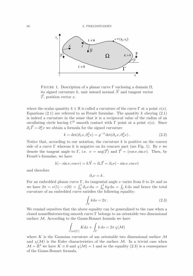
Figure 1. Description of a planar curve Γ enclosing a domain Ω,
its signed curvature k, unit inward normal ~N and tangent vector~T , position vector x.
where the scalar quantity k ∈ R is called a curvature of the curve Γ at a point x(s).Equations (2.1) are referred to as Frenet formulae. The quantity k obeying (2.1)is indeed a curvature in the sense that it is a reciprocal value of the radius of anoscullating circle having C2 smooth contact with Γ point at a point x(s). Since
∂s~T = ∂2
sx we obtain a formula for the signed curvature
k = det(∂sx, ∂2sx) = g−3 det(∂ux, ∂
2ux) . (2.2)
Notice that, according to our notation, the curvature k is positive on the convexside of a curve Γ whereas it is negative on its concave part (see Fig. 1). By ν we
denote the tangent angle to Γ, i.e. ν = arg(~T ) and ~T = (cos ν, sin ν). Then, byFrenet’s formulae, we have
k(− sin ν, cos ν) = k ~N = ∂s~T = ∂sν(− sin ν, cos ν)
and therefore
∂sν = k .
For an embedded planar curve Γ, its tangential angle ν varies from 0 to 2π and so
we have 2π = ν(1) − ν(0) =∫ 1
0∂uν du =
∫ 1
0kg du =
∫
Γk ds and hence the total
curvature of an embedded curve satisfies the following equality:∫
Γ
kds = 2π . (2.3)
We remind ourselves that the above equality can be generalized to the case when aclosed nonselfintersecting smooth curve Γ belongs to an orientable two dimensionalsurface M. According to the Gauss-Bonnet formula we have
∫
int(Γ)
Kdx+
∫
Γ
k ds = 2π χ(M)
where K is the Gaussian curvature of am orientable two dimensional surface Mand χ(M) is the Euler characteristics of the surface M. In a trivial case whenM = R2 we have K ≡ 0 and χ(M) = 1 and so the equality (2.3) is a consequenceof the Gauss-Bonnet formula.

“topicsOnPartialDifferentialEquations” — 2008/1/7 — 16:30 — page 67 — #79
2. GOVERNING EQUATIONS 67
2. Governing equations
In these lecture notes we shall assume that the normal velocity v of an evolvingfamily of plane curves Γt, t ≥ 0, is equal to a function β of the curvature k, tangentialangle ν and position vector x ∈ Γt,
v = β(x, k, ν) .
(see (1.1)). Hereafter, we shall suppose that the function β(k, x, ν) is a smoothfunction which is increasing in the k variable, i.e.
β′k(k, x, ν) > 0 .
An idea behind the direct approach consists of representation of a family of embed-ded curves Γt by the position vector x ∈ R2, i.e.
Γt = Img(x(., t)) = x(u, t), u ∈ [0, 1]where x is a solution to the geometric equation
∂tx = β ~N + α~T (2.4)
where β = β(x, k, ν), ~N = (− sin ν, cos ν) and ~T = (cos ν, sin ν) are the unit in-
ward normal and tangent vectors, respectively. For the normal velocity v = ∂tx. ~Nwe have v = β(x, k, ν). Notice that the presence of arbirary tangential velocityfunctional α has no impact on the shape of evolving curves.
The goal of this section is to derive a system of PDEs governing the evolution ofthe curvature k of Γt = Img(x(., t)), t ∈ [0, T ), and some other geometric quantitieswhere the family of regular plane curves where x = x(u, t) is a solution to theposition vector equation (2.4). These equations will be used in order to derive apriori estimates of solutions. Notice that such an equation for the curvature iswell known for the case when α = 0, and it reads as follows: ∂tk = ∂2
sβ + k2β (cf.[GH86, AG89]). Here we present a brief sketch of the derivation of the correspondingequations for the case of a nontrivial tangential velocity α.
Let us denote ~p = ∂ux. Since u ∈ [0, 1] is a fixed domain parameter wecommutation relation ∂t∂u = ∂u∂t. Then, by using Frenet’s formulae, we obtain
∂t~p = |∂ux|((∂sβ + αk) ~N + (−βk + ∂sα)~T ),
~p . ∂t~p = |∂ux| ~T . ∂t~p = |∂ux|2(−βk + ∂sα), (2.5)
det(~p, ∂t~p) = |∂ux| det(~T , ∂t~p) = |∂ux|2 (∂sβ + αk),
det(∂t~p, ∂u~p) = −|∂ux|∂u|∂ux|(∂sβ + αk) + |∂ux|3 (−βk + ∂sα),
because ∂u~p = ∂2ux = ∂u(|∂ux| ~T ) = ∂u|∂ux| ~T + k|∂ux|2 ~N . Since ∂u det(~p, ∂t~p) =
det(∂u~p, ∂t~p)+det(~p, ∂u∂t~p), we have det(~p, ∂u∂t~p) = ∂u det(~p, ∂t~p)+det(∂t~p, ∂u~p).As k = det(~p, ∂u~p) |~p|−3 (see (2.2)), we obtain
∂tk = −3|p|−5(~p . ∂t~p) det(~p, ∂u~p) + |~p|−3 (det(∂t~p, ∂u~p) + det(~p, ∂u∂t~p))
= −3k|~p|−2(~p . ∂t~p) + 2|~p|−3 det(∂t~p, ∂u~p) + |~p|−3∂u det(~p, ∂t~p).
Finally, by applying identities (2.5), we end up with the second-order nonlinearparabolic equation for the curvature:
∂tk = ∂2sβ + α∂sk + k2β . (2.6)
“topicsOnPartialDifferentialEquations” — 2008/1/7 — 16:30 — page 68 — #80
68 2. PRELIMINARIES
The identities (2.5) can be used in order to derive an evolutionary equation forthe local length |∂ux|. Indeed, ∂t|∂ux| = (∂ux . ∂u∂tx)/|∂ux| = (~p . ∂t~p)/|∂ux|. By(2.5) we have the
∂t|∂ux| = −|∂ux| kβ + ∂uα (2.7)
where (u, t) ∈ QT = [0, 1]× [0, T ). In other words, ∂tds = (−kβ+ ∂sα)ds. It yieldsthe commutation relation
∂t∂s − ∂s∂t = (kβ − ∂sα)∂s. (2.8)
Next we derive equations for the time derivative of the unit tangent vector ~T andtangent angle ν. Using the above commutation relation and Frenet formulae weobtain
∂t~T = ∂t∂sx = ∂s∂tx+ (kβ − ∂sα)∂sx ,
= ∂s(β ~N + α~T ) + (kβ − ∂sα)~T ,
= (∂sβ + αk) ~N .
Since ~T = (cos ν, sin ν) and ~N = (− sin ν, cos ν) we conclude that ∂tν = ∂sβ + αk.Summarizing, we end up with evolutionary equations for the unit tangent and
normal vectors ~T , ~N and the tangent angle ν
∂t~T = (∂sβ + αk) ~N ,
∂t~N = −(∂sβ + αk)~T , (2.9)
∂tν = ∂sβ + αk .
Since ∂sν = k and ∂sβ = β′k∂sk + β′
νk + ∇xβ.~T we obtain the following closedsystem of parabolic-ordinary differential equations:
∂tk = ∂2sβ + α∂sk + k2β , (2.10)
∂tν = β′k∂
2sν + (α+ β′
ν)∂sν + ∇xβ.~T , (2.11)
∂tg = −gkβ + ∂uα , (2.12)
∂tx = β ~N + α~T , (2.13)
where (u, t) ∈ QT = [0, 1] × (0, T ), ds = g du and ~T = ∂sx = (cos ν, sin ν), ~N =~T⊥ = (− sin ν, cos ν). The functional α may depend on the variables k, ν, g, x. Asolution (k, ν, g, x) to (2.10) – (2.13) is subject to initial conditions
k(., 0) = k0 , ν(., 0) = ν0 , g(., 0) = g0 , x(., 0) = x0(.) ,
and periodic boundary conditions at u = 0, 1 except of the tangent angle ν for which
we require that the tangent vector ~T (u, t) = (cos(ν(u, t)), sin(ν(u, t))) is 1-periodicin the u variable, i.e. ν(1, t) = ν(0, t) + 2π. Notice that the initial conditions fork0, ν0, g0 and x0 (the curvature, tangent angle, local length element and positionvector of the initial curve Γ0) must satisfy the following compatibility constraints:
g0 = |∂ux0| > 0 , k0 = det(g−30 ∂ux0, ∂
2ux0) , ∂uν0 = g0k0 .
“topicsOnPartialDifferentialEquations” — 2008/1/7 — 16:30 — page 69 — #81
3. FIRST INTEGRALS FOR GEOMETRIC QUANTITIES 69
3. First integrals for geometric quantities
The aim of this section is to derive basic identities for various geometric quan-tities like e.g. the length of a closed curve and the area enclosed by a Jordan curvein the plane. These identities (first integrals) will be used later in the analysis ofthe governing system of equations.
3.1. The total length equation. By integrating (2.7) over the interval [0, 1]and taking into account that α satisfies periodic boundary conditions, we obtainthe total length equation
d
dtLt +
∫
Γt
kβds = 0, (2.14)
where Lt = L(Γt) is the total length of the curve Γt, Lt =∫
Γt ds =∫ 1
0|∂ux(u, t)| du.
If kβ ≥ 0, then the evolution of planar curves parameterized by a solution of (1.1)represents a curve shortening flow, i.e., Lt2 ≤ Lt1 ≤ L0 for any 0 ≤ t1 ≤ t2 ≤ T .The condition kβ ≥ 0 is obviously satisfied in the case β(k, ν) = γ(ν)|k|m−1k, wherem > 0 and γ is a nonnegative anisotropy function. In particular, the Euclideancurvature driven flow (β = k) is curve shortening flow.
3.2. The area equation. Let us denote by A = At the area of the domainΩt enclosed by a Jordan curve Γt. Then by using Green’s formula we obtain, forP = −x2/2, Q = x1/2,
At =
∫∫
Ωt
dx =
∫∫
Ωt
∂Q
∂x1− ∂P
∂x2dx =
∮
Γt
Pdx1 +Qdx2 =1
2
∮
Γt
−x2dx1 + x1dx2 .
Since dxi = ∂uxidu, u ∈ [0, 1], we have
At =1
2
∫ 1
0
det(x, ∂ux) du .
Clearly, integration of the derivative of a quantity along a closed curve yields zero.
Therefore 0 =∫ 1
0∂u det(x, ∂tx)du =
∫ 1
0det(∂ux, ∂tx) + det(x, ∂u∂tx)du, and so
∫ 1
0 det(x, ∂u∂tx)du =∫ 1
0 det(∂tx, ∂ux)du because det(∂ux, ∂tx) = − det(∂tx, ∂ux).
As ∂tx = β ~N + α~T , ∂uxdu = ~Tds and ddtAt = 1
2
∫ 1
0 2 det(∂tx, ∂ux)du we can
conclude that
d
dtAt +
∫
Γt
βds = 0. (2.15)
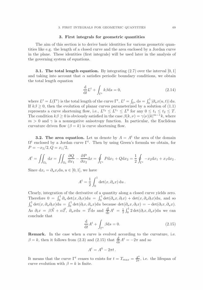
Remark. In the case when a curve is evolved according to the curvature, i.e.
β = k, then it follows from (2.3) and (2.15) that ddtAt = −2π and so
At = A0 − 2πt .
It means that the curve Γt ceases to exists for t = Tmax = A0
2π , i.e. the lifespan ofcurve evolution with β = k is finite.
“topicsOnPartialDifferentialEquations” — 2008/1/7 — 16:30 — page 70 — #82
70 2. PRELIMINARIES
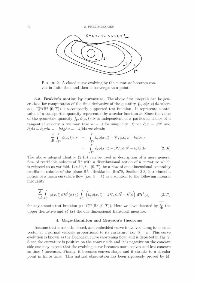
Figure 2. A closed curve evolving by the curvature becomes con-vex in finite time and then it converges to a point.
3.3. Brakke’s motion by curvature. The above first integrals can be gen-eralized for computation of the time derivative of the quantity
∫
Γt φ(x, t) ds where
φ ∈ C∞0 (R2, [0, T )) is a compactly supported test function. It represents a total
value of a transported quantity represented by a scalar function φ. Since the valueof the geometric quantity
∫
Γt φ(x, t) ds is independent of a particular choice of a
tangential velocity α we may take α = 0 for simplicity. Since ∂tx = β ~N and∂tds = ∂tgdu = −kβgdu = −kβds we obtain
d
dt
∫
Γt
φ(x, t) ds =
∫
Γt
∂tφ(x, t) + ∇xφ.∂tx− kβφds
=
∫
Γt
∂tφ(x, t) + β∇xφ. ~N − kβφds . (2.16)
The above integral identity (2.16) can be used in description of a more generalflow of rectifiable subsets of R2 with a distributional notion of a curvature whichis refereed to as varifold. Let Γt, t ∈ [0, T ), be a flow of one dimensional countablyrectifiable subsets of the plane R2. Brakke in [Bra78, Section 3.3] introduced anotion of a mean curvature flow (i.e. β = k) as a solution to the following integralinequality
d
dt
∫
Γt
φ(x, t) dH1(x) ≤∫
Γt
(
∂tφ(x, t) + k∇xφ. ~N − k2φ)
dH1(x) (2.17)
for any smooth test function φ ∈ C∞0 (R2, [0, T )). Here we have denoted by d
dtthe
upper derivative and H1(x) the one dimensional Hausdorff measure.
4. Gage-Hamilton and Grayson’s theorems
Assume that a smooth, closed, and embedded curve is evolved along its normalvector at a normal velocity proportional to its curvature, i.e. β = k. This curveevolution is known as the Euclidean curve shortening flow, and is depicted in Fig. 2.Since the curvature is positive on the convex side and it is negative on the concaveside one may expect that the evolving curve becomes more convex and less concaveas time t increases. Finally, it becomes convex shape and it shrinks to a circularpoint in finite time. This natural observation has been rigorously proved by M.
“topicsOnPartialDifferentialEquations” — 2008/1/7 — 16:30 — page 71 — #83
4. GAGE-HAMILTON AND GRAYSON’S THEOREMS 71
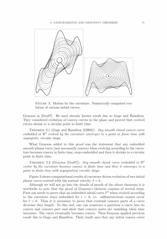
Figure 3. Motion by the curvature. Numerically computed evo-lution of various initial curves.
Grayson in [Gra87]. He used already known result due to Gage and Hamilton.They considered evolution of convex curves in the plane and proved that evolvedcurves shrink to a circular point in finite time.
Theorem 2.1 (Gage and Hamilton [GH86]). Any smooth closed convex curveembedded in R2 evolved by the curvature converges to a point in finite time withasymptotic circular shape.
What Grayson added to this proof was the statement that any embeddedsmooth planar curve (not necessarily convex) when evolving according to the curva-ture becomes convex in finite time, stays embedded and then it shrinks to a circularpoint in finite time.
Theorem 2.2 (Grayson [Gra87]). Any smooth closed curve embedded in R2
evolve by the curvature becomes convex in finite time and then it converges to apoint in finite time with asymptotical circular shape.
Figure 3 shows computational results of curvature driven evolution of two initialplanar curve evolved with the normal velocity β = k.
Although we will not go into the details of proofs of the above theorems it isworthwile to note that the proof of Grayson’s theorem consists of several steps.First one needs to prove that an embedded initial curve Γ0 when evolved accordingto the curvature stays embedded for t > 0, i.e. selfintersections cannot occurfor t > 0. Then it is necessary to prove that eventual concave parts of a curvedecrease they length. To this end, one can construct a partition a curve into itsconvex and concave part and show that concave parts are vanishing when timeincreases. The curve eventually becomes convex. Then Grayson applied previousresult due to Gage and Hamilton. Their result says that any initial convex curve
“topicsOnPartialDifferentialEquations” — 2008/1/7 — 16:30 — page 72 — #84
72 2. PRELIMINARIES
asymptotically approaches a circle when t→ Tmax where Tmax is finite. To interprettheir result in the language of parabolic partial differential equations we notice thatthe solution to (2.10) with β = k remains positive provided that the initial valuek0 was nonnegative. This is a direct consequence of the maximum principle forparabolic equations. Indeed, let us denote by y(t) = minΓt k(., t). With regardto the envelope theorem we may assume that there exists s(t) such that y(t) =k(s(t), t). As ∂2
sk ≥ 0 and ∂sk = 0 at s = s(t) we obtain from (2.10) that y′(t) ≥y3(t). Solving this ordinary differential inequality with positive initial conditiony(0) = minΓ0 k0 > 0 we obtain minΓt k(., t) = y(t) > 0 for 0 < t < Tmax. Thus Γt
remains convex provided Γ0 was convex. The proof of the asymptotic circular profileis more complicated. However, it can be very well understood when consideringselfsimilarly rescaled dependent and independent variables in equation (2.10). Inthese new variables, the statement of Gage and Hamilton theorem is equivalent tothe proof of asymptotical stability of the constant unit solution.
In the proof of Grayson’s theorem one can find another nice application ofthe parabolic comparison principle. Namely, if one wants to prove embeddednesproperty of an evolved curve Γt it is convenient to inspect the following distancefunction between arbitrary two points x(s1, t), x(s2, t) of a curve Γt:
f(s1, s2, t) = |x(s1, t) − x(s2, t)|2
where s1, s2 ∈ [0, L(Γt)] and t > 0. Assume that x = x(s, t) satisfies (2.4). Withoutloss of generality we may assume α = 0 as α does not change the shape of thecurve. Hence the embeddednes property is independent of α. Let us computepartial derivatives of f with respect to its variables. With help of Frenet formulaewe obtain
∂tf = 2((x(s1, t) − x(s2, t)).(∂tx(s1, t) − ∂tx(s2, t)))
= 2((x(s1, t) − x(s2, t)).(k(s1, t) ~N(s1, t) − k(s2, t) ~N(s2, t)))
∂s1f = 2((x(s1, t) − x(s2, t)). ~T (s1, t))
∂s2f = −2((x(s1, t) − x(s2, t)). ~T (s2, t))
∂2s1f = 2(~T (s1, t). ~T (s1, t)) + 2k(s1, t)((x(s1, t) − x(s2, t)). ~N(s1, t))
∂2s2f = 2(~T (s1, t). ~T (s1, t)) − 2k(s2, t)((x(s1, t) − x(s2, t). ~N(s2, t)) .
Hence∂tf = ∆f − 4
where ∆ is the Laplacian operator with respect to variables s1, s2. Using a cleverapplication of a suitable barrier function (a circle) and comparison principle forthe above parabolic equation Grayson proved that f(s1, s2, t) ≥ δ > 0 whenever|s1 − s2| ≥ ǫ > 0 where ǫ, δ > 0 are sufficiently small. But this is equivalent to thestatement that the curve Γt is embedded. Notice that the above ”trick” works onlyfor the case β = k and this is why it is still an open question whether embeddedinitial curve remains embedded when it is evolved by a general normal velocityβ = β(k).
4.1. Asymptotic profile of shrinking curves for other normal veloci-ties. There are some partial results in this direction. If β = k1/3 then the corre-sponding flow of planar curves is called affine space scale flow. It has been studied
“topicsOnPartialDifferentialEquations” — 2008/1/7 — 16:30 — page 73 — #85
4. GAGE-HAMILTON AND GRAYSON’S THEOREMS 73
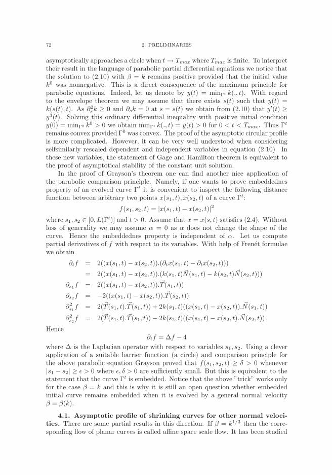
Figure 4. An initial ellipse evolved with the normal velocity β = k1/3.
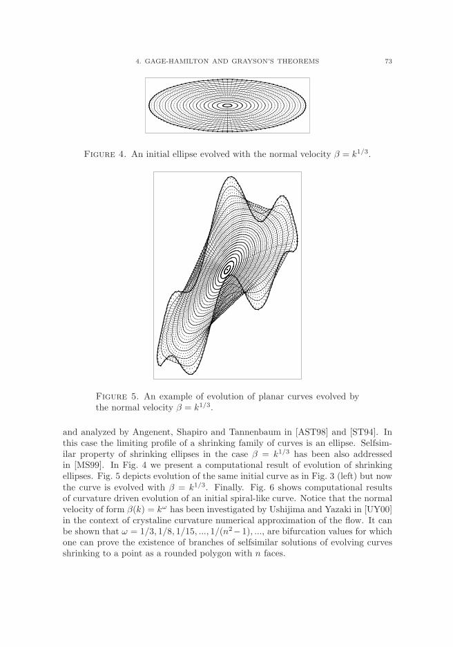
Figure 5. An example of evolution of planar curves evolved bythe normal velocity β = k1/3.
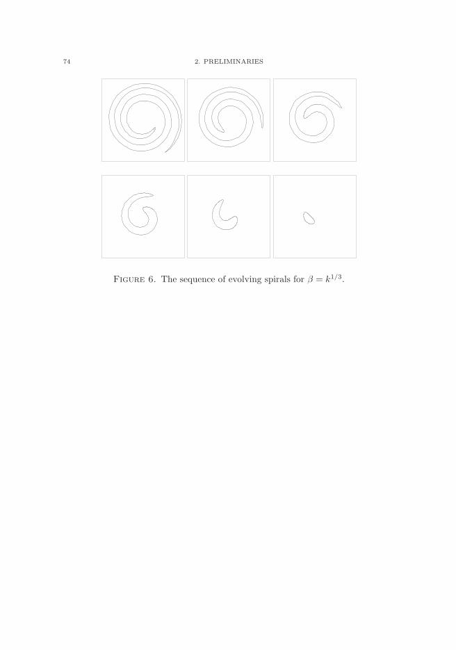
and analyzed by Angenent, Shapiro and Tannenbaum in [AST98] and [ST94]. Inthis case the limiting profile of a shrinking family of curves is an ellipse. Selfsim-ilar property of shrinking ellipses in the case β = k1/3 has been also addressedin [MS99]. In Fig. 4 we present a computational result of evolution of shrinkingellipses. Fig. 5 depicts evolution of the same initial curve as in Fig. 3 (left) but nowthe curve is evolved with β = k1/3. Finally. Fig. 6 shows computational resultsof curvature driven evolution of an initial spiral-like curve. Notice that the normalvelocity of form β(k) = kω has been investigated by Ushijima and Yazaki in [UY00]in the context of crystaline curvature numerical approximation of the flow. It canbe shown that ω = 1/3, 1/8, 1/15, ..., 1/(n2− 1), ..., are bifurcation values for whichone can prove the existence of branches of selfsimilar solutions of evolving curvesshrinking to a point as a rounded polygon with n faces.
“topicsOnPartialDifferentialEquations” — 2008/1/7 — 16:30 — page 74 — #86
74 2. PRELIMINARIES
Figure 6. The sequence of evolving spirals for β = k1/3.
“topicsOnPartialDifferentialEquations” — 2008/1/7 — 16:30 — page 75 — #87
CHAPTER 3
Qualitative behavior of solutions
In this chapter we focus our attention on qualitative behavior of curvaturedriven flows of planar curves. We present techniques how to prove local in timeexistence of a smooth family of curves evolved with the normal velocity given bya general function β = β(k, x, ν) depending on the curvature k, position vector xas well as the tangential angle ν. The main idea is to transform the geometricproblem into the language of a time depending solution to an evolutionary partialdifferential equation like e.g. (2.10)–(2.13). First we present an approach due toAngenent describing evolution of an initial curve by a fully nonlinear parabolicequation for the distance function measuring the normal distance of the initialcurve Γ0 the evolved curve Γt for small values of t > 0. The second approachpresented in this chapter is based on solution to the system of nonlinear parabolic-ordinary differential equations (2.10)–(2.13) also proposed by Angenent and Gurtin[AG89, AG94] and further analyzed and applied by Mikula and Sevcovic in the seriesof papers [MS01, MS04a, MS04b]. Both approaches are based on the solution to acertain fully nonlinear parabolic equation or system of equations. To provide a localexistence and continuation result we have apply the theory of nonlinear analyticsemiflows due to Da Prato and Grisvard, Lunardi [DPG75, DPG79, Lun82] andAngenent [Ang90a, Ang90b].
1. Local existence of smooth solutions
The idea of the proof of a local existence of an evolving family of closed embed-ded curves is to transform the geometric problem into a solution to a fully nonlinearparabolic equation for the distance φ(u, t) of a point x(u, t) ∈ Γt from its initialvalue position x0(u) = x(u, 0) ∈ Γ0. This idea is due to Angenent [Ang90b] whoderived the fully nonlinear parabolic equation for φ and proved local existence ofsmooth solutions by method of abstract nonlinear evolutionary equations in Banachspaces [Ang90b].
1.1. Local representation of an embedded curve. Let Γ0 = Img(x0) bea smooth initial Jordan curve embedded in R2. Because of its smoothness andembeddednes one can construct a local parameterization of any smooth curve Γt =Img(x(., t)) lying in the thin tubular neighborhood along Γ0, i.e. distH(Γt,Γ0) < εwhere distH is the Hausdorff set distance function. This is why there exists a smallnumber 0 < ε ≪ 1 and a smooth immersion function σ : S1 × (−ε, ε) → R
2 suchthat
• x0(u) = σ(u, 0) for any u ∈ S1
75

“topicsOnPartialDifferentialEquations” — 2008/1/7 — 16:30 — page 76 — #88
76 3. QUALITATIVE BEHAVIOR OF SOLUTIONS
Figure 1. Description of a local parameterization of an embeddedcurve Γt in the neighborhood of the initial curve Γ0.
• for any u ∈ S1 there exists a unique φ = φ(u, t) ∈ (−ε, ε) such thatσ(u, φ(u, t)) = x(u, t).
• the implicitly defined function φ = φ(u, t) is smooth in its variables pro-vided the function x = x(u, t) is smooth.
It is easy to verify that the function σ(u, φ) = x0(u) + φ ~N0(u) is the immersion
having the above properties. Here ~N0(u) is the unit inward vector to the curve Γ0
at the point x0(u) (see Fig. 1).Now we can evaluate ∂tx, ∂ux, ∂
2ux and |∂ux| as follows:
∂tx = σ′φ∂tφ ,
∂ux = σ′u + σ′
φ∂uφ ,
∂2ux = σ′′
uu + 2σ′′uφ∂uφ+ σ′′
φφ(∂uφ)2 + σ′φ∂
2uφ ,
g = |∂ux| =(|σ′
u|2 + 2(σ′u.σ
′φ)∂uφ+ |σ′
φ|2(∂uφ)2) 1
2 .
Hence we can express the curvature k = det(∂ux, ∂2ux)/|∂ux|3 as follows:
g3k = det(∂ux, ∂2ux) = ∂2
uφ∂uφdet(σ′φ, σ
′φ) + ∂2
uφdet(σ′u, σ
′φ)
+ (∂uφ)2[det(σ′
u, σ′′φφ) + ∂uφdet(σ′
φ, σ′′φφ)]+ 2∂uφdet(σ′
u, σ′′uφ)
+ 2(∂uφ)2 det(σ′φ, σ
′′uφ) + det(σ′
u, σ′′uu) + ∂uφdet(σ′
φ, σ′′uu) .
Clearly, det(σ′φ, σ
′φ) = 0. Since σ′
φ = ~N0 and σ′u = ∂ux
0 + φ∂u~N0 = g0(1 − k0φ)~T 0
we have det(σ′u, σ
′φ) = g0(1 − k0φ) and (σ′
u.σ′φ) = 0. Therefore the local length
g = |∂ux| and the curvature k can be expressed as
g = |∂ux| =((g0(1 − k0φ))2 + (∂uφ)2
) 12 ,
k =g0(1 − k0φ)
g3∂2
uφ+R(u, φ, ∂uφ)
where R(u, φ, ∂uφ) is a smooth function.We proceed with evaluation of the time derivative ∂tx. Since ∂ux = σ′
u +σ′φ∂uφ
we have ~T = 1g (σ′
u +σ′φ∂uφ). The vectors ~N and ~T are perpendicular to each other.
Thus
∂tx. ~N = − det(∂tx, ~T ) =1
gdet(σ′
u, σ′φ)∂tφ =
g0(1 − k0φ)
g∂tφ
“topicsOnPartialDifferentialEquations” — 2008/1/7 — 16:30 — page 77 — #89
1. LOCAL EXISTENCE OF SMOOTH SOLUTIONS 77
because det(σ′φ, σ
′φ) = 0. Hence, a family of embedded curves Γt, t ∈ [0, T ), evolves
according to the normal velocity
β = µk + c
if and only if the function φ = φ(u, t) is a solution to the nonlinear parabolicequation
∂tφ =µ
g2∂2
uφ+g
g0(1 − k0φ)(µR(u, φ, ∂uφ) + c)
where
g =(|g0|2(1 − k0φ)2 + (∂uφ)2
) 12 .
In a general case when the normal velocity β = β(k, x, ~N) is a function of curvature
k, position vector x and the inward unit normal vector ~N , φ is a solution to a fullynonlinear parabolic equation of the form:
∂tφ = F (∂2uφ, ∂uφ, φ, u), u ∈ S1, t ∈ (0, T ) . (3.1)
The right-hand side function F = F (q, p, φ, u) is C1 is a smooth function of itsvariables and
∂F
∂q=β′
k
g2> 0
and so equation (3.1) is a nonlinear strictly parabolic equation. Equation (3.1) issubject to an initial condition
φ(u, 0) = φ0(u) ≡ 0 , u ∈ S1 . (3.2)
1.2. Nonlinear analytic semiflows. In this section we recall basic facts fromthe theory of nonlinear analytic semiflows which can be used in order to prove localin time existence of a smooth solutions to the fully nonlinear parabolic equation(3.1) subject to the initial condition (3.2). The theory has been developed by S.Angenent in [Ang90b] and A. Lunardi in [Lun82].
Equation (3.1) can be rewritten as an abstract evolutionary equation
∂tφ = F(φ) (3.3)
subject to the initial condition
φ(0) = φ0 ∈ E1 (3.4)
where F is a C1 smooth mapping between two Banach spaces E1, E0, i.e. F ∈C1(E1, E0). For example, if we take
E0 = h(S1), E1 = h2+(S1) ,
where hk+(S1), k = 0, 1, ..., is a little Holder space, i.e. the closure of C∞(S1) inthe topology of the Holder space Ck+σ(S1) (see [Ang90b]), then the mapping Fdefined as in the right-hand side of (3.1) is indeed a C1 mapping from E1 into E0.Its Frechet derivative dF(φ0) is being given by the linear operator
dF(φ0)φ = a0∂2uφ+ b0∂uφ+ c0φ
where
a0 = F ′q(∂
2uφ
0, ∂uφ0, φ0, u) =
β′k
(g0)2, b0 = F ′
p(∂2uφ
0, ∂uφ0, φ0, u),
c0 = F ′φ(∂2
uφ0, ∂uφ
0, φ0, u) .

“topicsOnPartialDifferentialEquations” — 2008/1/7 — 16:30 — page 78 — #90
78 3. QUALITATIVE BEHAVIOR OF SOLUTIONS
Suppose that the initial curve Γ0 = Img(x0) is sufficiently smooth, x0 ∈(h2+(S1)
)2and regular, i.e. g0(u) = |∂ux
0(u)| > 0 for any u ∈ S1. Then
a0 ∈ h1+(S1). A standard result from the theory of analytic semigroups (c.f.[Hen81]) enables us to conclude that the principal part A := a0∂2
u of the lineariza-tion dF(φ0) is a generator of a analytic semigroup exp(tA), t ≥ 0, in the Banachspace E0 = h(S1).
1.2.1. Maximal regularity theory. In order to proceed with the proof of localin time existence of a classical solution to the abstract nonlinear equation (3.3) wehave to recall a notion of a maximal regularity pair of Banach spaces.
Assume that (E1, E0) is a pair of Banach spaces with E1 densely included intoE0. By L(E1, E0) we shall denote the Banach space of all linear bounded operatorsfrom E1 into E0. An operator A ∈ L(E1, E0) can be considered as an unboundedoperator in the Banach space E0 with a dense domain D(A) = E1. By Hol(E1, E0)we shall denote a subset of L(E1, E0) consisting of all generators A of an analyticsemigroup exp(tA), t ≥ 0, of linear operators in the Banach space E0 (c.f. [Hen81]).
The next lemma is a standard perturbation result concerning the class of gen-erators of analytic semigroups.
Lemma 3.1. [Paz83, Theorem 2.1] The set Hol(E1, E0) is an open subset ofthe Banach space L(E1, E0).
The next result is also related to the perturbation theory for the class of gen-erators of analytic semigroups.
Definition 3.2. We say that the linear bounded operator B : E1 → E0 has arelative zero norm if for any ε > 0 there is a constant kε > 0 such that
‖Bx‖E0 ≤ ε‖x‖E1 + kε‖x‖E0
for any x ∈ E1.
As an example of such an operator we may consider an operator B ∈ L(E1, E0)satisfying the following inequality of Gagliardo-Nirenberg type:
‖Bx‖E0 ≤ C‖x‖λE1
‖x‖1−λE0
for any x ∈ E1 where λ ∈ (0, 1). Then using Young’s inequality
ab ≤ ap
p+bq
q,
1
p+
1
q= 1 ,
with p = 1/λ and q = 1/(1− λ). it is easy to verify that B has zero relative norm.
Lemma 3.3. [Paz83, Section 2.1] The set Hol(E1, E0) is closed with respect toperturbations by linear operators with zero relative norm, i.e. if A ∈ Hol(E1, E0)and B ∈ L(E1, E0) has zero relative norm then A+B ∈ Hol(E1, E0).
Neither the theory of C0 semigroups (c.f. Pazy [Paz83]) nor the theory ofanalytic semigroups (c.f. Henry [Hen81]) are able to handle fully nonlinear parabolicequations. This is mainly due to the method of integral equation which is suitablefor semilinear equations only. The second reason why these methods cannot providea local existence result is due to the fact that semigroup theories are working withfunction spaces which are fractional powers of the domain of a generator of an
“topicsOnPartialDifferentialEquations” — 2008/1/7 — 16:30 — page 79 — #91
1. LOCAL EXISTENCE OF SMOOTH SOLUTIONS 79
analytic semigroup (see [Hen81]). Therefore we need a more robust theory capableof handling fully nonlinear parabolic equations. This theory is due to Angenentand Lunardi [Ang90a, Lun82] and it is based on abstract results by Da Prato andGrisvard [DPG75, DPG79]. The basic idea is the linearization technique where onecan linearize the fully nonlinear equation at the initial condition φ0. Then one setsup a linearized semilinear equation with the right hand side which is of the secondorder with respect to deviation from the initial condition. In what follows, we shallpresent key steps of this method. First we need to introduce the maximal regularityclass which will enable us to construct an inversion operator to a nonhomogeneoussemilinear equation.
Let E = (E1, E0) be a pair of Banach spaces for which E1 is densely includedin E0. Let us define the following function spaces
X = C([0, 1], E0), Y = C([0, 1], E1) ∩ C1([0, 1], E0) .
We shall identify ∂t with the bounded differentiation operator from Y to X definedby (∂tφ)(t) = φ′(t). For a given linear bounded operator A ∈ L(E1, E0) we definethe extended operator A : Y → X × E1 defined by Aφ = (∂tφ − Aφ, φ(0)). Nextwe define a class M1(E) as follows:
M1(E) = A ∈ Hol(E), A is an isomorphism between Y and X × E1 .It means that the class M1(E) consist of all generators of analytic semigroups Asuch that the initial value problem for the semilinear evolution equation
∂tφ−Aφ = f(t), φ(0) = φ0,
has a unique solution φ ∈ Y for any right-hand side f ∈ X and the initial conditionφ0 ∈ E1 (c.f. [Ang90a]). For such an operator A we obtain boundedness of theinverse of the operator φ 7→ (∂t − A)φ mapping the Banach space Y (0) = φ ∈Y, φ(0) = 0 onto the Banach space X , i.e.
‖(∂t −A)−1‖L(X,Y (0)) ≤ C <∞ .
The class M1(E) is refereed to as maximal regularity class for the pair of Banachspaces E = (E1, E0).
An analogous perturbation result to Lemma 3.3 has been proved by Angenent.
Lemma 3.4. [Ang90a, Lemma 2.5] The set M1(E1, E0) is closed with respectto perturbations by linear operators with zero relative norm.
Using properties of the class M1(E) we are able to state the main result onthe local existence of a smooth solution to the abstract fully nonlinear evolutionaryproblem (3.3)–(3.4).
Theorem 3.5. [Ang90a, Theorem 2.7] Assume that F is a C1 mapping fromsome open subset O ⊂ E1 of the Banach space E1 into the Banach space E0. Ifthe Frechet derivative A = dF(φ) belongs to M1(E) for any φ ∈ O and the initialcondition φ0 belongs to O then the abstract fully nonlinear evolutionary problem(3.3)–(3.4) has a unique solution φ ∈ C1([0, T ], E0) ∩ C([0, T ], E1) on some smalltime interval [0, T ], T > 0.
“topicsOnPartialDifferentialEquations” — 2008/1/7 — 16:30 — page 80 — #92
80 3. QUALITATIVE BEHAVIOR OF SOLUTIONS
Proof. The proof is based on the Banach fixed point theorem. Without lossof generality (by shifting the solution φ(t) 7→ φ0 + φ(t)) we may assume φ0 = 0.Taylor’s series expansion of F at φ = 0 yields F(φ) = F0 + Aφ + R(φ) whereF0 ∈ E0, A ∈ M1(E) and the remainder function R is quadratically small, i.e.‖R(φ)‖E0 = O(‖φ‖2
E1) for small ‖φ‖E1 . Problem (3.3)–(3.4) is therefore equivalent
to the fixed point problem
φ = (∂t −A)−1(R(φ) + F0)
on the Banach space Y(0)T = φ ∈ C1([0, T ], E0) ∩ C([0, T ], E1), φ(0) = 0. Using
boundedness of the operator (∂t−A)−1 and taking T > 0 sufficiently one can provethat the right hand side of the above equation is a contraction mapping on the
space Y(0)T proving thus the statement of theorem.
1.2.2. Application of the abstract result for the fully nonlinear parabolic equationfor the distance function. Now we are in a position to apply the abstract resultcontained in Theorem 3.5 to the fully nonlinear parabolic equation (3.1) for thedistance function φ subject to a zero initial condition φ0 = 0. Notice that one hasto carefully choose function spaces to work with. Baillon in [Bai80] showed that,if we exclude the trivial case E1 = E0, the class M1(E1, E0) is nonempty only ifthe Banach space E0 contains a closed subspace isomorphic to the sequence space(c0). As a consequence of this criterion we conclude that M1(E1, E0) is empty forany reflexive Banach space E0. Therefore the space E0 cannot be reflexive. Onthe other hand, one needs to prove that the linearization A = dF(φ) : E1 → E0
generates an analytic semigroup in E0. Therefore it is convenient to work withlittle Holder spaces satisfying these structural assumptions.
Applying the abstract result from Theorem 3.5 we are able to state the followingtheorem which is a special case of a more general result by Angenent [Ang90b,Theorem 3.1] to evolution of planar curves.
Theorem 3.6. [Ang90b, Theorem 3.1] Assume that the normal velocity β =β(k, ν) is a C1,1 smooth function such that β′
k > 0 for all k ∈ R and ν ∈ [0, 2π].Let Γ0 be an embedded smooth curve with Holder continuous curvature. Then thereexists a unique maximal solution Γt, t ∈ [0, Tmax), consisting of curves evolving withthe normal velocity equal to β(k, ν).
Remark. Verification of nonemptyness of the set M1(E1, E0) might be difficultfor a particular choice of Banach pair (E1, E0). There is however a general con-struction of the Banach pair (E1, E0) such that a given linear operator A belongsto M1(E1, E0). Let F = (F1, F0) be a Banach pair. Assume that A ∈ Hol(F1, F0).We define the Banach space F2 = φ ∈ F1, Aφ ∈ F1 equipped with the graphnorm ‖φ‖F2 = ‖φ‖F1 + ‖Aφ‖F1 . For a fixed σ ∈ (0, 1) we introduce the continuousinterpolation spaces E0 = Fσ = (F1, F0)σ and E1 = F1+σ = (F2, F1)σ. Then, byresult due to Da Prato and Grisvard [DPG75, DPG79] we have A ∈ M1(E1, E0).
1.3. Local existence, uniqueness and continuation of classical solu-tions. In this section we present another approach for the proof a of a localexistence of a classical solution. Now we put our attention to a solution of thesystem of parabolic-ordinary differential equations (2.10) – (2.13). Let a regularsmooth initial curve Γ0 = Img(x0) be given. Recall that a family of planar curves
“topicsOnPartialDifferentialEquations” — 2008/1/7 — 16:30 — page 81 — #93
1. LOCAL EXISTENCE OF SMOOTH SOLUTIONS 81
Γt = Img(x(., t)), t ∈ [0, T ), satisfying (1.1) can be represented by a solutionx = x(u, t) to the position vector equation (2.4). Notice that β = β(x, k, ν) de-pends on x, k, ν and this is why we have to provide and analyze a closed system ofequations for the variables k, ν as well as the local length g = |∂ux| and positionvector x. In the case of a nontrivial tangential velocity functional α the system ofparabolic–ordinary governing equations has the following form:
∂tk = ∂2sβ + α∂sk + k2β , (3.5)
∂tν = β′k∂
2sν + (α+ β′
ν)∂sν + ∇xβ.~T , (3.6)
∂tg = −gkβ + ∂uα , (3.7)
∂tx = β ~N + α~T (3.8)
where (u, t) ∈ QT = [0, 1] × (0, T ), ds = g du, ~T = ∂sx = (cos ν, sin ν), ~N = ~T⊥ =(− sin ν, cos ν), β = β(x, k, ν). A solution (k, ν, g, x) to (3.5) – (3.8) is subject toinitial conditions
k(., 0) = k0 , ν(., 0) = ν0 , g(., 0) = g0 , x(., 0) = x0(.)
and periodic boundary conditions at u = 0, 1 except of ν for which we require theboundary condition ν(1, t) ≡ ν(0, t) mod(2π). The initial conditions for k0, ν0, g0and x0 have to satisfy natural compatibility constraints: g0 = |∂ux0| > 0 , k0 =det(g−3
0 ∂ux0, ∂2ux0) , ∂uν0 = g0k0 following from the equation k = det(∂sx, ∂
2sx)
and Frenet’s formulae applied to the initial curve Γ0 = Img(x0). Notice that thesystem of governing equations consists of coupled parabolic-ordinary differentialequations.
Since α enters the governing equations a solution k, ν, g, x to (3.5) – (3.8) doesdepend on α. On the other hand, the family of planar curves Γt = Img(x(., t)), t ∈[0, T ), is independent of a particular choice of the tangential velocity α as it doesnot change the shape of a curve. The tangential velocity α can be therefore con-sidered as a free parameter to be suitably determined later. For example, in theEuclidean curve shortening equation β = k we can write equation (2.4) in the form∂tx = ∂2
sx = g−1∂u(g−1∂ux)+αg−1∂ux where g = |∂ux|. Epstein and Gage [EG87]
showed how this degenerate parabolic equation (g need not be smooth enough) canbe turned into the strictly parabolic equation ∂tx = g−2∂2
ux by choosing the tan-gential term α in the form α = g−1∂u(g−1)∂ux. This trick is known as ”De Turck’strick” named after De Turck (see [DeT83]) who use this approach to prove shorttime existence for the Ricci flow. Numerical aspects of this ”trick” has been dis-cussed by Dziuk and Deckelnick in [Dzi94, Dzi99, Dec97]. In general, we allowthe tangential velocity functional α appearing in (3.5) – (3.8) to be dependent onk, ν, g, x in various ways including nonlocal dependence, in particular (see the nextsection for details).
Let us denote Φ = (k, ν, g, x). Let 0 < < 1 be fixed. By Ek we denote thefollowing scale of Banach spaces (manifolds)
Ek = h2k+ × h2k+∗ × h1+ × (h2+)2 (3.9)
“topicsOnPartialDifferentialEquations” — 2008/1/7 — 16:30 — page 82 — #94
82 3. QUALITATIVE BEHAVIOR OF SOLUTIONS
where k = 0, 1/2, 1, and h2k+ = h2k+(S1) is the ”little” Holder space (see
[Ang90a]). By h2k+∗ (S1) we have denoted the Banach manifold h2k+
∗ (S1) = ν :
R → R , ~N = (− sin ν, cos ν) ∈ (h2k+(S1))2. 1
Concerning the tangential velocity α we shall make a general regularity as-sumption:
α ∈ C1(O 12, h2+(S1)) (3.10)
for any bounded open subset O 12⊂ E 1
2such that g > 0 for any (k, ν, g, x) ∈ O 1
2.
In the rest of this section we recall a general result on local existence and unique-ness a classical solution of the governing system of equations (3.5) – (3.8). Thenormal velocity β depending on k, x, ν belongs to a wide class of normal velocitiesfor which local existence of classical solutions has been shown in [MS04a, MS04b].This result is based on the abstract theory of nonlinear analytic semigroups devel-oped by Angenent in [Ang90a] an it utilizes the so-called maximal regularity theoryfor abstract parabolic equations.
Theorem 3.7. ([MS04a, Theorem 3.1] Assume Φ0 = (k0, ν0, g0, x0) ∈ E1
where k0 is the curvature, ν0 is the tangential vector, g0 = |∂ux0| > 0 is the locallength element of an initial regular closed curve Γ0 = Img(x0) and the Banach spaceEk is defined as in (3.9). Assume β = β(x, k, ν) is a C4 smooth and 2π-periodicfunction in the ν variable such that minΓ0 β
′k(x0, k0, ν0) > 0 and α satisfies (3.10).
Then there exists a unique solution Φ = (k, ν, g, x) ∈ C([0, T ], E1)∩C1([0, T ], E0) ofthe governing system of equations (3.5) – (3.8) defined on some small time interval[0, T ] , T > 0. Moreover, if Φ is a maximal solution defined on [0, Tmax) then wehave either Tmax = +∞ or lim inf t→T−
maxminΓt β′
k(x, k, ν) = 0 or Tmax < +∞ and
maxΓt |k| → ∞ as t→ Tmax.
Proof. Since ∂sν = k and ∂sβ = β′k∂sk+β′
νk+∇xβ.~T the curvature equation(3.5) can be rewritten in the divergent form
∂tk = ∂s(β′k∂sk) + ∂s(β
′νk) + k∇xβ. ~N + ∂s(∇xβ.~T ) + α∂sk + k2β .
Let us take an open bounded subset O 12⊂ E 1
2such that O1 = O 1
2∩E1 is an open
subset of E1 and Φ0 ∈ O1, g > 0, and β′k(x, k, ν) > 0 for any (k, ν, g, x) ∈ O1.
The linearization of f at a point Φ = (k, ν, g, x) ∈ O1 has the form df(Φ) =dΦF (Φ, α) + dαF (Φ, α) dΦα(Φ) where α = α(Φ) and
dΦF (Φ, α) = ∂uD∂u + B∂u + C , dαF (Φ, α) =(
g−1∂uk , k , ∂u , ~T)
D = diag(D11, D22, 0, 0, 0), D11 = D22 = g−2β′k(x, k, ν) ∈ C1+(S1) and B, C are
5 × 5 matrices with C(S1) smooth coefficients. Moreover, Bij = 0 for i = 3, 4, 5and C3j ∈ C1+, Cij ∈ C2+ for i = 4, 5 and all j. The linear operator A1 definedby A1Φ = ∂u(D∂uΦ), D(A1) = E1 ⊂ E0 is a generator of an analytic semigroupon E0 and, moreover, A1 ∈ M1(E0, E1) (see [Ang90a, Ang90b]). Notice thatdαF (Φ, α) belongs to L(C2+(S1), E 1
2) and this is why we can write dΦf(Φ) as a
sum A1 + A2 where A2 ∈ L(E 12, E0). By Gagliardo–Nirenberg inequality we have
‖A2Φ‖E0 ≤ C‖Φ‖E 12
≤ C‖Φ‖1/2E0
‖Φ‖1/2E1
and so the linear operator A2 is a relatively
1Alternatively, one may consider the normal velocity β depending directly on the unit inward
normal vector ~N belonging to the linear vector space (h2k+(S1))2, i.e. β = β(k, x, ~N).
“topicsOnPartialDifferentialEquations” — 2008/1/7 — 16:30 — page 83 — #95
1. LOCAL EXISTENCE OF SMOOTH SOLUTIONS 83
bounded linear perturbation of A1 with zero relative bound (cf. [Ang90a]). Withregard to Lemma 3.4 (see also [Ang90a, Lemma 2.5]) the class M1 is closed withrespect to such perturbations. Thus dΦf(Φ) ∈ M1(E0, E1). The proof of the shorttime existence of a solution Φ now follows from Theorem 3.5 (see also [Ang90a,Theorem 2.7]).
Finally, we will show that the maximal curvature becomes unbounded ast → Tmax in the case lim inft→T−
maxminΓt β′
k > 0 and Tmax < +∞. Suppose to
the contrary that maxΓt |k| ≤M <∞ for any t ∈ [0, Tmax). According to [Ang90b,Theorem 3.1] there exists a unique maximal solution Γ : [0, T ′
max) → Ω(R2) satis-fying the geometric equation (1.1). Recall that Ω(R2) is the space of C1 regularJordan curves in the plane (cf. [Ang90b]). Moreover, Γt is a C∞ smooth curve forany t ∈ (0, T ′
max) and the maximum of the absolute value of the curvature tends toinfinity as t → T ′
max. Thus Tmax < T ′max and therefore the curvature and subse-
quently ν remain bounded in C2+′
norm on the interval [0, Tmax] for any ′ ∈ (, 1).Applying the compactness argument one sees that the limit limt→Tmax Φ(., t) existsand remains bounded in the space E1 and one can continue the solution Φ beyondTmax, a contradiction.
Remark. In a general case where the normal velocity may depend on the positionvector x, the maximal time of existence of a solution can be either finite or infinite.Indeed, as an example one can consider the unit ball B = |x| < 1 and functionδ(x) = (|x| − 1)γ for x 6∈ B, γ > 0. Suppose that Γ0 = |x| = R0 is a circle with aradius R0 > 1 and the family Γt, t ∈ [0, T ), evolves according to the normal velocityfunction β(x, k) = δ(x)k. Then, it is an easy calculus to verify that the family Γt
approaches the boundary ∂B = |x| = 1 in a finite time Tmax <∞ provided that0 < γ < 1 whereas Tmax = +∞ in the case γ = 1.

“topicsOnPartialDifferentialEquations” — 2008/1/7 — 16:30 — page 84 — #96
“topicsOnPartialDifferentialEquations” — 2008/1/7 — 16:30 — page 85 — #97
CHAPTER 4
Level set methods for curvature driven flows of
planar curves
By contrast to the direct approach, level set methods are based on intro-ducing an auxiliary shape function whose zero level sets represent a family ofplanar curves which is evolved according to the geometric equation (1.1) (seee.g. [OS88, Set90, Set96, Set98]). The level set approach handles implicitly thecurvature-driven motion, passing the problem to higher dimensional space. Onecan deal with splitting and/or merging of evolving curves in a robust way. However,from the computational point of view, level set methods are much more computa-tionaly expensive than methods based on the direct approach. The purpose of thischapter is to present basic ideas and results concerning the level set approach incurvature driven flows of planar curves.
Other indirect method is based on the phase-field formulations. In these lecturenotes we however do not go into details of these methods and interested reader isreferred to extensive literature in this topic (see e.g. [Cag90, EPS96, BM98] andreferences therein).
1. Level set representation of Jordan curves in the plane
In the level set method the evolving family of planar curves Γt, t ≥ 0, is rep-resented by the zero level set of the so-called shape function φ : Ω × [0, T ] → R
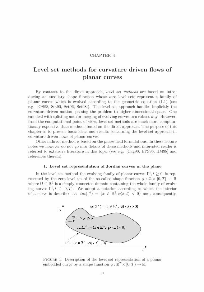
where Ω ⊂ R2 is a simply connected domain containing the whole family of evolv-ing curves Γt, t ∈ [0, T ]. We adopt a notation according to which the interiorof a curve is described as: int(Γt) = x ∈ R2, φ(x, t) < 0 and, consequently,
Figure 1. Description of the level set representation of a planarembedded curve by a shape function φ : R2 × [0, T ) → R.
85
“topicsOnPartialDifferentialEquations” — 2008/1/7 — 16:30 — page 86 — #98
86 4. LEVEL SET METHODS FOR CURVATURE DRIVEN FLOWS OF PLANAR CURVES
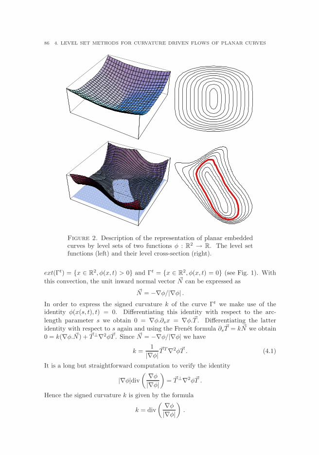
Figure 2. Description of the representation of planar embeddedcurves by level sets of two functions φ : R2 → R. The level setfunctions (left) and their level cross-section (right).
ext(Γt) = x ∈ R2, φ(x, t) > 0 and Γt = x ∈ R2, φ(x, t) = 0 (see Fig. 1). With
this convection, the unit inward normal vector ~N can be expressed as
~N = −∇φ/|∇φ| .In order to express the signed curvature k of the curve Γt we make use of theidentity φ(x(s, t), t) = 0. Differentiating this identity with respect to the arc-
length parameter s we obtain 0 = ∇φ.∂sx = ∇φ.~T . Differentiating the latter
identity with respect to s again and using the Frenet formula ∂s~T = k ~N we obtain
0 = k(∇φ. ~N ) + ~T⊥∇2φ~T . Since ~N = −∇φ/|∇φ| we have
k =1
|∇φ|~T T∇2φ~T . (4.1)
It is a long but straightforward computation to verify the identity
|∇φ|div
( ∇φ|∇φ|
)
= ~T⊥∇2φ~T .
Hence the signed curvature k is given by the formula
k = div
( ∇φ|∇φ|
)
.
“topicsOnPartialDifferentialEquations” — 2008/1/7 — 16:30 — page 87 — #99
1. LEVEL SET REPRESENTATION OF JORDAN CURVES IN THE PLANE 87
In other words, the curvature k is just the minus the divergence of the normal
vector ~N = ∇φ/|∇φ|, i.e. k = −div ~N .Let us differentiate the equation φ(x(s, t), t) = 0 with respect to time. We
obtain ∂tφ + ∇φ.∂tx = 0. Since the normal velocity of x is β = ∂tx. ~N and ~N =−∇φ/|∇φ| we obtain
∂tφ = |∇φ|β .Combining the above identities for ∂tφ, ~N, and k we conclude that the geometricequation (1.1) can be reformulated in terms of the evolution of the shape functionφ = φ(x, t) satisfying the following fully nonlinear parabolic equation:
∂tφ = |∇φ|β (div (∇φ/|∇φ|) , x,−∇φ/|∇φ|) , x ∈ Ω, t ∈ (0, T ) . (4.2)
Here we assume that the normal velocity β may depend on the curvature k, theposition vector x and the tangent angle ν expressed through the unit inward normal
vector ~N , i.e. β = β(k, x, ~N ). Since the behavior of the shape function φ in a fardistance from the set of evolving curves Γt, t ∈ [0, T ], does not influence their evo-lution, it is usual in the context of the level set equation to prescribe homogeneousNeumann boundary conditions at the boundary ∂Ω of the computational domainΩ, i.e.
φ(x, t) = 0 for x ∈ ∂Ω . (4.3)
The initial condition for the level set shape function φ can be constructed as asigned distance function measuring the signed distance of a point x ∈ R2 and theinitial curve Γ0, i.e.
φ(x, 0) = dist(x,Γ0) (4.4)
where dist(x,Γ0) is a signed distance function defined as
dist(x,Γ0) = infy∈Γ0
|x− y|, for x ∈ ext(Γ0) ,
dist(x,Γ0) = − infy∈Γ0
|x− y|, for x ∈ int(Γ0) ,
dist(x,Γ0) = 0, for x ∈ Γ0 .
If we assume that the normal velocity of an evolving curve Γt is an affine in the kvariable, i.e.
β = µk + f
where µ = µ(x, ~N) is a coefficient describing dependence of the velocity speed onthe position vector x and the orientation of the curve Γt expressed through the unit
inward normal vector ~N and f = f(x, ~N) is an external forcing term.
∂tφ = µ |∇φ| div
( ∇φ|∇φ|
)
+ f |∇φ|, x ∈ Ω, t ∈ (0, T ) . (4.5)
1.1. A-priori bounds for the total variation of the shape function.In this section we derive an important a-priori bound for the total variation ofthe shape function satisfying the level set equation (4.2). The total variation (orthe W 1,1 Sobolev norm) of the function φ(., t) is defined as
∫
Ω|∇φ(x, t)| dx where

“topicsOnPartialDifferentialEquations” — 2008/1/7 — 16:30 — page 88 — #100
88 4. LEVEL SET METHODS FOR CURVATURE DRIVEN FLOWS OF PLANAR CURVES
Ω ⊂ R2 is a simply connected domain such that int(Γt) ⊂ Ω for any t ∈ [0, T ].Differentiating the total variation of φ(., t) with respect to time we obtain
d
dt
∫
Ω
|∇φ| dx =
∫
Ω
1
|∇φ| (∇φ.∂t∇φ) dx =
∫
Ω
∇φ|∇φ| .∇∂tφdx
= −∫
Ω
div
( ∇φ|∇φ|
)
.∂tφdx = −∫
Ω
kβ|∇φ| dx
and sod
dt
∫
Ω
|∇φ| dx+
∫
Ω
kβ|∇φ| dx = 0 (4.6)
where k is expressed as in (4.1) and β = β (div (∇φ/|∇φ|) , x,−∇φ/|∇φ|). Withhelp of the co-area integration theorem, the identity (4.6) can be viewed as a levelset analogy to the total length equation (2.14).
In the case of the Euclidean curvature driven flow when curves are evolvedin the normal direction by the curvature (i.e. β = k) we have
∫
Ωkβ|∇φ| dx =
∫
Ωk2|∇φ| dx > 0 and this is why
d
dt
∫
Ω
|∇φ| dx < 0 for any t ∈ (0, T ) ,
implying thus the estimate
φ ∈ L∞((0, T ),W 1,1(Ω)) . (4.7)
The same property can be easily proved by using Gronwall’s lemma for a more
general form of the normal velocity when β = µk + f where µ = µ(x, ~N) >
0, f = f(x, ~N) are globally bounded functions. We presented this estimate becausethe same estimates can be proved for the gradient flow in the theory of minimalsurfaces. Notice that the estimate (4.7) is weaker than the L2–energy estimateφ ∈ L∞((0, T ),W 1,2(Ω)) which can be easily shown for nondegenerate parabolicequation of the form ∂tφ = ∆φ, dφ/dn = 0 on ∂Ω, by multiplying the equationwith the test function φ and integrating over the domain Ω.
2. Viscosity solutions to the level set equation
In this section we briefly describe a concept of viscosity solutions to the levelset equation (4.2). We follow the book by Cao (c.f. [Cao03]). For the sake ofsimplicity of notation we shall consider the normal velocity β of the form β = β(k).Hence equation (4.2) has a simplified form
∂tφ = |∇φ|β (div (∇φ/|∇φ|)) . (4.8)
The concept of viscosity solutions has been introduced by Crandall and Lions in[CL83]. It has been generalized to second order PDEs by Jensen [Jen88] (see also[IS95, FS93]). The proof of the existence and uniqueness of a viscosity solution to(4.8) is a consequence of the maximum principle for viscosity solutions (uniquenesspart). Existence part can be proven by the method of sub and supersolutions knownas the so-called Perron’s method.
Following [Cao03] we first explain the basic idea behind the definition of aviscosity solution. We begin with a simple linear parabolic equation
∂tφ = ∆φ . (4.9)
“topicsOnPartialDifferentialEquations” — 2008/1/7 — 16:30 — page 89 — #101
2. VISCOSITY SOLUTIONS TO THE LEVEL SET EQUATION 89
Let ψ be any C2 smooth function such that φ−ψ < 0 except of some point (x, t) inwhich φ(x, t) = ψ(x, t), i.e. (x, t) is a strict local maximum of the function φ − ψ.Clearly, ∇φ(x, t)−∇ψ(x, t) = 0, ∂tφ(x, t)−∂tψ(x, t) = 0, and ∆(φ(x, t)−ψ(x, t)) ≤0. Hence
∂tψ ≤ ∆ψ at (x, t) . (4.10)
We say that φ is a subsolution to (4.9) if the inequality (4.10) hold whenever φ−ψhas a strict maximum at (x, t). Analogously, we say that φ is a supersolution to(4.9) if the reverse inequality ∂tψ ≥ ∆ψ holds at a point (x, t) in which the functionφ − ψ attains a strict minimum. It is important to realize, that such a definitionof a sub and supersolution does not explicitly require smoothness of the functionφ. It has been introduced by Crandall and Lions in [CL83]. Moreover, the aboveconcept of sub and supersolutions can be extended to the case when the secondorder differential operator contains discontinuities. For the Euclidean motion bymean curvature (i.e. β(k) = k) the existence and uniqueness of a viscosity solutionto (4.8) has been established by Evans and Spruck [ES91] and by Chen, Giga andGoto [CGG91] for the case β(k) is sublinear at ±∞. Finally, Barles, Souganidis andIshii introduced a concept of a viscosity solution for (4.8) in the case of arbitrarycontinuous and nondecreasing function β(k) and they also proved the existence anduniqueness of a viscosity solution in [IS95, BS91]. Moreover, Souganidis extendeda notion of a viscosity solution for the case when the elliptic operator is undefinedin a set of critical points of φ.
Following Souganidis et al. (c.f. [IS95, BS91]), the class A(β) of admissible testfunctions consists of those C2 compactly supported functions ψ : R2 × [0,∞) → R
having the property: if (x, t) is a critical point of ψ, i.e. ∇ψ(x, t) = 0 then thereexists a neighborhood Bδ(x, t) with a radius δ > 0, a function f ∈ F(β), andω ∈ C((0,∞)) satisfying limr→0 ω(r)/r = 0 such that
|ψ(y, s)−ψ(x, t)−∂tψ(x, t)(s−t)| ≤ f(|y−x|)+ω(|s−t|), for any (y, s) ∈ Bδ(x, t) .
The class F(β) consists of those C2 functions f such that f(0) = f ′(0) = f ′′(0) =0, f ′′(r) > 0 for r > 0 and limr→0 f
′(|r|)β(1/r) = 0.The idea behind a relatively complicated definition of the set of admissible
function is simple. It consists in the requirement that test functions must be enoughflat to absorb singularities of the function β at their critical points. With thisconcept of the set of admissible test functions we are in a position to introduce anotion of a viscosity sub and super solution to the level set equation (4.8).
Definition 4.1. [Cao03, Definition 4.3.2] We say that a bounded functionφ : R2 × R → R is a viscosity subsolution to (4.8) if for all admissible functionsψ ∈ A(β), if φ∗ − ψ admits a strict maximum at a point (x, t) then
∂tψ(x, t) ≤ |∇ψ(x, t)|β (div (∇ψ(x, t)/|∇ψ(x, t)|)) , if ∇ψ(x, t) 6= 0,
∂tψ(x, t) ≤ 0, if ∇ψ(x, t) = 0 .
We say that a bounded function φ : R2 × R → R is a viscosity supersolution to(4.8) if for all admissible functions ψ ∈ A(β), if φ∗ −ψ admits a strict minimum ata point (x, t) then
∂tψ(x, t) ≥ |∇ψ(x, t)|β (div (∇ψ(x, t)/|∇ψ(x, t)|)) , if ∇ψ(x, t) 6= 0,
∂tψ(x, t) ≥ 0, if ∇ψ(x, t) = 0 .
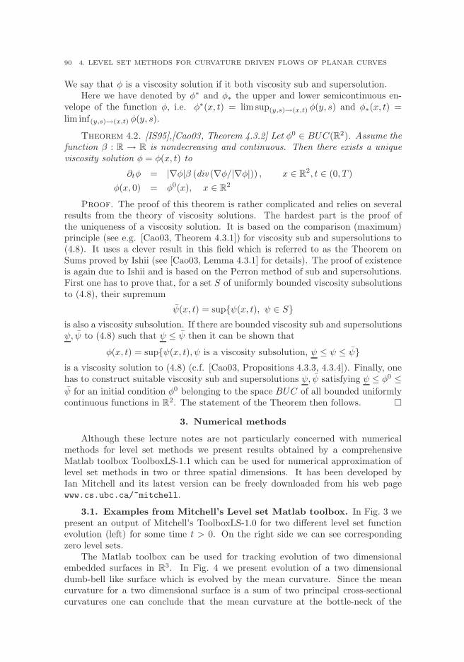
“topicsOnPartialDifferentialEquations” — 2008/1/7 — 16:30 — page 90 — #102
90 4. LEVEL SET METHODS FOR CURVATURE DRIVEN FLOWS OF PLANAR CURVES
We say that φ is a viscosity solution if it both viscosity sub and supersolution.Here we have denoted by φ∗ and φ∗ the upper and lower semicontinuous en-
velope of the function φ, i.e. φ∗(x, t) = lim sup(y,s)→(x,t) φ(y, s) and φ∗(x, t) =
lim inf(y,s)→(x,t) φ(y, s).
Theorem 4.2. [IS95],[Cao03, Theorem 4.3.2] Let φ0 ∈ BUC(R2). Assume thefunction β : R → R is nondecreasing and continuous. Then there exists a uniqueviscosity solution φ = φ(x, t) to
∂tφ = |∇φ|β (div (∇φ/|∇φ|)) , x ∈ R2, t ∈ (0, T )
φ(x, 0) = φ0(x), x ∈ R2
Proof. The proof of this theorem is rather complicated and relies on severalresults from the theory of viscosity solutions. The hardest part is the proof ofthe uniqueness of a viscosity solution. It is based on the comparison (maximum)principle (see e.g. [Cao03, Theorem 4.3.1]) for viscosity sub and supersolutions to(4.8). It uses a clever result in this field which is referred to as the Theorem onSums proved by Ishii (see [Cao03, Lemma 4.3.1] for details). The proof of existenceis again due to Ishii and is based on the Perron method of sub and supersolutions.First one has to prove that, for a set S of uniformly bounded viscosity subsolutionsto (4.8), their supremum
ψ(x, t) = supψ(x, t), ψ ∈ Sis also a viscosity subsolution. If there are bounded viscosity sub and supersolutionsψ, ψ to (4.8) such that ψ ≤ ψ then it can be shown that
φ(x, t) = supψ(x, t), ψ is a viscosity subsolution, ψ ≤ ψ ≤ ψis a viscosity solution to (4.8) (c.f. [Cao03, Propositions 4.3.3, 4.3.4]). Finally, onehas to construct suitable viscosity sub and supersolutions ψ, ψ satisfying ψ ≤ φ0 ≤ψ for an initial condition φ0 belonging to the space BUC of all bounded uniformlycontinuous functions in R2. The statement of the Theorem then follows.
3. Numerical methods
Although these lecture notes are not particularly concerned with numericalmethods for level set methods we present results obtained by a comprehensiveMatlab toolbox ToolboxLS-1.1 which can be used for numerical approximation oflevel set methods in two or three spatial dimensions. It has been developed byIan Mitchell and its latest version can be freely downloaded from his web pagewww.cs.ubc.ca/~mitchell.
3.1. Examples from Mitchell’s Level set Matlab toolbox. In Fig. 3 wepresent an output of Mitchell’s ToolboxLS-1.0 for two different level set functionevolution (left) for some time t > 0. On the right side we can see correspondingzero level sets.
The Matlab toolbox can be used for tracking evolution of two dimensionalembedded surfaces in R3. In Fig. 4 we present evolution of a two dimensionaldumb-bell like surface which is evolved by the mean curvature. Since the meancurvature for a two dimensional surface is a sum of two principal cross-sectionalcurvatures one can conclude that the mean curvature at the bottle-neck of the
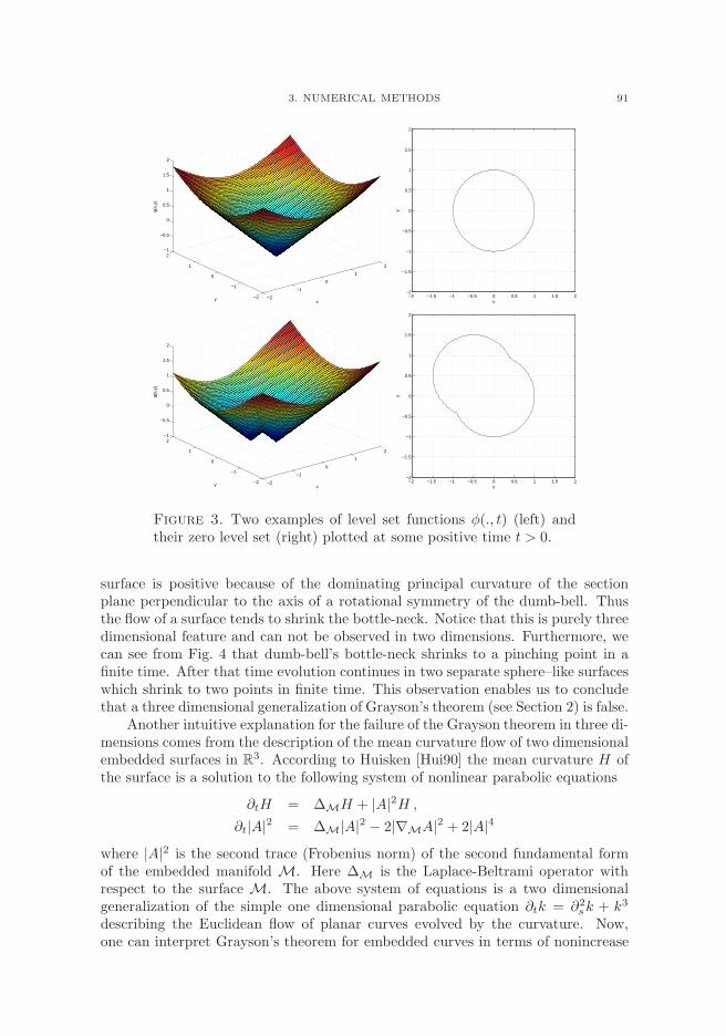
“topicsOnPartialDifferentialEquations” — 2008/1/7 — 16:30 — page 91 — #103
3. NUMERICAL METHODS 91
−2
−1
0
1
2
−2
−1
0
1
2−1
−0.5
0
0.5
1
1.5
2
xy
φ(x,
y)
−2 −1.5 −1 −0.5 0 0.5 1 1.5 2−2
−1.5
−1
−0.5
0
0.5
1
1.5
2
x
y
−2
−1
0
1
2
−2
−1
0
1
2−1
−0.5
0
0.5
1
1.5
2
xy
φ(x,
y)
−2 −1.5 −1 −0.5 0 0.5 1 1.5 2−2
−1.5
−1
−0.5
0
0.5
1
1.5
2
x
y
Figure 3. Two examples of level set functions φ(., t) (left) andtheir zero level set (right) plotted at some positive time t > 0.
surface is positive because of the dominating principal curvature of the sectionplane perpendicular to the axis of a rotational symmetry of the dumb-bell. Thusthe flow of a surface tends to shrink the bottle-neck. Notice that this is purely threedimensional feature and can not be observed in two dimensions. Furthermore, wecan see from Fig. 4 that dumb-bell’s bottle-neck shrinks to a pinching point in afinite time. After that time evolution continues in two separate sphere–like surfaceswhich shrink to two points in finite time. This observation enables us to concludethat a three dimensional generalization of Grayson’s theorem (see Section 2) is false.
Another intuitive explanation for the failure of the Grayson theorem in three di-mensions comes from the description of the mean curvature flow of two dimensionalembedded surfaces in R3. According to Huisken [Hui90] the mean curvature H ofthe surface is a solution to the following system of nonlinear parabolic equations
∂tH = ∆MH + |A|2H ,
∂t|A|2 = ∆M|A|2 − 2|∇MA|2 + 2|A|4
where |A|2 is the second trace (Frobenius norm) of the second fundamental formof the embedded manifold M. Here ∆M is the Laplace-Beltrami operator withrespect to the surface M. The above system of equations is a two dimensionalgeneralization of the simple one dimensional parabolic equation ∂tk = ∂2
sk + k3
describing the Euclidean flow of planar curves evolved by the curvature. Now,one can interpret Grayson’s theorem for embedded curves in terms of nonincrease
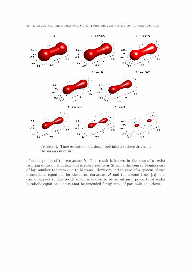
“topicsOnPartialDifferentialEquations” — 2008/1/7 — 16:30 — page 92 — #104
92 4. LEVEL SET METHODS FOR CURVATURE DRIVEN FLOWS OF PLANAR CURVES
Figure 4. Time evolution of a dumb-bell initial surface driven bythe mean curvature.
of nodal points of the curvature k. This result is known in the case of a scalarreaction diffusion equation and is refererred to as Sturm’s theorem or Nonincreaseof lap number theorem due to Matano. However, in the case of a system of twodimensional equations for the mean curvature H and the second trace |A|2 onecannot expect similar result which is known to be an intrinsic property of scalarparabolic equations and cannot be extended for systems of parabolic equations.
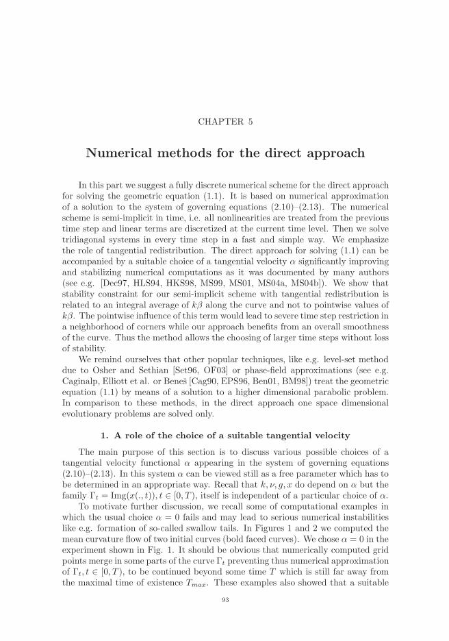
“topicsOnPartialDifferentialEquations” — 2008/1/7 — 16:30 — page 93 — #105
CHAPTER 5
Numerical methods for the direct approach
In this part we suggest a fully discrete numerical scheme for the direct approachfor solving the geometric equation (1.1). It is based on numerical approximationof a solution to the system of governing equations (2.10)–(2.13). The numericalscheme is semi-implicit in time, i.e. all nonlinearities are treated from the previoustime step and linear terms are discretized at the current time level. Then we solvetridiagonal systems in every time step in a fast and simple way. We emphasizethe role of tangential redistribution. The direct approach for solving (1.1) can beaccompanied by a suitable choice of a tangential velocity α significantly improvingand stabilizing numerical computations as it was documented by many authors(see e.g. [Dec97, HLS94, HKS98, MS99, MS01, MS04a, MS04b]). We show thatstability constraint for our semi-implicit scheme with tangential redistribution isrelated to an integral average of kβ along the curve and not to pointwise values ofkβ. The pointwise influence of this term would lead to severe time step restriction ina neighborhood of corners while our approach benefits from an overall smoothnessof the curve. Thus the method allows the choosing of larger time steps without lossof stability.
We remind ourselves that other popular techniques, like e.g. level-set methoddue to Osher and Sethian [Set96, OF03] or phase-field approximations (see e.g.Caginalp, Elliott et al. or Benes [Cag90, EPS96, Ben01, BM98]) treat the geometricequation (1.1) by means of a solution to a higher dimensional parabolic problem.In comparison to these methods, in the direct approach one space dimensionalevolutionary problems are solved only.
1. A role of the choice of a suitable tangential velocity
The main purpose of this section is to discuss various possible choices of atangential velocity functional α appearing in the system of governing equations(2.10)–(2.13). In this system α can be viewed still as a free parameter which has tobe determined in an appropriate way. Recall that k, ν, g, x do depend on α but thefamily Γt = Img(x(., t)), t ∈ [0, T ), itself is independent of a particular choice of α.
To motivate further discussion, we recall some of computational examples inwhich the usual choice α = 0 fails and may lead to serious numerical instabilitieslike e.g. formation of so-called swallow tails. In Figures 1 and 2 we computed themean curvature flow of two initial curves (bold faced curves). We chose α = 0 in theexperiment shown in Fig. 1. It should be obvious that numerically computed gridpoints merge in some parts of the curve Γt preventing thus numerical approximationof Γt, t ∈ [0, T ), to be continued beyond some time T which is still far away fromthe maximal time of existence Tmax. These examples also showed that a suitable
93

“topicsOnPartialDifferentialEquations” — 2008/1/7 — 16:30 — page 94 — #106
94 5. NUMERICAL METHODS FOR THE DIRECT APPROACH
Figure 1. Merging of numerically computed grid points in thecase of the vanishing tangential velocity functional α = 0.
grid points redistribution governed by a nontrivial tangential velocity functional αis needed in order to compute the solution on its maximal time of existence.
The idea behind construction of a suitable tangential velocity functional α israther simple and consists in the analysis of the quantity θ defined as follows:
θ = ln(g/L)
where g = |∂ux| is a local length and L is a total length of a curve Γ = Img(x). Thequantity θ can be viewed as the logarithm of the relative local length g/L. Takinginto account equations (2.12) and (2.14) we have
∂tθ + kβ − 〈kβ〉Γ = ∂sα . (5.1)
By an appropriate choice of ∂sα in the right hand side of (5.1) we can thereforecontrol behavior of θ. Equation (5.1) can be also viewed as a kind of a constitutiverelation determining redistribution of grid points along a curve.
1.1. Non-locally dependent tangential velocity functional. We first an-alyze the case when ∂sα (and so does α) depends on other geometric quantities k, βand g in a nonlocal way. The simplest possible choice of ∂sα is:
∂sα = kβ − 〈kβ〉Γ (5.2)
yielding ∂tθ = 0 in (5.1). Consequently,
g(u, t)
Lt=g(u, 0)
L0for any u ∈ S1, t ∈ [0, Tmax) .
Notice that α can be uniquely computed from (5.2) under the additional renormal-ization constraint: α(0, t) = 0. In the sequel, tangential redistribution driven by asolution α to (5.2) will be refereed to as a parameterization preserving relative locallength. It has been first discovered and utilized by Hou et al. in [HLS94, HKS98]and independently by Mikula and Sevcovic in [MS99, MS01, MS04a, MS04b].
A general choice of α is based on the following setup:
∂sα = kβ − 〈kβ〉Γ +(e−θ − 1
)ω(t) (5.3)
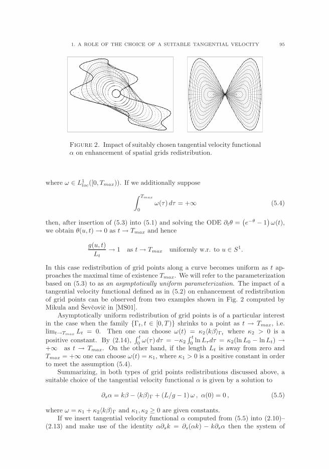
“topicsOnPartialDifferentialEquations” — 2008/1/7 — 16:30 — page 95 — #107
1. A ROLE OF THE CHOICE OF A SUITABLE TANGENTIAL VELOCITY 95
Figure 2. Impact of suitably chosen tangential velocity functionalα on enhancement of spatial grids redistribution.
where ω ∈ L1loc([0, Tmax)). If we additionally suppose
∫ Tmax
0
ω(τ) dτ = +∞ (5.4)
then, after insertion of (5.3) into (5.1) and solving the ODE ∂tθ =(e−θ − 1
)ω(t),
we obtain θ(u, t) → 0 as t→ Tmax and hence
g(u, t)
Lt→ 1 as t→ Tmax uniformly w.r. to u ∈ S1.
In this case redistribution of grid points along a curve becomes uniform as t ap-proaches the maximal time of existence Tmax. We will refer to the parameterizationbased on (5.3) to as an asymptotically uniform parameterization. The impact of atangential velocity functional defined as in (5.2) on enhancement of redistributionof grid points can be observed from two examples shown in Fig. 2 computed byMikula and Sevcovic in [MS01].
Asymptotically uniform redistribution of grid points is of a particular interestin the case when the family Γt, t ∈ [0, T ) shrinks to a point as t → Tmax, i.e.limt→Tmax Lt = 0. Then one can choose ω(t) = κ2〈kβ〉Γt where κ2 > 0 is a
positive constant. By (2.14),∫ t
0 ω(τ) dτ = −κ2
∫ t
0 lnLτdτ = κ2(lnL0 − lnLt) →+∞ as t → Tmax. On the other hand, if the length Lt is away from zero andTmax = +∞ one can choose ω(t) = κ1, where κ1 > 0 is a positive constant in orderto meet the assumption (5.4).
Summarizing, in both types of grid points redistributions discussed above, asuitable choice of the tangential velocity functional α is given by a solution to
∂sα = kβ − 〈kβ〉Γ + (L/g − 1)ω , α(0) = 0 , (5.5)
where ω = κ1 + κ2〈kβ〉Γ and κ1, κ2 ≥ 0 are given constants.If we insert tangential velocity functional α computed from (5.5) into (2.10)–
(2.13) and make use of the identity α∂sk = ∂s(αk) − k∂sα then the system of
“topicsOnPartialDifferentialEquations” — 2008/1/7 — 16:30 — page 96 — #108
96 5. NUMERICAL METHODS FOR THE DIRECT APPROACH
governing equations can be rewritten as follows:
∂tk = ∂2sβ + ∂s(αk) + k〈kβ〉Γ + (1 − L/g)kω , (5.6)
∂tν = β′k∂
2sν + (α+ β′
ν)∂sν + ∇xβ.~T , (5.7)
∂tg = −g〈kβ〉Γ + (L− g)ω , (5.8)
∂tx = β ~N + α~T . (5.9)
It is worth to note that the strong reaction term k2β in (2.10) has been replacedby the averaged term k〈kβ〉Γ in (5.6). A similar phenomenon can be observed in(5.8). This is very important feature as it allows for construction of an efficient andstable numerical scheme.
1.2. Locally dependent tangential velocity functional. Another possi-bility for grid points redistribution along evolved curves is based on a tangentialvelocity functional defined locally. If we take α = ∂sθ, i.e. ∂sα = ∂2
sθ then theconstitutive equation (5.1) reads as follows: ∂tθ + kβ − 〈kβ〉Γ = ∂2
sθ. Since thisequation has a parabolic nature one can expect that variations in θ are decreaingduring evolution and θ tends to a constant value along the curve Γ due to thediffusion process. The advantage of the particular choice
α = ∂sθ = ∂s ln(g/L) = ∂s ln g (5.10)
has been already observed by Deckelnick in [Dec97]. He analyzed the mean curva-ture flow of planar curves (i.e. β = k) by means of a solution to the intrinsic heatequation
∂tx =∂2
ux
|∂ux|2, u ∈ S1, t ∈ (0, T ),
describing evolution of the position vector x of a curve Γt = Img(x(., t)). By using
Frenet’s formulae we obtain ∂tx = k ~N + α~T where α = ∂s ln g = ∂s ln(g/L) = ∂sθ.Inserting the tangential velocity functional α = ∂sθ = ∂s(ln g) into (2.10)–
(2.13) we obtain the following system of governing equations:
∂tk = ∂2sβ + α∂sk + k2β, (5.11)
∂tν = β′k∂
2sν + (α+ β′
ν)∂sν + ∇xβ.~T , (5.12)
∂tg = −gkβ + g∂2s (ln g), (5.13)
∂tx = β ~N + α~T . (5.14)
Notice that equation (5.13) is a nonlinear parabolic equation whereas (5.8) is anonlocal ODE for the local length g.
2. Flowing finite volume approximation scheme
The aim of this part is to review numerical methods for solving the systemof equations (2.10)–(2.13). We begin with a simpler case in which we assume thenormal velocity to be an affine function of the curvature with coefficients dependingon the tangent angle only. Next we consider a slightly generalized form of the normalvelocity in which coefficients may also depend on the position vector x.

“topicsOnPartialDifferentialEquations” — 2008/1/7 — 16:30 — page 97 — #109
2. FLOWING FINITE VOLUME APPROXIMATION SCHEME 97
2.0.1. Normal velocity depending on the tangent angle. First, we consider asimpler case in which the normal velocity β has the following form:
β = β(k, ν) = γ(ν)k + F (5.15)
with a given anisotropy function γ(ν) > 0 and a constant driving force F . Thesystem of governing equations is accompanied by the tangential velocity α given by
∂sα = kβ − 1
L
∫
Γ
kβds− ω(1 − L
g) (5.16)
where L is the total length of the curve Γ and ω is a relaxation function discussedin Section 1.1. Since there is no explicit dependence of flow on spatial position xthe governing equations are simpler and the evolving curve Γt is given (uniquelyup to a translation) by reconstruction
x(u, .) =
∫ u
0
g ~Tdu =
∫ s
0
~Tds. (5.17)
Before performing temporal and spatial discretization we insert (5.16) into (2.10)and (2.12) to obtain
∂tk = ∂2sβ + ∂s(αk) + k〈kβ〉 + kω(1 − L
g), (5.18)
∂tν = β′k∂
2sν + (α+ β′
ν)∂sν , (5.19)
∂tg = −g〈kβ〉 − ω(g − L). (5.20)
From the numerical discretization point of view, critical terms in Eqs. (2.10) –(2.12) are represented by the reaction term k2β in (2.10) and the decay term kβ in(2.12). In Eqs. (5.18) – (5.20) these critical terms were replaced by the averagedvalue of kβ along the curve, thus computation of a local element length in theneighborhood of point with a high curvature is more stable.
In our computational method a solution of the evolution Eq. (1.1) is represented
by discrete plane points xji , i = 0, ..., n, j = 0, ...,m, where index i represents space
discretization and index j a discrete time stepping. Since we only consider closedinitial curves the periodicity condition x0
0 = x0n is required at the beginning. If
we take a uniform division of the time interval [0, T ] with a time step τ = T/mand a uniform division of the fixed parameterization interval [0, 1] with a step
h = 1/n, a point xji corresponds to x(ih, jτ). Difference equations will be given
for discrete quantities kji , ν
ji , rj
i , i = 1, ..., n, j = 1, ...,m representing piecewiseconstant approximations of the curvature, tangent angle and element length for the
segment[
xji−1, x
ji
]
and for αji representing tangential velocity of the flowing node
xj−1i . Then, at the j-th discrete time level, j = 1, ...,m, approximation of a curve
is given by a discrete version of the reconstruction formula (5.17)
xji = xj
0 +
i∑
l=1
rjl (cos(νj
l ), sin(νjl )), i = 1, ..., n. (5.21)
In order to construct a discretization scheme for solving (5.18) – (5.20) we consider
time dependent functions ki(t), νi(t), ri(t), xi(t), αi(t); kji , ν
ji , rj
i , xji , α
ji , described
above, represent their values at time levels t = jτ . Let us denote B = 1L
∫
Γkβds.
“topicsOnPartialDifferentialEquations” — 2008/1/7 — 16:30 — page 98 — #110
98 5. NUMERICAL METHODS FOR THE DIRECT APPROACH
We integrate Eqs. (5.16) and (5.18) – (5.20) at any time t over the so-calledflowing control volume [xi−1, xi]. Using the Newton-Leibniz formula and constantapproximation of the quantities inside flowing control volumes, at any time t weget
αi − αi−1 = rikiβ(ki, νi) − riB − ω
(
ri −L
n
)
.
By taking discrete time stepping, for values of the tangential velocity αji we obtain
αji = αj
i−1 + rj−1i kj−1
i β(kj−1i , νj−1
i ) − rj−1i Bj−1 − ω(rj−1
i −M j−1), (5.22)
i = 1, ..., n, with αj0 = 0 (xj
0 is moving only in the normal direction) where
M j−1 =1
nLj−1, Lj−1 =
n∑
l=1
rj−1l , Bj−1 =
1
Lj−1
n∑
l=1
rj−1l kj−1
l β(kj−1l , νj−1
l )
and ω = κ1 + κ2Bj−1, with input redistribution parameters κ1, κ2. Using similar
approach as above, Eq. (5.20) gives us
dridt
+ riB + riω = ωL
n.
By taking a backward time difference we obtain an update for local lengths
rji =
rj−1i + τωM j−1
1 + τ(Bj−1 + ω), i = 1, ..., n, rj
0 = rjn, rj
n+1 = rj1. (5.23)
Subsequently, new local lengths are used for approximation of intrinsic derivativesin (5.18) – (5.19). Integrating the curvature Eq. (5.18) in flowing control volume[xi−1, xi] we have
ridki
dt= [∂sβ(k, ν)]xi
xi−1+ [αk]xi
xi−1+ ki(ri(B + ω) − ω
L
n).
Now, by replacing the time derivative by time difference, approximating k in nodalpoints by the average value of neighboring segments, and using semi-implicit ap-proach we obtain a tridiagonal system with periodic boundary conditions imposedfor new discrete values of the curvature
ajik
ji−1 + bjik
ji + cjik
ji+1 = dj
i , i = 1, ..., n, kj0 = kj
n, kjn+1 = kj
1, (5.24)
where
aji =
αji−1
2− γ(νj−1
i−1 )
qji−1
, cji = −αji
2− γ(νj−1
i+1 )
qji
, dji =
rji
τkj−1
i ,
bji = rji
(1
τ− (Bj−1 + ω)
)
+ ωM j−1 − αji
2+αj
i−1
2+γ(νj−1
i )
qji−1
+γ(νj−1
i )
qji
where qji =
rji +rj
i+1
2 , i = 1, ..., n. Finally, by integrating the tangent angle Eq.(5.19) we get
ridνi
dt= γ(νi) [∂sν]
xi
xi−1+ [αν]
xi
xi−1− νi(αi − αi−1) + γ′(νi)ki [ν]
xi
xi−1.
Again, values of the tangent angle ν in nodal points are approximated by theaverage of neighboring segments values, the time derivative is replaced by the time

“topicsOnPartialDifferentialEquations” — 2008/1/7 — 16:30 — page 99 — #111
2. FLOWING FINITE VOLUME APPROXIMATION SCHEME 99
difference and using a semi-implicit approach we obtain tridiagonal system withperiodic boundary conditions for new values of the tangent angle
Ajiν
ji−1 +Bj
i νji + Cj
i νji+1 = Dj
i , i = 1, ..., n, νj0 = νj
n, νjn+1 = νj
1 , (5.25)
where
Aji =
αji−1
2+γ′(νj−1
i )kji
2− γ(νj−1
i )
qji−1
, Bji =
rji
τ− (Aj
i + Cji ),
Cji = −α
ji
2− γ′(νj−1
i )kji
2− γ(νj−1
i )
qji
, Dji =
rji
τνj−1
i .
The initial quantities for the algorithm are computed as follows:
Ri = (Ri1 , Ri2) = x0i − x0
i−1, i = 1, ..., n, R0 = Rn, Rn+1 = R1,
r0i = |Ri|, i = 0, ..., n+ 1, (5.26)
k0i = 1
2r0isgn (det(Ri−1, Ri+1)) arccos
(Ri+1.Ri−1
r0i+1r0
i−1
)
, (5.27)
i = 1, ..., n, k00 = k0
n, k0n+1 = k0
1 ,
ν00 = arccos(Ri1/r
0i ) if Ri2 ≥ 0, ν0
0 = 2π − arccos(Ri1/ri) if Ri2 < 0,
ν0i = ν0
i−1 + r0i k0i , i = 1, ..., n+ 1. (5.28)
Remark (Solvability and stability of the scheme.) Let us first examine discretevalues of the tangent angle ν computed from (5.25). One can rewrite it into theform
νji +
τ
rji
Cji (νj
i+1 − νji ) +
τ
rji
Aji (ν
ji−1 − νj
i ) = νj−1i . (5.29)
Let maxk
νjk be attained at the i-th node. We can always take a fine enough resolution
of the curve, i.e. take small qji ≪ 1, i = 1, .., n, such that both Aj
i and Cji are
nonpositive and thus the second and third terms on the left hand side of (5.29) are
nonnegative. Then maxk
νjk = νj
i ≤ νj−1i ≤ max
kνj−1
k . By a similar argument we can
derive an inequality for the minimum. In this way we have shown the L∞-stabilitycriterion, namely
minkν0
k ≤ minkνj
k ≤ maxk
νjk ≤ max
kν0
k , j = 1, ..,m.
Notice that in the continuous case the above comparison inequality is a consequence
of the parabolic maximum principle for equation (5.7) in which the term ∇xβ.~T isvanishing as β does not explicitly depend on the position vector x.
Having guaranteed non-positivity of Aji and Cj
i we can conclude positivity and
diagonal dominance of the diagonal term Bji . In particular, it implies that the
tridiagonal matrix of the system (5.25) is an M -matrix and hence a solution to(5.25) always exists and is unique.
In the same way, by taking qji small enough, we can prove nonpositivity of
the off-diagonal terms aji and cji in the system (5.24) for discrete curvature values.
Then the diagonal term bji is positive and dominant provided that τ(Bj−1 +ω) < 1.Again we have shown that the corresponding matrix is an M -matrix and thereforethere exists a unique solution to the system (5.24).
“topicsOnPartialDifferentialEquations” — 2008/1/7 — 16:30 — page 100 — #112
100 5. NUMERICAL METHODS FOR THE DIRECT APPROACH
Another natural stability requirement of the scheme is related to the positivityof local lengths rj
i during computations. It follows from (5.23) that the positivity
of rji is equivalent to the condition τ(Bj−1 + ω) > −1. Taking into account both
inequalities for the time step we end up with the following stability restriction onthe time step τ :
τ ≤ 1
|Bj−1 + ω| (5.30)
related to Bj−1 (a discrete average value of kβ over a curve).
2.0.2. Normal velocity depending on the tangent angle and the position vector.Next we consider a more general motion of the curves with explicit dependenceof the flow on position x and suggest numerical scheme for such a situation. Weconsider (1.1) with a linear dependence of β on the curvature, i.e.
β(k, x, ν) = δ(x, ν)k + c(x, ν)
where δ(x, ν) > 0. By using Frenet’s formulae one can rewrite the position vectorEq. (2.13) as an intrinsic convection-diffusion equation for the vector x and we getthe system
∂tk = ∂2sβ + ∂s(αk) + k
1
L
∫
Γ
kβds+ kω(1 − L
g) , (5.31)
∂tν = β′k∂
2sν + (α+ β′
ν)∂sν + ∇xβ.~T , (5.32)
∂tg = −g 1
L
∫
Γ
kβds− ω(g − L) , (5.33)
∂tx = δ(x, ν)∂2sx+ α∂sx+ ~c(x, ν) , (5.34)
where ~c(x, ν) = c(x, ν) ~N = (−c(x, ν) sin ν, c(x, ν) cos ν). In comparison to thescheme given above, two new tridiagonal systems have to be solved at each timelevel in order to update the curve position vector x. The curve position itself andall geometric quantities entering the model are resolved from their own intrinsicEqs. (5.31) – (5.34). In order to construct a discretization scheme, Eqs. (5.31) –(5.33) together with (5.16) are integrated over a flowing control volume [xi−1, xi].
We also construct a time dependent dual volumes[
xji−1, x
ji
]
, i = 1, .., n, j = 1, ..,m,
where xji =
xji−1+xj
i
2 over which the last Eq. (5.34) will be integrated. Then, forvalues of the tangential velocity we obtain
αji = αj
i−1 + rj−1i kj−1
i β(xj−1i , kj−1
i , νj−1i ) − rj−1
i Bj−1 − ω(rj−1i −M j−1),
i = 1, ..., n, αj0 = 0, (5.35)
with M j−1, Lj−1, ω given as above and
Bj−1 =1
Lj−1
n∑
l=1
rj−1l kj−1
l β(xj−1l , kj−1
l , νj−1l ).
Local lengths are updated by the formula:
rji =
rj−1i + τωM j−1
1 + τ(Bj−1 + ω), i = 1, ..., n, rj
0 = rjn, rj
n+1 = rj1. (5.36)
“topicsOnPartialDifferentialEquations” — 2008/1/7 — 16:30 — page 101 — #113
2. FLOWING FINITE VOLUME APPROXIMATION SCHEME 101
The tridiagonal system for discrete values of the curvature reads as follows:
ajik
ji−1 + bjik
ji + cjik
ji+1 = dj
i , i = 1, ..., n, kj0 = kj
n, kjn+1 = kj
1, (5.37)
where
aji =
αji−1
2− δ(xj−1
i−1 , νj−1i−1 )
qji−1
, cji = −αji
2− δ(xj−1
i+1 , νj−1i+1 )
qji
,
bji = rji
(1
τ− (Bj−1 + ω)
)
+ ωM j−1 − αji
2+αj
i−1
2+δ(xj−1
i , νj−1i )
qji−1
+δ(xj−1
i , νj−1i )
qji
,
dji =
rji
τkj−1
i +c(xj−1
i+1 , νj−1i+1 ) − c(xj−1
i , νj−1i )
qji
− c(xj−1i , νj−1
i ) − c(xj−1i−1 , ν
j−1i−1 )
qji−1
.
The tridiagonal system for new values of the tangent angle is given by
Ajiν
ji−1 +Bj
i νji + Cj
i νji+1 = Dj
i , i = 1, ..., n, νj0 = νj
n, νjn+1 = νj
1 , (5.38)
where
Aji =
αji−1 + β′
ν(xj−1i , kj
i , νj−1i )
2− δ(xj−1
i , νj−1i )
qji−1
,
Cji = −α
ji + β′
ν(xj−1i , kj
i , νj−1i )
2− δ(xj−1
i , νj−1i )
qji
,
Bji =
rji
τ− (Aj
i + Cji ), Dj
i =rji
τνj−1
i + rji∇xβ(xj−1
i , νj−1i , kj
i ).(cos(νj−1i ), sin(νj−1
i )).
Finally, we end up with two tridiagonal systems for updating the position vector
Ajix
ji−1 + Bj
ixji + Cj
i xji+1 = Dj
i , i = 1, ..., n, xj0 = xj
n, xjn+1 = xj
1, (5.39)
where
Aji = −δ(x
j−1i , 1
2 (νji + νj
i+1))
rji
+αj
i
2, Cj
i = −δ(xj−1i , 1
2 (νji + νj
i+1))
rji+1
− αji
2,
Bji =
qji
τ− (Aj
i + Cji ), Dj
i =qji
τxj−1
i + qji~c(x
j−1i ,
1
2(νj
i + νji+1)).
The initial quantities for the algorithm are given by (5.26) – (5.28).

“topicsOnPartialDifferentialEquations” — 2008/1/7 — 16:30 — page 102 — #114
“topicsOnPartialDifferentialEquations” — 2008/1/7 — 16:30 — page 103 — #115
CHAPTER 6
Applications of curvature driven flows
1. Computation of curvature driven evolution of planar curves withexternal force
In following figures we present numerical solutions computed by the scheme;initial curves are plotted with a thick line and the numerical solution is given byfurther solid lines with points representing the motion of some grid points dur-ing the curve evolution. In Figure 1 we compare computations with and withouttangential redistribution for a large driving force F . As an initial curve we chosex1(u) = cos(2πu), x2(u) = 2 sin(2πu) − 1.99 sin3(2πu), u ∈ [0, 1]. Without re-distribution, the computations are collapsing soon because of the degeneracy inlocal element lengths in parts of a curve with high curvature leading to a merg-ing of the corresponding grid points. Using the redistribution the evolution canbe successfully handled. We used τ = 0.00001, 400 discrete grid points and weplotted every 150th time step. In Figure 2 we have considered an initial curvex1(u) = (1 − C cos2(2πu)) cos(2πu), x2(u) = (1 − C cos2(2πu)) sin(2πu), u ∈ [0, 1]with C = 0.7. We took τ = 0.00001 and 800 (Figure 2 left) and 1600 (Figure 2right) grid points for representation of a curve. In Figure 2 left we plot each 500thtime step, and in Figure 2 right each 100th step. It is natural that we have touse small time steps in case of strong driving force. However, the time step is notrestricted by the point-wise values of the almost singular curvature in the cornerswhich would lead to an un-realistic time step restriction. According to (5.30), thetime step is restricted by the average value of kβ computed over the curve whichis much more weaker restriction because of the regularity of the curve outside thecorners. In Figure 3 we present experiments with three-fold anisotropy startingwith unit circle. We used τ = 0.001, 300 grid points and we plotted every 50thtime step (left) and every 750th time step (right). In all experiments we choseredistribution parameters κ1 = κ2 = 10.
2. Flows of curves on a surface driven by the geodesic curvature
The purpose of this section is to analytically and numerically investigate a flowof closed curves on a given graph surface driven by the geodesic curvature. Weshow how such a flow can be reduced to a flow of vertically projected planar curvesgoverned by a solution of a fully nonlinear system of parabolic differential equations.We present various computational examples of evolution of surface curves drivenby the geodesic curvature are presented in this part. The normal velocity V of theevolving family of surface curves Gt, t ≥ 0, is proportional to the geodesic curvature
103

“topicsOnPartialDifferentialEquations” — 2008/1/7 — 16:30 — page 104 — #116
104 6. APPLICATIONS OF CURVATURE DRIVEN FLOWS
Figure 1. Isotropic curvature driven motion, β(k, ν) = εk + F ,with ε = 1, F = 10, without (left) and with (right) uniform tan-gential redistribution of grid points.
Figure 2. Isotropic curvature driven motion of an initial non-convex curve including uniform tangential redistribution of gridpoints; β(k, ν) = εk + F , with ε = 1, F = −10 (left) and ε = 0.1,F = −10 (right). Resolution of sharp corners in the case of a highlydominant forcing term using the algorithm with redistribution ispossible.
Kg of Gt, i.e.V = δKg (6.1)
where δ = δ(X, ~N ) > 0 is a smooth positive coefficient describing anisotropy de-
pending on the position X and the orientation of the unit inward normal vector ~Nto the curve on a surface.
The idea how to analyze and compute numerically such a flow is based on theso-called direct approach method applied to a flow of vertically projected family ofplanar curves. Vertical projection of surface curves on a simple surface M into theplane R2. It allows for reducing the problem to the analysis of evolution of planar
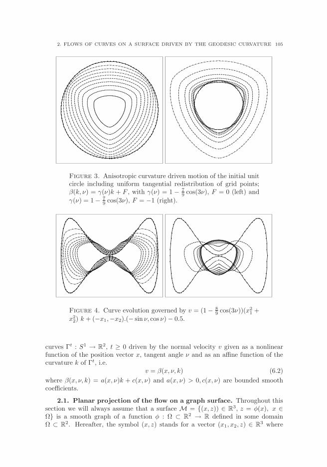
“topicsOnPartialDifferentialEquations” — 2008/1/7 — 16:30 — page 105 — #117
2. FLOWS OF CURVES ON A SURFACE DRIVEN BY THE GEODESIC CURVATURE 105
Figure 3. Anisotropic curvature driven motion of the initial unitcircle including uniform tangential redistribution of grid points;β(k, ν) = γ(ν)k + F , with γ(ν) = 1 − 7
9 cos(3ν), F = 0 (left) and
γ(ν) = 1 − 79 cos(3ν), F = −1 (right).
Figure 4. Curve evolution governed by v = (1 − 89 cos(3ν))(x2
1 +
x22) k + (−x1,−x2).(− sin ν, cos ν) − 0.5.
curves Γt : S1 → R2, t ≥ 0 driven by the normal velocity v given as a nonlinear
function of the position vector x, tangent angle ν and as an affine function of thecurvature k of Γt, i.e.
v = β(x, ν, k) (6.2)
where β(x, ν, k) = a(x, ν)k + c(x, ν) and a(x, ν) > 0, c(x, ν) are bounded smoothcoefficients.
2.1. Planar projection of the flow on a graph surface. Throughout thissection we will always assume that a surface M = (x, z)) ∈ R3, z = φ(x), x ∈Ω is a smooth graph of a function φ : Ω ⊂ R2 → R defined in some domainΩ ⊂ R2. Hereafter, the symbol (x, z) stands for a vector (x1, x2, z) ∈ R3 where

“topicsOnPartialDifferentialEquations” — 2008/1/7 — 16:30 — page 106 — #118
106 6. APPLICATIONS OF CURVATURE DRIVEN FLOWS
x = (x1, x2) ∈ R2. In such a case any smooth closed curve G on the surface Mcan be then represented by its vertical projection to the plane, i.e. G = (x, z) ∈R
3, x ∈ Γ, z = φ(x) where Γ is a closed planar curve in R2. Recall, that for a curve
G = (x, φ(x)) ∈ R3, x ∈ Γ on a surface M = (x1, x2, φ(x1, x2)) ∈ R3, (x1, x2) ∈Ω the geodesic curvature Kg is given by
Kg =−√
EG− F 2
(
x′′1x′2 − x′1x
′′2 − Γ2
11x′31 + Γ1
22x′32
−(2Γ212 − Γ1
11)x′21 x
′2 + (2Γ1
12 − Γ222)x
′1x
′22
)
where E,G, F are coefficients of the first fundamental form and Γkij are Christoffel
symbols of the second kind. Here (.)′ denotes the derivative with respect to the unitspeed parameterization of a curve on a surface. In terms of geometric quantitiesrelated to a vertically projected planar curve we obtain, after some calculations,that
Kg =1
(
1 + (∇φ.~T )2) 3
2
(
(1 + |∇φ|2
) 12 k +
~T T∇2φ ~T
(1 + |∇φ|2) 12
∇φ. ~N)
(6.3)
(see [MS04b]). Moreover, the unit inward normal vector ~N ⊥ Tx(M) to a surfacecurve G ⊂ M relative to M can be expressed as
~N =
(
(1 + (∇φ.~T )2) ~N − (∇φ.~T )(∇φ. ~N )~T , ∇φ. ~N)
(
(1 + |∇φ|2)(1 + (∇φ.~T )2)) 1
2
(see also [MS04b]). Hence for the normal velocity V of Gt = (x, φ(x)), x ∈ Γt wehave
V = ∂t(x, φ(x)). ~N = ( ~N,∇φ. ~N).β ~N =
(
1 + |∇φ|21 + (∇φ.~T )2
) 12
β
where β is the normal velocity of the vertically projected planar curve Γt having the
unit inward normal ~N and tangent vector ~T . Following the so-called direct approach(see [Dec97, Dzi94, Dzi99, HLS94, Mik97, MS99, MS01, MS04a, MS04b, MS06]) theevolution of planar curves Γt, t ≥ 0, can be described by a solution x = x(., t) ∈ R2
to the position vector equation ∂tx = β ~N + α~T where β and α are normal andtangential velocities of Γt, resp. Assuming the family of surface curves Gt satisfies(6.1) it has been shown in [MS04b] that the geometric equation v = β(x, k, ν) forthe normal velocity v of the vertically projected planar curve Γt can be written inthe following form:
v = β(x, k, ν) ≡ a(x, ν) k − b(x, ν)∇φ(x). ~N (6.4)
where a = a(x, ν) > 0 and b = b(x, ν) are smooth functions given by
a(x, ν) =δ
1 + (∇φ.~T )2, b(x, ν) = −a(x, ν)
~T T∇2φ ~T
1 + |∇φ|2 , (6.5)
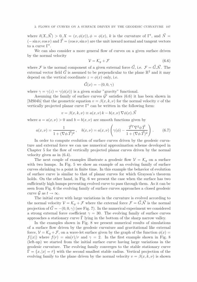
“topicsOnPartialDifferentialEquations” — 2008/1/7 — 16:30 — page 107 — #119
2. FLOWS OF CURVES ON A SURFACE DRIVEN BY THE GEODESIC CURVATURE 107
where δ(X, ~N ) > 0, X = (x, φ(x)), φ = φ(x), k is the curvature of Γt, and ~N =
(− sin ν, cos ν) and ~T = (cos ν, sin ν) are the unit inward normal and tangent vectorsto a curve Γt.
We can also consider a more general flow of curves on a given surface drivenby the normal velocity
V = Kg + F (6.6)
where F is the normal component of a given external force ~G, i.e. F = ~G. ~N . The
external vector field ~G is assumed to be perpendicular to the plane R2 and it maydepend on the vertical coordinate z = φ(x) only, i.e.
~G(x) = −(0, 0, γ)
where γ = γ(z) = γ(φ(x)) is a given scalar ”gravity” functional.Assuming the family of surface curves Gt satisfies (6.6) it has been shown in
[MS04b] that the geometric equation v = β(x, k, ν) for the normal velocity v of thevertically projected planar curve Γt can be written in the following form:
v = β(x, k, ν) ≡ a(x, ν) k − b(x, ν)∇φ(x). ~N
where a = a(x, ν) > 0 and b = b(x, ν) are smooth functions given by
a(x, ν) =1
1 + (∇φ.~T )2, b(x, ν) = a(x, ν)
(
γ(φ) −~T T∇2φ ~T
1 + (∇φ.~T )2
)
. (6.7)
In order to compute evolution of surface curves driven by the geodesic curva-ture and external force we can use numerical approximation scheme developed inChapter 5 for the flow of vertically projected planar curves driven by the normalvelocity given as in (6.4).
The next couple of examples illustrate a geodesic flow V = Kg on a surfacewith two humps. In Fig. 5 we show an example of an evolving family of surfacecurves shrinking to a point in finite time. In this example the behavior of evolutionof surface curve is similar to that of planar curves for which Grayson’s theoremholds. On the other hand, in Fig. 6 we present the case when the surface has twosufficiently high humps preventing evolved curve to pass through them. As it can beseen from Fig. 6 the evolving family of surface curves approaches a closed geodesiccurve G as t → ∞.
The initial curve with large variations in the curvature is evolved according to
the normal velocity V = Kg + F where the external force F = ~G. ~N is the normal
projection of ~G = −(0, 0, γ) (see Fig. 7). In the numerical experiment we considereda strong external force coefficient γ = 30. The evolving family of surface curvesapproaches a stationary curve Γ lying in the bottom of the sharp narrow valley.
In the examples shown in Fig. 8 we present numerical results of simulationsof a surface flow driven by the geodesic curvature and gravitational like externalforce, V = Kg +F , on a wave-let surface given by the graph of the function φ(x) =f(|x|) where f(r) = sin(r)/r and γ = 2. In the first example shown in Fig. 8(left-up) we started from the initial surface curve having large variations in thegeodesic curvature. The evolving family converges to the stable stationary curveΓ = x, |x| = r with the second smallest stable radius. Vertical projection of theevolving family to the plane driven by the normal velocity v = β(x, k, ν) is shown
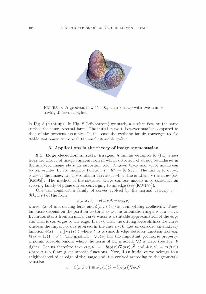
“topicsOnPartialDifferentialEquations” — 2008/1/7 — 16:30 — page 108 — #120
108 6. APPLICATIONS OF CURVATURE DRIVEN FLOWS
Figure 5. A geodesic flow V = Kg on a surface with two humpshaving different heights.
in Fig. 8 (right-up). In Fig. 8 (left-bottom) we study a surface flow on the samesurface the same external force. The initial curve is however smaller compared tothat of the previous example. In this case the evolving family converges to thestable stationary curve with the smallest stable radius.
3. Applications in the theory of image segmentation
3.1. Edge detection in static images. A similar equation to (1.1) arisesfrom the theory of image segmentation in which detection of object boundaries inthe analyzed image plays an important role. A given black and white image canbe represented by its intensity function I : R2 → [0, 255]. The aim is to detectedges of the image, i.e. closed planar curves on which the gradient ∇I is large (see[KM95]). The method of the so-called active contour models is to construct anevolving family of plane curves converging to an edge (see [KWT87]).
One can construct a family of curves evolved by the normal velocity v =β(k, x, ν) of the form
β(k, x, ν) = δ(x, ν)k + c(x, ν)
where c(x, ν) is a driving force and δ(x, ν) > 0 is a smoothing coefficient. Thesefunctions depend on the position vector x as well as orientation angle ν of a curve.Evolution starts from an initial curve whcih is a suitable approximation of the edgeand then it converges to the edge. If c > 0 then the driving force shrinks the curvewhereas the impact of c is reversed in the case c < 0. Let us consider an auxiliaryfunction φ(x) = h(|∇I(x)|) where h is a smooth edge detector function like e.g.h(s) = 1/(1 + s2). The gradient −∇φ(x) has the important geometric property:it points towards regions where the norm of the gradient ∇I is large (see Fig. 9
right). Let us therefore take c(x, ν) = −b(φ(x))∇φ(x). ~N and δ(x, ν) = a(φ(x))where a, b > 0 are given smooth functions. Now, if an initial curve belongs to aneighborhood of an edge of the image and it is evolved according to the geometricequation
v = β(x, k, ν) ≡ a(φ(x))k − b(φ(x))∇φ. ~N
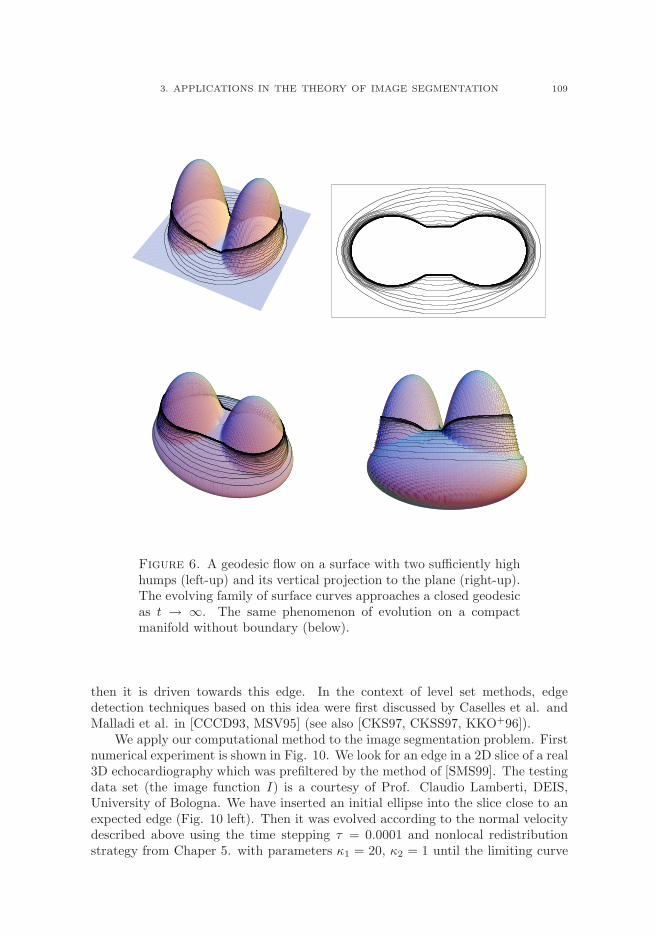
“topicsOnPartialDifferentialEquations” — 2008/1/7 — 16:30 — page 109 — #121
3. APPLICATIONS IN THE THEORY OF IMAGE SEGMENTATION 109
Figure 6. A geodesic flow on a surface with two sufficiently highhumps (left-up) and its vertical projection to the plane (right-up).The evolving family of surface curves approaches a closed geodesicas t → ∞. The same phenomenon of evolution on a compactmanifold without boundary (below).
then it is driven towards this edge. In the context of level set methods, edgedetection techniques based on this idea were first discussed by Caselles et al. andMalladi et al. in [CCCD93, MSV95] (see also [CKS97, CKSS97, KKO+96]).
We apply our computational method to the image segmentation problem. Firstnumerical experiment is shown in Fig. 10. We look for an edge in a 2D slice of a real3D echocardiography which was prefiltered by the method of [SMS99]. The testingdata set (the image function I) is a courtesy of Prof. Claudio Lamberti, DEIS,University of Bologna. We have inserted an initial ellipse into the slice close to anexpected edge (Fig. 10 left). Then it was evolved according to the normal velocitydescribed above using the time stepping τ = 0.0001 and nonlocal redistributionstrategy from Chaper 5. with parameters κ1 = 20, κ2 = 1 until the limiting curve
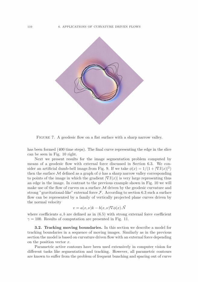
“topicsOnPartialDifferentialEquations” — 2008/1/7 — 16:30 — page 110 — #122
110 6. APPLICATIONS OF CURVATURE DRIVEN FLOWS
Figure 7. A geodesic flow on a flat surface with a sharp narrow valley.
has been formed (400 time steps). The final curve representing the edge in the slicecan be seen in Fig. 10 right.
Next we present results for the image segmentation problem computed bymeans of a geodesic flow with external force discussed in Section 6.3. We con-sider an artificial dumb-bell image.from Fig. 9. If we take φ(x) = 1/(1 + |∇I(x)|2)then the surface M defined as a graph of φ has a sharp narrow valley correspondingto points of the image in which the gradient |∇I(x)| is very large representing thusan edge in the image. In contrast to the previous example shown in Fig. 10 we willmake use of the flow of curves on a surface M driven by the geodesic curvature andstrong ”gravitational-like” external force F . According to section 6.3 such a surfaceflow can be represented by a family of vertically projected plane curves driven bythe normal velocity
v = a(x, ν)k − b(x, ν)∇φ(x). ~N
where coefficients a, b are defined as in (6.5) with strong external force coefficientγ = 100. Results of computation are presented in Fig. 11.
3.2. Tracking moving boundaries. In this section we describe a model fortracking boundaries in a sequence of moving images. Similarly as in the previoussection the model is based on curvature driven flow with an external force dependingon the position vector x.
Parametric active contours have been used extensively in computer vision fordifferent tasks like segmentation and tracking. However, all parametric contoursare known to suffer from the problem of frequent bunching and spacing out of curve
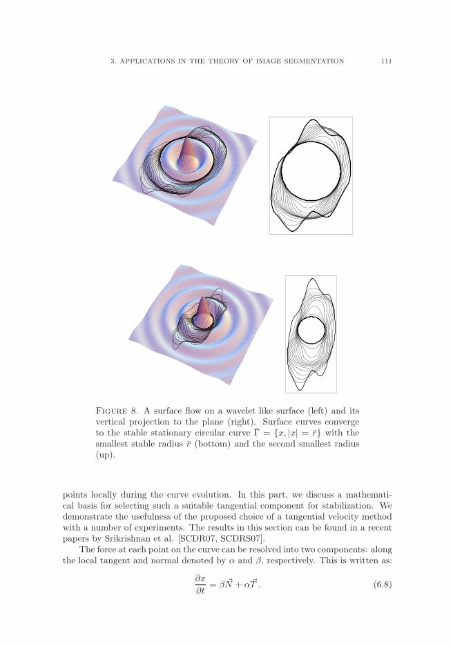
“topicsOnPartialDifferentialEquations” — 2008/1/7 — 16:30 — page 111 — #123
3. APPLICATIONS IN THE THEORY OF IMAGE SEGMENTATION 111
Figure 8. A surface flow on a wavelet like surface (left) and itsvertical projection to the plane (right). Surface curves convergeto the stable stationary circular curve Γ = x, |x| = r with thesmallest stable radius r (bottom) and the second smallest radius(up).
points locally during the curve evolution. In this part, we discuss a mathemati-cal basis for selecting such a suitable tangential component for stabilization. Wedemonstrate the usefulness of the proposed choice of a tangential velocity methodwith a number of experiments. The results in this section can be found in a recentpapers by Srikrishnan et al. [SCDR07, SCDRS07].
The force at each point on the curve can be resolved into two components: alongthe local tangent and normal denoted by α and β, respectively. This is written as:
∂x
∂t= β ~N + α~T . (6.8)
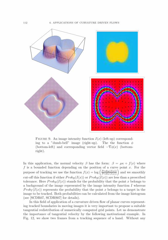
“topicsOnPartialDifferentialEquations” — 2008/1/7 — 16:30 — page 112 — #124
112 6. APPLICATIONS OF CURVATURE DRIVEN FLOWS
Figure 9. An image intensity function I(x) (left-up) correspond-ing to a ”dumb-bell” image (right-up). The the function φ(bottom-left) and corresponding vector field −∇φ(x) (bottom-right).
In this application, the normal velocity β has the form: β = µκ + f(x) wheref is a bounded function depending on the position of a curve point x. For the
purpose of tracking we use the function f(x) = log(
ProbB(I(x))ProbT (I(x))
)
and we smoothly
cut-off this function if either ProbB(I(x)) or ProbB(I(x)) are less than a prescribedtolerance. Here ProbB(I(x)) stands for the probability that the point x belongs toa background of the image represented by the image intensity function I whereasProbT (I(x)) represents the probability that the point x belongs to a target in theimage to be tracked. Both probabilities can be calculated from the image histogram(see [SCDR07, SCDRS07] for details).
In this field of application of a curvature driven flow of planar curves represent-ing tracked boundaries in moving images it is very important to propose a suitabletangential redistribution of numerically computed grid points. Let us demonstratethe importance of tangential velocity by the following motivational example. InFig. 12, we show two frames from a tracking sequence of a hand. Without any
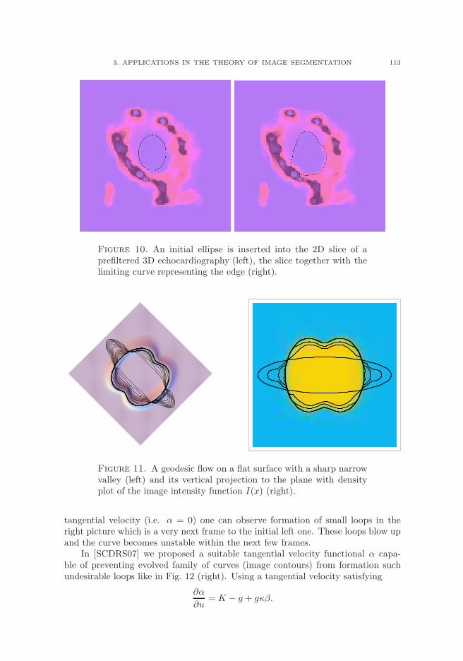
“topicsOnPartialDifferentialEquations” — 2008/1/7 — 16:30 — page 113 — #125
3. APPLICATIONS IN THE THEORY OF IMAGE SEGMENTATION 113
Figure 10. An initial ellipse is inserted into the 2D slice of aprefiltered 3D echocardiography (left), the slice together with thelimiting curve representing the edge (right).
Figure 11. A geodesic flow on a flat surface with a sharp narrowvalley (left) and its vertical projection to the plane with densityplot of the image intensity function I(x) (right).
tangential velocity (i.e. α = 0) one can observe formation of small loops in theright picture which is a very next frame to the initial left one. These loops blow upand the curve becomes unstable within the next few frames.
In [SCDRS07] we proposed a suitable tangential velocity functional α capa-ble of preventing evolved family of curves (image contours) from formation suchundesirable loops like in Fig. 12 (right). Using a tangential velocity satisfying
∂α
∂u= K − g + gκβ.
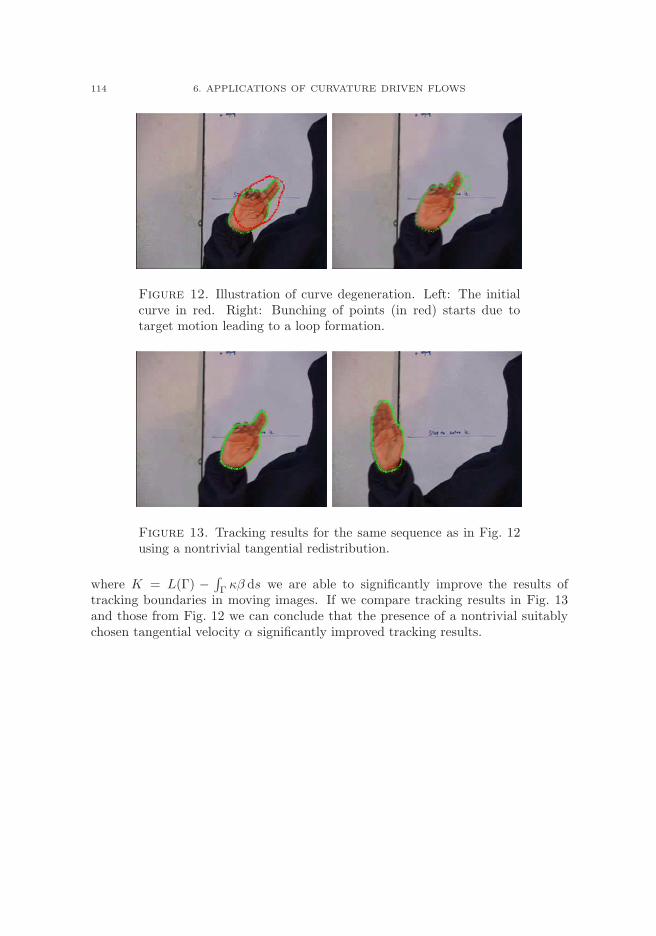
“topicsOnPartialDifferentialEquations” — 2008/1/7 — 16:30 — page 114 — #126
114 6. APPLICATIONS OF CURVATURE DRIVEN FLOWS
Figure 12. Illustration of curve degeneration. Left: The initialcurve in red. Right: Bunching of points (in red) starts due totarget motion leading to a loop formation.
Figure 13. Tracking results for the same sequence as in Fig. 12using a nontrivial tangential redistribution.
where K = L(Γ) −∫
Γ κβ ds we are able to significantly improve the results oftracking boundaries in moving images. If we compare tracking results in Fig. 13and those from Fig. 12 we can conclude that the presence of a nontrivial suitablychosen tangential velocity α significantly improved tracking results.

“topicsOnPartialDifferentialEquations” — 2008/1/7 — 16:30 — page 115 — #127
Bibliography
[AG89] S. Angenent and M. E. Gurtin, Multiphase thermomechanics with inter-facial structure. II: Evolution of an isothermal interface, Arch. Ration.Mech. Anal. 108 (1989), no. 4, 323–391.
[AG94] S. Angenent and M. Gurtin, Anisotropic motion of a phase interface.Well-posedness of the initial value problem and qualitative propertiesof the interface, J. Reine Angew. Math. 446 (1994), 1–47.
[AG96] , General contact-angle conditions with and without kinetics,Quart. Appl. Math. 54 (1996), no. 3, 557–569.
[AL86] U. Abresch and J. Langer, The normalized curve shortening flow andhomothetic solutions, J. Differ. Geom. 23 (1986), 175–196.
[Ang90a] S. Angenent, Nonlinear analytic semiflows, Proc. R. Soc. Edinb., Sect.A 115 (1990), no. 1/2, 91–107.
[Ang90b] , Parabolic equations for curves on surfaces. I: Curves with p-integrable curvature, Ann. Math. 132 (1990), no. 2, 451–483.
[AST98] S. Angenent, G. Sapiro, and A. Tannenbaum, On the affine heat equa-tion for non-convex curves, J. Amer. Math. Soc. 11 (1998), no. 3,601–634.
[Bai80] J.-B. Baillon, Caractere borne de certains generateurs de semi-groupeslineaires dans les espaces de Banach, C. R. Acad. Sci. Paris Ser. A-B290 (1980), no. 16, A757–A760.
[Ben01] M. Benes, Mathematical and computational aspects of solidification ofpure substances, Acta Math. Univ. Comen., New Ser. 70 (2001), no. 1,123–151.
[BM98] M. Benes and K. Mikula, Simulation of anisotropic motion by meancurvature–comparison of phase field and sharp interface approaches,Acta Math. Univ. Comenian. (N.S.) 67 (1998), no. 1, 17–42.
[Bra78] K. Brakke, The motion of a surface by its mean curvature, Princeton,New Jersey: Princeton University Press. Tokyo: University of TokyoPress. 240 p., 1978.
[BS91] G. Barles and P. Souganidis, Convergence of approximation schemesfor fully nonlinear second order equations, Asymptotic Anal. 4 (1991),no. 3, 271–283.
[Cag90] G. Caginalp, The dynamics of a conserved phase field system: Stefan-like, Hele-Shaw, and Cahn-Hilliard models as asymptotic limits, IMAJ. Appl. Math. 44 (1990), no. 1, 77–94.
[Cao03] F. Cao, Geometric curve evolution and image processing, Lecture Notesin Mathematics, vol. 1805, Springer-Verlag, Berlin, 2003.
115
“topicsOnPartialDifferentialEquations” — 2008/1/7 — 16:30 — page 116 — #128
116 Bibliography
[CCCD93] V. Caselles, F. Catte, T. Coll, and F. Dibos, A geometric model foractive contours in image processing, Numer. Math. 66 (1993), no. 1,1–31.
[CGG91] Y. Chen, Y. Giga, and S. Goto, Remarks on viscosity solutions forevolution equations, Proc. Japan Acad. Ser. A Math. Sci. 67 (1991),no. 10, 323–328.
[CKS97] V. Caselles, R. Kimmel, and G. Sapiro, Geodesic active contours, In-ternational Journal of Computer Vision 22 (1997), 61–79.
[CKSS97] V. Caselles, R. Kimmel, G. Sapiro, and C. Sbert, Minimal surfaces: ageometric three-dimensional segmentation approach, Numer. Math. 77(1997), no. 4, 423–451.
[CL83] M. Crandall and P.-L. Lions, Viscosity solutions of Hamilton–Jacobiequations, Trans. Amer. Math. Soc. 227 (1983), 1–42.
[Dec97] K. Deckelnick, Weak solutions of the curve shortening flow, Calc. Var.Partial Differ. Equ. 5 (1997), no. 6, 489–510.
[DeT83] D. DeTurck, The Cauchy problem for Lorentz metrics with prescribedRicci curvature, Compositio Math. 48 (1983), no. 3, 327–349.
[DPG75] G. Da Prato and P. Grisvard, Sommes d’operateurs lineaires etequations differentielles operationnelles, J. Math. Pures Appl. (9) 54(1975), no. 3, 305–387.
[DPG79] , Equations d’evolution abstraites non lineaires de typeparabolique, Ann. Mat. Pura Appl. (4) 120 (1979), 329–396.
[Dzi91] G. Dziuk, An algorithm for evolutionary surfaces, Numer. Math. 58(1991), no. 6, 603–611.
[Dzi94] , Convergence of a semi-discrete scheme for the curve shorten-ing flow, Math. Models Methods Appl. Sci. 4 (1994), no. 4, 589–606.
[Dzi99] , Discrete anisotropic curve shortening flow, SIAM J. Numer.Anal. 36 (1999), no. 6, 1808–1830.
[EG87] C. Epstein and M. Gage, The curve shortening flow, Wave motion:theory, modelling, and computation (Berkeley, Calif., 1986), Math. Sci.Res. Inst. Publ., vol. 7, Springer, New York, 1987, pp. 15–59.
[EPS96] Ch. Elliott, M. Paolini, and R. Schatzle, Interface estimates for thefully anisotropic Allen-Cahn equation and anisotropic mean-curvatureflow, Math. Models Methods Appl. Sci. 6 (1996), no. 8, 1103–1118.
[ES91] L. Evans and J. Spruck, Motion of level sets by mean curvature. I, J.Differential Geom. 33 (1991), no. 3, 635–681.
[FS93] W. Fleming and H. Soner, Controlled Markov processes and viscositysolutions, Applications of Mathematics (New York), vol. 25, Springer-Verlag, New York, 1993.
[GH86] M. Gage and R.S. Hamilton, The heat equation shrinking convex planecurves, J. Differ. Geom. 23 (1986), 69–96.
[Gir95] P. Girao, Convergence of a crystalline algorithm for the motion of asimple closed convex curve by weighted curvature, SIAM J. Numer.Anal. 32 (1995), no. 3, 886–899.
[GK94] P. Girao and R. Kohn, Convergence of a crystalline algorithm forthe heat equation in one dimension and for the motion of a graph byweighted curvature, Numer. Math. 67 (1994), no. 1, 41–70.
“topicsOnPartialDifferentialEquations” — 2008/1/7 — 16:30 — page 117 — #129
Bibliography 117
[Gra87] M. Grayson, The heat equation shrinks embedded plane curves to roundpoints, J. Differential Geom. 26 (1987), 285–314.
[Gur93] M. Gurtin, Thermomechanics of evolving phase boundaries in theplane, Oxford Mathematical Monographs, The Clarendon Press Ox-ford University Press, New York, 1993.
[Hen81] D. Henry, Geometric theory of semilinear parabolic equations, LectureNotes in Mathematics, vol. 840, Springer-Verlag, Berlin, 1981.
[HKS98] T. Y. Hou, I. Klapper, and H. Si, Removing the stiffness of curvature incomputing 3-D filaments, J. Comput. Phys. 143 (1998), no. 2, 628–664.
[HLS94] T. Y. Hou, J. S. Lowengrub, and M. J. Shelley, Removing the stiff-ness from interfacial flows with surface tension, J. Comput. Phys. 114(1994), no. 2, 312–338.
[HMS98] A. Handlovicova, K. Mikula, and A. Sarti, Numerical solution of para-bolic equations related to level set formulation of mean curvature flow,Comput. Visualization Sci. 1 (1998), 179–182.
[Hui90] G. Huisken, Asymptotic behavior for singularities of the mean curvatureflow, J. Differ. Geom. 31 (1990), no. 1, 285–299.
[IS95] H. Ishii and P. Souganidis, Generalized motion of noncompact hyper-surfaces with velocity having arbitrary growth on the curvature tensor,Tohoku Math. J. (2) 47 (1995), no. 2, 227–250.
[Jen88] R. Jensen, Viscosity solutions of Hamilton–Jacobi equations, Arch. Rat.Mech. Anal. 101 (1988), 1–27.
[Kim94] M. Kimura, Accurate numerical scheme for the flow by curvature, Appl.Math. Lett. 7 (1994), no. 1, 69–73.
[Kim97] , Numerical analysis of moving boundary problems using theboundary tracking method, Japan J. Indust. Appl. Math. 14 (1997),no. 3, 373–398.
[KKO+96] S. Kichenassamy, A. Kumar, P. Olver, A. Tannenbaum, and A. Yezzi,Conformal curvature flows: from phase transitions to active vision,Arch. Rational Mech. Anal. 134 (1996), no. 3, 275–301.
[KM95] J. Kacur and K. Mikula, Solution of nonlinear diffusion appearing inimage smoothing and edge detection, Appl. Numer. Math. 17 (1995),no. 1, 47–59.
[KWT87] M. Kass, A. Witkin, and D. Terzopulos, Snakes: active contour models,International Journal of Computer Vision 1 (1987), 321–331.
[Lun82] A. Lunardi, Analyticity of the maximal solution of an abstract nonlin-ear parabolic equation, Nonlinear Anal. 6 (1982), no. 5, 503–521.
[Mik97] K. Mikula, Solution of nonlinear curvature driven evolution of planeconvex curves, Appl. Numer. Math. 23 (1997), no. 3, 347–360.
[MK96] K. Mikula and J. Kacur, Evolution of convex plane curves describ-ing anisotropic motions of phase interfaces, SIAM J. Sci. Comput. 17(1996), no. 6, 1302–1327.
[Moi98] L. Moissan, Affine plane curve evolution: A fully consistent scheme,IEEE Trans. Image Process. 7 (1998), 411–420.
[MS99] K. Mikula and D. Sevcovic, Solution of nonlinearly curvature drivenevolution of plane curves, Appl. Numer. Math. 31 (1999), no. 2, 191–207.
“topicsOnPartialDifferentialEquations” — 2008/1/7 — 16:30 — page 118 — #130
118 Bibliography
[MS01] , Evolution of plane curves driven by a nonlinear function ofcurvature and anisotropy, SIAM Journal on Applied Mathematics 61(2001), no. 5, 1473–1501.
[MS04a] , A direct method for solving an anisotropic mean curvature flowof plane curves with an external force, Math. Methods Appl. Sci. 27(2004), no. 13, 1545–1565.
[MS04b] , Computational and qualitative aspects of evolution of curvesdriven by curvature and external force, Comput. and Vis. in Science 6(2004), no. 4, 211–225.
[MS06] , Evolution of curves on a surface driven by the geodesic curva-ture and external force, Appl. Anal. 85 (2006), no. 4, 345–362.
[MSV95] R. Malladi, J. Sethian, and B. Vemuri, Shape modeling with front prop-agation: a level set approach, IEEE Trans. Pattern Anal. Mach. Intell.17 (1995), 158–174.
[NPV93] R. Nochetto, M. Paolini, and C. Verdi, Sharp error analysis for cur-vature dependent evolving fronts, Math. Models Methods Appl. Sci. 3(1993), no. 6, 711–723.
[OF03] S. Osher and R. Fedkiw, Level set methods and dynamic implicit sur-faces, Applied Mathematical Sciences, vol. 153, Springer-Verlag, NewYork, 2003.
[OS88] S. Osher and J. Sethian, Fronts propagating with curvature-dependentspeed: algorithms based on Hamilton–Jacobi formulations, J. Comput.Phys. 79 (1988), no. 1, 12–49.
[Paz83] A. Pazy, Semigroups of linear operators and applications to partial dif-ferential equations, Applied Mathematical Sciences, vol. 44, Springer-Verlag, New York, 1983.
[Sap01] G. Sapiro, Geometric partial differential equations and image analysis,Cambridge University Press, Cambridge, 2001.
[SCDR07] V. Srikrishnan, S. Chaudhuri, and S. Dutta Roy, Stabilisation of ac-tive contours using tangential evolution: An application to tracking,Proceedings of International Conference on Computing: Theory andApplications (ICCTA’07) (2007), 660–664.
[SCDRS07] V. Srikrishnan, S. Chaudhuri, S. Dutta Roy, and Sevcovic, On stabili-sation of parametric active contours, In: Computer Vision and PatternRecognition, 2007. CVPR ’07. IEEE Conference on Computer Visionand Pattern Recognition (2007), 1–6.
[Set90] J. A. Sethian, Numerical algorithms for propagating interfaces:Hamilton–Jacobi equations and conservation laws, J. DifferentialGeom. 31 (1990), no. 1, 131–161.
[Set96] J. Sethian, Level set methods, Cambridge Monographs on Appliedand Computational Mathematics, vol. 3, Cambridge University Press,Cambridge, 1996, Evolving interfaces in geometry, fluid mechanics,computer vision, and materials science.
[Set98] , Adaptive fast marching and level set methods for propagatinginterfaces, Acta Math. Univ. Comenian. (N.S.) 67 (1998), no. 1, 3–15.
[SMS99] A. Sarti, K. Mikula, and F. Sgallari, Nonlinear multiscale analysis ofthree-dimensional echocardiographi sequences, IEEE Trans. on Medical
“topicsOnPartialDifferentialEquations” — 2008/1/7 — 16:30 — page 119 — #131
Bibliography 119
Imaging 18 (1999), 453–466.[ST94] G. Sapiro and A. Tannenbaum, On affine plane curve evolution, J.
Funct. Anal. 119 (1994), no. 1, 79–120.[UY00] T. Ushijima and S. Yazaki, Convergence of a crystalline algorithm for
the motion of a closed convex curve by a power of curvature V = Kα,SIAM J. Numer. Anal. 37 (2000), no. 2, 500–522.

“topicsOnPartialDifferentialEquations” — 2008/1/7 — 16:30 — page 200 — #212

“topicsOnPartialDifferentialEquations” — 2008/1/7 — 16:30 — page 201 — #213
(Eds.) P. Kaplicky and S. Necasova
Topics on partial differential equations
Published byMATFYZPRESS
Publishing House of the Faculty of Mathematics and PhysicsCharles University, Prague
Sokolovska 83, CZ – 186 75 Praha 8as the 199. publication
The volume was typeset by the authors using LATEX
Printed byReproduction center UK MFF
Sokolovska 83, CZ – 186 75 Praha 8
First edition
Praha 2007
ISBN 978-80-7378-005-0

“topicsOnPartialDifferentialEquations” — 2008/1/7 — 16:30 — page 202 — #214
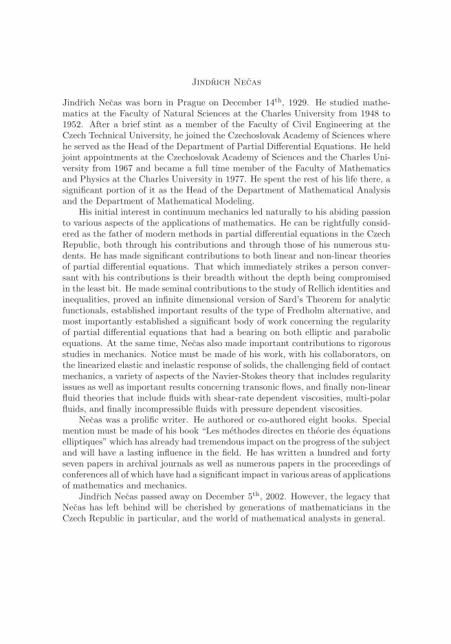
“topicsOnPartialDifferentialEquations” — 2008/1/7 — 16:30 — page 203 — #215
Jindrich Necas
Jindrich Necas was born in Prague on December 14th, 1929. He studied mathe-matics at the Faculty of Natural Sciences at the Charles University from 1948 to1952. After a brief stint as a member of the Faculty of Civil Engineering at theCzech Technical University, he joined the Czechoslovak Academy of Sciences wherehe served as the Head of the Department of Partial Differential Equations. He heldjoint appointments at the Czechoslovak Academy of Sciences and the Charles Uni-versity from 1967 and became a full time member of the Faculty of Mathematicsand Physics at the Charles University in 1977. He spent the rest of his life there, asignificant portion of it as the Head of the Department of Mathematical Analysisand the Department of Mathematical Modeling.
His initial interest in continuum mechanics led naturally to his abiding passionto various aspects of the applications of mathematics. He can be rightfully consid-ered as the father of modern methods in partial differential equations in the CzechRepublic, both through his contributions and through those of his numerous stu-dents. He has made significant contributions to both linear and non-linear theoriesof partial differential equations. That which immediately strikes a person conver-sant with his contributions is their breadth without the depth being compromisedin the least bit. He made seminal contributions to the study of Rellich identities andinequalities, proved an infinite dimensional version of Sard’s Theorem for analyticfunctionals, established important results of the type of Fredholm alternative, andmost importantly established a significant body of work concerning the regularityof partial differential equations that had a bearing on both elliptic and parabolicequations. At the same time, Necas also made important contributions to rigorousstudies in mechanics. Notice must be made of his work, with his collaborators, onthe linearized elastic and inelastic response of solids, the challenging field of contactmechanics, a variety of aspects of the Navier-Stokes theory that includes regularityissues as well as important results concerning transonic flows, and finally non-linearfluid theories that include fluids with shear-rate dependent viscosities, multi-polarfluids, and finally incompressible fluids with pressure dependent viscosities.
Necas was a prolific writer. He authored or co-authored eight books. Specialmention must be made of his book “Les methodes directes en theorie des equationselliptiques” which has already had tremendous impact on the progress of the subjectand will have a lasting influence in the field. He has written a hundred and fortyseven papers in archival journals as well as numerous papers in the proceedings ofconferences all of which have had a significant impact in various areas of applicationsof mathematics and mechanics.
Jindrich Necas passed away on December 5th, 2002. However, the legacy thatNecas has left behind will be cherished by generations of mathematicians in theCzech Republic in particular, and the world of mathematical analysts in general.

“topicsOnPartialDifferentialEquations” — 2008/1/7 — 16:30 — page 204 — #216
Jindrich Necas Center for Mathematical Modeling
The Necas Center for Mathematical Modeling is a collaborative effort between theFaculty of Mathematics and Physics of the Charles University, the Institute ofMathematics of the Academy of Sciences of the Czech Republic and the Faculty ofNuclear Sciences and Physical Engineering of the Czech Technical University.
The goal of the Center is to provide a place for interaction between mathemati-cians, physicists, and engineers with a view towards achieving a better understand-ing of, and to develop a better mathematical representation of the world that welive in. The Center provides a forum for experts from different parts of the worldto interact and exchange ideas with Czech scientists.
The main focus of the Center is in the following areas, though not restrictedonly to them: non-linear theoretical, numerical and computer analysis of problemsin the physics of continua; thermodynamics of compressible and incompressiblefluids and solids; the mathematics of interacting continua; analysis of the equationsgoverning biochemical reactions; modeling of the non-linear response of materials.
The Jindrich Necas Center conducts workshops, house post-doctoral scholarsfor periods up to one year and senior scientists for durations up to one term. TheCenter is expected to become world renowned in its intended field of interest.
ISBN 978-80-7378-005-0