topographic amplification of earthquakes in puerto rico

i

Topographic Amplification of Earthquakes in Puerto Rico and its Effects in Residential Construction

University of Puerto Rico at Mayagüez

Department of Civil Engineering, P.O. Box 9041, Mayagüez PR 00681 Tel (787) 265-3815, Fax (787) 833-8260

Email: [email protected] , [email protected]

Final Technical Report

VOLUME I

Numerical Study of the Amplification of the Seismic Ground Acceleration Due to Local Topography

FEMA-1247-DR-PR HMGP PR-0060B

Submitted to:

Lic. Melba Acosta

Governor’s Authorized Representative Commonwealth of Puerto Rico

Hazard Mitigation Office, P.O. BOX 9023434 San Juan, Puerto Rico 00902-3434

Mr. José A. Bravo

Disaster Recovery Manager Federal Emergency Management Agency

P.O. Box 70105 San Juan, Puerto Rico 00936-8105

By

Luis E. Suárez, Principal Investigator

Ricardo R. López, Co-Principal Investigator María Elena Arroyo Caraballo, Graduate Student

Drianfel Vásquez Torres, Graduate Student

Submitted: June 30,2003

i

Topographic Amplification of Earthquakes in Puerto Rico and its Effects in Residential Construction

EXECUTIVE SUMMARY

The objective of this project was to study the amplification of the earthquake

waves caused by topography, and to evaluate what effects should be expected on construction located in areas prone to suffer this phenomenon.

The research was divided in to two parts. The results presented in Volume I are concerned with the amplification of the seismic waves. Volume II deals with the effects on the structures, in particular residential constructions. It was found that most reinforced concrete houses built on slender columns are vulnerable to an earthquake amplified by the topography. A rehabilitation technique based on the addition of reinforced concrete walls is proposed in the recommendations in Volume II.

The research was carried out from November 2000 to May 2003. This investigation

was performed by:

Luis E. Suárez, Principal Investigator Ricardo R. López, Co-Principal Investigator Drianfel Vázquez Torres, Graduate Student María Elena Arroyo Caraballo, Graduate Student

The two volumes include the following information:

I. Volume I: Numerical Study of The Amplification of The Seismic Ground Acceleration Due to Local Topography. This investigation presents a study of the effects of local topography on the ground acceleration produced by earthquakes. The graduate student Maria Elena Arroyo Caraballo developed a Master of Science in Civil engineering thesis based on the subject of the first phase of the project.

II. Volume II: Seismic Behavior and Retrofitting of Hillside and Hilly Terrain

R/C Houses Raised on Gravity Columns. This investigation presents a study, by means of numerical simulation, of the seismic behavior of typical residences located at hills or hillsides and raised on gravity columns. The study takes into account the topographic amplification of the ground motion due to the location of the residences. The attention is focused on the seismic evaluation of the residences with typical geometric parameters obtained from a field survey carried out across Puerto Rico. Non-linear static pushovers and non-linear dynamic transient analyses are performed for the seismic vulnerability evaluation. The results of the analyses are used to select a seismic rehabilitation technique. As part of this investigation, the graduate student Drianfel Vázquez Torres submitted a dissertation in partial fulfillment of the requirements for the degree of Ph. D. in Civil engineering.

i

Abstract

This investigation presents a numerical study of the effects of local topography on the

ground acceleration induced by earthquakes. The attention is focused on the

amplification of the peak acceleration at the surface of the topographic irregularities.

Two-dimensional embankments and hills are studied. Four soil profiles defined in the

UBC-97 are used to define the material properties. The study is performed with the finite

element program QUAD4M. The seismic input is the acceleration time history of two

historic earthquakes with different characteristics. The nonlinear behavior of the soil is

taken into account with the Equivalent Linear Method. Two formulas that provide

amplification factors as a function of the geometry of the escarpment/hill at any point

along their surfaces are derived. The amplification factors found range from 1.00 to 2.35.

The case of an actual group of hills in Puerto Rico is examined, using real parameters and

a site-specific artificial earthquake.

ii

Compendio

En esta investigación se presenta un estudio numérico abarcador sobre los efectos

de la topografía en la aceleración del suelo causada por terremotos. La investigación se

concentra en estimar la amplificación de la aceleración pico en la superficie de

irregularidades topográficas. En particular, se estudiaron taludes y montañas, los cuales

se simularon mediante modelos de elementos finitos en dos dimensiones. Para definir las

propiedades de los materiales, se utilizaron cuatro perfiles de suelo definidos en el código

UBC-97. Para el análisis se utilizó el programa de elementos finitos QUAD4M. Los

datos de aceleración que se utilizaron fueron los historiales en el tiempo de dos

terremotos pasados. Se tuvo en cuenta el comportamiento no lineal del suelo mediante el

Método Lineal Equivalente. Como parte de la investigación se derivaron dos fórmulas

que proveen los factores de amplificación como función de la geometría de los taludes o

montañas en cualquier punto de su superficie. Se encontró que estos factores de

amplificación fluctúan entre 1.00 y 2.35. También se estudió un caso real de un grupo de

montañas en Puerto Rico, para el cual se utilizaron propiedades de los suelos específicos

del área, la geometría real de una sección transversal, y un terremoto artificial

especialmente generado para esta zona.

iii

Contents

List of Figures vi

List of Tables ix

I Introduction 1

1.1 Problem description . . . . . . 1

1.2 Previous works . . . . . . . 2

1.3 Scope of the thesis . . . . . . 7

1.4 General organization of the thesis . . . . 8

II Description of the General Methodology 11

2.1 Introduction . . . . . . . 11

2.2 Finite element concepts . . . . . 11

2.3 Description of the computer program QUAD4M . . 13

2.4 The pre and post processor Q4MESH . . . 17

2.5 The Equivalent Linear Model . . . . . 17

2.6 Finite element models . . . . . . 23

2.7 Seismic excitation . . . . . . 27

2.8 Boundary conditions . . . . . . 29

2.9 Guidelines for soil type categorization . . . 33

III Amplification of Seismic Motion Due to Escarpments 38

3.1 Introduction . . . . . . . 38

3.2 Slope stability analysis . . . . . . 48

3.3 General input data . . . . . . 43

iv

3.4 Selection of total height . . . . . 44

3.5 Escarpment amplification results . . . . 46

3.6 A general equation for the amplification factor . . 54

3.7 Nonlinear behavior of soils . . . . . 60

3.8 Summary . . . . . . . . 63

IV Amplification of Seismic Motion Due to Hills 65

4.1 Introduction . . . . . . . 65

4.2 General considerations . . . . . . 66

4.3 Ridge amplification results . . . . . 69

4.4 A general equation for the amplification factors . . 75

4.5 Frequency analysis . . . . . . 78

4.6 Summary . . . . . . . . 81

V A Case Study in Puerto Rico 82

5.1 Introduction . . . . . . . 82

5.2 Geographic conditions of Puerto Rico . . . 83

5.3 Site location . . . . . . . 85

5.4 Study of soils at the site . . . . . 88

5.5 Seismic excitation . . . . . . 91

5.6 The finite element model . . . . . 94

5.7 Results of the numerical simulation . . . . 95

5.8 Comparison with the proposed simplified methodology . 100

5.9 Summary and final comments. . . . . 100

v

VI Conclusions and Recommendations 102

6.1 Summary and conclusions . . . . . 102

6.2 Suggestions for further studies . . . . 105

References 108

vi

List of Figures

2.1 Linear and nonlinear shear-strain relationship . . . 18

2.2 Secant shear modulus . . . . . . 19

2.3 Shear modulus (a) and Damping ratio (b) curves . . 21

2.4 Stress Strain curve . . . . . . . 23

2.5 Dimensions of the escarpment model . . . . 24

2.6 Example of escarpment finite element mesh . . . 25

2.7 Dimensions of the ridge model . . . . . 26

2.8 Example of a finite element mesh of a ridge . . . 27

2.9 Acceleration time histories and Fourier Spectra for (a) El Centro

and (b) San Salvador earthquakes . . . . 29

2.10 Comparison of results using fixed and transmitting boundaries and extending the

mesh for the escarpment subjected to the El Centro

earthquake . . . . . . . . 31

2.11 Comparison of results (a) using transmitting boundaries (b) without

Transmitting boundaries at the sides and (c) extending the mesh,

for the ridge subjected to the San Salvador earthquake . 32

3.1 An example of an XSTABL result . . . . . 41

3.2 Escarpment heights . . . . . . . 45

3.3 Surface nodal points . . . . . . 47

3.4 Peak acceleration for a 15° slope escarpment . . . 48

vii

3.5 Amplification of the peak acceleration in a soil deposit without

irregularities . . . . . . . . 49

3.6 Comparison of the peak accelerations for a 30° escarpment

caused by both earthquakes . . . . . 50

3.7 Comparison of the peak accelerations for a 40° escarpment

caused by both earthquakes . . . . . 51

3.8 Peak acceleration for a 50° slope escarpment . . . 52

3.9 Peak acceleration for a 65° escarpment . . . . 53

3.10 Identification of parameters . . . . . 56

3.11 Amplification factor as a function of the escarpment’s height ratio

for a 40° slope . . . . . . . 57

3.12 The original line and the proposed equation for the 40° case . 60

3.13 Stress-Strain curve for a typical finite element . . . 62

4.1 Parameters for the equation of the parabola . . . 67

4.2 Nodes at the surface of the model of the hill . . . 70

4.3 Peak ground acceleration for a hill with n = 38 ft . . 70


4.5 Peak acceleration at the top of a soil deposit without irregularities 72



4.8 Parameters identification . . . . . . 75

viii

4.9 An example of a cubic trendline for n/m = 0.095 . . . 77

4.10 The cubic trendline and the general equation for n/m = 0.095 . 78

4.11 Comparison of ridge amplification subjected to El Centro

earthquake . . . . . . . . 79

5.1 Topographic view of Puerto Rico . . . . . 84

5.2 Residences located on the hill . . . . . 85

5.3 Map of the municipalities of Puerto Rico showing the location

of Guánica . . . . . . . . 85

5.4 View of the hill selected for study . . . . . 86

5.5 Topographic map of the case studied . . . . 87

5.6 View from road PR 116 of the Caño Hill . . . . 88

5.7 Soil map of the Valle de Lajas Area . . . . 90

5.8 Seismic activity in America and Caribbean . . . 98

5.9 Acceleration time history (a) and Fourier Spectrum (b) of the

artificial earthquake . . . . . . . 93-94

5.10 Finite element mesh for the Caño Hill . . . . 95

5.11 Coordinates for the Caño Hill mesh . . . . 96

5.12 Acceleration results for Caño Hill . . . . . 97

5.13 Average acceleration at different elevation . . . 98

5.14 Stress distribution . . . . . . . 99

5.15 Acceleration distribution . . . . . . 99

ix

List of Tables

2.1 Important Characteristics of the Earthquakes Selected . . 28

2.2 Soil Profile Types . . . . . . . 36

3.1 Total Height According to Material . . . . 46

3.2 Amplification Factors for an Escarpment:

El Centro earthquake (0.1g) . . . . . 54

3.3 Amplification Factors for an Escarpment:

San Salvador earthquake (0.1g) . . . . . 54

3.4 Amplification Factors for Different Escarpment’s Heights:

El Centro earthquake (0.1g) . . . . . 56

3.5 Most Critical Amplification Factors Considering Both Earthquakes 64

4.1 Maximum Amplification Factors for the Hill . . . 74

4.2 Amplification Factors for Hills of Different Heights . . 76

4.3 Most Severe Seismic Motions for the Analysis . . . 80

4.4 Summary of Maximum Amplification Factors for Different Hills 89

5.1 Materials Properties for the Model of the Caño Hill . . 93

5.2 Characteristics of an Artificial Earthquake for Puerto Rico . 98

5.3 Amplification and Deamplification Factors . . .

1

Introduction

1.1 Problem description

The study and analysis of damage during past earthquakes has shown that the

surface topography surrounding the site of the structures can considerably amplify the

ground motions. Although it is not currently considered, local site effects due to

topographic irregularities should play an important role in earthquake-resistant design.

There was evidence of this phenomenon in the 1976 Friuli and 1980 Irpino earthquakes

in Italy, and in the Chile earthquake of 1985.

Although this phenomenon has been known for several years and despite of its

importance for sites with pronounced surface irregularities, this effect is not considered in

the seismic codes. In particular, it has not been included in the US seismic codes and

thus in the design codes adopted for Puerto Rico. Probably one of the reasons why the

codes such as the Uniform Building Code disregard this phenomenon, is that in the US

mainland, with a few exceptions, the regions with conditions prone to topographic

amplifications are scarcely populated. Nevertheless, this phenomenon could be very

important in seismic prone zones that have this type of surface irregularities such as

Puerto Rico. The geography of the Island, along with the social and economic conditions

that affect the population distribution, makes many regions prone to topographic

amplification. The problem is aggravated by the many residential structures located on

hills and slopes that are constructed with weak first stories consisting of slender columns.

2

In addition, the amplification of the seismic motion can have potentially serious

consequences in terrains that are sensitive to landslides.

The topographic conditions can influence all of the important characteristics of a

strong ground motion, such as amplitude, frequency and duration. A few studies

concluded that, in addition to the magnitude amplification, the irregular topography could

cause a large increase in the duration of the motion. Although it has not received much

attention, this effect is worth of further studies. It is well known that motions of longer

duration increase the likelihood of resonance with the structures built on these regions. It

was also observed that the amplitude and phase of the ground motion vary rapidly along

mountain slopes, giving rise to differential motions. For those residential structures

supported by columns on steep slopes, the differential motion has potentially serious

consequences.

The main objective of the research described in this thesis is to develop a simple

methodology to take into account the amplification of the seismic waves that arrive to

hills or escarpments. In addition, the effect of the local topography of a region in Puerto

Rico on the potential earthquake motions will be used as a cased study.

1.2 Previous works

During the last decades several investigators have evaluated the effects of the

surface topography in the seismic response of the soil. The phenomenon has been

studied using different methodologies, analytical and numerical, as well as from

theoretical and experimental points of view. According to Geli et al (1988), it has been

3

reported that when destructive earthquakes are felt on hilly areas, those buildings at the

top of massive crests suffer more extensive damage than those located at the base.

Recent examples of this situation can be found in the 1976 Friuli and 1980 Irpino

earthquakes in Italy, and in the Chile earthquake of 1985.

Geli and his colleagues presented a brief review of experimental and theoretical

results on the effect of surface topography on seismic motions. They pointed out that the

two sets of results are only consistent on a qualitative basis. They speculate that the

differences are because the theoretical models are not sufficiently sophisticated. They

computed the response of a ridge with a smooth shape due to incoming SH waves, which

produce only out-of-plane displacements. They considered the presence of periodic

neighboring ridges and concluded that they may be responsible for the larger crest/base

amplifications observed. They also included subsurface layers in the model and

mentioned that it is difficult to separate their effects from those solely due to geometry.

They concluded that their results underestimate the actual amplification probably because

the more important SV and P waves were not considered.

Bouchon (1973) presented a study in which the topography was assumed to be

one-dimensional, and the displacements due to plane seismic waves incident on this

topography and coming from any direction were computed. For the analysis Bouchon

used a method developed by Aki and Larner (Bouchon, 1973) for the general case of

scattering of body waves in a layered medium having an irregular interface. A very

idealized seismogram was used to represent the earthquake. Bouchon concluded that the

effect of topography on surface motion appears to be very important when the

4

wavelength of the seismic wave is of the order of dimension of the anomaly, and it can

locally be responsible for both strong amplification and attenuation. The amplification is

very likely to occur at the top of the ridge whereas attenuation is probable at the bottom

of a depression. Bouchon was the first researcher to analyze the effects of incident in-

plane waves on ridges and valleys of an elastic homogeneous halfspace.

Castellani, Peano and Sardella (1982) proposed to use the finite element method

to study the effect of topography on the seismic ground motions because it provides more

realistic solutions and it can consider several factors that are not possible with analytical

techniques. For example, using finite elements one can achieve a detailed description of

the geometry of the topography and the subsurface layering. Moreover, it is possible to

include in the analysis the dissipation characteristics of the soils and their nonlinear

behavior when they are subjected to strong excitations. Castellani and his co-authors

explained how the finite element codes for plane strain can also be used for soil dynamic

problems dealing with the propagation of SH waves.

The effects of a ridge-like surface irregularity on the seismic response were

investigated by Athanasopoulos and Zervas (1993) using a 2-D finite element model.

The study considered the vertical propagation of SV waves due to four recorded

earthquakes. They found that the greatest values of amplification were obtained when the

base length of the ridge is two times the incident seismic wavelength for gentle slopes.

For steep slopes the worst case occurs when the two quantities are equal. The seismic

wavelength is defined as the product of the shear wave velocity vs of the soil on the ridge

and the dominant period Tpeak of the seismic waves. The value of Tpeak is defined as the

5

period with the highest ordinate in the response spectrum. The amplification factors

obtained by the authors range from 1 to 3.

As was mentioned previously, Italy is a country that is prone to suffer topographic

site effects. Sano and Pugliese (1999) reported that after the Ms 5.9 earthquake of

September, 26 1997 that hit the Umbria-Marche (a region in central Italy), the Italian

government decided that the amplification due to local effects had to be taken into

account in the post earthquake repair and reconstruction. The damaged area was located

on the Apennine Mountains, and thus the local soil amplification due to topographic

effects was important. Sano and Pugliese used a two dimensional code, based on the

indirect boundary element method, to investigate the phenomenon and also the effects of

geometric parameter changes. The numerical results show that the motion on a hill can

be highly variable from point to point and in a very short distance, depending on the

shape of the hill. Moreover, it was found that a small variation of the geometry, such as

changing the slope or the horizontal dimension of a hill, only affects the response at high

frequency and the space variability of the motion.

One of the leading authorities in topographic amplification is F. Sánchez-Sesma.

He contributed with a number of works to the study of the phenomenon (Sánchez-Sesma

1990, 1997, Sánchez-Sesma and Campillo 1993). Particularly useful is a chapter that he

prepared for a handbook of earthquake engineering (Sánchez-Sesma 1997). There the

author reviews the effects of local topography and local geology on strong seismic

motions. Sánchez-Sesma divided the various analytical methods proposed to predict site

effects in simplified configurations in three groups. They are: (1) the one-dimensional

6

propagation in a layered structure, (2) the two dimensional scalar wave propagation using

cylindrical eigenfunctions, and (3) some 2-D exact scalar and vector solutions based on

ray theory. Also the same author classified the numerical techniques developed for the

same purpose into two groups: domain and boundary methods. The finite element

method and the finite difference technique are examples of domain methods. These are

the most widely used methods by the geotechnical engineering community. An example

of the boundary methods is the boundary element method. This last technique is until

now mostly used by researchers. Nevertheless, the boundary methods have gained

increasing popularity. Other methods are the asymptotic techniques and the hybrid

methods that combine different techniques or the adaptation of approaches originally

devised to study other problems. To be able to solve the complex equations of motion,

the analytical methods are forced to use a simple geometry and to assume that the soil is

an elastic, homogeneous, isotropic and linear medium. As was mentioned before, due to

these assumptions the results obtained do not always agree with those measured at the

sites. However, these methods have the advantage that in some cases they can yield

closed-form solutions to the problem, which permit estimation of the effect on the

response of varying the different parameters. In other cases the analytical techniques

require the use of computers to evaluate the solution and the main benefit of using them

is lost. In addition, the analytical methods are very elaborate and require a mathematical

and geophysical background to understand them. Consequently, they are not useful for

the purpose of this thesis and they will not be further discussed here.

7

1.3 Scope of the investigation

The goal of the investigation is to assess the effects of topographic irregularities

on the earthquake-induced acceleration at the soil’s free surface such that this

phenomenon can be incorporated in seismic design codes. Two types of topographic

irregularities will be considered: an escarpment or slope and a hill or ridge. The idea is to

account for the effects of surface topography by means of a set of amplification factors.

These factors, when applied to the peak acceleration at the free field without irregularities

should give a conservative but reasonably accurate estimate of the peak acceleration

expected on the surface of the escarpments and hills. To achieve this goal, a parametric

study based on a numerical simulation of the phenomenon will be undertaken. The

numerical simulations will be carried out by means of finite element analyses of models

that include the topographic feature and the soil deposit underneath. Closed-form

equations defined only in terms of the parameters that describe the geometry of the

irregularity will be proposed to determine the amplification factors. In addition, the

amplification factors will be provided in tables. Since it is expected that the results will

be incorporated into guidelines or codes for the design of structures on zones with

topographic irregularities, the values of the amplification factors must cover the most

critical cases. This requires carrying out an extensive parametric study in which all the

major parameters affecting the phenomenon must be varied.

8

1.4 General organization of the investigation

Chapter I contains a general introduction to the investigation. The motivation and

problem description are briefly discussed. The chapter continues with a review of the

most relevant previous works on the subject of topographic amplification of earthquake

motions. The scope and organization of the investigation are also included in the first

chapter.

Chapter II contains a general description of the methodology used later in the

succeeding chapters to carry out the seismic analysis of the soil profiles below

topographic irregularities. There is a brief description of the computer program

QUAD4M for finite element (FE) analysis, which is the main tool used in this research.

There is also a discussion of the pre - and post - processor program Q4MESH, which is

used in conjunction with the previous program to generate the FE mesh and to visualize

the results. The procedure used by the program QUAD4M to account for the behavior of

soils with limited nonlinearities is discussed. The seismic excitations used as the input

for the analysis of the FE models are presented. The finite element model used to

describe the geometry of a soil deposit below a topographic irregularity on top is

introduced. The implications of the use of special boundaries in the FE program to

account for the unlimited extension of the soil in the horizontal directions are examined.

Finally, the chapter concludes with a description of the soil classification adopted for the

research.

In Chapter III begins the actual study of the amplification of the seismic motion

due to the presence of an irregular soil profile. Here the case of an escarpment or slope is

9

considered. The chapter starts with a description of a slope stability analysis carried out

using the program XSTABL. The objective of this analysis was to determine the highest

values of the angles of the slopes that can be naturally maintained with the soils

considered. In the next section, a selection of the total depth of the soil profile that

maximizes the amplification is presented. The core of the chapter that follows this

section, are the results of the amplification study for escarpments with increasing slope

angles. The results are presented in the form of graphs depicting the peak absolute

acceleration at the surface of the slope and at the horizontal level of the ground surface.

These results are next used to derive a general formula to calculate the amplification

factor as a function of the angle of the slope at any elevation. The mathematical

procedure followed to formulate the closed-form expression for the amplification factors

is explained. The chapter winds up with a discussion of the nonlinear behavior of the

analyzed soils when they are subjected to the earthquake ground motions selected for the

study.

Chapter IV is devoted to the study of the amplification of the earthquake shaking

on the surface of hills. The standard shape of the hill used in the FE models is described.

The main content of the chapter is the presentation of the results of the parametric study

done to quantify the amplification of the peak acceleration on the slopes of the hills. A

sample of graphs showing the peak acceleration in the nodes of the FE model at the top

surface is presented and discussed. Using the previous results, a general equation that

allows one to predict the amplification factors at a given height of a hill and as a function

of its aspect ratio is derived. The chapter ends with a discussion of some unexpected

10

results and a possible explanation based on a frequency analysis of the soil system and

the earthquake signals.

Chapter V contains a real case study of topographic amplification in Puerto Rico.

The site of a residential community located on the slopes of a group of hills was selected.

The community, known as Caño, is located in the municipality of Guánica in the south of

Puerto Rico. The elevation of the site was obtained from topographic maps. Using this

information, a two dimensional profile was prepared and modeled with plane strain finite

elements. The mesh was analyzed with the program QUAD4M. The properties of the

soil were defined by using soil maps, and by means of laboratory analyses of samples

taken at the site. The seismic input was obtained from a previous study carried out at the

Department of Civil and Surveying Engineering of the University of Puerto Rico at

Mayagüez. A synthetic earthquake, compatible with a design spectrum developed for the

city of Ponce, was applied at the location of the bedrock. A discussion of the findings

from the study and their implications are provided. The results obtained by applying to

this case the methodology developed in the previous chapter are presented along with a

comparison with the output of the specific numerical simulation.

The investigation ends up with the conclusions and recommendations presented in

Chapter VI. A summary of the main findings and achievements are discussed. A list of

areas and specific topics where it is deemed that more work would be beneficial is

provided.

11

CHAPTER II

Description of the General Methodology

2.1 Introduction

As it was discussed in the previous chapter, the topographic amplification of earthquake

waves has been studied for several years. The differences among these numerous studies

were the methodologies used. This thesis makes use of extensive numerical simulations

by means of a computer program based on the finite element method. The program

performs a finite element analysis of plane soil structures subjected to a horizontal

earthquake excitation at the base. The Equivalent Linear Method is used to

approximately take into account the nonlinear behavior of the soils subjected to strong

seismic motions. To create realistic analytical models it was necessary to simulate, as

accurate as possible, a soil deposit shaken by an earthquake. This includes using the

proper boundary conditions and soil profile, and the earthquake time history applied to

the base of the model. This chapter contains a discussion of all the concepts used in the

proposed methodology.

2.2 Finite element concepts

The finite element method (FEM) is a numerical procedure for analyzing structures and

continuous media. Usually the problem addressed is too complicated to be solved

satisfactorily by classical analytical methods. The problem may concern stress analysis,

heat conduction, or any of several other areas. The finite element procedure produces a

12

set of simultaneous algebraic equations in static cases or coupled ordinary differential

equations in dynamic problems, which are generated and solved on a digital computer.

The FEM models a structure as an assemblage of small parts or elements. Each element

is of simple geometry and therefore is much easier to analyze than the actual structure.

Elements are called “finite” to distinguish them from differential elements used in

analytical methods. The connection or dots between elements are called “nodes”. In

solid mechanics problems, the algebraic or differential equations that describe the finite

element model are solved to determine the displacements of the nodes representing

specific points of the structural system.

The power of the FEM resides principally in its versatility. The method can be

applied to various physical problems. The body analyzed can have arbitrary shape, loads,

and support conditions. The mesh can mix elements of different types, shapes, and

physical properties. User prepared input data controls the selection of problem type,

geometry, boundary conditions, element selection, and so on.

The FEM also has some disadvantages. A specific numerical result is found for

each specific problem: a finite element analysis provides no closed-form solution that

permits an analytical study of the effects of changing various parameters. A computer, a

reliable program, and intelligent use are essential to

obtain meaningful results. A general-purpose FE program has extensive documentation

with which one must be familiar before attempting to use it. Experience and good

engineering judgement are also needed in order to define a good model. Many input data

13

are required and voluminous output must be sorted out and understood (Cook et al,

1989).

2.3 Description of the computer program QUAD4M

The finite element method has shown to be a powerful tool for the solution of

various problems in continuum mechanics. Although its use is not widespread in their

communities, the FEM is a very useful technique for the geotechnical engineers.

However, it has been applied extensively for the evaluation of the seismic response of a

variety of soil deposits and earth structures (Idriss et al. 1973). The displacement-based

formulation of the FEM is typically used for geotechnical applications and the results are

presented in the form of displacements, stresses and strains at the nodal points. To select

a suitable program, the user must consider the implementation of the constitutive model

and the availability of different types of finite elements such as triangular or quadrilateral.

A number of programs to solve geotechnical problems using time domain solutions as

well as frequency domain solutions have been written in the past 30 years.

In 1973 researchers at the Department of Civil Engineering of University of

California at Berkeley developed the program QUAD4 for the seismic response of soil

structures (Idriss et al. 1973). This program is essentially a two dimensional variable

damping finite element procedure. The analytical procedure implemented in the program

permits the use of both strain-dependent modulus and damping ratios for each element in

the finite element representation of a deposit. This was an improved tool to perform a

response analysis of soil deposits having considerable geometric variations and having

14

greatly varying material characteristics. In addition, the formulation allows for the

incorporation of nonlinear stress-strain relationships through the use of equivalent linear

and strain dependent material properties. The equations of motion are solved by a direct

step-by-step numerical method. The output from the program includes the maximum

values of the horizontal and vertical accelerations along with their time of occurrence,

and a time history for the shear strain in each element. In 1994 researchers from the

University of California at Davis modified the original program QUAD4 to include a

compliant base. This version is known as QUAD4M (Hudson et al. 1994).

Likewise the original code, QUAD4M is a dynamic, time domain, equivalent linear two-

dimensional computer program. The implementation of a transmitting base, an improved

time stepping algorithm, seismic coefficient calculations, and a restart capability are the

improvements undertaken in the new program.

The evaluation of the seismic response is carried out by solving in the time domain a

system of equations represented in matrix form as:

[ ] [ ] [ ]{ } { } g

.....uRuKuCuM =+

⎭⎬⎫

⎩⎨⎧+

⎭⎬⎫

⎩⎨⎧

(2.1)

where dots represent differentiation with respect to time and:

{ } vector nt displaceme relative u

u direction one in on accelerati outcropg

..

[ ] matrix mass M

15

[ ] matrix dampingC

[ ] matrix stiffnessK

[ ] R rvector load }]{Μ[− =

{ } tscoefficien influence withvector r

The time stepping method previously used in QUAD4 (the Wilson-θ method) was

changed in QUAD4M. To obtain the displacement, velocity and acceleration at each

time step the program now uses the Trapezoidal rule.

It was mentioned that the new program QUAD4M has absorbing boundaries

implemented to allow for the reduction in the size of the FE mesh. The concept of

absorbing or viscous boundaries for FE models of infinite or semi-infinite domain was

first introduced in 1969 by Lysmer and Kuhlemeyer (Hudson et al. 1994). They

suggested the use of dampers or dashpots with proper constants to absorb the P, S, or

Rayleigh waves impinging on the borders of the model. The viscous dampers are applied

in two orthogonal directions at each of the nodes that make up the base as well as in those

nodes at the sides of the semi-infinite model. To implement these dampers in the

computer code, the damping coefficients of the dashpots are added to the appropriate

diagonal terms of the total damping matrix.

It was mentioned that QUAD4M could also compute the seismic coefficient. This

coefficient is defined as the ratio of the force induced by the earthquake in the block of

16

the mesh with respect to the weight of that block. This parameter is computed for each

time step.

To model the damping in soils, QUAD4M uses the Rayleigh damping

assumption. However, opposed to most well known FE programs, the Rayleigh damping

matrix is defined for each finite element. For each element q the damping matrix is

formulated as follows:

[ ] [ ] [ ]qqqqq KMC β+α= (2.2)

The damping matrix of the full model is constructed by assembling the element

matrices in the usual way. The coefficients α and β are selected by specifying damping

ratios at two frequencies. One frequency is chosen as the fundamental frequency ω1 of

the model. The second frequency is established as a multiplier of the fundamental

frequency. The value ω1 of the system is internally calculated using the formula obtained

from a continuous and homogeneous soil deposit that can only withstand shear

deformation. The output file displays the two frequencies at which the damping ratios

were set.

Additional modifications made to the original QUAD4 program were aimed at

making the new program conform to a structured FORTRAN language and implementing

data structures to describe the elements and nodes (Hudson et al. 1994).

17

2.4 The pre and post processor Q4MESH

The US Army Engineer Waterways Experiment Station (now the Engineering

Research and Development Center) under the sponsorship of some organizations,

developed a pre- and post processor called WINMESH for use with the finite element

program STUBBS. WINMESH is a finite element pre-processor, a post-processor, and a

menu-driven input file builder created as a productivity tool to be used with the

geotechnical finite element program STUBBS (Peters and Kala 1999).

A new pre and post processor, Q4MESH was generated by the Engineering

Research and Development Center. This work was carried out as part of the investigation

reported in this thesis. It is a combination of the WINMESH and QUAD4M programs

into a new one, which has more capabilities and is more user-friendly. The pre processor

has the capability to graphically build a mesh file, assign material properties and

boundary conditions which can be pasted into a text file to be used as input file for

QUAD4M. The post processor can display plots of stresses or strains on the mesh, and

acceleration time histories. The pre and post processor was based on the WINMESH

program. The Q4MESH program is CAD-like and permits the user to select elements

and nodes using the “mouse”. The technique used is called “rubberbanding”. Initially,

only the menu referred to, as FILE is active. The brief description of the input of

Q4MESH is just to provide an overview, because the program is more powerful.

2.5 The Equivalent Linear Model

18

When a strong earthquake affects a soil deposit, it can produce strains in the

material of such magnitude that the soil behaves in a nonlinear fashion. Therefore, to

perform a site response analysis for this case, one must know the stress-strain relationship

of a soil subjected to a shear state. For the case of small strains such as those induced by

a weak to moderate earthquake, the soil follows the Hooke’s law for shear, i.e.:

γ=τ oG (2.3)

For more severe cases of seismic excitation, the Hooke’s law must be replace by a

nonlinear constitutive equation with a form

( )γ=τ f (2.4)

such as the one illustrated in Figure 2.1

Figure 2.1 Linear and nonlinear shear-strain relationship

In 1970, H. B. Seed and I. M. Idriss developed a procedure to consider

approximately the nonlinear behavior of soils in dynamic problems that became known as

the Equivalent Linear Method. The main idea of this method is to obtain similar results

to those obtained from a truly nonlinear analysis by means of a series of linear analyses

γ

τ

τ=f(γ)

τ≈Goγo

19

utilizing ”effective” values of the shear modulus and damping. The effective shear

modulus or secant shear modulus is approximated as (Kramer 1996),

c

csecG

γτ

= (2.5)

where:

amplitude strain shear cγ

amplitude stress shearcτ

Thus, as shown in Figure 2.2, Gsec describes the general inclination of the hysteresis loop.

The effective damping ratio ξeff is the area Ahyst inside the hysteresis loop corresponding

to γc, divided by the elastic energy corresponding to the same deformation level, as

illustrated in Figure 2.2, i.e.:

2

csec

hyst2

csec

hysteff

G2

A

2G

A41

γπ=

γπ=ξ (2.6)

Figure 2.2 Secant shear modulus

20

Of course, the values of γc are not known in advance, since they are calculated from the

solution of the equations of motion. Therefore, it is necessary to implement an iterative

process to calculate the effective shear modulus and effective damping ratio. The process

starts by estimating initial values for the shear modulus and damping ratio. The response

of an equivalent linear system defined using these values can be calculated in the time

domain with modal analysis or numerical integration, or in the frequency domain using

the discrete Fourier transform. Using the assumed initial values of the modulus and

damping, the maximum shear strains for each element in the model are calculated. With

these new values, the previously assumed values of Geff and ξeff are corroborated. The

procedure requires knowing how Geff and ξeff vary with the shear strain. If one adopts a

specific nonlinear constitutive equation, say for instance the hyperbolic model, then it is

possible to obtain analytical expressions relating the effective parameters to γ.

Alternatively, one can provide tables that relate Geff and ξeff to γ at certain values. This is

the approach adopted in QUAD4M. The program uses curves proposed by Seed and

Idriss of Geff and ξeff for different type of soils shown in Figure 2.3.

21

(a)

(b)

Figure 2.3 Shear modulus (a) and Damping ratio (b) curves

Entering these curves with the shear strains in the x-axis, the equivalent Geff and ξeff can

be verified and updated, if needed. In the latter case, these new values are used to

generate new stiffness and damping matrices. The response is again obtained with a

linear analysis, and the shear strains are used to find Geff and ξeff. The process finishes

0100020003000400050006000700080009000

10000

0.0001 0.001 0.01 0.1 1

Shear Strain

Shea

r Mod

ulus

(ksf

)

Clay material Gravel material

0

5

10

15

20

25

30

0.0001 0.001 0.01 0.1 1

Shear Strain

Dam

ping

Rat

io (%

)

Clay material Gravel material

22

when the differences between the most recent values and those from the previous cycle

are acceptable. The most recently updated values of the shear strain, stress or

displacement obtained at the last iterative step are considered to represent a good

approximation of the actual nonlinear solution.

The Equivalent Linear Method was compared on several occasions with real

nonlinear analyses and it was found that the results predicted by the former are

satisfactory provided there is convergence. The Equivalent Linear method, however, is

not exempt of problems. For example, one of the drawbacks associated with the method

is that there is no proof of convergence. Moreover, some difficulties were reported when

it was applied to problems involving deconvolution of the seismic waves, i.e. finding the

signal at the bottom of the deposit when it is known at the surface.

Nevertheless, and despite these problems, the Equivalent Linear method is widely

used in geotechnical earthquake engineering. It is important to bear in mind that a truly

nonlinear analysis requires much more time from the analyst and the computer, and it

also requires knowing more parameters for each soil layer to define the constitutive

model. The diversity of soil properties and the uncertainty in some of them contribute to

increase the popularity of the Equivalent Linear method. Another reason that plays an

important role in the acceptance of the method is its widespread implementation in

computer programs for geotechnical earthquake engineering. For example, in addition to

the computer program used in this research, the popular program SHAKE that evaluates

the seismic response of one-dimensional soil deposits employs the method. Figure 2.4

23

presents an example of the shape of the stress-strain relationship of a soil used in the

QUAD4M program.

Figure 2.4 Stress Strain curve

2.6 Finite element models

Two types of surface topography were considered in this research to quantify the

amplification in the ground acceleration due to the seismic waves. The soil deposit was

first modeled with an escarpment and later with a ridge or hill. To study the escarpment

it was necessary to establish somehow a reduced number of dimensions for the model

among the infinite possible configurations. The mesh of the FE model was created using

the interface program Q4MESH and the analysis was carried out using the finite element

program QUAD4M. Different types of escarpments were analyzed. The depth H of the

block of soil under the escarpment was selected as two times the height of the

escarpment. The total height h+H depends on the type of soil and is selected so that the

amplification is maximized, as explained in Chapter III, Section 3.4. The lateral

0

20

40

60

80

100

120

0 0.005 0.01 0.015 0.02 0.025 0.03

Shear Strain, γ

She

ar S

tress

(ksf

)

24

extension of the finite element mesh far beyond the toe and top of the slope was taken

into account by using viscous boundaries. The horizontal distances to the boundaries a

were selected as two times the horizontal distance of the ridge L, as illustrated in Figure

2.5.

Figure 2.5 Dimensions of the escarpment model

To obtain amplification factors for the many configurations that can be found in real

situations, it was necessary to examine different cases. The angle of the slope was

chosen as the variable parameter that distinguish the different models. Five element

meshes were used to model different inclination angles of the escarpment. This

inclination angle was selected by a slope analysis to avoid static stability failure and

using a correlation between the critical height and the material properties. The angles

considered were 15, 30, 40, 50 and 65 degrees. Four types of soil profiles were also

considered, although some materials do not resist angles of slopes greater than the

friction angle of the soil. These types of soils and the details of the slope stability

α

h

H=2h

a =2L L a =2L

25

analysis are presented in the next chapter. Figure 2.6 presents an example of a typical

escarpment finite element model used in this research.

Figure 2.6 Example of escarpment finite element mesh

For each case the output of the program QUAD4M included peak nodal

accelerations and peak element stresses. As mentioned previously, to carry out the

dynamic analysis QUAD4M performs a number of iterations that is fixed by the user in

the input data. To guarantee that the process converges to a reasonable extent, in all the

cases studied the maximum number of iterations was set equal to ten. At this number of

iterations, the final differences in percent in the shear modulus and damping ratio at two

consecutive steps were approximately zero. A higher number of iterations was not

considered necessary nor justified, especially taken into account that hundreds of

computer runs would be carried out throughout the study.

The other cases analyzed were the topographic irregularities with the shape of

ridges. Evidently, in this case also one can have an infinite number of shapes to describe

the ridge’s geometry. Many of the ridges previously studied in the literature had the

26

shape of a wedge. This was done mostly to facilitate the analysis, but we did not

consider this as a realistic shape. Therefore, it was decided to use a “smooth” shape to

describe the ridge. Since a parabola has the advantage that by varying the three

coefficients in its equations its shape can be easily manipulated, it was chosen as the

geometry of the ridge. The ridges were defined by two parameters: its base length m, and

the total height of the ridge, n. Viscous boundaries are used to take into account the

theoretically infinite lateral extension of the finite element mesh along the left and right

sides. The lateral extension of the FE mesh beyond the ridge’s toe is defined by a and it

was set equal to m/2, as illustrated in Figure 2.7. The depth of the soil deposit under the

hill is H and it was taken equal to a/2.

Figure 2.7 Dimensions of the ridge model

The parameter n was varied during the numerical simulation study and four

models were analyzed. As it was done in the case of the escarpment, a slope stability

analysis was carried out to evaluate the critical height. The stability analysis is discussed

in Chapter IV. The value of m was kept constant and by varying n different aspect ratios

of the ridge was examined. The values of n used for the study were 38, 75, 115 and 225

ft. There is no particular reason for selecting those values. The first value of n used in

2m

ma = m/2 a = m/2

n

H = a/2

27

the preliminary studies was 75 ft and the other values were chosen a posteriori to cover a

reasonable range. The value of m was fixed at 400 ft and thus the aspect ratios of the hill

are approximately equal to 0.1, 0.2, 0.3 and 0.6. The English or fps system of units was

used throughout the analysis. Figure 2.8 illustrates an example of a typical finite element

mesh of a ridge used in the study. Finally, all the finite element models of the ridge and

deposit were analyzed using ten iterations in the Equivalent Linear method to obtain

results with a reasonably accuracy.

Figure 2.8 Example of a finite element mesh of a ridge

2.7 Seismic excitation

The seismic excitation, defined as an acceleration time history, was applied to the

base of the model, that is, to the bedrock. The recorded horizontal accelerogram of two

historical earthquakes, namely the El Centro and San Salvador earthquakes, were used as

input motion for all the finite element models. The El Centro earthquake occurred on

May 18, 1940 and the San Salvador was more recent: it occurred on October 10, 1986

28

causing approximately 1000 deaths. Table 2.1 shows the most important characteristics

of both seismic events (Strong Motion Data Center 1999).

Table 2.1 Important Characteristics of the Earthquakes Selected

Earthquake Magnitude

(Richter Scale)

Peak

Displacement

(cm)

Peak Velocity

(cm/s)

Peak

Acceleration

(cm/s2)

El Centro 7.1 10.87 33.45 341.70

San Salvador 5.5 11.90 80.00 -680.80

The original peak ground acceleration of both seismic records was scaled to 0.1g. This

was done so that the soils would behave linearly or with limited nonlinear excursions.

For a given seismic input, the nonlinear behavior of the soils tends to reduce the absolute

accelerations at the free surface, compared to a soil with a linear response. Therefore,

since we are interested in determining maximum amplification factors and not the actual

accelerations due to the earthquakes selected, it was considered prudent to limit the level

of the seismic excitation.

This hypothesis was proved by running trial cases. The two earthquake records

were selected in order to use seismic input time histories with different characteristics.

Figure 2.9 displays the acceleration time histories and the Fourier spectrum for the two

earthquakes used in the study. The El Centro accelerogram is typical of a broad band

process while the San Salvador represents a narrow band process.

29

(a)

(b)

Figure 2.9 Acceleration time histories and Fourier Spectra for (a) El Centro and (b) San Salvador earthquakes

2.8 Boundary conditions

To increase the computational efficiency, it is desirable to minimize the number

of elements in a finite element model. For many soil response analysis and soil structure

interaction problems, rigid or near rigid boundaries (such as those representing the

0 5 10 15 20 25 30 35 40 45 50

-0.06

-0.04

-0.02

0

0.02

0.04

0.06

0.08

0.1

Time [sec]

Acc

eler

atio

n [%

g]

0 10 20 30 40 50 60 700

200

400

600

800

1000

1200

1400

1600

Frequency [rad/sec]

Am

plitu

de

0 1 2 3 4 5 6 7 8 9-0.1

-0.08

-0.06

-0.04

-0.02

0

0.02

0.04

0.06

Time [sec]

Acc

eler

atio

n [%

g]

0 10 20 30 40 50 60 700

100

200

300

400

500

600

700

800

Frequency [rad/sec]

Am

plitu

de

0 1 2 3 4 5 6 7 8 9-0.1

-0.08

-0.06

-0.04

-0.02

0

0.02

0.04

0.06

Time [sec]

Acc

eler

atio

n [%

g]

0 10 20 30 40 50 60 700

100

200

300

400

500

600

700

800

Frequency [rad/sec]

Am

plitu

de

30

bedrock) are located at considerable distances, particularly in the horizontal direction,

from the region of interest (Kramer 1996). By doing this, the errors introduced by the

spurious reflections of the seismic waves at the rigid boundaries are minimized.

However, the price to pay is an increase in the number of elements, degrees of freedom

and execution time of the program.

The new version of QUAD4M has the option of using a so-called compliant base in the

soil mass. This is a better way of dealing with infinite field conditions, because it

permits minimizing the number of elements that represent the underlying half space.

When a transmitting base is used, the input motion is a function of the materials

properties of the half space below the mesh and the properties and geometry of the mesh.

In all cases analyzed the soil deposit is assumed to be underlain by a half space having a

shear wave velocity of 3000 ft/sec, a compression wave velocity of 7000 ft/sec and a unit

weight of 135 pcf. To assess whether the dimensions of the meshes to be used later are

acceptable, different boundary conditions were first considered. This was done for both

topographic features, the escarpment and the hill. The analysis consisted in comparing

the responses obtained with an original FE mesh, the same mesh but with transmitting

boundaries, and with another extended mesh without the special boundaries. All the

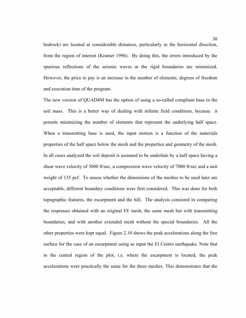
other properties were kept equal. Figure 2.10 shows the peak accelerations along the free

surface for the case of an escarpment using as input the El Centro earthquake. Note that

in the central region of the plot, i.e. where the escarpment is located, the peak

accelerations were practically the same for the three meshes. This demonstrates that the

31

transmitting boundaries are capable of absorbing the energy of the seismic waves that

arrive at the sides.

Figure 2.10 Comparison of results using fixed and transmitting boundaries and extending the mesh for the escarpment subjected to the El Centro earthquake

The analysis was repeated with a ridge. In this case the accelerogram used was

that of the San Salvador earthquake. From the time history results produced by the

program, the peak accelerations at the free surface were retrieved and are plotted in

Figure 2.11 as a function of the horizontal position. As it is illustrated in Figure 2.11,

after the mesh reaches a sufficient length, extending further the mesh does not change the

peak acceleration in the region of the hill. Therefore, for all the future analysis the FE

mesh to be used will be the original (i.e. that with the shorter length) mesh with

transmitting boundaries.

0

0.05

0.1

0.15

0.2

0 100 200 300 400 500 600 700

Horizontal Distance (ft)

Peak

Acc

eler

atio

n (g

)

w ith transmitting boundaries on the sides

w ithout transmitting boundaries on the sides

respective nodes on the long mesh

32

(a) (b)

(c)

Figure 2.11 Comparison of results (a) using transmitting boundaries (b) without transmitting boundaries at the sides and (c) extending the mesh, for the ridge subjected to

the San Salvador earthquake

0

0.05

0.1

0.15

0.2

0.25

0 100 200 300 400 500 600 700 800 900


Pea

k A

mpl

ifica

tion

(g)

n=75, total length=800

0

0.05

0.1

0.15

0.2

0.25

0 100 200 300 400 500 600 700 800 900

Horizonta l Distance (ft)

Pea

k Am

plifi

catio

n (g

)

n=75 , total length=800

0

0.05

0.1

0.15

0.2

0.25

0 500 1000 1500 2000 2500


Pea

k A

mpl

ifica

tion

(g)

n=75, total length=2400

33

2.9 Guidelines for soil type categorization

Some researchers pointed out that it is very difficult, if not impossible, to separate

the amplification due to the topographic irregularity from that due to the local geological

conditions. In other words, the effects of the type of soil and the discontinuity in the

geometry are interwoven and they must be considered simultaneously. Therefore, to

carry out the research presented in this thesis, it was necessary to select the types of soil

that will be assumed for the escarpments and hills as well as for the soil deposit

underneath them. Depending on the specific purpose, there are a number of soil

classifications available. Since the objective of the present study is to develop a simple

methodology such that the effect of the local topography can be incorporated into seismic

codes, it was decided to use the classification presented in these documents. Puerto Rico

recently adopted the 1997 edition of the Uniform Building Code (UBC-97) as its official

design and construction code (ICBO 1997). Therefore, it was decided to use the soil

profile types listed in this code to categorize the material of the deposits, slopes and

ridges.

The soil profile types in the UBC-97 are defined in terms of three alternative

parameters. The main one is the average shear wave velocity, that is the average value of

the velocity of propagation of S waves along the different layers of a soil deposit. The

shear wave velocity is characteristic of a given material and, for a given soil, it is a

function of its shear modulus G and mass density ρ.

According to the UBC-97, the average shear wave velocity sV−

is determined as

34

∑

∑

=

=−

=n

1i si

i

n

1ii

s

vd

dv (2.7)

where:

deposit the in layers different of numbern

(m) feet in layer of thickness di i

(m/sec)ft/sec in layer ofvelocity waveshear vsi i

i

isi

GV ρ=

Another alternative parameter used to classify the soils in the UBC-97 is the

average standard penetration resistance−

N. This parameter gives information concerning

the degree of compactness or stiffness of the soil in situ. It is defined as

∑

∑

=

=−

=n

1i i

i

n

1ii

N

d

dN (2.8)

∑=

−=

n

1i i

i

sCH

N

N dd

(2.9)

where:

(mm) feet in layer of thickness di i

35

m) (30.48 feet 100 top the in layers soil sscohesionle of thickness total the ds

standards recognized nationally approved withaccordance

in layer soil of resistance n penetratio standard the Ni i

The term NCH is the standard penetration resistance for cohesionless soil layers.

Cohesionless soils are granular materials such as sand or gravel. In these types of soils,

the resistance depends on the effective overburden pressure. In homogeneous conditions,

it means that the resistance augments as the depth increases. The behavior of this type of

soil requires special attention, and for this reason it is important to evaluate if there exist

layers of cohesionless materials in the soil deposit.

The third and last property used by the UBC-97 to categorize the type of soil is

the average undrained shear strength. This is an important parameter related to porewater

pressures. It is especially important in soft clays and silts under static conditions and in

loose sands under dynamic loading. According to the UBC-97, this parameter is

calculated using the following formula,

∑=

−

=n

1i ui

i

cu

Sd

dS (2.10)

where:

m) (30.48 feet 100 top the in layers soil cohesive of ds) - (100 thickness total the dc

36

(250kPa) psf 5,000 exceed to not standards, recognized nationally approved withaccordance in strength shear undrained the Sui

The formulas given before as well as the range of values provided in Table 2.2 (taken

from the UBC-97) are used to determine the type of soil profile.

Table 2.2 Soil Profile Types (International Conference of Buildings Officials 1997)

1 Soil Profile Type SE also includes any soil profile with more than 10 feet of soft clay defined as a soil with a PI>20, wmc�40% and Su<500 psf .

The material properties required to define the soil in the FE program are the unit

weight, the Poisson ratio and the shear modulus. For a given soil type, it is assumed that

these three parameters have the same values for all cases. As it was pointed out, the

analytical models were evaluated using the soil types in the UBC-97, and the average

shear wave velocity was used to classify them. The soil profile types SA and SF were not

considered in this study. The soil SA is classified as a hard rock (VS > 5000 ft/s) and it is

estimated that this soil is not common in Puerto Rico since it is characteristic of regions

in the eastern US.

The soil classified as SF was not used in the research because it requires a site-

specific evaluation and thus the general results and formulas obtained in this study would

Soil Profile Soil Profile Name/ Shear Wave Velocity, Standard Penetration Test, N [or NCH Undrained Shear Strength,Type Generic Description Vs feet/sec (m/s) for cohesionless soil layers] (blows/foot) Su psf (kPa)

SA Hard Rock >5,000 (1,500) _ _SB Rock 2,500 to 5,000 (760 to 1,500)SC Very Dense Soil and Soft Rock 1,200 to 2,500 (360 to 760) >50 >2,000 (100)SD Stiff Soil Profile 600 to 1,200 (180 to 360) 15 to 50 1,000 to 2,000 (50 to 100)SE

1 Soft Soil Profile <600 (180) <15 ,1,000 (50)SF

Average Soil Properties For Top 100 Feet (30 480 mm) of Soil Profile

Soil Requiring Site-specific Evaluation

37

not be applicable anyway. The values of the shear wave velocity for the different soil

profiles used throughout the present study are the following:

SB: 3750 ft/s

SC: 1850 ft/s

SD: 900 ft/s

SE: 575 ft/s

38

CHAPTER III

Amplification of Seismic Motion Due to Escarpments

3.1 Introduction

This chapter presents a description of the finite element analyses of escarpments

subjected to acceleration time histories at the bedrock. The results obtained from the

studies of many different escarpment configurations of different heights and made up of

several soil types are presented. Using these results, amplification factors that relate the

peak ground acceleration to the peak acceleration at the escarpment’s free surface are

derived. Although the goal of the present study is to examine the effect of surface

irregular topography in the seismic motion, it is important to consider that when soil

deposits are subjected to cyclic loads, they can present some type of failure. The

combined effect of seismic loads and the changes in shear strength will result in an

overall decrease in the stability of slopes. Therefore, before undertaking the seismic

amplification of the escarpments, a slope stability analysis is carried out.

3.2 Slope stability analysis

Approximately 40 percent of the US population are exposed to effects of

landslides. Landslides often are triggered by natural events such as floods, earthquakes

and volcanic eruptions. The slope failures are usually due either to a sudden or gradual

loss of strength by the soil or to a change in geometric conditions. The main items

required to evaluate the stability of a slope are: (1) the shear strength of the soils, (2) the

39

slope geometry, (3) the pore pressures or seepage forces and, (4) the loading and

environmental conditions (Abramson et al 1996).

The first task undertaken before performing the analyses presented in this chapter

was to establish what inclination angles could be realistically used for further time history

studies. A computer program was used for this purpose: the program XSTABL

(Interactive Software Designs 1995). This program consists of two interactive, but

separate portions: (1) the data preparation interfaces and, (2) the slope stability analysis

programs. The program performs a two-dimensional limit equilibrium analysis to

compute the factor of safety for a layered slope.

For the analysis of the stability of a slope it is important to know the geometry

and the subsoil conditions. The result of the analysis, i.e., the factor of safety, is a vital

parameter in the design of slopes. The lower the quality of the site investigation, the

higher the desired factor of safety should be, particularly if the designer has only limited

experience with the materials in question.

A number of slopes were selected to verify their stability. The angles of the

slopes varied from 15 degrees to 75 degrees, in increments of ten. The program

XSTABL permits to construct the slope profile using coordinates, to establish the soil

parameters, to define the water table condition, to select the analysis that the user prefers,

and to apply loads. In all the cases the program performs a pseudo-static analysis to

simulate the effects of an earthquake. An average horizontal seismic coefficient of 0.15

was entered in the data table. This is a typical value for the seismic coefficient, the Corps

of Engineers use in the practice and also the same value generated by Seed (1979). The

40

method of analysis used was the Simplified Bishop Method. This method was used to

identify the critical surface with the lowest factor of safety. This method satisfies vertical

force equilibrium for each slice and overall moment equilibrium about the center of a

circular trial surface. To simulate more realistic conditions, a phreatic surface was

included in the models analyzed. In the program the free groundwater level defines the

phreatic surface, or the phreatic line in two dimensions. Proceeding in this way, the value

of the factor of safety calculated will be conservative.

As mentioned previously, if the designer does not know the characteristics of the

site, for example the soil properties, it is very difficult to determine a factor of safety and

the critical surface. Many cases were studied by changing soil parameters such as the

cohesion and friction angle. Cohesionless and cohesive soils were analyzed using a unit

average weight of 125 pcf. When site investigations are carried out, they usually show

that to find a unique type of material in a region is nearly impossible. A typical cohesive

soil (clay) was studied and the results show that the critical surface is located outside the

slope. In this case, when the critical surfaces are not generated in the face of the slope, it

is due to the component of cohesion in the soil particles. The majority of the cases

examined presented a failure surface that went from the toe of the slope to the top. The

ground water table lies at the toe of the slope and is illustrated in Figure 3.1 as w1. This

behavior is the opposite of the one found for cohesive materials. It means that the

inclination angles are unstable using these kind of material properties.

41

The profile, the free groundwater level, the lower limit and the most critical

surfaces are illustrated in Figure 3.1. This figure shows an example of many cases

considered.

Figure 3.1 An example of an XSTABL result

The output of the program provides ten critical surfaces, the coordinates of the

center of the circle that produces the critical surface, and the factor of safety for this

method. After many cases were considered and the results analyzed, it was decided that

the slopes from 15 to 65 degrees would be studied with the QUAD4M program. The

slope of 75° was eliminated due to the small value of the factor of safety obtained. For

this study, the values of the factor of safety that were considered acceptable were those

greater than 1.1. It is important to have in mind that for seismic design the values should

be higher. However, since the analysis carried out did not consider a mixture of different

materials, values greater than 1.1 were regarded as acceptable.

It is important to mention that not all the amplification factors for slopes are

presented, because other soil parameters are also considered in the stability analysis. For

example, the materials have different properties as cohesion and angle of internal friction.

For slope stability analysis, it is very important to know the maximum slope that the soil

resists. This is measured by the angle of repose, which is the angle between the

42

horizontal and the maximum slope that a soil can assume through natural processes. For

dry granular soils, the effect of the height of slope is negligible; for cohesive soils, the

effect of height of slope is so important that the angle of repose is meaningless.

Therefore, the angle of repose is a critical parameter for non-cohesive materials. Those

angles can reach up to 40° depending on the loose or dense soil condition. The angle of

repose depends on:

1. The size and particle shape - large, angular particles have steeper angle of repose

2. Sorting - well-sorted materials have a higher angle of repose

3. Composition of particles - stronger particles will have a steeper angle of repose

Cohesive materials like clays, silts and rocks are able to maintain very high slope angles

(up to 90° as a cliff).

Other factor that is used to evaluate the stability of slopes is the height. A slope

underlain by clean dry sand is stable regardless of its height, provided that the angle

between the slope and the horizontal is equal to or smaller than the angle of internal

friction. A cohesive material can stand a vertical slope at least for a short time, provided

the height of the slope is less than HC, which is defined as

γ

= uC

S4H (3.1)

where:

strength shear undrainedSu

weightunit soil γ

43

If the height of a slope is greater than HC, the slope is not stable unless the slope

angles β are less than 90°. The greater the height of the slope, the smaller must be the

angle β. If the height is very large compared with HC, the slope will fail unless the slope

angle is equal to or less than the internal friction angle [Terzaghi et al,1996].

3.3 General input data

As discussed previously, the data for the soils used in this study are based on the

UBC 1997 code. The UBC 1997 divides the soil profiles in six categories, depending on

the values of the shear wave velocity, the standard penetration resistance, or the

undrained shear strength. From the six categories listed in the UBC 1997, only four were

selected to carry out the study, namely the SB, SC, SD and SE soil types.

To prepare the input data, specific properties of the material are required. One of

them is the soil unit weight: all calculations were conducted using a value equal to 125

pcf. Another data required is the shear wave velocity of the soil. The values used were

the average values of the limits prescribed in the UBC 1997 for each soil type. Using

these values, the program Q4MESH calculates internally the shear modulus Gmax

according to the following equation,

g

VG2

maxγ

= (3.2)

where:

velocity waveshearV

soil the of weightunit γ

44

gravity to due on accelerati g

Because of the method of analysis used by the computer program, a shear

modulus for the first iteration is also needed. This value is calculated as 80% of the value

Gmax defined by equation 3.2. The other material properties needed are the Poisson’s

ratio for the stress-deformation relationship and the damping ratio. Both parameters have

the same values in all the cases, and are equal to 0.35 and 0.05, respectively.

At last, the curves describing the variation with the shear strain of the shear

modulus and damping ratio must be selected. The curves for different materials from

coarse to fine soil including rock were used. The criterion for electing the curves was the

shear wave velocity used in the UBC 1997 code to describe the different soil profiles.

The input data is completed with the acceleration time history due to the

earthquake. The horizontal motion used for all the escarpment analyses was the El

Centro earthquake and the San Salvador earthquake modified through a scaling factor to

produce a maximum acceleration of 0.1g.

3.4 Selection of total height

The main objective of this research is to consider the effects of the topographic

irregularities on the surface accelerations by means of amplification factors. Therefore,

the most critical cases should be taken into account. These most severe cases are defined

as the configurations that yield the highest value of the amplification factors. To

determine these cases, a study of various soil deposit-escarpment systems with varying

height was performed. For a given type of soil material, a slope at an angle α = 15°

45

subjected to the El Centro seismic motion was selected and evaluated. The study was

repeated using each of the four soil profiles. For each soil type, soil deposits with

different heights H' = h+H as illustrated in Figure 3.2 were evaluated. The soil type in

the deposit of height H and in the escarpment of height h was the same.

Figure 3.2 Escarpment heights

To complete the definition of the geometry of the model we need to know the

relation between h and H. As explained in Chapter II, a ratio h/H = ½ was used. The

amplification factors were calculated in all the cases, their values were compared and the

most critical cases were selected. Six soil deposits of total height H’ equal to 150, 100,

75, 50, 25 and 10 feet were analyzed. The FE meshes were generated considering these

heights and the fixed slope angle. The values of the amplification factors obtained after

all the cases were considered ranged from 0.8 to 1.5. To select the most critical heights a

total of 24 FE models meshes were evaluated for each soil type analyzed. The results are

summarized in the following table:

H

h

H’

α

46

Table 3.1 Total Height According to Material

Also, the results were compared with the value of HC given by equation 3.1 to

verify the stability of the slope. To evaluate this equation, the value of Su used was the

average of the values established by the UBC 1997 and the unit weight γ was 125 pcf. In

all the cases examined it was checked that the critical height Hc was larger than h.

3.5 Escarpment amplification results

This section illustrates the important influence that the presence of an escarpment

has on the characteristics of the surface seismic motions. The soil system formed by the

escarpment and a uniform horizontal soil deposit, shown in Figure 2.5, was modeled

using the 2-D plane strain finite element model. The sizes of the escarpment and soil

deposit analyzed are defined in Figure 2.5. A typical mesh is shown in Figure 2.6. The

absolute ground acceleration was calculated at different points along the escarpment

surface. The results for five different slope angles, two earthquakes with different

characteristics, and the four classifications of the soil profile are presented in the

following sections. The peak surface accelerations obtained from 40 cases of seismic

response analyses were retrieved, stored and processed in the course of the study. The

amplification factors were calculated for all the cases analyzed. The analyses were done

Material Type Total Height, H' (ft)SB 150SC 100SD 100SE 75

47

considering a single homogeneous material for both the soil deposit and the escarpment.

Since the effect of the material type and the earthquake motions show different patterns.

The behavior displayed in the amplification plots shown in this section is typical of all

the cases examined in the investigation. The plots indicate that the amplification of the

acceleration continuously increases from the base or toe to the top of the escarpment.

Figure 3.3 illustrates the nodal points of the FE model at which the ground acceleration

was evaluated.

Figure 3.3 Surface nodal points

The results of amplification obtained in this part of the study are in agreement

with those of other works dealing with ridge topographic amplification, for example the

ones carried out by Athanasopoulos and Zervas [1993] and by Geli et al. [1988].

Results for a 15 degrees slope

The peak ground acceleration obtained for this escarpment configuration is

presented graphically in Figure 3.4. The curve in Figure 3.4 shows how the acceleration

varies along the free surface due to the topographic irregularity. The

48

results in this figure, obtained for the 15° slope, correspond to the most critical case. It

occurs for the El Centro earthquake and for the SC material. The maximum amplification

occurs at the top of the escarpment and the resulting amplification factor there is 1.48.

Figure 3.4 Peak acceleration for a 15° slope escarpment

To gain insight into the behavior of the escarpment-soil deposit system, a

comparison with a model without the escarpment is presented next. The dimensions of

the depth are the same as the higher level of the model with a 15° slope, i.e. 150 ft. In

this case the soil deposit has a depth of 150 ft and length of 933 ft. The object of the

analysis is to evaluate the amplification at the higher (right) side of the escarpment

model. Figure 3.5 presents the results of the peak ground acceleration when the El

Centro earthquake acts at the bottom of the deposit. As expected, the plot shows that the

acceleration at the surface is constant if no irregularities are present. These results agree

with the accelerations computed at the top of the escarpment in Figure 3.4, which was

approximately 0.135g.

0.08

0.1

0.12

0.14

0.16

0.18

0 100 200 300 400 500 600 700


Pea

k A

ccel

erat

ion

(%)

Sc material, A.F. = 1.48

49

Figure 3.5 Amplification of the peak acceleration in a soil deposit without irregularities


We compare here the peak surface accelerations caused by earthquake motions in

a 30° escarpment. It was observed that the most critical condition for the two

earthquakes was obtained with the SC soil or gravel material. As shown in Figure 3.6, the

San Salvador earthquake produces higher ground acceleration than the El Centro

earthquake. Nevertheless, the amplification factor at the very top of the escarpment for

the San Salvador earthquake was slightly less than the one produced by the El Centro

earthquake, as indicated in Figure 3.6. It is seen there that the average peak crest

acceleration for both earthquakes was about 1.5 times the average base acceleration, i.e.

the acceleration at points on the surface and away from the toe.

0.08

0.1

0.12

0.14

0.16

0.18

0 200 400 600 800 1000


Pea

k A

ccel

erat

ion

(%)

Sc material

50

Figure 3.6 Comparison of the peak accelerations for a 30° escarpment caused by both earthquakes


The peak acceleration along the free surface of the soil deposit and escarpment

was calculated using the two earthquakes previously mentioned. Figure 3.7 shows how

the peak acceleration varies at different points along the slope and at the ground along the

bottom and top levels. The results in the figure were obtained for a soil type SC. Here

again the San Salvador earthquake induces higher surface acceleration than the El Centro

earthquake. This may be due to the fact that the dominant frequency in the spectrum of

the San Salvador earthquake is closer to the fundamental frequency of the soil deposit.

However, the amplification factor for the El Centro earthquake is higher (1.64) than for

the San Salvador (1.35).

0.08

0.1

0.12

0.14

0.16

0.18

0.2

0.22

0 50 100 150 200 250 300 350


Pea

k A

ccel

erat

ion

(%)

A.F. = 1.51, El Centro Earthquake A.F. = 1.50, San Salvador Earthquake

51

Figure 3.7 Comparison of the peak accelerations for a 40° escarpment caused by both earthquakes


The results of the most critical case for the 50° slope are shown in Figure 3.8.

This case corresponds to the El Centro earthquake and for a soil classified as SC. As in

the previous cases, there is a continuous increase of the amplification of the horizontal

accelerations as one move from the base to the top of the escarpment. The graph shows

an amplification of the crest motion with respect to the base of approximately 1.67.

0.08

0.1

0.12

0.14

0.16

0.18

0.2

0 50 100 150 200 250


Pea

k A

ccel

erat

ion

(%)

A.F = 1.64, El Centro Earthquake A.F. = 1.35, San Salvador Earthquake

52

Figure 3.8 Peak acceleration for a 50° slope escarpment


The results for the 65° escarpment presented here are those due to the San

Salvador earthquake and a SE soil which corresponds to a clay material. The variation of

the peak ground acceleration as a function of the horizontal distance is displayed in

Figure 3.9. It is noted that, in fact, the most critical case for the 65° slope was occurred

for the El Centro earthquake with a SC soil. This type of soil was considered as a sand

and it can never maintain stability at 65°. For this reason, this case was not considered.

The maximum amplification factor for the case in Figure 3.7 is 1.57 at the very top of the

slope.

0.08

0.1

0.12

0.14

0.16

0.18

0 20 40 60 80 100 120 140 160


Pea

k A

ccel

erat

ion

(%)

Sc material, A.F.= 1.67

53

Figure 3.9 Peak acceleration for a 65° escarpment

From all the previous plots it can be observed that the minimum ground

acceleration is approximately 0.1g, which is the same value than the peak acceleration of

the earthquake at the base of the soil deposit. This means that the effect of the local

geology in the soil deposit with smaller depth is not significant, i.e. there is almost no

amplification due to the so-called site effects.

Examining the previous results one concludes that the maximum value of the

acceleration at the free surface was nearly 0.22g and it occurred for the 65° slope. The

amplification factors calculated in all the cases are defined as the ratios between the peak

accelerations at the top and at the level of the base of the escarpment but away from its

toe. The results presented also show that the higher amplification factors were obtained

for the El Centro earthquake. Nevertheless, the San Salvador earthquake caused higher

peak accelerations along all the surface nodal points.

0.1

0.12

0.14

0.16

0.18

0.2

0.22

0.24

0 10 20 30 40 50 60 70


Pea

k A

ccel

erat

ion

(%)

SE material, A.F. = 1.57

54

Finally, it must be pointed out that the plots previously presented are just a few

examples of the numerous cases evaluated. The next two tables summarize the

amplification factors obtained for all the soil types and the different slope angles. Table

3.2 corresponds to the El Centro earthquake and Table 3.3 shows the results for the San

Salvador earthquake.

Table 3.2 Amplification Factors for an Escarpment:

El Centro earthquake (0.1g)

Table 3.3 Amplification Factors for an Escarpment: San Salvador earthquake (0.1g)

3.6 A general equation for the amplification factor

The preceding section described the procedure followed to calculate the peak

surface accelerations and thus the amplification factors. In this section, we will develop a

general formula to calculate the amplification factor based on the procedure and results

θ° SB SC SD SE

15 1.00 1.48 1.33 1.4430 1.01 1.51 1.30 1.3840 1.01 1.64 1.18 1.2450 1.01 1.67 1.18 1.1965 1.04 1.75 1.13 1.19

Soil Classification (UBC 1997)

θ° SB SC SD SE

15 1.11 1.31 1.38 1.4030 1.17 1.50 1.20 1.3040 1.12 1.35 1.17 1.2250 1.12 1.40 1.62 1.5765 1.13 1.25 1.45 1.57


55

obtained in the previous sections. The amplification factors can also be displayed by

means of tables. However, if possible, it is more expeditious to have a closed-form

expression that provides directly the amplification factors. This formula is convenient

because it can be easily incorporated into a computer program or into a seismic code, for

example. The formula must be a function of the height of the escarpment and the angle

of the slope. The equation sought must be able to produce accurate but conservative

results, for escarpments with slopes ranging from 0° to 65°. It is realized that the

escarpment and horizontal soil deposits can be formed by a single soil type or by a

combination of them. For instance, the soil of the deposit and the escarpment can be of

type SB, SC, SD or SE. Or, the deposit can have a soil type SB whereas the escarpment can

be SD, etcetera. In principle, one can develop an equation for the amplification factor for

each of these cases. However, this was deemed impractical. It is recalled that the

objective of this work is to come up with a simple (yet accurate and conservative)

methodology that can be incorporated into seismic codes. Therefore, it was decided to

use an unfavorable combination of soil types that can be encountered in practice with a

reasonable probability. The two soil profiles selected were SE for the escarpment and SC

for the deposit, irregardless of the angle of the slope. Figure 3.10 presents a sketch of the

soil system studied with the parameters used to derive the formula.

56

Figure 3.10 Identification of parameters

The escarpment is made up of a soil with a shear wave velocity VS1 equal to 575

ft/sec and the horizontal deposit is formed by a soil with VS2 equal to 1850 ft/sec for the

different slopes (15°, 30°, 40°, 50° and 65°). The amplification factors were calculated at

different ratios of the total height of the escarpment H.

Table 3.4 Amplification Factors for Different Escarpment’s Heights: El Centro Earthquake (0.1g)

y/H 15° 30° 40° 50° 65°0.00 1.00 1.00 1.00 1.00 1.000.13 1.04 1.08 1.09 1.14 1.150.25 1.21 1.19 1.19 1.26 1.260.38 1.41 1.34 1.31 1.38 1.360.50 1.55 1.47 1.42 1.48 1.470.62 1.65 1.60 1.53 1.57 1.630.75 1.79 1.73 1.62 1.88 1.970.88 2.05 2.14 1.94 2.29 2.421.00 2.24 2.31 2.07 2.52 2.77

Amplification FactorsAngle θ

θ

y

h = 50’VS1

VS2

57

Using the data on each column of Table 3.4, plots of the amplification factor as a

function of y/H were prepared. Figure 3.11 illustrates an example of the graph obtained

for a 40° slope. It can be seen in the figure that the relationship between the

amplification factor and the height’s ratio can be approximated with a straight line. Thus,

an equation of the form a * y/H + b was obtained using the data plotted in the figure.

Figure 3.11 Amplification factor as a function of the escarpment’s height ratio for a 40° slope

The process was repeated for each of the five different slopes. With this

information, a mathematical procedure was implemented to obtain the correct

coefficients of a general equation that is valid for all the slopes considered. The

mathematical procedure consists of setting and solving a system of equations where the

coefficients of the general equation are unknown. It begins by calculating the slope mi of

each of the straight lines similar to that in Figure 3.11 for each slope angle. Next, a set of

linear equations with the following form is established:

0.00

0.50

1.00

1.50

2.00

2.50

0 0.2 0.4 0.6 0.8 1

Fraction of escarpment's height

Am

plifi

catio

n fa

ctor

58

mi = a1θi4+a2θi

3+a3θi2+a4θi+a5 ; i = 1,2,3,4,5 (3.3)

where θI are the five angles of the slope in radians, and ai are the unknown coefficients.

Equation (3.3) can be represented in matrix form as follows,

⎪⎪⎪

⎭

⎪⎪⎪

⎬

⎫

⎪⎪⎪

⎩

⎪⎪⎪

⎨

⎧

=

⎪⎪⎪

⎭

⎪⎪⎪

⎬

⎫

⎪⎪⎪

⎩

⎪⎪⎪

⎨

⎧

⎥⎥⎥⎥⎥⎥

⎦

⎤

⎢⎢⎢⎢⎢⎢

⎣

⎡

θθθθ

θθθθ

5

1

5

1

52

53

54

5

12

13

14

1

m...m

a...a

1...............1

(3.4)

where the vector with the slopes mi is:

{ }

⎪⎪⎪

⎭

⎪⎪⎪

⎬

⎫

⎪⎪⎪

⎩

⎪⎪⎪

⎨

⎧

=

6814.14652.10568.1304.12540.1

m

Each row corresponds to one of the angles studied. To obtain the coefficients a1, a2, a3,

a4, and a5 we need to solve the system of simultaneous equations. The solution vector

contains the coefficients of the slope in the linear equation sought:

{ }

⎪⎪⎪

⎭

⎪⎪⎪

⎬

⎫

⎪⎪⎪

⎩

⎪⎪⎪

⎨

⎧

−

−

−

=

2664.60778.58

4614.1481228.1536040.54

ma

To evaluate the part corresponding to the intercept of the linear equation the

procedure is repeated, but the vector in the right hand side of equation (3.4) now

corresponds to the intercept of the straight lines for the different degrees. This vector is:

59

{ }

⎪⎪⎪

⎭

⎪⎪⎪

⎬

⎫

⎪⎪⎪

⎩

⎪⎪⎪

⎨

⎧

=

8274.08791.09338.08865.09205.0

b

The solution of the second system of simultaneous equations is

{ }

⎪⎪⎪

⎭

⎪⎪⎪

⎬

⎫

⎪⎪⎪

⎩

⎪⎪⎪

⎨

⎧

−

−=

2300.28909.95509.247033.24

6277.8

ba

Using these results one can write a general equation of the form,

)b()m(.F.A +α=

where .F.A is the amplification factor and α is the fraction of escarpment’s height =

y/Ho

The final result is the following equation that yields the amplification factor for any slope

from 0° to 65°:

( ) ( )θθ +α= BA.F.A (3.5)

where:

2664.60778.584614.1481228.1536040.54A 234 −θ+θ−θ+θ−=θ

2300.28909.95509.247033.246277.8B 234 +θ−θ+θ−θ=θ

radians in angle slope θ

For an escarpment with a given slope θ, the amplification factor assumes the following

form:

60

θ = 15° = 0.2618 rad → A.F. = 1.2540α + 0.9205

θ = 30° = 0.5236 rad → A.F. = 1.304α + 0.8865

θ = 40° = 0.6981 rad → A.F. = 1.0568α + 0.9338

θ = 50° = 0.8727 rad → A.F. = 1.4652α + 0.8791

θ = 65° = 1.1345 rad → A.F. = 1.6814α + 0.8274

To corroborate the results produced by equation (3.3) with the linear regression

equations for each slope, they are compared in Figure 3.12 for the case of θ = 40°

previously presented. It is observed that both lines coincide almost perfectly for the

whole range of escarpment’s height ratio.

Figure 3.12 The original line and the proposed equation for the 40° case

3.7 Nonlinear behavior of soils

Since its development by Seed and Idriss (1970) the Equivalent Linear Method

was and still is the most popular technique to calculate the nonlinear dynamic response of

0.000

0.500

1.000

1.500

2.000

2.500

0 0.2 0.4 0.6 0.8 1

Fraction of escarpment's height

Am

plifi

catio

n fa

ctor

s

Line Proposed equation

61

soil deposits subjected to bedrock acceleration. The method is valid for soils showing

small or medium non-linearities. It is an iterative procedure without a rigorous

mathematical foundation associated to it (Arroyo 1999). This method is incorporated in

QUAD4M, the computer program used in the research to evaluate the seismic response of

soil deposits.

To gain insight into the nonlinear behavior of the soils considered throughout the

present study, a special case was examined. An escarpment of 15 degrees and SD

material was subjected to the El Centro earthquake. The system was analyzed using

earthquakes with increasing peak ground accelerations (PGA). The peak accelerations

considered are 0.05g, 0.1g, 0.2g and 0.4g. Two individual elements of the FE model

were selected to study in detail their behavior. Here we present the results for the

element located at the middle height of the slope. The output of the program QUAD4M

gives the peak shear stress at each element. For the type of elements used in the program,

the stresses are constant within each element. The shear strain was obtained by dividing

the stress in the element by the shear modulus calculated at the last iteration where the

percent of difference is almost zero. The procedure was repeated for the four PGAs and

the shear stresses obtained are presented in Figure 3.13. Each diamond represents the

result for an earthquake with increasing peak acceleration. The plot of shear stress vs.

shear strain shows the nonlinear behavior of the soil and gives an idea of the nonlinear

constitutive model implemented in the program QUAD4M.

62

Figure 3.13 Stress-Strain curve for a typical finite element

It is recalled that in all the models studied in the thesis, except in the case study of

Chapter V, the peak acceleration of the earthquake applied at the bedrock is 0.1g.

Therefore, according to the graph in Figure 3.13, the soil is behaving only slightly

nonlinearly. As it was explained in a previous chapter, this is the behavior sought,

because as the soil enters more into the nonlinear range, it dissipates more energy and the

amplification is reduced. There is another reason why it is necessary to limit the

nonlinear excursions. It was mentioned in Chapter II (see Figure 2.3) that the program

QUAD4M uses curves of the effective shear modulus and effective damping ratio as a

function of the maximum shear strain γ to implement the Equivalent Linear method.

These curves, however, are defined for a limited range of γ and it was observed that when

very strong earthquakes were applied to the model, the program experienced convergence

problems. It is suspected that these problems are caused because the values of γ exceed

that range of the curves mentioned before.

0

20

40

60

80

100

120

0 0.02 0.04 0.06 0.08 0.1

Shear Strain

She

ar S

tress

(ksf

)

63

3.8 Summary

This chapter presented the results of the seismic response of an escarpment-soil

deposit system by means of a finite element analysis. Many models of the soil system

were considered, to examine the effect of the different parameters on the peak surface

acceleration. In the next chapter a similar study will be presented, but using a hill-soil

deposit system to complete the evaluation of the effects of the surface topography in the

seismic waves.

The data obtained for all the cases indicate that there is an increase in the ground

acceleration along the surface of the slope compared to the original acceleration at the

bedrock. The results indicate that a gravel material, type SC in the UBC 97 classification,

causes greater amplification for all the slopes considered. Another parameter considered

in the study is the earthquake ground motion acting at the rigid base. Two historic

earthquakes with different characteristics were used as input. The results of the

numerical simulations indicate that the amplification ratios between the top and base

were greater for El Centro earthquake than for the San Salvador earthquake. However,

the San Salvador produced higher peak accelerations, in absolute terms.

The highest value of the amplification factor was obtained for a material type SC,

a cohesionless soil, in an escarpment at a 50° angle. Performing a parametric study of

the effects of topographic irregularities, analyzing the results, and obtaining the most

severe cases so that these effects can be considered, as part of the building codes is the

main objective of the research. A brief summary of the most critical cases for both

seismic motions is presented in Table 3.5. The table lists the highest amplification

64

factors for different types of soils and escarpment’s angles. It is noted that for the SC soil

type, the table does not present any value for 65°. The same happens for a SD soil and

angles higher than 50°. As it was explained in the previous chapter, these materials do

not exhibit stability for those slopes.

Table 3.5 Most Critical Amplification Factors Considering Both Earthquakes

θ° SB SC SD SE

15 1.11 1.48 1.38 1.4430 1.17 1.51 1.30 1.3840 1.12 1.64 1.18 1.2450 1.12 1.67 1.5765 1.13 1.57


65

Chapter IV

Amplification of Seismic Motion Due to Hills

4.1 Introduction

The other surface irregularity to be considered in this study is the presence of a

ridge or hill at the top of the soil deposit. As it was done in the case of the escarpment,

the seismic input will be defined by an accelerogram applied at the bedrock. Only one

horizontal component of the earthquake will be considered. The same historic

earthquakes used in the previous chapter, namely the El Centro and San Salvador ground

motions are employed here. Both are scaled so that their PGA is equal to 0.1g. Because,

as it was discussed in Chapter IV, the type of soil profile plays a significant role in the

amplification, here the same four soils from the UBC-97 code are used in the model of

the system formed by the deposit and the hill. Evidently the number of possible

geometric configurations of hills is infinite. Therefore, it is necessary to choose a general

shape that can represent the different hills. The possible configurations include, for

example, half-sines, triangular shapes, trapezoidal shapes, etc. It was decided that the

most appropriate shape would be a smooth curve that at the same time is simple enough.

A parabola satisfies both conditions and thus it was the shape selected to represent the

cross-sections of the hills. Four hills with increasing heights are studied. The width of

the base of the hill is kept constant, and thus the hills differ in their aspect ratio. One of

the goals of this chapter is to derive a general formula that allows one to calculate the

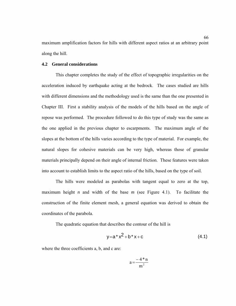
66

maximum amplification factors for hills with different aspect ratios at an arbitrary point

along the hill.

4.2 General considerations

This chapter completes the study of the effect of topographic irregularities on the

acceleration induced by earthquake acting at the bedrock. The cases studied are hills

with different dimensions and the methodology used is the same than the one presented in

Chapter III. First a stability analysis of the models of the hills based on the angle of

repose was performed. The procedure followed to do this type of study was the same as

the one applied in the previous chapter to escarpments. The maximum angle of the

slopes at the bottom of the hills varies according to the type of material. For example, the

natural slopes for cohesive materials can be very high, whereas those of granular

materials principally depend on their angle of internal friction. These features were taken

into account to establish limits to the aspect ratio of the hills, based on the type of soil.

The hills were modeled as parabolas with tangent equal to zero at the top,

maximum height n and width of the base m (see Figure 4.1). To facilitate the

construction of the finite element mesh, a general equation was derived to obtain the

coordinates of the parabola.

The quadratic equation that describes the contour of the hill is

cx*b2x*ay ++= (4.1)

where the three coefficients a, b, and c are:

2mn*4a −

=

67

21

m)x*2m(n*4

b+

=

111 y

mx1

mx*n*4c +⎟

⎠⎞

⎜⎝⎛ +

−=

where (x1, y1) are the coordinates of the left point at the base of the hill (see Figure 4.1).

Figure 4.1 Parameters for the equation of the parabola

Knowing the points (x1, y1), the maximum height (n) and the length of the base

(m), the coordinates of the points in the FE mesh along the parabola were obtained with

equation 4.1 and a spreadsheet. To minimize the number of cases to be studied, the

dimension m was fixed to 400 ft, and the following four values of n were considered: n =

38 ft, n = 75 ft, n = 115 ft, and n = 225 ft. Only two cases for n = 225 ft were analyzed

due to the problem of the stability of the natural slope. The slopes corresponding to the

values of n and m listed before are 21°, 37°, 49° and 66°, respectively. The soil deposit

depth beneath the hill was taken equal to 100 ft and the lateral extension from the hill’s

toes to the borders was equal to 200 ft in all the cases. The properties of the soil used as

input are the following:

n

m

y

x

x1,y1

68

Unit weight γ = 125 pcf

Poisson’s ratio ν=0.35

Damping ratio ξ = 0.05

The selection of the soil material used in the study was based on the UBC-97

Code as discussed in Chapter III. Only four soil categories were used: SB, SC, SD and SE,

and the shear wave velocities employed were the average of the values used in the code

to separate the different types. Using the shear wave velocity, the soil’s unit weight and

equation 3.2, the Q4MESH program calculates internally the shear modulus. The curves

for the variation of the shear modulus and damping ratio as a function of shear strain

were selected by trying to match the average shear wave velocity obtained from the

UBC-97 code with a suitable curve available in the program QUAD4M.

In the same manner as done with the escarpment, two historic earthquakes scaled

to have a maximum acceleration of 0.1g were used. The accelerograms are those of the

El Centro and San Salvador earthquakes. According to the objective of the study, only

the most critical cases were tabulated and are presented here. The finite element models

were always evaluated with both earthquakes to obtain the maximum amplification. The

final results presented here for the models of the hills with n = 38 and 225 ft were

obtained using the El Centro earthquake whereas those for the models with n = 75 and

115 ft were calculated with the San Salvador earthquake.

69

4.3 Ridge amplification results

This section present the results of the different cases and configurations of hills

examined. The effect of the different soil types and the two earthquakes on the

amplification of the acceleration signal at the hill’s surface is studied. The finite element

models analyzed are those illustrated in Figures 2.7 and 2.8 (section 2.6). By varying the

height of the hill four meshes were generated. These models were evaluated using the

finite element program QUAD4M. The results of the seismic analysis are displayed in

graphical form, as a plot of the peak acceleration along the hill and horizontal free

surface. At the end of this section the maximum amplification factors found as the

function of the height of the hill and the type of soil profile are presented.

The results of the study reported here are based on a horizontal soil deposit and

hill made up of only one type of material. Figure 4.2 shows the nodes of the finite

element model at the surface where the acceleration was calculated. In the following

subsections, the presentation of the results is divided according to the height of hill. The

graphs presented next are the most critical cases for each model. Therefore, in some

cases the seismic input is the El Centro earthquake and in other models the results

presented are those for the San Salvador ground motion.

Finally, the results of the study agree quantitatively with those of other studies

previously mentioned. They indicate that the amplification increases from the base to the

top of the hill.

70

Figure 4.2 Nodes at the surface of the model of the hill

Hill with height n = 38 ft

Figure 4.3 presents the peak acceleration obtained for a hill with a total height of

38 ft and aspect ratio n/m = 0.095. These results were obtained considering that the

combined soil system consists of a SE material or clay and using the El Centro

earthquake. The plot shows how the peak ground acceleration changes due to the

presence of the irregularity. The maximum values occur at the top of the hill and near the

boundaries of the model. The maximum amplification factor for this case is 1.53.

Figure 4.3 Peak ground acceleration for a hill with n = 38 ft

0

0.04

0.08

0.12

0.16

0.2

0 100 200 300 400 500 600 700 800 900


Pea

k A

ccel

erat

ion

(%)

El Centro Earthquake, A.F.=1.53

71

Hill with height n = 75 ft In this subsection the height of the hill was doubled with respect to the previous

case. The San Salvador earthquake was selected to generate the numerical results

because it produced higher values of amplification for this hill. This case was evaluated

for the four soil types and it was found that the SE material (or clay) produces higher

accelerations. Therefore, the curve in Figure 4.4 is for this material. The maximum

value of the absolute acceleration occurred at the top of the hill and is approximately

equal to 0.22g. The points at the base of the hill actually show deamplification although

not very significant: the peak acceleration is slightly less than 0.1g. According to the

graph, the maximum amplification ratio at the top with respect to the toe of the hill is

2.34.


0

0.05

0.1

0.15

0.2

0.25

0 100 200 300 400 500 600 700 800 900


Pea

k A

ccel

erat

ion

(%)

San Salvador Earthquake, A.F.=2.34

72

To gain further insight into the behavior of the soil system and to verify the small

deamplification observed, a model of the soil deposit without a hill is presented next.

The dimensions of the soil deposit are equivalent to the model with a hill of n = 75 ft.

The horizontal extension of the soil deposit is 800 ft and its depth is 175 ft, i.e. the same

as the total height of the previous model. Figure 4.5 presents the results for a SE material

and the San Salvador earthquake. As it was expected, the plot shows that the peak

acceleration is constant when no irregularities are present. The graph shows that the

value of the deamplification at the top of the soil deposit agrees very well with the results

at the toe of the hill in the previous case (Figure 4.4).

Figure 4.5 Peak acceleration at the top of a soil deposit without irregularities


This case was also evaluated for the different soils and the two earthquakes.

However, the SE material and the San Salvador earthquake yielded higher accelerations.

0.09

0.1

0.11

0.12

0 100 200 300 400 500 600 700 800 900


Pea

k A

ccel

erat

ion

(%)

San Salvador Earthquake, SE material

73

The results are presented in Figure 4.6 and they show that there is an amplification of the

acceleration along the surface of the hill. The maximum amplification ratio is 1.60.



This model was only evaluated for two soil profiles: SB and SE. The soils

classified as SC and SD, granular materials, are not able to maintain stability at this slope,

and for this reason they were not considered. The variation of the peak acceleration for a

SB soil and the scaled El Centro earthquake (the most critical one) is presented in Figure

4.7. At the very top of the hill there is an amplification of 2.35 times the acceleration at

the toe of the hill.

0

0.05

0.1

0.15

0.2

0.25

0 100 200 300 400 500 600 700 800 900


Pea

k A

ccel

erat

ion

(%)

San Salvador Earthquake, A.F.=1.60

74


General comments

It is important to note that all the plots previously presented are only examples of

many cases evaluated. The next table summarizes the amplification factors obtained

using the four models with different heights of the hill and the four types of materials.

The amplification factors are defined as the ratio between the maximum acceleration at

the surface of the hill with respect to the peak acceleration at the toe of the hill. The

maximum value of the surface acceleration for all the cases examined was nearly 0.22g

and it occurred in the n = 75 ft model. The maximum amplification factor is 2.35 and it

was obtained for the n = 225 ft model.

Table 4.1 Maximum Amplification Factors for the Hill

0

0.04

0.08

0.12

0.16

0.2

0.24

0 100 200 300 400 500 600 700 800 900


Pea

k A

ccel

erat

ion

(%)

El Centro Earthquake, A.F.=2.35

n (ft) n/m SB SC SD SE

38 95/1000 1.01 1.52 1.46 1.5375 188/1000 1.34 1.93 2.16 2.34115 288/1000 1.48 1.47 1.60225 563/1000 2.35 0.90

Soil Classification (UBC - 97)

75

4.4 A general equation for the amplification factors

Table 4.1 can be used to estimate the maximum amplification factors expected on

hills with four different aspect ratios n/m and a homogeneous soil. It is recommended to

interpolate the values of the table for cases not covered there but reasonably close. To

evaluate other models that cannot be associated to the cases presented in the table of the

previous section, in this section we evaluate a special case to generate a general equation.

With this equation the user can obtain the amplification factor for hills with any aspect

ratio within a certain range. The procedure followed to derive the equation is very

similar to the one followed for the case of the escarpment. The resulting equation is a

function of the ratio between the height, and the width of the hill and the location of the

point, defined as a fraction of height of the ridge. The validity of the equation and thus

the amplification factors is limited to values of n/m from 0.095 to 0.56. The equation was

derived for a soil deposit-hill system formed by two different materials for the deposit

and for the hill. Figure 4.8 shows the parameters involved in the case studied.

Figure 4.8 Parameters identification

n

m

y

Vs1

Vs2

76

The shear wave velocities were taken equal to Vs1 = 575 ft/s and Vs2 = 1850 ft/s,

whose values correspond to soil profiles SE and SC according to the UBC-97

classification. Table 4.2 presents the amplification factors calculated using heights with n

equal to 38, 75, 115 and 225 ft at different elevations expressed as percent of the total

height of the hill.

Table 4.2 Amplification Factors for Hills of Different Heights

The procedure to determine the formula sought begins by plotting the

amplification factors as a fraction of the height of the hill for each model defined by its

ratio n/m. This is illustrated in Figure 4.9 for a hill with height/width ratio of 95/1000.

The graph suggests that a cubic equation could be used to represent reasonably well the

general pattern. Therefore, a cubic equation of the form

ii2

i3

i D*C*B*A.F.A +α+α+α=

y 38 75 115 2250n 1.00 1.00 1.00 1.00

0.22n 1.19 1.32 1.00 1.050.38n 1.32 1.93 1.27 1.330.55n 1.49 2.50 1.59 0.880.67n 1.71 2.42 1.61 0.710.77n 1.84 2.42 1.63 0.920.84n 2.03 2.60 1.77 1.090.91n 2.14 2.72 1.89 1.28

n 2.87 2.85 2.08 1.50

Amplification Factor (m = 400 ft)n (ft)

77

was derived for each of the four hills with different ratio n/m.

Figure 4.9 An example of a cubic trendline for n/m = 0.095

A mathematical procedure similar to that discussed in Chapter III was used to

obtain the appropriate coefficients of a general equation, also a cubic polynomial, which

must be able to cover the four cases. Equation 4.2 is the resulting formula that provides

the amplification factor (A.F.) for hills with height-to-width ratios from 95/1000 to

563/1000.

432

23

1 a*a*a*a.F.A +α+α+α= (4.2)

where:

257.15r*012.163r*294.499r*043.423a 231 +−+−=

454.10r*593.82r*400.158r*404.33a 23

2 −+−=

518.4r*964.105r*780.456r*585.516a 233 −+−=

127.1r*283.2r*491.8r*724.8a 23

4 +−+−=

0.00

0.50

1.00

1.50

2.00

2.50

3.00

3.50

0 0.2 0.4 0.6 0.8 1 1.2

Fraction of height of ridge

Am

plifi

catio

n Fa

ctor

78

:m/nr = ratio between the height and width of the base of the hill

α = fraction of height of hill

Figure 4.10 compares the curve obtained with the proposed equation (4.2) and

with the original best-fit cubic curve passing through the data points. The latter is the

same curve presented in Figure 4.8. Figure 4.10 highlights the accuracy of the proposed

general equation.

Figure 4.10 The cubic trendline and the general equation for n/m = 0.095

4.5 Frequency analysis

According to the previous works discussed on Chapter I and the results obtained

from the escarpment analysis, it was expected that, as the elevation of the irregularity

increases, so do the acceleration. However, this was not necessarily the case in the study

of hills. As an example, the peak surface acceleration for hills with n = 38 ft and n = 75

ft are compared in Figure 4.11, where the difference with the previous patterns are

0.000

0.500

1.000

1.500

2.000

2.500

3.000

0 0.2 0.4 0.6 0.8 1

Fraction of height of escarpment

Am

plifi

catio

n fa

ctor

Cubic Proposed

79

evident. Note that at the top of the hill a greater peak acceleration was obtained for the

case of n = 38 ft, i.e. for the lower hill.

Figure 4.11 Comparison of ridge amplification subjected to El Centro earthquake

The results in Figure 4.11 are for the case where El Centro earthquake was

applied. It is noted that when the San Salvador earthquake is used as input, the results

obtained are those expected. Two types of soils were used in the case of Figure 4.11: a

soil SC for the bottom deposit and a soil SE for the hill. Explaining the reasons for this

behavior requires looking at the amplification problem from another point of view. The

cause may be related to the frequency content of the earthquake compared to the natural

frequencies of the soil deposit. If some of the frequencies of the dominant components of

the seismic motion coincide with a lower frequency of the soil deposit, the seismic waves

will be further amplified.

To check whether the explanation for the results in Figure 4.11 are due to a

resonant-like condition, the case of a hill with height n = 38 ft was evaluated using the El

0

0.05

0.1

0.15

0.2

0.25

0.3

0.35

0 100 200 300 400 500 600 700 800 900


Pea

k A

ccel

erat

ion

(%)

n/m=95/1000 n/m=188/1000

80

Centro ground motion and two soil profiles: a material type SC and next a type SE soil.

The natural frequencies of the soil deposit-hill system were calculated using a finite

element program for two-dimensional problems written in FORTRAN (Arroyo 1997).

The reason for switching programs is that the program QUAD4M does not compute the

natural frequencies of the soil system. The results of the frequency analysis were the

following. The soil system with a SC material has a fundamental frequency of 25.27 rad/s

whereas the frequency diminishes to 7.85 rad/s for the SE material. The frequency

spectrum of the El Centro earthquake shows many peaks since it corresponds to a typical

broad band signal. However, the relative importance of the lower frequencies produces

more amplification in the n = 38 ft case.

Because of the interdependence between the fundamental frequency of the soil

deposit-hill system and the frequency content of the earthquake in the amplification

obtained, it was necessary to determine for each case which one is the most severe

earthquake. Only this earthquake was used to calculate the amplification factors for the

different hills. Table 4.3 summarizes the earthquake used to analyze each of the hills

with different heights.

Table 4.3 Most Severe Seismic Motions for the Analysis

Height of hill n height/width ratio Earthquake(ft) n/m38 95/1000 El Centro75 188/1000 San Salvador115 288/1000 San Salvador225 563/1000 El Centro

81

4.6 Summary

This chapter presented a dynamic finite element analysis of different models of

soil deposit-hill systems to calculate the peak acceleration at the surface nodes. The

pattern of results observed indicate that there is amplification along the hill in all the

cases. All the cases except the one for a hill of height n = 38 ft shows a deamplification of

the absolute acceleration at the toe of the hill. Table 4.4 shows a summary of the highest

amplification factors for the different hill geometries regardless of the type of soil

material. To obtain these values, all the material types were considered, with the

exception of the SC and SD soils in some cases. As it was cited before, for n = 225 ft

these granular materials do not exhibit stability for hills with aspect ratio of 563/1000 or

higher. For an unfavorable combination of soil types, a general formula that yields the

amplification factor at different elevations along the hill was derived. The formula is

rigorously valid for hills with aspect ratio n/m from 95/1000 to 563/1000. Hills with

lower height-to-width ratios show negligible amplifications. Hills with values of n/m

higher than 0.563 are not likely to be the site of residences.

Table 4.4 Summary of Maximum Amplification Factors for Different Hills

n (ft) n/m Amplification Factors38 95/1000 1.5375 188/1000 2.34115 288/1000 1.60225 563/1000 2.35

82

Chapter V

A Case Study in Puerto Rico

5.1 Introduction

The effects of surface topography on the seismic ground response have been

subjected to numerous studies during the last two decades. The present study and others

mentioned in Chapter I verified via numerical simulation the amplification in the ground

accelerations due to surface irregularities. This phenomenon has been observed in the

field several times, especially in countries such as Italy or Greece, in which there are

many seismic regions with an irregular topography. Because of its unique geography,

also in Puerto Rico have many regions prone to experience topographic seismic

amplification.

The objective of this research is to perform a parametric study to account for the

amplification of seismic waves in hills and escarpments. The final goal is to come up

with a simple methodology to account for this effect in the seismic codes. Chapter III

and Chapter IV examined the effects of two irregularities with idealized geometries on

the amplification for two earthquakes with distinct characteristics. In this chapter a case

study of potential topographic amplification in Puerto Rico will be described and

analyzed. This real case differs from the ideal models used in the previous two chapters.

The geometry of the irregularity is rather complex and so is the soil profile at the site

under study. To define them, it was necessary to use topographic maps as well as site

inspections to take soil samples for laboratory testing. Moreover, an artificial earthquake

83

especially generated for the south of Puerto Rico was used as seismic input, instead of the

historical earthquakes used previously.

5.2 Geographic conditions of Puerto Rico

Puerto Rico is part of the Greater Antilles Island chain in the Caribbean Sea. It

lies approximately 100 miles south of the Puerto Rico Trench, a depression of the ocean

floor that reaches depths of 30,249 feet, the deepest depth known in the Atlantic Ocean.

The Island has an approximate rectangular shape that extends about 110 miles from east

to west and 40 miles from north to south. The island has a high population density that

reached 3.8 million inhabitants in the year 2000. Puerto Rico is a mountainous island

with central highland areas that rise to a maximum altitude of about 4,400 feet above sea

level. The Cordillera Central, the Sierra de Luquillo, and the Sierra de Cayey are

generally oriented east-west and dominate the mountainous southern two-thirds of the

island, as illustrated in Figure 5.1. An area of gently dipping limestone that has been

deeply dissected by dissolution forms a wide band of karst topography along most of the

north. Flat-lying coastal plains and alluvial valleys compose a discontinuous belt around

much of the periphery of the island. The coastal plain is especially prominent along part

of the south coast where adjacent streams to form a broad, continuous plain (USGS 1997)

deposited coalescing fan deltas.

84

Figure 5.1 Topographic view of Puerto Rico (Rivera 1995)

Clearly, the geography of Puerto Rico, along with the social and economic

conditions that affect the population distribution, makes a study of the topographic

amplification worthwhile in many regions of the Island. For example, Figure 5.2 shows a

typical view of residential structures located on hills and slopes where topographic site

effects can exacerbate the consequences of a strong earthquake. The picture was taken in

Yauco near the city of Ponce at the south of the island.

85

Figure 5.2 Residences located on the hill

5.3 Site location

A review of the topographic maps of Puerto Rico, indicates that there are many

regions that may be prone to seismic amplification due to topographic irregularities. An

area near the town of Guánica, in the south of the Island was chosen for study. The town

of Guánica is indicated within an ellipse in Figure 5.3. Near this town there are

numerous hills surrounded by the flat land of the Valle de Lajas.

Figure 5.3 Map of the municipalities of Puerto Rico showing the location of Guánica

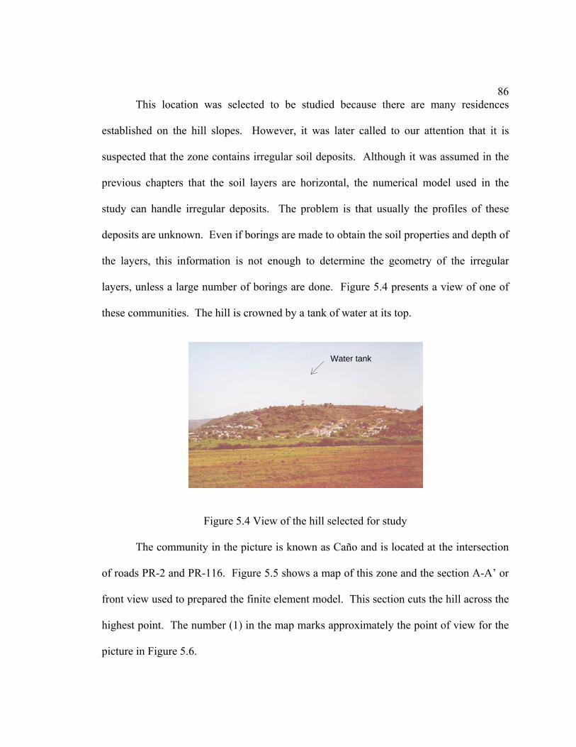
86

This location was selected to be studied because there are many residences

established on the hill slopes. However, it was later called to our attention that it is

suspected that the zone contains irregular soil deposits. Although it was assumed in the

previous chapters that the soil layers are horizontal, the numerical model used in the

study can handle irregular deposits. The problem is that usually the profiles of these

deposits are unknown. Even if borings are made to obtain the soil properties and depth of

the layers, this information is not enough to determine the geometry of the irregular

layers, unless a large number of borings are done. Figure 5.4 presents a view of one of

these communities. The hill is crowned by a tank of water at its top.

Figure 5.4 View of the hill selected for study

The community in the picture is known as Caño and is located at the intersection

of roads PR-2 and PR-116. Figure 5.5 shows a map of this zone and the section A-A’ or

front view used to prepared the finite element model. This section cuts the hill across the

highest point. The number (1) in the map marks approximately the point of view for the

picture in Figure 5.6.

Water tank

88

Figure 5.6 View from road PR 116 of Caño Hill

5.4 Study of soils at the site

After selecting the area of study, an intensive search was conducted to identify the

soil profile for the Caño hill. Opposed to other models previously studied, in which a

homogeneous soil profile was used, this case required use of a stratified profile. To

evaluate the site conditions a visual inspection was conducted and simple laboratory tests

were prepared. In addition, the soils were identified with the help of the maps of the

National Soil Survey. During the field visit a number of samples of soils at different

elevations of the hill were collected. Those samples presented different textures and

colors. The soil samples were tested in the geotechnical laboratory of the Civil

Engineering and Surveying Department of UPR-M. The tests of Liquid Limit, Plastic

Limit, moisture content were carried out and the unit weight was obtained. Once these

characteristics were available, it was possible to identify the soils according to the UBC

89

97 classification and the proper materials curves available in the Q4MESH computer

program were selected. To verify these properties, the soils in the region of Caño were

also evaluated according to a soil map prepared by the National Soil Survey (USDA

1963). Figure 5.7 shows a soil map of the Valle de Lajas Area with the soils identified

with letters and numbers. The first capital letter is the initial of the soil name. The

second capital letter shows the slope and the final number (2) indicates that the soil is

eroded.

The soil profile of the Caño Hill consists of five types of materials. These types

vary from clay to gravel. In turn, the clay types vary in unit weight and in their plasticity

indices. The hill and the surrounding valley consist mostly of clay, but the top of the hill

is composed of rock fragments, limestone and other dense materials. Table 5.1

summarized the properties of the materials analyzed: unit weight γ, shear wave velocity

VS in ft/s, Poisson’s ratio ν, and damping ratio ξ.

Table 5.1 Materials Properties for the Model of the Caño Hill

Material Identification γ (pcf) VS (ft/s) ν ξDense soil and soft rock 125 1850 0.35 0.05

Clay 90 900 0.35 0.05Clay 100 900 0.35 0.05

High plasticity Clay 90 575 0.35 0.05Dense soil and soft rock 100 1850 0.35 0.05

91

5.5 Seismic excitation

It is known that the crust of the Earth consists of approximately twelve tectonics

plates. The relative movements of the borders of those plates produce

different kinds of earthquakes. The seismic risk of Puerto Rico is due to the fact that it is

located between the plates of the Caribbean and North America, as illustrated in Figure

5.8.

Figure 5.8 Seismic activity in America and Caribbean (Yeats et al 1997)

92

Hence, Puerto Rico is located in an active seismic zone that extends from

America Central to Venezuela and is classified by the UBC 97 as seismic zone 3. The

history of Puerto Rico has witnessed several strong earthquakes that occasioned serious

damages. Those earthquakes occurred in times where the majority of building

constructions was in timber and the population was scarce compared to present levels.

The damages that a strong seismic event can cause nowadays are much greater than in the

past, due to the population increase and the many constructions vulnerable to ground

motions.

Puerto Rico suffered four strong earthquakes since the colonization by the

Spaniards. The most recent one occurred on October 11, 1918, and its epicenter was

located at the northwest of the Island. The magnitude of that earthquake is estimated to

have been approximately 7.5 in the Richter scale. The damages were restricted

principally to the west region due to the proximity to the epicenter. The consequences of

the event were 116 deaths and millions of dollars of losses. Many residential

constructions, public buildings, bridges and other edification suffered significant damage.

Other strong earthquakes affected the Island in 1867, 1787 and 1670, but the data about

them is scant.

The study presented in Chapter III and IV used two historical earthquakes as

seismic input, namely the El Centro and San Salvador. In this part of the research we

will evaluate a case study of topographic amplification in Puerto Rico. Therefore, we

decided to use as input applied at the rigid base rock an artificial accelerogram

compatible with a new design spectrum recommended for Puerto Rico in a recent study

93

(Irizarry 1999). The study, conducted at the Civil Engineering and Surveying

Department of UPR-M, defined ground design spectra for four cities in the Island and a

sample of artificial accelerograms compatible with the spectra. The seismic excitation

used as input motion for the finite element model was scaled to 0.3g. Table 5.2 shows

the main characteristics of the original accelerogram from the study mentioned. Also,

Figure 5.9 illustrates the acceleration time history and Fourier spectrum for the

accelerogram.

Table 5.2 Characteristics of an Artificial Earthquake for Puerto Rico

Duration

(secs)

Peak

Displacement

(cm)

Peak Velocity

(cm/s)

Peak

Acceleration

(cm/s2)

10.02 11.78 55.25 -451.26

(a)

0 1 2 3 4 5 6 7 8 9 10

-0.25

-0.2

-0.15

-0.1

-0.05

0

0.05

0.1

0.15

0.2

0.25

Time [sec]

Acc

eler

atio

n [%

g]

94

(b)

Figure 5.9 Acceleration time history (a) and Fourier Spectrum (b) of the artificial earthquake

5.6 The finite element model

As mentioned previously, this chapter presents the topographic amplification

study of a real case, i.e. a hill located in Guánica, P.R. The hill and the underlying soil

deposit were discretized with finite elements using the QUAD4M program. Unlike the

configurations analyzed in previous chapters where the hills were described by perfect

curves, in this study a topographic map was used to evaluate the real natural elevations

from the sea level. Figure 5.6 (section 5.2.1) presents a view of the hill to be studied

from road PR 116. The map in Figure 5.5 shows the section studied and the location

from where the photo in Figure 5.6 was taken.

Figure 5.10 displays the 2-D finite element mesh generated for the Caño Hill.

The model has 539 elements, 584 nodes and a total of 1168 degrees of freedom. The

0 10 20 30 40 50 60 700

500

1000

1500

2000

2500

3000

3500

4000

Frequency [rad/sec]

Am

plitu

de

95

figure shows the different elevations taken from the map and the valley surrounding the

hill. The maximum elevation was 344 ft with respect to the level of the ground surface

(see Figure 5.11). The extension of the plains at both sides was 2952 ft. The figure also

shows the boundary conditions used at the bottom and sides of the model. The bedrock is

considered to begin at the location of the fixed nodes at the bottom.

Figure 5.10 Finite element mesh for the Caño Hill

5.7 Results of the numerical simulation

This section presents the results of the numerical simulation of the topographic

amplification problem. It must be pointed out that this case differs from the theoretical

cases studied in Chapter IV. In the previous chapter, the materials at the site were

assumed to be homogeneous and the ridge was considered to be isolated. In this case,

however, the soil profile is quite different from a simple homogeneous halfspace and

different kinds of materials are used in the FE model. Also, the Caño Hill cross section

has three different heaps and thus it is not an isolated hill as in the cases studied in

Chapter IV. Figure 5.11 displays the coordinates for the mesh generated. The horizontal

coordinates in this figure will help in the interpretation of the results to be presented next.

96

These more general types of topographic feature present additional scattering and

diffraction of seismic waves and there could be amplification or deamplification of the

seismic motion depending on the point considered. This can be clearly seen from the

graph of the peak accelerations presented in Figure 5.12. The plot shows the peak

acceleration at all the surface nodes of the model. The results in Figure 5.12 are peculiar

in the sense that the maximum amplification not necessarily occurs at the top of the hills.

Actually the highest amplification occurs at the valley on the right side of the mesh, and

at an elevation of 40% of the maximum height of the hill. There are many points or

nodes that present a deamplification, in particular those at the tops of the hills where the

material type is gravelly with limestone fragments. The materials where amplification

occurs are either cohesive materials or different types of clays.

Figure 5.11 Coordinates for the Caño Hill mesh

97

Figure 5.12 Acceleration results for Caño Hill

It is known that the seismic waves are amplified on sites where the soil deposits

are soft and with significant thickness. Those areas generally include alluvial valleys and

zones of drained ponds and lakes. During an earthquake, those sites shake with more

intensity and for more time. It is important to mention that Caño Hill is located beside a

river. Indeed, the valley is part of a river basin.

To generate and tabulate the amplification factors for this local topography, it was

necessary to calculate average values of the peak acceleration at all the points at a given

elevation. The reason for presenting the results in this form is because the mesh is not

symmetrical and the surface acceleration obtained is not equal for all the points at a same

elevation. Figure 5.13 presents the variation of the average peak acceleration with

respect to the fraction of the hill’s height. It is recalled that the seismic motion applied at

the bedrock has a PGA = 0.3g. Finally, Table 5.3 illustrates the amplification or

deamplification factors depending on the elevation considered.

0

0.1

0.2

0.3

0.4

0.5

0.6

-4000 -2000 0 2000 4000 6000 8000 10000 12000


Pea

k A

ccel

erat

ion

(%)

98

Figure 5.13 Average acceleration at different elevation

Table 5.3 Amplification and Deamplification Factors

The next two figures show the distribution of stresses and accelerations in the full

mesh predicted by QUAD4M and plotted using the program Q4MESH. Figure 5.14

illustrates the shear stress distribution where the maximum value is represented by a red

color with a value of 4753 psf and the minimum values are represented by a blue color

0

0.2

0.4

0.6

0.8

1

1.2

0 0.1 0.2 0.3 0.4 0.5

Average Acceleration (g)

Frac

tion

of H

eigh

t

Fraction of Amplification Deamplification Height of Hill Factor Factor

0.05h 1.000.14h 1.150.29h 1.460.43h 0.910.55h 0.630.62h 0.490.71h 0.450.76h 0.420.81h 0.490.9h 0.350.95h 0.40

h 0.42

99

with a value of 151.4 psf. The figure shows that the maximum stresses occur at the base

of the model.

Figure 5.14 Stress distribution

Figure 5.15 illustrates the distribution of peak accelerations over the model. The

range of values goes from 0.07 to 0.48 g. Here again, the red color and the blue color

represent the maximum and minimum values, respectively. The minimum values are at

the top of the hill where the material type is cohesionless with fragment of rocks. On the

contrary, the maximum accelerations are found at the toe of the hill, where the majority

of the residential structures are located.

Figure 5.15 Acceleration distribution

100

5.8 Comparison with the proposed simplified methodology

It is interesting to compare the results of the Caño hills with those from the

general amplification formula and the data in the table generated in Chapter IV for ideal

hill cases. To use the table or formula, we need to know the ratio between the height of

the hill and the length of its base. For the Caño hills a ratio of 0.095 was used to

calculate the amplification factors. According to Table 5.3, the amplification factor at

14% of the maximum height is 1.15, whereas the equivalent result with the proposed

equation at the same elevation is 1.17. At 29% of the height, the real case (i.e., the study

done in this chapter) shows an amplification of 1.46, while the proposed equation

predicts an amplification factor of 1.28. If we calculate an amplification factor as the

average value of the amplification factors for the four materials and for n/m = 0.095, we

obtain 1.38. It is important to have in mind that the proposed general equation was

derived using only two types of soil materials and the amplification factors listed in Table

4.1 of Chapter IV were generated for soil deposits and hills of uniform materials.

Therefore, the results obtained with the methodology of Chapter V are acceptable

considering the differences in the material profiles and the complicated geometry of the

real case studied.

5.9 Summary and final comments

In this chapter a real case of topographic amplification was described and studied

in detail. The hill or group of hills analyzed is located in Guánica, Puerto Rico. The

conditions of the surface topography are very particular. Firstly, an extended valley or

101

plain surrounds the hill, beside the toe of the hill there exists a river and the soil material

of the zone is not homogeneous. The soils consist of clays with different plasticity

indexes, and the top of the hill consists of a cohesionless material with rock fragments.

Because of these characteristics, the results do not follow the same trend than in the

theoretical cases studied in the previous chapter. In particular, the types of materials play

an important role in this kind of analysis. Nevertheless, the numerical simulation done

with the finite element program showed that there is significant amplification.

The amplification factors predicted with the formula and table presented in

Chapter IV were compared with those of the real case of the Caño hills. The accuracy of

the results obtained with the proposed simplified methodology is acceptable, given the

vast differences in geometry and material composition between the idealized cases used

to derive the formula and table and the actual site studied.

In closing, it is important to underscore that in the case of the Caño community

the highest amplification occurred at almost 0.3 of the maximum height of the hill. This

indicates that there is a clear and present danger in the event of a severe earthquake: the

majority of the residential structures are located at about this elevation. To compound the

problem, many of the houses have slender columns with the rooms located in the second

floor. In fact, they are cases of cantilevered-column building systems, structural

configurations that are particularly vulnerable to seismic motions. The study of the

seismic response these residential structures will be the object of a future investigation.

102

Chapter VI

Conclusions and Recommendations

6.1 Summary and conclusions

This thesis presented a numerical study of the phenomenon known as

“topographic amplification” of the seismic waves. The seismic response of interest was

the absolute acceleration at the free surface of the topographic irregularities. Two

irregularities were studied: an escarpment or embankment and a hill or ridge, both

considered as 2-dimensional, i.e. their profile is the same in any cross-section parallel to

the plane of analysis. Two acceleration time histories of past earthquakes with different

characteristics, the 1940 El Centro and the 1986 San Salvador earthquakes, were used as

excitation. Both accelerogram were scaled so that their peak ground acceleration is 0.1g.

The finite element method was used for modeling the soil system and calculating the

response of the topographic irregularities when they were subjected to a seismic motion

at the underlying bedrock. The program QUAD4M was used along with the interface

program Q4MESH to generate the required finite element meshes. The QUAD4M

program considers in an approximate way the nonlinear behavior of the soil deposits

when they are subjected to severe earthquakes. This is done by means of the Equivalent

Linear Method.

The results obtained for the cases of escarpments indicate that there is an increase

in the ground acceleration as one moves up along the surface of the slope compared to the

original acceleration at the bedrock. In the escarpment analyses, the material type

103

defined as SC in the UBC-97 classification causes the largest amplification. Also, the

studies indicate that the amplification ratios between the top and base were greater for El

Centro earthquake than for the San Salvador earthquake. However, the San Salvador

produced higher peak accelerations in absolute terms.

The models of the hills showed greater amplification factors than the

escarpment’s models. The maximum acceleration for a hill was found when a model

with height n=75 ft was used. However, the maximum amplification factor was obtained

in the hill with height n=225 ft. In the case of the hills a phenomenon not observed in the

escarpment occurred. All the hill cases but one exhibited a deamplification at the toe of

the hill.

The maximum amplification factors were presented in tables and they range from

1.00 to 2.35. Not all the soils in the UBC-97 classification were always used because in

some cases the materials did not exhibit stability for the more pronounced slopes.

In theory, the topographic amplification is strictly caused by the discontinuity in

the geometry of the soil deposit. The diffraction of the seismic waves as well as the

multiple reflections within the boundaries of the irregularity are usually thought to be

responsible for the amplification. Therefore, in principle, the type of material is not

relevant for this problem. However, one of the first peculiarities of the phenomenon that

was observed during the course of the study was that the type of soil material does play

an important role in the occurrence of amplification. Therefore, it was decided that each

model of the soil deposit-hill and soil deposit-escarpment system needed to be analyzed

using different types of soils. The classification provided in the UBC-97 code, adopted in

104

Puerto Rico, was used to select the soil types. There are six soil types in the UBC-97.

Out of these six types, the soils referred to as SA and SF were not used. The type SA is a

very hard rock typical of some regions in the Eastern US and thus it was considered that

it would not represent the situation in Puerto Rico. The soil profile SF requires, according

to the code, site-specific geotechnical studies and thus the general character of the study

carried out here would no be useful for this kind of material. Therefore, only the soils

classified as SB, SC, SD and SE were considered. In some models it was assumed that the

same material formed the escarpment and hill as well as the soil deposit underneath. In

other models, a combination of two different soils that was shown to be unfavorable, i.e.

that leads to higher amplification, was used.

The amplification studies presented in Chapters IV and V are based on highly

idealized geometries of the topographic irregularities. To observe the situation in an

actual case, a site at the south of Puerto Rico in the municipality of Guánica was selected

for a detailed analysis. Using the best data available from maps and site visits, a finite

element model of the cross-section of a group of hills was created. In order to further

enhance the real character of the analysis, a synthetic earthquake specifically developed

for the south of Puerto Rico in a previous study was used as seismic input. The case was

complicated not only because of its geometry but also due to the fact that the soil profiles

at the site were not similar to those studied before. For instance, the valley at the bottom

of one of the hills is near a river basin. The results were interesting because the

maximum amplification did not happen at the top of the hill, but at about 0.3 of the

maximum height. This can pose a problem to the many residential structures built at this

105

elevation. Although the geometry and materials of this real case are quite different from

those considered in the previous chapters, when the tables and general formula developed

therein are applied, they produce reasonable results.

6.2 Suggestions for further studies

Although this work tried to be as comprehensive as possible, there are a number

of topics that were not addressed because of time limitations. It is believed that these

topics are worth, at least, a closer look. They are listed below in no specific order.

1. The same methodology used in this thesis can be applied to study hills with

shapes different than the parabolic case considered here. In addition, the 3-

dimensional effect that may occur in canyons is worth studying.

2. If one can find seismic records recorded at the field, both away from the

topographic irregularity and also on its surface and on the hill or escarpment

itself, they can be very useful to validate the numerical simulation study. In

this case, it is necessary to know at least in an approximate way the properties

of the soil profiles where the accelerogram were collected.

3. Although in this study a case of topographic amplification using real field data

and geometry was used, it is interesting to perform more of these analyses for

other sites in Puerto Rico.

4. The study undertaken here focused on one of the horizontal components of the

earthquake. This was done because, in general, they are the strongest

106

components and those that affect the most the buildings and other structures.

However, it is recommended to extend the analysis so that the vertical

components of the ground motions are also included.

5. The curves in the program QUAD4M that describe the variation of the shear

modulus G and the damping ratio ξ as a function of the shear strain are

limited to a few options. These curves are required by the Equivalent Linear

Method to take into account the nonlinear behavior of the soil under a strong

ground motion. The user is forced to adopt one of the curves that better

matches the material for the case under study. This is not a problem if one can

choose among a variety of curves, but as mentioned before, the options are

limited. If it is possible to incorporate more options to the library of curves of

the program, it will enhance the applicability of the computer program.

6. Two features of the topographic amplification phenomenon were not studied

in this thesis: the possible increase in the duration of the accelerogram and the

occurrence of differential motions along different points on the surface of the

irregularities. These effects should be examined because, even though the

most threatening result of the terrain irregularities is the amplification of the

ground acceleration, they may be also be detrimental for certain structures.

7. The San Salvador and El Centro earthquakes used in the parametric study

were selected because they represent two seismic motions with opposite

characteristics. However, if one wants to increase the confidence in the

107

amplification factors recommended, the use of more earthquakes will always

be of help.

108

References

1. Abramson, L.W., Lee, T.S., Sharma, S., and Boyce G.M. 1996. Slope Stability and Stabilization Methods. John Wiley & Sons, New York.

2. Arroyo, J. R. 1997. “UPRSOIL, a computer program”. Civil Engineering

Department, University of Puerto Rico, Mayagüez, P.R. 3. Arroyo, J. R. 1999. Nonlinear Seismic Response of Stratified Soil Deposits Using

Higher Order Frequency Response Functions in the Frequency Domain. Ph.D. Thesis. Civil Engineering Department, University of Puerto Rico, Mayagüez, P.R.

4. Athanasopoulos, G. A. and Zervas C. S. 1993. Effects of Ridge-Like Surface

Topography on Seismic Site Response. Soil Dynamics and Earthquake Engineering VI, Computational Mechanics Publications, Boston, Massachussets. 3-18.

5. Bouchon, M. 1973. Effect of Topographic on Surface Motions. Bulletin of the

Seismological Society of America. 63(3): 615-632. 6. Castellani, A., Peano A. and Sardella, L. 1982. Seismic Response of Topographic

Irregularities. Third International Earthquake Microzonation Conference Proceedings, Seattle, Washington, 2:533-540.

7. Cook, R. D., Malkus, D.S. and Plesha M. E. 1989. Concepts and Applications of

Finite Element Analysis. John Wiley & Sons, New York. 8. Geli, L., Bard, P. and Jullien, B. 1988. The Effect of Topographic on Earthquake

Ground Motion: A Review and New Results. Bulletin of the Seismological Society of America. 78(1):42-63.

9. Hudson, M., Idriss, I. M. and Beikae, M. 1994. “User's Manual for QUAD4M”,

Center for Geotechnical Modeling, University of California, Davis, California.

10. Idriss, I. M., Lysmer, J., Hwang, R. and Seed, H.B. 1973. “User's Manual for QUAD4”, College of Engineering, University of California, Berkeley, California.

11. Interactive Software Designs, Inc. 1995. Reference Manual, XSTABL-An Integrated

Slope Stability Analysis Program for Personal Computers, Version 5, Moscow, Idaho. 12. International Conference of Buildings Officials. 1997. Uniform Building Code 1997.

2, Chapter 16, Division V,Section 1636.2.6. Whittier, California.

109

13. Irizarry, J. 1999. Design Earthquake and Design Spectra for Puerto Rico’s Main

Cities based on Worldwide Strong Motion Records. MSCE Thesis, Civil Engineering Department, University of Puerto Rico, Mayagüez, P.R.

14. Kramer, S. L. 1996. Geothecnical Earthquake Engineering. Prentice-Hall, New

Jersey.

15. Peters, J. and Kala, R. 1999. “Users Guide to WinMesh”, United States Army Engineer Waterways Experiment Station, Vicksburg, Mississippi.

16. Rivera, M. 1995. Welcome to Puerto Rico. http://www.welcome.topuertorico.org,

updated February 2001. 17. Sanchez-Sesma, F. J. 1990. Elementary Solutions for Response of a Wedge-Shaped

Medium to Incident SH and SV Waves. Bulletin of the Seismological Society of America. 80(3):737-742.

18. Sanchez-Sesma, F. J. 1997. Strong Ground Motion and Site Effects. Computer

Analysis and Design of Earthquake Resistant Structures A Handbook. Computational Mechanics Publications, Southampton, UK, 3:201-239.

19. Sanchez-Sesma, F. J. and Campillo, M. 1993. Topographic Effects for Incident P,

SV and Rayleigh Waves. Tectonophysics, 218:113-125. 20. Sano, T. and Pugliese, A. 1999. Parametric Study on Topographic Effects in

Seismic Soil Amplification. Second International Symposium on Earthquake Resistant Engineering Structures. WIT Press, Ashurst, Southampton, UK. pp. 321-330.

21. Strong Motion Data Center, Department of Conservation, Mines & Geology. http://

www.consrv.ca.gov/dmg/csmip/index.htm, 1999. 22. Terzaghi, K., Peck, R. B., and Mesri, G. 1996. Soil Mechanics in Enginerring

Practice. John Wiley & Sons, New York. 23. U.S. Department of Agriculture, Soil Conservation Service. 1963. Soil map of Lajas

Valley Area, Puerto Rico. 24. U.S. Geological Survey. 1997. Ground water atlas of the United States, Segment 13.

Hydrologic Investigations Atlas 730-N, Reston, Virginia, p. N23. 25. Yeats, R. S., Sieh, K., and Allen, C. R. 1997. The Geology of Earthquakes. Oxford

University Press, New York.

topographic amplification of earthquakes in puerto rico

Documents