topological methods for nonlinear differential equations
TRANSCRIPT

TOPOLOGICAL METHODSFOR NONLINEAR
DIFFERENTIAL EQUATIONS
— FROM DEGREE THEORYTO FLOER HOMOLOGY —
R.C.A.M. Vandervorst1

2
Topological Methods for Nonlinear Differential Equations— From Degree Theory to Floer Homology —Lecture notes version 2.0, April 25, 2008
This is a self contained set of lecture notes. The notes were written by Rob Van-dervorst. These notes are based on the class entitled ‘Topological Methods forNonlinear Differential Equations’ at the Vrije Universiteit in Amsterdam in thesprings of 2005, 2006 and 2008.
This document was produced in LATEX and the pdf-file of these notes is availableon the following website
www.few.vu.nl/˜vdvorst
CONTENTS
I. Smooth degree theory 51. Notation 52. The C1-mapping degree 72a. Regular values 72b. Homotopy invariance 102c. The degree for arbitrary values 133. The general homotopy principle 143a. Variations in domains 143b. The index of isolated zeroes 164. The integral representation of the C1-mapping degree 164a. Regular integrals 164b. A general representation 174c. Homotopy invariance 225. Proper mappings 235a. Local and global degree 235b. Proper mappings on open subsets 25
II. The Brouwer degree and the axioms of degree theory 296. The Brouwer degree 297. Properties and axioms for the Brouwer degree 318. Boundary dependence of the degree 368a. Generalized winding numbers 378b. Winding numbers in the plane 389. Mappings between smooth manifolds and the mapping degree 399a. Topological and smooth manifolds 399b. The C1-mapping degree for mappings between manifolds 409c. Local degree and proper mappings 4110. The homological defintion of the Brouwer degree 41
III. Applications of finite dimensional degree theory 4311. The Brouwer fixed point theorem 43

3
12. The mapping degree for holomorphic functions 4413. Linking numbers 47
IV. Extensions of the degree and elementary homotopy theory 5014. Homotopy types and Hopf’s Theorem 5015. The extension problem for mappings on a ball 5516. The general extension problem 5617. Framed cobordisms 5918. Pontryagin manifolds 6118a. Pontryagin manifolds of bounded domains 6218b. Pontryagin manifolds of smooth boundaries 6418c. Homotopy types 6519. Framed cobordism classes and homotopy types 6619a. Framed cobordism classes as Pontryagin manifolds 6619b. Pontryagin manifolds and homotopy types 6719c. The degree isomorphism for n-framed submanifolds 6819d. The group structure of framed cobordism classes and cohomotopy
groups 70
V. The Leray-Schauder degree 7120. Notation 7120a. Continuity 7220b. Differentiability 7320c. Fredholm mappings and proper mappings 7421. Compact and finite rank maps 7422. Definition of the Leray-Schauder degree 7523. Properties of the Leray-Schauder degree 7824. Compact homotopies 8025. Stable cohomotopy 8226. Semi-linear elliptic equations and a priori estimates 82
VI. Minimax methods 8527. Palais-Smale functions and compactness 8528. The deformation lemma 8629. The linking theorem and minimax characterizations 8830. Ljusternik-Schnirelmann category and index theory 9131. Variational principles and critical points 9532. Existence of solutions 97
VII. Morse theory 10133. Deformations and homotopy types 10134. Morse inequalities 10435. Solutions via Morse Theory 10536. Multiplicity results for critical points 108

4
37. Functions lacking compactness 109
VIII. Conley theory 114
IX. Morse-Floer homology 115
X. Appendix 116Appendix A. Differentiable mappings 1161a. Approximation 1161b. The theorem’s of Tietze, Sard and Smale 117Appendix B. Basic Nemytskii maps 118Appendix C. Sobolev Spaces 1213a. Weak derivatives and Sobolov spaces 1213b. Sobolev inequalities 1233c. Continuous and compact embeddings 126Appendix D. Partitions of unity 130Appendix E. Homology and cohomology 1345a. Simplicial homology 1355b. Simplicial cohomology 1385c. Definition of De Rham cohomology 1385d. Homotopy invariance of cohomology 139Index 143References 145

5
I. Smooth degree theory
ch:BR1The mapping degree is a topological tool that can be used to find zeroes of
functions defined on a compact domain in Rn with values in Rn. To give an ideaconsider the functions f1(x,!) = x4! 2x2 + 1! !, and f2(x,!) = x3! x! !. Inboth cases, for ! = 0, the functions have only non-degenerate zeroes. Assign either±1 to each root depending on the sign of derivative of the function at a zero, anddefine the degree to be the sum of the +1’s and !1’s. For f1 the degree is equalto zero and for f2 the degree is equal to 1. By varying the parameter !, the degreecan be computed in most cases, i.e. when the zeroes are all non-degenerate. Noticethat for f2 the answer is always 0 and for f2 the answer is always 1. In the lattercase there is always at least one zero, while f1 does not need to have zeroes at all.In Section 2 this idea is formalized for C1-functions on Rn.
1. Notationsec:not1
Let " " Rn be a bounded, open subset of Rn, which be will referred to as abounded domain. Its closure is denoted by " and the boundary is defined as #" ="\". The closure " is a compact set. Points x #" are represented in coordinatesas follows; x = (x1, · · · ,xn). Super-indices will be used to label points in Rn.
The class of functions f : "" Rn $ Rn that are continuous on " is denoted byC0(";Rn), or C0(") for short. Functions that are continuous on " are denoted byC0(";Rn). If f : " " Rn $ Rn is uniformly continuous, then f can be extendedto a continuous function on ". Therefore C0(") "C0("), which is also referredto as the subspace of uniformly continuous functions on ". A function f is said tobe k-times continuously differentiable on " if f and all its derivatives up to orderk are continuous on ". This class is denoted by Ck(";Rn). A function f is k-timescontinuously differentiable on " if f and all derivatives up to order k are uniformlycontinuous, and thus extend continuously to ". The class k-times continuouslydifferentiable on " is denoted by Ck(";Rn).
In order to extend degree theory to unbounded domains an appropriate class ofadmissible mappings is needed. Let "" Rn be an unbounded domain. A continu-ous mapping f : ""Rn $Rn is said to be proper if f!1(K) = {x #" | f (x) # K}is compact for any compact set K " Rn. Proper mappings are closed, i.e. a map-pings f is called a closed mapping if it maps closed sets A " " to closed setsf (A)" Rn.! 1.1 Exercise. Show that a proper mapping is a closed mapping. " exer:proper11
If " is a bounded domain, then f : " " Rn $ Rn is a proper mapping sincef!1(K)"" is a closed subset and thus compact. Proper mappings on non-compactdomains are therefore a natural extension of continuous mappings on compact do-mains.
6
The Jacobian of f # C1(") at a point x # " is defined by Jf (x) = det!
f %(x)",
where f %(x) is the n&n matrix of partial derivatives, i.e. if f = ( f1, · · · , fn), then
f %(x) =
#
$$%
# f1#x1
· · · # f1#xn
.... . .
...# fn#x1
· · · # fn#xn
&
''( .
It is sometimes useful to measure distance in Rn using the so-called p-norms,which are defined as follows; for x = (x1, · · · ,xn) # Rn,
|x|p =)$
i|xi|p
*1/p, 1' p < %, and |x|% = max
i{|xi|}.
The latter is also referred to as the supremum norm. It is easy to show, using thefact that Rn is finite dimensional, that all these norms are equivalent. Therefore ap-norm is used which is most convenient, or which is most natural to the setting.
! 1.2 Exercise. Prove that the p-norms defined above are all equivalent norms on Rn. "exer:equivIn the case that no subscript is given, | · | indicates the 2-norm, or Euclidean
norm. The 2-norm can be associated to an inner product. For x,y # Rn, de-fine (x,y) = $i xiyi, and |x|2 = (x,x). The norms given above can also be usedto define the notion of distance. For any two points x,y # Rn define the dis-tance to be dp(x,y) = |x! y|p. The distance is also referred to as a metric, andRn is a metric space. The distance between a set " and a point x is defined bydp(x,") = infy#" dp(x,y), and more generally, the distance between two sets ",and "% is then given by dp("%,") = infx#"% dp(x,"). The distance is symmetricin " and "%. If no subscript is indicated, d(x,y) is the distance associated to thestandard Euclidean norm. An open ball in Rn of radius r and center x is denotedby Br(x) = {y # Rn | |x! y| < r}.
Compact subsets K " Rn in general have special metric properties as a space.The set of compact subsets K " Rn of Rn is denoted by HRn and for any two setsK,K% # HRn the Hausdorff distance is defined by
h(K,K%) = max!h*(K,K%),h*(K,K%)
",
with h*(K,K%) = supx%#K% infx#K dp(x,x%) and h*(K,K%) = supx#K infx%#K% dp(x,x%),the lower and upper semi-metrics respectively. The Hausdorff distance definesa metric on HRn and (HRn ,h) inherits the metric properties of Rn. In particular,(HRn ,h) is a complete metric space.
! 1.3 Exercise. Show that h*(K,K%) = inf{& > 0 | K " B&(K%)} and h*(K,K%) = inf{& >0 | K% " B&(K)}, where B&(K) = {x% | |x% ! x| < &, x # K}. "exer:haus
The linear spaces of Ck-functions can be regarded as a normed space. For k = 0the norm is given by
+ f+C0 = maxx#"
| f (x)|%.
and for functions f #C1 the norm + f+C1 = + f+C0 +max1'i'n +#xi f+C0 , where #xi fdenotes the partial derivative with respect to the ith coordinate. The norms for
7
k , 2 are defined similarly by considering the higher derivatives in the supremumnorm. On these normed linear spaces the norm can be used to define a distance, ormetric as explained above for Rn. Since " is compact the spaces Ck("), equippedwith the norms described above are complete and are therefore Banach spaces. Forfunction f #Ck(") the support is defined as the closed set
supp( f ) = {x #" | f (x) -= 0}.
Functions whose support is contained in " are denoted by Ck0(") = { f #
Ck(") | supp( f ) " "}, and form a linear subspace of Ck("). As matter of factCk
0(") is a closed subspace and therefore again a Banach space with respect to thenorm of Ck(").
A value p = f (x) is called a regular value of f if Jf (x) -= 0 for all x # f!1(p) ={y#" | f (y) = p}, and p is called a critical value if Jf (x) = 0 for some x# f!1(p).The points x # f!1(p) for which Jf (x) -= 0 are called regular points, and those forwhich Jf (x) = 0 are called critical points. The set of all critical points of f , i.e. allpoints x #" for which Jf (x) = 0, is denoted by Crit f ("), or Crit f for short.
! 1.4 Remark. The notions of regular and singular values can also be defined forfunctions f : Rn$Rm, n,m, 1. In that case f %(x) replaces the role of the Jacobian,i.e. p is regular if f %(x) is of maximal rank for all x # f!1(p) and singular if f %(x)is not of maximal rank for some x # f!1(p). A regular point is therefore a pointfor which f %(x) is of maximal rank and a singular point is a point for which f %(x)is not of maximal rank. In the special case of functions f : Rn $ R, the criticalpoints are those points for which f %(x) = 0. "
rmk:c1deg-r1
2. The C1-mapping degreesec:c1deg
The definition of the C1-mapping degree is carried out in two steps. The firststep is to define the degree in the generic case — regular values —, and secondlythe extension to singular values, using the homotopy invariance of the degree. InSection 4 a direct definition of the C1-mapping degree is given via an integralrepresentation that does not require a distinction between regular and singular val-ues. Because both approaches are common these two equivalent definitions areexplained here.
subsec:reg2a. Regular values. Let f : " " Rn $ Rn be a differentiable mapping, i.e. f #C1("), and let p # Rn be a regular value, i.e. f!1(p).Crit f = !. Since " iscompact, and Jf (x) is non-zero for all x # f!1(p), the Inverse Function Theoremimplies that f!1(p) is a finite set.! 2.1 Exercise. Let p -# f (#"). Show, using the Inverse Function Theorem, that f!1(p)"" consists of finitely many isolated points whenever p is a regular value. "
exer:IFT1
8
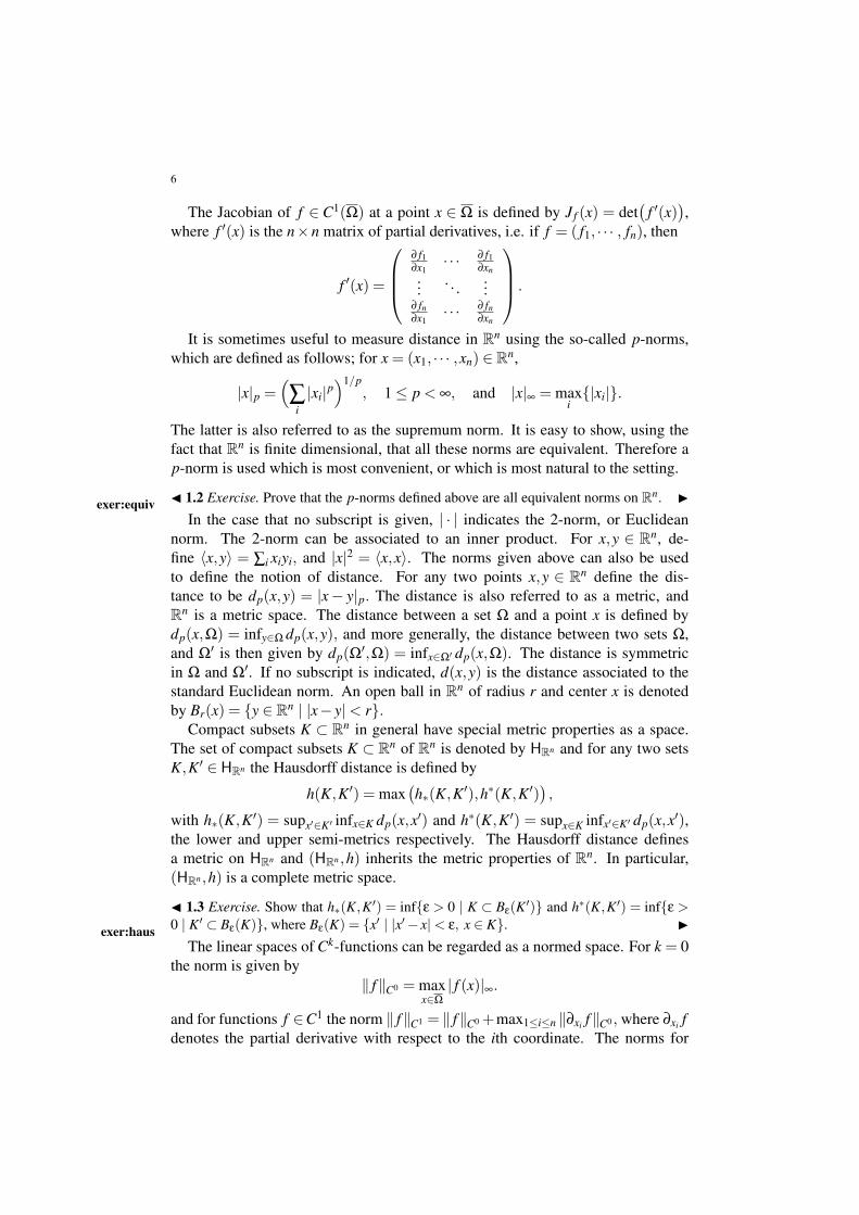
FIGURE 2.1. The pre-image of small neighborhood B&(p) is theunion of small neighborhoods N&(x j)"" diffeomorphic to B&(p).
! 2.2 Definition. For a regular value p -# f (#"), define the C1-mapping degreeby
deg( f ,", p) := $x# f!1(p)
sign)
Jf (x)*,
which takes values in Z. "defn:deg1
! 2.3 Exercise. Explain that when p # f (#") the degree is not stable under small pertur-bations. "exer:bound1! 2.4 Exercise. (Local continuity/stability of the degree in p) Show, that if p is regularwith p -# f (#"), there exists an & > 0 such that all p% # B&(p) are regular values for f . Usethis to prove that deg( f ,", p%) = deg( f ,", p) for all p% # B&(p) with & > 0 is small enoughso that p% -# f (#") for all p% # B&(p). "exer:bound2! 2.5 Exercise. (Local continuity of the degree in f ) Let p be a regular value for f withp -# f (#"). Show that there exists an & > 0 such that all for g #C1("), with + f !g+C1 <&, p is a regular value for g. Use this to prove that deg( f ,", p) = deg(g,", p) for all+ f !g+C1 < & with 0 < &' 1
2 d(p, f (#")) small enough so that p is a regular value for allsuch g. "exer:bound3fig:figc1deg1
Definition 2.2 of degree was used in the prelude to this chapter and gives aconvenient way of computing the mapping degree in the case of regular values p.The condition p -# f (#") is an isolation condition, and makes " a set that strictlycontains solutions of f (x) = p on ", i.e. " isolates the solution set f!1(p). Thisisolation requirement in the definition of degree equips the mapping degree withvarious robustness properties, see e.g. Exercise 2.3 - 2.5.
The definition yields a number of crucial properties. For the identity map f = Idthe degree is easily computed, i.e. if p #", then
(2.1) deg(Id,", p) = 1,
and for p -#", deg(Id,", p) = 0. Another important property that follows imme-eqn:e2diately from the definition is that the equations f (x) = p and f (x)! p = 0 have thesame solution set, and Jf = Jf!p. Therefore
(2.2) deg( f ,", p) = deg( f ! p,",0).
9
If "1,"2 "" are two disjoint, open subsets, such that p -# f!"\("1/"2)
", then eqn:e1
(2.3) deg( f ,", p) = deg( f ,"1, p)+deg( f ,"2, p)
eqn:e3
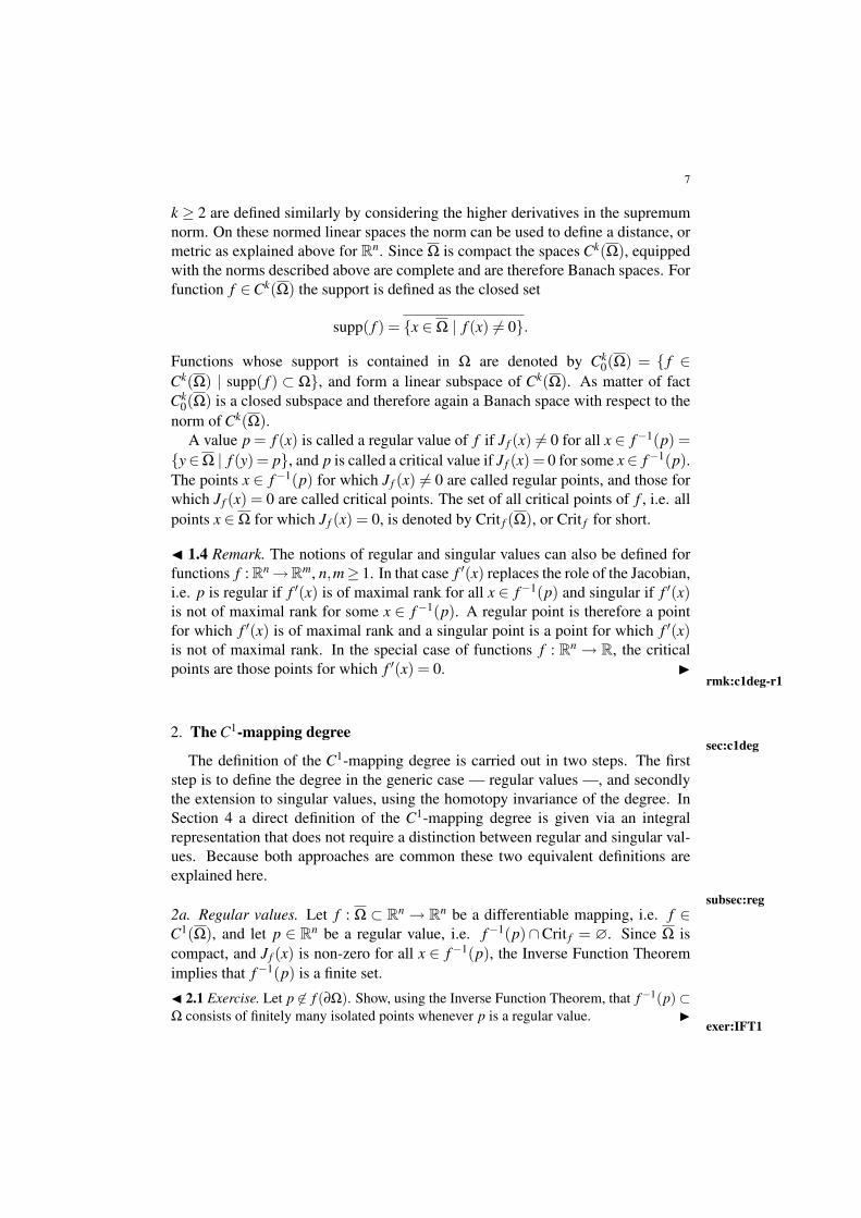
! 2.7 Example. Consider the mapping f : D2 " R2 $ R2 defined by f (x1,x2) =(2x2
1!1,2x1x2). This mapping gives a 2-fold covering of the disc. Figure 2.2 showsthat the boundary #D2 = S1 winds around the origin twice under the image of themap f . For the value (0,0), the pre-image consists of the points x1 = (!1
2
02,0)
and x2 = (12
02,0), and
f %(x1) =+!20
2 00 !
02
,, f %(x2) =
+20
2 00
02
,.
Therefore (0,0) is a regular value for f , and since Jf (x1) = Jf (x2) = +1, the degreeis given by deg( f ,D2,0) = 2. " ex:c1degex1
FIGURE 2.2. Winding S1 twice around the origin.
fig:figc1deg2
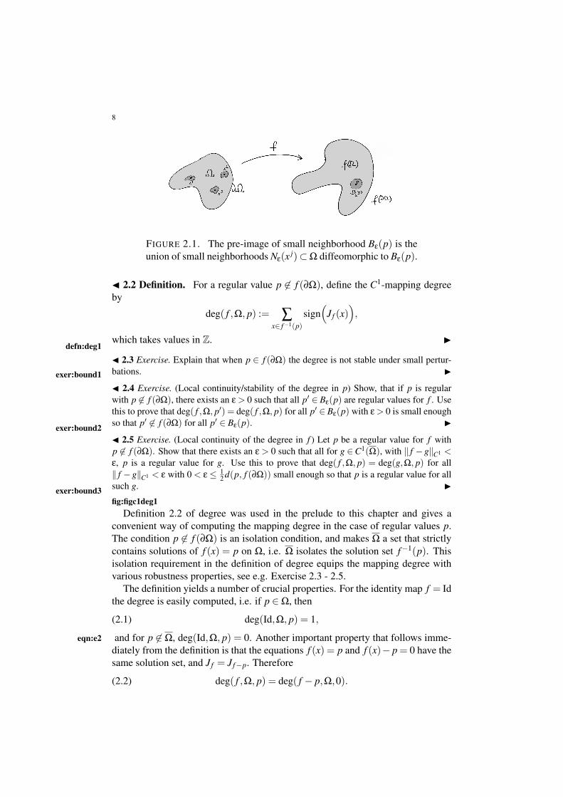
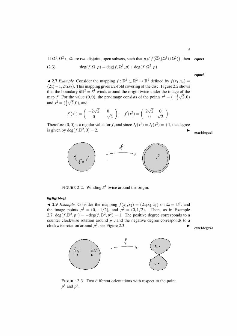
! 2.9 Example. Consider the mapping f (x1,x2) = (2x1x2,x1) on " = D2, andthe image points p1 = (0,!1/2), and p2 = (0,1/2). Then, as in Example2.7, deg( f ,D2, p1) = !deg( f ,D2, p2) = 1. The positive degree corresponds to acounter clockwise rotation around p1, and the negative degree corresponds to aclockwise rotation around p2, see Figure 2.3. " ex:c1degex2
FIGURE 2.3. Two different orientations with respect to the pointp1 and p2.

10
fig:figc1deg3Basically, for regular values p, the degree is a count of the elements in f!1(p)
with orientation, i.e. a point x j # f!1(p) is counted with either +1 or!1 wheneverf is locally orientation preserving or reversing respectively. The degree counts howmany times the image f (") covers p counted with multiplicity. This is a purelylocal but stable property for regular values, see also Section 5. Of course, whetherp is a regular value of a given function f or not is not always straightforward todecide. Sard’s Theorem (see Appendix 1b) claims that a value p is regular with‘probability’ 1. This fact can be used to extend the definition of degree to arbitraryvalues p (Chapter II).
! 2.11 Remark. A rougher version of degree is the so-called mod-2 degree and isdefined as follows; deg2( f ,", p) = #
)f!1(p)
*mod 2. This degree contains less
information than the degree defined in Definition (2.2), but will be of importancefor mappings between non-orientable spaces. See [12]. "
rmk:mod2
subsec:ht1 2b. Homotopy invariance. A crucial property of the C1-mapping degree is the ho-motopy invariance with respect to f . Large perturbations f which do not destroythe isolation along the homotopy leave the degree unchanged.
! 2.12 Lemma. Let t 1$ ft , t # [0,1] be a continuous path in C1("), with p -#ft(#") for all t # [0,1] and let p be a regular value for both f0 and f1. Thendeg( f0,", p) = deg( f1,", p). "
lem:pert1aProof: Let F(t, ·) = ft and consider the equation F(t,x) = p. By assumption
p is a regular value for both f0 and f1. From Theorem A.3 it follows that F canbe approximated arbitrarily close in C0 by a function -F #C%([0,1]&") such that-ft = F(t, ·) is arbitrary close to ft in C1, uniformly in t # [0,1]. By Sard’s Theorem(see Theorem A.5) we can choose value p% arbitrary close to p which is regular forboth F and -F . By the local stability of the degree (Exercise 2.4) there exists an & > 0such that deg( f0,", p%) = deg( f0,", p) and deg( f1,", p%) = deg( f1,", p) for allp% # B&(p). Using the local continuity of the degree, see Exercise 2.5, there existsa ' > 0 such that deg(-f0,", p%) = deg( f0,", p) and deg(-f1,", p%) = deg( f1,", p)for all p% # B&(p), and all maxt#[0,1] +-ft ! ft+C1 < '. For a regular value p% thesolution set -F!1(p%) of the equation
-F(t,x) = p%,
is a smooth 1-dimensional manifold with boundary given by #-F!1(p%) =. -f!10 (p%)& {0}
//
. -f!11 (p%)& {1}
/(see Appendix 1b). Since p -# ft(#") it holds
that p% -# -ft(#"), consequently -F!1(p%)" [0,1]&". Therefore, the 1-dimensionalcomponents diffeomorphic to [0,1] are curves connecting elements in #-F!1(p%)and components diffeomorphic to S1 are contained in (0,1)&", since p% is a reg-ular value for both -f0 and -f1. It’s worth mentioning that by the TransversalityTheorem (see Appendix 1b) p% is a regular value for -ft for almost every t # [0,1].
11
The manifold -F!1(p%) can be given a canonical orientation as follows. Since p% isregular the matrix
F %(t,x) =
#
$%#t -F1 #x1
-F1 · · · #xn-F1
......
. . ....
#t -Fn #x1-Fn · · · #xn
-Fn
&
'( ,
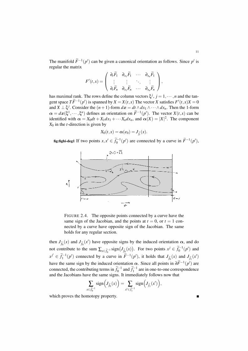
has maximal rank. The rows define the column vectors ( j, j = 1, · · · ,n and the tan-gent space T -F!1(p%) is spanned by X = X(t,x) The vector X satisfies F %(t,x)X = 0and X 2 ( j. Consider the (n+1)-form dx = dt 3dx13 · · ·3dxn. Then the 1-form! = dx((1, · · · ,(n) defines an orientation on -F!1(p%). The vector X(t,x) can beidentified with ! = X0dt + X1dx1 + · · ·Xndxn, and !(X) = |X |2. The componentX0 in the t-direction is given by
X0(t,x) = !(e0) = J-ft (x).
fig:fighi-deg1 If two points x,x% # -f!10 (p%) are connected by a curve in -F!1(p%),
FIGURE 2.4. The opposite points connected by a curve have thesame sign of the Jacobian, and the points at t = 0, or t = 1 con-nected by a curve have opposite sign of the Jacobian. The sameholds for any regular section.
then J-f0(x) and J-f0
(x%) have opposite signs by the induced orientation !, and donot contribute to the sum $x#-f!1
0sign
!J-f0
(x)". For two points x j # -f!1
0 (p%) and
x j% # -f!11 (p%) connected by a curve in -F!1(p%), it holds that J-f0
(x) and J-f1(x%)
have the same sign by the induced orientation !. Since all points in #-F!1(p%) areconnected, the contributing terms in -f!1
0 and -f!11 are in one-to-one correspondence
and the Jacobians have the same signs. It immediately follows now that
$x#-f!1
0
sign)
J-f0(x)
*= $
x%#-f!11
sign)
J-f1(x%)
*,
which proves the homotopy property.
12
! 2.14 Remark. If the assumption p -# ft(#"), for all t # [0,1], is removed the aboveproof may fail at a number of points. Most important to mention in this contextis that without the isolation property the points in #-F!1(p%) are not necessarilyconnected by a curve and the contributing terms in -f!1
0 and -f!11 are not necessarily
in one-to-one correspondence, see also Exercise 2.3. "rmk:is1Let D" Rn\ f (#") be any connected component,1 then the degree deg( f ,", p)
is independent of p # D. This easily follows from the homotopy principle.
! 2.15 Lemma. For any curve t 1$ pt #D, t # [0,1], with p0 and p1 regular values,it holds that deg( f ,", p0) = deg( f ,", p1). "
lem:hp1Proof: From Equation (2.2) it follows that deg( f ,", p0) = deg( f! p0,",0), and
deg( f ,", p1) = deg( f ! p0,",0). It holds that pt # D if and only if pt -# f (#").The homotopy ft = f ! pt therefore satisfies the requirements of Lemma 2.12, and
deg( f ,", p0) = deg( f ! p0,",0) = deg( f ! p0,",0) = deg( f ,", p1),
which proves the statement.
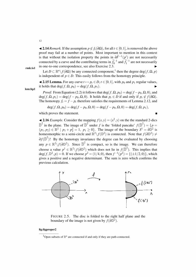
! 2.16 Example. Consider the mapping f (x,y) = (x2,y) on the the standard 2-dicsD2 in the plane. The image of D2 under f is the ‘folded pancake’ f (D2) = {p =(p1, p2) # R2 | p1 + p2
2 = 1, p1 , 0}. The image of the boundary S1 = #D2 ishomeomorphic to a semi-circle and R2\ f (D2) is connected. Note that f (#D2) -=# f (D2)! By the homotopy invariance the degree can be evaluated by choosingany p # R2\ f (#D2). Since D2 is compact, so is the image. We can thereforechoose a value p1 # R2\ f (#D2) which does not lie in f (D2). This implies thatdeg( f ,D2, p) = 0. If we choose p2 = (1/4,0), then f!1(p2) = {(±1/2,0)}, whichgives a positive and a negative determinant. The sum is zero which confirms theprevious calculation.
FIGURE 2.5. The disc is folded to the right half plane and theboundary of the image is not given by f (#D2).
fig:figproper2
1Open subsets of Rn are connected if and only if they are path-connected.

13
If we choose a path t 1$ pt connecting the regular values p1 and p2 and whichlies in R2\ f (#D2), then pt crosses the boundary # f (D2) in the vertical. However,pt -# f (#D2) for all t # [0,1] and the pre-image f!1(pt) # D2 for all t # [0,1]. Thevalues in f (D2) on the vertical are necessarily singular. This again shows that theboundary of the image should not be considered as a restriction on p. In the nextsubsection we show that the degree is defined for all p in R2\ f (#D2). "
ex:one-compThe previous example yields the following property of the mapping degree.
! 2.18 Lemma. Suppose that Rn\ f (#") is connected, then for any regular valuep # Rn\ f (#") is holds that deg( f ,", p) = 0. "
lem:one-comp1Proof: See Example 2.16.
subsec:arb12c. The degree for arbitrary values. The homotopy invariance established in theprevious subsection can be used now to extend the definition of the C1-mappingdegree to arbitrary values p # D, for any connected component of Rn\ f (#").
! 2.19 Definition. Let p # D, with D a connected component of Rn\ f (#"). Then
deg( f ,", p) := deg( f ,", p%),
for any regular value p% # D and thus deg( f ,", p) = deg( f ,",D). "defn:arbdeg1
By Sard’s Theorem (Appendix 1b, Theorem A.5) the regular values in D liedense in D. By Lemma 2.15 the choice of regular value p% does not matter andtherefore the extension of the degree as given by Definition 2.19 is well-defined.The properties of the generic degree listed in Equations (2.1) - (2.3) and Lemma2.12 also hold for the general C1-mapping degree and are the fundamental axiomsthat define a degree theory, see Section 7.
! 2.20 Theorem. The degree function deg( f ,", p) in Definition 2.19 satisfies thefollowing axioms:
(A1) if p #", then deg(Id,", p) = 1;(A2) for "1,"2 " ", disjoint open subsets of " and p -# f
!"\("1 /"2)
", it
holds that deg( f ,", p) = deg( f ,"1, p)+deg( f ,"2, p);(A3) for any continuous path t 1$ ft , ft #C1("), with p -# ft(#"), it holds that
deg( ft ,", p) is independent of t # [0,1];(A4) deg( f ,", p) = deg( f ! p,",0).
The application ( f ,", p) 1$ deg( f ,", p) is called a C1-degree theory. "thm:axioms1
Proof: Axiom (A1) follows immediately from Equation (2.1). As for Axiom(A2), by assumption, f!1(p)""1/"2 and therefore f!1(p%)""1/"2 for anyregular value p% sufficiently close to p. Consequently,
deg( f ,", p) = deg( f ,", p%) = deg( f ,"1, p%)+deg( f ,"2, p%)= deg( f ,"1, p)+deg( f ,"2, p).

14
Choose a value p% that is regular for both f0 and f1. If p% is chosen sufficientlyclose to p, then p% -# ft(#"), and thus by Lemma 2.12 and Definition 2.19
deg( f0,", p) = deg( f0,", p%) = deg( f1,", p%) = deg( f1,", p).
By considering the homotopy t 1$ ft0t it follows that deg( f0,", p) = deg( ft0 ,", p),for any t0 # [0,1], which proves Axiom (A3). Finally, let p% be a regular valuesufficiently close to p, then by Equation (2.3), deg( f ,", p) = deg( f ,", p%) =deg( f ! p%,",0). Consider the homotopy ft = (1! t)( f ! p) + t( f ! p%) =f ! (1! t)p! t p%. Since p% is close to p, the line-segment {(1! t)p + t p%}t#[0,1]does not intersect f (#"), and herefore 0 -# ft(#"). From Axiom (A3) it then fol-lows that
deg( f ,", p) = deg( f ,", p%) = deg( f ! p%,",0) = deg( f ! p,",0),
which proves Axiom (A4), and thereby completing the proof.
3. The general homotopy principlesec:c1deg-hi
The homotopy invariance established in the previous section allows for defor-mations in both f and p. Using the axioms of a degree theory one can prove thatthe domain " can also be varied. In Section 7 the homotopy principle will be de-rived from the axioms. In this section a direct proof using the definition will begiven.
subsec:var3a. Variations in domains. Let ! " Rn & [0,1] be bounded and relatively opensubset of Rn& [0,1]. Define the t-slices by
!t = {x | (x, t) #!}, t # [0,1]
and their boundaries by (#!)t = {x | (x, t) # #!} =!!
"t \!t .
Note that !t "!!
"t which is essential for the definition of (#!)t .
! 3.1 Definition. Two triples ( f ," f , p) and (g,"g,q) are said to be homotopic, orcobordant, if there exists a bounded and relatively open subset !"Rn& [0,1] anda continuous function F : !$ Rn, with ft = F(·, t) #C1(!t), such that
(i) f0 = f , and f1 = g;(ii) !0 = " f , and !1 = "g;
(iii) there exists a continuous path t 1$ pt , such that pt -# ft((#!)t) for all t #[0,1], and p0 = p and p1 = q.
Notation ( f ," f , p)4 (g,"g,q). Triples ( f ," f ,D f ) and (g,"g,Dg), for which theabove requirements are met, are also called homotopic. "
defn:hi-2

15
! 3.2 Theorem. Let ( f ," f , p) and (g,"g,q) be homotopic triples, then
deg( f ," f , p) = deg(g,"g,q).
In particular, deg( ft ,!t , pt) is constant in t # [0,1], where ft is a homotopy asdefined in Definition 3.1. "
thm:domain1Proof: From the definition of the degree we can choose values p% and q% which
are regular values of f and g respectively. The values p% and q% can be chosenarbitrary close to p and q. Then deg( f ," f , p) = deg( f ," f , p%) and deg(g,"g,q) =deg(g,"g,q%). Let p%t be a continuous path in ! connecting p% and q% and whichlies in an &-neighborhood of the path pt . Therefore, if & is chosen small enough,p%t -# ft((#!)t), for all t # [0,1]. By Axiom (A4) it holds that
deg( ft ,!t , p%t) = deg( ft ! p%t ,!t ,0),
for all t # [0,1]. Now consider the equation
G(t,x) = F(t,x)! p%t .
The proof now follows along the same lines as the proof of Lemma 2.12. The onlydifference is the domain !. By assumption, the solution set G!1(0) is contained in!, i.e. G!1(0). (#!)t = ! for all t # [0,1]. Choose a C%-perturbation -F , whichyields -G = -F! p%t . By Sard’s Theorem choose a regular value 0%, arbitrary close to0, and the solution set -G!1(0%) can be described in exactly the same way as in theproof of Lemma 2.12. Figure 3.1 below shows the slightly different situation withLemma 2.12. fig:fighi-deg2 The fact that deg( ft ,!t , pt) is constant in t in the same
FIGURE 3.1. Also in the case of general domains !" [0,1]&Rn
the the opposite points connected by a curve have the same sign ofthe Jacobian.
way as Axiom (A3).

16
! 3.4 Remark. For t # [0,1], let Dt be the connected component of Rn\ ft((#!)t)containing pt . Then the result of Theorem 3.2 can be reformulated as
(3.1) deg( ft ,!t ,Dt) = const.,
which establishes continuity of the degree in f , " and p. "eqn:c1deg-hirmk:hi-5
subsec:isol3b. The index of isolated zeroes. It the case that a mapping has only isolated ze-roes, and thus finitely many, Property (A3) gives the degree as a sum of the localdegrees. More precisely, let xi #" be the zeroes of f and let "i "" be sufficientlysmall small neighborhoods of xi #"i, such that xi the only solution of f (x) = p in"i for all i. Then deg( f ,", p) = $i deg( f ,"i, p) and we define
)( f ,xi, p) := deg( f ,"i, p),
which is called the index of an isolated zero of f . The index for isolated zero doesnot depend on the domain "i. Indeed, if "i and -"i are both neighborhoods of xi
for which xi is the only zero of f (x) = p, then we can define a cobordism between( f ,"i, p) and ( f , -"i, p) as follows. Let ! = /t#[0,1]!t with
!t =
012
13
"i for t < 12 ,
"i. -"i for t = 12 ,
-"i for t > 12 ,
and ft = F(·, t) = f , pt = p. By Theorem 3.2 deg( f ,"i, p) = deg( f , -"i, p). Theexpression for the degree becomes
(3.2) deg( f ,", p) = $x# f!1(p)
)( f ,x, p).
It is not hard to find mappings with isolated zeroes of arbitrary integer index.eqn:index2! 3.5 Exercise. Show that if x # f!1(p) is a non-degenerate zero of f , then )( f ,x, p) =(!1)*, where * = #{negative real eigenvalues} (counted with multiplicity). "exer:index3
4. The integral representation of the C1-mapping degreesec:intdegree
The expression for the C1-mapping degree for regular values points to a obviousintegral definition of the degree which allows for a formulation of of the C1-degreewithout distinguishing between regular and singular values. The integral formula-tion is is also useful sometimes for establishing various properties.
subsec:regint4a. Regular integrals. Let + : Rn $ R be a continuous function with supp(+) =B&(p). Choose & > 0 small enough such that supp(+) " Rn\ f (#") and is a coor-dinate neighborhood of p with respect to the change of coordinates p = f (x), seeFigure 2.1. The weight function can be normalized by
Z
Rn+(x)dx = 1.
A function + that satisfies the above conditions is called a weight function, or testfunction. In the calculations that follow it is convenient to use the notation of

17
differential forms on Rn. Write dx = dx13 · · ·3dxn as the standard n-form on Rn
and consider the differential n-forms
" = +(y)dy, and f *" = +( f (x))Jf (x)dx.
The latter is called the pullback under f , where y = f (x). The n-form dx providesRn with a standard orientation. With this notation a lot of the calculations sim-plify considerably. The space of compactly supported continuous n-forms on Rn isdenoted by ,n
c(Rn).
! 4.1 Lemma. Let p -# f (#") be a regular value and + a weight function as definedabove. Then the integral I represents the C1-mapping degree;
(4.1) I =Z
"f *" = deg( f ,", p).
" eqn:c1deg2lem:indep1Proof: As pointed out before f!1(p) is a finite set strictly contained in ". Since
Jf is non-zero at points in f!1(p) = {x1, ...,xk}, the Inverse Function Theoremgives that f maps neighborhoods N&(x j) of points in x j # f!1(p) diffeomorphicallyonto B&(p), see Figure 2.1. Thus f is a local change of coordinates near every pointin x j # f!1(p). Indeed, the fact that Jf is non-zero at points in x j # f!1(p), impliesthat Jf is also non-zero at the points in N&(x j), provided that & is small enough. Theintegral I splits in k local integrals
Z
"f *" = $
j
Z
N&(x j)f *" = $
jsign
)Jf (x j)
*Z
B&(p)"
= $j
sign)
Jf (x j)*
= deg( f ,", p),
which proves that both I is independent of + and represents the degree defined inDefinition 2.2. The above calculation uses that locally f is a coordinate transfor-mation y = f (x) and
R+( f (x))Jf (x)dx = sign
)Jf (xi)
*R+(y)dy.
! 4.2 Exercise. Verify the above change of coordinates formula given by y = f (x). " exer:ch1! 4.3 Remark. If in the above lemma we choose weight functions + with the prop-erty that
R" " -= 0, then
deg( f ,", p) ·Z
Rn" =
Z
"f *".
See also Remark 4.15. " rmk:weight1subsec:arb4b. A general representation. The integral characterization of the degree in the
generic case motivates a representation of the C1-degree in general, i.e. regard-less whether p is regular or not. In order for the integral representation in (4.1)to serve as a definition of degree for general p, the independence on + needs tobe established. As before let + be a continuous weight function on Rn with theproperties
supp(+)" D" Rn\ f (#"), andZ
Rn" = 1,
18
where D is the connected component of Rn\ f (#") containing p. The first prop-erty allows for a larger class of weight functions in the sense that supp(+) is notnecessarily a local coordinate neighborhood of p. The space of continuous n-forms " = +(x)dx, with supp(+) " D, are denoted by ,n
c(D). For " # ,nc(D)
andRRn " = 1 we define the integral over " by
(4.2) I( f ,",D) :=Z
"f *".
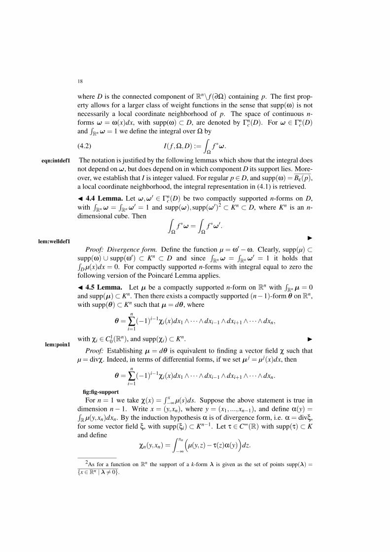
The notation is justified by the following lemmas which show that the integral doeseqn:intdef1not depend on ", but does depend on in which component D its support lies. More-over, we establish that I is integer valued. For regular p#D, and supp(+) = B&(p),a local coordinate neighborhood, the integral representation in (4.1) is retrieved.
! 4.4 Lemma. Let ","% # ,nc(D) be two compactly supported n-forms on D,
withRRn " =
RRn "% = 1 and supp("),supp("%)2 " Kn " D, where Kn is an n-
dimensional cube. Then Z
"f *" =
Z
"f *"%.
"lem:welldef1Proof: Divergence form. Define the function µ = +% !+. Clearly, supp(µ) "
supp(+) / supp(+%) " Kn " D and sinceRRn " =
RRn "% = 1 it holds thatR
D µ(x)dx = 0. For compactly supported n-forms with integral equal to zero thefollowing version of the Poincare Lemma applies.
! 4.5 Lemma. Let µ be a compactly supported n-form on Rn withRRn µ = 0
and supp(µ)" Kn. Then there exists a compactly supported (n!1)-form # on Rn,with supp(#)" Kn such that µ = d#, where
# =n
$i=1
(!1)i!1-i(x)dx13 · · ·3dxi!13dxi+13 · · ·3dxn,
with -i #C10(Rn), and supp(-i)" Kn. "
lem:poin1Proof: Establishing µ = d# is equivalent to finding a vector field - such that
µ = div-. Indeed, in terms of differential forms, if we set µ j = µ j(x)dx, then
# =n
$i=1
(!1)i!1-i(x)dx13 · · ·3dxi!13dxi+13 · · ·3dxn.
fig:fig-supportFor n = 1 we take -(x) =
R x!% µ(s)ds. Suppose the above statement is true in
dimension n! 1. Write x = (y,xn), where y = (x1, ...,xn!1), and define .(y) =RR µ(y,xn)dxn. By the induction hypothesis . is of divergence form, i.e. . = div(,
for some vector field (, with supp((i) " Kn!1. Let / # C%(R) with supp(/) " Kand define
-n(y,xn) =Z xn
!%
)µ(y,z)! /(z).(y)
*dz.
2As for a function on Rn the support of a k-form ! is given as the set of points supp(!) ={x # Rn | ! -= 0}.
19
FIGURE 4.1. The covering of supp(+)/ supp(+%) by Kn " D.
By Construction supp(-n)" Kn, and #-n#xn
= µ(x)! /(xn).(y). Now let
-(x) =!((y)/(xn),-n(y,xn)
",
then
div-(x) = /(xn)div((y)+#-n
#xn(x)
= /(xn).(y)+µ(x)! /(xn).(y)= µ(x),
and supp(-i)" Kn.
Now apply Lemma 4.5 to the form µ = "% !" with support in Kn " D. There-fore, µ = "% !" = d# for some compactly supported (n!1)-form #. Moreover,the support of the form # is contained in Kn " D.
Independence. The cube Kn"D has a piecewise smooth boundary and thereforeby Stokes’ Theorem
Z
"f *"% !
Z
"f *" =
Z
"f *("% !") =
Z
"f *µ
=Z
"f *d# =
Z
f!1(Kn)f *d#
=Z
f!1(Kn)d( f *#) =
Z
# f!1(Kn)f *# = 0,
since supp( f *#)" f!1(Kn)"". This proves the lemma.
! 4.7 Exercise. Check, using differential forms calculus, that f *d# = d( f *#) (Hint: showthis first for C2-functions). " exer:form2! 4.8 Remark. The first step of the proof of Lemma 4.4 holds for any two n-forms" and "% with compact support. This is essentially the Poincare Lemma as given byLemma 4.5. The second step is Stokes’ Theorem and uses in an essential way thatboth " and "% have their supports in D. If the latter does not hold then the integralsR
" f *" andR
" f *"% are not necessarily equal. As a consequence it will become

20
clear from the forthcoming discussion that p -# f (#") is an essential condition inorder for the integral definition of the degree to hold. "
rmk:c1degbd
! 4.9 Lemma. Let " # ,nc(D) with
RRn " = 1 and supp(")" Kn " D. Then
Z
"f *" = deg( f ,", p) # Z,
for any regular value p # supp("). "lem:intisZ
Proof: By Sard’s Theorem choose a regular value p # supp(") and choose acoordinate neighborhood B&(p)"Kn. As before choose "% with supp("%) = B&(p).From Lemma 4.1 it follows that
R" f *"% = deg( f ,", p) and from Lemma 4.4
Z
"f *" =
Z
"f *"% = deg( f ,", p),
which proves the lemma.
The next lemma shows that for any form " # ,nc(D), with support in some cube
Kn " D, the integrals are the same.
! 4.10 Lemma. Let ","% # ,nc(D) be two compactly supported n-forms on D,
withRRn " =
RRn "% = 1, and supp(")" Kn " D and supp("%)" K%n " D. Then
Z
"f *" =
Z
"f *"%,
and thereforeR
" f *" does not depend on p # D, but only on the connected com-ponent D. "
lem:diffsuppProof: Choose two balls B&(p) " supp(") and B&%(p%) " supp("%) and a curve
0 # D connecting p and p%. Cover 0 by finitely many small balls B& j(p j), j =1, · · · ,k, such that for any two conseccutive balls it holds that
B& j(p j)/B& j+1(p j+1)" Knj " D,
for some cube Knj . Let " j be forms with supp(" j) = B& j(p j). Then by Lemma 4.4
Z
"f *" j =
Z
"f *" j+1,
and thereforeZ
"f *" =
Z
"f *"1 = · · · =
Z
"f *"k =
Z
"f *"%,
which proves the lemma.
Lemma 4.10 justifies the notation I( f ,",D) and by Lemma 4.9 the integral isinteger valued. In particular, the above considerations prove that:
21
! 4.11 Lemma. For any regular values p, p% # D" Rn\ f (#") it holds that
deg( f ,", p) = deg( f ,", p%),
and I( f ,",D) = deg( f ,", p) for any regular value p # D. "lem:close1
It is is clear from the previous considerations that the degree is independent ofp#D and coincides with the definition of degree in the regular case; Definition 2.2.The advantage of the integral representation is that a lot of properties of the degreecan be obtained via fairly simple proofs. The final step is to show that one can useany compactly supported form " # ,n
c(D) to represent to the mapping degree.
! 4.12 Lemma. Let " # ,nc(D) with
RRn " = 1. Then
R" f *" = I( f ,",D). "
lem:anyomegaProof: Since supp(") " D is compact there exists a finite covering of open
balls U j = B& j(p j) with the additional property that U j " Knj " D for all j. Let
{1 j} be a partition of unity subordinate to {U j} and define the n-forms " j = 1 j"(see Appendix). It holds that $ j "
j = ", supp(" j) "U j. IfR
D " j -= 0, then byLemma 4.12 and Remark 4.3
(4.3) I( f ,",D) ·Z
D" j = deg( f ,", p j) ·
Z
D" j =
Z
"f *" j.
IfR
D " j = 0, then by Lemma 4.5, " j = d2 j and eqn:iddeg1Z
"f *" j =
Z
"f *d2 j =
Z
"d f *2 j = 0.
Therefore, Equation (4.3) holds for all j. Now sum over j in equation (4.3), whichthen proves the lemma.
This leads to the following alternative definition of the mapping degree for arbi-trary values p # D.
! 4.13 Definition. Let p # D" Rn\ f (#") and " # ,nc(D). Define
deg( f ,", p) := I( f ,",D) =Z
"f *",
as the C1-mapping degree. "defn:deg2
! 4.14 Exercise. Prove that deg( f ,", p) =R
" f *"/R
D " for any p # D " Rn\ f (#") andany " # ,n
c(D), withR
D " -= 0, i.e. " not exact. "exer:form3
! 4.15 Remark. The definition of the C1-mapping degree can formulated in termsof compactly supported cohomology; H*
c . Consider f : " $ Rn. By consideringa connected component D " Rn\ f (#") the map f yields a homomorphism f * incompactly supported cohomology via pull-back;
f * : Hkc!D)!$ Hk
c ("), ["] 1$ [ f *"],

22
where ["] is a non-trivial cohomology class in Hkc (D). Choose k = n, then follow-
ing diagram is a commutative diagram
Hnc (D) f *!!!!$ Hn
c (")
4=445
445R"
R deg( f ,",D)!!!!!!$ Rwhere the map
R" : Hn
c (")$ R is onto and the isomorphismR
D : Hnc (D)$ R is
given by ["]$R
D ". In the case that " is connected, thenR
" is an isomorphismbetween Hn
c (") and R. The commutativity of the diagram gives the relation
deg( f ,",D)Z
D" =
Z
"f *",
which is exactly the definition of the C1-mapping degree in Definition 4.13. "rmk:cohom
subsec:homtop2 4c. Homotopy invariance. The degree deg( f ,", p) is independent of p # D, withD " Rn\ f ("), a connected component. Therefore, for any curve t 1$ pt in D,deg( f ,", pt) is a constant function of t; the degree is invariant under homotopiesin p.
The integral representation of the degree can be used to establish homotopyinvariance of the degree with respect to f . In particular, since in the definition ofdegree the domain " isolates the solution set f!1(p), the degree is stable stableunder small perturbations of the map f , see Exercise 2.4. The general homotopyinvariance of the degree will be proved in several steps. The key ingredient is thecontinuity of the integral representation with respect to f .
! 4.16 Lemma. The function f 1$R
" f *" =R
" +( f (x))Jf (x)dx is continuous withrespect to the C1-topology. "
lem:hi-contProof: By the continuity of +(x), + f ! g+C1 < ', implies that |+( f (x))!
+(g(x))| < & uniformly for x # ". Similarly, since Jf (x) is a polynomial termin # fi
#x j, + f ! g+C1 < ' implies that |Jf (x)! Jg(x)| < &, uniformly in x # ". These
estimates combined yield the continuity of the integralR
" f *" with respect to f .
! 4.17 Lemma. Let t 1$ ft and t 1$ "t , t # [0,1] be a continuous paths in andassume that supp("t). ft(#") = ! for all t # [0,1], then
R" f *t "t = const. "
lem:pert0Proof: By assumption, for each t # [0,1] the integral represents a degree, i.e.R
" f *t "t = deg( ft ,", pt) for some pt # supp("). Therefore the integral is integervalued. On the other hand by Lemma 4.16 the integral is a continuous function oft and therefore constant.
We can use these lemmas to prove the general homotopy principle as given inTheorem 3.2.
23
! 4.18 Lemma. Let t 1$ ft and t 1$ pt , t # [0,1] be a continuous paths and assumethat pt -# ft(#") for all t # [0,1]. Then, deg( ft ,", pt) is a continuous function of tand is therefore constant along ( ft ,", pt). "
lem:pert1Proof: Choose an & > 0 small enough such that B&(pt) " Rn\ ft(#"). Define a
form " = +(x)dx such that supp(") = B&(0) and set "t = +(x! pt)dx. Conse-quently t 1$ "t is a continuous path with supp("t). ft(#") = ! for all t # [0,1]and
R" f *t "t = deg( ft ,", pt). By Lemma 4.17 the integral
R" f *t "t is constant,
which proves the lemma.
5. Proper mappingssec:proper
So far the mapping degree has been defined for mappings on bounded domains". For unbounded domains " the generic construction of the degree does not makesense in general due to the possible non-compactness of the set f!1(p). However,if a mapping is proper the C1-degree can be defined in the usual manner. Letf : "" Rn $ Rn be a proper mappings and " an unbounded domain. If p # Rn isa regular value then the degree deg( f ,", p) is given by Definition 2.2. The degreecan be extended to arbitrary values p following the procedures in Section 2c.
subsec:proper195a. Local and global degree. The integral representation in Section 4 can be usedthe define the C1-mapping degree for proper mappings for arbitrary values p di-rectly. Proper mappings are the natural morphisms that induce the homomorphismson compactly supported cohomology, see e.g. [4]. Using the construction in Sec-tion 4b yields to the following definition. Consider triples ( f ,", p), where ""Rn
is open, f : " " Rn $ Rn proper, and p -# Rn\ f (#"), and let " # ,nc(D), withR
D " = 1, where D" Rn\ f (#") a connected component containing p. Then
deg( f ,", p) :=Z
"f *".
As before the degree is independent of p # D and is therefore sometimes writtenas deg( f ,",D). If p is a regular value then the degree is given by Definition 2.2.In particular, for proper mappings from Rn to Rn the degree does not depend onp and is defined as deg( f ). The identity map on Rn is an example of a propermap, and deg(Id) = 1. The theory discussed in the remainder this chapter willmainly concern bounded sets ". However, if f : ""Rn $Rn is a proper mappingthe degree deg( f ,", p) can be computed by choosing a bounded domain "% "" containing f!1(p). In that case deg( f ,", p) = deg( f ,"%, p), which is usefulfor translating various properties of the degree for proper mappings. The degree( f ,", p) 1$ deg( f ,", p) is a local degree, or degree over p (cf. [7], IV, §5). Aspointed out before, for a regular value p the local degree counts the number timesthe set f!1(p) covers p (counted with multiplicity) under the mapping f , see Figure5.1. The degree depends on p (per connected component of Rn\ f (#")).

24
! 5.1 Example. Consider the function f : [!3,3]"R$R given by f (x) = x3!3x.The value p = 1 is regular and deg( f , [!3,3],1) = 1. The Figure 5.1 below showshow the image f ([!3,3]) covers p = 1. If we consider p = !20 (see Figure 5.1)then p is not covered by by the image under f and the degree is zero. "
proper0
FIGURE 5.1. The image f ([!3,3]) locally covers the regularvalue p = 1 and no covering at p =!20.
fig:figproper1In the case " = Rn and f : Rn $ Rn is proper, then the mapping degree
deg( f ,Rn, p) is independent of p and is denoted by deg( f ). In this case we re-fer to the global mapping degree (cf. [7], IV, §4). The global mapping degreecounts how many times f (Rn) covers Rn counted with multiplicity. The notion oflocal and global degree will be discussed in more depth in Section 10.
! 5.3 Example. Consider the polynomial function f (x) = x4!2x2 + 1 defined onR is a proper mapping. Choose a weight function
+(x) =
6(1! |x|) when x # [!1,1],0 otherwise.
Via the integral definition the degree is given by
deg( f ) =Z
Rf *" =
Z 02
0
.1! |x4!2x2 +1|
/.4x3!4x
/dx = 0,
which also follows from counting f!1(p) for any regular value p. "ex:proper2
! 5.4 Example. The polynomial function f (x) = x3! x/2 defined on R is also aproper mapping. Let 2+(2x) be a weight function, + as above, then
deg( f ) =Z
Rf *" =
Z 1
!1
.1!2|x3! x|
/.3x2!1/2
/dx = 1,
which proves that f (x) = p has at least one zero for any p # R. Functions + withfinite mass and which decrease monotonically to zero as |x| $ %, can be used

25
to approximate weight functions. For example take + = e!x2 and consider themapping f (x) = x3. Then
RR +(x) =
RR e!x2 =
03, and
deg( f ) =103
Z
Rf *" =
303
Z
Rx2e!x6
dx = 1,
which is of course the same answer as before. "ex:proper2
The examples suggest that for proper mappings from Rn to Rn the degree isrelated to surjectivity.
! 5.5 Lemma. Let f : Rn $ Rn be a proper C1-mapping.
(i) If deg( f ) -= 0, then f is surjective.(ii) If f is not surjective, then deg( f ) = 0.
When f is surjective deg( f ) counts (with multiplicity) how many times the imageunder f covers Rn. "
lem:surj1Proof: If deg( f ) -= 0, then the equation f (x) = p has a solution for any p # Rn
and thus f is surjective, proving (i).On the other, if f is not surjective then there exists a p and & > 0 such that
f (Rn).B&(p) = !, since proper mappings are closed mappings. Now choose ",with supp(")" B&(p). Then deg( f ) =
RR f *" = 0, which proves (ii) and therefore
the lemma.
! 5.6 Exercise. Give an example of an improper function f : R$R such that f!1(p) -= !for all p # R. "
exer:imp1
! 5.7 Exercise. Show that the formula deg( f ) = 13n/2
RRn e!| f (x)!p|2 Jf (x)dx, p # Rn, is an
alternative expression for the mapping degree for proper mappings f on Rn. "exer:alt1
! 5.8 Remark. In terms of compactly supported De Rham cohomology (Remark4.15) the local degree is again expressed via [ f *"] # Hn
c (") with ["] # Hnc (D),
p # D a connected component of Rn\ f (#"). Properness is needed to ensure thatf *" deteremines a cohomology class in Hn
c ("). In the case of the global degree[ f *"] = deg( f )["]. The compactly supported De Rham cohomology is homotopyinvariant with respect to proper homotopies (cf. [13], §44, [4], I, §2) and deg( f ) isa homotopy invariant. "
rmk:proper10
subsec:proper205b. Proper mappings on open subsets. We can restate the degree theory developedin this chapter for smooth mappings between open subsets of Rn. Let N,M " Rn
be open subsets. Note that we do not assume boundedness, nor connectedness ofN and M. Let f : N $ M be a mapping of class C1; f #C1(N;M). We start withremarking that when f!1(p) is compact then deg( f ,N, p) is defined.

26
! 5.9 Exercise. Give an example of a function f : R$R for which f!1(0) is compact andfor which f!1(p) is unbounded for any p -= 0 close to 0. " ex:proper21a
Let B&!
f!1(p)"" M, then the compactness of #B& yields that p -# f (#B&).
Define the local degree over p by deg( f ,N, p) := deg( f ,B&, p). This definitionholds for any compact neighborhood (open interior is needed) K& " N that con-tains f!1(p) in its interior and is independent of K& by Theorem 3.2 (comparethe arguments for the index of an isolated zero in Section 3b). This shows thatdeg( f ,N, p) is well-defined. We now give a general definition of local degree overcompact sets K "M (cf. [7], IV, §5 and VIII, §4, where the local degree is definedfor any continuous mapping, see also Section 10).
! 5.10 Definition. Let K "M ( -= !) be compact, connected and f!1(K) is com-pact. Then the local degree over K is defined by deg( f ,N,K) := deg( f ,N, p) forany p # K. "
defn:proper21
! 5.11 Lemma. The local degree deg( f ,N,K) is well-defined. "lem:proper24
Proof: Let K% " N be a compact neighborhood that contains f!1(K) is its inte-rior and consider the (restriction) mapping f : K% "N $M. By the compactness off (#K%) and K it follows that d( f (#K%),K), ' > 0 and thus K. f (#K%) = !. SinceK is connected it lies in a connected component D of M\ f (#K%). From Lemma2.18 and Definition 2.19 it follows that deg( f ,K%,D) only depends on D. Since forp # K " D it holds that deg( f ,N, p) = deg( f ,K%, p) we showed that deg( f ,N, p)is the same for every p # K.
! 5.12 Exercise. Show that d( f (#K%),K), ' > 0 in the proof of Lemma 5.11. "ex:proper23For any two connected sets K% " K " M it holds that deg( f ,N,K%) =
deg( f ,N,K). This definition is reminiscent of the degree as presented in Defi-nition 2.19. The above considerations reveal that the local degree deg( f ,N,K) canalso be characterized in terms of the integral representation. Let D"M\ f (#K%) bethe connected component containing K and " # ,n
c(D) such thatR
M " = 1, thendeg( f ,N,K) =
RK% f *".
A mapping f : N $ M is said to be proper over M% " M if f!1(K) is com-pact for all compact subsets K " M%. The degree deg( f ,N,K) is well-definedfor all compact sets K " M%. If M% is open and connected then the local degreedeg( f ,N, p) = deg( f ,N, p%) for any p, p% #M% (connect p and p% by a path 0 whichis a compact set). In this case we have the degree deg( f ,N,M%). From the latterthe degree for bounded domains follows as a special case.! 5.13 Example. Let " be a bounded domain and let f : " " Rn $ Rn be a C1-mapping, then f : "$Rn is a smooth mapping with N = " and M = Rn. Let D"Rn\ f (#") be a connected component, then for any compact subset K "D it holdsthat f!1(K) is closed and contained in " which implies that f!1(K) is compact.Therefore f # C1(";Rn) is proper over D and the local degree deg( f ,",D) iswell-defined. "ex:proper25
27
! 5.14 Definition. Let f : N $M be a proper C1-mapping and let M be connected.Then the global degree is defined by deg( f ) = deg( f ,N,K) for any compact subsetK with K "M (not necessarily connected). "
defn:proper22The global degree is well-defined since deg( f ,N,K) is independent of K
(connected) and by the above arguments deg( f ,N,K1 /K2) = deg( f ,N,K1) =deg( f ,N,K2) (connect by a path). The degree deg( f ) counts how many timesf (N) covers M counted with multiplicity, i.e. each sheet is either positively ornegatively oriented.
! 5.15 Example. Let ","% "Rn be bounded domains and f : ""Rn$"% "Rn bea C1-mapping. Suppose now that f : "$"% with N = " and M = "%, and f (#")"#"%. For any compact set K " "% it holds that f!1(K) " " and is compact. Themapping f #C1(","%) is proper and the degree deg( f ) = deg( f ,",K) is a globaldegree. If we only assume that f (#")" #"%, then f : "\ f!1(#"%)$"%. Also inthis case f is proper and deg( f ) is the global mapping degree. " ex:proper26
The homotopy of the global degree is exactly as explained before is we con-sider proper homotopies. For the local degree one needs to consider homo-topies ft for which f!1
t (K) is compact along the homotopy. Other propertiesstay more or less the same and we will come back to this in a more generalsetting in Section 10. For mappings that a proper over an open set M% " M thedegree can also be expressed via the integral representation. Let " # ,n
c(M%)with
RM% " = 1, then deg( f ,N,M%) =
RN f *". For the global degree (M% = M)
this gives deg( f ) =R
N f *". In Example 5.15 the degree is of course given bydeg( f ) =
R" f *" where " # ,n
c("%) andR
"% " = 1.! 5.16 Remark. In the case that " and "% are bounded domains with smooth bound-ary and f (#"%) " #"% we have the following commuting diagram. By the lattercondition f is a mappings of pairs, i.e. f : (",#")$ ("%
,#") and
Hnc (")
4=5!!!! Hn(",#") f *5!!!! Hn("%,#"%)
4=5!!!! Hnc ("%)
4=445
4454=
Hn!1(#")4*5!!!! Hn!1(#"%)
where 4 = f |#". From this diagram it follows that [ f *"] = deg( f )["] and[4*#] = deg(4)[#] and thus deg( f ) = deg(4). In Section 8 we will come backto the boundary dependence of the degree. In Section 10 we will give a moredetailed account of the algebraic topology. " rmk:proper27
NotesThe C1-mapping degree as considered in this first chapter was introduced by
Nagumo in 1951 [15]. In his paper Nagumo diverts from the definition of the map-ping the for continuous mappings by approximation via simplicial mappings, byapproximation via smooth mappings and defines the mapping degree for smoothmappings as was given in Definition 2.2. The mappings degree for continuous

28
functions, or Brouwer degree was developed by Brouwer [5] and is treated in Chap-ter II, where we follow the approach of Nagumo. In a series of papers Nagumoalso treats the degree in a more general settings such as the Leray-Schauder de-gree [14, 15, 16], see Chapter V. The generic definition of the C1-mapping degreeis useful often for computing the degree in specific situations. This definition ofthe mapping degree ties in with the homotopy argument in Lemma 2.12 and canfound for example in [12] and [16]. The homotopy principle can be applied inmany situations, see Chapter IV. The properties proved in Theorem 2.20 are ax-ioms for a degree theory and can be used in a much broader context, see ChapterII. In [1] Amman & Weiss show that the properties, or axioms uniquely determinethe degree. Heinz [9] gave an integral formulation of the smooth mapping degree.In Section 4 we essentially followed the treatments in [17] and [18]. The integralrepresentation in Section 4 provides a definition of the degree for smooth functionswithout having to worry about regular versus non-regular values. This definitionis based on the definition using compactly supported De Rham cohomology. Thedefinition of degree extends to mappings between smooth manifolds and to map-pings on unbounded domains — proper mappings, see Chapter II. In Chapter IIa direct definition of the degree for continuous functions is linked to a homologi-cal definition of the degree. Further elementary accounts of the degree for smoothfunctions in the context of bounded domains can be found in many books on non-linear analysis. We mention in particular the books by Berger [3], Nirenberg [17]and Schwartz [16]. See also Guillemin & Pollack [8], Malchiodi & Ambrosetti [2],Brown [6], Lloyd [11], Bott & Tu [4].
Exercises1: By identifying C and R2 the application z 1$ zn can be identified with a
smooth mapping f on R2. Show that )( f ,0) = n. Find a class of mappingson R2 for 0 is an isolated zero and )( f ,0) =!n.
2: Let f #C1("), with ""Rn a bounded domain and f is one-to-one. Provethat deg( f ,", p) = ±1.
3: Let f : B1(0)$ Rn and f (x) -= µx for µ, 0 and for all x # #B1(0). Showthat f (x) = 0 has a non-trivial solution in B1(0).
4: Let f (x) = anxn +an!1xn!1 + · · ·+a1x+a0 be a polynomial with an -= 0.(i) Show that for fixed coefficients a0, · · · ,an there exists an r > 0 such
that f!1(0) # (!r,r).(ii) Prove for n odd that deg( f ,(!r,r),0) = 1.
(iii) Prove that n even that deg( f ,(!r,r),0) = 0.(Hint: use the integral representation of the degree with +(x) = 1! x2 on(!1,1) and zero outside).
5: Prove Lemma 2.18.6*: (Borsuk’s Theorem) Let " " Rn be a bounded domain satisfying the
property that x #" implies that !x #". Let 5 : #""Rn $ Rn\{0} suchthat 5(!x) = !5(x). Prove that for any continuous extension f : " "Rn $ Rn of 5 it holds that deg( f ,",0) is an odd integer.

29
II. The Brouwer degree and theaxioms of degree theory
ch:BR2The C1-mapping degree defined in Chapter I strongly uses the fact that f is
differentiable. The homotopy invariance of the C1-degree can be used to extendthe degree to the class of continuous functions on Rn, which is essentially theapproach due to Nagumo [15]. At the core of the definition of the C0-mappingdegree, or Brouwer degree is the fact that C1-functions can be approximated byC0-functions. We will discuss the Brouwer for bounded and unbouded domains, aswell as for functions between manifolds. Another aspect is the axiomatic approachtowards degree theory. This will discussed for the Brouwer degree. At the end ofthis chapter we will also discuss the homological definition of the degree whichallows a direct definition of the Brouwer degree.
6. The Brouwer degreesec:c0approx
Using approximation of f via smooth mappings and homotopy invariance leadsto the definition of the C0-degree, or Brouwer degree
! 6.1 Definition. Let f #C0(") and let p -# f (#"). Then, for any sequence f k #C1(") converging to f in C0, define
deg( f ,", p) := limk$%
deg( f k,", p),
as the Brouwer degree of the pair ( f ,", p). "defn:c0degree
The properties of the C1-mapping degree imply that this definition makes sense,i.e. the limit exists and is independent of the chosen sequence f k. First of allapproximating sequences exist by virtue of Theorem A.3. Second, since p #Rn\ f (#") it holds that ' = d(p, f (#")) > 0 (compactness of "). Let g, g #C1(")be approximations of f such that +g! f+C0 ,+g! f+C0 < '/2. Consider the homo-topy ht(x) = (1! t)g(x)+ tg(x), t # [0,1]. fig:figc0deg1a The choices of g and ggive
+ht ! f+C0 ' (1! t)+g! f+C0 + t+g! f+C0
< (1! t) '/2+ t '/2 = '/2,
and for x # #" it holds that
|ht ! p|, | f ! p|!|ht ! f |, '/2.
Therefore, p -# ht(#") for all t # [0,1] and the degree deg(ht ,", p) is constantin t by the homotopy invariance of the degree (e.g. Lemma 4.18). We concludethat deg(g,", p) = deg(g,", p). For any approximating sequence f k it holds that
30
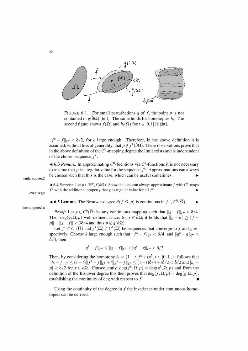
FIGURE 6.1. For small perturbations g of f , the point p is notcontained in g(#") [left]. The same holds for homotopies ht . Thesecond figure shows f (") and ht(") for t # [0,1] [right].
+ f k ! f+C0 < '/2, for k large enough. Therefore, in the above definition it isassumed, without loss of generality, that p -# f k(#"). These observations prove thatin the above definition of the C0-mapping degree the limit exists and is independentof the chosen sequence f k.
! 6.3 Remark. In approximating C0-fucntions via C1-functions it is not necessaryto assume that p is a regular value for the sequence f k. Approximations can alwaysbe chosen such that this is the case, which can be useful sometimes. "
rmk:approx2
! 6.4 Exercise. Let p#Rn\ f (#"). Show that one can always approximate f with C1-mapsf k with the additional property that p is regular value for all f k. "
exer:regu
! 6.5 Lemma. The Brouwer degree d( f ,", p) is continuous in f #C0("). "lem:approx1a
Proof: Let g # C0(") be any continuous mapping such that +g! f+C0 < '/4.Then deg(g,", p) well-defined, since, for x # #", it holds that +g! p+ , + f !p+!+g! f+ , 3'/4 and thus p -# g(#").
Let f k #C1(") and gk(") #C1(") be sequences that converge to f and g re-spectively. Choose k large enough such that + f k! f+C0 < '/4, and +gk! g+C0 <'/4, then
+gk! f+C0 ' +g! f+C0 ++gk!g+C0 < '/2.
Then, by considering the homotopy ht = (1! t) f k + tgk, t # [0,1], it follows that+ht ! f+C0 ' (1! t)+ f k! f+C0 + t+gk! f+C0 ' (1! t)'/4+ t'/2 < '/2 and |ht !p| , '/2 for x # #". Consequently, deg( f k,", p) = deg(gk,", p) and from thedefinition of the Brouwer degree this then proves that deg( f ,", p) = deg(g,", p),establishing the continuity of deg with respect to f .
Using the continuity of the degree in f the invariance under continuous homo-topies can be derived.

31
! 6.6 Lemma. For any continuous path t 1$ ft in C0("), with f0 = f and p -#ft(#"), t # [0,1], it holds that deg( ft ,", p) = deg( f ,", p) for all t # [0,1]. "
lem:approx1bProof: By definition t 1$ ft is continuous in C0(") and therefore by Lemma 6.5,
deg( ft ,", p) depends continuously on t # [0,1]. Since the degree is integer valuedit has to be constant along the homotopy ft .
! 6.7 Lemma. The Brouwer degree satisfies the translation property, i.e. for anyq # Rn it holds that d( f !q,", p!q) = f ( f ,", p). "
lem:approx5Proof: Choose a sufficiently small perturbation g # C1(") of f , then Axiom
(A4) implies that
deg(g!q,", p!q) = deg(g!q! (p!q),",0)= deg(g! p,",0) = deg(g,", p).
By definition deg( f ! q,", p ! q) = deg(g ! q,", p ! q) and deg( f ,", p) =deg(g,", p), which proves the lemma.
! 6.8 Remark. If t 1$ pt is a continuous path such that pt -# ft(#"), then the trans-lation property of the degree, Lemma 6.7, shows, since ft ! pt is a homotopy, that
deg( ft ,", pt) = deg( ft ! pt ,",0) = deg( f ! p,",0) = deg( f ,", p).
Therefore, the Brouwer degree is an invariant for cobordant triples ( f ,", p) 4(g,",q), or ( f ,",D) 4 (g,",D%). In the Section 7 the more general version willbe given allowing variations in ". "
rmk:approx6
7. Properties and axioms for the Brouwer degreesec:props1
In this section a number of useful properties of the mapping degree will begiven. In principle these properties can be proved using the definitions of the C1-mapping degree and the Brouwer degree. Another approach is to single out themost fundamental properties and show that these determine the Brouwer degreeuniquely, and that all properties can be derived from the axioms. Consider triples( f ,", p), where ""Rn are open sets, f #C("), and Rn 6 p -# f (#"). Such tripleare called admissible, and the mapping ( f ,", p) $ deg( f ,", p), which satisfiesthe following three axioms;
(A1) if p #", then deg(Id,", p) = 1;(A2) for "1,"2 " ", disjoint open subsets of ", and p -# f
!"\("1 /"2)
", it
holds that deg( f ,", p) = deg( f ,"1, p)+deg( f ,"2, p);(A3) for any continuous paths t 1$ ft , ft #C0(") and t 1$ pt , with pt -# ft(#"),
i.e. ( ft ,", pt) is admissible for all t, it holds that deg( ft ,", pt) is indepen-dent of t # [0,1];
is called a degree theory.

32
! 7.1 Theorem. The Brouwer degree deg( f ,", p) for admissible triples ( f ,", p)satisfies the Axioms (A1)-(A3), i.e. the Brouwer degree is a degree theory. "
thm:Brouwer1Proof: In order to verify Axiom (A1) consider the equation x = p. Clearly, there
exists a unique solution and JId(x) = Id, which proves (A1). Axiom (A3) followsfrom Lemma 6.6 and Remark 6.8.
Let 6 = "\("1 /"2), which is a closed subset in ", and "\6 = "1 /"2.Therefore, f
!"\("1/"2)
"= f (#")/ f (6), and since p -# f (6), it follows that
deg( f ,"\6, p) = deg( f ,"\6,D\ f (6)) =Z
"\6f *".
Because, supp(")" D\ f (6) and f (6). (D\ f (6)) = !, it holds thatZ
"\6f *" =
Z
"f *",
thereby proving that deg( f ,"\6, p) = deg( f ,", p). Now
deg( f ,", p) = deg( f ,"1/"2, p)= deg( f ,"1, p)+deg( f ,"2, p).
The latter is proved as follows:
deg( f ,"1/"2, p) = $i
Z
"i
f *" = $i
deg( f ,"i, p),
which proves the additivity property of the Brouwer degree.
! 7.2 Remark. For the Brouwer degree for maps from Rn to Rn, Axiom (A3) isequivalent to the following two alternative axioms:
(A3%) for any continuous path t 1$ ft , ft # C0(") and p -# ft(#"), it holds thatdeg( ft ,", p) is independent of t # [0,1];
(A4) deg( f ,", p) = deg( f ! p,",0).If the degree is considered for mappings between manifolds Axiom (A4) need notbe well-defined. "rmk:Brouwer2! 7.3 Exercise. Show that the (A3%) and (A4) combined are equivalent to (A3). "exer:ax-eq
The above theorem shows that there exists a degree theory satisfying Axioms(A1)-(A3); the Brouwer degree. The remainder of this section is a list of propertiesthat are derived from Axioms (A1)-(A3) and a proof that the Brouwer degree is theonly degree satisfying (A1)-(A3).
! 7.4 Property. (Validity of the degree) If p -# f ("), then deg( f ,", p) = 0. Con-versely, if deg( f ,", p) -= 0, then there exists a x #", such that f (x) = p. "pt:prop1
Proof: By chosing "1 = " and "2 = ! it follows from Axiom (A2) thatdeg( f ,!, p) = 0. Now take "1 = "2 = ! in Axiom (A2), then deg( f ,", p) =2 ·deg( f ,!, p) = 0.
Suppose that there exists no x # ", such that f (x) = p, i.e. f!1(p) = !. Sincep -# f (#"), it follows that p -# f ("), and thus deg( f ,", p) = 0, a contradiction.

33
! 7.5 Property. (Continuity of the degree) The degree deg( f ,", p) is continuousin f , i.e. there exists a ' = '(p, f ) > 0, such that for all g satisfying + f !g+C0 < ',it holds that p -# g(#"), and deg(g,", p) = deg( f ,", p). " pt:prop2
Proof: See Lemma 6.5.
! 7.6 Property. (Dependence on path components) The degree only depends onthe path components D"Rn\ f (#"), i.e. for any two points p,q #D"Rn\ f (#")it holds that deg( f ,", p) = deg( f ,",q). For any path component D " Rn\ f (#")this justifies the notation deg( f ,",D). " pt:prop4
Proof: Let p and q be connected by a path t 1$ pt in D, then by Axiom (A3),with ft = f , the degree deg( f ,", pt) is constant in t # [0,1].
! 7.7 Property. (Translation invariance) The degree is invariant under translation,i.e. for any q # Rn it holds that deg( f !q,", p!q) = deg( f ,", p). " pt:prop5
Proof: The degree d( f ! tq,", p! tq) is well-defined for all t # [0,1]. Indeed,since p!tq -# f (#")!tq, it follows from Axiom (A3) that deg( f !tq,", p!tq) =deg( f ,", p), for all t # [0,1].
! 7.8 Property. (Excision) Let 6"" be a closed subset in ", and p -# f (6). Then,deg( f ,", p) = deg( f ,"\6, p). " pt:prop6
Proof: In Axiom (A2) set "1 = "\6 and "2 = !, then deg( f ,", p) =deg( f ,"\6, p)+deg( f ,!, p) = deg( f ,"\6, p).
! 7.9 Property. (Additivity) Suppose that "i " ", i = 1, · · · ,k, are disjoint opensubsets of ", and p -# f
!"\(/i"i)
", then deg( f ,", p) = $i deg( f ,"i, p). "
pt:prop7Proof: The property holds trivially for k = 1. Now assume it holds for k! 1,
then by Axiom (A2)
deg( f ,", p) = deg)
f ,k!1[
i=1"i, p
*+deg( f ,"k, p) =
k
$i=1
deg( f ,"i, p),
by the induction hypothesis.
! 7.10 Exercise. Show that the above statement holds true for countable collections ofdisjoint open subsets "i of ". " exer:prop1-1
Let !" Rn& [0,1] be a bounded and relatively open subset of Rn& [0,1] (Sec-tion 3a), and let F : !$ Rn a continuous function on !, with ft = F(·, t), suchthat
(i) f0 = f , and f1 = g;(ii) !0 = " f , and !1 = "g;
(iii) there exists a continuous path t 1$ pt , p0 = p and p1 = q, such that ( ft ,!t , pt)is admissible for all t # [0,1];
then ( f ," f , p) 4 (g,"g,q) are homotopic, or corbordant (notation: ( f ," f , p) 4(g,"g,q)), and ( ft ,!t , pt) is an admissible homotopy. Compare this with Defini-tion 3.1 for the smooth mapping degree.
34
! 7.11 Property. (Homotopy invariance) For an admissible homotopy ( ft ,!t , pt),the degree deg( ft ,!t , pt) is constant in t # [0,1]. "
pt:prop3Proof: Following the proof Theorem 3.2 assume with loss of generality that
pt = p for all t. Choose a small ball B&(p), then following the reasoning in theproof of Theorem 3.2, f!1
t (B&(p))"Cti , t # (ti!'i, ti +'i), for finitely many setsCti "!. By excision, Property 7.8, it follows that deg( ft ,!t , p) = deg( ft ,Cti , p),and since the sets Cti&(ti!'i, ti +'i) form an open covering of F!1!B&(p)& [0,1]
",
the degree deg( ft ,!t , p) is constant for all t # [0,1].By (A4) deg( ft ,!t , pt) = deg( ft ! pt ,!t ,0). Therefore, without loss of gener-
ality, assume that pt = p is constant.Choose & > 0 small enough such that B&(p) " Rn\/t#[0,1] f ((#!)t). As be-
fore, write deg( ft ,!t , p) =R!t
f *t " =R(!)t
f *t ", where supp(") = B&(p). Byassumption, the set F!1!B&(p)& [0,1]
"# ! is compact. At every t # [0,1], the
sets f!1t (B&(p)) can be covered by open cylinders Ct & (t ! ', t + ') " !. At
each t, by compactness and continuity of F , ' can be small enough such thatf!1t % (B&(p)) " Ct % & (t % ! ', t %+ ') for all t % # (t! ', t + '). For all t # [0,1] these
sets form an open covering of F!1!B&(p)& [0,1]", which has a finite subcover-
ing, Cti & (ti ! 'i, ti + 'i), i = 1, · · · ,k. Therefore, for given t % # (ti ! 'i, ti + 'i),R!t
f *t %" =R
f!1t% (B&(p)) f *t %" =
RCti
f *t %", which is continuous in t % by Lemma 4.16 andthus constant in t %. Since the sets Cti & (ti! 'i, ti + 'i), i = 1, · · · ,k, form an opencovering, the degree is the same for all t # [0,1].
! 7.12 Property. (Orientation) Let A # GL(Rn) and " any open neighborhood of0 # Rn, then deg(A,",0) = sign det(A). "
pt:prop7aProof: The group GL(Rn) consists of two path components GL+ and GL!.
If A # GL+ choose a path t 1$ At , connecting Id and A. Clearly, (At ,",0)is admissible for all t, and therefore by Axioms (A1) and (A3) it follows thatdeg(A,",0) = deg(At ,",0) = deg(Id,",0) = 1, which proves the statement forA # GL+.
For A # GL! choose a path t 1$ At , connecting R = diag(!1,1, · · · ,1) and A.As before, (At ,",0) is admissible for all t, and thus by Axiom (A3) it followsthat deg(A,",0) = deg(At ,",0) = deg(R,",0). It remains therefore to determinedeg(R,",0). Consider the homotopy
ft(x) =)|x1|!
12
+ t,x2, · · · ,xn
*: (!1,1)&"% $ Rn,
where "% "Rn!1 is an open neighborhood of 0#Rn!1. It is clear that ( ft ,(!1,1)&"%,0) is admissible for all t # [0,1], and thus by Axiom (A3)
deg( ft ,(!1,1)&"%,0) = deg( f1,(!1,1)&"%,0) = 0,
since the equation f1(x) = 0 has no solutions (Property 7.4). At t = 0, the value 0 isa regular value and the equation f0(x) = 0 has exactly two non-degenerate solutionsx! =
!!1
2 ,0, · · · ,0"
and x+ =!1
2 ,0, · · · ,0". Choosing two sufficiently small open

35
neighborhoods "! and "+ of x! and x+ respectively, Axiom (A2) yields that
deg( f0,(!1,1)&"%,0) = deg( f0,"!,0)+deg( f0,"+,0) = 0.
For f0 it holds that f0(x) =!!x1 ! 1
2 ,x2, · · · ,xn"
on "! and f0(x) =!x1 !
12 ,x2, · · · ,xn
"on "+. Set p =
! 12 ,0, · · · ,0
", then by Property 7.7
deg( f0,"+,0) = deg(Id! p,"+,0) = deg(Id,"+, p) = 1.
The latter follows using Property 7.11, with ! = {(x1! t/2,x2, · · · ,xn) | x #"+},and pt =
! 1!t2 ,0, · · · ,0
", i.e. deg(Id,"+, p) = deg(Id,!1,0) = 1 by Axiom (A1).
Similarly,
deg( f0,"!,0) = deg(R! p,"!,0) = deg(R,"!, p) =!deg( f0,"+,0) =!1.
Using the homotopy property (Property 7.7) as above it follows that deg(R,",0) =!1.
! 7.13 Theorem. If ( f ,", p) is an admissible triple, with f #C1(") and p regular,then
deg( f ,", p) = $x# f!1(p)
sign)
Jf (x)*.
For an admissible triple in general there exists an admissible triple (g,",q) withg #C1(") and q regular, which homotopy to ( f ,", p). Moreover, deg( f ,", p) =deg(g,",q). "
thm:unique1Proof: For a regular value p is the inverse image f!1(p) = {x j} is a finite set in
" (see Lemma 4.1). For & > 0 sufficiently small, f!1(B&(p)) consists of disjointhomeomorphic balls N&(x j)"". By the additivity (Property 7.9)
deg( f ,", p) = $j
deg( f ,N&(x j), p).
If & > 0 is chosen small enough then
deg( f ,N&(x j), p) = deg( f %(x j),B&%(0),0) = sign)
Jf (x j)*,
which proves the first statement. The latter identity can be proved as follows. Byassumption f %(x j) is invertible for all j. Define the homotopy ft = (1! t) f +t p+ t f %(x j)(x!x j), then for x # N&(x j) it holds that ft ! p = f %(x j)(x!x j)+(1!t)R(x,x j), and +R+ = o(+x! x j+), for +x! x j+ sufficiently small. This gives theestimate
+ ft(x)! p+ , + f %(x j)(x! x j)+! (1! t)+R(x,x j)+ ,C+x! x j+!o(+x! x j+),and thus + ft! p+> 0, for all t # [0,1], provided +x!x j+= &% is small enough. Us-ing Axiom (A3) it follows that deg( f ,N&(x j), p) = deg( f %(x j)(x! x j),B&%(x j), p).Now use the Properties 7.11 and 7.12, as in the previous proof, to show thatdeg( f %(x j)(x! x j),B&%(x j), p) = deg( f %(x j),B&%(0),0) = sign
)Jf (x j)
*.
In Section 6 it was proved that for each admissible triple ( f ,", p) there existsan admissible triple (g,",q), with g # C1(") and q regular, so that ( f ,", p) 4(g,",q). Then, by Axiom (A3), deg( f ,", p) = deg(g,",q).

36
Theorem 7.13 shows that the Brouwer degree is the unique degree theory satis-fying Axioms (A1)-(A3).! 7.14 Property. (Composition) Let f # C0("), g # C0(6), with f (") " 6 and" and 6 both bounded and open. Let Di be the path components of 6\ f (#").Assume that p -# g(#6)/g( f (#")), then
deg(g7 f ,", p) = $i
deg(g,Di, p) ·deg( f ,",Di),
which is finite sum. "pt:prop8Identify Rn with Rn1 &Rn2 , and let "1 " Rn1 , and "2 " Rn2 , be open and
bounded subsets.! 7.15 Property. (Cartesian product) Let ( f ,"1, p) and (g,"2,q), with f #C0("1),and g #C0("2), be admissible triples. Then ( f &g,"1&"2, p&q) is admissible,and deg( f &g,"1&"2, p&q) = deg( f ,"1, p) ·deg(g,"2,q). "pt:prop9
Proof: By Theorem 7.13 it suffices to prove this statement for C1-functions fand g, and regular values p and q respectively. The product f &g is also C1, p&q aregular value, and ( f &g)!1(p&q) = f!1(p)&g!1(q) = {(i,7 j}i, j. For the degreethis yields
deg(( f &g,"1&"2, p&q) = $i, j
sign)
Jf&g((i,7 j)*
=
7
$i
sign)
Jf ((i)*8
·7
$j
sign)
Jg(7 j)*8
,
since for f &g it holds that Jf&g((i,7 j) = Jf ((i) ·Jg(7 j), which completes the proofof Property 7.15.
8. Boundary dependence of the degreesec:deg-maps
The homotopy invariance of the degree can used to prove that the Brouwer de-gree on depends only on the restriction of f to the boundary #".
! 8.1 Lemma. Let 5 : #" $ Rn\p be a continuous mapping. Then, for any twocontinuous extensions3 f ,g #C0("), such that
f |#" = g|#" = 5,
it holds that deg( f ,", p) = deg(g,", p) and therefore the Brouwer degree onlydepends on the restriction f |#" to #". "
lem:hi-2Proof: Consider the homotopy ht = (1! t) f + tg, t # [0,1]. Then, since f = g =
5 on #", it holds that ht = 5 on #" for all t # [0,1] and therefore p -# ht(#") =5(#") for all t # [0,1]. Consequently, (ht ,", p) is an admissible homotopy and bythe homotopy invariance of the degree deg(ht ,", p) is independent of t # [0,1].
Lemma 8.1 makes it possible to define a degree theory for continuous mappingson compact sets that occur as boundaries of bounded open sets in Rn. Continuous
3Continuous extensions exist by virtue of Tietze’s Extension Theorem, see Appendix 1b.
37
mappings from #" to Rn cannot be surjective. Therefore assume, without loss ofgenerality, that maps 5 act from #" to Rn\p for some p -# 5(#").
! 8.2 Definition. Let 5 : #" $ Rn\p be a continuous mapping. The mappingdegree is defined by
W#"(5, p) := deg( f ,", p),for any continuous extension f : " " Rn $ Rn, with f |#" = 5. The mappingdegree for mappings 5 : #"$Rn\p can be regarded as a generalized notion of thewinding number. "
defn:deg3
subsec:genwind18a. Generalized winding numbers. From the translation property of the degree(see Property 7.7) it follows that deg( f ,", p) = deg( f ! p,",0), which impliesthat W#"(5, p) = W#"(5! p,0). Define the normalized mapping
(8.1) 4 :=5! p|5! p| : #"$ Sn!1,
where Sn!1 " Rn denotes the standard unit sphere in Rn. Consider the homo- eqn:psi1topy 7t = (1! t)[5! p] + t4, then by Tietze’s Extension Theorem there exists acontinuous homotopy ht on "& [0,1] with ht |#" = 7t . From the homotopy prop-erty of the degree it then follows that W#"(5, p) = deg(h0,",0) = deg(h1,",0) =:deg(4,#",Sn!1), and thus
deg(4) := deg!4,#",Sn!1" = W#"(5! p,0),
which defines the degree for 4. Homotopy defines an equivalence relation on map-pings 5, called the homotopy type, and the degree only depends on the homotopytype of the map.
In order to derive an integral formula for the degree deg(4) assume now that fis a C1-mapping on " and #" is a piecewise C1-boundary.
! 8.3 Theorem. Let µ # ,n!1(Sn!1), withR
Sn!1 µ = 1, and let 4 be as definedabove. Then
deg(4) =Z
#"4*µ,
where 4*µ # ,n!1(#"). "thm:ch-deg1
Proof: Let f be as before, and since deg( f ,", p) does not depend on p, choosep to be a regular value, so that f!1(p) = {x j} is a finite set. Let B&(p) be a suffi-ciently small ball in Rn\ f (#") such that N " ", where N = f!1(B&(p)). Since pis regular, N = / jN j (finite), where the sets N j are all mutually disjoint and diffeo-morphic to B&(p). Consider the disjoint open sets 6 = "\N "" and N "". Thenp -# f
!"\(6/N)
"and by Property 7.9 deg( f ,", p) = deg( f ,6, p)+deg( f ,N, p).
Since p -# f!6
"it follows from Property 7.4 that deg( f ,6, p) = 0 and therefore
deg( f ,", p) = deg( f ,N, p). According to the Definition in 2.2 and Property 7.9the degree on N is given by deg( f ,N, p) = $ j deg( f ,N j, p)and deg( f ,N j, p) =
sign)
Jf (x j)*
.
38
The mapping 4 has a C1-extension to 6 denoted by 8 and given by the formulain (8.1), i.e. 8 = ( f ! p)/| f ! p|. The restrictions to #6 is again denoted by 4and the restriction to #N j by 4 j. Choose an (n! 1)-form µ # ,n!1(Sn!1), withR
Sn!1 µ = 1, which can be regarded as the restriction of (n!1)-form µ on an openneighborhood of Sn!1 in Rn. The orientation on 6 induces the Stokes orientationon #6 = #"!#N.4 By Stokes’ Theorem
Z
#64*µ =
Z
#"4*µ!
Z
#N4*µ =
Z
6d!8*µ
"=
Z
68*dµ = 0.
The latter follows from the fact that 8*dµ = 0. Indeed, (8*dµ)x((1, · · · ,(n) =dµ f (x)(8*(1, · · · ,8*(n) = 0, since the set of tangent vectors
9(8*(1, · · · ,8*(n:
are linearly dependent. Consequently,Z
#"4*µ =
Z
#N4*µ = $
j
Z
#N j(4 j)*µ.
Since f |N j is a C1-change of variables that is either orientation preserving or revers-ing, the same holds for the renormalized restrictions 4 j via the Stokes orientationof #N j. This yields the following identity
Z
#N j(4 j)*µ = ±
Z
Sn!1µ = ±1 = sign
)Jf (x j)
*= deg( f ,N j, p).
Combining these identities finally givesZ
#"4*µ = $
j
Z
#N j(4 j)*µ = $
jdeg( f ,N j, p) = deg( f ,N, p)
= deg( f ,", p) = deg(4),
which proves the theorem.
! 8.4 Remark. The integral representation can also be used to compute the degreeof 5 as defined in Definition 8.2. Let µ # ,n!1(Rn\p) with
R#" µ = 1. Then
W#"(5, p) =R
#" 5*µ. "rmk:extra1
subsec:wind1 8b. Winding numbers in the plane. Let " = B1(0) " R2, f : B1(0) " R2 $ R2
a continuous mapping then if 0 -= f (#B1), then the degree deg( f ,B1,0) is well-defined. Denote the restriction of f to #B1 = S1 by 5, and the renormalization by4 = 5
|5| : S1 $ S1, then deg(4) = deg( f ,B1,0). The degree of 4 can be expressedas follows deg(4) =
RS1 4*µ, where µ is a 1-form on S1. The 1-forms on S1 can
be expressed as µ = (c + h(2))d2, where h is 23-periodic. Via polar coordinatesx1 = r cos(2), x2 = r sin(2), µ extends to R2\{(0,0)} and is given by
µ = c!x2dx1 + x1dx2
x21 + x2
2+dh(x1,x2).
4The Stokes orientation is the induced orientation on the boundary using the outward pointingnormal. The orientation of #N induced by 6 is opposite the orientation induced by N. This explainsthe notation #"!#N instead of #"/#N.
39
By taking c = 1/23 it follows thatR
S1 µ = 1, and set # = 123!x2dx1+x1dx2
x21+x2
2, as the
standard ‘volume’ form on S1. A direct calculation shows thatR
S1 4*# =R
S1 5*#and therefore
(8.2) W (5,0) :=1
23
Z
S15*# = deg(5) = deg(4),
which is called the winding number 5 about 0. Conversely, starting with a mapping eqn:wind25 : S1 $ S1, Tietze’s extension theorem yields that for any extension f to B1(0) thedegree deg( f ,B1(0) is given by the winding number defined in (8.2).
9. Mappings between smooth manifolds and the mapping degreesec:map-man
So far the mapping degree is discussed for continuous mappings between com-pact subsets of Euclidean spaces. Most of the ideas and proofs translate to thesetting of continuous mappings between compact subsets of orientable differen-tiable manifolds. In the previous section we already discussed the degree for mapsfrom Sn!1 "Rn into Rn. Before discussing the degree for maps between manifoldssome preliminary notation and definitions needs to be introduced.
subsec:man19a. Topological and smooth manifolds. A topological space M is called an m-dimensional (topological) manifold if the following conditions hold:
(i) M is a Hausdorff space,(ii) for any p #M there exists a neighborhood5 U of p which is homeomorphic
to an open subset V " Rm, and(iii) M has a countable basis of open sets.
A manifold is covered by countably map open sets; M = /iUi. A pair (U,5),where 5 : U $ Rm is a homeomorphism, is called a chart and for any two charts(Ui,5i) and (Uj,5 j) the transition maps
5i j = 5 j 75!1i : 5i(Ui.Uj)$ 5 j(Ui.Uj)
are homeomorphisms. If we model the above definition of manifold over Hm ={x = (x1, · · · ,xm) | xm , 0} instead of Rm we obtain a manifold with boundary(M,#M). We use the terminology manifold with boundary, or #-manifold. A man-ifold is special case of a #-manifold with empty boundary. By modeling the defini-tion of manifold over Hm
+ = {x = (x1, · · · ,xm) | xi , 0} we obtain #-manifold withpiecewise smooth boundaries.
A topological manifold M for which all the transition maps 5i j = 5 j 75!1i are
diffeomorphisms is called a differentiable, or smooth manifold. The transitionmaps are mappings between open subsets of Rm. Diffeomorphisms between opensubsets of Rm are C%-maps, whose inverses are also C%-maps. Points in M aredenoted by p,q, etc. and the associated points in Rn by x,y, etc.
A C%-atlas is a set A = {(U,5i)}i#I such that
5Usually an open neighborhood U of a point p #M is an open set containing p. A neighborhoodof p is a set containing an open neighborhood containing p. Here we will always assume that aneighborhood is an open set.
40
(i) M = /i#IUi,(ii) the transition maps 5i j are diffeomorphisms between 5i(Ui.Uj) and 5 j(Ui.
Uj), for all i -= jLet N,M be smooth manifolds of dimensions n and m respectively and let ""
N be an open subset with " compact. The space of continuous maps on " isdenoted by C0(";M). A mapping f : ""N$M is said to be k-times continuouslydifferentiable if for every x#N there exist charts (U,5) of x and (V,4) of p = f (x),with f (U) " V , such that f = 4 7 f 75!1 : 5(U)$ 4(V ) is a Ck-mapping (fromRn to Rm). The space of k-times continuously differentiable mappings is denotedby Ck(";M).
At every point p # M there exists a tangent space TpM which is defined as thespace of all equivalence classes [0] of curves 0 through x. A tangent vector Xx, asthe equivalence class of curves, is given by
Xx := [0] =9
0 : 0(0) = 0(0), (57 0)%(0) = (57 0)%(0):.
Choose charts (U,5) for x # N, and (V,4) for p # M. Define the derivative orpushforward of f at a point p as follows. For a given tangent vector Xx = [0]# TxN,
f %(x) : TxN $ TpM, f %(x)([0]) = [ f 7 0].The following commutative diagram shows that f %(x) is a linear map and its defi-nition does not depend on the charts chosen at x # N, or p #M.
TxNf %(p)!!!!$ TpM
/5
445445/4
Rn (47 f75!1)%(()!!!!!!!!$ Rm
where /5([0]) = (57 0)%(0) and similarly /4.subsec:man2
9b. The C1-mapping degree for mappings between manifolds. Let f : " " N $M be continuous and C1 on " and N and m smooth orientable manifolds withdimN = dimM = n. The definition of the degree works in exactly the same wayas for subsets of Rn. One starts with the regular case. A value p #M is regular iff %(x) has maximal rank for all x # f!1(p), i.e. f %(x) is invertible. If " is compactthen f!1(p) is a discrete set by the Inverse Function Theorem and
deg( f ,", p) = $x# f!1(p)
sign)
Jf (x)*,
where Jf (x) = det( f %(x)) as before. If f is proper, or if N is compact then deg( f ) :=deg( f ,N, p) is well-defined for any regular value p # M. The construction of themapping degree via integration can be repeated verbatim for compactly supportedn-forms " on M and their pull-back f *" under f . We conclude, for any p # D "M\ f (#") and " # ,n
c(D) with
RM " = 1, that deg( f ,", p) =
R" f *". The latter
definition of degree is homotopy invariant with respect to p and f and retrieves thesign-definition given above. This extends the C1-degree to arbitrary values p #M.In the case that M is compact and f is proper, or when also N is compact, then any
41
n-form on M is compactly supported and deg( f ) := deg( f ,N, p) =R
N f *" (hereRM " = 1). This generalizes the degree for mappings from #"$ Sn!1 as described
in de previous section.
! 9.1 Lemma. Let f : N $ M with N and M compact, orientable manifolds ofdimension dimN = dimM = n. Then
(i) If deg( f ) -= 0, then f is surjective.(ii) If f is not surjective, then deg( f ) = 0.
The degree gives the number of times the image f (N) covers M counted withorientation. " lem:surj2
Proof: See proof of Lemma 5.5.subsec:man3
9c. Local degree and proper mappings. The local mapping degree for mappingsbetween open subsets of Rn as explained in Section 5b extends without modifica-tion to the case of continuous mappings between orientable n-dimensional mani-folds. We start with the case of manifolds (without boundary). The case of mani-folds with boundary will be discussed thereafter.
Let f : N$M be a C1-mapping, i.e. f #C1(N;M) and K"M a non-empty com-pact and connected subset such that f!1(K)"N is compact. Then the local degreedeg( f ,N,K) is defined as in Defintion 5.10. The local degree can be expressedvia the integral representation as described in in Sections 5b and 9b. For a propermapping f #C1(N;M), M connected, the global degree deg( f ) = deg( f ,N,K) forany compact subset K " M. In the case N and M are compact #-manifolds andf (#N) " #M, then the mapping f : N\ f!1(#M) $ M6 is proper and the globaldegree is given by deg( f ) := deg
!f ,N\ f!1(#M),M
". In Section 10 we will come
back to these notion in context of continuous mappings and direct definition usinghomology.
10. The homological defintion of the Brouwer degreesec:hom-deg
Give an account of a direct definition of the mapping degree for continuous mapsusing homology theory. Describe the treatment of the degree as was done in Dold.p. 266 and p. 66.
NotesTo be written
Exercises1: Let S1 = R/Z be the set of equivalence classes [x] of x4 y if x! y # Z, and
let f : S1 $ S1 be a smooth mapping. A lift f of f is a mapping f : R$ Rsuch that f ([x]) = [ f (x)].(a) Show that f is a smooth mapping which is uniquely determined up to
an additive constant, and f (x+1) = f (x)+ k for some k # Z.(b) Prove that deg( f ) = f (x+1)! f (x) for any x # R.
6The interior N\#N is denoted by N and N\ f!1(#M)" N since #N " f!1(#M).

42
2: Give a proof of Property 7.15 via the integral representation of the degree(Hint: set deg( f ,", p) =
R" f *" and deg(g,",q) =
R" g*$% and let µ = "8
$ = +(x) ·!(y)dx3 dy be a (n + m)-form on Rn+m and computeR
"&6( f &g)*µ).

43
III. Applications of finitedimensional degree theory
ch:BR311. The Brouwer fixed point theorem
sec:BftA classical application of the Brouwer degree is the Brouwer fixed point theorem
for continuous maps of the n-disc. A fixed point for a mapping f : Rn $ Rn is apoint x # Rn which satisfies the equation
f (x) = x.
As a matter of fact the Brouwer fixed point theorem can be stated for sets homeo-morphic to the n-disc, or closed unit ball B1(0).
! 11.1 Theorem. Let " " Rn be an open subset such that " is homeomorphic toB1(0), and let f : "$Rn be any continuous map. If f (")"", then f has a fixedpoint in ". "
thm:Bft1Proof: Let 5 : "$ B1(0) be a homeomorphism. Then the mapping g := 57 f 7
5!1 : B1(0)$ B1(0) is continuous. The maps f and g are conjugate and thus f hasa fixed point if and only g has a fixed point.! 11.2 Exercise. Show the above claim for conjugate mappings. " exer:Bft2
The Brouwer fixed point theorem can be proved by showing the theorem holdsfor g. Suppose that g has no fixed points in B1(0), then g(x) -= x, for all x # B1(0).Consider the line y = x+!(g(x)!x), which intersects #B1(0) in exactly two points.If x # #B1(0), then ! = 0 and i f g(x) # #B1(0), then ! = 1. Since g(x0 -= x for allx it follows that there are two solutions !(x) ' 0 and !+(x) , 1 to the quadraticequation |x+!(g(x)! x)|2 = 1. Choose the intersection corresponding to !! ' 0.The function x 1$ !!(x) is continuous in x#B1(0). Indeed, by an application of theImplicit Function Theorem to the quadratic equation F(!;a,b,c) = a!2 +b!+c =0, continuity of !(a,b,c) holds provided
2a!+b = 2[((g(x)! x)!+ x,g(x)! x)= 2(y,g(x)! x) -= 0.
This holds since g(x) -= x, and therefore the vector y cannot be orthogonal to g(x)!x. Upon substitution this yields the continuity of the mapping h : B1(0)$ #B1(0),defined by h(x) = x + !!(x)(g(x)! x). Moreover, h(x) = x, for x # #B1(0), i.e.h|#B1 = Id. From Lemma 8.1 if follows that
deg(h,B1(0),0) = deg(Id) = 1,
which implies that the equation h(x) = 0 has a solution. This is clearly a contra-diction, since h(B1(0)) = #B1(0).
44
The proof of the Brouwer fixed point theorem is based on the observation thatcontinuous mappings from B1(0) to #B1(0), which are the identity on #B1(0) do notexit. This uses the boundary dependence property of the Brouwer degree discussedin Section 8, and holds in a much more general setting of bounded and open subset"" Rn.
! 11.3 Theorem. There are no continuous maps f : "$ #", with f |#" = Id. "thm:Bft3
Proof: By Lemma 8.1 deg( f ,", p) = deg(Id) = 1, for any point p # ", whichimplies that the equation f (x) = p has a solution, a contradiction.
Another theorem worth mentioning in this context is the Hairy Ball Theorem,which, in dimension two, asserts that a 2-sphere ‘covered with hair’ cannot becombed in a continuous manner. Here the theorem is formulated for the embeddedsphere Sn!1 = #B1(0). Consider a function X : Sn!1 $ Rn, with the property that(X(x),x) = 0, for all x # Sn!1. Such a function is called a tangent vector field onSn!1.
! 11.4 Theorem (Hairy Ball Theorem). The (n! 1)-sphere Sn!1 allows a non-vanishing tangent vector field X(x) -= 0 if and only if n!1 is odd. "
thm:Bft4Proof: If n!1 is odd a non-vanishing vector field is easily given:
X(x) = (!x2,x1,!x4,x3, · · · ,!xn,xn!1),
which is clearly tangent to Sn!1 and non-vanishing.As for the converse argue as follows. Suppose there exists a non-vanishing
tangent vector field X(x) on Sn!1, then normalization defines a unit tangent vectorfield Y = X/+X+. Consider
ht = cos(3t)x+ sin(3t)Y (x).
It is clear, since (x,Y ) = 0, that +ht+ = 1 and ht : Sn!1 $ Sn!1 for all t # [0,1].Moreover, h0 = Id and h1 =!Id and are thus homotopic mappings. From Property7.12 and Lemma 8.1 it follows that deg(h1) = deg(!Id) = (!1)n. By the homotopyinvariance of the degree 1 = deg(Id) = deg(h0) = deg(h1) = (!1)n and thus n!1is odd.
12. The mapping degree for holomorphic functionssec:holomorphic
The Brouwer degree can also be used in complex function theory. A complexfunction f : C$ C can be regarded as a mapping from R2 to R2 via the followingcorrespondence. Set z = x1 + ix2 and f (z) = u(x1,x2)+ iv(x1,x2), then f : R2 $R2
is defined by(x1,x2) 1$ f (x1,x2) =
!u(x1,x2),v(x1,x2)
".
A complex mapping f is holomorphic on a bounded open set ""C, if the Cauchy-Riemann equations are satisfied, i.e. # f = 0, which is equivalent to
#u#x1
=#v#x2
,#v#x1
=! #u#x2
,

45
for all z = x1 + ix2 # ". The Brouwer degree for the triple ( f ,",z), with z #C\ f (#"), is defined as the degree of the mapping f = (u,v) on R2.
From complex function theory it follows that zeroes of holomorphic functionsare isolated, or the function is identically equal to zero. This leads to a followingresult about the mapping degree for holomorphic functions.
! 12.1 Lemma. Let f : " " C $ C be a holomorphic function, not identicallyequal to zero, and f (z0) = 0, for some z0 # ". Then there exists an & > 0, and aball B&(z0)"" such that f (z) -= 0, for all z # B&(z0)\{z0}, and
deg( f ,B&(z0),0) = m, 1,
where m is the order of z0, i.e. f (z) = (z! z0)mg(z), z # B&(z0), and |g(z)|, a > 0,for all z # B&(z0). "
lem:complex1Proof: Since f is not identically equal to zero, z0 is an isolated zero of f , and
there there exists a ball B&(z0)" " on which f is non-zero, except at z0. Also, byanalyticity, it follows that z0 is a finite order zero; f (z) = (z! z0)mg(z), m, 1, and|g(z)|, a > 0 in B&(z0). These consideration make that the degree deg( f ,B&(z0),0)is well-defined, since | f (z)| = &ma > 0, for z # #B&(z0). In the case m = 1 the de-gree can be easily computed from the definition. In general, for a homolomorphicfunction, Jf (z) = 1
2+9 f+2. Since 0 is a regular value, Jf (z0) can be computed asfollows: f (z) = (z! z0)g(z), and thus f %(z) = g(z)+(z! z0)g%(z). Therefore
Jf (z0) = |g(z0)|2 = a2 > 0,
and deg( f ,B&(z0),0) = 1.Consider the holomorphic function p(z) = (z! z0)mg(z0), and the homotopy
f!(z) = ! f (z)+(1!!)p(z), ! # [0,1], which is a homotopy of holomorphic func-tions. Choose & > 0 small enough such that |g(z)! g(z0)| < 1
2 |g(z0)|, for allz # B&(z0). In order to use the homotopy property of the degree it needs to beverified that 0 -# # f (B&(z0)), for all ! # [0,1]. Let |z! z0| = &, then
| f!(z)| =;;!(z! z0)mg(z)+(1!!)(z! z0)mg(z0)
;;
= &m;;!g(z)+(1!!)g(z0);;
= &m;;g(z0)+!(g(z)!g(z0));;
, &m;;g(z0);;!!
;;g(z)!g(z0);;
, 12
&m|g(z0)|.
If we choose ' = 14 &m|g(z0)|, then f!(z) = ' has no solutions on #B&(z0), for all
! # [0,1]. Consequently,
deg( f ,B&(z0),') = deg(p,B&(z0),').
It remains to evaluate deg(p,B&(z0),'). The associated equation is
p(z) = (z! z0)mg(z0) = ' =14
&m|g(z0)|.

46
This implies that zeroes lie on |z! z0| = &4!1m . For the arguments it holds that
marg(z! z0)+ arg(g(z0)) = 23n, n # Z.
It follows immediately that the above equation has exactly m non-degenerate solu-tions, and therefore, deg(p,B&(z0),') = m.
At the boundary #B&(z0), |(z!z0)|m|g(z)|= &ma. Consider the path (! = 12 !&ma,
then f (z) -= (! on #B&(z0), for all ! # [0,1]. Consequently, d( f ,B&(z0),(!) is con-stant all ! # [0,1], and
deg( f ,B&(z0),0) = deg( f ,B&(z0),') = deg(p,B'(z0),') = m,
which completes the proof.
A direct consequence of the above lemma is a result on mapping degree holo-morphic functions in general.
! 12.2 Corollary. Let f : " " C $ C be a holomorphic function. Assume that0 -# f (#"). Then
d( f ,",0), 0.
"cor:complex2
Proof: By analyticity f has only isolated zeroes zi # ". Let B&(zi) " " besufficiently small neighborhoods containing exactly one zero each. The excisionand summation properties of the degree then give
d( f ,",0) = d( f ,/iB&(zi),0) = $i
d( f ,B&(zi),0) = $i
mi,
where the numbers mi , 1 are the orders of the zeroes zi. Since $i mi , 0 this yieldsthe desired result.
Another consequence of Lemma 12.1 is the Fundamental Theorem of Algebra.
! 12.3 Corollary. Any polynomial p(z) = zn + an!1zn!1 + · · ·+ a0, with real co-efficients ai, has exactly n complex roots counted with multiplicity. "
cor:complex3Proof: Write p(z) = zn +r(z), then |p(z)+r(z)|,
;;|p(z)|! |r(z)|;;. On the circle
|z| = R > 0, for R sufficiently large, we have |r(z)|'CRn!1, and thus
|p(z)+ r(z)|,;;|p(z)|!| r(z)
;;, Rn!CRn!1 > 0,
which proves that all zeroes are contained in the ball BR(0), and deg( f ,BR(0),0) iswell-defined. The same holds for the homotopy p!(z) = zn +!r(z), ! # [0,1]. Thisgives
deg(p,BR(0),0) = deg(zn,BR(0),0) = n > 0,
implying that p(z) = 0 has at least one solution z1 in BR(0). Now repeat the argu-ment for the polynomial p1(z) = p(z)
z!z1 . This again produces a zero z2. This processterminates after n steps, proving the desired result.

47
13. Linking numberssec:link1
The usual example of linking are two tangled closed loops in R3, but also thewinding of a closed loop around a point in the plane is an example of linking inR2. Similarly, a compact orientable surface in R3 separating the inside from theoutside is an example of lining in R3. The concept of linking can be formulated interms of degree degree for objects of higher dimension as well.
Let K,L"Rn be smooth embedded manifolds of dimension k and ! respectively.Assume that both K and L are compact and orientable. Moreover K.L = ! and
k + ! = n!1.
Define the mapping
8 : K&L" R2n $ Sn!1 " Rn, (x,y) 1$ y! x|y! x| ,
which is a continuous mapping between orientable manifolds. The orientation onK&L is the product orientation and the orientation on Sn!1 the orientation inducedby Rn.
! 13.1 Definition. For two disjoint, smoothly embedded compact and orientablesubmanifolds K and L in Rn, the linking number is defined by
link(K,L) := deg(8),
provided that k + ! = n!1. "defn:linking1
For the traditional linking of embedded circles in R3 we can compute somesimple examples.! 13.2 Example. Consider embedded circles K and L in R3. In order to computethe linking number we need to compute the degree of the map 8 : K&L4= T2 $ S2.We start with a volume form on S2. Define " = indx, where dx = dx13dx23dx3and n = x1
##x1
+ x2#
#x2+ x3
##x3
the unit normal vector field to S2 " R3, then
" = x1dx23dx3! x2dx13dx3 + x3dx13dx2.
The integralR
S2 " = 43 gives the area (volume) of S2. The map 8 is a compositionof the :(x,y) = y!x : K&L$R3\{0} and the retraction ;(x) = x
|x| : R3\{0}$ S2.Now
;*"((,1) = "(;*((),;*(1))
=x1
|x|3 dx23dx3((,1)! x2
|x|3 dx13dx3((,1)+x3
|x|3 dx13dx2((,1)
=det(x,(,1)
|x|3 ,
where we used the fact that for (,1 # TxS2 it holds that ;*(() = 1|x|( and ;*(1) =
1|x|1. Under the map : we obtain
:*"((,1) = "(!(,1) =!"((,1)= !det(y! x,(,1) = det(x! y,(,1).

48
For the map 8 this implies that
8*"((,1) =det(x! y,(,1)
|x! y|3 .
Parametrize K and L and denote the parametrizations by < and ! respectively. Then,Z
K&L8*" =
Z 23
0
Z 23
0
det(<(t)!!(s),<%(t),!%(s))|<(t)!!(s)|3 dtds.
The linking number is given by
(13.1) link(K,L) =1
43
Z 23
0
Z 23
0
det(<(t)!!(s),<%(t),!%(s))|<(t)!!(s)|3 dtds.
This integral may be hard to compute. Consider an example of two circles in theeqn:linking6x1,x2-plane, then
t 1$ (cos(t),sin(t),0), s 1$ (2cos(s),2sin(s),0),
and det(<(t)!!(s),<%(t),!%(s)) = 0, which shows that link(K,L) = 0. "ex:linking2Before doing some more elaborate examples let us derive some properties of the
linking number.
! 13.3 Theorem. The linking number satisfies the following properties:(i) link(L,K) = (!1)(k+1)(!+1) link(K,L);
(ii) if K and L are separated by a hyperplane in Rn, then link(K,L) = 0;(iii) let Kt and Lt be 1-parameter families of embedded circles such that Kt .Lt =
! for all t # [0,1], then link(K0,L0) = link(K1,L1).As a matter of fact the linking number is an isotopy invariant. "
thm:linking3Proof: For the pair L,K we have the map -8(y,x) = x!y
|x!y| . Define the mapsr(x,y) = (y,x) and a(x,y) = (!x,!y). Then deg(r) = (!1)k! and deg(a) =(!1)k+!+1. For the map -8 it holds that -8 = r!1 787a and and by the compositionproperty of the degree we derive the desired statement in (i).
As (ii) if a hyperplane exists then 8 is not surjective onto Sn!1 and thereforedeg(8) = 0, which proves (ii).
Property (iii) is a direct consequence of he homotopy principle for the degree.
! 13.4 Example. Consider the circles K = {x # R3 | x21 + x2
2 = 1, x3 = 0} andL = {x # R3 | (x2! 1)2 + x2
3 = 1, x1 = 0}. On K consider the orientation form2K = !x2dx1 + x1dx2 and on L the orientation form 2L = !x3dx2 +(x2! 1)dx3.Choose the following parametrizations
t 1$ (!sin(t),cos(t),0), s 1$ (0,1+ cos(s),sin(s)),
again denoted by < and ! respectively. Upon substitution in Equation (13.1) yieldsthe following expression
link(K,L) =1
43
Z 23
0
Z 23
0
cos(s)! cos(t)cos(s)! cos(t)(3+2cos(s)!2cos(t)cos(s)!2cos(t))3/2 dtds.
49
Under the mapping 8 the inverse image of a value p # S2 is characterized by thefollowing relation
8!1(p) = {(x,y) # K&L | y! x = µp, µ > 0}.Such a value is regular if 8*" is nondegenerate at points in 8!1(p). By our previ-ous calculations this means when det(x! y,(,1) -= 0, where ( # TxK and 1 # TyL.If we choose p to be a regular value, then the degree can be computed by addingthe signs of the determinants at points in 8!1(p). Let us carry out this calculationfor the above situation. Choose p = (0,1,0), then 8!1(p) consists of the pointpairs (0,1,0) # K, (0,2,0) # L, (0,!1,0) # K, (0,2,0) # L and (0,!1,0) # K,(0,0,0) # L. The determinants are !1, +2 and !1 respectively, and thereforelink(K,L) =!1. " ex:linking4! 13.5 Remark. In order to compute link(K,L) in Example 13.4 one can also tryto evaluate the integral with brute force. We the help of Maple we obtain that
link(K,L) =1
43
Z 23
0
Z 23
0
cos(s)! cos(t)cos(s)! cos(t)(3+2cos(s)!2cos(t)cos(s)!2cos(t))3/2 dsdt
=1
43
Z 23
0
2 ·EllipticK)
2<!1+ cos(t)
*
5!4cos(t)
!6 ·EllipticE
)2<
cos(t)!1*
5!4cos(t)dt =!1,
which follows by numerically integrating the elliptic integrals. " rmk;linking5
50
IV. Extensions of the degreeand elementary homotopytheory
ch:htFor continuous mappings f from a compact domain ""Rn to Rn, the question
of solvability of the f (x) = p is determined only by the mapping degree, whenformulated in the following setting. It was proved in Section 8 that the degreedeg( f ,", p) is determined only by the degree of the boundary map 5 = f |#" :#" $ Rn\{p}. Non-triviality of deg(5) implies that any continuous extension fof 5 to " has a solution to the equation f (x) = p. In this chapter it is proved that theconverse also holds, i.e. if every continuous extension f of 5 to " has a solution tof (x) = p, then deg(5) -= 0. This already indicates that the question of solvabilityis strongly related to the problem of extending a mapping 5 to all of ". To be moreprecise, if 5 : #" " Rn $ Rn\{p} has a continuous extension f : " $ Rn\{p},then the boundary map 5 does not force solvability of f (x) = p for all continuousextensions f , with f |#" = 5. In this case 5 is said to be inessential with respect to". When 5 is not inessential with respect to " it is said to be essential with respectto ", which implies there are no continuous extension f : "$ Rn\{p}, and thusfor continuous extension f takes values in Rn in general and the equation f (x) = phas non-trivial solutions in ". A fundamental theorem by Hopf is used to provethat essential versus inessential is completely determined by the mapping degreeof 5.
The goal of this chapter is to broaden the above question to cases where thedegree cannot decide between essential versus inessential, or when the mappingdegree is not defined. An important case is for maps
f : "" Rn $ Rk,
where n is not necessarily equal to k. In this case the degree as introduced inChapter ?? is not defined. The question is whether 5 = f |#" : #"$ Rk\{p} stilldetermines the solvability if f (x) = p, for any continuous extension f of 5.
14. Homotopy types and Hopf’s Theoremsec:hth
Consider mappings 4 : #"" Rn $ Sn!1, where Sn!1 " Rn is the standard unitsphere. In this equal dimension situation an important version of the extensionproblem holds which can be regarded as a version of Hopf’s Theorem.

51
! 14.1 Theorem. Let " " Rn be a connected, bounded domain. A continuousmapping 4 : #""Rn $ Sn!1 extends to a continuous mapping f : ""Rn $ Sn!1,with f |#" = 4 if and only if deg(4) = 0. "
thm:fund1Theorem 14.1 is also referred to the extension problem for mappings 4 : #"$
Sn!1 " Rn and connected boundaries of bounded open sets " " Rn. In the forth-coming sections this problem will be put in a more general context. As explainedabove the extension problem is directly linked to the solvability problem, seeCorollary 14.13.! 14.2 Remark. The connectivity condition Theorem 14.1 can be omitted by re-placing the condition on the degree. Let 4i = 4|#"i , where "i are the connectedcomponents of ", then the condition on the degree becomes deg(4i) = 0 for allconnected components "i of ". The proof is obvious by applying Theorem 14.1to each component. " rmk:fund1a
! 14.3 Definition. A family of mappings 4t = 8(·, t), with 8 : #"& [0,1]$ Sn!1
is continuous, is called a homotopy between 40,41 : #" $ Sn!1. The mappings40 and 41 are called homotopic. "
defn:htm1Homotopy is an equivalence relation on C0(#";Sn!1) and its equivalence classes
are called homotopy types or homotopy classes. The homotopy type of a map4 in C0(#";Sn!1) is denoted by [4] and the collection of all homotopy types orequivalence classes is denoted by [#";Sn!1] =
9[4] | 4 #C0(#";Sn!1)
:.
! 14.4 Exercise. Show that homotopy type introduced above defines an equivalence rela-tion on C0(#";Sn!1). " exer:ht2
Theorem 14.1 can be proved by using the following fundamental property ofthe generalized winding number (see Section 8), which is a special case of Hopf’sTheorem.
! 14.5 Lemma. A continuous mapping 4 : Sn!1 $ Sn!1, where Sn!1 " Rn is thestandard unit sphere, has trivial homotopy type if and only if deg(4) = 0. "
lem:hopfProof: The proof follows by combining Lemma 18.12 and Theorems 19.3 and
19.9.
! 14.6 Exercise. Give an elemtary proof of Lemma 14.5 (Hint: use an induction argumentin n). " exer:elem1
Proof of Theorem 14.1. If there exists a continuous extension f : " " Rn $Sn!1 " Rn\{0}, then deg( f ,",0) = 0, and thus by definition deg(4) = 0.
Now suppose deg(4) = 0. Let g : "" Rn $ Rn be a continuous extension (useTietze’s Extension Theorem), with g|#" = 4. By construction g!1(0) "U " ",where U is compact. Moreover, g can be chosen to be C1 on U , and such that 0is a regular value (see Chapter ??). In this case g!1(0) is a finite set of points inU " ". Now connect the points x j # g!1(0) via a path 0, such that 0 has no self-intersections. fig:fig-cov1 Since 0"U is a compact set it can be covered by finitelymany small open ball Bi, which yields a compact set V "U which contains 0, andhas a piecewise smooth boundary #V . Moreover, V is homeomorphic to the unit

52
FIGURE 14.1. The zeroes of g are contained in U " " and areconnected by a non-intersecting path 0 [left]. The path 0 "U canbe covered by a union of open balls V "U [right].
ball B1(0), with homeomorphism . : V $ B1(0). On the domain "% = "!V itholds that
g : "% " Rn $ Rn\{0},and deg(g,"%,0) = 0. Since #"% = #"/ #V , Lemma (somewhere in Section 8)implies that
deg(4) = deg(g,#",Sn!1) = deg(g,#V,Rn\{0}) = 0.
Now on #V , define 4% = g/|g|, and 4% : Sn!1 $ Sn!1 is continuous. By Lemma14.5, 4% is homotopic to a constant map, and thus also g|#V is. Let h : #V & [0,1]$Rn\{0} be a homotopy between g|#V and a constant map. Invoking the homeo-morphism introduced above, then k = h 7.!1 : Sn!1& [0,1] $ Rn\{0} is also ahomotopy. The map
p(tx) = k(x, t), x # Sn!1,
defines an extension to B1(0), and p 7. is an extension of g|#V to V , and p 7. :V $ Rn\{0}. Now adjust g with p7. on V to obtain an extension -g to ", whichtakes values in Rn\{0}. The normalization f = -g/|-g| yields the desired extensionthat maps from " to Sn!1.
The following theorem due to E. Hopf shows that the homotopy types inC0(#";Sn!1) are characterized by the mapping degree, which is therefore the onlyhomotopy invariant on C0(#";Sn!1), which generalizes Lemma 14.5 and is a directconsequence of Theorem 14.1. Theorem 14.8 below is referred to as the classifica-tion problem and generalizations will be discussed in forthcoming sections.
! 14.8 Theorem. Let #" " Rn be compact, connected, smooth hypersurface.7
Then, two continuous mappings 40,41 : #" $ Sn!1 are homotopic if and only ifdeg(40) = deg(41). "
thm:deg-map-1
7A smooth hypersurface is the level set H!1(0) of a smooth function H : Rn $ R, where 0 aregular value. Such a hypersurface is an embedded codimension-1 submanifold of Rn, see alsoChapter ??. Moreover, #" is orientable.

53
FIGURE 14.2. Deformation of #" via the normalized gradientflow on H.
Proof: Two mappings 40,41 : #" $ Sn!1 are homotopic if and only if thereexists a homotopy 4t = 8(·, t) between 40 and 41, where 8 : #"& [0,1]"Rn+1 $Sn!1 is a continuous mapping. Let F : "& [0,1]$ Rn be an extension of 8 (useTietze’s Extension Theorem), then
deg( ft ,",0) = deg( f0,",0) = deg( f1,",0),
and therefore deg(40) = deg(41).Now suppose deg(40) = deg(41). By assumption #" = H!1(0) for some
smooth function H : Rn $R, with 0 a regular value. Therefore the interval [!&,&],& > 0 sufficiently small, consists of regular values. The function is assumed to benegative on ", H < 0, and thus bounded from below. Define the domain
6 :=9
x # Rn | ! & < H(x) < 0:,
is connected with #6 = #"!H!1(!&). The deformation lemma in Section 28 canbe used now to show that there exists an isotopy8 from #" = H!1(0) to H!1(!&).Indeed, consider the normalized gradient flow
dxdt
=! 9H(x)|9H(x)|2 ,
The solution of the initial value problem for x # #" is given by ((x, t), with
((x,0) = x, H(((x, t)) = H(x)! t.
For details see Section 28. fig:fig-deform1 The mapping 1(x, t) = (!x, t(H(x)+ &)
"
defines an isotopy from #" to H!1(!&);
1 : #"& [0,1]$ Rn,
where each 1t(·) = 1(·, t) is diffeomorphism from #" to H!1(!&t). Let 4 be amapping from #6 to Sn!1 defined as 40 on #" and 41 71!1
1 on H!1(!&). ByTheorem 8.3
deg(4) =Z
#64*µ =
Z
#"4*0µ!
Z
H!1(!&)
!41 71!1
1"*
µ.
8An isotopy is a homotopy ht for which ht is a diffeomorphism for each t # [0,1].
54
Since 11 is a diffeomorphism, it holds thatR
H!1(!&)(41 71!11 )*µ =
R#" 4*1µ, and
therefore deg(4) = 0. By Theorem 14.1 there exists a continuous mapping f : 6"Rn $ Sn!1 " Rn. Now define
8(x, t) = f (1(x, t)) : #"& [0,1]$ Sn!1,
which is a homotopy between 40 and 41, and therefore proves the theorem.
! 14.10 Corollary. There exists a mapping 4 : #" $ Sn!1 of any degree m # Z.In particular [#",Sn!1]4= Z. "
cor:fund3Proof: Under construction.
Theorem 14.8 is derived from the extension problem in Theorem 14.1. On theother hand Theorem 14.1 can be derived from the classification problem in Theo-rem 14.8 in the special case when #" = Sn!1.! 14.11 Remark. Hopf’s Theorem (Theorem 14.8) still holds in the case that #"is a triangulable set. Recall that a set is triangulable if it is homeomorphic to n-dimensional simplicial complex =n. The result also holds for maps 4 : X $ Sn!1,where X is a triangulable topological space, with dim(X) = n! 1, see [10]. Inparticular (abstract) smooth manifolds M are triangulable, and therefore Hopf’sTheorem extends to maps 4 : M $ Sn!1. In Chapter ?? the notion of degree formaps between smooth manifolds will be introduced. "rmk:manf1! 14.12 Example. Consider the annulus " = {(x,y) # R2 | 1 ' x2 + y2 ' 2}, andthe mapping
f (x,y) =
=!y/
<x2 + y2
x/<
x2 + y2
>,
acting from " to R2\{0}. The boundary #" of the annulus is disconnected anddeg(4) = 0, where 4 = f |#" : #" $ S1. Clearly, [4] -= 0, which shows that theconnectivity condition in Hopf’s Theorem cannot be removed.
Connectivity of #" is not required for Theorem 14.1. The degree gives theproper invariant and and a straightforward calculation shows that deg(4) = 0,which is in compliance with the extension f . "ex:annulus1
The above theorem states that 4 is inessential with respect to " if and only ifdeg(4) = 0. The extension problem in Theorem 14.1 can be rephrased into a solv-ability property for the equation f (x) = p, with f : " " Rn $ Rn, and 5 = f |#".This problem will be referred to as the solvability problem. In the latter case theboundary mapping is denoted by 5 : #"" Rn $ Rk\{p}, and the extension prob-lem becomes; given 5, does there exist a continuous extension f : " " Rn $ Rn,with 5 = f |#". This version of the extension problem is equivalent to the versionin 14.1. Indeed, a normalized mapping 4 = 5!p
|5!p| : #"" Rn $ Sk!1 is inessentialwith respect to " — there exists a continuous extension g : " " Rn $ Sk!1 —if and only if 5 : #" " Rn $ Rk\{p} is inessential — there exists a continuousextension f : " " Rn $ Rk\{p}. Indeed, if 5 is inessential then g = 5!p
|5!p| givesthe desired extension for 4, and conversely, if 4 is inessential, then f = r ·g+ p is

55
the desired extension for 5, where r : " " Rn $ R+ is a continuous extension of; = |5! p| : #"" Rn $ R+ via Tietze’s Extension Theorem.
! 14.13 Corollary. Let " " Rn be a connected domain. A continuous mapping5 : #"" Rn $ Rn\{p} is essential with respect to " if and only if deg(5) -= 0. "
cor:solv1Proof: By the discussion above and Theorem 14.1 5 is inessential with respect
to " if and only if deg(5) = 0. Therefore, 5 is essential with respect to " if andonly if deg(5) -= 0.
! 14.14 Remark. If " is not necessarily connected, then the condition on the degreehas to be replaced with deg(5i) -= 0, for some i, where 5i = f |#"i , and "i are theconnected components of ". "
rmk:solv1a
15. The extension problem for mappings on a ballsec:ext1
The main task in this section is to investigate the extension and classificationproblems for n is not necessarily equal to k, in the special case when " is homoe-morphic to a closed ball. As it turns out the degree cannot be used as a invariant,but homotopy type plays a crucial role in this special case, as well the appropriatehomotopy invariants that will be discussed in Section 17. The generalization ofthe extension problem for mappings 4 : #" 4= Sn!1 $ Sk!1 can be formulated asfollows.
! 15.1 Theorem. Let " be homeomorphic to B1(0). Then a continuous mapping4 : #"4= Sn!1 $ Sk!1 is inessential with respect to " — in other words there existsa continuous extension f : "$ Sk!1 with f |#" = 4 — if and only if 4 has trivialhomotopy type. "
thm:ext1aIn the previous section the degree was the appropriate invariant for extension
problem. Just the homotopy type does not fully describe the problem as Example14.12 shows. Her, in the case that #"4= Sn!1 homotopy type and degree contain thesame information by Hopf’s Theorem. Homotopy type makes sense when n -= k,which explains the formulation of the above theorem using homotopy type. When#" is not homeomorphic to a sphere the situation becomes more complicated.
Proof: Suppose 4 is inessential with respect to ", i.e. there exists a continuousextension f : " " Rn $ Sk!1. Let g : " $ B1(0) be a homeomorphism, then-f = f 7g!1 : B1(0)$ Sk!1. Define the homotopy
h(x, t) = -f (tx),
which, when restricted to Sn!1, becomes a homotopy between 5 7 g!1 and theconstant map x 1$ -f (0). Via the homeomorphism g, the homotopy k = h7g, whichprovides a homotopy between 4 and the constant map. Therefore, 4 has trivialhomotopy type.
56
Assume [4] = 0, then there exists a homotopy h : #"& [0,1]$Rk\{0} between4 and a constant map. The map k = h7g!1 : Sn!1& [0,1]$ Sk!1 is then a homo-topy between 57g!1 and a constant map. Now define the continuous extension
-f : B1(0)$ Sk!1, -f (tx) = k(x, t), x # Sn!1.
The map f = -f 7g now is continuous extension of 4 to ".
As in the previous section above corollary is a characterization of the solvabilityproblem for domains homeomorphic to a ball.
! 15.2 Corollary. Let " be homeomorphic to B1(0). Then a continuous mapping5 : #"4= Sn!1 = #B1(0)" Rn $ Rk\{0} is essential with resepct to " — in otherwords any continuous extension f : " $ Rk of 5 has a nontrivial solution to theequation f (x) = 0 — if and only if the normalized boundary mapping 4 = 5/|5| :Sn!1 $ Sk!1 has nontrivial homotopy type.cor:deg-map-2
In this section #" is homeomorphic to the standard unit sphere Sn!1 " Rn,the homotopy classes [#";Sk!1] can be linked to the standard homotopy groups3n!1(Sk!1).! 15.3 Exercise. Show that there exists a canonical isomorphism [#";Sk!1]4= 3n!1(Sk!1),and give the group structure on [#";Sk!1]. "exer:htg1! 15.4 Exercise. Prove that 3n(Sn)4= Z (Hint: construct the isomorphism). "exer:htg2! 15.5 Exercise. Show that 3n!1(Sk!1)4= 0 for all n < k. "exer:htg3
In Section 14 the homotopy types [#";Sn!1] were characterized by the mappingdegree. In this section the boundary #" is restricted to the special case of a sphere,but is more general in the sense that k is not necessarily equal to n. The degreecannot be used to classify the homotopy types [Sn!1,Sk!1]. The framed cobordismtheory of Pontryagin gives an satisfactory answer to this question. Framed cobor-disms will be considered in Section 17 and will actually apply to the general caseof smooth boundaries #".
For proper mappings f : Rn $ Rk the above theory can be used the give neces-sary and sufficient condition for the solvability problem.
16. The general extension problemsec:ext2
Let f : ""Rn $Rk, be a continuous mapping with 5 = f |#" -= 0, and considerthe equation
f (x) = 0.
In the case n = k the existence of a solution for any continuous extension f , with5 = f |#" -= 0, is equivalent to nontriviallity of [4] (assuming #" is connected).This a consequence of Hopf’s Theorem and a more general result for any n and k.Before formulating the general result and proving the above statement it is shouldbe pointed out that solvability and homotopy type are not necessarily equivalentwhen n -= k, as the following example shows.

57
! 16.1 Example. Consider the mapping f : R3\{0}$ R2 and the solid torus "4=B2&S1 both given by
f (x,y,z) =
=!y/
<x2 + y2
x/<
x2 + y2
>, (.,*,r) 1$
#
%(2+ r cos(*))cos(.)(2+ r cos(*))sin(.)
r sin(*)
&
( ,
where (.,*,r) # (R/23Z)2& [0,1). fig:figtorus1 Figure 16.1 clearly shows that f is
FIGURE 16.1. The map 5 = f |#" maps to the unit circle inR2\{0}, and can be viewed as constant vector field along the torus.Clearly the homotopy type of 5 is non-trivial.
a continuous extension to " which is nowhere vanishing. This explains that non-trivial homotopy type of a map 5 on a boundary #" which is not homeomorphic tosphere, and n -= k, does not necessarily imply that every continuous extension hasa zero. " ex:torus1
In order to give criteria for the general solvability problem, the problem willbe reformulated in terms of the general extension problem. As before considermappings 4 : #" $ Sk!1. An if and only if criterion for extendibility to all of "also provides an if and only if criterion for solvability of f (x) = 0 in terms of 5restricted to #". Therefore, a criterion for the extension problem is formulatedfirst.
! 16.3 Lemma. The extension problem for 4 only depends the homotopy type of4. To be more precise, given an extension f : "$ Sk!1, then for every if for every(partial) homotopy ht = h(·, t) : #"& [0,1]$ Sk!1, for which h0 = 4, there existsan homotopy extension ft = f (·, t) : "[0,1]$ Sk!1. In case the pair (",#") is saidto satisfy the homotopy extension property (HEP). "
lem:HEPProof: Under construction.
! 16.4 Remark. The homotopy extension property holds for an arbitrary pair(X ,A), with X a metric space, and A a closed subspace, with respect to Sk!1. Thelatter can also be relaxed to be a finitely triangulable space Y . If (X ,A) is a finitelytriangulable pair, then the homotopy extension property is satisfied for any topolog-ical space Y , in which case (X ,A) said to satisfy the absolute homotopy extensionproperty (AHEP). "

58
rmk:HEPThe the sets of homotopy classes [";Sk!1] and [#";Sk!1] do not a priori have an
algebraic structure. For example if #" = Sn!1, then [Sn!1;Sk!1] can be identifiedwith the homotopy groups 3n!1(Sk!1). Some functorial properties of [·; ·] can beeasily derived. Consider topological spaces X and Y and continuous mappingsg : X $ Y , then by considering the set of homotopy classes [X ;Sk!1] and [Y ;Sk!1],there is an induced morphism, or mapping
g* : [Y ;Sk!1]$ [X ;Sk!1],
defined as follows. A class 2 # [Y ;Sk!1] is represented by a mapping h : Y $ Sk!1,and h7g : X $ Sk!1 represents a the homotopy class
g*(2) := [h7g] # [X ;Sk!1].
! 16.5 Exercise. Show that [·,Sk!1] defines a contravariant functor from the category oftopological spaces to the category of sets.exer:func1
Let i : A " X be the inclusion map, and 4 : A $ Sk!1, which has an extensionf : X $ Sk!1, such that f |A = f 7 i = 4. Clearly, 4* : [Sk!1;Sk!1]$ [A;Sk!1], and[Sk!1;Sk!1]4= 3k!1(Sk!1)4= Z. Let 1 # 3k!1(Sk!1)4= Z correspond to the identityId in [Sk!1;Sk!1], then 4*(1) = [4]. The assumption that there exists an extensionf then yields
i*( f *(1)) = 4*(1), f *(1) # [X ;Sk!1],
which shows that 4*(1) # i*![X ;Sk!1]
". The converse also holds, which gives the
following result.
! 16.6 Theorem. Let (X ,A) be a topological pair and 4 : A$ Sk!1 a continuousmapping. There exists a continuous extension f : X $ Sk!1 if and only if
(16.1) [4] = 4*(1) # i*![X ;Sk!1]
",
where 1 = [Id], and Id : Sk!1 $ Sk!1. "eqn:HEP3
thm:HEP2 Proof: The necessity of (16.1) was shown above. As for sufficiency the follow-ing holds. Since 4*(1) # i*
![X ;Sk!1]
", there exists a class . # [X ;Sk!1], generated
by g : X $ Sk!1, such that 4*(1) = i*(.). Now
[g7 i] = i*(.) = 4*(1) = [4],
and thus g 7 i 4= 4. By Lemma 16.3 and Remark 16.4, the homotopy extensionproperty, there exists an extension f : X $ Sk!1 such that f 7 i = 4.
This theorem can be applied to the pair (",#") in particular. Recall thatsolvability of f (x) = 0 is equivalent to 5 being essential with respect to ". In-deed, given a mapping 5 : #" $ Rk\{0}, then 5 can be extended to a mappingf : "$ Rk\{0} if and only if 4*(1) # i*
![X ;Sk!1]
", where 4 = 5/|5|. This crite-
rion can also be formulated as [5] = 5*(1) # i*![X ;Rk\{0}]
".
59
! 16.7 Theorem. A continuous mapping 5 : #"" Rn $ Rn\{0} is essential withrespect to " if and only if
[4] =.5/|5|
/-# i*
![X ;Sk!1]
",
or in other words if and only if [5] -# i*![X ;Rk\{0}]
". "
thm:solv1Proof: Theorem 16.6 shows that 5 is inessential with respect to " if and only if.
5/|5|/# i*
![X ;Sk!1]
". Clearly, 5 is the essential with respect to " if and only if.
5/|5|/
is not in i*![X ;Rk\{0}]
".
As pointed out Theorem 16.7 generalizes the results for " 4= Bn, and k = n.Without any algebraic structure on the homotopy classes the criterion in Theorem16.7 may be hard to verify. In the next section we will discuss various algebraicstructures and applications to a number of spacial cases. For example when n = kit follows from Hopf’s theorem that the isomorphism
deg : [#";Sn!1]$ Z,
can be used to further simplify (16.1). From Theorem 11.3 it follows thatdeg
!i*
![X ;Rk\{0}]
""= 0, where i : #" $ ". Theorem 16.6 then gives the cri-
terion deg(4) -= 0, which yields Corollary 14.13. In the next section algebraicstructures needed to understand (16.1) are discussed and a part of algebraic topol-ogy dealing with extension problems, called obstruction theory, is introduced.
17. Framed cobordismssec:frcob
This section gives an introduction to Pontryagin’s theory of framed cobordisms.The treatment of framed cobordisms here is reminiscent of the homotopy principlein Subsection 2b. In Chapter ?? the theory of framed cobordisms will be consideredin a more general setting.
In order to give a sufficient introduction to the theory of cobordisms the notion ofsmooth (embedded) n-dimensional manifold in M"R! is required. In the appendixa detailed account of elementary facts about manifolds can be found. From thispoint on M will be referred to as an n-dimensional manifold.
Let M be n-dimensional manifold and N "M a smooth, closed9 submanifold ofcodimension k. For brevity N will be referred to as a codimension k submanifoldof M. It is important to point out that N is not necessarily connected. This playsan important role for the group structure of cobordisms. When n = k, then N is afinite set of points.
! 17.1 Definition. Two codimension k submanifolds N,N% " M, are said to becobordant, if there exists a smooth, compact manifold P"M& [0,1] such that
#P =!N&{0}
"/
!N% &{1}
".
Notation: N 9 N%. The manifold M is called cobordism between N and N%, and theequivalence classes are called cobordism classes. "
defn:cob1
9A closed submanifold is compact and its relative boundary is the emptyset.

60
! 17.2 Exercise. Prove that cobordism defines an equivalence relation on smooth, closed,codimension k submanifolds of " (Hint: Show that by ‘gluing’ two cobordisms it is possi-ble to construct a smooth cobordism). "exer:cob0
If TxN denotes the tangent at a point x # N, then TxN " TxM 4= Rn. The latterallows a decomposition
TxM = TxN:!TxN
"2,
where the orthogonal complement is taken with respect to the standard inner prod-uct in Rn. Clearly TxN 4= Rn!k and
!TxN
"2 4= Rk.
! 17.3 Definition. A framing of a codimension k submanifold N is a smooth func-tion v on N, defined by
x 1$ v(x) =!v1(x), · · ·vk(x)
"#
!TxN
"2& · · ·&!TxN
"2,
such that v(x) is a basis for!TxN
"2 for all x # N. This function is called a framingof N. Together with the framing v, (N,v) is called a framed submanifold. "
defn:cob3A submanifold does not necessarily allow a framing. For example, the Mobius
strip is not orientable and does not allow any framing!Of special importance are submanifolds given as level sets of smooth functions
f : M$M%, where M% is a k-dimensional manifold. By Sard’s Theorem most valueare regular, and by the Implicit Function Theorem
N = f!1(p),
is a codimension k submanifold (closed and smooth) contained in M, k ' n.! 17.4 Example. Consider f : R2 $ R, defined by f (x) = x2
1 + x22!1. Then 0 is a
regular value and N = S1 = f!1(0) is the unit circle in R2. The tangent space at apoint x is given by TxS1 = {((1,(2) # R2 | x1(1 + x2(2 = 0}. This gives a ‘bundle’of straight lines tangent to S1. The gradient 9 f gives a vector field in
!TxS1"2 at
each x. This is an example of a framing of S1. "ex:cob2For submanifolds given as regular level sets the tangent spaces are defined as
follows. For x # N = f!1(p) set
TxN :=9
( # R! | d f (x)( = 0:.
Example 17.4 gives a framing via 9 f . The differential
d f (x) : TxM 4= Rn $ Tf (x)M% 4= Rk,
is a mapping whose null space at x is the tangent space TxN, and maps!TxN
"2
isomorphically onto Rk. Therefore, v j(x) = (d f (x))!1y j, with y = {y j}" TqM% abasis for Rk, provides a framing of N = f!1(p). Notation
f *y = (d f (x))!1y,
which gives a framing of N. A basis y can also be regarded as a element in Gl(Rk).Therefore, for a given framing v(x), the function x 1$ d f (x)v(x) = y(x) can beinterpreted as smooth path in either Gl+(Rk), or Gl!(Rk). The notation y may
61
indicate a fixed choice of a basis of Rk, or a path in Gl±(Rk). The framed subman-ifold ( f!1(p), f *y) is called a Pontryagin framed manifold associated with f , orPontryagin manifold for short.
Framing can also be incorporated within the definition of cobordism.
! 17.5 Definition. Two framed submanifolds (N,v) and (N%,v%) of M are said tobe framed cobordant if there exists a cobordism P, and a framing w = w(x, t) ofP, such that
3xw(x,0) = v(x), 3xw(x,1) = v%(x),
where 3x is the projection onto the first n components. "defn:cob1aa
Cobordism is the smooth regular analogue of homotopy, which allows for addi-tional structures to be carries across, such as framing.
! 17.6 Remark. In some definitions of cobordism P has the property that it contains!N& [0,&)
"/
!N%&(1!&,1]
". Such a cobordism can be obtained by adding a collar
at #P, and will be referred as a cobordism with collar. See appendix for existenceof collars. One can easily prove that both definitions are equivalent. "
rmk:cob1b! 17.7 Exercise. Show that N,N% are cobordant if and only if there exists a cobordism Pwith collar. " exer:collar
! 17.8 Lemma. Framed cobordism defines an equivalence relation on the set ofsmooth, oriented, codimension k framed submanifolds of M. The equivalenceclasses are called framed cobordism classes, and are denoted by >k(M). "
lem:cob1aProof: Clearly N is cobordant to itself by the trivial cobordism, and N 9 N% im-
plies N% 9 N by reflecting the t-coordinate; t 1$ 1! t. Transitivity can be obtainedas follows. Say N 9 N% with cobordism P, and N% 9 N%% cobordism P%. Both Pand P% can be assumed to be cobordisms with collar. Define P#P% as the cobordismbetween N and N% by gluing the interval [0,1] and [1,2] and rescaling t. Clearly,P#P% is a cobordism with collar between N and N%%. Since two collars are glued atN% the two framings v and v% automatically glue to a framing w = v#v%.
In the case of a manifold M with boundary #M the framed cobordism classesare denoted by >k(M,#M).
18. Pontryagin manifoldssec:pontman
As explained in the previous section sublevel sets of smooth functions are par-ticular cases of framed submanifolds, or Pontryagin manifolds. As pointed outbefore cobordism is a smooth analogue of homotopy. When dealing with Pontrya-gin manifolds it becomes apparent that cobordisms are strongly related to smoothhomotopies. Pontryagin manifolds are a different perspective on the solvalbilityproblem f (x) = p. For this reason in this section M is either a bounded domain "or its boundary #", and mappings that map M into Rk.

62
subsec:pont1a18a. Pontryagin manifolds of bounded domains. Let M = "" Rn a bounded do-main in Rn, with boundary #". As open set, " is a smooth n-dimensional manifold.Consider smooth mappings
f : "" Rn $ Rk, k ' n.
Consider Pontryagin manifolds of the following form. Let p # Rk\ f (#") be aregular then
(N,v) =!
f!1(p), f *y", y # Gl(Rk),
is a framed submanifold of ". Such Pontryagin manifolds lie in certain cobordismclasses in >k(",#"), and may be able to give more insight into the structure of>k(",#") and its relation to mappings f as described above.
The lemmas about framed cobordism classes below follow exact along the linesas the proof of the homotopy principle of Lemma 2.12.
! 18.1 Lemma. For any two bases y,y% of TqRk of the same orientation (posi-tively, or negatively oriented10), the framed submanifolds (N, f *y) and (N, f *y%)are framed cobordant, i.e.
.(N, f *y)
/=
.(N, f *y%)
/#>k(",#"). "
lem:cob5Proof: By assumption y and y% are of the orientation and therefore as matrix,
dety) = det(y%), and y,y% lie in the same connected component of Gl(Rk). Letyt be a smooth path in Gl±(Rk).11 Define F(x, t) = f (x), and w(x, t) = f *yt , thenP = N& [0,1] is a framed cobordism between (N, f *y) and (N, f *y%), with framingw.
! 18.2 Lemma. Let f , f % : " " Rn $ Rk be smooth mappings such that + f !f %+C1 < &, and p is a regular value for both f and f %. Let N,N% be smooth sub-manifolds of " defined by N = f!1(p) and N% = ( f %)!1(p). If & > 0 is smallenough, then (N, f *y) and (N%,( f %)*y) are framed cobordant, i.e.
.(N, f *y)
/=.
(N%,( f %)*y)/#>k(",#"). "
lem:cob6Proof: As in Section 6 define a smooth homotopy ft(x) = F(x, t) = (1!t) f (x)+
t f %(x). If & > 0 is chosen suffciently small then p # Rk\ ft(#"), and p is a regularvalue for ft , for all t # [0,1]. By definition P = F!1(p) is a cobordism betweenN and N%. Indeed, dF(x, t)((,/) = d f (x)( + t(d f ! d f %)(x)(! ( f ! f %)(x)/, andsince & > 0 is small, dF is onto Rk, and therefore p is a regular value of F . Sincep is regular F*y gives a framing for P, which proves the lemma.
As in Chapter ?? denote the connected components of Rk\ f (#") by D. Thenext step is to prove that the cobordism class of N is independent of the chosenregular value p # D.
10This condition is equivalent to det(y) = det(y%).11A smooth path can be found because Gl(Rk) is a smooth manifold.

63
! 18.3 Lemma. Let p, p% # D be regular values. Then, the framed submanifolds(N, f *y) and (N%, f *y), given by N = f!1(p), and N% = f!1(p%), are framed cobor-dant, i.e.
.(N, f *y)
/=
.(N%, f *y)
/#>k(",#"). "
lem:cob7Proof: Since D"Rk\ f (#") is open there exists a smooth path pt #D connect-
ing p and p%. Define the smooth homotopy F(x, t) = f (x)! pt . By Sard’s Theoremthere exists a regular value 0% arbitrarily close to 0. The level set M = F!1(0%) is aframed cobordism between -N = f!1(p+0%) and -N% = f!1(p%+0%), and therefore
.(-N, f *y)
/=
.(-N%, f *y)
/.
By Lemma 18.3 it holds that when |0 ! 0%| < &, sufficiently small, then.(N, f *y)
/=
.(-N, f *y)
/and
.(N%, f *y)
/=
.(-N%, f *y)
/. Conclusion
.(N, f *y)
/=
.(-N, f *y)
/=
.(-N%, f *y)
/=
.(N%, f *y)
/,
which proves the lemma.
Combining the above lemmas yields the following theorem on framed cobor-disms.
! 18.4 Theorem. Let f : " " Rn $ Rk be a smooth mapping, and p # D regularvalue. Then, for any regular value p% # D, and any oriented basis y% with the sameorientation as y, it holds that (N%, f *y%) is framed cobordant to (N, f *y), whereN = f!1(p) and N% = f!1(p%). "
thm:cob8Proof: Combine Lemmas 18.1, 18.2, and 18.3.
Homotopies of mappings f discussed here need to have the property that a dis-tinguished point p is not contained in f (#"). The proper way of discussing ho-motopies in this setting and their homotopy types is via homotopy of pairs. Atopolgical pair (X ,A) consists of a topological space X and a subspace A " X . Ingeneral, a continuous mapping f between topological pairs (X ,A) and (Y,B),
f : (X ,A)$ (Y,B),
is a continuous mapping f : X $ Y , with the additonal property that f (A)" B.Here, consider topological pairs (",#") and (Rk,Rk\{p}), and continuous
mappings f : (",#") $ (Rk,Rk\{p}). By definition this means that mappingsf : "$Rk, have the additonal property that f (#")"Rk\{p}, which is equivalentto saying that p -# f (#"), or p # Rk\ f (#").
! 18.5 Definition. A family of mappings ft = F(·, t), with F : (",#") &[0,1]$ (Rk,Rk\{p}) continuous, is called a homotopy between f ,g : (",#")$(Rk,Rk\{p}). The mappings f and g are called homotopic as mappings of topo-logical pairs. "
defn:htm2Homotopy is an equivalence relation and its equivalence classes are called ho-
motopy types or homotopy classes. The homotopy type of a map f is denoted by[ f ] and the collection of all homotopy types is denoted by
.(",#");(Rk,Rk\{p})
/=
?[ f ] | f : (",#")$ (Rk,Rk\{p})
@.

64
! 18.6 Exercise. Show that the homotopy type introduced above defines an equivalencerelation. "exer:ht2a
! 18.7 Theorem. Let f , f % : (",#")$ (Rk,Rk\{p}) be a smooth mappings, withp # Rk a regular value, which are smoothly homotopic with respect to a homo-topy F : (",#")& [0,1] $ (Rk,Rk\{p}). Then, the submanifolds (N, f *y) and(N%,( f %)*y) are framed cobordant, where N = f!1(p) and N% = ( f %)!1(p). "
thm:cob9Proof: Let p% # Rk be a regular value for f , f % and F (use Sard’s Theorem),
such that F : (",#")& [0,1] $ (Rk,Rk\{p%}) is again a smooth homotopy. Bydefinition P = F!1(p%) is a framed cobordism between the Pontryagin manifoldsf!1(p%) and ( f %)!1(p%). The theorem now follows from Lemma 18.3 (or Theorem18.4).
The Theorems 18.4 and 18.7 reveal that the cobordism class.( f!1(p), f *y)
/#>k(",#"),
is invariant under homotopy in f , p and y, and thus a homotopy invariant of Pon-tryagin manifolds ( f!1(p), f *y). The classes of Pontryagin manifolds are denotedby Pontk(",#") form a subset of cobordism classes in >k!",#";Rk,Rk\{p}
".
subsec:pont1b18b. Pontryagin manifolds of smooth boundaries. Let M = #" " Rn be thesmooth boundary of a compact domain " " Rn. The boundary #" is a smoothhypersurface in Rn and therefore a smooth, compact (n! 1)-dimensional mani-fold. As such #" is a 1-framed submanifold of Rn, which framing correspondingwith the inward, or outward pointing normal. Consider smooth mappings
5 : #"" Rn $ Rk\{0}, k ' n,
which are restrictions to #" of smooth mappings f : U " Rn $ Rk\{0}, where Uis a tubular neighborhood with coordinates (x,u) # #"& (!&,&). The mapping fis called a tubular extension.! 18.8 Remark. By definition 5 is the restriction to #" of smooth mapping f :U $ Rk\{0}. By Teitze’s Extension Theorem, g extends to a continuous mapping-f : Rn $ Rk. Let V be an open neighborhood of Rn\U , such that #" -" V . Nowsmoothen -f on V (use Lemma ??), leaving -f = f unchanged on a neighborhood of#". This map is now the desired extension and is again denoted by f . "rmk:smooth1! 18.9 Exercise. Carry out the smoothing procedure in the above remark (Hint: Use acovering of open balls for V ). "exer:smooth2
A value p # Rk!1\{0} is called regular if it is a regular value for some tubularextension f . Consider Pontryagin manifolds of the following form. Let p#Rk\{0}be a regular, then
(N,v) =!5!1(p),5*y
", y # Gl(Rk),
is a k-framed, or codimension k framed submanifold of #". Such Pontryagin man-ifolds lie in the cobordism classes in >k!1(#").

65
The Lemmas 18.1, 18.2, and 18.3 are still true in this case and the proof arealmost identical, and will therefore be omitted. The main results can be phrased asfollows.
! 18.10 Theorem. Let 5 : #""Rn$Rk\{0} be a smooth mapping. Then, for anypair of regular values p, p% # Rk\{0}, and any oriented bases y,y% with the sameorientation, it holds that
!5!1(p),5*y
"is framed cobordant to
!5!1(p%),5*y%
". "
thm:cob8aHomotopies of mappings 5 were discussed in Section 14. The homotopy type
of a map 5 is denoted by [5] and the collection of all homotopy types is denoted by.#";Rk\{0}
/=
?[5] | 5 : #"$ Rk\{0}
@.
! 18.11 Theorem. Let 5,5% : #" $ Rk\{0} be a smooth mappings, which aresmoothly homotopic with respect to a homotopy : : #"& [0,1]$ Rk\{0}. Then,the Pontryagin manifolds
!5!1(p),5*y
"and
!(5%)!1(p%),(5%)*y%
"are framed
cobordant, for any regular value p # Rk\{0}. "thm:cob9a
The Theorems 18.10 and 18.11 reveal that the cobordism class.(5!1(p),5*y)
/#>k!1(#";Rk\{0}),
is invariant under homotopy in 5, p and y, and thus a homotopy invariant of Pon-tryagin manifolds (5!1(p),5*y). The classes of Pontryagin manifolds are denotedby Pontk!1(#";Rk\{0}) and they form a subset of >k!1(#").
subsec:ht-cob18c. Homotopy types. The results of the previous subsections imply that if twomappings 5,5% lie in the same homotopy class in
.#";Rk\{0}
/, then the associated
Pontryagin manifolds are framed cobordant. This defines a homomorphism
.k!1 :.#";Rk\{0}
/$ Pontk!1(#").
It actually holds that .k!1 is onto and one-to-one, and thus an isomorphism. Thisis the subject in the next section. A first step toward this result is:
! 18.12 Lemma. The homotopy classes of mappings 5 : #" $ Rk\{0} and 4 :#"$ Sk!1 are isomorphic;
.#";Rk\{0}
/4=.#";Sk!1/,
where the isomorphism is given by [5] 1$.5/|5|
/. "
lem:ht10Proof: The inclusion map ) : Sk!1 "$Rk\{0} shows that each mapping 4 yields
a mapping 5 = ) 74, and thus the homotopy classes.#";Sk!1/ are contained in.
#";Rk\{0}/.
Let : be a homotopy between mapping 5 and 5%, then 8 = :/|:| defines ahomotopy between the mappings 5/|5|,5%/|5%| : #" $ Sk!1, which, by the pre-vious, shows that 5 1$ 5/|5| defines a isomorphism bewteen
.#";Rk\{0}
/and.
#";Sk!1/.

66
A similar correspondence holds for mappings f : " $ Rk and the homotopytypes of pairs. The considerations in Subsection 18a yield a homomorphism
*k :A!
",#"";!Rk,Rk\{p}
"B$ Pontk
!",#";Rk,Rk\{p}
".
The homotopy type can be described as homotopy types of the restrictions to theboundary.
! 18.13 Lemma. The homotopy classes of mappings f : (",#")$ (Rk,Rk\{p})and 4 : #"$ Sk!1 are isomorphic;
A!",#"
";!Rk,Rk\{p}
"B4=.#";Sk!1/,
where the isomorphism is given by [5] 1$.5/|5|
/, with 5 = f |#". "
lem:ht11Proof: Clearly, if two mappings f , f % : (",#")$ (Rk,Rk\{p}) are homotopic
via F , then 8 = :/|:|, with : = F |#", defines a homotopy between the boundaryrestrictions.
On the other if two mappings 5,5% : #" $ Rk\{p} are homotopic via :, thenby Tietze’s Extension Theorem there exists an extension F to ", which defines ahomotopy between mappings of pairs. Combining this with Lemma 18.12 thenproves the lemma.
19. Framed cobordism classes and homotopy typessec:open1
The objective of this sectionis to characterize homotopy types by framed cobor-dism classes, which turn can be equipped with an algebraic structure (Subsection19d). The homotopy classes will thus be classified by algebraic invariant. In thecase k = n this recovers the Brouwer degree. The first result concerns the rela-tion between framed cobordism classes and Pontryagin manifolds. After that thePontryagin manifolds will be linked to homotopy classes.
subsec:comp119a. Framed cobordism classes as Pontryagin manifolds. Let M = " " Rn abounded domain in Rn, with boundary #". As open set, " is a smooth n-dimensional manifold. Consider smooth mappings
5 : #"$ Rk\{0},as defined in the previous subsection. The following lemma shows that a framedsubmanifold in #" is always a Pontryagin manifold for some mapping 5.
! 19.1 Theorem. Any framed submanifold (N,v) in #" is a Pontryagin manifold(5!1(p),5*y) for some smooth mapping 5 : #"$ Rk\{0} and regular value p #Rk\{0}. Consequently,
Pontk!1(#";Rk\{0})4= >k!1(#").
"thm:pont1Proof: Consider the mapping h : N&Rk $ Rn, defined by
h(x,y) := x+ y1v1(x)+ · · ·ykvk(x), x # N, y = (y1, · · · ,yk) # Rk.

67
The set N&{0} plays a special role, and the derivative is given by
dh(x,0)((,1) = /1(x)(1 + · · ·+ /n!k(n!k + v1(x)11 + · · ·vk(x)1k,
where the vectors /1(x), · · · ,/n!k(x) span TxN. This shows that dh(x,0) is invertiblefor all x # N, and therefore, h maps Ux&B&(0), Ux 6 x an open neighborhood ofx, diffeomorphically onto an open set Vx " Rn. By the compact of N, & > 0 canbe chosen uniformly for all x # N. Denote the image of N&B&(0) by V = /xVx.It remains to show that h(x,y) = h(x%,y%) if and only if (x,y) = (x%,y%). Assume(x,y) -= (x%,y%), then since y,y% # B&(0), it holds that |x! x%| < C&, uniformly forx # N. If & > 0 is sufficiently small local behavior of h yields a contradiction.
Compose h with the mapping yi 1$ &2yi/(&2! |y|2), and denote it by -h. Then-h maps N&Rk diffeomorphically onto V . When & > 0 is sufficiently small, thenV """Rn. The relation 3(h(x,y)) = y defines a smooth mapping 3 :V ""$Rk.It holds that 0 is a regular value and 3!1(0) = N.
Let sq : Rk $ Sk\{q} be the inverse stereographic projection, then ?(y) =sq
!x/+(|x|)
", with supp(+) " B1(0), maps smoothly from Rk to Sk. Now define
5 : "$ Sk as ?73 for points in V and 5 = q for points in "\V .
Consider smooth mappings
g : (",#")$ (Sk,q), q # Sk,
where Sk " Rk+1 is the unit sphere in Rk+1. Then the framed cobordism classes in>k(",#") are related to Pontryagin manifolds in Pontk
!",#";Sk,q
".
! 19.2 Theorem. Any framed submanifold (N,v) in " is a Pontryagin manifold(g!1(p,q),g*y) for some smooth mapping g : (",#")$ (Sk,q), q# Sk and reg-ular value p # Rk\{0}. Consequently,
Pontk!",#";Sk,q
"4= >k(",#").
" thm:pont2Proof: The proof follows along the same lines as the proof of Theorem 19.1.
subsec:ponthom19b. Pontryagin manifolds and homotopy types. The final step towards the maintheorem is proving a correspondence between the classes of Pontryagin manifoldsand homotopy types.
! 19.3 Theorem. Two mappings 5,5% : #"$ Rk\{0} are smoothly homotopic ifand only if their associated Pontryagin manifolds are framed cobordant. In otherwords
Pontk!1(#";Rk\{0})4=.#";Rk\{0}
/.
" thm:pont3
! 19.4 Corollary. For smooth mappings 5 : #"$ Rk\{0} it holds that.#";Rk\{0}
/4= >k!1(#").
" cor:pont4
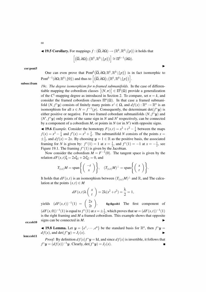
68
! 19.5 Corollary. For mappings f : (",#")$ (Rk,Rk\{p}) it holds thatA!
",#"";!Rk,Rk\{p}
"B4= >k!1(#").
"cor:pont5
One can even prove that Pontk!",#";Rk,Rk\{p}
"is in fact isomorphic to
Pontk!1(#";Rk\{0}) and thus toA!
",#"";!Rk,Rk\{p}
"B.
subsec:fram19c. The degree isomorphism for n-framed submanifolds. In the case of differen-tiable mapping the cobordism classes
.(N,v)
/# >k(") provide a generalization
of the C1-mapping degree as introduced in Section 2. To compare, set n = k, andconsider the framed cobordism classes >n("). In that case a framed submani-fold (N, f *y) consists of finitely many points x j # ", and d f (x) : Rn $ Rn is anisomorphism for all x # N = f!1(p). Consequently, the determinant det( f *y) iseither positive or negative. For two framed cobordant submanifolds (N, f *y) and(N%, f *y) only points of the same sign in N and N% respectively, can be connectedby a component of a cobordism M, or points in N (or in N%) with opposite signs.! 19.6 Example. Consider the homotopy F(x, t) = x2 + t2! 1
4 between the mapsf (x) = x2! 1
4 and f %(x) = x2 + 34 . The submanifold N consists of the points x =
±12 , and d f (x) = 2x. By choosing y = 1 # R as the positive basis, the associated
framing for N is given by: f *(1) = 1 at x = 12 , and f *(1) = !1 at x = !1
2 , seeFigure 19.1. The framing f *(1) is given by the Jacobian.
Now consider the cobordism M = F!1(0). The tangent space is given by therelation dF(x, t)( = 2x(1 +2t(2 = 0, and
T(x,t)M = span
6+!tx
,C, (T(x,t)M)2 = span
6+xt
,C.
It holds that dF(x, t) is an isomorphism between (T(x,t)M)2 and R, and The calcu-lation at the points (x, t) #M
dF(x, t)!+
xt
,= 2!(x2 + t2) =
!2
= 1,
yields (dF(x, t))!1(1) =+
2x2t
,. fig:figcob1 The first component of
(dF(x,0))!1(1) is equal to f *(1) at x =±12 , which proves that w = (dF(x, t))!1(1)
is the right framing and M a framed cobordism. This example shows that oppositesigns can be connected in M. "ex:cob10
! 19.8 Lemma. Let y = {e1, · · · ,en} be the standard basis for Rn, then f *y =d f (x), and det( f *y) = Jf (x). "
lem:cob11Proof: By definition d f (x) f *y = Id, and since d f (x) is invertible, it follows that
f *y = (d f (x))!1y. Clearly, det( f *y) = Jf (x).
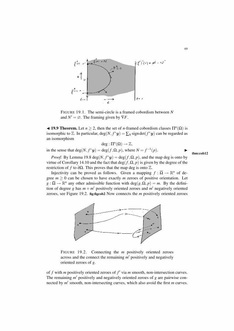
69
FIGURE 19.1. The semi-circle is a framed cobordism between Nand N% = !. The framing given by 9F .
! 19.9 Theorem. Let n, 2, then the set of n-framed cobordism classes >n(") isisomorphic to Z. In particular, deg(N, f *y) = $N signdet( f *y) can be regarded asan isomorphism
deg : >n(")$ Z,
in the sense that deg(N, f *y) = deg( f ,", p), where N = f!1(p). "thm:cob12
Proof: By Lemma 19.8 deg(N, f *y) = deg( f ,", p), and the map deg is onto byvirtue of Corollary 14.10 and the fact that deg( f ,", p) is given by the degree of therestriction of f to #". This proves that the map deg is onto Z.
Injectivity can be proved as follows. Given a mapping f : " $ Rn of de-gree m , 0 can be chosen to have exactly m zeroes of positive orientation. Letg : " $ Rn any other admissible function with deg(g,", p) = m. By the defini-tion of degree g has m + m% positively oriented zeroes and m% negatively orientedzeroes, see Figure 19.2. fig:figcob2 Now connects the m positively oriented zeroes
FIGURE 19.2. Connecting the m positively oriented zeroesacross and the connect the remaining m% positively and negativelyoriented zeroes of g.
of f with m positively oriented zeroes of f % via m smooth, non-intersection curves.The remaining m% positively and negatively oriented zeroes of g are pairwise con-nected by m% smooth, non-intersecting curves, which also avoid the first m curves.
70
These m+m% non-intersecting, smooth curve form M = F!1(p), for some smoothhomotopy F , and is a framed cobordism between N = f!1(p) and N% = g!1(p).The case m' 0 follows along the smae lines.
For n = 1, there are three framed cobordism classes, characterized by the func-tions f (x) = x, f (x) = !x, and f (x) = 1 respectively, and deg is an isomorphismfrom >1(") to the set {!1,0,1}.! 19.11 Exercise. Prove the above statement for n = 1. "exer:cob13
Using the characterization of the mapping degree in terms of the boundary re-striction, Theorem 19.9 shows that if two mappings 4,4% : #" $ Sn!1 have thesame the degree, then their extension to " yield the same framed cobordism class,and therefore the same homotopy type. This proves Lemma 14.5.subsec:gr119d. The group structure of framed cobordism classes and cohomotopy groups.Define the group operation on >k!1 and explain the link to cohomotopy groups.In the case of k = n the degree is rediscovered. If computable these algebraic in-variants are useful for studying the extension problem. The Pontryagin manifoldsand framed cobordisms are a differentiable tool for studying cohomotopy. Com-pare the proof in the previous subsection and the cobordism proof of the homotopyinvariance of degree.

71
V. The Leray-Schauder degree
ch:LSA natural question to ask is if there exists a degree theory for mappings on
infinite dimensional spaces? The answer to this question is not so straightforwardas the following example will show. Consider the space of sequences defined by!2 := {x = (x1,x2, · · ·) | $i x2
i < %}. The space !2 4= R% has a natural norm +x+2!2 :=
$i x2i and inner product (x,y) := $i xiyi and is a complete normed space, called a
Hilbert space. Let B% = {x # !2 | +x+!2 ' 1} and define a mapping f as follows:
f (x) =)D
1!+x+2!2 ,x1,x2, · · ·
*,
which is a continuous mapping from B% to #B% =: S%. It follows that f has no fixedpoints in B%. Indeed, for x# S% it holds that f (x) = (0,x1,x2, · · ·) -= x. On the otherhand f (B%) " B% and the mapping f satisfies the requirements of the Brouwerfixed point theorem, which therefore does not holds for continuous mappings ofon !2. If a degree theory for continuous maps on !2 exists so does the Brouwerfixed point theorem. This is already an indication that a degree for continuousmappings on infinite dimensional spaces does not exist. More precisely, followingthe proof of the Brouwer fixed point theorem, define r(x) = x + !!(x)( f (x)! x),where !!(x)' 0. Since r|S% = Id the homotopy property of the degree yields that
deg(r,B%,0) = deg(Id,B%,0) = 1,
which implies that r(x) = 0 has a non-trivial solution. On the other hand, sincef has no fixed points it holds that r(B%) = S%, which is a contradiction with theexistence of a degree theory,
Another consequence of the above construction is that any two mappings g1,g2from S% to S% are homotopic. Indeed, h(x, t) = r
!(1! t)g1(x) + tg2(x)
"12 givesa homotopy bewteen g1 and g2. If g1 = Id then deg(g1) = 1 and if g2 = f thendeg(g2) = 0, which implies degree cannot characterize homotopy classes. In par-ticular S% is contractible. This is far from the situation in finite dimensions.
The goal of this chapter is to find an adequate degree theory for the infinitedimensional setting and to extend the theory of homotopy classes of maps from Rn
to Rn to homotopy classes of maps on infinite dimensional spaces.
20. Notationsec:not2
The infinite dimensional spaces under consideration in this chapter are normedlinear vector spaces are their subsets. Extensions will be discussed in the nextchapter. Let X be a (real) linear vector space. On X we define a norm + ·+X , or + ·+for short which satisfies the following hypotheses:
12One easily verifies that +(1! t)g1 + tg2+2!2 ' 1 provided +gi+2
!2 = 1, i = 1,2.
72
(i) +x+ y+ ' +x+++y+, for all x,y # X ,(ii) +!x+= |!|+x+, for all x # X , and for all ! # R,
(iii) +x+= 0 if and only if x = 0.If there is no ambiguity about the space involved we simply write + ·+.
The combination (X ,+ ·+) is called a normed linear vector space. If in additionX is complete it is called a Banach space. A normed linear space is completeif every Cauchy sequence has a limit in X ; {xn} " X , with +xn ! xm+ $ 0, asn,m $ %, implies that there exists a x # X such that +xn ! x+ $ 0, as n $ %.Normed vector spaces and Banach spaces are examples of metric and completemetric spaces respectively, where the metric is given by
d(x,y) := +x! y+.
For the remainder of this chapter X is assumed to be complete, i.e. a Banach space.As in the previous chapter " " X denotes an open and bounded subset of X .
The closure in X is denoted by " and the boundary is given by #" = "\".subsec:continuity
20a. Continuity. Throughout this section X , and Y are (real) Banach spaces withnorms + ·+X and + ·+Y respectively. We omit the subscripts is there is no ambiguityabout the notation.
! 20.1 Definition. A mapping f : X $ Y is continuous if xn $ x (in X) impliesthat f (xn)$ f (x) (in Y ). A map is uniformly continuous on X , if for for any & > 0there exists a '& > 0 such that +x! y+ < ' implies that + f (x)! f (y)+ < &. Thelatter can also be defined with respect to a closed subset A" X . "
defn:cont1A continuous function f : X $ Y is bounded if f ("%) " X is bounded for any
bounded subset "% " X . Continuous mappings on Rn are necessarily bounded, i.e.bounded sets in Rn are mapped to bounded set under f . This is however not thecase in general Banach spaces.! 20.2 Exercise. Give an example of continuous map between Banach spaces that is notbounded. "exer:count1
! 20.3 Lemma. A uniformly continuous map is bounded. "lem:cont2
Proof: We need to show that for any bounded set A" X the image f (A)" Y isalso bounded. Choose R > 0 such that A " BR(0), and let n > 2R
' . Then for anytwo points x,y # A it holds that +x! y+ ' 2R, and one can define the line-segmentxt = x + t(y! x), t # [0,1], in BR(0). For ti = i
n we obtain point xti " BR(0), with+xti !xti+1+< ', by the choice of n. Since f is uniformly continuous it follows that+ f (xti)! f (xti+1)+< &, for all i. From the triangle inequality we then get
+ f (x)! f (y)+ '$i+ f (xti)! f (xti+1)+< n&,
which proves the boundedness of f .
The space of continuous mappings from X to Y is denoted by C0(X ,Y ) andthe bounded continuous maps by C0
b(X ,Y ). For mappings on bounded domainsf : "" X $ Y we write f #C0(";Y ) or C0(") in the case that X = Y . The space
73
of bounded continuous functions on " is denoted by C0b(";Y ), or C0
b("). On C0b
the following norm is defined
+ f+C0b
:= supx#"
+ f (x)+Y ,
which makes C0b(") a normed linear space.
subsec:diffbty
20b. Differentiability. ! 20.4 Definition. A mapping f # C(X ,Y ) is calledFrechet differentiable at a point x0 # X , if there exists a bounded linear mapA : X $ Y such that
+ f (x)! f (x0)!A(x! x0)+= o(+x! x0+),
in a neighborhood N of x0. "defn:diff1
We use the notation A = f %(x0) for the Frechet derivative. If the map x 1$ f %(x) iscontinuous as a map from X to B(X ,Y ), then f is of class C1; notation f #C1(X ,Y ).
! 20.5 Definition. A mapping f #C(X ,Y ) is called Gateaux differentiable in thedirection h # X , at a point x0, if there exists a y # Y such that
limt$0
+ f (x0 + th)! f (x0)! ty+= 0,
with x0 + th defined in a neighborhood N of x0. "defn:diff2
The Gateaux derivative at at point is usually denoted by d f (x0,h) and is com-monly referred to as the directional derivative in the direction h. In Rn is notion isknown as partial derivative and is a weaker notion of differentiability.! 20.6 Exercise. Give an example of a function that is Gateaux differentiable in a point,but is not Frechet differentiable. " exer:diff2
For functions on Rn there is an important relation between the two notions ofdifferentiability, i.e. the partial derivatives exist and are continuous, then the func-tion is differentiable. In the Banach space setting the same result holds.Theorem 20.7. If f # C(X ,Y ) is Frechet differentiable at a point x0, then f isGateaux differentiable at x0. Conversely, if a function f # C(X ,Y ) is Gateauxdifferentiable at x0 for all directions h#X, and the mapping x 1$ d f (x, ·)#B(X ,Y )is continuous at x0, then f is Frechet differentiable at x0. thm:diff3
In the latter case we write, by the linearity of d f in h, that d f (x,h) = d f (x0)h =f %(x)h.
Proof: The first claim of the theorem simply follows from the definition of theFrechet derivative. For the converse we argue as follows. By assumption the mapf (x0 + th) is differentiable in t (sufficiently small), and d f (x0 + th,h) = d f (x0 +th)h is continuous in t. Therefore,
f (x0 +h)! f (x) =Z 1
0d f (x0 + th)hdt.
74
Using this identity we find the following estimate:
+ f (x0 +h)! f (x0)!d f (x0)h+ = +Z 1
0
!d f (x0 + th)!d f (x0),h
"dt+
'Z 1
0+!d f (x0 + th)!d f (x0),h
"+dt
'Z 1
0+d f (x0 + th)!d f (x0)+B(X ,Y )+h+X dt
= o(+h+),by the continuity of d f (x0 + th).
The notions differentiability can be further extended to higher derivatives and weleave this to the reader. Furthermore, one can easily prove various basic propertiesof derivatives:! 20.8 Exercise. Prove the chain rule: Let f : X $ Y , g : Y $ Z, and f and g are differen-tiable at x0 and y0 = f (x0) respectively. Then
!g( f (x0))
"% = g%( f (x0)) · f %(x0). "exer:diff4! 20.9 Exercise. Prove the product rule: Let f : X $ R, and g : X $Y be differentiable atx0, then f ·g is differentiable at x0, and ( f ·g)%(x0)h = f %(x0)h ·g(x0)+ f (x0) ·g%(x0)h. "exer:diff5
A value p # Y is called a regular value if f %(x) # B(X ,Y ) is surjective for allx # f!1(p) and p is singular, or critical if it is not a regular value. A point x # Xis called regular if f %(x) is surjective and otherwise a point is called singular, orcritical point.
subsec:fred120c. Fredholm mappings and proper mappings. Let f be a C2 proper Fredholmmapping of index 0.
Important! Mention the Kuiper result
21. Compact and finite rank mapssec:compact
An important subspace of continuous mappings are the compact mappings fromf : X $ X . A mapping f : X $ X is compact if f ("%) is compact for any boundedsubset "% " X . Compact mappings are bounded since f ("%) is bounded for anybounded set +% " X . The space of compact mappings on X is denoted by K(X).This definition of compact mappings also holds for continuous mappings on sub-sets of X .
! 21.1 Definition. A continuous map k : "" X $ X is called compact if k(") iscompact. "
defn:comp1In particular for any "% "" it holds that f ("%) is compact since f ("%)" f (").
The space of compact mappings on " is denoted by K(") " C0b("). Compact
maps are examples of mappings which are close to mappings in finite dimensionalEuclidean space. The following lemma explains how compact maps can be approx-imated by maps of finite rank. To be more precise, a finite rank map is a mappingwhose range is contained in a finite dimensional subspace of X . The subspace offinite ranks mappings is denoted by F(";X)"C0(";X).

75
! 21.2 Lemma. Let k # K("), then for any & > 0, there exists a finite rank mapk& # F(") such that +k! k&+C0
b< &. i.e. k& # F(").C0
b("). "lem:finrank1
Proof: Since k(") is compact it can be covered by finitely many balls B&(xi),with xi # k("). Define
µi(x) =!i(x)
$ j ! j(x),
where !i(x) = max(0,&!+k(x)! xi+). This maximum is zero whenever k(x) -#B&(xi) and therefore µi(x) = 0, unless +k(x)! xi+< &. Set
k&(x) = $i
µi(x) · xi.
Now k&(")" span(xi). As for the approximation we obtain
+k! k&+C0b=
EEk!$i
µi · xiEEC0
b=
EEE$i
µi · (k! xi)EEE
C0b
,
using the fact that $i µi = 1. By construction +µi(x)(k(x)! xi)+< µi& and thus
+k! k&+C0b
= supx#"
EEE$i
µi(x)(k(x)! xi)EEE
' supx#"
$i
EEEµi(x)(k(x)! xi)EEE < $
iµi(x)& = &,
which completes the proof.
The converse of this lemma can be formulated as follows:
! 21.3 Lemma. For any sequence {k&} " F(").C0b("), with k& $ k in C0
b("),as &$ 0, it holds that k # K("). "
lem:finrank2Finally, using the above characterization of compact mappings, it is worth men-
tioning a version of Tietze’s extension theorem for compact mappings.
! 21.4 Lemma. Any compact mapping f # K(") extends to a compact mappingf # K(X). "
lem:finrank3
! 21.5 Lemma. Let k # K(").C1("), then for any x # " the linear operatork%(x) : X $ X is compact. "
lem:finrank4Proof: Under construction.
22. Definition of the Leray-Schauder degreesec:LSdeg
The problem with degree theory in infinite dimensional spaces is that homotopyinvariance, a basic property of the degree, prevents the existence of a non-trivialdegree theory (compare the axioms for degree theory, Section 7). We can alter thenotion of homotopy invariance in order to build a degree theory, or limit the types
76
of maps for which a degree is well-defined. The Leray-Schauder degree does bothby considering specific types of mappings, namely mappings of the form
f = Id! k,
where Id is the identity map on X and k # K("). Homotopies are considered in thesame class. Denote the function class by C0
Id(") = { f = Id!k | k # K(")} and byC0
Id(X) for mapping defined on X . These classes are affine subspaces of C0b(") and
C0b(X) respectively.
The set #" is a closed and bounded set in X . Due to the specific form of f the setf (#") is also closed and bounded. Indeed, let xn # #" such that f (xn)$ x*. Sincek is compact we have that k(xn) has a convergent subsequence and k(xnk)$ x**.Therefore, xnk = f (xnk)+ k(xnk)$ x*+ x** = x, which, by continuity, implies thatx* = x! k(x) = f (x), proving the closedness of f (#"). For the boundedness weargue as follows: k(#") is pre-compact and thus f (#") is bounded. Combiningthese facts we conclude that p -# f (#") implies that
infx##"
+p! f (x)+= infy# f (#")
+p! y+= ' > 0.
Indeed, if not, there exists a minimizing sequence xn # #" such that f (xn) $ p.By the closedness of f (#") then p # f (#"), a contradiction.
! 22.1 Definition. Let f be a continuous map of the form f # C0Id("), and let
p -# f (#"). Let k& be a finite rank perturbation with +k!k&+C0b< & and & < '/2 (' as
given above) and with k&(")"Y & " X (subspace). Then for any finite dimensionalsubspace X& containing both Y & and p, define the Leray-Schauder degree as
degLS( f ,", p) := deg( f &,".X&, p),
where f & = id! k&. If there is no ambiguity about the context we mostly omit thesubscript for the notation. "
defn:LSdegThe remainder of this section is devoted to showing that the Leray-Schauder
degree is well-defined. By the choice of domain ".X& it follows that f : ".X& $X& and p # X&. Moreover, p -# f &(#".X&),13 which follows from the followinginequality:
infx##".X&
+p! f &(x)+ = infx##".X&
+p! x+ k&(x)+ , infx##"
+p! x+ k&(x)+
, infx##"
+p! x+ k(x)+!'/2 > '/2 > 0.
The degree d( f &,".X&, p) is well-defined. We show now that the definition isindependent of the chosen subspace X& and approximation k&.

77
! 22.2 Lemma. Let -X& " X be any finite dimensional subspace such that Y & " -X&
and p # X&. Then deg( f &,". -X&, p) = deg( f &,".X&, p). "lem:dim1
Proof: Step (i): Consider mappings of the form g = Id! h : D " Rn:Rm $Rn:Rm, with h(D) " Rn. Suppose p # Rn and p -# g(#D). Then, deg(g,D, p) =deg(gn,D.Rn, p), where gn = g|D.Rn . We prove the above statement in the casethat h is C1, since the degree is defined via C1 approximations and with p = 0by virtue of the Property (v) in Section 7. Let "1 and "2 be top forms on Rn
and Rm respectively withRRn "1 =
RRm "2 = 1 and their supports contained in a
sufficiently small neighborhood of the origin. In terms of coordinates we writex = x1 + x2, x1 # Rn and x2 # Rm. For the degree this yields
deg(g,D, p) =Z
Dg*("18"2)
=Z
D+1(x1!h(x1 + x2))+2(x2)Jg(x1 + x2)dx1dx2.
By the specific form of g we have that Jg(x1 + x2) = det)
Id! #h#x1
(x)*
. Since theexpression for the degree is independent of "1 and "2 we can choose +2 to approx-imate a density function that peaks at 0 and has integral equal to 1 — approximatinga delta distribution. Due to the independence on +2 this gives
deg(g,D, p) =Z
D.Rn+1(x1!h(x1))det
+id! #h
#x1(x1)
,dx1,
= d(gn,D.Rn, p).
Step (ii): Since Y & " X& . -X& and p # X& . -X& we may assume without loss ofgenerality that X& " -X&. By construction it holds that f & : ".X& $ X& and f & :". -X& $ -X&. Consider the linear change of variables y = q(x) such that q(X&) =Rn:0 and q(-X&) = Rn:Rm. Then g = q7 f & 7q!1 = Id!h and h(D) " Rn:0,where D = q(". -X&) " Rn :Rm. From Step (i) it follows that deg(g,D, p) =deg(gn,D.Rn, p). It remains to prove that the degree is invariant under the changeof coordinates. Using differential calculus and the integral characterization of thedegree we obtain:
Z
Dg*" =
Z
D(q7 f & 7q!1)*" =
Z
D(q!1)*
!( f &)*(q*")
"
= sign)
Jq!1(x)*Z
".-X&( f &)*(q*")
= sign)
Jq!1(x)*
deg( f &,". -X&, p)Z
Rn+mq*"
= sign)
Jq!1(x)*A
deg( f &,". -X&, p)Bsign
)Jq(y)
*Z
Rn+m"
= deg( f &,". -X&, p)Z
Rn+m".
13For a linear subspace X& " X it holds that #(".X&) = #".X&.

78
SinceR
D g*" = deg(g,D,q(p))RRn+m " it follows that
deg(g,D,q(p)) = deg( f &,". -X&, p),
which proves that the degree is invariant under coordinate changes. By restrictingto the subspace & we obtain deg(gn,D.Rn,q(p)) = deg( f &,".X&, p). The prooffollows now from Step (i).
The final step in showing that Definition 22.1 proposes a well-defined notionof degree, is to prove that for & < '/2 the definition is independent of the chosenapproximation k&.
! 22.3 Lemma. Let k& and k& both be finite rank approximations for k with +k!k&+C0
b< & , +k! k&+C0
b< & and & < '/2. Then
deg(Id! k&,".X&, p) = deg(Id! k&,". -X&, p),
for any subspaces X& and -X& containing both p and the ranges of k& and k& respec-tively. "
lem:dim2Proof: Let Z& " X be a finite dimensional linear subspace containing both X&
and -X&. From Lemma 22.2 it follows that
deg(Id! k&,".X&, p) = deg(Id! k&,".Z&, p),deg(Id! k&,". FX&, p) = deg(Id! k&,".Z&, p).
Consider the compact homotopy k&t = (1! t)k& + tk&. which yields a homotopy
f &t = Id!k&
t and is a proper homotopy. By Property (ii) of Section 7 then deg(Id!k&,".Z&, p) = deg(Id! k&,".Z&, p) which then proves that
deg(Id! k&,".X&, p) = deg(Id! k&,". -X&, p).
The Leray-Schauder degree is well-defined.
23. Properties of the Leray-Schauder degreesec:props2
The properties of the (Brouwer) degree listed in Section 7 hold equally well forthe Leray-Schauder degree. For this list we refer to Section 7. For proving theseproperties for the Leray-Schauder degree one has to make sure that approxima-tions are constructed such that the conditions for the Brouwer degree are met. Animportant property is the validity property. If p -# f ("), then degLS( f ,", p) = 0.This is proved as follows. Due to the form of f the set f (") is closed and sincep -# f (") we have that infy# f (") +p! y+ , ' > 0. Let f & be an approximation forf as described in the definition of the Leray-Schauder degree (Definition 22.1) andwith X& such that f &(") " X& and p # X&. If we choose & > 0 small enough,i.e. & ' '/2, then for all + f ! f &+Cb
0< & it holds that infy# f &(".X&) +p! y+ ,
infy# f (") +p! y+! '/2 , '/2 > 0 and p -# f &(".X&). From the properties ofthe Brouwer degree we now have that deg( f &,".X&, p) = 0. As an immediateconsequence it now holds that
degLS( f ,", p) -= 0,

79
implies that f!1(p) -= !. Indeed, if f!1(p) = !, then dLS( f ,", p) = 0, a contra-diction.
Another way to treat the Leray-Schauder degree is to show that the axioms ofa degree theory are satisfied and derive the properties from that. We start with theLeray-Schauder degree theory and explain the axioms in a more general contextlater on.
Consider triples ( f ,", p) with "" X a bounded and open set in a Banach space(X ,+ ·+ ), f # C0
Id(") and p # X\ f (#"). For such triples we assign the Leray-Schauder degree
( f ,", p) 1$ degLS( f ,", p).
! 23.1 Theorem. For Leray-Schauder degree we have the following properties:(A1) if p #", then degLS(Id,", p) = 1;(A2) for "1,"2 " ", disjoint open subsets of ", and p -# f
!"\("1 /"2)
", it
holds that degLS( f ,", p) = degLS( f ,"1, p)+degLS( f ,"2, p);(A3) for any continuous paths t 1$ ft = Id! kt , kt # K(") and t 1$ pt , with pt -#
ft(#"), it holds that degLS( ft ,", pt) is independent of t # [0,1];and degLS is called a degree theory. "
thm:propsLSProof: Under construction.
As in the case of the Brouwer degree the essential properties of the Leray-Schauder degree follow from (A1)-(A3). In Section 7 we choose to prove theseproperties of the degree using only the axioms. Therefore most properties holdalso for the Leray-Schauder degree with the same proofs. There are some differ-ences though. Let us go through the list in Section 7 and point out the differences.
! 23.2 Property. (Validity of the degree, Property 7.4) If p -# f ("), thendegLS( f ,", p) = 0. Conversely, if degLS( f ,", p) -= 0, then there exists a x # ",such that f (x) = p. "
pt:prop1LS! 23.3 Property. (Continuity of the degree, Property 7.5) The degree degLS( f ,", p)is continuous in f = Id! k, i.e. there exists a ' = '(p, f ) > 0, such that for allg = Id! k satisfying +k! k+C0
b< ', it holds that p -# g(#") and deg(g,", p) =
deg( f ,", p). "pt:prop2LS
! 23.4 Property. (Dependence on path components, Property 7.6) The degree onlydepends on the path components D" X\ f (#"), i.e. for any two points p,q # D"X\ f (#") it holds that degLS( f ,", p) = degLS( f ,",q). For any path componentD" X\ f (#") this justifies the notation degLS( f ,",D). "
pt:prop4LS! 23.5 Property. (Translation invariance, Property 7.7) The degree is invari-ant under translation, i.e. for any q # X it holds that degLS( f ! q,", p! q) =degLS( f ,", p). "
pt:prop5LS
80
! 23.6 Property. (Excision, Property 7.8) Let 6 " " be a closed subset in " andp -# f (6). Then, degLS( f ,", p) = degLS( f ,"\6, p). " pt:prop6LS! 23.7 Property. (Additivity, Property 7.9) Suppose that "i " ", i = 1, · · · ,k,are disjoint open subsets of ", and p -# f
!"\(/i"i)
", then degLS( f ,", p) =
$i degLS( f ,"i, p). "pt:prop7LSAs for the Brouwer degree the Leray-Schauder degree can also be defined in the
C1-case. Let p#X\ f (#") be a regular value then by the Inverse Function Theoremthe set f!1(p) consists of isolated points. Let xn # f!1(p), then xn = p + k(xn)which has a convergent subsequence by the compactness of k and therefore f!1(p)is compact. Combined with isolation this yields that f!1(p) is a finite set. Usingthe excision and additivity Properties 23.6 and 23.7 we derive that degLS( f ,", p) =$ j degLS( f ,N&(x j), p), x j # f!1(p). It holds that
degLS( f ,N&(x j), p) = degLS( f ,B&%(x j), p) =: i( f ,x j),
for all for any 0 < &% sufficiently small. The integer i( f ,x j) is called the index of anisolated zero. For the Brouwer degree the index is given by the sign of the Jacobianat x j. Since for each x# f!1(p) the operator f %(x) = I!k%(x)#B(X)14 is invertiblede index given by the following spectral formula. Let ! > 1 be an eigenvalue ofA = I! k%(x), i.e. A( = !(, X 6 ( -= 0, then
n! = dim
=%[
k=1ker(!I!A)k
>< %,
by the compactness of k%(x).
! 23.8 Lemma. Let x #" be a regular point of f = C0Id("), then
i( f ,x) = (!1)*,
where * = $!>1 n!. "lem:id2
Proof: Under construction.
! 23.9 Remark. The formula for the index can also be given for the Brouwer degreebecause (!1)* = sign(Jf (x)) is the finite dimensional case. The above considera-tion also show how the Leray-Schauder degree is defined axiomatically and leadsto a similar expression as a sum of indices in the C1-case. The latter can also beused as a first definition. "rmk:id2
24. Compact homotopiessec:comphom
Corollary 15.2 relates the existence of a zero of any extension f : B1(0)$ Rk
of f |#B1 to the homotopy type of the 4 = f /| f | : #B1 = Sn!1 $ Sk!1, i.e. a non-trivial zero exists if and only if [4] # 3n!1(Sk!1) is non-trivial. The example inthe introduction showed that the infinite dimensional version of this result does nothold true without an appropriate notion of homotopy type. A mapping f : #B1 $
14The identity operator x 1$ x is denoted by Id and it linearization by I.

81
Rk\{0} that admits an extension f : B1 $ Rk for which f -= 0 is called inessentialwith repect to B1. Otherwise f : #B1(0)$Rk\{0} is called essential with respect toB1, i.e. every continuous extension f : B1 $ Rk has the property that f!1(0) -= !.
Let ""X be a closed and bounded subset and F : X $Y a continuous mapping.
! 24.1 Definition. Two mappings f ,g : ""X $Y are said to be compactly homo-topic relative to F is there exists a family of compact mappings k(t, ·) : "" X $Y ,t # [0,1], such that
(i) h(t,x) = F(x)+ k(t,x);(ii) h(0,x) = F(x)+ k(0,x) = f (x);
(iii) h(1,x) = F(x)+ k(1,x) = g(x).The associated compact homotopy classes are denoted by [ f ]c. "
defn:comphom1Using the Leray-Schauder degree we have the following analogue of Theorem
14.8 and Corollary 14.13 in the case that " " X is a bounded and convex domainand Y = X . As before the Leray-Schauder degree only depends on the boundarybehavior of a mapping and for a mapping 5 # C0
Id(#";X\{0}) we define
degLS(5) := degLS( f ,",0),
for any continuous extension f : "" X $ X .
! 24.2 Theorem. Let "" X be a bounded and convex domain.(i) Two mappings 50,51 # C0
Id(#";X\{0}) are compactly homotopy if and onlyif degLS(50) = degLS(51).
(ii) A mapping 5 # C0Id(#";X\{0}) is essential with respect to " if and only if
degLS(5) -= 0.In the latter case f (x) = 0 has a non-empty solution set for any continuous exten-sion f : "" X $ X of 5. "
thm:LS-equivProof: Under construction.
The Leray-Schauder degree classifies the homotopy classes and gives necessaryand sufficient consitions for the extension, or solvability problem (compare Section14). The restriction here is that " is convex. To extend the Leray-Schauder theoryand the results in Section 15 we start with mappings f : "" X $ Y , where Y " Xis a closed linear subspace of finite codimension. The function class with compactperturbations of a fixed inear Fredholm operator A : X $ Y is denoted by C0
A. Let5 # C0
A(#";\{0}), where range(5)" Y "Y , then considered as map into Y\{0} fis homotopically trivial. Indeed, degLS(5) = degLS( f ,",0) = 0. The latter followssince Y\ f (#") = Y\5(#") is path connected. In the case that " = B1(0) thefollowing result by Svarc generalizes the theory in Section 15.
In order to explain this extension we first discuss stable homotopy types. Westart with the Freudenthal suspension for maps between unit spheres Sn " Rn+1.Let 4 : Sn $ Sk be a continuous then the suspension operator defines an operatorS4 : Sn+1 $ Sk+1. Let f : Dn+1 " Rn+1 $ Rk+1 be any continuous extensionof 5. then define f : Dn+2 " Rn+2 $ Rk+2 by f (x,xn+2) := ( f (x),xn+2). Now
82
set S4 = f /| f | by restricting to Sn+1 and S4 : Sn+1 $ Sk+1. It follows from theconstruction that [S4] only depends on [4] and S : 3n(Sk) $ 3n+1(Sk+1) definesan isomorphism. This construction allows to define the notion of stable homotopytype.
! 24.3 Theorem. Let " = B1(0) and let A # B(X ,Y ) be a Fredholm operator ofindex !, 0. Then the homotopy classes of mappings 5# C0
A(#";Y\{0}) are givenby the stable homotopy groups 3n+!(Sn), n > !+1. "
thm:LS-equiv2Proof: Under construction.
In the case that Y = X and A = Id the stable homotopy is given by the Leray-Schauder degree.
! 24.4 Theorem. Let " = B1(0) and let A # B(X ,Y ) be a Fredholm operator ofindex ! , 0. Then the mapping 5 # C0
A(#";Y\{0}) is essential with respect to "if and only if [5]c corresponds to a non-trivial stable homotopy class in 3n+!(Sn),n > !+1. "
thm:LS-equiv3Proof: Under construction.
25. Stable cohomotopy
Describe the stable cohomotopy theory and the infinte dimensional framedcobordism theory. Explain some of the theory in Nirenberg, Berger and the pa-pers by Elworthy and Tromba.
26. Semi-linear elliptic equations and a priori estimatesapp2
In this section we will give a application of the Leray-Schauder degree in thecontext of nonlinear elliptic equations. We follow the notes by L. Nirenberg. Themethods that we discuss apply in general for elliptic differential operator of anyorder. In order to simplify matter here we will restrict ourselves to the Laplaceoperator with Dirichlet boundary data. Let D " Rn be a bounded domain withsmooth boundary #D. Consider the problem
!=u = g(x,u,9u), u = 0, x # #D.
For the nonlinearity g we assume that C%-function of arguments, i.e. g #C%(D&R&Rn), and
|g(x,u,9u)|'C +C|9u|0, 0 < 1,
uniformly in x #D, and u #R. Under these conditions we can prove the followingresult.Theorem 26.1. Under the assumptions on g the above elliptic equation has a so-lution u #C%(D). Moreover, if g(x,0,0) -; 0, then the solution u is not identicallyzero.
83
thm:PDE1Proof: The idea behind the proof is the formulate the above elliptic equation as
a problem of finding zeroes of an appropriate function f on a (infinite dimensional)Banach space. Let us start with choosing an appropriate space in which to work.Define X = H2.H1
0 (D) to be the intersection of two Sobolev spaces. For detailson Sobolev space we refer to the next chapter. We will use the implications ofthis choice with respect to the well-defined of the elliptic equation, and postponeto proofs to the next chapter. The space H2 .H1
0 is a Hilbert space with norm+u+X =
RD |=u|2dx. Due to the Dirichlet boundary conditions the Laplace operator
!= : H2 .H10 (D) " L2(D) $ L2(D) has a compact inverse (!=)!1 : L2(D) $
L2(D). We rewrite the elliptic equation as
(26.1) u! (!=)!1g(x,u,9u) = 0.
The above equation can be regarded as a seeking zeroes of the (Nemytskii) map- eqn:eq1ping f (u) = u! (!=)!1g(x,u,9u) on H2.H1
0 (D). By the estimate on g we havethat
Z
D|g(x,u(x),9u(x)|2dx ' C
Z
D
A1+ |9u(x)|20
Bdx
' C%)Z
D
A1+ |9u(x)|2
Bdx
*0
' C)
1++u+2H1
0
*0,
which proves that for u # X , g(x,u,9u)(x) is an L2-function. Consequently, thecomposition (!=)!1.g(x,u,9u)
/# X , proving that f : X $ X is well-defined. The
latter follows from the fact that R!(!=)!1" = H2 .H1
0 (D). As a map from L2 toH2 .H1
0 , the inverse Laplacian is an isometry. Concerning the continuity of thissubstitution map we refer to the next section. If we define Y = H1
0 (") then f is amap from Y to Y , and f = id! k, where k : Y $ Y is a compact map. Indeed, kis a composition of the Nemytskii map u 1$ g(x,u,9u) (from Y to L2), the inverseLaplacian (!=)!1 (from L2 to X), and the compact embedding X "$ Y , whichproves the compactness of k. This brings us into the realm of the Leray-Schauderdegree.
Suppose u # X is a solution of the equation (26.1), then the estimate ong(x,u,9u) can be used now to obtain an a priori estimate on the solutions.
+u+2Y ' C+u+2
X = C+g(x,u,9u)+2L2
' C)
1++u+2Y
*0,
which, since 0 < 1, implies that +x+Y ' R.! 26.2 Exercise. Prove the inequalities +u+L2 'C+u+X , and +u+H1
0'C+u+X , for all u# X.
" exer:estXDefine the domain " = B2R(0)" X . Clearly, f is a continuous map from " into
X , which is of the form identity minus compact. Due to the above a priori estimate

84
f!1(0)" BR(0), and 0 -# f (#"), and therefore the Leray-Schauder degree
dLS( f ,",0),
is well-defined.In order to compute this degree we consider the following homotopy:
ft(u) = u! t(!=)!1[g(x,u,9u)], t # [0,1].
Notice, for t # [0,1] we have via the same a priori estimates, that f!1t (0)" BR(0),
and therefore 0 -# ft(#") for all t # [0,1]. Homotopy invariance of the Leray-Schauder degree then yields
d( f ,",0) = d(id,",0) = 1,
which implies, by validity property of the Leray-Schauder degree, that f!1(0) -=!. Equation (26.1) thus has a solution u # Y . The equation yields u =(!=)!1[g(x,u,9u)] # X , which that the solution also lies in X .
To prove regularity we use a bootstrapping argument. The integral estimates ong can be adjusted to Lp-estimates. This gives, by the Sobolev embeddings that:
u # H1,p =< g(x,u,9u) # Lp =< u # H2,p =< u # H1,p% ,
where 1p% = 1
p !1n , provided n > p. This yields the recurrence relation
1pk+1
=1pk! 1
n.
We can repeat these recurrent steps until k times until 2(k +1) > n > 2k, and thenu # H2,pk , where pk = 2n
n!2k . Again by the Sobolev embeddings, we have that
H2,pk(D) "$C1,.(D),
where . = 1! npk
, since npk
= n2 !k, and k+1 > n
2 > k, it holds that 0 < . < 1. Wenow repeat the bootstrapping in the Holder space:
u #C1,. =< g(x,u,9u) #C0,0. =< u #C2,.% ,
where .% = 0.. The idea now is the use the elliptic regularity theory for the Lapla-cian be differentiation the equation. Let vi = #u
#xi, then
!=vi = #xig+(#ug)vi +$j
#v j g#v j
#xi.
Since g is a C%-function of its arguments, and u # C2,.% , the right hand side isin C0,.% , implying that vi # C2,.% , and thus u # C3,.% . We can repeat this processindefinitely, which proves that u #C%(D).
If g(x,0,0) -; 0, then u = 0 cannot be a solution, and thus u -; 0.

85
VI. Minimax methods
ch:minimaxIn this Chapter we discuss a first example of a class of methods, also referred to
variational methods, that are used to find critical points of functions on finite andinfinite dimensional spaces. The main characteristic is to link topological proper-ties of the space to the set of critical points of the function in question.
27. Palais-Smale functions and compactnesssec:PS
The following example shows that critical point theory can break down on vari-ous aspects of non-compactness. Consider the function f (x) = arctan(x). Clearly,f has no critical values, and thus no critical points on R. The values c = ±3/2are special however. One can for example take sequences {xn}, xn = ±n, suchthat f (xn)$ c and f %(xn)$ 0. Regardless of the fact that f % goes to zero alongsuch sequences there are no critical points. One could argue that there exist criticalpoints at ‘infinity’. This would require compactifying our setting.
This simple example already goes to show that due to the non-compactness ofR, the domain of definition of f , the notion of critical value and critical point lacksunform estimates. For this very reason Palais and Smale, in their work on Morsetheory in infinite dimensions, introduced the following compactness condition.
! 27.1 Definition. Let X be a (reflexive and separable) a Banach space. A functionf # C1(X ;R) is saidf to satisfy the Palais-Smale condition at c — (PS) for short—, if any sequence {xn}" X for which
f (xn)$ c, f %(xn)$ 0,
has a convergent subsequence. "defn:PS
This condition was referred to as ‘Condition (C)’ in the original work of Palaisand Smale. One can also require a function to satisfy (PS) for an interval of valuesc, i.e. a function satisfies (PS) on an interval I if it satsifies (PS) for every c # I.The same holds for the Palais-Smale condtion on X . In that case we do not specifyc beforehand.
The (PS) condition has various consequences for Palais-Smale functions. De-note by Cf (I) the set of critical points of f with critical values restricted to theinterval I.
! 27.2 Lemma. Let f #C1(X) satsify (PS) for some c, then the set Cf (c) is com-pact. Moreover, Cf (I) is compact whenever I is compact. "
lem:compact1Proof: Compactness is established by pointing out that compactness for a met-
ric space is equivalent to sequential compactness. The space (Cf (c),d) with the in-duced metric is a metric space itself. For any sequence {xn} we have that f (xn) = c,and f %(xn) = 0. The (PS)-condition then implies that xnk $ x # X . Consequently,
86
f (x) = c and f %(x) = 0, and thus x #Cf (c), which establishes sequential compact-ness. The same holds for Cf (I).
Another important consequence of the (PS)-condition is uniformity on lowerbounds for f % regular values.
! 27.3 Lemma. Let c be a regular value for f . Then there exists an & > 0, suchthat + f %(x)+X* , ' > 0 for all x # f!1[c! &,c+ &]. "
lem:lowerb1Proof: The fact that c is regular implies that a neighborhood [c! &,c + &], for
some & > 0, consists of regular values. If not, one can choose cn $ c, and xn,with f (xn) = cn, and f %(xn) = 0. By (PS) we have that xnk $ x, with f (x) = c andf %(x) = 0, a contradiction.
For any c* # [c!&,c+&] one can find a 'c* > 0 such that + f %(x)+X* , 'c* > 0 forall x # f!1(c*). Indeed, otherwise one can find sequences {xn} such that f %(xn)$0, which, by (PS), have convergent subsequences converging to a critical point atlevel c*, a contradiction.
Finally, 'c* , ' > 0 for all c* # [c!&,c+&], by repeating the above argument.
28. The deformation lemmasec:deform2
In this section we will start with a standard deformation result for sub-levelsets. In the previous section we explained that the Palais-Smale condition yieldsvarious properties for the sub-level sets f a := f!1(!%,a]. For sake of simplicitywe assume that X is a Hilbert space here with inner product (·, ·)X , or (·, ·) whenthere is no ambiguity about the space involved. In a Hilbert space one can definethe gradient of f via the relation
(9 f (x),y) = f %(x)y, = y # X .
The main tool in this is the following differential equation on X :dxdt
= ! 9 f (x)+9 f (x)+2 .(28.1)
The vector field on the right hand side is well-defined on regular level sets. Leteqn:ode1[a,b] be a interval of regular values of f , then by Lemma 27.3 we have that+9 f (x)+ , ' > 0, which make the above differential equation well-defined on thestrip f b
a := f!1[a,b]. Here we used the identity +9 f (x)+X = + f %(x)+X* .
! 28.2 Lemma. Let [a,b] be an interval of regular values of f . Assume that f #C2(X), and satisfies (PS) on the strip f b
a . Then f b is homotopically equivalent tof a, i.e. there exists a homotopy 1t : [0,1]& f b $ f b, such that
11( f b) = f a,
and 1t = id on f a. "lem:deform2
Proof: Consider Equation 28.1 with initial value x(0) = x # f ba , and denote
the solution by (t(x). From the theory of ordinary differential equation we know,since f #C2(X), that the solution (t(x) is well-defined for all x # f b
a by the aboveconsiderations.

87
! 28.3 Exercise. †† Prove the existence and uniqueness of (t in the above defined initialvalue problem. " exer:ode1
Consider the composition f 7(. Differentiating f 7( yieldsddt
f 7( = (9 f (((t)),(%(t)) =!1.
If we integrate this equation we obtain the following identity
f (((t))! f (x) =!Z t
0dt =!t,
and thus ( f 7 ()(t) = f (x)! t, which explains that f decreases along ((t). Usingthis identity we can now define a candidate for a homotopy that is well-defined forall x # f b.
(28.2) 1t(x) =
6(( f (x)!a)·t(x) for x # f b
a ,
x for x # f a.
! 28.4 Exercise. Verify that 1t is a homotopy as indicated in Lemma 28.2. " exer:homotopy1From Exercise 28.4 we have that 1t is a proper homotopy that deforms f b into
f a, which completes the proof.
! 28.5 Remark. In Lemma 28.2 we have chosen f to be of class C2 to ensure thelocal Lipschitz continuity of of the right hand side of Equation 28.1. In the litu-rature Lemma 28.2 is proved for C1-functionals by constructing so-called pseudogradient vector fields to play the role of 9 f . This way all the necessary propertiesfor the construction are preserved and the vector field is Lipschitz continuous. Herewe choose to leave out this technicallity for the sake of focussing on the main ideasinvolved. " rmk:smoothness1! 28.6 Remark. In the case f is invariant under a compact group action, i.e. if Gis a compact group and f (g(x)) = f (x), for all g # G, we get additional propertiesfor the deformations in Lemma 28.2. We have g(1t(x)) = 1t(g(x)), for all t, andall g # G.! 28.7 Exercise. Prove the above property for 1t . " exer:deform
This will be used later on to obtain multiplicity of critical points. " rmk:symmetryWe will now state a general version of the deformation lemma that is also used
in Morse theory in next chapter.Theorem 28.8. Assume that f # C2(X) satisfying (PS) on f b for some regularvalue b'%. Let c < b, and let N be a neighborhood of Cf (c). Then there exists an& > 0, and a 1-parameter semi-group of homeomorphisms ht : f b $ f b such that
(i) h0(x) = x,(ii) ht = id, if x #Cf , or if | f (x)! c|, &,
(iii) f (ht(x)) is non-increasing in t for all x # f b,(iv) h1( f c+&\N)" f c!&,(v) h1( f c+&)" f c!&/N.
88
In addition, if f is G-invariant with respect to some compact group G, then thehomeomorphisms ht are also G-invariant.
thm:deform3Note that if Cf (c) = !, then N can also be chosen to be the empty set.
29. The linking theorem and minimax characterizationssec:minimax
Our next step is explain how the classical minimax characterization of eigen-values can be generalized to finding critical points of functionals f #C2(X). Letus consider a simple example. Given the function f (x,y) = 1
2(x2 + y2)! 14 x4! y4.
Upon compute f % on find nine critical points, of which (±1,0) and (0,±2) are sad-dle points. For instance f (1,0) = 1
4 . This critical value has on more critical point,namely (!1,0), which is also a saddle point. The critical value can be thought offas a ‘mountain pass’, i.e. we start walking from the middle at (0,0) towards the‘outside’. Let us think of the surface given by f (x,y) as a mountain landscape.Standing at (0,0) is as being surrounded by a mountain range. We seek the bestway out, i.e. out of the valley, over the mountains, to the hinterland. The way to dothis is to seek a mountain passage. Starting at valley bottom at (0,0) we considerpaths {0(t)}t#[0,1] to a point where f (0(1)) < 0. Of all such paths we seek the mosteconomical one, i.e. the one for which f (0(t)) stays lowest. In mathematical terms:
c = inf0
maxt#[0,1]
f (0(t)).
By construction c > 0. We will explain now that c = 14 , and that in general such
characterizations lead to critical values and critical points.Let us review these ingredients again. Pick a point (x*,y*) such that f (x*,y*) <
0. Instead of considering arbitrary paths we restrict ourselves to paths connecting(0,0) and (x*,y*). Such a path then becomes a continuous map h from
Q = {(x,y) = t · (x*,y*), t # [0,1]},
to R2. The minimax described above is therefore
c = infh
max(x,y)#Q
f (h(x,y)).
The conclusion that c > 0 can be achieved by finding a second set S in R2
with the property that f |S , ' > 0, S .Q -=, and #Q . S = !. Here we cantake S = {(x,y) | x2 + y2 = 1}. Having these properties we know that c 'max(x,y)#Q f (x,y) < %. Since S.Q -= !, also S. h(Q) -= ! for any h. More-over, since #Q. S = !, it holds that max(x,y)#Q f (h(x,y)) , ' > 0. Summarizingthis yields that c > 0. The deformation lemma can now be used to prove that c isindeed a critical value. We will prove this idea in a more general setting.
We explain the general linking of set in X as introduced by Benci and Rabi-nowitz.

89
! 29.1 Definition. Let S " X be a closed subset, and Q is a finite dimensional(compact) submanifold in X with relative boundary #Q. The sets S and #Q link, orform a non-trivial link, in X if:
(i) S.#Q = !,(ii) h(Q).S -= !, for all maps h in the set
H = {h #C0(Q;X) : h|#Q = id}.
"defn:link1
The sets used in the mountain pass described above are of course examples oflinking sets, but one can also choose S to be a single point and Q a disc in X . Thenthe minimax decribes a local minimum for f . Let us now prove the main result ofthis section, and then given a few more examples of linking sets.
Theorem 29.2. Let f #C2(X), and let S and Q be as in Definition 29.1 — linkingsubsets in X. If infx#S f (x) > maxx##Q f (x), then the minimax
c = infh#H
maxx#Q
f (h(x)),
well-defined. Moreover, if f satisfies (PS) on [c!&,c+&], for some & > 0, then c isa critical value for f .
thm:linking1Proof: First, since S and #Q are linking sets, S and h(Q) intersect, and therefore
c , infx#S f (x) > maxx##Q f (x) > !%. On the other hand c ' supx#Q f (x) < %,which proves the well-definedness of c.
As for the critical value we argue by contradiction. Suppose c is a regular valuefor f . Since f satisfies (PS) for interval [c! &,c + &], for some & > 0, one canchoose an 0 < &1 < & such that
c! &1 > maxx##Q
f (x),
the interval [c!&1,c+&1] consists of regular values only. By Lemma 28.2 we havea homotopy 1t such that
11( f c+&1) = f c!&1 , and 1t = id on f c!&1 .
By the choice of &1 the map 11 restricted to Q has the property that 11|#Q = id.Indeed, since maxx##Q f (x) < c!&1, we have that #Q" f c!&1 , and thus 11 = id on#Q. Consequently, 11 #H. The latter implies that
infh#H
maxx#Q
f (h(x))' c! &1,
which is clearly a contradiction.

90
! 29.3 Remark. As pointed out before this general version of the linking can also bebe proved for C1-functions. In their work on minimax theory Benci and Rabinowitzintroduced the linking theorem in a broader context. Namely, in the general versionof Benci and Rabinowitz the set Q is allowed to be a submanifold modeled overan infinite dimensional set. This is very important for applications to stronglyindefinite problems such as Hamiltonian systems. To prove the general version ofBenci and Rabinowitz more groundwork is needed. Due to the infinite dimensionalnature of Q linking becomes a more delicate notion and the Leray-Schauder degreefor intersection theory is required. This then means that the set H of deformationsalso has to be altered. Without going into details the Benci and Rabinowitz theoremis for functions of the form f (x) = 1
2(Lx,x)X + b(x), where b is a function whosederivative is a compact mapping, and L is an isometry on X . This specific form isneeded to accommodate the Leray-Schauder degree theory. There are also versionsof Theorem 29.2 allowing infinite dimensional sets Q, and without f being of thespecific form as given above. Such results can be derived using Galerkin typearguments and require a slightly stricter version of the Palais-Smale condition. Inpractice this stricter version of (PS) is not a problem. "rmk:linking
Let us now give a couple of examples of linking sets. Our first example is adirect generalization of the mountain pass construction as sketched above.
Consider a decomposition X = X1:X2, with dimX2 < %. Define the sets
S = {x # X1 : +x+X = r},Q = {x = te+ x2 : e # X1, 0' t ' R1, x2 # X2, +x2+X ' R2}.
Under the assumption that 0 < r < R1, and 0 < R2, the sets S and #Q link.! 29.4 Exercise. Formulate S and Q in the case of the Mountain Pass Theorem, and showthat S and #Q link. "exer:exlink! 29.5 Exercise. Prove in the general case, using degree arguments, that S and #Q link."exer:exlink1
Our next example displays another class of linking sets. As before consider thedecomposition X = X1:X2, with dimX2 < %. Define the sets
S = X1, and Q = {x # X2 : +x+X ' R}.
Under the assumption that R > 0 the sets S and #Q link. Clearly #Q = {x #X2 : +x+X = R}, and thus S.#Q = ! In order to complete the proof that S and #Qlink we have have to show that S.h(Q) -= ! for any h #H. Let 3 be the projec-tion from X onto X2, then the intersection is non-empty if and only if 0 # 3h(Q).In terms of the degree this translates into d(3h,Q,0) -= 0. Consider the equation3h(x) = 0, with x # Q. Define the homotopy
ht(x) = t3h(x)+(1! t)x,
which connects id with 3h. By construction ht |#Q = id, and thus d(ht ,Q,0) is well-defined for all t # [0,1]. The homotopy invariance of the degree we then have that
d(3h,Q,0) = d(id,Q,0) = 1,

91
which completes our proof.The minimax principle explained in the linking theorem is based on a more min-
imax principle. A minimax theory consists of a function f #C2(X), and collectionA of subsets of X , and class of maps H, which have the property that for all A#A,and h #H it holds that h(A) #A. Define
c = infA#cA
supx#A
f (x).
The link f is given as follows: If c # R, then there exists an h #H, such that forsome sufficiently small & > 0 it holds that h( f c+&)" f c!&.Theorem 29.6. If f satisfies (PS) in the interval [c! &,c+ &] for some & > 0, thenc is a critical value of f . thm:mm1! 29.7 Exercise. Prove the above theorem. " exer:mm
In the chapter on applications we will apply the linking theorem to various el-liptic problems. To get multiplicity results additional information is needed. Ofcourse if one has two geometrically different minimax characterizations, but thefunction values c are the same, then there need not be two geometrically distinctcritical points. In next section we will adsress this question in more detail. AlsoChapter VII deals with multiplicity of critical points.
30. Ljusternik-Schnirelmann category and index theorysec:category
As pointed out in the previous section different minimax characterizations do notnecessarily yield different critical points. We start here with concept of categoryand the multiplicity theorem due to Ljusternik and Schnirelmann.
! 30.1 Definition. Let X be a complete metric space. A closed subset A " X issaid to be of category k relative to X — notation catX(A) = k — if;
(i) A" /ki=1Ai, with Ai " X closed and contractible in X ,
(ii) for any other union /lj=1A%j > A, with A%j " X closed and contractible in X , it
holds that l , k.The category is said to be infinite if no such coverings exist. "
defn:cat1The category is a topological invariant of X and can sometimes be easily com-
puted. There are also relations with other topological invariants such as homologyand co-homology.! 30.2 Exercise. Prove the following properties; (i); A,B " X, then catX (A / B) 'catX (A)+ catX (B), and (ii): A? B, then catX (A)' catX (B). " exer:cat2! 30.3 Exercise. Determine the Ljusternik-Schnirelmann category of Sn and T n. " exer:cat3
The Ljusternik-Schnirelmann category is a so-called index theory. An indextheory is a integer function on the class of closed subsets A" X which are invariantunder a compact group action, i.e. for some compact group G, g(A) = A for all g #G. For example let X = Rn, and consider G@ Z2 to be the group consisting of themaps {id,!id}. The set of closed sets A invariant under G are then characterizedby sets that reflection invariant with respect to the origin.
92
Denote the class of G-invariant closed subsets by A, and define H to be a closedsubset of the set of continuous maps h on X that commute with G, i.e. h7g = g7h.For G -= {id}, we define Fix(G) = {x # X : g(x) = x, =g # G}.
! 30.4 Definition. An index theory for (G,A,H) is a map i : A$ N/{%} satis-fying the following properties:
(i) i(A) = 0, A< A = !,(ii) A" B, =< i(A)' i(B),
(iii) i(A/B)' i(A)+ i(B),(iv) i(A)' i
!h(A)
", for all h #H,
(v) For A # A compact and A.Fix(G) = !, then i(A) < %, and there exists aneighborhood N #A of A, such that i(N) = i(A),
(vi) For x -# Fix(G) it holds that i!/g#G g(x)
"= 1.
"defn:ind1
! 30.5 Exercise. Show that the Ljusternik-Schirelmann theory is an index theory with G ={id}, A the class of all closed subsets of X, and H = C0(X ;X). "exer:ind2
Another example of an index theory is the Krasnoselskii genus. Consider theset A to be closed subsets of a Hilbert space X , satisfying A = !A. Choose G ={id,!id}, and H the set of odd maps. Define the genus as
0(A) = inf{m | Bh #C0(A;Rm\{0}), h(!x) =!h(x)},
and 0(A) = % if no h can be found for any m.! 30.6 Exercise. Show that 0 is an index theory for the triple (G,A,H) defined above. "exer:ind3
With the existence of an index theory one can prove the following general mul-tiplicity theorem in minimax theory. This theorem is for the case that f is boundedfrom below. One can also think about removing this restriction, which requires anextension of the notion of index theory. In the next theorem we assume that X isHilbert space. In the next theorem let A be the closed G-invariant subsets of f b forsome regular value b' %, and H the class of G-invariant homeomorphisms of f b.Theorem 30.7. Let f #C2(X) satisfying (PS) on f b for some regular value b'%,and let f be invariant with respect to some compact group G, i.e. f (g(x)) = f (x)for all g # G. Assume X is G-invariant, and Fix(G) = !. Let i be an index theoryfor (G,A,H), and define
Fi( f b) = sup{i(K) | K #A, compact}.
If f , !c on X, for some c , 0, then f admits at least Fi( f b) ' % geometricallydistinct critical points modulo G.thm:LS1
The above theorem also holds for complete Hilbert manifolds M embedded intoX . In this case we define to gradient vector field as the component in T M.
We start with defining minimax values. Define the subsets Ak of A as follows:
Ak = {A #A : i(A), k}.

93
For any k ' i(X) the sets Ak are non-empty, invariant under homeomorphismsh#H. Namely, by Property (iv) we have that k' i(A)' i(h(A)), Clearly, X "Ak,which proves that Ak -= !, for all k ' i(X). Now define the minimax values
ck = infA#Ak
supx#A
f (x).
! 30.8 Lemma. Let f # C2(X) satisfying (PS) on X , and let f be invariant withrespect to some compact group G. If
!% < ck < %,
then ck is a critical value for f . "lem:ind3
Proof: This proof follows along the same lines as the proof of Theorem 29.2.Suppose that ck is not a critical value of f , then there exists an & > 0 such that [c!&,c+ &] is an interval of regular values. Let A #Ak such that supx#A f (x)' c+ &%,&% < & sufficiently small. Then by Theorem 28.8 there exists an homemorphismh1 #H, such that k ' i(A)' i(h1(A)), and h1(A)" f c!&% . This then gives
ck ' c! &% < c,
a contradiction.
Clearly the values ck are critical for all k ' i(X). If they are all distinct, thenthey all correspond to different critical points. The question now is what happensif some of them are the same.
! 30.9 Lemma. Suppose
!% < ck = ck+1 = · · · = ck+l!1 = c < %,
then i(Cf (c)), l. "lem:ind4
Proof: We know from Lemma 30.8 that c is a critical value. The Palais-Smalecondition implies that the set Cf (c) is compact. By Property (v) (of index) thereexists a neighborhood N #A such that i(N) = i(A). As in the proof of the previouslemma we can choose a set A # Ak+l!1, such that f (x) ' c + &%, for all x # A.Clearly, by Theorem 28.8 h1(A) #Ak+l!1, and
h1(A)" f c!&% /N.
Since, for all A# Ak it holds that f (A) , c, and f ( f c!&) ' c! &, we have thatf c!& -#Ak, and thus
i( f c!&) < k,From the properties (ii) - (iv) we obtain: i(N) + i( f c!&) , i( f c!& /N), i( f c!& /N), i(h1(A)). Combining these estimates gives:
i(N) , i( f c!&/N)! i( f c!&)> i(h1(A))! k , i(A)! k, k + l!1! k = l!1.
Consequently, i(N) = i(Cf (c)), l, which proves the lemma.

94
Proof of Theorem 30.7: For any compact set K # A it holds that i(K) ' i( f b).Thus for all finite k ' i(K) ' supK i(K) = Fi( f b) the minimax values are boundedfrom above. The boundedness from below follows from the fact that f is boundedfrom below.
If all ck are different we obtain all distinct critical points. In the case of someck = · · · = ck+l!1 = c’s being the same Lemma 30.9 yields that i(Cf (c)) ' l > 1.Then there are at least l critical points. As a matter of fact by Property (vi) thenumber is infinite.
! 30.10 Remark. The statement in Theorem 30.7 can be inproved in the case of theLjusternik-Schnirelmann category. Assume cat f b( f b)) < %, then f b " /iAi (finitecovering). Then the set K = {xi}, xi # Ai, and xi -# A j, i -= j, is compact andcat f b(K) = cat f b( f b). Consequently, Gcat f b( f b) = cat f b( f b). When cat f b( f b) = %,then easily follows that supK cat f b(K) = %, proving that Gcat f b( f b) = cat f b( f b) ingeneral. Therefore,
|Cf ( f b)|, cat f b( f b),
for functionals that are bounded from below.In the case that a functional f is a bounded functional, i.e. for any bounded
set A, it holds that f (A) is a bounded interval, we can replace Fi( f b) by i( f b) inTheorem 30.7, so that |Cf ( f b)|, i( f b). "
rmk:LS2! 30.11 Remark. For functionals that are not bounded from above most of theminimax theory aplies, except for lower bounded in terms of the index. In that casewe need to resort to relative index theories. For instance for the category we canuse the relative category. We then get
|Cf ( f ba )|, cat( f b, f a)( f b),
which is explained in detail in []. "rmk:LS3
In this chapter the minimax and Morse theory will be applied to a model classof nonlinear elliptic differential equations. For our purposes here we are concernedwith elliptic problems of the form
!=u = g(x,u), x #",
u = 0, x # #",
where " " Rn is a bounded domain with smooth boundary #", and g(x,u) is aC%-nonlinearity that satisfies the growth estimate
|gu(x,u)|'C +C|u|p!1, p > 1,
uniformly in x # ", for all u # R. We will study solutions of this problem usingminimax and Morse theory. Standard regularity theory for this equation revealsthat solutions are C%("). Regularity issues will be postponed till later.
95
31. Variational principles and critical pointssec:varprin
As opposed to applying degree theory and fixed point arguments the equationabove possesses a alternative formulation for finding solutions; variational princi-ple. Consider the integral
Z
"
A12|9u(x)|2!G(x,u(x))
Bdx,
where G(x,u) =R u
0 g(x,s)ds. Clearly, the integral is well-defined for all u #C%(").C1
0("). Denote the integral as functional on functions u(x) by f . Let usconsider the first variation of the integral with respect to test functions 5 #C%
0 (").This yields
f (u+5)! f (u) =Z
"
A9u ·95!g(x,u)5
Bdx
+Z
"
A12|95|2!gu(x,u+25)52
Bdx.
As explained before, under the assumption that p < n+2n!2 , when n, 3, the function
f extends to the Sobolev space H10 (") = closH1(C%
0 (")), with equivalent norm
+u+H10
:=HZ
"|9u(x)|2dx.
This uses the compact embeddings
H10 (") "$
012
13
C0("), n = 1,
Lp+1("), n = 2, 0' p < %,
Lp+1("), n, 3, 0' p < n+2n!2 .
If we use the above variation formula we obtain that for fixed u # H10 (") it holds
that ;;; f (u+5)! f (u)!Z
"
A9u ·95!g(x,u)5
Bdx
;;; = o(+5+H10),
which proves that f is differentiable on H10 ("). Notation:
f %(u)5 =Z
"
A9u ·95!g(x,u)5
Bdx.
! 31.1 Exercise. Prove the above identity for the Frechet derivative in the case g(x,u) =!u+ |u|p!1u, using the first variation and the Sobolev emebeddings. "
exer:deriv1! 31.2 Exercise. †† In Section 28 we introduced the notion of gradient. Compute thegradient 9 f (u) in H1
0 ("). "exer:deriv1a
Similarly, the second variation yields;;; f %(u+4)5! f %(u)5!
Z
"
A94 ·95!gu(x,u)45
Bdx
;;; = o(+4+H10)+5+H1
0,
96
which proves that f twice continuously differentiable on H10 ("). Notation: Nota-
tion:
f %%(u)45 =Z
"
A94 ·95!gu(x,u)45
Bdx.
! 31.3 Exercise. Establish the expression for the second derivative in the case g(x,u) =!u+ |u|p!1u, by proving the identity for the second Frechet derivative. "
exer:deriv2The expression for the first derivative explains that the elliptic equation is sat-
isfied in a ‘weak’ sense, i.e. weak solution u # H10 ("). If additional regularity is
known then a simple integration by part provides the identityZ
"
A)!=u!g(x,u)
*5Bdx = 0,
for all 5 # H10 (", which reveals the equation again and u is a ‘strong’ solution.
This identity, without a priori regularity, can also be interpreted in distributionalsense, i.e. != is regarded as a map from H1
0 (") to its dual Sobolev space H!1(").
! 31.4 Exercise. Interpret the above identity in the dual space H!1("). "exer:weak1
Having established all these preliminary differentiability properties we concludethat solutions of the elliptic equation can be regarded as critical points of the func-tion f . This variational principle allows us to attack the elliptic problem via criticalpoint theory.
Before going to the actual application in the next section we first prove a resultconcerning the Palais-Smale condition.
! 31.5 Lemma. Let g and " be as above and let 1 < p < %, for n ' 2, and 1 <p < n+2
n!2 , for n, 3. In addition assume that for some 0 > 2,
0 < 0G(x,u)' ug(x,u), for |u|, r > 0.
Then, the function f satisfies the Palais-Smale condition on H10 ("). "
lem:PS1Proof: The requirements on p are needed in order for f to be well-defined and
differentiable. Let {un} be a sequence satisfying
f (un)$ c # R, and f %(un)$ 0,
as n$ % — a Palais-Smale sequence. In terms of the above integrals this reads:Z
"
A12|9un|2!G(x,un))
Bdx$ c, and
;;;Z
"
A9un ·95!g(x,un)5
Bdx
;;;' &n+5+H10, &n $ 0, =5 # H1
0 (").
97
! 31.6 Exercise. Derive the above inequalities from the definitions of f and f %. "exer:PS2The first step is to show that a Palais-Smale sequence {un} is uniformly bounded
in H10 ("), with the bound only depending on c. In the expression for the derivative
we choose 5 = 0!1un. This gives, upon substitution, that
!&n+un+H10
Z
"
A12|9un|2!g(x,un)un
Bdx' &n+un+H1
0.
Combining this inequality with the expression for f (un) we obtain:)1
2! 1
0
*Z
"|9un|2dx =
Z
"
AG(x,un)! 0!1ung(x,un)
Bdx
+ c+ &n + &n0!1+un+H10'C + 0!1&n+un+H1
0.
This inequality yields the estimate +un+H10'C.
Since H10 (") is a Hilbert space the boundedness of {un} implies that unk # u in
H10 ("). Since the embeddings of H1
0 (") into Lp+1(") are all compact, providedp < n+2
n!2 , n , 3, it holds that unk $ u in Lp+1. Consequently,R
" G(x,unk)dx $R" G(x,u)dx. If we combine this with the convergence of f we obtain:
12
Z
"|9un|2dx = f (un)+
Z
"G(x,unk)dx$ c+
Z
"G(x,u)dx,
which proves that +un+H10$+u+H1
0, and convergence of {unk} in H1
0 ("), complet-ing the proof.
Having establish the Palais-Smale condition for f allows us now to apply criticalpoint methods.
32. Existence of solutionsexistence1
We start with applying the Linking Theorem 29.2 to establish non-trivial solu-tions to the elliptic equation in Section 31. In order to simplify matters we assumedin the next theorem u = 0 is a solution with given local behavior. Let us summarizethe hypotheses on g #C%("&R):(g1) |gu(x,u)| ' C +C|u|p!1, uniformly in x # ", with 1 < p < % when n ' 2,
and 1 < p < n+2n!2 when n, 3,
(g2) 0 < 0G(x,u)' ug(x,u), for |u|, r > 0,(g3) |g(x,u)!!u| = o(|u|), for |u|' '.
Under these assumption we can prove the following existence result.Theorem 32.1. Let " be a smooth bounded domain in Rn, and let g satisfyHypotheses (g1)-(g3). Then f has a non-trivial critical point u # H1
0 ("), withf (u) > 0. thm:exist1
Of course the critical point established in the above theorem is a classical solu-tion to the elliptic equation.
Proof: By Hypotheses (g1)-(g2) the function f satisfies (PS) on all of H10 (")
(Lemma 31.5).

98
By (g3) we have that u = 0 is a solution. Upon computing f %%(0) we obtain:
f %%(0)54 =Z
"
A949 ·5!!45
Bdx.
Depending ! we can determine is local behavior using the quadratic form. In orderto apply the Linking Theorem we need to construct sets S and Q. To do this westart with investigating the local behavior at u = 0. Consider the eigenfunctionsof != as a map from L2(") to L2(") with Dirichlet boundary conditions; say @k,with !=@k = !k@k, and !k > 0, !k $ % as k $ %. By the spectral theorem forself-adjoint operator we then have that function u # H1
0 (") can be decomposed as
u =%
$k=1
uk@k,
where uk — the ‘Fourier coefficients’ — are given by uk = (u,@k)H10. Clearly,
+u+2H1
0= $k u2
k — Parseval’s identity.
! 32.2 Exercise. †† Formulate the spectral theory for != on L2(") with Dirichlet bound-ary conditions. "
exer:eigen1For the second derivative we observe that f %%(0) is negative definite on X! =
span{@k : !k ! ! < 0}, positive definite on X+ = span{@k : !k ! ! > 0}, andzero on X0 = span{@k : !k ! ! = 0}. Clearly, X+ infinite dimensional and X0,and X! are finite dimensional. Write H1
0 (") = X1 : X2, where X1 = X+, andX2 = X0:X!. Define
S = {u # X1 : +u+H10= r},
Q = {u = te+u2 : e # X1, 0' t ' R1, u2 # X2, +u2+H10' R2}.
We proved in the previous section that S and #Q linking whenever 0 < r < R1, and0 < R2.
Let us start with S. From the integral form of f we have, for +u+H10
sufficientlysmall, that
f |S =12 $
!k!!>0(!k!!)u2
k !Z
"
AG(x,u)! !
2u2
Bdx,
, 12
)1! !
!k0
*+u+2
H10!
Z
"
AG(x,u)! !
2u2
Bdx,
, 12
)1! !
!k0
*+u+2
H10! &
Z
"u2dx,
, c0+u+2H1
0= c0r > 0,
where !k0 is the smallest eigenvalue for which !k0 !! > 0.

99
! 32.3 Exercise. †† Use Hypothesis (g3) to show thatZ
"
AG(x,u)! !
2u2
Bdx = o(+u+H1
0), as +u+H1
0$ 0.
"exer:est1The next step is the choose the parameters in Q such that f |#Q < 0. That way
the main assumption of the Linking Theorem is satsified and we obtain non-trivialcritical point. In order to simplify exposition here let us assume that ! -= !k for anyk. Then X0 = {0}, which simplifies the proof. We have
f |#Q = f (te+u2) =t2
2 $!k!!>0
(!k!!)e2k ! $
!k!!<0(!!!k)u2
2,k
!Z
"
AG(x, te+u2)!
!2|te+u2|2
Bdx,
' t2
2+e+2
H10! c1+u2+2
H10
!Z
"
AG(x, te+u2)!
!2|te+u2|2
Bdx,
where te + u2 lies on one of the three pieces of the boundary #Q, i.e. (i) Thecylinder: 0 ' t ' R1, and +u2+H1
0= R2, (ii) The bottom: t = 0, and +u2+H1
0' R2,
and (iii) The lid (top): t = R1, and +u2+H10' R2.
! 32.4 Exercise. †† Show that by integrating Hypothesis (g2) we obtain the estimate
G(x,u)! !2
u2 , c2|u|0! c3, for x #", and u # R.
" exer:est2Using the above estimate we obtain:
f |#Q = f (te+u2)'t2
2+e+2
H10! c1+u2+2
H10! c2
Z
"|te+u2|0! c3|"|,
' c4t2! c1+u2+2H1
0! c5
)Z
"|te+u2|2
*0/2! c6,
= c4t2! c1+u2+2H1
0! c5
)t2
Z
"|e|2 +
Z
"|u2|2
*0/2! c6,
' c4t2! c7t0! c1+u2+2H1
0! c6.
Let us now use this estimates on the three parts of #Q. On the bottom we have t = 0,and thus f |#Q ' !c1+u2+2
H10! c6 ' 0. On the lid we have t = R1, and so f |#Q '
c4R21!c7R0
1!c1+u2+2H1
0!c6 ' 0, provided R1 > r is chosen large enough. Finally,
on the cylinder we have f |#Q ' c4t2!c7t0!c1R22!c6. Let M = maxt#[0,R1](c4t2!
c7t0) > 0. Choose R2 large enough such that M! c1R22! c6 < 0. This completes
the choices of r, R1, and R2, and proof of theorem.
! 32.5 Exercise. Adjust the estimate on f |#Q in the case that X0 is non-trivial. " exer:est3

100
! 32.6 Remark. Hypothesis (g3) is somewhat questionable in the sense if necessaryor not. For example if g(x,u) = g(u) — autonomous case — one does not need(g3). In this case a first solution is readily found by taking a zero of g. For thispoint on the proof is the same as the proof of Theorem 32.1. "rmk:auto1! 32.7 Exercise. †† Consider the differential equation =u+ |u|p!1u = 0, with u = 0 on #".Describe a method for finding positive solutions via the Mountain Pass Theorem (Hint; usethe Maximum Principle for the Laplacian =, and consider (u+)p instead of |u|p!1u). "exer:pos1! 32.8 Exercise. †† Consider the differential equation =2u! !2
1u! |u|p!1u = 0, withu = =u = 0 on #", and where !1 is the first eigenvalue of != with Dirichlet boundaryconditions. Use the Linking Theorem to prove the existence of a non-trivial solution (Hint:Choose S and Q as in the above example.). "exer:pos1