topological vector spaces - uni konstanzinfusino/note.pdf3 finite dimensional topological vector...

Topological Vector Spaces

Maria InfusinoUniversity of Konstanz

Winter Semester 2015/2016

Contents

1 Preliminaries 31.1 Topological spaces . . . . . . . . . . . . . . . . . . . . . . . . . 3

1.1.1 The notion of topological space . . . . . . . . . . . . . . 31.1.2 Comparison of topologies . . . . . . . . . . . . . . . . . 61.1.3 Reminder of some simple topological concepts . . . . . . 81.1.4 Mappings between topological spaces . . . . . . . . . . . 111.1.5 Hausdorff spaces . . . . . . . . . . . . . . . . . . . . . . 13

1.2 Linear mappings between vector spaces . . . . . . . . . . . . . 14

2 Topological Vector Spaces 172.1 Definition and main properties of a topological vector space . . 172.2 Hausdorff topological vector spaces . . . . . . . . . . . . . . . . 242.3 Quotient topological vector spaces . . . . . . . . . . . . . . . . 252.4 Continuous linear mappings between t.v.s. . . . . . . . . . . . . 292.5 Completeness for t.v.s. . . . . . . . . . . . . . . . . . . . . . . . 31

1

3 Finite dimensional topological vector spaces 433.1 Finite dimensional Hausdorff t.v.s. . . . . . . . . . . . . . . . . 433.2 Connection between local compactness and finite dimensionality 46

4 Locally convex topological vector spaces 494.1 Definition by neighbourhoods . . . . . . . . . . . . . . . . . . . 494.2 Connection to seminorms . . . . . . . . . . . . . . . . . . . . . 544.3 Hausdorff locally convex t.v.s . . . . . . . . . . . . . . . . . . . 644.4 The finest locally convex topology . . . . . . . . . . . . . . . . 674.5 Direct limit topology on a countable dimensional t.v.s. . . . . . 694.6 Continuity of linear mappings on locally convex spaces . . . . . 71

5 The Hahn-Banach Theorem and its applications 735.1 The Hahn-Banach Theorem . . . . . . . . . . . . . . . . . . . . 735.2 Applications of Hahn-Banach theorem . . . . . . . . . . . . . . 77

5.2.1 Separation of convex subsets of a real t.v.s. . . . . . . . 785.2.2 Multivariate real moment problem . . . . . . . . . . . . 80

Chapter 1

Preliminaries

1.1 Topological spaces

1.1.1 The notion of topological space

The topology on a set X is usually defined by specifying its open subsets of X.However, in dealing with topological vector spaces, it is often more convenientto define a topology by specifying what the neighbourhoods of each point are.

Definition 1.1.1. A topology τ on a set X is a family of subsets of X whichsatisfies the following conditions:

(O1) the empty set ∅ and the whole X are both in τ

(O2) τ is closed under finite intersections

(O3) τ is closed under arbitrary unions

The pair (X, τ) is called a topological space.

The sets O ∈ τ are called open sets of X and their complements C = X \Oare called closed sets of X. A subset of X may be neither closed nor open,either closed or open, or both. A set that is both closed and open is called aclopen set.

Definition 1.1.2. Let (X, τ) be a topological space.

• A subfamily B of τ is called a basis if every open set can be written asa union of sets in B.

• A subfamily X of τ is called a subbasis if the finite intersections of itssets form a basis, i.e. every open set can be written as a union of finiteintersections of sets in X .

Therefore, a topology τ on X is completely determined by a basis or asubbasis.

3

1. Preliminaries

Example 1.1.3. Let S be the collection of all semi-infinite intervals of thereal line of the forms (−∞, a) and (a,+∞), where a ∈ R. S is not a base forany topology on R. To show this, suppose it were. Then, for example, (−∞, 1)and (0,∞) would be in the topology generated by S, being unions of a singlebase element, and so their intersection (0, 1) would be by the axiom (O2) oftopology. But (0, 1) clearly cannot be written as a union of elements in S.

Proposition 1.1.4. Let X be a set and let B be a collection of subsets of X.B is a basis for a topology τ on X iff the following hold:

1. B covers X, i.e. ∀x ∈ X, ∃B ∈ B s.t. x ∈ B.2. If x ∈ B1∩B2 for some B1, B2 ∈ B, then ∃B3 ∈ B s.t. x ∈ B3 ⊆ B1∩B2.

Proof. (Sheet 1, Exercise 1)

Definition 1.1.5. Let (X, τ) be a topological space and x ∈ X. A subset Uof X is called a neighbourhood of x if it contains an open set containing thepoint x, i.e. ∃O ∈ τ s.t. x ∈ O ⊆ U . The family of all neighbourhoods of apoint x ∈ X is denoted by F(x).

In order to define a topology on a set by the family of neighbourhoods ofeach of its points, it is convenient to introduce the notion of filter. Note thatthe notion of filter is given on a set which does not need to carry any otherstructure. Thus this notion is perfectly independent of the topology.

Definition 1.1.6. A filter on a set X is a family F of subsets of X whichfulfills the following conditions:(F1) the empty set ∅ does not belong to F(F2) F is closed under finite intersections(F3) any subset of X containing a set in F belongs to F

Definition 1.1.7. A family B of subsets of X is called a basis of a filter F if1. B ⊆ F2. ∀A ∈ F , ∃B ∈ B s.t. B ⊆ A

Examples 1.1.8.

a) The family G of all subsets of a set X containing a fixed non-empty sub-set A is a filter and B = A is its base. G is called the principle filtergenerated by A.

b) Given a topological space X and x ∈ X, the family F(x) is a filter.c) Let S := xnn∈N be a sequence of points in a set X. Then the familyF := A ⊂ X : |S \ A| < ∞ is a filter and it is known as the filterassociated to S. For each m ∈ N, set Sm := xn ∈ S : n ≥ m. ThenB := Sm : m ∈ N is a basis for F .

Proof. (Sheet 1, Exercise 2).

4

1.1. Topological spaces

Theorem 1.1.9. Given a topological space X and a point x ∈ X, the filter ofneighbourhoods F(x) satisfies the following properties.

(N1) For any A ∈ F(x), x ∈ A.

(N2) For any A ∈ F(x), ∃B ∈ F(x): ∀ y ∈ B, A ∈ F(y).

Viceversa, if for each point x in a set X we are given a filter Fx fulfilling theproperties (N1) and (N2) then there exists a unique topology τ s.t. for eachx ∈ X, Fx is the family of neighbourhoods of x, i.e. Fx ≡ F(x), ∀x ∈ X.

This means that a topology on a set is uniquely determined by the familyof neighbourhoods of each of its points.

Proof.⇒ Let (X, τ) be a topological space, x ∈ X and F(x) the filter of neighbour-hoods of x. Then (N1) trivially holds by definition of neighbourhood of x. Toshow (N2), let us take A ∈ F(x). Since A is a neighbourhood of x, there existsB ∈ τ s.t. x ∈ B ⊆ A. Then clearly B ∈ F(x). Moreover, since for any y ∈ Bwe have that y ∈ B ⊆ A and B is open, we can conclude that A ∈ F(y).⇐ Assume that for any x ∈ X we have a filter Fx fulfilling (N1) and (N2).Let us define τ := O ⊆ X : if x ∈ O then O ∈ Fx. Since each Fx is a filter,τ is a topology. Indeed:

• ∅ ∈ τ by definition of τ . Also X ∈ τ , because for any x ∈ X and anyA ∈ Fx we clearly have X ⊇ A and so by (F3) X ∈ Fx.

• By (F2) we have that τ is closed under finite intersection.

• Let U be an arbitrary union of sets Ui ∈ τ and let x ∈ U . Then thereexists at least one i s.t. x ∈ Ui and so Ui ∈ Fx because Ui ∈ τ . ButU ⊇ Ui, then by (F3) we get that U ∈ Fx and so U ∈ τ .

It remains to show that τ on X is actually s.t. Fx ≡ F(x), ∀x ∈ X.

• Any U ∈ F(x) is a neighbourhood of x and so there exists O ∈ τ s.t.x ∈ O ⊆ U . Then, by definition of τ , we have O ∈ Fx and so (F3)implies that U ∈ Fx. Hence, F(x) ⊆ Fx.

• Let U ∈ Fx and set W := y ∈ U : U ∈ Fy ⊆ U . Since x ∈ U by(N1), we also have x ∈W . Moreover, if y ∈W then by (N2) there existsV ∈ Fy s.t. ∀z ∈ V we have U ∈ Fz. This means that z ∈ W and soV ⊆ W . Then W ∈ Fy by (F3). Hence, we have showed that if y ∈ Wthen W ∈ Fy, i.e. W ∈ τ . Summing up, we have just constructed anopen set W s.t. x ∈W ⊆ U , i.e. U ∈ F(x), and so Fx ⊆ F(x).

Definition 1.1.10. Given a topological space X, a basis B(x) of the filter ofneighbourhoods F(x) of a point x ∈ X is called a base of neighbourhoods of x,i.e. B(x) is a subcollection of F(x) s.t. every neighbourhood in F(x) contains

5

1. Preliminaries

one in B(x). The elements of B(x) are called basic neighbourhoods of x. Ifa base of neighbourhoods is given for each point x ∈ X, we speak of base ofneighbourhoods of X.

Example 1.1.11. The open sets of a topological space other than the emptyset always form a base of neighbourhoods.

Theorem 1.1.12. Given a topological space X and a point x ∈ X, a base ofopen neighbourhoods B(x) satisfies the following properties.

(B1) For any U ∈ B(x), x ∈ U .

(B2) For any U1, U2 ∈ B(x), ∃U3 ∈ B(x) s.t. U3 ⊆ U1 ∩ U2.

(B3) If y ∈ U ∈ B(x), then ∃W ∈ B(y) s.t. W ⊆ U .

Viceversa, if for each point x in a set X we are given a collection of subsetsBx fulfilling the properties (B1), (B2) and (B3) then there exists a uniquetopology τ s.t. for each x ∈ X, Bx is a base of neighbourhoods of x, i.e.Bx ≡ B(x), ∀x ∈ X.

Proof. The proof easily follows by using Theorem 1.1.9.

The previous theorem gives a further way of introducing a topology on aset. Indeed, starting from a base of neighbourhoods of X, we can define atopology on X by setting that a set is open iff whenever it contains a pointit also contains a basic neighbourhood of the point. Thus a topology on a setX is uniquely determined by a base of neighbourhoods of each of its points.

1.1.2 Comparison of topologies

Any set X may carry several different topologies. When we deal with topo-logical vector spaces, we will very often encounter this situation of a set, infact a vector space, carrying several topologies (all compatible with the linearstructure, in a sense that is going to be specified soon). In this case, it isconvenient being able to compare topologies.

Definition 1.1.13. Let τ , τ ′ be two topologies on the same set X. We saythat τ is coarser (or weaker) than τ ′, in symbols τ ⊆ τ ′, if every subset of Xwhich is open for τ is also open for τ ′, or equivalently, if every neighborhoodof a point in X w.r.t. τ is also a neighborhood of that same point in thetopology τ ′. In this case τ ′ is said to be finer (or stronger) than τ ′.

Denote by F(x) and F ′(x) the filter of neighbourhoods of a point x ∈ Xw.r.t. τ and w.r.t. τ ′, respectively. Then: τ is coarser than τ ′ iff for anypoint x ∈ X we have F(x) ⊆ F ′(x) (this means that every subset of X whichbelongs to F(x) also belongs to F ′(x)).

6


Two topologies τ and τ ′ on the same set X coincide when they give thesame open sets or the same closed sets or the same neighbourhoods of eachpoint; equivalently, when τ is both coarser and finer than τ ′. Two basis ofneighbourhoods of a set are equivalent when they define the same topology.

Remark 1.1.14. Given two topologies on the same set, it may very wellhappen that none is finer than the other. If it is possible to establish whichone is finer, then we say that the two topologies are comparable.

Example 1.1.15.The cofinite topology τc on R, i.e. τc := U ⊆ R : U = ∅ or R \ U is finite,and the topology τi having (−∞, a) : a ∈ R as a basis are incomparable. Infact, it is easy to see that τi = (−∞, a) : a ∈ R ∪ ∅,R as these are theunions of sets in the given basis. In particular, we have that R− 0 is in τcbut not τi. Moreover, we have that (−∞, 0) is in τi but not τc. Hence, τc andτi are incomparable.

It is always possible to construct at least two topologies on every set Xby choosing the collection of open sets to be as large as possible or as smallas possible:• the trivial topology : every point of X has only one neighbourhood which

is X itself. Equivalently, the only open subsets are ∅ and X. The onlypossible basis for the trivial topology is X.• the discrete topology : given any point x ∈ X, every subset of X contain-

ing x is a neighbourhood of x. Equivalently, every subset of X is open(actually clopen). In particular, the singleton x is a neighbourhoodof x and actually is a basis of neighbourhoods of x. The collection of allsingletons is a basis for the discrete topology.

Note that the discrete topology on a set X is finer than any other topology onX, while the trivial topology is coarser than all the others. Topologies on a setform thus a partially ordered set, having a maximal and a minimal element,respectively the discrete and the trivial topology.

A useful criterion to compare topologies on the same set is the following:

Theorem 1.1.16 (Hausdorff’s criterion).For each x ∈ X, let B(x) a base of neighbourhoods of x for a topology τ on Xand B′(x) a base of neighbourhoods of x for a topology τ ′ on X.τ ⊆ τ ′ iff ∀x ∈ X, ∀U ∈ B(x) ∃V ∈ B′(x) s.t. x ∈ V ⊆ U .

7

1. Preliminaries

The Hausdorff criterion could be paraphrased by saying that smaller neigh-borhoods make larger topologies. This is a very intuitive theorem, becausethe smaller the neighbourhoods are the easier it is for a set to contain neigh-bourhoods of all its points and so the more open sets there will be.

Proof.⇒ Suppose τ ⊆ τ ′. Fixed any point x ∈ X, let U ∈ B(x). Then, since U

is a neighbourhood of x in (X, τ), there exists O ∈ τ s.t. x ∈ O ⊆ U . ButO ∈ τ implies by our assumption that O ∈ τ ′, so U is also a neighbourhoodof x in (X, τ ′). Hence, by Definition 1.1.10 for B′(x), there exists V ∈ B′(x)s.t. V ⊆ U .⇐ Conversely, let W ∈ τ . Then for each x ∈ W , since B(x) is a base of

neighbourhoods w.r.t. τ , there exists U ∈ B(x) such that x ∈ U ⊆W . Hence,by assumption, there exists V ∈ B′(x) s.t. x ∈ V ⊆ U ⊆W . Then W ∈ τ ′.

1.1.3 Reminder of some simple topological concepts

Definition 1.1.17. Given a topological space (X, τ) and a subset S of X, thesubset or induced topology on S is defined by τS := S ∩U | U ∈ τ. That is,a subset of S is open in the subset topology if and only if it is the intersectionof S with an open set in (X, τ).Alternatively, we can define the subspace topology for a subset S of X as thecoarsest topology for which the inclusion map ι : S → X is continuous.

Note that (S, τs) is a topological space in its own.

Definition 1.1.18. Given a collection of topological space (Xi, τi), where i ∈ I(I is an index set possibly uncountable), the product topology on the Cartesianproduct X :=

∏i∈I Xi is defined in the following way: a set U is open in X

iff it is an arbitrary union of sets of the form∏i∈I Ui, where each Ui ∈ τi and

Ui 6= Xi for only finitely many i.Alternatively, we can define the product topology to be the coarsest topologyfor which all the canonical projections pi : X → Xi are continuous.

Given a topological space X, we define:

Definition 1.1.19.

• The closure of a subset A ⊆ X is the smallest closed set containing A.It will be denoted by A. Equivalently, A is the intersection of all closedsubsets of X containing A.• The interior of a subset A ⊆ X is the largest open set contained in it.

It will be denoted by A. Equivalently, A is the union of all open subsetsof X contained in A.

8


Proposition 1.1.20. Given a top. space X and A ⊆ X, the following hold.• A point x is a closure point of A, i.e. x ∈ A, if and only if each

neighborhood of x has a nonempty intersection with A.• A point x is an interior point of A, i.e. x ∈ A, if and only if there exists

a neighborhood of x which entirely lies in A.• A is closed in X iff A = A.• A is open in X iff A = A.


Example 1.1.21. Let τ be the standard euclidean topology on R. ConsiderX := (R, τ) and Y :=

((0, 1], τY

), where τY is the topology induced by τ on

(0, 1]. The closure of (0, 12) in X is [0, 1

2 ], but its closure in Y is (0, 12 ].

Definition 1.1.22. Let A and B be two subsets of the same topological space X.A is dense in B if B ⊆ A. In particular, A is said to be dense in X (or ev-erywhere dense) if A = X.

Examples 1.1.23.

• Standard examples of sets everywhere dense in the real line R (with theeuclidean topology) are the set of rational numbers Q and the one ofirrational numbers R−Q.• A set X is equipped with the discrete topology if and only if the whole

space X is the only dense set in itself.If X has the discrete topology then every subset is equal to its ownclosure (because every subset is closed), so the closure of a proper subsetis always proper. Conversely, if X is the only dense subset of itself, thenfor every proper subset A its closure A is also a proper subset of X. Lety ∈ X be arbitrary. Then to X \ y is a proper subset of X and soit has to be equal to its own closure. Hence, y is open. Since y isarbitrary, this means that X has the discrete topology.• Every non-empty subset of a set X equipped with the trivial topology

is dense, and every topology for which every non-empty subset is densemust be trivial.If X has the trivial topology and A is any non-empty subset of X, thenthe only closed subset of X containing A is X. Hence, A = X, i.e. Ais dense in X. Conversely, if X is endowed with a topology τ for whichevery non-empty subset is dense, then the only non-empty subset of Xwhich is closed is X itself. Hence, ∅ and X are the only closed subsetsof τ . This means that X has the trivial topology.

Proposition 1.1.24. Let X be a topological space and A ⊂ X. A is dense inX if and only if every nonempty open set in X contains a point of A.

9

1. Preliminaries

Proof. If A is dense in X, then by definition A = X. Let O be any nonemptyopen subset in X. Then for any x ∈ O we have that x ∈ A and O ∈ F(x).Therefore, by Proposition 1.1.20, we have that O ∩ A 6= ∅. Conversely, letx ∈ X. By definition of neighbourhood, for any U ∈ F(x) there exists anopen subset O of X s.t. x ∈ O ⊆ U . Then U ∩A 6= ∅ since O contains a pointof A by our assumption. Hence, by Proposition 1.1.20, we get x ∈ A and sothat A is dense in X.

Definition 1.1.25. A topological space X is said to be separable if there existsa countable dense subset of X.

Example 1.1.26.

• R with the euclidean topology is separable.• The space C([0, 1]) of all continuous functions from [0, 1] to R endowed

with the uniform topology is separable, since by the Weirstrass approxi-mation theorem Q[x] = C([0, 1]).

Let us briefly consider now the notion of convergence.First of all let us concern with filters. When do we say that a filter F ona topological space X converges to a point x ∈ X? Intuitively, if F has toconverge to x, then the elements of F , which are subsets of X, have to getsomehow “smaller and smaller” about x, and the points of these subsets needto get “nearer and nearer” to x. This can be made more precise by usingneighborhoods of x: we want to formally express the fact that, however smalla neighborhood of x is, it should contain some subset of X belonging to thefilter F and, consequently, all the elements of F which are contained in thatparticular one. But in view of Axiom (F3), this means that the neighborhoodof x under consideration must itself belong to the filter F , since it must containsome element of F .

Definition 1.1.27. Given a filter F in a topological space X, we say that itconverges to a point x ∈ X if every neighborhood of x belongs to F , in otherwords if F is finer than the filter of neighborhoods of x.

We recall now the definition of convergence of a sequence to a point andwe see how it easily connects to the previous definition.

Definition 1.1.28. Given a sequence of points xnn∈N in a topological spaceX, we say that it converges to a point x ∈ X if for any U ∈ F(x) there existsN ∈ N such that xn ∈ U for all n ≥ N .

If we now consider the filter FS associated to the sequence S := xnn∈N,i.e. FS := A ⊂ X : |S \A| <∞, then it is easy to see that:

10


Proposition 1.1.29. Given a sequence of points S := xnn∈N in a topolog-ical space X, S converges to a point x ∈ X if and only if the associated filterFS converges to x.

Proof. Set for each m ∈ N, set Sm := xn ∈ S : n ≥ m. By Definition 1.1.28,S converges to x iff ∀U ∈ F(x),∃N ∈ N : SN ⊆ U . As B := Sm : m ∈ Nis a basis for FS (see Problem Sheet 1, Exercise 2 c)) , we have that ∀U ∈F(x), ∃N ∈ N : SN ⊆ U is equivalent to say that F(x) ⊆ FS .

1.1.4 Mappings between topological spaces

Let (X, τX) and (Y, τY ) be two topological spaces.

Definition 1.1.30. A map f : X → Y is continuous if the preimage of anyopen set in Y is open in X, i.e. ∀U ∈τY , f−1(U) := x ∈ X : f(x) ∈ Y ∈ τX .Equivalently, given any point x ∈ X and any N ∈ F(f(x)) in Y , the preimagef−1(N) ∈ F(x) in X.

Examples 1.1.31.

• Any constant map f : X → Y is continuous.Suppose that f(x) := y for all x ∈ X and some y ∈ Y . Let U ∈ τY . Ify ∈ U then f−1(U) = X and if y /∈ U then f−1(U) = ∅. Hence, in eithercase, f−1(U) is open in τX .

• If g : X → Y is continuous, then the restriction of g to any subset Sof X is also continuous w.r.t. the subset topology induced on S by thetopology on X.

• Let X be a set endowed with the discrete topology, Y be a set endowedwith the trivial topology and Z be any topological space. Any maps f :X → Z and g : Z → Y are continuous.

Definition 1.1.32. A mapping f : X → Y is open if the image of any openset in X is open in Y , i.e. ∀V ∈ τX , f(V ) := f(x) : x ∈ X ∈ τY . In thesame way, a closed mapping f : X → Y sends closed sets to closed sets.

Note that a map may be open, closed, both, or neither of them. Moreover,open and closed maps are not necessarily continuous.

Example 1.1.33. If Y has the discrete topology (i.e. all subsets are openand closed) then every function f : X → Y is both open and closed (butnot necessarily continuous). For example, if we take the standard euclideantopology on R and the discrete topology on Z then the floor function R → Zis open and closed, but not continuous. (Indeed, the preimage of the open set0 is [0, 1) ⊂ R, which is not open in the standard euclidean topology).

11

1. Preliminaries

If a continuous map f is one-to-one, f−1 does not need to be continuous.

Example 1.1.34.Let us consider [0, 1) ⊂ R and S1 ⊂ R2 endowed with the subspace topologiesgiven by the euclidean topology on R and on R2, respectively. The map

f : [0, 1) → S1

t 7→ (cos 2πt, sin 2πt).

is bijective and continuous but f−1 is not continuous, since there are opensubsets of [0, 1) whose image under f is not open in S1. (For example, [0, 1

2)is open in [0, 1) but f([0, 1

2)) is not open in S1.)

Definition 1.1.35. A one-to-one map f from X onto Y is a homeomorphismif and only if f and f−1 are both continuous. Equivalently, iff f and f−1 areboth open (closed). If such a mapping exists, X and Y are said to be twohomeomorphic topological spaces.

In other words an homeomorphism is a one-to-one mapping which sendsevery open (resp. closed) set of X in an open (resp. closed) set of Y andviceversa, i.e. an homeomorphism is both an open and closed map. Note thatthe homeomorphism gives an equivalence relation on the class of all topologicalspaces.

Examples 1.1.36. In these examples we consider any subset of Rn endowedwith the subset topology induced by the Euclidean topology on Rn.

1. Any open interval of R is homeomorphic to any other open interval ofR and also to R itself.

2. A circle and a square in R2 are homeomorphic.

3. The circle S1 with a point removed is homeomorphic to R.

Let us consider now the case when a set X carries two different topologiesτ1 and τ2. Then the following two properties are equivalent:

• the identity ι of X is continuous as a mapping from (X, τ1) and (X, τ2)

• the topology τ1 is finer than the topology τ2.

Therefore, ι is a homeomorphism if and only if the two topologies coincide.

Proof. Suppose that ι is continuous. Let U ∈ τ2. Then ι−1(U) = U ∈ τ1,hence U ∈ τ1. Therefore, τ2 ⊆ τ1. Conversely, assume that τ2 ⊆ τ1 andtake any U ∈ τ2. Then U ∈ τ1 and by definition of identity we know thatι−1(U) = U . Hence, ι−1(U) ∈ τ1 and therefore, ι is continuous.

12


Proposition 1.1.37. Continuous maps preserve the convergence of sequences.That is, if f : X → Y is a continuous map between two topological spaces(X, τX) and (Y, τY ) and if xnn∈N is a sequence of points in X convergent toa point x ∈ X then f(xn)n∈N converges to f(x) ∈ Y .

Proof. (Sheet 2, Exercise 4 b))

1.1.5 Hausdorff spaces

Definition 1.1.38. A topological space X is said to be Hausdorff (or sepa-rated) if any two distinct points of X have neighbourhoods without commonpoints; or equivalently if:(T2) two distinct points always lie in disjoint open sets.

In literature, the Hausdorff space are often called T2-spaces and the axiom(T2) is said to be the separation axiom.

Proposition 1.1.39. In a Hausdorff space the intersection of all closed neigh-bourhoods of a point contains the point alone. Hence, the singletons are closed.

Proof. Let us fix a point x ∈ X, where X is a Hausdorff space. Take y 6= x.By definition, there exist a neighbourhood U(x) of x and a neighbourhoodV (y) of y s.t. U(x) ∩ V (y) = ∅. Therefore, y /∈ U(x).

Examples 1.1.40.

1. Any metric space is Hausdorff.Indeed, for any x, y ∈ (X, d) with x 6= y just choose 0 < ε < 1

2d(x, y)and you get Bε(x) ∩Bε(y) = ∅.

2. Any set endowed with the discrete topology is a Hausdorff space.Indeed, any singleton is open in the discrete topology so for any twodistinct point x, y we have that x and y are disjoint and open.

3. The only Hausdorff topology on a finite set is the discrete topology.In fact, since X is finite, any subset S of X is finite and so S is afinite union of singletons. But since X is also Hausdorff, the previousproposition implies that any singleton is closed. Hence, any subset S ofX is closed and so the topology on X has to be the discrete one.

4. An infinite set with the cofinite topology is not Hausdorff.In fact, any two non-empty open subsets O1, O2 in the cofinite topologyon X are complements of finite subsets. Therefore, their intersectionO1 ∩O2 is still a complement of a finite subset, but X is infinite and soO1 ∩O2 6= ∅. Hence, X is not Hausdorff.

13

1. Preliminaries

1.2 Linear mappings between vector spaces

The basic notions from linear algebra are assumed to be well-known and sothey are not recalled here. However, we briefly give again the definition ofvector space and fix some general terminology for linear mappings betweenvector spaces. In this section we are going to consider vector spaces over thefield K of real or complex numbers which is given the usual euclidean topologydefined by means of the modulus.

Definition 1.2.1. A set X with the two mappings:

X ×X → X(x, y) 7→ x+ y vector addition

K×X → X(λ, x) 7→ λx scalar multiplication

is a vector space (or linear space) over K if the following axioms are satisfied:(L1) 1. (x+ y) + z = x+ (y + z), ∀x, y, z ∈ X (associativity of +)

2. x+ y = y + x, ∀x, y ∈ X (commutativity of +)3. ∃ o ∈ X: x+ o = x, ∀x,∈ X (neutral element for +)4. ∀x ∈ X, ∃! − x ∈ X s.t. x+ (−x) = o (inverse element for +)

(L2) 1. λ(µx) = (λµ)x, ∀x ∈ X, ∀λ, µ ∈ K(compatibility of scalar multiplication with field multiplication)

2. 1x = x ∀x ∈ X (neutral element for scalar multiplication)3. (λ+ µ)x = λx+ µx, ∀x ∈ X, ∀λ, µ ∈ K

(distributivity of scalar multiplication with respect to field addition)4. λ(x+ y) = λx+ λy, ∀x, y ∈ X, ∀λ ∈ K

(distributivity of scalar multiplication wrt vector addition)

Definition 1.2.2.Let X,Y be two vector space over K. A mapping f : X → Y is called lin-ear mapping or homomorphism if f preserves the vector space structure, i.e.f(λx+ µy) = λf(x) + µf(y) ∀x, y ∈ X, ∀λ, µ ∈ K.

Definition 1.2.3.

• A linear mapping from X to itself is called endomorphism.• A one-to-one linear mapping is called monomorphism. If S is a subspace

of X, the identity map is a monomorphism and it is called embedding.• An onto (surjective) linear mapping is called epimorphism.• A bijective (one-to-one and onto) linear mapping between two vector

spaces X and Y over K is called (algebraic) isomorphism. If such amap exists, we say that X and Y are (algebraically) isomorphic X ∼= Y .• An isomorphism from X into itself is called automorphism.

14

1.2. Linear mappings between vector spaces

It is easy to prove that: A linear mapping is one-to-one (injective) if andonly if f(x) = 0 implies x = 0.

Definition 1.2.4. A linear mapping from X → K is called linear functionalor linear form on X. The set of all linear functionals on X is called algebraicdual and it is denoted by X∗.

Note that the dual space of a finite dimensional vector space X is isomor-phic to X.

15

Chapter 2

Topological Vector Spaces

2.1 Definition and properties of a topological vector space

In this section we are going to consider vector spaces over the field K of realor complex numbers which is given the usual euclidean topology defined bymeans of the modulus.

Definition 2.1.1. A vector space X over K is called a topological vector space(t.v.s.) if X is provided with a topology τ which is compatible with the vectorspace structure of X, i.e. τ makes the vector space operations both continuous.

More precisely, the condition in the definition of t.v.s. requires that:

X ×X → X(x, y) 7→ x+ y vector addition

K×X → X(λ, x) 7→ λx scalar multiplication

are both continuous when we endow X with the topology τ , K with the eu-clidean topology, X×X and K×X with the correspondent product topologies.

Remark 2.1.2. If (X, τ) is a t.v.s then it is clear from Definition 2.1.1 that∑Nk=1 λ

(n)k x

(n)k →

∑Nk=1 λkxk as n → ∞ w.r.t. τ if for each k = 1, . . . , N

as n → ∞ we have that λ(n)k → λk w.r.t. the euclidean topology on K and

x(n)k → xk w.r.t. τ .

Let us discuss now some examples and counterexamples of t.v.s.

Examples 2.1.3.

a) Every vector space X over K endowed with the trivial topology is a t.v.s..

17

2. Topological Vector Spaces

b) Every normed vector space endowed with the topology given by the metricinduced by the norm is a t.v.s. (Sheet 2, Exercise 1 a)).

c) There are also examples of spaces whose topology cannot be induced by anorm or a metric but that are t.v.s., e.g. the space of infinitely differentiablefunctions, the spaces of test functions and the spaces of distributions (wewill see later in details their topologies).

In general, a metric vector space is not a t.v.s.. Indeed, there exist metricsfor which both the vector space operations of sum and product by scalars arediscontinuous (see Sheet 3, Exercise 1 c) for an example).

Proposition 2.1.4. Every vector space X over K endowed with the discretetopology is not a t.v.s. unless X = o.

Proof. Assume by a contradiction that it is a t.v.s. and take o 6= x ∈ X. Thesequence αn = 1

n in K converges to 0 in the euclidean topology. Therefore,since the scalar multiplication is continuous, αnx→ o, i.e. for any neighbour-hood U of o in X there exists m ∈ N s.t. αnx ∈ U for all n ≥ m. In particular,we can take U = o since it is itself open in the discrete topology. Hence,αmx = o, which implies that x = o and so a contradiction.

Definition 2.1.5. Two t.v.s. X and Y over K are (topologically) isomorphicif there exists a vector space isomorphism X → Y which is at the same timea homeomorphism (i.e. bijective, linear, continuous and inverse continuous).

In analogy to Definition 1.2.3, let us collect here the corresponding termi-nology for mappings between two t.v.s..

Definition 2.1.6. Let X and Y be two t.v.s. on K.

• A topological homomorphism from X to Y is a linear mapping which isalso continuous and open.

• A topological monomorphism from X to Y is an injective topologicalhomomorphism.

• A topological isomorphism from X to Y is a bijective topological homo-morphism.

• A topological automorphism of X is a topological isomorphism from Xinto itself.

Proposition 2.1.7. Given a t.v.s. X, we have that:

1. For any x0 ∈ X, the mapping x 7→ x + x0 ( translation by x0) is ahomeomorphism of X onto itself.

2. For any 0 6= λ ∈ K, the mapping x 7→ λx ( dilation by λ) is a topologicalautomorphism of X.

18

2.1. Definition and main properties of a topological vector space

Proof. Both mappings are continuous by the very definition of t.v.s.. More-over, they are bijections by the vector space axioms and their inverses x 7→x − x0 and x 7→ 1

λx are also continuous. Note that the second map is alsolinear so it is a topological automorphism.

Proposition 2.1.7–1 shows that the topology of a t.v.s. is always a transla-tion invariant topology, i.e. all translations are homeomorphisms. Note thatthe translation invariance of a topology τ on a vector space X is not sufficientto conclude (X, τ) is a t.v.s..

Example 2.1.8. If a metric d on a vector space X is translation invariant,i.e. d(x + z, y + z) = d(x, y) for all x, y ∈ X (e.g. the metric induced by anorm), then the topology induced by the metric is translation invariant andthe addition is always continuous. However, the multiplication by scalars doesnot need to be necessarily continuous (take d to be the discrete metric, then thetopology generated by the metric is the discrete topology which is not compatiblewith the scalar multiplication see Proposition 2.1.4).

The translation invariance of the topology of a t.v.s. means, roughly speak-ing, that a t.v.s. X topologically looks about any point as it does about anyother point. More precisely:

Corollary 2.1.9. The filter F(x) of neighbourhoods of x ∈ X coincides withthe family of the sets O + x for all O ∈ F(o), where F(o) is the filter ofneighbourhoods of the origin o (i.e. the neutral element of the vector addition).

Proof. (Sheet 3, Exercise 2 a))

Thus the topology of a t.v.s. is completely determined by the filter ofneighbourhoods of any of its points, in particular by the filter of neighbour-hoods of the origin o or, more frequently, by a base of neighbourhoods of theorigin o. Therefore, we need some criteria on a filter of a vector space Xwhich ensures that it is the filter of neighbourhoods of the origin w.r.t. sometopology compatible with the vector structure of X.

Theorem 2.1.10. A filter F of a vector space X over K is the filter ofneighbourhoods of the origin w.r.t. some topology compatible with the vectorstructure of X if and only if

1. The origin belongs to every set U ∈ F2. ∀U ∈ F , ∃V ∈ F s.t. V + V ⊂ U3. ∀U ∈ F , ∀λ ∈ K with λ 6= 0 we have λU ∈ F4. ∀U ∈ F , U is absorbing.

5. ∀U ∈ F , ∃V ∈ F s.t. V ⊂ U is balanced.

19


Before proving the theorem, let us fix some definitions and notations:

Definition 2.1.11. Let U be a subset of a vector space X.1. U is absorbing (or radial) if ∀x ∈ X ∃ρ > 0 s.t. ∀λ ∈ K with |λ| ≤ ρ we

have λx ∈ U . Roughly speaking, we may say that a subset is absorbingif it can be made by dilation to swallow every point of the whole space.

2. U is balanced (or circled) if ∀x ∈ U , ∀λ ∈ K with |λ| ≤ 1 we haveλx ∈ U . Note that the line segment joining any point x of a balancedset U to −x lies in U .

Clearly, o must belong to every absorbing or balanced set. The underlyingfield can make a substantial difference. For example, if we consider the closedinterval [−1, 1] ⊂ R then this is a balanced subset of C as real vector space,but if we take C as complex vector space then it is not balanced. Indeed, ifwe take i ∈ C we get that i1 = i /∈ [−1, 1].

Examples 2.1.12.

a) In a normed space the unit balls centered at the origin are absorbing andbalanced.

b) The unit ball B centered at (12 , 0) ∈ R2 is absorbing but not balanced in

the real vector space R2 endowed with the euclidean norm. Indeed, B isa neighbourhood of the origin and so by Theorem 2.1.10-4 is absorbing.However, B is not balanced because for example if we take x = (1, 0) ∈ Band λ = −1 then λx /∈ B.

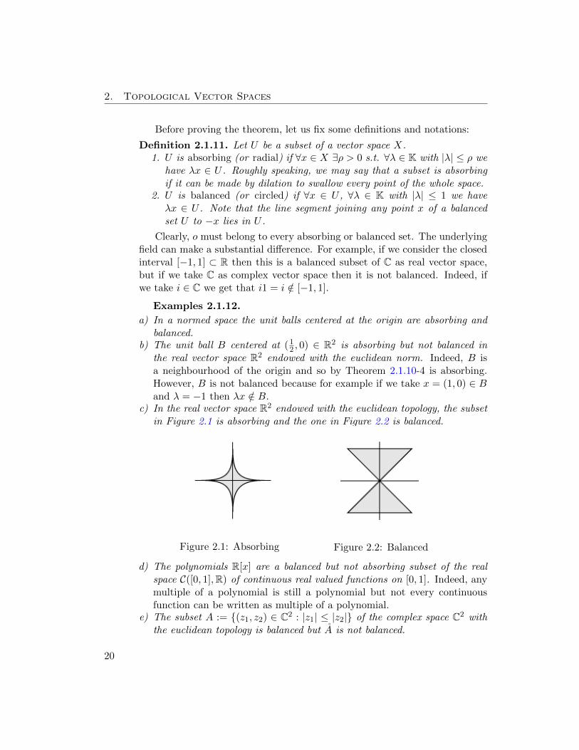
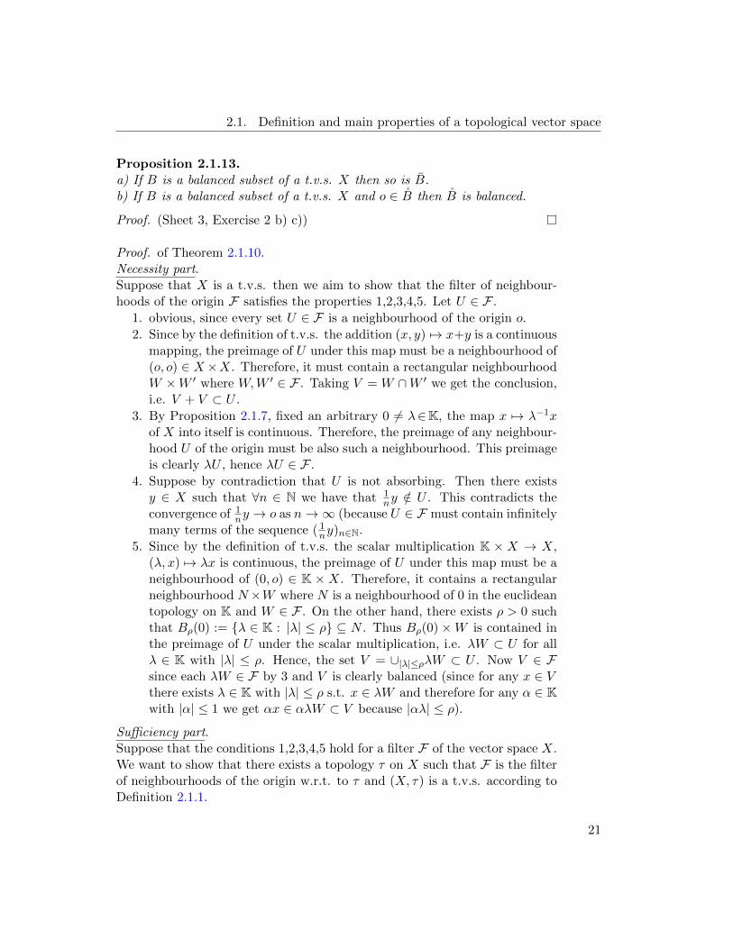
c) In the real vector space R2 endowed with the euclidean topology, the subsetin Figure 2.1 is absorbing and the one in Figure 2.2 is balanced.

Figure 2.1: Absorbing Figure 2.2: Balanced

d) The polynomials R[x] are a balanced but not absorbing subset of the realspace C([0, 1],R) of continuous real valued functions on [0, 1]. Indeed, anymultiple of a polynomial is still a polynomial but not every continuousfunction can be written as multiple of a polynomial.

e) The subset A := (z1, z2) ∈ C2 : |z1| ≤ |z2| of the complex space C2 withthe euclidean topology is balanced but A is not balanced.

20


Proposition 2.1.13.a) If B is a balanced subset of a t.v.s. X then so is B.b) If B is a balanced subset of a t.v.s. X and o ∈ B then B is balanced.

Proof. (Sheet 3, Exercise 2 b) c))

Proof. of Theorem 2.1.10.Necessity part.Suppose that X is a t.v.s. then we aim to show that the filter of neighbour-hoods of the origin F satisfies the properties 1,2,3,4,5. Let U ∈ F .

1. obvious, since every set U ∈ F is a neighbourhood of the origin o.

2. Since by the definition of t.v.s. the addition (x, y) 7→ x+y is a continuousmapping, the preimage of U under this map must be a neighbourhood of(o, o) ∈ X×X. Therefore, it must contain a rectangular neighbourhoodW ×W ′ where W,W ′ ∈ F . Taking V = W ∩W ′ we get the conclusion,i.e. V + V ⊂ U .

3. By Proposition 2.1.7, fixed an arbitrary 0 6= λ∈K, the map x 7→ λ−1xof X into itself is continuous. Therefore, the preimage of any neighbour-hood U of the origin must be also such a neighbourhood. This preimageis clearly λU , hence λU ∈ F .

4. Suppose by contradiction that U is not absorbing. Then there existsy ∈ X such that ∀n ∈ N we have that 1

ny /∈ U . This contradicts theconvergence of 1

ny → o as n→∞ (because U ∈ F must contain infinitelymany terms of the sequence ( 1

ny)n∈N.

5. Since by the definition of t.v.s. the scalar multiplication K × X → X,(λ, x) 7→ λx is continuous, the preimage of U under this map must be aneighbourhood of (0, o) ∈ K × X. Therefore, it contains a rectangularneighbourhood N×W where N is a neighbourhood of 0 in the euclideantopology on K and W ∈ F . On the other hand, there exists ρ > 0 suchthat Bρ(0) := λ ∈ K : |λ| ≤ ρ ⊆ N . Thus Bρ(0)×W is contained inthe preimage of U under the scalar multiplication, i.e. λW ⊂ U for allλ ∈ K with |λ| ≤ ρ. Hence, the set V = ∪|λ|≤ρλW ⊂ U . Now V ∈ Fsince each λW ∈ F by 3 and V is clearly balanced (since for any x ∈ Vthere exists λ ∈ K with |λ| ≤ ρ s.t. x ∈ λW and therefore for any α ∈ Kwith |α| ≤ 1 we get αx ∈ αλW ⊂ V because |αλ| ≤ ρ).

Sufficiency part.Suppose that the conditions 1,2,3,4,5 hold for a filter F of the vector space X.We want to show that there exists a topology τ on X such that F is the filterof neighbourhoods of the origin w.r.t. to τ and (X, τ) is a t.v.s. according toDefinition 2.1.1.

21


Let us define for any x ∈ X the filter F(x) := U + x : U ∈ F. It iseasy to see that F(x) fulfills the properties (N1) and (N2) of Theorem 1.1.9.In fact, we have:• By 1 we have that ∀U ∈ F , o ∈ U , then ∀U ∈ F , x = o+x ∈ U +x, i.e.∀A ∈ F(x), x ∈ A.• Let A ∈ F(x) then A = U + x for some U ∈ F . By 2, we have that

there exists V ∈ F s.t. V +V ⊂ U . Define B := V +x ∈ F(x) and takeany y ∈ B then we have V + y ⊂ V +B ⊂ V +V +x ⊂ U +x = A. ButV + y belongs to the filter F(y) and therefore so does A.

By Theorem 1.1.9, there exists a unique topology τ on X such that F(x) isthe filter of neighbourhoods of each point x ∈ X and so for which in particularF is the filter of neighbourhoods of the origin.

It remains to prove that the vector addition and the scalar multiplicationin X are continuous w.r.t. to τ .• The continuity of the addition easily follows from the property 2. Indeed,

let (x0, y0) ∈ X ×X and take a neighbourhood W of its image x0 + y0.Then W = U + x0 + y0 for some U ∈ F . By 2, there exists V ∈ F s.t.V + V ⊂ U and so (V + x0) + (V + y0) ⊂ W . This implies that thepreimage of W under the addition contains (V + x0) × (V + y0) whichis a neighbourhood of (x0, y0).• To prove the continuity of the scalar multiplication, let (λ0, x0) ∈ K×X

and take a neighbourhood U ′ of λ0x0. Then U ′ = U + λ0x0 for someU ∈ F . By 2 and 5, there exists W ∈ F s.t. W + W + W ⊂ U and Wis balanced. By 4, W is also absorbing so there exists ρ > 0 (w.l.o.g wecan take ρ ≤ 1) such that ∀λ ∈ K with |λ| ≤ ρ we have λx0 ∈W .

Suppose λ0 = 0 then λ0x0 = o and U ′ = U . Now

Im(Bρ(0)× (W + x0)) = λy + λx0 : λ ∈ Bρ(0), y ∈W.As λ ∈ Bρ(0) and W is absorbing, λx0 ∈ W . Also since |λ| ≤ ρ ≤ 1for all λ ∈ Bρ(0) and since W is balanced, we have λW ⊂ W . ThusIm(Bρ(0)×(W+x0)) ⊂W+W ⊂W+W+W ⊂ U and so the preimageof U under the scalar multiplication contains Bρ(0)× (W +x0) which isa neighbourhood of (0, x0).

Suppose λ0 6= 0 and take σ = minρ, |λ0|. Then Im((Bσ(0) +λ0)×(|λ0|−1W + x0))=λ|λ0|−1y+λx0 +λ0|λ0|−1y + λx0 : λ∈Bσ(0), y∈W.As λ ∈ Bσ(0), σ ≤ ρ and W is absorbing, λx0 ∈ W . Also since ∀λ ∈Bσ(0) the modulus of λ|λ0|−1 and λ0|λ0|−1 are both ≤ 1 and since Wis balanced, we have λ|λ0|−1W,λ0|λ0|−1W ⊂ W . Thus Im(Bσ(0) +λ0 × (|λ0|−1W + x0)) ⊂ W + W + W + λ0x0 ⊂ U + λ0x0 and so thepreimage of U + λ0x0 under the scalar multiplication contains Bσ(0) +λ0 × (|λ0|−1W + x0) which is a neighbourhood of (λ0, x0).

22


It easily follows from previous theorem that:

Corollary 2.1.14.

a) Every t.v.s. has always a base of closed neighbourhoods of the origin.b) Every t.v.s. has always a base of balanced absorbing neighbourhoods of the

origin. In particular, it has always a base of closed balanced absorbingneighbourhoods of the origin.

c) Proper subspaces of a t.v.s. are never absorbing. In particular, if M is anopen subspace of a t.v.s. X then M = X.


Let us show some further useful properties of the t.v.s.:

Proposition 2.1.15.

1. Every linear subspace of a t.v.s. endowed with the correspondent subspacetopology is itself a t.v.s..

2. The closure H of a linear subspace H of a t.v.s. X is again a linearsubspace of X.

3. Let X,Y be two t.v.s. and f : X → Y a linear map. f is continuous ifand only if f is continuous at the origin o.

Proof.

1. This clearly follows by the fact that the addition and the multiplicationrestricted to the subspace are just a composition of continuous maps(recall that inclusion is continuous in the subspace topology c.f. Defini-tion 1.1.17).

2. Let x0, y0 ∈ H and let us take any U ∈ F(o). By Theorem 2.1.10-2, there exists V ∈ F(o) s.t. V + V ⊂ U . Then, by definition ofclosure points, there exist x, y ∈ H s.t. x ∈ V + x0 and y ∈ V + y0.Therefore, we have that x + y ∈ H (since H is a linear subspace) andx+y ∈ (V +x0)+(V +y0) ⊂ U+x0 +y0. Hence, x0 +y0 ∈ H. Similarly,one can prove that if x0 ∈ H, λx0 ∈ H for any λ ∈ K.

3. Assume that f is continuous at o ∈ X and fix any x 6= o in X. Let U bean arbitrary neighbourhood of f(x) ∈ Y . By Corollary 2.1.9, we knowthat U = f(x) + V where V is a neighbourhood of o ∈ Y . Since f islinear we have that:

f−1(U) = f−1(f(x) + V ) ⊃ x+ f−1(V ).

By the continuity at the origin of X, we know that f−1(V ) is a neigh-bourhood of o ∈ X and so x+ f−1(V ) is a neighbourhood of x ∈ X.

23


2.2 Hausdorff topological vector spaces

For convenience let us recall here the definition of Hausdorff space.

Definition 2.2.1. A topological space X is said to be Hausdorff or (T2) ifany two distinct points of X have neighbourhoods without common points; orequivalently if two distinct points always lie in disjoint open sets.

Note that in a Hausdorff space, any set consisting of a single point isclosed but there are topological spaces with the same property which are notHausdorff and we will see in this section that such spaces are not t.v.s..

Definition 2.2.2. A topological space X is said to be (T1) if, given twodistinct points of X, each lies in a neighborhood which does not contain theother point; or equivalently if, for any two distinct points, each of them lies inan open subset which does not contain the other point.

It is easy to see that in a topological space which is (T1) all singletons areclosed (Sheet 4, Exercise 2).

From the definition it is clear that (T2) implies (T1) but in general theinverse does not hold (c.f. Examples 1.1.40-4 for an example of topologicalspace which is T1 but not T2). However, the following results shows that at.v.s is Hausdorff if and only if it is (T1).

Proposition 2.2.3. A t.v.s. X is Hausdorff iff

∀ o 6= x ∈ X, ∃U ∈ F(o) s.t. x /∈ U. (2.1)

Proof.(⇒) Let (X, τ) be Hausdorff. Then there exist U ∈ F(o) and V ∈ F(x)

s.t. U ∩ V = ∅. This means in particular that x /∈ U .(⇐) Assume that (2.1) holds and let x, y ∈ X with x 6= y, i.e. x− y 6= o.

Then there exists U ∈ F(o) s.t. x− y /∈ U . By (2) and (5) of Theorem 2.1.10,there exists V ∈ F(o) balanced and s.t. V + V ⊂ U . Since V is balancedV = −V then we have V − V ⊂ U . Suppose now that (V + x) ∩ (V + y) 6= ∅,then there exists z ∈ (V + x) ∩ (V + y), i.e. z = v + x = w + y for somev, w ∈ V . Then x − y = w − v ∈ V − V ⊂ U and so x − y ∈ U which is acontradiction. Hence, (V + x) ∩ (V + y) = ∅ and by Corollary 2.1.9 we knowthat V + x ∈ F(x) and V + y ∈ F(y). Hence, X is (T2).

Note that since the topology of a t.v.s. is translation invariant then theprevious proposition guarantees that a t.v.s is Hausdorff iff it is (T1). As amatter of fact, we have the following result:

24

2.3. Quotient topological vector spaces

Corollary 2.2.4. For a t.v.s. X the following are equivalent:a) X is Hausdorff.b) the intersection of all neighbourhoods of the origin o is just o.c) 0 is closed.

Note that in a t.v.s. 0 is closed is equivalent to say that all singletonsare closed (and so that the space is (T1)).

Proof.a)⇒ b) Let X be a Hausdorff t.v.s. space. Clearly, o ⊆ ∩U∈F(o)U . Nowif b) does not hold, then there exists x ∈ ∩U∈F(o)U with x 6= o. But by theprevious theorem we know that (2.1) holds and so there exists V ∈ F(o) s.t.x /∈ V and so x /∈ ∩U∈F(o)U which is a contradiction.

b)⇒ c) Assume that ∩U∈F(o)U = o. If x ∈ o then ∀Vx ∈ F(x) we haveVx ∩ o 6= ∅, i.e. o ∈ Vx. By Corollary 2.1.9 we know that each Vx = U + xwith U ∈ F(o). Then o = u + x for some u ∈ U and so x = −u ∈ −U . Thismeans that x ∈ ∩U∈F(o)(−U). Since every dilation is an homeomorphism and

b) holds, we have that x ∈ ∩U∈F(o)U = 0. Hence, x = 0 and so o = o,i.e. o is closed.

c)⇒ a) Assume that X is not Hausdorff. Then by the previous proposition(2.1) does not hold, i.e. there exists x 6= o s.t. x ∈ U for all U ∈ F(o). Thismeans that x ∈ ∩U∈F(o)U ⊆ ∩U∈F(o)closedU = o By c), o = o and sox = 0 which is a contradiction.

Example 2.2.5. Every vector space with an infinite number of elements en-dowed with the cofinite topology is not a tvs. It is clear that in such topologicalspace all singletons are closed (i.e. it is T1). Therefore, if it was a t.v.s. thenby the previous results it should be a Hausdorff space which is not true asshowed in Example 1.1.40.

2.3 Quotient topological vector spaces

Quotient topology

Let X be a topological space and ∼ be any equivalence relation on X. Thenthe quotient set X/∼ is defined to be the set of all equivalence classes w.r.t.to ∼. The map φ : X → X/∼ which assigns to each x ∈ X its equivalenceclass φ(x) w.r.t. ∼ is called the canonical map or quotient map. Note that φ issurjective. We may define a topology on X/ ∼ by setting that: a subset U ofX/∼ is open iff the preimage φ−1(U) is open in X. This is called the quotienttopology on X/ ∼. Then it is easy to verify (Sheet 4, Exercise 2) that:

25


• the quotient map φ is continuous.• the quotient topology on X/∼ is the finest topology on X/∼ s.t. φ is

continuous.Note that the quotient map φ is not necessarily open or closed.

Example 2.3.1. Consider R with the standard topology given by the modulusand define the following equivalence relation on R:

x ∼ y ⇔ (x = y ∨ x, y ⊂ Z).

Let R/∼ be the quotient set w.r.t ∼ and φ : R → R/∼ the correspondentquotient map. Let us consider the quotient topology on R/∼. Then φ is notan open map. In fact, if U is an open proper subset of R containing an integer,then φ−1(φ(U)) = U ∪ Z which is not open in R with the standard topology.Hence, φ(U) is not open in R/∼ with the quotient topology.

For an example of quotient map which is not closed see Example 2.3.3 inthe following.

Quotient vector space

Let X be a vector space and M a linear subspace of X. For two arbitraryelements x, y ∈ X, we define x ∼M y iff x − y ∈ M . It is easy to seethat ∼M is an equivalence relation: it is reflexive, since x − x = 0 ∈ M(every linear subspace contains the origin); it is symmetric, since x − y ∈ Mimplies −(x − y) = y − x ∈ M (if a linear subspace contains an element, itcontains its inverse); it is transitive, since x − y ∈ M , y − z ∈ M impliesx− z = (x− y) + (y− z) ∈M (when a linear subspace contains two vectors, italso contains their sum). Then X/M is defined to be the quotient set X/∼M ,i.e. the set of all equivalence classes for the relation ∼M described above. Thecanonical (or quotient) map φ : X → X/M which assigns to each x ∈ X itsequivalence class φ(x) w.r.t. the relation ∼M is clearly surjective. Using thefact that M is a linear subspace of X, it is easy to check that:

1. if x ∼M y, then ∀λ ∈ K we have λx ∼M λy.2. if x ∼M y, then ∀ z ∈ X we have x+ z ∼M y + z.

These two properties guarantee that the following operations are well-definedon X/M :• vector addition: ∀φ(x), φ(y) ∈ X/M , φ(x) + φ(y) := φ(x+ y)• scalar multiplication: ∀λ ∈ K, ∀φ(x) ∈ X/M , λφ(x) := φ(λx)

X/M with the two operations defined above is a vector space and thereforeit is often called quotient vector space. Then the quotient map φ is clearlylinear.

26

2.3. Quotient topological vector spaces

Quotient topological vector space

Let X be now a t.v.s. and M a linear subspace of X. Consider the quotientvector space X/M and the quotient map φ : X → X/M defined in Section 2.3.Since X is a t.v.s, it is in particular a topological space, so we can consideron X/M the quotient topology defined in Section 2.3. We already know thatin this topological setting φ is continuous but actually the structure of t.v.s.on X guarantees also that it is open.

Proposition 2.3.2. For a linear subspace M of a t.v.s.X, the quotient map-ping φ : X → X/M is open (i.e. carries open sets in X to open sets in X/M)when X/M is endowed with the quotient topology.

Proof. Let V open in X. Then we have

φ−1(φ(V )) = V +M = ∪m∈M (V +m)

Since X is a t.v.s, its topology is translation invariant and so V + m is openfor any m ∈ M . Hence, φ−1(φ(V )) is open in X as union of open sets. Bydefinition, this means that φ(V ) is open in X/M endowed with the quotienttopology.

It is then clear that φ carries neighborhoods of a point in X into neighbor-hoods of a point in X/M and viceversa. Hence, the neighborhoods of theorigin in X/M are direct images under φ of the neighborhoods of the originin X. In conclusion, when X is a t.v.s and M is a subspace of X, we canrewrite the definition of quotient topology on X/M in terms of neighborhoodsas follows: the filter of neighborhoods of the origin of X/M is exactly the im-age under φ of the filter of neighborhoods of the origin in X.

It is not true, in general (not even when X is a t.v.s. and M is a subspaceof X), that the quotient map is closed.

Example 2.3.3.Consider R2 with the euclidean topology and the hyperbola H := (x, y) ∈ R2 :xy = 1. If M is one of the coordinate axes, then R2/M can be identifiedwith the other coordinate axis and the quotient map φ with the orthogonalprojection on it. All these identifications are also valid for the topologies. Thehyperbola H is closed in R2 but its image under φ is the complement of theorigin on a straight line which is open.

27


Corollary 2.3.4. For a linear subspace M of a t.v.s. X, the quotient spaceX/M endowed with the quotient topology is a t.v.s..

Proof.For convenience, we denote here by A the vector addition in X/M and just by+ the vector addition in X. Let W be a neighbourhood of the origin o in X/M .We aim to prove that A−1(W ) is a neighbourhood of (o, o) in X/M ×X/M .

The continuity of the quotient map φ : X → X/M implies that φ−1(W )is a neighbourhood of the origin in X. Then, by Theorem 2.1.10-2 (we canapply the theorem because X is a t.v.s.), there exists V neighbourhood ofthe origin in X s.t. V + V ⊆ φ−1(W ). Hence, by the linearity of φ, we getA(φ(V ) × φ(V )) = φ(V + V ) ⊆ W , i.e. φ(V ) × φ(V ) ⊆ A−1(W ). Since φ isalso open, φ(V ) is a neighbourhood of the origin o in X/M and so A−1(W ) isa neighbourhood of (o, o) in X/M ×X/M .

A similar argument gives the continuity of the scalar multiplication.

Proposition 2.3.5. Let X be a t.v.s. and M a linear subspace of X. ConsiderX/M endowed with the quotient topology. Then the two following propertiesare equivalent:a) M is closedb) X/M is Hausdorff

Proof.In view of Corollary 2.2.4, (b) is equivalent to say that the complement of theorigin in X/M is open w.r.t. the quotient topology. But the complement ofthe origin in X/M is exactly the image under φ of the complement of M in X.Since φ is an open continuous map, the image under φ of the complement of Min X is open in X/M iff the complement of M in X is open, i.e.(a) holds.

Corollary 2.3.6. If X is a t.v.s., then X/o endowed with the quotienttopology is a Hausdorff t.v.s.. X/o is said to be the Hausdorff t.v.s. asso-ciated with the t.v.s. X. When a t.v.s. X is Hausdorff, X and X/o aretopologically isomorphic.

Proof.Since X is a t.v.s. and o is a linear subspace of X, o is a closed linearsubspace of X. Then, by Corollary 2.3.4 and Proposition 2.3.5, X/o is aHausdorff t.v.s.. If in addition X is Hausdorff, then Corollary 2.2.4 guaran-tees that o = o in X. Therefore, the quotient map φ : X → X/o isalso injective because in this case Ker(φ) = o. Hence, φ is a topologicalisomorphism (i.e. bijective, continuous, open, linear) between X and X/owhich is indeed X/o.

28

2.4. Continuous linear mappings between t.v.s.

2.4 Continuous linear mappings between t.v.s.

Let X and Y be two vector spaces over K and f : X → Y a linear map. Wedefine the image of f , and denote it by Im(f), as the subset of Y :

Im(f) := y ∈ Y : ∃x ∈ X s.t. y = f(x).

We define the kernel of f , and denote it by Ker(f), as the subset of X:

Ker(f) := x ∈ X : f(x) = 0.

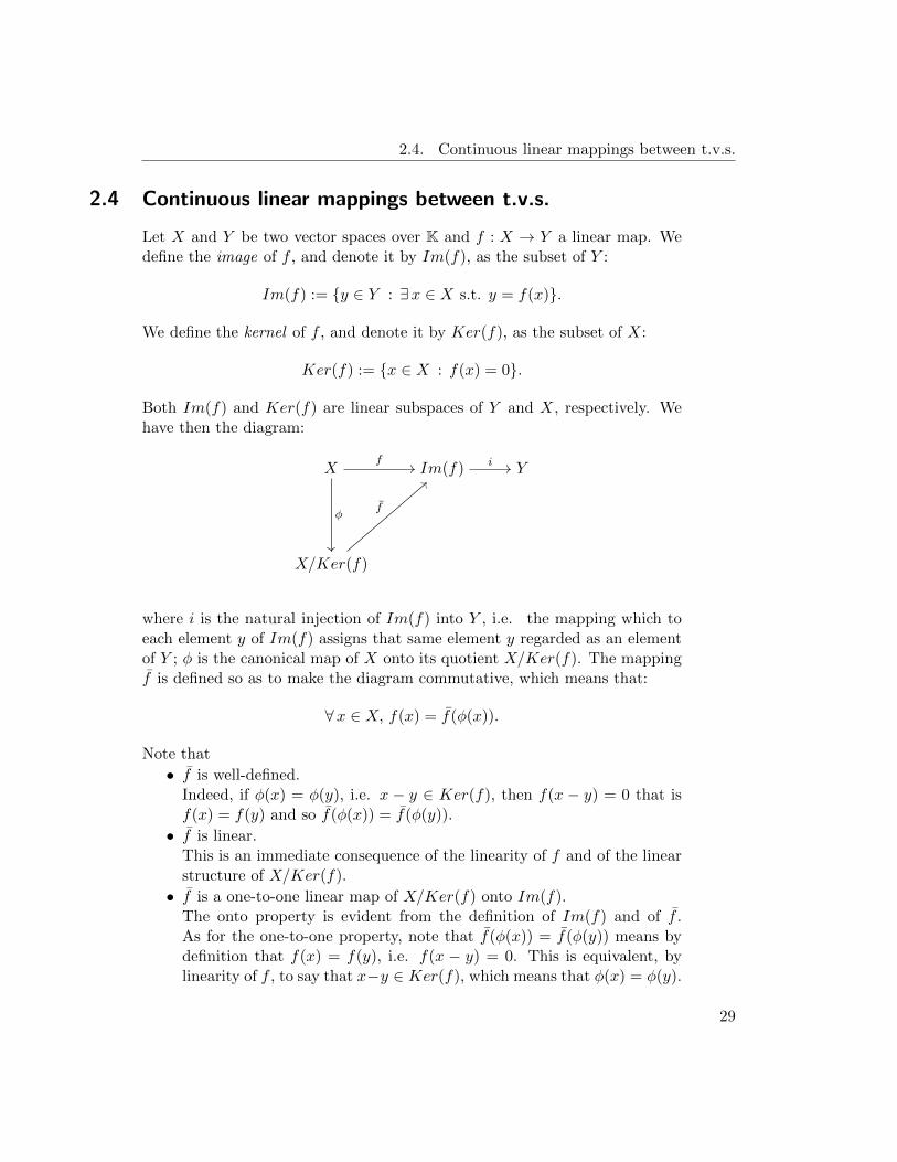
Both Im(f) and Ker(f) are linear subspaces of Y and X, respectively. Wehave then the diagram:

X Im(f) Y

X/Ker(f)

φ

f i

f

where i is the natural injection of Im(f) into Y , i.e. the mapping which toeach element y of Im(f) assigns that same element y regarded as an elementof Y ; φ is the canonical map of X onto its quotient X/Ker(f). The mappingf is defined so as to make the diagram commutative, which means that:

∀x ∈ X, f(x) = f(φ(x)).

Note that

• f is well-defined.Indeed, if φ(x) = φ(y), i.e. x − y ∈ Ker(f), then f(x − y) = 0 that isf(x) = f(y) and so f(φ(x)) = f(φ(y)).

• f is linear.This is an immediate consequence of the linearity of f and of the linearstructure of X/Ker(f).

• f is a one-to-one linear map of X/Ker(f) onto Im(f).The onto property is evident from the definition of Im(f) and of f .As for the one-to-one property, note that f(φ(x)) = f(φ(y)) means bydefinition that f(x) = f(y), i.e. f(x − y) = 0. This is equivalent, bylinearity of f , to say that x−y ∈ Ker(f), which means that φ(x) = φ(y).

29


The set of all linear maps (continuous or not) of a vector space X into anothervector space Y is denoted by L(X;Y ). Note that L(X;Y ) is a vector spacefor the natural addition and multiplication by scalars of functions. Recall thatwhen Y = K, the space L(X;Y ) is denoted by X∗ and it is called the algebraicdual of X (see Definition 1.2.4).

Let us not turn to consider linear mapping between two t.v.s. X and Y .Since they posses a topological structure, it is natural to study in this settingcontinuous linear mappings.

Proposition 2.4.1. Let f : X → Y a linear map between two t.v.s. X and Y .If Y is Hausdorff and f is continuous, then Ker(f) is closed in X.

Proof.Clearly, Ker(f) = f−1(o). Since Y is a Hausdorff t.v.s., o is closed in Yand so, by the continuity of f , Ker(f) is also closed in Y .

Note that Ker(f) might be closed in X also when Y is not Hausdorff. Forinstance, when f ≡ 0 or when f is injective and X is Hausdorff.

Proposition 2.4.2. Let f : X → Y a linear map between two t.v.s. X and Y .The map f is continuous if and only if the map f is continuous.

Proof.Suppose f continuous and let U be an open subset in Im(f). Then f−1(U)is open in X. By definition of f , we have f−1(U) = φ(f−1(U)). Since thequotient map φ : X → X/Ker(f) is open, φ(f−1(U)) is open in X/Ker(f).Hence, f−1(U) is open in X/Ker(f) and so the map f is continuous. Vicev-ersa, suppose that f is continuous. Since f = f φ and φ is continuous, f isalso continuous as composition of continuous maps.

In general, the inverse of f , which is well defined on Im(f) since f is in-jective, is not continuous. In other words, f is not necessarily bi-continuous.

The set of all continuous linear maps of a t.v.s. X into another t.v.s. Y isdenoted by L(X;Y ) and it is a vector subspace of L(X;Y ). When Y = K, thespace L(X;Y ) is usually denoted by X ′ which is called the topological dual ofX, in order to underline the difference with X∗ the algebraic dual of X. X ′

is a vector subspace of X∗ and is exactly the vector space of all continuouslinear functionals, or continuous linear forms, on X. The vector spaces X ′ andL(X;Y ) will play an important role in the forthcoming and will be equippedwith various topologies.

30

2.5. Completeness for t.v.s.

2.5 Completeness for t.v.s.

This section aims to treat completeness for most general types of topologicalvector spaces, beyond the traditional metric framework. As well as in the caseof metric spaces, we need to introduce the definition of a Cauchy sequence ina t.v.s..

Definition 2.5.1. A sequence S := xnn∈N of points in a t.v.s. X is said tobe a Cauchy sequence if

∀U ∈ F(o) inX, ∃N ∈ N : xm − xn ∈ U, ∀m,n ≥ N. (2.2)

This definition agrees with the usual one if the topology of X is definedby a translation-invariant metric d. Indeed, in this case, a basis of neigh-bourhoods of the origin is given by all the open balls centered at the origin.Therefore, xnn∈N is a Cauchy sequence in such (X, d) iff ∀ ε > 0, ∃N ∈ N :xm − xn ∈ Bε(o), ∀m,n ≥ N , i.e. d(xm, xn) = d(xm − xn, o) < ε.

By using the subsequences Sm := xn ∈ S : n ≥ m of S, we can easilyrewrite (2.2) in the following way

∀U ∈ F(o) inX, ∃N ∈ N : SN − SN ⊂ U.

As we have already observed in Chapter 1, the collection B := Sm : m ∈ Nis a basis of the filter FS associated with the sequence S. This immediatelysuggests what the definition of a Cauchy filter should be:

Definition 2.5.2. A filter F on a subset A of a t.v.s. X is said to be a Cauchyfilter if

∀U ∈ F(o) inX, ∃M ⊂ A : M ∈ F and M −M ⊂ U.

In order to better illustrate this definition, let us come back to our refer-ence example of a t.v.s. X whose topology is defined by a translation-invariantmetric d. For any subset M of (X, d), recall that the diameter of M is definedas diam(M) := supx,y∈M d(x, y). Now if F is a Cauchy filter on X then, bydefinition, for any ε > 0 there exists M ∈ F s.t. M −M ⊂ Bε(o) and thissimply means that diam(M) ≤ ε. Therefore, Definition 2.5.2 can be rephrasedin this case as follows: a filter F on a subset A of such a metric t.v.s. X is aCauchy filter if it contains subsets of A of arbitrarily small diameter.

Going back to the general case, the following statement clearly holds.

Proposition 2.5.3. The filter associated with a Cauchy sequence in a t.v.s.X is a Cauchy filter.

31


Proposition 2.5.4.Let X be a t.v.s.. Then the following properties hold:

a) The filter of neighborhoods of a point x ∈ X is a Cauchy filter on X.

b) A filter finer than a Cauchy filter is a Cauchy filter.

c) Every converging filter is a Cauchy filter.

Proof.

a) Let F(x) be the filter of neighborhoods of a point x ∈ X and let U ∈ F(o).By Theorem 2.1.10, there exists V ∈ F(o) such that V − V ⊂ U andso such that (V + x) − (V + x) ⊂ U . Since X is a t.v.s., we know thatF(x) = F(o) + x and so M := V + x ∈ F(x). Hence, we have proved thatfor any U ∈ F(o) there exists M ∈ F(x) s.t. M −M ⊂ U , i.e. F(x) is aCauchy filter.

b) Let F and F ′ be two filters of subsets of X such that F is a Cauchyfilter and F ⊆ F ′. Since F is a Cauchy filter, by Definition 2.5.2, for anyU ∈ F(o) there exists M ∈ F s.t. M −M ⊂ U . But F ′ is finer than F , soM belongs also to F ′. Hence, F ′ is obviously a Cauchy filter.

c) If a filter F converges to a point x ∈ X then F(x) ⊆ F (see Defini-tion 1.1.27). By a), F(x) is a Cauchy filter and so b) implies that F itselfis a Cauchy filter.

The converse of c) is in general false, in other words not every Cauchyfilter converges.

Definition 2.5.5. A subset A of a t.v.s. X is said to be complete if everyCauchy filter on A converges to a point x of A.

It is important to distinguish between completeness and sequentially com-pleteness.

Definition 2.5.6. A subset A of a t.v.s. X is said to be sequentially completeif any Cauchy sequence in A converges to a point in A.

It is easy to see that complete always implies sequentially complete. Theconverse is in general false (see Example 2.5.9). We will encounter an impor-tant class of t.v.s., the so-called metrizable spaces, for which the two notionscoincide.

Proposition 2.5.7. If a subset A of a t.v.s. X is complete then A is sequen-tially complete.

32


Proof.Let S := xnn∈N a Cauchy sequence of points in A. Then Proposition 2.5.3guarantees that the filter FS associated to S is a Cauchy filter in A. By thecompleteness of A we get that there exists x ∈ A such that FS converges to x.This is equivalent to say that the sequence S is convergent to x ∈ A (seeProposition 1.1.29). Hence, A is sequentially complete.

Before showing an example of a subset of a t.v.s. which is sequentiallycomplete but not complete, let us introduce two useful properties about com-pleteness in t.v.s..

Proposition 2.5.8.

a) In a Hausdorff t.v.s. X, any complete subset is closed.

b) In a complete t.v.s. X, any closed subset is complete.

Example 2.5.9.Let X := Rd where d > ℵ0 endowed with the product topology given by

considering each copy of R equipped with the usual topology given by the mod-ulus. For convenience we write X =

∏i∈J R with |J | = d > ℵ0. Note that X

is a Hausdorff t.v.s. as it is product of Hausdorff t.v.s.. Denote by H the sub-set of X consisting of all vectors x = (xi)i∈J in X with only countably manynon-zero coordinates xi. Claim: H is sequentially complete but not complete.

Proof. of Claim. Let us first make some observations on H.

• H is strictly contained in X.Indeed, any vector y ∈ X with all non-zero coordinates does not belongto H because d > ℵ0.

• H is dense in X.In fact, let x = (xi)i∈J ∈ X and U a neighbourhood of x in X. Then,by definition of product topology on X, there exist

∏i∈J Ui ⊆ U s.t.

Ui ⊆ R neighbourhood of xi in R for all i ∈ J and Ui 6= R for all i ∈ Iwhere I ⊂ J with |I| < ∞. Take y := (yi)i∈J s.t. yi ∈ Ui for all i ∈ Jwith yi 6= 0 for all i ∈ I and yi = 0 otherwise. Then clearly y ∈ Ubut also y ∈ H because it has only finitely many non-zero coordinates.

Hence, U ∩H 6= ∅ and so H = X.

Now suppose that H is complete, then by Proposition 2.5.8-a) we have thatH is closed. Therefore, by the density of H in X, it follows that H = H = Xwhich contradicts the first of the property above. Hence, H is not complete.

In the end, let us show that H is sequentially complete. Let (xn)n∈N a

Cauchy sequence of vectors xn = (x(i)n )i∈J in H. Then for each i ∈ J we have

that the sequence of the i − th coordinates (x(i)n )n∈N is a Cauchy sequence

33


in R. By the completeness (i.e. the sequentially completeness) of R we have

that for each i ∈ J , the sequence (x(i)n )n∈N converges to a point x(i) ∈ R. Set

x := (x(i))i∈J . Then:

• x ∈ H, because for each n ∈ N only countably many x(i)n 6= 0 and so

only countably many x(i) 6= 0.

• the sequence (xn)n∈N converges to x in H. In fact, for any U neighbour-hood of x in X there exist

∏i∈J Ui ⊆ U s.t. Ui ∈ R neighbourhood of

xi in R for all i ∈ J and Ui 6= R for all i ∈ I where I ⊂ J with |I| <∞.

Since for each i ∈ J , the sequence (x(i)n )n∈N converges to x(i) in R, we

get that for each i ∈ J there exists Ni ∈ N s.t. x(i)n ∈ Ui for all n ≥ Ni.

Take N := maxi∈I Ni (the max exists because I is finite). Then for each

i ∈ J we get x(i)n ∈ Ui for all n ≥ N , i.e. xn ∈ U for all n ≥ N which

proves the convergence of (xn)n∈N to x.

Hence, we have showed that every Cauchy sequence in H is convergent.

In order to prove Proposition 2.5.8, we need two small lemmas regardingconvergence of filters in a topological space.

Lemma 2.5.10. Let F be a filter of a topological Hausdorff space X. If Fconverges to x ∈ X and also to y ∈ X, then x = y.

Proof.Suppose that x 6= y. Then, since X is Hausdorff, there exists V ∈ F(x) andW ∈ F(y) such that V ∩W = ∅. On the other hand, we know by assumptionthat F → x and F → y that is F(x) ⊆ F and F(y) ⊆ F (see Definition 1.1.27).Hence, V,W ∈ F . Since filters are closed under finite intersections, we getthat V ∩W ∈ F and so ∅ ∈ F which contradicts the fact that F is a filter.

Lemma 2.5.11. Let A be a subset of a topological space X. Then x ∈ A ifand only if there exists a filter F of subsets of X such that A ∈ F and Fconverges to x.

Proof.Let x ∈ A, i.e. for any U ∈ F(x) in X we have U ∩ A 6= ∅. Set F :=

F ⊆ X|U ∩A ⊆ F for some U ∈ F(x). It is easy to see that F is a filter ofsubsets of X. Therefore, for any U ∈ F(x), U ∩A ∈ F and U ∩A ⊆ U implythat U ∈ F , i.e. F(x) ⊆ F . Hence, F → x.

Viceversa, suppose that F is a filter of X s.t. A ∈ F and F converges tox. Let U ∈ F(x). Then U ∈ F since F(x) ⊆ F by definition of convergence.Since also A ∈ F by assumption, we get U ∩A ∈ F and so U ∩A 6= ∅.

34


Proof. of Proposition 2.5.8a) Let A be a complete subset of a Hausdorff t.v.s. X and let x ∈ A. By

Lemma 2.5.11, x ∈ A implies that there exists a filter F of subsets of Xs.t. A ∈ F and F converges to x. Therefore, by Proposition 2.5.4-c), F isa Cauchy filter. Consider now FA := U ∈ F : U ⊆ A ⊂ F . It is easy tosee that FA is a Cauchy filter on A and so the completeness of A ensuresthat FA converges to a point y ∈ A. Hence, any nbhood V of y in Abelongs to FA and so to F . By definition of subset topology, this meansthat for any nbhood U of y in X we have U ∩A ∈ F and so U ∈ F (sinceF is a filter). Then F converges to y. Since X is Hausdorff, Lemma 2.5.10establishes the uniqueness of the limit point of F , i.e. x = y and so A = A.

b) Let A be a closed subset of a complete t.v.s. X and let FA be any Cauchyfilter on A. Take the filter F := F ⊆ X|B ⊆ F for some B ∈ FA. It isclear that F contains A and is finer than the Cauchy filter FA. Therefore,by Proposition 2.5.4-b), F is also a Cauchy filter. Then the completenessof the t.v.s. X gives that F converges to a point x ∈ X, i.e. F(x) ⊆ F .By Lemma 2.5.11, this implies that actually x ∈ A and, since A is closed,that x ∈ A. Now any neighbourhood of x ∈ A in the subset topology isof the form U ∩ A with U ∈ F(x). Since F(x) ⊆ F and A ∈ F , we haveU ∩ A ∈ F . Therefore, there exists B ∈ FA s.t. B ⊆ U ∩ A ⊂ A and soU ∩A ∈ FA. Hence, FA converges x ∈ A, i.e. A is complete.

When a t.v.s. is not complete, it makes sense to ask if it is possible toembed it in a complete one. We are going to describe an abstract procedurethat allows to always associate to an arbitrary Hausdorff t.v.s. X a completeHausdorff t.v.s. X called the completion of X. Before doing that, we needto introduce uniformly continuous functions between t.v.s. and state some oftheir fundamental properties.

Definition 2.5.12. Let X and Y be two t.v.s. and let A be a subset of X. Amapping f : A → Y is said to be uniformly continuous if for every neighbor-hood V of the origin in Y , there exists a neighborhood U of the origin in Xsuch that for all pairs of elements x1, x2 ∈ A

x1 − x2 ∈ U ⇒ f(x1)− f(x2) ∈ V.

Proposition 2.5.13. Let X and Y be two t.v.s. and let A be a subset of X.a) If f : A→ Y is uniformly continuous, then the image under f of a Cauchy

filter on A is a Cauchy filter on Y .b) If A is a linear subspace of X, then every continuous linear map from A

to Y is uniformly continuous.


35


Theorem 2.5.14.Let X and Y be two Hausdorff t.v.s., A a dense subset of X, and f : A→ Ya uniformly continuous mapping. If Y is complete the the following hold.

a) There exists a unique continuous mapping f : X → Y which extends f ,i.e. such that for all x ∈ A we have f(x) = f(x).

b) f is uniformly continuous.

c) If we additionally assume that f is linear and A is a linear subspace of X,then f is linear.


Let us now state and prove the theorem on completion of a t.v.s..

Theorem 2.5.15.Let X be a Haudorff t.v.s.. Then there exists a complete Hausdorff t.v.s. Xand a mapping i : X → X with the following properties:

a) The mapping i is a topological monomorphism.

b) The image of X under i is dense in X.

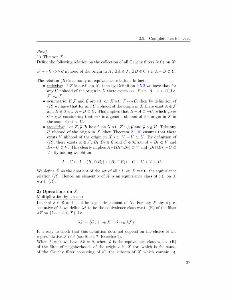
c) For every complete Hausdorff t.v.s. Y and for every continuous linear mapf : X → Y , there is a continuous linear map f : X → Y such that thefollowing diagram is commutative:

X Y

X

i

f

f

Furthermore:

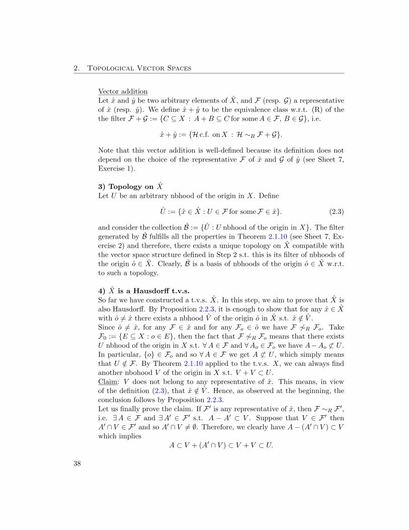
I) Any other pair (X1, i1), consisting of a complete Hausdorff t.v.s. X1

and of a mapping i1 : X → X1 such that properties (a) and (b) holdsubstituting X with X1 and i with i1, is topologically isomorphic to (X, i).This means that there is a topological isomorphism j of X onto X1 suchthat the following diagram is commutative:

X X1

X

i

i1

j

II) Given Y and f as in property (c), the continuous linear map f is unique.

36


Proof.1) The set XDefine the following relation on the collection of all Cauchy filters (c.f.) on X:

F ∼R G ⇔ ∀U nbhood of the origin in X, ∃A ∈ F , ∃B ∈ G s.t. A−B ⊂ U.

The relation (R) is actually an equivalence relation. In fact:• reflexive: If F is a c.f. on X, then by Definition 2.5.2 we have that for

any U nbhood of the origin in X there exists A ∈ F s.t. A−A ⊂ U , i.e.F ∼R F .• symmetric: If F and G are c.f. on X s.t. F ∼R G, then by definition of

(R) we have that for any U nbhood of the origin in X there exist A ∈ Fand B ∈ G s.t. A−B ⊂ U . This implies that B −A ⊂ −U , which givesG ∼R F considering that −U is a generic nbhood of the origin in X inthe same right as U .• transitive: Let F ,G,H be c.f. on X s.t. F ∼R G and G ∼R H. Take anyU nbhood of the origin in X, then Theorem 2.1.10 ensures that thereexists V nbhood of the origin in X s.t. V + V ⊂ U . By definition of(R), there exists A ∈ F , B1, B2 ∈ G and C ∈ H s.t. A − B1 ⊂ V andB2−C ⊂ V . This clearly implies A−(B1∩B2) ⊂ V and (B1∩B2)−C ⊂V . By adding we obtain

A− C ⊂ A− (B1 ∩B2) + (B1 ∩B2)− C ⊂ V + V ⊂ U.

We define X as the quotient of the set of all c.f. on X w.r.t. the equivalencerelation (R). Hence, an element x of X is an equivalence class of c.f. on Xw.r.t. (R).

2) Operations on XMultiplication by a scalar

Let 0 6= λ ∈ K and let x be a generic element of X. For any F any repre-sentative of x, we define λx to be the equivalence class w.r.t. (R) of the filterλF := λA : A ∈ F, i.e.

λx := G c.f. onX : G ∼R λF.

It is easy to check that this definition does not depend on the choice of therepresentative F of x (see Sheet 7, Exercise 1).When λ = 0, we have λx = o, where o is the equivalence class w.r.t. (R)of the filter of neighborhoods of the origin o in X (or, which is the same,of the Cauchy filter consisting of all the subsets of X which contain o).

37


Vector additionLet x and y be two arbitrary elements of X, and F (resp. G) a representativeof x (resp. y). We define x + y to be the equivalence class w.r.t. (R) of thethe filter F + G := C ⊆ X : A+B ⊆ C for someA ∈ F , B ∈ G, i.e.

x+ y := H c.f. onX : H ∼R F + G.

Note that this vector addition is well-defined because its definition does notdepend on the choice of the representative F of x and G of y (see Sheet 7,Exercise 1).

3) Topology on XLet U be an arbitrary nbhood of the origin in X. Define

U := x ∈ X : U ∈ F for someF ∈ x. (2.3)

and consider the collection B := U : U nbhood of the origin in X. The filtergenerated by B fulfills all the properties in Theorem 2.1.10 (see Sheet 7, Ex-ercise 2) and therefore, there exists a unique topology on X compatible withthe vector space structure defined in Step 2 s.t. this is its filter of nbhoods ofthe origin o ∈ X. Clearly, B is a basis of nbhoods of the origin o ∈ X w.r.t.to such a topology.

4) X is a Hausdorff t.v.s.So far we have constructed a t.v.s. X. In this step, we aim to prove that X isalso Hausdorff. By Proposition 2.2.3, it is enough to show that for any x ∈ Xwith o 6= x there exists a nbhood V of the origin o in X s.t. x /∈ V .Since o 6= x, for any F ∈ x and for any Fo ∈ o we have F 6∼R Fo. TakeF0 := E ⊆ X : o ∈ E, then the fact that F 6∼R Fo means that there existsU nbhood of the origin in X s.t. ∀A ∈ F and ∀Ao ∈ Fo we have A−Ao 6⊂ U .In particular, o ∈ Fo and so ∀A ∈ F we get A 6⊂ U , which simply meansthat U /∈ F . By Theorem 2.1.10 applied to the t.v.s. X, we can always findanother nbohood V of the origin in X s.t. V + V ⊂ U .Claim: V does not belong to any representative of x. This means, in viewof the definition (2.3), that x /∈ V . Hence, as observed at the beginning, theconclusion follows by Proposition 2.2.3.Let us finally prove the claim. If F ′ is any representative of x, then F ∼R F ′,i.e. ∃A ∈ F and ∃A′ ∈ F ′ s.t. A − A′ ⊂ V . Suppose that V ∈ F ′ thenA′ ∩ V ∈ F ′ and so A′ ∩ V 6= ∅. Therefore, we clearly have A− (A′ ∩ V ) ⊂ Vwhich implies

A ⊂ V + (A′ ∩ V ) ⊂ V + V ⊂ U.

38


Since A ∈ F , this proves that U ∈ F which is a contradiction. Then V /∈ F ′for all F ′ ∈ x that is exactly our claim.

5) Existence of i : X → XWe define the image of a point x ∈ X under the mapping i : X → X to bethe equivalence class w.r.t. (R) of the filter F(x) of neighborhoods of x in X,i.e.

∀x ∈ X, i(x) := F c.f. onX : F ∼R F(x).

Note that the following properties hold.

Lemma 2.5.16.

a) Two c.f. filters on X converging to the same point are equivalent w.r.t. (R)

b) If two c.f. filters F and F ′ on X are s.t. F ∼R F ′ and F ′ converges tox ∈ X then also F converges to x.


The previous lemma clearly proves that

i(x) ≡ F c.f. onX : F → x).

6) i is a topological monomorphism (i.e. (a) holds)i is injective

(see Sheet 7, Exercise 4).

i is a topological homomorphismFor the linearity of i see Sheet 7, Exercise 4. We aim to show here that i isboth open and continuous on X.

To prove that i is open, we need to show that for any nbhood U of theorigin in X the image i(U) is a nbhood of the origin in i(X) endowed withthe subset topology induced by the topology on X. Therefore, it suffices toshow that for any nbhood U of the origin in X there exists U1 nbhood of theorigin in X s.t.

U1 ∩ i(X) ⊆ i(U) (2.4)

where U1 is defined as in (2.3).

To show the continuity of i, we need to prove that for any nbhood Vof the origin in i(X) the preimage i−1(V ) is a nbhood of the origin in X.Now any nbhood of the origin in i(X) is of the form U1 ∩ i(X) for some U1

nbhood of the origin in X. Therefore, it is enough to show that for any U1

39


nbhood of the origin in X there exists another U nbhood of the origin in Xs.t. U ⊆ i−1(U1 ∩ i(X)) i.e.

i(U) ⊆ U1 ∩ i(X) (2.5)

In order to prove (2.4) and (2.5), we shall prove the following:

i(V ) ⊆ V ∩ i(X) ⊆ i(V ), ∀V nbhood of the origin in X. (2.6)

Indeed, if (2.6) holds then the first inclusion immediately shows (2.5) (for anyU1 nbhood of the origin in X take U := U1 and apply the first inclusion of(2.6) to V = U1). Moreover, (2.4) follows by combining the fact that for anynbhood U of the origin in X exists another nbhood U1 of the origin in X s.t.U1 = U1 ⊆ U (c.f. Sheet 3, Ex3-a)) together with the second inclusion of (2.6)(applied to U1).

It remains to prove that (2.6) holds. Let V be any nbhood of the originin X, then for any x ∈ V we clearly have that V is a nbhood of x, whichmeans that V belongs to a representative of i(x), i.e. i(x) ∈ V . Hence,i(V ) ⊆ V ∩ i(X). Now take y ∈ V ∩ i(X), i.e. y = i(x) for some x ∈ X s.t.i(x) ∈ V . Then, by definition (2.3), we have that V ∈ F for some F ∈ i(x)or in other words that V belongs to some filter F converging to x. Let Wbe another nbhood of the origin in X then W + x is a nbhood of x in X andso W + x ∈ F (since F → x). Hence, V ∩ (W + x) ∈ F which implies thatV ∩ (W + x) 6= ∅ i.e. x ∈ V . This means that y = i(x) ∈ i(V ) which provesV ∩ i(X) ⊆ i(V ).

7) i(X) = X (i.e. (b) holds)Let xo ∈ X and let N be any nbhood of xo in X. It suffices to consider theneighborhoods N of the form U + x0 where U is defined by (2.3) for some Unbhood of the origin in X. We aim to prove that (U + xo) ∩ i(X) 6= ∅.

By Theorem 2.1.10, we know that for any U nbhood of the origin in Xthere exists V nbhood of the origin in X s.t. V + V ⊂ U . Let Fo be arepresentative of x0, then Fo is a c.f. on X and so there exists Ao ∈ Fo s.t.Ao −Ao ⊂ V . Fix an element x ∈ Ao. Then we get:

(V + x)−Ao ⊂ V +Ao −Ao ⊂ V + V ⊂ U. (2.7)

Since V + x is a nbhood of x in X, V + x belongs to any Cauchy filter F con-verging to x and so V +x ∈ F for any F ∈ i(x). Then (V +x)−Ao ∈ F −Foand so (2.7) gives U ∈ F −Fo i.e. i(x)− xo ∈ U . Hence, we found that thereexists x ∈ X s.t. i(x) ∈ U + xo which gives the conclusion.

40


8) X is completeLet F be a Cauchy filter on X. We aim to prove that there exists an elementx ∈ X s.t. F → x.

Consider the filter

F ′ := G ⊂ X : M+U ⊂ G for some M ∈ F and U nbhood of the origin in X.

Note that F ′ ⊂ F and F ′ is also a Cauchy filter on X. In fact, since X is at.v.s., for any U nbhood of the origin in X there exists V0 balanced nbhood ofthe origin in X s.t. V0 + V0 + V0 ⊂ U . Take V := 1

3 V0 which is also a nbhood

of the origin in X, then

V + V − V ⊂ V0 + V0 + V0 ⊂ U.

Since F is a Cauchy filter, there exists M ∈ F s.t. M − M ⊂ V . Then

(M + V )− (M + V ) ⊂ V + V − V ⊂ U

Now let us consider the family of subsets of i(X) given by

F ′ := A ∩ i(X) : A ∈ F ′.

It is possible to prove that F ′ is a filter on i(X) and actually a Cauchy filter(see Sheet 7, Exercise 5). Moreover, since we proved that i is a topologicalisomorphism between X and i(X), we have that i−1(F ′) is a Cauchy filter onX. Take

x := F c.f. on X : F ∼R i−1(F ′).

Then F converges to x (see Sheet 7, Exercise 5).

9) Proof of the universal property (i.e. (c) and (II))We can now identify X with i(X) and so regard X as a dense linear subspaceof X. Since f : X → Y is continuous and linear by assumption, it is alsouniformly continuous by Proposition 2.5.13. Then applying Theorem 2.5.14with X replaced by X and A by X we get both the properties (c) and (II).

10) Uniqueness of X up to isomorphism (proof of (I))Since by assumption X1 is a complete Hausdorff t.v.s. and i1 : X → X1

is a topological monomorphism (in particular i1 is a continuous linear map-ping), we have by (c) that there exists a unique continuous linear map i1 s.t.i1(i(x)) = i1(x) for any x ∈ X. Let us define j := i1. On the other hand,let us define f : i1(X) → X by f(i1(x)) = i(x) for any x ∈ X. Since f is

41


clearly linear and continuous and i1(X) is a linear subspace of X, f is uni-formly continuous and so by Theorem 2.5.14 we get that there exists a uniquef : X1 → X continuous and linear s.t. f(i1(x)) = f(i1(x)) for any x ∈ X.Using the density of i(X) in X, the density of i1(X) in X1 and the continuityof the mappings involved, it is easy to check that

f(j(x)) = x ∀ x ∈ X

and thatj(f(x1)) = x1 ∀ , x1 ∈ X1.

This means that j and f are the inverse of each other and that both aretopological isomorphisms.

42

Chapter 3

Finite dimensional topological vector spaces

3.1 Finite dimensional Hausdorff t.v.s.

Let X be a vector space over the field K of real or complex numbers. We knowfrom linear algebra that the (algebraic) dimension of X, denoted by dim(X),is the cardinality of a basis of X. If dim(X) is finite, we say that X is finitedimensional otherwise X is infinite dimensional. In this section we are goingto focus on finite dimensional vector spaces.

Let e1, . . . , ed be a basis of X, i.e. dim(X) = d. Given any vector x ∈ Xthere exist unique x1, . . . , xd ∈ K s.t. x = x1e1 + · · ·xded. This can be preciselyexpressed by saying that the mapping

Kd → X(x1, . . . , xd) 7→ x1e1 + · · ·xded

is an algebraic isomorphism (i.e. linear and bijective) between X and Kd. Inother words: If X is a finite dimensional vector space then X is algebraicallyisomorphic to Kdim(X).

If now we give to X the t.v.s. structure and we consider K endowed withthe euclidean topology, then it is natural to ask if such an algebraic isomor-phism is by any chance a topological one, i.e. if it preserves the t.v.s. structure.The following theorem shows that if X is a finite dimensional Hausdorff t.v.s.then the answer is yes: X is topologically isomorphic to Kdim(X). It is worthto observe that usually in applications we deal always with Hausdorff t.v.s.,therefore it makes sense to mainly focus on them.

Theorem 3.1.1. Let X be a finite dimensional Hausdorff t.v.s. over K (whereK is endowed with the euclidean topology). Then:

a) X is topologically isomorphic to Kd, where d = dim(X).

43

3. Finite dimensional topological vector spaces

b) Every linear functional on X is continuous.

c) Every linear map of X into any t.v.s. Y is continuous.

Before proving the theorem let us recall some lemmas about the continuityof linear functionals on t.v.s..

Lemma 3.1.2.Let X be a t.v.s. over K and v ∈ X. Then the following mapping is continuous.

ϕv : K → Xξ 7→ ξv.

Proof. For any ξ ∈ K, we have ϕv(ξ) = M(ψv(ξ)), where ψv : K → K × Xgiven by ψ(ξ) := (ξ, v) is clearly continuous by definition of product topologyand M : K × X → X is the scalar multiplication in the t.v.s. X which iscontinuous by definition of t.v.s.. Hence, ϕv is continuous as composition ofcontinuous mappings.

Lemma 3.1.3. Let X be a t.v.s. over K and L a linear functional on X.Assume L(x) 6= 0 for some x ∈ X. Then the following are equivalent:

a) L is continuous.

b) The null space Ker(L) is closed in X

c) Ker(L) is not dense in X.

d) L is bounded in some neighbourhood of the origin in X.

Proof. (see Sheet 4, Exercise 4)

Proof. of Theorem 3.1.1Let e1, . . . , ed be a basis of X and let us consider the mapping

ϕ : Kd → X(x1, . . . , xd) 7→ x1e1 + · · ·xded.

As noted above, this is an algebraic isomorphism. Therefore, to conclude a)it remains to prove that ϕ is also a homeomorphism.

Step 1: ϕ is continuous.When d = 1, we simply have ϕ ≡ ϕe1 and so we are done by Lemma3.1.2. When d > 1, for any (x1, . . . , xd) ∈ Kd we can write: ϕ(x1, . . . , xd) =A(ϕe1(x1), . . . , ϕed(xd)) = A((ϕe1 × · · · × ϕed)(x1, . . . , xd)) where each ϕej isdefined as above and A : X ×X → X is the vector addition in the t.v.s. X.Hence, ϕ is continuous as composition of continuous mappings.

44

3.1. Finite dimensional Hausdorff t.v.s.

Step 2: ϕ is open and b) holds.We prove this step by induction on the dimension dim(X) of X.For dim(X) = 1, it is easy to see that ϕ is open, i.e. that the inverse of ϕ:

ϕ−1 : X → Kx = ξe1 7→ ξ

is continuous. Indeed, we have that

Ker(ϕ−1) = x ∈ X : ϕ−1(x) = 0 = ξe1 ∈ X : ξ = 0 = o,

which is closed in X, since X is Hausdorff. Hence, by Lemma 3.1.3, ϕ−1 iscontinuous. This implies that b) holds. In fact, if L is a non-identically zerofunctional on X (when L ≡ 0, there is nothing to prove), then there existsa o 6= x ∈ X s.t. L(x) 6= 0. W.l.o.g. we can assume L(x) = 1. Now forany x ∈ X, since dim(X) = 1, we have that x = ξx for some ξ ∈ K and soL(x) = ξL(x) = ξ. Hence, L ≡ ϕ−1 which we proved to be continuous.

Suppose now that both a) and b) hold for dim(X) ≤ d−1. Let us first showthat b) holds when dim(X) = d. Let L be a non-identically zero functionalon X (when L ≡ 0, there is nothing to prove), then there exists a o 6= x ∈ Xs.t. L(x) 6= 0. W.l.o.g. we can assume L(x) = 1. Note that for any x ∈ X theelement x − xL(x) ∈ Ker(L). Therefore, if we take the canonical mappingφ : X → X/Ker(L) then φ(x) = φ(xL(x)) = L(x)φ(x) for any x ∈ X.This means that X/Ker(L) = spanφ(x) i.e. dim(X/Ker(L)) = 1. Hence,dim(Ker(L)) = d− 1 and so by inductive assumption Ker(L) is topologicallyisomorphic to Kd−1. This implies that Ker(L) is a complete subspace of X.Then, by Proposition 2.5.8-a), Ker(L) is closed in X and so by Lemma 3.1.3we get L is continuous. By induction, we can cocnlude that b) holds for anydimension d ∈ N.

This immediately implies that a) holds for any dimension d ∈ N. In fact,we just need to show that for any dimension d ∈ N the mapping

ϕ−1 : X → Kd

x =∑d

j=1 xjej 7→ (x1, . . . , xd)

is continuous. Now for any x =∑d

j=1 xjej ∈ X we can write ϕ−1(x) =(L1(x), . . . , Ld(x)), where for any j ∈ 1, . . . , d we define Lj : X → K byLj(x) := xjej . Since b) holds for any dimension, we know that each Lj iscontinuous and so ϕ−1 is continuous.

Step 3: The statement c) holds.Let f : X → Y be linear and e1, . . . , ed be a basis of X. For any j ∈1, . . . , d we define bj := f(ej) ∈ Y . Hence, for any x =

∑dj=1 xjej ∈ X we

45


have f(x) = f(∑d

j=1 xjej) =∑d

j=1 xjbj . We can rewrite f as composition of

continuous maps i.e. f(x) = A((ϕb1 × . . .× ϕbd)(ϕ−1(x)) where:• ϕ−1 is continuous by a)• each ϕbj is continuous by Lemma 3.1.2• A is the vector addition on X and so it is continuous since X is a t.v.s..

Hence, f is continuous.

Corollary 3.1.4 (Tychonoff theorem). Let d ∈ N. The only topology thatmakes Kd a Hausdorff t.v.s. is the euclidean topology. Equivalently, on afinite dimensional vector space there is a unique topology that makes it into aHausdorff t.v.s..

Proof. We already know that Kd endowed with the euclidean topology τe isa Hausdorff t.v.s. of dimension d. Let us consider another topology τ onKd s.t. (Kd, τ) is also Hausdorff t.v.s.. Then Theorem 3.1.1-a) ensures thatthe identity map between (Kd, τe) and (Kd, τ) is a topological isomorphism.Hence, as observed at the end of Section 1.1.4 p.12, we get that τ ≡ τe.

Corollary 3.1.5. Every finite dimensional Hausdorff t.v.s. is complete.

Proof. Let X be a Hausdorff t.v.s with dim(X) = d < ∞. Then, by Theo-rem 3.1.1-a), X is topologically isomorphic to Kd endowed with the euclideantopology. Since the latter is a complete Hausdorff t.v.s., so is X.

Corollary 3.1.6. Every finite dimensional linear subspace of a Hausdorfft.v.s. is closed.

Proof. Let S be a linear subspace of a Hausdorff t.v.s. (X, τ) and assume thatdim(S) = d <∞. Then S endowed with the subspace topology induced by τis itself a Hausdorff t.v.s. (see Sheet 5, Exercise 2). Hence, by Corollary 3.1.5S is complete and therefore closed by Proposition 2.5.8-a).

3.2 Connection between local compactness and finitedimensionality

By the Heine-Borel property (a subset of Kd is closed and bounded iff it is com-pact), Kd has a basis of compact neighborhoods of the origin (i.e. the closedballs centered at the origin in Kd). Thus the origin, and consequently everypoint, of a finite dimensional Hausdorff t.v.s. has a basis of neighborhoodsconsisting of compact subsets. This means that a finite dimensional Hausdorff

46

3.2. Connection between local compactness and finite dimensionality

t.v.s. is always locally compact. Actually also the converse is true and givesthe following beautiful characterization of finite dimensional Hausdorff t.v.sdue to F. Riesz.

Theorem 3.2.1. A Hausdorff t.v.s. is locally compact if and only if it is finitedimensional.

For convenience let us recall the notions of compactness and local com-pactness for topological spaces before proving the theorem.

Definition 3.2.2. A topological space X is compact if every open coveringof X contains a finite subcovering. i.e. for any arbitrary collection Uii∈Iof open subsets of X s.t. X ⊆ ∪i∈IUi there exists a finite subset J of I s.t.X ⊆ ∪i∈JUi.

Definition 3.2.3. A topological space X is locally compact if every point ofX has a base of compact neighbourhoods.

Just a small side remark: It is possible to show that every compact Haus-dorff space is also locally compact but there exist locally compact spaces thatare not compact such as:• Kd with the euclidean topology• any infinite set endowed with the discrete topology.

Indeed, any set X with the discrete topology is locally compact, becausefor any x ∈ X a basis of neighbourhoods of x in the discrete topology isgiven just x which is open and also compact. However, if X is infinitethen it is not compact. In fact, if we take the infinite open covering S ofX given by all the singletons of its points, then any finite subcoveringof S will not contain at least one point of X.

Proof. of Theorem 3.2.1Let X be a locally compact Hausdorff t.v.s., and K a compact neighborhoodof o in X. As K is compact and as 1

2K is a neighborhood of the origin (seeTheorem 2.1.10-3), there is a finite family of points x1, . . . , xr ∈ X s.t.

K ⊆r⋃i=1

(xi +1

2K).

Let M := spanx1, . . . , xr. Then M is a linear subspace of X and dim(M) <∞ is finite, hence M is closed in X by Corollary 3.1.6. Therefore, the quotientspace X/M is Hausdorff t.v.s. by Proposition 2.3.5.

Let φ : X → X/M be the canonical mapping. As K ⊆ M + 12K, we have

φ(K) ⊆ φ(M) + φ(12K) = 1

2φ(K), i.e. 2φ(K) ⊆ φ(K). By iterating we get

47


φ(2nK) ⊆ φ(K) for any n ∈ N. As K is absorbing (see Theorem 2.1.10-5), wehave X =

⋃∞n=1 2nK. Thus

X/M = φ(X) =

∞⋃n=1

φ(2nK) ⊆ φ(K).

Since φ is continuous and the continuous image of a compact set is compact, weget that φ(K) is compact. Thus X/M is a Hausdorff t.v.s. which is compact.We claim that X/M must be of zero dimension, i.e. reduced to one point.This concludes the proof because it implies dim(X) = dim(M) <∞.

Let us prove the claim by contradiction. Suppose dim(X/M) > 0 thenX/M contains a subset of the form Rx for some o 6= x ∈ X/M . Since such asubset is closed and X/M is compact, Rx is also compact which is a contra-diction.

48

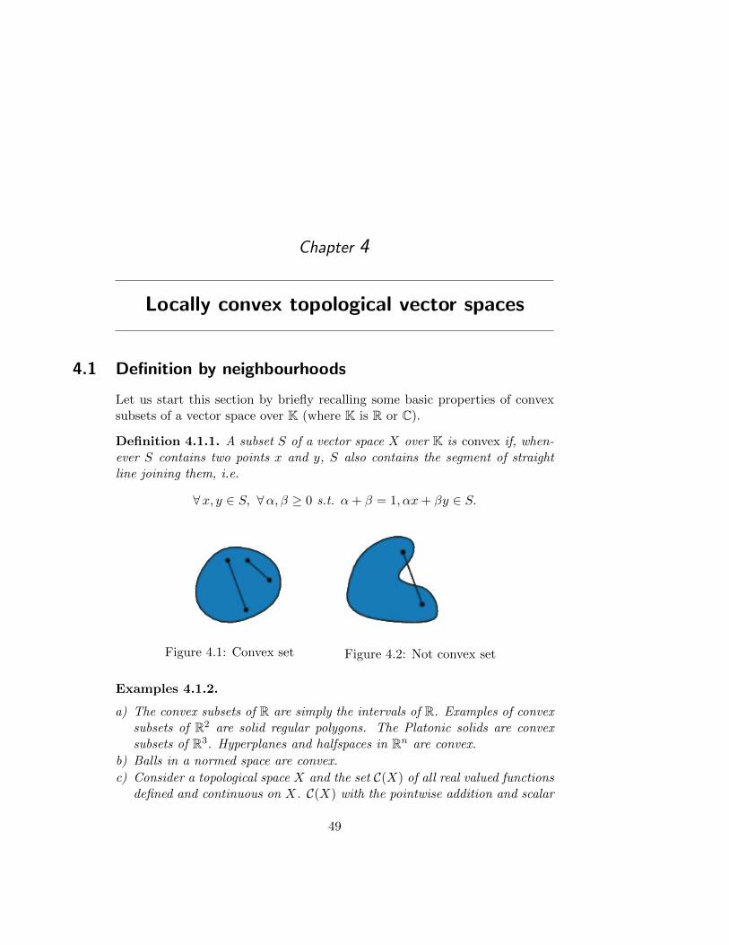
Chapter 4

Locally convex topological vector spaces

4.1 Definition by neighbourhoods

Let us start this section by briefly recalling some basic properties of convexsubsets of a vector space over K (where K is R or C).

Definition 4.1.1. A subset S of a vector space X over K is convex if, when-ever S contains two points x and y, S also contains the segment of straightline joining them, i.e.

∀x, y ∈ S, ∀α, β ≥ 0 s.t. α+ β = 1, αx+ βy ∈ S.

Figure 4.1: Convex set Figure 4.2: Not convex set

Examples 4.1.2.

a) The convex subsets of R are simply the intervals of R. Examples of convexsubsets of R2 are solid regular polygons. The Platonic solids are convexsubsets of R3. Hyperplanes and halfspaces in Rn are convex.

b) Balls in a normed space are convex.

c) Consider a topological space X and the set C(X) of all real valued functionsdefined and continuous on X. C(X) with the pointwise addition and scalar

49

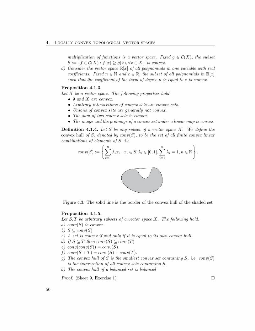
4. Locally convex topological vector spaces

multiplication of functions is a vector space. Fixed g ∈ C(X), the subsetS := f ∈ C(X) : f(x) ≥ g(x), ∀x ∈ X is convex.

d) Consider the vector space R[x] of all polynomials in one variable with realcoefficients. Fixed n ∈ N and c ∈ R, the subset of all polynomials in R[x]such that the coefficient of the term of degree n is equal to c is convex.

Proposition 4.1.3.Let X be a vector space. The following properties hold.• ∅ and X are convex.• Arbitrary intersections of convex sets are convex sets.• Unions of convex sets are generally not convex.• The sum of two convex sets is convex.• The image and the preimage of a convex set under a linear map is convex.

Definition 4.1.4. Let S be any subset of a vector space X. We define theconvex hull of S, denoted by conv(S), to be the set of all finite convex linearcombinations of elements of S, i.e.

conv(S) :=

n∑i=1

λixi : xi ∈ S, λi ∈ [0, 1],

n∑i=1

λi = 1, n ∈ N

.

Figure 4.3: The solid line is the border of the convex hull of the shaded set

Proposition 4.1.5.Let S, T be arbitrary subsets of a vector space X. The following hold.a) conv(S) is convexb) S ⊆ conv(S)c) A set is convex if and only if it is equal to its own convex hull.d) If S ⊆ T then conv(S) ⊆ conv(T )e) conv(conv(S)) = conv(S).f) conv(S + T ) = conv(S) + conv(T ).g) The convex hull of S is the smallest convex set containing S, i.e. conv(S)

is the intersection of all convex sets containing S.h) The convex hull of a balanced set is balanced


50

4.1. Definition by neighbourhoods

Definition 4.1.6. A subset S of a vector space X over K is absolutely convexif it is convex and balanced.

Let us come back now to topological vector space.

Proposition 4.1.7. The closure and the interior of convex sets in a t.v.s. areconvex sets.

Proof. Let S be a convex subset of a t.v.s. X. For any λ ∈ [0, 1], we define:

ϕλ : X ×X → X(x, y) 7→ λx+ (1− λ)y

.

Note that each ϕλ is continuous by the continuity of addition and scalarmultiplication in the t.v.s. X. Since S is convex, for any λ ∈ [0, 1] we havethat ϕλ(S × S) ⊆ S and so ϕλ(S × S) ⊆ S. The continuity of ϕλ guaranteesthat ϕλ(S × S) ⊆ ϕλ(S × S). Hence, we can conclude that ϕλ(S × S) =ϕλ(S × S) ⊆ S, i.e. S is convex.

To prove the convexity of the interior S, we must show that for any twopoints x, y ∈ S and for any λ ∈ [0, 1] the point z := ϕλ(x, y) ∈ S.

By definition of interior points of S, there exists a neighborhood U of theorigin in X such that x+U ⊆ S and y+U ⊆ S. Then, of course, the claim isthat z + U ⊆ S. This is indeed so, since for any element u ∈ U we can writez + u in the following form:

z + u = λx+ (1− λ)y + λu+ (1− λ)u = λ(x+ u) + (1− λ)(y + u)

and since both vectors x + u and y + u belong to S, so does z + u. Hence,z ∈ S which proves S is convex.

Definition 4.1.8. A subset T of a t.v.s. is called a barrel if T has the followingproperties:

1. T is absorbing2. T is absolutely convex3. T is closed

Proposition 4.1.9. Every neighborhood of the origin in a t.v.s. is containedin a neighborhood of the origin which is a barrel.

Proof.Let U be a neighbourhood of the origin and define

T (U) := conv

( ⋃λ∈K,|λ|≤1

λU

).

51


Clearly, U ⊆ T (U). Therefore, T (U) is a neighbourhood of the origin and soit is absorbing by Theorem 2.1.10. By construction, T (U) is also closed andconvex as closure of a convex set (see Proposition 4.1.7). To prove that T (U)is a barrel it remains to show that it is balanced. It is easy to see that any

point z ∈ conv

(⋃λ∈K,|λ|≤1 λU

)can be written as

z = tx+ (1− t)y

with 0 ≤ t ≤ 1, x ∈ λU and y ∈ µU , for some λ, µ ∈ K s.t. |λ| ≤ 1 and|µ| ≤ 1. Then for any ξ ∈ K with |ξ| ≤ 1 we have:

ξz = t(ξx) + (1− t)(ξy) ∈ conv

( ⋃λ∈K,|λ|≤1

λU

)

since |ξλ| ≤ 1 and |ξµ| ≤ 1. This proves that conv

(⋃λ∈K,|λ|≤1 λU

)is bal-

anced 1. Hence, by Sheet 3 Exercise 2b, its closure T (U) is also balanced.

Corollary 4.1.10. Every neighborhood of the origin in a t.v.s. is containedin a neighborhood of the origin which is absolutely convex.

Note that the converse of Proposition 4.1.9 does not hold in any t.v.s..Indeed, not every neighborhood of the origin contains another one which isa barrel. This means that not every t.v.s. has a basis of neighbourhoodconsisting of barrels. However, this is true for any locally convex t.v.s.

Definition 4.1.11. A t.v.s. X is said to be locally convex (l.c.) if there is abasis of neighborhoods of the origin in X consisting of convex sets.

Locally convex spaces are by far the most important class of t.v.s. andwe will present later on several examples of such t.v.s.. For the moment letus focus on the properties of the filter of neighbourhoods of locally convexspaces.

Proposition 4.1.12. A locally convex t.v.s. always has a basis of neighbour-hoods of the origin consisting of open absorbing absolutely convex subsets.

1One could also have directly observed that the set⋃λ∈K,|λ|≤1 λU is balanced and used

Proposition 4.1.5-h to deduce that its convex hull is balanced.

52

4.1. Definition by neighbourhoods

Proof.Let N be a neighbourhood of the origin in X. Since X is locally convex, thereexists W convex neighbourhood of the origin in X s.t.W ⊆ N . Moreover, byTheorem 2.1.10, there exists U balanced neighbourhood of the origin in X s.t.U ⊆W . The balancedness of U implies that U =

⋃λ∈K,|λ|≤1 λU . Then, using

that W is a convex set containing U , we get

O := conv

( ⋃λ∈K,|λ|≤1

λU

)= conv(U) ⊆W ⊆ N

and so O ⊆ N . Hence, the conclusion holds because O is clearly open andconvex and it is also balanced since o ∈ O and O is balanced (as we havealready showed in the proof of Proposition 4.1.9).

Similarly, we easily get that

Proposition 4.1.13. A locally convex t.v.s. always has a basis of neighbour-hoods of the origin consisting of barrels.

Proof.Let N be a neighbourhood of the origin in X. We know that every t.v.s. has abasis of closed neighbourhoods of the origin (see Sheet 3, Exercise 3a). Thenthere exists V closed neighbourhood of the origin in X s.t. V ⊆ N . Since X islocally convex, then there exists W convex neighbourhood of the origin in Xs.t. W ⊆ V . Moreover, by Theorem 2.1.10, there exists U balanced neighbour-hood of the origin in X s.t. U ⊆W . Summing up we have: U ⊆W ⊆ V ⊆ Nfor some U,W, V neighbourhoods of the origin s.t. U balanced, W convexand V closed. The balancedness of U implies that U =

⋃λ∈K,|λ|≤1 λU . Then,

using that W is a convex set containing U , we get

conv

( ⋃λ∈K,|λ|≤1

λU

)= conv(U) ⊆W

Passing to the closures and using that V we get

T (U) = conv(U) ⊆W ⊆ V = V ⊆ N.

Hence, the conclusion holds because we have already showed in Proposi-tion 4.1.9 that T (U) is a barrel neighbourhood of the origin in X.

53


We can then characterize the class of locally convex t.v.s in terms of ab-sorbing absolutely convex neighbourhoods of the origin.

Theorem 4.1.14. If X is a l.c. t.v.s. then there exists a basis B of neigh-bourhoods of the origin consisting of absorbing absolutely convex subsets s.t.

a) ∀U, V ∈ B, ∃W ∈ B s.t. W ⊆ U ∩ Vb) ∀U ∈ B, ∀ ρ > 0, ∃W ∈ B s.t. W ⊆ ρUConversely, if B is a collection of absorbing absolutely convex subsets of a vec-tor space X s.t. a) and b) hold, then there exists a unique topology compatiblewith the linear structure of X s.t. B is a basis of neighbourhoods of the originin X for this topology (which is necessarily locally convex).


In particular, the collection of all multiples ρU of an absorbing absolutelyconvex subset U of a vector space X is a basis of neighborhoods of the originfor a locally convex topology on X compatible with the linear structure (thisceases to be true, in general, if we relax the conditions on U).

4.2 Connection to seminorms

In applications it is often useful to define a locally convex space by means of asystem of seminorms. In this section we will investigate the relation betweenlocally convex t.v.s. and seminorms.

Definition 4.2.1. Let X be a vector space. A function p : X → R is called aseminorm if it satisfies the following conditions:

1. p is subadditive: ∀x, y ∈ X, p(x+ y) ≤ p(x) + p(y).

2. p is positively homogeneous: ∀x, y ∈ X, ∀λ ∈ K, p(λx) = |λ|p(x).

Definition 4.2.2. A seminorm p on a vector space X is a norm if p−1(0) =o (i.e. if p(x) = 0 implies x = o).

Proposition 4.2.3. Let p be a seminorm on a vector space X. Then thefollowing properties hold:

• p is symmetric.

• p(o) = 0.

• |p(x)− p(y)| ≤ p(x− y), ∀x, y ∈ X.

• p(x) ≥ 0, ∀x ∈ X.

• Ker(p) is a linear subspace.

54

4.2. Connection to seminorms

Proof.

• The symmetry of p directly follows from the positive homogeneity of p.Indeed, for any x ∈ X we have

p(−x) = p(−1 · x) = | − 1|p(x) = p(x).

• Using again the positive homogeneity of p we get that p(o) = p(0 · x) =0 · p(x) = 0.• For any x, y ∈ X, the subadditivity of p guarantees the following in-

equalities:

p(x) = p(x−y+y) ≤ p(x−y)+p(y) and p(y) = p(y−x+x) ≤ p(y−x)+p(x)

which establish the third property.• The previous property directly gives the nonnegativity of p. In fact, for

any x ∈ X we get

0 ≤ |p(x)− p(o)| ≤ p(x− o) = p(x).

• Let x, y ∈ Ker(p) and α, β ∈ K. Then

p(αx+ βy) ≤ |α|p(x) + |β|p(y) = 0

which implies p(αx+ βy) = 0, i.e. αx+ βy ∈ Ker(p).

Examples 4.2.4.

a) Suppose X = Rn and let M be a vector subspace of X. Set for any x ∈ X

pM (x) := infy∈M‖x− y‖

where ‖ · ‖ is the Euclidean norm, i.e. pM (x) is the distance from the pointx to M in the usual sense. If dim(M) ≥ 1 then pM is a seminorm and nota norm (M is exactly the kernel of pM ). When M = o, pM (·) = ‖ · ‖.

b) Let X be a vector space on which is defined a nonnegative sesquilinearHermitian form B : X ×X → K. Then the function

pB(x) := B(x, x)12

is a seminorm. pB is a norm if and only if B is positive definite (i.e.B(x, x) > 0, ∀x 6= o).

55


c) Let C(R) be the vector space of all real valued continuous functions on thereal line. For any bounded interval [a, b] with a, b ∈ R and a < b, we definefor any f ∈ C(R):

p[a,b](f) := supa≤t≤b

|f(t)|.

p[a,b] is a seminorm but is never a norm because it might be that f(t) = 0for all t ∈ [a, b] (and so that p[a,b](f) = 0) but f 6≡ 0. Other seminorms arethe following ones:

q(f) := |f(0)| and qp(f) :=

(∫ b

a|f(t)|pdt

) 1p

for 1 ≤ p <∞.

Note that if 0 < p < 1 then qp is not subadditive and so it is not a semi-norm.

Seminorms on vector spaces are strongly related to a special kind of func-tionals, i.e. Minkowski functionals. Let us investigate more in details such arelation. Note that we are still in the realm of vector spaces with no topology!

Definition 4.2.5. Let X be a vector space and A a non-empty subset of X.We define the Minkowski functional (or gauge) of A to be the mapping:

pA : X → Rx 7→ pA(x) := infλ > 0 : x ∈ λA

(where pA(x) =∞ if the set λ > 0 : x ∈ λA is empty).

It is then natural to ask whether there exists a class of subsets for whichthe associated Minkowski functionals are actually seminorms. The answeris positive for a class of subsets which we have already encountered in theprevious section, namely for absorbing absolutely convex subsets. Actuallywe have even more as established in the following lemma.

Notation 4.2.6. Let X be a vector space and p a seminorm on X. The sets

Up = x ∈ X : p(x) < 1 and Up = x ∈ X : p(x) ≤ 1.

are said to be, respectively, the closed and the open unit semiball of p.

Lemma 4.2.7. Let X be a vector space. If A is a non-empty subset of X whichis absorbing and absolutely convex, then the associated Minkowski functionalpA is a seminorm and UpA ⊆ A ⊆ UpA. Conversely, if q is a seminorm on Xthen Uq is an absorbing absolutely convex set and q = pUq .

56


Proof. Let A be a non-empty subset of X which is absorbing and absolutelyconvex and denote by pA the associated Minkowski functional. We want toshow that pA is a seminorm.• First of all, note that pA(x) <∞ for all x ∈ X because A is absorbing.

Indeed, by definition of absorbing set, for any x ∈ X there exists ρx > 0s.t. for all λ ∈ K with |λ| ≤ ρx we have λx ∈ A and so the set λ >0 : x ∈ λA is never empty i.e. pA has only finite nonnegative values.Moreover, since o ∈ A, we also have that o ∈ λA for any λ ∈ K and sopA(o) = infλ > 0 : o ∈ λA = 0.• The balancedness of A implies that pA is positively homogeneous. Since

we have already showed that pA(o) = 0 it remains to prove the positivehomogeneity of pA for non-null scalars. Since A is balanced we have thatfor any x ∈ X and for any ξ, λ ∈ K with ξ 6= 0 the following holds:

ξx ∈ λA if and only if x ∈ λ

|ξ|A. (4.1)

Indeed, A balanced guarantees that ξA = |ξ|A and so x ∈ λ|ξ|A is equiv-

alent to ξx ∈ λ ξ|ξ|A = λA. Using (4.1), we get that for any x ∈ X and

for any ξ ∈ K with ξ 6= 0:

pA(ξx) = infλ > 0 : ξx ∈ λA

= inf

λ > 0 : x ∈ λ

|ξ|A

= inf

|ξ| λ|ξ|

> 0 : x ∈ λ

|ξ|A

= |ξ| infµ > 0 : x ∈ µA = |ξ|pA(x).

• The convexity of A ensures the subadditivity of pA. Take x, y ∈ X. Bydefinition of Minkowski functional, for every ε > 0 there exists λ, µ > 0s.t.

λ ≤ pA(x) + ε and x ∈ λA

andµ ≤ pA(y) + ε and y ∈ µA.

Then, by the convexity of A, we obtain that λλ+µA + µ

λ+µA ⊆ A, i.e.λA+ µA ⊆ (λ+ µ)A, and therefore x+ y ∈ (λ+ µ)A. Hence:

pA(x+ y) = infδ > 0 : x+ y ∈ δA ≤ λ+ µ ≤ pA(x) + pA(y) + 2ε

which proves the subadditivity of pA since ε is arbitrary.

57


We can then conclude that pA is a seminorm. Furthermore, we have thefollowing inclusions:

UpA ⊆ A ⊆ UpA .In fact, if x ∈ UpA then pA(x) < 1 and so there exists 0 ≤ λ < 1 s.t. x ∈ λA.Since A is balanced, for such λ we have λA ⊆ A and therefore x ∈ A. On theother hand, if x ∈ A then clearly 1 ∈ λ > 0 : x ∈ λA which gives pA(x) ≤ 1and so x ∈ UpA .

Conversely, let us take any seminorm q on X. Let us first show that Uq isabsorbing and absolutely convex and then that q coincides with the Minkowskifunctional associated to Uq.• Uq is absorbing.

Let x be any point in X. If q(x) = 0 then clearly x ∈ Uq. If q(x) > 0,we can take 0 < ρ < 1

q(x) and then for any λ ∈ K s.t. |λ| ≤ ρ the

positive homogeneity of q implies that q(λx) = |λ|q(x) ≤ ρq(x) < 1, i.e.λx ∈ Uq.

• Uq is balanced.For any x ∈ Uq and for any λ ∈ K with |λ| ≤ 1, again by the positivehomogeneity of q, we get: q(λx) = |λ|q(x) ≤ q(x) < 1 i.e. λx ∈ Uq.

• Uq is convex.For any x, y ∈ Uq and any t ∈ [0, 1], by both the properties of seminorm,we have that q(tx + (1 − t)y) ≤ tq(x) + (1 − t)q(y) < t + 1 − t = 1 i.e.tx+ (1− t)y ∈ Uq.

Moreover, for any x ∈ X we easily see that

pUq(x) = infλ > 0 : x ∈ λUq = infλ > 0 : q(x) < λ = q(x).

We are now ready to see the connection between seminorms and locallyconvex t.v.s..

Definition 4.2.8. Let X be a vector space and P := pii∈I a family ofseminorms on X. The coarsest topology τP on X s.t. each pi is continuous issaid to be the topology induced or generated by the family of seminorms P.

Theorem 4.2.9. Let X be a vector space and P := pii∈I a family of semi-norms. Then the topology induced by the family P is the unique topologymaking X into a locally convex t.v.s. and having as a basis of neighbourhoodsof the origin in X the following collection:

B :=x ∈ X : pi1(x) < ε, . . . , pin(x) < ε : i1, . . . , in ∈ I, n ∈ N, ε > 0, ε ∈ R

.

Viceversa, the topology of an arbitrary locally convex t.v.s. is always inducedby a family of seminorms (often called generating).

58


Proof. Let us first show that the collection B is a basis of neighbourhoods ofthe origin for the unique topology τ making X into a locally convex t.v.s. byusing Theorem 4.1.14 and then let us prove that τ actually coincides with thetopology induced by the family P.

For any i ∈ I and any ε > 0, consider the set x ∈ X : pi(x) < ε = εUpi .This is absorbing and absolutely convex, since we have already showed abovethat Upi fulfills such properties. Therefore, any element of B is an absorbingabsolutely convex subset of X as finite intersection of absorbing absolutelyconvex sets. Moreover, both properties a) and b) of Theorem 4.1.14 are clearlysatisfied by B. Hence, Theorem 4.1.14 guarantees that there exists a uniquetopology τ on X s.t. (X, τ) is a locally convex t.v.s. and B is a basis ofneighbourhoods of the origin for τ .

Let us consider (X, τ). Then for any i ∈ I, the seminorm pi is continuous,because for any ε > 0 we have p−1

i ([0, ε[) = x ∈ X : pi(x) < ε ∈ B whichmeans that p−1

i ([0, ε[) is a neighbourhood of the origin in (X, τ). Therefore,the topology τP induced by the family P is by definition coarser than τ . Onthe other hand, each pi is also continuous w.r.t. τP and so B ⊆ τP . But B isa basis for τ , then necessarily τ is coarser than τP . Hence, τ ≡ τP .

Viceversa, let us assume that (X, τ) is a locally convex t.v.s.. Then byTheorem 4.1.14 there exists a basis N of neighbourhoods of the origin in Xconsisting of absorbing absolutely convex sets s.t. the properties a) and b)in Theorem 4.1.14 are fulfilled. W.l.o.g. we can assume that they are open.Consider now the family S := pN : N ∈ N. By Lemma 4.2.7, we know thateach pN is a seminorm and that UpN ⊆ N . Let us show that for any N ∈ Nwe have actually that N = UpN . Since any N ∈ N is open and the scalarmultiplication is continuous we have that for any x ∈ N there exists 0 < t < 1s.t. x ∈ tN and so pN (x) ≤ t < 1, i.e. x ∈ UpN .

We want to show that the topology τS induced by the family S coincideswith original topology τ on X. We know from the first part of the proof howto construct a basis for a topology induced by a family of seminorms. In fact,a basis of neighbourhoods of the origin for τS is given by

B :=

n⋂i=1

x ∈ X : pNi(x) < ε : N1, . . . , Nn ∈ N , n ∈ N, ε > 0, ε ∈ R

.

For any N ∈ N we have showed that N = UpN ∈ B so by Hausdorff criterionτ ⊆ τS . Also for any B ∈ B we have B = ∩ni=1εUpNi = ∩ni=1εNi for somen ∈ N, N1, . . . , Nn ∈ N and ε > 0. Then the property b) (of Theorem 4.1.14)forN implies that for each i = 1, . . . , n there exists Vi ∈ N s.t. Vi ⊆ εNi and soby the property a) of N we have that there exists V ∈ N s.t. V ⊆ ∩ni=1Vi ⊆ B.Hence, by Hausdorff criterion τS ⊆ τ .

59


This result justifies why several authors define a locally convex space tobe a t.v.s whose topology is induced by a family of seminorms (which is nowevidently equivalent to Definition 4.1.11)

In the previous proofs we have used some interesting properties of semiballsin a vector space. For convenience, we collect them here together with somefurther ones which we will repeatedly use in the following.

Proposition 4.2.10. Let X be a vector space and p a seminorm on X. Then:

a) Up is absorbing and absolutely convex.

b) ∀ r > 0, rUp = x ∈ X : p(x) < r = U 1rp.

c) ∀x ∈ X, x+ Up = y ∈ X : p(y − x) < 1.d) If q is also a seminorm on X then: p ≤ q if and only if Uq ⊆ Up.e) If n ∈ N and s1, . . . , sn are seminorms on X, then their maximum s defined

as s(x) := maxi=1,...,n

si(x), ∀x ∈ X is also seminorm on X and Us =⋂ni=1 Usi.

All the previous properties also hold for closed semballs.

Proof.

a) This was already proved as part of Lemma 4.2.7.

b) For any r > 0, we have

rUp = rx ∈ X : p(x) < 1 = y ∈ X :1

rp(y) < 1︸︷︷︸

U 1r p

= y ∈ X : p(y) < r.

c) For any x ∈ X, we have

x+ Up = x+ z ∈ X : p(z) < 1 = y ∈ X : p(y − x) < 1.

d) Suppose that p ≤ q and take any x ∈ Uq. Then we have q(x) < 1 andso p(x) ≤ q(x) < 1, i.e. x ∈ Up. Viceversa, suppose that Uq ⊆ Up holdsand take any x ∈ X. We have that either q(x) > 0 or q(x) = 0. In thefirst case, for any 0 < ε < 1 we get that q

(εxq(x)

)= ε < 1. Then εx

q(x) ∈ Uqwhich implies by our assumption that εx

q(x) ∈ Up i.e. p(εxq(x)

)< 1. Hence,

εp(x) < q(x) and so when ε → 1 we get p(x) ≤ q(x). If instead we are inthe second case that is when q(x) = 0, then we claim that also p(x) = 0.Indeed, if p(x) > 0 then q

(xp(x)

)= 0 and so x

p(x) ∈ Uq which implies by our

assumption that xp(x) ∈ Up, i.e. p(x) < p(x) which is a contradiction.

e) It is easy to check, using basic properties of the maximum, that the subad-ditivity and the positive homogeneity of each si imply the same propertiesfor s. In fact, for any x, y ∈ X and for any λ ∈ K we get:

60


• s(x+ y) = maxi=1,...,n

si(x+ y) ≤ maxi=1,...,n

(si(x) + si(y))

≤ maxi=1,...,n

si(x) + maxi=1,...,n

si(y) = s(x) + s(y)

• s(λx) = maxi=1,...,n

si(λx) = |λ| maxi=1,...,n

si(x) = |λ|s(x).

Moreover, if x ∈ Us then maxi=1,...,n

si(x) < 1 and so for all i = 1, . . . , n we

have si(x) < 1, i.e. x ∈⋂ni=1 Usi . Conversely, if x ∈

⋂ni=1 Usi then for all

i = 1, . . . , n we have si(x) < 1. Since s(x) is the maximum over a finitenumber of terms, it will be equal to sj(x) for some j ∈ 1, . . . , n andtherefore s(x) = sj(x) < 1, i.e. x ∈ Us.

Proposition 4.2.11. Let X be a t.v.s. and p a seminorm on X. Then thefollowing conditions are equivalent:a) the open unit semiball Up of p is an open set.b) p is continuous at the origin.c) the closed unit semiball Up of p is a barrel neighbourhood of the origin.d) p is continuous at every point.

Proof.a)⇒ b) Suppose that Up is open in the topology on X. Then for any ε > 0

we have that p−1([0, ε[) = x ∈ X : p(x) < ε = εUp is an open neighbourhoodof the origin in X. This is enough to conclude that p : X → R+ is continuousat the origin.

b)⇒ c) Suppose that p is continuous at the origin, then Up = p−1([0, 1]) isa closed neighbourhood of the origin. Since Up is also absorbing and absolutelyconvex by Proposition 4.2.10-a), Up is a barrel.

c)⇒ d) Assume that c) holds and fix o 6= x ∈ X. Using Proposition 4.2.10and Proposition 4.2.3, we get that for any ε > 0: p−1([−ε+ p(x), p(x) + ε]) =y ∈ X : |p(y) − p(x)| ≤ ε ⊇ y ∈ X : p(y − x) ≤ ε = x + εUp, whichis a closed neighbourhood of x since X is a t.v.s. and by the assumption c).Hence, p is continuous at x.

d)⇒ a) If p is continuous on X then a) holds because the preimage of anopen set under a continuous function is open and Up = p−1([0, 1[).

With such properties in our hands we are able to give a criterion to comparetwo locally convex topologies using their generating families of seminorms.

61


Theorem 4.2.12 (Comparison of l.c. topologies).Let P = pii∈I and Q = qjj∈J be two families of seminorms on the vectorspace X inducing respectively the topologies τP and τQ, which both make Xinto a locally convex t.v.s.. Then τP is finer than τQ (i.e. τQ ⊆ τP) iff

∀q ∈ Q ∃n ∈ N, i1, . . . , in ∈ I, C > 0 s.t. Cq(x) ≤ maxk=1,...,n

pik(x), ∀x ∈ X.

(4.2)Proof.Let us first recall that, by Theorem 4.2.9, we have that

BP := n⋂k=1

εUpik : i1, . . . , in ∈ I, n ∈ N, ε > 0, ε ∈ R

and

BQ := n⋂k=1

εUqjk : j1, . . . , jn ∈ J, n ∈ N, ε > 0, ε ∈ R.

are respectively bases of neighbourhoods of the origin for τP and τQ.By using Proposition 4.2.10, the condition (4.2) can be rewritten as

∀q ∈ Q, ∃n ∈ N, i1, . . . , in ∈ I, C > 0 s.t. C

n⋂k=1

Upik ⊆ Uq.

which means that

∀q ∈ Q, ∃ Bq ∈ BP s.t. Bq ⊆ Uq. (4.3)

since C⋂nk=1 Upik ∈ BP .

Condition (4.3) means that for any q ∈ Q the set Uq ∈ τP , which byProposition 4.2.11 is equivalent to say that q is continuous w.r.t. τP . Bydefinition of τQ, this gives that τQ ⊆ τP . 2

2Alternate proof without using Prop 4.2.11. (Sheet 10, Exercise 1)Suppose that (4.2) holds and take any B′ ∈ BQ, i.e. B′ =

⋂mk=1 εUqjk

for somem ∈ N, j1, . . . , jn ∈ J and 0 < ε ∈ R. Then, by using m times the condition (4.3),we obtain that there exist B1, . . . , Bm ∈ BP such that ∀k ∈ 1, . . . ,m, Bk ⊆ Uqjk

.

Hence,⋂m

k=1Bi ⊆⋂m

k=1 Uqjk. Multiplying by ε both sides of the inclusion, we get

B′ ⊇ ε⋂m

k=1Bi ∈ BP and so, by Hausdorff criterion (see Theorem 1.1.16) τQ ⊆ τP .

Conversely, suppose that τP is finer than τQ and take any q ∈ Q. Since Uq ∈ BQ,

by Hausdorff criterion, we get that there exists B ∈ BP s.t. B ⊆ Uq. Now such B will

be of the form B =⋂n

k=1 εUpikfor some n ∈ N, i1, . . . , in ∈ I and 0 < ε ∈ R. Then,

Proposition 4.2.10 gives that B = εU maxk=1,...,n

pik⊆ Uq, i.e. U max

k=1,...,npik⊆ Uεq which is

equivalent to εq(x) ≤ maxk=1,...,n

pik(x), ∀x ∈ X.

62


This theorem allows us to easily see that the topology induced by a familyof seminorms on a vector space does not change if we close the family undertaking the maximum of finitely many of its elements. Indeed, the followingresult holds.

Proposition 4.2.13. Let P := pii∈I be a family of seminorms on a vectorspace X and Q :=

maxi∈B

pi : ∅ 6= B ⊆ I with B finite

. Then Q is a family

of seminorms and τP = τQ, where τP and τQ denote the topology induced onX by P and Q, respectively.

Proof.First of all let us note that, by Proposition 4.2.10, Q is a family of seminorms.On the one hand, since P ⊆ Q, by definition of induced topology we haveτP ⊆ τQ. On the other hand, for any q ∈ Q we have q = max

i∈Bpi for some

∅ 6= B ⊆ I finite. Then (4.2) is fulfilled for n = |B| (where |B| denotes thecardinality of the finite set B), i1, . . . , in being the n elements of B and forany 0 < C ≤ 1. Hence, by Theorem 4.2.12, τQ ⊆ τP .

This fact can be used to show the following very useful property of locallyconvex t.v.s.

Proposition 4.2.14. The topology of a locally convex t.v.s. can be alwaysinduced by a directed family of seminorms.

Definition 4.2.15. A family Q := qjj∈J of seminorms on a vector spaceX is said to be directed if

∀ j1, j2 ∈ J, ∃ j ∈ J,C > 0 s.t. Cqj(x) ≥ maxqj1(x), qj2(x), ∀x ∈ X (4.4)

or equivalently by induction if

∀ n ∈ N, j1, . . . , jn ∈ J, ∃ j ∈ J,C > 0 s.t. Cqj(x) ≥ maxk=1,...,n

qjk(x), ∀x ∈ X.

Proof. of Proposition 4.2.14Let (X, τ) be a locally convex t.v.s.. By Theorem 4.2.9, we have that thereexists a family of seminorms P := pii∈I on X s.t. τ = τP . Let us define Qas the collection obtained by forming the maximum of finitely many elementsof P, i.e. Q :=

maxi∈B

pi : ∅ 6= B ⊆ I with B finite

. By Proposition 4.2.13,

Q is a family of seminorms and we have that τP = τQ. We claim that Q isdirected.

63


Let q, q′ ∈ Q, i.e. q := maxi∈B

pi and q′ := maxi∈B′

pi for some non-empty finite

subsets B,B′ of I. Let us define q′′ := maxi∈B∪B′

pi. Then q′′ ∈ Q and for any

C ≥ 1 we have that (4.4) is satisfied, because we get that for any x ∈ X

Cq′′(x) = C max

maxi∈B

pi(x),maxi∈B′

pi(x)

≥ maxq(x), q′(x).

Hence, Q is directed.

It is possible to show (Sheet 10, Exercise 2) that a basis of neighbourhoodsof the origin for the l.c. topology τQ induced by a directed family of seminormsQ is given by:

Bd := rUq : q ∈ Q, r > 0. (4.5)

4.3 Hausdorff locally convex t.v.s

In Section 2.2, we gave some characterization of Hausdorff t.v.s. which canof course be applied to establish whether a locally convex t.v.s. is Hausdorffor not. However, in this section we aim to provide necessary and sufficientconditions bearing only on the family of seminorms generating a locally convextopology for being a Hausdorff topology.

Definition 4.3.1.A family of seminorms P := pii∈I on a vector space X is said to be sepa-rating if

∀x ∈ X \ o,∃ i ∈ I s.t. pi(x) 6= 0. (4.6)

Note that the separation condition (4.6) is equivalent to

pi(x) = 0, ∀i ∈ I ⇒ x = o

which by using Proposition 4.2.10 can be rewritten as⋂i∈I,c>0

cUpi = o,

since pi(x) = 0 is equivalent to say that pi(x) < c, for all c > 0.

64

4.3. Hausdorff locally convex t.v.s

Lemma 4.3.2. Let τP be the topology induced by a separating family of semi-norms P := (pi)i∈I on a vector space X. Then τP is a Hausdorff topology.

Proof. Let x, y ∈ X be s.t. x 6= y. Since P is separating, ∃ i ∈ I s.t.pi(x− y) 6= 0. Then ∃ ε > 0 s.t. pi(x− y) = 2ε. Let us define Vx := u ∈ X |pi(x− u) < ε and Vy := u ∈ X | pi(y − u) < ε. By Proposition 4.2.10, weget that Vx = x + εUpi and Vy = y + εUpi . Since Theorem 4.2.9 guaranteesthat (X, τP) is a t.v.s. where the set εUpi is a neighbourhood of the origin, Vxand Vy are neighbourhoods of x and y, respectively. They are clearly disjoint.Indeed, if there would exist u ∈ Vx ∩ Vy then

pi(x− y) = pi(x− u+ u− y) ≤ pi(x− u) + pi(u− y) < 2ε

which is a contradiction.

Proposition 4.3.3. A locally convex t.v.s. is Hausdorff if and only if itstopology can be induced by a separating family of seminorms.

Proof. Let (X, τ) be a locally convex t.v.s.. Then we know that there alwaysexists a basis N of neighbourhoods of the origin in X consisting of openabsorbing absolutely convex sets. Moreover, in Theorem 4.2.9, we have showedthat τ = τP where P is the family of seminorms given by the Minkowskifunctionals of sets in N , i.e. P := pN : N ∈ N, and also that for eachN ∈ N we have N = UpN .

Suppose that (X, τ) is also Hausdorff. Then Proposition 2.2.3 ensures thatfor any x ∈ X with x 6= o there exists a neighbourhood V of the origin in Xs.t. x /∈ V . This implies that there exists at least N ∈ N s.t. x /∈ N 3. Hence,x /∈ N = UpN means that pN (x) ≥ 1 and so pN (x) 6= 0, i.e. P is separating.

Conversely, if τ is induced by a separating family of seminorms P, i.e.τ = τP , then Lemma 4.3.2 ensures that X is Hausdorff.

Examples 4.3.4.

1. Every normed space is a Hausdorff locally convex space, since every normis a seminorm satisfying the separation property. Therefore, every Ba-nach space is a complete Hausdorff locally convex space.

3Since N is a basis of neighbourhoods of the origin, ∃ N ∈ N s.t. N ⊆ V . If x wouldbelong to all elements of the basis then in particular it would be x ∈ N and so also x ∈ V ,contradiction.

65


2. Every family of seminorms on a vector space containing a norm inducesa Hausdorff locally convex topology.

3. Given an open subset Ω of Rd with the euclidean topology, the space C(Ω)of real valued continuous functions on Ω with the so-called topology ofuniform convergence on compact sets is a locally convex t.v.s.. Thistopology is defined by the family P of all the seminorms on C(Ω) givenby

pK(f) := maxx∈K|f(x)|, ∀K ⊂ Ω compact .

Moreover, (C(Ω), τP) is Hausdorff, because the family P is clearly sepa-rating. In fact, if pK(f) = 0, ∀K compact subsets of Ω then in particularpx(f) = |f(x)| = 0 ∀x ∈ Ω, which implies f ≡ 0 on Ω.

More generally, for any X locally compact we have that C(X) with thetopology of uniform convergence on compact subsets of X is a locallyconvex Hausdorff t.v.s.

To introduce two other examples of l.c. Hausdorff t.v.s. we need to recallsome standard general notations. Let N0 be the set of all non-negative integers.For any x = (x1, . . . , xd) ∈ Rd and α = (α1, . . . , αd) ∈ Nd0 one defines xα :=xα1

1 · · ·xαdd . For any β ∈ Nd0, the symbol Dβ denotes the partial derivative of

order |β| where |β| :=∑d

i=1 βi, i.e.

Dβ :=∂|β|

∂xβ11 · · · ∂xβdd

=∂β1

∂xβ11

· · · ∂βd

∂xβdd.

Examples 4.3.5.

1. Let Ω ⊆ Rd open in the euclidean topology. For any k ∈ N0, let Ck(Ω) bethe set of all real valued k−times continuously differentiable functionson Ω, i.e. all the derivatives of f of order ≤ k exist (at every point of Ω)and are continuous functions in Ω. Clearly, when k = 0 we get the setC(Ω) of all real valued continuous functions on Ω and when k = ∞ weget the so-called set of all infinitely differentiable functions or smoothfunctions on Ω. For any k ∈ N0, Ck(Ω) (with pointwise addition andscalar multiplication) is a vector space over R. The topology given bythe following family of seminorms on Ck(Ω):

pm,K(f) := supβ∈Nd0|β|≤m

supx∈K

∣∣∣(Dβf)(x)∣∣∣ , ∀K ⊆ Ω compact,∀m ∈ 0, 1, . . . , k,

makes Ck(Ω) into a locally convex Hausdorff t.v.s.. (Note that whenk =∞ we have m ∈ N0.)

66

4.4. The finest locally convex topology

2. The Schwartz space or space of rapidly decreasing functions on Rd isdefined as the set S(Rd) of all real-valued functions which are definedand infinitely differentiable on Rd and which have the additional property(regulating their growth at infinity) that all their derivatives tend to zeroat infinity faster than any inverse power of x, i.e.

S(Rd) :=

f ∈ C∞(Rd) : sup

x∈Rd

∣∣∣xαDβf(x)∣∣∣ <∞, ∀α, β ∈ Nd0

.

(For example, any smooth function f with compact support in Rd isin S(Rd), since any derivative of f is continuous and supported on acompact subset of Rd, so xα(Dβf(x)) has a maximum in Rd by theextreme value theorem.)

The Schwartz space S(Rd) is a vector space over R and the topologygiven by the family Q of seminorms on S(Rd):

qα,β(f) := supx∈Rd

∣∣∣xαDβf(x)∣∣∣ , ∀α, β ∈ Nd0

makes S(Rd) into a locally convex Hausdorff t.v.s.. Indeed, the family isclearly separating, because if qα,β(f) = 0, ∀α, β ∈ Nd0 then in particularqo,o(f) = supx∈Rd |f(x)| = 0 ∀x ∈ Rd, which implies f ≡ 0 on Rd.Note that S(Rd) is a linear subspace of C∞(Rd), but its topology τQon S(Rd) is finer than the subspace topology induced on it by C∞(Rd).(Sheet 10, Exercise 1)

4.4 The finest locally convex topology

In the previous sections we have seen how to generate topologies on a vectorspace which makes it into a locally convex t.v.s.. Among all of them, there isthe finest one (i.e. the one having the largest number of open sets) which isusually called the finest locally convex topology on the given vector space.

Proposition 4.4.1. The finest locally convex topology on a vector space X isthe topology induced by the family of all seminorms on X and it is a Hausdorfftopology.

Proof.Let us denote by S the family of all seminorms on the vector space X. ByTheorem 4.2.9, we know that the topology τS induced by S makes X into alocally convex t.v.s. We claim that τS is the finest locally convex topology. In

67


fact, if there was a finer locally convex topology τ (i.e. if τS ⊆ τ with (X, τ)locally convex t.v.s.) then Theorem 4.2.9 would give that τ is also induced bya family P of seminorms. But surely P ⊆ S and so τ = τP ⊆ τS by definitionof induced topology. Hence, τ = τS .

It remains to show that (X, τS) is Hausdorff. By Lemma 4.3.2, it is enoughto prove that S is separating. Let x ∈ X \ o and let B be an algebraic basisof the vector space X containing x. Define the linear functional L : X → R asL(x) = 1 and L(y) = 0 for all y ∈ B \ x. Then it is easy to see that s := |L|is a seminorm, so s ∈ S and s(x) 6= 0, which proves that S is separating.

An alternative way of describing the finest locally convex topology on avector space X without using the seminorms is the following:

Proposition 4.4.2. The collection of all absorbing absolutely convex sets ofa vector space X is a basis of neighbourhoods of the origin for the finest locallyconvex topology on X.

Proof. Let τmax be the finest locally convex topology onX andA the collectionof all absorbing absolutely convex sets of X. By Theorem 4.1.14, we knowthat every locally convex t.v.s. has a basis of neighbourhood of the originconsisting of absorbing absolutely convex subsets of X. Then clearly thebasis of neighbourhoods of the origin Bmax of τmax is contained in A. Hence,τmax ⊆ τ where τ denote the topology generated by A. On the other hand,A fulfills all the properties required in Theorem 4.1.14 and so τ also makesX into a locally convex t.v.s.. Hence, by definition of finest locally convextopology, τ ⊆ τmax.

This result can be clearly proved also using the Proposition 4.4.1 andthe correspondence between Minkowski functionals and absorbing absolutelyconvex subsets of X introduced in the Section 4.2.

Proposition 4.4.3. Every linear functional on a vector space X is continuousw.r.t. the finest locally convex topology on X.

Proof. Let L : X → K be a linear functional on a vector space X. For anyε > 0, we denote by Bε(0) the open ball in K of radius ε and center 0 ∈ K,i.e. Bε(0) := k ∈ K : |k| < ε. Then we have that L−1(Bε(0)) = x ∈ X :|L(x)| < ε. It is easy to verify that the latter is an absorbing absolutelyconvex subset of X and so, by Proposition 4.4.2, it is a neighbourhood of theorigin in the finest locally convex topology on X. Hence L is continuous atthe origin and so, by Proposition 2.1.15-3), L is continuous everywhere in X.

68

4.5. Direct limit topology on a countable dimensional t.v.s.

4.5 Direct limit topology on a countable dimensional t.v.s.

In this section we are going to give an important example of finest locallyconvex topology on an infinite dimensional vector space, namely the directlimit topology on any countable dimensional vector space. For simplicity, weare going to focus on R−vector spaces.

Definition 4.5.1. Let X be an infinite dimensional vector space whose di-mension is countable. The direct limit topology (or finite topology) τf on Xis defined as follows:U ⊆ X is open in τf iff U ∩ W is open in the euclidean topology on W ,∀W ⊂ X with dim(W ) <∞.Equivalently, if we fix a Hamel basis xnn∈N of X and if for any n ∈ N weset Xn := spanx1, . . . , xn s.t. X =

⋃∞i=1Xi and X1 ⊆ . . . ⊆ Xn ⊆ . . ., then

U ⊆ X is open in τf iff U ∩ Xi is open in the euclidean topology on Vi forevery i ∈ N.

Theorem 4.5.2. Let X be an infinite dimensional vector space whose dimen-sion is countable endowed with the finite topology τf . Then:a) (X, τf ) is a Hausdorff locally convex t.v.s.b) τf is the finest locally convex topology on X

Proof.a) We leave to the reader the proof of the fact that τf is compatible with thelinear structure of X (Sheet 10, Exercise 3) and we focus instead on provingthat τf is a locally convex topology. To this aim we are going to show thatfor any open neighbourhood U of the origin in (X, τf ) there exists an openconvex neighbourhood U ′ ⊆ U .

Let xii∈N be an R-basis for X and set Xn := spanx1, . . . , xn for anyn ∈ N. We proceed (by induction on n ∈ N) to construct an increasingsequence Cn ⊆ U ∩Xn of convex subsets as follows:• For n = 1: Since U ∩X1 is open in X1 = Rx1, we have that there existsa1 ∈ R, a1 > 0 such that C1 :=

λ1x1 | − a1 ≤ λ1 ≤ a1

⊆ U ∩X1.

• Inductive assumption on n: We assume we have found a1, . . . , an ∈ R+

such that Cn :=λ1x1 + . . .+ λnxn | − ai ≤ λi ≤ ai ; i ∈ 1, . . . , n

⊆

U ∩Xn. Note that Cn is closed (in Xn, as well as) in Xn+1.• For n+ 1: We claim ∃ an+1 > 0, an+1 ∈ R such that

Cn+1 :=λ1x1+. . .+λnxn+λn+1xn+1|−ai ≤ λi ≤ ai ; i ∈ 1, . . . , n+

1⊆ U ∩Xn+1.

Proof of claim: If the claim does not hold, then ∀ N ∈ N ∃ xN ∈ Xn+1

s.t.xN = λN1 x1 + . . . λNn xn + λNn+1xn+1

69


with −ai ≤ λNi ≤ ai for i ∈ 1, . . . , n, − 1

N≤ λNn+1 ≤

1

Nand xN /∈ U .

But xN has form xN = λN1 x1 + . . .+ λNn xn︸︷︷︸∈ Cn

+λNn+1xn+1, so xNN∈N

is a bounded sequence in Xn+1\U . Therefore, we can find a subsequencexNjj∈N which is convergent as j → ∞ to x ∈ Cn ⊆ U (since Cn isclosed in Xn+1 and the n+1−th component of xNj tends to 0 as j →∞).Hence, the sequence xNjj∈N ⊆ Xn+1 \ U converges to x ∈ U but thiscontradicts the fact that Xn+1 \ U is closed in Xn+1. This establishesthe claim.

Now for any n ∈ N consider

Dn :=λ1x1 + . . .+ λnxn | − ai < λi < ai ; i ∈ 1, . . . , n

,

then Dn ⊂ Cn ⊆ U ∩Xn is open and convex in Xn. Then U ′ := ∪n∈NDn isan open and convex neighbourhood of the origin in (X, τf ) and U ′ ⊆ U .

b) Let us finally show that τf is actually the finest locally convex topologyτmax on X. Since we have already showed that τf is a l.c. topology on X,clearly we have τf ⊆ τmax by definition of finest l.c. topology on X.

Conversely, let us consider U ⊆ X open in τmax. We want to show thatU is open in τf , i.e. W ∩ U is open in the euclidean topology on W forany finite dimensional subspace W of X. Now each W inherits τmax fromX. Let us denote by τWmax the subspace topology induced by (X, τmax) onW . By definition of subspace topology, we have that W ∩ U is open in τWmax.Moreover, by Proposition 4.4.1, we know that (X, τmax) is a Hausdorff t.v.s.and so (W, τWmax) is a finite dimensional Hausdorff t.v.s. (see by Proposition2.1.15-1). Therefore, τWmax has to coincide with the euclidean topology byTheorem 3.1.1 and, consequently, W ∩U is open w.r.t. the euclidean topologyon W .

We actually already know a concrete example of countable dimensionalspace with the finite topology:

Example 4.5.3. Let n ∈ N and x = (x1, . . . , xn). Denote by R[x] the spaceof polynomials in the n variables x1, . . . , xn with real coefficients and by

Rd[x] := f ∈ R[x]|deg f ≤ d, d ∈ N0,

then R[x] :=⋃∞d=0 Rd[x]. The finite topology τf on R[x] is then given by:

U ⊆ R[x] is open in τf iff ∀d ∈ N0, U ∩ Rd[x] is open in Rd[x] with theeuclidean topology.

70

4.6. Continuity of linear mappings on locally convex spaces

4.6 Continuity of linear mappings on locally convex spaces

Since locally convex spaces are a particular class of topological vector spaces,the natural functions to be considered on this spaces are continuous linearmaps. In this section, we present a necessary and sufficient condition forthe continuity of a linear map between two l.c. spaces, bearing only on theseminorms inducing the two topologies.

For simplicity, let us start with linear functionals on a l.c. space. Recallthat for us K = R or K = C endowed with the euclidean topology given bythe absolute value | · |. In this section, for any ε > 0 we denote by Bε(0) theopen ball in K of radius ε and center 0 ∈ K i.e. Bε(0) := k ∈ K : |k| < ε.

Proposition 4.6.1. Let τ be a locally convex topology on a vector space Xgenerated by a directed family Q of seminorms on X. Then L : X → K is a τ -continuous linear functional iff there exists q ∈ Q such that L is q-continuous,i.e.

∃q ∈ Q,∃C > 0 s.t. |L(x)| ≤ Cq(x), ∀x ∈ X. (4.7)

Proof.Let us first observe that since X and K are both t.v.s. by Proposition 2.1.15-3)the continuity of L is equivalent to its continuity at the origin. Therefore, itis enough to prove the criterion for the continuity of L at the origin.

(⇒) Suppose that L is τ -continuous at the origin in X. Then we have thatL−1(B1(0)) = x ∈ X : |L(x)| < 1 is an open neighbourhood of the origin in(X, τ). Since the family Q inducing τ is directed, a basis of neighbourhoodof the origin in (X, τ) is given by Bd as in (4.5). Therefore, ∃B ∈ Bd s.t.B ⊆ L−1(B1(0)), i.e.

∃ q ∈ Q, ∃ r > 0 s.t. rUq ⊆ L−1(B1(0)). (4.8)

Then for any ε > 0 we get rεUq ⊆ εL−1(B1(0)) = L−1(Bε(0)). This provesthat L is q−continuous at the origin, because rεUq is clearly an open neigh-bourhood of the origin in X w.r.t. the topology generated by the single semi-norm q.

(⇐) Suppose that there exists q ∈ Q s.t. L is q-continuous in X. Then,since τ is the topology induced by the whole family Q which is finer thanthe one induced by the single seminorm q, we clearly have that L is alsoτ−continuous.

Note that by simply observing that |L| is a seminorm and by using Propo-sition 4.2.10 we get that (4.7) is equivalent to (4.8) and so to the q-continuityof L at the origin.

71


By using this result together with Proposition 4.2.14 we get the following.

Corollary 4.6.2. Let τ be a locally convex topology on a vector space Xgenerated by a family P := pii∈I of seminorms on X. Then L : X → K isa τ -continuous linear functional iff there exist n ∈ N, i1, . . . , in ∈ I such thatL is

(max

k=1,...,npik)-continuous, i.e.

∃n ∈ N, ∃ i1, . . . , in ∈ I, ∃C > 0 s.t. |L(x)| ≤ C maxk=1,...,n

pik(x), ∀x ∈ X.

The proof of Proposition 4.6.1 can be easily modified to get the followingmore general criterion for the continuity of any linear map between two locallyconvex spaces.

Theorem 4.6.3. Let X and Y be two locally convex t.v.s. whose topologiesare respectively generated by the families P and Q of seminorms on X. Thenf : X → Y linear is continuous iff

∀ q ∈ Q, ∃n ∈ N,∃ p1, . . . , pn ∈ P, ∃C > 0 : q(f(x)) ≤ C maxi=1,...,n

pi(x), ∀x ∈ X.

Proof. (Exercise)

72

Chapter 5

The Hahn-Banach Theoremand its applications

5.1 The Hahn-Banach Theorem

One of the most important results in the theory of t.v.s. is the Hahn-Banachtheorem (HBT). It is named for Hans Hahn and Stefan Banach who provedthis theorem independently in the late 1920s, dealing with the problem ofextending continuous linear functionals defined on a subspace of a seminormedvector space to the whole space. We will see that actually this extensionproblem can be reduced to the problem of separating by a closed hyperplanea convex open set and an affine submanifold (the image by a translation of alinear subspace) which do not intersect. Indeed, there are two main versionsof HBT showing respectively the analytic and the geometric side of this result.

Before stating these two versions of HBT, let us recall the notion of hy-perplane in a vector space (we always consider vector spaces over the fieldK which is either R or C). A hyperplane H in a vector space X over K isa maximal proper linear subspace of X or, equivalently, a linear subspace ofcodimension one, i.e. dimX/H = 1. Another equivalent formulation is that ahyperplane is a set of the form ϕ−1(0) for some linear functional ϕ : X → Knot identically zero. The translation by a non-null vector of a hyperplane willbe called affine hyperplane.

Theorem 5.1.1 (Analytic form of Hahn-Banach theorem ).Let p be a seminorm on a vector space X over K, M a linear subspace of X,and f a linear functional on M such that

|f(x)| ≤ p(x), ∀x ∈M. (5.1)

There exists a linear functional f on X extending f , i.e. f(x) = f(x) ∀x ∈M ,and such that

|f(x)| ≤ p(x), ∀x ∈ X. (5.2)

73

5. The Hahn-Banach Theorem and its applications

Theorem 5.1.2 (Geometric form of Hahn-Banach theorem ).Let X be a topological vector space over K, N a linear subspace of X, and Ωa convex open subset of X such that N ∩ Ω = ∅. Then there exists a closedhyperplane H of X such that

N ⊆ H and H ∩ Ω = ∅. (5.3)

It should be remarked that the vector space X does not apparently carryany topology in Theorem 5.1.1, but actually the datum of a seminorm on Xis equivalent to the datum of the topology induced by this seminorm. It isthen clear that the conditions (5.1) and (5.2) imply the p−continuity of thefunctions f and f , respectively.

Let us also stress the fact that in Theorem 5.1.2 neither local convexity northe Hausdorff separation property are assumed on the t.v.s. X. Moreover, it iseasy to see that the geometric form of HBT could have been stated also in anaffine setting, namely starting with any affine submanifold N of X which doesnot intersect the open convex subset Ω and getting a closed affine hyperplanefulfilling (5.3).

We first prove Theorem 5.1.2 and then show how to derive from this theanalytic form Theorem 5.1.1.

Before starting the proof, let us fix one more definition. A cone C in avector space X over R is a subset of X which is closed under addition andmultiplication by positive scalars.

Proof. Theorem 5.1.2We assume that Ω 6= ∅, otherwise there is nothing to prove.

1) Existence of a linear subspace H of X maximal for (5.3).This first part of the proof is quite simple and consists in a straightforwardapplication of Zorns lemma. In fact, consider the family F of all the linearsubspaces L of X such that

N ⊆ L and L ∩ Ω = ∅. (5.4)

F is clearly non-empty since N belongs to it by assumption. If we take now atotally ordered subfamily C of F (totally ordered for the inclusion relation ⊆),then the union of all the linear subspaces belonging to C is a linear subspace ofX having the properties in (5.4). Hence, we can apply Zorn’s lemma appliesand conclude that there exists at least a maximal element H in F .

2) H is closed in X.The fact that H and Ω do not intersect gives that H is contained in the

74

5.1. The Hahn-Banach Theorem

complement of Ω in X. This implies that also its closure H does not intersectΩ. Indeed, since Ω is open, we get

H ⊆ X \ Ω = X \ Ω.

Then H is a linear subspace (as closure of a linear subspace) of X, which isdisjoint from Ω and which contains H and so N , i.e. H ∈ F . Hence, as H ismaximal in F , it must coincide with its closure. Note that the fact that His closed guarantees that the quotient space X/H is a Hausdorff t.v.s. (seeProposition 2.3.5).

3) H is an hyperplaneWe want to show that H is a hyperplane, i.e. that dim(X/H) = 1. To thisaim we distinguish the two cases when K = R and when K = C.

3.1) Case K = RLet φ : X → X/H be the canonical map. Since φ is an open linear mapping(see Proposition 2.3.2), φ(Ω) is an open convex subset of X/H. Also we havethat φ(Ω) does not contain the origin o of X/H. Indeed, if o ∈ φ(Ω) holds,then there would exist x ∈ Ω s.t. φ(x) = o and so x ∈ H, which wouldcontradict the assumption H ∩ Ω = ∅. Let us set:

A =⋃λ>0

λφ(Ω).

Then the subset A of X/H is open, convex and it is a cone which does notcontain the origin o.

Let us observe that X/H has at least dimension 1. If dim(X/H) = 0 thenX/H = o and so X = H which contradicts the fact that Ω does not intersectH (recall that we assumed Ω is non-empty). Suppose that dim(X/H) ≥ 2,then to get our conclusion it will suffice to show the following claims:

Claim 1: The boundary ∂A of A must contain at least one point x 6= o.Claim 2: The point −x cannot belong to A.

In fact, once Claim 1 is established, we have that x /∈ A, because x ∈ ∂A andA is open. This together with Claim 2 gives that both x and −x belong to thecomplement of A in X/H and, therefore, so does the straight line L definedby these two points. (If there was a point y ∈ L∩A then any positive multipleof y would belong to L ∩ A, as A is a cone. Hence, for some λ > 0 we wouldhave x = λy ∈ L ∩A, which contradicts the fact that x /∈ A.) Then:• φ−1(L) is a linear subspace of X• φ−1(L) ∩ Ω = ∅, since L ∩A = ∅• φ−1(L) ) H because o = φ(H) ⊆ L but L 6= o since x 6= o is in L.

This contradicts the maximality of H and so dim(X/H) = 1.To complete the proof of 3.1) let us show the two claims.

75


Proof. of Claim 1Suppose that ∂A = o. This means that A has empty boundary in the set(X/H) \ o and so that A is a connected component of (X/H) \ o. Sincedim(X/H) ≥ 2, the space (X/H) \ o is arc-connected and so it is itself aconnected space. Hence, A = (X/H) \ o which contradicts the convexity ofA since (X/H) \ o is clearly not convex.

Proof. of Claim 2Suppose −x ∈ A. Then, as A is open, there is a neighborhood V of −xentirely contained in A. This implies that −V is a neighborhood of x. Sincex is a boundary point of A, there exists y ∈ (−V )∩A. But then −y ∈ V ⊂ Aand so, by the convexity of A, the whole line segment between y and −y iscontained in A, in particular o, which contradicts the definition of A.

3.2) Case K = CAlthough here we are consider the scalars to be the complex numbers, wemay view X as a vector space over the real numbers and it is obvious that itstopology, as originally given, is still compatible with its linear structure. Bystep 3.1) above, we know that there exists a real hyperplane H0 of X whichcontains N and does not intersect Ω. By a real hyperplane, we mean thatH0 is a linear subspace of X viewed as a vector space over the field of realnumbers such that dimR(X/H) = 1.

Now it is easy to see that iN = N (here i =√−1). Hence, setting

H := H0 ∩ iH0, we have that N ⊆ H and H ∩ Ω = ∅. Then to complete theproof it remains to show that this H is a complex hyperplane. It is obviouslya complex linear subspace of X and its real codimension is ≥ 1 and ≤ 2 (sincethe intersection of two distinct hyperplanes is always a linear subspace withcodimension two). Hence, its complex codimension is equal to one.

Proof. Theorem 5.1.1Let p be a seminorm on the vector space X, M a linear subspace of X, and fa linear functional defined on M fulfilling (5.1). As already remarked before,this means that f is continuous on M w.r.t. the topology induced by p on X(which makes X a l.c. t.v.s.).

Consider the subset N := x ∈ M : f(x) = 1. Taking any vectorx0 ∈ N , it is easy to see that N − x0 = Ker(f) (i.e. the kernel of f inM), which is a hyperplane of M and so a linear subspace of X. Therefore,setting M0 := N − x0, we have the following decomposition of M :

M = M0 ⊕Kx0,

76

5.2. Applications of Hahn-Banach theorem

where Kx0 is the one-dimensional linear subspace through x0. In other words

∀x ∈M, ∃!λ ∈ K, y ∈M0 : x = y + λx0.

Then

∀x ∈M, f(x) = f(y) + λf(x0) = λf(x0) = λ,

which means that the values of f on M are completely determined by the oneson N . Consider now the open unit semiball of p:

U := Up = x ∈ X : p(x) < 1,

which we know being an open convex subset of X endowed with the topologyinduced by p. Then N ∩U = ∅ because if there was x ∈ N ∩U then p(x) < 1and f(x) = 1, which contradict (5.1).

By Theorem 5.1.2 (affine version), there exists a closed affine hyperplaneH of X with the property that N ⊆ H and H ∩ U = ∅. Then H − x0

is a hyperplane and so the kernel of a continuous linear functional f on Xnon-identically zero.

Arguing as before (consider here the decomposition X = (H−x0)⊕Kx0),we can deduce that the values of f on X are completely determined by theones on N and so on H (because for any h ∈ H we have h−x0 ∈ Ker(f) andso f(h) − f(x0) = f(h − x0) = 0). Since f 6≡ 0, we have that f(x0) 6= 0 andw.l.o.g. we can assume f(x0) = 1 i.e. f ≡ 1 on H. Therefore, for any x ∈Mthere exist unique λ ∈ K and y ∈ N − x0 ⊆ H − x0 s.t. x = y + λx0, we getthat:

f(x) = λf(x0) = λ = λf(x0) = f(x),

i.e. f is the restriction of f to M . Furthermore, the fact that H∩U = ∅ meansthat f(x) = 1 implies p(x) ≥ 1. Then for any y ∈ X s.t. f(y) 6= 0 we have

that: f(

y

f(y)

)= 1 and so that p

(y

f(y)

)≥ 1 which implies that |f(y)| ≤ p(y).

The latter obviously holds for f(y) = 0. Hence, (5.2) is established.

5.2 Applications of Hahn-Banach theorem

The Hahn-Banach theorem is frequently applied in analysis, algebra and ge-ometry, as will be seen in the forthcoming course. We will briefly indicatein this section some applications of this theorem to problems of separation ofconvex sets and to the multivariate moment problem. From now on we willfocus on t.v.s. over the field of real numbers.

77


5.2.1 Separation of convex subsets of a real t.v.s.

Let X t.v.s.over the field of real numbers and H be a closed affine hyperplaneof X. We say that two disjoint subsets A and B of X are separated by Hif A is contained in one of the two closed half-spaces determined by H andB is contained in the other one. We can express this property in terms offunctionals. Indeed, since H = L−1(a) for some L : X → R linear notidentically zero and some a ∈ R, we can write that A and B are separated byH if and only if:

∃ a ∈ R s.t. L(A) ≥ a and L(B) ≤ a.

where for any S ⊆ X the notation L(S) ≤ a simply means ∀s ∈ S,L(s) ≤ a(and analogously for ≥, <,>,=, 6=).We say that A and B are strictly separated by H if at least one of the twoinequalities is strict. (Note that there are several definition in literature forthe strict separation but for us it will be just the one defined above) In thepresent subsection we would like to investigate whether one can separate, orstrictly separate, two disjoint convex subsets of a real t.v.s..

Proposition 5.2.1. Let X be a t.v.s. over the real numbers and A,B twodisjoint convex subsets of X.

a) If A is open nonempty and B is nonempty, then there exists a closed affinehyperplane H of X separating A and B, i.e. there exists a ∈ R and a func-tional L : X → R linear not identically zero s.t. L(A) ≥ a and L(B) ≤ a.

b) If in addition B is open, the hyperplane H can be chosen so as to strictlyseparate A and B, i.e. there exists a ∈ R and L : X → R linear notidentically zero s.t. L(A) ≥ a and L(B) < a.

c) If A is a cone and B is open, then a can be chosen to be zero, i.e. thereexists L : X → R linear not identically zero s.t. L(A) ≥ 0 and L(B) < 0.

Proof.

a) Consider the set A−B := a− b : a ∈ A, b ∈ B. Then: A−B is an opensubset of X as it is the union of the open sets A − y as y varies over B;A−B is convex as it is the Minkowski sum of the convex sets A and −B;and o /∈ (A−B) because if this was the case then there would be at least apoint in the intersection of A and B which contradicts the assumption thatthey are disjoint. By applying Theorem 5.1.2 to N = o and U = A−Bwe have that there is a closed hyperplane H of X which does not intersectA−B (and passes through the origin) or, which is equivalent, there exists a

78


linear form f on X not identically zero such that f(A−B) 6= 0. Then thereexists a linear form L on X not identically zero such that L(A − B) > 0(in the case f(A−B) < 0 just take L := −f) i.e.

∀x ∈ A, ∀ y ∈ B, L(x) > L(y). (5.5)

Since B 6= ∅ we have that a := infx∈A L(x) > −∞. Then (5.5) implies thatL(B) ≤ a and we clearly have L(A) ≥ a.

b) Let now both A and B be open convex and nonempty disjoint subsets ofX. By part a) we have that there exists a ∈ R and L : X → R linear notidentically zero s.t. L(A) ≥ a and L(B) ≤ a. Suppose that there existsb ∈ B s.t. L(b) = a. Since B is open, for any x ∈ X there exists ε > 0 s.t.for all t ∈ [0, ε] we have b+ tx ∈ B. Therefore, as L(B) ≤ a, we have that

L(b+ tx) ≤ a,∀ t ∈ [0, ε]. (5.6)

Now fix x ∈ X, consider the function f(t) := L(b+ tx) for all t ∈ R whosefirst derivative is clearly given by f ′(t) = L(x) for all t ∈ R. Then (5.6)means that t = 0 is a point of local minimum for f and so f ′(0) = 0 i.e.L(x) = 0. As x is an arbitrary point of x, we get L ≡ 0 on X which is acontradiction. Hence, L(B) < a.

c) Let now A be a nonempty convex cone of X and B an open convexnonempty subset of X s.t. A ∩ B = ∅. By part a) we have that thereexists a ∈ R and L : X → R linear not identically zero s.t. L(A) ≥ a andL(B) ≤ a. Since A is a cone, for any t > 0 we have that tA ⊆ A and sotL(A) = L(tA) ≥ a i.e. L(A) ≥ a

t . This implies that L(A) ≥ inft>0at = 0.

Moreover, part a) also gives that L(B) < L(A). Therefore, for any t > 0and any x ∈ A, we have in particular L(B) < L(tx) = tL(x) and soL(B) ≤ inft>0 tL(x) = 0. Since B is also open, we can exactly proceed asin part b) to get L(B) < 0.

Let us show now two interesting consequences of this result which we willuse in the following subsection.

Corollary 5.2.2. Let X be a vector space over R endowed with the finestlocally convex topology ϕ. If C is a nonempty closed cone in X and x0 ∈ X \Cthen there exists a linear functional L : X → R non identically zero s.t.L(C) ≥ 0 and L(x0) < 0.

Proof. As C is closed in (X,ϕ) and x0 ∈ X \C, we have that X \C is an openneighbourhood of x0. Then the local convexity of (X,ϕ) guarantees that there

79


exists an open convex neighbourhood V of x0 s.t. V ⊆ X \ C i.e. V ∩ C = ∅.By Proposition 5.2.1-c), we have that there exists L : X → R linear notidentically zero s.t. L(C) ≥ 0 and L(V ) < 0, in particular L(x0) < 0.

Before giving the second corollary, let us introduce some notations. Givena cone C in a t.v.s. (X, τ) we define the first and the second dual of C w.r.t.τ respectively as follows:

C∨τ := ` : X → R linear |` is τ − continuous and `(C) ≥ 0

C∨∨τ := x ∈ X |∀ ` ∈ C∨τ , `(x) ≥ 0.

Corollary 5.2.3. Let X be a vector space over R endowed with the finestlocally convex topology ϕ. If C is a nonempty cone in X, then C

ϕ= C∨∨ϕ .

Proof. Let us first observe that C ⊆ C∨∨ϕ , because for any x ∈ C and any` ∈ C∨ϕ we have by definition of first dual of C that `(x) ≥ 0 and so that

x ∈ C∨∨ϕ . Then we get that Cϕ ⊆ C∨∨ϕ

ϕ. But C∨∨ϕ is closed since C∨∨ϕ =⋂

`∈C∨ϕ `([0,+∞)) and each ` ∈ C∨ϕ is ϕ-continuous. Hence, Cϕ ⊆ C∨∨ϕ .

Conversely, suppose there exists x0 ∈ C∨∨ϕ \Cϕ. By Corollary 5.2.2, there

exists a linear functional L : X → R non identically zero s.t. L(Cϕ) ≥ 0 and

L(x0) < 0. As L(C) ≥ 0 and every linear functional is ϕ−continuous, we haveL ∈ C∨ϕ . This together with the fact that L(x0) < 0 give x0 /∈ C∨∨ϕ , which is

a contradiction. Hence, Cϕ

= C∨∨ϕ .

5.2.2 Multivariate real moment problem

Let d ∈ N and let R[x] be the ring of polynomials with real coefficients and dvariables x := (x1, . . . , xd). Fixed a subset K of Rd, we denote by

Psd(K) := p ∈ R[x] : p(x) ≥ 0,∀x ∈ K.

Definition 5.2.4 (Multivariate real K−moment problem).Given a closed subset K of Rd and a linear functional L : R[x] → R, doesthere exists a nonnegative finite Borel measure µ s.t.

L(p) =

∫Rdp(x)µ(dx), ∀p ∈ R[x]

and supp(µ) ⊆ K (where supp(µ) denotes the support of the measure µ)?If such a measure exists, we say that µ is a K-representing measure for L

and that it is a solution to the K−moment problem for L.

80


A necessary condition for the existence of a solution to the K−momentproblem for the linear functional L is clearly that L is nonnegative on Psd(K).In fact, if there exists a representing measure µ for L then for all p ∈ Psd(K)we have

L(p) =

∫Rdp((x))µ(dx) =

∫Kp((x))µ(dx) ≥ 0

since µ is nonnegative and supported on K and p is nonnegative on K.It is then natural to ask if the nonnegative of L on Psd(K) is also sufficient.

The answer is positive and it was established by Riesz in 1923 for d = 1 andby Haviland for any d ≥ 2.

Theorem 5.2.5 (Riesz-Haviland Theorem). Let K be a closed subset of Rdand L : R[x] → R be linear. L has a K−representing measure if and only ifL(Psd(K)) ≥ 0.

Note that this theorem provides a complete solution for the K− momentproblem but it is quite unpractical! In fact, it reduces the solvability of theK−moment problem to the problem of classifying all polynomials which arenonnegative on a prescribed closed subset K of Rd i.e. to characterize Psd(K).This is actually a hard problem to be solved for general K and it is a corequestion in real algebraic geometry. For example, if we think of the caseK = Rd then for d = 1 we know that Psd(K) =

∑R[x]2, where

∑R[x]2

denotes the set of squares of polynomials. However, for d ≥ 2 this equalitydoes not hold anymore as it was proved by Hilbert in 1888. It is now clearthat to make the conditions of the Riesz-Haviland theorem actually checkablewe need to be able to write/approximate a non-negative polynomial on K ina way that makes its non-negativity apparent, i.e. as a sum of squares or asan element of quadratic modules of R[x]. For a special class of closed subsetsof Rd we actually have such representations and we can get better conditionsthan the one of Riesz-Haviland type to solve the K−moment problem.

Definition 5.2.6. Given a finite set of polynomials S := g1, . . . , gs, we callthe basic closed semialgebraic set generated by S the following

KS := x ∈ Rd : gi(x) ≥ 0, i = 1, . . . , s.

Definition 5.2.7. A subset M of R[x] is said to be a quadratic module if1 ∈M , M +M ⊆M and h2M ⊆M for any h ∈ R[x].

Note that each quadratic module is a cone in R[x].

Definition 5.2.8. A quadratic module M of R[x] is called Archimedean ifthere exists N ∈ N s.t. N − (

∑di=1 x

2i ) ∈M .

81


For S := g1, . . . , gs finite subset of R[x], we define the quadratic modulegenerated by S to be:

MS :=

s∑i=0

σigi : σi ∈∑

R[x]2, i = 0, 1, . . . , s

,

where g0 := 1.

Remark 5.2.9. Note that MS ⊆ Psd(KS) and MS is the smallest quadraticmodule of R[x] containing S.

Consider now the finite topology on R[x] (see Definition 4.5.1 ) whichwe have proved to be the finest locally convex topology on this space (seeProposition 4.5.2) and which we therefore denote by ϕ. By Corollary 5.2.3,we get that

MSϕ

= (MS)∨∨ϕ (5.7)

Moreover, the Putinar Positivstellesatz (1993), a milestone result in real al-gebraic geometry, provides that if MS is Archimedean then

Psd(KS) ⊆MSϕ. (5.8)

Note that MS is Archimedean implies that KS is compact while the converseis in general not true (see e.g. M. Marshall, Positive polynomials and sum ofsquares, 2008).

Combining (5.7) and (5.8), we get the following result.

Proposition 5.2.10. Let S := g1, . . . , gs be a finite subset of R[x] andL : R[x] → R linear. Assume that MS is Archimedean. Then there exists aKS-representing measure µ for L if and only if L(MS) ≥ 0, i.e. L(h2gi) ≥ 0for all h ∈ R[x] and for all i ∈ 1, . . . , s.

Proof. Suppose that L(MS) ≥ 0 and let us consider the finite topology ϕon R[x]. Then the linear functional L is ϕ-continuous and so L ∈ (MS)∨ϕ.Moreover, as MS is assumed to be Archimedean we have

Psd(KS)(5.8)

⊆ MSϕ (5.7)

= (MS)∨∨ϕ .

Since any p ∈ Psd(KS) is also an element of (MS)∨∨ϕ , we have that for any` ∈ (MS)∨ϕ, `(Psd(KS)) ≥ 0 and in particular L(Psd(KS)) ≥ 0. Hence, byRiesz-Haviland theorem we get the existence of a KS-representing measure µfor L.

82


Conversely, suppose that the there exists a KS-representing measure µfor L. Then for all p ∈MS we have in particular that

L(p) =

∫Rdp(x)µ(dx)

which is nonnegative as µ is a nonnegative measure supported on KS andp ∈MS ⊆ Psd(KS).

From this result and its proof we understand that whenever we know thatPsd(KS) ⊆MS

ϕ, we need to check only that L(MS) ≥ 0 to find out whether

there exists a solution for the KS−moment problem for L. Then it makes senseto look for closure results of this kind in the case when MS is not Archimedeanand so we cannot apply the Putinar Positivstellesatz. Actually whenever weknow that Psd(KS) ⊆MS

τwhere τ is a locally convex topology on R[x], the

condition L(MS) ≥ 0 is necessary and sufficient for the existence of a solutionof the KS−moment problem for any τ−continuous functional on R[x] (seeM. Ghasemi, S. Kuhlmann, E. Samei, 2012). This relationship between theclosure of quadratic modules and the representability of functionals continuousw.r.t. locally convex topologies started a new research line in the study of themoment problem which is still bringing interesting results.

83

topological vector spaces - uni konstanzinfusino/note.pdf3 finite dimensional topological vector...

Documents