topology aware load balancing for gridsaircconline.com/ijgca/v8n3/8317ijgca01.pdf · 2017-09-30 ·...

International Journal of Grid Computing & Applications (IJGCA) Vol.8, No.1/2/3, September 2017

DOI:10.5121/ijgca.2017.8301 1

TOPOLOGY AWARE LOAD BALANCING FOR GRIDS

Haitham Barkallah1, Mariem Gzara

2, Hanene Ben Abdallah

3

1University of Sfax, MIRACL laboratory

2Higher Institute of Computer Science and Mathematics of Mounastir, Tunisia

3King Abdulaziz University, Jeddah, KSA

ABSTRACT

Load balancing functionalities are crucial for best Grid performance and utilization. Accordingly,this

paper presents a new meta-scheduling method called TunSys. It is inspired from the natural phenomenon of

heat propagation and thermal equilibrium. TunSys is based on a Grid polyhedron model with a spherical

like structure used to ensure load balancing through a local neighborhood propagation strategy.

Furthermore, experimental results compared to FCFS, DGA and HGA show encouraging results in terms

of system performance and scalability and in terms of load balancing efficiency.

KEYWORDS

Grid computing, meta-scheduling, distributed load balancing, topology-aware.

1.INTRODUCTION

Grid computing[1] extends existing distributed computing to a more unified and collaborative

structure. It enables multiple computing resources, that are geographically distributed and owned

by different individuals or organizations, to be logically coupled to form the illusion of a powerful

super computer with infinite capacity[2].Scheduling and load balancingare essential grid software

infrastructure services. Theseservices assigntasks to nodes(i.e. computing resources) and transfer

tasks from overloaded to under-loaded nodesin orderto maximizeresource utilization on one

hand,and minimizing the total task’s execution time on the other hand. Considering the grid load

balancing problem, several solutions have been proposed using different methods and strategies,

e.g.,[3][4].

Sofar, proposed methods can be classified into various categories depending on the point of

interest: centralizedvs. decentralized,decision taking [5 – 8], local vs. global optimization approach

[9][10], static vs. dynamic strategies[11][3], adaptive vs. non-adaptive behavior[12][13], etc.

Among the most critical issues pertaining to grids is how to manage the resources[4]. In the

proposed solution, the grid resources are organized according to a logical topology called

theresource managementmodel[4]. This topology/model defines how the different grid entities

communicate and work in order to achieve the received jobs/tasks. R. Buyyaet al. proclaimed that

the choice of the right model for the resource management architecture plays a major role in its

eventual (commercial) success [4].

The motivation behind this paperis based on the observation that the load balancing problem can

be improved by simply improving the classical used models tree, star, and P2Pand further

proposing a new one; a polyhedron sphere like model that was introduced for the first time in [14].

This logical model has the merit of providing optimized load balancing in a stateless context. It

guarantees a high level of decentralization and scalability of the load balancing process leading

tobetter resource utilization rates and minimum tasks execution time. Therefore,this work proposes

adecentralizedtopology-awareload balancing solutionfor independent tasks in a grid environment


2

named TunSys. The grid topology is constructed automaticallyin two steps. In the first step, a

polyhedron topology, that has a sphere-like structure, is created. In the second step, the available

resources are assigned to the nodes of the logical topology depending on the resource's physical

characteristics. This structure is used to ensure a local neighborhood load balancing strategy. The

presented method is dynamic, adaptive, cooperative, and non-preemptive.In addition,it uses a

combination of two load thresholds: local and global.The experimental evaluation of the proposed

model using the GridSim simulator has shown encouraging results in terms ofmakespan, system’s

scalability which can reach linear and supra-linear levels, and load balancing

performanceoutperforming FCFS (First-come-first-served Algorithm)[5], DGA(Dynamic Genetic

load balancing Algorithm) [7],and in most cases HGA (A hybrid load balancing strategy of

sequential tasks for grid computing environments)[6].

The remainder of this paper is organized as follows: Section 2 gives a brief overview of the related

work. Section 3 describes the proposed logical polyhedron topology. Section 4presents the

proposed adaptive load balancing method. Section 5 discusses the simulation results. Finally, the

paper’s conclusion highlights some future research directions.

1.1 RELATED WORK The Grid load balancing problem have been widely studied. Indeed, the literature contains several

solutions using different strategies to solve the problem from different points of view.They can be

classified according to different criteria: centralizedvs.decentralized, localvs.global,

staticvs.dynamic, adaptivevs.non-adaptive, threshold-based vs.threshold-independent, etc.Further

details of the largely adopted taxonomy is well explained by Yagoubietal. In [15], an excellent

survey on Grid resource allocation mechanisms is presented in [24, 25]. As examined in these

detailed works, some of the proposed methods use agents [5], [11], [14], [26 – 29] to take profit

from their decentralized, autonomous, and interacting character and thus avoid the "single point of

failure". Some methods use genetic algorithms [5 – 7], [30] as a means to approximate solutions in

polynomial complexity of the problem that can "evolve" during the operation of the parallel

computing system.

Actually, this work focuses on two major characteristics: (i) the centralization vs. decentralization

of the scheduling and load balancing processes, and (ii) their awareness of the network topology.

1.1.1 Centralized vs. decentralized load balancing methods Many authors tried to find out whether it is better to decentralize or to centralize the load balancing

process to fit the decentralized nature of the grid resources or to have a strong control on the tasks

allocation decision.

In [6], Yajun Li and al. proposed a centralized load balancing scheme for sequential tasks. In [7]

many issues are considered such as threshold policies, information exchange criteria, and inter-

processor communication for a centralized solution. Li gang and al. [23] proposed two load

balancing techniques according to the QoS requirement. The mean arrival rate is utilized by the

central node to calculate the mean number of jobs in the waiting queues.

Liang Bai and al. [8] proposed to organize the grid nodes into multiple ant colonies. At the

beginning, ants are distributed on computing nodes randomly. The ants move through computing

nodes and assign the tasks based on pheromone and heuristic information until all tasks have been

allocated. The load balancing approach is decentralized and collaborative. Another ant-like self-

organizing mechanism is applied using agents by Junwei Cao [18], to perform complementary load

balancing for batch jobs with no explicit execution deadlines. However, the main problem of these


3

two solutions is the high number of exchanged messages implying high network resource

consumption by the load balancing process.

Junwei Cao and al. work [5]used a combination of both intelligent agents and multi-agent

approaches.Agents are organized into a tree: the broker heads the whole hierarchy and the

coordinators head a sub-hierarchy. Each agent is a representative of a local grid resource and

utilizes predictive application performance data and iterative heuristic algorithms to ensure local

load balancing across multiple hosts.

1.1.2 Topology aware vs. unaware load balancing methods

The grid resources are physically interconnected to each other using network devices and cables

forming a physical topology. While the system and workload model designate how the different

parts of the system are logically organized and what kind of tasks it is supposed to achieve [4].

These models are key factors of the grid load balancing problem

.

In fact, the Grid must scale from few nodes up to a huge number of nodes. In addition, the system

has to deal with the problems of node failure or unavailability and unexpected peaks of load, and it

must be able to take all necessary corrective decisions. Furthermore, the part of resources

consumed by the Grid load management process must be kept to an absolute minimum so as to

maximize the resource utilization efficiency. Finally, the computing power consumed by a

scheduler may be considered as a criterion of the scheduler selection [10]. The high amounts of

computing and storage resources used by the decision making process would be considered as

serious drawback like in [6].

(a) (b) (c)

Figure .1 Tree (a), Star (b),and P2Psystem and workload model

The word Grid topology can describe the physical and/or logical arrangement of the nodes. It is

often used to mean the logical topology, especially for open Grids where the Grid developers

cannot predict the physical topology [2 – 4].

Many topology-aware scheduling and load balancing algorithms have been proposed which use

different Grid topologies. They implement simple models like Tree [14 – 17], Peer-to-Peer [18 –

20], mesh [30], star [22, 23], etc. Even though these models are the most popular in the literature,

real grid model scan integrate different sub-topologies at different levels.

Three cases are possible while constructing the Grid logical topology: It can be totally

independent, partially dependent, or identical to the physical one. Camille Coti et al. [33]discussed

how to organize communication patterns within applications with respect to the underlying

physical topology. Because the various communication patterns induce different performances, the

authors assume that an application ends up communicating back and forth between clusters if the

inappropriate physical topology is used; such communication significantly impacts the

performances. And in [34], the authors suggested a service for the delivery of dynamic


4

performance information in Grid environments. They suggested that reflecting the real network

topology in the application might improve the interface data structure.

This workproposes a new decentralized solution based on an innovative system model (referred to

using the word "topology") in order to put in evidence the importance of the network. In fact, "the

network is the computer" [35].The proposedtopology is decentralized, scalable, and well adapted

to the grid load balancing process like in tree topology but doesn’t “need the assistance of its direct

parent” [24]. The nodes are interconnected to each other to form a sphere-like polyhedron

constructed in two steps. Unlike the star topology, it does not need a central point to coordinate the

load balancing process. It is “resilient to network traffic to deliver optimal performance” keeping

the amount of network and computing resources needed for grid management in an absolute

minimum since “the computing power consumed by a scheduler may be considered as a criterion

of the scheduler selection”[36]. The next section presents the proposed topology: the structure

construction, the resources assignment heuristic, and the local search algorithm used for topology

optimization.

1.2 THE POLYHODRON GRID TOPOLOGY The Grid topology refers to the layout of connected nodes. It is the highest level defining how the

nodes are physically and logically interconnected. The physical topology means the physical

design of the Grid including the devices, location and network cable installation. The logical

topology, on the other hand, refers to the way the different nodes and clusters constituting the Grid

cooperate to execute the tasks.

The proposed polyhedron topology was inspired from the natural phenomenon of heat propagation

in nature. In fact, heat spreads from a hot body to a cold body. This is called heat exchange process

(or thermal equilibrium). The objects with sphere shape are a well-adapted form to heat spreading

[37][38]. Heat spreads from the point of contact in a balanced manner until the total coverage of

the spherical surface or total absorption. Similarly, during the proposed load balancing process,

tasks are balanced from the overloaded nodes to the under loaded ones until equilibrium or task

execution.

The proposed polyhedron topology is constructed in two steps: the polyhedron structure is created,

then the grid nodes are assigned to the logical positions.

1.2 Creation of the Grid polyhedron topology structure The proposed topology of the Grid has a polyhedron structure with a sphere-like form (0a)[39].

This structure facilitates the adoption of a local load balancing strategy.

Figure .2 Grid Topology (a) Grid nodes organized as a polyhedron (b) Example of load situation


5

The construction of this structure is performed in two steps: First, connectingthe nodes to form a

flat 2D Grid like structure, then adding connections to obtain the final spherical like form. The flat

2D grid structure must be the nearest possible to a squared one.

To clarify this Gridtopology, let us start by describing the first “flat view” of the Grid. A 2D Grid

composed of p lines and m columns where m= n

n

and p= n with n=|X| is constructed. The

values of m and p are fixed so that the m×p grid is the nearest possible to a squared one. If m=p

then n is a square and a squared grid is obtained. If n=m×p and m≠p then a grid of size p×mis

obtained. Otherwise, a partial (p+1)th line that contains only k=n-(m×p) nodes is added to the grid

of p lines and m columns. 0 shows an example of the resulting 2D Grid for n=10 (0a), n=25 (0b).

After node’s connection, the polyhedron form of the Grid will have a spherical-like structure.

(a)

a corner node an internal node an

external node (b)

Figure .3 Example of the 2D view of the Grid: (a) n=10 (b)n=25

Afterward, each internal node is connectedto its four neighbors (instructions [4-7]). As a result,

external nodes are connected to only three neighbors, whereas the Grid corners are connected only

to two neighbors. Then external nodes at the top (respectively, at the right) areconnectedto nodes at

the bottom (respectively, at the left) of the Grid (instructions [8 - 10]). The corner nodes at the

extreme right of the two last lines are connected. Connections between the Grid nodes (graphically

represented in 0[39]) are resumed as follows:

• Instructions [4 , 7]: Each node at position (i,j) in the flat view where 1<i<p and 1<j<m is

connected to the nodes at positions (i-1,j), (i+1,j), (i,j-1) and (i,j+1).

• If n=m×p then:

• each node at position (1,j) is connected to the node (p,j)

• each node at position (i,1) is connected to the node (i,m)

• If n>m×p then (instructions[5, 6, 9, 10]):

• each node (1,j) where 1≤j≤k is connected to the node (p+1,j).

• each node (1,j) where k<j≤m is connected to the node (p,j).

• the node (p+1,k) is connected to the node (p,m)

4 5 1


6

• the node (p+1,k) is connected to the node (p+1,1)

• each node (i,1) where 1≤i≤p is connected to the node (i,m).

The construction of the Grid structure is handled in a time O(n) for a Grid with n nodes. In the

worst case, the Grid has a total number of connections equal to:

(2

1

I f n = p × m )

o t h e rw i s e

p mR

n m p

× ×=

+ × +

The algorithm complexity is equal to: Θ�� = 2 × � + 4

1.2.1 Resource assignment to the polyhedron topology

It is beneficial to construct a logical topology that takes into account the characteristics of the

physical one [34]. For example, when the network data transmission speed is high between two

nodes, tasks are going to take less time to move from node to another. Thus the load balancing

process will be improved if these nodes are neighbors (interconnected) in the logical topology.

The assignment of the resources to the nodes of the polyhedron logical topology depends on the

physical network characteristics. In this context, the proposed topology reflects partially the

physical one since its construction is based on an abstraction view of the physical network. To

maximize the efficiency of the logical topology, resources having a high connection quality must

be neighbors in the polyhedron topology.

To do so, a weight Ѡlk that measures the connection quality between the resource rl and the

resource rkis assigned to each pair of resources (rl,rk). The weight Ѡrk reflects different network

parameters: baud rate, maximum transmission unit (MTU), and propagation delay. In [3] and [11],

since the proposed solution is centralized, the authors quantified the connection quality of each

node by dividing its transmission rate by the network bandwidth of the dispatcher. In [40] the

network performance between two sites is calculated using two parameters: transmission delay

representing the start-up cost and contention delays at intermediate links and a data transmission

rate representing the available bandwidth.

The assignment of the nodes to the constructed logical topology depends on the weight between

resources: if two resources have a high weight, then they are more susceptible to be assigned to

connected nodes according to the logical topology and vice versa.

In the logical topology, each node xi is logically interconnected to V(xi) nodes then the weight

between the resources assigned to the node xi and each node in V(xi) has to be maximized. For a

given node xi∈X the quantity zi,which is the profit the node xi brings to the global grid topology,is

computed as follows:

= � � � ��∈��

Where Ѡπi,πj is the weight between the resource Πi assigned to the node xi and the resource Πj

assigned to its neighbor xj. A higher zi means a better network exchanging quality in the

neighborhood of the node xi. In 0b, the node x18neighbor’s set is: V(x18)={x15, x17, x6, x19}. The

profit the node x18 brings to the whole topology is Z18= Ѡπ18,π15× Ѡπ18,π17× Ѡπ18,π6× Ѡπ18,π19. If

the nodes (x18,x15, x17, x6, x19) are assigned to the resources (r1,r5,r14,r20,r3) then Z18=

Z1,5×Z1,17×Z1,16×Z1,15. In the computation of the network exchanging quality at node xi, the product

of the weight rather than the sum, is used to reduce the compensation between high values and low

values of Ѡi.


7

Furthermore, the assignment of the resources to the nodes of the logical topology must maximize

the profit of the whole Grid which is equal to the sum of the profits of all the nodes. The

assignment of the resources to the nodes of the logical topology aims at maximizing the objective

function:

= ∑ �� .

Asolution to this problem is a permutation Π=(Π1, Π2, …, Πn) where Πi is the resource assigned to

the logical node xi. So the number of possible solutions is equal to n!.

Note that the resource assignment to the logical nodes of the polyhedron is a combinatorial

optimization problem which can be resolved either by an exact method like simplex algorithm,

dynamic programming, or by approximate methods. In this case, the goal is a solution that

maximizes as best as possible the objective function Z in a polynomial time. The studied problem

needs to be solved (only have a good quality solution) in real (short) time and using the absolute

minimum of resources. Consequently, it was considered useful to solve it heuristically by the use

of a constructive algorithm followed by a local search to improve the obtained solution. In this

case, the optimality of the solution cannot be guaranteed. However, the time required to obtain this

solution will be much lower and can even be dead-lined (obviously in this case the quality of the

solution strongly depends on the time allowed for the algorithm to get it).

1.2.1 The construction heuristic

The construction heuristic starts from an empty solution � = ∅. It selects randomly a resource r

and a node x and assigns r to x. Then, iteratively, it selects one occupied node x of the logical

topology still having idle neighbors according to the logical topology and assigns to them the most

profitable resources according to network quality criterion Zx. The algorithm ends when all the

resources are assigned thus all the logical nodes are occupied.

Let R={r1, …., rn} and X={x1, …., xn} denote respectively the set of resources and nodes. Initially,

the set of idle nodes �� = � and the set of free resources �� = �. A node x of the logical topology

is idle if neither resource is assigned to it. A resource r is free if it is affected to any logical node. A

resource r is assigned to exactly one logical node and a logical node receives a sole resource.

The algorithm starts by selecting a random resource ri from FR (i∈<1,n>) and a random node xj

(j∈<1,n>). A partiel solution � = {��} is obtained and the set of idle nodes and free resources are

updated �� = ��\{"}� and #�� = �\{$�}%. Given a partial solution π, a given node x have three

possible states:

• The node x is idle i.e. no resource is affected to the node x.

• The node x is occupied by a resource but at least one of its local neighbors is idle. The node

x is, then, still unlocked.

• The node x is locked i.e. the node x and all its neighbors are occupied

The set of unlocked nodes is stored in the list Q. The algorithm affects iteratively resources to

unlocked nodes until all nodes are locked. The most profitable unlocked node is selected and the

free resources are assigned to its idle neighbors.


8

Algorithm 1: The construction heuristic

1) FR :={xj ; j∈<1,n>}

2) IX := {xj ; j∈<1,n>}

3) r := random (FR)

4) x := random (IX)

5) Πi := φ

6) Πi := Π∪{Πrx}

7) Qi := {x}

8) FR := FR\{x}

9) IX := IX\{r}

10) While (Q!=φ) Do

xj:= max Zk, k∈Q

update FR

update IX

update Q

update Π

EndWhile.

The complexity of the construction heuristic is Θ��(�.

1.2.2 Local search

After obtaining an initial solution Π0 with the profit Z0, it is improved through local search. During

each local search iteration, the algorithm local search tries to find all possible permutations

between the resources assigned to two distinct nodes xi and xj that can lead to a new solution Πnew

such that Znew>Zold. The best generated solution is kept as initial solution at the next iteration. The

grid system keeps trying to find good permutations till impossibility of improving the achieved

solution. It is possible that the finally obtained solution is not the optimal one. Indeed, the

algorithm looks for local minima. It converges rapidly. This keeps the used algorithm in harmony

with one of the proposed topology’s goal which is to minimize the grid’s system load and give

resources privilege to the user’s jobs. The complexity of each iteration of the local search is )��(� since the size of the neighborhood is *�( and the cost of the fitness variation is:

)�2 ∗ |-�$�|�

A solution of the problem is coded as an assignment vector of size n (n is the number of resources).

Π[i]=j means that the resource rj is assigned to node xi. The neighborhood of the solution N(Π) is

composed of all assignment vectors obtained after the permutation of two members Π[i] and Π[j]

(i≠j). (|.�Π�| = *�().

For each generated solution Π, the variation of the cost is computed.

/0 = �Π� − �Π3� =#Π + �Π% − 4Π5 + �Π56 + ∑ ��Π5�∈�� − �Π5 ∗ 78�78��+∑ ��Π5�∈�� − �Π5 ∗ 78�78�� Π is the local network quality of node i in solution Π if /0 > 0. The local search algorithm is

given in the following algorithm. As a result, the cost of the generation and the evaluation of the

neighborhood is )��(�.


9

Algorithm 2: Local search Local:=false

While (local=false) do

∆Zbest:=0

For each i,j in <1..n>, i<j do

∆Z (Πi�Πj)

If�∆Z > ∆Zbest�Then

BestExchange:=Πi�Πj

∆Zbest :=∆Z

EndIF

End For each

If�∆Zbest > 0� Π0:=Permute(Π0,BestExchange)

Z:=Z(Π0)+∆Zbest Else

Local:=true

End if

End while.

Return Π0

2. ADAPTIVE LOAD BALANCING TunSys uses an adaptive andfully decentralized load balancing strategy. The workload is evaluated

periodically both globally at the grid level and locally at the node’s level and the load thresholds

are adapted. Due to polyhedron logical topology, every node has a set of neighboring nodes. So,

the overload propagates from the overloaded nodes to their neighbors and from neighbors to

neighbors until a balance of the workload is reached. When the overall grid workload is high, the

local and global thresholds are updated so as the nodes can absorb more jobs and the workload

balance can be realized overall the grid.

Each node makes local decisions according to its state and the state of its neighbors. In case of

unexpected peak of load, the node initiates a sender side load balancing process and the jobs are

routed to relatively idle nodes in its local neighborhood. The scheduling process is also based on

local decision and is fully decentralized. Each node creates schedules that consider local objectives

and constraints within the boundaries of the overall system objectives.

2.1 Global and local load thresholds

Let Ԛi, i∈<1,n> be the waiting queue of node Ii and |Ԛi | be the length of the tasks waiting to be

executed on the node Ii. Let V(i) be the set of neighbors of the node Ii according to the logical

topology.

The node's load is evaluated using a load upper bound αi. If the node’s queue |Ԛi| length exceeds αi

it is considered as an overloaded node (|Ԛi|>αi). Initially, for a given node xi, the upper bound is

evaluated according to the global Grid load thresholds α and β and the number of its processing

elements |PEsi|:

αi=α×|PEsi|

The thresholds αrepresents the upper bound of the global Grid load. It represents the load indicator

of the waiting queues at the Grid level. Initially, α=2; later the system periodically collects


10

information about the current load and waiting queue length of all the Grid nodes, and it adapts α

dynamically according to the resource load variation as follows:

αnew =αold*(1+ γ) while (1+ γ)∈]0, 2[ and α>1

Where γ is an indicator of the current workload state and is computed according to the following

formula:

@ = AB$/ |D�|EFG� > H + IJA|�| − AB$/ |D�|EFG� ≤ H − IJA|�|

Where:

• M is the mean of grid node’s load M=AVG(|Ԛi|,xi∈X)

• E is the standard deviation of the grid node’s load E=STD(|Ԛi|,xi∈X)

A given node is considered as overloaded if the length of its queue per processing element is more

than a standard deviation over the load’s mean. A given node is considered as under-loaded if the

length of its queue per processing element is less than the loads mean minis the standard deviation

of the node’s load.

The value of γ is in the intervall ]-1, 1[. A positive value shows that the majority of the nodes are

overloaded (γ>0) where a negative value shows that there are more under-loaded nodes than

overloaded ones (γ<0). The combination of the two measures (average and standard deviation)

makes the threshold α sensible not only to the grid’s peak of load (when the grid load average

increases) but also to the spread out of this load.

When the value of γ is positive, local peak of loads are detected and the value of the global

threshold is increased and thus the local ones. So, the under-loaded nodes can accept the reception

of more jobs and the most overloaded nodes will be discharged in priority.

When the value of γ is negative, the value of the global threshold is decreased and intuitively the

local one’s. The state of some node’s may change from the underload to the overload state and the

load propagation process may be inhibited. In fact, if the proportion of under-loaded nodes is high,

the load have to be balanced overall the nodes so as to speed up the response time overall the grid.

2.1.1 Load balancing process The loadbalancing process is triggered or stopped in any node xof the Grid depending on the

following scenarios:

• A new task arrives to xi: When xi receives a task, its local workload queue is reevaluated.

If xi is already overloaded or if the acceptance of this task will make it overloaded (|Ԛi|>αi),

then xi triggers the load balancing process; otherwise the task is inserted into the waiting

queue of xi.

• xi receives a new value of the global threshold α: xi updates its local threshold αi andchecks

its new load state:

• If α decreased and if xi becomes over-loaded (|Ԛi|>αi), then xi triggers the load

balancing process in the sender initiated mode.

• If α increased, then the waiting queue |Ԛi| can accept more tasks. Therefore, if

the load sender had initiated the balancing process, then it is stopped.


11

Generally, each load balancing and load sharing algorithm can be defined by three rules: the

location rule, the distribution rule and the selection rule [41] :

• The location rule defines which grid resources will be included in the balancing process.

• The distribution rule decides how to redistribute the workload among available nodes.

• The selection rule selects tasks in an overloaded node for reassignment to an under-loaded

node.

In the proposedsolution, the logical neighborhood relation defined by the polyhedron topology is

used to perform the load balancing. This topology has a spherical like structure and a given node x

of the grid has V(x) neighbors. The overload is transferred from neighbors to neighbors until

complete absorption. The load balancing process is decentralized.

Each node xi (i∈<1,n>) checks its load state based on its current waiting queue and local threshold

αi. Periodically, each node sends information about its load level to its neighbors. In fact, a given

node maintains neighborhood's Load table (NL). Such table represents a snapshot of a small part of

the grid. Each node perceives its load state and those of its neighbors and decides on the lunching

of the balancing process based on this local vision of the load spread. This local decision process

applies the following rules:

Figure.4 NL table for node x11.

Location rule: In case a node xi becomes overloaded, it tries to find an under-loaded node xj from

its neighbors V(xi) ready to receive some jobs. In the example of 0b, node 18 for instance, can send

jobs only to nodes 19, 17, 6 and 15.

Distribution rule: The chosen neighbor is the least loaded one. If all elements of V(xi) are

overloaded (xi and all its neighbors), then xi does not wait until one of its neighbors becomes

under-loaded. It directly sends it to the least loaded one which in turn has to balance it to one of its

neighbors.

Selection rule: In this work, an Early and Late [11] technique is applied for the queue

management in order to adapt task execution to non-deterministic nature of the Grid computations.

At the node level, tasks in its waiting queue |Ԛi| are sorted according to their submission time; the

oldest tasks are favored for more fairness. In case a task had been delayed for being balanced from

node to node, it is fostered while waiting in the queue. In case a task has to be transferred to an

under-loaded node, the last one in the queue is selected since it is the last to be submitted to the

Grid.

Accordingly, the node’s local neighborhood and the equilibration of overload are relayed from

neighbors to neighbors—imitating the heat propagation principle. The situation of starvation can

x9 α9 β9 |Ԛ9|

x20 α20 β20 |Ԛ20|

x7 α7 β7 |Ԛ7|

. . . .


12

be avoided whenever there is the overload spread from overloaded part of the grid to the under-

loaded one.

3. EXPERIMENTATION The GridSim simulator [42]was used and extended with several classes and interfaces to fulfill

specific requirements of TunSys and to take into account the semantics of node description and

different resource types. The proposed solution have been simulated in the context of a private

Grid context as defined in [17]. The evaluation focus on the workload balance, the completion time

and the scalability. Each experiment had been repeated 10 times. The results are discussed in terms

of the mean values.

3.1 The evaluation metrics

The mean square deviation criteria is used to evaluate the resource load balancing performance. It

is computed as follows:

σ = M∑ �P − PO�(PQ�� m

where Pi, P̅ denotes the individual node utilization and the average node utilization and m is the

number of resources. This metric indicates how well the loads are balanced across all the nodes

involved in a grid system. The lower the measurement of this performance metric is, the better the

performance of load balancing is. When the value of the mean square deviation is high, a large

gap between the node’s workloads is deduced and thus picks of overloads and valleys of under-

loads may exist.

To verify if the load balancing process is optimizing the completion time, the makespanmetric

have been used which represents the latest completion time among all the tasks, i.e. the derived

maximum load among all the computing nodes:

ST$∈U�,�W XY + Z I[�∈U�,\W ]

where ETij is the execution time of task Ti on node Cj when Ti is assigned to node Cj, otherwise

ETij is 0, and n is the number of tasks.

3.1.1 The simulation scenario First many papers have been analyzed in order to choose an experimentation scenario detailed

enough to be reconstituted and to suit the limited hardware and software resources. The goal is also

to compare this work to other proposed solutions from the literature. The proposed solution was

compared to:

• First-come-first-served algorithm (FCFS) [5]

• Dynamic Genetic load balancing Algorithm (DGA) [7]

• A hybrid load balancing strategy of sequential tasks for grid computing environments

(HGA) [6]


13

The private Grid is composed of 5 nodes. The Grid resources are physically organized into a tree

structure like in [26]. The simulation parameters (0) mentioned in [6]have been followed.

Table 1.Experimental parameters.

Parameters Values

Number of computing nodes 5

Capacity of nodes 1

Number of tasks 250

Mean Inter-arrival Time 1s

Mean Computation length 5s

Several assumptions are made for the simulation:

• Tasks arrive and enter into the RMU, according to a Poisson process with rate λ.

• The expected computation lengths of tasks are assumed to follow an exponential

distribution with a mean χ. • The average capability Ci of node i, which is the relative ratio of its capability.

• Let ρ be the average system utilization factor for this simulation, which is the average task

arrival rate divided by the average task processing rate [43]. According to this definition,

the task computation length χ is adjustedin order to get the desired ρ. • All the nodes used in the experiments, have the same processing capacity.

• The grid physical topology used in this experiment has a tree structure [26].

3.1.2 Evaluation of the system robustness

In this section, the system’s performance is studied using the makespan metric and then the results

are compared to the ones published in [6]. The makespan metric is widely used in the literature in

order to measure the system robustness. In this experiment, the number of tasks is varied from 100

to 500 with an interval of 50. The mean computation length of the tasks χ is also varied to keep the

average system utilization factor ρ at a value of 1.4.

Table .2 Measurement lists of makespan metric

Tasks Makespan

DGA FCFS HGA TunSys

100 100,90 94,10 90,60 85,09

150 137,60 132,80 129,20 124,04

200 196,60 184,90 181,00 183,01

250 230,10 230,40 222,50 235,00

300 275,70 269,10 265,90 261,03

350 326,70 315,40 312,00 312,13

400 361,90 356,40 352,40 352,00

450 422,10 413,10 407,30 414,09

500 466,00 459,20 456,40 462,07

As shown in 0, the makespan of tasks increases when the number of tasks grows since more tasks

are seeking to be executed. The proposed method TunSys outperforms DGA and FCFS in all

cases. In addition, it gives good results compared to HGA even though TunSys uses a simple

Random scheduling policy and focuses on system load balancing while HGA integrates scheduling

and load balancing optimization. According to these results, TunSys is able to accommodate and

thus performs more robustly than DGA and FCFS and HGA in most cases.

International Journal of Grid Computing &

3.1.3 Load-Balancing performance In order to test the load balancing

homogeneous nodes and heterogene

tasks=100 and the utilization factor

3.2 Performance under homogeneous nodes All the nodes have the same processing capacity.

between 4 seconds and 7.5 seconds, and the average system utilization factor from 0.8 to 1.5.

tests are repeated ten times in order to get mean values of the load balancing.

The results (0 and Error! Reference source not found.

scenario, the proposed method shows bette

system utilization factor changes the load

varying in a limited interval. While for HGA, for example, the square deviation of node utilization

varies between 0.01 and 0.126.

Furthermore, when the utilization factor is less than 1.1,

solutions. However, when it becomes

be explained by the fact that TunSys

overloaded or not. So, the load balancing process is trigger

waiting queue length higher than the workload thresholds.

Table .3 The square deviation of nod

Average Utilization Factor

Figure 5 The square deviation of nodes' utilization

under homogeneous nodes scenario


Balancing performance

to test the load balancing performance of these algorithms, two scenarios

homogeneous nodes and heterogeneous nodes withλ=1.0, average Poisson distribution=0.96 , total

tasks=100 and the utilization factoris varied between 0.8 to 1.5 by varying the tasks’ length.

Performance under homogeneous nodes

All the nodes have the same processing capacity. The mean computation length χ4 seconds and 7.5 seconds, and the average system utilization factor from 0.8 to 1.5.

ten times in order to get mean values of the load balancing.

Error! Reference source not found.and 0) show that, under homogeneous nodes

proposed method shows better stability than FCFS and HGA. In fact, even though the

system utilization factor changes the load, distribution keeps stable (between 0.04 and 0.05) and


Furthermore, when the utilization factor is less than 1.1, TunSys outperforms clearly the other two

omes greater than 1.1, it is exceeded by FCFS and HGA. This can

TunSys uses local thresholds to classify the state of a node as

overloaded or not. So, the load balancing process is triggered only for nod nodes

waiting queue length higher than the workload thresholds.

The square deviation of node utilization under homogeneous nodes scenario

Average Utilization Factor TunSys FCFS HGA

0.8 0.047 0.126 0.126

0.9 0.0502 0.072 0.072

1.0 0.044 0.054 0.052

1.1 0.049 0.046 0.042

1.2 0.0458 0.038 0.036

1.3 0.0498 0.03 0.028

1.4 0.046 0.034 0.018

1.5 0.047 0.034 0.01

Figure 5 The square deviation of nodes' utilization

scenario

Figure 6. Minimum, Maximum, Average and

Standard deviation of the square deviation of

nodes' utilization under homogeneous nodes

scenario

Applications (IJGCA) Vol.8, No.1/2/3, September 2017

14

, two scenarios are used:

=1.0, average Poisson distribution=0.96 , total

length.

he mean computation length χ is varied

4 seconds and 7.5 seconds, and the average system utilization factor from 0.8 to 1.5. The

) show that, under homogeneous nodes

r stability than FCFS and HGA. In fact, even though the

distribution keeps stable (between 0.04 and 0.05) and


outperforms clearly the other two

exceeded by FCFS and HGA. This can

uses local thresholds to classify the state of a node as

nodes having their

e utilization under homogeneous nodes scenario

Minimum, Maximum, Average and

deviation of

nodes' utilization under homogeneous nodes


3.2.1 Performance under heterogeneous nodes In this case, the system performance

randomly selected and fixed their relative capabilities

The mean computation length χ utilization factor from 0.8 to 1.5.

values of the load balancing.

Once again, under heterogeneous nodes scenario (

stability than FCFS and HGA. In fact, the load distribution varies in a limited interval between

0.074 and 0.091 even though the system utilization factor changes. It is only when it becomes

greater than 1.3 that HGA outperformsTunSys. Again, this is du

solution focuses on the network in order to take the load balancing decisions not the utilization

factor which makes it more efficient and stable to load variations.

Table .4 The square deviation of node utilization under

Average Utilization Factor

Figure .7 The square deviation of nodes'

utilization under heterogeneous nodes scenario


Performance under heterogeneous nodes

In this case, the system performance is tested under a heterogeneous Grid system. Two nodes

and fixed their relative capabilities which is doubled by the value of the others.

he mean computation length χ is varied between 5.6and 10.5 seconds and the average system

utilization factor from 0.8 to 1.5. The simulations are repeated ten times in order to get mean

Once again, under heterogeneous nodes scenario (0), TunSys shows better performance a



greater than 1.3 that HGA outperformsTunSys. Again, this is due to the fact that the proposed


factor which makes it more efficient and stable to load variations.

The square deviation of node utilization under homogeneous nodes scenario

Average Utilization Factor TunSys FCFS HGA

0.8 0.091 0.3208 0.2541

0.9 0.081 0.3 0.1958

1.0 0.086 0.2791 0.1416

1.1 0.083 0.2708 0.1083

1.2 0.088 0.2666 0.1041

1.3 0.0747 0.2625 0.0666

1.4 0.087 0.2541 0.0541

1.5 0.0857 0.2539 0.0375

The square deviation of nodes'

utilization under heterogeneous nodes scenario

Figure8 Minimum, Maximum, Average and


nodes' utilization under heterogeneous nodes

scenario


15

wo nodes are

the value of the others.

between 5.6and 10.5 seconds and the average system

ten times in order to get mean

), TunSys shows better performance and



e to the fact that the proposed


homogeneous nodes scenario

Minimum, Maximum, Average and


nodes' utilization under heterogeneous nodes


16

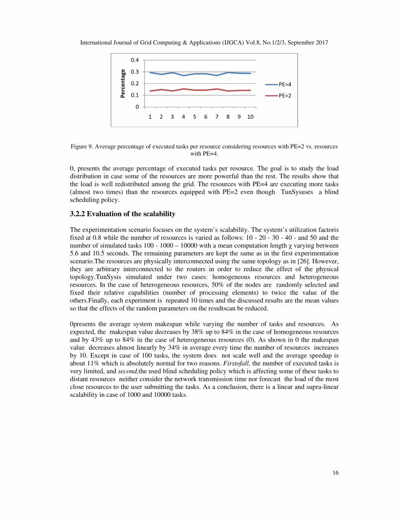
Figure 9. Average percentage of executed tasks per resource considering resources with PE=2 vs. resources

with PE=4.

0, presents the average percentage of executed tasks per resource. The goal is to study the load

distribution in case some of the resources are more powerful than the rest. The results show that

the load is well redistributed among the grid. The resources with PE=4 are executing more tasks

(almost two times) than the resources equipped with PE=2 even though TunSysuses a blind

scheduling policy.

3.2.2 Evaluation of the scalability The experimentation scenario focuses on the system’s scalability. The system’s utilization factoris

fixed at 0.8 while the number of resources is varied as follows: 10 - 20 - 30 - 40 - and 50 and the

number of simulated tasks 100 - 1000 – 10000 with a mean computation length χ varying between

5.6 and 10.5 seconds. The remaining parameters are kept the same as in the first experimentation

scenario.The resources are physically interconnected using the same topology as in [26]. However,

they are arbitrary interconnected to the routers in order to reduce the effect of the physical

topology.TunSysis simulated under two cases: homogeneous resources and heterogeneous

resources. In the case of heterogeneous resources, 50% of the nodes are randomly selected and

fixed their relative capabilities (number of processing elements) to twice the value of the

others.Finally, each experiment is repeated 10 times and the discussed results are the mean values

so that the effects of the random parameters on the resultscan be reduced.

0presents the average system makespan while varying the number of tasks and resources. As

expected, the makespan value decreases by 38% up to 84% in the case of homogeneous resources

and by 43% up to 84% in the case of heterogeneous resources (0). As shown in 0 the makespan

value decreases almost linearly by 34% in average every time the number of resources increases

by 10. Except in case of 100 tasks, the system does not scale well and the average speedup is

about 11% which is absolutely normal for two reasons. Firstofall, the number of executed tasks is

very limited, and second,the used blind scheduling policy which is affecting some of these tasks to

distant resources neither consider the network transmission time nor forecast the load of the most

close resources to the user submitting the tasks. As a conclusion, there is a linear and supra-linear

scalability in case of 1000 and 10000 tasks.

0

0.1

0.2

0.3

0.4

1 2 3 4 5 6 7 8 9 10P

erc

en

tag

e

PE=4

PE=2


Figure 10. Average makespan using 100, 1000, and 10000 tasks, 10

) vs. heterogeneous (

Figure 11.System speedup in case of 100,

1000, and 10000 tasks running under 10 and

50 resources.

3.2.3 Load balancing performance In order to study the load balancing performance of

focuses on the percentage of executed tasks per resource. As expected, the system load is better

distributed in case of homogeneous reso

resource as shown in 0and 0 In addition, every time the number of resources is increased by 10, the

load balancing is improved especially when the system

can lead to conclude that TunSys

heterogeneous resourcesneeds to

0

20

40

60

80

100

120

10 20 30 40 50

38%

82%84%

43%

81%

0%

10%

20%

30%

40%

50%

60%

70%

80%

90%

100 1000 10000

homogeneous heterogeneous


Average makespan using 100, 1000, and 10000 tasks, 10-50 resources, and homogenous (

) vs. heterogeneous ( ) resources.

System speedup in case of 100,

1000, and 10000 tasks running under 10 and

Figure 12.Average system speedup variation using 10,

20, 30, 40, and 50 resources.

balancing performance

In order to study the load balancing performance of TunSys, which is the main goal,

on the percentage of executed tasks per resource. As expected, the system load is better

distributed in case of homogeneous resources when considering the number of executed tasks per

In addition, every time the number of resources is increased by 10, the

load balancing is improved especially when the system executes bigger number of tasks (

TunSys scales well.However how the system reacts

to be verified.

0

200

400

600

800

1000

1200

10 20 30 40 50

0

2000

4000

6000

8000

10000

12000

10 20 30 40

84%84%

10000

heterogeneous

-10.00%

0.00%

10.00%

20.00%

30.00%

40.00%

50.00%

60.00%

20 30 40

100 heterogeneous 100 homogeneous




17

and homogenous (

Average system speedup variation using 10,

main goal, this section

on the percentage of executed tasks per resource. As expected, the system load is better

urces when considering the number of executed tasks per

In addition, every time the number of resources is increased by 10, the

bigger number of tasks (0). This

reacts in case of

40 50

50

100 homogeneous

1000 homogeneous

10000 homogeneous


Figure 13. Mean square deviation of the

percentage of executed tasks per resource in case

of homogeneous resources.

Figure 15. Mean square deviation of the percentage of

) vs. heterogeneous (

Figure .15.Average percentage of executed tasks per resourceconsidering resources with PE=2 (

The 0, presents the average percentage of executed tasks per resource. It compares the load

distribution between most powerful resources (PE=4) and

results show that the load distribution is considering the resource performance represented by

0

0.01

0.02

0.03

0.04

0.05

0.06

0.07

10 20 30 40

0

0.005

0.01

0.015

0.02

0.025

0.03

0.035

0.04

0.045

10 20 30 40 50

100 tasks

0

0.02

0.04

0.06

0.08

0.1

0.12

0.14

0.16

10 20 30 40 50


Mean square deviation of the

percentage of executed tasks per resource in case

of homogeneous resources.

Figure 14 Mean square deviation of the percentage

of executed tasks per resource in case of

heterogeneous resources.

Mean square deviation of the percentage of executed tasks per resource in case of homogenous (

) vs. heterogeneous ( ) resources with 100, 1000, and 10000 tasks.

Average percentage of executed tasks per resourceconsidering resources with PE=2 (

resources with PE=4 ( ) .

, presents the average percentage of executed tasks per resource. It compares the load

distribution between most powerful resources (PE=4) and less powerful resources (PE=2). The

results show that the load distribution is considering the resource performance represented by

50

0

0.01

0.02

0.03

0.04

0.05

0.06

0.07

0.08

10 20 30 40 50

0

0.01

0.02

0.03

0.04

0.05

0.06

0.07

0.08

10 20 30 40 50

1000 tasks

0

0.01

0.02

0.03

0.04

0.05

0.06

0.07

0.08

10 20 30 40

10000 tasks

0

0.02

0.04

0.06

0.08

0.1

0.12

0.14

0.16

0.18

10 20 30 40 50

0

0.02

0.04

0.06

0.08

0.1

0.12

0.14

0.16

0.18

10 20 30


18

Mean square deviation of the percentage

of executed tasks per resource in case of

executed tasks per resource in case of homogenous (

) resources with 100, 1000, and 10000 tasks.

Average percentage of executed tasks per resourceconsidering resources with PE=2 ( ) vs.

, presents the average percentage of executed tasks per resource. It compares the load

less powerful resources (PE=2). The

results show that the load distribution is considering the resource performance represented by the

100

1000

10000

40 50

40 50


19

number of processing elements (PE). The most powerful resources are executing more tasks (more

than the double especially in case of 10 nodes) except in case of 100 tasks which is due to the

limited number of tasks and the blind scheduling policy TunSysuses.

4. CONCLUSION In this work, a topology-aware load balancing method for grid computing systems is proposed.

Based on a polyhedron logical model with a sphere-like structure, the proposed method ensures a

local neighborhood load balancing strategy using a combination of a local and a global thresholds.

The proposed load balancing method is implemented and evaluated within a simple blind

scheduling strategy, since the load balancing problem is the aim of this work. GridSim simulator

isused for experimentalcomparison between TunSysand FCFS, DGA, and HGA through the

makespan and mean square deviation metrics.

The comparative evaluation of TunSys with FCFS, DGA and HGA shows encouraging results.In

fact, the system performance (measured through makespan) shows that TunSys outperforms FCFS,

DGA, and in most cases HGA. In addition, it shows an excellent system scalability that can reach

linear and supra-linear levels in case of 1000 and 10000 tasks. Furthermore, TunSys shows good

load balancing performance in terms of system stability by taking advantage of resource

heterogeneity, and the scalability of its load balancing approach.

Currently, the goal is to optimize the load balancing solution by integrating a better scheduling

policy. In addition, TunSyswill be compared to other more recent works involving different logical

models like star, tree, and peer-to-peer.

REFERENCES [1] R. Buyya and S. Venugopal, “A Gentle Introduction to Grid Computing and Technologies,” CSI

Commun., vol. 2, no. July, pp. 1–19, 2005.

[2] Y. Huang, N. Bessis, P. Norrington, P. Kuonen, and B. Hirsbrunner, “Exploring decentralized

dynamic scheduling for grids and clouds using the community-aware scheduling algorithm,” Futur.

Gener. Comput. Syst., vol. 29, no. 1, pp. 402–415, Jan. 2013.

[3] K. Yan, S. Wang, S. Wang, and C. Chang, “Towards a hybrid load balancing policy in grid

computing system,” Expert Syst. Appl., vol. 36, no. 10, pp. 12054–12064, 2009.

[4] R. Buyya, S. Chapin, and D. DiNucci, “Architectural models for resource management in the grid,”

Grid Comput. 2000, pp. 18–35, 2000.

[5] J. Cao, D. P. Spooner, S. a. Jarvis, G. R. Nudd, and S. Augustin, “Grid load balancing using

intelligent agents,” Futur. Gener. Comput. Syst., vol. 21, no. 1, pp. 135–149, Jan. 2005.

[6] Y. Li, Y. Yang, M. Ma, and L. Zhou, “A hybrid load balancing strategy of sequential tasks for grid

computing environments,” Futur. Gener. Comput. Syst., vol. 25, no. 8, pp. 819–828, Sep. 2009.

[7] A. Zomaya and Y. Teh, “Observations on using genetic algorithms for dynamic load-balancing,”

IEEE Trans. Parallel Distrib. Syst., vol. 12, no. 9, pp. 899–911, 2001.

[8] L. Bai, Y. L. Hu, S. Y. Lao, and W. M. Zhang, “Task scheduling with load balancing using

multiple ant colonies optimization in grid computing,” in Proceedings - 2010 6th International

Conference on Natural Computation, ICNC 2010, 2010, vol. 5, pp. 2715–2719.

[9] F. Xhafa and A. Abraham, “Computational models and heuristic methods for Grid scheduling

problems,” Futur. Gener. Comput. Syst., vol. 26, no. 4, pp. 608–621, Apr. 2010.

[10] J. C. Patni, M. S. Aswal, A. Agarwal, and P. Rastogi, “A Dynamic and Optimal Approach of Load

Balancing in Heterogeneous Grid Computing Environment,” in Emerging ICT for Bridging the

Future-Proceedings of the 49th Annual Convention of the Computer Society of India CSI, 2015,

vol. 2, pp. 447–455.

[11] K. Q. Yan, S. C. Wang, C. P. Chang, and J. S. Lin, “A hybrid load balancing policy underlying grid

computing environment,” Comput. Stand. Interfaces, vol. 29, no. 2, pp. 161–173, Feb. 2007.

[12] N. J. Kansal and I. Chana, “Cloud Load Balancing Techniques : A Step Towards Green

Computing,” IJCSI Int. J. Comput. Sci. Issues, vol. 9, no. 1, pp. 238–246, 2012.


20

[13] G. Terzopoulos and H. Karatza, “Energy-efficient real-time heterogeneous cluster scheduling with

node replacement due to failures,” J. Supercomput., vol. 68, no. 2, pp. 867–889, Dec. 2013.

[14] H. Barkallah, M. Gzara, and H. Ben Abdallah, “A fully distributed Grid meta scheduling method

for non dedicated resources,” in International Conference on Parallel and Distributed Processing

with Applications (ICPDPA’2014), IEEE WCCAIS’2014 Congress, 2014, no. 1, pp. 1–6.

[15] B. Yagoubi, “Load Balancing Strategy in Grid Environment,” J. Inf. Technol. Appl., vol. 1, no. 4,

pp. 285–296, 2007.

[16] M. S. B. Qureshi et al., “Survey on Grid Resource Allocation Mechanisms,” J. Grid Comput., vol.

12, no. 2, pp. 399–441, Apr. 2014.

[17] Y. Zhu and L. M Ni, “A survey on grid scheduling systems, Technical Report

SJTU_CS_TR_200309001,” 2013.

[18] J. Cao, “Self-organizing agents for grid load balancing,” in Proceedings of the 5th IEEE/ACM

International Workshop on Grid Computing, 2004, no. November, pp. 388–395.

[19] M. A. Salehi and H. Deldari, “Grid Load Balancing using an Echo System of Intelligent Ants.,” in

Parallel and Distributed Computing and Networks, 2006, pp. 47–52.

[20] M. A. Salehi, “Balancing Load in a Computational Grid Applying Adaptive , Intelligent Colonies

of Ants,” Informatica, vol. 33, no. 2, pp. 327–335, 2008.

[21] D. P. Spooner, S. a. Jarvis, J. Cao, S. Saini, and G. R. Nudd, “Local grid scheduling techniques

using performance prediction,” IEE Proc. - Comput. Digit. Tech., vol. 150, no. 2, p. 87, 2003.

[22] R. Subrata, A. Y. Zomaya, and B. Landfeldt, “Artificial life techniques for load balancing in

computational grids,” J. Comput. Syst. Sci., vol. 73, no. 8, pp. 1176–1190, 2007.

[23] L. He, S. A. Jarvis, D. Bacigalupo, D. P. Spooner, and G. R. Nudd, “Performance-Aware Load

Balancing for Multiclusters,” Parallel Distrib. Process. Appl. Second Int. ISPA 2004, vol. 3358, pp.

635–647, 2004.

[24] B. Yagoubi and Y. Slimani, “Dynamic Load Balancing Strategy for Grid Computing,” Trans. Eng.

Comput. Technol., vol. 13, pp. 260–265, 2006.

[25] K. Kandalla, H. Subramoni, A. Vishnu, and D. K. Panda, “Designing topology-aware collective

communication algorithms for large scale InfiniBand clusters: Case studies with Scatter and

Gather,” 2010 IEEE Int. Symp. Parallel Distrib. Process. Work. Phd Forum, pp. 1–8, Apr. 2010.

[26] W.-C. Yeh and S.-C. Wei, “Economic-based resource allocation for reliable Grid-computing

service based on Grid Bank,” Futur. Gener. Comput. Syst., vol. 28, no. 7, pp. 989–1002, Jul. 2012.

[27] M. Heidt, T. D, K. D, and B. Freisleben, “Omnivore: Integration of Grid Meta-Scheduling and

Peer-to-Peer Technologies,” 2008 Eighth IEEE Int. Symp. Clust. Comput. Grid, pp. 316–323, May

2008.

[28] S. Rho, H. Chang, S. Kim, and Y. S. Lee, “An efficient peer-to-peer and distributed scheduling for

cloud and grid computing,” Peer-to-Peer Netw. Appl., Apr. 2014.

[29] R.-M. Chen and C.-M. Wang, “Project scheduling heuristics-based standard PSO for task-resource

assignment in heterogeneous grid,” in Abstract and Applied Analysis, 2011, vol. 2011.

[30] V. Lo, K. J. Windisch, W. Liu, and B. Nitzberg, “Noncontiguous processor allocation algorithms

for mesh-connected multicomputers,” Parallel Distrib. Syst. IEEE Trans., vol. 8, no. 7, pp. 712–

726, 1997.

[31] G. Levitin and Y.-S. Dai, “Optimal service task partition and distribution in grid system with star

topology,” Reliab. Eng. Syst. Saf., vol. 93, no. 1, pp. 152–159, Jan. 2008.

[32] M.-C. Lee, F.-Y. Leu, and Y. Chen, “PFRF: An adaptive data replication algorithm based on star-

topology data grids,” Futur. Gener. Comput. Syst., vol. 28, no. 7, pp. 1045–1057, Jul. 2012.

[33] C. Coti, T. Herault, and F. Cappello, “MPI applications on grids: A topology aware approach,”

Euro-Par 2009 Parallel Process. Lect. Notes Comput. Sci., vol. 5704, pp. 466–477, 2009.

[34] M. Swany and R. Wolski, “Building performance topologies for computational grids,” Int. J. High

Perform. Comput. Appl., vol. 18, no. 2, pp. 255–265, 2004.

[35] W. Gentzsch, “Grid Computing: A New Technology for the Advanced Web,” in Advanced

Environments, Tools, and Applications for Cluster Computing SE - 1, vol. 2326, D. Grigoras, A.

Nicolau, B. Toursel, and B. Folliot, Eds. Springer Berlin Heidelberg, 2002, pp. 1–15.

[36] N. Fujimoto and K. Hagihara, “A comparison among grid scheduling algorithms for independent

coarse-grained tasks,” 2004 Int. Symp. Appl. Internet Work. 2004 Work., pp. 674–680, 2004.

[37] P. E. GmbH, “Validations Manual 4.2,” 2012. [Online]. Available: http://www.theseus-fe.com/.

[38] Z. Spakovszky, “MIT course: Introduction to Engineering Heat Transfer,” 2012. .

[39] H. Barkallah, M. Gzara, and H. Ben Abdallah, “Dynamic and adaptive topology-aware load

balancing for Grids,” in FCST’2014, 2014.


21

[40] R. Subrata, A. Y. Zomaya, B. Landfeldt, and S. Member, “Game-Theoretic Approach for Load

Balancing in Computational Grids,” IEEE Trans. Parallel Distrib. Syst., vol. 19, no. 1, pp. 66–76,

2008.

[41] M. A. Salehi, H. T. Yazdi, and M. R. A. Toutoonchi, “An optimal job selection method in load

balancing algorithms of economical grids,” in Innovations and Advanced Techniques in Systems,

Computing Sciences and Software Engineering, 2008, pp. 362–365.

[42] R. Buyya and M. Murshed, “GridSim: a toolkit for the modeling and simulation of distributed

resource management and scheduling for Grid computing,” Concurr. Comput. Pract. Exp., vol. 14,

no. 13–15, pp. 1175–1220, Nov. 2002.

[43] L. Kleinrock, Queueing Systems, Volume I: Theory. New York: Wiley Interscience, 1975.

Authors B. Haitham received a master degree in Computer Science and

multimedia from the University of Sfax, Tunisia. Currently, he is a Ph.D.

student and a member of the Multimedia, Information systems and

Advanced Computing Laboratory (Mir@cl), University of Sfax. His

research interests include grid and cloud computing, scheduling and load

balancing optimization.

M. Gzara received a PhD in automatic and industrial computing from the

University of Lille 1, France. She is currently an Associate Professor in

Computer Science at the Higher School of Computer Science and

Mathematics of Monastir, University of Monastir, Tunisia. She is a

member of the Multimedia, Information systems and Advanced

Computing Laboratory (Mir@cl), University of Sfax. Her research

interests include data mining techniques, Optimization, Parallelization,

Distributed Compuattion and Information Retrieval.

H. Ben-Abdallah received a BS in Computer Science and BS in

Mathematics from the University of Minnesota, MPLS, MN, a MSE and

PhD in Computer and Information Science from the University of

Pennsylvania, Philadelphia, PA. She worked at University of Sfax,

Tunisia from 1997 until 2013. She is now full professor at the Faculty of

Computing and Information Technology, King Abdulaziz University,

Jeddah, Kingdom of Saudi Arabia. She is a member of the Multimedia,

Information systems and Advanced Computing Laboratory (Mir@cl),

University of Sfax. Her research interests include software design quality,

reuse techniques in software and business process modeling.

topology aware load balancing for gridsaircconline.com/ijgca/v8n3/8317ijgca01.pdf · 2017-09-30 ·...

Documents