topology control in homogeneous wireless sensor networks

Topology Control

in Homogeneous Wireless Sensor Networks

using K-Means Clustering

Chinmaya Gautam

Department of Computer Science and EngineeringNational Institute of Technology RourkelaRourkela-769 008, Orissa, India

Topology Control

in Homogeneous Wireless Sensor Network

using K-Means Clustering

Thesis submitted in

May 2013

to the department of

Computer Science and Engineering

of

National Institute of Technology Rourkela

in partial fulfillment of the requirements

for the degree of

Bachelor of Technology

in

Computer Science and Engineering

by

Chinmaya Gautam

[Roll: 109CS0322]

under the guidance of

Prof. Bibhudatta Sahoo

Department of Computer Science and EngineeringNational Institute of Technology Rourkela

Rourkela-769 008, Orissa, India

Department of Computer Science and EngineeringNational Institute of Technology RourkelaRourkela-769 008, Odisha, India.

Certificate

This is to certify that the work in the thesis entitled Topology Control in Homoge-

neous Wireless Sensor Networks using K-Means Clustering by Chinmaya

Gautam is carried out by him under my supervision and guidance in partial fulfill-

ment of the requirements for the award of the degree of Bachelor of Technology in the

department of Computer Science and Engineering, National Institute of Technology

Rourkela.

Place: NIT Rourkela Bibhudatta SahooDate: 10 May 2013 Professor, CSE Department

NIT Rourkela, Odisha

Acknowledgment

No thesis is created entirely by an individual, many people have helped to create

this thesis and each of their contribution has been valuable. My deepest gratitude

goes to my thesis supervisor, Mr. Bibhudatta Sahoo, Asso. Professor, Department of

CSE, for his guidance, support, motivation and encouragement throughout the period

this work was carried out. His readiness for consultation at all times, his educative

comments, his concern and assistance even with practical things have been invaluable.

I would also like to thank all professors and lecturers, and members of the department

of Computer Science and Engineering for their generous help in various ways for the

completion of this thesis. A vote of thanks to my fellow students for their friendly

co-operation.

Chinmaya Gautam

Abstract

A wireless sensor network consists of many wireless nodes forming a network which

are used to monitor certain physical or environmental conditions, such as humidity,

temperature, sound etc. Some of the popular applications of sensor network are area

monitoring, environment monitoring (such as pollution monitoring), and industrial

and machine health monitoring, waste water monitoring and military surveillance.

Topology control in WSNs is a technique of defining the connections between nodes

in order to reduce the interference between them, save energy and extend network

lifetime.

The Objective of my Thesis is to Maximize the network lifetime. The algorithm

proposed is a modification to the CLTC framework: first we form clusters of nodes

using K-Means, in second phase we do intra-cluster topology control using Relative

Neighborhood Graph, and in third phase we do inter-cluster topology control ensuring

connectivity. The simulations were carried out using Omnet++ as a simulator and

Node Power Depletion and Node Lifetime as parameters.

Contents

Certificate ii

Acknowledgement iii

Abstract iv

List of Abbreviations vii

List of Figures viii

List of Algorithms ix

1 Introduction 1

1.1 Topology Control in Wireless Sensor Networks . . . . . . . . . . . . . 2

1.2 Literature Review . . . . . . . . . . . . . . . . . . . . . . . . . . . . . 2

1.2.1 Effects of Power Control on Connectivity . . . . . . . . . . . . 2

1.2.2 Relative Neighborhood Graph (RNG) . . . . . . . . . . . . . . 3

1.2.3 Gabriel Graph(GG) . . . . . . . . . . . . . . . . . . . . . . . . 4

1.2.4 CLTC . . . . . . . . . . . . . . . . . . . . . . . . . . . . . . . 5

1.3 Motivation . . . . . . . . . . . . . . . . . . . . . . . . . . . . . . . . . 6

1.4 Objective . . . . . . . . . . . . . . . . . . . . . . . . . . . . . . . . . 6

1.5 Outline of thesis . . . . . . . . . . . . . . . . . . . . . . . . . . . . . . 7

2 Topology Control 8

2.1 Introduction . . . . . . . . . . . . . . . . . . . . . . . . . . . . . . . . 8

2.2 Metrics for WSN . . . . . . . . . . . . . . . . . . . . . . . . . . . . . 8

2.3 Options for Topology Control . . . . . . . . . . . . . . . . . . . . . . 10

2.4 Taxonomy of Topology Control Problem . . . . . . . . . . . . . . . . 11

2.4.1 Homogeneous approach . . . . . . . . . . . . . . . . . . . . . . 11

v

2.4.2 Heterogeneous approach . . . . . . . . . . . . . . . . . . . . . 12

2.5 Network and Communication Model . . . . . . . . . . . . . . . . . . 12

2.6 Path Loss Model . . . . . . . . . . . . . . . . . . . . . . . . . . . . . 13

2.7 Conclusion . . . . . . . . . . . . . . . . . . . . . . . . . . . . . . . . . 14

3 Implementing CLTC using k-means 15

3.1 Introduction . . . . . . . . . . . . . . . . . . . . . . . . . . . . . . . . 15

3.2 Phase I: Cluster Formation . . . . . . . . . . . . . . . . . . . . . . . . 17

3.3 Phase II: Intra Cluster TC . . . . . . . . . . . . . . . . . . . . . . . . 20

3.4 Phase III: Inter Cluster TC . . . . . . . . . . . . . . . . . . . . . . . 20

3.5 Conclusion . . . . . . . . . . . . . . . . . . . . . . . . . . . . . . . . . 22

4 Simulation and Results 25

4.1 Simulation . . . . . . . . . . . . . . . . . . . . . . . . . . . . . . . . . 25

4.2 Results . . . . . . . . . . . . . . . . . . . . . . . . . . . . . . . . . . . 27

4.2.1 Average Transmission Power vs. Number of Nodes . . . . . . 27

4.2.2 Node Power Depletion . . . . . . . . . . . . . . . . . . . . . . 28

4.2.3 Node Lifetime . . . . . . . . . . . . . . . . . . . . . . . . . . . 28

4.3 Analysis . . . . . . . . . . . . . . . . . . . . . . . . . . . . . . . . . . 28

4.4 Conclusion . . . . . . . . . . . . . . . . . . . . . . . . . . . . . . . . . 32

5 Conclusions and Future Work 33

Bibliography 34

vi

List of Abbreviations

WSN Wireless Sensor Network

CLTC Cluster Based Topology Control

TC Topology Control

RNG Relative Neighborhood Graph

GG Gabriel Graph

NPD Node Power Depletion

NL Node Lifetime

List of Figures

1.1 Effect of power control on connectivity: number of connected nodes vs

transmission range . . . . . . . . . . . . . . . . . . . . . . . . . . . . 3

1.2 Relative Neighborhood Graph . . . . . . . . . . . . . . . . . . . . . . 4

1.3 Gabriel Graph . . . . . . . . . . . . . . . . . . . . . . . . . . . . . . 5

2.1 taxonomy of topology control problem . . . . . . . . . . . . . . . . . 11

3.1 A network without any Topology Control implementation . . . . . . 16

3.2 Clustering of 100 nodes spread in a 1000 x 1000 area . . . . . . . . . 19

3.3 Intra Cluster TC of 100 nodes spread in a 1000 x 1000 area . . . . . . 21

3.4 Inter Cluster TC of 100 nodes spread in a 1000 x 1000 area . . . . . . 23

4.1 Simulating a 100 node WSN ins Omnet++ . . . . . . . . . . . . . . 26

4.2 Simulation results of 100 node WSN in Omnet++ . . . . . . . . . . . 27

4.3 plot of average transmission power. vs number of nodes . . . . . . . . 28

4.4 node power depletion vs. time for network with no topology control . 29

4.5 node power depletion vs. time for network with no k-means cluster

based topology control . . . . . . . . . . . . . . . . . . . . . . . . . . 29

4.6 node power depletion vs. time for network with CLTC:k-means based

topology control . . . . . . . . . . . . . . . . . . . . . . . . . . . . . . 30

4.7 node life time of 100 nodes for network with no topology control . . . 30

4.8 node life time of 100 nodes for network with k-means cluster based


4.9 node life time of 100 nodes for network with CLTC:k-means based


viii

List of Algorithms

1 Clustering nodes for Phase I . . . . . . . . . . . . . . . . . . . . . . . 17

2 Finding new mean nodes for K-Means Clustering . . . . . . . . . . . 18

3 Forming Intra Cluster Topology using RNG for Phase II . . . . . . . 22

4 inter cluster topology control for phase III . . . . . . . . . . . . . . . 24

ix

Chapter 1

Introduction

A sensor network is a network of sensor nodes which are capable of sensing, comput-

ing and communicating elements and it gives an administrator the ability to measure,

observe and react to events and phenomenon in a specific environment.

Sensor networks are typically applied to the area of data collection, monitoring surveil-

lance, military applications, and medical telemetry.

Recent advancement in wireless communications and electronics has enabled the de-

velopment of low-cost, low-power, multi-functional miniature devices for use in remote

sensing applications. The combination of these factors has improved the viability of

utilizing a sensor network consisting of a large number of intelligent sensors, enabling

the collection, processing analysis and dissemination of valuable information gathered

in a variety of environments. Instead of sending the raw data to the nodes responsible

for the fusion, they use their processing abilities to locally carry out simple computa-

tions and transmit only the required and partially processed data.

Sensor networks are predominantly data-centric rather than address-centric. So sensed

data are directed to an area containing a number of sensors rather than particular

sensor addresses. Aggregation of data increases the level of accuracy and reduces data

redundancy. A network hierarchy and clustering of sensor nodes allows for network

scalability, robustness, efficient resource utilization and lower power consumption.

1

1.1 Topology Control in Wireless Sensor Networks Introduction

1.1 Topology Control in Wireless Sensor Networks

Topology control can be defined as the process of configuring or reconfiguring a net-

works topology through tunable parameters after deployment. There are 3 mazor

tunable parameters for topology control in WSN are:

• Node mobility: In WSNs consisting of mobile nodes, such as robotics sensor

networks, both coverage and connectivity can be adapted by moving the nodes

accordingly.

• Transmission power control: In WSNs with static nodes, if the deployment

density is already sufficient to generate the required level of coverage, the con-

nectivity properties of the network can be adjusted by tuning the transmission

power of constituent nodes.

• Sleep scheduling: In large scale static WSNs deployed at a high density, i.e.

over deployed. In this case the appropriate topology control mechanism that

provides energy efficiency and extends network lifetime is to turn off nodes that

are redundant.

Topology control problem has been proved to be an NP-Complete problem[1]

1.2 Literature Review

1.2.1 Effects of Power Control on Connectivity

On varrying the transmission power of the nodes, it’s number of neighbors can be

varried. Assuming the disk graph model, we study the effect of varying the transmis-

sion power, and hence he transmission range on the size of the maximum connected

component in randomly deployed wireless sensor network. A flat network topology is

assumed.

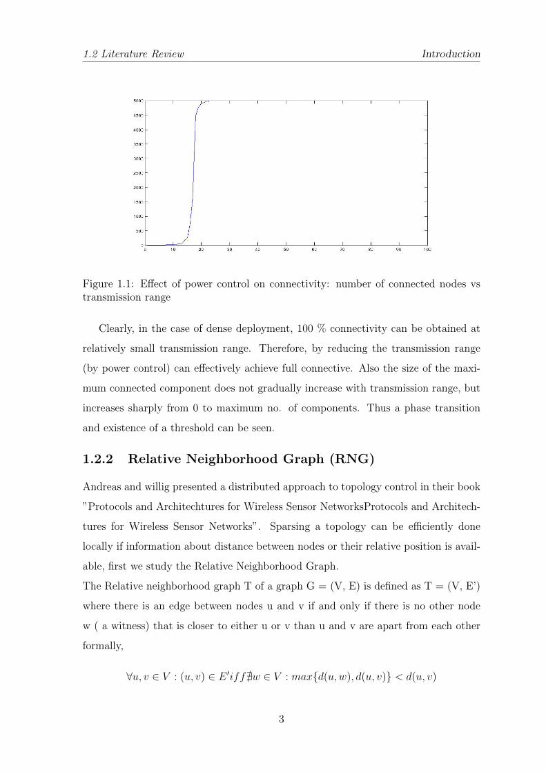
On simulating a randomly deployed sensor network, with 5000 nodes in a 1500 x

1500 unit are with maximum transmission range of 100 units, the following plot was

obtained:

2

1.2 Literature Review Introduction

Figure 1.1: Effect of power control on connectivity: number of connected nodes vstransmission range

Clearly, in the case of dense deployment, 100 % connectivity can be obtained at

relatively small transmission range. Therefore, by reducing the transmission range

(by power control) can effectively achieve full connective. Also the size of the maxi-

mum connected component does not gradually increase with transmission range, but

increases sharply from 0 to maximum no. of components. Thus a phase transition

and existence of a threshold can be seen.

1.2.2 Relative Neighborhood Graph (RNG)

Andreas and willig presented a distributed approach to topology control in their book

”Protocols and Architechtures for Wireless Sensor NetworksProtocols and Architech-

tures for Wireless Sensor Networks”. Sparsing a topology can be efficiently done

locally if information about distance between nodes or their relative position is avail-

able, first we study the Relative Neighborhood Graph.

The Relative neighborhood graph T of a graph G = (V, E) is defined as T = (V, E’)

where there is an edge between nodes u and v if and only if there is no other node

w ( a witness) that is closer to either u or v than u and v are apart from each other

formally,

∀u, v ∈ V : (u, v) ∈ E ′iff@w ∈ V : max{d(u,w), d(u, v)} < d(u, v)

3


Figure 1.2: Relative Neighborhood Graph

where d (u, v) is the Euclidean distance.between two nodes.

But a this algorithm does not guarentee a strong connectivity.

1.2.3 Gabriel Graph(GG)

Another algorithm presented by andreas and willig was the gabriel graph for sparsing

the topology. The Gabriel Graph (GG) is defined similarly to the RNG; the formal

definition for it’s edges is

∀u, v ∈ V : (u, v) ∈ E ′iff@w ∈ V : d2(u,w) + d2(v, w) < d2(u, v).

The nodes were randomly deployed in a 250 x 250 unit square area. Each node

having a transmission power of 100 units. Both RNG as well as GG sparse the

topology. In case of RNG, for some nodes which are only a few hops apart in the

original graph becomes very distant. Even though this algorithm has a stronger

connectivity than RNG, its quantitative value cannot be determined.

4


Figure 1.3: Gabriel Graph

1.2.4 CLTC

CLTC stands for Cluster Based Topology Control. It was proposed by Shen et. al.

It is a hybrid topology control framework that achieves both scalability and strong

connectivity. The framework proposes dividing the Topology configuration into three

phases:

• Cluster Formation: In the first phase clusters are formed from the nodes using

a suitable clustering algorithm

• Intra Cluster Topology Control: In the second phase a centralized topology

control algorithm is used to define the topology of each cluster as a sub-network.

• Inter Cluster Topology Control: In the third phase the clusters are connected

to each other to form the final topology of the network.

The authors present one implementation of this framework: CLTC-A which analyzes

the message complexity of the network. The energy of the network was not dealt with

5

1.3 Motivation Introduction

in this paper.

1.3 Motivation

Saving energy is a very critical issue in wireless sensor networks (WSNs) since sensor

nodes are typically powered by batteries with a limited capacity. Since the radio

transmission is the main cause of power consumption in a sensor node, transmis-

sion/reception of data should be limited as much as possible. In wireless sensor

networks, energy is considered a scarce resource:

• The sensor nodes are battery operated.

• Nodes and hence the wireless sensor network has a limited lifetime.

If transmission power is controlled, the network lifetime can be optimized.

1.4 Objective

In a Sensor Network Deployment, if the topology of the network is not controlled, all

nodes transmit data at their maximum energy and hence, the lifetime of the network

is considerably reduced. Many popular methods exist to modify the topology and

prolong the network lifetime, these include distributed topology control mechanisms,

centralized mechanisms and cluster based methods amongst others.

The Objective of my work is to maximize the network life time of a Wireless Sensor

Network. This can be achieved by minimizing the transmission power of nodes while

maintaining connectivity.

The idea is to minimize the average transmission power of nodes:

Eavg =

∑ni=1Ein

where,

Ei = transmission power of node i

n = number of nodes

Eavg = average transmission power

6

1.5 Outline of thesis Introduction

The overall energy of the network is given by[2]:

E(z, t) = lim|S|→0

1

|S|∑

sensori∈S

ei(t)

where,

z = location of the node,

t=time,

S = connected area in the network,

ei(t) = residual energy of node i at time t

1.5 Outline of thesis

In this chapter, we present the Topology Control Problem in Wireless Sensor Net-

works, The problem statement and objectives of our work are discussed briefly. The

organization of the rest of the thesis and a brief outline of the chapters in this thesis

are as given below.

Chapter 2:Topology Control

We discuss the topology control problem and present the various parameters used for

analysis of wireless sensor networks, and the options for topology control. We further

present taxonomy for the topology control problem.

Chapter 3:CLTC using K-Means

We present our implementation of the Cluster Based Topology Control Framework

using K-Means Clustering to minimize average transmission power.

Chapter 4: Simulation and Results

This chapter presents the simulations, results and analysis of the implementation of

CLTC:K-Means.

Chapter 5:Conclustion and Future Work

This chapter summarizes the thesis and presents the future directions for this work.

7

Chapter 2

Topology Control

2.1 Introduction

Topology control can be defined as the process of configuring or re-configuring a

network’s topology through tunable parameters after deployment.[3]

Let V denote the set of wireless sensor nodes and G(V,E) denote the subgraph on V

that contains all possible edges if each node transmits at its maximum transmission

power. The edge set E of G is constructed in such a manner that there is a directed

edge from u to v if and only if u can reach v using its maximum transmission power.

Graph G sets an upperbound on the maximum connectivity that a wireless network

can have. The topology control algorithm returns a topology T constructed from G,

i.e., T is a subgraph of G on V.[4]

A wireless sensor network should fulfill the following connectivity requirement:

For any pair of nodes u and v, if there is a path from u to v in G then there is also a

path from u to v in T.[4]

2.2 Metrics for WSN

Wireless environment are unreliable, with error rate high that introduce burst errors.

Various parameters that are used to measure the efficiency of wireless sensor networks

are[1]:

• Throughput: The throughput of the most important parameter to analyze the

performance of the network. It is the amount of data transmitted per unit time.

8

2.2 Metrics for WSN Topology Control

Throughput is measured in bits/sec. Throughput T in a network is given by:

T = d/t

where,

d = data transmitted in bits,

t = total time

• Packet delivery ratio: It is the ration of number of packets received to no.

of packets generated. Packet delivery ratio is given as:

Pdr =Nrecd

Ngen

where,

Pdr = packet delivary ratio,

Nrecd = number of packets received,

Ngen = number of packets generated

• Packet loss: It is the number of packets lost in transmission. Packet loss

is distinguished as one of the three main error types encountered in digital

communication. Packet loss is given by:

Ploss = Pgen − Precd

where,

Ploss = number of packets lost

• Bit error rate/bit error ratio: It is the number of received bits that have

been altered due to noise, interference and distortion, divided by total number

of transferred bits during a particular time interval. The bit error rate is given

by:

BER =1

2

√erfc(

EbN0

)

where,

BER = bit error ratio

9

2.3 Options for Topology Control Topology Control

erfc = error function

Eb = energy per bit

N0 = noise power

• Energy consumption: It is important parameter, as each sensor node has a

limited amount of energy, which depletes on re-transmission. The energy of a

network is given by[2]:

E(z, t) = lim|S|→0

1

|S|∑

sensori∈S

ei(t)

where,

z = location of the node,

t=time,

S = connected area in the network,

ei(t) = residual energy of node i at time t

2.3 Options for Topology Control

To compute a modified graph I out of a graph G representing the original network G,

a topology control algorithm has a few options:

The set of active nodes can be reduced (Vt ∈ V ), for example, by periodically switch-

ing off nodes with low energy reserves and activation other nodes instead, exploiting

redundant deployment in doing so.

The set of active links/the set of neighbors for a node can be controlled. Instead

of using all links in a network, some links can be disregarded and communication is

restricted to crucial links. When a flat network topology is desired (all nodes are

considered equal), the set of neighbors of a node can be reduced by simply not com-

municating with some neighbors. There are several possible approaches to choose

neighbors, but one that is obviously promising for a WSN is to limit the reach of a

node’s transmission typically by power control, but also by using adaptive modula-

tion (using faster modulation is only possible over shorter distance) and using the

improved energy efficiency when communicating only with nearby neighbors.

10

2.4 Taxonomy of Topology Control Problem Topology Control

Figure 2.1: taxonomy of topology control problem

Active links/neighbors can also be rearranged in a hierarchical network topology where

some nodes assume special roles. One example is to select some nodes as a ”back-

bone” (or a ”spine”) for the network and to only use the links within this backbone

and direct links from other nodes to backbone.[5]

2.4 Taxonomy of Topology Control Problem

The topology control problem can be broadly divided into two types based on the

type of nodes deployed [6]:

• homogeneous approach

• heterogeneous approach

We discuss both types of approaches in subsequent subsections.

2.4.1 Homogeneous approach

In case of homogeneous approach, nodes are assumed to use the same transmitting

range, and the topology control problem reduces to the one of determining the mini-

mum value of r (range) such that a certain network wide property is satisfied ( the

Critical Transmitting Range).

Our work follows the homogeneous approach to topology control.

11

2.5 Network and Communication Model Topology Control

2.4.2 Heterogeneous approach

In this case, nodes are allowed to choose different transmitting ranges (provided they

do not exceed the maximum range).

Nonhomogeneous topology control is classified into three categories, depending on

the type of information that is used to compute the topology. In location based ap-

proaches, exact node positions are known.

This information is either used by a centralized authority to compute a set of trans-

mitting range assignments which optimize a certain measure ( this is the case of the

Range Assignment problem and its variants), or it is exchanged between nodes and

used to compute an almost optimal topology in a fully distributed manner / this is the

case for protocols used for building energy efficient topologies for unicast or broadcast

communication).

In direction based approaches, it is assumed that nodes do not know their position,

but they can estimate the relative direction of each of their neighbors. Finally in

neighbor-based techniques, nodes are assumed to know only the ID of their neigh-

bors and are able to order them according to some criterion (E.g. distance, or link

quality).[7]

2.5 Network and Communication Model

We present the network and communication model used for the CLTC framework as

initially proposed by shen et. al:

M= (N, L) is a mulithop wireless network where N = {m1,m2,m3, ,mn} is a set of

nodes and L is a one-to-one mapping from N to planar coordinates. Each node is able

to obtain its coordinate by some means (e.g. GPS). Further each node u is able to

adjust its transmission power level pu within the range 0 ≤ pu ≤ Pmax, where Pmax

is the maximum transmission power (we assume this value is the same for all nodes).

For a node u to successfullycommunicate with another node v, the signal received

at v must exceed the receive sensitivity S. Recall that signals lose their power as a

function of distance when propagating through a communication medium. Here, the

path loss propagation function is (in dB) γ(lu, lv), where the signal travels from u to

12

2.6 Path Loss Model Topology Control

v andlu, lv are the coordinates of nodes u and v, respectively.

In order to guarantee a successful reception at v, it must be that pu ≥ S + γ(lu, lv).

We assume that γ is monotonically increasing function of the distance between u and

v and the function λ(d) maps the distance d to the minimum. Transmission power

required for successful communication at the distance. Thus, a node u is able to

determine its minimum transmission power to reach v from λ(d(lu, lv)) = S+γ(lu, lv).

Given this framework, a network M= (N, L) can be represented by an undirected

graph G= (V, E), whereV = u1, u2, , un and vertex u, corresponding to node mi, in

M. There is an edge in G between a pair of vertices if their corresponding distance in

M enables a successful communication. That is,

E = {(ui, uj)}, ui, uj ∈ V

and

S + γ(mi,mj) ≤ Pmax

[6]

2.6 Path Loss Model

When nodes communicate, they loose their energy. The power required to communi-

cate to a node is related to the distance of communication using path loss models.

We use the path loss model presented by Ebenezer et al. which is presented here:

Two nodes, seperated by a distance ’x’ can communicate with each other only if the

strength of the signal received is greater than the receiver’s sensitivity threshold. As

the signal propagates through the channel, its power density is reduced. The relation

between the power Px required to communicate at a distance x is given by:

The energy Px required to communicate at a destination x is given by

Px = P0(x

d0)α

where P0 is the energy required to communicate at a distance d0 [8].

13

2.7 Conclusion Topology Control

2.7 Conclusion

In this chapter we presented the topology control problem as an optimization problem.

We discussed the various parameters for the study of topology control problem, its

classification and various options for topology control. We also saw the network and

communication model and the path loss model for WSN.

14

Chapter 3

Implementing CLTC using k-means

3.1 Introduction

CLTC stands for Cluster Based Topology Control. It was proposed by Shen et.

al. It is a hybrid topology control framework that achieves both scalability and

strong connectivity. By varying the algorithms utilized in each of the three phases

of the framework, a variety of optimization objectives and topological properties can

be achieved. In this thesis, we present the implementation of CLTC framework for

minimization of transmission power using k-means clustering.

The framework divides the TC problem into 3-phases:

• Cluster formation

• Intra Cluster topology Control

• Inter Cluster topology Control

We divide the construction of the network topology into the three aforementioned

phases.

In The first Phase, we use k-means for forming k distinct clusters out of the total

N nodes in the network. Moreover, a cluster head is selected for each cluster. We

assume in this phase that all nodes are transmitting at their maximum power and

only connections possible are those within the cluster.

Once clusters have been formed, each cluster modifies its topology using the relative

neighborhood graph to further optimize the transmission power. These new trans-

mission powers are stored with the nodes. The nodes do not start transmitting data

15

3.1 Introduction Implementing CLTC using k-means

Figure 3.1: A network without any Topology Control implementation

at this point of time.

In the third phase, all pairs of clusters ui, uj try to connect to each other if the maxi-

mum transmission range of the boundary nodes of ui can contact any boundary node

of uj . For all such successful connections, the transmission power of boundary nodes

are set to the maximum of its present transmission power and the new value required

to communicate with other clusters.

16

3.2 Phase I: Cluster Formation Implementing CLTC using k-means

3.2 Phase I: Cluster Formation

In the first phase, in a distributed fashion, clusters are formed and cluster heads are

selected. Note that the operations in the subsequent two phases are independent of the

specific clustering algorithm used in this phase. Any distributed clustering algorithm

that can form non-overlapping clusters and select cluster heads can be applied. We

use K-Means Clustering to form the clusters from the node deployed in the network

as follows:

At first we select K random nodes from the set of nodes N, these form the initial

set of cluster heads then for each node ui, we find the closest cluster (using Euclidian

Distance between nodes) head and label ui with the nodeID of this cluster head. Once

all nodes have been assigned a label, we find the centroid of each cluster and label

the node closest to the centroid as the new cluster head for the cluster. This process

is repeated for R ( = N/10) number of times, to form the clusters.

Algorithm 1 Clustering nodes for Phase I

for i=1 to N/10 doclusterHeads[i] = rand()%MAX NODES

end forfor i = 1 to 10 do

for j = 1 to N dominDist =∞for k = 1 to N/10 donewDist = distance(nodes[j], nodes[clusterHeads[j]])if newDist <minDist thenminDist = newDistnodes[j].label = k

end ifend for

end forclusterHeads = newMeans(nodes)

end for

The algorithm to find new means is preseneted further:

17


Algorithm 2 Finding new mean nodes for K-Means Clustering

for j=1 to K dototalx=0totaly=0entries=0for i=1 to N do

if nodes[i].label = j thentotalx = totalx+ nodes[i].xtotaly = totaly + nodes[i].yentries++

end ifend forclusterHeads[j].x = totalx/entriesclusterHeads[j].y = totaly/entries

end forfor j= 0 to K do

for i = 1 to N dominDist =∞if distance(nodes[i], clusterHeads[j] < minDist then

minDist = eucledianDistance(nodes[i], clusterHeads[j])nodes[i].label=clusterHeads[j]

end ifend for

end for

18


Figure 3.2: Clustering of 100 nodes spread in a 1000 x 1000 area

19

3.3 Phase II: Intra Cluster TC Implementing CLTC using k-means

3.3 Phase II: Intra Cluster TC

In Phase I, all the nodes have been partitioned into distinct clusters, in this phase we

modify the topology of each the network by considering each cluster as an isolated

sub-network.

The power assignments of the cluster members can be obtained by applying the al-

gorithm3 presented further.

The power assignments calculated in this phase will be distributed to the cluster

members. But, the cluster members will not yet begin transmitting at these powers.

Rather, it may be that these powers will be found to be inadequate as a result of

Phase 3 (the intercluster topology control phase). Hence, the final power assignments

for all nodes will be computed after Phase 3 is completed. Thus, during Phase 3,

all nodes will still utilize their full transmission power. Only after the completion of

Phase 3 will nodes start using their assigned transmission power.

We use the Relative Neighborhood Graph to obtain power assignments of various

nodes. RNG can effectively sparse a topology. In the Relative neighborhood graph T

of a graph G, there is an edge between nodes u and v if and only if there is no other

node w ( a witness) that is closer to either u or v than u and v are apart from each

other, thus RNG also guarantees a k-1 connectivity, so we can assume that all the

nodes within a cluster will be connected.

3.4 Phase III: Inter Cluster TC

In Phase II, the intra-cluster topology of the network is set, after this phase, all nodes

are connected within their clusters whereas nodes belonging to different clusters are

not connected.

In this phase, connectivity between adjacent clusters is considered. For all pairs of

clusters Ci, Cj, if the maximum transmission range of the boundary nodes of ui ∈ Cican contact any boundary node of uj ∈ Cj we form the connection (ui, uj).

For all such successful connections, the transmission power of boundary nodes are

set to the maximum of its present transmission power and the new value required to

20

3.4 Phase III: Inter Cluster TC Implementing CLTC using k-means

Figure 3.3: Intra Cluster TC of 100 nodes spread in a 1000 x 1000 area

21

3.5 Conclusion Implementing CLTC using k-means

Algorithm 3 Forming Intra Cluster Topology using RNG for Phase II

for i = 1 to K dofor j = 1 to size(clusters[i]) do

for k = j to size(clusters[i]) doformLink = 1for l = 1 to size(clusters[i]) do

if (max(distance(nodes[i],nodes[l]),distance(nodes[j],nodes[l]))¡distance(nodes[i],nodes[j]))then

formLink = 0end if

end forif formLink == 1 then

nodes[i].power = max(nodes[i].power, powerAssign-ment(distance(nodes[i],nodes[j]))nodes[j].power = max(nodes[j].power, powerAssign-ment(distance(nodes[i],nodes[j]))

end ifend for

end forend for

communicate with other clusters.

Now, we present the algorithm for the third phase :

3.5 Conclusion

In this chapter, we present the path loss model communication between nodes. This

chapter also shows the implementation of CLTC using k-means in three phases: the

cluster formation phase (in which k-means is used), the intra cluster topology con-

trol phase (in which relative neighborhood graph is used) and the final inter cluster

topology control phase.

22


Figure 3.4: Inter Cluster TC of 100 nodes spread in a 1000 x 1000 area

23


Algorithm 4 inter cluster topology control for phase III

for i = 1 to K dofor j = i to K do

for k = 1 to clusters[i] dofor l = 1 to clusters[j] do

if distance(nodes[k],nodes[l]) ¡ minDist) thenminDist = distance(nodes[k],nodes[l])node1 = knode2 = l

end ifend for

end forif powerAssignment(minDist) ¿ nodes[node1].power then

nodes[node1].power = powerAssignment(minDist)end ifif powerAssignment(minDist) ¿ nodes[node2].power then

nodes[node2].power = powerAssignment(minDist)end if

end forend for

24

Chapter 4

Simulation and Results

In this chapter we present the Simulation of the network, the output plots and its

analysis.

4.1 Simulation

For the Simulation of the Network, Omnet++ was used. OMNeT++ is an extensi-

ble, modular, component-based C++ simulation library and framework, primarily for

building network simulators. First, we create a simple module called ”node”. This

module contains all functionalities that the WSN nodes can carry out independently:

• Sensing: data is generated virtually by each node, this data acts as the sensed

data.

• Computation:The computation done on data can be specified for each node.

• Communication:The data is sent to other nodes by either specifying the out-

put port to be used or the target node id.

Then a network is created. We set the simulation area to 1000x1000 for this

network and initialize the network with 100 nodes of the simple module created earlier.

The topology of the network can be set in this network by specifying the connections

between nodes.

The network can now be simulated by running the project as a Omnet++ simulation.

All simulation data and logs are saved to a le which can be used later for analysis.

25

4.1 Simulation Simulation and Results

Figure 4.1: Simulating a 100 node WSN ins Omnet++

26

4.2 Results Simulation and Results

Figure 4.2: Simulation results of 100 node WSN in Omnet++

4.2 Results

The results collected from the simulation were plot to a graph. We study the varia-

tion average transmission power of nodes with the number of nodes in the network.

We simulate the network in a constant area (of 1000x1000 unit area) with constant

maximum transmission power of the nodes.

4.2.1 Average Transmission Power vs. Number of Nodes

The simulation if run 10 times for each value of number of nodes varying from 50 to

500 in intervals of 50 nodes and are averaged. The results obtained for networks with

• No topology control

• K-Means without CLTC

• K-Means with CLTC

are plot vs. the number of nodes.

27

4.3 Analysis Simulation and Results

Figure 4.3: plot of average transmission power. vs number of nodes

4.2.2 Node Power Depletion

The simulation is run for 100 nodes and the node power depletion is plot for networks

with no topology control, networks with k-means clustering and networks with CLTC

implementation of k-means.

4.2.3 Node Lifetime

The simulation is run for 100 nodes and the node lifetime is plot for networks with

no topology control, networks with k-means clustering and networks with CLTC im-

plementation of k-means.

4.3 Analysis

From the Simulation and the Results Obtained we conclude that:

• When no topology control is deployed and all nodes transmit at maximum

power, the average transmission power of nodes is a constant (with the value =

28


Figure 4.4: node power depletion vs. time for network with no topology control

Figure 4.5: node power depletion vs. time for network with no k-means cluster basedtopology control

29


Figure 4.6: node power depletion vs. time for network with CLTC:k-means basedtopology control

Figure 4.7: node life time of 100 nodes for network with no topology control

30


Figure 4.8: node life time of 100 nodes for network with k-means cluster basedtopology control

Figure 4.9: node life time of 100 nodes for network with CLTC:k-means based topol-ogy control

31

4.4 Conclusion Simulation and Results

maximum transmission power of the node)

• Simple K-Means shows a much lower average transmission power as compared

to networks with no topology control. Moreover, the average transmission power

in case of k-means decreases as the number of nodes in the network increases.

• When CLTC is used, the average transmission power of the nodes is lesser

than that of k-means, showing improvement. The transmission powers of nodes

decreases with the increasing number on node deployment.

4.4 Conclusion

In this chapter we presented the simulation of the WSN using Omnet++. We com-

pared the average transmission power of nodes vs. the number on nodes in case of

networks with no topology control, with k-means clustering based topology control

and with CLTC:k-means based topology control. We also analyzed the eect of the

proposed work on node power depletion and node lifetime as compared to simple

k-means or no topology control.

32

Chapter 5

Conclusions and Future Work

This thesis proposes modification to the CLTC framework so that it can be applied

to Wireless Sensor Networks when the network lifetime has to be optimized. In order

to do so, first of all we use a distributed approach in the second phase as compared to

the centralized approach initially presented. This assures that the power consumption

of cluster heads is minimized.

The second presentation in this thesis is the implementation of the framework to

minimize the node power consumption of nodes using k-means clustering, which is

a simple clustering method to deploy in WSNs. We also present the effects of this

implementation on node lifetime.

The following approaches can be taken up as future work related to this project:

• Study of Network Coverage using CLTC: When the transmission power of nodes

are changed, their transmission range changes, hence the network coverage is

affected. The study of Network Coverage when implementing CLTC can be

done.

• Effects of deploying other algorithms for intra-cluster topology control: We

used the Relative Neighborhood graph for intra-cluster topology control; other

sparsing algorithms can be implemented.

• Deployment of CLTC to Heterogeneous Networks: Our proposed work assumes

a homogeneous network, but CLTC can be deployed to heterogeneous models

as well.

33

Bibliography

[1] Hsiao Hwa Chen Konstantinidis Andreas, Yang Kun and Zhang Qingfu. Energy-aware topology

control for wireless sensor networks using manetic algorithms.

[2] Mehdi Kalantari and Mark Shayman. Energy efficient routing in wireless sensor networks. In

Proc. of Conference on Information Sciences and Systems. Citeseer, 2004.

[3] Holger Karl and Andreas Willig. Protocols and Architechtures for Wireless Sensor Networks.

John Wiley and Sons Inc., Norwell, MA, USA, 2005.

[4] D. Minoli K. Shoraby and T. Znati. Wireless Sensor Network technology, protocols and applica-

tions. Wiley-Interscience, Secaucus, NJ, USA, 2007.

[5] M.R.Ebenezor Jebarani and T. Jayanty. An analysis of various parameters in wireless sensor

networks using adaptive fec technique. International Journal of Ad hoc, Sensor Ubiquitous

Computing, 1(3), 2010.

[6] Paolo Santi. Topology control in wireless ad hoc and sensor netowrks. ACM computing Surveys,

37(3):164–194, 2005.

[7] Rui Liu Zhuochuan Huang Jaikaeo Chaiporn Chien-Chung Shen, Chavalit Srisathapornphat and

Errol L. Lloyd. Cltc: A cluster based topology control framework for ad hoc networks. IEEE

transactions on mobile computing, 3(1), 2004.

[8] Kheireddine Mekkaoui and Abdellatif Rahmoun. Short-hops vs. long-hops - energy eciency anal-

ysis in wireless sensor networks. CEUR-WS, 825.

34

topology control in homogeneous wireless sensor networks

Documents