arXiv:2109.09203

Topology, Convergence, and Reconstruction of Predictive States

Samuel P. Loomis∗ and James P. Crutchfield†Complexity Sciences Center and Department of Physics and Astronomy,University of California at Davis, One Shields Avenue, Davis, CA 95616

(Dated: October 10, 2021)

Predictive equivalence in discrete stochastic processes have been applied with great success to iden-tify randomness and structure in statistical physics and chaotic dynamical systems and to inferringhidden Markov models. We examine the conditions under which they can be reliably reconstructedfrom time-series data, showing that convergence of predictive states can be achieved from empiricalsamples in the weak topology of measures. Moreover, predictive states may be represented in Hilbertspaces that replicate the weak topology. We mathematically explain how these representations areparticularly beneficial when reconstructing high-memory processes and connect them to reproducingkernel Hilbert spaces.

Keywords: stochastic process, symbolic dynamics, dynamical systems, measure theory, weak topology

CONTENTS

I. Introduction 1

II. Assumptions and preliminaries 2A. Stochastic processes 2

III. Predictive states 2A. Discrete observations 3B. Continuous observations: Overview 4C. Jessen’s correspondence principle 5D. Corollaries and Enomoto’s Theorem 7E. Remarks on convergence 8

IV. Predictive states Form a Hilbert space 9A. Topology of predictive states 9B. Embedding predictions in a Hilbert space 10C. Finite-length embeddings 11D. Predictive states from kernel Bayes’ rule 12

V. Examples 13A. Order-R Markov processes 13B. Hidden Markov processes 13C. Renewal processes 14

VI. Concluding Remarks 16

Acknowledgments 16

References 16

∗ sloomis@ucdavis.edu† chaos@ucdavis.edu

I. INTRODUCTION

With an accurate model in hand, an observer can lever-age their knowledge of a system’s history to predict itsfuture behavior. For stochastic processes—distributionsover time-series data—the task of predicting future be-havior from past observations and the associated resourceconstraints this task imposes on an observer have beenstudied under the physics of computational mechanics [1].This subfield of statistical mechanics focuses on the in-trinsic information-processing embedded in natural sys-tems.Its chief insight is the concept of the predictive (or causal)state. A process’ predictive states play a dual role. Onthe one hand, to accurately predict a process’ future be-havior they are the key objects that an observer mustbe capable of reproducing in their model. On the otherhand, the predictive states and their dynamics are cen-tral to understanding the intrinsic, model-independentproperties of the process itself [1].The concept of predictive states has found use in numer-ous settings, such as classical and quantum thermody-namics [2–4], quantum information and computing [5–8],condensed matter [9–11], dynamical systems [12], cellularautomata [13], and model inference [14–20]. Addition-ally, in the setting of processes generated by finite-state,discrete-output hidden Markov models (HMMs) and gen-eralized hidden Markov models (GHMMs), a deep mathe-matical theory of predictive states is now available [1, 21–25].Despite their broad utility, a mathematically rigorousdefinition of predictive states is needed that is applicableand useful for even more general stochastic processes.Here, we have in mind large-memory processes whoselong-time correlations cannot be finitely represented byHMMs or GHMMs and processes whose outputs mayspan a continuous domain in time and space.

2

The following takes the next major step towards a rigor-ous and mathematically general definition of predictivestates, extending the concept to all processes whose ob-servations are temporally discrete but may otherwise beeither discrete or continuous.Somewhat remarkably, for any stationary and ergodicstochastic process of this kind, predictive states arealways well-defined and, furthermore, may always beconvergently approximated from empirical observationsgiven a sufficiently large sample. Next, we expand onrecent work on Hilbert space embeddings of predictivestates [20, 26–28], demonstrate that such embeddings al-ways exist, and discuss their implications for predictive-state geometry and topology. Last, we explore the im-plications of our results for empirically reconstructingpredictive states via reproducing kernel Hilbert spaces,particularly through the addition of new terms in theasymptotic convergence bounds.

II. ASSUMPTIONS AND PRELIMINARIES

A. Stochastic processes

We begin by laying out a series of definitions and identify-ing the assumptions made. We draw from the combinedliterature of measures, stochastic processes, and symbolicdynamics [29, 30].A stochastic process is typically defined as a function-valued random variable X : Ω → X T , where (Ω,Σ, µ) isa measure space, T is a set of temporal indices (perhapsthe real line, perhaps a discrete set), and X is a set ofpossible observations (also potentially real or discrete innature). We take the sample space Ω to be the set X TandX to be the identity. In this way, a stochastic processis identified solely with the measure µ over Ω = X T .When T is Z, we say the process is discrete-time; when itis R we say continuous-time. Unless specified otherwisewe assume discrete-time, later treating continuous-timeas an extension of the discrete case. In discrete time, itis convenient to write X(t) as an indexed sequence (xt),where each xt is an element of X . When X is a discretefinite set, we say that the process is discrete-observation;by continuous-observation we typically mean the casewhere X is an interval in R or a Cartesian product ofintervals in Rd. These are the only cases we considerrigorously. That said, we believe they are sufficient formany practical purposes or, at least, not too cumbersometo extend if necessary.The temporal shift operator τ : X T → X T simply trans-lates t 7→ t+ 1: (τX)(t) = X(t+ 1). It also acts on mea-sures of X T : (τµ)(A) = µ(τ−1A). A stochastic process

paired with the shift operator—(X T ,Σ, µ, τ)—becomesa dynamical system and is stationary if τµ = µ. It isfurther considered ergodic if, for all shift-invariant setsI ⊆ X T , either µ(I) = 1 or µ(I) = 0. Here, we assumeall processes are both stationary and ergodic.If X is discrete, then the measurable sets of XZ are gen-erated by the cylinder sets:

Ut,w := X : xt+1 . . . xt+` = w ,

where w ∈ X ` is a word of length `. For a stationaryprocess, the word probabilities:

Prµ ( x1 . . . x` ) := µ (U0,x1...x`)

are sufficient to uniquely define the measure µ.In the continuous-observation case, the issue is more sub-tle. A cylinder set instead takes the form:

Ut,I1...I`:= X : xt+1 ∈ I1, . . . , xt+` ∈ I` ,

where each It is an interval in X . This does not lend itselfwell to expressing simple word probabilities. However, wecan define the word measures µ` by restricting µ to theset X ` describing the first ` values.

III. PREDICTIVE STATES

Each element X ∈ X Z can be decomposed from a bidi-rectional infinite sequence to a pair of unidirectionalinfinite sequences in XN × XN, by the transformation. . . x−1x0x1 · · · 7→ (x0x−1 . . . , x1x2 . . . ). The first se-quence in this pair we call the past ←−X and the second wecall the future −→X . In this perspective, a stochastic pro-cess is a bipartite measure over pasts and futures. Theintuitive definition of a predictive state is as a measureover future sequences that arises from conditioning onpast sequences. Heuristically, Prµ

(−→X∣∣∣←−X = x0x−1 . . .

)represents the “predictive state” associated with pastx0x−1 . . . .Conditioning of measures is a nuanced issue, especiallywhen the involved sample spaces are uncountably infi-nite [31]. Of the many perspectives that define a condi-tional measure, the most practical and intuitive is thata conditional measure is a ratio of likelihoods—and, inthe continuous case, a limit of such ratios. However, de-termining the manner in which this limit must be takenis rarely trivial. The following considers first the caseof discrete observations, where the matter is relativelystraightforward. Then we examine the case of continu-ous observations, reviewing the previous literature on the

3

nuances of this domain and extending its results for ourpresent purposes. As we will see, in either case, the in-tuition of predictive states can be born out in a rigorousand elegant manner for any stochastic process satisfyingthe assumptions heretofore mentioned.

A. Discrete observations

We first establish likelihood-ratio convergence.

Theorem 1. For all measures µ on X Z, all ` ∈ N, allw = x1 . . . x` ∈ X `, and ←−µ -almost all pasts ←−X , where Xis a finite set, the limit:

Prµ(w∣∣∣←−X )

:= limk→∞

Prµ ( x−k . . . x0x1 . . . x` )Prµ ( x−k . . . x0 ) (1)

is convergent.

For all ←−X where Eq. (1) converges, we can definea measure ε[←−X ] ∈ M(XN) over future sequences,uniquely determined by the requirement ε[←−X ](U0,w) =Prµ

(w∣∣∣←−X )

. This ε[←−X ] is the predictive state of←−X andthe function ε : XN →M(XN), the prediction mapping.The proof strategy consists in redefining the problem.The limit Eq. (1) can be recast as what is called alikelihood ratio. The convergence of likelihood ratios isitself closely related to the theory of Radon-Nikodymderivatives between measures. Specifically, the Radon-Nikodym derivative can be computed as a convergenceof likelihood ratios. That convergence is taken over aparticular class of neighborhoods, called a differentiationbasis, and that basis supports the Vitali property. Wedefine these concepts for the reader below and use themto prove Theorem 1.Let←−µ denote the restriction of µ to pasts, and let←−µ x`...x1

be the measure on pasts that precede the word w :=x1 . . . x`. These are given by:

Pr←−µ ( x0 . . . x−k ) := Prµ ( x−k . . . x0 )Pr←−µ x`...x1

( x0 . . . x−k ) := Prµ ( x−k . . . x0x1 . . . x` ) .

Then Eq. (1) can be recast in the form of a convergenceof likelihood ratios, taken over a sequence of cylinder setsUk := U0,x0...x−k

converging on ←−x :

Prµ(x1 . . . x`

∣∣∣←−X )= limk→∞

←−µ x`...x1 (Uk)←−µ (Uk) . (2)

This reformulation, though somewhat conceptually cum-bersome, is useful due to theorems that relate the conver-gence of likelihood ratios to the Radon-Nikodym deriva-

tive. Indeed, wherever Eq. (2) converges, it will be equalto the Radon-Nikodym derivative d←−µ x`...x1/d

←−µ (←−X ).

To use these theorems we must define a differentiationbasis. Any collection of neighborhoods D in XN may beconsidered a differentiation basis if for every ←−X ∈ XN,there exists a sequence of neighborhoods (Dk) such thatlimk→∞Dk =

←−X. See Fig. 1.

The Vitali theorem states that whenever the differenti-ation basis D possesses the Vitali property with respectto two measures ν and µ, then for µ-almost all ←−X , thelimit of likelihood ratios exists for any sequence (Vk) ⊂ Dconverging on ←−X and the limit is equal to the Radon-Nikodym derivative dµ/dν(←−X ) at that point [31]. Thiskind of very flexible limit is denoted by:

limV ∈DV 3←−X

µ(V )ν(V ) = dµ

dν(←−X ) .

The Vitali property has strong and weak forms, but weestablish only the strong form here. The differentiationbasis D has the strong Vitali property with respect to µif for every measurable set A and for every a subdiffer-entiation basis D′ ⊆ D covering A, there is an at mostcountable subset Dj ⊆ D′ such that Dj∩Dj′ is emptyfor all j 6= j′ and:

µ

A−⋃

j

Dj

= 0 .

In other words, we must be able to cover “almost all” ofA with a countable number of nonoverlapping sets fromthe differentiation basis [31].

We now demonstrate that the differentiation basis D gen-erated by cylinder sets on XN has the Vitali property forany measure µ.

Proposition 1 (Vitali property for stochastic pro-cesses). For any stochastic process (XN,Σ, µ), let D bethe differentiation basis of allowed cylinder sets. Then Dhas the strong Vitali property.

Proof. Let D′ ⊆ D be any subdifferentiation basis cover-ing XN. (Our proof trivially generalizes to any A ⊆ XN.)Since D′ is a differentiation basis, for all ←−X ∈ XN theremust be a sequence (Dj(

←−X )) of cylinder sets converging

on ←−X . Without loss of generality, suppose Dj(←−X ) =

U−`j ,x−`j +1...x0 with `j monotonically increasing. (If thisis not the case, we take a subsequence of Dj(

←−X ) for which

it is the case.)

4

D1(x) D1(y)

D2(x)

D3(x)

D2(y)

D3(y)

yx

FIG. 1: Snapshot of a differentiation basis: A differentiation basis is a collection of neighborhoods in XN that havehierarchical structure. For every point x ∈ XN, there must be a sequence of neighborhoods converging on that point.

Pictured above, a line is shown with a partial representation of its differentiation basis above it in the form of ahierarchical collection of rounded rectangles. For two points x and y we show the corresponding sequence of sets

(Dj(x)), (Dj(y)) converging on each.

Now consider the combination of all such sequences:

D′′ :=⋃←−X∈XN

Dj(←−X )

∣∣∣ j ∈ N.

We note that D′′, though a union of an uncountable num-ber of sets, itself cannot be larger than a countable set,as the elements of the sets from which it is composed arecharacterized by finite words, and finite words themselvesonly form a countable set. That is, there is significant re-dundancy in D′′ that keeps it countable. Furthermore, D′′has a lattice structure given by the set inclusion relation⊆ with the particular property that for U, V ∈ D′′, U ∩Vis nonempty only if U ⊆ V or vice versa.We then choose the set C of all maximal elements of thislattice: that is, those U ∈ D′′ such that there is no V ∈D′′ containing U . These maximal elements must existsince for each U ∈ D′′ there is only a finite number ofsets in D′′ that can contain it.It must be the case that all sets in C are nonoverlapping.Furthermore, for any V ∈ D′′, not in C, there can onlybe a finite number of such sets containing V . One ofthem must be maximal and therefore in C. In particular,for every ←−X ∈ XN, each of its neighborhoods in D′′ iscontained by the union of C.This implies C is a complete covering of XN. Since itis also nonoverlapping and countable, the strong Vitaliproperty is proven.

As a consequence, the likelihood ratios in Eq. (2) must

converge for ←−µ -almost every past ←−X and every finite-length word w—proving Theorem 1.We note that this result follows as a relatively straightfor-ward application of the Vitali property, which holds forany measure µ on X Z and XN. Our good fortune is dueto the particularly well-behaved topology of sequences ofdiscrete observations. For continuous observations, a lessdirect path to predictive states must be taken.

B. Continuous observations: Overview

Shifting from discrete to real-valued observations, wherenow X denotes a compact subset of Rd, multiple sub-tleties come to the fore.First, it must be noted that even in R, the existence of aVitali property is not trivial. For the Lebesgue measure,only a weak Vitali property holds, though this is stillsufficient for the equivalence between Radon-Nikodymderivatives and likelihood ratios. The differentiation ba-sis in this setting can be taken to be comprised of allintervals (a, b) on the real line.Second, to go from R to Rd, constraints must be placed onthe differentiation basis. An “interval” here is really theCartesian product of intervals, but for a Vitali propertyto hold we must only consider products of intervals whoseedges are held in a fixed ratio to one another, so thatthe edges converge uniformly to zero. Likelihood ratiosfor fixed-aspect boxes of this kind can converge to theRadon-Nikodym derivative [31].

5

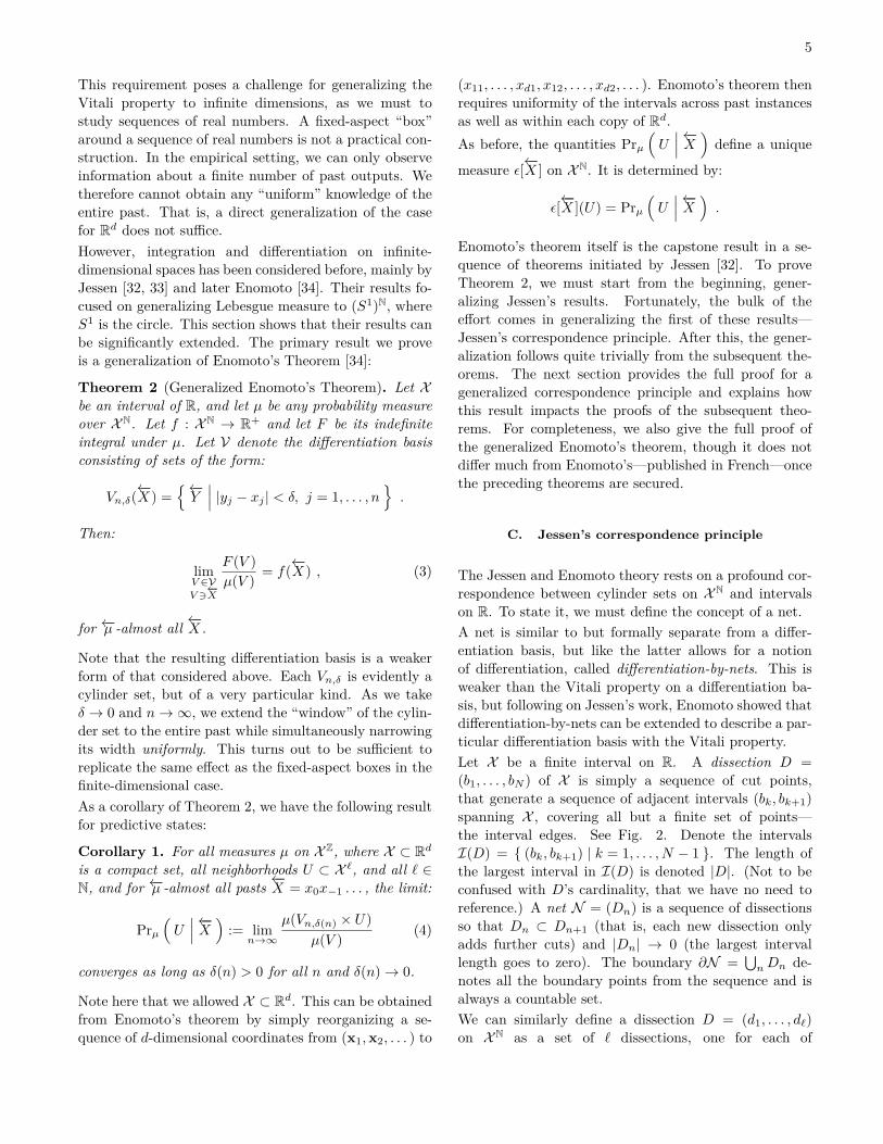
This requirement poses a challenge for generalizing theVitali property to infinite dimensions, as we must tostudy sequences of real numbers. A fixed-aspect “box”around a sequence of real numbers is not a practical con-struction. In the empirical setting, we can only observeinformation about a finite number of past outputs. Wetherefore cannot obtain any “uniform” knowledge of theentire past. That is, a direct generalization of the casefor Rd does not suffice.However, integration and differentiation on infinite-dimensional spaces has been considered before, mainly byJessen [32, 33] and later Enomoto [34]. Their results fo-cused on generalizing Lebesgue measure to (S1)N, whereS1 is the circle. This section shows that their results canbe significantly extended. The primary result we proveis a generalization of Enomoto’s Theorem [34]:

Theorem 2 (Generalized Enomoto’s Theorem). Let Xbe an interval of R, and let µ be any probability measureover XN. Let f : XN → R+ and let F be its indefiniteintegral under µ. Let V denote the differentiation basisconsisting of sets of the form:

Vn,δ(←−X ) =

←−Y∣∣∣ |yj − xj | < δ, j = 1, . . . , n

.

Then:

limV ∈VV 3←−X

F (V )µ(V ) = f(←−X ) , (3)

for ←−µ -almost all ←−X .

Note that the resulting differentiation basis is a weakerform of that considered above. Each Vn,δ is evidently acylinder set, but of a very particular kind. As we takeδ → 0 and n→∞, we extend the “window” of the cylin-der set to the entire past while simultaneously narrowingits width uniformly. This turns out to be sufficient toreplicate the same effect as the fixed-aspect boxes in thefinite-dimensional case.As a corollary of Theorem 2, we have the following resultfor predictive states:

Corollary 1. For all measures µ on X Z, where X ⊂ Rdis a compact set, all neighborhoods U ⊂ X `, and all ` ∈N, and for ←−µ -almost all pasts ←−X = x0x−1 . . . , the limit:

Prµ(U∣∣∣←−X )

:= limn→∞

µ(Vn,δ(n) × U)µ(V ) (4)

converges as long as δ(n) > 0 for all n and δ(n)→ 0.

Note here that we allowed X ⊂ Rd. This can be obtainedfrom Enomoto’s theorem by simply reorganizing a se-quence of d-dimensional coordinates from (x1,x2, . . . ) to

(x11, . . . , xd1, x12, . . . , xd2, . . . ). Enomoto’s theorem thenrequires uniformity of the intervals across past instancesas well as within each copy of Rd.As before, the quantities Prµ

(U∣∣∣←−X )

define a unique

measure ε[←−X ] on XN. It is determined by:

ε[←−X ](U) = Prµ(U∣∣∣←−X )

.

Enomoto’s theorem itself is the capstone result in a se-quence of theorems initiated by Jessen [32]. To proveTheorem 2, we must start from the beginning, gener-alizing Jessen’s results. Fortunately, the bulk of theeffort comes in generalizing the first of these results—Jessen’s correspondence principle. After this, the gener-alization follows quite trivially from the subsequent the-orems. The next section provides the full proof for ageneralized correspondence principle and explains howthis result impacts the proofs of the subsequent theo-rems. For completeness, we also give the full proof ofthe generalized Enomoto’s theorem, though it does notdiffer much from Enomoto’s—published in French—oncethe preceding theorems are secured.

C. Jessen’s correspondence principle

The Jessen and Enomoto theory rests on a profound cor-respondence between cylinder sets on XN and intervalson R. To state it, we must define the concept of a net.A net is similar to but formally separate from a differ-entiation basis, but like the latter allows for a notionof differentiation, called differentiation-by-nets. This isweaker than the Vitali property on a differentiation ba-sis, but following on Jessen’s work, Enomoto showed thatdifferentiation-by-nets can be extended to describe a par-ticular differentiation basis with the Vitali property.Let X be a finite interval on R. A dissection D =(b1, . . . , bN ) of X is simply a sequence of cut points,that generate a sequence of adjacent intervals (bk, bk+1)spanning X , covering all but a finite set of points—the interval edges. See Fig. 2. Denote the intervalsI(D) = (bk, bk+1) | k = 1, . . . , N − 1 . The length ofthe largest interval in I(D) is denoted |D|. (Not to beconfused with D’s cardinality, that we have no need toreference.) A net N = (Dn) is a sequence of dissectionsso that Dn ⊂ Dn+1 (that is, each new dissection onlyadds further cuts) and |Dn| → 0 (the largest intervallength goes to zero). The boundary ∂N =

⋃nDn de-

notes all the boundary points from the sequence and isalways a countable set.We can similarly define a dissection D = (d1, . . . , d`)on XN as a set of ` dissections, one for each of

6

D1

D2

D3⋮

I1(x)I2(x)

I3(x)

x

FIG. 2: Snapshot of a differentiation net. Adifferentiation net defined on a line segment.D1, D2, D3, . . . represents the dissections which

comprise the net. Each dissection contains the last; newpoints are indicated in red and old points in gray. Thesepoints define intervals; a sequence of these intervals is

shown, (Ik(x)), converging on the point x.

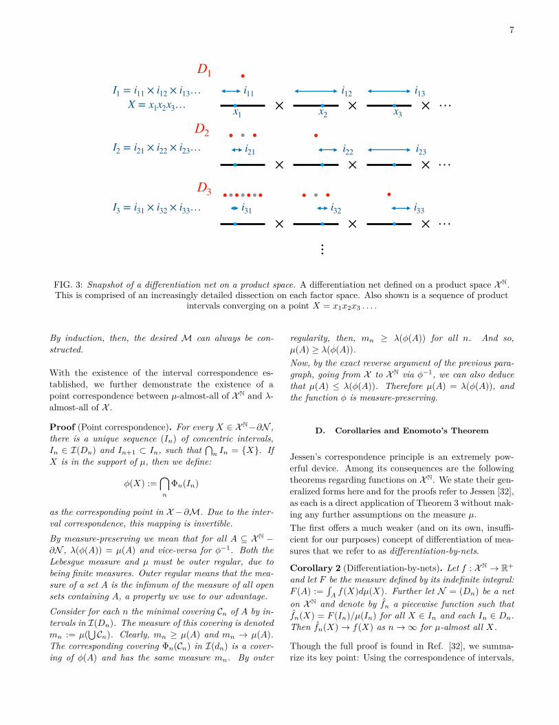
the first ` copies of X . D intervals I(D) =i1 × . . . i` ×XN

∣∣ ik ∈ I(dk)are the cylinder sets gen-

erated by the intervals of each individual dissection. SeeFig. 3. The boundary of a dissection is the set ofall points that do not belong to these intervals: ∂D =X ∈ XN

∣∣ ∃k : xk ∈ dk. The size of the dissection is

|D| := maxk |dk|. For a finite measure µ, there are alwaysdissections with µ(∂D) = 0 of any given |D| = maxk |dk|,since µ|X ` can only have at most countably many singu-lar points.A net N = (Dn = (d1,n, . . . , d`n,n)) of XN is a sequenceof dissections of increasing depth `n so that each se-quence (dk,n) for fixed k is a net for the kth copy ofX . ∂N =

⋃n ∂Dn denotes all the accumulated bound-

ary points of this sequence. Again, for finite measure µ,nets always exist that have µ(∂N ) = 0 for all n; netswith this property are called µ-continuous nets.Note that for any net, every sequence of intervals (In),In ∈ I(Dn) and In+1 ⊂ In, uniquely determines a pointX ∈ XN. If X 6∈ ∂D, then X uniquely determines asequence of intervals.The following result can be proven (generalized from Ref.[32]):

Theorem 3 (Generalized correspondence principle). LetX ⊂ R be an interval and let λ be the Lebesgue measureon X , normalized so λ(X ) = 1. Let µ be a finite measure

on XN that has no singular points. Let N = (Dn) beany µ-continuous net of XN. Then there exists a netM = (dn) of X so that:

1. There exists a function Φn that maps each intervalin I(Dn) of positive measure to one and only oneinterval in I(dn) and vice versa for Φ−1

n ;

2. λ(Φn(I)) = µ(I) for all I ∈ I(Dn) with µ(I) > 0;and

3. The mapping φ : XN−∂N → X−∂M, generated byX 7→ (In) 7→ (Φn(In)) 7→ x, is measure-preserving.

To summarize this technical statement: For any methodof indefinitely dissecting the set XN into smaller andsmaller intervals, there is in fact an “equivalent” suchmethod for dissecting the much simpler set X . It isequivalent in the sense that all the resulting intervals arein one-to-one correspondence with one another, a cor-respondence that preserves measure. Since interval se-quences uniquely determine points (and vice versa for aset of full measure), this induces a one-to-one correspon-dence between points that is also measure-preserving.The proof consists of two parts. The first proves thefirst two claims about M. Namely, there is an intervalcorrespondence and it is measure-preserving. The secondshows this extends to a correspondence between XN andX that is also measure-preserving.

Proof (Interval correspondence). The proof proceeds byinduction. For a given µ-continuous net N = (Dn), sup-pose we already constructed dissections d1, . . . , dN of Xso that a function Φn between positive-measure intervalsin Dn and dn exists with the desired properties (1) and(2) above, for all n = 1, . . . , N . Now, for Dn+1, a certainset of the intervals in I(Dn) is divided. Suppose I ∈ Individes into I ′ and I ′′. If either of these, say I ′′, has mea-sure zero then we discard it and set Φn+1(I ′) = Φn(I).Otherwise, suppose that Φn(I) = (a, b). Then divideΦn(I) into the intervals:

Φn+1(I ′) :=(a,aµ(I) + (b− a)µ(I ′)

µ(I)

)Φn+1(I ′′) :=

(aµ(I) + (b− a)µ(I ′)

µ(I) , b

),

that clearly have Lebesgue measures λ(Φn+1(I ′)) = µ(I ′)and λ(Φn+1(I ′′)) = µ(I ′′), respectively. Generalizing thisto more complicated divisions of I is straightforward.Now, we can always suppose for a given net N that D0is just the trivial dissection that makes no cuts and onlyone interval. However, this has a trivial correspondencewith X ; namely, Φ0(XN) = X .

7

×

×

×

×

×

×

×

×

× …

…

…x1 x2 x3

D1

D2

D3

X = x1x2x3…

⋮

I1 = i11 × i12 × i13… i11 i12 i13

i21 i22 i23

i31 i32 i33

I2 = i21 × i22 × i23…

I3 = i31 × i32 × i33…

FIG. 3: Snapshot of a differentiation net on a product space. A differentiation net defined on a product space XN.This is comprised of an increasingly detailed dissection on each factor space. Also shown is a sequence of product

intervals converging on a point X = x1x2x3 . . . .

By induction, then, the desired M can always be con-structed.

With the existence of the interval correspondence es-tablished, we further demonstrate the existence of apoint correspondence between µ-almost-all of XN and λ-almost-all of X .

Proof (Point correspondence). For every X ∈ XN−∂N ,there is a unique sequence (In) of concentric intervals,In ∈ I(Dn) and In+1 ⊂ In, such that

⋂n In = X. If

X is in the support of µ, then we define:

φ(X) :=⋂n

Φn(In)

as the corresponding point in X −∂M. Due to the inter-val correspondence, this mapping is invertible.By measure-preserving we mean that for all A ⊆ XN −∂N , λ(φ(A)) = µ(A) and vice-versa for φ−1. Both theLebesgue measure and µ must be outer regular, due tobeing finite measures. Outer regular means that the mea-sure of a set A is the infimum of the measure of all opensets containing A, a property we use to our advantage.Consider for each n the minimal covering Cn of A by in-tervals in I(Dn). The measure of this covering is denotedmn := µ(

⋃Cn). Clearly, mn ≥ µ(A) and mn → µ(A).

The corresponding covering Φn(Cn) in I(dn) is a cover-ing of φ(A) and has the same measure mn. By outer

regularity, then, mn ≥ λ(φ(A)) for all n. And so,µ(A) ≥ λ(φ(A)).Now, by the exact reverse argument of the previous para-graph, going from X to XN via φ−1, we can also deducethat µ(A) ≤ λ(φ(A)). Therefore µ(A) = λ(φ(A)), andthe function φ is measure-preserving.

D. Corollaries and Enomoto’s Theorem

Jessen’s correspondence principle is an extremely pow-erful device. Among its consequences are the followingtheorems regarding functions on XN. We state their gen-eralized forms here and for the proofs refer to Jessen [32],as each is a direct application of Theorem 3 without mak-ing any further assumptions on the measure µ.The first offers a much weaker (and on its own, insuffi-cient for our purposes) concept of differentiation of mea-sures that we refer to as differentiation-by-nets.

Corollary 2 (Differentiation-by-nets). Let f : XN → R+

and let F be the measure defined by its indefinite integral:F (A) :=

∫Af(X)dµ(X). Further let N = (Dn) be a net

on XN and denote by fn a piecewise function such thatfn(X) = F (In)/µ(In) for all X ∈ In and each In ∈ Dn.Then fn(X)→ f(X) as n→∞ for µ-almost all X.

Though the full proof is found in Ref. [32], we summa-rize its key point: Using the correspondence of intervals,

8

we write F (In)/µ(In) = F (Φ(In))/λ(Φ(In)), where F isthe indefinite integral of f φ−1 with respect to λ. Thelimit then holds due to the Vitali property of λ on X .However, we also note that Corollary 2 is not an exten-sion of the Vitali property to cylinder sets on XN. Jessenhimself offers a counterexample to this effect in a laterpublication [33].Jessen’s second corollary is key to demonstrating that V,the differentiation basis defined in Theorem 2, will havethe sought-after Vitali property.

Corollary 3 (Functions as limits of integrals). Let f :XN → R+, and let fn(X) be a sequence of functions givenby:

fn(x1x2 . . . ) :=∫Y ∈XN

f(x1 . . . xnY )dµ(Y ) .

That is, we integrated over all observations after the firstn. Thus, fn only depends on the first n observations.Then fn(X)→ f(X) as n→∞ for µ-almost all X.

This proof we also skip, again referring the reader toJessen [32], as no step is directly dependent on the mea-sure µ itself and only on properties already proven by theprevious theorems.We now have sufficient knowledge to prove the general-ized Enomoto’s theorem; generalized from Ref. [34].

Proof (Generalized Enomoto’s Theorem). First, wemust demonstrate, for almost every X, that there existsa sequence Vj(X) converging on X such that the limitholds. By Corollary 3, there must be, for µ-almost all Xand any ε > 0, a k(X, ε) such that |fn(X)− f(X)| < ε/2for all n > k(X, ε). Now, from the Vitali property on µnand the fact that fn only depends on the first n observa-tions, it must be true that for any ε > 0 and almost allX, there is a 0 < ∆(X,n, ε) < 1 so that:∣∣∣∣fn(X)− F (Vn,δ(X))

µ(Vn,δ(X))

∣∣∣∣ < ε/2 ,

whenever δ < ∆(X,n, ε). For a given ε, there is acountable number of conditions (one for each n). Assuch, the set of points X for which all conditions holdis still measure one. Then, taking for each X the in-teger K := k(X, ε) and subsequently the number ∆ :=∆(X, k(X, ε), ε), we can choose VK,∆(X) and by the tri-angle inequality we must have:∣∣∣∣f(X)− F (VK,∆(X))

µ(VK,∆(X))

∣∣∣∣ < ε . (5)

This completes the proof’s first part.However, the second part—that all sequences Vnj ,δj

(x) ofneighborhoods give converging likelihood ratios—further

follows from the above statements, as:∣∣∣∣f(X)−F (Vnj ,δj (X))µ(Vnj ,δj

(X))

∣∣∣∣ < ε

must hold for any nj > K(X, ε) and any δj <

∆(X,K(X, ε), ε), which must eventually be true for anyconverging sequence to X.

Now, the previous theorem does not directly prove theVitali property but rather bypasses it. Demonstratingthat the differentiation basis V may be used to recoverRadon-Nikodym derivatives. This, then, is sufficient forCorollary 1 to hold, guaranteeing the existence of predic-tive states ε[←−X ] for µ-almost all ←−X .

E. Remarks on convergence

An important task regarding predictive states is to learna process’s predictive states—that is, the ε-mapping fromobserved pasts to distributions over futures—from a suf-ficiently large sample of observations. These learned pre-dictive states may then be used to more accurately pre-dict the process’ future behavior based on behaviors al-ready observed.The previous three sections avoided constraining themeasure µ on XN to be anything other than finite. It wasnot assumed to be either stationary or ergodic, in par-ticular. In such cases the ε-mapping is time-dependent,as it obviously depends on where futures are split frompasts. To adequately reconstruct ε[←−X ] from a single, longobservation requires that the process be both stationaryand ergodic. Stationarity makes ε[←−X ] time-independent,and ergodicity ensures that the probabilities in the lim-its Eqs. (1) and (4) can be approximated by taking thetime-averaged frequencies of occurrence.The next natural question is how rapidly convergenceoccurs for each past, in a given process. So far, we onlyguaranteed that convergence exists, but said nothing onits rate. This is process-dependent. Section V givesseveral examples of processes and process types withtheir convergence rate. The most useful way to think ofthe rate is in the form of “probably-almost-correct”-typestatements, as exemplified in the following result:

Proposition 2. Let µ be a probability measure on X `.Let ηn,δ[

←−X ](U) = µ(Vn,δ×U)/µ(Vn,δ). For every cylinder

set U and ∆1,∆2 > 0, we have for sufficiently large ` andsmall δ:

Pr←−µ( ∣∣∣η`,δ[←−X ](U)− ε[←−X ](U)

∣∣∣ > ∆1

)< ∆2 .

9

That is, the probability of an error beyond ∆1 is less than∆2.

This is a consequence of the fact that all ←−X must even-tually converge. The possible relationships between ∆1,∆2, and ` in particular is explored in our examples.

IV. PREDICTIVE STATES FORM A HILBERTSPACE

Thus far, we demonstrated that for discrete and real X ,measures over XN possess a well-defined feature calledpredictive states that relate how past observations con-strain future possibilities. These states are defined byconvergent limits that can be approximated from empiri-cal time series in the case of stationary, ergodic processes.We turn our attention now to the topological and geomet-ric structure of these states, the spaces they live in, andhow the structure of these spaces may be leveraged in theinference process. The results make contact between pre-dictive states as elements of a Hilbert space and the well-developed arena of reproducing kernel Hilbert spaces. Todo this we introduce several new concepts.Denote the set of real-valued continuous functions on X Z

by C(X Z). The set of signed measures on X Z, that wecall M(X Z), may be thought of as dual to C(X Z). Thisallows us to define a notion of convergence of measureson X Z in relation to continuous functions. We say thata sequence of measures µn converges in distribution if:

limn→∞

∫F (X)dµn(X) =

∫F (X)dµ(X)

for all F ∈ C(X Z). Convergence in distribution is some-times referred to as weak convergence but we avoid thisvocabulary to minimize confusion—as another, distinctkind of weak convergence is needed in the Hilbert spacesetting.A kernel k : X Z×X Z → R generates a reproducing kernelHilbert space (RKHS) H if k(·, ·) is positive semi-definiteand symmetric [35]. H is typically defined as a spaceof functions (from X Z → R), but the kernel allows em-bedding measures on X Z into the function space throughfµ(x) =

∫k(x, y)dµ(y). This elicits an inner product

between any two positive measures µ and ν:

〈fµ|fν〉k :=∫ ∫

k(x, y)dµ(x)dν(y) .

The inner-product space on measures generated by thisconstruction is isometric to the RKHS generated byk(·, ·). The embedding of measures into this space isunique if the kernel is characteristic. And, convergence

in the norm of the Hilbert space is equivalent to con-vergence in distribution whenever the kernel is universal[36].What exactly is the set H of functions? The equivalenceof convergence in norm and convergence in distributiontempts identifying H with the space of continuous func-tions, but this is overly optimistic. If it were true—thatH = C(X Z)—then the convergence 〈F |fµn

〉 → 〈F |fµ〉for every F ∈ H implies µn → µ in norm. This, though,identifies norm convergence on the Hilbert space withweak convergence, which for Hilbert spaces is identifiedas the convergence of every inner product.For infinite-dimensional Hilbert spaces, these two typesof convergence cannot be identified. This is illustratedby the simple case of any orthogonal basis ei, for which〈F |ei〉 → 0 is necessary for F to have a finite norm, eventhough ‖ei‖ → 1 by definition. So, while convergence inthe norm ofH is equivalent to convergence in distributionof measures, we must conclude that H can only be aproper subspace of the continuous functions; a fact alsonoted in [37].

A. Topology of predictive states

Let the (closure of the) set of a process’s predictive statesbe denoted by:

K(µ) :=ε[←−X ]

∣∣∣←−X ∈ XN.

The closure is taken under convergence in distribution.The relation between pasts and predictive states may behighly redundant. For instance, in the process generatedby the results of a random coin-toss, since the futureobservations do not depend on past observations, K(µ)is trivial. Meanwhile, for a periodic process of periodk, K(µ) has k elements, corresponding to the k distinctstates—the process’ phases. In more complex cases, K(µ)may have countable and uncountable cardinality.We may also consider the vector space of signed measuresgenerated by the closed span ofK(µ), denotedK(µ). Thisis the smallest closed vector space that contains the pre-dictive states. This, too, may demonstrate redundancyin the form of linear dependence, regardless of the car-dinality of K(µ). For instance, it is possible to have anuncountably infinite set of predictive states K(µ) whosedimension, dimK(µ), is finite. In fact, it is the generalcase that any process generated by an HMM or GHMMwill have finite dimensional K(µ), but is not guaranteedto have finite K(µ) [12]. See Fig. 4.The topology of convergence in distribution is closely re-lated to the definition of continuity on XN. It behooves

10

𝕂(μ)

FIG. 4: Predictive states and their closed span. The reddots are a hypothetical set K(µ) of predictive states(shaped like the Sierpinski set) that is uncountablyinfinite but that has a finite-dimensional closed span

K(µ).

us at this juncture to discuss XN not only as a topologicalspace but also as a metric space.

Two useful families of distance metrics, equivalent to theproduct topology on XN, are the Euclidean metrics, onefor the discrete and real case each:

DE,γ(X,Y )2 :=∑∞

t=1(1− δxtyt)γ2t X discrete∑∞

t=1 ‖xt − yt‖2γ2t X ⊂ Rd

,

for some 0 < γ < 1. These distance metrics arise fromembedding XN in a Hilbert space. Given an orthogo-nal basis (ei), the components of this embedding for thediscrete case are given by:

ci(X) =γbi/|X |c xbi/|X |c = i mod |X |0 otherwise

and in the continuous case (X ⊂ Rd) by:

ci(X) = γtxk,t, i = k mod d .

Using these distance metrics, the following section intro-duces an inner product structure on K(µ) whose normmetrizes the topology of convergence in distribution.Once K(µ)’s natural embedding into a Hilbert space ofits own is established, we investigate how well this em-bedding can be approximated by the approach of repro-ducing kernel Hilbert spaces.

B. Embedding predictions in a Hilbert space

The space K(µ) of predictive states is a subspace P(XN)of the probability measures over XN. On P(XN), givenany symmetric positive-definite kernel k : XN×XN → R,we can define an inner product over measures:

〈µ, ν〉k :=∫ ∫

k(X,Y )dµ(X)dν(Y ) . (6)

Positive-definite means that for any finite set Xi ofXi ∈ XN and any set ci of values ci ∈ R, both setshave the same cardinality:∑

i,j

k(Xi, Xj)cicj ≥ 0 ,

with equality only when ci = 0 for all i. If this is true,then the inner product Eq. (6) is positive-definite for allmeasures. That is, 〈µ, µ〉k ≥ 0 with equality only whenµ = 0 [36].Since XN is compact, if the kernel k satisfies the prop-erty of being universal, then norm convergence under theinner product defined by k is equivalent to convergencein distribution of measures [36]. A simple example ofa universal kernel is the Gaussian radial basis function,when paired with an appropriate distance—namely, onedefined from embedding XN in a Hilbert space, as ourDE,γ are [38]. These take the form:

kβ,γ(X,Y ) := exp(−DE,γ(X,Y )2

β2

).

We denote the associated inner products by 〈·, ·〉β,γ .Hβ,γ :=

(P(XN), 〈·, ·〉β,γ

)defines a Hilbert space, since

it has the topology of convergence in distribution andP(XN) is complete in this topology.When referring to a measure µ as an element of Hβ,γwe denote it |µ〉β,γ and inner products in the bra-ket are〈µ|ν〉β,γ . Now, it should be noted that to every ket |µ〉β,γthere is a bra 〈µ|β,γ that denotes a dual element. How-ever, the dual elements of P(XN) correspond to contin-uous functions. The function fµ corresponding to 〈µ|β,γis given by:

fµ(X) :=∫kβ,γ(X,Y )dµ(Y ) , (7)

so that:

〈µ|ν〉β,γ =∫fµ(X)dν(Y ) .

Let Fβ,γ denote the space of all fµ that can be con-structed from Eq. (7). This function space, when paired

11

with the inner product 〈fµ, fν〉 := 〈ν|µ〉, is isomorphicto Hβ,γ . Fβ,γ is then a reproducing kernel Hilbert spacewith kernel kβ,γ .

As the start of Section IV discussed, Fβ,γ ⊂ C(XN). Fur-thermore, the Fβ,γ are not identical to one another, obey-ing the relationship Fβ,γ ⊂ Fβ′,γ when β > β′ [39]. How-ever, it is also the case that each Fβ,γ is dense in C(XN),so their representative capacity is still quite strong [36].

We note an important rule regarding the scaling of our in-ner products, as constructed. The distances DE,γ(X,Y )have finite diameter on our spaces. Let ∆ denote thediameter of X . For discrete X we simply have ∆ = 1;for X ⊂ Rd, ∆ is determined by the Euclidean distance.Then XN’s diameter is given by ∆/

√1− γ2. Since the

Gaussian is bounded below by 1−D2γ/β

2, for arbitrarilylarge β:

‖µ− ν‖2β,γ ≤‖µ− ν‖TV∆2

(1− γ2)β2 +O(β−3) , (8)

where ‖·‖β,γ is simply the norm of Hβ,γ and ‖·‖TV is thetotal variation norm. This tells us that the norm is lessdiscriminating between measures as β → ∞. Naturally,this can be remedied by rescaling the kernel with a β2

factor. As it happens, Eq. (8) will be useful later.

C. Finite-length embeddings

Our goal is to study how reproducing kernel Hilbertspaces may be used to encode information about predic-tive states gleaned from empirical observations. Giventhat such observations are always finite in length, wemust determine whether and in what manner the Hilbertspace representations of measures over finite-length ob-servations converges to the Hilbert space representationof a measure over infinite sequences.

Let µ` denote the measure µ restricted to X `. Define therestricted distance on X `:

D(`)E,γ(X,Y )2 :=

∑`t=1(1− δxtyt

)γ2t X discrete∑`t=1 ‖xt − yt‖

2γ2t X ⊂ Rd

,

for X,Y ∈ X `. This gives an important Pythagoreantheorem for sequences:

DE,γ(X,Y )2 =D(`)E,γ(x1 . . . x`, y1 . . . y`)2

+ γ2`DE,γ(x`+1 . . . , y`+1 . . . )2. (9)

Now, using D(`)E,γ define kernels k(`)

β,γ in the same style asfor XN. These generate inner products on P(X `). Denote

byH(`)β,γ the resulting Hilbert spaces. These are related to

the original Hβ,γ by the following factorization theorem:

Proposition 3. The predictive Hilbert space Hβ,γ fac-tors into H(`)

β,γ ⊗Hβγ−`,γ .

Before stating the proof, we should explain the above.The factorization Hβ,γ = H(`)

β,γ⊗Hβγ−`,γ denotes a sepa-ration of the infinite-dimensional Hβ,γ into two pieces—one of which is finite-dimensional, but retains the samekernel parameters and another reparametrize infinite-dimensional Hilbert space. The reparametrization is β →βγ−`. This constitutes, essentially, a renormalization-group technique, in which the the topology of wordsstarting at depth ` is equivalent to a reparametriza-tion of the usual topology. This reparametrization worksprecisely due to the Pythagorean theorem for sequencesEq. (9).

Proof. We are demonstrating an isomorphism—a par-ticularly natural one. Let δX be the Dirac delta measureconcentrated on X. We note that for any measure µ:

|µ〉β,γ =∫|δX〉β,γ dµ(X) .

Now, consider the linear function from Hβ,γ to H(`)β,γ ⊗

Hβγ−`,γ that maps:

|δX〉β,γ 7→ |δx1...x`〉(`)β,γ ⊗ |δx`+1...〉βγ−`,γ

,

for every X. Then by Eq. (9) we can see that this pre-serves the inner product and so is an isomorphism.

Note that for any of these Hilbert spaces there exists anelement corresponding to the constant function 1(X) =1 for all X. This function always exists in Fβ,γ . Wedenote its corresponding element in Hβ,γ as 〈1|β,γ , sothat 〈1|µ〉β,γ = 1 for all µ. Then the operator Π(`)

β,γ :Hβ,γ → H(`)

β,γ is given by:

Π(`)β,γ := I(`) ⊗ 〈1|β,γ ,

where I(`) is the identity on H(`)β,γ . It provides the canon-

ical mapping from a measure µ to its restriction µ`: Thatis, Π(`)

β,γ |µ〉β,γ = |µ`〉(`)β,γ .Consider the “truncation error”—that is, the residual er-ror remaining when representing a measure by its trun-cated form µ` rather than by its full form µ. We quantifythis in terms of an embedding. That is, there exists anembedding of truncated measures P(X `) into the spaceof full measures P(XN) such that the distance betweenany full measure and its truncated embedding is small:

12

Theorem 4. There exist isometric embeddings H(`)β,γ 7→

H(`′)β,γ and H(`)

β,γ 7→ Hβ,γ for any ` ≤ `′. Furthermore,let µ be any measure and µ` be its restriction to the first` observations, and let |µ`〉β,γ be the embedding of µ`into Hβ,γ . Then |µ`〉β,γ → |µ〉β,γ as ` → ∞, with ‖µ −µ`‖β,γ ∼ O(β−1γ`).

Proof. Let λβ,γ ∈ P(XN) denote the measure such that〈λβ,γ |β,γ = 〈1|β,γ for a given β, γ. For a measure µ withrestriction µ` let µ` denote the measure on XN with theproperty:

µ`(A×B) = µ`(A)λβγ−`,γ(B) ,

for A ∈ X ` and B ∈ XN. Then the mapping µ` 7→ µ` isan isomorphism, since:

〈µ`|ν`〉β,γ =∫ ∫

kβ,γ(X,Y )dµ`(X)dν`(X)

=∫ ∫

k(`)β,γ(x1 . . . x`, y1 . . . y`)dµ`dν`

×∫ ∫

kβγ−`,γ(x` . . . , y` . . . )dλβγ−`,γdλβγ−`,γ

= 〈µ`|ν`〉(`)β,γ∫dλβγ−`,γ

= 〈µ`|ν`〉(`)β,γ .

Now, as a result of Eq. (9), note that for any two mea-sures µ and ν:

〈µ, ν〉 =∫dµ`(x1 . . . x`)

∫dν`(y1 . . . y`) exp

(−β2D(`)

γ (x1 . . . x`, y1 . . . y`))〈µ(·|x1 . . . x`), ν(·|y1 . . . y`)〉βγ`,γ

If we combine this fact with the bound Eq. (8), we have the result:

‖µ− µ`‖2β,γ =∫dµ`(x1 . . . x`)

∫dµ`(y1 . . . y`) exp

(−β2D(`)

γ (x1 . . . x`, y1 . . . y`))‖µ(·|x1 . . . x`)− µ`(·|y1 . . . y`)‖2βγ−`

≤∫dµ`(x1 . . . x`)

∫dµ`(y1 . . . y`)

‖µ− µ`‖TV∆2γ2`

(1− γ2)β2 = ‖µ− µ`‖TV∆2γ2`

(1− γ2)β2 .

Thus, ‖µ− µ`‖β,γ ∼ O(β−1γ`).

In summary, representing measures µ over XN by theirtruncated forms µ` leads to a Hilbert space represen-tation that admits an approximate isomorphism to thespace of full measures. The resulting truncation error isof order O(β−1γ`).We close this part with a minor note about a lower boundon the distance between measures. Given a word w, thefunction on X ` that equals 1 when X = w and zerootherwise has a representation |w〉(`)β,γ in H(`)

β,γ . (Thisfollows since for finite X , all functions on X ` belongto F (`)

β,γ .) The extension of this to Hβ,γ is |w〉β,γ :=|w〉(`)β,γ ⊗ |λβ,γ〉βγ−`,γ . This has the convenient propertythat 〈w|µ〉β,γ = Prµ ( w ). Then, by the Cauchy-Schwarzinequality, for any measures µ and ν and any word w:

‖µ− ν‖β,γ ≥| 〈w|µ− ν〉 |√〈w|w〉β,γ

= |Prµ ( w )− Prν ( w )|√〈w|w〉β,γ

. (10)

So, word probabilities function as lower bounds on the

Hilbert space norm.

D. Predictive states from kernel Bayes’ rule

A prominent use of reproducing kernel Hilbert spaces isto approximate empirical measures [40]. Given a measureµ over a space X and N samples Xk drawn from thisspace, one constructs an approximate representation ofµ via:

|µ〉 := 1N

N∑k=1|δXk〉 .

In other words, µ is approximated as a sum of delta func-tions centered on the observations. Convergence of thisapproximation to |µ〉 is (almost surely) O(N−1/2) [40].This fact, combined with our Theorem 4, immediatelygives the following result for Hβ,γ :

Proposition 4. Suppose for some µ ∈ P(XN) we takeN samples of length `, denoted Xk ∈ X ` (k = 1 . . . N),

13

and construct the state:

|µ`,N 〉β,γ = 1N

N∑k=1|δXk〉(`)β,` ⊗ |λβγ−`,γ〉βγ−`,γ

.

Then |µ`,N 〉β,γ → |µ〉 converges almost surely as N, ` →∞ with error O(N−1/2 + β−1γ`).

A more nuanced application of RKHS for measures lies inreconstructing conditional distributions [26–28, 40, 41].Let µ be a joint measure on some X ×Y, and let µ|X andµ|Y be its marginalizations. Given N samples (Xk, Yk),construct the covariance operators:

CXX := 1N

∑k

|δXk〉 〈δXk

| and

CY X := 1N

∑k

|δYk〉 〈δXk

| .

Let µY|X be the conditional measure for X ∈ X .For some g ∈ HY—the RKHS constructed on Y—letFg(X) := 〈g|µY|X〉 be a function on X . If Fg ∈ HXfor all g ∈ HY , then CY X

(CXX − ζI

)−1|δX〉 converges

to |µY|X〉 as N → ∞, ζ → 0, with convergence rateO((Nζ)−1/2 + ζ1/2).

The requirement essentially tells us that the structure ofthe conditional measure is compatible with the structuresrepresented by the RKHS.This is the kernel Bayes’ Rule [41]. It applies to ourHβ,γ , by combining it with our results on truncated rep-resentations:

Theorem 5. Let µ ∈ P(X Z) be a stationary and ergodicprocess. Suppose we take a long sample X ∈ XL and fromthis sample subwords of length 2`, wt = xt−`+1 . . . wt+`for t = `, . . . , L − `. (There are L− 2` + 1 such words.)Split each word into a past ←−w t = xt−`+1 . . . wt and afuture −→w t = xt+1 . . . xt+`, each of length `. Define theoperators:

C(←−X←−X)β,γ = 1

L− 2`+ 1

L−∑t=`|δ←−w t〉β,γ⊗ |δ←−w t

〉β,γ

and

C(←−X−→X)β,γ = 1

L− 2`+ 1

L−∑t=`|δ←−w t〉β,γ⊗ |δ−→w t

〉β,γ

.

Now, suppose for every g ∈ Fβ,γ that⟨ε[←−X ], g

⟩∈ Fβ,γ

and⟨η`[←−X ], g

⟩→⟨ε[←−X ], g

⟩at a rate of O(h←−

X(`)); see

Section III E. Then for all ←−X :

C(←−X−→X)β,γ

(C

(←−X←−X)β,γ − ζ · Iβ,γ

)−1|δ←−X〉β,γ

almost surely converges to |ε[←−X ]〉β,γ as L →∞, ` → ∞, and ζ → 0, at the rateO((Lζ)−1/2 + ζ1/2 + γ−` + h←−

X(`)).

This integrates all our results thus far with the usual ker-nel Bayes’ rule. Several observations are in order. First,there will (←−µ -almost) always be an h←−

X(`) as required

by this theorem due to our own Thm. 1 and Cor. 1.Second, since ε[←−X ] is not generally continuous, the theo-rem’s strict requirements on ε[←−X ] are not satisfied. Thatsaid, weaker versions hold. If

⟨ε[←−X ], g

⟩as a function

of ←−X does not belong to Fβ,γ as a function of ←−X , thenthe representational error scaling depends on the preciseform of ε[←−X ]. The latter can be obtained by choosing theζ-parameter through cross-validation analysis [40, 41].

V. EXAMPLES

We close with a handful of examples and case studiesthat give further insight to the convergence of

∥∥η`[←−X ]−ε[←−X ]

∥∥β,γ

for widely-employed process classes—Markov,hidden Markov, and renewal processes.

A. Order-R Markov processes

A Markov process is a stochastic process where each ob-servation xt statistically depends only on the previous ob-servation xt−1. An order-R Markov process is one whereeach observation xt depends only on the previous R ob-servations xt−R . . . xt−1. As such, the predictive statesare simply given by:

Prµ(x∣∣∣←−X )

= Prµ ( x−R+1 . . . x0x )Prµ ( x−R+1 . . . x0 ) ,

for each ←−X = x0x−1 . . . . Since the predictive state isentirely defined after a finite number of observations, andthis number is bounded by R, there is no conditioningerror when R is taken as the observation length.

B. Hidden Markov processes

A hidden Markov model (HMM) (S,X ,

T(x) ) is de-fined here as a finite set S of states, a set X of obser-vations, and a set T(x) = (T (x)

ss′ ) of transition matrices,labeled by elements x ∈ X and whose components areindexed by S [21]. The elements are constrained so that0 ≤ T

(x)ss′ ≤ 1 and

∑x,s′ T

(x)ss′ = 1 for all s, s′ ∈ S. Let

T =∑x T(x) and π be its left-eigenvector such that

14

πT = π. HMMs generate a stochastic process µ definedby the word probabilities:

Prµ ( x1 . . . x` ) :=∑s′

[πT(x1) . . .T(x`)

]s′.

An extension of HMMs, called generalized hidden Markovmodels (GHMMs) [21] (or elsewhere observable operatormodels [22]), is defined as (V,X ,

T(x) ) where V is

a finite-dimensional vector space. The only constrainton the transition matrices T(x) is that T have a simpleeigenvector of eigenvalue 1, the left-eigenvector is stilldenoted π, the right-eigenvector denoted φ, and the wordprobabilities:

Prµ ( x1 . . . x` ) := πT(x1) . . .T(x`)φ

are positive [21]. GHMMs generate a strictly broaderclass of processes than finite hidden Markov models can[21, 22, 42], though their basic structure is very similar.First off, consider sofic processes. A sofic process is onethat is not Markov at any finite order, but that is stillexpressible in a certain finite way. Namely, a sofic pro-cess is any that can be generated by a finite-state hiddenMarkov model with the unifilar property. An HMM hasthe unifilar property if T (x)

s′s > 0 only when s′ = f(x, s)for some deterministic function f : S × X → S. UnifilarHMMs are the stochastic generalization of deterministicfinite automata in computation theory [43].The most useful property of sofic processes is that thestates of their minimal unifilar HMM correspond exactlyto the predictive states, of which there is always a finitenumber. Unlike with order-R Markov processes, there isno upper bound to how many observations it may taketo δ-synchronize the predictive states. However, closed-form results on the synchronization to predictive statesfor unifilar HMMs is already known: at L past observa-tions, with L → ∞, the conditioning error is exponen-tially likely (in L) to be exponentially small (in L) [24].In terms of our Hilbert space norm, there are constantsα and C such that

Pr←−µ( ∥∥∥ηx1...x`

− ε[←−X ]∥∥∥β,γ

> α`)< Cα` .

As such, for ←−µ -almost-all pasts, the corresponding con-vergence rate for the kernel Bayes’ rule applied to a soficprocess is O

((Lζ)−1/2 + ζ1/2 + min(α, γ)−`

).

Not all discrete-observation stochastic processes can begenerated with a finite-state unifilar hidden Markovmodel. Though still encompassing only a small slice ofprocesses, generalized hidden Markov models have a con-siderably larger scope of representation than finite unifi-lar models, as noted above.

The primary challenge in this setting is to relate thestructure of a given HMM to the predictive states of itsprocess. This is achieved through the notion of mixedstates. A mixed state ρ is a distribution over the statesof a finite HMM. A given HMM, with the stochastic dy-namics between its own states, induces a higher-orderdynamic on its mixed states and, critically for analysis,this is an iterated function system (IFS). Under suitableconditions the IFS has a unique invariant measure, andthe support of this measure maps surjectively onto theprocess’ set of predictive states. See Refs. [12] for detailson this construction.If ρ = (ρ) is a mixed state, then the updated mixed stateafter observing symbol x is:

f (x)s (ρ) := 1∑

s′

[T(x)ρ

]s′

[T(x)ρ

]s.

Let the matrix[Df (x)]

s′s(ρ) be given by the Jacobian

∂f(x)s′ /∂ρs at a given value of ρ. There is a statistic, called

the Lyapunov characteristic exponent λ < 0, such that:

λ = lim`→∞

1`

log∥∥Df (x`)(ρ`) · · ·Df (x1)(ρ1)v

∥∥‖v‖ ,

where ρt := f (xt−1)· · ·f (x1)(ρ), for any vector v tangentto the simplex, almost any ρ (in the invariant measure),and almost any −→X = x1x2 . . . (in the measure of the pre-diction induced by ρ). The exponent λ then determinesthe rate at which conditioning error for predictive statesconverges to zero: for all ε and sufficiently large `:

Pr←−µ( ∥∥∥ηx1...x`

− ε[←−X ]∥∥∥β,γ

< Ceλ`)> 1− ε .

This is somewhat less strict—depending on how rapidlythe Lyapunov exponent converges in probability. Inany case, for ←−µ -almost all pasts, the convergence of thekernel Bayes’ rule is O

((Lδ)−1/2 + δ1/2 + min(λ, γ)−`

),

very similar to the sofic process rate.We anticipate that these rules still broadly apply to gen-eralized hidden Markov models, though we recommendmore detailed analysis on this question.

C. Renewal processes

A renewal process, usually defined over continuous-time,can be defined for discrete time as follows. A renewalprocess emits 0s for a randomly selected duration beforeemitting a single 1 and then randomly selecting a newduration to fill with 0s [44]. Renewal processes can be assimple as Poisson processes, where the probability at any

15

moment of producing another 0 or restarting on 1 is in-dependent of time. Or, they can be far more memoryful,with a unique predictive state for any number of past 0s.

While high-memory renewal processes cannot generallybe represented by a finite hidden Markov model, theyhave only a countable number of predictive states, unlikemost hidden Markov models. This follows since everynumber of past 0s defines a potential predictive state,but the process has no further memory beyond the mostrecent 1. Said simply, the predictive states are the timesince last 1—or some coarse-graining of this indicator inspecial cases, such as the Poisson process.

A renewal process is specified by the survival probabilityΦ(n) that a contiguous block of 0s has length at leastn. The exact probability of a given length is F (n) :=Φ(n) − Φ(n + 1). It is always assumed that Φ(1) = 1.Further, stationarity requires that m :=

∑∞n=1 Φ(n) be

finite, as this gives the mean length of a block of 0s. Inthe most general case the predictive states are given by:

ε[←−X ] =εk

←−X = 0k1 . . .

undefined ←−X = 0∞

,

where the measures εk are recursively defined by the wordprobabilities:

Prεk

(0`1w

)= F (k + `)

Φ(k) Prε0 ( w ) .

Now, it can be easily seen that each past ←−X convergesto zero conditioning error at a finite length since (al-most) all pasts have the structure . . . 10k, and so onlythe most recent k + 1 values need be observed to knowthe predictive state. Therefore the kernel Bayes’ rulehas an asymptotic convergence rate for each past ←−X ofO((Lδ)−1/2 + δ1/2 + γ−`

). However, this does not tell

the entire story, as obviously not all pasts converge uni-formly. A probabilistic expression of the conditioningerror gives more information:

Proposition 5. Suppose µ is a renewal process withΦ(n) ∝ n−α, α > 1. Then there exist constants C andK such that:

Pr←−µ( ∥∥∥ηx1...x`

− ε[←−X ]∥∥∥β,γ

> C`−1)> K`−α .

That is, the probability the conditioning error decays as1/` is itself at least power-law decaying in `.

Proof. Recall from Eq. (10):∥∥∥ηx1...x`− ε[←−X ]

∥∥∥β,γ

>

∣∣∣Prµ ( w | x1 . . . x` )− Prµ(w∣∣∣←−X )∣∣∣√

〈w|w〉β,γ,

for every word w, so we can choose any w and obtain alower bound on the conditioning error. If our past ←−X hasthe form 0k1 . . . for k < `, then we are already synchro-nized to the predictive state and the conditioning erroris zero. Thus, we are specifically interested in the casek ≥ ` and we will further consider the large-` limit.Now, under our assumptions, Φ(n) = n−α for some con-stant Z. For large n, F (n) ∼ αn−α−1. Then for anyj:

Prµ(

0j1∣∣∣←−X )

= F (k + j)Φ(k) ∼ α

k

(k + j

k

)−α−1.

Meanwhile, so long as k ≥ `, the truncated prediction hasthe form:

Prµ(

0j1∣∣ 0`

)=∞∑n=1

Φ(n+ `)∑p Φ(p+ `)

F (n+ `+ j)Φ(n+ `)

= Φ(`+ j)∑p Φ(p+ `) ∼

α− 1`

(`+ j

`

)−α.

Now, choose 0 < C < α− 1 and define:

B =(

1− C + 1α

)−1.

Then it can be checked straightforwardly that wheneverk > B`, we have:

Prµ(

1∣∣ 0`

)− Prµ

(1∣∣∣←−X )

∼ 1`

[α

(1− `

k

)− 1]

>C

`.

The probability that k > B` is given by Φ(B`) =B−α`−α. Setting K = B−α/

√〈1|1〉β,γ proves the the-

orem.

Therefore, while every sequence←−X converges to zero con-ditioning error at finite length, this convergence is notuniform, to such a degree that the proportion of paststhat retain conditioning error of 1/` has a fat tail in`. This is a matter of practical importance that is notcleanly expressed in the big-O expression of the condi-tioning error from Thm. 5.

16

Poisson and renewal processes are only the first and sec-ond rungs of the hierarchy of hidden semi-Markov pro-cesses [44]. Loosely speaking these are state-dependentrenewal processes. The preceding Hilbert space frame-work extends to this larger process class—a subject re-counted elsewhere.

VI. CONCLUDING REMARKS

Taken altogether, the results fill-in important gaps inthe foundations of predictive states, while strengthen-ing those foundations for further development, extension,and application. Previously, predictive states were onlyexamined in the context of hidden Markov models, theirgeneralizations, and hidden semi-Markov models. Weprovided a definition applicable to any stationary andergodic process with discrete and real-valued observa-tions. Furthermore, we showed that predictive statesfor these processes are learnable from empirical data,whether through a direct method of partitioning pasts orthrough indirect methods, such as the reproducing kernelHilbert space.

One important extension is to continuous-time pro-cesses. By exploiting the full generality of Jessen’s andEnomoto’s theorems we believe this extension is quitefeasible. As long as the set of possible pasts and futuresconstitutes a separable space, they should be expressiblein the form of a countable basis, to which these theoremsmay then be applied. The challenge lies in constructingan appropriate and useful basis. We leave this for futurework.

We described key properties of the space in which pre-

dictive states live. However, predictive states are notmerely static objects. They predict the probabilities offuture observations. And, once those observations aremade, the predictive state may be updated to accountfor new information. Thus, predictive states provide thestochastic rules for their own transformation into futurepredictive states. This dynamical process has been ex-plored in great detail in the cases where the process isgenerated by a finite hidden Markov model—this is foundin former work on the ε-machine and the mixed statesof HMMs. Understanding the nature of this dynamicfor more general processes, including how it makes con-tact with other dynamical approaches—such as, stochas-tic differential equations in the continuous-time setting—also remains for future work.

ACKNOWLEDGMENTS

We thank Nicolas Brodu and Adam Rupe for helpful com-ments and revisions. We also thank Alex Jurgens, GregWimsatt, Fabio Anza, David Gier, Kyle Ray, MikhaelSemaan, and Ariadna Venegas-Li for helpful discussions.JPC acknowledges the kind hospitality of the TellurideScience Research Center, Santa Fe Institute, Institute forAdvanced Study at the University of Amsterdam, andCalifornia Institute of Technology for their hospitalityduring visits. This material is based upon work sup-ported by, or in part by, Grant Nos. FQXi-RFP-IPW-1902 and FQXi-RFP-1809 from the Foundational Ques-tions Institute and Fetzer Franklin Fund (a donor-advisedfund of Silicon Valley Community Foundation), grantTWCF0570 from the Templeton World Charity Founda-tion, grants W911NF-18-1-0028 and W911NF-21-1-0048from the U.S. Army Research Laboratory and the U.S.Army Research Office, and grant DE-SC0017324 fromthe U.S. Department of Energy.

[1] J. P. Crutchfield. Between order and chaos. NaturePhysics, 8(January):17–24, 2012. 1

[2] A. B. Boyd and J. P. Crutchfield. Maxwell demon dy-namics: Deterministic chaos, the Szilard map, and theintelligence of thermodynamic systems. Phys. Rev. Let.,116:190601, 2016. 1

[3] S. Loomis and J. P. Crutchfield. Thermal efficiencyof quantum memory compression. Phys. Rev. Lett.,125:020601, 2020.

[4] A. Jurgens and J. P. Crutchfield. Functional thermo-dynamics of maxwellian ratchets: Constructing and de-constructing patterns, randomizing and derandomizingbehaviors. Phys. Rev. Res., 2(3):033334, 2020. 1

[5] M. Gu, K. Wiesner, E. Rieper, and V. Vedral. Quantummechanics can reduce the complexity of classical models.Nature Comm., 3(762):1–5, 2012. 1

[6] J. R. Mahoney, C. Aghamohammadi, and J. P. Crutch-field. Occam’s quantum strop: Synchronizing and com-pressing classical cryptic processes via a quantum chan-nel. Scientific Reports, 6:20495, 2016.

[7] F. C. Binder, J. Thompson, and M. Gu. A practical,unitary simulator for non-Markovian complex processes.arXiv.org:1709.02375.

[8] A. Venegas-Li, A. Jurgens, and J. P. Crutchfield.Measurement-induced randomness and structure in con-trolled qubit processes. Phys. Rev. E, 102(4):040102(R),2020. 1

[9] J. P. Crutchfield and D. P. Feldman. Statistical complex-ity of simple one-dimensional spin systems. Phys. Rev.E, 55(2):R1239–R1243, 1997. 1

[10] D. P. Varn and J. P. Crutchfield. Chaotic crystallogra-phy: How the physics of information reveals structural

17

order in materials. Curr. Opin. Chem. Eng., 7:47–56,2015.

[11] S. E. Marzen and J. P. Crutchfield. Optimized bacte-ria are environmental prediction engines. Phys. Rev. E,98:012408, 2018. 1

[12] A. Jurgens and J. P. Crutchfield. Divergent predictivestates: The statistical complexity dimension of station-ary, ergodic hidden Markov processes. Chaos, 2021. 1, 9,14

[13] A. Rupe and J. P. Crutchfield. Local causal states anddiscrete coherent structures. Chaos, 28(7):1–22, 2018. 1

[14] C. R. Shalizi, K. L. Shalizi, and J. P. Crutchfield. Patterndiscovery in time series, Part I: Theory, algorithm, anal-ysis, and convergence. arXiv.org/abs/cs.LG/0210025. 1

[15] S. Still, J. P. Crutchfield, and C. J. Ellison. Optimalcausal inference: Estimating stored information and ap-proximating causal architecture. CHAOS, 20(3):037111,2010.

[16] C. C. Strelioff and J. P. Crutchfield. Bayesian structuralinference for hidden processes. Phys. Rev. E, 89:042119,2014.

[17] S. Marzen and J. P. Crutchfield. Predictive rate-distortion for infinite-order markov processes. J. Stat.Phys., 163(6):1312–1338, 2014.

[18] A. Rupe, N. Kumar, V. Epifanov, K. Kashinath,O. Pavlyk, F. Schimbach, M. Patwary, S. Maidanov,V. Lee, Prabhat, and J. P. Crutchfield. Disco: Physics-based unsupervised discovery of coherent structures inspatiotemporal systems. In 2019 IEEE/ACM Workshopon Machine Learning in High Performance ComputingEnvironments (MLHPC), pages 75–87, 2019.

[19] A. Rupe and J. P. Crutchfield. Spacetime autoencodersusing local causal states. AAAI Fall Series 2020 Sym-posium on Physics-guided AI for Accelerating ScientificDiscovery, 2020. arXiv:2010.05451.

[20] N. Brodu and J. P. Crutchfield. Discovering causal struc-ture with reproducing-kernel hilbert space ε-machines.arXiv:2011.14821, 2020. 1, 2

[21] D. R. Upper. Theory and Algorithms for Hidden MarkovModels and Generalized Hidden Markov Models. PhDthesis, University of California, Berkeley, 1997. Publishedby University Microfilms Intl, Ann Arbor, Michigan. 1,13, 14

[22] H. Jaeger. Observable operator models for discretestochastic time series. Neural Computation, 12(6):1371–1398, 2000. 14

[23] L. Song, B. Boots, S. Siddiqi, G. Gordon, and A. Smola.Learning and discovery of predictive state representa-tions in dynamical systems with reset. In Proceedingsof the Twenty-first International Conference on MachineLearning, page 53. ACM, 2004.

[24] N. Travers and J. P. Crutchfield. Asymptotic syn-chronization for finite-state sources. J. Stat. Phys.,145(5):1202–1223, 2011. 14

[25] M. Thon and H. Jaeger. Links between multiplicity au-tomata, observable operator models and predictive staterepresentations – a unified learning framework. J. Mach.Learn. Res., 16:103–147, 2015. 1

[26] L. Song, J. Huang, A. Smola, and K. Fukumizu. Hilbertspace embeddings of conditional distributions with appli-cations to dynamical systems. In Proceedings of the 26thInternational Conference on Machine Learning, page961–968. ACM, 2009. 2, 13

[27] L. Song, B. Boots, S. Siddiqi, G. Gordon, and A. Smola.Hilbert space embeddings of hidden markov models. InProceedings of the 27th International Conference on Ma-chine Learning, pages 991–998. Omnipress, 2010.

[28] B. Boots, A. Gretton, and G. Gordon. Hilbert space em-beddings of predictive state representations. In Proceed-ings of the 29th International Conference on Uncertaintyin Artificial Intelligence, pages 92–101, 2013. 2, 13

[29] O. Kallenberg. Foundations of Modern Probability.Springer, New York, 2 edition, 2001. 2

[30] P. Kůrka. Topological and Symbolic Dynamics. SociétéMathématique de France, Paris, 2003. 2

[31] M. M. Rao. Conditional Measures and Applications. CRCPress, Boca Raton, FL, second edition, 2005. 2, 3, 4

[32] B. Jessen. The theory of integration in a space of aninfinite number of dimensions. Acta Math., 63:249–323,1934. 5, 6, 7, 8

[33] B. Jessen. A remark on strong differentiation in a spaceof infinitely many dimensions. Mat. Tidsskr. B., pages54–57, 1952. 5, 8

[34] P. S. Enomoto. Dérivation par rapport à un systèmede voisinages dans l’espace de tore. Proc. Japan Acad.,30(8):721–725, 1954. 5, 8

[35] N. Aronszajn. Theory of reproducing kernels. Trans.Amer. Math. Soc., 68:337–404, 1950. 9

[36] B. Sriperembudur, A. Gretton, K. Fukumizu,B. Schölkopf, and G. R. G. Lanckriet. Hilbert spaceembeddings and metrics on probability measures. J.Machine Learn. Res., 11:1517–1561, 2010. 9, 10, 11

[37] I. Steinwart. Reproducing kernel hilbert spaces cannotcontain all continuous functions on a compact metricspace. 2020. arXiv: 2002.03171. 9

[38] A. Christman and I. Steinwart. Universal kernels on non-standard input spaces. In Proc. 23rd Intl. Conf. NeuralInformation Processing Systems, volume 1, pages 406–414. ACM, 2010. 10

[39] H. Zhang and L. Zhao. On the inclusion relation of repro-ducing kernel Hilbert spaces. Analysis and Applications,11(2):1350015, 2013. 11

[40] K. Muandet, K. Fukumizu, B. Sriperumbudur, andB. Schölkopf. Kernel mean embedding of distributions:A review and beyond. Found. Trends in Machine Learn.,10(1-2):1–141, 2017. 12, 13

[41] K. Fukumizu, L. Song, and A. Gretton. Kernel bayes’rule: Bayesian inference with positive definite kernels. J.Mach. Learn. Res., 14:3753–3783, 2013. 13

[42] H. Ito, S.-I. Amari, and K. Kobayashi. Identifiability ofhidden Markov information sources and their minimumdegrees of freedom. IEEE Info. Th., 38:324, 1992. 14

[43] J. E. Hopcroft, R. Motwani, and J. D. Ullman. Introduc-tion to Automata Theory, Languages, and Computation.Prentice-Hall, New York, third edition, 2006. 14

18

[44] S. Marzen and J. P. Crutchfield. Structure and random-ness of continuous-time discrete-event processes. J. Stat.Physics, 169(2):303–315, 2017. 14, 16