topology optimization of micro fluidic cooling...
TRANSCRIPT

TOPOLOGY OPTIMIZATIONOF MICRO FLUIDICCOOLING SYSTEMS
Midtermproject
Signe Sarah Shim s021977Pernille Voss Larsen s022005
Supervisors:
Fridolin Okkels and Henrik Bruus
MIC - Department of Micro- and Nanotechnology
DTU - Technical University of Denmark
4 July 2005
Abstract
I this project topology optimizations are performed for micro fluidic cool-ing systems. The average temperature of a well-defined design area hasto be as low as possible, when a pressure difference is determined overthe area. Optimizations are performed with MatLab and FEMLab.To examine whether the optimized cooling systems are optimal in practicetoo, they are fabricated in PMMA using a CO2 laser. First several mea-surements are performed for parts of the experimental set-up to obtainas exact measurements as possible for the micro fluidic cooling systems.
1

Resume
I dette projekt topologi optimeres designet af mikrofluide kølesystemer,således at gennemsnitstemperaturen over et veldefineret designområdebliver mindst mulig, når et givet trykfald er fastsat over dette. Opti-meringerne udføres ved hjælp af MatLab og FEMLab.For at undersøge om de optimerede kølesystemer også er optimale i prak-sis, fremstilles disse i PMMA med en CO2-laser. Indledende udføres enrække målinger på dele af systemet ved hjælp af forsøgsopstillingen forat kunne opnå så præcise målinger som muligt for de mikrofluide kølesy-stemer.
2

Preface
This project concerns with topology optimizations of micro fluidic cooling systems.The background for choosing the project was a significant interest of physics involvingmicro technology and a wish of getting more knowledge within this interesting andessential field. Furthermore, it was a condition for us that we could perform a projectincluding both an theoretical and a practical part, to obtain a connection betweentheory and practice.The project report is split up into three part. In the first part the theory necessary forthe simulations, for instance the Navier-Stokes equation and the heat equation, andthe methods of the simulations, for instance the topology optimization method, aredescribed. The computer simulations are described in the second part of the report,while the practical experiments are carefully treated i the third section of the report.The simulations and the experiments are described in a continuous order and sub-conclusions are given for each obtained result. At the end of the report an appendixwith further theory and data sheets is included, while the simulation programmes andexperimental results are attached on a CD-ROM.It is our opinion that it has been a very exciting project implementation process.We have learnt at lot about computer simulations performed by use of MatLab andFEMLab, and we have learnt a lot of fluid fluid mechanics, which was almost a totallynew field for us. While performing the experiments we have had free hand to try outour ideas in practice and give the project a personal mark, which have been verypositive.In connection to the project we would like to thank some persons for kind help andguidance through the project implementation process. First and foremost we wouldlike to thank our supervisors Fridolin Okkels and Henrik Bruus for many useful inputsand for a good and open collaboration. Furthermore, we would like to thank DetlefSnakenborg and Anders Brask for helping us with the experimental set-up and foranswer to many practical questions.
3

Table of contents
1 Introduction 1
2 Theory 3
2.1 Fluids . . . . . . . . . . . . . . . . . . . . . . . . . . . . . . . . . . . . 32.2 The continuum hypothesis . . . . . . . . . . . . . . . . . . . . . . . . . 32.3 Flow and Reynold’s number . . . . . . . . . . . . . . . . . . . . . . . . 52.4 The continuity equation . . . . . . . . . . . . . . . . . . . . . . . . . . 52.5 Navier-Stokes equation for incompressible fluids . . . . . . . . . . . . . 62.6 Poiseuille flow . . . . . . . . . . . . . . . . . . . . . . . . . . . . . . . . 8
2.6.1 Cross-sections . . . . . . . . . . . . . . . . . . . . . . . . . . . . 92.6.1.1 Circular cross-section . . . . . . . . . . . . . . . . . . 92.6.1.2 Equilateral triangular cross-section . . . . . . . . . . . 102.6.1.3 Rectangular cross-section . . . . . . . . . . . . . . . . 11
2.7 Hydraulic resistance . . . . . . . . . . . . . . . . . . . . . . . . . . . . 122.7.1 Two straight channels . . . . . . . . . . . . . . . . . . . . . . . 12
2.7.1.1 Two straight channels in series . . . . . . . . . . . . . 122.7.1.2 Two straight channels in parallel . . . . . . . . . . . . 13
2.8 Conduction and convection . . . . . . . . . . . . . . . . . . . . . . . . 132.8.1 Conduction . . . . . . . . . . . . . . . . . . . . . . . . . . . . . 132.8.2 Convection . . . . . . . . . . . . . . . . . . . . . . . . . . . . . 142.8.3 Boundary conditions . . . . . . . . . . . . . . . . . . . . . . . . 14
2.9 The Péclet number . . . . . . . . . . . . . . . . . . . . . . . . . . . . . 15
3 Numerical simulations involving FEMLab 16
3.1 The finime element method, FEM . . . . . . . . . . . . . . . . . . . . 163.2 The MMA topology optimization method . . . . . . . . . . . . . . . . 173.3 The design variable field, γ . . . . . . . . . . . . . . . . . . . . . . . . 173.4 The Darcy force . . . . . . . . . . . . . . . . . . . . . . . . . . . . . . 183.5 The objective function, φ, and specific geometry . . . . . . . . . . . . 19
4 Set-up for topology optimization problems using FEMLab 20
4.0.1 The Navier-Stokes application mode, geometry and mesh . . . 204.0.2 The conduction and convection application mode . . . . . . . . 214.0.3 The PDE application mode . . . . . . . . . . . . . . . . . . . . 224.0.4 Creating a set-up file and running the program . . . . . . . . . 22
5 Computer simulations 24
5.0.5 Simulations . . . . . . . . . . . . . . . . . . . . . . . . . . . . . 245.0.6 Determination of a global minimum . . . . . . . . . . . . . . . 245.0.7 Changes of the design variable field, γ . . . . . . . . . . . . . . 275.0.8 The MMAsub routine . . . . . . . . . . . . . . . . . . . . . . . 285.0.9 Increase of the pressure difference . . . . . . . . . . . . . . . . . 295.0.10 The final system . . . . . . . . . . . . . . . . . . . . . . . . . . 31
5.1 Conclusion . . . . . . . . . . . . . . . . . . . . . . . . . . . . . . . . . 33
4

6 Fabrication of micro fluidic cooling systems 36
6.1 Fabrication of micro structures with a CO2 laser . . . . . . . . . . . . 366.2 Fabrication of devices . . . . . . . . . . . . . . . . . . . . . . . . . . . 37
6.2.1 Fabrication of new devices . . . . . . . . . . . . . . . . . . . . . 386.2.2 Fabrication of the final devices . . . . . . . . . . . . . . . . . . 406.2.3 Conclusion . . . . . . . . . . . . . . . . . . . . . . . . . . . . . 42
7 Experimental set-up 43
7.1 Measurements of pressure and temperature . . . . . . . . . . . . . . . 447.1.1 The pressure sensors . . . . . . . . . . . . . . . . . . . . . . . . 447.1.2 Measurement of pressure . . . . . . . . . . . . . . . . . . . . . . 447.1.3 The temperature sensors . . . . . . . . . . . . . . . . . . . . . . 467.1.4 Measurement of temperature . . . . . . . . . . . . . . . . . . . 46
8 Experiments 48
8.1 Relaxation time of the system . . . . . . . . . . . . . . . . . . . . . . . 488.1.1 Purpose . . . . . . . . . . . . . . . . . . . . . . . . . . . . . . . 488.1.2 Method of approach . . . . . . . . . . . . . . . . . . . . . . . . 488.1.3 Data processing . . . . . . . . . . . . . . . . . . . . . . . . . . . 488.1.4 Conclusion . . . . . . . . . . . . . . . . . . . . . . . . . . . . . 49
8.2 Heat conduction through a PMMA plate . . . . . . . . . . . . . . . . . 508.2.1 Purpose . . . . . . . . . . . . . . . . . . . . . . . . . . . . . . . 508.2.2 Method of approach . . . . . . . . . . . . . . . . . . . . . . . . 50
8.2.2.1 FEMLab simulations . . . . . . . . . . . . . . . . . . 508.2.3 Data processing . . . . . . . . . . . . . . . . . . . . . . . . . . . 51
8.2.3.1 Data processing of FEMLab simulations . . . . . . . . 528.2.4 Conclusion . . . . . . . . . . . . . . . . . . . . . . . . . . . . . 53
8.3 Resistance of a tube . . . . . . . . . . . . . . . . . . . . . . . . . . . . 558.3.1 Purpose . . . . . . . . . . . . . . . . . . . . . . . . . . . . . . . 558.3.2 Method of approach . . . . . . . . . . . . . . . . . . . . . . . . 558.3.3 Data processing . . . . . . . . . . . . . . . . . . . . . . . . . . . 558.3.4 Conclusion . . . . . . . . . . . . . . . . . . . . . . . . . . . . . 56
8.4 Resistance of the inlet and outlet . . . . . . . . . . . . . . . . . . . . . 588.4.1 Purpose . . . . . . . . . . . . . . . . . . . . . . . . . . . . . . . 588.4.2 Method of approach . . . . . . . . . . . . . . . . . . . . . . . . 588.4.3 Data processing . . . . . . . . . . . . . . . . . . . . . . . . . . . 588.4.4 Conclusion . . . . . . . . . . . . . . . . . . . . . . . . . . . . . 58
8.5 Temperature measurements of a test system . . . . . . . . . . . . . . . 608.5.1 Purpose . . . . . . . . . . . . . . . . . . . . . . . . . . . . . . . 608.5.2 Method of approach . . . . . . . . . . . . . . . . . . . . . . . . 608.5.3 Data processing . . . . . . . . . . . . . . . . . . . . . . . . . . . 608.5.4 Conclusion . . . . . . . . . . . . . . . . . . . . . . . . . . . . . 61
8.6 Timescale measurements . . . . . . . . . . . . . . . . . . . . . . . . . . 628.6.1 Purpose . . . . . . . . . . . . . . . . . . . . . . . . . . . . . . . 628.6.2 Method of approach . . . . . . . . . . . . . . . . . . . . . . . . 628.6.3 Data processing . . . . . . . . . . . . . . . . . . . . . . . . . . . 62
8.6.3.1 Pressure measurements . . . . . . . . . . . . . . . . . 638.6.3.2 Temperature measurements . . . . . . . . . . . . . . . 63
8.6.4 Conclusion . . . . . . . . . . . . . . . . . . . . . . . . . . . . . 658.7 Temperature measurements of the micro fluidic cooling systems . . . . 66
8.7.1 Purpose . . . . . . . . . . . . . . . . . . . . . . . . . . . . . . . 668.7.2 Method of approach . . . . . . . . . . . . . . . . . . . . . . . . 668.7.3 Data processing . . . . . . . . . . . . . . . . . . . . . . . . . . . 66
8.7.3.1 Micro fluidic cooling system optimized for 0.5 Pa . . . 678.7.3.2 Pressure measurements . . . . . . . . . . . . . . . . . 67

8.7.3.3 Temperature measurements . . . . . . . . . . . . . . . 688.7.3.4 Micro fluidic cooling system optimized for 2.5 Pa . . . 688.7.3.5 Pressure measurements . . . . . . . . . . . . . . . . . 698.7.3.6 Temperature measurements . . . . . . . . . . . . . . . 69
8.7.4 Conclusion . . . . . . . . . . . . . . . . . . . . . . . . . . . . . 71
9 Conclusion 73
Appendix 74
10 Stress field 74
11 Viscosity 76
12 Derivation of the Péclet number 78
13 Calculation of standard derivations 79
14 Data sheets for pressure sensors and temperature sensors 80

Chapter 1
Introduction
The main purpose of this project is to perform topology optimizations of micro fluidiccooling systems. The optimization program calculates the solution to the problem nu-merically. The program is initiated through MatLab. The geometry of the micro fluidcooling systems is defined using FEMLab. Furthermore, the systems are fabricatedin PMMA with a CO2 laser. This is done in order to determine whether the systemsare optimized compared to a system optimized to a different pressure.Topology optimizations of micro fluid cooling systems are interesting because theycan be used in, for instance, the computer industry to cool the CPU of a computer.Today water cooling can be used to cool the CPU. This is a more efficient way ofcooling a CPU than the traditional method using a metal rib which is cooled by afan. This way of cooling a CPU is quite noisy, because it contains moving parts.If the topology optimized cooling system was used to cool a CPU the most efficientcooling at a given pressure difference over the inlet and outlet would always be ob-tained.To preform the topology optimization of the micro fluidic cooling system, a pressuredifference is defined over the inlet and outlet of a well-defined design area, at whichthe geometry is optimized, so that the average temperature of the design area is min-imized.When the optimization is performed, a pressure difference between the inlet and out-let is defined and the structure of the design area is optimized. This is done for aseries of different pressures to determine the changes of the optimal structure as afunction of the pressure difference.When an optimal temperature corresponding to a particular pressure is found for eachsystem, the pressure is changed and a new temperature is calculated for the same sys-tem. The temperature is plotted as function of the pressure to determine whether theobtained structure is optimal compared to a system optimized at a different pressure.During the project the geometry and the dimensions of the inlet and outlet arechanged until a final geometry is chosen. Micro fluidic cooling systems based onthis geometry are fabricated in PMMA with a CO2 laser.Before carrying out experiments with the final micro fluidic system, several experi-ments have been performed to estimate the errors occurring during the measurements.The first measurement performed is heat transportation through a PMMA plate toestimated whether it is necessary to isolated the cooling system from the surround-ings.Also investigated is the resistance of a tube having well-defined dimensions and theresult is compared to the theoretically calculated resistance of the tube. The resultis used to estimate the precision that can be determined for the hydraulic resistanceof the inlet and outlet of the micro fluidic cooling system. The determined resistanceof the inlet and outlet is used to determine the pressure difference over the area con-taining the cooling system.
1

Introduction
An experiment is carried out to establish the time needed to obtain reasonable resultsfor the average temperature.Finally, experiments are performed with micro fluidic cooling systems optimized atdifferent pressures to examine whether it is possible to distinguish between the twosystems based on the average temperatures obtained. This is done in order to deter-mine the agreement between the experiments and the simulations.
2

Chapter 2
Theory
2.1 Fluids
Normally three states of matter are recognised: Solid, liquid and gas. However, bothliquids and gasses are fluids, and their nature is very different to that of solids.A molecule is always surrounded by a number of other molecules within atomic dis-tances. The difference between fluids and solids is primary the density and the dis-tance between the molecules, which for gasses is about 3 nm and for liquids about0.3 nm. Thereby the densities and intermolecular interactions between constitutionmolecules differ for the two groups. Because of the big intermolecular distance be-tween gas particles it is possible to compress them. For liquids on the other hand,compression cannot be performed in the same way, because the molecules are veryclose together. Therefore liquids can be very well assumed as being incompressible,and thereby the density of liquids is comparable to that of solids having moleculespacked as close as possible.I this project the calculations are performed on water, which is assumed as being anincompressible liquid.But in contrast to solids liquids do not have a preferred shape and so only individualelements within it cannot be considered. Different parts a liquid may be rearranged,that is the ordering is not fixed in time and space but fluctuates at short time intervalsand up to a few molecular diameters. In contrast to solids liquids cannot resist defor-mation, causing them to move or flow under action of external forces, which are ableto change the shape continuously as long as they are applied. Therefore liquids canbe assumed as continuous steams without a beginning or an end. When no shearingforces are acting, a liquid will be at rest.
2.2 The continuum hypothesis
Fluids are considered as being continuous media. This is, after all, not the case,because fluids are containing a number of molecules which mass is not continuousdistributed in space.The continuum hypothesis is valid when treating fluids under normal conditions. Itonly breaks down when treating very small characteristic dimensions having the samesize as the mean free path of the problem, for instance when treating rarefied gasflows. Then since, in this project, the fluid particles of water are presented on amacroscopic length scale, not on nanoscale, the continuum hypothesis is assumed tobe valid.Each property of a fluid, such as density, temperature and velocity, is assumed to havea define value at every point in space, as a consequence of the continuum hypothesis.
3

The continuum hypothesis Theory
Therefore these properties of a fluid are considered to be continuous functions of po-sition and time.Now, the density at a point of a fluid is treated as an example. A point, C = (x0, y0, z0),is considered, and the average density in a volume, V , around it is
ρ =m
V. (2.1)
A figure showing the defined region of the fluid is shown in figure 2.1.
$C$
y0
z0
x0
x
z
y
V
δV
Figure 2.1: Figure showing a region of a fluid used to derive the density, ρ, at a point.[1]
This density is not equal to the density at the point C, because the fluid may not beuniform. To determine the density at C, it is necessary to consider an even smallervolume, δV surrounding it and then determine the density. The volume, δV , must belarge enough to yield a meaningful, reproducible value for the density at the location,but yet small enough to be called a point. The average density for the volume, δV ,then tend to enclose only homogeneous fluid in the immediate neighbourhood of C,as the volume is decreased. The size of the volume has a lower limit, δV ′, where itbecome so small that it is impossible to fix a define value for the density, becausemolecules constant move in and out of the volume. Thus the density at the point Cbecomes
ρ = limδV →δV ′
δm
δV(2.2)
C is an arbitrary point, and so the density at any other point could be determined inthe same manner. Therefore the density distribution becomes
ρ = (x, y, z, t), (2.3)
where the time, t, is represented because the density at a point also is dependent ontime. [9]Therefore, the continuum hypothesis states that for quantities bigger than the molec-ular scale, the macroscopic properties of a fluid are the same as if the fluid wereperfectly continuous in structure instead of, as in reality, consisting of molecules, andso physical quantities associated with a small volume have to be taken as the sumover a large number of molecules within a small volume. The size of the volume is notknown exact wherefore calculations are performed for physical properties per volume,where the volume is taken to be the limit of a small, but finite fluid particle volume.[1] [5]
4
Flow and Reynold’s number Theory
2.3 Flow and Reynold’s number
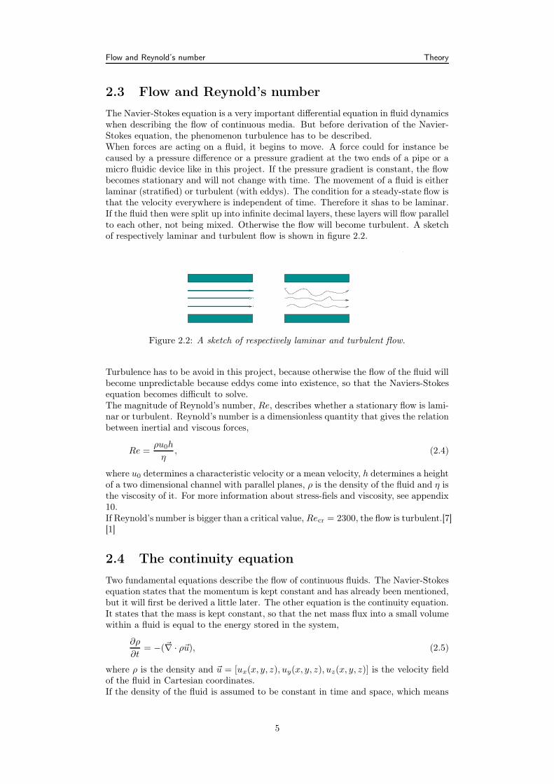
The Navier-Stokes equation is a very important differential equation in fluid dynamicswhen describing the flow of continuous media. But before derivation of the Navier-Stokes equation, the phenomenon turbulence has to be described.When forces are acting on a fluid, it begins to move. A force could for instance becaused by a pressure difference or a pressure gradient at the two ends of a pipe or amicro fluidic device like in this project. If the pressure gradient is constant, the flowbecomes stationary and will not change with time. The movement of a fluid is eitherlaminar (stratified) or turbulent (with eddys). The condition for a steady-state flow isthat the velocity everywhere is independent of time. Therefore it shas to be laminar.If the fluid then were split up into infinite decimal layers, these layers will flow parallelto each other, not being mixed. Otherwise the flow will become turbulent. A sketchof respectively laminar and turbulent flow is shown in figure 2.2.
Figure 2.2: A sketch of respectively laminar and turbulent flow.
Turbulence has to be avoid in this project, because otherwise the flow of the fluid willbecome unpredictable because eddys come into existence, so that the Naviers-Stokesequation becomes difficult to solve.The magnitude of Reynold’s number, Re, describes whether a stationary flow is lami-nar or turbulent. Reynold’s number is a dimensionless quantity that gives the relationbetween inertial and viscous forces,
Re =ρu0h
η, (2.4)
where u0 determines a characteristic velocity or a mean velocity, h determines a heightof a two dimensional channel with parallel planes, ρ is the density of the fluid and η isthe viscosity of it. For more information about stress-fiels and viscosity, see appendix10.If Reynold’s number is bigger than a critical value, Recr = 2300, the flow is turbulent.[7][1]
2.4 The continuity equation
Two fundamental equations describe the flow of continuous fluids. The Navier-Stokesequation states that the momentum is kept constant and has already been mentioned,but it will first be derived a little later. The other equation is the continuity equation.It states that the mass is kept constant, so that the net mass flux into a small volumewithin a fluid is equal to the energy stored in the system,
∂ρ
∂t= −(~∇ · ρ~u), (2.5)
where ρ is the density and ~u = [ux(x, y, z), uy(x, y, z), uz(x, y, z)] is the velocity fieldof the fluid in Cartesian coordinates.If the density of the fluid is assumed to be constant in time and space, which means
5

Navier-Stokes equation for incompressible fluids Theory
that ∂ρ∂t = 0 and ~∇ρ = 0, then
0 = −(~∇ · ρ~u)m
0 = (~∇ · ρ~u)m
0 = (~∇ρ · ~u) + ρ(~∇ · ~u)m
0 = ~∇~u (2.6)
This very important equation is the continuity equation valid for incompressible fluids.[7]
2.5 Navier-Stokes equation for incompressible fluids
As described in section 2.1, the liquid in this project can be assumed as being in-compressible:Therefores the Navier-Stokes equation for compressible fluids will notbe derivated here.The Navier-Stokes equation for incompressible fluids is Newton’s second law for fluidparticles, and it is compatible with continuous fluids.From classical mechanics Newton’s second law for an ordinary particle with mass minfluenced by external forces
∑
j~Fj has the form
m~a = md~u
dt=∑
j
~Fj . (2.7)
In fluid mechanics it is easier to work with the density, ρ, instead of the mass, m,wherefore the equation is divided by the volume, V . Thus
mV
d~udt =
∑
j
~Fj
Vmρd~u
dt =∑
j~fj , (2.8)
where ~fj is the volume specific force or force density.The velocity in a microscopic space somewhere in the fluid is called the Euler velocity.It means that the velocity for a single fluid particle is a function of time, t, and space,~r, and so the volume specific velocity is written ~u(~r, t).Differentiation with regard to time and summation over all directions in space, rep-resented by i, gives
d~u
dt=
∂~u
∂t+
(
∂
∂tri
)
∂i~u =∂~u
∂t+ vi∂i~u. (2.9)
Thus
d~u
dt=
∂~u
∂t+ (~u · ~∇)~u. (2.10)
Now Newton’s Second law reads∑
j
~fj = ρd~u
dt= ρ
(
∂~u
dt+ (~u · ~∇)~u
)
, (2.11)
The external forces acting on a fluid are the so-called body-forces that has to bedetermined.The force density of the gravitation force, ~g, acting on a fluid can be derived from theexpression from classical mechanics, when divided by the volume, V ,
~Fgrav = m~gm
~Fgrav
V = mV ~g
m~fgrav = ρ~g. (2.12)
6

Navier-Stokes equation for incompressible fluids Theory
The force density of an electrical force acting on a polarized fluid is found in the sameway as the gravity force. Thus
~fel = ρel~E, (2.13)
where ρel is the charge density and ~E is an external electrical field.The force density caused by a pressure is derived by considering a region, Ω, in a fluidand the corresponding surface δΩ with a surface normal vector ~n pointing outwardsperpendicular to it.Using Gauss’s theorem the external force, ~fpres, acting on this region due to thepressure p is given by the surface integral over −~np, beeing the outward force perarea from the region acting on the surroundings,
~Fpres =
∫
δΩ
(−~np)da =
∫
Ω
(~∇p)dr. (2.14)
Now the force density of the pressure acting on the fluid becomes [1]
~fpres = −~∇p. (2.15)
The last force derived here is the viscous force.From an expression for conservation of the monentum, Navier-Stokes equation can bewritten as
ρ(∂t~u + (~u · ~∇)~u) = (~∇ · ~τ ) + ρ~g + ρel~E, (2.16)
where τ is a stress-tensor defined as
τ = −pIij + η(~∇~u + (~∇~u)†) − (2
3η − k)(~∇ · ~u) ~∂ij (2.17)
(~∇~u)† is the transposed of (~∇~u), Iij is the identity matrix, p is the pressure and k is
the thermal conductivity. For incompressible fluids ~∇~u = 0 in accordance with thecontinuity equation and so the last term can be neglected. The stress-tensor can thenbe written on the form
τ = −pIij + η(~∇(~u) + (~∇v)†)m
τ = −pIij − ηγ (2.18)
where γ = ~∇~u + (~∇~u)† is a shear rate-tensor. The first part of the stress-tensor, p~∂,is equivalent to the pressure contribution to an inviscosit fluid, and the second part,ηγ, is the contribution from viscous forces in the fluid.Now an expression for the term (~∇∇τ) in the Navier-Stokes can be derived,
(~∇ · ~τ) = ~∇ · (−pIij + η~γ)m
(~∇ · ~τ) = −~∇ · (pIij) + ~∇ · (η~γ)m
(~∇ · ~τ) = −~∇p + ~∇ · (η(~∇~u + (~∇~u)†))m
(~∇ · ~τ) = −~∇p + ~∇ · (η~∇~u) + ~∇ · (η(~∇~u)†)m
(~∇ · ~τ) = −~∇p + η~∇2~u + ~∇ · (η(~∇~u)†)m
(~∇ · ~τ) = −~∇p + η~∇2~u + η~∇ · (~∇~u)m
(~∇ · ~τ) = −~∇p + η~∇2~u. (2.19)
In the derivation it is used that the identity matrix states that I = 1 when i = j, orotherwise Iij = 0. For derivation of the last part of the equation is it used that the
fluid is incompressible and steady-state and so ~∇ · ~u = 0.
7
Poiseuille flow Theory
In the expression derived, the force density of the pressure force and the force densityof the viscous force is included. The force density and the pressure force is knownfrom equation 2.15. Then the force density of the viscous force becomes [7]
~fvisc = η~∇2~u (2.20)
The sum of all the body-forced is the resulting force written on the right side of theNavier-Stokes equation for a compressible fluid. Therefore the Navier-Stokes equationreads [1]
ρ(∂~u∂t + (~u · ~∇)~u) =
∑
j~fj
mρ(∂~u
∂t ~u + (~u · ~∇)~u) = ρ~g + ρel~E − ~∇p + η~∇2~u. (2.21)
The continuity equation states, that for a steady-state flow ~∇·~u = 0. This expressionenter into the Navier-Stokes that now becomes
0 = ρ~g + ρel~E − ~∇p + η~∇2~u. (2.22)
In this project only the pressure force dencity and the viscous force density have tobe considered. There is no electrical force acting on the fluid, and the gravitationforce and the hydrostatic pressure will cancel each other out. Therefore the first twoterms in the Navier-Stokes equation do not have to be considered. Then, finally, theNavier-Stokes equation that is solved in this project becomes
0 = −~∇p + η~∇2~u. (2.23)
2.6 Poiseuille flow
The Navier-Stokes equation is a nonlinear differential equation. It is difficult to solveanalytically, but in a few cases analytical solutions can be found. One of the casesfor which it is possible to solve the Navier-Stokes equation analytical is for a pressureinduced steady-state flow in an infinity long and translational invariant channel. Thisflow problem is called a Poiseuille flow problem and is very important for this project.On the microscopic level, a no-slip boundary condition is obtained for complete mo-mentum relaxation between the molecules in the fluid and the molecules in the wall,
u(r) = 0, for r ∈ δΩ. (2.24)
In general the no-slip boundary condition for the velocity field is valid for micro fluidicsystems.In a Poiseuille flow problem the fluid is driven through a long straight rigidchannel by imposing a pressure difference between the two ends of the channel.When a fluid is flowing through a channel parallel to the x axis, the channel is assumedto be translation invariant in that direction. The constant cross section in the yzdirection is denoted C, while the boundary is denoted δC. A constant pressuredifference, ∆p, over a segment, L, of the channel is maintained, see figur 2.3. Thenthe boundary conditions for the pressure field becomes
p(0) = p0 + ∆p, (2.25)
p(L) = p0. (2.26)
The gravitational force is eliminated by the hydrostatic pressure gradient in the ver-tical direction and thus it is left out of the analyze.The translation invariance of the channel in the z direction combined with the vanish-ing forces in the yz plane implies that the velocity field is not dependent on x, whilethe only non zero velocity component is in the x direction. This implies that the non-linear term (v · ∆)v in the Navier-Stokes equation is zero. Thus the Navier-Stokesequation becomes
0 = η~∇2ux(y, z)− ~∇p. (2.27)
8

Poiseuille flow Theory
δC
x
yz
p(L) = p0
p(0) = p0 + ∆p
L
C
Figure 2.3: Pouiseuille flow problem in a channel. [1]
As stated earlier the velocity field in the y and z directions are zero. Therefore, theterms δyp and δzp are zero. Consequently the pressure field is only dependent on x.Then the Navier-Stokes equation becomes
η[δ2y + δ2
z ]ux(y, z) = δxp(x). (2.28)
As seen from the equation, the left hand side is a function of y and z while the righthand side is only a function of x. The only solution to this equation is obtained whenboth sides are equal to the same constant.The solution to the right hand side is simple because the constant pressure gradientimplies that the pressure field is a linear function of x, when the boundary conditionsis used to obtain the pressure,
p(r) =∆p
L(L − x) + p0. (2.29)
The obtained result is used in the Navier-Stokes equation to obtain
η[δ2y + δ2
z ]ux(y, z) = −∆pL , for (y, z) ∈ C (2.30)
u(y, z) = 0, for (y, z) ∈ δC (2.31)
When the velocity field is determined, it is possible to determinate the fluid volumedischarge per time, which is also called the flow rate, Q
Q =
∫
c
vx(y, z)dydz. (2.32)
Now, having obtained an expression for the flow rate, Q, the is how far it is possibleto get without specifying the actual shape of the channel.
2.6.1 Cross-sections
In the following sections the flow rate will be calculated for some specific cross-sectionsof the channels.The calculations are important for the experiments, when the flow rate through adevice containing a micro fluidic cooling systems is estimated.
2.6.1.1 Circular cross-section
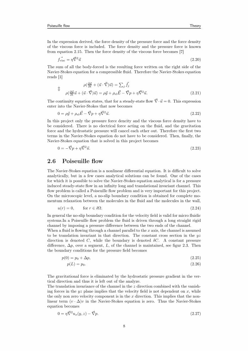
The first cross-section for which the flow rate, Q, now will be derived, is a circularcross-section because all tubes in experimental set-up have a circular cross-section,see figure 2.4.To make the derivation as simple as possible, it is necessary to change the coordi-nate system from Cartesian coordinates to cylindrical coordinates by a coordinate
9
Poiseuille flow Theory
y
x
a
Figure 2.4: Circular cross-section with radius a. [1]
transformation,
(x, y, z) = (x, r cosφ, r sin φ), (2.33)
~ex = ~ex, (2.34)
~er = cosφ~ey + sin φ~ez, (2.35)
~eφ = − sinφ~ey + cosφ~ez, (2.36)
~∇2 = ∂2x + ∂2
r + 1r ∂r + 1
r2 ∂φ. (2.37)
The symmetry reduces the velocity field to ~v = vx(r)~ex. Then the Navier-Stokesequation becomes a second order differential equation,
[δ2r +
1
rδr]ux(r) = −∆p
ηL, (2.38)
The solution to this equation is the solution to the homogeneous differential equationplus a solution to the inhomogeneous equation. The solution to the homogeneousequation has the form vx(r, φ) = A + B ln r. One solution to the inhomogeneousequation is vx(r) = − ∆p
4ηLr2. When the boundary conditions is used, the velocity forthe channel is
ux(r, φ) =∆p
4ηL(a2 − r2). (2.39)
To determine the flow rate, Q, through the system, the velocity is integrated in theequation for the flow rate, which now becomes
Q =
∫ 2π
0
dφ
∫ a
0
∆p
4ηL(a2 − r2) =
π
8
a4
ηL∆pdr. (2.40)
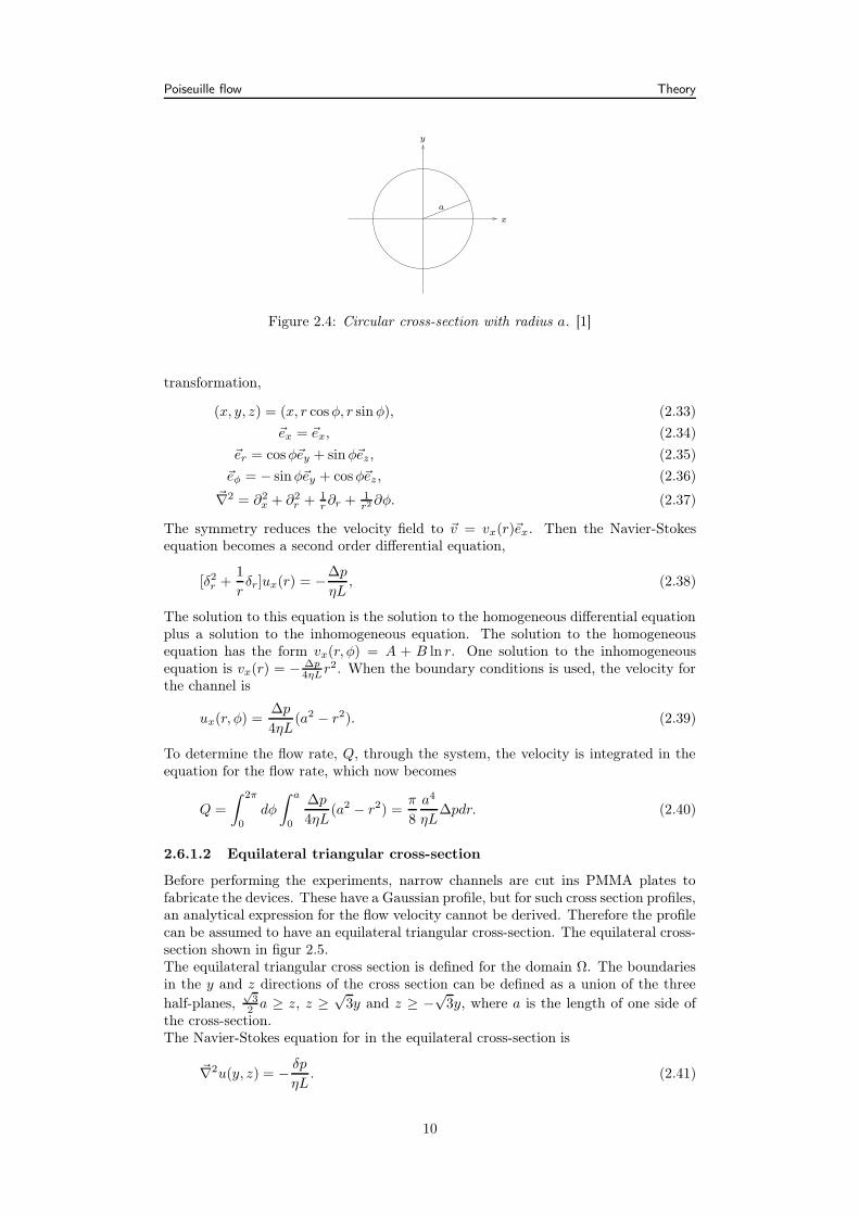
2.6.1.2 Equilateral triangular cross-section
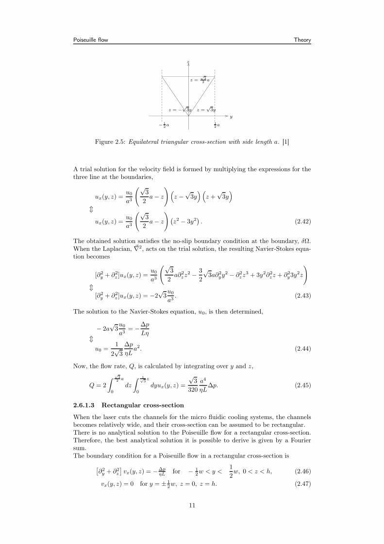
Before performing the experiments, narrow channels are cut ins PMMA plates tofabricate the devices. These have a Gaussian profile, but for such cross section profiles,an analytical expression for the flow velocity cannot be derived. Therefore the profilecan be assumed to have an equilateral triangular cross-section. The equilateral cross-section shown in figur 2.5.The equilateral triangular cross section is defined for the domain Ω. The boundariesin the y and z directions of the cross section can be defined as a union of the three
half-planes,√
32 a ≥ z, z ≥
√3y and z ≥ −
√3y, where a is the length of one side of
the cross-section.The Navier-Stokes equation for in the equilateral cross-section is
~∇2u(y, z) = − δp
ηL. (2.41)
10
Poiseuille flow Theory
− 12a 1
2a
y
z =√
3yz = −√
3y
z =√
32
a
z
Figure 2.5: Equilateral triangular cross-section with side length a. [1]
A trial solution for the velocity field is formed by multiplying the expressions for thethree line at the boundaries,
ux(y, z) =u0
a3
(√3
2a − z
)
(
z −√
3y)(
z +√
3y)
m
ux(y, z) =u0
a3
(√3
2a − z
)
(
z2 − 3y2)
. (2.42)
The obtained solution satisfies the no-slip boundary condition at the boundary, δΩ.When the Laplacian, ~∇2, acts on the trial solution, the resulting Navier-Stokes equa-tion becomes
[∂2y + ∂2
z ]ux(y, z) =u0
a3
(√3
2a∂2
zz2 − 3
2
√3a∂2
yy2 − ∂2zz3 + 3y2∂2
zz + ∂2y3y2z
)
m[∂2
y + ∂2z ]ux(y, z) = −2
√3u0
a3. (2.43)
The solution to the Navier-Stokes equation, u0, is then determined,
− 2a√
3u0
a3= −∆p
Lηm
u0 =1
2√
3
∆p
ηLa2. (2.44)
Now, the flow rate, Q, is calculated by integrating over y and z,
Q = 2
∫
√3
2a
0
dz
∫ 1√3z
0
dyux(y, z) =
√3
320
a4
ηL∆p. (2.45)
2.6.1.3 Rectangular cross-section
When the laser cuts the channels for the micro fluidic cooling systems, the channelsbecomes relatively wide, and their cross-section can be assumed to be rectangular.There is no analytical solution to the Poiseuille flow for a rectangular cross-section.Therefore, the best analytical solution it is possible to derive is given by a Fouriersum.The boundary condition for a Poiseuille flow in a rectangular cross-section is
[
∂2y + ∂2
z
]
vx(y, z) = −∆pηL for − 1
2w < y <1
2w, 0 < z < h, (2.46)
vx(y, z) = 0 for y = ± 12w, z = 0, z = h. (2.47)
11

Hydraulic resistance Theory
z
y0
h
− 12w 1
2w
Figure 2.6: Rectangular cross-section with height h and width w. [1]
The velocity field for a Poiseuille flow in a rectangular channel is
vx(y, z) =4h2∆p
π3ηL
∞∑
n,odd
1
n3
[
1 − cosh(
nπ yh
)
cosh(
nπ w2h
)
]
sin(
nπz
h
)
. (2.48)
The flow rate for a rectangular channel can be fund by solving the integral in equation2.32. Then it can be obtained that obtain
Q =8h3w∆p
π4ηL
∞∑
n,odd
[
1
n4− 2h
πw
1
n5tanh
(
nπw
2h
)
]
. (2.49)
2.7 Hydraulic resistance
As obtained in the previous sections, a constant pressure drop, ∆p, will result in aconstant flow rate, Q, This connection is is described by the Hagen-Poiseuille law thatstates
∆p = RhydQ, (2.50)
where Rhyd is the hydraulic resistance. The hydraulic resistance for the three cross-section described above can directly be derived from the expressions of flow rates, Q.The hydraulic resistance of the three described cross-sections is written in table ??.The hydraulic resistance for the rectangular cross-section is an approximated result.
Cross-section Rhyd
Circle 8πηL 1
a4
Equilateral triangular 320√3ηL 1
a4
Rectangle 12ηL1−0.63(h/w)
1h3w
Table 2.1: Hydraulic resistance of different cross-sections
2.7.1 Two straight channels
When two straight channels are connected to form one long channel, the expressionsfor an ideal Poiseuille flow is no longer valid. However, when the non-linear term inthe Navier-stokes equation is insignificant small, the flow rate can be approximated bya Poiseuille flow. The magnitude of the no-linear term in the Navier-stokes equationthen corresponds to Reynold’s number, Re.
2.7.1.1 Two straight channels in series
When to channels are connected in series, the Hagen-Poiseuille law is approximatelyvalid after the channels are connected. This is equivalent to that Reynold’s number,
12

Conduction and convection Theory
Re, is low, and the channels are long. It this case the total hydraulic resistancebecomes
Rhyd total = Rhyd 1 + Rhyd 2, (2.51)
where Rhyd 1 and Rhyd 2 are the hydraulic resistance of respectively the first channeland the second channel.
2.7.1.2 Two straight channels in parallel
When two channels are connected in parallel, and it is assumed that Reynold’s num-ber, Re, is small and the channels are long, the Hagen-Poiseuille law is approxiatelyvalid. The flow in the channels are conserved, Qtotal = Q1 + Q2, and thus the totalhydraulic resistance becomes [1].
Rhyd total =
(
1
Rhyd 1+
1
Rhyd 2
)−1
. (2.52)
2.8 Conduction and convection
The physical property that describes the rate at which a material is conducting heat, isthe thermal conductivity, k. A high thermal conductivity results in a high conductionof heat, and a low thermal conductivity results in a low conduction of heat. [20]There are basically three ways of heat conduction which is conduction, convectionand radiation. Conduction in fluids can be described as molecular energy transportand happens, when an energy transporting molecule moving with a high velocity hitsa molecule moving with a lower velocity. Then the first molecule will transfer some ofits energy to the second molecule. Thereby the velocity of the slow moving moleculeis accelerated and velocity of the fast moving molecule is slowed.Heat transfer by convection happens when heat is transported by the bulk motion ofa fluid, that thereby is carrying heat with it.Heat conduction by radiation happens when electromagnetic waves are emitted by ahot object and thereby carrying energy away from the object. [21]In a microfluidic cooling system the heat is transferred by conduction and convection,and therefore these two ways of heat conduction will be described in details below.
2.8.1 Conduction
Conduction is described by the heat equation. The heat equation can be derived froman expression of energy conservation in a small element of a system, because the heatconducted into the element, Qconducted in, and the heat generated within the element,Q, are equal to the heat conducted out of the element, Qconducted out, and the changein energy stored in the element, ∂ε
∂t . Thus
Qconducted in + Q = Qconducted out +∂ε
∂t. (2.53)
If the heat conduced into the element is subtracted from the heat conducted out ofthe element, the amount is equal to the change in energy conducted out of the system,which is also the change in the heat flux vector, ~q. Combining this with the equationabove it results in
~∇~q = Q − ∂ε
∂t. (2.54)
The heat flux vector, ~q, is given by Fouier’s law, which states that
~q = −k~∇T, (2.55)
13

Conduction and convection Theory
where k is the thermal conductivity and T is the temperature. This equation describesthe molecular transport of heat in an isotropic material. An isotropic material is amaterial that has no preferred directions, so that the heat is conducted with the samethermal conductivity, k, in all directions.The energy stored in the element is equal to the thermal energy,
∂ε
∂t= ρC
∂T
∂t(2.56)
where C is the heat capacity.If equation 2.54, equation 2.55 and equation 2.56 are combined, the heat equationbecomes
~∇(−k~∇T ) = Q − ρC∂T
∂t: HydraulicResistanceofdifferentcross− sections.s
(2.57)m
ρC∂T
∂t+ ~∇(−k~∇T ) = Q. (2.58)
For the steady-state solution the time dependent part of the heat equation is zero,∂T∂t = 0, wherefore for steady state the heat equation becomes
~∇(−k~∇)T = Q. (2.59)
This is the equation FEMLab is using when the calculations is carried out. [23] [24]
2.8.2 Convection
Heat transfer will occur between a solid and a fluid in motion, when there is a tem-perature difference between them. When the fluid is in motion, the dominating heattransportation happens by convection, which will be described further in section ??.If the temperature of a solid induces a fluid to move, the phenomenon is know asnatural convection. Natural convection is a strong function of the temperature differ-ence.If the solid is cooled by a fluid in motion, it is know as forced convection. [23]When convection is considered in the heat equation, an amount of energy has to besubtracted from the heat equation, because it is transported away by the fluid anddoes not heat the system. The amount of energy is equal to
∆εtransported = ρC~u~∇T. (2.60)
Including this expression in the heat equation results in
ρC∂T
∂t+ ~∇(−k~∇T ) = Q − ρC~u~∇T. (2.61)
∆εtramsported is subtracted from Q because this amount of energy does not heat thesystem.It is assumed that the fluid is incompressible, ~∇ · ~u = 0.For a steady state system the time dependent part of the equation is zero, and there-fore the time independent heat equation with the convection term becomes
ρC~u~∇T + ~∇(−k~∇T ) = Q. (2.62)
2.8.3 Boundary conditions
Based on equation 2.62 the boundary conditions for the microfluidic system can becalculated.
14

The Péclet number Theory
At the outer boundary the system is thermically isolated from the surroundings, sothat the boundary condition becomes
~n ·(
−k~∇T + ρc~uT)
= 0, (2.63)
where ~n is a normal vector perpendicular to the boundary.At the inlet, the water flowing into the micro fluidic cooling system with a constanttemperature. Thus the boundary condition is
T = T0, (2.64)
where T0 is a constant temperature.At the outlet the boundary condition becomes
n ·(
−k~∇T)
= 0. (2.65)
When the last boundary condition is used there is no conduction perpendicular tothe boundary. Thus, there is only convection on the other side of the boundary.
2.9 The Péclet number
The Péclet number, Pe, is a quantity used when describing the micro fluidic coolingsystems and can be used in calculations involving convective heat transfer. It is adimensionless number that gives the ratio between convection and conduction, seesection 2.8.The Péclet number is defined as
Pe =u0ρCL
k, (2.66)
where ρ is the density of the fluid flowing in a channel, C is the heat capacity, k is thethermal conductivity, u0 is the mean velocity refering to a characteristic velocity scaleand L states a characteristic length scale, for instance the height of the channels.If Pe is small, Pe 1, conduction is important, because the velocity of the fluidis very small. If, on the other hand, Pe er big, Pe 10, then convection becomesimportant.For a derivation of the Péclet number, see appendix 12.
15
Chapter 3
Numerical simulations involving
FEMLab
The examples of poiseuille flows and convection-diffusion described previous are veryimportant in fluid mechanich. However, it is only possible to solve partial differentialequations like Navier-Stoke’s equation and the heat equation analytical in special andrelatively simple cases with highly symmetry. The micro fluidic cooling systems stud-ied in this project are fairly complex micro fluidic problems. Therefore it is necessaryto perform numerical simulations to get solutions to the complicated partiel differen-tial equations, that appear in the calculations.In this project the equations are solved to optimize the systems using the nume-rical solver program FEMLab, witch is working by using MatLab, that transformsthe problems into matrix problems. FEMLab performs a high-level programminglanguage implementation of nonlinear topology optimization based on the MatLabprogramming language, and it is able to solve fairly complex microfluidic problemsinvolving for instance the Navier-Stokes equation and the heat equation relativelyuncomplicated. FEMLab is using a finite element method, FEM, which is very goodfor fluidic systems with a low Reynolds number, not exhibiting turbulence. [1]
3.1 The finime element method, FEM
The finite element method, FEM, approximates a problem involving partial dif-ferential equations with a problem having a finite number of unknown parametersby introduction of finite elements describing the possible form of the approximatesolution. Thereby FEMLab performs a discretization of the original problem.The starting point for the FEM method is a mesh, splitting up the geometry of theproblem into small triangular units of the same shape. When performing the finalelement method, equation will only be solved in the mesh points, called the meshvertices, which are the corners of the triagular units, and the equation will be ap-proximated between the points. Therefore, the greater the number of mesh pointsdefined, the greater the accuracy of the calculations will be. [15]The finite element method, FEM, will not be described here, because it is not ne-cessary to understand in order to run the FEMLab and MatLab programming code.The fundamental MatLab scripts used to perform the topology optimization of themicro fluidic cooling systems were written before the project began. These have mostof all been used as a tool, and only a few changes have been made within them. Incontrast, the design of the cooling systems and the physical constants were stated byuse if the graphical user interface in FEMLab.
16
The MMA topology optimization method Numerical simulations involving FEMLab
3.2 The MMA topology optimization method
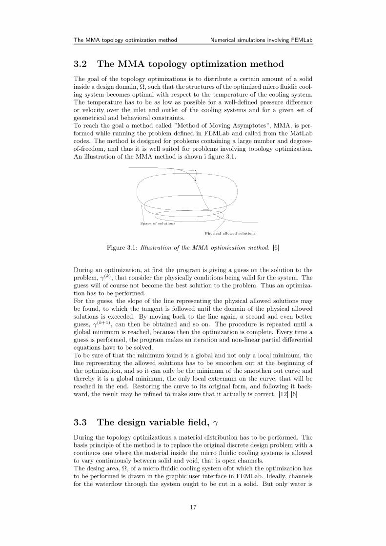
The goal of the topology optimizations is to distribute a certain amount of a solidinside a design domain, Ω, such that the structures of the optimized micro fluidic cool-ing system becomes optimal with respect to the temperature of the cooling system.The temperature has to be as low as possible for a well-defined pressure differenceor velocity over the inlet and outlet of the cooling systems and for a given set ofgeometrical and behavioral constraints.To reach the goal a method called "Method of Moving Asymptotes", MMA, is per-formed while running the problem defined in FEMLab and called from the MatLabcodes. The method is designed for problems containing a large number and degrees-of-freedom, and thus it is well suited for problems involving topology optimization.An illustration of the MMA method is shown i figure 3.1.
Physical allowed solutions
Space of solutions
Figure 3.1: Illustration of the MMA optimization method. [6]
During an optimization, at first the program is giving a guess on the solution to theproblem, γ(k), that consider the physically conditions being valid for the system. Theguess will of course not become the best solution to the problem. Thus an optimiza-tion has to be performed.For the guess, the slope of the line representing the physical allowed solutions maybe found, to which the tangent is followed until the domain of the physical allowedsolutions is exceeded. By moving back to the line again, a second and even betterguess, γ(k+1), can then be obtained and so on. The procedure is repeated until aglobal minimum is reached, because then the optimization is complete. Every time aguess is performed, the program makes an iteration and non-linear partial differentialequations have to be solved.To be sure of that the minimum found is a global and not only a local minimum, theline representing the allowed solutions has to be smoothen out at the beginning ofthe optimization, and so it can only be the minimum of the smoothen out curve andthereby it is a global minimum, the only local extremum on the curve, that will bereached in the end. Restoring the curve to its original form, and following it back-ward, the result may be refined to make sure that it actually is correct. [12] [6]
3.3 The design variable field, γ
During the topology optimizations a material distribution has to be performed. Thebasis principle of the method is to replace the original discrete design problem with acontinuos one where the material inside the micro fluidic cooling systems is allowedto vary continuously between solid and void, that is open channels.The desing area, Ω, of a micro fluidic cooling system ofot which the optimization hasto be performed is drawn in the graphic user interface in FEMLab. Ideally, channelsfor the waterflow through the system ought to be cut in a solid. But only water is
17

The Darcy force Numerical simulations involving FEMLab
considered in the system. Therefore, in the beginning, the area of the cooling sys-tem can be assumed to be filled with a sponge, because that kind of material eitherconsists of solid or empty holes, in which water is able to flow. The sponge can beassumed as being a porous idealized material of spatial varying permeability in thedesign domain, Ω, where solid walls correspond to the limits of very low permeability,and open channels correspond to the limit of very high permeability. Thus, duringthe optimization, it is the amount of moving water and the amount of stationarywater that will change. For the micro fluidic cooling systems is corresponding to therelationship between channels and walls. To define this relationship a design variablefield, γ, that defines where the water is moving and where it is stationary. γ can alsobe assumed to control the local permeability of the medium. For γ at respectivelythe wall and open channels holds
Walls: γ = 0Open channels: γ = 1
When the topology optimization is completed, there will be either walls or openchannels at each of the points defined for the design area of the micro fluidic cool-ing systems, and γ will only take the values γ = 0 or γ = 1, respectively. Any-way, smeared-out gray-scales will appear at the boundaries of the topology optimizedstructures, it what areas there will be neither empty channels nor walls, which isnot in agreement with the conditions established for the optimizations. Afterall, thesmeared-out gray-scales appear because MatLab and FEMLab are performing num-merical optimizations, and thus the result will never be exact.It was described above that only water is considered to appear the system. Thereforethe so-called walls of the system actually is stationary water, so that the results of theoptimizations are not physically correct, because the walls in fact consist of a solidhaving other material parameters than the water. Anyway, the assumption with sta-tionary water is a reasonable approximation to reality, and it makes the optimizationsrelatively simple. [6] [12]
3.4 The Darcy force
Darcy’s law states that when water is flowing through a micro fluidic cooling system,that can be described as a sponge as described in section 3.3, it is influenced by africtional force, the so-called Darcy force, ~fDarcy, which is given by
~fDarcy = −α~u, (3.1)
where ~u is the velocity of the water, and α is the inverse of the local permeabilityof the system at a certain point. α is dependent on the relationship between thewalls and the open channels in the micro fluidic cooling systems. Equation 3.1 isonly approximately valid for a porous media, but because only solids wall and openchannel are assumed to be represented for the final structure, the equation can beused. Therefore, the equation can be used in the calculations.For a distinct point of the cooling system, α can be written as a function of the designvariable field, γ, by convex interpolation,
αγ = αmin + (αmax − αmin)q(1 − γ)
q + γfor γ ∈ [0; 1], (3.2)
where q is a real and positive design variable function due to tune the shape of γ.q is important for the structures of the micro fluidic cooling systems when these aretopology optimized. If the variale functin q is increased in the MatLab code some ofthe problems with smeared-out gray-scale structures may disappear.To write up the equation for αγ, it was assumed that α = αmin, when the collingsystem is not containing any solid (or stationary water), and α = αmax, when the
18

The objective function, φ, and specific geometry Numerical simulations involving FEMLab
system is completely filled with a solid. For water flowing in a two dimensional channelit is assumed that αmin = 0. On the other hand, when the system is completely filledwith a solid, water is unable to flow through it and so αmax = ∞. However, theFEMLab and MatLab program is unabble when performing numerical calculationinvolving the number infinity. Thus αmax is have to be a very high number, becausethe Darcy number, Da, is established to be Da = 1 · 10−5 in the program.Darcy’s number, Da, is a dimensionless number that states the relationship betweenviscous and porous friction forces. Darcy’s number is proportioale to the Darcy force.
Da =η
αmaxl2(3.3)
mαmax =
η
Da · l2 , (3.4)
where l is a characteristic length scale of the system and u is a caratheristic velocity.Darcy’s number has an influence on the structures of the optimized cooling systems.[12] [6]
3.5 The objective function, φ, and specific geometry
The FEMLab and MatLab program is optimizing a objective function, φ(~u, γ), which,generally, in FEMLab is defined as
φ(~u, γ) =
∫
Ω
A(~u, γ)d~r +
∫
∂Ω
B(~u, γ)d~s +∑
∂2Ω
C(~u, γ). (3.5)
For the objective function the first term corresponds to the design area, Ω, of thedefined micro fluidic cooling system, the second term corresponds to the boundariesof the geometri, ∂Ω, and the third term corresponds to defined points, ∂2Ω, withinthe geometry. [12] [6]During the optimizations a value for A is the only one term that is defined, becausethe optimizations have to be performed on the whole area of the micro fluidic coolingsystem. B = 0 and C = 0, and so
φ(~u, γ) =
∫
Ω
A(~u, γ)d~r. (3.6)
From the objective function the average temperature, T , of the optimized micro fluidiccooling systems can be derived when dividing by the area, Acooler, of it,
T =φ(~u, γ)
Acooler. (3.7)
During the optimization, φ is always miminized, so that A = T . In this way thetemperature, T , of the design region, Ω, is minimized.
19

Chapter 4
Set-up for topology
optimization problems using
FEMLab
The topology optimization problems are solved using a numerical solver programsFEMLab and MatLab. Starting FEMLab from MatLab makes is possible to defineand perform calculations on complicated topology optimization problems.The geometry of the problems and the physical parameters for the problems aredefined in the FEMLab graphical user interface, GUI, and associated MatLab pro-grammes are used to solve the topology optimization problems.
4.0.1 The Navier-Stokes application mode, geometry and mesh
When starting FEMLab, "Fluid Dynamic" is chosen for a two dimensional problem.Then it is chosen that is it an "Incompressible Navier-Stokes" equation that has tobe solve for "Steady-State Analyses", because the water flowing in the channels isassumed to be steady-state as described in section 2.1. Now it is possible to solveproblems involving liquids or gases in motion.The geometry of the problem is defined in two dimensions in the FEMLab GUI. Thegeometry is separated into different parts to have the central design region definedbesides the inlet and outlet for the system. When performing the simulations, allphysical parameters have to be defined in SI-units, and thus the lengths defined forthe structure is in meter.The choose of mesh is important for the stability and the accuracy of the numericalobtained results. The mesh for the difference parts of a structure is defined in "Sub-domains" under "Mesh Parameters" in the menu "Mesh". In the design region of themicro fluidic cooling systems a fine mesh is defined, while for the inlet and outlet acoarser mesh is drawn.The "Incompressible Navier-Stokes" application mode solves the Navier-Stokes prob-lem for the pressure for the velocity vector components appearing in the equation.Navier-Stokes equation, not including the electrical force density, and the continuityequation for an incompressible, steady-state fluid are
~F = ρ∂~u∂t − η ~∇2~u + ρ(~u) · ~∇)~u + ~∇p (4.1)
~∇~u = 0, (4.2)
where ~F is the total force or volume force, p is the pressure, ~u is the velocity of theliquid flowing in the system, η is the viscosity of it and ρ is the density of it.FEMLab uses a generalized version of the Navier-Stokes equation in terms of transport
20
Set-up for topology optimization problems using FEMLab
properties and velocity gradients. Starting with the momentum balance in terms ofstresses and inserting an expression for the viscous stress tensor, τvisc = η( ~∇~u + ( ~∇~u)T ),the equation becomes
~F = ρ∂~u∂t − ~∇(η(~∇~u + (~∇~u)†) + ρ(~u) · ~∇)~u + ~∇~p (4.3)
~∇~u = 0. (4.4)
An expression for the viscous stress tensor, η(~∇~u + ( ~∇~u)T ), witch is the second part
of the total stress tensor, τ = −p ~Iij + η(~∇(~u) + (~∇v)T ), see section 2.5, is inserted inthe equation to obtain the form of the Navier-Stokes equation used in the FEMLab"Subdomain Settings",
ρ(~u · ~∇)~u = ~∇ · (−p · Iij + η(~∇~u + (~∇~u)†)) + ~F (4.5)
~∇~u = 0 (4.6)
In the dialog box for "Subdomain Setting" under "Physics" the parameters of theliquid flowing in the system is defined. Water is used in this project, and thus thephysical parameters are ρ = 1000 kg/m3 and η = 0.001 mPa·s. The gravitation forceand the hydrostatic pressure will cancel each other out and thus the volume force~F = (Fx, Fy) = 0.In "Boundary Settings" under "Physics" the properties for the boundary conditionsof the Navier-Stokes equation is determined. The boundaries for both the inlet andthe outlet has the property "Normal flow/Pressure", because the water is flowingstraight out of the channel, so that the components of the velocity perpendicular tothe water flow is zero.To drive the water through the system, for the inlet and the outlet the pressure isdefined to be p0 = dp and p0 = 0, respectivily.It is also possible to set a velocity of the water flowing into the system. Then forthe inlet a boundary condition "Inflow/Outflow velocity" is chosen in "BoundarySettings", while for the outlet "Pressure" with p0 = 0 is still chosen. The wateris flowing in the x direction, u, and the velocity profile for the inlet is a parabolicfunction defined as
u = s(1 − s)6u, (4.7)
where s is a function defined by FEMLab, that changes between 0 and 1 within thesimulations. The velocity in the y direction, v, is zero. Thus v = 0.For the boundaries surrounding the system, the boundary condition is "No Slip",because the liquid is always stationary at the boundaries. Thus ~u = 0.For the boundaries within the structure it does not make sense to have boundaryconditions. Therefore these are defined to be "Neutral" as if there were no boundaries.[19]
4.0.2 The conduction and convection application mode
The conduction and convection application mode in FEMLab included heat transferby conduction and heat transfer by convection. Is is added to the problem by choosing"Convection and Conduction" in the application mode "Heat Transfer".In FEMLab the nonconservative formulation for the heat equation is used,
ρc∂T
∂t+ ~∇ · (−k~∇T ) = Q − ρc~u · ~∇T, (4.8)
where c is the heat capacitance, T is the temperature, k is the thermal conductivityand Q is the heat added to the system. The fluid is assumed to be incompressibleand steady-state. Thus ∂T
∂t = 0. Then the equation becomes
~∇ · (−k~∇T ) = Q − ρc~u · ~∇T. (4.9)
21
Set-up for topology optimization problems using FEMLab
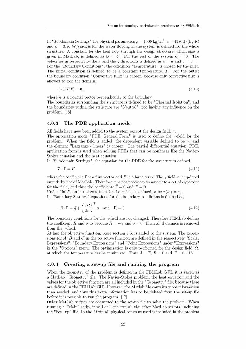
In "Subdomain Settings" the physical parameters ρ = 1000 kg/m3, c = 4180 J/(kg·K)and k = 0.56 W/(m·K)s for the water flowing in the system is defined for the wholestructure. A constant for the heat flow through the design structure, which size isgiven in MatLab, is defined as Q = Q. For the rest of the system Q = 0. Thevelocities in respectivily the x and the y directions is defined as u = u and v = v.For the "Boundary Conditions", the condition "Temperature" is chosen for the inlet.The initial condition is defined to be a constant temperature, T . For the outletthe boundary condition "Convective Flux" is chosen, because only convective flux isallowed to exit the domain,
~n · (k~∇T ) = 0, (4.10)
where ~n is a normal vector perpendicular to the boundary.The boundaries surrounding the structure is defined to be "Thermal Isolation", andthe boundaries within the structure are "Neutral", not having any influence on theproblem. [18]
4.0.3 The PDE application mode
All fields have now been added to the system except the design field, γ.The application mode "PDE, General Form" is used to define the γ-field for theproblem. When the field is added, the dependent variable defined to be γ, andthe element "Lagrange - linear" is chosen. The partial differential equation, PDE,application form is used when solving PDEs that can be nonlinear like the Navier-Stokes equation and the heat equation.In "Subdomain Settings", the equation for the PDE for the structure is defined,
~∇ · ~Γ = F (4.11)
where the coefficient Γ is a flux vector and F is a force term. The γ-field is is updatedoutside by use of MatLab. Therefore it is not necessary to associate a set of equationsfor the field, and thus the coefficients ~Γ = 0 and F = 0.Under "Init", an initial condition for the γ field is defined to be γ(t0) = γ0.In "Boundary Settings" equations for the boundary conditions is defined as,
−~n · ~Γ = ~g +
(
δR
δv
)T
µ and R = 0 (4.12)
The boundary conditions for the γ-field are not changed. Therefore FEMLab definesthe coefficient R and g to become R = −γ and g = 0. Then all dynamics is removedfrom the γ-field.At last the objective function, φ,see section 3.5, is added to the system. The expres-sions for A, B and C in the objective function are defined in the respectively "ScalarExpressions", "Boundary Expressions" and "Point Expressions" under "Expressions"in the "Options" menu. The optimization is only performed for the design field, Ω,at which the temperature has be minimized. Thus A = T , B = 0 and C = 0. [16]
4.0.4 Creating a set-up file and running the program
When the geometry of the problem is defined in the FEMLab GUI, it is saved asa MatLab "Geometry" file. The Navier-Stokes problem, the heat equation and thevalues for the objective function are all included in the "Geometry" file, because theseare defined in the FEMLab GUI. However, the Matlab file contains more informationthan needed, and thus this extra information has to be deleted from the set-up filebefore it is possible to run the program. [17]Other MatLab scripts are connected to the set-up file to solve the problem. Whenrunning a "Main" scrip, it will call and run all the other MatLab scripts, includingthe "Set_up" file. In the Main all physical constant used is included in the problem
22

Set-up for topology optimization problems using FEMLab
and defined as FEMLab constants, and the pressure difference over the system or ainitial velocity for the inlet is defined.In the MatLab script "GammaOn" the Darcy force is added to the Navier-Stokesproblem, and the design field, γ is included. By use of the scripts "Solve" and "mma-sub" the whole problem is solve and the resulting design field, γ, the change in γ foreach interaction, the velocity field and finally the temperature field is showed on thescreen by use of the scrip "Plot_Res".
23
Chapter 5
Computer simulations
5.0.5 Simulations
In this section the FEMLab simulations are described. The FEMLab simulations arecarried out in order to determine the optimal temperature over the final micro fluidiccooling systems for a given pressure difference over the inlet and outlet.In the simulations, a pressure difference is defined over the inlet and outlet of thedevice, but a velocity profile could also have been defined. However, this is not donebecause a velocity profile would result in thinner channels within the design structure,which would be very difficult to cut with the laser. Fabrication of the micro fluidiccooling systems is described in section 6.1.
5.0.6 Determination of a global minimum
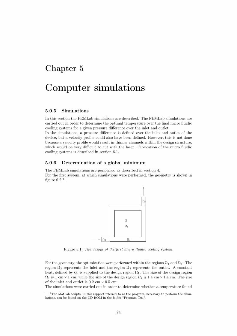
The FEMLab simulations are performed as described in section 4.For the first system, at which simulations were performed, the geometry is shown infigure 6.2 1.
Ω1
Q
Ω4Ω2
Ω3
Figure 5.1: The design of the first micro fluidic cooling system.
For the geometry, the optimization were performed within the regions Ω1 and Ω4. Theregion Ω2 represents the inlet and the region Ω3 represents the outlet. A constantheat, defined by Q, is supplied to the design region Ω1. The size of the design regionΩ1 is 1 cm× 1 cm, while the size of the design region Ω4 is 1.4 cm× 1.4 cm. The sizeof the inlet and outlet is 0.2 cm × 0.5 cm.The simulations were carried out in order to determine whether a temperature found
1The MatLab scripts, in this rapport referred to as the program, necessary to perform the simu-lations, can be found on the CD-ROM in the folder "Program T01".
24

Computer simulations
for an optimized structure was a minimum temperature or not. To do so, the temper-ature measured from the optimization was compared to the temperature of anotheroptimized structure, for which the pressure difference over the inlet and outlet wasnot the same. Thus further simulations were carried out for the same geometry, butfor other pressures differences between 0.033 Pa and 2 Pa over the inlet and outlet. 2
The material parameter, γ0, is set equal to 0.95. Thereby there has to be at least 5%material within the design structure for which the optimixations are performed. Theprogram can choose how much material the structure contains, when performing theoptimizations.The optimized structure of the optimal systems is shown in figure 5.2.
Figure 5.2: Optimzed stucture for the micro fluidic cooling system shown in figure 6.2optimized for different pressure differences.
After an optimal stucture for a micro fluidic cooling system is determined, the pres-sure difference over the inlet and outlet is changed, and a new average temperature iscalculated for the new pressure, 3. The obtained temperature is plotted as functionof the pressure, see figure 5.3 4.As noted from figure 5.3, the system that is optimized for a given pressure is notoptimal, because none of the curves has a minimum.The simulations was carried out for many different pressure differences and each timethe obtained result was the same, it was not possible to get an optimized structure.Therefore, it was revealed that the parameters in the program used by the MMAsubroutine to calculate the geometry of the optimal stucture was not correct. The reasonfor this was, that The MMAsub routine needs four variables to carry out an opti-mization. The first variable is f = Φ
Φ0, where Φ is the objective function and Φ0 is a
2The MatLab program for which the geometry is defined is showed in the appendix on the CD-ROM in the folder "Program T01", and the MatLab script for the Main program for differentpressures is shown in the in appendix on the CD-ROM in the folder "Program T01".
3The MatLab scripts, in which the variation of the pressure and the average temperature iscalculated, is shown in the appendix on the CD-ROM in the folder "Plot programs"
4The MatLab script plotting the temperature as a function of the pressure can be found on theCD-ROM in the folder "Plot programs".
25
Computer simulations
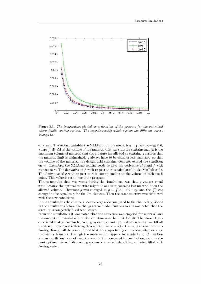
Figure 5.3: The temperature plotted as a function of the pressure for the optimizedmicro fluidic cooling system. The legends specify which system the different curvesbelongs to.
constant. The second variable, the MMAsub routine needs, is g =∫
|A| ·dA−γ0 ≤ 0,where
∫
|A| ·dA is the volume of the material that the stucture contains and γ0 is themaximum volume of material that the stucture are allowed to contain. g ensures thatthe material limit is maintained. g always have to be equal or less than zero, so thatthe volume of the material, the design field contains, does not exceed the conditionon γ0. Therefore, the MMAsub routine needs to have the derivative of g and f withrespect to γ. The derivative of f with respect to γ is calculated in the MatLab code.The derivative of g with respect to γ is correspomding to the volume of each meshpoint. This value is set to one inthe program.The assumption that was wrong during the simulations, was that g was set equalzero, because the optimal stucture might be one that contains less material then theallowed volume. Therefore g was changed to g =
∫
|A| · dA − γ0 and the dgdγ was
changed to be equal to γ for the i’te element. Then the same stucture was simulatedwith the new conditions.In the simulations the channels became very wide compared to the channels optionedin the simulations before the changes were made. Furthermore it was noted that thestucture is completely filled with water.From the simulations it was noted that the structure was emptied for material andthe amount of material within the structure was the limit for γ0. Therefore, it wasconcluded that micro fluidic cooling system is most optimal when water can fill allthe structure, when it is flowing through it. The reason for this is, that when water isflowing through all the stucture, the heat is transported by convection, whereas whenthe heat is transport through the material, it happens by conduction. Convectionis a more efficient way of heat transportation compared to conduction, as thus themost optimal micro fluidic cooling system is obtained when it is completely filled withflowing water.
26
Computer simulations
5.0.7 Changes of the design variable field, γ
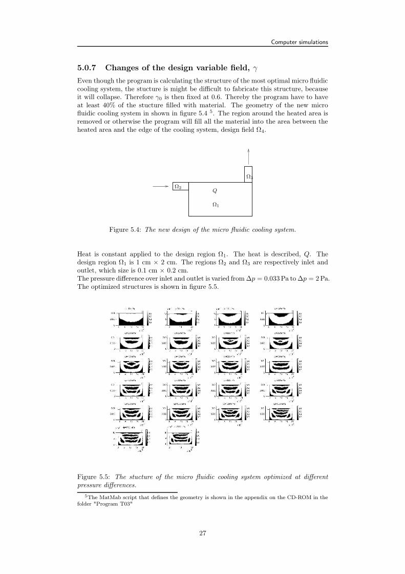
Even though the program is calculating the structure of the most optimal micro fluidiccooling system, the stucture is might be difficult to fabricate this structure, becauseit will collapse. Therefore γ0 is then fixed at 0.6. Thereby the program have to haveat least 40% of the stucture filled with material. The geometry of the new microfluidic cooling system in shown in figure 5.4 5. The region around the heated area isremoved or otherwise the program will fill all the material into the area between theheated area and the edge of the cooling system, design field Ω4.
Q
Ω1
Ω2
Ω3
Figure 5.4: The new design of the micro fluidic cooling system.
Heat is constant applied to the design region Ω1. The heat is described, Q. Thedesign region Ω1 is 1 cm × 2 cm. The regions Ω2 and Ω3 are respectively inlet andoutlet, which size is 0.1 cm × 0.2 cm.The pressure difference over inlet and outlet is varied from ∆p = 0.033 Pa to ∆p = 2 Pa.The optimized structures is shown in figure 5.5.
Figure 5.5: The stucture of the micro fluidic cooling system optimized at differentpressure differences.
5The MatMab script that defines the geometry is shown in the appendix on the CD-ROM in thefolder "Program T03"
27
Computer simulations
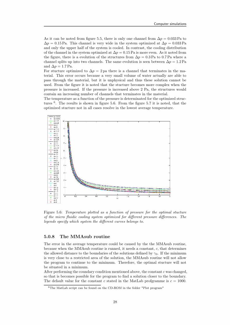
As it can be noted from figure 5.5, there is only one channel from ∆p = 0.033 Pa to∆p = 0.15 Pa. This channel is very wide in the system optimized at ∆p = 0.033 Paand only the upper half of the system is cooled. In contrast, the cooling distributionof the channel in the system optimized at ∆p = 0.15 Pa is more even. As it noted fromthe figure, there is a evolution of the structures from ∆p = 0.3 Pa to 0.7 Pa where achannel splits up into two channels. The same evolution is seen between ∆p = 1.2 Paand ∆p = 1.7 Pa.For stucture optimized to ∆p = 2 pa there is a channel that terminates in the ma-terial. This error occurs because a very small volume of water actually are able topass through the material, but it is unphysical and thus these solution cannot beused. From the figure it is noted that the stucture becomes more complex when thepressure is increased. If the pressure is increased above 2 Pa, the structures wouldcontain an increasing number of channels that terminates in the material.The temperature as a function of the pressure is determinated for the optimized struc-tures 6. The results is shown in figure 5.6. From the figure 5.7 it is noted, that theoptimized stucture not in all cases resolve in the lowest average temperature.
Figure 5.6: Temperature plotted as a function of pressure for the optimal stuctureof the micro fluidic cooling system optimized for different pressure differences. Thelegends specify which system the different curves belongs to.
5.0.8 The MMAsub routine
The error in the average temperature could be caused by the the MMAsub routine,because when the MMAsub routine is runned, it needs a constant, c, that determinesthe allowed distance to the boundaries of the solutions defined by γ0. If the minimumis very close to a restricted area of the solution, the MMAsub routine will not allowthe program to continue to the minimum. Therefore, the optimal stucture will notbe situated in a minimum.After performing the coundary condition mentioned above, the constant c was changed,so that is becomes possible for the program to find a solution closer to the boundary.The default value for the constant c stated in the MatLab profgramme is c = 1000.
6The MatLab script can be found on the CD-ROM in the folder "Plot program"
28

Computer simulations
Figure 5.7: The optimal stucture for the micro fluidic cooling system optimized atdifferent pressure differences, the * denotes the average temperature of the optimalsystem.
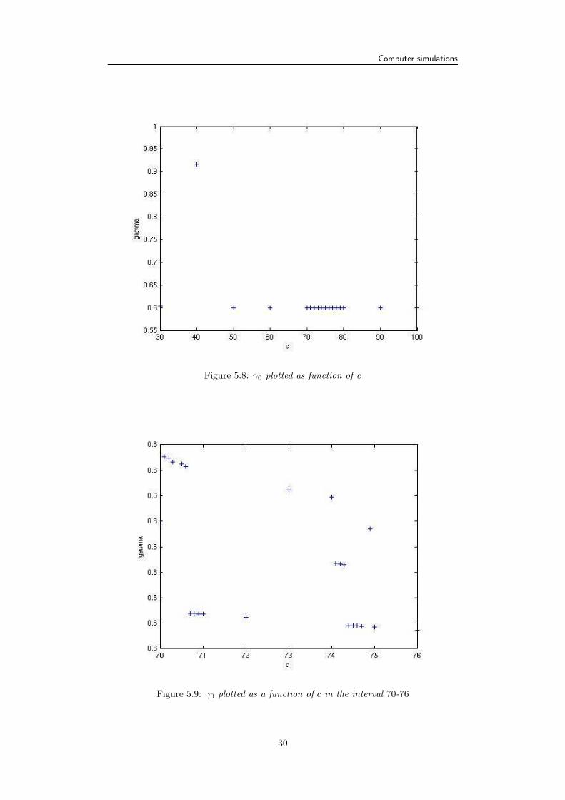
To find the minimum value for c, where the solution still obeys the condition for γ0.The program is ruined for different values of c, and the constant γ0 is determined.Then γ0 is plotted as a function of c, see figure 5.8.When the final value of γ0 exceeds its upper limit, the value of c becomes to small andthus it has to be increased. The interval where γ0 ecceed its upper value is between 70and 76. Therefore this area has to be investigated further. A plot of γ0 as a functionof c for the interval 70− 76 is shown in figure 5.9.From the figure it is noted that the value of γ0 is unstable from 70 to 76. Thereforethe constant c is changed to 76 to be sure of that the γ0 condition always is obeyed.To determine whether the change in the value of c has any influence on the opti-mization of the system or not, the simulation are performed for pressure differencesbetween ∆p = 0.5Pa and ∆p = 0.7Pa, because in this interval, the obtained solutionswere not the optimal solutions as they had to be. afterwards, the pressure is changedto determine the temperature for the systems.As noted from figure 5.10, the change in the c value does not have any influence onthe fact that the systems are not optimal at the pressure difference, they are opti-mized for. The pressure difference is very small and there is almost no change inthe structure of the design area. Therefore, the error might be caused because theprogram has found a global minimum for the structure at the pressure range. Theoptimization is solved numerically, and thus there is only a finite number of meshpoints in the simulation, and the solution can only be calculated as precise as theconvergence criterion determines.
5.0.9 Increase of the pressure difference
The pressure difference over the micro fluidic cooling systems is still to small to bemeasured because the pressure difference cannot exceed ∆p = 1.7Pa. Above thispressure, the channels start to terminate into the material, and thus the solutionsbecomes unphysical. To increase the pressure difference over the micro fluidic coolingsystem, a very long inlet is determined in FEMLab. The new structure is shown in
29
Computer simulations
Figure 5.8: γ0 plotted as function of c
Figure 5.9: γ0 plotted as a function of c in the interval 70-76
30

Computer simulations
Figure 5.10: Temperature plotted as a function of the pressure difference over theoptimized cooling system. The program is runnet with c = 76
figure 5.11.The wide of the inlet and outlet is changed to ∆p = 0.2cm, which makes it easierto draw the helical line i FEMLab. The simulations are runnet for different pressuredifferences over the system and it is discovered that the pressure difference cannotexceed ∆p = 2 Pa, because systems with a higher pressure difference has channelsthat terminates into the material, as illustrated on figure 5.12 .This structure is fabricated i a PMMA plate as described in section 6.1.
5.0.10 The final system
The pressure difference over the devices has to be even higher, and thus the systemsdescribed below could not be used for practical experiments. Therefore it was decidedto define the inlet and outlet as long helical line. This was not simulated in FEMLab,but defined with use of the laser program. It was possible ti calculate the pressuredifference over the micro fluidic cooling systems if the hydraulic resistant for the inletand outlet was determinated. The only part of the system that is simulated in FEM-Lab, is the design region. A the inlet and outlet, boundary conditions are defined inthe same way as earlier. The new structure is shown in figure 5.13. The temperatureof the water at the inlet is fixed to be T = 25C, corresponding to the temperatureof the water used in the experiments, that was the same as the temperature in thelab where the experiments were performed.The width of the inlet and the outlet is set to w = 0.5mm. The simulated wereperformed for pressure differences between ∆p = 0.5Pa and ∆p = 4Pa in steps of∆p = 0.5Pa. The obtained result is noted in figure 5.14.As noted from the figure, the systems optimized for higher pressure differences than∆p = 2.5Pa have channels that terminates into the material and thus these are un-physical.The pressure of the optimized systems is varied and the new temperatures are calcu-lated. The average temperature over the design region as a function of the pressure
31

Computer simulations
Figure 5.11: The geometry for the micro fluidic stucture with a long inlet, draw inFEMLab as a helical line.
Figure 5.12: The structure of a optimized micro fluidic cooling systems, optimized atdifferent pressures.
Ω1
Figure 5.13: Geometry of the final micro fluidic cooling systems.
32
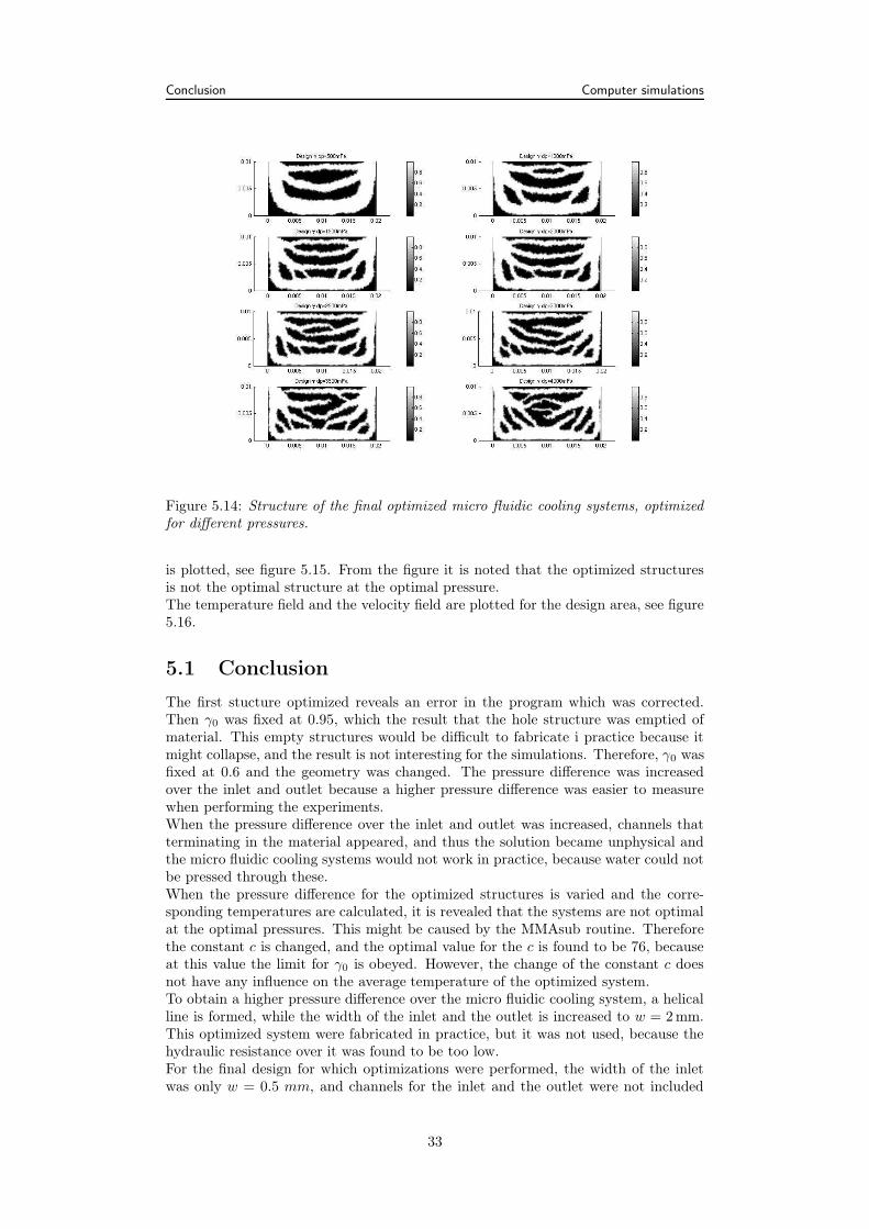
Conclusion Computer simulations
Figure 5.14: Structure of the final optimized micro fluidic cooling systems, optimizedfor different pressures.
is plotted, see figure 5.15. From the figure it is noted that the optimized structuresis not the optimal structure at the optimal pressure.The temperature field and the velocity field are plotted for the design area, see figure5.16.
5.1 Conclusion
The first stucture optimized reveals an error in the program which was corrected.Then γ0 was fixed at 0.95, which the result that the hole structure was emptied ofmaterial. This empty structures would be difficult to fabricate i practice because itmight collapse, and the result is not interesting for the simulations. Therefore, γ0 wasfixed at 0.6 and the geometry was changed. The pressure difference was increasedover the inlet and outlet because a higher pressure difference was easier to measurewhen performing the experiments.When the pressure difference over the inlet and outlet was increased, channels thatterminating in the material appeared, and thus the solution became unphysical andthe micro fluidic cooling systems would not work in practice, because water could notbe pressed through these.When the pressure difference for the optimized structures is varied and the corre-sponding temperatures are calculated, it is revealed that the systems are not optimalat the optimal pressures. This might be caused by the MMAsub routine. Thereforethe constant c is changed, and the optimal value for the c is found to be 76, becauseat this value the limit for γ0 is obeyed. However, the change of the constant c doesnot have any influence on the average temperature of the optimized system.To obtain a higher pressure difference over the micro fluidic cooling system, a helicalline is formed, while the width of the inlet and the outlet is increased to w = 2 mm.This optimized system were fabricated in practice, but it was not used, because thehydraulic resistance over it was found to be too low.For the final design for which optimizations were performed, the width of the inletwas only w = 0.5 mm, and channels for the inlet and the outlet were not included
33

Conclusion Computer simulations
Figure 5.15: The structure of the optimized micro fluidic cooling system, optimized atdifferent pressures.
in the simulations. The final structure was optimized for pressure differences up to∆p = 2.5 Pa, which was the highest pressure obtained for any of the optimized geome-try’s, before the channels started to terminate within the material. It would thereforebe reasonable to assume that if the inlet and the outlet were made even thinner itwould be possible to obtain geometries at higher pressure differences over the inletand outlet, before channels begin to terminate within the material.The two structures that was fabricated in practice, are chosen to be the systems opti-mized for ∆p = 0.5 pa and ∆p = 2.5 Pa, because the structures of these micro fluidiccooling systems did not have channels that terminated into the material.
34
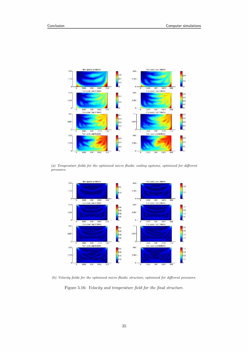
Conclusion Computer simulations
(a) Temperature fields for the optimized micro fluidic cooling systems, optimized for differentpressures.
(b) Velocity fields for the optimized micro fluidic structure, optimized for different pressures.
Figure 5.16: Velocity and temperature field for the final structure.
35

Chapter 6
Fabrication of micro fluidic
cooling systems
6.1 Fabrication of micro structures with a CO2 laser
For fabrication and further experiments performed with the topology optimized cool-ing systems, the structure of these were fabricated in poly methylmethacrylate poly-mer (PMMA) using a CO2 laser system. This fabrication method has many advanta-geous because it is very fast and simple and flexible for the purpose. The CO2 laserset-up is shown in figure 6.1
(a) The CO2 laser. (b) A piece of PMMA placed under the laserhead ready for fabrication of micro fluidicstructures.
Figure 6.1: CO2 laser set-up used for fabrication of the micro fluidic structures. Thelaser is connected to a computer.
The CO2 laser is an infrared laser representing a material removing fabrication method.It evaporates substrate material directly by applying heat with the laser beam. Theinfrared laser used is a carbon dioxide laser, which emits radiation at a wavelength ofλ = 10.6 µm.The material used for the micro fluidic structures is PMMA polymer, which has ahigh absorbance of about 0.92 in the infrared region. PMMA also combines a lowheat capacity with a low heat conductance. Therefore, any absorbed heat will resultin a rapidly rising temperature being able to melt some of the polymer.The laser system is controlled by a two dimensional computer CAD-program whichcontrols a mirror-equipped head deflecting and focussing the laser beam. Using thecomputer it is among other factors possible to set the power of the laser beam, thevelocity of it, the number of passes it makes over the same channel, the resolution
36

Fabrication of devices Fabrication of micro fluidic cooling systems
and the scan direction. The CAD-program can move the laser to any position withina square working field of 110 mm × 110 mm.However, the width, depth and profile of the fabricated channels are not only de-pending on the properties mentioned until now, but also, among other things, onthe optical properties of the laser system, the layout processing sequence, the natureof the laser ablation and thermodynamically properties of the polymer. The opticalproperties of the laser system determine the incident laser power, the spot size, thedepth of the field and the divergence of the laser beam, while the thermodynamicallyproperties of the polymer determine how it reacts to the beam.The evaporation mechanism of the polymer and the absorbance of it are temperaturedependent. The polymer is conducting heat away from the melting zone in an un-even manner, especially at the corners in the bottom of the channels; the conductingheat loss is always higher in these areas, which results in a decreased ablation here.Because of this the dimensions of the channels will change during the fabrication andtherefore can become very difficult to measure. From observed channel profiles mea-sures with an optical microscope they can be assumed to have a Gaussian profileThe conductive heat and capative heat loss terms causes a certain amount of heatthat is not available to evaporate from the PMMA and therefore disperses into theadjacent material. The size of the affected area depends on the relative amount ofthe heat loss terms and the time available for dispersing heat into the surroundingmaterial. It is observed that the channel width depends on the cutting sequence, andthe channel depth depends on the length of the channel. Therefore, if a channel iscut with more than one pass, the cooling time between the passes becomes relevant.The available cooling time depends on the channel length, which means that shorterchannels will be deeper at the same laser settings.Deflecting of the laser beam on surface produces the channels, when it hits the surfaceunder a changing angle while the beam moves. The consequence is that an absolutelysymmetric channel profile only can be produced if it is centred in the middle of thechannel direction below the head of the laser beam.The higher the velocity of the laser beam, the higher the relative heat loss into the sur-roundings of the structures will become, meaning that fine precise structures have tobe fabricated with lower velocities than straight channels. Observations have shownthat the channel depth in linearly proportional to the number of passes at a fixedvelocity. The channel size also depends on the spot size of the laser beam, which istime-dependent, since the resulting Gaussian profile does that a slow moving laserbeam results in broader channels than a fast moving beam.When PMMA is heated up, it remains in the solid glass state until it reaches glasstemperature at about 115C, while at higher temperatures it becomes easily rubberyand mouldable. If even more energy is added to the system, at temperatures be-tween 350C and 380C, thermal decomposition of PMMA begins, which does thatthe polymer chains spontaneous break during a process called propagation, leadingto development of monomers (MMA), which are volatile, but also carbon dioxide andother gasses evolve during the thermal decomposition of PMMA in the presence ofair.While cutting a channel the heat introduced into the polymer material also resultsin bulges or splashes running parallel to the channels because some of the polymermelts and is driven out of the channels. This may influence the quality of the bondingprocess, risking to clog the channels. Therefore, after fabricating of the micro fluidicstructures, it can be necessary to polish the cut plane to avoid artefacts from thecutting process that can distort the channel profiles. [3]
6.2 Fabrication of devices
For fabrication of the devices, it is very important that the structures of the fabricatedmicro fluidic cooling systems are in agreement with the topology-optimized structures
37

Fabrication of devices Fabrication of micro fluidic cooling systems
calculated with FEMLab and MatLab to get accurate measurements. Anyway, it isnever possible to avoid all sources of error, primary because of uncertainties whenusing the laser as described in section 6.1.The structures of the micro fluidic cooling systems are defined by the γ-field savedas a FEMLab file when running the optimization program. This file contains boththe structure of the inlet and outlet and the micro fluidic cooling system, becausethey were all included in the optimizations. The FEMLab-file describing the γ-fieldis converted into a Bitmap-file because the laser program, WinMark, can only readBitmap-files.Unfortunately, the resolution of the Bitmap-file is not good enough to prevent dentedpoints at the edges of the channels. Therefore an exact copy of the inlet and outletchannels was drawn using the program CorelDRAW. Using the program Corel Pho-toPaint, the black and white colours of the γ-field for the optimized micro fluidiccooling systems were inverted. All grey-scale colours were removed by setting thecontract of brightness to 100%, thereby trying to prevent mistakes at the edges. Atlast the two drawings were put together and exported as a PNG-file with a resolutionof 300 times 300 pixels, witch is the best advantage possible.After some tests it was decided by use of an electronic Vernier calliper gauge that thechannels has to be cut first horizontal and then vertical, so that the laser programhad to run in two sections. The best parameters giving channels that are 1 mm deepfor each of the two sections are,
Micro fluidic cooling system, inlet and outletMark passes 3Velocity 800 mm/sPower 20 %Resolution 1000
The rest of the parameters are as the default settings given by the WinMark laserprogram.To remove the device from the PMMA plate, after cutting the channels, a rectanglewas drawn around it and the device was cut using the laser. The size of the rectangleis so that the inlet and outlet go beyond it to prevent edges caused by the laser. Thechannels have to be in the middle of the devices, between the top and the bottom ofit. Therefore, because the channels are 1 mm deep, they were cut in a 2 mm thickPMMA plate, and for each device a lit was cut in a 1 mm thick PMMA plate, havingthe same size as the bottom with the channels cut.Afterwards the devices were bounded by pressing the top and bottom together byused of a clamp. Two metal blocks ensured that the force was even distributed overthe device, and the blocks were protected from the melting PMMA by use of a glasslayer during the bonding process. The devices were inserted in an oven and heated upto 109C for about 60 minutes. Devices in the oven during the bonding process areshown in figure 6.3. After the bonding process metal fittings were fastened at the inletand outlet with epoxy glue and so the devices were ready for further experiments.One of the final devices is shown in figure 6.2.
Unfortunately, afterwards it was concluded that the inlet and outlet channel weretoo broad and even not long enough to give a well-defined pressure difference thatcould be measured with use of the pressure sensors, and so experiments were neverperformed on these cooling systems. Therefore new devices had to be fabricated.
6.2.1 Fabrication of new devices
The width of the inlet and outlet of the devices had to be smaller, and the size of it wasestablished to be 0.5 mm. Thus new micro fluidic cooling system had to be optimized
38
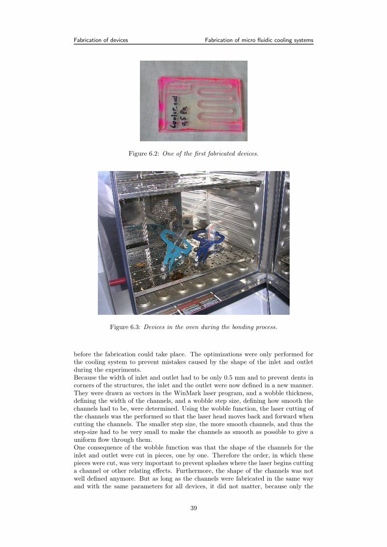
Fabrication of devices Fabrication of micro fluidic cooling systems
Figure 6.2: One of the first fabricated devices.
Figure 6.3: Devices in the oven during the bonding process.
before the fabrication could take place. The optimizations were only performed forthe cooling system to prevent mistakes caused by the shape of the inlet and outletduring the experiments.Because the width of inlet and outlet had to be only 0.5 mm and to prevent dents incorners of the structures, the inlet and the outlet were now defined in a new manner.They were drawn as vectors in the WinMark laser program, and a wobble thickness,defining the width of the channels, and a wobble step size, defining how smooth thechannels had to be, were determined. Using the wobble function, the laser cutting ofthe channels was the performed so that the laser head moves back and forward whencutting the channels. The smaller step size, the more smooth channels, and thus thestep-size had to be very small to make the channels as smooth as possible to give auniform flow through them.One consequence of the wobble function was that the shape of the channels for theinlet and outlet were cut in pieces, one by one. Therefore the order, in which thesepieces were cut, was very important to prevent splashes where the laser begins cuttinga channel or other relating effects. Furthermore, the shape of the channels was notwell defined anymore. But as long as the channels were fabricated in the same wayand with the same parameters for all devices, it did not matter, because only the
39

Fabrication of devices Fabrication of micro fluidic cooling systems
resistance over the inlet and outlet was important, the reason being that these werenot included in the FEMLab optimizations. For determination of the resistance ofthe inlet and outlet channel, a device was fabricate without any micro fluidic coolingsystem, but with the same length of the channels as for the devices containing themicro fluidic cooling systems. This device and the one of the devices including a microfluidic cooling system are shown in figure 6.4. The parameters used when cutting the
(a) Device fabricated for measurement of theresistance of the inlet and outlet.
(b) Device with a micro fluidic cooling sys-tem including inlet and outlet. The pressuredifference over the micro fluidic cooling sys-tem has to be 2.5 Pa. .
Figure 6.4: The inlet and outlet for the micro fluidic cooling systems. These deviceswere unfortunately too big to be bounded well enough.
micro fluidic cooling system with the laser were the same as for the first fabricatedsystems. At the inlet and outlet at the boundaries of the devices the channels weremade a little broader and deeper making it possible to glue a metal inlet and outletto the devices. The parameters used when cutting the inlet and outlet are shown inthe table below. The cooling systems were still cut in a 2 mm PMMA plate and thelids were still cut in a 1 mm PMMA plate.
Inlet and outlet Inlet and outlet at boundariesMark passes 2 2Velocity 800 mm/s 800 mm/sPower 30 % 45 %Resolution 300 300Wobble On OnWobble thickness 0.50 mm 1.30 mmWobble step size 0.05 mm 0.05 mm
The size of the new devices was about 6 cm × 6 cm and so new metal blocks werefabricated for the bonding process to distribute the force equally over the devices.Unfortunately it did not succeed to make more than a few good devices becausealmost all of them were not bonded well enough, and thus they were leaking water.
6.2.2 Fabrication of the final devices
A solution to the bonding problem might be to make the devices smaller for a betterdistribution of the power during the bonding process. Therefore a new inlet andoutlet were defined in the WinMark laser program in the same manner as for theprevious devices, but with less distance between the inlet and outlet channels. Thenew devices were cut using the same laser parameters as previous, and both deviceswith and without micro fluidic cooling systems were fabricated. Furthermore a devicecontaining a simple test structure, a one 1 mm deep, broad, twisted channel, insteadof a cooling system was defined as a vector in WinMark an fabricated for examination
40
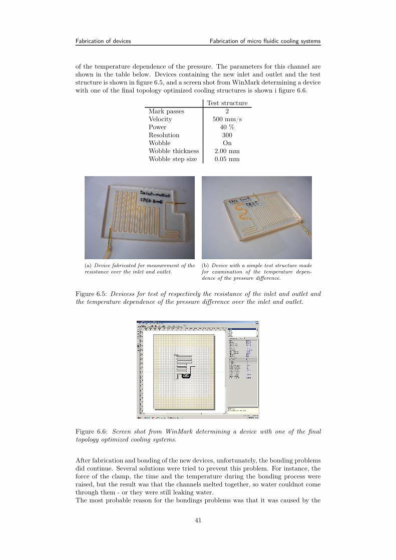
Fabrication of devices Fabrication of micro fluidic cooling systems
of the temperature dependence of the pressure. The parameters for this channel areshown in the table below. Devices containing the new inlet and outlet and the teststructure is shown in figure 6.5, and a screen shot from WinMark determining a devicewith one of the final topology optimized cooling structures is shown i figure 6.6.
Test structureMark passes 2Velocity 500 mm/sPower 40 %Resolution 300Wobble OnWobble thickness 2.00 mmWobble step size 0.05 mm
(a) Device fabricated for measurement of theresistance over the inlet and outlet.
(b) Device with a simple test structure madefor examination of the temperature depen-dence of the pressure difference.
Figure 6.5: Devicess for test of respectively the resistance of the inlet and outlet andthe temperature dependence of the pressure difference over the inlet and outlet.
Figure 6.6: Screen shot from WinMark determining a device with one of the finaltopology optimized cooling systems.
After fabrication and bonding of the new devices, unfortunately, the bonding problemsdid continue. Several solutions were tried to prevent this problem. For instance, theforce of the clamp, the time and the temperature during the bonding process wereraised, but the result was that the channels melted together, so water couldnot comethrough them - or they were still leaking water.The most probable reason for the bondings problems was that it was caused by the
41

Fabrication of devices Fabrication of micro fluidic cooling systems
PMMA, because the two PMMA plates at respectively the top and bottom of thedevices were made of two different kinds of PMMA, or the surface of top plate wascoated with something that did not bind very well to the bottom plate while thesewere bonded together.It was tried to remove the possible surface coating with ethanol, but this was not agod idea, because it resulted in cracks within the PMMA caused by stress within it.Thus the solution to this problem was to use the same kind of PMMA for the top andthe bottom, even though it had the consequence that the micro fluidic structure wouldnot be in the middle of the devices. Therefore, now 1.5 mm thick PMMA plates wereused for the top, and the micro fluidic cooling systems, inlet and outlet were cut in2 mm thick PMMA plates for the bottom. Then it was succeeded to fabricate somedevices that could be used for experiments.
6.2.3 Conclusion
Fabrication of devices with micro fluidic cooling systems is not always an easy processbecause a lot of factors enters in the fabrication process.It is not easy to find the most optimale bonding force, time and temperature, wherebonding always will succeed - if there are any. And uncertainties during the lasercutting will always cause some uncertainties that cannot be prevented. Therefore itmight be difficult to reproduce devices, but it was tried as good as possible.It is not optimal that the cooling systems fabricated at last were not in the middleof the devices because of the thickness of the PMMA plates, which was 1.5 mm and2 mm, because it by no means was possible to used the 1 mm PMMA plates because itwould not bound to the other PMMA plates. A solution to this problem might be toremove 1 mm of the 2 mm PMMA plates and then use it. But this was not found tobe necessary because the uncertainties for further measurements of the temperaturewould not have been prevented anyway.When bonding is performed on PMMA plates in the clean room at DANCHIP, DTU,the plates are first heated up to 80C for some amount of time. During his process allstress will disappear from the PMMA, and it ten becomes possible to clean the PMMAplates and thereby remove all dirt from the surfaces using ethanol instead of water.Furthermore the plates would have become totally flat, preventing it from bendingbecause of the heat arising during the cutting of channels with the laser. Thus if thisprocess were performed to the devices in this project, the bonding process might havebeen easier.Another idea might have been to try to make the size of the devices even smaller,thereby a more equal distribution of the force during the bonding process wouldhave been possible. The size of the devices was minimized when fabricating the lastdevices, but because, at last, some of these were successfully bonded, it was not foundnecessary to make the devices even smaller.
42

Chapter 7
Experimental set-up
To heat up the micro fluidic cooling systems while running the experiments, a heat-ing element is placed under the structure of it. Cobber plates on the top of coolingsystems and below it, between the heating element and the cooling system, are placedfor a uniform distribution of the heat. The size of the micro fluidic cooling systemsis 1 cm × 2 cm, and so the size of the heating element and the cobber sheets are thesame. The size of the whole device is, of cause, bigger than the micro fluidic coolingsystem itself, but heat only have to be applied to the cooling system, not on the inletand outlet channels.The "sandwich" consisting of the micro fluidic cooling system, the heating elementand the cobber plates is placed on a holder and fixed by use of a clips. Betweenthe layers "cooling" plasma is applied to glue the parts together and to give a betterdistribution of the heat through these. The "sandwich" is shown in figure 7.1.
Inlet
Plastic sheets
microfluidic structure
Topology optimized
Heating element
Cobber sheet
Cobber sheet
Outletpressure sensorsConnection with
Measurement of temperature
Measurement of temperature
Figure 7.1: "Sandwich" consisting of a micro fluidic cooling systems, a heating elementand cobber sheets.
To measure the temperature of the cobber sheets, small holes are drilled in whichtemperature sensors or so-called thermistors are mounted.A plastic bag containing small, isolating styrene balls covers the "sandwich" to pre-vent heat flow from it. Thereby the heat of the cobber plate on the top of the coolingsystem will heat up faster and so the temperature of it will become higher than with-
43

Measurements of pressure and temperature Experimental set-up
out the isolating.Water is sent through a tube connection to the system with a constant velocity or flowrate by use of a glass squirt mounted on a squirt pump. When starting performingexperiments a plastic squirt was used, but it was determined that it was not wellsuited for the purpose, because plastic is very soft compared to glass, resulting incomparatively long relaxation times for the pressure over the system. The tube, thewater is send through, is made of Teflon, that is a relatively hard material, to preventextensions of it during the experiments. However, connections between for instancethe tube and the device are made of small pieces of silicone tube. When the waterhas been send all the way through the system it drips out into a bowl placed at theend of the tube.Just before and after the device the tubes are connected to pressure sensors for mea-surement of the pressure difference over the device. When measuring the pressureit is very important that the height of pressure sensor is the same. Therefore theconnections to the sensors are taped to the same metal box.The pressure tensor connected to the system at the outlet of the devices will measurethe atmospheric pressure, or almost atmospheric pressure, because no system afterthe outlet can cause a change in the pressure. Anyway, it is necessary yo have apressure sensor at the outlet, because there will be small variation in the pressure,and these have an important influence on the experiments, because small pressured-ifferences have to be measured.The pressure sensors and the temperature sensors are connected to an electronicboard, which gets a constant power from a power supply. The heating element isconnected to another power supply. Furthermore the electronic board is connectedto a computer with LabView installed. The LabView program measures the voltageoutput of the pressure sensors and the temperature sensor, which afterward have tobe translated into respectively pressure and temperature by use of data sheets for thecomponents.A schematic drawing of the set-up is shown in figure 7.2, and a picture of it is shownin figure 7.3.
7.1 Measurements of pressure and temperature
7.1.1 The pressure sensors
Two electrical pressure sensors are used to measure the pressure over the micro fluidiccooling systems, at respectively the inlet and the outlet of the system.A pressure sensor is a little electronic device that is split up into two parts separatedby a thin electrical conducting membrane. The pressure sensors are connected to thecooling system with a T-fitting and a tube just before the inlet and just after theoutlet.The tube has to be completely filled with water, because otherwise the measurementof the pressure will not be exact, because air in the tube will be compressed wheninfluenced by a pressure.When water is sent through the cooling system, the membrane is influenced and sothe electrical resistance of the pressure tensor is changed. Each pressure sensor willthen give an output voltage, which can be converted into a pressure. [7]
7.1.2 Measurement of pressure
The output of the pressure sensors measured with the LabView program is a voltageand not directly a pressure. Therefore, to determine the pressure, it is necessary to
44

Measurements of pressure and temperature Experimental set-up
Power supplyPower supply
Computer with LabView
Squirt pump
computerConnection to
Temperature sensorsPressure sensors
Bowl for water outlet
Electronic board
Cobber sheets
Micro fluidic cooling system
Figure 7.2: Schematic drawing of the experimental set-up. A plastics bag containingsmall, isolating styrene balls covers the "sandwich", but this it not shown on thedrawing.
Figure 7.3: Set-up for the experiments. The plastics bag containing small, isolatingstyrene balls covering the "sandwich" is not shown on the picture.
45
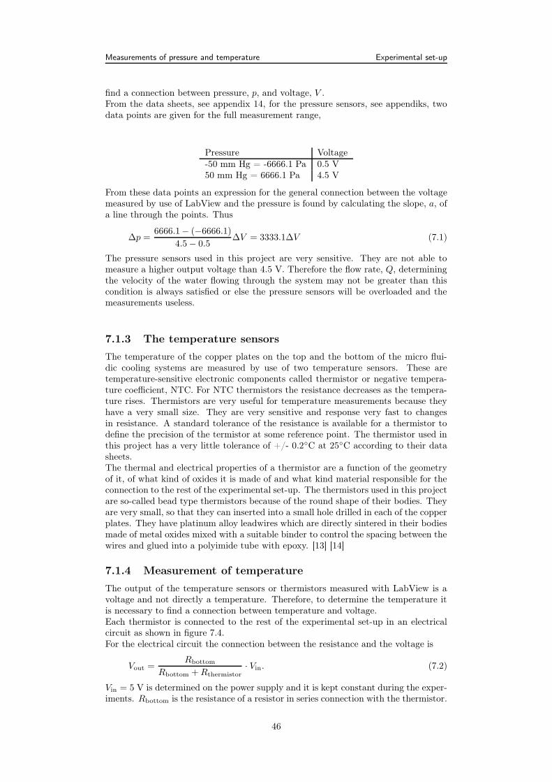
Measurements of pressure and temperature Experimental set-up
find a connection between pressure, p, and voltage, V .From the data sheets, see appendix 14, for the pressure sensors, see appendiks, twodata points are given for the full measurement range,
Pressure Voltage-50 mm Hg = -6666.1 Pa 0.5 V50 mm Hg = 6666.1 Pa 4.5 V
From these data points an expression for the general connection between the voltagemeasured by use of LabView and the pressure is found by calculating the slope, a, ofa line through the points. Thus
∆p =6666.1− (−6666.1)
4.5 − 0.5∆V = 3333.1∆V (7.1)
The pressure sensors used in this project are very sensitive. They are not able tomeasure a higher output voltage than 4.5 V. Therefore the flow rate, Q, determiningthe velocity of the water flowing through the system may not be greater than thiscondition is always satisfied or else the pressure sensors will be overloaded and themeasurements useless.
7.1.3 The temperature sensors
The temperature of the copper plates on the top and the bottom of the micro flui-dic cooling systems are measured by use of two temperature sensors. These aretemperature-sensitive electronic components called thermistor or negative tempera-ture coefficient, NTC. For NTC thermistors the resistance decreases as the tempera-ture rises. Thermistors are very useful for temperature measurements because theyhave a very small size. They are very sensitive and response very fast to changesin resistance. A standard tolerance of the resistance is available for a thermistor todefine the precision of the termistor at some reference point. The thermistor used inthis project has a very little tolerance of +/- 0.2C at 25C according to their datasheets.The thermal and electrical properties of a thermistor are a function of the geometryof it, of what kind of oxides it is made of and what kind material responsible for theconnection to the rest of the experimental set-up. The thermistors used in this projectare so-called bead type thermistors because of the round shape of their bodies. Theyare very small, so that they can inserted into a small hole drilled in each of the copperplates. They have platinum alloy leadwires which are directly sintered in their bodiesmade of metal oxides mixed with a suitable binder to control the spacing between thewires and glued into a polyimide tube with epoxy. [13] [14]
7.1.4 Measurement of temperature
The output of the temperature sensors or thermistors measured with LabView is avoltage and not directly a temperature. Therefore, to determine the temperature itis necessary to find a connection between temperature and voltage.Each thermistor is connected to the rest of the experimental set-up in an electricalcircuit as shown in figure 7.4.For the electrical circuit the connection between the resistance and the voltage is
Vout =Rbottom
Rbottom + Rthermistor· Vin. (7.2)
Vin = 5 V is determined on the power supply and it is kept constant during the exper-iments. Rbottom is the resistance of a resistor in series connection with the thermistor.
46

Measurements of pressure and temperature Experimental set-up
Vout
Vin
Rthermistor
Rbottom
Figure 7.4: Schematic drawing of the set-up with each of the thermistors.
The resistance of this is measured by use of an ohmmeter to be Rbottom = 2491Ω.From the data sheets, see appendix 14, for the thermistors, see appendiks, the connec-tion between temperature T , and measured resistance, Rthermistor, is given for someparticular values of the resistance. By inserting this data points in the expression 7.2,it is possible to determine a connection between the output voltage, Vout, and thetemperature, T , for each value of Rthermistor.Plotting and curve through the determined points and calculating a function for thebest line through them gives an expression for he general connection between theoutput voltage measured with LabView and the temperature,
T = 23.234Vout + 2.6075 (7.3)
The expression for connection between output voltage and temperature is shown infigure 7.5.
Figure 7.5: Connection between output voltage and temperature.
47
Chapter 8
Experiments
8.1 Relaxation time of the system
8.1.1 Purpose
When performing the first experiments in this project, water was sent through thesystem by use of the syringe pump with a plastic syringe mounted. Unfortunately itwas observed, that it took a disproportionate amount of time for the system to relaxand the pressure to become the same for the two pressure sensors after the pump wasstopped.The reason for this phenomenon is that plastic is a relatively soft material The resis-tance of it is very high, and it will be pressed together and react as a spring whenexposed to a force of for instance the syringe pump.If the relaxation time for the system is very long, it will be difficult to perform experi-ments, and it will be necessary to wait a relatively long time between measurements.Furthermore, a long relaxation time will result in unwanted uncertainties.Therefore the plastic syringe was replaced with a glass syringe. Glass is a relativelyhard material, but it will still take a while for the system to relax. Therefore, toobtain welther the relaxation time has a major influence on the experiments or not,this has to be examined.
8.1.2 Method of approach
Instead of a device containing a micro fluidic cooling system, a Teflon tube is mountedon the system between the two pressure sensors measuring the pressure over the inletand the outlet, respectively. The length of the tube is L = 24.2 cm, and the radius ofit is a = 0.4 mm.A glass syringe is filled with water and mounted on the syringe pump, and the pumpis started with a flow rate being Q = 3 ml/min = 5.01·10−8 m3/s. When the pressureat the inlet seems to be constant, the pump is stopped, and thus the system will relax.The pressure measure at the inlet and the outlet is continuous written to a file andsaed by used of LabView.
8.1.3 Data processing
The measurement points gives a voltage which has to be converted into a pressure.This is done as explained in section 7.1.2. 50 measurement points are obtained eachsecond. Therefore it takes 1/50 second between two measurement points and thus atime scale is defined.Now, the pressure measured at respectively the inlet and the outlet of the is plottedas a function of the time as shown in figure 8.1.
48
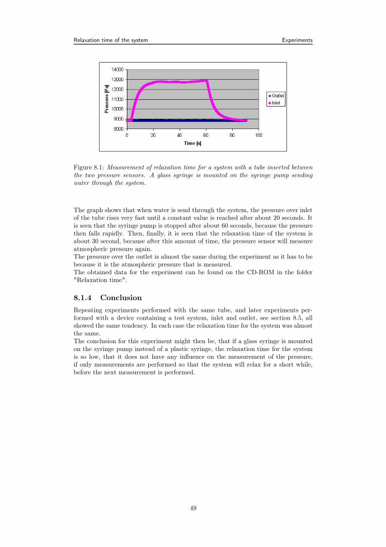
Relaxation time of the system Experiments
Figure 8.1: Measurement of relaxation time for a system with a tube inserted betweenthe two pressure sensors. A glass syringe is mounted on the syringe pump sendingwater through the system.
The graph shows that when water is send through the system, the pressure over inletof the tube rises very fast until a constant value is reached after about 20 seconds. Itis seen that the syringe pump is stopped after about 60 seconds, because the pressurethen falls rapidly. Then, finally, it is seen that the relaxation time of the system isabout 30 second, because after this amount of time, the pressure sensor will measureatmospheric pressure again.The pressure over the outlet is almost the same during the experiment as it has to bebecause it is the atmospheric pressure that is measured.The obtained data for the experiment can be found on the CD-ROM in the folder"Relaxation time".
8.1.4 Conclusion
Repeating experiments performed with the same tube, and later experiments per-formed with a device containing a test system, inlet and outlet, see section 8.5, allshowed the same tendency. In each case the relaxation time for the system was almostthe same.The conclusion for this experiment might then be, that if a glass syringe is mountedon the syringe pump instead of a plastic syringe, the relaxation time for the systemis so low, that it does not have any influence on the measurement of the pressure,if only measurements are performed so that the system will relax for a short while,before the next measurement is performed.
49

Heat conduction through a PMMA plate Experiments
8.2 Heat conduction through a PMMA plate
8.2.1 Purpose
At one stage it was tried to heat up a device containing a micro fluidic cooling systemwith stationary water to obtain whether the two copper plates in a "sandwich" con-taining the micro fluidic cooling system, the heating element and the copper plateswould obtain the same temperature or not.The power of the heating element were turned on, so that the temperature of thebottom copper plate was about 50 C, and the measurements were started. Unfor-tunately, after the system had been left to it own for almost a day, the temperatureof the upper copper plate was only raised about 5C compared to room temperature,which was the consequence of, that the heat would be conducted away from the sys-tem to the surrounding air, although air actually is a relatively good isolator becausethe thermal conductivity of it is very low.Therefore it was concluded that it was necessary to have some kind of isolating tocover the system. Thus a plastic bag were filled with small styrene balls and placedon the system so that the isolating layer were about 10 cm.To estimate the effect of the isolating layer in a more experimental way than previous,measurements were now performed with a piece of PMMA between the two copperplates, both for an isolated and for an unisolated system. Furthermore, the results ofthe experiments were compared to a FEMLab simulation of the heat flow through a"sandwich" structure containing a PMMA plate between two copper plates.
8.2.2 Method of approach
A piece of a PMMA plate was placed between the two copper plates, above the heat-ing elements. The size of the PMMA plate was 4 cm × 4 cm, and the thickness ofit was 2 mm. For the first measurement, the system was not isolated, while for thesecond measurement a plastic bag containing small styrene balls was used to isolatethe system from the surroundings, so that the thickness of the isolating layer wasabout 10 cm.The power was turned on the heating element, and it it was heated up. The temper-ature of the two copper plates was measured for about an hour. One measurementpoint was obtained each second. The power to the heating element was the same forboth experiments.The obtained data for the experiments can be found on the CD-ROM in the folder"PMMA".
8.2.2.1 FEMLab simulations
Afterwards, simulations of the heat conduction was performed by use of FEMLab us-ing a Transient Analyze under the "Heat Transfer by Conduction" application mode.The simulations were performed for a system containing a PMMA plate placed be-tween two copper plates, having the same dimensions as in the experiment, fir wichthe surface of the bottom plate was heated up. The simulations were performed forboth an isolated system and for an unisolated system surrounded by 10 cm air. Inboth cases the heat conduction was obtained at different times to obtain how thetemperature through system would behave as function of time and thickness of the"sandwich". The simulation time was stated to be an hour.The physical constants for PMMA, copper and air used in the simulation are,
50

Heat conduction through a PMMA plate Experiments
PMMA Copper AirThermal conductivity, k 0.21 W/(m·K) 400 W/(m·K) 0.0271 W/(m·K)Heat capacity, c 1190 J/(kg·K) 8700 J/(kg·K) 1005 J/(kg·K)Density, ρ 1470 kg/m3 385 kg/m3 1.127 kg/m3
The surface temperature of the bottom copper plate was defined to be 35C, becauseFEMLab defines the zero-point reference temperature to be 0C. Thus if the the roomtemperature is assumed to be 25C, the temperature of the copper plate becomes60C − 25C = 35C, which is assumed to be a reasonable value compared to thetemperature, that will be measured for an sisolated system below.
8.2.3 Data processing
The output voltage from the temperature sensor are converted into a temparatureas explaned in section 7.1.4. The temperature sensors connected to the two copperplates measure a voltage and not directly a temperature. Therefore the measuredvoltage are converted into a temperaturse as described in section 7.1.4.For both the isolated and the unisolated system, the temperature of the upper and thebottom copper plate is plotted as function of the time, at which the system is heatedup, see figure 8.2(a) and figure 8.3(a), respectively. Furthermore, the temperaturedifference between the two copper plates, Ttop −Tbottom, was determined and plottedas function of the time, see figure 8.2(b) and figure 8.3(b), respectivelyFrom figure 8.2(a) it is noted, that for the unisolated system the temperature of the
(a) Temperature of respectively the top andthe bottom copper plate as function of time.
(b) Temperature difference as function oftime.
Figure 8.2: Temperature as function of time for the uinsolated system.
(a) Temperature of respectively the top andthe bottom copper plate as function of time.
(b) Temperature difference as function oftime.
Figure 8.3: Temperature as function of time for the system isolated by a layer ofstyrene balls inside a plastic bag.
upper copper plate was almost constant during the experiment. The temperature ofthe bottom copper plate rises very slowly and it will take a long time before the tem-perature of it reachess a constant value. After performing the experiment for more
51

Heat conduction through a PMMA plate Experiments
than an hour, the temperature of the bottom copper plate was only about 32C whichis only about 2C more than the temperature of the bottom copper plate.From figure 8.3(a) it is noted, that the temperature of both the bottom and the up-per copper plate rises exponential during the whole experiment. After performing themeasurements for an hour, the temperature of the bottom copper plate was about48C, while the temperature of the upper copper plate was about 60C. The measuredtemperatures of the two copper plates therefore were much higher compared to theuisolated system.The plot of the temperature difference for the top and the bottom copper plate forthe unisolated system, see figure 8.2(b), shows that the temperature difference in-creases and becomes constants, as the system is heated up. However, after a while itreached a constant, but very low value being about 2C. The plot of the temperaturedifference for the isolated system, on the other hand, see figure 8.3(b), shows thatthe temperature difference indicate a tendency of being an exponential decreasingcurve, because the temperature of both the top and the bottom copper plate increaseexponentially.
8.2.3.1 Data processing of FEMLab simulations
For the FEMLab simulations, the profile of the heat flow through the "sandwich"structure for the isolated system is shown in figure 8.4. From the figure it is notedthat the temperature of the two copper plates is almost the same after a hour. Thisis not in accordance withs the results obtained for the experimal set-up, where thetemperature difference between the two cobber plates is significant and constant aftera while. Futhermore it is noted that the temperature is lowest at the edges of thePMMA plate, because it takes a while before the heat is conducted into these areas,while these are not directly heated.
Figure 8.4: Profile of the heat flow through the "sandwich" structure at different timessimulated by use of FEMLab.
Profiles of the heat flow through the middle of the "sandwich" structures, shownby the red line in figure 8.4, plotted as function of the thickness for the unisolated
52

Heat conduction through a PMMA plate Experiments
system and for the isolated system, see figure 8.5(a) and figure 8.5(b), respectivily.The heat profiles are shown for times between 100 s and 3600 s, with 100 s betweeneach calculated profile.
(a) Temperature as function of thickness foran unisolated system.
(b) Temperature as function of time for anisolated system.
Figure 8.5: Temperature as function of thickness for a "sandwich" structure contain-ing a PMMA plate between two copper plates, where the bottom plate is heated up.The heat conduction is shown at various times.
From the figures it is notes that there is a difference in the conduction for the isolatedand the unisolated system. At short times, it has an effect that the system is isolated,but as the time tends to an hour or more, the heat conduction through the isolatedand unisolated system is almost the same. The heat conduction through the copperplates as function of the time is noted to be an almost straight line, because thethermal conductivity of copper is very high compared to the thermal conductivityof PMMA, and thus the line showing the heat conductance as function of time forPMMA is a decreasing line.
8.2.4 Conclusion
The results of the experiments obtained for an unisolated system and for a isolatedsystem is very different. For the unisolated system almost all heat is conducted intothe sorroundings, resulting in a very small temperature difference between the twocopper plates after an hour. When the system is not isolated, the heating elementwill in principle have to heat up the whole room, until the temperature everywhere isthe same.For the isolated system, on the ohter hand, the temperature difference shows a ten-dence of forming an exponential decreasing curve, tending to a constant value after ashort while. The isolating styrene balls therefore has a major effect on the amount ofheat conducted away from the two cobber plates, and the temperature of the wholesystem raises more rapidly when it is isolated.The temperature difference is obtained because it is not possible to prevent loss ofenergy into the sorrundings. However, for the micro fluidic cooling systems it is notthe absolute temperature that is interesting, but the temperature difference of the twocobber plates. Thus, it is the temperature difference obtained for different coolingsystems, that has to be obtanied, when experiments are performed with water flowingthrough these with a well-defined pressure over the inlet and outlet.Finally, the conclusion of the experiments is, that when performing experiments onthe micro fluidic cooling system, these have to be isolated.The two FEMLab simluations yield almost the same result for the isolated and forthe unisolated system, and they are very different from the obtained experimentalresults. The reason for this might be that the unisolated system simulated by FEM-Lab is only sorrounded by 10 cm air, and air is a comparatively good isolator. The
53

Heat conduction through a PMMA plate Experiments
isolated system simulated with FEMLab is totally isolated, while this is not the casefor the system in the experimental set-up. Thus a better maching of the simulationsand the experiments might be obtained, if the system in the experimental set-up wasbetter isolated. However, it is not possible to avoid thermal heat conduction into thesorrounding totally.An other reason why the results obtained results for the simulations and the experi-ment differ, is that only conduction is included within the FEMLab simulations, eventhougt convection might also be represented, but the influence on the results causedby convection is very difficult to predict, because it is caused by movements withinthe system. Thus, convection is not included in the FEMLab simulations.
54
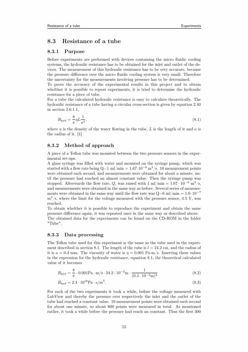
Resistance of a tube Experiments
8.3 Resistance of a tube
8.3.1 Purpose
Before experiments are performed with devices containing the micro fluidic coolingsystems, the hydraulic resistance has to be obtained for the inlet and outlet of the de-vices. The measurement of this hydraulic resistance has to be very accurate, becausethe pressure difference over the micro fluidic cooling system is very small. Thereforethe uncertainty for the measurements involving pressure has to be determined.To prove the accuracy of the experimental results in this project and to obtainwhelther it is possible to repeat experiments, it is tried to determine the hydraulicresistance for a piece of tube.For a tube the calculated hydraulic resistance is easy to calculate theoretically. Thehydraulic resistance of a tube having a circular cross-section is given by equation 2.40in section 2.6.1.1,
Rhyd =8
πηL
1
a4, (8.1)
where η is the density of the water flowing in the tube, L is the length of it and a isthe radius of it. [1]
8.3.2 Method of approach
A piece of a Teflon tube was mounted between the two pressure sensors in the exper-imental set-ups.A glass syringe was filled with water and mounted on the syringe pump, which wasstarted with a flow rate being Q=1 ml/min = 1.67·10−8 m3/s. 10 measurement pointswere obtained each second, and measurements were obtained for about a minute, un-til the pressure had reached an almost constant value. Then the syringe pump wasstopped. Afterwards the flow rate, Q, was raised with 1 ml/min = 1.67 · 10−8 m3/s,and measurements were obtained in the same way as before. Several series of measure-ments were obtained in the same way until the flow rate was Q=6 ml/min = 1.0 ·10−7
m3/s, where the limit for the voltage measured with the pressure sensor, 4.5 V, wasreached.To obtain whelther it is possible to reproduce the experiment and obtain the samepressure difference again, it was repeated once in the same way as described above.The obtained data for the experiments can be found on the CD-ROM in the folder"Tube".
8.3.3 Data processing
The Teflon tube used for this experiment is the same as the tube used in the experi-ment described in section 8.1. The length of the tube is l = 24.2 cm, and the radius ofit is a = 0.4 mm. The viscosity of water is η = 0.001 Pa·m/s. Inserting these valuesin the expression for the hydraulic resistance, equation 8.1, the theoretical calculatedvalue of it becomes
Rhyd =8
π· 0.001Pa · m/s · 24.2 · 10−2m · 1
(0.4 · 10−3m)4(8.2)
Rhyd = 2.4 · 1010Pa · s/m3. (8.3)
For each of the two experiments it took a while, before the voltage measured withLabView and thereby the pressure over respectively the inlet and the outlet of thetube had reached a constant value. 10 measurement points were obtained each secondfor about one minute, so about 600 points were measured in total. As mentionedeatlier, it took a while before the pressure had reach an constant. Thus the first 300
55
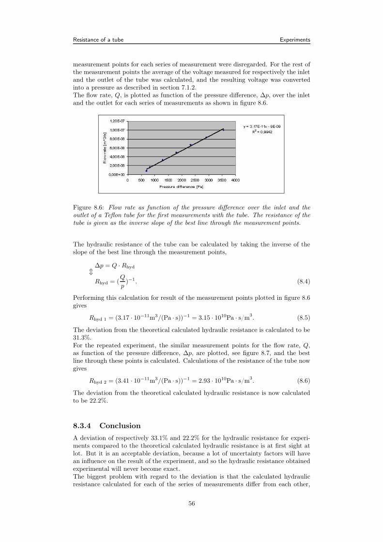
Resistance of a tube Experiments
measurement points for each series of measurement were disregarded. For the rest ofthe measurement points the average of the voltage measured for respectively the inletand the outlet of the tube was calculated, and the resulting voltage was convertedinto a pressure as described in section 7.1.2.The flow rate, Q, is plotted as function of the pressure difference, ∆p, over the inletand the outlet for each series of measurements as shown in figure 8.6.
Figure 8.6: Flow rate as function of the pressure difference over the inlet and theoutlet of a Teflon tube for the first measurements with the tube. The resistance of thetube is given as the inverse slope of the best line through the measurement points.
The hydraulic resistance of the tube can be calculated by taking the inverse of theslope of the best line through the measurement points,
∆p = Q · Rhydm
Rhyd = (Q
p)−1. (8.4)
Performing this calculation for result of the measurement points plotted in figure 8.6gives
Rhyd 1 = (3.17 · 10−11m3/(Pa · s))−1 = 3.15 · 1010Pa · s/m3. (8.5)
The deviation from the theoretical calculated hydraulic resistance is calculated to be31.3%.For the repeated experiment, the similar measurement points for the flow rate, Q,as function of the pressure difference, ∆p, are plotted, see figure 8.7, and the bestline through these points is calculated. Calculations of the resistance of the tube nowgives
Rhyd 2 = (3.41 · 10−11m3/(Pa · s))−1 = 2.93 · 1010Pa · s/m3. (8.6)
The deviation from the theoretical calculated hydraulic resistance is now calculatedto be 22.2%.
8.3.4 Conclusion
A deviation of respectively 33.1% and 22.2% for the hydraulic resistance for experi-ments compared to the theoretical calculated hydraulic resistance is at first sight atlot. But it is an acceptable deviation, because a lot of uncertainty factors will havean influence on the result of the experiment, and so the hydraulic resistance obtainedexperimental will never become exact.The biggest problem with regard to the deviation is that the calculated hydraulicresistance calculated for each of the series of measurements differ from each other,
56
Resistance of a tube Experiments
Figure 8.7: Flow rate as function of the pressure difference over the inlet and theoutlet of a Teflon tube for the sencond measurements with the tube. The resistance ofthe tube is given as the inverse slope of the best line through the measurement points.
although these experiments were obtained in the same way and without any changesin the set-up. Therefore, a conclusion might be that is not possible, or it is verydifficult, to repeat the experiments and get the same results.The deviation in the experimental result from the theoretical calculation can be causedby many factors. The greatest problem might be the connection of the tube to therest of the system, at the inlet and outlet of it, which is performed with a short pieceof silicon tube. The dimensions of this tube are not included in the calculations andmight, of cause, result in an error. Moreover, these small pieces of tube are madeof silicone which is a fairly soft material, that perhaps might be able to a bit whilewater is send through them causing their radius to rise. This does also explain whythe pressure calcaluted for the experiments becomes lower than the theoretical calcu-lated pressure. The tube at which the experiments is performed, is made of Teflon,which is a fairly hard material, and thus extension of it during the experiments isnot estimated to be a problem. But for the tube there will be a some unsertaintyfor its radius stated by the producer. Therefore there will not only be unsertaintiesfor hydraulic resistanse obtained from the experiments, but also for the theoreticalhydraulic resistance calculated for the tube.Anyway, for the following experiments, there will not be time to repeat these a lot oftimes. Therefore so the conclusion might be that it is a problem, that is difficult to getthe same experimental result more than once, because this will cause uncertainties ofthe measurements, particularly when measuring the hydraulic resistance of the inletand outlet of the devices containing the micro fluidic cooling systems.
57
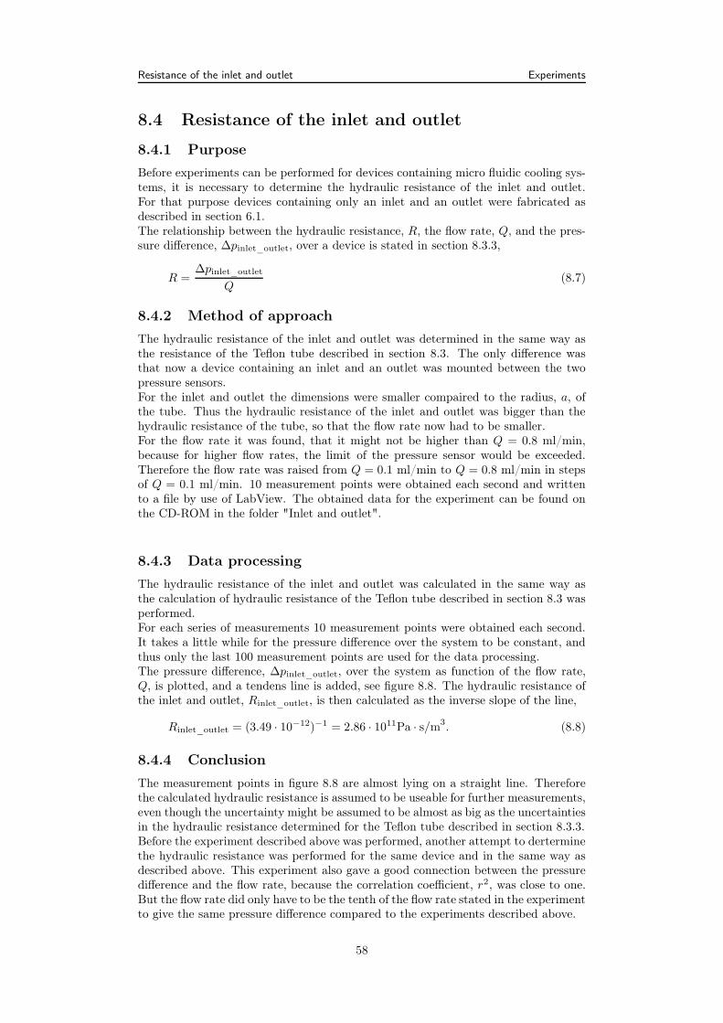
Resistance of the inlet and outlet Experiments
8.4 Resistance of the inlet and outlet
8.4.1 Purpose
Before experiments can be performed for devices containing micro fluidic cooling sys-tems, it is necessary to determine the hydraulic resistance of the inlet and outlet.For that purpose devices containing only an inlet and an outlet were fabricated asdescribed in section 6.1.The relationship between the hydraulic resistance, R, the flow rate, Q, and the pres-sure difference, ∆pinlet_outlet, over a device is stated in section 8.3.3,
R =∆pinlet_outlet
Q(8.7)
8.4.2 Method of approach
The hydraulic resistance of the inlet and outlet was determined in the same way asthe resistance of the Teflon tube described in section 8.3. The only difference wasthat now a device containing an inlet and an outlet was mounted between the twopressure sensors.For the inlet and outlet the dimensions were smaller compaired to the radius, a, ofthe tube. Thus the hydraulic resistance of the inlet and outlet was bigger than thehydraulic resistance of the tube, so that the flow rate now had to be smaller.For the flow rate it was found, that it might not be higher than Q = 0.8 ml/min,because for higher flow rates, the limit of the pressure sensor would be exceeded.Therefore the flow rate was raised from Q = 0.1 ml/min to Q = 0.8 ml/min in stepsof Q = 0.1 ml/min. 10 measurement points were obtained each second and writtento a file by use of LabView. The obtained data for the experiment can be found onthe CD-ROM in the folder "Inlet and outlet".
8.4.3 Data processing
The hydraulic resistance of the inlet and outlet was calculated in the same way asthe calculation of hydraulic resistance of the Teflon tube described in section 8.3 wasperformed.For each series of measurements 10 measurement points were obtained each second.It takes a little while for the pressure difference over the system to be constant, andthus only the last 100 measurement points are used for the data processing.The pressure difference, ∆pinlet_outlet, over the system as function of the flow rate,Q, is plotted, and a tendens line is added, see figure 8.8. The hydraulic resistance ofthe inlet and outlet, Rinlet_outlet, is then calculated as the inverse slope of the line,
Rinlet_outlet = (3.49 · 10−12)−1 = 2.86 · 1011Pa · s/m3. (8.8)
8.4.4 Conclusion
The measurement points in figure 8.8 are almost lying on a straight line. Thereforethe calculated hydraulic resistance is assumed to be useable for further measurements,even though the uncertainty might be assumed to be almost as big as the uncertaintiesin the hydraulic resistance determined for the Teflon tube described in section 8.3.3.Before the experiment described above was performed, another attempt to derterminethe hydraulic resistance was performed for the same device and in the same way asdescribed above. This experiment also gave a good connection between the pressuredifference and the flow rate, because the correlation coefficient, r2, was close to one.But the flow rate did only have to be the tenth of the flow rate stated in the experimentto give the same pressure difference compared to the experiments described above.
58
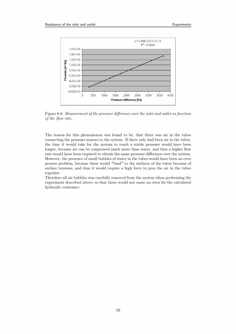
Resistance of the inlet and outlet Experiments
Figure 8.8: Measurement of the pressure difference over the inlet and outlet as functionof the flow rate.
The reason for this phenomenon was found to be, that there was air in the tubesconnecting the pressure sensors to the system. If there only had been air in the tubes,the time it would take for the system to reach a stable pressure would have beenlonger, because air can be conpressed much more than water, and thus a higher flowrate would have been required to obtain the same pressure difference over the system.However, the presence of small bubbles of water in the tubes would have been an evengreater problem, because these would "bind" to the surfaces of the tubes because ofsurface tensions, and thus it would require a high force to pres the air in the tubestogether.Therefore all air bubbles was carefully removed from the system when performing theexperiment described above, so that these would not cause an error for the calculatedhydraulic resistance.
59

Temperature measurements of a test system Experiments
8.5 Temperature measurements of a test system
8.5.1 Purpose
The first useable devices were fabricated as described in section 6.1. It was tried tosend water through the devices before experiments were performed with these. Atfirst sight it was difficult to get water all over the micro fluidic cooling systems, be-cause the some of the small and narrow channels within it remained empty, or airbubbles would occur in the structure, when water was sent through the system.Therefore, when the final devices were fabricated, a device containing at simple testsystem instead of a micro fluidic cooling system was fabricated. The structure of thetest system was one broad, twisted channel, so that the water necessarily had to fillthe whole structure, when it was flowing through the system.The water flow through the micro fluidic cooling system has to cool the upper copperplate, and the temperature has to be dependent on the flow rate, because the morewater is sent through the system, the more the system will be cooled.To obtain whelther this assumption can be applieds in practice, it is tried to measurethe temperature dependence of the flow rate.
8.5.2 Method of approach
A device containing a test system is mounted in the set-up. It is sandwiched betweenthe two copper plates, on top of the heating element, with cooling plasma betweenthe layers. The "sandwich" structure is fixed by use of a clips, and the plastic bagfilled with styrene balls is placed around it to isolate it.A glass syringe is filled with water and mounted on the squirt pump. The water havebeen poured the day before the experiment is performed to make sure that is hasroom temperature, so that then temperature of the water will not cause any mistakesduring the experiment.The syringe pump is started, and the pressure over respectively the inlet and theoutlet and the temperature of the two copper plates is measured. One measurementpoint is obtained each second, and the experiment has been performed for almost anhour, because 3603 measurement points are obtained totally. The flow rate, Q, andhence the pressure difference, ∆p, is raised during the experiment without stoppingthe water flow or the measurements. The connection between the flow rate, Q, andthe number of measurement points or the time is the following, s
Flow rate, Q Measurement points0.03 ml/min 0 to 8030.005 ml/min 804 to 17250.02 ml/min 1726 to 26800.01 ml/min 2681 to 3603
The obtained data for the experiment can be found on the CD-ROM in the folder"Test system".
8.5.3 Data processing
The output voltage from the pressure sensors and the output voltage from the temper-ature sensor are converted into resceptively a pressure and a temperature as explanedin section 7.1.2 and section 7.1.4. The pressure and the temperature is plotted asfunction of the time, see figure 8.9.From the figure it is very easy to see that the voltage measured with the pressuresensor at the inlet of the device changes, when the flow rate is changed, and thus the
60
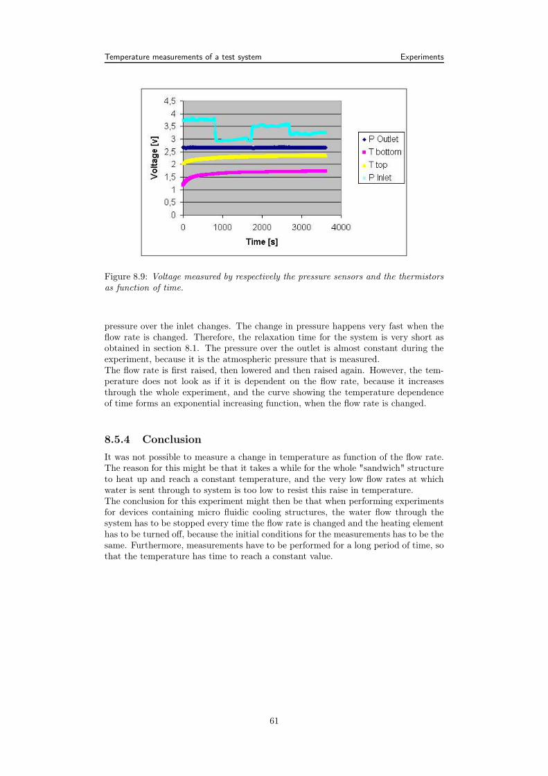
Temperature measurements of a test system Experiments
Figure 8.9: Voltage measured by respectively the pressure sensors and the thermistorsas function of time.
pressure over the inlet changes. The change in pressure happens very fast when theflow rate is changed. Therefore, the relaxation time for the system is very short asobtained in section 8.1. The pressure over the outlet is almost constant during theexperiment, because it is the atmospheric pressure that is measured.The flow rate is first raised, then lowered and then raised again. However, the tem-perature does not look as if it is dependent on the flow rate, because it increasesthrough the whole experiment, and the curve showing the temperature dependenceof time forms an exponential increasing function, when the flow rate is changed.
8.5.4 Conclusion
It was not possible to measure a change in temperature as function of the flow rate.The reason for this might be that it takes a while for the whole "sandwich" structureto heat up and reach a constant temperature, and the very low flow rates at whichwater is sent through to system is too low to resist this raise in temperature.The conclusion for this experiment might then be that when performing experimentsfor devices containing micro fluidic cooling structures, the water flow through thesystem has to be stopped every time the flow rate is changed and the heating elementhas to be turned off, because the initial conditions for the measurements has to be thesame. Furthermore, measurements have to be performed for a long period of time, sothat the temperature has time to reach a constant value.
61

Timescale measurements Experiments
8.6 Timescale measurements
8.6.1 Purpose
For the experiment performed with the PMMA plate described in section 8.2, it wasobtained that the temperature difference becomes constant after a short while, whenan isolated system is heated up. Therefore, in order to determinate for how longtime it is necessary to perform measurements on a micro fluidic cooling system beforethe temperature difference between the top and the bottom copper plate reaches aconstant level, this was proved for a device containing a micro fluidic cooling system.Furthermore, this experiment was performed in order to determine whether it is pos-sible to extrapolate the obtained results. If this is possible, the time scale for themeasurements can be lowered.
8.6.2 Method of approach
A device containing a micro fluidic cooling system optimized at ∆pcooler = 0.5 Pa,was mounted in the experimental set-up between the two pressure sensors. The microfluidic cooling system was placed between the two copper plates, on top of the heatingelement, and the whole system was fixed by use of a clips. Furthermore, the plasticback filled with styrene balls was placed around the system to isolated it from thesurroundings.Water was send through the system by use of the syringe pump. The flow rate wasfixed at Q = 0.1 ml/min = 1.67 · 10−8 m3/s during the experiment.The experiment was carried out for an hour. During the experiment, the voltageoutput obtained from the two pressure sensors and the voltage output obtained fromthe two temperature sensors were continuous measured and written to a file. Onemeasurement point was obtained each second. The obtained data for the experimentcan be found on the CD-ROM in the folder "Timescale".
8.6.3 Data processing
The voltage output obtained from the pressure sensors and the voltage output ob-tained from the two temperature sensors are plotted as a function of time, see figure8.10.
Figure 8.10: Voltage output obtained from the pressure sensors and the temperaturesensors plotted as a function of time.
62

Timescale measurements Experiments
8.6.3.1 Pressure measurements
The voltage output obtained from the two pressure sensors is plotted as function oftime is noted on figure 8.10 together with the temperature measurements.The voltage output from the two pressure sensors is converted into a pressure asdecried in section 7.1.2. As noted from figure 8.10, the magnitude of the pressuredifference is not stable through the experiment. To get an estimate of the pressuredifference, the average value of the voltage measured by the pressure sensors is calcu-lated for measurement point 100 to measurement point 3600. Thus the average totalpressure difference was calculated to be ∆ptotal = 678.3 Pa, and the standard devia-tion of this average pressure difference was calculated to be ±4.3 Pa. Calculations ofstandard deviations of average values is described in appendix 13.The pressure difference over the micro fluidic cooling system, ∆pcooler, can now becalculated from a relation between the hydraulic resistance of the cooling system,Rcooler, the resistance of the inlet and outlet, Rinlet_outlet, and the total pressuredifference over the device, ∆ptotal,
∆pcooler =
(
Rcooler
Rcooler + Rinlet_outlet
)
∆ptotal. (8.9)
The hydraulic resistance of the micro fluidic cooling system is calculated from the com-puter simulations, for which the flow rate at the inlet is calculated to be Q = 2.6 · 10−9 m3/sby taking the integral of the velocity over the inlet boundary and multiplied by theheight of the channel. The pressure difference over the cooling system was definedto be ∆pcooler = 0.5 Pa. The hydraulic resistance is then calculated from Hagen-Poiseuille’s law, see section 2.6, that states
R =∆p
Q. (8.10)
Now, the hydraulic resistance of the micro fluidic cooling system is calculated to be
Rcooler == 0.5 Pa
2.6 · 10−9 m3/s= 1.9 · 108 Pa · s/m3. (8.11)
In section 8.4 the hydraulic resistance of inlet and outlet was calculated to be Rinlet_outlet =2.9 · 1011 Pa· s/m3. The pressure difference over the micro fluidic cooling system thenbecomes
∆Pcooler =
(
1.9 · 108Pa · s/m3
1.9 · 108Pa · s/m3 + 2.9 · 1011Pa · s/m3
)
· 678, 3 Pa = 0.4 Pa,(8.12)
which is very close to the optimal pressure established for the cooling system.
8.6.3.2 Temperature measurements
The temperature output obtained from the two temperature sensors plotted as func-tion of time is noted from figure 8.10 together with the pressure measurements.The voltage output is converted into a temperature as described in section 7.1.4. Thetemperature difference of the two copper plates is then calculated and plotted as func-tion of time, note figure 8.11.As noted from the figure, there is a characteristic point around 100 s because beyondthis point the temperature difference seems to decrease exponentially. Therefore, themeasurement points beyond 100 s is fitted to an exponential function to establishwhether it is possible to extrapolate the result. The curve obtained for the fitted datais shown in figure 8.12.For the curve, the equation that the data point is fitted to is given by
y = a + b exp−x
c, (8.13)
63

Timescale measurements Experiments
Figure 8.11: Temperature difference plotted as a function of time.
Figure 8.12: Extrapolation of the temperature difference to an exponential function.
64

Timescale measurements Experiments
because this equation gives the best correlation coefficient, r2. The horizontal asymp-tote, corresponding to the temperature difference, that the system tends, is given bya, which is calculated to be 17.9C.The temperature difference that the system has reached is found by calculating the av-erage of data point 1000 to data point 3600. The temperature difference now becomes17.9C, with a standart deviation of the average temperature of ±2.4C.
8.6.4 Conclusion
The results of the experiment showed that the temperature difference of the systemwas 17.9± 2.4C. When the measurements from data point 100 to 3600 was fitted toan exponential function, the asymptote for the function was a = 17.9C which is thetemperature that the system will tend.The temperature difference that the system has reached was found from the averageof measurement point 1000 to measurement point 3600 to be 17.9 ± 2.4C, which isalmost the same as the extrapolated result.The standart derivation of the calculated average temperature is relatively high. Thereason for the relatively high standart derivation this is that the temperature differ-ence starts to increase when the experiment is almost finished. Thus, if the averageof the temperature is calculated from measurement point 1000 to measurement point1800 instead af measurement point 3600, the average temperature difference becomes17.9C, with a standard derivation of ±0.8.There is a good agreement between the measured result and the result found byextrapolation. Therefore it might be concluded that the time scale at which themeasurements is carried out has to be 1000 s, because it is only necessary to obtainedmeasurements for 1000 s before a final temperature difference of the two copper platescan be established. Furthermore it can be concluded that it is possible to extrapolatethe results and obtain a precise temperature difference for the two copper plates.
65

Temperature measurements of the micro fluidic cooling systems Experiments
8.7 Temperature measurements of the micro fluidic
cooling systems
8.7.1 Purpose
As established for the experiment described in section 8.6.1, the time scale has to be1000 s ≈ 17 min at least.This experiments are carried out to determinate the temperature difference of thetwo copper plates for two different micro fluidic cooling systems placed between theplates. For the first cooling system, the pressure difference over the inlet and outletof it is optimized for ∆pcooler = 0.5 Pa, and for the other cooling system, the pressuredifference over the inlet and outlet of it is optimized for ∆pcooler = 2.5 Pa.The two micro fluidic cooling systems are chosen because they are optimized forrelatively different pressures. The cooling system optimized for ∆pcooler =2.5 Pa arethe one of all the optimized systems, where the pressure difference could be raisedmost, without having any unphysical channels that ends blind.The temperature corresponding to the optimal pressures of the two systems has tobe measured. For both systems, the average temperature difference is determinedcorresponding to the pressure differences ∆pcooler = 0.5 Pa and ∆pcooler = 2.5 Pa.The obtained results are compared to each other.
8.7.2 Method of approach
The pressure difference, ∆pcooler, mentioned in the previous section, is the pressuredifference over a micro fluidic cooling system. However, the pressure difference mea-sured in this experiment, ∆ptotal, is the pressure difference over the whole device,including the pressure difference over the inlet and outlet.The pressure difference over a micro fluidic cooling system is determined from theequation 8.9,
∆pcooler =
(
Rcooler
Rcooler + Rinlet_outlet
)
∆ptotal. (8.14)
To obtain the decided pressure difference over the cooling system, it is necessary tochange the flow rate until the total pressure difference over the device results in thedecided pressure.The hydraulic resistance for the two cooling systems differ. Therefore, the flow ratefor the two systems has to be different.The method for the data collection is the same as described in section 8.6.2. However,before the measurements of the temperature can be performed, the pressure differenceresulting in the desired pressure difference over the cooling systems is determined.The pressure difference is changed by changing the flow rate, and then the pressuredifference is measured. This process is repeated until the desired pressure differenceis obtained. Then the heating element is turned on.The measurements were carried out for about 30 min, even though is has been obtainedin the previous section that it is only necessary to perform the experiments for 1000s. One measurement point was obtained each second, and the voltage from the twopressure sensors and the voltage from the two temperature sensors were continuouslymeasured and written to a file. The obtained data for the experiment can be foundon the CD-ROM in the folder "Temperature".
8.7.3 Data processing
The data processing is split up into two sections. The first section describes the exper-imental result obtained for the micro fluidic cooling system optimized for ∆coolerp =0.5 Pa and the second section describes experimental results obtained for the systemoptimized for ∆p = 2.5 Pa
66

Temperature measurements of the micro fluidic cooling systems Experiments
Figure 8.13: Voltage output meassured from the pressure sensores and the temperaturesensores as a function of time, for flow rate Q = 0.05ml/min
Figure 8.14: Voltage output meassured from the pressure sensores and the temperaturesensores as a function of time, for flow rate Q = 0.5ml/min
8.7.3.1 Micro fluidic cooling system optimized for 0.5 Pa
The flow rate, Q, that results in the desired pressure difference, ∆p = 0.5 Pa, overthe micro fluidic cooling system is found to be around Q = 0.05 ml/min. Similar, theflow rate that results in a pressure difference of ∆p = 2.5 Pa is found to be aroundQ = 0.5 ml/min.For the flow rate Q = 0.05 ml/min the measurements are carried out in 30 min.The voltage measured from two pressure sensors and the voltage measured from thetemperature sensors are plotted as function of time, see figure 8.13.For the flow rate Q = 0.5 ml/min the measurements are carried out in 17 min. Thevoltage measured from the two pressure sensors and the voltage measured from thetemperature sensors are plotted as function of the time, see figure 8.14.
8.7.3.2 Pressure measurements
The output voltage measured by the pressure sensors is converted into a pressure asdescribed in section 7.1.2.The average pressure difference, ∆p, over the device is calculated by determining theaverage value of the measurement point 100 to the last measurement point.
67

Temperature measurements of the micro fluidic cooling systems Experiments
The average of the pressure difference, ∆p, and the standard derivation of the averagepressure difference, ±∆p, for the two flow rates, Q, are calculated, and the pressuredifference, ∆pcooler, for the cooling system are calculated from equation 8.9. Theresults of the calculations are noted in table 8.1.As noted from table 8.1, the pressure difference over the micro fluidic cooling system
Q ∆p ±∆p ∆pcooler
0.05 ml/min 1110.8 Pa ±4.7 Pa 0.7 Pa0.5 ml/min 3864.5 Pa ±1 Pa 2.5 Pa
Table 8.1: Pressure difference, ∆p, standard derivation of the average pressure dif-ference, ±∆p, and the pressure difference over the cooler, ∆pcooler, at different flowrates, Q. The micro fluidic cooling system is optimized for ∆pcooler=0.5 Pa
is almost corresponding to the desired pressure difference for both flow rates.
8.7.3.3 Temperature measurements
The output voltage measured from the two temperature sensors are converted into atemperature as described in section 7.1.4.The temperature differences obtained for the system at the two flow rates are deter-mined by the calculating the average from measurement point 1000 to the last datapoint. This is done in order to estimate the final temperature difference.To extrapolate the average temperature, the data points from 100 to the last datapoint is fitted to an exponential function. The exponential function is given by
y = a + b exp−x
c, (8.15)
where a determines the asymptote, which corresponds to the temperature, ∆Texp,that the average temperature of the system will tend. Furthermore, the temperature,∆T , estimated from measurement point 1000 to the last measurement point and thestandard derivation of the average temperature, ±∆T , is calculated. The results ofthe calculations are shown in table 8.2.A figure showing the temperature difference plotted as function of the time and a
Q ∆T ±∆T ∆Texp
0.05ml/min 18.5C ±0.002C 18.5C0.5ml/min 19.6C ±0.009C 19.4C
Table 8.2: Average temperature, ∆T , standart derivation of the average temperature,±∆T , and the extrapolated temperature difference, ∆Texp, at difference flow rates, Q.The micro fluidic cooling system is optimized for ∆pcooler = 0.5Pa
figures for the fitted data is noted in figure 8.15.
8.7.3.4 Micro fluidic cooling system optimized for 2.5 Pa
The flow rate that gives the desired pressure difference over the micro fluidic coolingsystem, at ∆pcooler = 0.5 Pa is around Q = 0.05 ml/min, while the flow rate thatgives a pressure difference of ∆pcooler = 2.5 pa is around 0.2 textrmml/min.For the flow rate Q = 0.05 ml/min the measurements are carried out for 30 min. Thevoltage measured from the two pressure sensors and the voltage measured from thetwo temperature sensors are plotted as function of time, see figure ??.For the flow rate Q = 0.2 ml/min, the measurements are carried out for 30 min. Thevoltage measured from the two pressure sensors and the voltage measured from thetemperature sensors are plotted as function of time, see figure 8.18(a).
68

Temperature measurements of the micro fluidic cooling systems Experiments
(a) The temperature difference for a systemoptimized for ∆pcooler = 0.5ml/min, forQ = 0.05ml/min
(b) The extrapolated temperature differencefor a system optimized at ∆pcooler =0.5 Pa,for Q = 0.05 ml/min
(c) The temperature difference for a systemoptimized at ∆pcooler = 0.5ml/min, for Q =
0.5ml/min
(d) The extrapolated temperature differencefor a system optimized at ∆pcooler =0.5 Pa,for Q = 0.5 ml/min
Figure 8.15: The average temperature for a system optimized at ∆pcooler = 0.5Pa
8.7.3.5 Pressure measurements
The average of the pressure difference over the device, ∆p, the standart derivation ofthe average pressure over the device, ±∆p, and the pressure difference over the microfluidic cooling system, ∆pcooler, are calculated as described in section ??. The resultsof the calculations are shown in table 8.3.As noted from table 8.3, is the calculated pressure difference obtained for both flow
Q ∆p ±∆p ∆pcooler
0.05 ml/min 574.34 Pa ±4.9 Pa 0.5 Pa0.2 ml/min 2756.5 Pa ±4.1 Pa 2.3 Pa
Table 8.3: Pressure difference, ∆p, standart derivation of the average pressure dif-ference, ±∆p, and the pressure difference over the cooler, ∆pcooler, at different flowrates, Q. The micro fluidic cooling system is optimized for ∆pcooler = 2.5Pa
rates almost corresponding to the desired pressure differences.
8.7.3.6 Temperature measurements
The average temperature of the micro fluidic cooling system, ∆T , the standart deriva-tion from the average temperature, ±∆T , and the extrapolated temperature, ∆Texp,are calculated as described in section 8.7.3.3. The results of the calculations are shownin table 8.4A figure showing the temperature difference plotted as function of the time and a
figures for the fitted data is noted in figure 8.18.
69

Temperature measurements of the micro fluidic cooling systems Experiments
Figure 8.16: Voltage output meassured from the pressure sensores and the temperaturesensores plottet as a function of time, for flow rate Q = 0.05ml/min
Figure 8.17: The voltage output meassured from the pressure sensores and the tem-perature sensores as a function of time, for flow rate Q = 0.2ml/min
70

Temperature measurements of the micro fluidic cooling systems Experiments
Q ∆T ±∆T ∆Texp
0.05 ml/min 17.8C ±0.002C 17.8C0.2 ml/min 19.2C ±0.003C 19.3C
Table 8.4: Temperature, ∆T , standart derivation of the temperature difference, ±∆T ,and the extrapolated temperature difference, at different flow rates, Q. The microfluidic cooling system is optimized for ∆pcooler = 2.5Pa
(a) The temperature difference for a systemoptimezed at ∆pcooler = 2.5ml/min, for Q =
0.05ml/min
(b) The extrapolated temperature differencefor a system optimezed at ∆pcooler = 2.5Pa,for Q = 0.05 ml/min
(c) The temperature difference for a systemoptimezed at ∆pcooler = 2.5ml/min, for Q =
0.5ml/min
(d) The extrapolated temperature differencefor a system optimezed at ∆pcooler =
2.5ml/min, for Q = 0.2ml/min
Figure 8.18: The average temperature for a system optimized at ∆pcooler = 2.5Pa
8.7.4 Conclusion
The experimental obtained temperature differences and pressure differences for thetwo micro fluidic cooling systems, the standart derivation of the average temperatureand the extrapolated temperatures for the two systems are noted in table 8.5.
System 0.5 System 2.5∆pcooler ∆T ±∆T ∆Texp ∆pcooler ∆T ±∆T ∆Texp
0.7Pa 18.5C ±0.002C 18.5C 0.5Pa 17.8C ±0.002C 17.8C2.5Pa 19.6C ±0.009C 19.4C 2.3Pa 19.2C ±0.003C 19.3C
Table 8.5: Temperature, ∆T , standart derivation of the average temperature, ±∆T ,and the extrapolated temperature difference ∆Texp, at different pressure differencesover the micro fluidic cooling system, ∆pcooler. The two micro fluidic cooling systemsare optimized for ∆pcooler =0.5 Pa and ∆pcooler=2.5 Pa, respectively.
From table 8.5 it is noted, that the temperature is measured with very high accuracy,
71
Temperature measurements of the micro fluidic cooling systems Experiments
because the standard deviation of the average is very low. Furthermore, it is notedthat for the system optimized for ∆pcooler = 2.5 Pa, the lowest temperature is ob-tained for both measurements performed with this device.The measurements are carried out over a relatively long period of time compared tothe measurement time found in the previous section, a which a constant temperaturedifference would be obtained.Although the system is isolated by a plastic bag containing styrene balls, the sur-roundings will have an influence on the measured temperature of the two systems,because the syringe balls are not able to isolate the system totally from the surround-ings. Furthermore, the experiments were carried out over two days, and thus theroom temperature could have been different while performing the experiments for thetwo different cooling systems. But also the small changed might have been presentedwithin the experimental set-up, when measurements are not performed in the sametime.The determination of the hydraulic resistance for the systems is based on the teore-tical simulation. When the device are fabricated using the CO2 laser, the structuresof the micro fluidic cooling system is broaden a bit. Therefore, the hydraulic resistantfor the actual system might be lower than the hydraulic resistance corresponding tothe value of ∆pcooler used within the optimizations. Furthermore, when fabricatingthe devices, the dimensions of the inlet and outlet channels may differ a bit for thedevices, because of uncertainties within the laser set-up.The hydraulic resistance of the micro fluidic cooling system and of the inlet and outletwas only determined once. Therefore, it might have been determined with a greatuncertainty. The uncertainty of the total pressure difference becomes relatively highso the pressure difference over the micro fluidic cooling system is neither very accu-rate. Is it a fact that the pressure difference over the micro fluidic cooling systems isproportional to the flow rate. Therefore the pressure difference increases as the flowrate increases, and thus the temperature difference increases.In the previous experiment the average temperature of the micro fluidic cooling systemoptimized for ∆pcooler = 0.5 Pa was determined to be ∆T = 17.9±2.4C. The pressuredifference over the micro fluidic cooling system then calculated to be ∆pcooler = 0.4 Pa.The pressure difference obtained in this experiment was ∆p = 0.7Pa and the calcu-lated average temperature difference was ∆T = 18.5. Therefore, the temperaturedifference increases as the pressure difference increases, which is in agreement withthe theory, because when the pressure difference is increased the flow rate is increasedand more water is flowing through the cooling system. When more water is flowingthrough the cooling system, more heat can be conducted away from the it.If only the temperatures obtained for the system for which the pressure different wasapproximately ∆pcooler = 2.5Pa are considered, the lowest temperature obtained forthis system is lowest average temperature. Therefore it is the most optimal coolingsystem at ∆pcooler = 2.5 Pa.The extrapolated temperatures for the average temperature of the micro fluidic cool-ing systems are in agreement with the average temperatures.Unfortunately, the experiments were not repeated because of lack of time, and thetherefore it is not known whether the results can be reproduced or not.
72
Chapter 9
Conclusion
The main purpose of the present project was to perform topology optimizations ofmicro fluidic cooling systems and to fabricate the systems in PMMA using a CO2
laser.The optimizations were carried out for several geometries. The final geometry waschosen as a rectangle and the whole design area was heated. The structure wasoptimized for different pressures. The results showed that the systems were optimalfor low pressure differences between inlet and outlet. However, when the pressuredifference was increased, the structures were no longer optimal compared to a systemoptimized at a different pressure. The reason for this might be that the optimizationis performed numerically and therefore the optimization can only be as accurate asthe number of points at which the solution is calculated.When the pressure difference between the inlet and outlet is increased, the number ofchannels that terminates within the solid material is increased. This is not a physicallyacceptable solution to the optimization problem. However, it is found that decreasingthe width of the inlet and outlet leads to an increase of the pressure difference atwhich the channels start to terminate in the solid.Heat conduction experiments though a PMMA plate were carried out and the resultclearly showed that the system had to be isolated from the surroundings.Also investigated is the resistance of a tube having well-defined dimensions and theresult is compared to the theoretically calculated resistance of such a tube. The resultis used to estimate the precision that can be obtained for the hydraulic resistance ofthe inlet and outlet part of the micro fluidic system. The hydraulic resistance of thetube was measured twice, and the measurements that gave the largest coefficient ofcorrelation resulted in a deviation from the theoretical result of 33.1 %. Therefore itwas assumed that the hydraulic resistance for the inlet and outlet can be measuredto an accuracy of approximately 33 %. The resistance of the inlet and outlet is usedto calculate the pressure difference between the inlet and outlet of the system.Furthermore, an experiment is carried out to establish the time needed to obtainreasonable results for the average temperature. The time scale is establish to be 1000s, and it is shown that at this time scale the average temperature of the system canbe extrapolated.Two systems were fabricated, one system with the optimal pressure difference 2.5 Pa,and one system with the optimal pressure difference 0.5 Pa.Measurements were carried out to establish the average temperature for each of thesystems at 0.5 Pa respectively 2.5Pa.The average temperature for the system optimized at 2.5 Pa was the lower at bothpressure differences, 0.5 Pa and 2.5 Pa. Therefore the optimized system might not bethe most optimal.
73
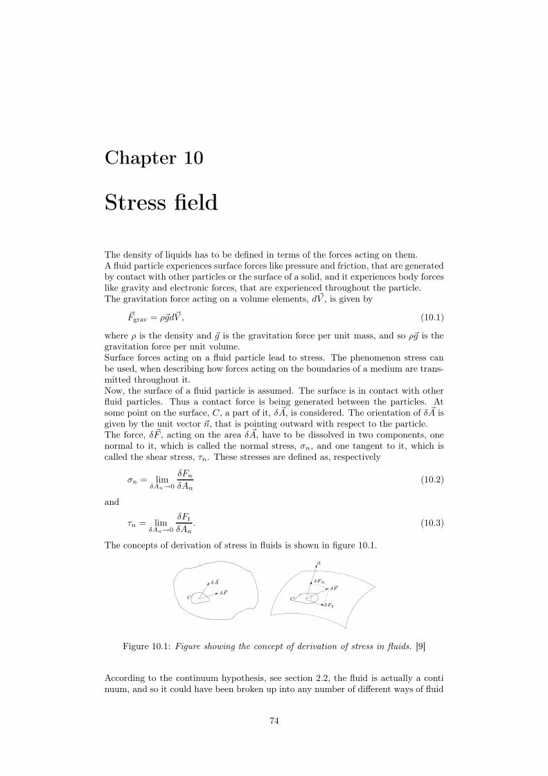
Chapter 10
Stress field
The density of liquids has to be defined in terms of the forces acting on them.A fluid particle experiences surface forces like pressure and friction, that are generatedby contact with other particles or the surface of a solid, and it experiences body forceslike gravity and electronic forces, that are experienced throughout the particle.The gravitation force acting on a volume elements, d~V , is given by
~Fgrav = ρ~gd~V , (10.1)
where ρ is the density and ~g is the gravitation force per unit mass, and so ρ~g is thegravitation force per unit volume.Surface forces acting on a fluid particle lead to stress. The phenomenon stress canbe used, when describing how forces acting on the boundaries of a medium are trans-mitted throughout it.Now, the surface of a fluid particle is assumed. The surface is in contact with otherfluid particles. Thus a contact force is being generated between the particles. Atsome point on the surface, C, a part of it, δ ~A, is considered. The orientation of δ ~A isgiven by the unit vector ~n, that is pointing outward with respect to the particle.The force, δ ~F , acting on the area δ ~A, have to be dissolved in two components, onenormal to it, which is called the normal stress, σn, and one tangent to it, which iscalled the shear stress, τn. These stresses are defined as, respectively
σn = limδAn→0
δFn
δAn(10.2)
and
τn = limδAn→0
δFt
δAn. (10.3)
The concepts of derivation of stress in fluids is shown in figure 10.1.
~n
δ ~F
δFn
C
δFt
δ ~A
Cδ ~F
Figure 10.1: Figure showing the concept of derivation of stress in fluids. [9]
According to the continuum hypothesis, see section 2.2, the fluid is actually a continuum, and so it could have been broken up into any number of different ways of fluid
74

Stress field
particles around the point C, and therefore obtained any different number of stressesat this point. [9]
75

Chapter 11
Viscosity
A steady-state flow is laminar and can be split-up into layers that flow parallel toeach other, which also will mentioned in section 2.3.The flow of a liquid will never occur without friction, even though this often is as-sumed, because the layers in the laminar flow "rub" against each other, while they arenot moving with the same velocity. Or it could be said that if a liquid is influencedby a shear stress, it begins to yield. The magnitude of the friction is different fordifferent liquids and can be describes by the viscosity of the liquid.
F
z
x
τ
A
A
u
Figure 11.1: Figure for derivation of viscosity showing two parallel plates, where onof them is moving with a constant velocity, u. A liquid is flowing between the plateswith a laminar flow.
A liquid flowing between two parallel plates is assumed, where on of the plates is mov-ing in the x direction with a constant velocity, u, so that the plates remain parallelto each other as shown in figure 11.1. The distance between the plates is h.The force, F , that the plate in motion has to be influenced by is proportional to itssize, A, and to the velocity, u, and inverse proportional to the distance between theplates, h,
F = ηu
hA. (11.1)
The constant of proportionality is the viscosity, η, that for water is 0.001 mPa·s. Theviscosity can be explained as being the resistance against yield for fluids.If a thin parallel layer between the plates is considered instead of the entire space,the same tangential forces are represented, because of Newton’s third law,
τn = η∂ux
∂z, (11.2)
76

Viscosity
where τn is the shear stress. The directions x and z are shown in figure 11.1.Liquids satisfying the equation 11.2 and which are independent of the shear stress aretermed Newtonian fluids. [8]
77

Chapter 12
Derivation of the Péclet number
The Péclet number can be derived from an expression for the dimensionsless heatequation used in the FEMLab application mode and derived in section 2.8.2 for anincompressible fluid in steady-state,
ρC~u~∇T + ~∇(k~∇T ) = Q (12.1)m
ρC~u~∇T − k~∇2T ) = Q (12.2)
The velocity vector has both a component in the x and in the y direction, so that~u = [vx, vy]. Thus if the fluid is moving in the x direction, the velocity in the ydirection is 0, vy = 0. Thus
vxρC∂T
∂x= Q + k ~∇2T. (12.3)
Now expressions in term of dimensionless number are introduced as follows
x = Lx y = Ly t = t0t T = T0T . (12.4)
If the fluid is moving in the x-direction, it is possible to make the velocity in thisdirection, ux, dimensionsless by use of the chain rule,
v =∂x
∂t=
∂x
∂x
∂x
∂t
∂t
∂t=
L
t0
∂x
∂t= v0v. (12.5)
Inserting the expression for the velocity in the expression 12.3 gives
u0uρC∂T
∂x= Q + k~∇2T. (12.6)
Rewriting the dimensionless numbers and interting gives
u0uρCT0
L
∂T
∂x= Q + k
T0
L2~∇2T (12.7)
Dividing by k T0
L2 gives
u0ρCL
kv∂T
∂x=
L2
kT0Q + ~∇2T . (12.8)
The Péclets number is known to be defined as
Pe =u0ρCL
k(12.9)
Then the final expression becomes [6]
Pe · u∂T
∂x=
L2
kT0Q + ~∇2T . (12.10)
78

Chapter 13
Calculation of standard
derivations
For an amount of measurement points, the average is calculated from
x =1
N
N∑
i=1
xi, (13.1)
where N is the number of measurements and xi is the i’the measurement. The averageuncertainty of the individual measurements, x1, x2, x3, ...., xN , is then given by thestandard deviation
αx =
√
1
N − 1
∑
(xi − x)2. (13.2)
This equation states the sample standard derivation. The significance of the standarddeviation, αx, is that approximately 68% of the measurements of x shave to lie withina distance αx of the true value.As long as the systematic uncertainties are negligible, the uncertainty of the averageis the standard derivation of the average [25],
αx =αx√N
, (13.3)
which is the equation used when calculating standard derivations of experimentalresults obtained in this project.
79

Chapter 14
Data sheets for pressure sensors
and temperature sensors
80

References
[1] Teoretical microfluics, Henrik Bruus, MIC, DTU 2004
[2] Transport Phenomena, R. Byron and others, John Wiley & Sons, 2nd edition,2002
[3] Microstructure fabrication with a CO2 laser system, Deflef Snakenborg with oth-ers, MIC, DTU, 2003
[4] Nano 1 - Introduction to Nanotechnology, Henrik Bruus, MIC, DTU 2004
[5] section1: Fluid Michanics and Fluid Properties, http://www.efm.leeds.ac.uk-/CIVE/CIVE1400/Section1/Fluid_mechanics.htm
[6] Topologioptimering, Katrine Andersen with others, MIC, DTU, January 2005
[7] http://mmf.ruc.dk/ jogvan/Speciale/speciale.pdf, Stine Marott Normann withothers, RUC
[8] Mekanik, Gunnar Christiansen and others. Institut for Fysik, DTU, 2000
[9] Introduction to Fluid Mechanics, sixth edition, Robert W. Fox and others, JohnWiley and Sons, Inc., 2004
[10] Moshe B. Fuchs, Department of Solid Mechanics, Materials and Systems, TelAviv University, Israel, 2002
[11] Stoftransport i planter og porøse stoffer, Lars Øgendahl, KVL, 2004
[12] a high-level programming-language implementation of topology optimizationaplied to steady-state Navier-Stokes flow, Laurits Højgaard Olesen and others,MIC, DTU, 2004
[13] NTC Termistors, Bowthorpe Thermoelectronics, UK
[14] www.betatherm.com/datasheet.php?p_id=90, Micro BetaCHIP Probe (MCD)
[15] Understanding the Finite Element Method, documentation, FEMLab 3.1
[16] Using The PDE Modes, documentation, FEMLab 3.1
[17] Setup of TOPOPT S-problem using FEMLAB-GUI, Fridolin Okkels, MIC, DTU
[18] The Conduction and Convection Application Mode, documentation, FEMLab3.1
[19] The Navier-Stokes Application Mode, documentation, FEMLab 3.1
[20] Transport Phenomea. second edition, R. Byron Bird and others, 2002
[21] http://hyperphysics.phy-astr.gsu.edu/hbase/thermo/heatra.html
81

REFERENCES REFERENCES
[22] Physics of Continuos Matter, Exotic and Everyday Phenomena in the Micro-scopic World, Benny Lautrup, 2005
[23] http://www.efunda.com/formulae/heat_transfer/conduction/overview_cond.cfm
[24] Heat tranfer, Femlab Modeling Guide, FEMLab 3.1
[25] An Introducuction To Error Analyses, second edition, John R. Taylor, UniversityScience Books, 1997
82