torque diagram and torsional stress of circular section of solids ii.pdf · 1 torque diagram and...
TRANSCRIPT
1
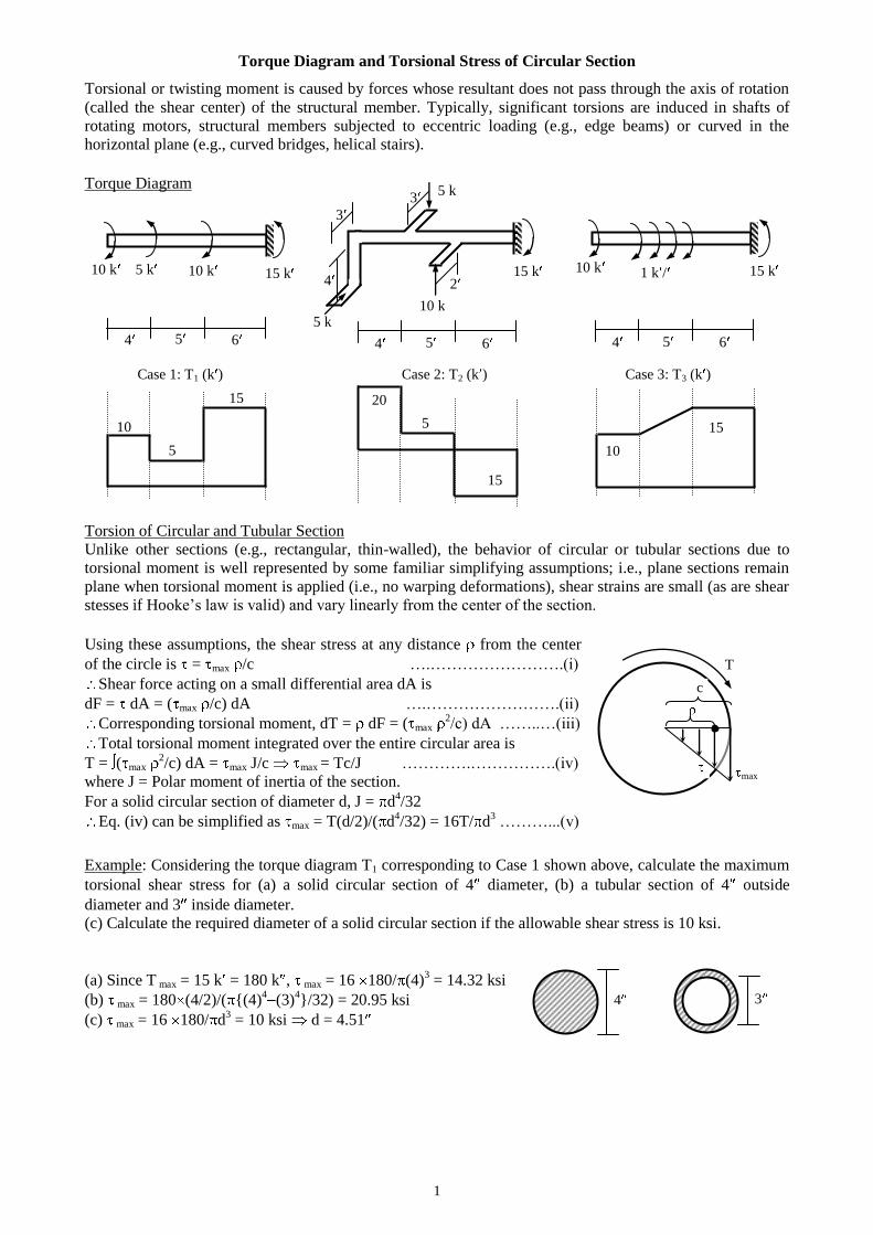
Torque Diagram and Torsional Stress of Circular Section
Torsional or twisting moment is caused by forces whose resultant does not pass through the axis of rotation
(called the shear center) of the structural member. Typically, significant torsions are induced in shafts of
rotating motors, structural members subjected to eccentric loading (e.g., edge beams) or curved in the
horizontal plane (e.g., curved bridges, helical stairs).
Torque Diagram
Case 1: T1 (k ) Case 2: T2 (k ) Case 3: T3 (k )
Torsion of Circular and Tubular Section
Unlike other sections (e.g., rectangular, thin-walled), the behavior of circular or tubular sections due to
torsional moment is well represented by some familiar simplifying assumptions; i.e., plane sections remain
plane when torsional moment is applied (i.e., no warping deformations), shear strains are small (as are shear
stesses if Hooke’s law is valid) and vary linearly from the center of the section.
Example: Considering the torque diagram T1 corresponding to Case 1 shown above, calculate the maximum
torsional shear stress for (a) a solid circular section of 4 diameter, (b) a tubular section of 4 outside
diameter and 3 inside diameter.
(c) Calculate the required diameter of a solid circular section if the allowable shear stress is 10 ksi.
(a) Since T max = 15 k = 180 k , max = 16 180/ (4)3 = 14.32 ksi
(b) max = 180 (4/2)/( {(4)4
(3)4}/32) = 20.95 ksi
(c) max = 16 180/ d3 = 10 ksi d = 4.51
3
T
max
c
5 k 10 k
15 k 10 k 1 k / 15 k
5 k
10 k 5 k 10 k 15 k
4 5 6 4 5 6
3
2
4 5 6
10
5
15 20
5
15
10
15
Using these assumptions, the shear stress at any distance from the center
of the circle is = max /c ….…………………….(i)
Shear force acting on a small differential area dA is
dF = dA = ( max /c) dA ….…………………….(ii)
Corresponding torsional moment, dT = dF = ( max 2/c) dA ……..…(iii)
Total torsional moment integrated over the entire circular area is
T = ( max 2/c) dA = max J/c max = Tc/J ………….…………….(iv)
where J = Polar moment of inertia of the section.
For a solid circular section of diameter d, J = d4/32
Eq. (iv) can be simplified as max = T(d/2)/( d4/32) = 16T/ d
3 ………...(v)
4
4 3
2
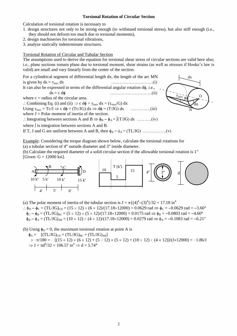
Torsional Rotation of Circular Section
Calculation of torsional rotation is necessary to
1. design structures not only to be strong enough (to withstand torsional stress), but also stiff enough (i.e.,
they should not deform too much due to torsional moments),
2. design machineries for torsional vibrations,
3. analyze statically indeterminate structures.
Torsional Rotation of Circular and Tubular Section
The assumptions used to derive the equation for torsional shear stress of circular sections are valid here also;
i.e., plane sections remain plane due to torsional moment, shear strains (as well as stresses if Hooke’s law is
valid) are small and vary linearly from the center of the section.
where is integration between sections A and B.
If T, J and G are uniform between A and B, then B A = (TL/JG) …………….(v)
Example: Considering the torque diagram shown below, calculate the torsional rotations for
(a) a tubular section of 4 outside diameter and 3 inside diameter.
(b) Calculate the required diameter of a solid circular section if the allowable torsional rotation is 1
[Given: G = 12000 ksi].
(a) The polar moment of inertia of the tubular section is J = {(4)4
(3)4}/32 = 17.18 in
4
D C = (TL/JG)CD = (15 12) (6 12)/(17.18 12000) = 0.0629 rad C = 0.0629 rad = 3.60
C B = (TL/JG)BC = (5 12) (5 12)/(17.18 12000) = 0.0175 rad B = 0.0803 rad = 4.60
B A = (TL/JG)AB = (10 12) (4 12)/(17.18 12000) = 0.0279 rad A = 0.1083 rad = 6.21
(b) Using D = 0, the maximum torsional rotation at point A is
A = [(TL/JG)CD + (TL/JG)BC + (TL/JG)AB]
/180 = [(15 12) (6 12) + (5 12) (5 12) + (10 12) (4 12)]/(J 12000) = 1.86/J
J = d4/32 = 106.57 in
4 d = 5.74
T (k )
O
N
M
1
max
d
For a cylindrical segment of differential length dx, the length of the arc MN
is given by ds = max dx ….…………………….(i)
It can also be expressed in terms of the differential angular rotation d , i.e.,
ds = c d ….…………………….(ii)
where c = radius of the circular area.
Combining Eq. (i) and (ii) c d = max dx = ( max/G) dx
Using max = Tc/J c d = (Tc/JG) dx d = (T/JG) dx ………..…(iii)
where J = Polar moment of inertia of the section.
Integrating between sections A and B B A = (T/JG) dx ……….(iv)
4
dx
4 5 6
D C
A
B
10 k 5 k 10 k 15 k
d 3 10
5
15
3
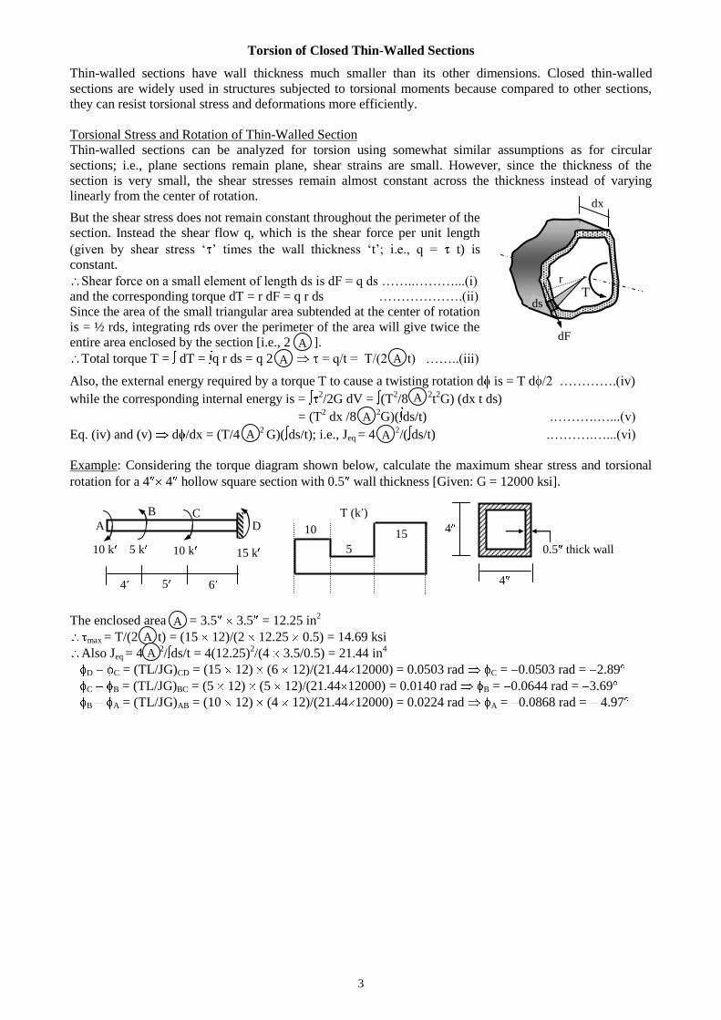
Torsion of Closed Thin-Walled Sections
Thin-walled sections have wall thickness much smaller than its other dimensions. Closed thin-walled
sections are widely used in structures subjected to torsional moments because compared to other sections,
they can resist torsional stress and deformations more efficiently.
Torsional Stress and Rotation of Thin-Walled Section
Thin-walled sections can be analyzed for torsion using somewhat similar assumptions as for circular
sections; i.e., plane sections remain plane, shear strains are small. However, since the thickness of the
section is very small, the shear stresses remain almost constant across the thickness instead of varying
linearly from the center of rotation.
Also, the external energy required by a torque T to cause a twisting rotation d is = T d /2 ………….(iv)
while the corresponding internal energy is = 2/2G dV = (T
2/8
2t2G) (dx t ds)
= (T2 dx /8
2G)( ds/t) .……….…...(v)
Eq. (iv) and (v) d /dx = (T/4 2 G)( ds/t); i.e., Jeq = 4
2/( ds/t) .……….…...(vi)
Example: Considering the torque diagram shown below, calculate the maximum shear stress and torsional
rotation for a 4 4 hollow square section with 0.5 wall thickness [Given: G = 12000 ksi].
The enclosed area = 3.5 3.5 = 12.25 in2
max = T/(2 t) = (15 12)/(2 12.25 0.5) = 14.69 ksi
Also Jeq = 4 2/ ds/t = 4(12.25)
2/(4 3.5/0.5) = 21.44 in
4
D C = (TL/JG)CD = (15 12) (6 12)/(21.44 12000) = 0.0503 rad C = 0.0503 rad = 2.89
C B = (TL/JG)BC = (5 12) (5 12)/(21.44 12000) = 0.0140 rad B = 0.0644 rad = 3.69
B A = (TL/JG)AB = (10 12) (4 12)/(21.44 12000) = 0.0224 rad A = 0.0868 rad = 4.97
T (k )
But the shear stress does not remain constant throughout the perimeter of the
section. Instead the shear flow q, which is the shear force per unit length
(given by shear stress ‘ ’ times the wall thickness ‘t’; i.e., q = t) is
constant.
Shear force on a small element of length ds is dF = q ds ……..………...(i)
and the corresponding torque dT = r dF = q r ds ……………….(ii)
Since the area of the small triangular area subtended at the center of rotation
is = ½ rds, integrating rds over the perimeter of the area will give twice the
entire area enclosed by the section [i.e., 2 ].
Total torque T = dT = q r ds = q 2 = q/t = T/(2 t) ……..(iii)
4 10
5
15
4 5 6
D C
A
B
10 k 5 k 10 k 15 k
4
dx
T ds
dF
r
A
A
A
A
A A
A
0.5 thick wall
A
A
A
4
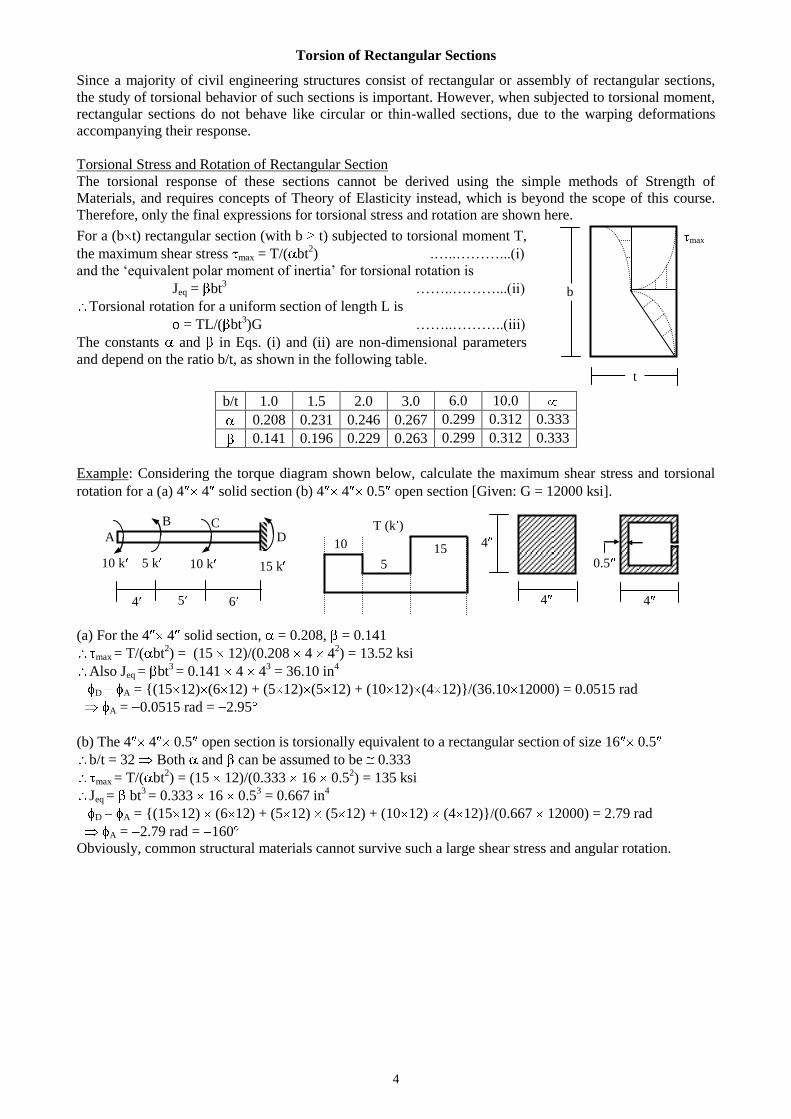
Torsion of Rectangular Sections
Since a majority of civil engineering structures consist of rectangular or assembly of rectangular sections,
the study of torsional behavior of such sections is important. However, when subjected to torsional moment,
rectangular sections do not behave like circular or thin-walled sections, due to the warping deformations
accompanying their response.
Torsional Stress and Rotation of Rectangular Section
The torsional response of these sections cannot be derived using the simple methods of Strength of
Materials, and requires concepts of Theory of Elasticity instead, which is beyond the scope of this course.
Therefore, only the final expressions for torsional stress and rotation are shown here.
b/t 1.0 1.5 2.0 3.0 6.0 10.0
0.208 0.231 0.246 0.267 0.299 0.312 0.333
0.141 0.196 0.229 0.263 0.299 0.312 0.333
Example: Considering the torque diagram shown below, calculate the maximum shear stress and torsional
rotation for a (a) 4 4 solid section (b) 4 4 0.5 open section [Given: G = 12000 ksi].
(a) For the 4 4 solid section, = 0.208, = 0.141
max = T/( bt2) = (15 12)/(0.208 4 4
2) = 13.52 ksi
Also Jeq = bt3 = 0.141 4 4
3 = 36.10 in
4
D A = {(15 12) (6 12) + (5 12) (5 12) + (10 12) (4 12)}/(36.10 12000) = 0.0515 rad
A = 0.0515 rad = 2.95
(b) The 4 4 0.5 open section is torsionally equivalent to a rectangular section of size 16 0.5
b/t = 32 Both and can be assumed to be 0.333
max = T/( bt2) = (15 12)/(0.333 16 0.5
2) = 135 ksi
Jeq = bt3 = 0.333 16 0.5
3 = 0.667 in
4
D A = {(15 12) (6 12) + (5 12) (5 12) + (10 12) (4 12)}/(0.667 12000) = 2.79 rad
A = 2.79 rad = 160
Obviously, common structural materials cannot survive such a large shear stress and angular rotation.
T (k )
For a (b t) rectangular section (with b t) subjected to torsional moment T,
the maximum shear stress max = T/( bt2) .…..………...(i)
and the ‘equivalent polar moment of inertia’ for torsional rotation is
Jeq = bt3 ……..………...(ii)
Torsional rotation for a uniform section of length L is
= TL/( bt3)G ……..………..(iii)
The constants and in Eqs. (i) and (ii) are non-dimensional parameters
and depend on the ratio b/t, as shown in the following table.
4 10
5
15
4 5 6
D C
A
B
10 k 5 k 10 k 15 k
4
max
t
b
4
0.5
5
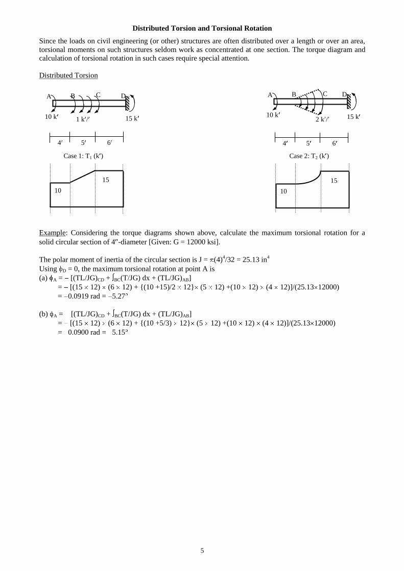
Distributed Torsion and Torsional Rotation
Since the loads on civil engineering (or other) structures are often distributed over a length or over an area,
torsional moments on such structures seldom work as concentrated at one section. The torque diagram and
calculation of torsional rotation in such cases require special attention.
Distributed Torsion
Case 1: T1 (k ) Case 2: T2 (k )
Example: Considering the torque diagrams shown above, calculate the maximum torsional rotation for a
solid circular section of 4 -diameter [Given: G = 12000 ksi].
The polar moment of inertia of the circular section is J = (4)4/32 = 25.13 in
4
Using D = 0, the maximum torsional rotation at point A is
(a) A = [(TL/JG)CD + BC(T/JG) dx + (TL/JG)AB]
= [(15 12) (6 12) + {(10 +15)/2 12} (5 12) +(10 12) (4 12)]/(25.13 12000)
= 0.0919 rad = 5.27
(b) A = [(TL/JG)CD + BC(T/JG) dx + (TL/JG)AB]
= [(15 12) (6 12) + {(10 +5/3) 12} (5 12) +(10 12) (4 12)]/(25.13 12000)
= 0.0900 rad = 5.15
D C B A D C B A
10
15
10
15
10 k 2 k / 15 k 10 k 1 k / 15 k
4 5 6 4 5 6
6
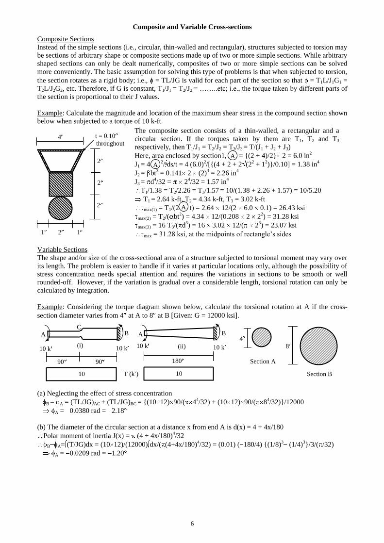
Composite and Variable Cross-sections
Composite Sections
Instead of the simple sections (i.e., circular, thin-walled and rectangular), structures subjected to torsion may
be sections of arbitrary shape or composite sections made up of two or more simple sections. While arbitrary
shaped sections can only be dealt numerically, composites of two or more simple sections can be solved
more conveniently. The basic assumption for solving this type of problems is that when subjected to torsion,
the section rotates as a rigid body; i.e., = TL/JG is valid for each part of the section so that = T1L/J1G1 =
T2L/J2G2, etc. Therefore, if G is constant, T1/J1 = T2/J2 = ……..etc; i.e., the torque taken by different parts of
the section is proportional to their J values.
Example: Calculate the magnitude and location of the maximum shear stress in the compound section shown
below when subjected to a torque of 10 k-ft.
Variable Sections
The shape and/or size of the cross-sectional area of a structure subjected to torsional moment may vary over
its length. The problem is easier to handle if it varies at particular locations only, although the possibility of
stress concentration needs special attention and requires the variations in sections to be smooth or well
rounded-off. However, if the variation is gradual over a considerable length, torsional rotation can only be
calculated by integration.
Example: Considering the torque diagram shown below, calculate the torsional rotation at A if the cross-
section diameter varies from 4 at A to 8 at B [Given: G = 12000 ksi].
(a) Neglecting the effect of stress concentration
B A = (TL/JG)AC + (TL/JG)BC = {(10 12) 90/( 44/32) + (10 12) 90/( 8
4/32)}/12000
A = 0.0380 rad = 2.18
(b) The diameter of the circular section at a distance x from end A is d(x) = 4 + 4x/180
Polar moment of inertia J(x) = (4 + 4x/180)4/32
B A= (T/JG)dx = (10 12)/(12000) dx/( (4+4x/180)4/32) = (0.01) ( 180/4) {(1/8)
3 (1/4)
3}/3/( /32)
A = 0.0209 rad = 1.20
C
1 2 1
2
2
2
t = 0.10
throughout
The composite section consists of a thin-walled, a rectangular and a
circular section. If the torques taken by them are T1, T2 and T3
respectively, then T1/J1 = T2/J2 = T3/J3 = T/(J1 + J2 + J3)
Here, area enclosed by section1, = {(2 + 4)/2} 2 = 6.0 in2
J1 = 4 2/ ds/t = 4 (6.0)
2/[{(4 + 2 + 2 (2
2 + 1
2)}/0.10] = 1.38 in
4
J2 = bt3 = 0.141 2 (2)
3 = 2.26 in
4
J3 = d4/32 = 2
4/32 = 1.57 in
4
T1/1.38 = T2/2.26 = T3/1.57 = 10/(1.38 + 2.26 + 1.57) = 10/5.20
T1 = 2.64 k-ft, T2 = 4.34 k-ft, T3 = 3.02 k-ft
max(1) = T1/(2 t) = 2.64 12/(2 6.0 0.1) = 26.43 ksi
max(2) = T2/( bt2) = 4.34 12/(0.208 2 2
2) = 31.28 ksi
max(3) = 16 T3/( d3) = 16 3.02 12/( 2
3) = 23.07 ksi
max = 31.28 ksi, at the midpoints of rectangle’s sides
A
A
A
4
8
10 Section B
Section A 180
B A
10 k 10 k
90
B A
10 k 10 k
90
T (k ) 10
(i) (ii)
4
7
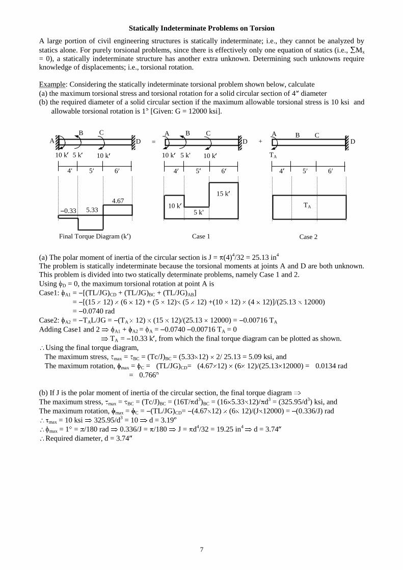
Statically Indeterminate Problems on Torsion
A large portion of civil engineering structures is statically indeterminate; i.e., they cannot be analyzed by
statics alone. For purely torsional problems, since there is effectively only one equation of statics (i.e., Mx
= 0), a statically indeterminate structure has another extra unknown. Determining such unknowns require
knowledge of displacements; i.e., torsional rotation.
Example: Considering the statically indeterminate torsional problem shown below, calculate
(a) the maximum torsional stress and torsional rotation for a solid circular section of 4 diameter
(b) the required diameter of a solid circular section if the maximum allowable torsional stress is 10 ksi and
allowable torsional rotation is 1 [Given: G = 12000 ksi].
(a) The polar moment of inertia of the circular section is J = (4)4/32 = 25.13 in
4
The problem is statically indeterminate because the torsional moments at joints A and D are both unknown.
This problem is divided into two statically determinate problems, namely Case 1 and 2.
Using D = 0, the maximum torsional rotation at point A is
Case1: A1 = [(TL/JG)CD + (TL/JG)BC + (TL/JG)AB]
= [(15 12) (6 12) + (5 12) (5 12) +(10 12) (4 12)]/(25.13 12000)
= 0.0740 rad
Case2: A2 = TAL/JG = (TA 12) (15 12)/(25.13 12000) = 0.00716 TA
Adding Case1 and 2 A1 + A2 = A = 0.0740 0.00716 TA = 0
TA = 10.33 k , from which the final torque diagram can be plotted as shown.
Using the final torque diagram,
The maximum stress, max = BC = (Tc/J)BC = (5.33 12) 2/ 25.13 = 5.09 ksi, and
The maximum rotation, max = C = (TL/JG)CD= (4.67 12) (6 12)/(25.13 12000) = 0.0134 rad
= 0.766
(b) If J is the polar moment of inertia of the circular section, the final torque diagram
The maximum stress, max = BC = (Tc/J)BC = (16T/ d3)BC = (16 5.33 12)/ d
3 = (325.95/d
3) ksi, and
The maximum rotation, max = C = (TL/JG)CD= (4.67 12) (6 12)/(J 12000) = (0.336/J) rad
max = 10 ksi 325.95/d3 = 10 d = 3.19
max = 1 = /180 rad 0.336/J = /180 J = d4/32 = 19.25 in
4 d = 3.74
Required diameter, d = 3.74
0.33
4.67
5.33 TA
5 k 10 k
6 5 4
C B
A
10 k 5 k 10 k
D
6 5 4
C B A
10 k 5 k 10 k
D
6 5 4
C B A
TA
D = +
Case 1 Case 2
15 k
Final Torque Diagram (k )
8
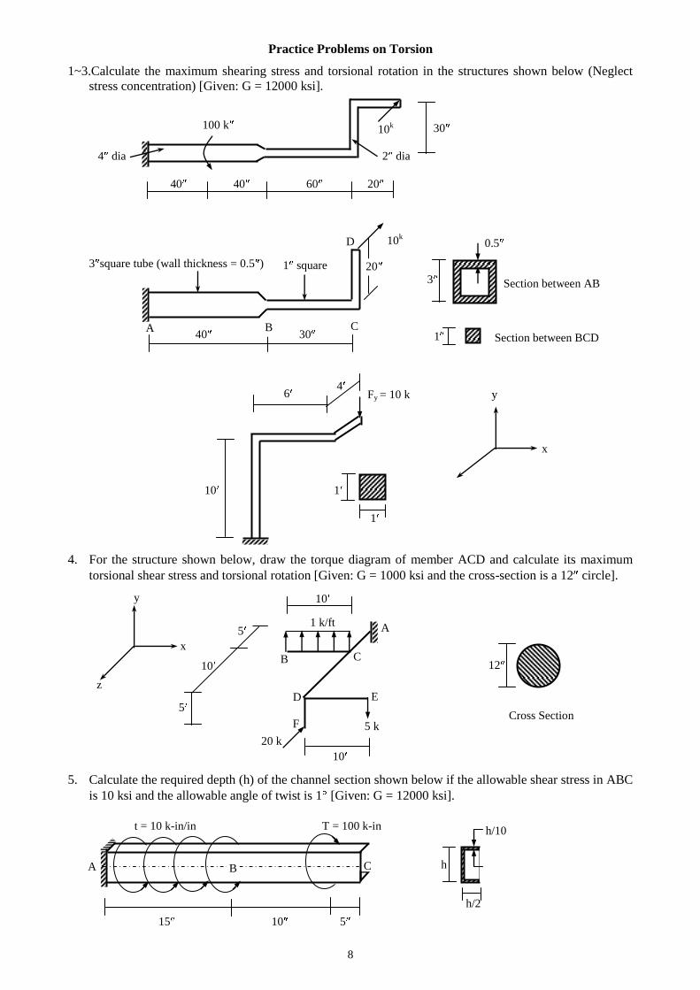
Practice Problems on Torsion
1~3.Calculate the maximum shearing stress and torsional rotation in the structures shown below (Neglect
stress concentration) [Given: G = 12000 ksi].
30
4 dia 2 dia
40 40 60 20
0.5
Section between AB
Section between BCD
Fy = 10 k y
x
10
1
1
4. For the structure shown below, draw the torque diagram of member ACD and calculate its maximum
torsional shear stress and torsional rotation [Given: G = 1000 ksi and the cross-section is a 12 circle].
5. Calculate the required depth (h) of the channel section shown below if the allowable shear stress in ABC
is 10 ksi and the allowable angle of twist is 1 [Given: G = 12000 ksi].
t = 10 k-in/in T = 100 k-in
15 10 5
D
A
1 square 3
1
3 square tube (wall thickness = 0.5 )
40 30 B C
20
10k
100 k 10k
6 4
5 k
20 k
E
C
F
A
5
10
5 1 k/ft
10
10
B
D
Cross Section
12
x
y
z
h/10
h
h/2
A C B
9
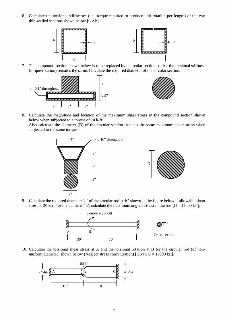
6. Calculate the torsional stiffnesses (i.e., torque required to produce unit rotation per length) of the two
thin-walled sections shown below [t b].
b
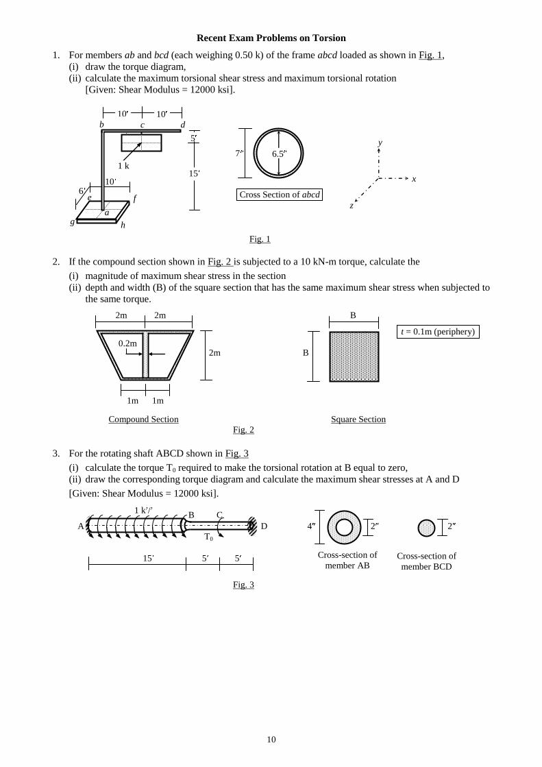
7. The compound section shown below is to be replaced by a circular section so that the torsional stiffness
(torque/rotation) remains the same. Calculate the required diameter of the circular section.
t = 0.1 throughout
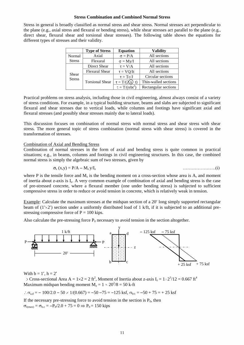
8. Calculate the magnitude and location of the maximum shear stress in the compound section shown
below when subjected to a torque of 10 k-ft.
Also calculate the diameter (D) of the circular section that has the same maximum shear stress when
subjected to the same torque.
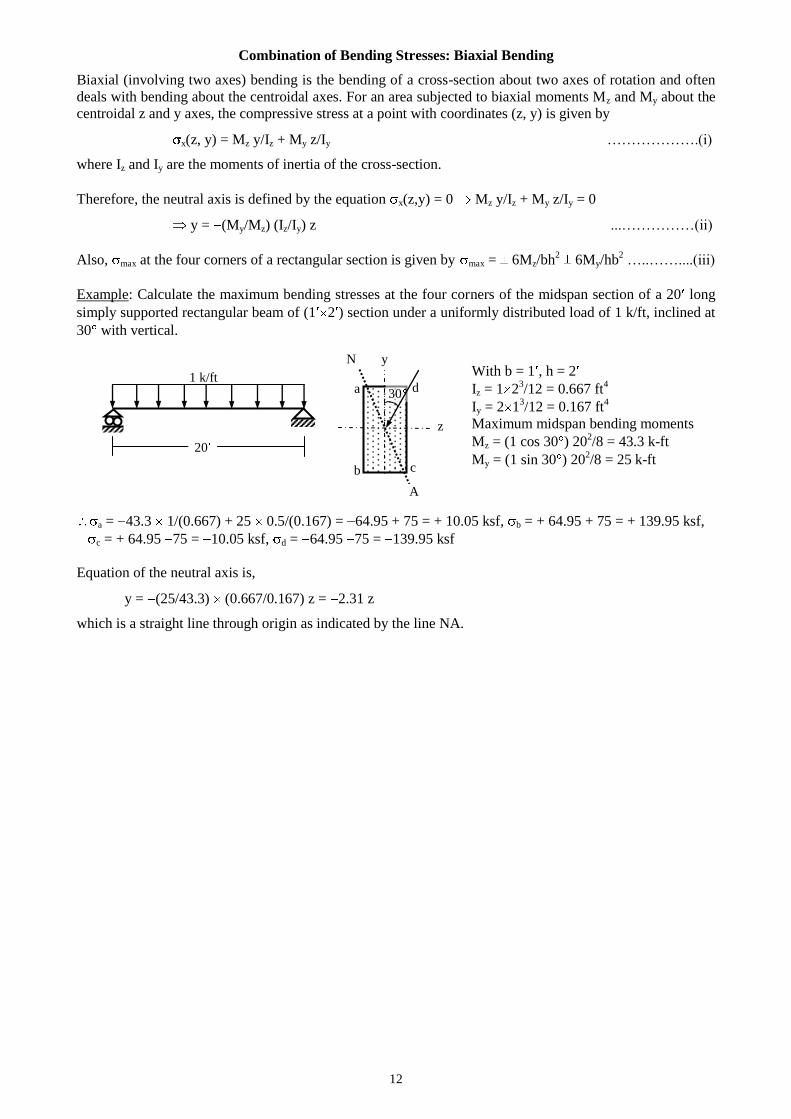
9. Calculate the required diameter ‘d’ of the circular rod ABC shown in the figure below if allowable shear
stress is 20 ksi. For the diameter ‘d’, calculate the maximum angle of twist in the rod [G = 12000 ksi].
30 70
10. Calculate the torsional shear stress at A and the torsional rotation at B for the circular rod (of non-
uniform diameter) shown below (Neglect stress concentration) [Given G = 12000 ksi].
2 dia 4 dia
2
2
2
2
4 t = 0.10 throughout
D
1 1 1
1
0.5
100 k
A C B
10 10
d
A B C
Torque = 10 k-ft
Cross-section
b
b t t
b
b
10
Recent Exam Problems on Torsion
1. For members ab and bcd (each weighing 0.50 k) of the frame abcd loaded as shown in Fig. 1,
(i) draw the torque diagram,
(ii) calculate the maximum torsional shear stress and maximum torsional rotation
[Given: Shear Modulus = 12000 ksi].
Fig. 1
2. If the compound section shown in Fig. 2 is subjected to a 10 kN-m torque, calculate the
(i) magnitude of maximum shear stress in the section
(ii) depth and width (B) of the square section that has the same maximum shear stress when subjected to
the same torque.
2m 2m B
2m B
1m 1m
Compound Section Square Section
Fig. 2
3. For the rotating shaft ABCD shown in Fig. 3
(i) calculate the torque T0 required to make the torsional rotation at B equal to zero,
(ii) draw the corresponding torque diagram and calculate the maximum shear stresses at A and D
[Given: Shear Modulus = 12000 ksi].
B C
A D 4 2 2
T0
15 5 5
Fig. 3
c b d
10 10
1 k
Cross Section of abcd
6.5 7
y
x
z
15
5
a
10 6
e f
g h
Cross-section of
member AB Cross-section of
member BCD
1 k /
t = 0.1m (periphery)
0.2m
11
Stress Combination and Combined Normal Stress
Stress in general is broadly classified as normal stress and shear stress. Normal stresses act perpendicular to
the plane (e.g., axial stress and flexural or bending stress), while shear stresses act parallel to the plane (e.g.,
direct shear, flexural shear and torsional shear stresses). The following table shows the equations for
different types of stresses and their validity.
Type of Stress Equation Validity
Normal
Stress
Axial = P/A All sections
Flexural = My/I All sections
Shear
Stress
Direct Shear = V/A All sections
Flexural Shear = VQ/It All sections
Torsional Shear
= Tc/J Circular sections
= T/(2 t) Thin-walled sections
= T/( bt2) Rectangular sections
Practical problems on stress analysis, including those in civil engineering, almost always consist of a variety
of stress conditions. For example, in a typical building structure, beams and slabs are subjected to significant
flexural and shear stresses due to vertical loads, while columns and footings have significant axial and
flexural stresses (and possibly shear stresses mainly due to lateral loads).
This discussion focuses on combination of normal stress with normal stress and shear stress with shear
stress. The more general topic of stress combination (normal stress with shear stress) is covered in the
transformation of stresses.
Combination of Axial and Bending Stress
Combination of normal stresses in the form of axial and bending stress is quite common in practical
situations; e.g., in beams, columns and footings in civil engineering structures. In this case, the combined
normal stress is simply the algebraic sum of two stresses, given by
z (x,y) = P/A Mz y/Iz ………………….(i)
where P is the tensile force and Mz is the bending moment on a cross-section whose area is A, and moment
of inertia about z-axis is Iz. A very common example of combination of axial and bending stress is the case
of pre-stressed concrete, where a flexural member (one under bending stress) is subjected to sufficient
compressive stress in order to reduce or avoid tension in concrete, which is relatively weak in tension.
Example: Calculate the maximum stresses at the midspan section of a 20 long simply supported rectangular
beam of (1 2 ) section under a uniformly distributed load of 1 k/ft, if it is subjected to an additional pre-
stressing compressive force of P = 100 kips.
Also calculate the pre-stressing force P0 necessary to avoid tension in the section altogether.
With b = 1 , h = 2
Cross-sectional Area A = 1 2 = 2 ft2, Moment of Inertia about z-axis Iz = 1 2
3/12 = 0.667 ft
4
Maximum midspan bending moment Mz = 1 202/8 = 50 k-ft
a,d = 100/2.0 50 1/(0.667) = 50 75 = 125 ksf, b/c = 50 + 75 = + 25 ksf
If the necessary pre-stressing force to avoid tension in the section is P0, then
t(max) = b.c = P0/2.0 + 75 = 0 P0 = 150 kips
A
c
d
b
a 1 k/ft
20
z
y
P P
125 ksf
+ 25 ksf
75 ksf
+ 75 ksf
12
Combination of Bending Stresses: Biaxial Bending
Biaxial (involving two axes) bending is the bending of a cross-section about two axes of rotation and often
deals with bending about the centroidal axes. For an area subjected to biaxial moments Mz and My about the
centroidal z and y axes, the compressive stress at a point with coordinates (z, y) is given by
x(z, y) = Mz y/Iz + My z/Iy ……………….(i)
where Iz and Iy are the moments of inertia of the cross-section.
Therefore, the neutral axis is defined by the equation x(z,y) = 0 Mz y/Iz + My z/Iy = 0
y = (My/Mz) (Iz/Iy) z ...……………(ii)
Also, max at the four corners of a rectangular section is given by max = 6Mz/bh2 6My/hb
2 …..……....(iii)
Example: Calculate the maximum bending stresses at the four corners of the midspan section of a 20 long
simply supported rectangular beam of (1 2 ) section under a uniformly distributed load of 1 k/ft, inclined at
30 with vertical.
a = 43.3 1/(0.667) + 25 0.5/(0.167) = 64.95 + 75 = + 10.05 ksf, b = + 64.95 + 75 = + 139.95 ksf,
c = + 64.95 75 = 10.05 ksf, d = 64.95 75 = 139.95 ksf
Equation of the neutral axis is,
y = (25/43.3) (0.667/0.167) z = 2.31 z
which is a straight line through origin as indicated by the line NA.
c
d
b
a 1 k/ft
20
z
y With b = 1 , h = 2
Iz = 1 23/12 = 0.667 ft
4
Iy = 2 13/12 = 0.167 ft
4
Maximum midspan bending moments
Mz = (1 cos 30 ) 202/8 = 43.3 k-ft
My = (1 sin 30 ) 202/8 = 25 k-ft
30
A
N
13
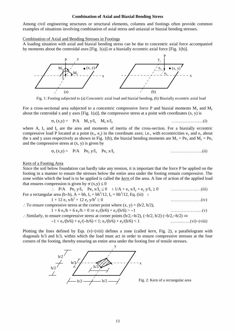
Combination of Axial and Biaxial Bending Stress
Among civil engineering structures or structural elements, columns and footings often provide common
examples of situations involving combination of axial stress and uniaxial or biaxial bending stresses.
Combination of Axial and Bending Stresses in Footings
A loading situation with axial and biaxial bending stress can be due to concentric axial force accompanied
by moments about the centroidal axes [Fig. 1(a)] or a biaxially eccentric axial force [Fig. 1(b)].
Fig. 1: Footing subjected to (a) Concentric axial load and biaxial bending, (b) Biaxially eccentric axial load
For a cross-sectional area subjected to a concentric compressive force P and biaxial moments Mx and My
about the centroidal x and y axes [Fig. 1(a)], the compressive stress at a point with coordinates (x, y) is
z (x,y) = P/A Mx y/Ix My x/Iy ………………….(i)
where A, Ix and Iy are the area and moments of inertia of the cross-section. For a biaxially eccentric
compressive load P located at a point (ex, ey) in the coordinate axes; i.e., with eccentricities ey and ex about
the x and y axes respectively as shown in Fig. 1(b), the biaxial bending moments are Mx = Pey and My = Pex
and the compressive stress at (x, y) is given by
z (x,y) = P/A Pey y/Ix Pex x/Iy ………………….(ii)
Kern of a Footing Area
Since the soil below foundation can hardly take any tension, it is important that the force P be applied on the
footing in a manner to ensure the stresses below the entire area under the footing remain compressive. The
zone within which the load is to be applied is called the kern of the area. A line of action of the applied load
that ensures compression is given by (x,y) 0
P/A Pey y/Ix Pex x/Iy 0 1/A + ex x/Iy + ey y/Ix 0 …………………(iii)
For a rectangular area (b h), A = bh, Ix = bh3/12, Iy = hb
3/12, Eq. (iii)
1 + 12 ex x/b2 + 12 ey y/h
2 0 …………………(iv)
To ensure compressive stress at the corner point where (x, y) = (b/2, h/2),
1 + 6 ex/b + 6 ey/h 0 ex/(b/6) + ey/(h/6) 1 ……………….…(v)
Similarly, to ensure compressive stress at corner points (b/2, h/2), ( b/2, h/2) ( b/2, h/2)
1 ex/(b/6) + ey/( h/6) 1; ex/(b/6) + ey/(h/6) 1 ……..……(vi)~(viii)
Plotting the lines defined by Eqs. (v)~(viii) defines a zone (called kern, Fig. 2), a parallelogram with
diagonals b/3 and h/3, within which the load must act in order to ensure compressive stresses at the four
corners of the footing, thereby ensuring an entire area under the footing free of tensile stresses.
x
y
x
y P
ey
ex Mx
My
(x, y) (x, y)
(a) (b)
x
y
h/3
b/2
h/2
h/2
b/2 Fig. 2: Kern of a rectangular area
b/3
P
14
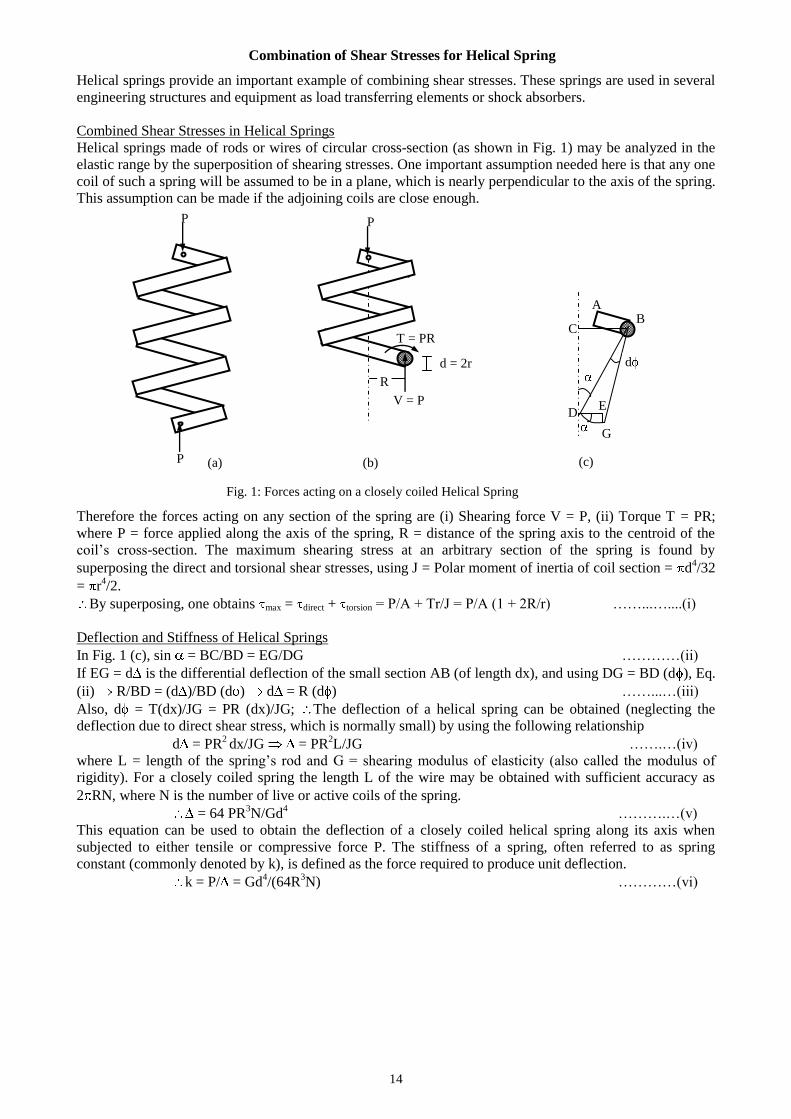
Combination of Shear Stresses for Helical Spring
Helical springs provide an important example of combining shear stresses. These springs are used in several
engineering structures and equipment as load transferring elements or shock absorbers.
Combined Shear Stresses in Helical Springs
Helical springs made of rods or wires of circular cross-section (as shown in Fig. 1) may be analyzed in the
elastic range by the superposition of shearing stresses. One important assumption needed here is that any one
coil of such a spring will be assumed to be in a plane, which is nearly perpendicular to the axis of the spring.
This assumption can be made if the adjoining coils are close enough.
Therefore the forces acting on any section of the spring are (i) Shearing force V = P, (ii) Torque T = PR;
where P = force applied along the axis of the spring, R = distance of the spring axis to the centroid of the
coil’s cross-section. The maximum shearing stress at an arbitrary section of the spring is found by
superposing the direct and torsional shear stresses, using J = Polar moment of inertia of coil section = d4/32
= r4/2.
By superposing, one obtains max = direct + torsion = P/A + Tr/J = P/A (1 + 2R/r) ……...…....(i)
Deflection and Stiffness of Helical Springs
In Fig. 1 (c), sin = BC/BD = EG/DG …………(ii)
If EG = d is the differential deflection of the small section AB (of length dx), and using DG = BD (d ), Eq.
(ii) R/BD = (d )/BD (d ) d = R (d ) ……...…(iii)
Also, d = T(dx)/JG = PR (dx)/JG; The deflection of a helical spring can be obtained (neglecting the
deflection due to direct shear stress, which is normally small) by using the following relationship
d = PR2 dx/JG = PR
2L/JG …….…(iv)
where L = length of the spring’s rod and G = shearing modulus of elasticity (also called the modulus of
rigidity). For a closely coiled spring the length L of the wire may be obtained with sufficient accuracy as
2 RN, where N is the number of live or active coils of the spring.
= 64 PR3N/Gd
4 ……….…(v)
This equation can be used to obtain the deflection of a closely coiled helical spring along its axis when
subjected to either tensile or compressive force P. The stiffness of a spring, often referred to as spring
constant (commonly denoted by k), is defined as the force required to produce unit deflection.
k = P/ = Gd4/(64R
3N) …………(vi)
E D
C
A B
P
P P
V = P
T = PR
d = 2r
R
Fig. 1: Forces acting on a closely coiled Helical Spring
G
d
(a) (b) (c)
15
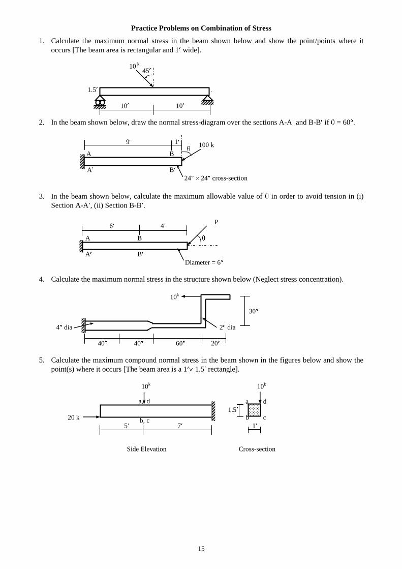
Practice Problems on Combination of Stress
1. Calculate the maximum normal stress in the beam shown below and show the point/points where it
occurs [The beam area is rectangular and 1 wide].
1.5
10 10
2. In the beam shown below, draw the normal stress-diagram over the sections A-A and B-B if = 60 .
A B
A B
24 24 cross-section
3. In the beam shown below, calculate the maximum allowable value of in order to avoid tension in (i)
Section A-A , (ii) Section B-B .
P
A B
A B
Diameter = 6
4. Calculate the maximum normal stress in the structure shown below (Neglect stress concentration).
30
4 dia 2 dia
40 40 60 20
5. Calculate the maximum compound normal stress in the beam shown in the figures below and show the
point(s) where it occurs [The beam area is a 1 1.5 rectangle].
a d
1.5
20 k b c
5 7 1
Side Elevation Cross-section
45
10k
10 k
b, c
a, d
9 1 100 k
6 4
10k 10
k
16
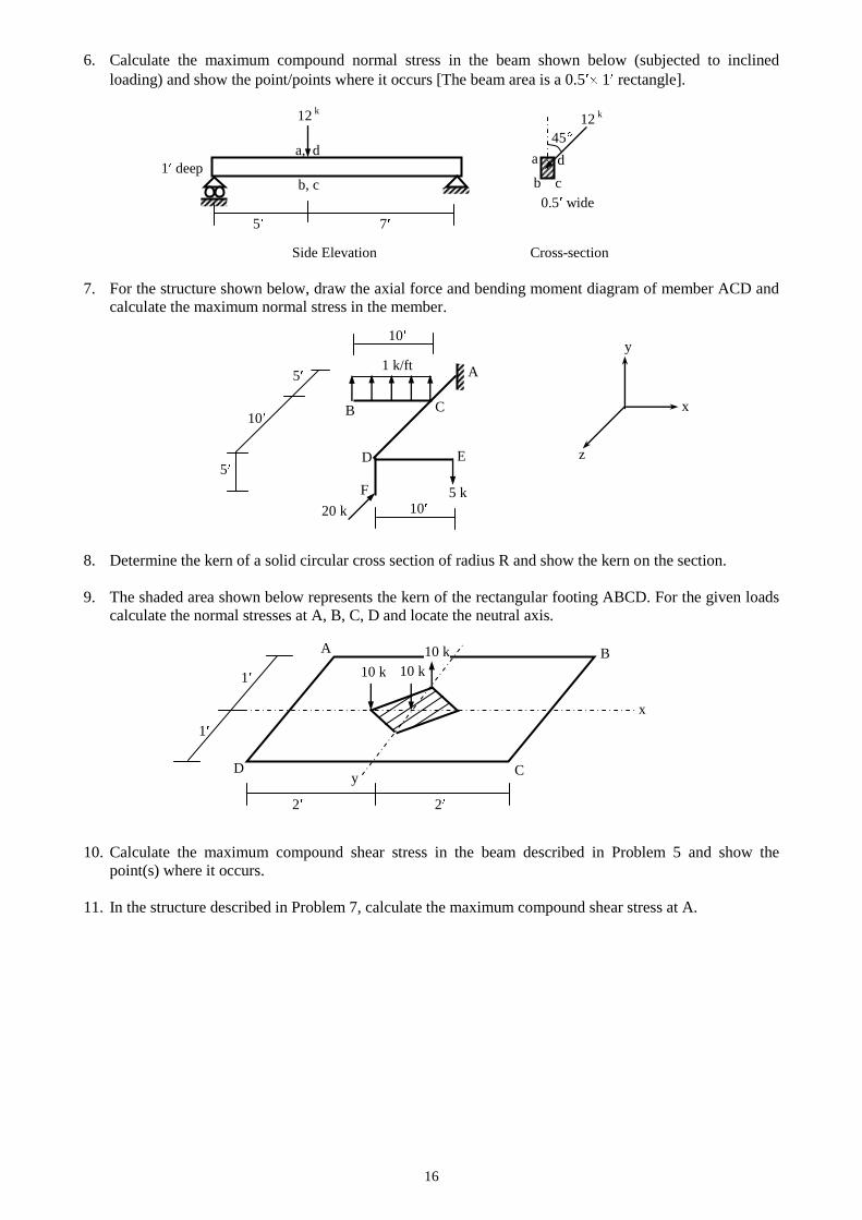
6. Calculate the maximum compound normal stress in the beam shown below (subjected to inclined
loading) and show the point/points where it occurs [The beam area is a 0.5 1 rectangle].
a, d
1 deep
b, c
0.5 wide
Side Elevation Cross-section
7. For the structure shown below, draw the axial force and bending moment diagram of member ACD and
calculate the maximum normal stress in the member.
8. Determine the kern of a solid circular cross section of radius R and show the kern on the section.
9. The shaded area shown below represents the kern of the rectangular footing ABCD. For the given loads
calculate the normal stresses at A, B, C, D and locate the neutral axis.
10. Calculate the maximum compound shear stress in the beam described in Problem 5 and show the
point(s) where it occurs.
11. In the structure described in Problem 7, calculate the maximum compound shear stress at A.
12 k
45
5 k
20 k
E
C
F
A
5
10
5 1 k/ft
10
10
B
D
x
y
z
x
y
A B
C D
10 k
10 k
2 2
1
1 10 k
d a
b c
5 7
12 k
17
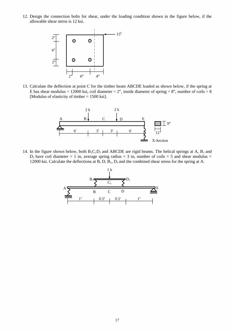
12. Design the connection bolts for shear, under the loading condition shown in the figure below, if the
allowable shear stress is 12 ksi.
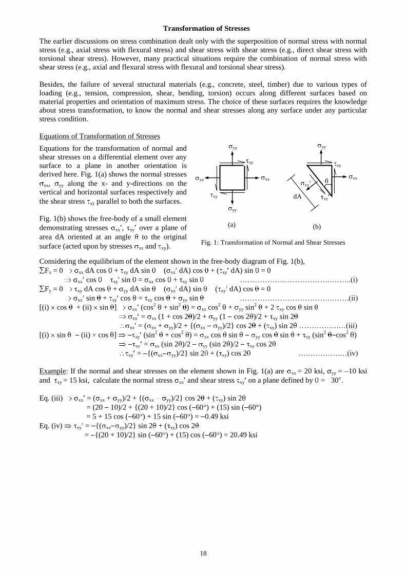
13. Calculate the deflection at point C for the timber beam ABCDE loaded as shown below, if the spring at
E has shear modulus = 12000 ksi, coil diameter = 2 , inside diameter of spring = 8 , number of coils = 8
[Modulus of elasticity of timber = 1500 ksi].
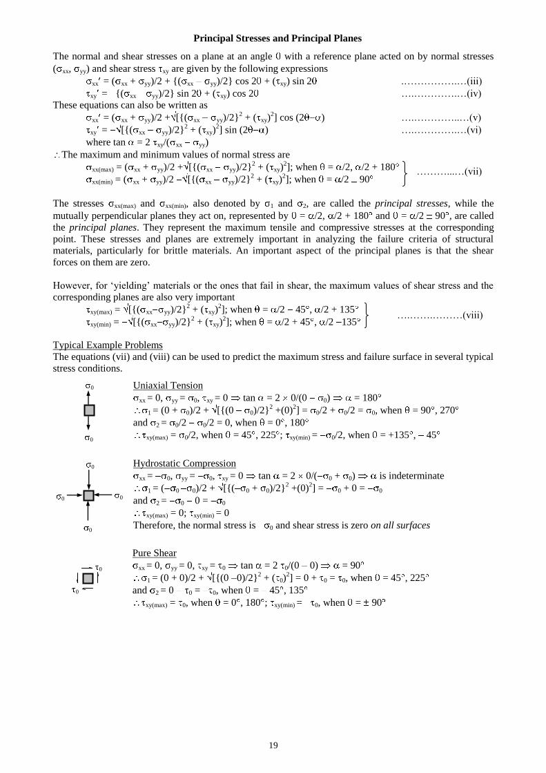
14. In the figure shown below, both B1C1D1 and ABCDE are rigid beams. The helical springs at A, B1 and
D1 have coil diameter = 1 in, average spring radius = 3 in, number of coils = 5 and shear modulus =
12000 ksi. Calculate the deflections at B, D, B1, D1 and the combined shear stress for the spring at A.
2 6 4
15k
6
2
2
1 0.5 1 0.5
1 k
A B D
E C
B1
C1
D1
6 3 3 6
2 k 2 k
A B C D
12
9
X-Section
E
18
Transformation of Stresses
The earlier discussions on stress combination dealt only with the superposition of normal stress with normal
stress (e.g., axial stress with flexural stress) and shear stress with shear stress (e.g., direct shear stress with
torsional shear stress). However, many practical situations require the combination of normal stress with
shear stress (e.g., axial and flexural stress with flexural and torsional shear stress).
Besides, the failure of several structural materials (e.g., concrete, steel, timber) due to various types of
loading (e.g., tension, compression, shear, bending, torsion) occurs along different surfaces based on
material properties and orientation of maximum stress. The choice of these surfaces requires the knowledge
about stress transformation, to know the normal and shear stresses along any surface under any particular
stress condition.
Equations of Transformation of Stresses
Considering the equilibrium of the element shown in the free-body diagram of Fig. 1(b),
Fx = 0 xx dA cos + xy dA sin ( xx dA) cos + ( xy dA) sin = 0
xx cos xy sin = xx cos + xy sin ……………………………….……..(i)
Fy = 0 xy dA cos + yy dA sin ( xx dA) sin ( xy dA) cos = 0
xx sin + xy cos = xy cos + yy sin ……………………………….…….(ii)
[(i) cos + (ii) sin ] xx (cos2 + sin
2 ) = xx cos
2 + yy sin
2 + 2 xy cos sin
xx = xx (1 + cos 2 )/2 + yy (1 cos 2 )/2 + xy sin 2
xx = ( xx + yy)/2 + {( xx yy)/2} cos 2 + ( xy) sin 2 …………….…(iii)
[(i) sin (ii) cos ] xy (sin2 + cos
2 ) = xx cos sin yy cos sin + xy (sin
2 cos
2 )
xy = xx (sin 2 )/2 yy (sin 2 )/2 xy cos 2
xy = {( xx yy)/2} sin 2 + ( xy) cos 2 ….………….…(iv)
Example: If the normal and shear stresses on the element shown in Fig. 1(a) are xx = 20 ksi, yy = 10 ksi
and xy = 15 ksi, calculate the normal stress xx and shear stress xy on a plane defined by = 30 .
Eq. (iii) xx = ( xx + yy)/2 + {( xx yy)/2} cos 2 + ( xy) sin 2
= (20 10)/2 + {(20 + 10)/2} cos ( 60 ) + (15) sin ( 60 )
= 5 + 15 cos ( 60 ) + 15 sin ( 60 ) = 0.49 ksi
Eq. (iv) xy = {( xx yy)/2} sin 2 + ( xy) cos 2
= {(20 + 10)/2} sin ( 60 ) + (15) cos ( 60 ) = 20.49 ksi
yy
yy
xx xx
xy
xy
Equations for the transformation of normal and
shear stresses on a differential element over any
surface to a plane in another orientation is
derived here. Fig. 1(a) shows the normal stresses
xx, yy along the x- and y-directions on the
vertical and horizontal surfaces respectively and
the shear stress xy parallel to both the surfaces.
Fig. 1(b) shows the free-body of a small element
demonstrating stresses xx , xy over a plane of
area dA oriented at an angle to the original
surface (acted upon by stresses xx and xy).
Fig. 1: Transformation of Normal and Shear Stresses
yy
xx
xy
xx
xy
(a) (b)
dA
19
Principal Stresses and Principal Planes
The normal and shear stresses on a plane at an angle with a reference plane acted on by normal stresses
( xx, yy) and shear stress xy are given by the following expressions
xx = ( xx + yy)/2 + {( xx yy)/2} cos 2 + ( xy) sin 2 .…………….…(iii)
xy = {( xx yy)/2} sin 2 + ( xy) cos 2 ….………….…(iv)
These equations can also be written as
xx = ( xx + yy)/2 + [{( xx yy)/2}2 + ( xy)
2] cos (2 ) ….…………..…(v)
xy = [{( xx yy)/2}2 + ( xy)
2] sin (2 ) ….………….…(vi)
where tan = 2 xy/( xx yy)
The maximum and minimum values of normal stress are
xx(max) = ( xx + yy)/2 + [{( xx yy)/2}2 + ( xy)
2]; when = /2, /2 + 180
xx(min) = ( xx + yy)/2 [{( xx yy)/2}2 + ( xy)
2]; when = /2 90
The stresses xx(max) and xx(min), also denoted by 1 and 2, are called the principal stresses, while the
mutually perpendicular planes they act on, represented by = /2, /2 + 180 and = /2 90 , are called
the principal planes. They represent the maximum tensile and compressive stresses at the corresponding
point. These stresses and planes are extremely important in analyzing the failure criteria of structural
materials, particularly for brittle materials. An important aspect of the principal planes is that the shear
forces on them are zero.
However, for ‘yielding’ materials or the ones that fail in shear, the maximum values of shear stress and the
corresponding planes are also very important
xy(max) = [{( xx yy)/2}2 + ( xy)
2]; when = /2 45 , /2 + 135
xy(min) = [{( xx yy)/2}2 + ( xy)
2]; when = /2 + 45 , /2 135
Typical Example Problems
The equations (vii) and (viii) can be used to predict the maximum stress and failure surface in several typical
stress conditions.
………...…(vii)
….…….………(viii)
Uniaxial Tension
xx = 0, yy = 0, xy = 0 tan = 2 0/(0 0) = 180
1 = (0 + 0)/2 + [{(0 0)/2}2 +(0)
2] = 0/2 + 0/2 = 0, when = 90 , 270
and 2 = 0/2 0/2 = 0, when = 0 , 180
xy(max) = 0/2, when = 45 , 225 ; xy(min) = 0/2, when = +135 , 45
Hydrostatic Compression
xx = 0, yy = 0, xy = 0 tan = 2 0/( 0 + 0) is indeterminate
1 = ( 0 0)/2 + [{( 0 + 0)/2}2 +(0)
2] = 0 + 0 = 0
and 2 = 0 0 = 0
xy(max) = 0; xy(min) = 0
Therefore, the normal stress is 0 and shear stress is zero on all surfaces
Pure Shear
xx = 0, yy = 0, xy = 0 tan = 2 0/(0 0) = 90
1 = (0 + 0)/2 + [{(0 0)/2}2 + ( 0)
2] = 0 + 0 = 0, when = 45 , 225
and 2 = 0 0 = 0, when = 45 , 135
xy(max) = 0, when = 0 , 180 ; xy(min) = 0, when = 90
0
0
0 0
0
0
0
0
20
Mohr’s Circle
The equations for the normal and shear stresses on a plane at angle with a reference plane acted on by
normal stresses ( xx, yy) and shear stress xy have been derived to be
xx = ( xx + yy)/2 + [{( xx yy)/2}2 + ( xy)
2] cos (2 ) ….…………..…(v)
xy = [{( xx yy)/2}2 + ( xy)
2] sin (2 ) ….………….…(vi)
where tan = 2 xy/( xx yy)
These equations can be re-adjusted to the following form
{ xx ( xx + yy)/2}2 + ( xy 0)
2 = {( xx yy)/2}
2 + ( xy)
2 ….………….…(ix)
Eq. (ix), when plotted with xx in x-axis and xy in y-axis, takes the form (X a)2 + (Y 0)
2 = R
2, which is the
equation of a circle with center(a, 0) = [( xx + yy)/2, 0] and radius R = [{( xx yy)/2}2 + ( xy)
2]. This circle
is called Mohr’s Circle, after Otto Mohr of Germany, who first suggested it in 1895.
Example: For an infinitesimal element, xx = 30 ksi, yy = 10 ksi, and xy = 15 ksi. In Mohr’s circle of
stress, show the normal and shear stresses acting on a plane defined by = 15 .
The coordinates of the center of the circle = [( xx + yy)/2, 0] = [( 30 + 10)/2, 0] = ( 10, 0) and
radius R = [{( xx yy)/2}2 + ( xy)
2] = [{( 30 10)/2}
2 + ( 15)
2] = 25
( 10, 25)
( 19.8, 23.0)
(0, 0)
( 10, 0)
( xx , xy )
Fig. 1 shows a Mohr’s Circle with some of its more
important features. Among them, the coordinates of
the center of the circle = (a, 0) = [( xx + yy)/2, 0] and
radius R = [{( xx yy)/2}2
+ ( xy)2] have already
been mentioned before.
However, the figure also shows that the principal
stresses are 1 = a + R, 2 = a R,
while the maximum and minimum shear stresses are
max = R and min = R.
Since the center of the circle is at the midpoint of all
radial lines, ( 1 + 2)/2 = ( xx + yy)/2 = a
Also from figure, tan = ( xy 0)/( xx ( xx + yy)/2) =
2 xy /( xx yy) = tan ; = .
It can also be proved that if the slope of AB with
vertical is , the coordinates of B = ( xx , xy ).
Fig. 1: Mohr’s Circle
xx
xy
( 1, 0) ( 2, 0)
R
R
R (a, 0)
(a, min)
( xx, xy)
( xx , xy )
=
2
O
A
B
The principal stresses are
1 = a + R = 10 + 25 = 15 ksi,
and 2 = 10 25 = 35 ksi.
max = R = 25 ksi, and min = 25 ksi.
tan = 2 xy/( xx yy) = ( 30)/( 40) = = 216.9
The coordinates of B = ( 19.8, 23.0) = ( xx , xy )
xx = 19.8 ksi, xy = 23.0 ksi
( 10, 25)
( 30, 15)
( 35, 0) (15, 0)
A
B
216.9
19.8
23.0
(a, max)
15
21
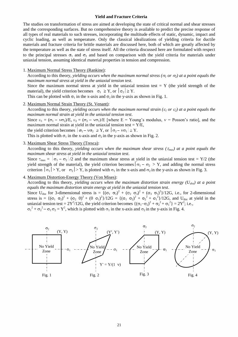
Yield and Fracture Criteria
The studies on transformation of stress are aimed at developing the state of critical normal and shear stresses
and the corresponding surfaces. But no comprehensive theory is available to predict the precise response of
all types of real materials to such stresses, incorporating the multitude effects of static, dynamic, impact and
cyclic loading, as well as temperature. Only the classical idealizations of yielding criteria for ductile
materials and fracture criteria for brittle materials are discussed here, both of which are greatly affected by
the temperature as well as the state of stress itself. All the criteria discussed here are formulated with respect
to the principal stresses 1 and 2 and based on comparison with the yield criteria for materials under
uniaxial tension, assuming identical material properties in tension and compression.
1. Maximum Normal Stress Theory (Rankine):
According to this theory, yielding occurs when the maximum normal stress ( 1 or 2) at a point equals the
maximum normal stress at yield in the uniaxial tension test.
Since the maximum normal stress at yield in the uniaxial tension test = Y (the yield strength of the
material), the yield criterion becomes 1 Y, or 2 Y.
This can be plotted with 1 in the x-axis and 2 in the y-axis as shown in Fig. 1.
2. Maximum Normal Strain Theory (St. Venant):
According to this theory, yielding occurs when the maximum normal strain ( 1 or 2) at a point equals the
maximum normal strain at yield in the uniaxial tension test.
Since 1 = ( 1 2)/E, 2 = ( 2 1)/E [where E = Young’s modulus, = Posson’s ratio], and the
maximum normal strain at yield in the uniaxial tension test = Y/E,
the yield criterion becomes 1 2 Y, or 2 1 Y.
This is plotted with 1 in the x-axis and 2 in the y-axis as shown in Fig. 2.
3. Maximum Shear Stress Theory (Tresca):
According to this theory, yielding occurs when the maximum shear stress ( max) at a point equals the
maximum shear stress at yield in the uniaxial tension test.
Since max = 1 2 /2 and the maximum shear stress at yield in the uniaxial tension test = Y/2 (the
yield strength of the material), the yield criterion becomes 1 2 Y, and adding the normal stress
criterion 1 Y, or 2 Y, is plotted with 1 in the x-axis and 2 in the y-axis as shown in Fig. 3.
4. Maximum Distortion-Energy Theory (Von Mises):
According to this theory, yielding occurs when the maximum distortion strain energy (Udist) at a point
equals the maximum distortion strain energy at yield in the uniaxial tension test.
Since Udist for 3-dimensional stress is = {( 1 2)2 + ( 2 3)
2 + ( 3 1)
2}/12G, i.e., for 2-dimensional
stress is = {( 1 2)2 + ( 2 0)
2 + (0 1)
2}/12G = {( 1 2)
2 + 2
2 + 1
2}/12G, and Udist at yield in the
uniaxial tension test = 2Y2/12G, the yield criterion becomes {( 1 2)
2 + 2
2 + 1
2} = 2Y
2; i.e.,
12 + 2
2 1 2 = Y
2, which is plotted with 1 in the x-axis and 2 in the y-axis in Fig. 4.
(Y, Y) (Y, Y) (Y , Y ) (Y, Y)
1 1 1 1
2 2 2 2
Fig. 1 Fig. 2 Fig. 3 Fig. 4
No Yield
Zone No Yield
Zone
No Yield
Zone
No Yield
Zone
Y = Y/(1 )
22
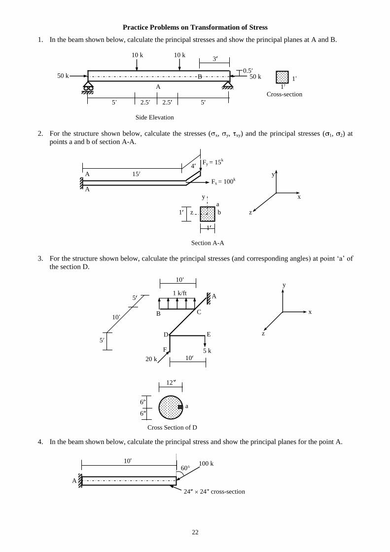
Practice Problems on Transformation of Stress
1. In the beam shown below, calculate the principal stresses and show the principal planes at A and B.
10 k 10 k
0.5
1
A 1
Cross-section
5 2.5 2.5 5
Side Elevation
2. For the structure shown below, calculate the stresses ( x, y, xy) and the principal stresses ( 1, 2) at
points a and b of section A-A.
4
A 15 y
Fx = 100k
A
y
x
a
1 z b
z
1
Section A-A
3. For the structure shown below, calculate the principal stresses (and corresponding angles) at point ‘a’ of
the section D.
4. In the beam shown below, calculate the principal stress and show the principal planes for the point A.
Cross Section of D
6
12
6
a
5 k
20 k
E
C
F
A
5
10
5 1 k/ft
10
10
B
D
x
y
z
10 100 k 60
A
Fy = 15k
3
50 k 50 k B
24 24 cross-section
23
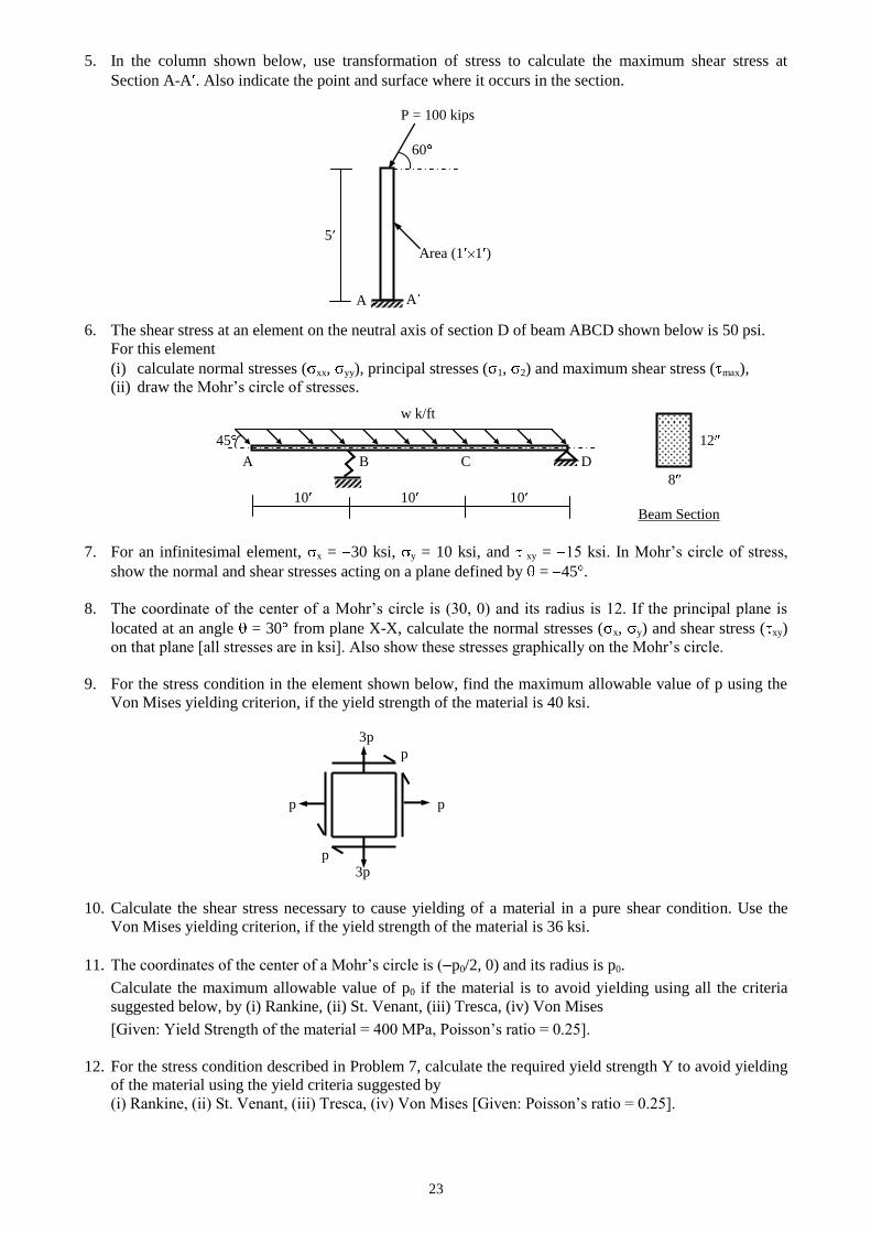
5. In the column shown below, use transformation of stress to calculate the maximum shear stress at
Section A-A . Also indicate the point and surface where it occurs in the section.
P = 100 kips
60
5
Area (1 1 )
6. The shear stress at an element on the neutral axis of section D of beam ABCD shown below is 50 psi.
For this element
(i) calculate normal stresses ( xx, yy), principal stresses ( 1, 2) and maximum shear stress ( max),
(ii) draw the Mohr’s circle of stresses.
w k/ft
45 12
A B C D
8
10 10 10
Beam Section
7. For an infinitesimal element, x = 30 ksi, y = 10 ksi, and xy = 15 ksi. In Mohr’s circle of stress,
show the normal and shear stresses acting on a plane defined by = 45 .
8. The coordinate of the center of a Mohr’s circle is (30, 0) and its radius is 12. If the principal plane is
located at an angle = 30 from plane X-X, calculate the normal stresses ( x, y) and shear stress ( xy)
on that plane [all stresses are in ksi]. Also show these stresses graphically on the Mohr’s circle.
9. For the stress condition in the element shown below, find the maximum allowable value of p using the
Von Mises yielding criterion, if the yield strength of the material is 40 ksi.
3p
p
p p
p
3p
10. Calculate the shear stress necessary to cause yielding of a material in a pure shear condition. Use the
Von Mises yielding criterion, if the yield strength of the material is 36 ksi.
11. The coordinates of the center of a Mohr’s circle is ( p0/2, 0) and its radius is p0.
Calculate the maximum allowable value of p0 if the material is to avoid yielding using all the criteria
suggested below, by (i) Rankine, (ii) St. Venant, (iii) Tresca, (iv) Von Mises
[Given: Yield Strength of the material = 400 MPa, Poisson’s ratio = 0.25].
12. For the stress condition described in Problem 7, calculate the required yield strength Y to avoid yielding
of the material using the yield criteria suggested by
(i) Rankine, (ii) St. Venant, (iii) Tresca, (iv) Von Mises [Given: Poisson’s ratio = 0.25].
A A
24
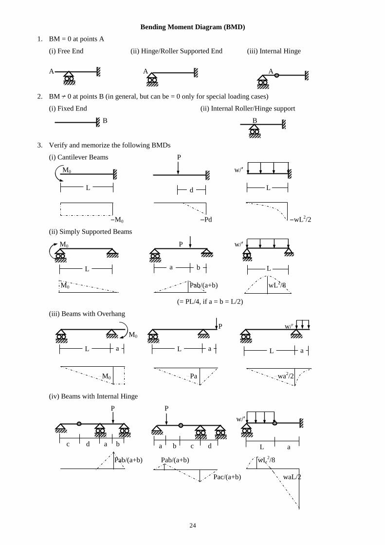
Bending Moment Diagram (BMD)
1. BM = 0 at points A
(i) Free End (ii) Hinge/Roller Supported End (iii) Internal Hinge
A A A
2. BM 0 at points B (in general, but can be = 0 only for special loading cases)
(i) Fixed End (ii) Internal Roller/Hinge support
B B
3. Verify and memorize the following BMDs
(i) Cantilever Beams P
M0 w/
M0 Pd wL2/2
(ii) Simply Supported Beams
M0 P w/
M0 Pab/(a+b) wL2/8
(= PL/4, if a = b = L/2)
(iii) Beams with Overhang
P w/
M0
M0 Pa wa2/2
(iv) Beams with Internal Hinge
P P
w/
Pab/(a+b) Pab/(a+b) wL2/8
Pac/(a+b) waL/2
L d L
L a b L
a L a L a L
c d a b a b c d L a
25
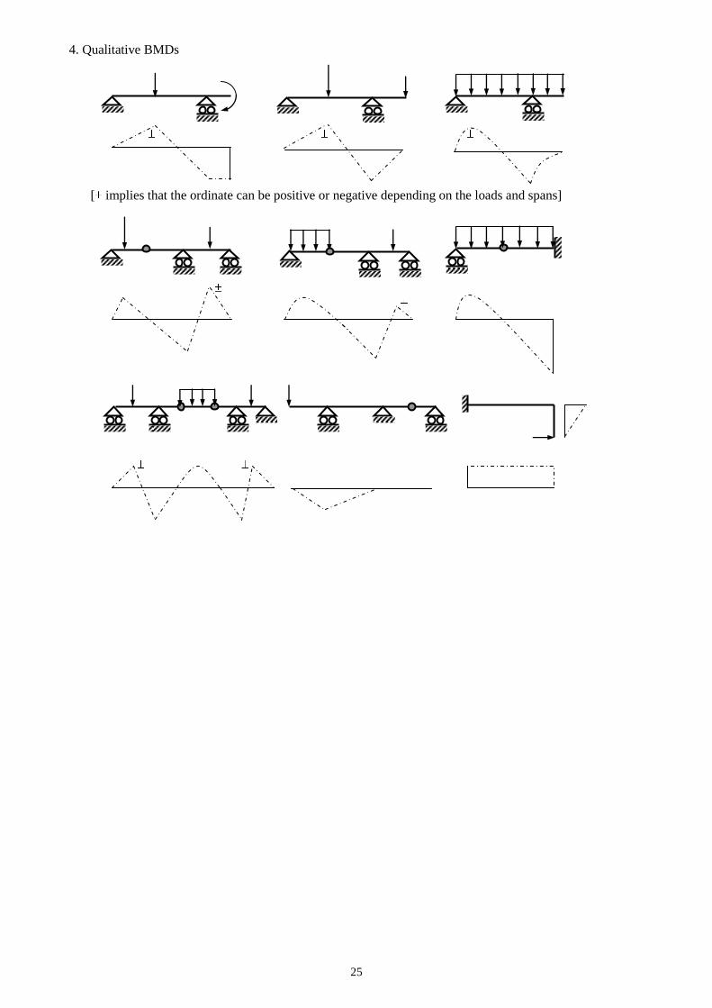
4. Qualitative BMDs
[ implies that the ordinate can be positive or negative depending on the loads and spans]
26
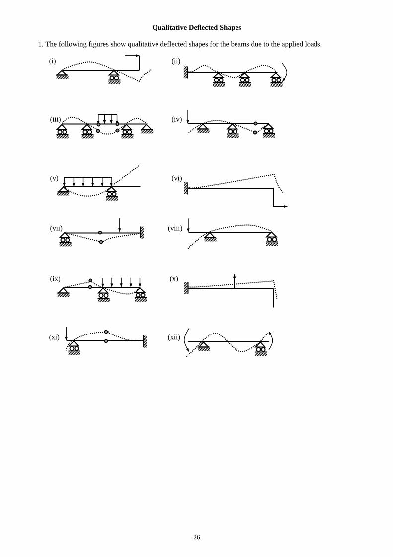
Qualitative Deflected Shapes
1. The following figures show qualitative deflected shapes for the beams due to the applied loads.
(i) (ii)
(iii) (iv)
(v) (vi)
(vii) (viii)
(ix) (x)
(xi) (xii)
27
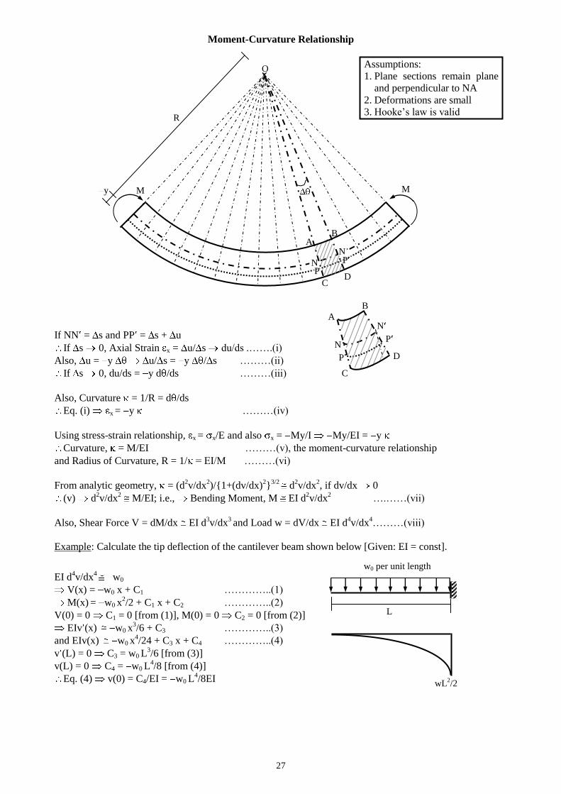
Moment-Curvature Relationship
If NN = s and PP = s + u
If s 0, Axial Strain x = u/ s du/ds .…….(i)
Also, u = y u/ s = y / s ………(ii)
If s 0, du/ds = y d /ds ………(iii)
Also, Curvature = 1/R = d /ds
Eq. (i) x = y ………(iv)
Using stress-strain relationship, x = x/E and also x = My/I My/EI = y
Curvature, = M/EI ………(v), the moment-curvature relationship
and Radius of Curvature, R = 1/ = EI/M ………(vi)
From analytic geometry, = (d2v/dx
2)/{1+(dv/dx)
2}
3/2 d
2v/dx
2, if dv/dx 0
(v) d2v/dx
2 M/EI; i.e., Bending Moment, M EI d
2v/dx
2 ….……(vii)
Also, Shear Force V = dM/dx EI d3v/dx
3 and Load w = dV/dx EI d
4v/dx
4………(viii)
Example: Calculate the tip deflection of the cantilever beam shown below [Given: EI = const].
EI d4v/dx
4 w0
V(x) = w0 x + C1 …………..(1)
M(x) = w0 x
2/2 + C1 x + C2 …………..(2)
V(0) = 0 C1 = 0 [from (1)], M(0) = 0 C2 = 0 [from (2)]
EIv (x)
w0 x3/6 + C3 …………..(3)
and EIv(x)
w0 x4/24 + C3 x + C4 …………..(4)
v (L) = 0 C3 = w0 L3/6 [from (3)]
v(L) = 0 C4 = w0 L4/8 [from (4)]
Eq. (4) v(0) = C4/EI = w0 L4/8EI
O
D C
A B
R
N
N
D
C
A
B
P
P
y
w0 per unit length
L
wL2/2
M M
Assumptions:
1. Plane sections remain plane
and perpendicular to NA
2. Deformations are small
3. Hooke’s law is valid
P N
N P
28
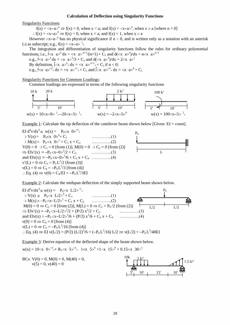
Calculation of Deflection using Singularity Functions
Singularity Functions:
f(x) = x an f(x) = 0, when x a; and f(x) = x a
n, when x a [where n 0]
f(x) = x a0 f(x) = 0, when x a; and f(x) = 1, when x a
However x an has no physical significance if n 0, and is written only as a notation with an asterisk
(*) as subscript; e.g., f(x) = x a1
*
The integration and differentiation of singularity functions follow the rules for ordinary polynomial
functions; i.e., x an dx = x a
n+1/(n+1)
+ C1 and d( x a
n)/dx = n x a
n 1
e.g., x a2 dx = x a
3/3 + C1 and d( x a
2)/dx = 2 x a
1
By definition, x an* dx = x a
n+1* + C1 if n 0;
e.g., x a2* dx = x a
1* + C1 and x a
1* dx = x a
0 + C1
Singularity Functions for Common Loadings:
Common loadings are expressed in terms of the following singularity functions
w(x) = 10 x 01* 20 x 5
1* w(x) = 2 x 5
0 w(x) = 100 x 5
2*
Example 1: Calculate the tip deflection of the cantilever beam shown below [Given: EI = const].
EI d4v/dx
4 w(x) = P0 x 0
1*
V(x) = P0 x 0
0+ C1 …………..(1)
M(x) = P0 x 0
1 + C1 x + C2 …………..(2)
V(0) = 0 C1 = 0 [from (1)], M(0) = 0 C2 = 0 [from (2)]
EIv (x)
P0 x 02/2 + C3 …………..(3)
and EIv(x)
P0 x 03/6 + C3 x + C4 …………..(4)
v (L) = 0 C3 = P0 L2/2 [from (3)]
v(L) = 0 C4 = P0 L3/3 [from (4)]
Eq. (4) v(0) = C4/EI = P0 L3/3EI
Example 2: Calculate the midspan deflection of the simply supported beam shown below.
EI d4v/dx
4 w(x) = P0 x L/2
1*
V(x)
P0 x L/20 + C1 …………..(1)
M(x)
P0 x L/21 + C1 x + C2 …………..(2)
M(0) = 0 C2 = 0 [from (2)], M(L) = 0 C1 = P0 /2 [from (2)]
EIv (x) P0 x L/22/2 + (P/2) x
2/2 + C3 …………..(3)
and EIv(x) P0 x L/23/6 + (P/2) x
3/6 + C3 x + C4 …………..(4)
v(0) = 0 C4 = 0 [from (4)]
v(L) = 0 C3 = P0 L2/16 [from (4)]
Eq. (4) EI v(L/2) = (P/2) (L/2)3/6 + ( P0 L
2/16) L/2 v(L/2) = P0 L
3/48EI
Example 3: Derive equation of the deflected shape of the beam shown below.
w(x) = 10 x 01
*+ R1 x 51
* 1 x 50 +1 x 15
0 + 0.15 x 30
1
BCs: V(0) = 0, M(0) = 0, M(40) = 0, v(5) = 0, v(40) = 0
10 k 20 k
5 10 5 10
2 k/
5 10
100 k
P0
L
L/2 L/2
5 10 10 15
10k 1 k/ 1.5 k/
P0
29
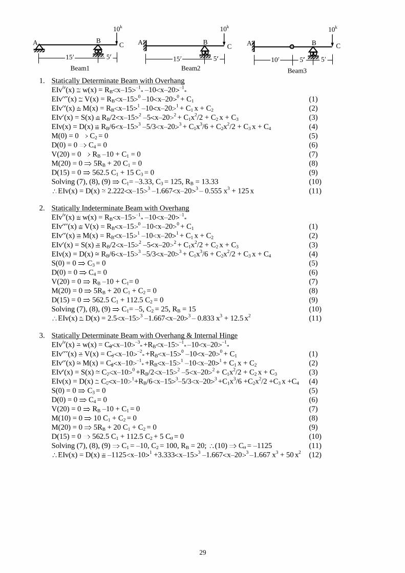
1. Statically Determinate Beam with Overhang
EIviv(x) w(x) = RB x–15
–1* –10 x–20
–1*
EIv (x) V(x) = RB x–150 –10 x–20
0 + C1 (1)
EIv (x) M(x) = RB x–151 –10 x–20
1 + C1 x + C2 (2)
EIv (x) = S(x) RB/2 x–152 –5 x–20
2 + C1x
2/2 + C2 x + C3 (3)
EIv(x) = D(x) RB/6 x–153 –5/3 x–20
3 + C1x
3/6 + C2x
2/2 + C3 x + C4 (4)
M(0) = 0 C2 = 0 (5)
D(0) = 0 C4 = 0 (6)
V(20) = 0 RB –10 + C1 = 0 (7)
M(20) = 0 5RB + 20 C1 = 0 (8)
D(15) = 0 562.5 C1 + 15 C3 = 0 (9)
Solving (7), (8), (9) C1= –3.33, C3 = 125, RB = 13.33 (10)
EIv(x) = D(x) 2.222 x–153 –1.667 x–20
3 – 0.555 x
3 + 125 x (11)
2. Statically Indeterminate Beam with Overhang
EIviv(x) w(x) = RB x–15
–1* –10 x–20
–1*
EIv (x) V(x) = RB x–150 –10 x–20
0 + C1 (1)
EIv (x) M(x) = RB x–151 –10 x–20
1 + C1 x + C2 (2)
EIv (x) = S(x) RB/2 x–152 –5 x–20
2 + C1x
2/2 + C2 x + C3 (3)
EIv(x) = D(x) RB/6 x–153 –5/3 x–20
3 + C1x
3/6 + C2x
2/2 + C3 x + C4 (4)
S(0) = 0 C3 = 0 (5)
D(0) = 0 C4 = 0 (6)
V(20) = 0 RB –10 + C1= 0 (7)
M(20) = 0 5RB + 20 C1 + C2 = 0 (8)
D(15) = 0 562.5 C1 + 112.5 C2 = 0 (9)
Solving (7), (8), (9) C1= –5, C2 = 25, RB = 15 (10)
EIv(x) D(x) = 2.5 x–153 –1.667 x–20
3 – 0.833 x
3 + 12.5 x
2 (11)
3. Statically Determinate Beam with Overhang & Internal Hinge
EIviv(x) w(x) = C x–10
–3* +RB x–15
–1* –10 x–20
–1*
EIv (x) V(x) = C x–10–2
* +RB x–15
0 –10 x–20
0 + C1 (1)
EIv (x) M(x) = C x–10–1
* +RB x–15
1 –10 x–20
1 + C1 x + C2 (2)
EIv (x) = S(x) C x–100 +RB/2 x–15
2 –5 x–20
2 + C1x
2/2 + C2 x + C3 (3)
EIv(x) = D(x) C x–101+RB/6 x–15
3–5/3 x–20
3 +C1x
3/6 +C2x
2/2 +C3 x +C4 (4)
S(0) = 0 C3 = 0 (5)
D(0) = 0 C4 = 0 (6)
V(20) = 0 RB –10 + C1 = 0 (7)
M(10) = 0 10 C1 + C2 = 0 (8)
M(20) = 0 5RB + 20 C1 + C2 = 0 (9)
D(15) = 0 562.5 C1 + 112.5 C2 + 5 C = 0 (10)
Solving (7), (8), (9) C1 = –10, C2 = 100, RB = 20; (10) C = –1125 (11)
EIv(x) = D(x) –1125 x–101 +3.333 x–15
3 –1.667 x–20
3 –1.667 x
3 + 50 x
2 (12)
10k
A B C
10k
A C
10k
A B C
10 5 5 15 5 15 5
Beam1 Beam2 Beam3
B
30
Practice Problems on Beam Deflection
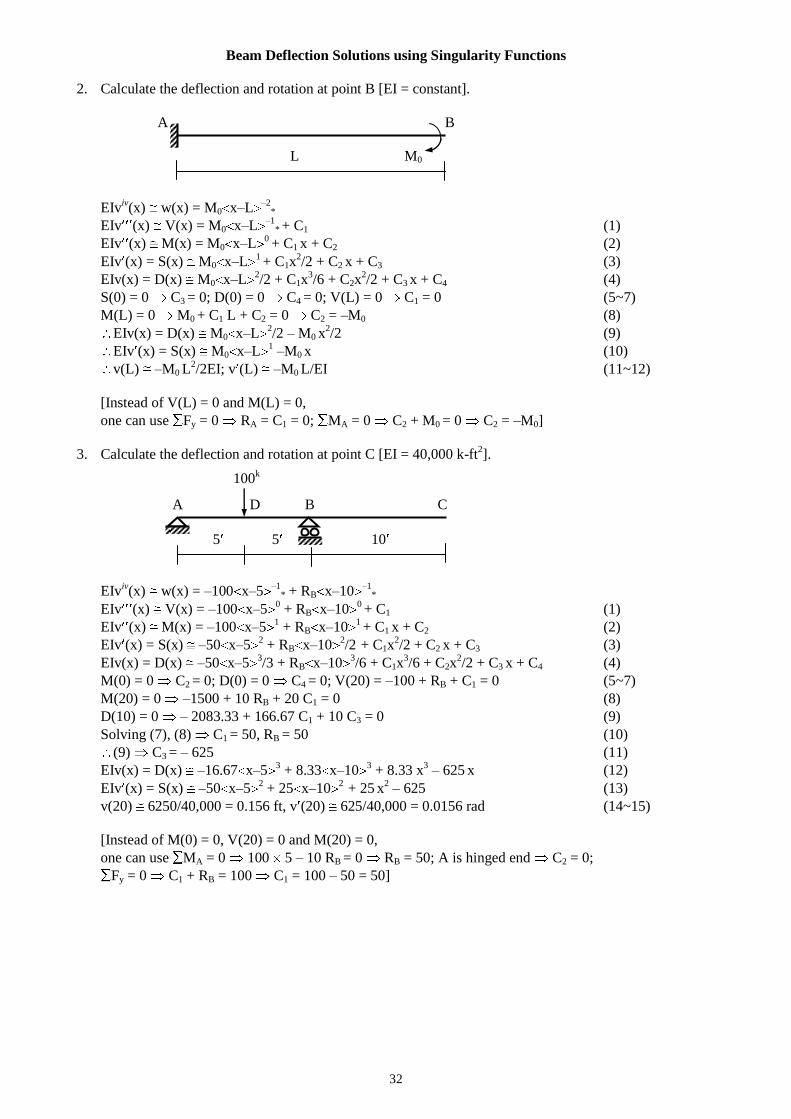
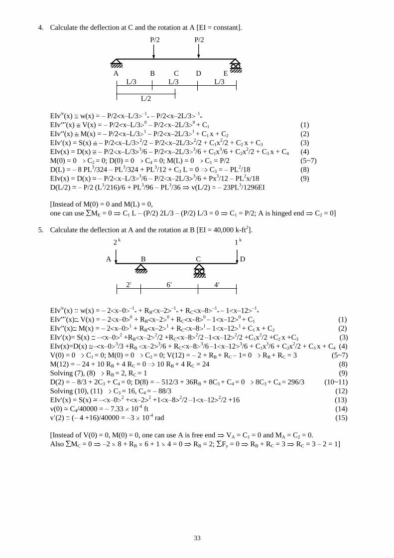
2. Calculate the deflection and rotation at point B [EI = constant].
A B
L M0
3. Calculate the deflection and rotation at point C [EI = 40,000 k-ft2].
100k
A D B C
5 5 10
4. Calculate the deflection at C and the rotation at A [EI = constant].
P/2 P/2
A B C D E
L/3 L/3 L/3
L/2
5. Calculate the deflection at A and the rotation at B [EI = 40,000 k-ft2].
2 k 1
k
A B C D
2 6 4
6. Calculate the deflection at A [EIAB = 40,000 k-ft2, EIBC = 20,000 k-ft
2].
2k/
A B C
3 6
7. Calculate the deflection at C [EIAB = EIDE = EI, EIBCD = 2EI].
P
A B C D E
L/3 L/3 L/3
L/2
8. Calculate the deflection at D [EI = constant].
P P
A B C D
L/2 L/2 L/2
31
9. Calculate the deflection at C and the rotation at B [EI= 40,000 k-ft2].
1 k/ft 2k
A B C
10 5
10. Calculate the deflection at B and rotations at the left and right of B [EI = 40,000 k-ft2].
2k
A B C D
5 5 5
11. Calculate the deflection at C [EI = constant].
P
A B C D
L/2 L/2 L
12. Calculate the deflection at B and rotations at the left and right of B [EI = constant].
w/unit length
A B C
L L
13. Calculate the reaction at support B [EI = constant].
10k
A B C
5 15
14. Calculate the deflection at B [EI = constant].
P
A B C D
L/2 L/2 L
15. Calculate the deflection at B and the rotation at C [EI= 40,000 k-ft2].
1.5 k/ft
A B C
10 10
32
Beam Deflection Solutions using Singularity Functions
2. Calculate the deflection and rotation at point B [EI = constant].
A B
L M0
EIviv(x) w(x) = M0 x–L
–2*
EIv (x) V(x) = M0 x–L–1
* + C1 (1)
EIv (x) M(x) = M0 x–L0 + C1 x + C2 (2)
EIv (x) = S(x) M0 x–L1 + C1x
2/2 + C2 x + C3 (3)
EIv(x) = D(x) M0 x–L2/2 + C1x
3/6 + C2x
2/2 + C3 x + C4 (4)
S(0) = 0 C3 = 0; D(0) = 0 C4 = 0; V(L) = 0 C1 = 0 (5~7)
M(L) = 0 M0 + C1 L + C2 = 0 C2 = –M0 (8)
EIv(x) = D(x) M0 x–L2/2 – M0 x
2/2 (9)
EIv (x) = S(x) M0 x–L1 –M0 x (10)
v(L) –M0 L2/2EI; v (L) –M0 L/EI (11~12)
[Instead of V(L) = 0 and M(L) = 0,
one can use Fy = 0 RA = C1 = 0; MA = 0 C2 + M0 = 0 C2 = –M0]
3. Calculate the deflection and rotation at point C [EI = 40,000 k-ft2].
A D B C
5 5 10
EIviv(x) w(x) = –100 x–5
–1* + RB x–10
–1*
EIv (x) V(x) = –100 x–50 + RB x–10
0 + C1 (1)
EIv (x) M(x) = –100 x–51 + RB x–10
1 + C1 x + C2 (2)
EIv (x) = S(x) –50 x–52 + RB x–10
2/2
+ C1x
2/2 + C2 x + C3 (3)
EIv(x) = D(x) –50 x–53/3 + RB x–10
3/6 + C1x
3/6 + C2x
2/2 + C3 x + C4 (4)
M(0) = 0 C2 = 0; D(0) = 0 C4 = 0; V(20) = –100 + RB + C1 = 0 (5~7)
M(20) = 0 –1500 + 10 RB + 20 C1 = 0 (8)
D(10) = 0 – 2083.33 + 166.67 C1 + 10 C3 = 0 (9)
Solving (7), (8) C1 = 50, RB = 50 (10)
(9) C3 = – 625 (11)
EIv(x) = D(x) –16.67 x–53 + 8.33 x–10
3 + 8.33 x
3 – 625 x (12)
EIv (x) = S(x) –50 x–52 + 25 x–10
2 + 25 x
2 – 625 (13)
v(20) 6250/40,000 = 0.156 ft, v (20) 625/40,000 = 0.0156 rad (14~15)
[Instead of M(0) = 0, V(20) = 0 and M(20) = 0,
one can use MA = 0 100 5 – 10 RB = 0 RB = 50; A is hinged end C2 = 0;
Fy = 0 C1 + RB = 100 C1 = 100 – 50 = 50]
100k
33
4. Calculate the deflection at C and the rotation at A [EI = constant].
P/2 P/2
A B C D E
L/3 L/3 L/3
L/2
EIviv(x) w(x) = – P/2 x–L/3
–1* – P/2 x–2L/3
–1*
EIv (x) V(x) = – P/2 x–L/30 – P/2 x–2L/3
0 + C1 (1)
EIv (x) M(x) = – P/2 x–L/31 – P/2 x–2L/3
1 + C1 x + C2 (2)
EIv (x) = S(x) – P/2 x–L/32/2 – P/2 x–2L/3
2/2 + C1x
2/2 + C2 x + C3 (3)
EIv(x) = D(x) – P/2 x–L/33/6 – P/2 x–2L/3
3/6 + C1x
3/6 + C2x
2/2 + C3 x + C4 (4)
M(0) = 0 C2 = 0; D(0) = 0 C4 = 0; M(L) = 0 C1 = P/2 (5~7)
D(L) = – 8 PL3/324 – PL
3/324 + PL
3/12 + C3 L = 0 C3 = – PL
2/18 (8)
EIv(x) = D(x) – P/2 x–L/33/6 – P/2 x–2L/3
3/6 + Px
3/12 – PL
2x/18 (9)
D(L/2) – P/2 (L3/216)/6 + PL
3/96 – PL
3/36 v(L/2) – 23PL
3/1296EI
[Instead of M(0) = 0 and M(L) = 0,
one can use ME = 0 C1 L – (P/2) 2L/3 – (P/2) L/3 = 0 C1 = P/2; A is hinged end C2 = 0]
5. Calculate the deflection at A and the rotation at B [EI = 40,000 k-ft2].
2 k 1
k
A B C D
2 6 4
EIviv(x) w(x) = – 2 x–0
–1* + RB x–2
–1* + RC x–8
–1* – 1 x–12
–1*
EIv (x) V(x) = – 2 x–00 + RB x–2
0 + RC x–8
0 – 1 x–12
0 + C1 (1)
EIv (x) M(x) = – 2 x–01 + RB x–2
1 + RC x–8
1 – 1 x–12
1 + C1 x + C2 (2)
EIv (x)= S(x) – x–02 +RB x–2
2/2 +RC x–8
2/2 –1 x–12
2/2 +C1x
2/2 +C2 x +C3 (3)
EIv(x)=D(x) – x–03/3 +RB x–2
3/6 + RC x–8
3/6 –1 x–12
3/6 + C1x
3/6 + C2x
2/2 + C3 x + C4 (4)
V(0) = 0 C1 = 0; M(0) = 0 C2 = 0; V(12) = – 2 + RB + RC – 1= 0 RB + RC = 3 (5~7)
M(12) = – 24 + 10 RB + 4 RC = 0 10 RB + 4 RC = 24 (8)
Solving (7), (8) RB = 2, RC = 1 (9)
D(2) = – 8/3 + 2C3 + C4 = 0; D(8) = – 512/3 + 36RB + 8C3 + C4 = 0 8C3 + C4 = 296/3 (10~11)
Solving (10), (11) C3 = 16, C4 = – 88/3 (12)
EIv (x) = S(x) – x–02 + x–2
2 +1 x–8
2/2 –1 x–12
2/2 +16 (13)
v(0) C4/40000 = – 7.33 10-4
ft (14)
v (2) (– 4 +16)/40000 = –3 10-4
rad (15)
[Instead of V(0) = 0, M(0) = 0, one can use A is free end VA = C1 = 0 and MA = C2 = 0.
Also MC = 0 –2 8 + RB 6 + 1 4 = 0 RB = 2; Fy = 0 RB + RC = 3 RC = 3 – 2 = 1]
34
8. Calculate the deflection at D [EI = constant].
P P
A B C D
L/2 L/2 L/2
EIviv(x) w(x) = – P x–L/2
–1* + RC x–L
–1* – P x–3L/2
–1*
EIv (x) V(x) = – P x–L/20 + RC x–L
0 – P x–3L/2
0 + C1 (1)
EIv (x) M(x) = – P x–L/21 + RC x–L
1– P x–3L/2
1 + C1 x + C2 (2)
EIv (x) = S(x) – P x–L/22/2 + RC x–L
2/2 – P x–3L/2
2/2 + C1x
2/2 + C2 x + C3 (3)
EIv(x) = D(x) – P x–L/23/6 + RC x–L
3/6 – P x–3L/2
3/6 + C1x
3/6 + C2x
2/2 + C3 x + C4 (4)
M(0) = 0 C2 = 0; D(0) = 0 C4 = 0; V(3L/2) = 0 RC + C1 = 2 P (5~7)
M(3L/2) = 0 – P L + RC L/2 + (3L/2) C1 = 0 (8)
Solving (7), (8) RC = 2P, C1 = 0 (9)
D(L) = – PL3/48 + C3 L = 0 C3 = PL
2/48 (10)
EIv(x) = D(x) – P x–L/23/6 + P x–L
3/3 – P x–3L/2
3/6 + PL
2x/48 (11)
v(3L/2) (– PL3/6 + PL
3/24 + PL
3/32)/EI = –3 PL
3/32 EI (12)
[Instead of M(0) = 0, V(3L/2) = 0 and M(3L/2) = 0, one can use
A is hinged end C2 = 0; MC = 0 C1 L + (P) L/2 – (P) L/2 = 0 C1 = 0;
Fy = 0 C1 + RC = 2P RC = 2P]
9. Calculate the deflection at C and the rotation at B [EI = 40,000 k-ft2].
1 k/ft 2k
A B C
10 5
EIviv(x) w(x) = –1 x–0
0 + 1 x–10
0 + RB x–10
–1* + 2 x–15
–1*
EIv (x) V(x) = –1 x–01 + 1 x–10
1 + RB x–10
0 + 2 x–15
0 + C1 (1)
EIv (x) M(x) = – x–02/2 + x–10
2/2 + RB x–10
1 + 2 x–15
1 + C1 x + C2 (2)
EIv (x) = S(x) – x–03/6 + x–10
3/6 + RB x–10
2/2 + x–15
2 + C1x
2/2 + C2 x + C3 (3)
EIv(x)=D(x) – x–04/24+ x–10
4/24+RB x–10
3/6+ x–15
3/3+C1x
3/6+C2x
2/2+C3 x+ C4 (4)
M(0) = 0 C2 = 0; D(0) = 0 C4 = 0; V(15) = –15 + 5 + RB + C1 + 2 = 0 RB + C1 = 8 (5~7)
M(15) = –112.5 + 12.5 + 5 RB + 15 C1 = 0 5 RB + 15 C1 = 100 (8)
Solving (7), (8) RB = 2, C1 = 6 (9)
D(10) = –104/24 + 6 10
3/6 + 10 C3 = 0 C3 = –58.33 (10)
EIv (x) = S(x) –x3/6 + x–10
3/6 + x–10
2 + x–15
2 + 3 x
2 – 58.33 (11)
EIv(x) = D(x) –x4/24 + x–10
4/24 + x–10
3/3 + x–15
3/3 + x
3– 58.33 x (12)
v (10) (–1000/6 + 300 – 58.33)/40000 = 1.875 10-3
rad (13)
v(15) (–50625/24 + 625/24 + 125/3 + 3375 – 875)/40000 = 11.46 10-3
ft (14)
[Instead of M(0) = 0, V(15) = 0 and M(15) = 0, one can use
A is hinged end C2 = 0; MB = 0 10 C1 – (1 10) 5 – 2 5 = 0 C1 = 6;
Fy = 0 C1 + RB – 10 + 2 = 0 RB = 2]
35
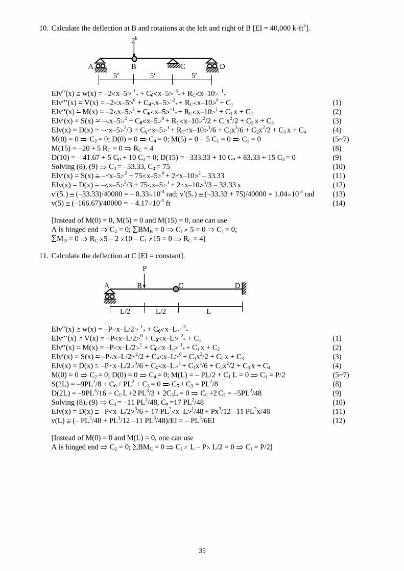
10. Calculate the deflection at B and rotations at the left and right of B [EI = 40,000 k-ft2].
2k
A B C D
5 5 5
EIviv(x) w(x) = –2 x–5
–1* + C x–5
–3* + RC x–10
–1*
EIv (x) V(x) = –2 x–50 + C x–5
–2* + RC x–10
0 + C1 (1)
EIv (x) M(x) = –2 x–51 + C x–5
–1* + RC x–10
1 + C1 x + C2 (2)
EIv (x) = S(x) – x–52 + C x–5
0 + RC x–10
2/2 + C1x
2/2 + C2 x + C3 (3)
EIv(x) = D(x) – x–53/3 + C x–5
1 + RC x–10
3/6 + C1x
3/6 + C2x
2/2 + C3 x + C4 (4)
M(0) = 0 C2 = 0; D(0) = 0 C4 = 0; M(5) = 0 + 5 C1 = 0 C1 = 0 (5~7)
M(15) = –20 + 5 RC = 0 RC = 4 (8)
D(10) = – 41.67 + 5 C + 10 C3 = 0; D(15) = –333.33 + 10 C + 83.33 + 15 C3 = 0 (9)
Solving (8), (9) C3 = –33.33, C = 75 (10)
EIv (x) = S(x) – x–52 + 75 x–5
0 + 2 x–10
2 – 33.33 (11)
EIv(x) = D(x) – x–53/3 + 75 x–5
1 + 2 x–10
3/3 – 33.33 x (12)
v (5–) (–33.33)/40000 = – 8.33 10-4
rad; v (5+) (–33.33 + 75)/40000 = 1.04 10-3
rad (13)
v(5) (–166.67)/40000 = – 4.17 10-3
ft (14)
[Instead of M(0) = 0, M(5) = 0 and M(15) = 0, one can use
A is hinged end C2 = 0; BMB = 0 C1 5 = 0 C1 = 0;
MD = 0 RC 5 – 2 10 – C1 15 = 0 RC = 4]
11. Calculate the deflection at C [EI = constant].
P
A B C D
L/2 L/2 L
EIviv(x) w(x) = –P x–L/2
–1* + C x–L
–3*
EIv (x) V(x) = –P x–L/20 + C x–L
–2* + C1 (1)
EIv (x) M(x) = –P x–L/21 + C x–L
–1* + C1 x + C2 (2)
EIv (x) = S(x) –P x–L/22/2 + C x–L
0 + C1x
2/2 + C2 x + C3 (3)
EIv(x) = D(x) –P x–L/23/6 + C x–L
1 + C1x
3/6 + C2x
2/2 + C3 x + C4 (4)
M(0) = 0 C2 = 0; D(0) = 0 C4 = 0; M(L) = – PL/2 + C1 L = 0 C1 = P/2 (5~7)
S(2L) = –9PL2/8 + C +
PL
2 + C3 = 0 C +
C3 = PL
2/8 (8)
D(2L) = –9PL3/16 + C L +2
PL
3/3 + 2C3L = 0 C +2
C3 = –5PL
2/48 (9)
Solving (8), (9) C3 = –11 PL2/48, C =17 PL
2/48 (10)
EIv(x) = D(x) –P x–L/23/6 + 17 PL
2x–L
1/48 + Px
3/12 –11 PL
2x/48 (11)
v(L) (– PL3/48 + PL
3/12 –11 PL
3/48)/EI = – PL
3/6EI (12)
[Instead of M(0) = 0 and M(L) = 0, one can use
A is hinged end C2 = 0; BMC = 0 C1 L – P L/2 = 0 C1 = P/2]
36
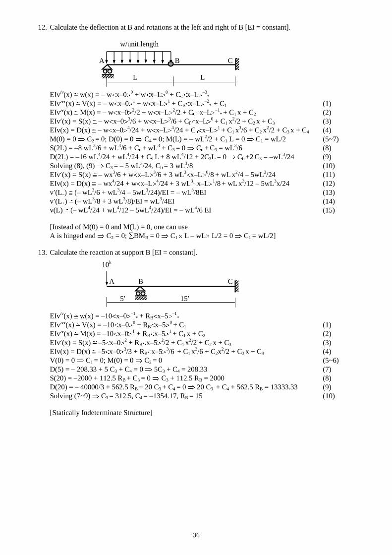
12. Calculate the deflection at B and rotations at the left and right of B [EI = constant].
w/unit length
A B C
L L
EIviv(x) w(x) = – w x–0
0 + w x–L
0 + C x–L
–3*
EIv (x) V(x) = – w x–01 + w x–L
1 + C x–L
–2* + C1 (1)
EIv (x) M(x) = – w x–02/2 + w x–L
2/2 + C x–L
–1* + C1 x + C2 (2)
EIv (x) = S(x) – w x–03/6 + w x–L
3/6 + C x–L
0 + C1 x
2/2 + C2 x + C3 (3)
EIv(x) = D(x) – w x–04/24 + w x–L
4/24 + C x–L
1 + C1 x
3/6 + C2 x
2/2 + C3 x + C4 (4)
M(0) = 0 C2 = 0; D(0) = 0 C4 = 0; M(L) = – wL2/2 + C1 L = 0 C1 = wL/2 (5~7)
S(2L) = –8 wL3/6 + wL
3/6 + C +
wL
3 + C3 = 0 C +
C3 = wL
3/6 (8)
D(2L) = –16 wL4/24 + wL
4/24 + C L + 8 wL
4/12 + 2C3L = 0 C +2
C3 = –wL
3/24 (9)
Solving (8), (9) C3 = – 5 wL3/24, C = 3 wL
3/8 (10)
EIv (x) = S(x) – wx3/6 + w x–L
3/6 + 3 wL
3x–L
0/8 + wL x
2/4 – 5wL
3/24 (11)
EIv(x) = D(x) – wx4/24 + w x–L
4/24 + 3 wL
3x–L
1/8 + wL x
3/12 – 5wL
3x/24 (12)
v (L–) (– wL3/6 + wL
3/4 – 5wL
3/24)/EI = – wL
3/8EI (13)
v (L+) (– wL3/8 + 3 wL
3/8)/EI = wL
3/4EI (14)
v(L) (– wL4/24 + wL
4/12 – 5wL
4/24)/EI = – wL
4/6 EI (15)
[Instead of M(0) = 0 and M(L) = 0, one can use
A is hinged end C2 = 0; BMB = 0 C1 L – wL L/2 = 0 C1 = wL/2]
13. Calculate the reaction at support B [EI = constant].
10k
A B C
5 15
EIviv(x) w(x) = –10 x–0
–1* + RB x–5
–1*
EIv (x) V(x) = –10 x–00 + RB x–5
0 + C1 (1)
EIv (x) M(x) = –10 x–01 + RB x–5
1 + C1 x + C2 (2)
EIv (x) = S(x) –5 x–02 + RB x–5
2/2 + C1 x
2/2 + C2 x + C3 (3)
EIv(x) = D(x) –5 x–03/3 + RB x–5
3/6 + C1 x
3/6 + C2x
2/2 + C3 x + C4 (4)
V(0) = 0 C1 = 0; M(0) = 0 C2 = 0 (5~6)
D(5) = – 208.33 + 5 C3 + C4 = 0 5C3 + C4 = 208.33 (7)
S(20) = –2000 + 112.5 RB + C3 = 0 C3 + 112.5 RB = 2000 (8)
D(20) = – 40000/3 + 562.5 RB + 20 C3 + C4 = 0 20 C3 + C4 + 562.5 RB = 13333.33 (9)
Solving (7~9) C3 = 312.5, C4 = –1354.17, RB = 15 (10)
[Statically Indeterminate Structure]
37
14. Calculate the deflection at B [EI = constant].
P
A B C D
L/2 L/2 L
EIviv(x) w(x) = –P x–L/2
–1* + RC x–L
–1*
EIv (x) V(x) = –P x–L/20 + RC x–L
0* + C1 (1)
EIv (x) M(x) = –P x–L/21 + RC x–L
1 + C1 x + C2 (2)
EIv (x) = S(x) –P x–L/22/2 + RC x–L
2/2 + C1x
2/2 + C2 x + C3 (3)
EIv(x) = D(x) –P x–L/23/6 + RC x–L
3/6 + C1x
3/6 + C2x
2/2 + C3 x + C4 (4)
M(0) = 0 C2 = 0; D(0) = 0 C4 = 0 (5~6)
M(2L) = –3PL/2 + RC L + 2C1 L = 0 RC + 2C1 = 3P/2 (7)
D(L) = – PL3/48 + C1 L
3/6 + C3 L = 0 C1 L
2/6 +
C3 = PL
2/48 (8)
D(2L) = –9PL3/16 + RC L
3/6 + 8C1 L
3/6 + 2C3 L = 0 RC L
2/6 + 4C1 L
2/3 +2C3 = 9PL
2/16 (9)
Solving (7~9) RC = 11 P/16; C1 = 13 P/32; C3 = –3PL2/64 (10)
EIv(x) = D(x) –P x–L/23/6 + 11 P x–L
3/96 + 13 Px
3/192 –3PL
2 x/64 (11)
v(L/2) (13 PL3/1536 –3 PL
3/128)/EI = –23 PL
3/1536 EI (12)
[Statically Indeterminate Structure]
15. Calculate the deflection at B and the rotation at C [EI = 40,000 k-ft2].
1.5 k/ft
A B C
10 10
EIviv(x) w(x) = –1.5 x–10
0
EIv (x) V(x) = –1.5 x–101 + C1 (1)
EIv (x) M(x) = –1.5 x–102/2 + C1 x + C2 (2)
EIv (x) = S(x) –1.5 x–103/6 + C1 x
2/2 + C2 x + C3 (3)
EIv(x) = D(x) –1.5 x–104/24 + C1 x
3/6 + C2 x
2/2 + C3 x + C4 (4)
S(0) = 0 C3 = 0; D(0) = 0 C4 = 0 (5~6)
M(20) = –75 + 20 C1 + C2 = 0 20 C1 + C2 = 75 (7)
D(20) = –625 + 1333.33 C1 + 200 C2 = 0 1333.33 C1 + 200 C2 = 625 (8)
Solving (7), (8) C1 = 5.39, C2 = –32.81 (10)
EIv (x) = S(x) –1.5 x–103/6 + 5.39 x
2/2 –32.81 x (11)
EIv(x) = D(x) –1.5 x–104/24 + 5.39 x
3/6 –32.81 x
2/2 (12)
v (20) (–250 + 1078 – 656.2)/40000 = 4.297 10-3
rad (13)
v(10) (898.44 –1640.62)/40000 = –18.55 10-3
ft (14)
[Statically Indeterminate Structure]
38
Moment-Area Theorems
The moment-curvature relationship Curvature = M/EI
For small deflection and slope, Curvature d2v/dx
2 = d /dx
d /dx = M/EI d = (M/EI) dx …………………………….(i)
Integrating Eq. (i) between A and B d = (M/EI) dx
B A = (M/EI) dx, where is integration between A and B ………………...….(ii)
Eq. (ii) The area under (M/EI) diagram between the points A and B is equal to the change of slope
between two points. This is the 1st Moment-Area Theorem.
Multiplying both sides of Eq. (i) by x x d = x (M/EI) dx ……………………(iii)
Integrating Eq. (iii) between A and B x d = x (M/EI) dx
(xB xA) B (vB vA) = x (M/EI) dx, where is integration between A and B ………...(iv)
Example 1: Calculate the tip rotation and deflection of the cantilever beam shown below [EI = const].
B A = Area of M/EI diagram between A an B
= ( P0L/EI) L/2 = P0L2/2EI
A = P0L
2/2EI …………..(1)
(xB xA) B (vB vA) = ( P0L/EI) L/2 2L/3
L 0
0 + vA P0L3/3EI
vA = P0L
3/3EI …………..(2)
Example 2: Calculate the end rotation and midspan deflection of the simply supported beam shown below.
B A = (P0L/4EI) L/2 = P0L2/8EI …………..(1)
(xB xA) B (vB vA) = (P0L/4EI) L/2 L/2
L B
0 + 0 = P0L3/16EI
B = P0L
2/16EI; Eq. (1) A
= P0L
2/16EI ………..(2)
(xC xA) C (vC vA) = (P0L/4EI) L/4 L/3
L/2 0
vC + 0 = P0L3/48EI
vC = P0L3/48EI ………....(3)
L
B
(xB xA) B
(vB vA)
A
B
(xB xA)
The figure at right shows the geometric
significance of various terms in Eq. (iv).
Eq. (iv) The moment of the area under
(M/EI) diagram between the points A and B
(i.e., x (M/EI) dx) equals to the deflection
of A with respect to the tangent at B; i.e.,
tA/B. This is the 2nd
Moment-Area Theorem.
tA/B
P0L/EI
P0
L/2 L/2
A B
P0L/4EI
C
A B
P0
39
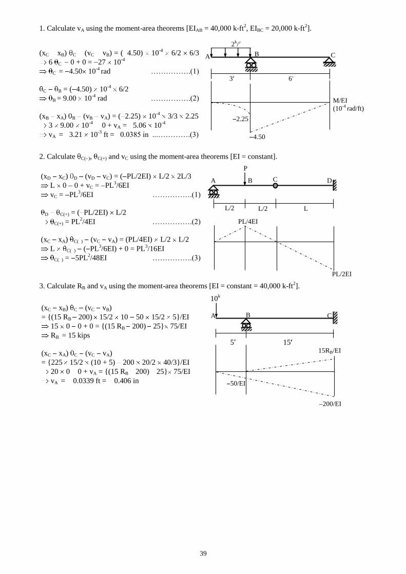
1. Calculate vA using the moment-area theorems [EIAB = 40,000 k-ft2, EIBC = 20,000 k-ft
2].
3 6
2. Calculate C( ), C(+) and vC using the moment-area theorems [EI = constant].
3. Calculate RB and vA using the moment-area theorems [EI = constant = 40,000 k-ft2].
10k
5 15
2.25
C A B
2k/
4.50
(xC xB) C (vC vB) = ( 4.50) 10-4
6/2 6/3
6 C
0 + 0 = 27 10-4
C = 4.50 10
-4 rad …………….(1)
C B = ( 4.50) 10-4
6/2
B = 9.00 10
-4 rad …………….(2)
(xB xA) B (vB vA) = ( 2.25) 10-4
3/3 2.25
3 9.00 10-4
0 + vA = 5.06 10-4
vA = 3.21 10
-3 ft = 0.0385 in ...………….(3)
P
A B C D
L/2 L/2 L
(xD xC) D (vD vC) = ( PL/2EI) L/2 2L/3
L 0 0 + vC = PL3/6EI
vC = PL3/6EI …………….(1)
D C(+) = ( PL/2EI) L/2
C(+) = PL2/4EI …………….(2)
(xC xA) C( ) (vC vA) = (PL/4EI) L/2 L/2
L C( ) ( PL3/6EI) + 0 = PL
3/16EI
C( ) = 5PL2/48EI …………….(3)
PL/4EI
PL/2EI
A B C
15RB/EI
200/EI
(xC xB) C (vC vB)
= {(15 RB 200) 15/2 10 50 15/2 5}/EI
15 0 0 + 0 = {(15 RB 200) 25} 75/EI
RB = 15 kips
(xC xA) C (vC vA)
= {225 15/2 (10 + 5) 200 20/2 40/3}/EI
20 0 0 + vA = {(15 RB 200) 25} 75/EI
vA = 0.0339 ft = 0.406 in
50/EI
M/EI
(10-4
rad/ft)
40
Beam Deflection Solutions using Moment-Area Theorems
2. Calculate the deflection and rotation at point B [EI = constant].
A B
L M0 M0/EI
Between A and B, A = 0, vA = 0
1st theorem B A = L ( M0/EI) = M0L/EI B = M0L/EI ……….(1)
and 2nd
theorem L B vB + vA = ( M0 L/EI) L/2 = M0L2/2EI vB = M0L
2/2EI ………(2)
3. Calculate the deflection and rotation at point C [EI = 40,000 k-ft2].
A D B C
5 5 10
Between A and B, vA = 0, vB = 0
1st theorem B A = 10/2 6.25 10
3 = 31.25 10
3 ……….(1)
and 2nd
theorem 10 B vB + vA = 31.25 103 10/2 B = 15.63 10
3 rad ……….(2)
Between B and C, B = 15.63 103 rad, vB = 0
1st theorem C B = 0 C = 0.0156 rad ……….(3)
and 2nd
theorem 10 C vC + vB = 0 vC = 0.156 ft ……….(4)
4. Calculate the deflection at C and the rotation at A [EI = constant].
P/2 P/2
A E
B C D
L/2
Using symmetry between A and C, vA = 0, C = 0
1st theorem C A = L/6 PL/6EI + L/6 PL/6EI
= PL
2/18EI A = PL
2/18EI ....…….(1)
and 2nd
theorem (L/2) C vC + vA= PL2/36 EI (2L/9) + PL
2/36 EI (L/3+L/12)
= 23 PL
3/1296 EI
vC = 23 PL3/1296 EI ……….(2)
5. Calculate the deflection at A and the rotation at B [EI = 40,000 k-ft2].
2 k 1
k
A B C D
2 6 4
Between B and C, vB = 0, vC = 0
1st theorem C B = 6 ( 10
4) = 6 10
4 ……….(1)
and 2nd
theorem 6 C vC + vB = ( 6 104) 6/2 C = 3 10
4 rad ……….(2)
(1) B = 3 104 rad ...…….(1)
Between A and B, B = 3 104 rad, vB = 0
1st theorem B A = 2/2 ( 10
4) = 10
4 A = 4 10
4 rad ……….(3)
and 2nd
theorem 2 B vB + vA = 104 4/3 vA = 7.33 10
4 ft ……….(4)
100k 6.25 10
3 rad/ft
PL/6EI PL/6EI
104 rad/ft 10
4 rad/ft
L/3 L/3 L/3
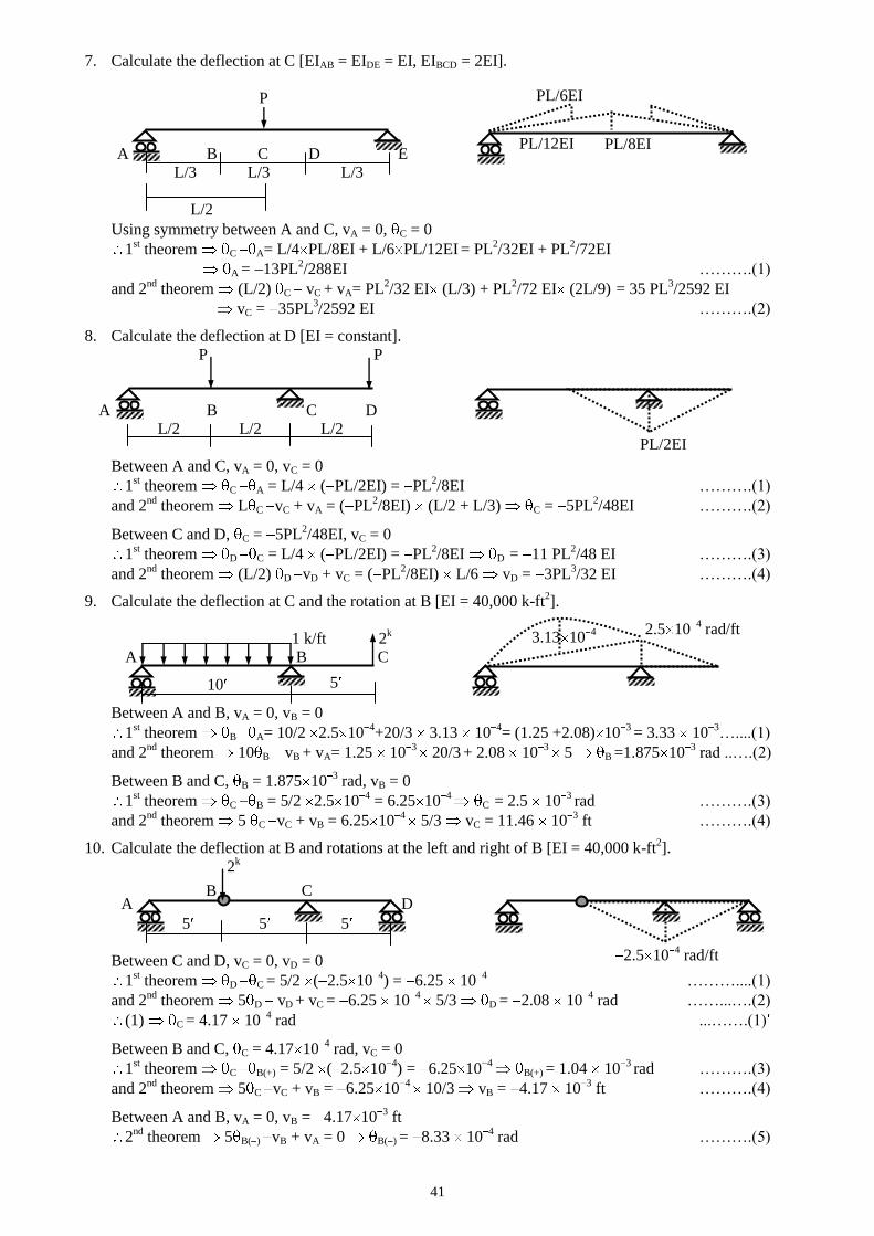
41
7. Calculate the deflection at C [EIAB = EIDE = EI, EIBCD = 2EI].
P
A B C D E
L/3 L/3 L/3
L/2
Using symmetry between A and C, vA = 0, C = 0
1st theorem C A= L/4 PL/8EI + L/6 PL/12EI
= PL
2/32EI + PL
2/72EI
A = 13PL2/288EI ……….(1)
and 2nd
theorem (L/2) C vC + vA= PL2/32 EI (L/3) + PL
2/72 EI (2L/9)
= 35 PL
3/2592 EI
vC = 35PL3/2592 EI ……….(2)
8. Calculate the deflection at D [EI = constant].
P P
A B C D
L/2 L/2 L/2
Between A and C, vA = 0, vC = 0
1st theorem C A = L/4 ( PL/2EI) = PL
2/8EI ……….(1)
and 2nd
theorem L C vC + vA = ( PL2/8EI) (L/2 + L/3) C = 5PL
2/48EI ……….(2)
Between C and D, C = 5PL2/48EI, vC = 0
1st theorem D C = L/4 ( PL/2EI) = PL
2/8EI D = 11 PL
2/48 EI ……….(3)
and 2nd
theorem (L/2) D vD + vC = ( PL2/8EI) L/6 vD = 3PL
3/32 EI ……….(4)
9. Calculate the deflection at C and the rotation at B [EI = 40,000 k-ft2].
1 k/ft 2k
A B C
Between A and B, vA = 0, vB = 0
1st theorem B A= 10/2 2.5 10
4+20/3 3.13 10
4= (1.25 +2.08) 10
3 = 3.33 10
3…....(1)
and 2nd
theorem 10 B vB + vA= 1.25 103
20/3 + 2.08 10
3 5 B =1.875 10
3 rad ..….(2)
Between B and C, B = 1.875 103 rad, vB = 0
1st theorem C B = 5/2 2.5 10
4 = 6.25 10
4 C = 2.5 10
3 rad ……….(3)
and 2nd
theorem 5 C vC + vB = 6.25 104
5/3 vC = 11.46 103 ft ……….(4)
10. Calculate the deflection at B and rotations at the left and right of B [EI = 40,000 k-ft2].
2k
A D
5 5 5
Between C and D, vC = 0, vD = 0
1st theorem D C = 5/2 ( 2.5 10
4) = 6.25 10
4 ………....(1)
and 2nd
theorem 5 D vD + vC = 6.25 104
5/3 D = 2.08 104 rad ……...….(2)
(1) C = 4.17 104 rad ...…….(1)
Between B and C, C = 4.17 104 rad, vC = 0
1st theorem C B(+) = 5/2 ( 2.5 10
4) = 6.25 10
4 B(+) = 1.04 10
3 rad ……….(3)
and 2nd
theorem 5 C vC + vB = 6.25 104
10/3 vB = 4.17 103 ft ……….(4)
Between A and B, vA = 0, vB = 4.17 103 ft
2nd
theorem 5 B( ) vB + vA = 0 B( ) = 8.33 104 rad ……….(5)
3.13 104
PL/2EI
2.5 104 rad/ft
PL/6EI
PL/12EI PL/8EI
10 5
2.5 104 rad/ft
B
C
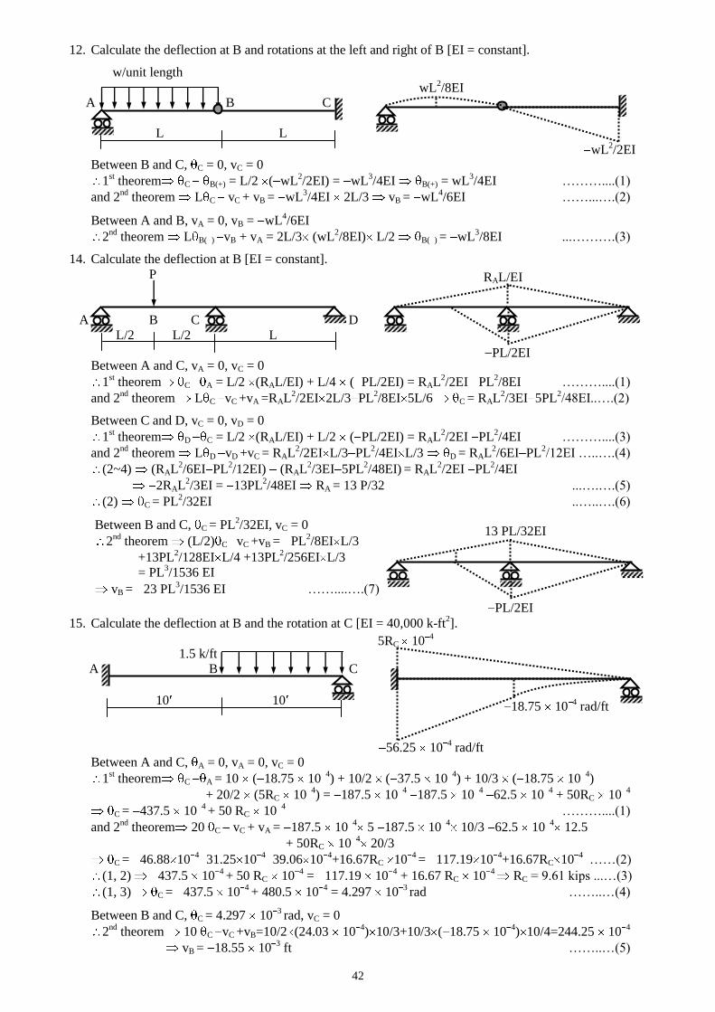
42
12. Calculate the deflection at B and rotations at the left and right of B [EI = constant].
w/unit length
A B C
L L
Between B and C, C = 0, vC = 0
1st theorem C B(+) = L/2 ( wL
2/2EI) = wL
3/4EI B(+) = wL
3/4EI ………....(1)
and 2nd
theorem L C vC + vB = wL3/4EI 2L/3 vB = wL
4/6EI ……...….(2)
Between A and B, vA = 0, vB = wL4/6EI
2nd
theorem L B( ) vB + vA = 2L/3 (wL2/8EI) L/2 B( ) = wL
3/8EI ...……….(3)
14. Calculate the deflection at B [EI = constant].
P
A B C D
L/2 L/2 L
Between A and C, vA = 0, vC = 0
1st theorem C A = L/2 (RAL/EI) + L/4 ( PL/2EI) = RAL
2/2EI PL
2/8EI ………....(1)
and 2nd
theorem L C vC +vA =RAL2/2EI 2L/3 PL
2/8EI 5L/6 C = RAL
2/3EI 5PL
2/48EI..….(2)
Between C and D, vC = 0, vD = 0
1st theorem D C = L/2 (RAL/EI) + L/2 ( PL/2EI) = RAL
2/2EI PL
2/4EI ………....(3)
and 2nd
theorem L D vD +vC = RAL2/2EI L/3 PL
2/4EI L/3 D = RAL
2/6EI PL
2/12EI …..….(4)
(2~4) (RAL2/6EI PL
2/12EI) (RAL
2/3EI 5PL
2/48EI) = RAL
2/2EI PL
2/4EI
2RAL2/3EI = 13PL
2/48EI RA = 13 P/32 ...….….(5)
(2) C = PL2/32EI ..…..….(6)
15. Calculate the deflection at B and the rotation at C [EI = 40,000 k-ft2].
1.5 k/ft
A B C
10 10
Between A and C, A = 0, vA = 0, vC = 0
1st theorem C A = 10 ( 18.75 10
4) + 10/2 ( 37.5 10
4) + 10/3 ( 18.75 10
4)
+ 20/2 (5RC 104) = 187.5 10
4 187.5 10
4 62.5 10
4 + 50RC 10
4
C = 437.5 104 + 50 RC 10
4 ………....(1)
and 2nd
theorem 20 C vC + vA = 187.5 104
5 187.5 104
10/3 62.5 104
12.5
+ 50RC 104
20/3
C = 46.88 104
31.25 104
39.06 104+16.67RC 10
4 = 117.19 10
4+16.67RC 10
4 ……(2)
(1, 2) 437.5 104 + 50 RC 10
4 = 117.19 10
4 + 16.67 RC 10
4 RC = 9.61 kips ...…(3)
(1, 3) C = 437.5 104 + 480.5 10
4 = 4.297 10
3 rad ……..…(4)
Between B and C, C = 4.297 103 rad, vC = 0
2nd
theorem 10 C vC +vB=10/2 (24.03 104) 10/3+10/3 ( 18.75 10
4) 10/4=244.25 10
4
vB = 18.55 103 ft ……..…(5)
wL2/8EI
wL2/2EI
PL/2EI
RAL/EI
PL/2EI
13 PL/32EI Between B and C, C = PL
2/32EI, vC = 0
2nd
theorem (L/2) C vC +vB = PL2/8EI L/3
+13PL2/128EI L/4 +13PL
2/256EI L/3
= PL3/1536 EI
vB = 23 PL3/1536 EI ……....….(7)
18.75 104 rad/ft
56.25 104 rad/ft
5RC 104
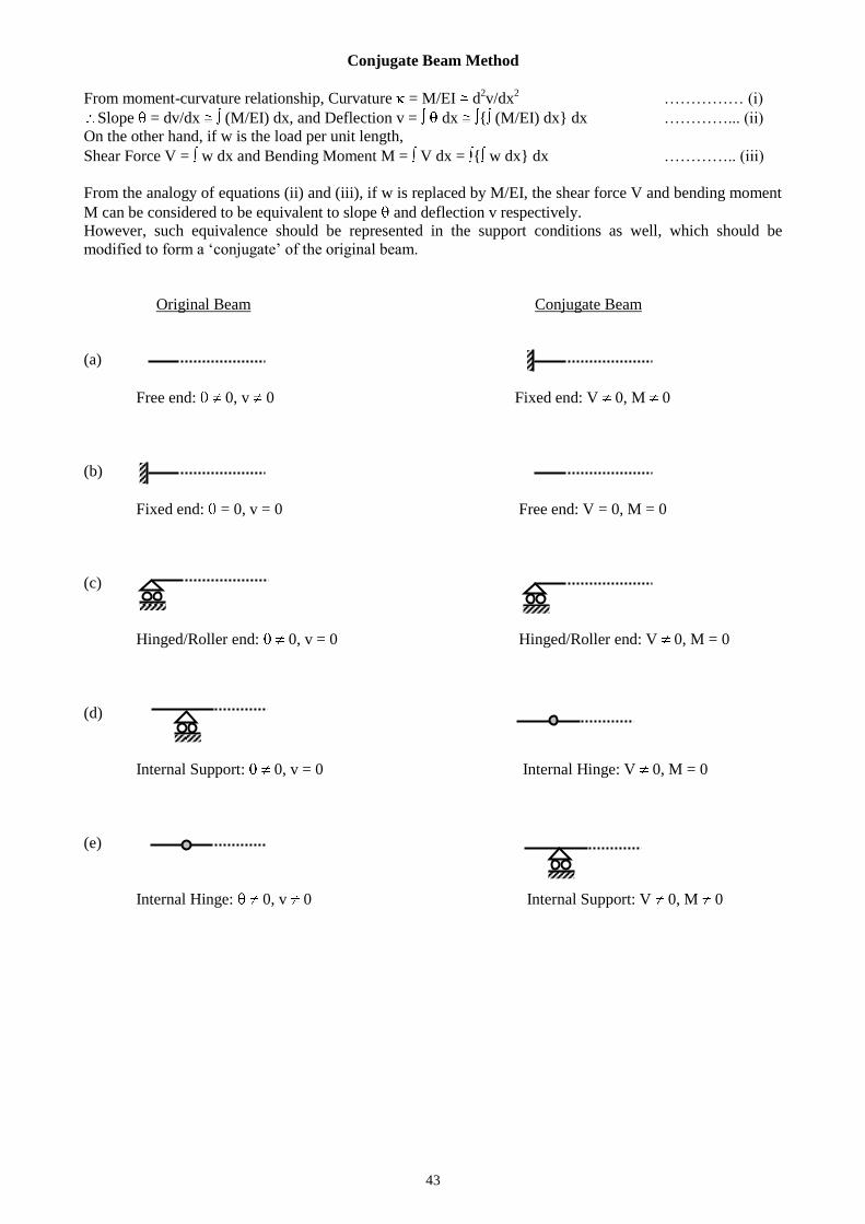
43
Conjugate Beam Method
From moment-curvature relationship, Curvature = M/EI d2v/dx
2 …………… (i)
Slope = dv/dx (M/EI) dx, and Deflection v = dx { (M/EI) dx} dx …………... (ii)
On the other hand, if w is the load per unit length,
Shear Force V = w dx and Bending Moment M = V dx = { w dx} dx ………….. (iii)
From the analogy of equations (ii) and (iii), if w is replaced by M/EI, the shear force V and bending moment
M can be considered to be equivalent to slope and deflection v respectively.
However, such equivalence should be represented in the support conditions as well, which should be
modified to form a ‘conjugate’ of the original beam.
Original Beam Conjugate Beam
(a)
Free end: 0, v 0 Fixed end: V 0, M 0
(b)
Fixed end: = 0, v = 0 Free end: V = 0, M = 0
(c)
Hinged/Roller end: 0, v = 0 Hinged/Roller end: V 0, M = 0
(d)
Internal Support: 0, v = 0 Internal Hinge: V 0, M = 0
(e)
Internal Hinge: 0, v 0 Internal Support: V 0, M 0
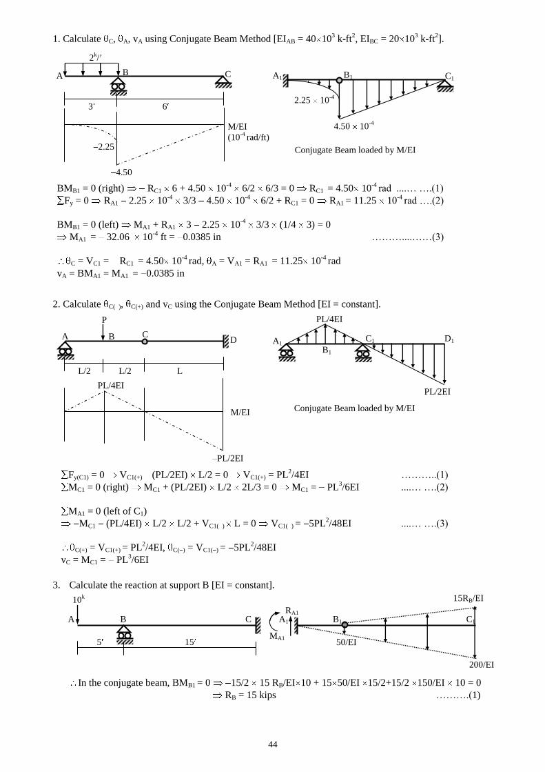
44
1. Calculate C, A, vA using Conjugate Beam Method [EIAB = 40 103 k-ft
2, EIBC = 20 10
3 k-ft
2].
3 6
2. Calculate C( ), C(+) and vC using the Conjugate Beam Method [EI = constant].
L/2 L/2 L
3. Calculate the reaction at support B [EI = constant].
A B C A1 B1 C1
5 15
In the conjugate beam, BMB1 = 0 15/2 15 RB/EI 10 + 15 50/EI 15/2+15/2 150/EI 10 = 0
RB = 15 kips ……….(1)
2.25
C A B
2k/
4.50
M/EI
(10-4
rad/ft)
2.25 10-4
C1 A1 B1
4.50 10-4
BMB1 = 0 (right) RC1 6 + 4.50 10-4
6/2 6/3 = 0 RC1 = 4.50 10
-4 rad ....… ….(1)
Fy = 0 RA1 2.25 10-4
3/3 4.50 10-4
6/2 + RC1 = 0 RA1 = 11.25 10
-4 rad ….(2)
BMB1 = 0 (left) MA1 + RA1 3 2.25 10-4
3/3 (1/4 3) = 0
MA1 = 32.06 10
-4 ft = 0.0385 in ………....……(3)
C = VC1 = RC1 = 4.50 10
-4 rad, A = VA1 = RA1
= 11.25 10
-4 rad
vA = BMA1 = MA1 = 0.0385 in
D A C
P
M/EI
D1 A1 B1
Fy(C1) = 0 VC1(+) (PL/2EI) L/2 = 0 VC1(+) = PL2/4EI ………..(1)
MC1 = 0 (right) MC1 + (PL/2EI) L/2 2L/3 = 0 MC1 = PL3/6EI ....… ….(2)
MA1 = 0 (left of C1)
MC1 (PL/4EI) L/2 L/2 + VC1( ) L = 0 VC1( ) = 5PL2/48EI ....… ….(3)
C(+) = VC1(+) = PL2/4EI, C( ) = VC1( ) = 5PL
2/48EI
vC = MC1 = PL3/6EI
B
PL/2EI
C1
PL/4EI
Conjugate Beam loaded by M/EI
Conjugate Beam loaded by M/EI
PL/2EI
PL/4EI
200/EI
15RB/EI
50/EI
RA1
MA1
10k
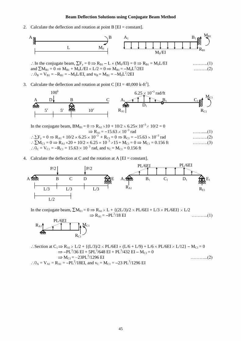
45
Beam Deflection Solutions using Conjugate Beam Method
2. Calculate the deflection and rotation at point B [EI = constant].
A B A1 B1
L M0
In the conjugate beam, Fy = 0 RB1 L (M0/EI) = 0 RB1 = M0L/EI ……….(1)
and MB1 = 0 MB1 + M0L/EI L/2 = 0 MB1 = M0L2/2EI ………(2)
B = VB1 = RB1 = M0L/EI, and vB = MB1 = M0L2/2EI
3. Calculate the deflection and rotation at point C [EI = 40,000 k-ft2].
A D B C A1 B1 C1
D1
5 5 10
In the conjugate beam, BMB1 = 0 RA1 10 + 10/2 6.25 103
10/2 = 0
RA1 = 15.63 103 rad …….....(1)
Fy = 0 RA1 + 10/2 6.25 103 + RC1
= 0 RC1 = 15.63 10
3 rad ……….(2)
MC1 = 0 RA1 20 + 10/2 6.25 103 15 + MC1
= 0 MC1 = 0.156 ft ……….(3)
C = VC1 = RC1 = 15.63 103 rad, and vC = MC1 = 0.156 ft
4. Calculate the deflection at C and the rotation at A [EI = constant].
P/2 P/2
A B C D E A1 B1 C1 D1 E1
L/3 L/3 L/3
L/2
In the conjugate beam, ME1 = 0 RA1 L + {(2L/3)/2 PL/6EI + L/3 PL/6EI} L/2
RA1 = PL2/18 EI ………..(1)
Section at C1 RA1 L/2 + {(L/3)/2 PL/6EI (L/6 + L/9) + L/6 PL/6EI L/12} MC1 = 0
PL3/36 EI + 5PL
3/648 EI + PL
3/432 EI MC1
= 0
MC1 = 23PL
3/1296 EI ………...(2)
A = VA1 = RA1 = PL2/18EI, and vC = MC1 = 23 PL
3/1296 EI
M0/EI
100k 6.25 10
3 rad/ft
PL/6EI PL/6EI
MB1
RB1
MC1
RC1 RA1
RE1 RA1
PL/6EI RA1 MC1
RC1
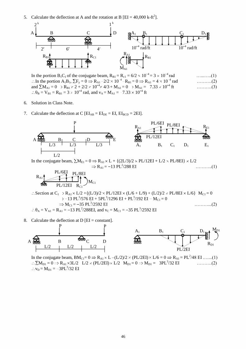
46
5. Calculate the deflection at A and the rotation at B [EI = 40,000 k-ft2].
A B C D A1 B1 C1 D1
2 6 4
In the portion B1C1 of the conjugate beam, RB1 = Rc1 = 6/2 104 = 3 10
4 rad …...…..(1)
In the portion A1B1, Fy = 0 RA1 2/2 104
RB1 = 0 RA1 = 4 10
4 rad ……….(2)
and MA1 = 0 RB1 2 + 2/2 104
4/3 + MA1 = 0 MA1 = 7.33 10
4 ft ……….(3)
B = VB1 = RB1 = 3 104 rad, and vA = MA1 = 7.33 10
4 ft
6. Solution in Class Note.
7. Calculate the deflection at C [EIAB = EIDE = EI, EIBCD = 2EI].
A B C D E
L/3 L/3 L/3 A1 B1 C1 D1 E1
L/2
In the conjugate beam, ME1 = 0 RA1 L + {(2L/3)/2 PL/12EI + L/2 PL/8EI} L/2
RA1 = 13 PL2/288 EI ………..(1)
Section at C1 RA1 L/2 +{(L/3)/2 PL/12EI (L/6 + L/9) + (L/2)/2 PL/8EI L/6} MC1 = 0
13 PL3/576 EI + 5PL
3/1296 EI + PL
3/192 EI MC1
= 0
MC1 = 35 PL
3/2592 EI ………...(2)
A = VA1 = RA1 = 13 PL2/288EI, and vC = MC1 = 35 PL
3/2592 EI
8. Calculate the deflection at D [EI = constant].
A1 B1 C1 D1
A B C D
L/2 L/2 L/2
In the conjugate beam, BMC1= 0 RA1 L (L/2)/2 (PL/2EI)
L/6 = 0 RA1 = PL2/48 EI .…...(1)
MD1 = 0 RA1 3L/2 L/2 (PL/2EI)
L/2 MD1 = 0 MD1 = 3PL
3/32 EI ……….(2)
vD = MD1 = 3PL3/32 EI
104 rad/ft
PL/2EI
104 rad/ft
PL/6EI
PL/12EI
PL/8EI
2 k 1
k
RB1 RC1 RB1 RA1
MA1
MD1
RD1
P RA1 RE1
PL/6EI RA1
MC1 RC1 PL/12EI
PL/8EI
P P
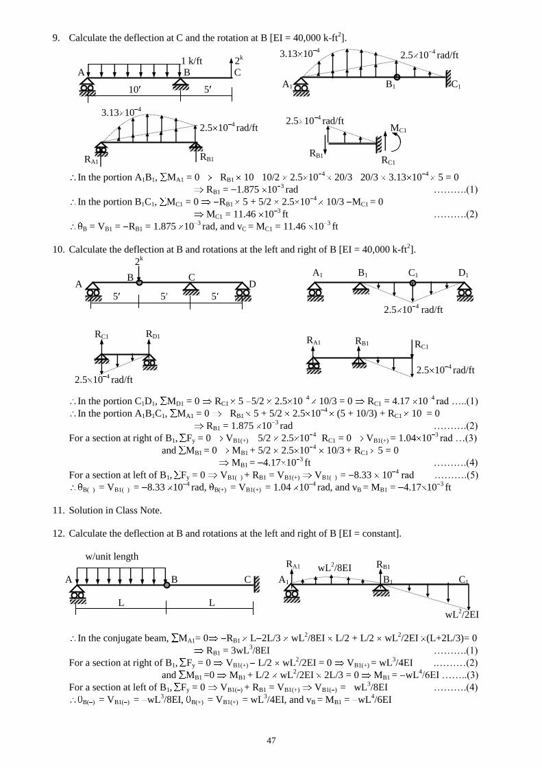
47
9. Calculate the deflection at C and the rotation at B [EI = 40,000 k-ft2].
1 k/ft 2k
A B C
A1 B1 C1
In the portion A1B1, MA1 = 0 RB1 10 10/2 2.5 104
20/3 20/3 3.13 104
5 = 0
RB1 = 1.875 103 rad ……….(1)
In the portion B1C1, MC1 = 0 RB1 5 + 5/2 2.5 104
10/3 MC1 = 0
MC1 = 11.46 103 ft ……….(2)
B = VB1 = RB1 = 1.875 103 rad, and vC = MC1 = 11.46 10
3 ft
10. Calculate the deflection at B and rotations at the left and right of B [EI = 40,000 k-ft2].
A1 B1 C1 D1
A D
5 5 5
In the portion C1D1, MD1 = 0 RC1 5 5/2 2.5 104
10/3 = 0 RC1 = 4.17 104 rad …..(1)
In the portion A1B1C1, MA1 = 0 RB1 5 + 5/2 2.5 104
(5 + 10/3) + RC1 10 = 0
RB1 = 1.875 103 rad ……….(2)
For a section at right of B1, Fy = 0 VB1(+) 5/2 2.5 104
RC1 = 0 VB1(+) = 1.04 103 rad …(3)
and MB1 = 0 MB1 + 5/2 2.5 104 10/3
+ RC1 5 = 0
MB1 = 4.17 103 ft ……….(4)
For a section at left of B1, Fy = 0 VB1( ) + RB1 = VB1(+) VB1( ) = 8.33 104 rad ……….(5)
B( ) = VB1( ) = 8.33 104 rad, B(+) = VB1(+) = 1.04 10
4 rad, and vB = MB1 = 4.17 10
3 ft
11. Solution in Class Note.
12. Calculate the deflection at B and rotations at the left and right of B [EI = constant].
w/unit length
A B C A1 B1 C1
L L
In the conjugate beam, MA1= 0 RB1 L 2L/3 wL2/8EI L/2 + L/2 wL
2/2EI (L+2L/3)= 0
RB1 = 3wL3/8EI ……….(1)
For a section at right of B1, Fy = 0 VB1(+) L/2 wL2/2EI = 0 VB1(+) = wL
3/4EI .………(2)
and MB1 =0 MB1 + L/2 wL2/2EI 2L/3 = 0 MB1 = wL
4/6EI ……..(3)
For a section at left of B1, Fy = 0 VB1( ) + RB1 = VB1(+) VB1( ) = wL3/8EI ……….(4)
B( ) = VB1( ) = wL3/8EI, B(+) = VB1(+) = wL
3/4EI, and vB = MB1 = wL
4/6EI
3.13 104
wL2/8EI
wL2/2EI
10 5
3.13 104
C
2.5 104 rad/ft
2.5 104 rad/ft
2.5 104 rad/ft
RA1 RB1 RB1
MC1
RC1
2.5 104 rad/ft
2.5 104 rad/ft
2.5 104 rad/ft
RC1 RD1 RA1 RB1 RC1
2k
B
RA1 RB1

48
13. Solution in Class Note.
14. Calculate the deflection at B [EI = constant].
A B C D B1 C1
L/2 L/2 L
In the conjugate beam, BMC1 = 0 RA1 L + L/2 RAL/EI L/3 L/4 PL/2EI L/6 = 0
RA1 = RAL2/6EI + PL
2/48EI ……….(1)
Also, BMC1 = 0 RD1 L L/2 RAL/EI L/3 + L/2 PL/2EI L/3 = 0
RD1 = RAL2/6EI + PL
2/12EI ……….(2)
Fy = 0 RA1 + RD1 = (2L/2) RAL/EI + 3L/4 PL/2EI = RAL2/EI + 3 PL
2/8EI ………..(3)
[(1) + (2)], (3) RAL2/3EI + 5PL
2/48EI = RAL
2/EI + 3PL
2/8EI
2RAL2/3EI = 13 PL
2/48EI RA = 13 P/32 ……….(4)
(1) RA1 = RAL2/6EI + PL
2/48EI = 13PL
2/192EI + PL
2/48EI = 3PL
2/64EI ……….(5)
Section at B1 RA1 L/2 + L/4 RAL/2EI L/6 MB1 = 0
MB1 = 3PL
3/128EI + 13PL
3/1536EI = 23PL
3/1536EI ……….(6)
vB = MB1 = 23PL3/1536EI
15. Calculate the deflection at B and the rotation at C [EI = 40,000 k-ft2].
A B C A1 B1 C1
10 10
In the conjugate beam, MC1 = 0 20/2 5RC 104
40/3 + 10/3 18.75 104
30/4
+ 10 18.75 104
(10+5) + 10/2 37.5 104
(10 +20/3) = 0
666.67 RC = 6406.25 RC = 9.61 kips ……….(1)
Fy = 0 RC1 + 20/2 5 9.61 104
10/3 18.75 104
10/2 (18.75 + 56.25) 104 = 0
RC1 = 4.297 103 rad ………..(2)
Section at B1 (right)
RC1 10 10/2 2.5 9.61 104 10/3 + 10/3 18.75 10
4 10/4 + MB1
= 0
MB1 = 4.297 10
3 10 + 10/2 2.5 9.61 10
4 10/3 10/3 18.75 10
4 10/4 …….(3)
= 18.55 103 ft
C = VC1 = RC1 = 4.297 103 rad, vB = MB1 = 18.55 10
3 ft
PL/2EI
RAL/EI
18.75 104 rad/ft
56.25 104 rad/ft
5RC 104
P
D1 A1
RA1 RD1
1.5 k/ft RC1
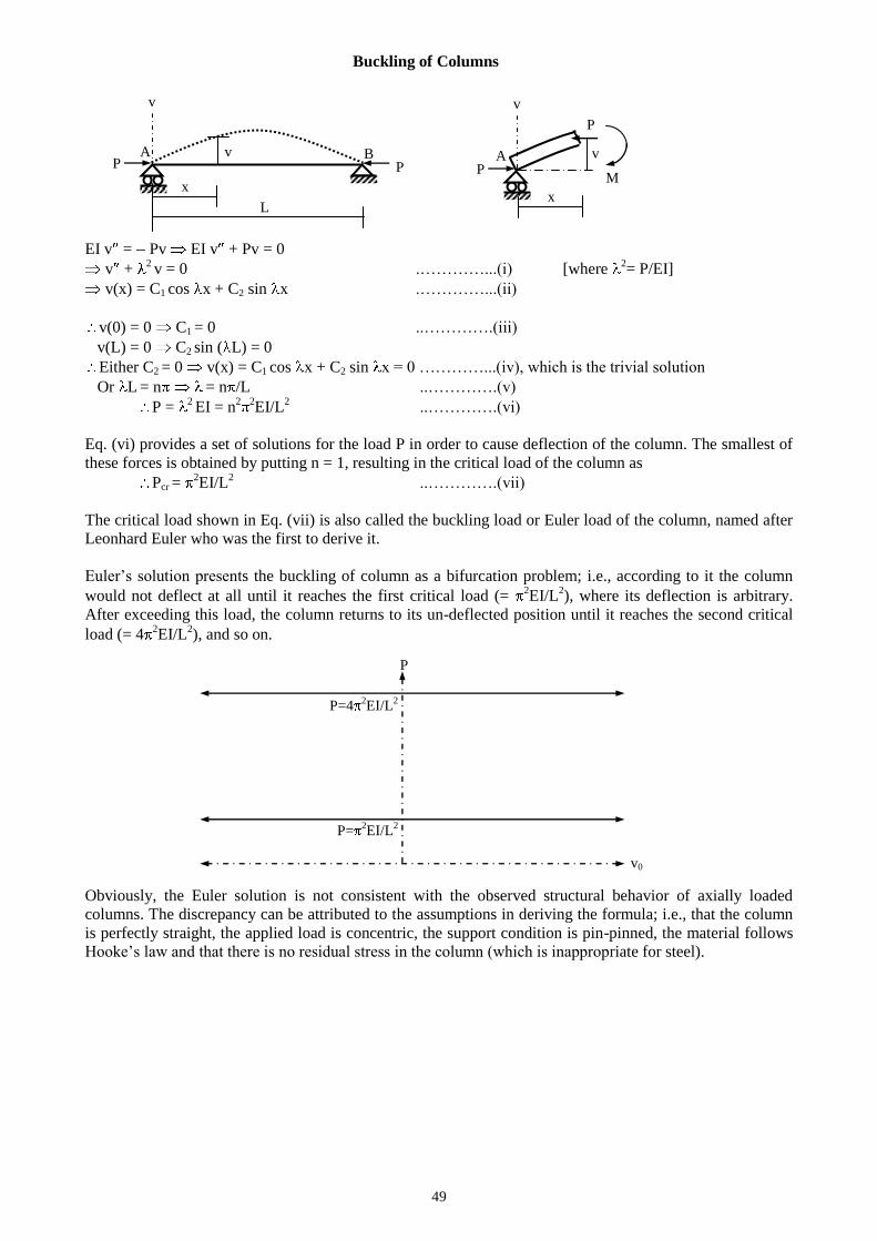
49
Buckling of Columns
EI v = Pv EI v + Pv = 0
v + 2 v = 0 .…………...(i) [where
2= P/EI]
v(x) = C1 cos x + C2 sin x .…………...(ii)
v(0) = 0 C1 = 0 ..………….(iii)
v(L) = 0 C2 sin ( L) = 0
Either C2 = 0 v(x) = C1 cos x + C2 sin x = 0 …………...(iv), which is the trivial solution
Or L = n = n /L ..………….(v)
P = 2 EI = n
2 2EI/L
2 ..………….(vi)
Eq. (vi) provides a set of solutions for the load P in order to cause deflection of the column. The smallest of
these forces is obtained by putting n = 1, resulting in the critical load of the column as
Pcr = 2EI/L
2 ..………….(vii)
The critical load shown in Eq. (vii) is also called the buckling load or Euler load of the column, named after
Leonhard Euler who was the first to derive it.
Euler’s solution presents the buckling of column as a bifurcation problem; i.e., according to it the column
would not deflect at all until it reaches the first critical load (= 2EI/L
2), where its deflection is arbitrary.
After exceeding this load, the column returns to its un-deflected position until it reaches the second critical
load (= 42EI/L
2), and so on.
Obviously, the Euler solution is not consistent with the observed structural behavior of axially loaded
columns. The discrepancy can be attributed to the assumptions in deriving the formula; i.e., that the column
is perfectly straight, the applied load is concentric, the support condition is pin-pinned, the material follows
Hooke’s law and that there is no residual stress in the column (which is inappropriate for steel).
v P
x
L
P A B
v v
x
v P
A
v0
P
P=2EI/L
2
P=42EI/L
2
P
M
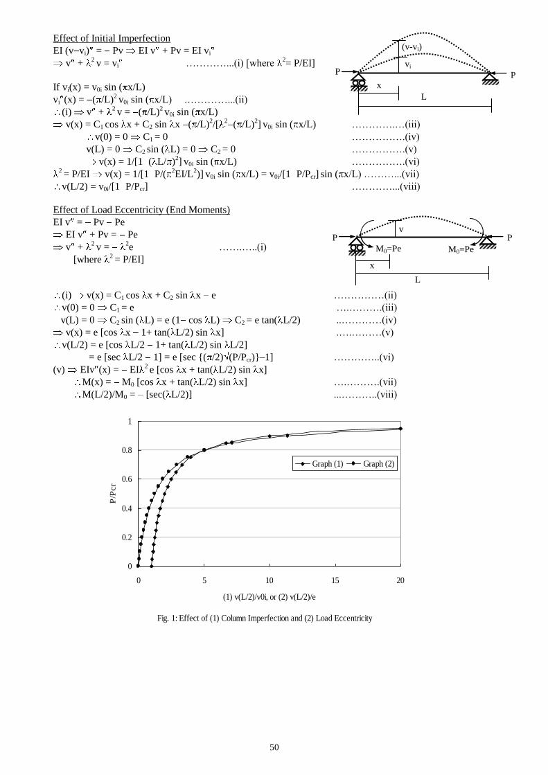
50
Effect of Initial Imperfection
EI (v vi) = Pv EI v + Pv = EI vi
v + 2 v = vi …………...(i) [where
2= P/EI]
If vi(x) = v0i sin ( x/L)
vi (x) = ( /L)2 v0i sin ( x/L) .…………...(ii)
(i) v + 2 v = ( /L)
2 v0i sin ( x/L)
v(x) = C1 cos x + C2 sin x ( /L)2/[
2( /L)
2]
v0i sin ( x/L) ………….…(iii)
v(0) = 0 C1 = 0 …………….(iv)
v(L) = 0 C2 sin ( L) = 0 C2 = 0 …………….(v)
v(x) = 1/[1 ( L/ )2]
v0i sin ( x/L) …………….(vi)
2 = P/EI v(x) = 1/[1 P/(
2EI/L
2)]
v0i sin ( x/L) = v0i/[1 P/Pcr]
sin ( x/L) ………...(vii)
v(L/2) = v0i/[1 P/Pcr] …………...(viii)
Effect of Load Eccentricity (End Moments)
EI v = Pv Pe
EI v + Pv = Pe
v + 2 v =
2e …….…..(i)
[where 2 = P/EI]
(i) v(x) = C1 cos x + C2 sin x e ……………(ii)
v(0) = 0 C1 = e ….……….(iii)
v(L) = 0 C2 sin ( L) = e (1 cos L) C2 = e tan( L/2) ..…………(iv)
v(x) = e [cos x 1+ tan( L/2) sin x] .….………(v)
v(L/2) = e [cos L/2 1+ tan( L/2) sin L/2]
= e [sec L/2 1] = e [sec {( /2) (P/Pcr)}–1] …………..(vi)
(v) EIv (x) = EI2 e [cos x + tan( L/2) sin x]
M(x) = M0 [cos x + tan( L/2) sin x] ….……….(vii)
M(L/2)/M0 = [sec( L/2)] ...………..(viii)
Fig. 1: Effect of (1) Column Imperfection and (2) Load Eccentricity
0
0.2
0.4
0.6
0.8
1
0 5 10 15 20
(1) v(L/2)/v0i, or (2) v(L/2)/e
P/P
cr
Graph (1) Graph (2)
(v-vi)
vi
P P
x
L
v P P
x
L
M0=Pe M0=Pe
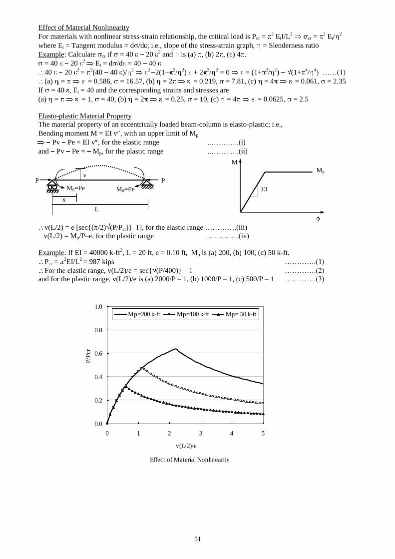
51
Effect of Material Nonlinearity
For materials with nonlinear stress-strain relationship, the critical load is Pcr = 2 EtI/L
2 cr =
2 Et/
2
where Et = Tangent modulus = d /d ; i.e., slope of the stress-strain graph, = Slenderness ratio
Example: Calculate cr if = 40 20 2 and is (a) , (b) 2 , (c) 4 .
= 40 20 2
Et = d /d = 40 40
40 20 2 =
2(40 40 )/
2
2 2(1+
2/
2) + 2
2/
2 = 0 = (1+
2/
2) (1+
4/
4) ……(1)
(a) = = 0.586, = 16.57, (b) = 2
= 0.219, = 7.81, (c) = 4
= 0.061, = 2.35
If = 40 , Et = 40 and the corresponding strains and stresses are
(a) = = 1, = 40, (b) = 2
= 0.25, = 10, (c) = 4
= 0.0625, = 2.5
Elasto-plastic Material Property
The material property of an eccentrically loaded beam-column is elasto-plastic; i.e.,
Bending moment M = EI v , with an upper limit of Mp
Pv Pe = EI v , for the elastic range ..…….…..(i)
and Pv Pe = Mp, for the plastic range ..…….…..(ii)
v(L/2) = e [sec{( /2) (P/Pcr)}–1], for the elastic range ………….(iii)
v(L/2) = Mp/P–e, for the plastic range …..……....(iv)
Example: If EI = 40000 k-ft2, L = 20 ft, e = 0.10 ft, Mp is (a) 200, (b) 100, (c) 50 k-ft.
Pcr = 2EI/L
2 = 987 kips ………….(1)
For the elastic range, v(L/2)/e = sec{ (P/400)} – 1 ………….(2)
and for the plastic range, v(L/2)/e is (a) 2000/P – 1, (b) 1000/P – 1, (c) 500/P – 1 ………….(3)
x
L
v P P
M0=Pe M0=Pe
M
Mp
EI
Effect of Material Nonlinearity
0.0
0.2
0.4
0.6
0.8
1.0
0 1 2 3 4 5
v(L/2)/e
P/P
cr
Mp=200 k-ft Mp=100 k-ft Mp= 50 k-ft
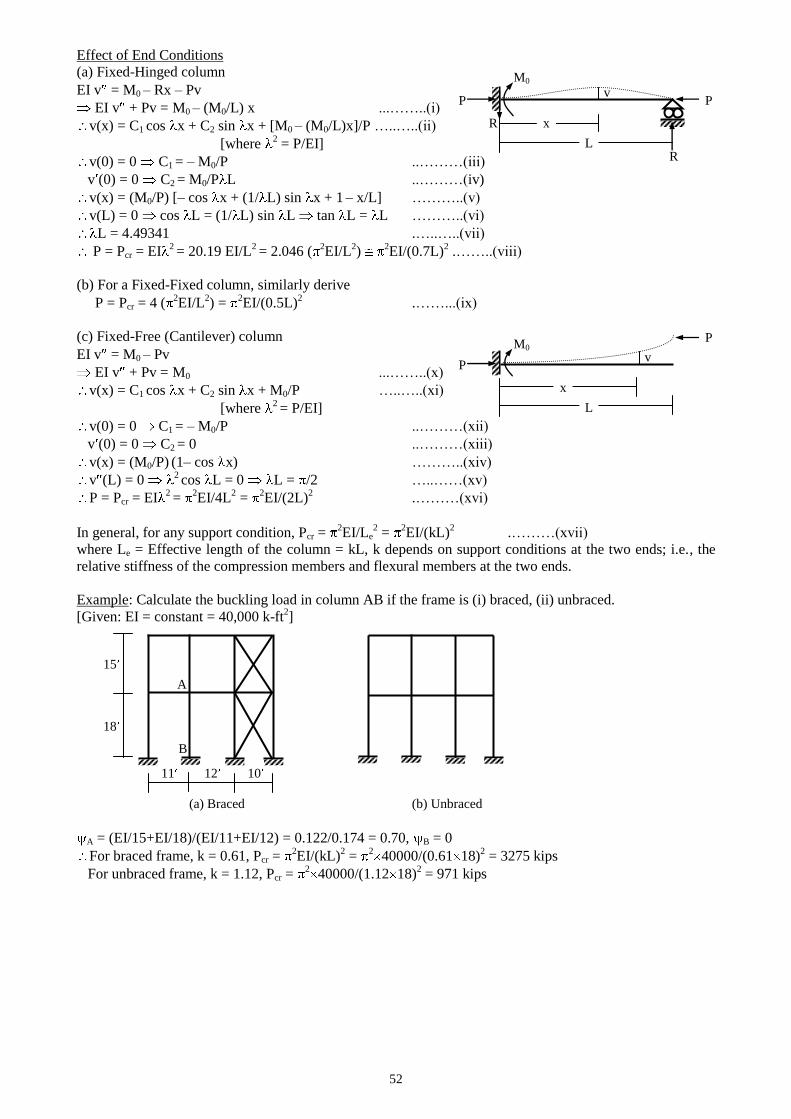
52
Effect of End Conditions
(a) Fixed-Hinged column
EI v = M0 – Rx – Pv
EI v + Pv = M0 – (M0/L) x ...……..(i)
v(x) = C1 cos x + C2 sin x + [M0 – (M0/L)x]/P …..…..(ii)
[where 2 = P/EI]
v(0) = 0 C1 = – M0/P ..………(iii)
v (0) = 0 C2 = M0/P L ..………(iv)
v(x) = (M0/P) [– cos x + (1/ L) sin x + 1 – x/L] ………..(v)
v(L) = 0 cos L = (1/ L) sin L tan L = L ………..(vi)
L = 4.49341 .…..…..(vii)
P = Pcr = EI2 = 20.19 EI/L
2 = 2.046 (
2EI/L
2)
2EI/(0.7L)
2 .……..(viii)
(b) For a Fixed-Fixed column, similarly derive
P = Pcr = 4 (2EI/L
2) =
2EI/(0.5L)
2 .……...(ix)
(c) Fixed-Free (Cantilever) column
EI v = M0 – Pv
EI v + Pv = M0 ...……..(x)
v(x) = C1 cos x + C2 sin x + M0/P …..…..(xi)
[where 2 = P/EI]
v(0) = 0 C1 = – M0/P ..………(xii)
v (0) = 0 C2 = 0 ..………(xiii)
v(x) = (M0/P) (1– cos x) ………..(xiv)
v (L) = 0 2 cos L = 0 L = /2 …..……(xv)
P = Pcr = EI2 =
2EI/4L
2 =
2EI/(2L)
2 .………(xvi)
In general, for any support condition, Pcr = 2EI/Le
2 =
2EI/(kL)
2 .………(xvii)
where Le = Effective length of the column = kL, k depends on support conditions at the two ends; i.e., the
relative stiffness of the compression members and flexural members at the two ends.
Example: Calculate the buckling load in column AB if the frame is (i) braced, (ii) unbraced.
[Given: EI = constant = 40,000 k-ft2]
15
18
11 12 10
(a) Braced (b) Unbraced
A = (EI/15+EI/18)/(EI/11+EI/12) = 0.122/0.174 = 0.70, B = 0
For braced frame, k = 0.61, Pcr = 2EI/(kL)
2 =
240000/(0.61 18)
2 = 3275 kips
For unbraced frame, k = 1.12, Pcr = 2
40000/(1.12 18)2 = 971 kips
P P
R
R
M0
L
x
v
P
P
M0
L
x
v
A
B
53
0
3.0
1.0 0.9
0.8
0.5
0.7
0.1
0.2
0.3
0.4
0.6
2.0
10.0
5.0
50.0
0
3.0
1.0 0.9
0.8
0.5
0.7
0.1
0.2
0.3
0.4
0.6
2.0
10.0
5.0
50.0
1.0
0.5
0.6
0.8
0.7
0.9
A B k
Braced Frames Unbraced Frames
Alignment Charts for Effective Length Factors k
= Ratio of EI/L of compression members to EI/L of flexural members in a plane at one end of a compression member.
k = Effective length factor.
100.0
10.0 9.0
0
20.0
7.0
6.0
5.0
1.0
2.0
3.0
4.0
8.0
30.0
50.0
100.0
10.0 9.0
0
20.0
7.0
6.0
5.0
1.0
2.0
3.0
4.0
8.0
30.0
50.0
10.0
4.0
1.0
1.5
3.0
2.0
5.0
20.0
A B k
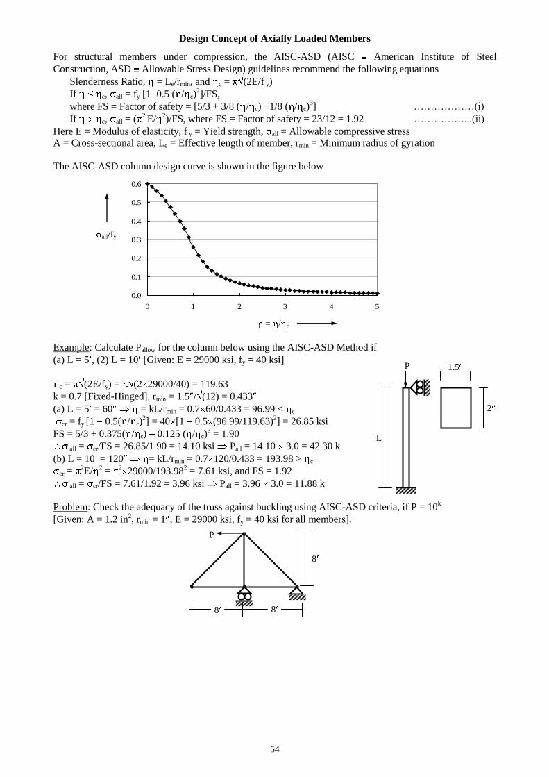
54
Design Concept of Axially Loaded Members
For structural members under compression, the AISC-ASD (AISC American Institute of Steel
Construction, ASD Allowable Stress Design) guidelines recommend the following equations
Slenderness Ratio, = Le/rmin, and c = (2E/f y)
If c, all = fy [1 0.5 ( / c)2]/FS,
where FS = Factor of safety = [5/3 + 3/8 ( / c) 1/8 ( / c)3] ………………(i)
If c, all = (2 E/
2)/FS, where FS = Factor of safety = 23/12 = 1.92 ……………...(ii)
Here E = Modulus of elasticity, f y = Yield strength, all = Allowable compressive stress
A = Cross-sectional area, Le = Effective length of member, rmin = Minimum radius of gyration
The AISC-ASD column design curve is shown in the figure below
Example: Calculate Pallow for the column below using the AISC-ASD Method if
(a) L = 5 , (2) L = 10 [Given: E = 29000 ksi, fy = 40 ksi]
c = (2E/fy) = (2 29000/40) = 119.63
k = 0.7 [Fixed-Hinged], rmin = 1.5 / (12) = 0.433
(a) L = 5 = 60 = kL/rmin = 0.7 60/0.433 = 96.99 < c
cr = fy [1 0.5( / c)2] = 40 [1 0.5 (96.99/119.63)
2] = 26.85 ksi
FS = 5/3 + 0.375( / c) 0.125 ( / c)3 = 1.90
all = cr/FS = 26.85/1.90 = 14.10 ksi Pall = 14.10 3.0 = 42.30 k
(b) L = 10 = 120 = kL/rmin = 0.7 120/0.433 = 193.98 > c
cr = 2E/
2 =
229000/193.98
2 = 7.61 ksi, and FS = 1.92
all = cr/FS = 7.61/1.92 = 3.96 ksi Pall = 3.96 3.0 = 11.88 k
Problem: Check the adequacy of the truss against buckling using AISC-ASD criteria, if P = 10k
[Given: A = 1.2 in2, rmin = 1 , E = 29000 ksi, fy = 40 ksi for all members].
L
P 1.5
2
P
8
8 8
AISC-ASD Column Design Curve
0.0
0.1
0.2
0.3
0.4
0.5
0.6
0 1 2 3 4 5
= / c
all/fy
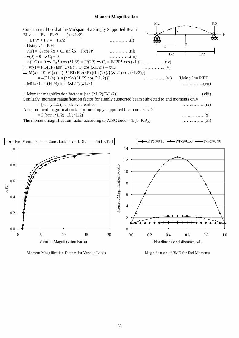
55
Moment Magnification
Concentrated Load at the Midspan of a Simply Supported Beam
EI v = Pv Fx/2 (x < L/2)
EI v + Pv = Fx/2 .………….(i)
Using 2 = P/EI
v(x) = C1 cos x + C2 sin x Fx/(2P) .………….(ii)
v(0) = 0 C1 = 0 …………..(iii)
v (L/2) = 0 C2 cos ( L/2) = F/(2P) C2 = F/(2P cos ( L)) …………….(iv)
v(x) = FL/(2P) [sin ( x)/{( L) cos ( L/2)} – x/L] ..…………...(v)
M(x) = EI v (x) = (2 EI) FL/(4P) [sin ( x)/{( L/2) cos ( L/2)}]
= (FL/4) [sin ( x)/{( L/2) cos ( L/2)}] …………….(vi) [Using 2= P/EI]
M(L/2) = (FL/4) [tan ( L/2)/( L/2)] ……..……..(vii)
Moment magnification factor = [tan ( L/2)/( L/2)] ..…..……..(viii)
Similarly, moment magnification factor for simply supported beam subjected to end moments only
= [sec ( L/2)], as derived earlier ……..……..(ix)
Also, moment magnification factor for simply supported beam under UDL
= 2 [sec ( L/2) 1]/( L/2)2 .…..……….(x)
The moment magnification factor according to AISC code = 1/(1 P/Pcr) ……..……..(xi)
v P P
x
L/2 L/2
F
F/2 F/2
Moment Magnification Factors for Various Loads
0.0
0.2
0.4
0.6
0.8
1.0
0 5 10 15 20
Moment Magnification Factor
P/P
cr
End Moments Conc. Load UDL 1/(1-P/Pcr)
Magnification of BMD for End Moments
0
2
4
6
8
10
12
14
0.0 0.2 0.4 0.6 0.8 1.0
Nondimensional distance, x/L
Mo
men
t M
ag
nif
icati
on
M/M
0
P/Pcr=0.10 P/Pcr=0.50 P/Pcr=0.90
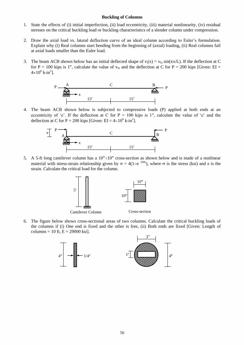
56
Buckling of Columns
1. State the effects of (i) initial imperfection, (ii) load eccentricity, (iii) material nonlinearity, (iv) residual
stresses on the critical buckling load or buckling characteristics of a slender column under compression.
2. Draw the axial load vs. lateral deflection curve of an ideal column according to Euler’s formulation.
Explain why (i) Real columns start bending from the beginning of (axial) loading, (ii) Real columns fail
at axial loads smaller than the Euler load.
3. The beam ACB shown below has an initial deflected shape of vi(x) = v0i sin( x/L). If the deflection at C
for P = 100 kips is 1 , calculate the value of v0i and the deflection at C for P = 200 kips [Given: EI =
4 106 k-in
2].
15 15
4. The beam ACB shown below is subjected to compressive loads (P) applied at both ends at an
eccentricity of ‘e’. If the deflection at C for P = 100 kips is 1 , calculate the value of ‘e’ and the
deflection at C for P = 200 kips [Given: EI = 4 106 k-in
2].
15 15
5. A 5-ft long cantilever column has a 10 10 cross-section as shown below and is made of a nonlinear
material with stress-strain relationship given by = 4(1 e100
), where is the stress (ksi) and is the
strain. Calculate the critical load for the column.
6. The figure below shows cross-sectional areas of two columns. Calculate the critical buckling loads of
the columns if (i) One end is fixed and the other is free, (ii) Both ends are fixed [Given: Length of
columns = 10 ft, E = 29000 ksi]. 3
4 1/4 4
1
Cross-section Cantilever Column
5
10
10
A C B
x
P P
A C B
x
P P e
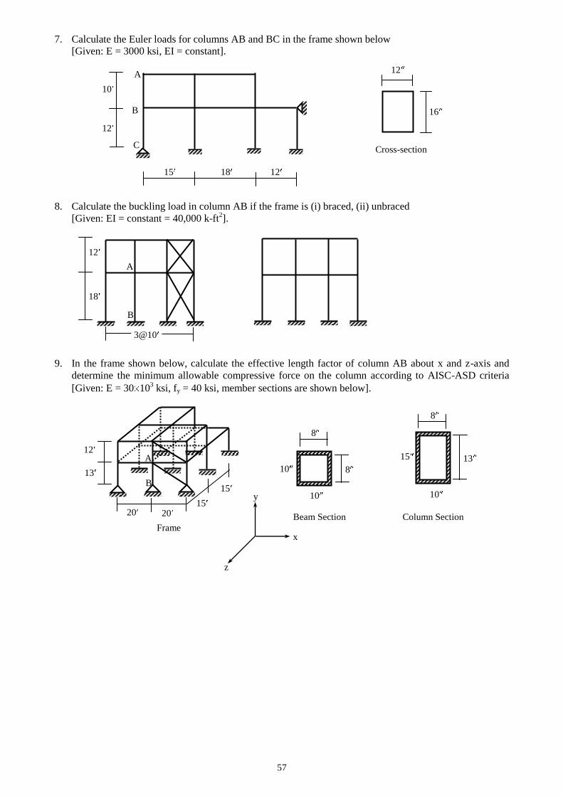
57
7. Calculate the Euler loads for columns AB and BC in the frame shown below
[Given: E = 3000 ksi, EI = constant].
15 18 12
8. Calculate the buckling load in column AB if the frame is (i) braced, (ii) unbraced
[Given: EI = constant = 40,000 k-ft2].
12
18
9. In the frame shown below, calculate the effective length factor of column AB about x and z-axis and
determine the minimum allowable compressive force on the column according to AISC-ASD criteria
[Given: E = 30 103 ksi, fy = 40 ksi, member sections are shown below].
Beam Section Column Section
Frame
B
A
3@10
A
B
20 15
20
15
13
12
10
10
10
13
8
8
8
15
x
y
z
B
C
12
16
10
12
A
Cross-section
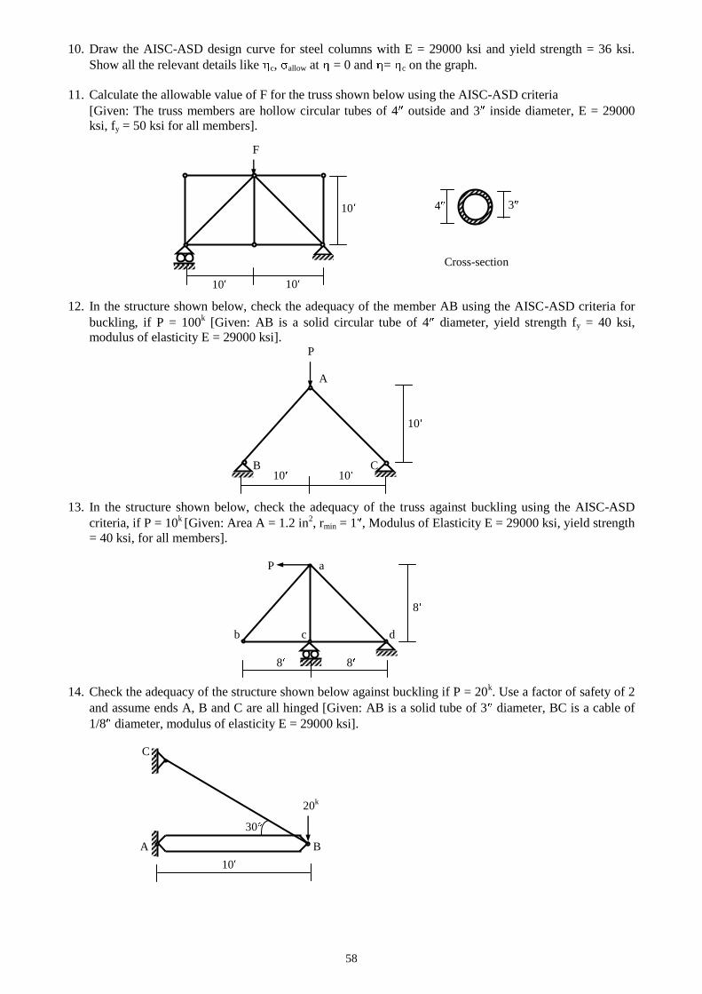
58
10. Draw the AISC-ASD design curve for steel columns with E = 29000 ksi and yield strength = 36 ksi.
Show all the relevant details like c, allow at = 0 and = c on the graph.
11. Calculate the allowable value of F for the truss shown below using the AISC-ASD criteria
[Given: The truss members are hollow circular tubes of 4 outside and 3 inside diameter, E = 29000
ksi, fy = 50 ksi for all members].
12. In the structure shown below, check the adequacy of the member AB using the AISC-ASD criteria for
buckling, if P = 100k [Given: AB is a solid circular tube of 4 diameter, yield strength fy = 40 ksi,
modulus of elasticity E = 29000 ksi]. P
A
B C
13. In the structure shown below, check the adequacy of the truss against buckling using the AISC-ASD
criteria, if P = 10k [Given: Area A = 1.2 in
2, rmin = 1 , Modulus of Elasticity E = 29000 ksi, yield strength
= 40 ksi, for all members].
P a
8
b c d
8 8
14. Check the adequacy of the structure shown below against buckling if P = 20k. Use a factor of safety of 2
and assume ends A, B and C are all hinged [Given: AB is a solid tube of 3 diameter, BC is a cable of
1/8 diameter, modulus of elasticity E = 29000 ksi].
C
20k
A B
30
10
10
10
10 10
4 3
Cross-section
10 10
F
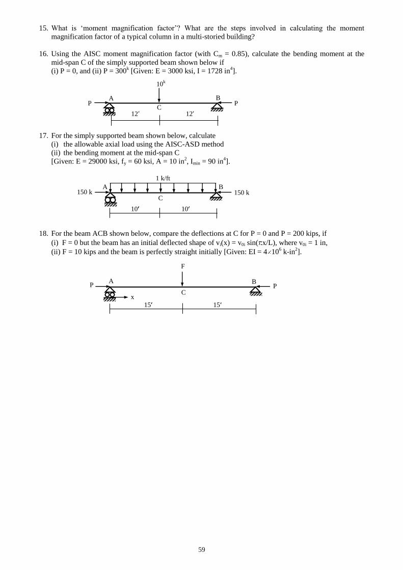
59
15. What is ‘moment magnification factor’? What are the steps involved in calculating the moment
magnification factor of a typical column in a multi-storied building?
16. Using the AISC moment magnification factor (with Cm = 0.85), calculate the bending moment at the
mid-span C of the simply supported beam shown below if
(i) P = 0, and (ii) P = 300k [Given: E = 3000 ksi, I = 1728 in
4].
P P
17. For the simply supported beam shown below, calculate
(i) the allowable axial load using the AISC-ASD method
(ii) the bending moment at the mid-span C
[Given: E = 29000 ksi, fy = 60 ksi, A = 10 in2, Imin = 90 in
4].
10 10
18. For the beam ACB shown below, compare the deflections at C for P = 0 and P = 200 kips, if
(i) F = 0 but the beam has an initial deflected shape of vi(x) = v0i sin( x/L), where v0i = 1 in,
(ii) F = 10 kips and the beam is perfectly straight initially [Given: EI = 4 106 k-in
2].
15 15
C
B A
10k
F
A
C
B
x
P P
12 12
A B
C
1 k/ft
150 k 150 k
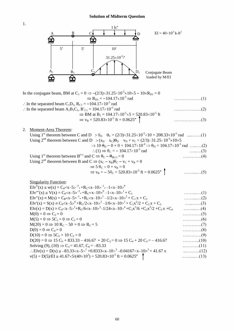
60
Solution of Midterm Question
1.
5 5 10
In the conjugate beam, BM at C1 = 0 (2/3) 31.25 10-5
10 5 10 RD1 = 0
RD1 = 104.17 10-5
rad ……………….(1)
In the separated beam C1D1, RC1 = 104.17 10-5
rad
In the separated beam A1B1C1, R C1 = 104.17 10-5
rad ……………….(2)
BM at B1 = 104.17 10-5
5 = 520.83 10-5
ft
vB = 520.83 10-5
ft = 0.0625 ……………….(3)
2. Moment-Area Theorem:
Using 1st theorem between C and D D C = (2/3) 31.25 10
-510 = 208.33 10
-5 rad .....……(1)
Using 2nd
theorem between C and D (xD xC) D vD + vC = (2/3) 31.25 10-5
10 5
10 D 0 + 0 = 104.17 10-4
D = 104.17 10-5
rad …..….(2)
(1) C = 104.17 10-5
rad …..….(3)
Using 1st theorem between B
(+) and C C B(+) = 0 ………….(4)
Using 2nd
theorem between B and C (xC xB) C vC + vB = 0
5 C 0 + vB = 0
vB = 5 C = 520.83 10-5
ft = 0.0625 ……....…(5)
Singularity Function:
EIviv(x) w(x) = C x–5
–3* +RC x–10
–1* –1 x–10
0
EIv (x) V(x) = C x–5–2
* +RC x–10
0 –1 x–10
1 + C1 ……....…(1)
EIv (x) M(x) = C x–5–1
* +RC x–10
1 –1/2 x–10
2 + C1 x + C2 ……....…(2)
EIv (x) = S(x) C x–50 +RC/2 x–10
2 –1/6 x–10
3 + C1x
2/2 + C2 x + C3 …...……(3)
EIv(x) = D(x) C x–51+RC/6 x–10
3–1/24 x–10
4 +C1x
3/6 +C2x
2/2 +C3 x +C4 ……....…(4)
M(0) = 0 C2 = 0 ………….(5)
M(5) = 0 5C1 = 0 C1 = 0 ………….(6)
M(20) = 0 10 RC – 50 = 0 RC = 5 ………….(7)
D(0) = 0 C4 = 0 ………….(8)
D(10) = 0 5C + 10 C3 = 0 ………….(9)
D(20) = 0 15 C + 833.33 – 416.67 + 20 C3 = 0 15 C + 20 C3 = – 416.67 ………...(10)
Solving (9), (10) C3 = 41.67, C = –83.33 ..……….(11)
EIv(x) = D(x) –83.33 x–51 +0.8333 x–10
3 –0.04167 x–10
3 + 41.67 x ..……….(12)
v(5) = D(5)/EI 41.67 5/(40 103) = 520.83 10
-5 ft = 0.0625 ……....…(13)
EI = 40 103 k-ft
2
1 k/
A C D B
31.25 10-5
/
A1 C1 D1 B1 Conjugate Beam
loaded by M/EI
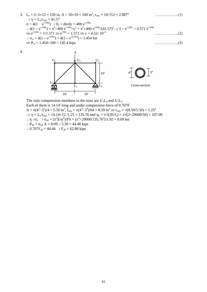
61
3. Le = 2 5 12 = 120 in, A = 10 10 = 100 in2, rmin = 10/ 12 = 2.887 ………………(1)
= Le/rmin = 41.57
= 4(1 e100
)
Et = d /d = 400 e100
4(1 e100
) = 2
400 e100
/2 =
2400 e
100/(41.57)
2 1 e
100 = 0.571 e
100
e100
= 1/1.571 e100
= 1.571 = 4.52 103 ………………(2)
cr = 4(1 e100
) = 4(1 e0.452
) = 1.454 ksi
Pcr = 1.454 100 = 145.4 kips ………………(3)
4.
The only compression members in the truss are U1L0 and U1L2
Each of them is 14.14 long and under compressive force of 0.707F
A = (42
32)/4 = 5.50 in
2, Imin = (4
43
4)/64 = 8.59 in
4 rmin = (8.59/5.50) = 1.25
= Le/rmin = 14.14 12 /1.25 = 135.76 and c = (2E/fy) = (2 29000/50) = 107.00
c all = (2E/
2)/FS = (
229000/135.76
2)/1.92 = 8.09 ksi
Pall = all A = 8.09 5.50 = 44.46 kips
0.707Fall = 44.46 Fall = 62.88 kips
F
10
10 10
4 3
Cross-section
U0 U1 U2
L0 L1 L2