tossing coin game and linear programming big_m simplex algorithms duc nguyen, old dominion...

Tossing Coin Game and Linear Programming Big_M Simplex

Algorithms

Duc Nguyen , Old Dominion University, USAYuzhong Shen , Old Dominion University, USA

Ahmed Ali Mohammed , Old Dominion University, USASubhash Chandra Bose Kadiam , Old Dominion University,

USA

IntroductionLinear Programming (LP) is a very popular/important topic, with very broad/real-world Engineering/Economic, and Social Science applications. In addition to Operation Research, LP course has been offered in most (if not all) engineering curriculum in the USA.

Teaching LP topic, however, may not be an easy task, especially at the undergraduate, and/or even at the high-school levels. Through simple Head-Tail (Tossing Coin) game strategies, and coupling with graphical and Simplex methods, the authors hope that the formulation and optimal solution for LP problem can be easily understood even by high-school students.

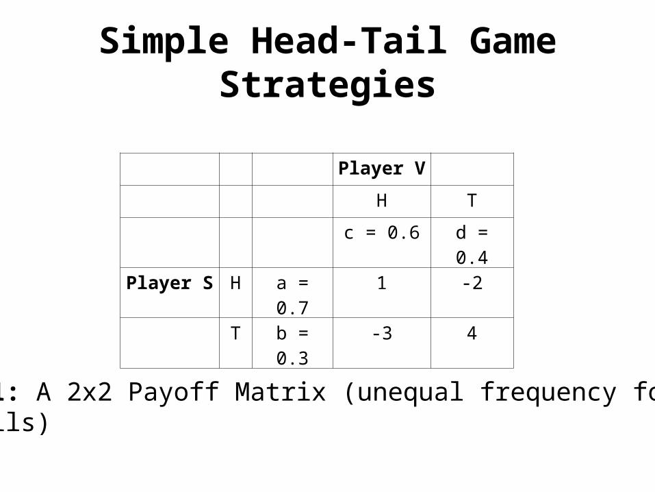
Player V

H T

c = 0.6 d = 0.4

Player S H a = 0.7 1 -2

T b = 0.3 -3 4

Table 1: A 2x2 Payoff Matrix (unequal frequency for Heads and Tails)

Simple Head-Tail Game Strategies


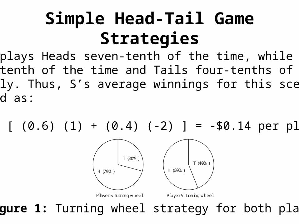
Step 1. S plays Heads seven-tenth of the time, while V plays Heads six-tenth of the time and Tails four-tenths of the time respectively. Thus, S’s average winnings for this scenario can be computed as:

S1 = (0.7) [ (0.6) (1) + (0.4) (-2) ] = -$0.14 per play

T (30%)

H (70%)

Player S turning wheel

T (40%)

H (60%)

Player V turning wheel

Figure 1: Turning wheel strategy for both players.

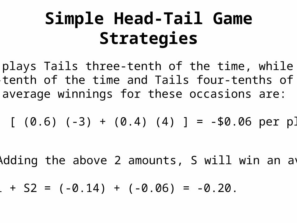
Step 2. S plays Tails three-tenth of the time, while V plays Heads six-tenth of the time and Tails four-tenths of the time. Thus, S’s average winnings for these occasions are:

S2 = (0.3) [ (0.6) (-3) + (0.4) (4) ] = -$0.06 per play

Step 3. Adding the above 2 amounts, S will win an average of:

Stotal = S1 + S2 = (-0.14) + (-0.06) = -0.20.


Game-Based Linear Programming (LP) Optimization Formulation

Consider “V’s ≡ Victoria’s” strategies (c,d), such that

0;0 dc

1 dc

In the above Eqs. (1-2), “c” and “d” represents the desired/selected probability for V to observe HEAD and TAIL, respectively.

(1)

(2)

V expect to lose over S’s two pure strategies (1,0), and (0,1), respectively by the following amounts:

dcdc 21)]4)(0()2)(1[()]3)(0()1)(1[(

dcdc 43)]4)(1()2)(0[()]3)(1()1)(0[(

(3)

(4)


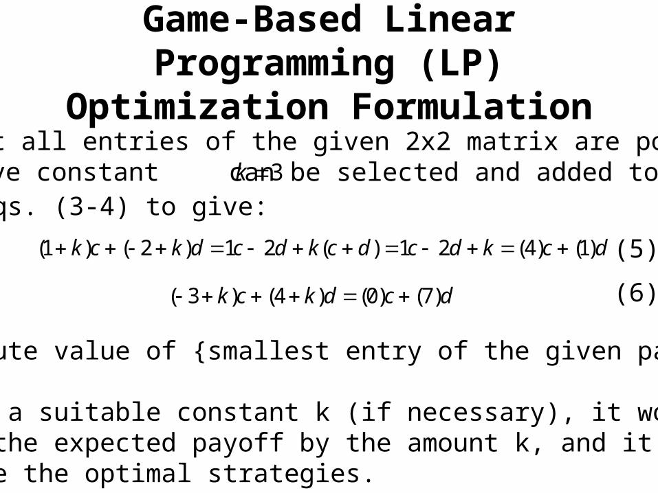
Since not all entries of the given 2x2 matrix are positive, a positive constant can be selected and added to3k

dckdcdckdcdkck )1()4(21)(21)2()1(

dcdkck )7()0()4()3( Notes:k = absolute value of {smallest entry of the given payoff matrix}By adding a suitable constant k (if necessary), it would simply increase the expected payoff by the amount k, and it would NOT change the optimal strategies.

Eqs. (3-4) to give:

(5)

(6)


Define:= maximum (4c+1d, 0c+7d)

= worse case for V

w

Then:wdc )1()4(

wdc )7()0(

(8)

(9)

(7)


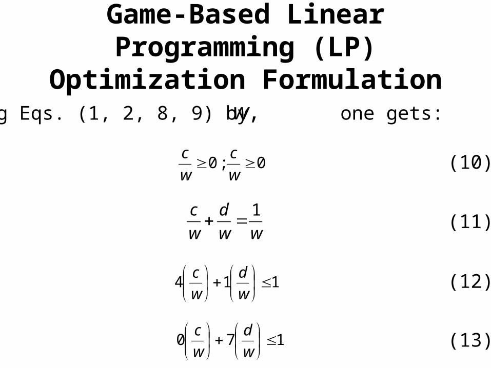
Dividing Eqs. (1, 2, 8, 9) by one gets:,w

0;0 w

c

w

c

ww

d

w

c 1

114

w

d

w

c

170

w

d

w

c

(11)

(12)

(13)

(10)


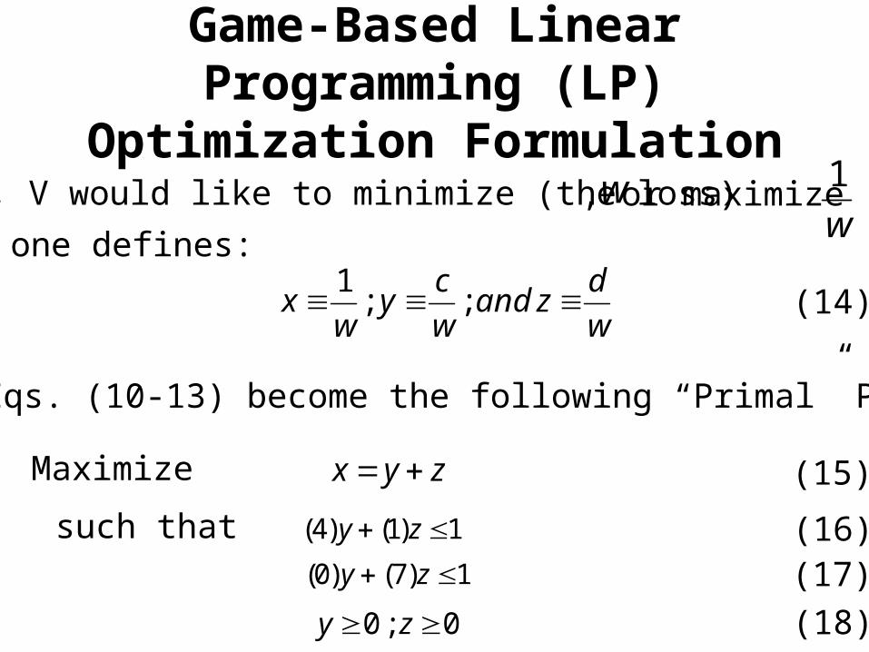
Since, V would like to minimize (the loss) w, or maximize w

1

one defines:

w

dzand

w

cy

wx ;;

1

Then, Eqs. (10-13) become the following “Primal” Problem:

Maximize zyx

such that 1)1()4( zy

1)7()0( zy

0;0 zy

(15)

(16)(17)(18)

(14)


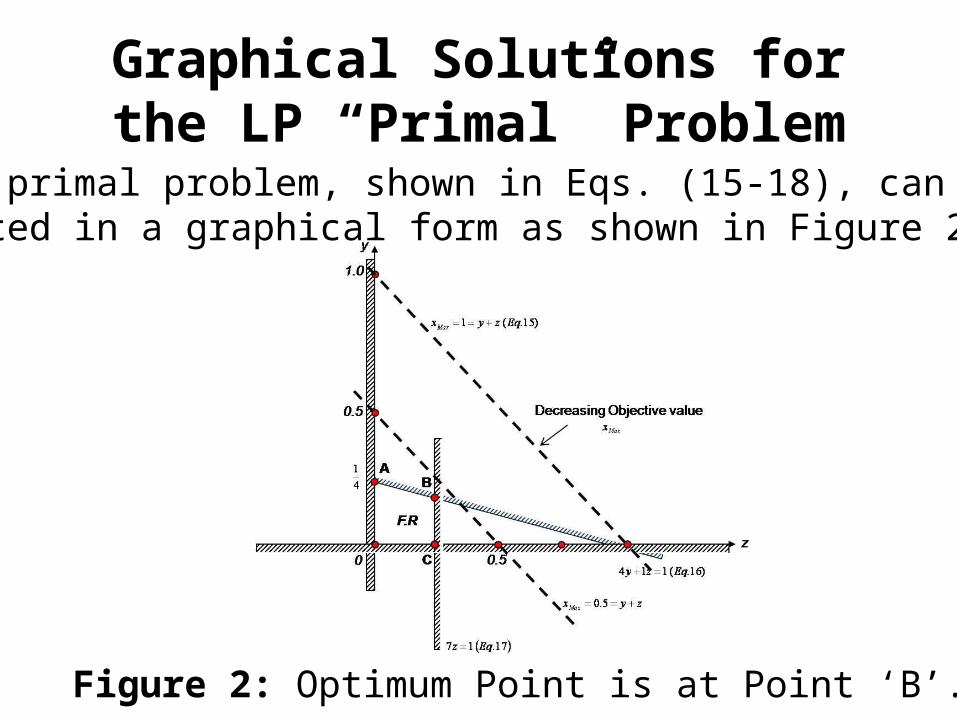
Graphical Solutions for the LP “Primal” Problem

The LP primal problem, shown in Eqs. (15-18), can be presented in a graphical form as shown in Figure 2

Figure 2: Optimum Point is at Point ‘B’.

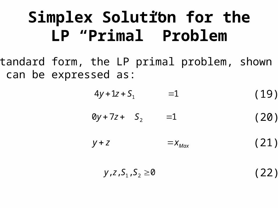
Simplex Solution for the LP “Primal” Problem

In the standard form, the LP primal problem, shown in Eqs. (15-18), can be expressed as:

114 1 Szy

170 2 Szy

Maxxzy

0,,, 21 SSzy

(19)

(20)

(21)

(22)

For the above standard LP problem, one has 2 (equality) constraints (see Eqs. 19-20) and

and non-basic variables4 unknown variables

Non-basic variables, by definitions, will have “Zero” numerical values. Basic variables, therefore, are the ones which have “canonical forms” (The column under each BASIC variable should have all entries to be 0, except only one entry to be equal to 1, as can be observed in Figure 3) and have their numerical values to be equal to the Right-Hand-Side (RHS) values of constraint equations (19-20).

21 , SS )., zy(basic variables


The basic/popular Simplex Algorithms [2,5] are based on the following main ideas:

1. In each iteration, we have to decide which non-basic variable will be selected to ENTER into the basic variable group?, and

2. Which basic variable will be KICKED OUT from the basic variable group?3. The objective function (see Eq. 21) should always be expressed in terms of “non-basic variables” to satisfy the “canonical form” requirement.4. The iterative process will be stopped if no further improvements can be done.


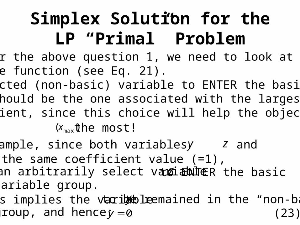
To answer the above question 1, we need to look at the objective function (see Eq. 21). The selected (non-basic) variable to ENTER the basic variable group should be the one associated with the largest positive coefficient, since this choice will help the objective function )( maxx the most!In this example, since both variables and have the same coefficient value (=1), we can arbitrarily select variable to ENTER the basic

This implies the variable to be remained in the “non-basic”0y

y z

z

yvariable group.

group, and hence: (23)


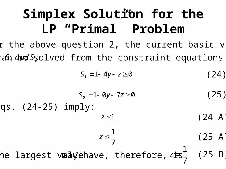
To answer the above question 2, the current basic variables

21 SandS can be solved from the constraint equations (19-20):

0411 zyS

07012 zyS

Eqs. (24-25) imply:1z

7

1z

The largest value may have, therefore, is z7

1z

(24 A)

(25 B)

(25 A)

(24)

(25)


7

6

7

111

zS

07

1712

zS

02 S

2S

Comparing Eqs. (26-27), since , hence the basic variable should be one to be kicked out from the basic group (or

entering into the non-basic group)!

(26)

(27)


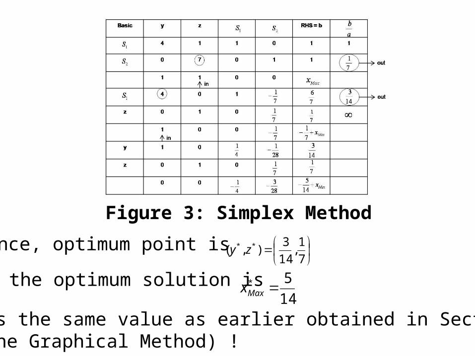
Figure 3: Simplex Method

Hence, optimum point is

and the optimum solution is

which has the same value as earlier obtained in Section 4 (using the Graphical Method) !

7

1,

14

3),( ** zy

14

5* Maxx

BIG_M Simplex Solution Method [2,5]Artificial variables are “NOT” required in the above LP problem, since it only involves “<” type constraints. However, for those LP problems that have “>, or =” type constraints, then artificial variables need be introduced (in order to have proper canonical form, and to have the starting SIMPLEX iteration !). for convenience, let’s introduce artificial variables into the 2 constraint Eqs. (19-20), 1A 2Aand

114 11 ASzy

170 22 ASzyand

max_)()( 21 xAAMzy

and the objective function Eq. (21), respectively. Then, the following Big_M SIMPLEX LP problem can be formulated:

(28)

(29)

(30)

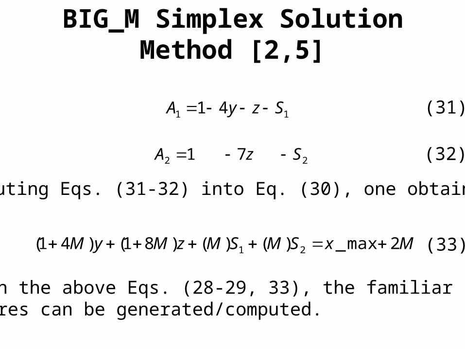
11 41 SzyA

22 71 SzA

Substituting Eqs. (31-32) into Eq. (30), one obtains:

MxSMSMzMyM 2max_)()()81()41( 21

Based on the above Eqs. (28-29, 33), the familiar SIMPLEX procedures can be generated/computed.

(31)

(32)

(33)

BIG_M Simplex Solution Method [2,5]

Real-World “Racial Desegregation of School/Bus Systems” Application

[2,4]Since the landmark Supreme Court decision in 1954 invalidating school segregation, the problem of racial desegregation of school systems has received a great deal of attention.

In urban communities, where residential patterns produce de facto segregation of schools, many school administrations have adopted an official policy of eliminating such segregation by busing students (or else face the loss of federal funds).

The following (collected) data are given:

Using the above given data, and the Simplex algorithm explained in Section 6, undergraduate students will be able to formulate the LP problem, and find the “optimum” solution which

1. Places each student in a school.2. Achieves an ethnic composition within the given ranges for each school.3. Minimizes the total daily student transportation time (or any other objective that one might consider pertinent).

Distributions of Ethnic Groups (A, B, C), School Districts (1, 2, 3), and Students Populations. Schools’ (I, II, III, IV) Capacities. Allowable (minimum %, maximum %) Ethnic Groups’ Composition. Travel Time between Districts (1, 2, 3) and Schools (I, II, III, IV).

AcknowledgementsThe authors would like to acknowledge the partial support, provided in this work through the National Science Foundation (NSF Grant #0836916).

www.brothersoft.com/downloads/flash-animation-software.html

References

D. Belegundu, and T. R. Chandrupatla. (1999). Optimization Concepts and Applications in Engineering, Prentice-Hall Publishers.

P.A. Steenbrink. (1974). Optimization of Transport Networks. John Wiley & Sons Publisher.

Duc T. Nguyen. (2006). Finite Element Methods: Parallel-Sparse Statics and Eigen-Solutions, Springer Publishers.

Duc T. Nguyen, Cee-715/815: Engineering Optimization I; http://www.lions.odu.edu/~skadi002

tossing coin game and linear programming big_m simplex algorithms duc nguyen, old dominion...

Documents