total maximum daily load for pathogens in san luis obispo ......total maximum daily load for...
TRANSCRIPT
Resolution No. R3-2004-0142 Attachment B December 3, 2004
Phase Six: Regulatory Action Selection
Final Project Report
Total Maximum Daily Load for Pathogens in San Luis Obispo
Creek, San Luis Obispo County, California
October 2004
Central Coast Regional Water Quality Control Board 895 Aerovista Place, Suite 101 San Luis Obispo, CA 93401
Contact:
Christopher Rose 805-542-4770

Resolution No. R3-2004-0142 Attachment B December 3, 2004
CONTENTS Contents ............................................................................................................................... i Tables................................................................................................................................. iii Figures................................................................................................................................ iv 1. Project Definition........................................................................................................ 1
1.1. Beneficial Uses ................................................................................................... 1 1.2. Problem Statement .............................................................................................. 4 1.3. Accompanying Spreadsheet Containing Data and Analysis............................... 4
2. Watershed Description................................................................................................ 5 2.1. Location, Climate, and Hydrology...................................................................... 5 2.2. Land-Uses ........................................................................................................... 8
3. Data Analysis ............................................................................................................ 11 3.1. Water Quality Data ........................................................................................... 11 3.2. Flow Data.......................................................................................................... 15 3.3. DNA Fingerprinting.......................................................................................... 15 3.4. Data Analysis Summary ................................................................................... 16
4. Source Analysis ........................................................................................................ 18 4.1. Approach........................................................................................................... 18
Approach Inherently Conservative ........................................................................... 20 Individual Calculations ............................................................................................. 20
4.2. Source Categories ............................................................................................. 20 4.3. Sources Contributing to Monitoring Site 10.0.................................................. 21
Sources in Stenner Creek Watershed........................................................................ 22 Sources from Upper Stenner and Lower Stenner Creek Watershed..................... 23 Sources from Brizzolara Creek Watershed........................................................... 24 Sources from Garden Creek Watershed................................................................ 24
San Luis Obispo Creek Main Stem Sources to Site 10.0.......................................... 25 Sources from Upper and Reservoir and Portions of Upper City Watersheds....... 26 Sources from the Tunnel....................................................................................... 27
4.4. Summary of Source Analysis............................................................................ 30 4.5. Point and Non-Point Sources ............................................................................ 35
Point Sources ............................................................................................................ 35 Non-Point Sources .................................................................................................... 35
5. Critical Conditions and Seasonal Variation.............................................................. 36 6. Numeric Target ......................................................................................................... 38 7. Linkage Analysis ...................................................................................................... 40 8. TMDL Calculation and Allocations.......................................................................... 41
8.1. Allocations ........................................................................................................ 41 8.2. Wasteload Allocations ...................................................................................... 44 8.3. Load Allocations............................................................................................... 44 8.4. Margin of Safety ............................................................................................... 44
Low-flow Data Collection ........................................................................................ 44 Assumption of Zero Die-off and Predation .............................................................. 45
9. Public Participation................................................................................................... 47
Resolution No. R3-2004-0142 Attachment B December 3, 2004 10. Implementation Plan ............................................................................................. 48
10.1. Introduction................................................................................................... 48 10.2. Required Trackable Implementation Actions ............................................... 48 10.3. Responsibilities of Regional Board .............................................................. 51
Executive Officer or Regional Board Amends Monitoring and Reporting and Storm Water Management Requirements............................................................................ 51 Regional Board Assessment ..................................................................................... 51
10.4. Timeline and Milestones............................................................................... 51 10.5. Existing Efforts to Reduce Coliform Levels................................................. 52 10.6. Cost-estimate of Implementation.................................................................. 52
11. Monitoring Plan .................................................................................................... 54 11.1. Introduction................................................................................................... 54 11.2. Monitoring Sites, Frequency, and Responsible Parties ................................ 54 11.3. Reporting....................................................................................................... 56
References......................................................................................................................... 57 Appendix A: data .............................................................................................................. 59 Appendix B: Example Calculations.................................................................................. 68

Resolution No. R3-2004-0142 Attachment B December 3, 2004
TABLES Table 2.1 Land-use Areas in San Luis Obispo Creek Watershed....................................... 9 Table 4.1 Land-uses in Stenner Creek Watersheds .......................................................... 22 Table 4.2 Land-uses Contributing Flow to Site 10.0 ........................................................ 25 Table 4.3 Relative Source Contributions to Coliform Concentration in Stenner Cr. ....... 31 Table 4.4 Relative Contributions to Coliform Concentration in Main Stem upstream of
confluence with Stenner Cr....................................................................................... 32 Table 4.5 Relative Contributions to Coliform Concentration in San Luis Obispo Creek. 33 Table 8.1 Geographically-referenced Allocations ............................................................ 43 Table 10.1 Schedule and Trackable Implementation Actions of Responsible Dischargers
................................................................................................................................... 49 Table 10.2 Annual Cost Estimate of Implementation....................................................... 53 Table 11.1 Creek monitoring, responsible parties, sites, frequency, and constituent....... 55

Resolution No. R3-2004-0142 Attachment B December 3, 2004
FIGURES Figure 1.1 Log Mean of Fecal Coliform Concentration of 5 Samples ............................... 3 Figure 2.1 Location of San Luis Obispo Creek Watershed ................................................ 6 Figure 2.2 San Luis Obispo Creek Watershed.................................................................... 7 Figure 2.3 Land-use in San Luis Obispo Creek Watershed.............................................. 10 Figure 3.1 Monitoring Sites along Main Stem of Creek................................................... 12 Figure 3.2 Monitoring Sites Along Tributaries................................................................. 13 Figure 3.3 San Luis Obispo Creek Fecal Coliform Concentration Over Time ................ 14 Figure 3.4 San Luis Obispo Creek Flow During Summer 2002....................................... 15 Figure 4.1 Watershed area draining to site 10.0 ............................................................... 21 Figure 4.2 Monitoring Sites in Stenner Creek Watershed ................................................ 23 Figure 4.3 Main Stem Monitoring Sites in Downtown Area............................................ 26 Figure 4.4 Median Fecal Coliform Values Upstream and Downstream from Tunnel...... 27 Figure 4.5 DNA identified sources of E. coli in tunnel. ................................................... 28 Figure 4.6 Relative Contributions by Sources to Fecal Coliform Concentration in San
Luis Obispo Cr.......................................................................................................... 34 Figure 5.1 Seasonal Coliform Concentrations .................................................................. 37 Figure 8.1 Allocation Reference Points ............................................................................ 42 Figure 8.2 Fecal Coliform Concentration Plotted Against Observed Flow at Site 10.3... 45 Figure 11.1 Locations of Monitoring Sites ....................................................................... 55

TMDL for Pathogens in San Luis Obispo Creek August, 2004
1. PROJECT DEFINITION This document addresses impairment of San Luis Obispo Creek by pathogens due to its placement on the 303(d) list for impaired waterbodies. This document further calculates a Total Maximum Daily Load (TMDL) for fecal coliform for San Luis Obispo Creek, located in San Luis Obispo County, California. San Luis Obispo Creek (Creek) was placed on the 303(d) list for pathogens in 1996. The listing was prompted by data indicating that fecal coliform bacteria levels exceeded Basin Plan objectives for the protection of water contact recreation. Data used to support the listing were gathered from the lower reaches of the Creek, resulting in a listing for the lower nine of seventeen miles of the main stem. Funding for the project was acquired in 2001. Consequently, monitoring efforts commenced in March 2001. Water quality analysis focused on fecal and total coliform. Fecal coliform are used as an indicator organism for the presence of pathogenic organisms. In addition, some beneficial uses are protected through Water Quality Control Plan objectives utilizing fecal coliform concentration.
1.1. Beneficial Uses
The Water Quality Control Plan for the Central Coast Region (Basin Plan) identifies the following thirteen beneficial uses of the Creek and its tributaries. − Municipal and Domestic Water Supply (MUN) − Agricultural Supply (AGR) − Ground Water Recharge (GWR) − Water Contact Recreation (REC-1) − Non-Contact Water Recreation (REC-2) − Wildlife Habitat (WILD) − Cold Freshwater Habitat (COLD) − Warm Freshwater Habitat (WARM) − Migration of Aquatic Organisms (MIGR) − Spawning, Reproduction, and/or Early Developments (SPWN) − Rare, Threatened, or Endangered Species (RARE) − Freshwater Replenishment (FRSH) − Commercial and Sport Fishing (COMM) In addition to the beneficial uses above, the Creek is also designated to support Shellfish harvesting (SHELL) and Aquaculture (AQUA) at the mouth of the Creek. Of the beneficial uses outlined above, REC-1 and SHELL are protected by the most stringent water quality objectives protecting against pathogenic organisms. Fecal and total coliform concentrations are used as indicators for the presence of pathogens. The water quality objective for the protection of REC-1 is stated as follows:
1

TMDL for Pathogens in San Luis Obispo Creek August, 2004
“Fecal coliform concentration, based on a minimum of not less than five samples for any 30-day period, shall not exceed a log mean of 200/100 mL, nor shall more than ten percent of the total samples during any 30-day period exceed 400/100 mL.” (Water Quality Control Plan, Central Coast Region)
•
•
The water quality objective for the protection of SHELL is stated as follows:
“At all areas where shellfish may be harvested for human consumption, the median total coliform concentration throughout the water column for any 30-day period shall not exceed 70/100 mL, nor shall more than ten percent of the samples collected during any 30-day period exceed 230/100 mL for a five-tube decimal dilution test or 330/100 mL when a three-tube decimal dilution test is used.” (Water Quality Control Plan, Central Coast Region).
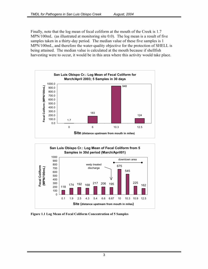
These water quality objectives are used as a gauge to confirm the listing of the Creek as impaired due to pathogens and further help staff determine where problem locations exist. The problem statement, contained in this section, summarizes key data in this determination. Regional Water Quality Control Board staff (staff) began collecting water column samples in March 2001. Sampling ended in April 2003. The sampling began with the collection of 5 samples in the 30-day period at eleven locations along the main stem of the Creek. Five of the eleven monitoring points carried fecal coliform log-means exceeding the water quality objective of 200 MPN/100 mL for the protection of REC-1. Five samples were collected in a 30-day period in March and April of 2003 at four locations. Of the four locations sampled, one carried a fecal coliform log mean exceeding the water quality objective for the protection of REC-1. The median total coliform level at the mouth of the Creek in March and April 2003 was less than 2 MPN/100mL, and therefore meets the water quality objective of 70 MPN/100 mL for the protection of SHELL. Figure 1.1 below summarizes results of these two monitoring efforts in the Creek (please refer to Figure 3.1 on page 12 for site locations). Note that data will be discussed in more detail in the Source Analysis section. Note from the figures that coliform concentration is elevated in the downtown area of the City. Monitoring sites 10.0 and 10.3 mark the central portion of the City and convey stream flow from several urban sources (to be discussed in the Source Analysis section). Monitoring site 10.3 is situated in the downtown area with public access to the Creek; cobbled sidewalks leading to the streams edge, as well as boulders in the Creek, have been placed to provide easy access for residents and tourists. It is this site that often carries the highest concentration of coliform. Fecal coliform concentration is significantly lower at sites 6.67 and 6.6, relative to sites 10.0 and 10.3. Monitoring sites 6.67 and 6.6 are adjacent to the discharge of the City’s wastewater treatment plant (WWTP). The WWTP discharges tertiary treated wastewater to the Creek, carrying a total coliform concentration consistently less than 3 MPN/100mL.
2
TMDL for Pathogens in San Luis Obispo Creek August, 2004
Finally, note that the log mean of fecal coliform at the mouth of the Creek is 1.7 MPN/100mL (as illustrated at monitoring site 0.0). The log mean is a result of five samples taken in a thirty-day period. The median value of these five samples is 1 MPN/100mL, and therefore the water-quality objective for the protection of SHELL is being attained. The median value is calculated at the mouth because if shellfish harvesting were to occur, it would be in this area where this activity would take place.
San Luis Obispo Cr.: Log Mean of Fecal Coliform for March/April 2003; 5 Samples in 30 days
1.7
183124
948
0.0100.0200.0300.0400.0500.0600.0700.0800.0900.0
1000.0
0 6 10.3 12.5
Site (distance upstream from mouth in miles)
Feca
l Col
iform
(MPN
/100
mL)
San Luis Obispo Cr.: Log Mean of Fecal Coliform from 5 Samples in 30d period (March/April01)
118174 192 168 217 206 195
675545
225162
0100200300400500600700800900
1000
0.1 1.9 2.5 4.3 5.4 6.6 6.67 10 10.3 10.9 12.5
Site (distance upstream from mouth in miles)
Feca
l Col
iform
(M
PN/1
00m
L)
downtown area
wwtp treated discharge
Figure 1.1 Log Mean of Fecal Coliform Concentration of 5 Samples
3

TMDL for Pathogens in San Luis Obispo Creek August, 2004
1.2. Problem Statement Fecal coliform concentration in San Luis Obispo Creek exceeds the water quality objective for the protection of REC-1 (water contact recreation). The water quality objective for the protection of REC-1 is exceeded at a location where water contact recreation occurs frequently. Consequently, fecal coliform load reduction is necessary, which in turn warrants calculation of the load reduction necessary to meet water quality objectives and a plan to achieve the necessary load reductions.
1.3. Accompanying Spreadsheet Containing Data and Analysis The spreadsheet accompanying this document contains data, calculations, and analysis used in the TMDL. Individual worksheets are titled in such a way to make their contents self-evident. Note that many of the cell formulas are linked to other cells as well as other worksheets within the spreadsheet.
4

TMDL for Pathogens in San Luis Obispo Creek August, 2004
2. WATERSHED DESCRIPTION
2.1. Location, Climate, and Hydrology The San Luis Obispo Creek Watershed (the Watershed) is located on the Central Coast of California approximately 240 miles south of San Francisco and 200 miles north of Los Angeles, as shown in Figure 2.1. The Watershed encompasses 219 km2 (84.6 mi2, 54,142 acres) and is home to the 45,000 residents of the city of San Luis Obispo (City). The City encompasses 23 km2 (9 mi2) and lies nearly in the middle of the watershed, with San Luis Obispo Creek flowing through the downtown area. The main stem of the Creek is approximately 27.4 kilometers in length (17 miles). The headwaters flow from an elevation of 518 meters (1700 feet) to the mouth at Avila Bay at the Pacific Ocean. Eleven tributaries contribute flow to the Creek, including: • Brizzolara Creek • Davenport Creek • East Fork • Froom Creek • Old Garden Creek • Prefumo Creek • Reservoir Canyon Creek • San Miguelito Creek • Squire Canyon Creek • Stenner Creek • Sycamore Creek
In addition, the damming of Prefumo Creek has created Laguna Lake, which provides recreation for local residents as well as habitat for wildlife. Figure 2.2 illustrates the Watershed and its tributaries.
Climate in the watershed is Mediterranean, experiencing cool wet winters with relatively warm dry summers. Average monthly temperatures from 1950 to 1999 ranged from 41.6 F° in January to 79.2 F° in September. Annual rainfall for the same period of record ranged from 27.7 cm to 105.8 cm. (10.91 to 41.67 in).
Average monthly flow near the mouth of the Creek ranges from 0.16 m3/sec in September to 3.6 m3/sec in March (5.8 ft3/sec to 127.2 ft3/sec) for the period of record from 1971 to 1986. The City operates and presently discharges approximately 4000 acre-feet of disinfected tertiary reclaimed municipal wastewater, accounting for an average of 0.156 m3/sec (5.5 ft3/sec) of flow in the Creek. Therefore, the Creek may be effluent dominated in the lower 11 km (7 miles) during some months of drier years.
5

TMDL for Pathogens in San Luis Obispo Creek August, 2004
Figure 2.1 Location of San Luis Obispo Creek Watershed
Image to large to create .pdf
6

TMDL for Pathogens in San Luis Obispo Creek August, 2004
Figure 2.2 San Luis Obispo Creek Watershed
Image too large to create .pdf
7

TMDL for Pathogens in San Luis Obispo Creek August, 2004
2.2. Land-Uses Land-use delineations were obtained from digital land-use data compiled by the United States Geological Society (USGS). The EPA modeling Software Basins, Version 3.0 (USEPA, 2001), includes this land-use data set. Staff obtained the land-use data through this software package. Land-use polygons requiring ground-truthing were done so using field reconnaissance and digital orthophotos. Watershed and subwatershed delineations were made using the BASINS modeling software. The BASINS model was interfaced with ESRI GIS software to produce maps and data-tables of subwatersheds. Fourteen separate land-use categories resulted from an overlay of land-use data and subwatershed data; the overlaying of layers was accomplished with ESRI GIS software. Staff in turn aggregated the fourteen land-use categories into 8 categories based on observed similar water-quality data. The 8 land-use categories are, in order of decreasing area:
1. forest 2. agriculture 3. range 4. residential 5. commercial 6. utilities 7. reservoir 8. confined feeding operations.
The forest land-use category refers to evergreen forests, which in the area of San Luis Obispo is oak-woodland dominated. The agriculture land-use includes irrigated croplands as well as those that may be dry-farmed, including vineyards. Range land-use refers to lands that are now or have in the recent past been used for grazing purposes. Residential refers to areas where single or multi-family residences occur. Commercial land-use refers to areas occupied by buildings used for commercial and industrial uses. Both commercial and residential land-uses occur predominantly within the city limits of San Luis Obispo. Utilities land-use refers to areas situated along highways, which in the case of the Watershed refers to Highway 101. There is also a utilities area where power lines converge. The reservoir land-use refers to Laguna Lake, which is situated in the Prefumo Creek subwatershed. Confined-feeding operations refers to land-use used for high-density livestock feeding.
8

TMDL for Pathogens in San Luis Obispo Creek August, 2004
Table 2.1 summarizes the land-uses in San Luis Obispo Creek watershed (Watershed). Table 2.1 Land-use Areas in San Luis Obispo Creek Watershed
Land-use Area (acres) Forest 19,950 Range 19,672 Agriculture 7,651 Residential 3,636 Commercial 2,119 Utilities 970 Reservoir 106 Confined feeding 39 Total 54,142 Figure 2.3 illustrates land-use locations in the watershed. Note that the city of San Luis Obispo is situated nearly in the middle of the watershed, with the Creek flowing through the middle of the City.
9

TMDL for Pathogens in San Luis Obispo Creek August, 2004
Image too large to create .pdf
Figure 2.3 Land-use in San Luis Obispo Creek Watershed
10

TMDL for Pathogens in San Luis Obispo Creek August, 2004
3. DATA ANALYSIS
3.1. Water Quality Data Staff began collecting total and fecal coliform data throughout the watershed beginning in March 2001. Sampling continued until April 2003, resulting in 394 water quality data points gathered from the Creek main stem and tributaries. Twenty-five multiple tube fermentation (25 MTF) was used to analyze samples, resulting in total and fecal coliform concentration in units of most probable number per 100 milliliter of sample (MPN/100mL). The entire dataset can be viewed in the spreadsheet provided titled “SLOPathTMDL.” Please refer to worksheets “ALLDATA,” “MAINSTEMDATA,” “TRIBDATA,” and “ANALYSIS.” Water quality samples were collected upstream and downstream of tributaries along the main stem of the Creek. Water quality samples were also taken at the mouth of tributaries. Samples were also gathered downstream of suspected sources, including selected land-uses in subwatersheds. Standard methods were followed during sampling. All samples were delivered and analyzed within the recommended holding time as suggested by standard procedures. Monitoring data was compiled in an Excel Spreadsheet. The spreadsheet was used to develop summary statistics as well as load and TMDL calculations. Figures 3.1 and 3.2 illustrate main stem and tributary sampling points in the watershed. Figure 3.3 illustrates fecal coliform concentrations along the main stem of the Creek over the two-year sampling period. Note from the Figures below that the downtown area of San Luis Obispo lies between monitoring sites 6.67 and 12.5. Also note from the graphs in Figure 3.3 that site names with higher numeric value indicate monitoring sites further upstream. The main stem of the Creek flows through the City. Approximately 1200 lineal feet of the Creek flows through a tunnel constructed under the downtown area. The tunnel is approximately 15 feet high and equally wide with concrete walls. The ceiling is wood, providing flooring for the businesses located in the downtown area of the City. The upstream end of the tunnel, referred to as monitoring site 10.9, frequently carries fecal coliform levels at or near Basin Plan objectives for the protection REC-1 (i.e., less than 200 MPN/100mL). However, the downstream end of the tunnel, referred to as monitoring site 10.3, commonly carries fecal coliform levels an order of magnitude or greater than the monitoring site upstream. It is clear, from results of monitoring efforts,
11

TMDL for Pathogens in San Luis Obispo Creek August, 2004
that coliform sources in the tunnel are the most significant and consistent sources along the main stem of the Creek.
San Luis Obispo CreekMain Stem Sampling Sites
0 1 2 3 4 Miles
N1:130000
SLOCK4.3
SLOCK6.67
SLOCK0.0
SLOCK0.0 Mouth off golf courseSLOCK1.9 Below San Miguelito confl.SLOCK2.5 101 BridgeSLOCK4.3 San Luis Bay DriveSLOCK5.4 Below confluence w/East ForkSLOCK6.6 100' Below WRF outfallSLOCK6.67 100' Above WRFoutfallSLOCK10.0 Marsh St. BridgeSLOCK10.3 Downstream end of tunnelSLOCK10.8 Stormdrain pipe inside tunnelSLOCK10.89 2 sites; Stormdrain 50' in tunnel upstreamSLOCK10.9 Upstream end tunnel entranceSLOCK12.0 Pepper St.SLOCK12.5 Cuesta ParkSYCAMORE Corrugated pipe across from Sycamore Mineral Hot Springs
Pathogen Sampling Site
SLOCK1.9
SLOCK12.5
SLOCK12.0
SLOCK10.89 and SLOCK10.9
SLOCK10.3
SLOCK6.6
SLOCK5.4
SLOCK2.5
SLOCK10.0
City of San Luis Obispo
#
##
#
#
##
#
#
#
#
##
#
Figure 3.1 Monitoring Sites along Main Stem of Creek
12

TMDL for Pathogens in San Luis Obispo Creek August, 2004
#
Br izzio
la
ri C
r.
Ste n
ner C
r.
Davenport Cr.
E ast Fo rk C r.
Ga rden Cr.
Prefumo Cr .
Prefumo Cr.
Froom Cr.San Miguelito Cr.
Harford Cr.
San
Luis O
bispo Cr.
STEN4.0
STEN3.0
BRIZ2.5
STEN0.5
BRIZ1.0
BRIZ0.0 At mouth of Brizziolari Cr.BRIZ1.0 Downstream of Bull Unit @ Cal PolyBRIZ 2.5 Upstream of Bull UnitSTEN0.5 Stenner Cr. near mouthSTEN3.0 Stenner Cr. near wooden bridgeSTEN4.0 Stenner Cr. end of gravel road
San Luis Obispo CreekTributary Monitoring Sites
Pathogen Monitoring Site
2 0 2 Miles
1:121000
N
Stream
Watershed Boundary
#
#
#
#
#
#
#
#
#
##
#
#
#
#
#
#
#
#
#
#
Figure 3.2 Monitoring Sites Along Tributaries
13

TMDL for Pathogens in San Luis Obispo Creek August, 2004
San Luis Obispo Cr.: Log Mean of Fecal Coliform from 5 Samples in 30d period (March/April01)
174 192 168217 206 195
675
545
225162
0100200300400500600700800900
1000
1.9 2.5 4.3 5.4 6.6 6.67 10 10.3 10.9 12.5
Site (distance upstream from mouth in miles)
Feca
l Col
iform
(MPN
/100
mL)
Log Mean of Fecal Coliform for July/Sept/Oct01
165 255 114 142 230
4626
8653
223 3380
100020003000400050006000700080009000
10000
1.9 2.5 4.3 5.4 6.67 10.0 10.3 10.9 12.5
Site (Distance upstream in miles)
Feca
l Col
iform
(MPN
/100
mL)
Log Mean for Fecal Coliform in Jan/Mar/Apr02
93 75 30 23 32 20 51
2664
4862
36864
0
1000
2000
3000
4000
5000
6000
1.9 2.5 4.3 5.4 6.0 6.6 6.67 10.0 10.3 10.9 12.5
Site (Distance upstream in miles)
Feca
l Col
iform
(MPN
/100
mL)
Log Mean of Fecal Coliform for Jul/Sept02
177 300 51 17 300 849
11598
4050
2000
4000
6000
8000
10000
12000
14000
1.9 4.3 6.0 6.6 6.67 10.0 10.3 10.9
Site (Distance upstream in miles)
Feca
l Col
iform
(MPN
/100
mL)
Log Mean of Fecal Coliform in Jan/Mar03
17940 30
200
2072
296 292117
0
500
1000
1500
2000
2500
1.9 2.5 5.4 6.0 10.0 10.3 10.9 12.5
Site (Distance upstream in miles)
Feca
l Col
iform
(MPN
/100
ml)
San Luis Obispo Cr.: Log Mean of Fecal Coliform for March/April 2003; 5 Samples in 30 days
1.7
183124
948
0100200300400500600700800900
1000
0.0 6.0 10.3 12.5
Site (Approximate distance upstream in miles)
Fec
al C
olifo
rm
(MPN
/100
mL)
Downtown area
WWTP Discharge
Upstream
Figure 3.3 San Luis Obispo Creek Fecal Coliform Concentration Over Time
Three important observations can be made from the graphs in Figure 3.3:
1. Fecal coliform levels area highest in the downtown are of the City, corresponding to areas located between sites 10.0 and 10.9, with the highest values occurring at sites 10.0 and 10.3. Sites 10.0 and 10.3 are downstream of the tunnel. Site 10.9 is immediately upstream of the tunnel.
2. Fecal coliform levels are greatest during the summer months, when flow and dilution is lowest.
3. Fecal coliform levels are significantly lower, relative to sites 10.0 and 10.3, at sites 6.6 and 6.67, corresponding to the discharge from the waste water treatment plant.
14

TMDL for Pathogens in San Luis Obispo Creek August, 2004
3.2. Flow Data Staff collected flow data using a Pygmy meter, digital counter, a top-setting depth rod, and a cloth measuring tape. Calculations to determine flow were completed using a computer spreadsheet. Prior to November 2001, flow measurements were made using the area-surface velocity method; this occurred before a velocity meter was available. The cross-sectional area was determined using a cloth tape and depth rod. Surface velocity was determined by timing a floating stick over a distance not less than ten feet. Flow data were collected at the mouth of tributaries, as well as downstream of suspected source areas. Figure 3.4 below illustrates flow along the Creek during the summer of 2002. Note that in-stream flow significantly increases downstream of the discharge from the City’s waste water treatment plant. Recall from the graphs above that it is after this discharge that fecal coliform concentration is significantly lower, relative to areas upstream.
San Luis Obispo Creek Stream Flow During Summer of 2002
6.3
0.8 0.50.0
7.4
0.01.0
2.03.0
4.05.0
6.07.0
8.0
1.9 6.0 10.0 10.3 12.5
Distance upstream from mouth (miles)
Flow
(cfs
)
UPSTREAM
WWTP DISCHARGE
Figure 3.4 San Luis Obispo Creek Flow During Summer 2002
3.3. DNA Fingerprinting DNA fingerprinting analysis using the ribotyping method was completed from samples drawn from the Creek. The analysis was completed under the direction of Dr. Mansour Samadpour of the University of Washington. Dr. Samadpour has a library of over 100,000 fingerprints used to identify sources of E. coli.
15

TMDL for Pathogens in San Luis Obispo Creek August, 2004
Twenty-seven samples were taken over 9 sampling days from 3 sites located in the tunnel. Sampling occurred from 6/11/2002 to 6/25/2002. The sampling sites were chosen due to the consistently high fecal coliform concentration in the tunnel area. Data and results of the DNA analysis are presented and discussed in the Source Analysis Section below. Please refer to the spreadsheet provided titled “SLOPathTMDL.” Please refer to the worksheets “DNAsites,” “DNAdata” and DNAanalysis” for DNA data and analysis.
3.4. Data Analysis Summary The water quality objective protecting the water contract recreation beneficial use is being exceeded, as is apparent from the summary data presented above. The exceedence is greatest in the downtown area of the City. Specifically, exceedence is greatest between monitoring sites 10.0 and 10.9, corresponding to locations downstream of the tunnel. In addition, fecal coliform concentration reach peak levels during the late summer months, when flow is minimal, and when water contact recreation is frequent in the downtown area. Fecal coliform concentrations reach a minumum immediately downstream of the City’s WWTP discharge, which is downstream of the downtown area. This minimum concentration occurs during the summer when the Creek is effluent dominated from the discharge. Data from the WWTP clearly indicate that coliform concentration from the discharge is less than 3 MPN/100mL, and is therefore serving to dilute waters originating from upstream that carry significantly higher levels of fecal coliform.
The following facts play a key role in staff’s conclusions regarding the approach that is taken in the source analysis:
Fecal coliform concentrations are highest, and exceed water quality objectives, between monitoring sites 10.0 and 10.9, corresponding to the downtown area of the City.
•
•
•
•
•
•
Fecal coliform concentrations are lowest during summer months immediately downstream of the City’s discharge from the WWTP. The Creek is effluent dominated downstream of the WWTP discharge during late summer months. The effluent from the WWTP carries fecal coliform concentrations well within water quality objectives. Fecal coliform concentration from tributaries downstream of the WWTP discharge are within Basin Plan water quality objectives, and tributaries downstream of the discharge are dry during summer months. Fecal coliform concentrations exceed standards downstream of the City’s WWTP discharge only during the wet season, when sources from the downtown area are carried through the system.
Staff conclude that the discharge from the WWTP is serving to dilute waters originating upstream of the discharge, which carry fecal coliform levels well in exceedence of Basin
16

TMDL for Pathogens in San Luis Obispo Creek August, 2004
Plan objectives. Staff also conclude that a critical flow period occurs in late summer, when Creek flow is at a minimum and coliform concentration in the downtown area of the City is greatest. In addition, staff conclude that no significant sources of coliform are present downstream of the WWTP, particularly during the critical flow period in late summer. Staff therefore conclude that source analysis and TMDL calculations are warrented for sources contributing to monitoring site 10.0. Achieving water quality standards at monitoring site 10.0 will result in the protection of beneficial uses both upstream and downstream of this site.
17
TMDL for Pathogens in San Luis Obispo Creek August, 2004
4. SOURCE ANALYSIS
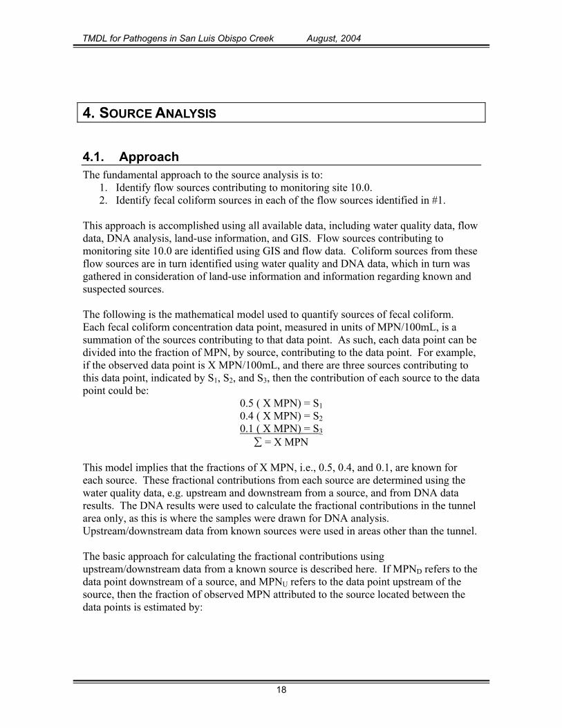
4.1. Approach The fundamental approach to the source analysis is to:
1. Identify flow sources contributing to monitoring site 10.0. 2. Identify fecal coliform sources in each of the flow sources identified in #1.
This approach is accomplished using all available data, including water quality data, flow data, DNA analysis, land-use information, and GIS. Flow sources contributing to monitoring site 10.0 are identified using GIS and flow data. Coliform sources from these flow sources are in turn identified using water quality and DNA data, which in turn was gathered in consideration of land-use information and information regarding known and suspected sources. The following is the mathematical model used to quantify sources of fecal coliform. Each fecal coliform concentration data point, measured in units of MPN/100mL, is a summation of the sources contributing to that data point. As such, each data point can be divided into the fraction of MPN, by source, contributing to the data point. For example, if the observed data point is X MPN/100mL, and there are three sources contributing to this data point, indicated by S1, S2, and S3, then the contribution of each source to the data point could be:
0.5 ( X MPN) = S1 0.4 ( X MPN) = S2 0.1 ( X MPN) = S3
∑ = X MPN This model implies that the fractions of X MPN, i.e., 0.5, 0.4, and 0.1, are known for each source. These fractional contributions from each source are determined using the water quality data, e.g. upstream and downstream from a source, and from DNA data results. The DNA results were used to calculate the fractional contributions in the tunnel area only, as this is where the samples were drawn for DNA analysis. Upstream/downstream data from known sources were used in areas other than the tunnel. The basic approach for calculating the fractional contributions using upstream/downstream data from a known source is described here. If MPND refers to the data point downstream of a source, and MPNU refers to the data point upstream of the source, then the fraction of observed MPN attributed to the source located between the data points is estimated by:
18

TMDL for Pathogens in San Luis Obispo Creek August, 2004
MPND - MPNU = ∆MPN
Source fraction (e.g. S1) = ∆MPN MPND
This source fraction is then applied to the remaining MPN, i.e., after the background fraction (81 MPN) is subtracted. For example, if the observed data point is 500 MPN, and fraction attributed to source1 is 0.25, then:
500 MPN – 81 MPN (background contribution) = 419 MPN
(419 MPN) (0.25) = 105 MPN
Therefore, Source1 is attributed 105 MPN of the total 500 MPN observed. Once the contribution in MPN is calculated for each source, concentration data and its corresponding flow data are used to calculate mass loading for that source. Adjusted flow values are used for some sources, e.g. livestock, because the upstream/downstream data used to derive livestock contributions were gathered at sites further upstream, where flow volume is less than the downstream site where mass loading is calculated. Source loading is in turn used to calculate relative contributions for each source. In some cases, only three source categories, including the background source category, are present at a monitoring site. In this case, once one fraction of MPN is calculated, e.g. using the method described above, the third can be calculated because the background contribution is known (see Section 4.2). The method for deriving the fraction of observed MPN by source is discussed for each site in the “Individual Calculations” Section below. Results of the DNA analysis were used to determine fractional source contributions from the tunnel. The relative frequency of the human isolates identified was calculated as a percent of the total isolates. This frequency was then used with concentration and flow data to estimate the mass loading from human sources in the tunnel. The approach described above does not consider factors as die-off and predation. However, staff consider this approach to be adequate for the following reasons:
1. The monitoring sites used in the TMDL calculations are relatively near each other (as will be seen), therefore die-off and predation will not have a large impact on the final TMDL.
2. The approach is by nature a conservative one because the actual number of organisms at downstream sites will be less than the model suggests. Therefore the approach lends itself to an implicit margin of safety through conservative assumptions.
19

TMDL for Pathogens in San Luis Obispo Creek August, 2004
Approach Inherently Conservative Staff considers this approach to be the best available method for determining contribution by source because the fraction of MPN attributed to a source is determined from highly localized data, and not literature values developed elsewhere. Furthermore, since staff collected data throughout the watershed and subwatersheds, as well as on a reach-by-reach basis along the main stem, source fractions of MPN are developed for each source occurring in a watershed. As a result, management practices, or the lack thereof, occurring in one subwatershed are not inferred to other subwatersheds.
Individual Calculations Hundreds of calculations were completed using spreadsheet formulas. The calculations and data used to develop the source analysis and TMDL are compiled in a spreadsheet model developed by staff titled “SLOPathTMDL” (RWQCB, 2004). The spreadsheet is referenced in the Reference section of this document. Reference to specific worksheets and cells are contained in this chapter. Many of the calculations used to develop the source analysis are contained in the worksheets titled “LOADING” and “SOURCE.”
4.2. Source Categories Staff identified 5 source categories. The source categories are based on:
DNA analysis results, • • •
land-use, consideration of implementing load reduction strategies.
The 5 source categories are:
1. background, 2. birds and bats in the tunnel (TBB), 3. urban, 4. human, 5. livestock.
The background fraction is estimated using Creek data gathered from areas draining relatively undisturbed lands. A total of nine data points drawn throughout the year indicate the mean background fecal coliform level is 81 MPN/100mL. Please see the accompanying spreadsheet “SLOPathTMDL,” worksheet “ANALAYSIS,” cell A1. The TBB fraction is a source category specific to San Luis Obispo Creek. This category refers to fecal contamination from animals that have populated an area in unusually high density. The congregation of these animals is brought on by creation of habitat along the stream. Specifically, this category refers to the tunnel area, where birds and bats are provided roosting habitat resulting in high population densities. DNA analysis (discussed below) of the tunnel area confirms this source category.
20

TMDL for Pathogens in San Luis Obispo Creek August, 2004
The urban source refers to sources originating in urban areas, including sources conveyed through storm drain conduits. This category includes coliform originating from pets, e.g. dogs and cats, as well as human waste not originating from point sources. The human source category refers to fecal coliform originating from potentially leaking private sewer lateral lines, illicit connections, or any other human source potentially entering the creek as a point source. The livestock source refers to range and confined animal sources. The relative small size of the watershed allows staff to identify areas where livestock sources are likely. In addition, monitoring data from subwatersheds support source analysis of this category.
4.3. Sources Contributing to Monitoring Site 10.0 The source analysis will focus on sources contributing to monitoring site 10.0, corresponding to the confluence with Stenner Creek and the main stem of San Luis Obispo Creek. Figure 4.1 illustrates the watershed areas being considered in the source analysis.
S an L
uis
Obi
spo
Cr.
Sten
ner Cr.
B rizzio la
ri C
r.
Garden Cr.
Site 10.0
City of San Luis Obispo
Watershed AreaDraining to Site 10.0
Streams
N0.6 0 0.6 1.2 Miles
Watershed Area Draining to Site 10.0
#
Figure 4.1 Watershed area draining to site 10.0
21

TMDL for Pathogens in San Luis Obispo Creek August, 2004
Note from the figure that there are two major flow sources to monitoring site 10.0, including: 1) Stenner Creek Watershed (a subwatershed of San Luis Obispo Creek Watershed), and 2) San Luis Obispo Creek main stem flow from the upper half of the watershed. Source analysis computations are made on these two flow sources with each flow source further delineated below. Fecal coliform sources from these two flow sources are then combined and expressed as the total load at monitoring site 10.0. The following discussion describes sources from the two main flow sources of Stenner Creek and the main stem of San Luis Obispo Creek.
Sources in Stenner Creek Watershed Stenner Creek Watershed is a subwatershed of San Luis Obispo Creek Watershed. The total area of Stenner Creek watershed is 7139 acres, with land-uses comprising the following proportions of the total area:
Range: 60.1% Agriculture: 10.4% Residential: 9.7% Commercial: 9.3%
Forest: 9.1% Utilities: 1.4%
Stenner Creek Watershed has been further delineated into four smaller subwatersheds, including:
Upper Stenner Watershed, • • • •
Lower Stenner Watershed, Brizzolara Creek Watershed, Garden Creek Watershed.
These delineations were made due to differences in land-use activity and potential coliform loading. The land-uses for the subwatersheds are articulated in Table 4.1 below. Table 4.1 Land-uses in Stenner Creek Watersheds
Subwatershed Land-use/Area (acres) name Agriculture Commercial Forest Range ResidentialUtilities Total
Upper Stenner 683 116 419 2990 0 34 4242 Lower Stenner 0 108 0 46 279 62 496 Brizziolari 0 286 175 1058 7 0 1526 Garden 61 153 52 199 409 0 875 TOTAL 744 663 646 4294 695 97 7139 % of Total 10.4 9.3 9.1 60.1 9.7 1.4 Note that most of the rangeland area in the watershed occurs in Upper Stenner and Brizzolara Creek subwatersheds. Lower Stenner and Garden Creek subwatersheds are
22
TMDL for Pathogens in San Luis Obispo Creek August, 2004
predominantly urbanized areas, draining stormwater flow as well as conveying flow from the upper watersheds.
Sources from Upper Stenner and Lower Stenner Creek Watershed Two monitoring sites in upper and lower Stenner Creek watershed are used to determine source loading. Monitoring site STEN3.0 is in the upper watershed, and is downstream of lands draining background, urban, and rangeland sources. The second monitoring site, STEN0.5, receives flow from Stenner Creek, and is near the confluence with San Luis Obispo Creek. The STEN0.5 monitoring site is located downstream of urbanized areas, draining both residential and commercial land-uses, and is within the City limits. Monitoring site STEN0.5 flows perennially, whereas monitoring site STEN3.0 flows seasonally. Figure 4.2 below illustrates the location of monitoring sites in Stenner Creek watershed.
BRIZ2.5
BRIZ1.0
BRIZ0.0
STEN3.0
STEN2.0A
STEN1.0
CHOR0.0 STEN0.5
Bri
zzio
lari C
r.
San L
uis
Obi
spo
Cr,
Stenner Cr.
wooden bridge
Garden Cr.
Monitoring Sites in Stenner Cr. Watershed
5000 0 5000 Feet
NCity of San Luis Obispo
#
#
#
#
#
##
#
Figure 4.2 Monitoring Sites in Stenner Creek Watershed
Note from Table 4.1 that range is the predominant landuse in Upper Stenner Creek watershed. Although the greatest proportion of the total area is designated as range land-use, only low-intensity grazing is present, with minimal or no access to riparian areas by grazing animals. The potential sources of fecal coliform in Upper Stenner Watershed are background, urban, and livestock. However, data from Upper Stenner Creek watershed indicate that
23

TMDL for Pathogens in San Luis Obispo Creek August, 2004
this watershed is achieving the numeric target. Consequently, no reductions of load in this watershed are necessary. Lower Stenner Creek lies within the city of San Luis Obispo. Fecal coliform loading in this area is attributed to urban sources.
Sources from Brizzolara Creek Watershed Brizzolara Creek watershed is a subwatershed of Stenner Creek Watershed. Three monitoring sites in Brizzolara Creek watershed are used to determine source-category loading. Monitoring site BRIZ2.5 is in the upper watershed draining forest and rangelands. Monitoring site BRIZ1.0 is also in the upper watershed, is located downstream of BRIZ2.5, and drains forest, range, and commercial lands. The third monitoring site is BRIZ0.0. BRIZ0.0 is located downstream of BRIZ2.5 and BRIZ1.0, and is immediately upstream of the confluence with Stenner Creek. BRIZ0.0 is located at the boundary of the City and Cal Poly and drains commercial and residential lands. Fecal coliform concentration increases between monitoring sites BRIZ2.5 and BRIZ1.0. Potential sources at site BRIZ1.0 include urban, livestock, and background. Sources contributing to load between sites BRIZ1.0 and BRIZ0.0 are background and urban. Brizzolara Creek is dry during summer and fall months. Consequently, no loading into San Luis Obispo Creek of fecal coliform from Brizzolara Creek is present during these seasons.
Sources from Garden Creek Watershed One water quality-monitoring site is used in Garden Creek to determine source loading. Monitoring site CHOR0.0 is located at the mouth of Garden Creek near its confluence with Stenner Creek (see Figure 4.2 for location). Garden Creek watershed is largely an urban watershed, draining stormwater through open channel flow. The narrow, and often channelized, creek meanders through residential and commercial areas. The headwaters of the creek are situated on a southeastern facing hillside visible from the residential areas. There are 199 acres of land designated for range. However, staff have observed that grazing occurs predominantly on the southwestern side of the hillside, draining to a different watershed. In addition, the headwaters of Garden Creek are most often dry, except following a rain event. Consequently, staff are confident that fecal coliform loading from livestock in this watershed is negligible. Two source categories have been identified in Garden Creek watershed, including: 1) background, and 2) urban. The background source contribution to fecal coliform MPN is 81 MPN/100mL, as explained in section 4.2. The urban fraction of MPN is simply calculated by determining the remaining MPN after background has been deducted.
24

TMDL for Pathogens in San Luis Obispo Creek August, 2004
Flow in Garden Creek is minimal, accounting for about 4% of the flow in Stenner Creek. As a result, fecal coliform load is low, relative to Stenner Creek.
San Luis Obispo Creek Main Stem Sources to Site 10.0 Two subwatersheds of San Luis Obispo Creek watershed contribute flow to monitoring site 10.0. The two subwatersheds are referred to as: 1) Upper and Reservoir, and 2) Upper City. The total area of the two watersheds is 8277 acres, with land-uses comprising the following portions of the total area:
Forest: 48.3% Range: 41.9%
Residential: 4.1% Commercial: 3.1%
Utilities: 2.6%
The Upper City subwatershed predominantly drains urban areas from the northeast portion of the City. The Upper and Reservoir subwatershed is comprised of forest, range, and utilities land-uses, with the former two land-uses comprising over 90% of the total area in this watershed. It is located outside the City limits at the eastern portion of the watershed, draining much of the headwaters of the main stem. Table 4.2 details the land-uses of these two watersheds. Table 4.2 Land-uses Contributing Flow to Site 10.0
Land-use/Area (acres) Subwatershed name Agriculture Commercial Forest Range Residential Utilities Total
Upper City 0 260 212 184 343 23 1022Upper and Reservoir 0 0 3786 3281 0 187 7255TOTAL 0 260 3998 3465 343 210 8277% of Total 0 3.1 48.3 41.9 4.1 2.6 Figure 4.3 illustrates the location of monitoring sites used to develop the source analysis from these watersheds.
25

TMDL for Pathogens in San Luis Obispo Creek August, 2004
Main Stem Monitoring Sites In Downtown Area
Site 12.5
Site 10.9
Site 10.3
Site 10.0
#
Tunnel Under City
Gard en Cr. Ste nner Cr.
San L
uis O
bispo
Cr.
#
Cuesta Park
City Boundary
SubwatershedBoundary
N
2000 0 2000 Feet
#
#
#
##
##
#
#
#
##
##
Figure 4.3 Main Stem Monitoring Sites in Downtown Area
Sources from Upper and Reservoir and Portions of Upper City Watersheds The main stem of the Creek flowing through the Upper City watershed can be delineated into two lengths: 1) downstream of the tunnel, and 2) upstream of the tunnel (refer to sections 3.1 and 4.2 for discussion of the tunnel). Recall that the Creek flows through approximately 1200 feet of a closed channel tunnel situated under the City. Fecal coliform levels downstream of the tunnel are significantly greater than those upstream of the tunnel. Consequently, the source analysis approach taken is to determine sources upstream of the tunnel as separate from the tunnel itself. Figure 4.4 illustrates fecal coliform concentration upstream and downstream of the tunnel. Data from monitoring site 10.9 is used to develop the source analysis in Upper and Reservoir subwatershed, as well as a portion of Upper City subwatershed upstream of the tunnel. Monitoring site 10.9 is immediately upstream of the tunnel, receiving flow from both of the aforementioned subwatersheds. Notice from Table 4.2 above that the predominant land-use in these subwatersheds is forest and range. Sources of fecal coliform from forested lands fall in the background source category.
26

TMDL for Pathogens in San Luis Obispo Creek August, 2004
Median Fecal Coliform Concentration Downstream and Upstream of Tunnel
0
200
400
600
800
1000
1200
1400
1600
1800
2000
DOWNSTREAM UPSTREAM
Feca
l Col
iform
(MPN
/100
mL)
TUNNEL
FLOW
Developed from 21 matching data points drawn over a two year period.
Figure 4.4 Median Fecal Coliform Values Upstream and Downstream from Tunnel
Rangelands potentially deliver fecal coliform from livestock. However, sources from livestock in this area are negligible. Staff are confident of this determination for the following reasons:
No livestock have been observed near the Creek in either of these watersheds in the two years of monitoring.
•
•
•
Access to the Creek for livestock is extremely limited as the Creek is dramatically incised in this area; stream banks are nearly vertical, dropping well over 10 feet to the waters edge. No DNA isolates from livestock were identified in 226 separate isolates identified. Samples used for the analysis were taken downstream of the range area.
Sources from utility, residential, and commercial land-uses are the remaining potential sources of fecal coliform, falling into the source category of urban. Therefore, Upper and Reservoir as well as the Upper City watersheds deliver: 1) background, and 2) urban sources. The background source contribution to fecal coliform MPN is 81 MPN/100mL, as explained in section 4.2; the remainder MPN from each data point is due to urban sources
Sources from the Tunnel The tunnel conveys flow for the main stem of the Creek for approximately 1200 feet under the downtown area of the City. The walls and ceiling are concrete while the bottom is natural for most of its length; there is a 200-300 foot section of concrete bottom. Private sewer laterals and water pipes cross the tunnel near the ceiling, servicing the businesses situated above.
27

TMDL for Pathogens in San Luis Obispo Creek August, 2004
The tunnel has created habitat for both pigeons and bats. Pigeons roost above the stream along the ledges at the tops of walls. Bats have found suitable habitat in crevasses of floor joists supporting the businesses overhead. Pigeon and bat guano builds up along the walls in some areas. Walls are subsequently washed following rain events. Monitoring site 10.9 is upstream of the tunnel along the main stem of the Creek. Data from this monitoring site are used to calculate loading from Upper and Reservoir as well as Upper City watersheds. Monitoring site 10.3 is located immediately downstream from the tunnel along the main stem of the Creek. The difference in coliform concentration between site 10.3 and 10.9 is used to determine sources delivered from the tunnel. In addition to concentration data, DNA analysis was performed on 27 samples taken from within the tunnel. A total of 226 isolates were extracted to determine sources of E. coli in the tunnel. Of the 226 isolates extracted, 27 could not be identified, i.e., the source is unknown. The 199 isolates identified are summarized in the graph below. The bars denote the number of isolates identified for a particular source. The lines/points denote the frequency (in percent) of an identified source relative to the total number of identified sources. For example, for the human category, 41% = 82/199 * 100%.
Total Number of Identified Isolates and Corresponding Frequency
34 3022
9 7 7 6 2
82
41
17 15 105 134 4
0
20
40
60
80
100
human
avian CSO
canin
erod
ent
dog
racoo
nfel
ine
opos
sum
Source
No.
of I
sola
tes
0
20
40
60
80
100Fr
eque
ncy
of
Iden
tifie
d So
urce
(%
)
No. of isolatesFrequency of known (%)
Figure 4.5 DNA identified sources of E. coli in tunnel.
Note from Figure 4.5 that 82 E. coli isolates were identified as originating from a human source. This number of identified isolates corresponds to 41.2% of the total identified isolates in the study.
28

TMDL for Pathogens in San Luis Obispo Creek August, 2004
The CSO source is combined sewer overflow. CSOs are used in some municipalities to convey sewer flow through storm conduits in the event of sewer overflow. The laboratory performing the DNA analysis drew samples from CSO flow in other watersheds and isolated a strain of E. coli only found in CSO sources. The strain of E. coli found in CSO sources from other watersheds is also present in the samples drawn from tunnel of San Luis Obispo Creek. Staff consider the CSO source an urban source in the Creek based on the following:
1. The sewer system of San Luis Obispo does not utilize CSOs. However, CSOs include flow from stormwater, which is considered an urban source.
2. The DNA isolates have not been attributed to a specific organism. Therefore, staff cannot justify attributing this isolate to an organism, e.g. human or livestock.
The frequency of the human isolates is 41.2%. Therefore, 41.2% of the difference in fecal coliform concentration between the upstream monitoring site 10.9, and the downstream monitoring site, 10.3, is attributed to the human source at site 10.3. The remaining 58.8% of the difference between downstream and upstream concentrations is divided between background, TBB, and urban sources. Urban sources are the combined frequencies of canine, dog, CSO and feline, contributing 32.7% of the total MPN. The TBB source (birds and bats in the tunnel), calculated by summing the avian and rodent fractions, is 21.6% of the total number of isolates identified. The background source is accounted for in the tunnel by using a fecal concentration of 81 MPN/100mL. Therefore, the increase in Creek fecal coliform concentration after flowing through the tunnel is attributed to the following sources and their corresponding contributions to the increase:
human: 41.2% TBB: 21.6% urban: 32.7%
The mathematical model for the sources in the tunnel, for each matched data point, therefore becomes:
MPN10.3 – MPN10.9 = ∆MPN human fraction = 0.412(∆MPN) TBB fraction = 0.216(∆MPN) urban fraction = 0.327(∆MPN)
Where MPN10.3 is a downstream data point, and MPN10.9 is an upstream data point. If there is not an increase in MPN at the downstream end on a sampling day, then sources from the tunnel are considered zero for that sampling period. This occurred in 3 of 20 total sampling events. Monitoring site 10.89 is a source discharging flow into and within the tunnel. Flow from this monitoring site discharges to the Creek through a concrete box drain, draining flow
29

TMDL for Pathogens in San Luis Obispo Creek August, 2004
from an urbanized area of the City. Fecal coliform concentration at site 10.89 is high, relative to the numeric target. The following is a set of summary statistics for the site:
Number of data points (for 2 years): 20 Minimum fecal MPN/100mL: 20
Maximum fecal MPN/100mL: 16,000 Median of data: 1,250
Log mean of data: 1,044 Discharge ratio to Creek: 0.04
Notice from the summary statistics that although the fecal coliform concentration exceeds the numeric target, that the total discharge volume from site 10.89 was 0.04 of the flow in the Creek at the discharge area. Consequently, the impact of discharge from 10.89 to Creek fecal coliform concentration is not as great as the concentration of the source may suggest. However, site 10.89 is discussed because it is a point source, and therefore subject to implementation tools different than non-point sources.
4.4. Summary of Source Analysis Recall from Section 4.3 that the approach taken in the source analysis is to determine the sources contributing to monitoring site 10.0, which is immediately downstream of the confluence of Stenner Creek and the main stem of San Luis Obispo Creek. Flow and coliform concentration data are available for both Stenner Creek and the main stem of San Luis Obispo Creek at monitoring points upstream of their confluence. Therefore, relative loading from each source is calculated. This is accomplished by first determining the fractional source contribution for each data point, using the methods described above. The fractional source contributions were then multiplied by the corresponding flow data to derive loading by source for both Stenner and San Luis Obispo Creek. The summation of the loading for each source from each watershed results in the total loading occurring at monitoring site 10.0. Relative contributions of the total load were then determined by source and watershed. Results from DNA analysis drawn from samples in main stem were not applied to Stenner Creek. Table 4.3 shows the resulting contribution, by source, to the observed coliform concentration occurring in Stenner Creek. Concentration data was obtained from samples at site STEN0.5, which is near the confluence with San Luis Obispo Creek.
30

TMDL for Pathogens in San Luis Obispo Creek August, 2004
Table 4.3 Relative Source Contributions to Coliform Concentration in Stenner Cr.
Stenner Cr. Data Relative Contributions To Concentration by Source In Stenner Creek
Contribution timeinterval Date of
Data
Fecal Coliform
(MPN/100mL) Flow
(ft3/sec) From To Background
(%) Livestock
(%) Urban
(%) Human
(%) TBB (%)
03/23/01 110.00 18.10 03/23/01 03/28/01 39 23 38 0 0 03/28/01 240.00 18.10 03/28/01 04/06/01 25 21 54 0 0 04/06/01 300.00 8.67 04/06/01 05/18/01 15 37 48 0 0 05/18/01 300.00 2.50 05/18/01 07/23/01 11 52 37 0 0 07/23/01 500.00 1.88 07/23/01 09/12/01 12 0 88 0 0 09/12/01 900.00 1.40 09/12/01 10/24/01 11 9 80 0 0 10/24/01 500.00 1.01 10/24/01 11/15/01 2 78 20 0 0 11/15/01 3000.00 0.80 11/15/01 11/30/01 1 31 68 0 0 11/30/01 9000.00 3.13 11/30/01 01/14/02 1 38 61 0 0 01/14/02 240.00 2.44 01/14/02 03/21/02 27 22 51 0 0 03/21/02 170.00 1.29 03/21/02 04/23/02 23 28 49 0 0 04/23/02 240.00 2.04 04/23/02 07/31/02 24 28 48 0 0 07/31/02 300.00 0.87 07/31/02 09/16/02 28 0 72 0 0 09/16/02 130.00 0.29 09/16/02 12/03/02 23 21 56 0 0 12/03/02 500.00 0.45 12/03/02 01/16/03 21 34 45 0 0 01/16/03 240.00 2.24 01/16/03 03/05/03 27 26 47 0 0 03/05/03 170.00 2.42 See accompanying spreadsheet “SLOPathTMDL,” worksheet “SOURCE,” cell J109. Note from Table 4.3 that the contribution to fecal coliform concentration by livestock is zero during the late summer months. This is so because the livestock sources occur in the upper watersheds where stream flow does not exist in late summer. When the livestock is minimal or non-existent, then the urban source is responsible for the greater proportion of observed concentration. Table 4.4 shows the contributions, by source, to the observed coliform concentration occurring in San Luis Obispo Creek immediately upstream of the confluence with Stenner Creek. Concentration data was obtained from samples collected at monitoring site 10.3. Corresponding flow data is also given. Recall that (as discussed above) results of the DNA analysis were considered in the source analysis for this site. An example calculation is provided in Appendix B.
31

TMDL for Pathogens in San Luis Obispo Creek August, 2004
Table 4.4 Relative Contributions to Coliform Concentration in Main Stem upstream of confluence with Stenner Cr.
San Luis Obispo Cr. Data Relative Contributions To Concentration by Source
in San Luis Obispo Creek Contribution time
interval Date of Data
Fecal Coliform
(MPN/100mL) Flow
(ft3/sec) From To Background
(%) Livestock
(%) Urban
(%) Human
(%) TBB(%)
03/22/01 240.00 18.06 03/22/01 03/28/01 23 0 43 22 12 03/28/01 500.00 14.70 03/28/01 04/06/01 9 0 36 36 19 04/06/01 1600.00 9.66 04/06/01 04/13/01 8 0 36 37 19 04/13/01 500.00 8.51 04/13/01 04/18/01 11 0 78 7 4 04/18/01 500.00 12.73 04/18/01 05/18/01 7 0 68 16 9 05/18/01 2400.00 3.90 05/18/01 07/23/01 3 0 38 39 20 07/23/01 3000.00 1.35 07/23/01 09/13/01 1 0 35 42 22 09/13/01 24000.00 0.73 09/13/01 10/24/01 1 0 35 42 22 10/24/01 9000.00 0.66 10/24/01 11/15/01 2 0 41 37 20 11/15/01 1600.00 1.00 11/15/01 11/30/01 13 0 52 23 12 11/30/01 500.00 6.40 11/30/01 01/14/02 8 0 40 34 18 01/14/02 2300.00 3.23 01/14/02 03/21/02 2 0 37 40 21 03/21/02 9000.00 2.54 03/21/02 04/23/02 1 0 37 41 21 04/23/02 9000.00 2.66 04/23/02 07/31/02 1 0 36 41 22 07/31/02 24000.00 0.85 07/31/02 09/18/02 1 0 35 42 22 09/18/02 13000.00 0.49 09/18/02 09/19/02 1 0 39 39 21 09/19/02 5000.00 0.49 09/19/02 11/27/02 3 0 65 21 11 11/27/02 1600.00 0.71 11/27/02 01/16/03 19 0 73 5 3 01/16/03 235.00 4.28 01/16/03 03/05/03 24 0 69 5 2 03/05/03 400.00 2.83 See accompanying spreadsheet “SLOPathTMDL,” worksheet “SOURCE,” cell J238. Note from Table 4.4 that there is not a livestock source to the main stem above monitoring site 10.3. Also note that the human and TBB sources, originating from the tunnel source, are lower in April 2001, November 2002, and March 2003, relative to other time periods. This is so because during these months there was not an increase in fecal coliform concentration between the downstream and upstream end of the tunnel. Consequently, only sources originating upstream of the tunnel are present for these data periods. Conversely, the human contribution to observed coliform concentration is highest during summer months. It is during these months that flow is minimal through the tunnel, so concentrations are greater, relative to wetter seasons. This is indicative of a consistent source of fecal coliform. In addition, Creek flow is zero in the upper portion of the main stem watershed, resulting in a greater contribution from urban sources to the observed concentration.
32

TMDL for Pathogens in San Luis Obispo Creek August, 2004
The resulting combined contribution by source to fecal coliform levels is given in Table 4.5. The contributions illustrate the combined sources from Stenner and San Luis Obispo Creek occurring immediately below their confluence. The values given are calculated based on observed loading in each watershed, which is a function of observed coliform concentration and flow. Therefore, the resulting contributions represent weighted averages, and not arithmetic averages, of the data observed in each watershed. An example calculation is provided in Appendix B. Table 4.5 Relative Contributions to Coliform Concentration in San Luis Obispo Creek.
Relative Contribution to Concentration by Source at Confluence of Stenner and San Luis Obispo Creek Contribution time
Interval From To
Background (%)
Livestock (%)
Urban (%)
Human (%)
TBB (%)
03/22/01 03/28/01 29 9 41 14 7 03/28/01 04/06/01 14 6 42 25 13 04/06/01 04/13/01 8 * 36 37 19 04/13/01 04/18/01 11 * 78 7 4 04/18/01 05/18/01 9 11 62 12 6 05/18/01 07/23/01 5 10 38 31 16 07/23/01 09/13/01 2 0 40 38 20 09/13/01 10/24/01 1 1 38 39 21 10/24/01 11/15/01 2 44 29 16 9 11/15/01 11/30/01 3 26 66 3 2 11/30/01 01/14/02 3 29 56 8 4 01/14/02 03/21/02 3 1 37 39 20 03/21/02 04/23/02 2 1 37 39 21 04/23/02 07/31/02 1 1 36 41 21 07/31/02 09/18/02 1 0 35 42 22 09/18/02 09/19/02 1 * 39 39 21 09/19/02 11/27/02 3 * 65 21 11 11/27/02 01/16/03 20 12 63 3 2 01/16/03 03/05/03 25 10 60 3 2 *The contribution from this source is accounted for in an adjacent data period. Necessary when days of data collection in Stenner and San Luis Obispo Creeks were not exactly the same. See accompanying spreadsheet “SLOPathTMDL,” worksheet “SOURCE,” cell B293. Note from the table above that the background source contribution to coliform concentration fluctuates from 1-29%. Recall that that background source contribution to concentration is 81 MPN/100mL. Also recall that the water quality objective for the protection of water contact recreation (REC-1) is 200 MPN/100mL. Therefore, any background value in the table above that is less than 40.5% (81 ÷ 200 *100%) indicates that conditions in the Creek are not meeting the REC-1 objective. Specifically, there were no time intervals from March 2001 to March 2003 where the fecal coliform levels
33
TMDL for Pathogens in San Luis Obispo Creek August, 2004
met the REC-1 objective, resulting from the combined concentrations from Stenner and San Luis Obispo Creek. The combined contribution of the urban and human sources to fecal coliform concentration account for a large portion of the observed levels. Note from the table above that for 18 of the 19 data periods, the combined contribution of urban and human sources is greater than 50%. The greatest livestock contributions occurred following some of the first rain events in 2001, i.e., November through January. Since the 2001 rain season, Cal Poly has made efforts to reduce loading from livestock by reducing cattle access in riparian areas. Finally, notice that the tables above articulate source contributions occurring in an interval of time. The intervals are defined by the number of days occurring between sampling events. The intervals are not equal, but based on several factors occurring during the monitoring period. As such, a contribution of a source in a shorter time interval will not have as much impact to water quality as one occurring in a larger interval. Figure 4.6 illustrates the weighed average contribution for each source category; the weighted average considers the interval of time that the contribution occurred, and is expressed as a percentage of the total contribution occurring over the two-year monitoring period. Notice from the figure that the urban and human source contributions are the greatest. This result is reasonable because the source analysis focused on an urban setting in an area where leakage from private sewer lines is documented. See spreadsheet SLOPathTMDL, “SOURCE” worksheet, cell J295. See example calculation in Appendix B. Weighted Average Contributions to Fecal Coliform
Concentration in San Luis Obispo Cr.
Human27%
Urban46%
Background6%
Livestock7%
TBB14%
Figure 4.6 Relative Contributions by Sources to Fecal Coliform Concentration in San Luis Obispo Cr.
34

TMDL for Pathogens in San Luis Obispo Creek August, 2004
4.5. Point and Non-Point Sources The distinction between point and non-point sources of fecal coliform contamination is necessary because reduction of each may be accomplished differently. Point sources of pollution are federally regulated through the National Pollutant Discharge Elimination System (NPDES). As such, a discharge is allowed through a permit and is done so under a set of parameters outlined in the permit. Non-point sources may be regulated through a Waste Discharge Requirement (WDR) from the Regional Board stating specific requirements of an identified responsible party(s).
Point Sources Point sources of fecal coliform to site 10.0 include: 1) sources from storm water, and 2) sources from sewage, including leaking private lines. Storm water collects flow from dispersed sources of fecal coliform, but because the flow is conveyed through a channelized and identifiable structure, it is considered a point source. The flow from monitoring site 10.89, as discussed above, is considered a point source, and is regulated through a storm water permit. Leakage from sewage collection systems is also considered a point source. The City’s waste water treatment plant (WWTP) discharges under an NPDES permit. The discharge is a point source of fecal coliform. However, recall from the Data Analysis Summary Section that the discharge carries fecal coliform concentrations less than 3 MPN/100mL. As such, the discharge significantly dilutes the more elevated coliform concentration flow from upstream. Furthermore, the source analysis is focused on sources upstream of the WWTP discharge. Therefore, the point discharge from the WWTP is not part of the source analysis or implementation/monitoring plan.
Non-Point Sources Non-point sources of fecal coliform are those contributing load over a dispersed area. Examples of non-point sources include livestock, pets, and wild animals. Livestock are potentially contributing to fecal coliform loading in upper Stenner watershed, as well as Brizzolara Creek watershed. Both of these sources of loading from livestock are discussed in the source analysis section. Pets and other domesticated animals are also contributing to coliform loading. Recall from the DNA analysis that dogs and cats are identified sources at the tunnel area. Staff have also witnessed contamination from dogs at the waters edge in the downtown area of the city. Contamination from human sources can originate from non-point sources. Both people recreating near the Creek, or those living near it at homeless encampments can be a source of fecal coliform. Staff have observed contamination from this source along the waters edge.
35

TMDL for Pathogens in San Luis Obispo Creek August, 2004
5. CRITICAL CONDITIONS AND SEASONAL VARIATION The critical conditions of impairment occur when fecal coliform levels rise above 200 MPN/100mL. This level is used because it is the water quality objective gauging the protection of the water contact recreation beneficial use (see Project Definition section). Exceedence of this water quality objective is considered critical (for this analysis) when:
1. A prolonged exceedence of the objective occurs. 2. When the exceedence is consistent throughout one or more seasons.
Exceedence of the water quality objective is normally measured by calculating the log mean of sample data from a monitoring site. A log mean is used because fecal coliform levels can be highly variable, subject to plums of fecal contamination resulting in high levels for a short duration. The log mean reduces the sensitivity to outliers, or unusually high concentrations. Figure 5.1 below (re-illustrated from previous section) illustrates the seasonality of fecal coliform concentration through several graphs. Fecal coliform concentrations are illustrated as log means. Note that fecal coliform levels are predominantly less than the 200 MPN/100mL threashold downstream of site 10.0 for all seasons. The only exception is in March/April of 2001, when sampling occurred during relatively high creek flow. As a result, fecal coliform loading occurring in the downtown area was carried through the system to monitoring sites downstream. Dilution occurred at site 6.67, where the City’s WWTP discharges nearly coliform free tertiary treated effluent. This dilution is further evident during dry seasons when coliform concentration is substantially diluted downstream of the discharge. Recall that it is this phenomenon that served as a basis for using site 10.0 as the focal point of the source analysis. Also note that critical conditions occur between sites 10.0 and 10.9, corresponding to the downtown area of the City. Particularly see that sites 10.0 and 10.3 exceed the threshold value of 200 MPN/100mL for all seasons, although the greatest exceedence occurs in July through September.
36

TMDL for Pathogens in San Luis Obispo Creek August, 2004
San Luis Obispo Cr.: Log Mean of Fecal Coliform from
5 Samples in 30d period (March/April01)
174 192 168217 206 195
675
545
225162
0100200300400500600700800900
1000
1.9 2.5 4.3 5.4 6.6 6.67 10 10.3 10.9 12.5
Site (distance upstream from mouth in miles)
Feca
l Col
iform
(MPN
/100
mL)
Log Mean of Fecal Coliform for July/Sept/Oct01
165 255 114 142 230
4626
8653
223 3380
100020003000400050006000700080009000
10000
1.9 2.5 4.3 5.4 6.67 10.0 10.3 10.9 12.5
Site (Distance upstream in miles)
Feca
l Col
iform
(MPN
/100
mL)
Log Mean for Fecal Coliform in Jan/Mar/Apr02
93 75 30 23 32 20 51
2664
4862
36864
0
1000
2000
3000
4000
5000
6000
1.9 2.5 4.3 5.4 6.0 6.6 6.67 10.0 10.3 10.9 12.5
Site (Distance upstream in miles)
Feca
l Col
iform
(MPN
/100
mL)
Log Mean of Fecal Coliform for Jul/Sept02
177 300 51 17 300 849
11598
4050
2000
4000
6000
8000
10000
12000
14000
1.9 4.3 6.0 6.6 6.67 10.0 10.3 10.9
Site (Distance upstream in miles)Fe
cal C
olifo
rm (M
PN/1
00m
L)
Log Mean of Fecal Coliform in Jan/Mar03
17940 30
200
2072
296 292117
0
500
1000
1500
2000
2500
1.9 2.5 5.4 6.0 10.0 10.3 10.9 12.5
Site (Distance upstream in miles)
Feca
l Col
iform
(MPN
/100
ml)
San Luis Obispo Cr.: Log Mean of Fecal Coliform for March/April 2003; 5 Samples in 30 days
1.7
183124
948
0100200300400500600700800900
1000
0.0 6.0 10.3 12.5
Site (Approximate distance upstream in miles)
Fec
al C
olifo
rm
(MPN
/100
mL)
Downtown area
WWTP Discharge
Upstream
Figure 5.1 Seasonal Coliform Concentrations
37

TMDL for Pathogens in San Luis Obispo Creek August, 2004
6. NUMERIC TARGET The objective of setting numeric targets is to protect existing beneficial uses as well as facilitate a TMDL calculation. Protection of some beneficial uses of the Creek is dependent on the levels of pathogenic organisms and the relationship of fecal coliform to pathogens. Pathogenic organisms are organisms that cause disease, particularly bacteria, virus, and protozoa. It is not feasible for agencies to analyze waters for all potential pathogenic organisms. Rather, an indicator organism is often used to suggest whether other pathogenic organisms are present. Agencies often differ in the use of indicator organisms, resulting in varying threashold values indicating whether or not a beneficial use is being protected. The Basin Plan of the Central Coast Regional Water Quality Control Board outlines two water quality objectives pertinent to this TMDL. The first is in place for the protection of non-contact water recreation (REC-2), and states:
“Fecal coliform concentration, based on a minimum of not less than five samples for any 30-day period, shall not exceed a log mean of 2000 MPN per 100mL, nor shall more than 10% of total samples collected
during any 30 day period exceed 4000 MPN per 100mL.” (Water Quality Control Plan, 1994)
A more stringent water quality objective protects water contact recreation (REC-1), and states:
“Fecal coliform concentration, based on a minimum of not less than five samples for any 30-day period, shall not exceed a log mean of 200 MPN per 100mL, nor shall more than ten percent of total samples
during any 30-day period exceed 400 MPN per 100mL.” (Water Quality Control Plan, 1994) Note that both objectives use fecal coliform as an indicator for pathogenic organisms. Since both REC-1 and REC-2 beneficial uses are present in the Creek, the more stringent of the two would be a more protective numeric target. The San Luis Obispo County Environmental Health Services (EHS) has also established bacteria levels for the protection of water contact recreation. The agency routinely samples waters at local beaches and may post a beach as unsafe if threshold levels are exceeded. The standards are as follows:
Total coliform concentration shall not exceed 10,000/100 mL of sample, or Fecal coliform shall not exceed 400/100mL of sample, or Enterococcus shall not exceed 61/100mL of sample, and
E. coli shall not exceed 235/100mL of sample.
Note that the EHS threashold using fecal coliform is less stringent than the Basin Plan objective. Also note that in addition to the use of fecal coliform as an indicator, that total enterococcus, and E. coli are also used.
38

TMDL for Pathogens in San Luis Obispo Creek August, 2004
The Environmental Protection Agency has suggested that E. coli and enterococci are a better indicator of the presence of pathogenic organisms, relative to fecal and total coliform. Regional Board staff are currently pursuing the use of E. coli and enterococci as indicator organisms and inclusion in the Basin Plan. However, it is not expected that new water quality objectives using these organisms will be in effect in a timeframe suitable to implement this TMDL. In addition, approval of proposed water quality objectives is not eminent. Therefore, the numeric target for the development of this TMDL is based on existing water quality objectives for the protection of water contact recreation. Staff make this determination based on the discussion above. The numeric target is:
Fecal coliform concentration, based on a minimum of not less than five samples for any 30-day period, shall not exceed a log mean of 200 MPN per 100mL, nor shall more than ten percent of total samples
during any 30-day period exceed 400 MPN per 100mL The value of 200 MPN/100mL is used to develop the TMDL and allocations in the sections that follow.
39

TMDL for Pathogens in San Luis Obispo Creek August, 2004
7. LINKAGE ANALYSIS The linkage analysis describes the cause and effect relationship between the sources of a pollutant and the numeric target. In the case of this TMDL, the relationship sought is between fecal coliform loading into the Creek and the numeric target measuring fecal coliform concentration. The relationship between the source and numeric target for this TMDL is clear; the numeric target is a direct measurement of the presence of coliform. Consider the following:
1. Source of pollutant is fecal coliform. 2. Fecal coliform are organisms, so can be individually counted. 3. Fecal coliform individuals (the source) present in the Creek can be quantified by
the number of individuals occurring in a volume of water, i.e., Number of individuals per volume of water, or no./volume. •
4. The units of the numeric target are numbers of individuals per volume of water, referred to as most probable number (MPN) per volume of water.
Note that the numeric target described in bullet-4 above is a quantification of the source, described in bullets 1-3 above. Therefore, the relationship between the source and the numeric target is clear. As such, as fecal coliform loading increases, the units of no./volume, expressed as most probable number (MPN), will also increase. Therefore, letting α imply proportionality:
Fecal coliform load α MPN
If loading is indeed proportional to concentration, measured in MPN, then it would follow that in areas where fecal coliform loading is present, a corresponding increase in MPN would occur downstream of the loading. This is the case at the downstream end of the tunnel (see Source Analysis section discussion). Fecal coliform loading from birds and bats is apparent within the tunnel, and verified through DNA source analysis. A corresponding significant increase in numbers of coliform, measured in MPN, occurs downstream of this loading, thereby supporting the linkage analysis.
40

TMDL for Pathogens in San Luis Obispo Creek August, 2004
8. TMDL CALCULATION AND ALLOCATIONS The TMDL and allocations are expressed in units of receiving water fecal coliform concentration. This unit is consistent with the numeric targets used to gauge achievement of the TMDL. Fecal coliform concentration is a function of both numbers of coliform and volume of water. As such, the maximum coliform loading allowed while still achieving the numeric target is not static; greater loading can occur during higher flow volume. Flow volume in the Creek changes seasonally. Therefore, meeting the numeric target, and achieving the TMDL, may require a different set of management strategies through seasonal changes; or at least, offers the possibility of varying management strategies on a seasonal basis.
8.1. Allocations The TMDL fecal coliform concentration has been allocated equally to all locations and sources. Figure 8.1 illustrates the sites referenced in Table 8.1. Table 8.1 shows the allocations geographically. Note that each allocation in Table 8.1 includes the allocation to background. Allocations are stated as waste load allocations (WLA) or load allocations (LA) in Table 8.1, and are defined as such depending on the method of conveyance and regulation of the sources contributing to an allocation. The allocations are:
1. Site-referenced allocations are shown in Table 8.1 below. Site-referenced concentrations refer to receiving water fecal coliform concentrations measured as a log mean of 5 samples drawn in a 30-day period occurring in the season noted.
2. For stream reaches not specifically noted in Table 8.1, the allocation for any
discharge discharging fecal coliform into San Luis Obispo Creek or any of its tributaries is as follows:
a. Fecal coliform concentration, based on a minimum of not less than five samples for any 30-day period, shall not exceed a log mean of 200 MPN per 100mL, nor shall more than 10% of the total samples during any 30-day period exceed 400 MPN per 100mL.
41

TMDL for Pathogens in San Luis Obispo Creek August, 2004
#
#
#
#
#
Br iz
zio
lari Cr.
Stenner Cr .
Garden Cr.
Site 10.0
STEN0.0
STEN1.5
BRIZ1.0
San Luis O bispo
Cr.
#
Site 12.5
Site 10.9
Figure 8.1 Allocation Reference Points
Locations of the sites illustrated on the map are described as follows:
Site 12.5: located along the main stem of the Creek at Cuesta Park. • •
•
•
•
•
Site 10.9: is located along the main stem of San Luis Obispo Creek at the upper (upstream) end of the tunnel, Site 10.0: is located along the main stem of San Luis Obispo Creek at the bridge crossing the Creek on Marsh Street. This location is downstream of the confluence of the main stem with Stenner Creek, STEN1.5: is located in Stenner Creek at its crossing with Highland Drive on Cal Poly campus, STEN0.0: is located at the mouth of Stenner Creek before its confluence with San Luis Obispo Creek; BRIZ1.0: is located in Brizzolara Creek at its crossing with Via Carte Drive on Cal Poly campus; this point is located downstream of the bull-test animal unit.
42
TMDL for Pathogens in San Luis Obispo Creek August, 2004
Table 8.1 Geographically-referenced Allocations
GEOGRAPHICALLY REFERENCED ALLOCATIONS AND RESPONSIBLE PARTIES
Allocations in San Luis Obispo Creek
From Site:
To Upstream Site:
Responsible Party 2, 3, 4
Allocation Type5
Contributing Sources
Receiving Water
Fecal Coliform Concentration (MPN/100mL)1
LA Background 12.5 All upstream
sites County
WLA Urban ≤ 200
LA Background 10.9 12.5 City
WLA Urban ≤ 200
LA Background 10.0 10.9 City
WLA Urban, Human, TBB
≤ 200
Allocations in Stenner and Brizzolara Creeks
From Site:
To Upstream Site:
Responsible Party 2, 3, 4
Allocation Type5
Contributing Sources
Receiving Water
Fecal Coliform Concentration (MPN/100mL)1
LA Background Livestock
STEN1.5 All upstream sites Cal Poly
WLA Urban ≤ 200
LA Background STEN0.0 STEN1.5 City
WLA Urban ≤ 200
LA Background Livestock BRIZ1.0 All upstream
sites Cal Poly WLA Urban
≤ 200
Allocations for reaches not specifically noted above: For stream reaches not specifically noted above, the allocation for any discharge loading fecal coliform into San Luis Obispo Creek or any of its tributaries is as follows: • Fecal coliform concentration, based on a minimum of not less than five samples for any 30-day period, shall not exceed a log mean of 200 MPN per 100mL, nor shall more than 10% of the total samples during any 30-day period exceed 400 MPN per 100mL.
1 As log mean of 5 samples taken in a 30-day period occurring within each season. 2 County implies County of San Luis Obispo 3 City implies City of San Luis Obispo 4 Cal Poly implies California Polytechnic State University, San Luis Obispo Campus 5 WLA implies Waste Load Allocation, LA implies Load Allocation The responsible parties noted in the table above are identified with respect to lands held by each responsible party and the sources of coliform identified as originating from held lands.
43

TMDL for Pathogens in San Luis Obispo Creek August, 2004
8.2. Wasteload Allocations Allocations to urban, human , and TBB sources in Table 8.1 are wasteload allocations. These allocations are wasteload allocations because regulation of these sources fall under NPDES permit laws and are regulated as such. Individual permit holders are discussed in the Implementation Plan section of this TMDL.
8.3. Load Allocations The allocation to livestock in Table 8.1 is the only load allocation.
8.4. Margin of Safety A margin of safety is required in the TMDL to account for inherent uncertainties. Uncertainties include:
1. Variability of flow. 2. Variability in fecal coliform concentration. 3. Accuracy of laboratory methods used to determine fecal coliform concentration.
Flow in the San Luis Obispo Creek watershed is highly variable. Rain events can drive flow volume to increase by orders of magnitude, but is also dependent on previous rain events. Base flow changes monthly as well as annually, implying annual changes in mass loading and assimilative capacity. The flow data used to calculate mass loading of fecal coliform represents the flow occurring at the time the water quality measurement (fecal coliform conentration) was determined. Two years of such data is used to estimate the assimilative capacity, and therefore TMDL. The TMDL utilizes fecal coliform conentration to determine mass loading of various sources. Concentration is estimated using multiple tube fermentation analysis to estimate the concentration in units of MPN, or most probable number of microbes per volume. Although this is an EPA approved method of analysis, there exists potential error. Staff have accounted for some of these uncertainties by developing concentration based allocations; if the allocation concentrations are achieved, the TMDL will be achieved, regardless of flow. In addition, staff have incorporated a margin of safety in the TMDL. The margin of safety is built into the TMDL through conservative assumptions. The conservative assumptions include: 1) low-flow data collection, 2) assumption of zero die-off, and 3) conservative numeric target.
Low-flow Data Collection The data used to develop the TMDL and allocations were collected over a two-year period begninning March 2001. Greater than 20 sampling days were used to collect over 400 fecal coliform concentration data. No sampling occurred during a rain event, although two sampling days occurred within 48 hours of a rain event. Consequently, the greatest proportion of data used to calculate the TMDL was collected during low-flow periods.
44

TMDL for Pathogens in San Luis Obispo Creek August, 2004
The range of flow observed at monitoring site 10.3 for the two years of record is 0.49-18.06 ft3/sec. The median value during the monitoring period was 2.74 ft3/sec. Therefore, most of the concentration data used to develop the TMDL was gathered at relatively low-flow conditions. It is during low-flow conditions that fecal coliform concentration is the greatest, relative to higher flows. As a result, the coliform concentrations used in the TMDL calculations are biased towards the greatest exceedence of the numeric target. Figure 8.2 below illustrates the fecal coliform concentration data as a function of the flow observed during the data collection. Two observations are noteworthy in Figure 8.2. First, note that the greatest portion of data collected was collected at flow levels less than 5 ft3/sec. This flow represents a fraction of the bankfull flow at monitoring site 10.3. Secondly, fecal coliform concentration increases exponentially during lower flow periods. Therefore, there is a conservative approach in the TMDL calculation because the data used to develop the TMDL is significantly biased in the direction of a worst-case-scenario.
Fecal Coliform Concentration as f(flow) at Site 10.3
0.005000.00
10000.00
15000.0020000.0025000.0030000.0035000.00
40000.0045000.0050000.00
0.00 5.00 10.00 15.00 20.00
Flow (cfs)
Feca
l Col
iform
(MPN
/100
mL)
Figure 8.2 Fecal Coliform Concentration Plotted Against Observed Flow at Site 10.3
Assumption of Zero Die-off and Predation The TMDL is developed on the basis of the numeric target of fecal coliform concentration. Fecal coliform are organisms inhabiting the intestines of warm-blooded animals. As such, die-off occurs in the stream environment. The rate of die-off is a function of species, temperature, solar-radiation, nutrient availability, and other environmental factors.
45

TMDL for Pathogens in San Luis Obispo Creek August, 2004
The TMDL was calculated with the assumption that there is zero die-off of fecal coliform. Consequently, observed increases in coliform concentration, including in the upper portions of the watershed, were assumed to translate into coliform loading at the monitoring points used to develop the TMDL and allocations. The zero die-off assumption also translates to a conservative approach to the allocation method. The allocations are expressed in units of fecal coliform concentration, and represent the allowable concentration for each source resulting in the numeric target, and therefore the TMDL. However, discharge of coliform from the sources at the allocated levels will in effect produce fecal bacteria concentrations in the Creek at levels lower than the numeric target; this is so because die-off is imminent, yet not accounted for. The assumption of zero predation is also a conservative approach. Similar to the zero-die off assumption, predation of fecal coliform by other organisms is inevitable. Microorganisms and macro-invertebrates in stream systems utilize bacteria, including fecal coliform, as a food source. Reduction of fecal coliform population, and therefore concentration, by predation is not accounted for in the TMDL calculations. In addition, predation is not accounted for in the allocation determination. Consequently, actual in-stream concentration will be lower than the numeric target if the various source-categories discharge at their respective allocations.
46

TMDL for Pathogens in San Luis Obispo Creek August, 2004
9. PUBLIC PARTICIPATION Public participation began when initial TMDL efforts were initiated in March 2001. The City of San Luis Obispo has been notified regarding results of staff monitoring efforts. Staff have also held several meetings with City officials to inform the City of the status of TMDL development, informing the City of:
proposed numeric targets, • • • •
locations of high coliform concentrations, problems associated with sources in the tunnel area, DNA results, including probable sewer-line leakage.
The City has consistently responded in a timely manner when advised that evidence suggested coliform sources were being conveyed through City infrastructure. In addition, staff were invited to give a presentation to the City council outlining TMDL efforts. The presentation and dialogue was broadcast via radio and cable television. Cal Poly has been notified of results of staff monitoring results. Like the City, Cal Poly has responded quickly and positively to reduce coliform loading through best management practices (as discussed in the Implementation Plan). In addition, Cal Poly has drafted and is implementing a campus Water Quality Management Plan (WQMP). The WQMP identifies management strategies that Cal Poly will utilize to reduce loading of pollutants, including fecal coliform. The citizens of the watershed have been informed and invited to comment on TMDL efforts. Regional Board staff have made presentations to local grass-roots organizations and have described results of monitoring efforts as well as suspected sources. Citizens and visitors to San Luis Obispo Creek have been informed of the risk associated with contact recreation in the Creek. Shortly after TMDL development began, the Department of Health posted the Creek at several locations, warning would-be waders of the risks associated with water contact recreation.
47

TMDL for Pathogens in San Luis Obispo Creek August, 2004
10. IMPLEMENTATION PLAN
10.1. Introduction The objective of the Implementation Plan is to articulate courses of action leading to achieving the TMDL. The sources of coliform in San Luis Obispo Creek (Creek) have been discussed in the previous sections. Knowledge of the origins and means of conveyance of bacterial sources to the Creek help staff determine regulatory mechanisms and actions that can be used to reduce coliform loading. The mechanisms and actions are discussed in this section.
10.2. Required Trackable Implementation Actions Implementation actions are required through existing or anticipated regulatory mechanisms. Regulatory mechanisms requiring implementation actions include:
1. National Pollutant Discharge Elimination System (NPDES) permits, a. Including the Storm Water Discharges from Small Municipal Separate
Storm Sewer Systems (Small MS4 Permit), 2. Waste Discharge Requirements (WDR). 3. Reporting and Monitoring pursuant to Section 13267 or 13383 of the California
Water Code The City of San Luis Obispo’s Water Reclamation Facility currently holds an NPDES permit allowing the discharge of tertiary treated wastewater to San Luis Obispo Creek. The City of San Luis Obispo, Cal Poly State University, and the County of San Luis Obispo are covered by the Small MS4 Permit to discharge stormwater to surface waters in the watershed. Cal Poly currently holds a WDR, permitting the irrigation of livestock wastewater to lands owned by Cal Poly. The following table outlines the schedule of the required implementation actions. The actions in the table below represent minimum actions and schedules required. The Regional Board may, at its discretion, alter the tasks defined below if sufficient water quality improvements are not realized. The Regional Board will make modifications to the tasks listed below pursuant to, but not limited to, the regulatory mechanisms articulated in the table. Also note that tasks requiring monitoring activities refer to monitoring efforts that are described in the Monitoring Plan, which is outlined in the next section of this document.
48

TMDL for Pathogens in San Luis Obispo Creek August, 2004
Table 10.1 Schedule and Trackable Implementation Actions of Responsible Dischargers
Implementing Party Source(s) Regulatory Mechanism(s) Action(s) of Implementing Party Schedule of Action(s)
1. Annual Report: Report specific measures that have been and/or will be taken to reduce fecal coliform loading from livestock and urban sources. Specifically address sources from:
a. Livestock along riparian areas. b. Runoff from grazing and confined
animals. Report monitoring results.
Submit Annual Report within one year after TMDL approval by the Office of Administrative Law and annually every year thereafter until numeric target achieved.
Livestock
Waste Discharge Requirements (WDR). Regional Board Executive Officer amendment of Monitoring and Reporting Requirements to incorporate reporting on specific implementation measures (creek monitoring and reporting on monitoring is already required).
2. Monitor pursuant to existing WDR monitoring requirements that are based on the TMDL monitoring plan.
Begin monitoring within one year after TMDL approval by the Office of Administrative Law. Report monitoring results annually with Annual Reports (see Action item #1).
Cal Poly State University
Urban Small MS4 Permit 4. Storm Water Management Plan (SWMP): Amend SWMP to include specific actions that have been and/or will be taken to reduce fecal coliform loading from urban sources.
5. Annual Report: Report specific measures that have and/or will be taken to reduce fecal coliform loading from urban sources.
Submit Annual Report within one year after TMDL approval by the Office of Administrative Law and annually every year thereafter until numeric target achieved.
49

TMDL for Pathogens in San Luis Obispo Creek August, 2004
Table 10.1 Continued: Schedule and Trackable Implementation Actions of Responsible Dischargers Implementing
Party Source(s) Regulatory Mechanism(s) Action(s) of Implementing Party Schedule of Action(s)
Urban Human TBB
Small MS4 Permit. Regional Board Executive Officer amendment of monitoring and reporting requirements to incorporate creek monitoring for fecal coliform and reporting of monitoring.
1. SWMP: Amend Storm Water Management Plan to include specific actions that have been and/or will be taken to reduce fecal coliform loading from urban, human, and TBB sources.
2. Annual Report: Report specific measures that have and/or will be taken to reduce fecal coliform loading from urban, human, and TBB sources. Specifically address sources from:
a. Domestic animals, b. Human sources, c. Animals attracted to the tunnel area.
3. Monitor: Monitor pursuant to Small MS4 Permit monitoring requirements, which are based on the TMDL monitoring Plan.
Report results of monitoring.
Submit Annual Report within one year after TMDL approval by the Office of Administrative Law and annually every year thereafter until numeric target achieved.
4. Annual Report: Report specific measures that have been and/or will be taken to reduce fecal coliform loading from human sources. Report results of monitoring.
Submit Annual Report within one year after TMDL approval by the Office of Administrative Law and annually every year thereafter until numeric target achieved.
City of San Luis Obispo
Human NPDES permit for WRF. Regional Board Executive Officer or Regional Board amendment of Monitoring and Reporting Requirements to incorporate creek monitoring for fecal coliform and reporting of monitoring.
5. Monitor: Monitor pursuant to NPDES permit monitoring requirements, which are based on the TMDL monitoring plan.
Begin monitoring within one year after TMDL approval by the Office of Administrative Law. Report monitoring results annually with Annual Reports (see Action item #4).
County of San Luis Obispo
Urban Small MS4 Permit 1. SWMP: Amend Storm Water Management Plan to include specific actions that have been and/or will be taken to reduce fecal coliform loading from urban sources.
2. Annual Report: Report specific measures that have and/or will be taken to reduce fecal coliform loading from urban sources.
Within one year after TMDL approval by the Office of Administrative Law and annually every year thereafter until numeric target achieved.
50
TMDL for Pathogens in San Luis Obispo Creek August, 2004
10.3. Responsibilities of Regional Board
Executive Officer or Regional Board Amends Monitoring and Reporting and Storm Water Management Requirements
The Executive Officer or the Regional Board will amend the monitoring and reporting requirements associated with NPDES permits or Waste Discharge Requirements, pursuant to 13383 or 13267 of the CA Water Code, respectively, to include specific requirements for reporting on implementation actions and monitoring required by this TMDL. The Executive Officer will also require modifications of the City’s Storm Water Management Plan pursuant to Section D of the Small MS4 Permit.
Regional Board Assessment Regional Board staff will assess progress towards meeting allocations and achieving the TMDL. In its assessment, the staff will utilize the annual reports submitted by implementing parties (listed in Table 10.1), results of monitoring efforts (described in Monitoring Plan section), and other information, to assess progress. Regional Board staff assessment will occur every three years, beginning at the end of the third year following approval of the TMDL. Assessments will continue until the TMDL is achieved. The Regional Board may require modifications to the Implementation and/or Monitoring Plan(s), including implementation actions, if, after each assessment, the Regional Board determines that fecal coliform reductions and/or the implementation actions have been inadequate or are unlikely to result in achieving the allocations.
10.4. Timeline and Milestones It is anticipated that the allocations, and therefore TMDL, will be achieved ten years from the date of approval of the TMDL. The estimation is based on the cost and difficulty inherent in identifying fecal coliform sources from all sources. The estimation is also based on the uncertainty of the time required for water quality improvement resulting from best management practices to be realized. Small MS4 permits outline a 5-year schedule for full implementation of best management practices (BMPs) and activities. In general, stormwater BMPs are designed to achieve compliance with water quality standards to the maximum extent practicable (MEP) through an iterative process. It is anticipated that the full in-stream positive effect of the BMPs will be realized gradually, and after full implementation of the BMPs. Staff therefore set a goal for TMDL attainment of ten years after TMDL adoption. In addition, stormwater permits may include additional provisions that the Regional Board determines are necessary to control pollutants. (CWA section 402(p)(3)(B)(iii).) The Regional Board can consider additional requirements if BMP implementation does not result in adequate water quality improvement.
51

TMDL for Pathogens in San Luis Obispo Creek August, 2004
10.5. Existing Efforts to Reduce Coliform Levels The City of San Luis Obispo has actively been identifying sources of fecal coliform contamination in the downtown area of the City, particularly within the tunnel. Efforts thus far include:
1. Mapping of sewer lines, storm drains, privately owned sewer laterals, and roof drains in the tunnel area to initiate identification of potential coliform sources.
2. Photographing sewer laterals and storm drain outlets for those identified in item-1 above.
3. Dye-testing private sewer laterals, and visually observing potential sewage leaks into the Creek from private laterals.
4. Corrective actions include seven notice of violations mailed to property owners regarding illegal sewage disposal. Six facilities have been required to make repairs to sewer laterals.
As discussed above, Cal Poly has reduced bacterial contamination by livestock by:
1. Installing fencing along Stenner and Brizzolara Creek to eliminate livestock access.
2. Installing fencing around storm-drain outlets adjacent to grazing areas. 3. Eliminating wastewater irrigation adjacent to surface waters. 4. Seeking to develop land areas currently used for concentrated livestock feeding.
The planned development is a student-housing project that is currently in the environmental review stage of planning.
10.6. Cost-estimate of Implementation A large portion of the identified loading in the watershed is from urban and human sources. As such, an estimate of cost can be made based on costs realized or anticipated by municipalities to reduce pollutant loading from these sources. Table 10.2 shows the estimated costs incurred by the City of Watsonville for implementing stormwater regulations. These estimates can be used to help gauge the costs of implementing the TMDL. The cost to the City of San Luis Obispo can be estimated by multiplying the population of the City by the total per capita cost. The cost of implementation for the city therefore is:
(Population) x (per-capita cost) = implementation cost 44,650 x $4.31 = $192,441 per year
The costs incurred by Cal Poly will be costs associated with reducing livestock and urban sources. The cost to reduce livestock sources have been accounted for, in part, due to existing plans to develop areas along Brizzolara Creek where livestock are currently located. Additional management activities may be required, but the costs of implementing the management efforts will be insignificant once the sources from Brizzolara are reduced.
52

TMDL for Pathogens in San Luis Obispo Creek August, 2004
The cost to reduce urban sources from Cal Poly can be estimated using Table 10.2 below. The cost to identify illicit connections will not be incurred by Cal Poly as human sources have not been identified as a source. Since this category is 11% of the total cost, the total cost per-capita to Cal Poly is estimated by:
0.89 x $4.31 = $3.84 The population at Cal Poly is approximately 17,000, therefore, the cost is estimated to be:
$3.84 x 17,000 = $65,280 per year
It is unlikely that actual costs to Cal Poly will be this high, as the University has a smaller area to cover, relative to the City of San Luis Obispo. The estimate is therefore a liberal one. Since the goal is to achieve the allocations in 10 years after adoption, the total cost of implementing the TMDL is estimated to be:
10 x ($192,441 + $65,280) = $2,577,210
Again, this figure is considered a liberal one because some of the control measures outlined in Table 10.2 may not be repeated every year. However, the overestimation will help account for any costs not explicitly accounted for. The following estimate is based on costs estimated by the City of Watsonville for implementing stormwater regulations (personal communication, Jennifer Bitting; RWQCB, September 2003): Table 10.2 Annual Cost Estimate of Implementation
Control Measure Activities Total Cost Public Education and Outreach
Brochures, advertising through media and businesses
$16,000
Public Participation Stormdrain stenciling, community clean-ups
$3,750
Stormwater Ordinance Draft to approval $2,100 Illicit discharge and detection
Program development, mapping, determining sources, correction
$3,750
Pollution prevention/Good-Housekeeping
Training, clean-up activities $1,900
Construction site runoff control
Education and training $2,400
Post-construction runoff control
Education and training $2,400
Permitting and reporting requirements
Development of good-housekeeping procedures
$700
Estimated Annual Program Costs
$33,750 per year
53

TMDL for Pathogens in San Luis Obispo Creek August, 2004
Per-capita program annual costs
$0.89/person
Street sweeping annual cost per-capita
$3.42
Total per-capita annual cost $4.31
11. MONITORING PLAN
11.1. Introduction The Monitoring Plan (Plan) outlines the monitoring sites, frequency of monitoring, and parties responsible for monitoring. The monitoring proposed below for TMDL compliance and evaluation is the minimum staff believes is necessary. However, if a change in these requirements is warranted after the TMDL is approved, the Executive Officer and/or the Regional Board will require such changes.
11.2. Monitoring Sites, Frequency, and Responsible Parties The sites illustrated in Figure 11.1 detail the locations of the required monitoring sites. The locations of the sites are described as follows:
Site 10.0: is located along the main stem of San Luis Obispo Creek at the bridge crossing the Creek on Marsh Street. This location is downstream of the confluence of the main stem with Stenner Creek.
•
•
•
•
•
•
Site 10.3: is located along the main stem of San Luis Obispo Creek at Mission Plaza, immediately downstream of the lower (downstream) end of the tunnel. Site 10.9: is located along the main stem of San Luis Obispo Creek at the upper (upstream) end of the tunnel. STEN0.0: is located at the mouth of Stenner Creek before its confluence with San Luis Obispo Creek. STEN1.5: is located in Stenner Creek at its crossing with Highland Drive on Cal Poly campus. BRIZ0.0: is located in Brizzolara Creek at its crossing with Via Carte Drive on Cal Poly campus; this point is located downstream of the bull-test animal unit.
Monitoring frequency will depend, in part, on whether the creeks illustrated in Figure 11.1 are flowing during a monitoring period. In particular, both Stenner and Brizzolara Creeks may be dry during late summer and fall. As such, stream samples may not be drawn during some seasons of dry years. Table 11.1 identifies the responsible party, monitoring site, sampling period, number of samples, and constituents to be monitored. Each sampling event assumes that flow is
54

TMDL for Pathogens in San Luis Obispo Creek August, 2004
present in the creek being sampled. If flow is not present, the responsible party must identify the date that monitoring was to occur, and state that flow was not present. Note from the table that the City and Cal Poly are responsible for monitoring, but the County is not. This is so because the highest fecal coliform concentrations have been observed on lands managed by the City and Cal Poly.
#
#
#
#
#
#
B rizz
io lar i C r .
S tenner Cr .
G ard en C r.
S ite 10 .0
ST E N0.0
Site 10 .3
ST EN1.5
BR IZ1 .0
S an Luis O b isp o C r
.S ite 10.9
Figure 11.1 Locations of Monitoring Sites
Table 11.1 Creek monitoring, responsible parties, sites, frequency, and constituent.
Responsible Party MonitoringSite
SamplingPeriod
Number ofSamples1
Constituent (in MPN/100mL)
10.0 Jan.-March 5 Fecal Coliform April-May 5 Fecal Coliform June-Sept. 5 Fecal Coliform Oct.-Dec. 5 Fecal Coliform
10.3 Jan.-March 5 Fecal Coliform April-May 5 Fecal Coliform June-Sept. 5 Fecal Coliform Oct.-Dec. 5 Fecal Coliform
10.9 Jan.-March 5 Fecal Coliform April-May 5 Fecal Coliform June-Sept. 5 Fecal Coliform Oct.-Dec. 5 Fecal Coliform
STEN0.0 Jan.-March 5 Fecal Coliform April-May 5 Fecal Coliform June-Sept. 5 Fecal Coliform
City of San Luis Obispo
Oct.-Dec. 5 Fecal Coliform STEN1.5 Jan.-March 5 Fecal Coliform Cal Poly State
University April-May 5 Fecal Coliform
55

TMDL for Pathogens in San Luis Obispo Creek August, 2004
June-Sept. 5 Fecal Coliform Oct.-Dec. 5 Fecal Coliform
BRIZ1.0 Jan.-March 5 Fecal Coliform April-May 5 Fecal Coliform June-Sept. 5 Fecal Coliform Oct.-Dec. 5 Fecal Coliform
1Five samples must be drawn in a 30-day period within each sampling period.
11.3. Reporting The parties responsible for implementation and monitoring will incorporate the results of monitoring efforts in the annual reports as described in Table 10.1 of the implementation plan. If reporting changes become necessary based on staff’s assessment of the TMDL implementation progress, the Executive Officer or the Regional Board will require such changes.
56

TMDL for Pathogens in San Luis Obispo Creek August, 2004
REFERENCES Regional Water Quality Control Board (RWQCB): Central Coast Region. 1994. Water Quality Control Plan: Central Coast Region. State of California, Sacramento California Regional Water Quality Control Board (RWQCB): Central Coast Region 2004. SLOPathTMDL.xls (an MS Excel spreadsheet model). San Luis Obispo, California. USEPA (United States Environmental Protection Agency). June 2001. Better Assessment Science Integrating point and Nonpoint Sources: EPA-823-B-01-001.
57


TMDL for Pathogens in San Luis Obispo Creek August, 2004
APPENDIX A: DATA SITE NAME Distance
from mouth (mi.)*
DATE Total Coliform
(MPN/100mL)
Fecal Coliform
(MPN/100mL)
BRIZ0.0 03/23/01 800 300 BRIZ0.0 03/28/01 7000 300 BRIZ0.0 04/06/01 5000 240 BRIZ0.0 05/18/01 2400 2400 BRIZ0.0 07/23/01 5000 3000 BRIZ0.0 09/12/01 3000 3000 BRIZ0.0 10/24/01 7000 300 BRIZ0.0 11/30/01 22000 9000 BRIZ0.0 01/14/02 2300 500 BRIZ0.0 03/21/02 8000 300 BRIZ0.0 04/23/02 1400 900 BRIZ0.0 07/31/02 2400 130 BRIZ0.0 01/16/03 5000 500 BRIZ0.0 03/05/03 2400 280 BRIZ1.0 03/21/01 1700 800 BRIZ1.0 03/28/01 11000 300 BRIZ1.0 04/06/01 7000 300 BRIZ1.0 01/14/02 8000 1600 BRIZ1.0 01/16/03 1300 500 BRIZ2.5 03/21/01 3000 80 BRIZ2.5 03/28/01 1700 170 BRIZ2.5 04/06/01 1300 130 BRIZ2.5 01/14/02 2300 500 BRIZ2.5 01/16/03 1700 110 BRIZ2.5 03/05/03 3000 2400 CALPOLY1.0 05/11/01 24000 300 CHOR0.0 03/23/01 5000 300 CHOR0.0 03/28/01 50000 300 CHOR0.0 04/06/01 13000 5000 CHOR0.0 05/18/01 3000 300 CHOR0.0 07/23/01 1300 130 CHOR0.0 01/14/02 8000 1700 CHOR0.0 04/23/02 9000 500 CHOR0.0 07/31/02 9000 9000 CHOR0.0 09/16/02 7000 3000 CHOR0.0 12/03/02 24000 900 CHOR0.0 01/16/03 3000 500 CHOR0.0 03/05/03 3000 1600 CHOR0.0 04/03/03 3000 1300 DAV0.0 04/27/01 2400 300 DAV0.0 05/17/01 13000 20 DAV0.0 01/15/02 4000 20 DAV0.0 03/21/02 800 2
59

TMDL for Pathogens in San Luis Obispo Creek August, 2004
DAV0.0 04/26/02 2200 500 DAV0.0 01/15/03 3000 20 DAV0.0 03/05/03 1700 170 DAV2.0 03/21/01 1400 130 DAV2.0 03/27/01 5000 500 DAV2.0 04/06/01 3000 170 DAV2.0 01/15/02 8000 40 EF0.0 03/21/01 800 230 EF0.0 03/27/01 3000 500 EF0.0 04/06/01 3000 1600 EF0.0 05/18/01 8000 40 EF0.0 01/15/02 4000 80 EF0.0 03/21/02 80 17 EF0.0 01/15/03 3000 23 EF0.0 03/05/03 2400 280 EF1.0 03/22/01 5000 50 EF1.0 03/27/01 30000 70 EF1.0 04/06/01 3000 170 EF1.5 01/15/02 4000 130 EF1.9 05/18/01 2200 300 EF2.0 03/21/01 13000 2400 EF2.0 03/27/01 24000 900 EF2.0 04/06/01 3000 1300 F0.1 03/22/01 3000 900 F0.1 03/27/01 5000 900 F0.1 04/06/01 5000 3000 F0.1 05/17/01 50000 500 H0.0 03/20/01 3000 20 H0.0 03/27/01 9000 900 H0.0 04/06/01 7000 130 LAG1.0 03/23/01 2200 280 LAG1.0 03/27/01 500 500 LAG1.0 04/06/01 2300 900 LAG1.0 04/18/01 400 80 LAG1.0 04/26/01 1300 280 LAG1.0 07/23/01 300 23 LAG2.0 04/26/01 40 30 PL10.55 09/18/02 1 1 PREF0.1 03/23/01 11000 300 PREF0.1 03/27/01 8000 500 PREF0.1 04/06/01 5000 500 PREF0.1 05/18/01 8000 500 PREF0.1 07/23/01 9000 80 PREF0.1 09/13/01 2400 80 PREF0.1 10/24/01 5000 40 PREF0.1 01/15/02 8000 80 PREF0.1 07/31/02 22000 500 PREF0.1 09/23/02 900 900 PREF0.1 12/03/02 2400 50 PREF0.1 01/15/03 11000 170
60

TMDL for Pathogens in San Luis Obispo Creek August, 2004
PREF0.1 03/05/03 17000 900 PREF0.1 03/19/03 9000 300 PREF0.8 03/23/01 3000 1600 PREF0.8 03/27/01 3000 1600 PREF0.8 04/06/01 3000 500 PREF3.0 03/23/01 500 40 PREF3.0 03/27/01 350 13 PREF3.0 04/06/01 1700 20 PREF3.0 01/15/02 200 13 PREF3.0 03/05/03 300 50 PREF4.0 03/23/01 240 11 PREF4.0 03/27/01 170 4 PREF4.0 04/06/01 3000 20 PREF4.0 01/15/02 400 20 PREF4.0 03/05/03 500 300 SLOCK0.1 0.10 03/22/01 2200 300 SLOCK0.1 0.10 03/27/01 5000 170 SLOCK0.1 0.10 04/06/01 800 20 SLOCK0.1 0.10 04/13/01 3000 130 SLOCK0.1 0.10 04/18/01 2200 170 SLOCK0.1 0.10 05/17/01 500 170 SLOCK0.1 0.10 07/23/01 30 30 SLOCK0.0 0.00 04/02/03 2 <2 SLOCK0.0 0.00 04/02/03 7 2 SLOCK0.0 0.00 04/03/03 4 <2 SLOCK0.0 0.00 04/03/03 2 <2 SLOCK0.0 0.00 04/03/03 14 8 SLOCK1.89 1.89 05/17/01 2400 170 SLOCK1.89 1.89 01/15/02 4000 110 SLOCK1.9 1.90 03/22/01 7000 140 SLOCK1.9 1.90 03/27/01 3000 170 SLOCK1.9 1.90 04/06/01 2300 130 SLOCK1.9 1.90 04/13/01 8000 300 SLOCK1.9 1.90 04/18/01 1400 170 SLOCK1.9 1.90 05/17/01 5000 130 SLOCK1.9 1.90 07/23/01 16000 110 SLOCK1.9 1.90 09/12/01 5000 240 SLOCK1.9 1.90 10/24/01 5000 170 SLOCK1.9 1.90 03/21/02 2300 240 SLOCK1.9 1.90 04/28/02 1700 20 SLOCK1.9 1.90 04/30/02 1700 170 SLOCK1.9 1.90 07/31/02 1700 130 SLOCK1.9 1.90 09/23/02 5000 240 SLOCK1.9 1.90 11/27/02 9000 500 SLOCK1.9 1.90 01/15/03 8000 20 SLOCK1.9 1.90 03/05/03 9000 1600 SLOCK1.9 1.90 03/19/03 5000 800 SLOCK1.9 1.90 04/03/03 3000 500 SLOCK10.0 10.00 03/22/01 5000 2400 SLOCK10.0 10.00 03/28/01 2400 240
61

TMDL for Pathogens in San Luis Obispo Creek August, 2004
SLOCK10.0 10.00 04/06/01 7000 900 SLOCK10.0 10.00 04/13/01 5000 900 SLOCK10.0 10.00 04/18/01 1200 300 SLOCK10.0 10.00 05/18/01 2300 900 SLOCK10.0 10.00 07/23/01 9000 5000 SLOCK10.0 10.00 09/13/01 24000 2200 SLOCK10.0 10.00 10/24/01 9000 9000 SLOCK10.0 10.00 11/15/01 13000 5000 SLOCK10.0 10.00 01/14/02 2000 700 SLOCK10.0 10.00 03/21/02 3000 3000 SLOCK10.0 10.00 04/23/02 9000 9000 SLOCK10.0 10.00 07/31/02 5000 300 SLOCK10.0 10.00 09/23/02 3000 2400 SLOCK10.0 10.00 12/03/02 3000 1600 SLOCK10.0 10.00 01/15/03 8000 2400 SLOCK10.0 10.00 01/15/03 8000 1600 SLOCK10.0 10.00 03/05/03 3000 3000 SLOCK10.0 10.00 03/05/03 3000 1600 SLOCK10.0 10.00 04/03/03 2400 2400 SLOCK10.3 10.30 03/22/01 1700 240 SLOCK10.3 10.30 03/28/01 8000 500 SLOCK10.3 10.30 04/06/01 2300 1600 SLOCK10.3 10.30 04/13/01 3000 500 SLOCK10.3 10.30 04/18/01 1100 500 SLOCK10.3 10.30 05/18/01 3000 2400 SLOCK10.3 10.30 07/23/01 5000 3000 SLOCK10.3 10.30 09/13/01 24000 24000 SLOCK10.3 10.30 10/24/01 9000 9000 SLOCK10.3 10.30 11/15/01 5000 1600 SLOCK10.3 10.30 11/30/01 8000 500 SLOCK10.3 10.30 01/14/02 4000 3000 SLOCK10.3 10.30 01/14/02 4000 2300 SLOCK10.3 10.30 03/21/02 9000 9000 SLOCK10.3 10.30 04/23/02 16000 9000 SLOCK10.3 10.30 06/12/02 16000 16000 SLOCK10.3 10.30 07/31/02 30000 24000 SLOCK10.3 10.30 09/18/02 30000 13000 SLOCK10.3 10.30 09/19/02 30000 5000 SLOCK10.3 10.30 11/27/02 2400 1600 SLOCK10.3 10.30 01/16/03 2400 300 SLOCK10.3 10.30 01/16/03 1300 170 SLOCK10.3 10.30 03/05/03 3000 500 SLOCK10.3 10.30 03/05/03 2400 300 SLOCK10.3 10.30 03/12/03 1300 170 SLOCK10.3 10.30 03/12/03 800 800 SLOCK10.3 10.30 03/19/03 1100 220 SLOCK10.3 10.30 03/27/03 900 300 SLOCK10.3 10.30 04/02/03 1300 300 SLOCK10.3 10.30 04/03/03 1700 1700 SLOCK10.5 10.50 06/12/02 1700 17000
62

TMDL for Pathogens in San Luis Obispo Creek August, 2004
SLOCK10.5 10.50 07/31/02 11000 9000 SLOCK10.5 10.50 09/18/02 50000 3000 SLOCK10.5 10.50 09/19/02 30000 9000 SLOCK10.6 10.60 06/12/02 2400 1600 SLOCK10.6 10.60 07/31/02 5000 900 SLOCK10.6 10.60 09/18/02 90000 1700 SLOCK10.6 10.60 09/19/02 24000 24000 SLOCK10.8(6 inch) 04/26/01 160000 1700 SLOCK10.8(6 inch) 05/11/01 >160000 2400 SLOCK10.8(6 inch)over rocks 04/20/01 160000 90000 SLOCK10.89 03/22/01 30000 9000 SLOCK10.89 03/28/01 13000 2400 SLOCK10.89 04/06/01 24000 9000 SLOCK10.89 04/13/01 13000 900 SLOCK10.89 04/18/01 8000 5000 SLOCK10.89 05/11/01 5000 500 SLOCK10.89 07/23/01 3000 40 SLOCK10.89 09/13/01 90000 5000 SLOCK10.89 10/24/01 30000 3000 SLOCK10.89 11/15/01 8000 1700 SLOCK10.89 11/30/01 24000 800 SLOCK10.89 01/14/02 4000 800 SLOCK10.89 03/21/02 2300 20 SLOCK10.89 04/23/02 2200 40 SLOCK10.89 07/31/02 3000 3000 SLOCK10.89 09/18/02 160000 16000 SLOCK10.89 11/27/02 5000 300 SLOCK10.89 01/16/03 2400 900 SLOCK10.89 03/05/03 9000 1600 SLOCK10.89 04/03/03 3000 500 SLOCK10.89(5 ft) 04/20/01 13000 1300 SLOCK10.89(5 ft) 04/26/01 160000 130 SLOCK10.89(5 ft) 05/11/01 11000 1100 SLOCK10.89B 01/14/02 13000 5000 SLOCK10.89B 03/21/02 5000 240 SLOCK10.89B 04/23/02 5000 110 SLOCK10.9 10.90 03/22/01 2800 170 SLOCK10.9 10.90 03/28/01 2200 170 SLOCK10.9 10.90 04/06/01 800 130 SLOCK10.9 10.90 04/13/01 2300 170 SLOCK10.9 10.90 04/18/01 5000 900 SLOCK10.9 10.90 05/18/01 1300 300 SLOCK10.9 10.90 07/23/01 260 130 SLOCK10.9 10.90 09/13/01 2300 500 SLOCK10.9 10.90 10/24/01 900 170 SLOCK10.9 10.90 11/15/01 1300 800 SLOCK10.9 10.90 11/30/01 2300 220 SLOCK10.9 10.90 01/14/02 2000 200 SLOCK10.9 10.90 03/21/02 1300 500 SLOCK10.9 10.90 04/23/02 2700 500
63

TMDL for Pathogens in San Luis Obispo Creek August, 2004
SLOCK10.9 10.90 07/31/02 800 300 SLOCK10.9 10.90 09/19/02 3000 1300 SLOCK10.9 10.90 11/27/02 2400 1600 SLOCK10.9 10.90 01/16/03 700 170 SLOCK10.9 10.90 03/05/03 9000 500 SLOCK10.9 10.90 04/03/03 500 170 SLOCK10.9 10.90 09/18/02 3000 170 SLOCK12.0 12.00 03/22/01 1300 80 SLOCK12.0 12.00 03/28/01 1700 110 SLOCK12.0 12.00 04/06/01 1300 80 SLOCK12.0 12.00 04/13/01 3400 170 SLOCK12.0 12.00 04/18/01 700 500 SLOCK12.0 12.00 11/15/01 2300 500 SLOCK12.0 12.00 01/14/02 2000 170 SLOCK12.5 12.50 03/22/01 3000 130 SLOCK12.5 12.50 03/28/01 500 300 SLOCK12.5 12.50 04/06/01 1100 70 SLOCK12.5 12.50 04/13/01 1100 240 SLOCK12.5 12.50 04/18/01 600 170 SLOCK12.5 12.50 05/18/01 800 300 SLOCK12.5 12.50 07/23/01 1300 500 SLOCK12.5 12.50 09/12/01 1700 110 SLOCK12.5 12.50 10/24/01 1700 700 SLOCK12.5 12.50 11/30/01 2200 1700 SLOCK12.5 12.50 01/14/02 400 40 SLOCK12.5 12.50 03/21/02 2200 280 SLOCK12.5 12.50 04/23/02 240 23 SLOCK12.5 12.50 11/27/02 110 110 SLOCK12.5 12.50 01/16/03 500 170 SLOCK12.5 12.50 03/05/03 500 80 SLOCK12.5 12.50 03/19/03 1100 50 SLOCK12.5 12.50 03/27/03 1100 700 SLOCK12.5 12.50 04/02/03 170 80 SLOCK12.5 12.50 04/03/03 130 130 SLOCK2.5 2.50 03/22/01 17000 300 SLOCK2.5 2.50 03/27/01 11000 130 SLOCK2.5 2.50 04/06/01 3000 300 SLOCK2.5 2.50 04/13/01 5000 280 SLOCK2.5 2.50 04/18/01 13000 80 SLOCK2.5 2.50 07/23/01 1000 500 SLOCK2.5 2.50 09/13/01 24000 130 SLOCK2.5 2.50 01/15/02 1300 80 SLOCK2.5 2.50 03/21/02 1600 70 SLOCK2.5 2.50 01/15/03 1100 40 SLOCK4.3 4.30 03/22/01 8000 80 SLOCK4.3 4.30 03/27/01 3000 110 SLOCK4.3 4.30 04/06/01 3000 170 SLOCK4.3 4.30 04/13/01 8000 300 SLOCK4.3 4.30 04/18/01 600 300 SLOCK4.3 4.30 07/23/01 500 80
64

TMDL for Pathogens in San Luis Obispo Creek August, 2004
SLOCK4.3 4.30 09/12/01 3000 170 SLOCK4.3 4.30 10/24/01 3000 110 SLOCK4.3 4.30 01/15/02 13000 23 SLOCK4.3 4.30 04/27/02 900 40 SLOCK4.3 4.30 07/31/02 800 300 SLOCK4.3 4.30 12/03/02 5000 300 SLOCK5.4 5.40 03/22/01 13000 270 SLOCK5.4 5.40 03/27/01 3000 240 SLOCK5.4 5.40 04/06/01 11000 240 SLOCK5.4 5.40 04/13/01 1700 130 SLOCK5.4 5.40 04/18/01 5000 240 SLOCK5.4 5.40 07/23/01 800 130 SLOCK5.4 5.40 09/13/01 11000 130 SLOCK5.4 5.40 10/24/01 3000 170 SLOCK5.4 5.40 01/15/02 1300 23 SLOCK5.4 5.40 01/15/03 700 30 SLOCK5.5 5.50 01/15/02 800 20 SLOCK6.0 6.00 11/30/01 3000 900 SLOCK6.0 6.00 01/15/02 2000 40 SLOCK6.0 6.00 03/21/02 3000 40 SLOCK6.0 6.00 04/24/02 900 20 SLOCK6.0 6.00 07/31/02 1300 240 SLOCK6.0 6.00 09/23/02 16000 11 SLOCK6.0 6.00 12/03/02 8000 11 SLOCK6.0 6.00 01/15/03 8000 80 SLOCK6.0 6.00 03/05/03 5000 500 SLOCK6.0 6.00 03/12/03 500 40 SLOCK6.0 6.00 03/12/03 2400 30 SLOCK6.0 6.00 03/19/03 9000 1100 SLOCK6.0 6.00 03/27/03 2400 300 SLOCK6.0 6.00 04/02/03 8000 500 SLOCK6.0 6.00 04/03/03 1700 70 SLOCK6.6 6.60 03/22/01 2300 300 SLOCK6.6 6.60 03/28/01 800 130 SLOCK6.6 6.60 04/06/01 11000 80 SLOCK6.6 6.60 04/13/01 2200 240 SLOCK6.6 6.60 04/18/01 13000 500 SLOCK6.6 6.60 05/18/01 3000 500 SLOCK6.6 6.60 04/23/02 500 20 SLOCK6.6 6.60 07/31/02 400 40 SLOCK6.6 6.60 09/23/02 170 7 SLOCK6.67 6.67 03/22/01 2300 300 SLOCK6.67 6.67 03/28/01 1600 130 SLOCK6.67 6.67 04/06/01 300 80 SLOCK6.67 6.67 04/13/01 5000 300 SLOCK6.67 6.67 04/18/01 13000 300 SLOCK6.67 6.67 09/13/01 1700 230 SLOCK6.67 6.67 01/14/02 2000 20 SLOCK6.67 6.67 04/23/02 1600 130 SLOCK6.67 6.67 07/31/02 1700 300
65

TMDL for Pathogens in San Luis Obispo Creek August, 2004
SLOCK7.0 7.00 04/23/02 2400 130 SLOCK7.0 7.00 01/15/03 14000 80 SM0.1 03/20/01 5000 300 SM0.1 03/27/01 2400 30 SM0.1 04/06/01 5000 170 SM0.1 05/17/01 1100 900 SM0.1 07/23/01 300 130 SM0.1 01/15/02 4000 80 SM0.1 04/29/02 900 130 SM0.1 11/27/02 900 30 SM0.1 01/15/03 3000 80 SM0.1 03/05/03 500 300 SM1.9 03/23/01 2400 130 SM1.9 03/27/01 5000 900 SM1.9 04/06/01 1300 20 SM5.0 03/20/01 8000 230 SM5.0 03/27/01 1300 30 SM5.0 04/06/01 1700 23 SM5.0 05/17/01 5000 80 SQ0.1 03/20/01 3000 40 SQ0.1 03/27/01 1300 50 STEN0.5 03/23/01 3000 110 STEN0.5 03/28/01 13000 240 STEN0.5 04/06/01 5000 300 STEN0.5 05/18/01 7000 300 STEN0.5 07/23/01 1000 500 STEN0.5 09/12/01 17000 900 STEN0.5 10/24/01 5000 500 STEN0.5 11/15/01 24000 3000 STEN0.5 11/30/01 13000 9000 STEN0.5 01/14/02 4000 240 STEN0.5 03/21/02 2300 170 STEN0.5 04/23/02 1700 240 STEN0.5 07/31/02 3000 300 STEN0.5 09/16/02 22000 130 STEN0.5 12/03/02 500 500 STEN0.5 01/16/03 1300 240 STEN0.5 03/05/03 900 170 STEN0.5 03/19/03 2400 1300 STEN0.5 04/03/03 9000 500 STEN1.0 03/23/01 300 80 STEN1.0 03/28/01 3000 30 STEN1.0 04/06/01 5000 500 STEN1.0 01/14/02 2000 40 STEN2.0A 03/23/01 500 500 STEN2.0A 03/28/01 14000 1600 STEN2.0A 04/06/01 90000 24000 STEN2.0A 01/14/02 1300 80 STEN3.0 03/23/01 1100 90 STEN3.0 03/28/01 1300 130
66

TMDL for Pathogens in San Luis Obispo Creek August, 2004
STEN3.0 04/06/01 700 110 STEN3.0 05/18/01 800 170 STEN3.0 01/14/02 2000 170 STEN3.0 01/16/03 2800 240 STEN4.0 01/16/03 800 110 STEN4.0 03/05/03 1600 500 SYCAMORE 04/13/01 8000 3000 SYCAMORE 04/27/01 5000 1700 SYCAMORE 05/17/01 30000 900 SYCAMORE 09/12/01 3000 130 TUNNEL(5 inch) 04/20/01 30 2 TUNNEL(5 inch) 04/26/01 300 110
• Refers to sites along main stem of San Luis Obispo Creek only. Distances are approximate.
67
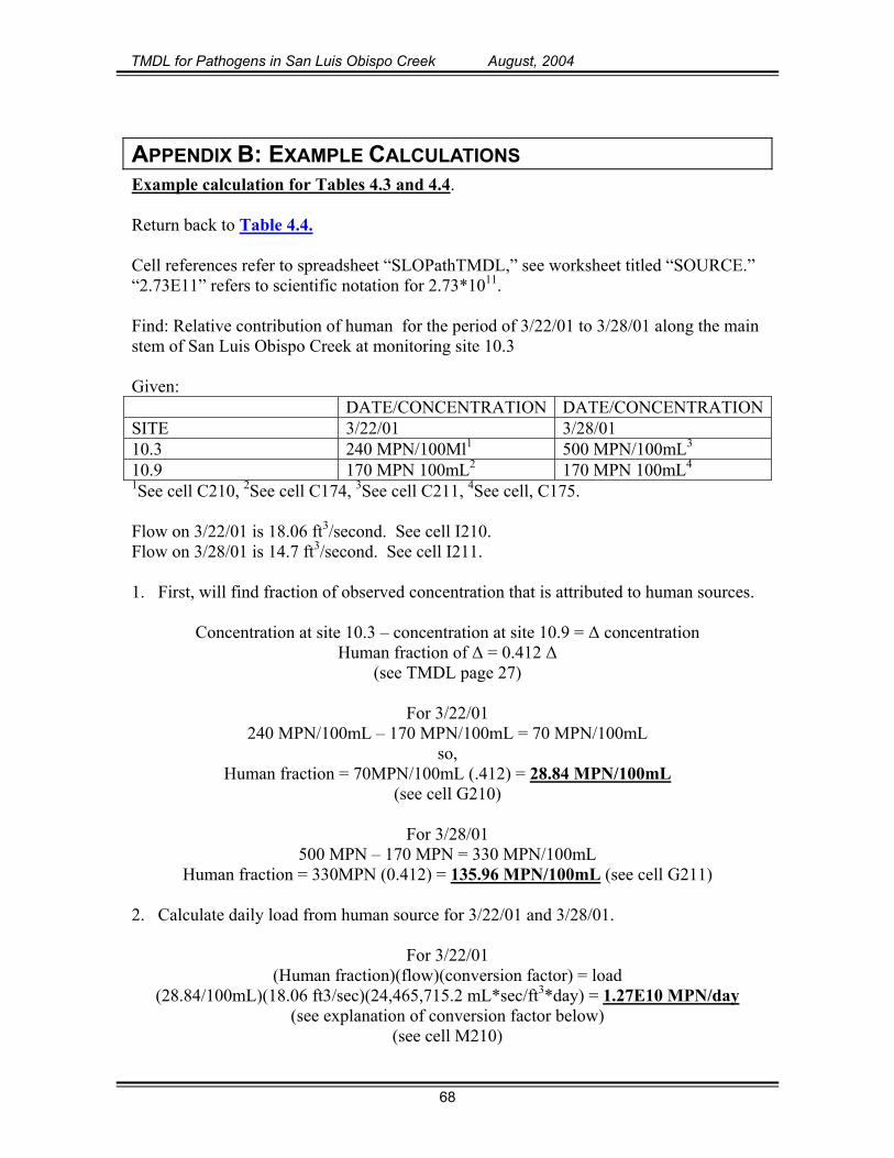
TMDL for Pathogens in San Luis Obispo Creek August, 2004
APPENDIX B: EXAMPLE CALCULATIONS Example calculation for Tables 4.3 and 4.4. Return back to Table 4.4. Cell references refer to spreadsheet “SLOPathTMDL,” see worksheet titled “SOURCE.” “2.73E11” refers to scientific notation for 2.73*1011. Find: Relative contribution of human for the period of 3/22/01 to 3/28/01 along the main stem of San Luis Obispo Creek at monitoring site 10.3 Given: DATE/CONCENTRATION DATE/CONCENTRATIONSITE 3/22/01 3/28/01 10.3 240 MPN/100Ml1 500 MPN/100mL3
10.9 170 MPN 100mL2 170 MPN 100mL4
1See cell C210, 2See cell C174, 3See cell C211, 4See cell, C175. Flow on 3/22/01 is 18.06 ft3/second. See cell I210. Flow on 3/28/01 is 14.7 ft /second. See cell I211. 3
1. First, will find fraction of observed concentration that is attributed to human sources.
Concentration at site 10.3 – concentration at site 10.9 = ∆ concentration Human fraction of ∆ = 0.412 ∆
(see TMDL page 27)
For 3/22/01 240 MPN/100mL – 170 MPN/100mL = 70 MPN/100mL
so, Human fraction = 70MPN/100mL (.412) = 28.84 MPN/100mL
(see cell G210)
For 3/28/01 500 MPN – 170 MPN = 330 MPN/100mL
Human fraction = 330MPN (0.412) = 135.96 MPN/100mL (see cell G211)
2. Calculate daily load from human source for 3/22/01 and 3/28/01.
For 3/22/01 (Human fraction)(flow)(conversion factor) = load
(28.84/100mL)(18.06 ft3/sec)(24,465,715.2 mL*sec/ft3*day) = 1.27E10 MPN/day (see explanation of conversion factor below)
(see cell M210)
68

TMDL for Pathogens in San Luis Obispo Creek August, 2004
For 3/28/01 (Human fraction)(flow)(conversion factor) = load
(135.96MPN/100mL)(14.7 ft3/sec)( 24,465,715.2 mL*sec/ft3*day)= 4.89E10 MPN/day (see cell M211)
Conversion Factor:
dayMPN
dayftmLftY
mLMPNX 2.715,465,24sec400,868.316,28
sec)(
100)(
3
3
=⋅⋅⋅
Substitute fecal coliform value (in MPN/100mL) for “X.” Substitute creek flow value (in ft3/sec) for “Y.” Result of calculation is in units of MPN/day.
3. Calculated the load from human for the period from 3/22/01 to 3/28/01
Area under graph is load
3/28/013/22/01
4.89E10 MPN/day 1.27E10 MPN/day
(1.27E10 MPN/day + 4.89E10 MPN/day)/2 * 6 days = 1.85E11 MPN (see cell T210)
4. Calculate the relative contribution of human during the period from 3/22/01 to 3/28/01.
ributionlativeContngTotalLoadi
mHumanLoadingFro Re%100 =
Total Loading (from all sources) shown in range of cells; D242 to H242. Background: 1.95E11 MPN; Based on 81MPN/100 mL and creek flow
Urban: 3.61E11 MPN; Calculated as the load left over after all other categories accounted Human: 1.85E11 MPN; Basis shown above.
TBB: 9.69E11MPN; Based on 21.6% ∆ (see TMDL page 27)
%30%10011)69.985.161.395.1(
1153.2=
+++ MPNEMPNE
Relative load contribution from human sources from 3/22/01 to 3/28/01 is 22%.
(see cell R242)
69

TMDL for Pathogens in San Luis Obispo Creek August, 2004
Example Calculation for Table 4.5 Return to Table 4.5 The relative contributions for each of the source categories in the main stem of San Luis Obispo Creek, located at monitoring site 10.0 (just downstream of the confluence with Stenner Creek) is shown in Table 4.5. The relative contribution for each source is the percent contribution of the sum of loading from Stenner Creek and the main stem of San Luis Obispo Creek upstream of the confluence with Stenner. The calculations are as follows:
Source
Main Stem Loading (lbs for the period
from 3/22/01-3/28/01)
Stenner Creek Loading (lbs for the
period from 3/22/01-3/28/01) Sum
Background (D267)1 1.95E11 1.95E11 3.90E11 Livestock (E267) 0 1.17E11 1.17E11 Urban (F267) 3.61E11 1.87E11 5.48E11 Human (G267) 1.85E11 0 1.85E11 TBB (H267) 9.69E10 0 9.69E10 Sum 8.37E11 4.99E11 1.34E12 1 Cell numbers refer to accompanying spreadsheet, SLOPathTMDL, worksheet “SOURCE.” Urban relative contribution (%) = Urban loading/Total Loading * 100%
%1001034.11048.5%89.40 12
11
×⋅⋅
= for period from 3/22/01 to 3/28/01
70

TMDL for Pathogens in San Luis Obispo Creek August, 2004
Example Calculation for Figure 4.6. Return to Figure 4.6. The relative loading in Table 4.5 is for ‘periods’ of time occurring between sampling days. However, the time periods are not equal. Therefore, in order to calculate the percentage of loading for the entire year of record for each source category, a weighted average was calculated based on the number of days in each period. The table below shows information from Table 4.5 for the Urban source category, then gives an example calculation for two time periods using the time weighted calculation, which in turn are used to determine the contribution from urban sources for the entire year of record. Refer to calculations in SLOPathTMDL spreadsheet, “SOURCE” worksheet, cell J295.
Period Period
from to
Days in period
Relative Contribution for Urban Source (from Table 4.5)
%
Time WeightedContribution for
Period %
Example Calculations
03/22/01 03/28/01 6 41a 0.34b .3441
7136
=⋅
03/28/01 04/06/01 9 42 0.52 52.42
7139
=⋅
04/06/01 04/13/01 7 36 0.35 “ 04/13/01 04/18/01 5 78 0.54 “ 04/18/01 05/18/01 30 62 2.62 “ 05/18/01 07/23/01 66 38 3.49 “ 07/23/01 09/13/01 52 40 2.93 “ 09/13/01 10/24/01 41 38 2.22 “ 10/24/01 11/15/01 22 29 0.90 “ 11/15/01 11/30/01 15 66 1.40 “ 11/30/01 01/14/02 45 56 3.50 “ 01/14/02 03/21/02 66 37 3.47 “ 03/21/02 04/23/02 33 37 1.73 “ 04/23/02 07/31/02 99 36 5.04 “ 07/31/02 09/18/02 49 35 2.42 “ 09/18/02 09/19/02 1 39 0.05 “ 09/19/02 11/27/02 69 65 6.26 “ 11/27/02 01/16/03 50 63 4.43 “ 01/16/03 03/05/03 48 60 4.07 “
Total Days = 713 Total Contribution (sum) = 46.3
(46%) Shown in Figure 4.6
a: shown in top row of data of Table 4.5 in Urban category. b: shown in SLOPathTMDL spreadsheet, worksheet “SOURCE” cell L295.
71

TMDL for Pathogens in San Luis Obispo Creek August, 2004
72