total variation in image analysis (the homo erectus stage?)
TRANSCRIPT
Total Variation
Total Variation in Image Analysis(The Homo Erectus Stage?)
François Lauze
1Department of Computer ScienceUniversity of Copenhagen
Hólar Summer School on Sparse Coding, August 2010
Total Variation
Outline
1 MotivationOrigin and uses of Total VariationDenoisingTikhonov regularization1-D computation on step edges
2 Total Variation IFirst definitionRudin-Osher-FatemiInpainting/Denoising
3 Total Variation IIRelaxing the derivative constraintsDefinition in actionUsing the new definition in denoising: Chambolle algorithmImage Simplification
4 Bibliography
5 The End
Total Variation
Motivation
Origin and uses of Total Variation
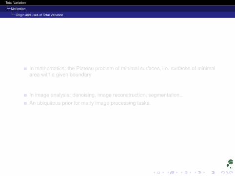
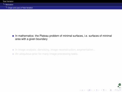
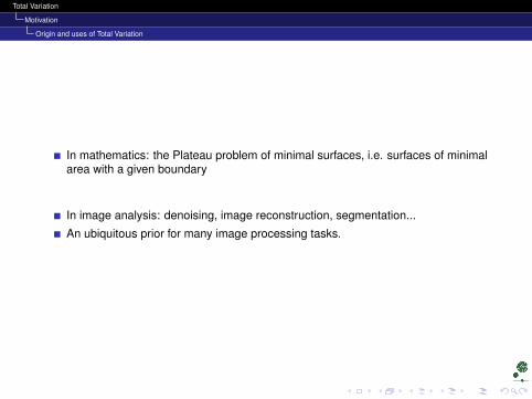
In mathematics: the Plateau problem of minimal surfaces, i.e. surfaces of minimalarea with a given boundary
In image analysis: denoising, image reconstruction, segmentation...
An ubiquitous prior for many image processing tasks.
Total Variation
Motivation
Origin and uses of Total Variation
In mathematics: the Plateau problem of minimal surfaces, i.e. surfaces of minimalarea with a given boundary
In image analysis: denoising, image reconstruction, segmentation...
An ubiquitous prior for many image processing tasks.
Total Variation
Motivation
Origin and uses of Total Variation
In mathematics: the Plateau problem of minimal surfaces, i.e. surfaces of minimalarea with a given boundary
In image analysis: denoising, image reconstruction, segmentation...
An ubiquitous prior for many image processing tasks.
Total Variation
Motivation
Denoising
Outline
1 MotivationOrigin and uses of Total VariationDenoisingTikhonov regularization1-D computation on step edges
2 Total Variation IFirst definitionRudin-Osher-FatemiInpainting/Denoising
3 Total Variation IIRelaxing the derivative constraintsDefinition in actionUsing the new definition in denoising: Chambolle algorithmImage Simplification
4 Bibliography
5 The End
Total Variation
Motivation
Denoising
Denoising
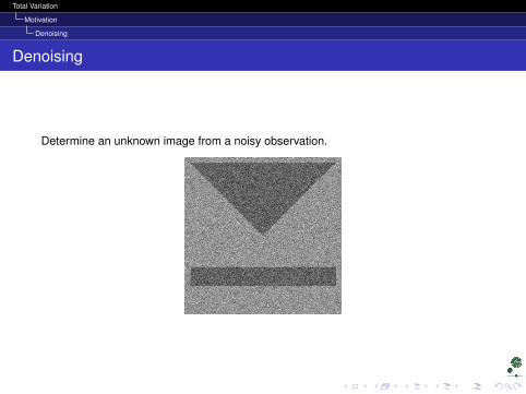
Determine an unknown image from a noisy observation.
Total Variation
Motivation
Denoising
Methods
All methods based on some statistical inference.
Fourier/Wavelets
Markov Random Fields
Variational and Partial Differential Equations methods
...
We focus on variational and PDE methods.
Total Variation
Motivation
Denoising
A simple corruption model
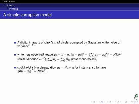
A digital image u of size N ×M pixels, corrupted by Gaussian white noise ofvariance σ2
write it as observed image u0 = u + η, ‖u − u0‖2 =∑
ij (uij − u0ij )2 = NMσ2
(noise variance = σ2),∑
ij uij =∑
ij u0ij (zero mean noise).
could add a blur degradation u0 = Ku + η for instance, so to have‖Ku − u0‖2 = NMσ2.
Total Variation
Motivation
Denoising
A simple corruption model
A digital image u of size N ×M pixels, corrupted by Gaussian white noise ofvariance σ2
write it as observed image u0 = u + η, ‖u − u0‖2 =∑
ij (uij − u0ij )2 = NMσ2
(noise variance = σ2),∑
ij uij =∑
ij u0ij (zero mean noise).
could add a blur degradation u0 = Ku + η for instance, so to have‖Ku − u0‖2 = NMσ2.
Total Variation
Motivation
Denoising
Recovery
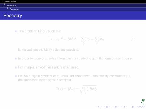
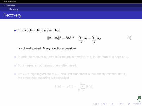
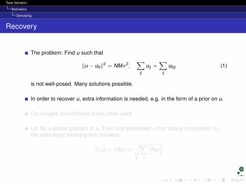
The problem: Find u such that
‖u − u0‖2 = NMσ2,∑
ij
uij =∑
ij
u0ij (1)
is not well-posed. Many solutions possible.
In order to recover u, extra information is needed, e.g. in the form of a prior on u.
For images, smoothness priors often used.
Let Ru a digital gradient of u, Then find smoothest u that satisfy constraints (1),the smoothest meaning with smallest
T (u) = ‖Ru‖ =
√∑ij
|Ru|2ij .
Total Variation
Motivation
Denoising
Recovery
The problem: Find u such that
‖u − u0‖2 = NMσ2,∑
ij
uij =∑
ij
u0ij (1)
is not well-posed. Many solutions possible.
In order to recover u, extra information is needed, e.g. in the form of a prior on u.
For images, smoothness priors often used.
Let Ru a digital gradient of u, Then find smoothest u that satisfy constraints (1),the smoothest meaning with smallest
T (u) = ‖Ru‖ =
√∑ij
|Ru|2ij .
Total Variation
Motivation
Tikhonov regularization
Outline
1 MotivationOrigin and uses of Total VariationDenoisingTikhonov regularization1-D computation on step edges
2 Total Variation IFirst definitionRudin-Osher-FatemiInpainting/Denoising
3 Total Variation IIRelaxing the derivative constraintsDefinition in actionUsing the new definition in denoising: Chambolle algorithmImage Simplification
4 Bibliography
5 The End
Total Variation
Motivation
Tikhonov regularization
Tikhonov regularization
It can be show that this is equivalent to minimize
E(u) = ‖Ku − u0‖2 + λ‖Ru‖2
for a λ = λ(σ) (Wahba?).
E(u) minimizaton can be derived from a Maximum a Posteriori formulation
Arg.maxu
p(u|u0) =p(u0|u)p(u)
p(u0)
Rewriting in a continuous setting:
E(u) =
∫Ω
(Ku − uo)2 dx + λ
∫Ω|∇u|2 dx
Total Variation
Motivation
Tikhonov regularization
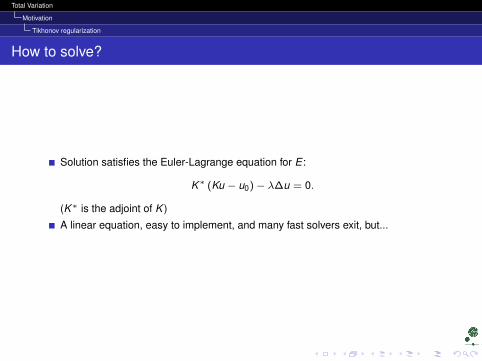
How to solve?
Solution satisfies the Euler-Lagrange equation for E :
K∗ (Ku − u0)− λ∆u = 0.
(K∗ is the adjoint of K )
A linear equation, easy to implement, and many fast solvers exit, but...
Total Variation
Motivation
Tikhonov regularization
How to solve?
Solution satisfies the Euler-Lagrange equation for E :
K∗ (Ku − u0)− λ∆u = 0.
(K∗ is the adjoint of K )
A linear equation, easy to implement, and many fast solvers exit, but...
Total Variation
Motivation
Tikhonov regularization
How to solve?
Solution satisfies the Euler-Lagrange equation for E :
K∗ (Ku − u0)− λ∆u = 0.
(K∗ is the adjoint of K )
A linear equation, easy to implement, and many fast solvers exit, but...
Total Variation
Motivation
Tikhonov regularization
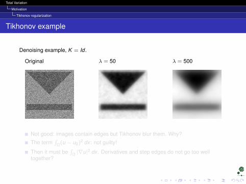
Tikhonov example
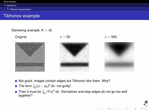
Denoising example, K = Id .
Original λ = 50 λ = 500
Not good: images contain edges but Tikhonov blur them. Why?
The term∫
Ω(u − u0)2 dx : not guilty!
Then it must be∫
Ω |∇u|2 dx . Derivatives and step edges do not go too welltogether?
Total Variation
Motivation
Tikhonov regularization
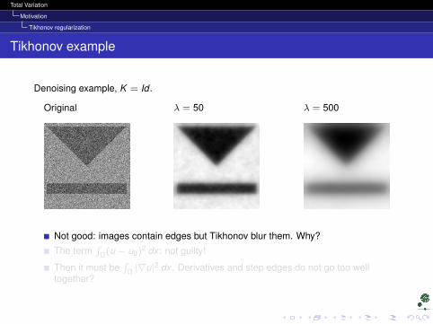
Tikhonov example
Denoising example, K = Id .
Original λ = 50 λ = 500
Not good: images contain edges but Tikhonov blur them. Why?
The term∫
Ω(u − u0)2 dx : not guilty!
Then it must be∫
Ω |∇u|2 dx . Derivatives and step edges do not go too welltogether?
Total Variation
Motivation
Tikhonov regularization
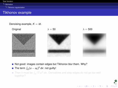
Tikhonov example
Denoising example, K = Id .
Original λ = 50 λ = 500
Not good: images contain edges but Tikhonov blur them. Why?
The term∫
Ω(u − u0)2 dx : not guilty!
Then it must be∫
Ω |∇u|2 dx . Derivatives and step edges do not go too welltogether?
Total Variation
Motivation
Tikhonov regularization
Tikhonov example
Denoising example, K = Id .
Original λ = 50 λ = 500
Not good: images contain edges but Tikhonov blur them. Why?
The term∫
Ω(u − u0)2 dx : not guilty!
Then it must be∫
Ω |∇u|2 dx . Derivatives and step edges do not go too welltogether?
Total Variation
Motivation
1-D computation on step edges
Outline
1 MotivationOrigin and uses of Total VariationDenoisingTikhonov regularization1-D computation on step edges
2 Total Variation IFirst definitionRudin-Osher-FatemiInpainting/Denoising
3 Total Variation IIRelaxing the derivative constraintsDefinition in actionUsing the new definition in denoising: Chambolle algorithmImage Simplification
4 Bibliography
5 The End
Total Variation
Motivation
1-D computation on step edges
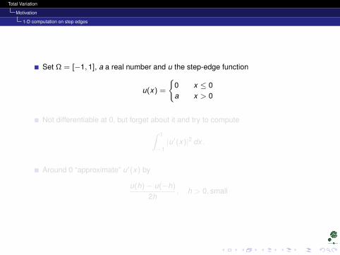
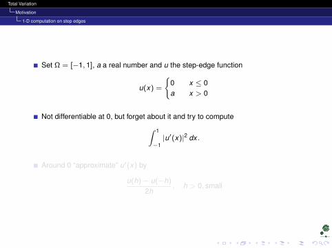
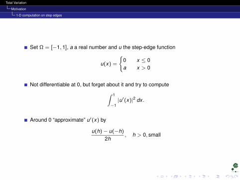
Set Ω = [−1, 1], a a real number and u the step-edge function
u(x) =
0 x ≤ 0a x > 0
Not differentiable at 0, but forget about it and try to compute∫ 1
−1|u′(x)|2 dx .
Around 0 “approximate” u′(x) by
u(h)− u(−h)
2h, h > 0, small
Total Variation
Motivation
1-D computation on step edges
Set Ω = [−1, 1], a a real number and u the step-edge function
u(x) =
0 x ≤ 0a x > 0
Not differentiable at 0, but forget about it and try to compute∫ 1
−1|u′(x)|2 dx .
Around 0 “approximate” u′(x) by
u(h)− u(−h)
2h, h > 0, small
Total Variation
Motivation
1-D computation on step edges
Set Ω = [−1, 1], a a real number and u the step-edge function
u(x) =
0 x ≤ 0a x > 0
Not differentiable at 0, but forget about it and try to compute∫ 1
−1|u′(x)|2 dx .
Around 0 “approximate” u′(x) by
u(h)− u(−h)
2h, h > 0, small
Total Variation
Motivation
1-D computation on step edges
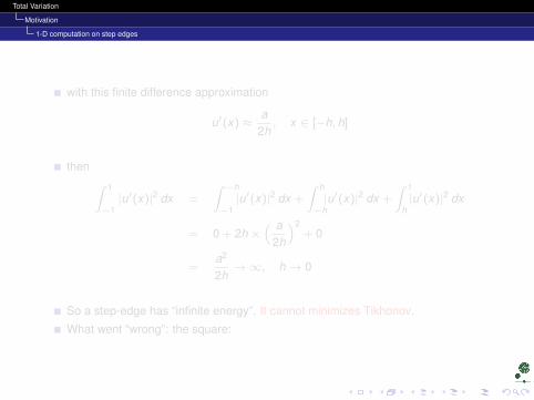
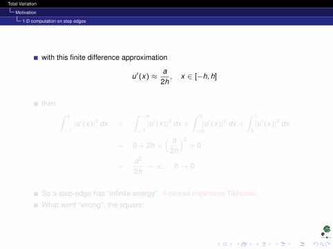
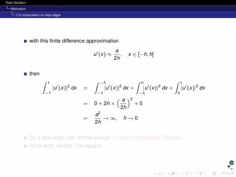
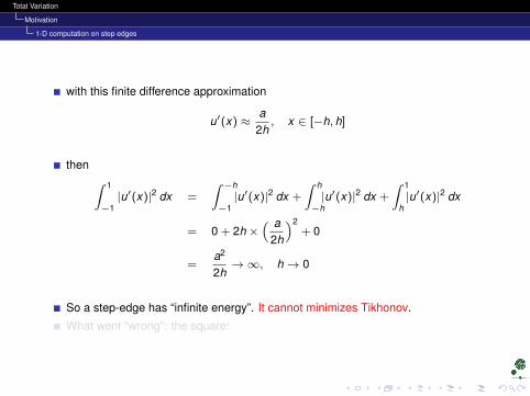
with this finite difference approximation
u′(x) ≈a
2h, x ∈ [−h, h]
then ∫ 1
−1|u′(x)|2 dx =
∫ −h
−1|u′(x)|2 dx +
∫ h
−h|u′(x)|2 dx +
∫ 1
h|u′(x)|2 dx
= 0 + 2h ×( a
2h
)2+ 0
=a2
2h→∞, h→ 0
So a step-edge has “infinite energy”. It cannot minimizes Tikhonov.
What went “wrong”: the square:
Total Variation
Motivation
1-D computation on step edges
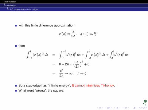
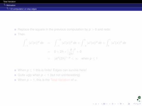
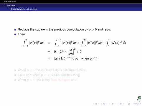
Replace the square in the previous computation by p > 0 and redo:
Then∫ 1
−1|u′(x)|p dx =
∫ −h
−1|u′(x)|p dx +
∫ h
−h|u′(x)|p dx +
∫ 1
h|u′(x)|p dx
= 0 + 2h ×∣∣∣ a2h
∣∣∣p + 0
= |a|p(2h)1−p <∞ when p ≤ 1
When p ≤ 1 this is finite! Edges can survive here!
Quite ugly when p < 1 (but not uninteresting)
When p = 1, this is the Total Variation of u.
Total Variation
Motivation
1-D computation on step edges
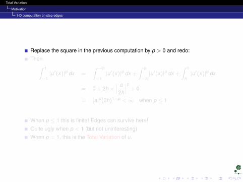
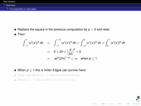
Replace the square in the previous computation by p > 0 and redo:
Then∫ 1
−1|u′(x)|p dx =
∫ −h
−1|u′(x)|p dx +
∫ h
−h|u′(x)|p dx +
∫ 1
h|u′(x)|p dx
= 0 + 2h ×∣∣∣ a2h
∣∣∣p + 0
= |a|p(2h)1−p <∞ when p ≤ 1
When p ≤ 1 this is finite! Edges can survive here!
Quite ugly when p < 1 (but not uninteresting)
When p = 1, this is the Total Variation of u.
Total Variation
Motivation
1-D computation on step edges
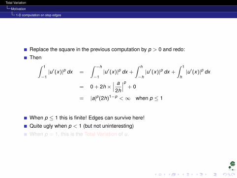
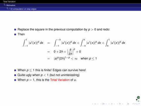
Replace the square in the previous computation by p > 0 and redo:
Then∫ 1
−1|u′(x)|p dx =
∫ −h
−1|u′(x)|p dx +
∫ h
−h|u′(x)|p dx +
∫ 1
h|u′(x)|p dx
= 0 + 2h ×∣∣∣ a2h
∣∣∣p + 0
= |a|p(2h)1−p <∞ when p ≤ 1
When p ≤ 1 this is finite! Edges can survive here!
Quite ugly when p < 1 (but not uninteresting)
When p = 1, this is the Total Variation of u.
Total Variation
Total Variation I
First definition
Outline
1 MotivationOrigin and uses of Total VariationDenoisingTikhonov regularization1-D computation on step edges
2 Total Variation IFirst definitionRudin-Osher-FatemiInpainting/Denoising
3 Total Variation IIRelaxing the derivative constraintsDefinition in actionUsing the new definition in denoising: Chambolle algorithmImage Simplification
4 Bibliography
5 The End
Total Variation
Total Variation I
First definition
Let u : Ω ⊂ Rn → R. Define total variation as
J(u) =
∫Ω|∇u| dx , |∇u| =
√√√√ n∑i=1
u2xi.
When J(u) is finite, one says that u has bounded variations and the space offunction of bounded variations on Ω is denoted BV (Ω).
Total Variation
Total Variation I
First definition
Let u : Ω ⊂ Rn → R. Define total variation as
J(u) =
∫Ω|∇u| dx , |∇u| =
√√√√ n∑i=1
u2xi.
When J(u) is finite, one says that u has bounded variations and the space offunction of bounded variations on Ω is denoted BV (Ω).
Total Variation
Total Variation I
First definition
Expected: when minimizing J(u) with other constraints, edges are less penalizedthat with Tikhonov.
Indeed edges are “naturally present” in bounded variation functions. In fact:functions of bounded variations can be decomposed in
1 smooth parts,∇u well defined,
2 Jump discontinuities (our edges)
3 something else (Cantor part) which can be nasty...
The functions that do not possess this nasty part form a subspace of BV (Ω)called SBV (Ω), The Special functions of Bounded Variation, (used for instancewhen studying Mumford-Shah functional)
Total Variation
Total Variation I
Rudin-Osher-Fatemi
Outline
1 MotivationOrigin and uses of Total VariationDenoisingTikhonov regularization1-D computation on step edges
2 Total Variation IFirst definitionRudin-Osher-FatemiInpainting/Denoising
3 Total Variation IIRelaxing the derivative constraintsDefinition in actionUsing the new definition in denoising: Chambolle algorithmImage Simplification
4 Bibliography
5 The End
Total Variation
Total Variation I
Rudin-Osher-Fatemi
ROF Denoising
State the denoising problem as minimizing J(u) under the constraints∫Ω
u dx =
∫Ω
uo dx ,∫
Ω(u − u0)2 dx = |Ω|σ2 (|Ω| = area/volume of Ω)
Solve via Lagrange multipliers.
Total Variation
Total Variation I
Rudin-Osher-Fatemi
ROF Denoising
State the denoising problem as minimizing J(u) under the constraints∫Ω
u dx =
∫Ω
uo dx ,∫
Ω(u − u0)2 dx = |Ω|σ2 (|Ω| = area/volume of Ω)
Solve via Lagrange multipliers.
Total Variation
Total Variation I
Rudin-Osher-Fatemi
ROF Denoising
State the denoising problem as minimizing J(u) under the constraints∫Ω
u dx =
∫Ω
uo dx ,∫
Ω(u − u0)2 dx = |Ω|σ2 (|Ω| = area/volume of Ω)
Solve via Lagrange multipliers.
Total Variation
Total Variation I
Rudin-Osher-Fatemi
TV-denoising
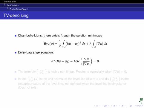
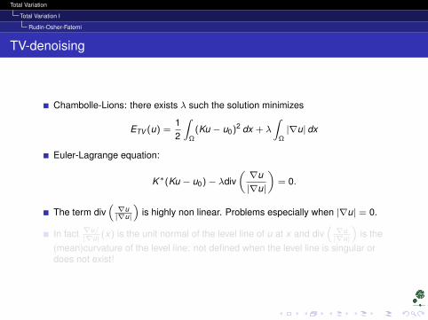
Chambolle-Lions: there exists λ such the solution minimizes
ETV (u) =12
∫Ω
(Ku − u0)2 dx + λ
∫Ω|∇u| dx
Euler-Lagrange equation:
K∗(Ku − u0)− λdiv(∇u|∇u|
)= 0.
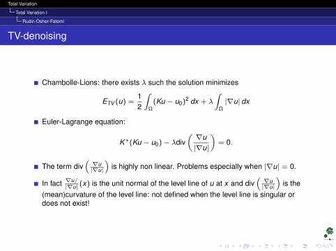
The term div(∇u|∇u|
)is highly non linear. Problems especially when |∇u| = 0.
In fact ∇u/|∇u| (x) is the unit normal of the level line of u at x and div
(∇u|∇u|
)is the
(mean)curvature of the level line: not defined when the level line is singular ordoes not exist!
Total Variation
Total Variation I
Rudin-Osher-Fatemi
TV-denoising
Chambolle-Lions: there exists λ such the solution minimizes
ETV (u) =12
∫Ω
(Ku − u0)2 dx + λ
∫Ω|∇u| dx
Euler-Lagrange equation:
K∗(Ku − u0)− λdiv(∇u|∇u|
)= 0.
The term div(∇u|∇u|
)is highly non linear. Problems especially when |∇u| = 0.
In fact ∇u/|∇u| (x) is the unit normal of the level line of u at x and div
(∇u|∇u|
)is the
(mean)curvature of the level line: not defined when the level line is singular ordoes not exist!
Total Variation
Total Variation I
Rudin-Osher-Fatemi
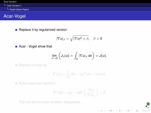
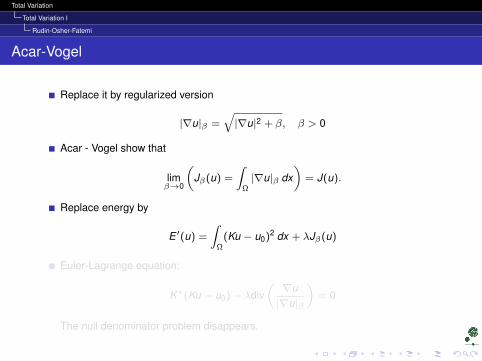
Acar-Vogel
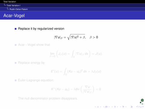
Replace it by regularized version
|∇u|β =√|∇u|2 + β, β > 0
Acar - Vogel show that
limβ→0
(Jβ(u) =
∫Ω|∇u|β dx
)= J(u).
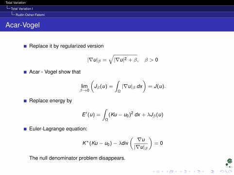
Replace energy by
E ′(u) =
∫Ω
(Ku − u0)2 dx + λJβ(u)
Euler-Lagrange equation:
K∗(Ku − u0)− λdiv(∇u|∇u|β
)= 0
The null denominator problem disappears.
Total Variation
Total Variation I
Rudin-Osher-Fatemi
Acar-Vogel
Replace it by regularized version
|∇u|β =√|∇u|2 + β, β > 0
Acar - Vogel show that
limβ→0
(Jβ(u) =
∫Ω|∇u|β dx
)= J(u).
Replace energy by
E ′(u) =
∫Ω
(Ku − u0)2 dx + λJβ(u)
Euler-Lagrange equation:
K∗(Ku − u0)− λdiv(∇u|∇u|β
)= 0
The null denominator problem disappears.

Total Variation
Total Variation I
Rudin-Osher-Fatemi
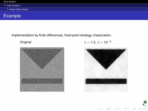
Example
Implementation by finite differences, fixed-point strategy, linearization.
Original λ = 1.5, β = 10−4
Total Variation
Total Variation I
Rudin-Osher-Fatemi
Example
Implementation by finite differences, fixed-point strategy, linearization.
Original λ = 1.5, β = 10−4
Total Variation
Total Variation I
Inpainting/Denoising
Outline
1 MotivationOrigin and uses of Total VariationDenoisingTikhonov regularization1-D computation on step edges
2 Total Variation IFirst definitionRudin-Osher-FatemiInpainting/Denoising
3 Total Variation IIRelaxing the derivative constraintsDefinition in actionUsing the new definition in denoising: Chambolle algorithmImage Simplification
4 Bibliography
5 The End
Total Variation
Total Variation I
Inpainting/Denoising
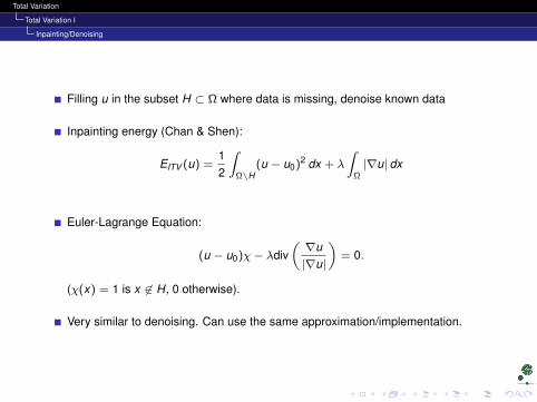
Filling u in the subset H ⊂ Ω where data is missing, denoise known data
Inpainting energy (Chan & Shen):
EITV (u) =12
∫Ω\H
(u − u0)2 dx + λ
∫Ω|∇u| dx
Euler-Lagrange Equation:
(u − u0)χ− λdiv(∇u|∇u|
)= 0.
(χ(x) = 1 is x 6∈ H, 0 otherwise).
Very similar to denoising. Can use the same approximation/implementation.
Total Variation
Total Variation I
Inpainting/Denoising
Filling u in the subset H ⊂ Ω where data is missing, denoise known data
Inpainting energy (Chan & Shen):
EITV (u) =12
∫Ω\H
(u − u0)2 dx + λ
∫Ω|∇u| dx
Euler-Lagrange Equation:
(u − u0)χ− λdiv(∇u|∇u|
)= 0.
(χ(x) = 1 is x 6∈ H, 0 otherwise).
Very similar to denoising. Can use the same approximation/implementation.
Total Variation
Total Variation I
Inpainting/Denoising
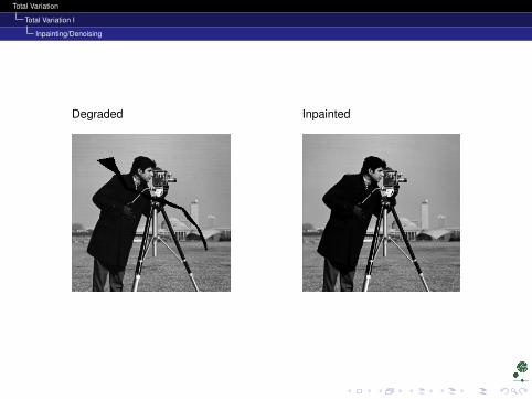
Degraded Inpainted
Total Variation
Total Variation I
Inpainting/Denoising
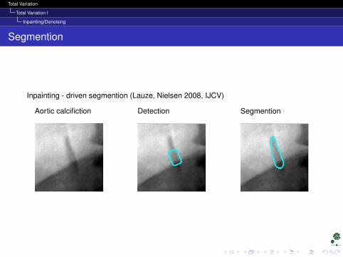
Segmention
Inpainting - driven segmention (Lauze, Nielsen 2008, IJCV)
Aortic calcifiction Detection Segmention
Total Variation
Total Variation II
Relaxing the derivative constraints
Outline
1 MotivationOrigin and uses of Total VariationDenoisingTikhonov regularization1-D computation on step edges
2 Total Variation IFirst definitionRudin-Osher-FatemiInpainting/Denoising
3 Total Variation IIRelaxing the derivative constraintsDefinition in actionUsing the new definition in denoising: Chambolle algorithmImage Simplification
4 Bibliography
5 The End
Total Variation
Total Variation II
Relaxing the derivative constraints
With definition of total variation as
J(u) =
∫Ω|∇u| dx
u must have (weak) derivatives.
But we just saw that the computation is possible for a step-edge u(x) = 0, x < 0,u(x) = a, x > 0: ∫ 1
−1|u′(x)| dx = |a|
Can we avoid the use of derivatives of u?
Total Variation
Total Variation II
Relaxing the derivative constraints
Assume first that ∇u exists.
|∇u| = ∇u ·∇u|∇u|
(except when ∇u = 0) and ∇u|∇u| is the normal to the level lines of u, it has
everywhere norm 1.
Let V the set of vector fields v(x) on Ω with |v(x)| ≤ 1. I claim
J(u) = supv∈V
∫Ω∇u(x) · v(x) dx
(consequence of Cauchy-Schwarz inequality).
Total Variation
Total Variation II
Relaxing the derivative constraints
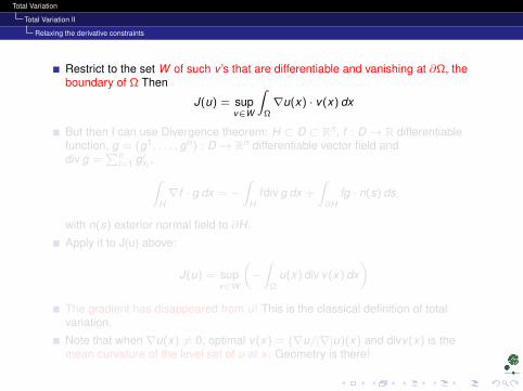
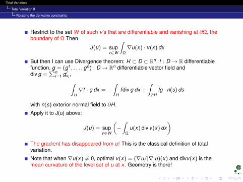
Restrict to the set W of such v ’s that are differentiable and vanishing at ∂Ω, theboundary of Ω Then
J(u) = supv∈W
∫Ω∇u(x) · v(x) dx
But then I can use Divergence theorem: H ⊂ D ⊂ Rn, f : D → R differentiablefunction, g = (g1, . . . , gn) : D → Rn differentiable vector field anddiv g =
∑ni=1 g i
xi,∫
H∇f · g dx = −
∫H
fdiv g dx +
∫∂H
fg · n(s) ds
with n(s) exterior normal field to ∂H.
Apply it to J(u) above:
J(u) = supv∈W
(−∫
Ωu(x) div v(x) dx
)The gradient has disappeared from u! This is the classical definition of totalvariation.
Note that when ∇u(x) 6= 0, optimal v(x) = (∇u/|∇|u)(x) and divv(x) is themean curvature of the level set of u at x . Geometry is there!
Total Variation
Total Variation II
Relaxing the derivative constraints
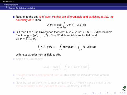
Restrict to the set W of such v ’s that are differentiable and vanishing at ∂Ω, theboundary of Ω Then
J(u) = supv∈W
∫Ω∇u(x) · v(x) dx
But then I can use Divergence theorem: H ⊂ D ⊂ Rn, f : D → R differentiablefunction, g = (g1, . . . , gn) : D → Rn differentiable vector field anddiv g =
∑ni=1 g i
xi,∫
H∇f · g dx = −
∫H
fdiv g dx +
∫∂H
fg · n(s) ds
with n(s) exterior normal field to ∂H.
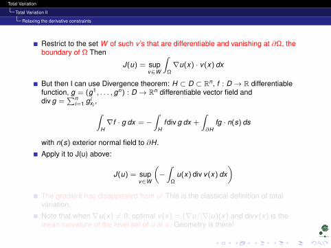
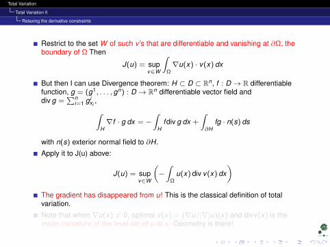
Apply it to J(u) above:
J(u) = supv∈W
(−∫
Ωu(x) div v(x) dx
)The gradient has disappeared from u! This is the classical definition of totalvariation.
Note that when ∇u(x) 6= 0, optimal v(x) = (∇u/|∇|u)(x) and divv(x) is themean curvature of the level set of u at x . Geometry is there!
Total Variation
Total Variation II
Relaxing the derivative constraints
Restrict to the set W of such v ’s that are differentiable and vanishing at ∂Ω, theboundary of Ω Then
J(u) = supv∈W
∫Ω∇u(x) · v(x) dx
But then I can use Divergence theorem: H ⊂ D ⊂ Rn, f : D → R differentiablefunction, g = (g1, . . . , gn) : D → Rn differentiable vector field anddiv g =
∑ni=1 g i
xi,∫
H∇f · g dx = −
∫H
fdiv g dx +
∫∂H
fg · n(s) ds
with n(s) exterior normal field to ∂H.
Apply it to J(u) above:
J(u) = supv∈W
(−∫
Ωu(x) div v(x) dx
)The gradient has disappeared from u! This is the classical definition of totalvariation.
Note that when ∇u(x) 6= 0, optimal v(x) = (∇u/|∇|u)(x) and divv(x) is themean curvature of the level set of u at x . Geometry is there!
Total Variation
Total Variation II
Definition in action
Outline
1 MotivationOrigin and uses of Total VariationDenoisingTikhonov regularization1-D computation on step edges
2 Total Variation IFirst definitionRudin-Osher-FatemiInpainting/Denoising
3 Total Variation IIRelaxing the derivative constraintsDefinition in actionUsing the new definition in denoising: Chambolle algorithmImage Simplification
4 Bibliography
5 The End
Total Variation
Total Variation II
Definition in action
Step-edge
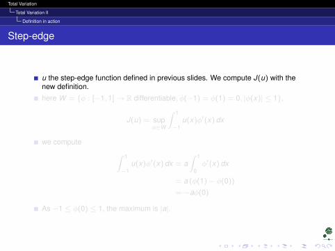
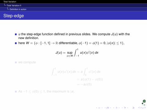
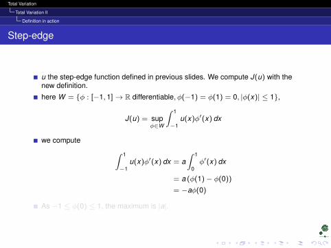
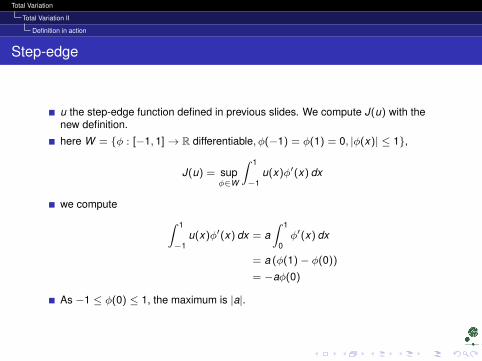
u the step-edge function defined in previous slides. We compute J(u) with thenew definition.
here W = φ : [−1, 1]→ R differentiable, φ(−1) = φ(1) = 0, |φ(x)| ≤ 1,
J(u) = supφ∈W
∫ 1
−1u(x)φ′(x) dx
we compute ∫ 1
−1u(x)φ′(x) dx = a
∫ 1
0φ′(x) dx
= a (φ(1)− φ(0))
= −aφ(0)
As −1 ≤ φ(0) ≤ 1, the maximum is |a|.
Total Variation
Total Variation II
Definition in action
Step-edge
u the step-edge function defined in previous slides. We compute J(u) with thenew definition.
here W = φ : [−1, 1]→ R differentiable, φ(−1) = φ(1) = 0, |φ(x)| ≤ 1,
J(u) = supφ∈W
∫ 1
−1u(x)φ′(x) dx
we compute ∫ 1
−1u(x)φ′(x) dx = a
∫ 1
0φ′(x) dx
= a (φ(1)− φ(0))
= −aφ(0)
As −1 ≤ φ(0) ≤ 1, the maximum is |a|.
Total Variation
Total Variation II
Definition in action
2D example
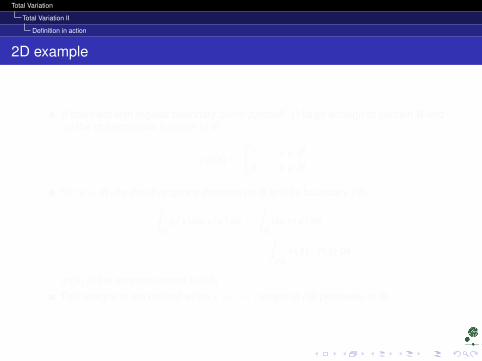
B open set with regular boundary curve partialB, Ω large enough to contain B andχB the characteristic function of B
χB(x) =
1 x ∈ B0 x 6∈ B
For v ∈ W , by the divergence theorem on B and its boundary ∂B∫Ωχ(x)div v(x) dx =
∫B
div v(x) dx
= −∫∂B
v(s) · n(s) ds
(n(s) is the exterior normal to ∂B)
This integral is maximized when v = −n : length of ∂B perimeter of B.
Total Variation
Total Variation II
Definition in action
2D example
B open set with regular boundary curve partialB, Ω large enough to contain B andχB the characteristic function of B
χB(x) =
1 x ∈ B0 x 6∈ B
For v ∈ W , by the divergence theorem on B and its boundary ∂B∫Ωχ(x)div v(x) dx =
∫B
div v(x) dx
= −∫∂B
v(s) · n(s) ds
(n(s) is the exterior normal to ∂B)
This integral is maximized when v = −n : length of ∂B perimeter of B.
Total Variation
Total Variation II
Definition in action
Sets of finite perimeter
Let H ⊂ Ω. If its characteristic function χH satisfies
J(χH ) <∞
H is called set of finite perimeter (and PerΩ(H) := J(χH ) is its perimeter)
This is used for instance in the Chan and Vese algorithm.
If J(u) <∞ and Ht = x ∈ Ω, u(x) < t the lower t-level set of u,
J(u) =
∫ +∞
−∞J(χHt ) dt Coarea formula
Total Variation
Total Variation II
Using the new definition in denoising: Chambolle algorithm
Outline
1 MotivationOrigin and uses of Total VariationDenoisingTikhonov regularization1-D computation on step edges
2 Total Variation IFirst definitionRudin-Osher-FatemiInpainting/Denoising
3 Total Variation IIRelaxing the derivative constraintsDefinition in actionUsing the new definition in denoising: Chambolle algorithmImage Simplification
4 Bibliography
5 The End
Total Variation
Total Variation II
Using the new definition in denoising: Chambolle algorithm
Chambolle algorithm
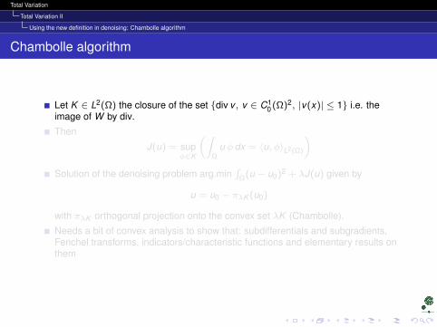
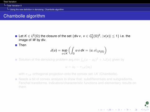
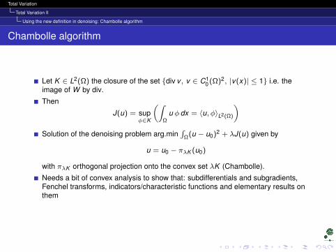
Let K ∈ L2(Ω) the closure of the set div v , v ∈ C10 (Ω)2, |v(x)| ≤ 1 i.e. the
image of W by div.
Then
J(u) = supφ∈K
(∫Ω
u φ dx = 〈u, φ〉L2(Ω)
)Solution of the denoising problem arg.min
∫Ω(u − u0)2 + λJ(u) given by
u = u0 − πλK (u0)
with πλK orthogonal projection onto the convex set λK (Chambolle).
Needs a bit of convex analysis to show that: subdifferentials and subgradients,Fenchel transforms, indicators/characteristic functions and elementary results onthem
Total Variation
Total Variation II
Using the new definition in denoising: Chambolle algorithm
Chambolle algorithm
Let K ∈ L2(Ω) the closure of the set div v , v ∈ C10 (Ω)2, |v(x)| ≤ 1 i.e. the
image of W by div.
Then
J(u) = supφ∈K
(∫Ω
u φ dx = 〈u, φ〉L2(Ω)
)Solution of the denoising problem arg.min
∫Ω(u − u0)2 + λJ(u) given by
u = u0 − πλK (u0)
with πλK orthogonal projection onto the convex set λK (Chambolle).
Needs a bit of convex analysis to show that: subdifferentials and subgradients,Fenchel transforms, indicators/characteristic functions and elementary results onthem
Total Variation
Total Variation II
Using the new definition in denoising: Chambolle algorithm
Fenchel Transform
X Hilbert space, f : X → R convex, proper. Fenchel transform of F :
F∗(v) = supu∈X
(〈u, v〉X − F (u))
Geometric meaning: take u∗ such that F∗(u∗) < +∞: the affine function
a(u) = 〈u, u∗〉 − F∗(u∗)
is tangent to F and a(0) = −F∗(u∗).
Total Variation
Total Variation II
Using the new definition in denoising: Chambolle algorithm
Fenchel transform
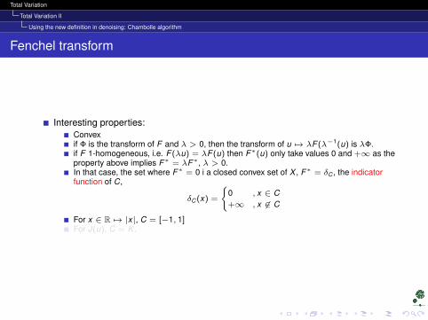
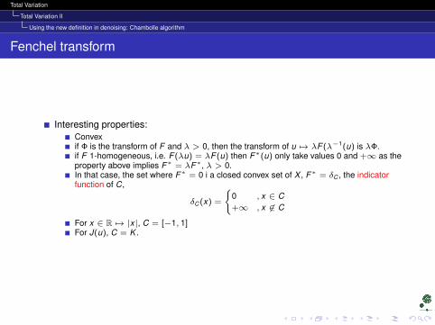
Interesting properties:Convexif Φ is the transform of F and λ > 0, then the transform of u 7→ λF (λ−1(u) is λΦ.if F 1-homogeneous, i.e. F (λu) = λF (u) then F∗(u) only take values 0 and +∞ as theproperty above implies F∗ = λF∗, λ > 0.In that case, the set where F∗ = 0 i a closed convex set of X , F∗ = δC , the indicatorfunction of C,
δC (x) =
0 , x ∈ C+∞ , x 6∈ C
For x ∈ R 7→ |x|, C = [−1, 1]For J(u), C = K .
Total Variation
Total Variation II
Using the new definition in denoising: Chambolle algorithm
Fenchel transform
Interesting properties:Convexif Φ is the transform of F and λ > 0, then the transform of u 7→ λF (λ−1(u) is λΦ.if F 1-homogeneous, i.e. F (λu) = λF (u) then F∗(u) only take values 0 and +∞ as theproperty above implies F∗ = λF∗, λ > 0.In that case, the set where F∗ = 0 i a closed convex set of X , F∗ = δC , the indicatorfunction of C,
δC (x) =
0 , x ∈ C+∞ , x 6∈ C
For x ∈ R 7→ |x|, C = [−1, 1]For J(u), C = K .
Total Variation
Total Variation II
Using the new definition in denoising: Chambolle algorithm
Subdifferentials
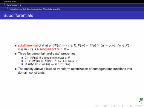
subdifferential of F at u: ∂F (u) = v ∈ X ,F (w)− F (u) ≥ 〈w − u, v〉, ∀w ∈ X.v ∈ ∂F (u) is a subgradient of F at u.Three fundamental (and easy) properties:
0 ∈ ∂F (u) iff u global minimizer of Fu∗ ∈ ∂F (u)⇔ F (u) + F∗(u∗) = 〈u, u∗〉Duality: u∗ ∈ ∂F (u)⇔ u ∈ ∂F∗(u)
The duality above allows to transform optimization of homogeneous functions intodomain constraints!
Total Variation
Total Variation II
Using the new definition in denoising: Chambolle algorithm
Subdifferentials
subdifferential of F at u: ∂F (u) = v ∈ X ,F (w)− F (u) ≥ 〈w − u, v〉, ∀w ∈ X.v ∈ ∂F (u) is a subgradient of F at u.Three fundamental (and easy) properties:
0 ∈ ∂F (u) iff u global minimizer of Fu∗ ∈ ∂F (u)⇔ F (u) + F∗(u∗) = 〈u, u∗〉Duality: u∗ ∈ ∂F (u)⇔ u ∈ ∂F∗(u)
The duality above allows to transform optimization of homogeneous functions intodomain constraints!
Total Variation
Total Variation II
Using the new definition in denoising: Chambolle algorithm
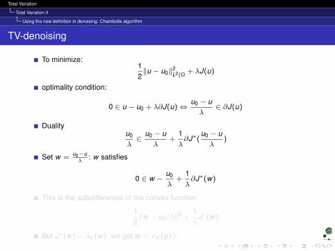
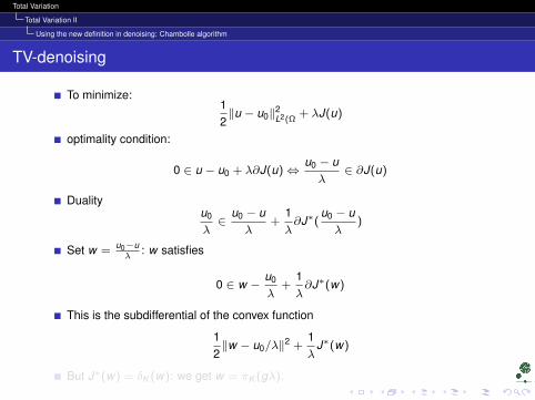
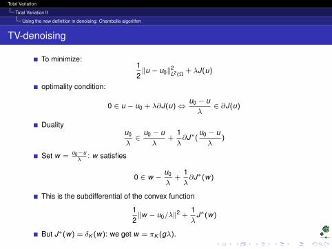
TV-denoising
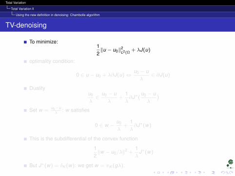
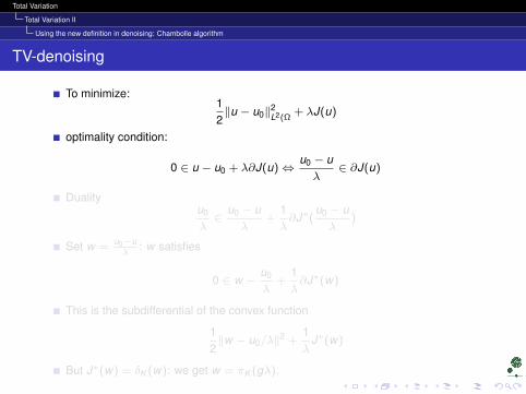
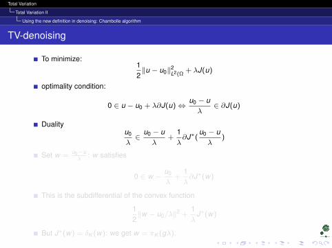
To minimize:12‖u − u0‖2
L2(Ω+ λJ(u)
optimality condition:
0 ∈ u − u0 + λ∂J(u)⇔u0 − uλ
∈ ∂J(u)
Dualityu0
λ∈
u0 − uλ
+1λ∂J∗(
u0 − uλ
)
Set w =u0−uλ
: w satisfies
0 ∈ w −u0
λ+
1λ∂J∗(w)
This is the subdifferential of the convex function
12‖w − u0/λ‖2 +
1λ
J∗(w)
But J∗(w) = δK (w): we get w = πK (gλ).
Total Variation
Total Variation II
Using the new definition in denoising: Chambolle algorithm
TV-denoising
To minimize:12‖u − u0‖2
L2(Ω+ λJ(u)
optimality condition:
0 ∈ u − u0 + λ∂J(u)⇔u0 − uλ
∈ ∂J(u)
Dualityu0
λ∈
u0 − uλ
+1λ∂J∗(
u0 − uλ
)
Set w =u0−uλ
: w satisfies
0 ∈ w −u0
λ+
1λ∂J∗(w)
This is the subdifferential of the convex function
12‖w − u0/λ‖2 +
1λ
J∗(w)
But J∗(w) = δK (w): we get w = πK (gλ).
Total Variation
Total Variation II
Using the new definition in denoising: Chambolle algorithm
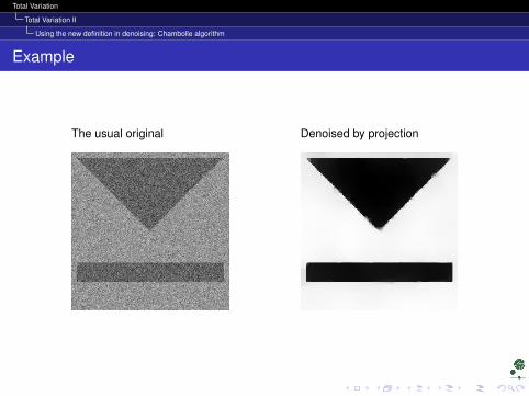
Example
The usual original Denoised by projection
Total Variation
Total Variation II
Image Simplification
Outline
1 MotivationOrigin and uses of Total VariationDenoisingTikhonov regularization1-D computation on step edges
2 Total Variation IFirst definitionRudin-Osher-FatemiInpainting/Denoising
3 Total Variation IIRelaxing the derivative constraintsDefinition in actionUsing the new definition in denoising: Chambolle algorithmImage Simplification
4 Bibliography
5 The End
Total Variation
Total Variation II
Image Simplification
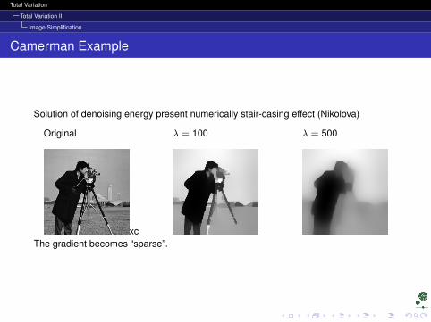
Camerman Example
Solution of denoising energy present numerically stair-casing effect (Nikolova)
Original
xc
λ = 100 λ = 500
The gradient becomes “sparse”.
Total Variation
Bibliography
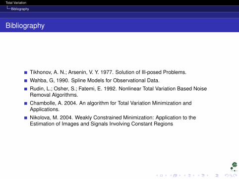
Bibliography
Tikhonov, A. N.; Arsenin, V. Y. 1977. Solution of Ill-posed Problems.
Wahba, G, 1990. Spline Models for Observational Data.
Rudin, L.; Osher, S.; Fatemi, E. 1992. Nonlinear Total Variation Based NoiseRemoval Algorithms.
Chambolle, A. 2004. An algorithm for Total Variation Minimization andApplications.
Nikolova, M. 2004. Weakly Constrained Minimization: Application to theEstimation of Images and Signals Involving Constant Regions
Total Variation
The End
The End