Technical Report Documentation Page

1. Report No. FHWA/TX-10/0-6210-1

2. Government Accession No.

3. Recipient’s Catalog No.

4. Title and Subtitle Tour-Based Model Development for TxDOT: Implementation Steps for the Tour-based Model Design Option and the Data Needs

5. Report Date October 2009

6. Performing Organization Code

7. Author(s) Nazneen Ferdous, Ipek N. Sener, Chandra R. Bhat, Phillip Reeder

8. Performing Organization Report No. 0-6210-1

9. Performing Organization Name and Address 10. Work Unit No. (TRAIS)

Center for Transportation Research The University of Texas at Austin 3208 Red River, Suite 200 Austin, TX 78705-2650

Texas Transportation Institute Texas A&M University 3135 TAMU College Station, TX 77843

11. Contract or Grant No. 0-6210

12. Sponsoring Agency Name and Address Texas Department of Transportation Research and Technology Implementation Office P.O. Box 5080 Austin, TX 78763-5080

13. Type of Report and Period Covered Technical Report 9/1/08-8/31/09

14. Sponsoring Agency Code

15. Supplementary Notes Project performed in cooperation with the Texas Department of Transportation and the Federal Highway Administration.

16. Abstract Travel demand modeling, in recent years, has seen a paradigm shift with an emphasis on analyzing travel at the individual level rather than using direct statistical projections of aggregate travel demand as in the trip-based approach. Specifically, several metropolitan planning organizations (MPO) in the U.S are developing and implementing advanced travel demand models that are based on a behaviorally more realistic representation of demand for travel. In addition, a number of planning agencies are considering the transition toward advanced travel demand modeling, TxDOT being one of them. Toward this end, this report provides the details of implementing a tour-based travel demand model system. Specifically, the implementation steps are provided for a tour-based model system (with no recognition of the interactions among tours). This includes discussion on data assembly and data preparation, model estimation and calibration (validation), trip assignment output validation, and software recommendations and budgetary considerations. 17. Key Words Implementation of a tour-based model system, Data needs for tour-based modeling

18. Distribution Statement No restrictions. This document is available to the public through the National Technical Information Service, Springfield, Virginia 22161; www.ntis.gov.

19. Security Classif. (of report) Unclassified

20. Security Classif. (of this page) Unclassified

21. No. of pages 38

22. Price

Form DOT F 1700.7 (8-72) Reproduction of completed page authorized

Tour-Based Model Development for TxDOT: Implementation Steps for the Tour-based Model Design Option and the Data Needs The University of Texas at Austin, CTR Nazneen Ferdous Ipek N. Sener Chandra R. Bhat Texas A&M University, TTI Phillip Reeder CTR Technical Report: 0-6210-1 Report Date: October 2009 Project: 0-6210 Project Title: Adding Tour-Based Modeling to TxDOT's Travel Modeling Framework Sponsoring Agency: Texas Department of Transportation Performing Agency: Center for Transportation Research at The University of Texas at Austin and

Texas Transportation Institute, Texas A&M University Project performed in cooperation with the Texas Department of Transportation and the Federal Highway Administration.

iv

Center for Transportation Research The University of Texas at Austin 3208 Red River Austin, TX 78705 www.utexas.edu/research/ctr Copyright (c) 2009 Center for Transportation Research The University of Texas at Austin All rights reserved Printed in the United States of America

v

Disclaimers Author's Disclaimer: The contents of this report reflect the views of the authors, who

are responsible for the facts and the accuracy of the data presented herein. The contents do not necessarily reflect the official view or policies of the Federal Highway Administration or the Texas Department of Transportation (TxDOT). This report does not constitute a standard, specification, or regulation.

Patent Disclaimer: There was no invention or discovery conceived or first actually reduced to practice in the course of or under this contract, including any art, method, process, machine manufacture, design or composition of matter, or any new useful improvement thereof, or any variety of plant, which is or may be patentable under the patent laws of the United States of America or any foreign country.

Notice: The United States Government and the State of Texas do not endorse products or manufacturers. If trade or manufacturers' names appear herein, it is solely because they are considered essential to the object of this report.

Engineering Disclaimer NOT INTENDED FOR CONSTRUCTION, BIDDING, OR PERMIT PURPOSES.

Project Engineer: Chandra R. Bhat

Professional Engineer License State and Number: Texas No. 88971 P. E. Designation: Research Supervisor

vi

Acknowledgments The authors would like to thank Janie Temple and Greg Lancaster for their input and

guidance during the course of this research project.

vii

Table of Contents

Chapter 1. Overview ..................................................................................................................... 1

Chapter 2. Data Development ...................................................................................................... 3 2.1 Household Activity and/or Travel Survey Data ....................................................................3

2.1.1 Data Screening ............................................................................................................... 3 2.1.2 Forming Tours from Travel Diary Data ......................................................................... 3

2.2 Land-use Data ........................................................................................................................4 2.2.1 Traffic Analysis Zone (TAZ) ......................................................................................... 4 2.2.2 Demographic Data ......................................................................................................... 4

2.3 Transportation Network and System Performance Data .......................................................5

Chapter 3. Model Development ................................................................................................... 7 3.1 Population Synthesizer and the Long-Term Choice Models .................................................7

3.1.1 Household Population Synthesizer ................................................................................ 9 3.1.2 Workplace Location Choice Model ............................................................................. 10 3.1.3 Household Vehicle Ownership Model ......................................................................... 10

3.2 Activity-Travel Generation Module ....................................................................................11 3.2.1 Pattern-Level Models ................................................................................................... 11 3.2.2 Tour Type Models ........................................................................................................ 12

3.3 Scheduling Module ..............................................................................................................12 3.3.1 Location Choice Models .............................................................................................. 13 3.3.2 Mode Choice Models ................................................................................................... 14

Chapter 4. Validation ................................................................................................................. 17 4.1 Highway Assignment ...........................................................................................................17 4.2 Transit Assignment ..............................................................................................................17

Chapter 5. Application Software and Other Implementation Issues ..................................... 19 5.1 Software System ..................................................................................................................19 5.2 Budget and Timeline for Development ...............................................................................21

Chapter 6. Summary .................................................................................................................. 23

References .................................................................................................................................... 25

viii

ix

List of Figures Figure 3.1: Structure of the Tour-based Design Model System ..................................................... 8

Figure 3.2: Possible Nesting Structure for Tour Mode Choice Models ....................................... 15

Figure 5.1: Proposed Decomposition Structure of the Software Architecture ............................. 20

x

xi

List of Tables Table 3.1: The Tour-Trip Mode Combinations to be Modeled in the Design Option #1 ............. 14

Table 5.1: Tentative Cost Estimates for the Development of tour-based design model for a Pilot Case Study ............................................................................................................. 22

xii

1

Chapter 1. Overview

Travel demand modeling, in recent years, has seen a paradigm shift with an emphasis on analyzing travel at the individual level rather than using direct statistical projections of aggregate travel demand as in the trip-based approach. Specifically, several metropolitan planning organizations (MPO) in the U.S. are developing and implementing advanced travel demand models that are based on a behaviorally more realistic representation of demand for travel. In addition, a number of planning agencies are considering the transition toward advanced travel demand modeling, TxDOT being one of them. Toward this end, this report provides the details of implementing a tour-based travel demand model system. The implementation steps includes discussion on data assembly and data preparation (Chapter 2), model estimation and calibration validation (Chapter 3), trip assignment output validation (Chapter 4), and software recommendations and budgetary considerations (Chapter 5).

2

3

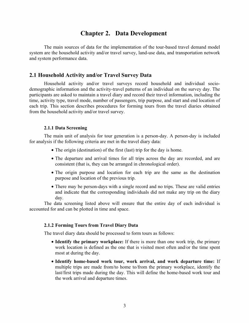
Chapter 2. Data Development

The main sources of data for the implementation of the tour-based travel demand model system are the household activity and/or travel survey, land-use data, and transportation network and system performance data.

2.1 Household Activity and/or Travel Survey Data Household activity and/or travel surveys record household and individual socio-

demographic information and the activity-travel patterns of an individual on the survey day. The participants are asked to maintain a travel diary and record their travel information, including the time, activity type, travel mode, number of passengers, trip purpose, and start and end location of each trip. This section describes procedures for forming tours from the travel diaries obtained from the household activity and/or travel survey.

2.1.1 Data Screening The main unit of analysis for tour generation is a person-day. A person-day is included

for analysis if the following criteria are met in the travel diary data:

• The origin (destination) of the first (last) trip for the day is home.

• The departure and arrival times for all trips across the day are recorded, and are consistent (that is, they can be arranged in chronological order).

• The origin purpose and location for each trip are the same as the destination purpose and location of the previous trip.

• There may be person-days with a single record and no trips. These are valid entries and indicate that the corresponding individuals did not make any trip on the diary day.

The data screening listed above will ensure that the entire day of each individual is accounted for and can be plotted in time and space.

2.1.2 Forming Tours from Travel Diary Data The travel diary data should be processed to form tours as follows:

• Identify the primary workplace: If there is more than one work trip, the primary work location is defined as the one that is visited most often and/or the time spent most at during the day.

• Identify home-based work tour, work arrival, and work departure time: If multiple trips are made from/to home to/from the primary workplace, identify the last/first trips made during the day. This will define the home-based work tour and the work arrival and departure times.

4

• Identify work-based subtour: Any trips made between the first arrival at the work location and last departure from the work location will be classified as work-based subtours.

• Identify and define home-based non-work tours: Classify any remaining trips into before and/or after the work tour. A new tour begins when the origin is home and a tour ends when the destination is home (then the tour is home-based). In determining the tour purpose, the following order of the priority should be maintained: school, other (personal business, meals, etc.), shopping, social and recreational, and drop off/pickup. In a tour, the trip purpose with the highest priority should determine the tour purpose.

• Identify the primary and the secondary destinations: The tour purpose will determine the location of the primary destination. If there is more than one destination with the same purpose, then, the one with the longest duration of stay is the primary destination. The rest of the trip destinations in a tour will be designated as secondary destinations.

• Identify tour and trip modes: Accumulate the travel time spent in each type of mode during each tour. The available modes are drive alone (DA), shared ride (SR), transit, bike, and walk. The trip modes in a tour should fall into one of these categories. The tour mode is determined as the mode in which the longest time is spent.

The final tour file should have one record for each tour with detailed tour-level and trip-level information. The relevant household and individual socio-demographic information, land-use data and the level of service data should subsequently be appended to the tour file appropriately. In addition, several checks will need to be undertaken to ensure the consistency of the sample data.

2.2 Land-use Data This section describes the steps for preparing the land-use data for the tour-based model.

2.2.1 Traffic Analysis Zone (TAZ) To make the transition from the trip-based to the tour-based model easier, the research

team recommends that the TAZs as defined for each MPO (and as included in the Texas Package) be maintained in the tour-based modeling approach.

2.2.2 Demographic Data The Texas MPOs, in conjunction with the Transportation Planning and Programming

(TP&P) Division of TxDOT, develops the following socioeconomic data for each TAZ in the base year and the forecast year:

• Total population,

• Number of households,

5

• Median household income,

• Total employment by different categories (basic, retail, service, and education), and

• Special generator (regional mall, airport, hospital, college, etc.). Since the data is already generated at the TAZ level for the Texas Package, no additional

data processing is required for the development of the tour-based model system.

2.3 Transportation Network and System Performance Data The MPOs in Texas collect and maintain a transportation network database that lists the

physical characteristics of the network, including the number of lanes, posted speed limit, direction (one-way or two-way facility), median access type (divided, undivided or continuous left turn), and functional classification. For each link, the TxDOT-TP&P Division develops additional information including link length, area type, link capacity, and speed. The TransCAD software is used to calculate link length and the travel time matrix between each origin-destination (O-D) pair. The travel time matrix represents the minimum network travel time path for each O-D pair. All the network data mentioned above can be directly incorporated, without any additional data processing, for the development of the tour-based model.

Every year, TxDOT-TPP collects 24-hour saturation counts on a number of urban roadways and state highways. This count data is currently used to validate the travel model in the Texas Package. The count data used for the trip-based model validation can also be used, without any additional processing, for the validation of the tour-based model system.

The Texas urban area comprehensive travel surveys include an on-board public transit survey component. The survey collects information on trip origins and destinations, mode of travel to/from transit stop, trip purpose, transit routes taken during trip, ridership frequency, transit fare paid and method of payment, and the traveler’s household characteristics (such as household vehicle availability, household size and household income). This survey data can be used, with no/very little additional processing, for the calibration and validation of the tour-based mode choice models.

6

7

Chapter 3. Model Development

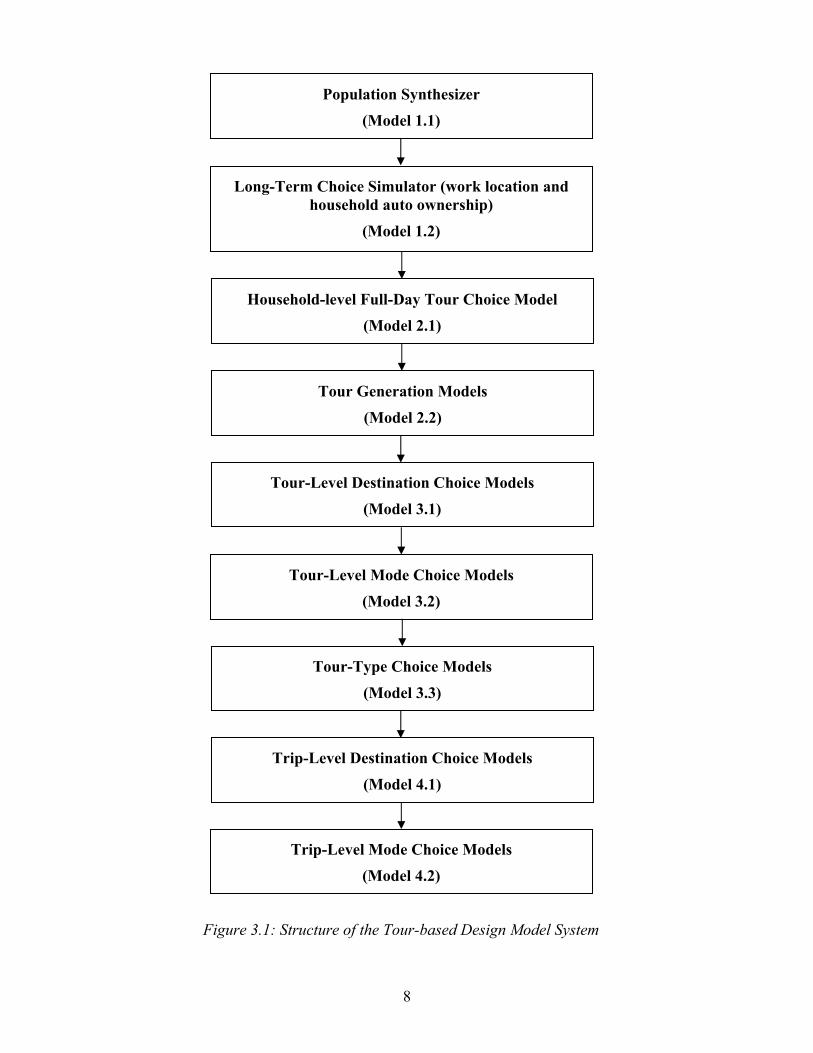
The sequence in which travel decisions are to be modeled in the tour-based design model is presented in Figure 3.1.. Based on their functionality (rather than the sequence of application), the models in the Figure 3.1 can be grouped into three categories:

• Models 1.1 and 1.2 generate the synthetic population and the long-term choices.

• Models 2.1, 2.2, and 3.3 together constitute the activity-travel generation module, which provide as outputs a list of all the activities, tours, and trips generated for the day.

• Models 3.1, 3.2, 4.1 and 4.2 schedule the generated activities, tours, and trips; these models can be labeled as the scheduling module. Models in the scheduling module determine the where (destination) and how (mode) of the generated activities and travel.

3.1 Population Synthesizer and the Long-Term Choice Models The population synthesizer and the long-term choice module of tour-based design model

include three models:

1) Household population synthesizer,

2) Work location choice model, and

3) Household vehicle ownership model.

8

Figure 3.1: Structure of the Tour-based Design Model System

Population Synthesizer

(Model 1.1)

Long-Term Choice Simulator (work location and household auto ownership)

(Model 1.2)

Household-level Full-Day Tour Choice Model

(Model 2.1)

Tour-Level Destination Choice Models

(Model 3.1)

Tour-Level Mode Choice Models

(Model 3.2)

Tour Generation Models

(Model 2.2)

Trip-Level Mode Choice Models

(Model 4.2)

Trip-Level Destination Choice Models

(Model 4.1)

Tour-Type Choice Models

(Model 3.3)

9

3.1.1 Household Population Synthesizer The tour-based design model system starts with a population synthesizer that is designed

to create a list of synthetic households (and individuals) in each TAZ with information on the control variables. The control variables used here include zonal-level values for mean household size, number and age distribution of children, number of workers, and household income. These basic inputs for the control variables can be obtained from a land-use model, or be defined directly by the user from data sources available with the Texas State Data Center.

Next, the control variables are categorized as follows to classify sampling “cells”:

• Household (HH) size - one person HH, two persons HH, and three + persons HH.

• Number and age group of children - HH with no children, HH with one child, and HH with two or more children. Each HH is then further classified into one of the three groups depending on the age of the children: HH own children age less than 4 years, HH own children aged between 4 and 10 years, and HH own children between 10 and 15 years.

• Number of workers - zero workers, one worker, two workers, and three + workers.

• HH income - income < 20k, 20k ≤ income < 35k, 35k ≤ income < 50k, 50k ≤ income < 75k, and income ≥ 75k.

The categories for household size, number and age group of children, and number of workers were chosen because they distinguish important family lifecycle groups. The breakdown for income was chosen because it is compatible with both the household survey undertaken by TxDOT and the Census tables available in the Census Transportation Planning Package (CTPP) 2000. The combinations of the categories across the four control variables result in 195 (39 x 5) different sampling cells in total.1

The population synthesis procedure is implemented for each TAZ, using the seed distribution of households observed in the Public Use Microdata Sample (PUMS). Iterative proportional fitting (IPF) is used to estimate the number of households within each cell in each TAZ. At the end of this procedure, for each cell in each TAZ, the synthesizer will generate a list of households with household size, number, and age distribution of children, number of workers, and household income group. Once the number of households for each of the 195 cells is estimated for a given TAZ, PUMS data is used to randomly sample the correct number of households within each cell. Since the PUMS constitutes a 5% sample, each PUMS household will appear in the full sample twenty times for each draw. The resulting sample file will contain the PUMS household ID number, the TAZ number, and the sampling cell number. Using this information, the relevant household and person level data (available in the PUMS records) can be appended to the sample file, which can subsequently be used in the travel demand models. The reader is referred to Guo and Bhat (2007) for technical details of the synthetic population generation procedure that may be employed.

1 Not each of the 84 (3*7*4) HH size-number and age group of children-number of workers combination is feasible. For example, HH with 1 person will not have any children and can have at most 1 worker. This reduces the number of possible combinations of these three control variables to 39.

10

3.1.2 Workplace Location Choice Model The work location model is the first component of the model system for application, and

hence only variables in the PUMS-based synthetic population can be used to estimate work location choice model. These could include residence location (CBD, urban, suburban, etc.), household and individual characteristics (household income, number of workers, presence and age of children, number of licensed drivers, etc.), and origin and destination zone characteristics (population, household and employment densities, retail space, same zone indicator, etc.). The model will be estimated using a multinomial logit structure where the number of choice alternatives can potentially be equal to the number of TAZs. However, depending on the size of the study area, the estimation process can be made significantly faster and less cumbersome if only a subset of TAZs is considered as being in the choice set for each worker. This can be achieved by classifying the TAZs into a number of ordered categories and sampling from each category according to their importance. A number of criteria can be used to define the importance of a particular category. For example, zonal employment can be used to classify the TAZs into a number of categories.

For model estimation (and validation), data collected by TxDOT as part of the household survey will be used. The estimation data should include only the worker residents (full time or part time) of the study area. To ensure that the origin TAZs are within the proper range, the data sample should be checked for consistency, and, in turn, data with TAZ numbers outside the range, missing TAZ numbers, or work tours that do not originate at home need to be removed.2 The model is applied to predict the work location for each worker in the sample, which is then used as the primary destination for all work-related tours made by the corresponding individual.

3.1.3 Household Vehicle Ownership Model The number of vehicles available to a household is defined as the number of cars, vans,

and light trucks owned/leased by the household members. The vehicle ownership model is a multinomial logit model with the following potential choice alternatives:

• Household with no car,

• Household with one car,

• Household with two cars,

• Household with three cars, and

• Household with four or more cars. A number of household socio-demographic, residential location and accessibility

variables need to be tested for inclusion in the model specification. The household socio-demographic variables may include number of adults, number of workers, number of children, number of licensed drivers, and household income. Residential location variables may include residential density and type of area (CBD, urban, suburban, etc.). Accessibility variables may include auto travel time and cost, transit travel time and fare, parking availability, and cost of parking. The final model specification will be based on a systematic process of removing statistically insignificant variables, and combining variables when their effects were not 2 Since only home-based and work-based tours are modeled, tours that do not originate at either of these two locations are excluded from the model estimation data set.

11

significantly different. The specification process should also be guided by prior research, intuitiveness/parsimony considerations, and TxDOT suggestions.

The vehicle ownership model may be applied for each synthetic household to calculate the probability of having a certain number of vehicles. The model can be estimated using the available survey data. Depending on the sample size, a subset of the survey data that has not been used in model estimation can be used for validation. In addition, the model prediction can be compared against the Department of Motor Vehicle (DMV) and the Census data. The model prediction can also be validated against aggregate survey data (total number of households with no car, total number of households with one car, etc.) as well as data stratified by segments (for example, HH with no workers, single worker HH, and multiple workers HH).

3.2 Activity-Travel Generation Module The activity-travel generation module may be considered similar in function to the trip

generation step in a four-step trip-based model. This module provides a list of all the activities, tours, and stops generated by a household in a day. As stated before, the activity-travel generation module consists of three distinct model categories: 1) Daily tour choice model (Model 2.1 in Figure 3.1), 2) Tour generation models (Model 2.2 in Figure 3.1), and 3) Tour type models (Model 3.3 in Figure 3.1). Note that the former two models together can be referred as the pattern-level models, as discussed in the next section.

3.2.1 Pattern-Level Models As mentioned in the paragraph above, the pattern-level models consist of two model

types:

• Daily tour choice model (Model 2.1 in Figure 3.1), and

• Tour generation models (Model 2.2 in Figure 3.1). The daily tour choice model is a binary logit model, and predicts whether or not a

household makes tours for a particular activity purpose in a day. The tour generation models then determine the number of tours for each activity purpose made by the household. This may be undertaken within a multinomial logit framework. Depending on the available data, the choice alternatives for each purpose may include one, two, three, and four + tours made by a household.

The tours are divided into six purposes and are generated in the following order:

• Home-based school tours,

• Home-based work tours,

• Home-based other tours (includes personal business, meals),

• Home-based shopping,

• Home-based social/recreational tours, and

• Home-based drop off/pickup tours. All tours are assumed to fit into one of these categories. An advantage of adopting this

hierarchy of tour purposes is that all tours generated by a household are interrelated. This is achieved by using tour frequencies of a particular purpose higher up in the model system as

12

explanatory variables in the subsequent tour type models. For illustration, consider a nuclear family household with two working adults and a school-going child. If, due to sickness or some other reason, the child does not go to school and stays at home, then one of the parents is likely to stay at home and take care of the child. The impact on the activity participation pattern of adult household members due to a change in the home-based school tour pattern of young household members can then be incorporated in the model system.

Travel survey data with detailed information on out-of-home activities and travel can be used for model estimation and validation of the daily tour choice and tour generation models. The entire data set may be used to estimate a single model (for a particular purpose), or the data set may be segmented to estimate multiple models. For example, for the home-based work tours, the data set can be segmented into single-individual households, two-individual households, and multiple-individual households to differentiate the distinct work tour frequencies and patterns of households of different sizes. The decision whether to estimate a single model or multiple models will depend on the observed distribution of the tour frequencies.

3.2.2 Tour Type Models Tour type models (Model 3.3 in Figure 3.1) generate the number of stops on a tour for all

tour purposes and whether a work tour has a subtour associated with it or not. To increase computational efficiency, the maximum number of stops associated with a tour is limited to five (one stop to the primary destination and four intermediate stops to the secondary destinations).3 The subtours have work location as origin and destination, and can have only one stop.

The tour type models may be formulated with a multinomial logit structure using travel survey data. The models will be applied to each type of tour after the estimation of tour-level mode choice models (Model 3.2 in Figure 3.1)4. This will provide the opportunity to use tour mode as an explanatory variable in the tour type models. In addition, because of ease of travel and flexibility of using personal vehicles, it is likely that tours made by the auto mode have different travel patterns from, for example, tours made by transit. Based on data analysis, tours made by auto and non-auto modes may be modeled separately to yield behaviorally more realistic predictions. Further, the number of stops in a tour and subtour will be generated in the following order: school tours, work-based subtour, other tours, shopping tours, social/recreational tours, and drop off/pickup tours. Additional variables that should be considered for inclusion in the models include household size, number of workers, income, number of tours for purposes higher in the hierarchy, and residential location type.

3.3 Scheduling Module The tours and the stops generated by a household in a day (as discussed in Section 3.2)

are scheduled using the models discussed in Sections 3.3.1 and 3.3.2.

3 For ease of presentation, the same maximum number of stops is used for all activity purposes here. However, the maximum number of stops associated with a tour can be different for different activity purposes. This can be easily incorporated once the final survey data are made available. 4 The reader will note that the tour-level mode choice models are part of the Scheduling Module, which is discussed in the next section (Section 3.3).

13

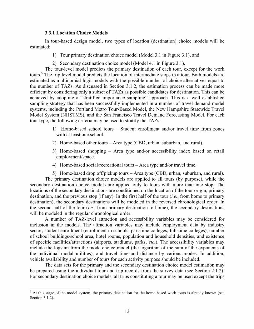
3.3.1 Location Choice Models In tour-based design model, two types of location (destination) choice models will be

estimated:

1) Tour primary destination choice model (Model 3.1 in Figure 3.1), and

2) Secondary destination choice model (Model 4.1 in Figure 3.1). The tour-level model predicts the primary destination of each tour, except for the work

tours.5 The trip level model predicts the location of intermediate stops in a tour. Both models are estimated as multinomial logit models with the possible number of choice alternatives equal to the number of TAZs. As discussed in Section 3.1.2, the estimation process can be made more efficient by considering only a subset of TAZs as possible candidates for destination. This can be achieved by adopting a “stratified importance sampling” approach. This is a well established sampling strategy that has been successfully implemented in a number of travel demand model systems, including the Portland Metro Tour-Based Model, the New Hampshire Statewide Travel Model System (NHSTMS), and the San Francisco Travel Demand Forecasting Model. For each tour type, the following criteria may be used to stratify the TAZs:

1) Home-based school tours – Student enrollment and/or travel time from zones with at least one school.

2) Home-based other tours – Area type (CBD, urban, suburban, and rural).

3) Home-based shopping – Area type and/or accessibility index based on retail employment/space.

4) Home-based social/recreational tours – Area type and/or travel time.

5) Home-based drop off/pickup tours – Area type (CBD, urban, suburban, and rural). The primary destination choice models are applied to all tours (by purpose), while the

secondary destination choice models are applied only to tours with more than one stop. The locations of the secondary destinations are conditioned on the location of the tour origin, primary destination, and the previous stop (if any). In the first half of the tour (i.e., from home to primary destination), the secondary destinations will be modeled in the reversed chronological order. In the second half of the tour (i.e., from primary destination to home), the secondary destinations will be modeled in the regular chronological order.

A number of TAZ-level attraction and accessibility variables may be considered for inclusion in the models. The attraction variables may include employment data by industry sector, student enrollment (enrollment in schools, part-time colleges, full-time colleges), number of school buildings/school area, hotel rooms, population and household densities, and existence of specific facilities/attractions (airports, stadiums, parks, etc.). The accessibility variables may include the logsum from the mode choice model (the logarithm of the sum of the exponents of the individual modal utilities), and travel time and distance by various modes. In addition, vehicle availability and number of tours for each activity purpose should be included.

The data sets for the primary and the secondary destination choice model estimation may be prepared using the individual tour and trip records from the survey data (see Section 2.1.2). For secondary destination choice models, all trips constituting a tour may be used except the trips

5 At this stage of the model system, the primary destination for the home-based work tours is already known (see Section 3.1.2).

14

to the primary destination, home, and work locations. The tour purpose—instead of trip purpose—will be used to group trips together for estimation. For calibration and validation, the model prediction can be compared against such observed data as (1) the frequency of the tours and trips by origin and destination area types (for example CBD, urban, suburban, and rural), (2) the percentage by origin (destination) area type within each of the destination (origin) area types, and (3) travel time.

3.3.2 Mode Choice Models Mode choice models perform a similar task as the modal split step in the four-step travel

demand models. The design option includes two types of mode choice models:

1) Tour-level mode choice models (Model 3.2 in Figure 2.1), and

2) Trip-level mode choice models (Model 4.2 in Figure 2.1) The tour mode choice models determine the primary mode for the tour while the trip

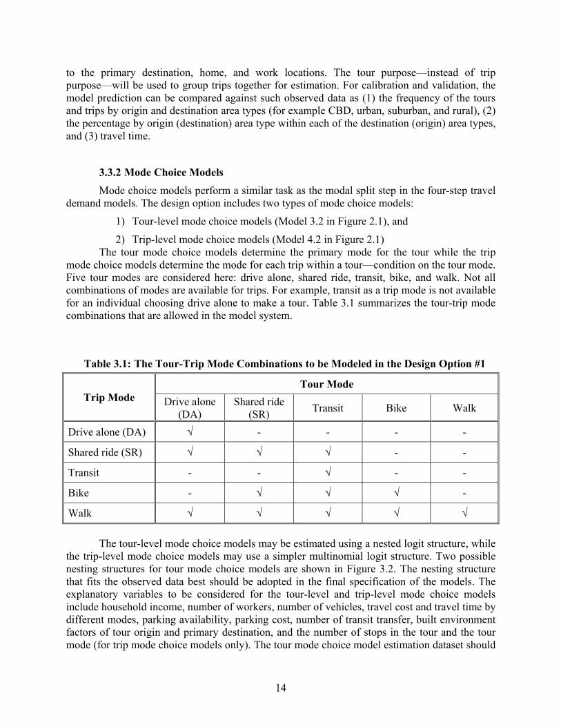
mode choice models determine the mode for each trip within a tour—condition on the tour mode. Five tour modes are considered here: drive alone, shared ride, transit, bike, and walk. Not all combinations of modes are available for trips. For example, transit as a trip mode is not available for an individual choosing drive alone to make a tour. Table 3.1 summarizes the tour-trip mode combinations that are allowed in the model system.

Table 3.1: The Tour-Trip Mode Combinations to be Modeled in the Design Option #1

Trip Mode Tour Mode

Drive alone (DA)

Shared ride (SR) Transit Bike Walk

Drive alone (DA) √ - - - -

Shared ride (SR) √ √ √ - -

Transit - - √ - -

Bike - √ √ √ -

Walk √ √ √ √ √

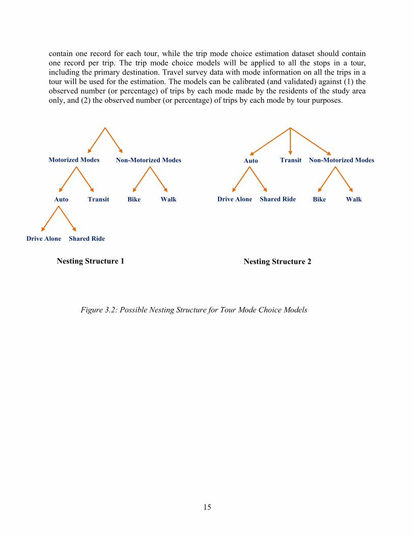
The tour-level mode choice models may be estimated using a nested logit structure, while the trip-level mode choice models may use a simpler multinomial logit structure. Two possible nesting structures for tour mode choice models are shown in Figure 3.2. The nesting structure that fits the observed data best should be adopted in the final specification of the models. The explanatory variables to be considered for the tour-level and trip-level mode choice models include household income, number of workers, number of vehicles, travel cost and travel time by different modes, parking availability, parking cost, number of transit transfer, built environment factors of tour origin and primary destination, and the number of stops in the tour and the tour mode (for trip mode choice models only). The tour mode choice model estimation dataset should

15

contain one record for each tour, while the trip mode choice estimation dataset should contain one record per trip. The trip mode choice models will be applied to all the stops in a tour, including the primary destination. Travel survey data with mode information on all the trips in a tour will be used for the estimation. The models can be calibrated (and validated) against (1) the observed number (or percentage) of trips by each mode made by the residents of the study area only, and (2) the observed number (or percentage) of trips by each mode by tour purposes.

Figure 3.2: Possible Nesting Structure for Tour Mode Choice Models

Non-Motorized ModesMotorized Modes

Bike WalkTransit Auto

Drive Alone Shared Ride

Non-Motorized Modes

Bike Walk

Transit Auto

Drive Alone Shared Ride

Nesting Structure 1 Nesting Structure 2

16

17

Chapter 4. Validation

The validation of individual components of the activity-travel system has already been discussed in the previous section. In this section, only the validation of the results at the end of the traffic assignment step is discussed. The reader will note that, once the activity-travel pattern of each individual is obtained from the implementation of the models in Figure 3.1, these patterns can be translated into trip origin-destination matrices by time of day for internal-internal trips. These matrices will need to be updated by adding trip matrices corresponding to external trips and freight-related trips, which have to be obtained externally using procedures already in place by TxDOT. The final origin-destination matrices by time of day may be assigned to obtain link volumes and speeds based on the current static assignment procedure employed by TxDOT.

4.1 Highway Assignment Highway assignments will be primarily validated against observed traffic volumes. The

traffic count data is collected as 24-hour counts. Therefore, the highway assignment results will be compared against daily traffic flows. The individual link flows will be aggregated to compare against volumes by corridors and volumes by facility types. For volumes by corridor, a number of screenlines will be defined, and the observed traffic volume and the predicted traffic volume will be compared by screenline. For volume by facility types, the predicted link flows will be aggregated by facility types (freeway, arterial, collector, local, etc.), and compared against observed volumes. In addition, predicted network speeds at strategic locations and travel times will be compared against observed data to ensure that these are accurately represented in the models. All of these validation steps are similar to those already being pursued in the context of the trip-based model predictions.

4.2 Transit Assignment The observed transit data is collected by transit on-board surveys. Although the survey

data contains detailed information on time period, the proposed model will only be able to predict daily transit boardings. For validation, observed daily transit boardings will be compared against the predicted transit boardings at an aggregate level as well as by individual route (or similar routes grouped together).

18

19

Chapter 5. Application Software and Other Implementation Issues

5.1 Software System TxDOT maintains a list of recommended development languages for application software

development; these recommended development languages are:

• Visual Basic

• C#

• C++

• J#

• Perl A permissible alternative development language is Java; however, the use of Java would

require that an exception request be submitted to TxDOT’s Technology Services Division (TSD). For the proposed tour-based modeling system, it recommended that the core model system be developed using Visual C++, a flexible language that also provides the benefit of relatively easily generating visual interfaces. This should be helpful, among other things, in building a user-friendly interface with the Texas Package and TransCAD.

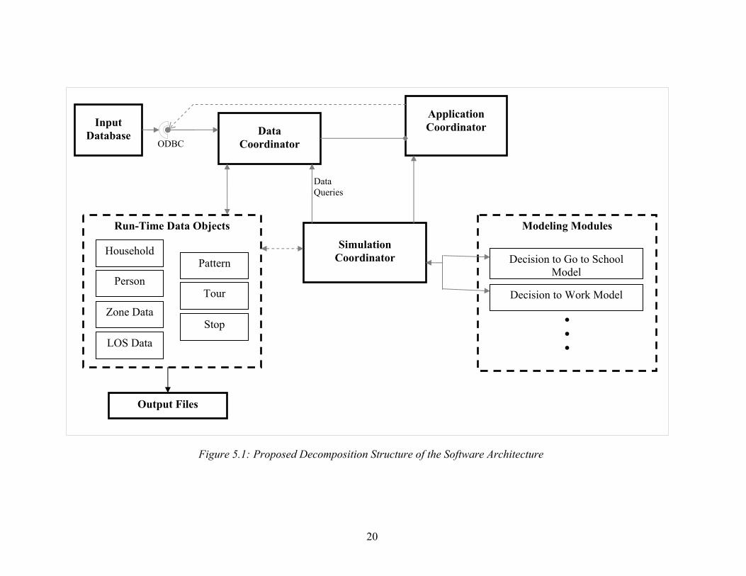
The application of the tour-based model will require a significant amount of computing resources, as well as careful management of a large number of computer files. Based on past experience, the research team recommends the use of computers with Windows 2000 Professional or XP Operating System and a minimum of a 1 GHZ Processor, 4 GB RAM, and 210 GB Hard Drive. For the software architecture, we propose a streamlined configuration as shown in Figure 5.1. The major components of the model system are the input database, data coordinator, run-time data objects, modeling modules, simulation coordinator, application coordinator, and output files. As mentioned earlier, the simulation of activity-travel patterns is a data intensive exercise. Therefore, we propose the input data to be stored in a relational database management system (DBMS). The reason for choosing a DBMS to store data is to leverage on the last 30 to 40 years of research advances in storage, organization, query, and management of large volumes of data. Next, the data coordinator creates instances of household, person, zone-to-zone, and level-of-service (LOS) entities from the input database. The modeling modules simulate the activity-travel patterns generated by households while the simulation coordinator generates the patterns, tours, and the stops. The run-time data objects act as a cache for the simulation coordinator that frequently accesses data. The application driver starts and runs the application. Finally, the outputs are written using the output files module. The format of the output files can be selected through the Graphical User Interface (GUI). To maintain ease and flexibility, we recommend the outputs be stored in flat-files (plain tabbed formatted files).

As shown in Figure 5.1, we recommend that the model system interact with a relational DBMS through an open database connectivity (ODBC). One of the reasons for this is that ODBC provides a product-independent interface between client applications (Design Option #1 model system, in this case) and database servers, allowing applications to be portable between database servers from different manufacturers. We also recommend employment of several performance enhancement strategies, including multithreading and data caching.

20

Figure 5.1: Proposed Decomposition Structure of the Software Architecture

ODBC

Run-Time Data Objects

Household

Person

Zone Data

LOS Data

Pattern

Tour

Stop

Output Files

Simulation Coordinator

Modeling Modules . . .

Decision to Go to School Model

Decision to Work Model

Input Database Data

Coordinator

Application Coordinator

Data Queries

21

5.2 Budget and Timeline for Development An informal investigation of funding needs for the development of a full-fledged activity-

based model revealed that, depending on the study area and complexity of the model, the budget resources required for the development of a tour-based model could range from $1 million to $1.4 million (Transportation Research Board of the National Academies (2007) Special Report 288). But, in the case of TP&P, there can be considerable economies of scale since (1) the proposed tour-based model system has a relatively simple structure (i.e., no interaction across tours), (2) the survey data used for the development of the trip-based model can be used with little or no additional processing for the development of the tour-based model, and (3) the system can be applied to multiple urban areas under TP&P’s modeling jurisdiction with relatively little overhead to populate the model with local data and parameters.

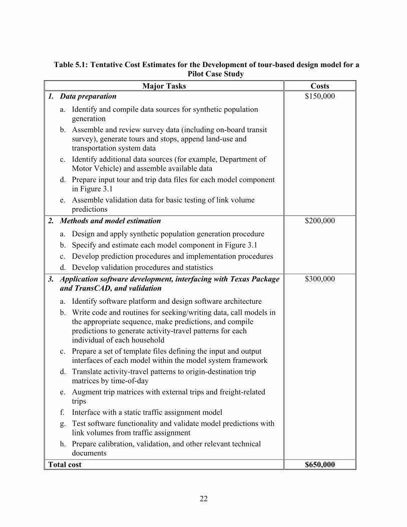
The team recommends that the entire enterprise of developing a tour-based model be focused on a single case study region to begin with, though the architecture for the model should be developed to be portable and transferable to any metropolitan region. The case study region should represent a “middle of the road” MPO among those whose travel modeling TP&P handles. We recommend that the study region also be chosen based on a metropolitan region that may see relatively substantial land-use and transportation network changes in the near-term, along with changes in demographic characteristics of the resident population. A desire by the MPO to be part of the development of a tour-based modeling framework for its metropolitan region would also be important, as would good GIS experience among the MPO staff and readily available land-use/transportation network files for the MPO region. For such a pilot case study, the estimated budget would be $650,000 (without considering overhead). Note, however, that this budget does not include extensive validation testing of individual components of the model system and/or validation using before/after or back-casting exercises. Rather, it includes the kind of basic validation that is currently undertaken with trip-based models. Table 5.1 provides a listing of the major tasks for the pilot development within each of three categories: (1) Data preparation ($100,000 estimated budget), (2) Methods and model estimation ($200,000 estimated budget), and (3) Application software development, interfacing with Texas Package and TransCAD, and validation ($300,000 estimated budget). The development timeline would be 24 months. Note that these budgets are for the pilot case study, and should be viewed as best estimates at this point. Once developed for the pilot area, the application of the software to additional metropolitan areas should entail a smaller budget and a much faster turnaround time in terms of application.

22

Table 5.1: Tentative Cost Estimates for the Development of tour-based design model for a Pilot Case Study

Major Tasks Costs 1. Data preparation

a. Identify and compile data sources for synthetic population generation

b. Assemble and review survey data (including on-board transit survey), generate tours and stops, append land-use and transportation system data

c. Identify additional data sources (for example, Department of Motor Vehicle) and assemble available data

d. Prepare input tour and trip data files for each model component in Figure 3.1

e. Assemble validation data for basic testing of link volume predictions

$150,000

2. Methods and model estimation a. Design and apply synthetic population generation procedure b. Specify and estimate each model component in Figure 3.1 c. Develop prediction procedures and implementation procedures d. Develop validation procedures and statistics

$200,000

3. Application software development, interfacing with Texas Package and TransCAD, and validation a. Identify software platform and design software architecture b. Write code and routines for seeking/writing data, call models in

the appropriate sequence, make predictions, and compile predictions to generate activity-travel patterns for each individual of each household

c. Prepare a set of template files defining the input and output interfaces of each model within the model system framework

d. Translate activity-travel patterns to origin-destination trip matrices by time-of-day

e. Augment trip matrices with external trips and freight-related trips

f. Interface with a static traffic assignment model g. Test software functionality and validate model predictions with

link volumes from traffic assignment h. Prepare calibration, validation, and other relevant technical

documents

$300,000

Total cost $650,000

23

Chapter 6. Summary

The main sources of data required for the implementation of the tour-based model design are household activity and/or travel survey, land-use data, and transportation network and system performance data—the same data currently being used for the development and/or updating of the trip-based models. The land-use and the transportation network and system performance data require no/very little additional processing to be used in the development of the tour-based model. The household activity and/or travel survey data requires additional processing to form tours from trips recorded in the travel diary. The necessary steps for tour development are outlined in Section 2.1.

The models in the tour-based model design can be grouped into three categories:

1) Population synthesizer and the long-term choice models,

2) Activity-travel generation module, and

3) Scheduling module. The population synthesizer generates synthetic population and households that are

allocated to the TAZs. The long-term choice models include work location choice model and household vehicle ownership model. For each synthetic individual and household, the long-term choice models predict work location and the number of vehicles owned by a household, respectively. The outputs from the population synthesizer and the long-term choice models are used as inputs in the subsequent models.

The activity-travel generation module provides a list of all the activities, tours, and trips generated by a household in a day. The generated tours and trips are scheduled using the scheduling module. For each tour generation and scheduling module, the model development steps are provided, including analytical methods to model travel patterns, econometric framework, choice alternatives, possible explanatory variables, and calibration (and validation) criteria.

The core model system may be developed using software programs such as Visual C++, interfaced with TransCAD and the Texas Package.

24

25

References

Bhat, C.R., J.Y. Guo, S. Srinivasan, and A. Sivakumar (2004) Comprehensive Econometric Microsimulator for Daily Activity-Travel Patterns. Transportation Research Record, 1894, 57-66.

Bowman, J.L., and M.A. Bradley (2005-2006) Activity-Based Travel Forecasting Model for SACOG: Technical Memos Numbers 1-11. Available at http://jbowman.net (accessed on January 20, 2008).

Bowman, J.L., M.A. Bradley and J. Gibb (2006) The Sacramento activity-based travel demand model: estimation and validation results. Paper presented at the European Transport Conference, September 2006, Strasbourg, France.

Bowman, J.L. and M.A. Bradley (2008) Activity-Based Models: Approaches Used to Achieve Integration among Trips and Tours Throughout the Day. Presented at the 2008 European Transport Conference, Leeuwenhorst, The Netherlands, October 2008.

Bradley, M.A. and J.L. Bowman (2006) A Summary of Design Features of Activity-Based Microsimulation Models for U.S. MPOs. White paper presented at the TRB Conference on Innovations in Travel Demand Modeling, May 21-23, 2006, Austin, Texas, 2006.

Bradley, M.A., J.L. Bowman, and J. Castiglione (2008) Activity Model Work Plan and Activity Generation Model. Work plan report prepared for Puget Sound Regional Council.

Cambridge Systematics (1998) New Hampshire Statewide Travel Model System Model Documentation Report.

Cambridge Systematics (2002) San Francisco Travel Demand Forecasting Model Development: Executive Summary, and Model Development Documentation Reports. Available at http://www.sfcta.org/content/category/6/78/225/ (accessed on February 1, 2008).

Davidson, W., R. Donnelly, P. Vovsha, J. Freedman, S. Ruegg, J. Hicks, J. Castiglione, and R. Picado (2007) Synthesis of First Practices and Operational Research Approaches in Activity-based Travel Demand Modeling. Transportation Research Part A, 41(5), 464-488.

Eluru, N., A.R. Pinjari, J.Y. Guo, I.N. Sener, S. Srinivasan, R.B. Copperman, and C.R. Bhat (2008) Population Updating System Structures and Models Embedded in the Comprehensive Econometric Microsimulator for Urban Systems. Transportation Research Record, 2076, 171-182.

Ferdous, N., I.N. Sener, and C.R. Bhat (2009). Tour-Based Model Development: A Review of Current Tour-Based Travel Demand Models. Progress report for the Texas Department of Transportation (TxDOT), January 2009.

26

Ferdous, N., I.N. Sener, and C.R. Bhat (2009). Tour-Based Model Development: Model Design Recommendations for TxDOT and Data Needs. Progress report prepared for the Texas Department of Transportation (TxDOT), May 2009.

Guo, J.Y., and C.R. Bhat (2007). Population Synthesis for Microsimulating Travel Behavior. Transportation Research Record, 2014, 92-101.

MORPACE International, Inc. (2002). Bay Area Travel Survey Final Report, March 2002. ftp://ftp.abag.ca.gov/pub/mtc/planning/BATS/BATS2000/

Parsons Brinckerhoff / PB Consult New York Best Practice Model (BPM) For Regional Travel Demand Forecasting 2004.

PB Consult (2005) The MORPC Travel Demand Model: Validation and Final Report.

Pinjari, A., N. Eluru, R. Copperman, I.N. Sener, J.Y. Guo, S. Srinivasan, and C.R. Bhat (2006) Activity-Based Travel-Demand Analysis for Metropolitan Areas in Texas: CEMDAP Models, Framework, Software Architecture and Application Results. Report 0-4080-8, prepared for the Texas Department of Transportation, October 2006.

Sharma, S., R. Lyford, and T. Rossi (1998) The New Hampshire Statewide Travel Model System. Accessed at onlinepubs.trb.org/Onlinepubs/circulars/EC011/sharma.pdf, on March 20, 2009.

Transportation Research Board of the National Academies (2007) Special Report 288 Travel Forecasting Current Practice and Future Direction. Committee for Determination of the State of the Practice in Metropolitan Area Travel Forecasting.

University of Washington, Cambridge Systematics, and C.R. Bhat (2001). Land Use and Travel Demand Forecasting Models Recommendations for Integrated Land Use and Travel Models. Final Report. Prepared for Puget Sound Regional Council.