tourism and growth in european countries: an application

ECONOMICSRESEARCH CENTER

ISCTEUNIDE - ECRAV FORÇAS ARMADAS1649-126 LISBON-PORTUGALhttp://erc.unide.iscte.pt

Working Paper- ISCTE Lisbon University Institute

Tourism and Growth

Felipa de Mello-Sampayo

in European Countries:

Sofia de Sousa-Vale

Working Paper - 05/10

- Lisbon University Institute

An Application of Likelihood-Based Panel Cointegration

Tourism and Growth in European Countries: An Application ofLikelihood-Based Panel Cointegration

Felipa de Mello-Sampayo†and Sofia de Sousa-Vale

†

†ISCTE–IUL Institute University of Lisbon

Abstract

The tourism and economic growth relationship is investigated for a panel of Europeancountries over the period 1988–2010. The results reveal that the variables contain a panel unitroot and they cointegrate in a panel perspective. The findings show that tourism enhanceeconomic growth for some countries in the sample.

JEL Classification: F43; C33; L83

Keywords: Tourism; Economic growth; Rank tests; Panel unit root tests; Panel cointegration

Postal address: ISCTE-IUL, Department of Economics, Av. Forcas Armadas, 1649–026,Lisbon, Portugal.

Author’s email: [email protected]

1

1 Introduction

As globalization reaches the remotest economies in the world, international tourism has beensteadily increasing, as well as the importance of the tourism industry for the economy of manycountries. According to the World Travel & Tourism Council (WTTC)1, Tourism was a majorsource of economic growth to European countries, especially in small countries such as Malta,where it averaged 11% of Gross Domestic Product (GDP) in 2008 but also in larger countries suchas Spain where the tourism sector amounted to 6.1% in the same period. In addition, Tourismrepresents an important source of foreign exchange receipts, contributing to an amelioratedbalance of payments. Thus, tourism plays, nowadays, a key role in boosting the countries’economies. Tourism-generated proceeds have come to represent an increasing employment,external revenue source, household income and government income.

In the literature on growth, the export-led growth hypothesis (see McKinnon, 1964) postu-lates that international tourism contributes to growth in two ways. In the first place, enhancingefficiency through competition between the local sectors and foreign destinations (Bhagwati andSrinivasan, 1979, Krueger, 1980). Secondly, by facilitating the exploitation of economies of scalein local firms (Helpman and Krugman, 1985).

The growing importance of tourism on the national economies led to the emergence of theTourism Satellite Account2 (TSA) worldwide that provides a means of separating and examin-ing both tourism supply and tourism demand within the general framework of the System ofNational Accounts and, simultaneously, important contributions have been made to estimateempirically different forms and degrees of tourism on long-run economic growth (see Balaguerand Cantavella-Jorda, 2002, Eugenio-Martin, 2004, Oh, 2005, Gunduz and Hatemi-J., 2005, Leeand Chang, 2008, Katircioglu, 2009).

The branch of empirical research on the effects of tourism on economic growth that focuseson a single country and cointegrates gross domestic product (GDP) with the number of touristarrivals (or alternatively with the volume of tourism receipts) and real exchange rate3 has foundthat tourism has generally a positive impact on economic growth. Balaguer and Cantavella-Jorda (2002) tested the tourism-led growth hypothesis for Spain through cointegration andcausality tests relating real GDP, international tourism earnings and the real effective exchangerate, confirming the existence of a stable relationship between economic growth and tourism.They also found causality from tourism activity to economic growth. Gunduz and Hatemi-J. (2005) tested the tourism-led growth hypothesis for Turkey applying a causality test basedon leverage bootstrap simulations between the number of tourist arrivals, real gross domesticproduct and real exchange rates. They support empirically the tourism-led growth hypothesis.Katircioglu (2009) used cointegration and Granger causality tests to analyze the existence of along-run equilibrium relationship between tourism, trade and real income growth and concludethat real income growth stimulates growth in international trade but also stimulates the inter-national tourist arrivals into Cyprus. Further, it was found that the international trade’s growthstimulates tourist arrivals into the island.

The empirical research focussing on a panel of countries also provides evidence of a long-runrelationship between tourism development and GDP growth. Eugenio-Martin (2004) studiedLatin American countries to confirm that increasing the per capita number of tourists causedmore economic growth in low and medium-income countries. Lee and Chang (2008) estimatedthe impacts of tourism activity in economic growth, applied panel cointegration techniquesto an enlarged sample of countries and distinguished between developed and underdeveloped

1See http://www.wttc.org/2For a detailed Tourism Satellite Account see http://www.unwto.org/statistics/index.htm3Real exchange rate is used to proxy for the economy’s competitiveness.

2

countries to estimate regional effects. Again, these authors concluded that there exists a long-run relationship between tourism development and real GDP per capita, and this can be foundboth for OECD and for non-OECD countries. However tourism development has a higher impacton GDP in non-OECD countries, especially in Sub-Saharan Africa.

In the above mentioned empirical research, a measure of international competitiveness and itsimpact on long-run economic growth has been introduced in the model to be estimated. Inboundtourism captures foreign exchange depending on its competitiveness as tourists always have thechance to choose a different, less expensive destination, what can depend solely on the exchangerate path. Tourism can also be regarded as a trade complement, matching the imbalancescaused by external trade, especially present in economies specialized in non-tradable goods suchas services activities being tourism a good example. Again, competitiveness is an importantdeterminant of the external overall performance. While studying recent developments for theEURO area a special care is needed concerning the suggestion of a measure of competitiveness.Due to the adoption of the common currency, the exchange rate is no longer an economic policyor a way to promote competitiveness. Regarding the countries that have adopted a commoncurrency, competitiveness is reflected mainly in the country productivity and this is translatedinto that country ability to trade, measured by its trade flows. As the European countriesadopted a single currency, the effect of European countries tourism activity on its economicdevelopment and long-run growth should be determined considering simultaneously their traderelationships.

This paper, like Katircioglu (2009), empirically researches the relationship between economicgrowth, international trade and tourism activity, but goes one step further extending the analy-sis to a panel of 31 European countries, the 27 European Union Countries plus Iceland, Norway,Switzerland and Turkey, estimating a multivariate model, using panel data cointegration proce-dures. We want to determine the importance of tourism flows measured by tourism receipts pertourist and also international trade flows on the economic development of these countries forthe period between 1988 and 2010, differentiating among three European geographic regions,the North, central and South Europe.

As in the export-led growth hypothesis, a tourism-led growth hypothesis would postulatethe existence of various arguments for which tourism would become a main determinant ofoverall long-run economic growth. In a more traditional sense it should be argued that tourismbrings in foreign exchange which can be used to import capital goods in order to produce goodsand services, leading in turn to economic growth. In other words, it is possible that touristsprovide a remarkable part of the necessary financing for the country to import more than toexport. If those imports are capital goods or basic inputs for producing goods in any area ofthe economy, then, it can be said that earnings from tourism are playing a fundamental role ineconomic development. In a more endogenous economic growth line of thought, tourism can playa valuable role in stimulating higher growth, creating employment and bringing about positiveexternalities that affect (directly or indirectly) other economic activities.

This paper contributes to the literature since we consider a different measure of tourism ac-tivity, not previously used. There are enormous differences among European countries’s tourismoffer. The differences among European countries income per capita are inevitably translatedinto their market prices, and so we expect to find some differences when considering touris-tic regions inside Europe. Lee and Chang (2008) reinforced the idea that tourism impact oneconomic growth differs according to developed regions versus developing regions, but treatedOECD countries as a single region, not taking into account the differences that may exist amongfor instances, European countries. Additionally, tourism has been measured either by tourismreceipts or by the number of tourist arrivals. The level and quality of tourism has never beentaken into account when analyzing the impact of tourism on economic growth. We propose a

3

simple measure of tourism quality given by tourism receipts per tourist. Our empirical studytakes into account European regional differences while proxying country competitiveness by theirtrade volume and country tourism activity by their earnings per tourist.

The remainder of this paper is organized as follows. In Section 2, a empirical model speci-fication is presented and the time series properties of the data analyzed through several paneldata unit root tests. Section 3 provides the empirical results for panel cointegration tests andranks. Section 4 discusses the long run relationship equilibrium and Section 5 concludes.

2 Model Specification and Time Series Analysis

The empirical model that motivates our research of the relationship between tourism flows andeconomic growth is given by the following equation:

GDPit = αi + β1TOURit + β2INTit + uit (1)

where

{i = 1, 2, . . . , 31, denotes countries;t = 1, . . . , 23, denotes periods (years).

The dependent variable, GDPit, is the log of the Gross Domestic Product of country i attime t, TOURit is the log of the Tourism Earnings per Tourist Arrival in country i at time tand INTit is the log of Exports plus Imports of country i at time t.

The two-way error component term of Equation (1) is given by:

uit = λt + ηi + εit (2)

where ηi accounts for unobservable country-specific effects and λt accounts for time-specificeffects. The term εit is the random disturbance in the regression, varying across time andcountry cells.

In Equation (1), each country gross domestic product is estimated against tourism expensesby tourist and total international trade. The proxy used for measuring the tourism economicactivity was the tourism expenditures by tourist in order to evaluate tourism quality, differen-tiating countries by the type and quality of tourism specialization. Also, this option eliminatesmulticolinearity problems that could emerge when relating total trade volume and total tourismearnings. To proxy for international competitiveness, we had to take into account that we wereanalyzing European countries that belong to the EURO area. Since 2001, the real exchange ratewas no longer a suitable measure of these countries’ competitiveness, so the total trade volumestands as a good proxy for the country international economic position since total exports andtotal imports depend on a country international competitiveness.

Following the trade-led growth hypothesis, (McKinnon, 1964), we expect the trade elasticityβ2 in Equation (1) to have positive sign. Given the the tourism-led growth hypothesis, we alsoexpect the tourism elasticity β1 in Equation (1) to have positive sign. The positive signs of bothcoefficients also reflect tourism and trade’s externalities and spillovers effecs to the economicactivity.

The host countries receiving the tourism’s flows were selected to highlight the duality be-tween developed and developing countries. Our sample incorporates countries with differentcultures, income, organization and infrastructures. The list of countries is the 27 EuropeanUnion Countries plus Iceland, Norway, Switzerland and Turkey. We poolled the data and con-duct panel data analysis. We considered all European countries in the panel and also threegroups of European countries based on the type of tourism based on their geographical location.A first group pertains to Central European countries and includes Austria, Belgium, Bulgaria,

4

Czech Republic, Germany, Hungary, Luxembourg, the Netherlands, Poland, Romania, Slovakia,Slovenia, and Switzerland. A second group of North European countries integrates Denmark,Estonia, Finland, Iceland, Ireland, Latvia, Lithuania, Norway, Sweden, and United Kingdom.A third group concerns South European countries and includes Cyprus, France, Greece, Italy,Malta, Portugal, Spain and Turkey. A description of all data and data sources is provided inappendix A.

2.1 Time Series Properties of the Data

Since the appropriateness of the methodology to be applied to the econometric estimation de-pends on the time series properties of the data, such properties must be ascertained before anyestimation is carried out. There are several statistics that may be used to test for a unit root inpanel data, but since we have a not so long panel data set, We implement two different typesof panel unit root tests: the Levin, Lin and Chu (2002) test (LL) and the Im, Pesaran andShin (2003) test (IPS). In contrast to the LL test, the IPS’s t-bar statistic is based on the meanaugmented Dickey-Fuller (ADF) test statistics calculated independently for each cross-sectionof the panel. Based on Monte Carlo experiment results, IPS demonstrate that their test hasmore favorable finite sample properties than the LL test.

(Insert table 1 here)

Table 14 reports the test results based on the inclusion of an intercept and trend. In everycase the null that every variable contains a unit root for the series in logs is not rejected5.

The panel unit root tests applied previously do not account for cross-sectional dependenceof the contemporaneous error terms. It has been shown in the literature that failing to considercross-sectional dependence may cause substantial size distortions, see, for example, Banerjee(1999) and Pesaran (2007). To avoid this mis-performance of the unit root tests we proceedour panel unit root analysis relaxing the assumption of cross sectional independence, employingthe test proposed by Moon and Perron (2004) and the test proposed by Pesaran (2007). TheCross-sectionally Augmented IPS Panel Unit Root Test (CIPS) proposed by Pesaran (2007) isa panel fixed effects test allowing for parameter heterogeneity and serial correlation betweenthe cross-sections, correcting their dependency. Within the same line of thought, Moon andPerron (2004) considered a linear dynamic factor model in which the panel is generated by bothidiosyncratic shocks and unobserved dynamic factors that are common to all the units, thusexplicitly permitting correlation among the cross-sectional units. To avoid specification errorsboth tests are employed in regressions with an intercept and a trend.


In Table 26 we report the results for the Pesaran cross-sectionally augmented IPS test. Themodel used to test the unit root hypothesis is the one with intercept and trend. Because ourdata is annual we test until 3 lag lengths. The unit root test hypothesis is not rejected atthe conventional level of significance for the three variables considering a lag length of 2 or 3.These results indicate that variables under investigation are integrated of order 1. Note that,although not shown here, similar results were obtained when we divided the samples accordingto geographical regions.

4This estimation was performed using the Rats code that is available upon request to Peter Pedroni.5To test for the possibility that the variables which were found to be non-stationary are integrated of second

order, I(2), unit root tests on the first differences of the variables were run. Although not shown here, these testssuggest that all variables are stationary in first differences.

6CISP-estimation was performed using the GAUSS code available on line at http:www.econ.cam.ac.uk/faculty/pesaran/

5


Moon and Perron panel unit root test results are given in Table 37. Except for the tradevariable, all results confirm that for the European countries panel the variables are non stationaryat the five percent level. To sum up, it is clear that GDP, real earnings per tourist and totaltrade volume are I(1) series. Having ascertained the non stationary time series properties of thedata, allows us to test for the existence of a cointegration relationship among the variables.

3 Cointegration Analysis

In this section we report our cointegration analysis results based on three different tests: Pe-droni (1999, 2001, 2004), Larsson and Lyhagen (1999) and Larsson, Lyhagen and Lothgren(2001) likelihood tests. Pedroni panel cointegration test is employed over the entire group ofEuropean countries and also considering the smaller geographic groups of North, Central andSouth Europe. Larsson and Lyhagen tests for cointegration rank are employed over the threegeographic groups of European countries. Finally, Larsson et al. (2001) panel cointegration testis employed over the entire group of European countries.

The panel cointegration test proposed by Pedroni (2004) is reported in Table 48. Thisresidual-based test for the null of no cointegration in heterogeneous panels rejects the null forlarge negative values. Clearly, from Table 4, the panel statistics indicate fairly support for thehypothesis that real GDP are cointegrated with tourism earnings per tourist arrival and totalinternational trade for the entire group, and also for each sub-sample of European countriesconsidered in our cointegration analysis.


We then implemented the Larsson and Lyhagen (1999) test for Cointegrating Rank for eachregional group of European countries. The Larsson and Lyhagen (1999) Cointegrating Ranktests are given in Table 59 where the Bartlett corrected critical values are obtained by usingthe estimated model as data generating process when calculating the sample mean. Using theBartlett corrected critical values, the test rejects the null of 0 cointegrating rank but does not re-jects the null of 1 cointegrating vector at a 5% significance level. Hence, the panel cointegrationtests reveal that the common cointegrating rank is one and that the deterministic componentcontains an unrestricted constant and restricted trend. We also employed the likelihood-basedcointegration test proposed by Larsson et al. (2001). These authors propose a likelihood-basedtest of the cointegrating rank in heterogeneous panels to allow for the possibility of multiplecointegrating vectors. Under the null hypothesis, each group in the panel has at most r cointe-grating relationships. Once we calculated the average of the individual Johansen trace statistics(namely the LR-bar statistic), we derived a standardized LR-bar statistic to use as the panelcointegration rank test. The setup for the panel vector autoregressive model was modeled as fol-lowing: we considered as deterministic components an unrestricted intercept and a deterministictrend in the cointegration relationships.


7This estimation was performed using the GAUSS code available upon request to the authors.8This estimation was performed using the Rats code that available upon request to the author.9This estimation was performed using the GAUSS code available upon request to the authors.

6

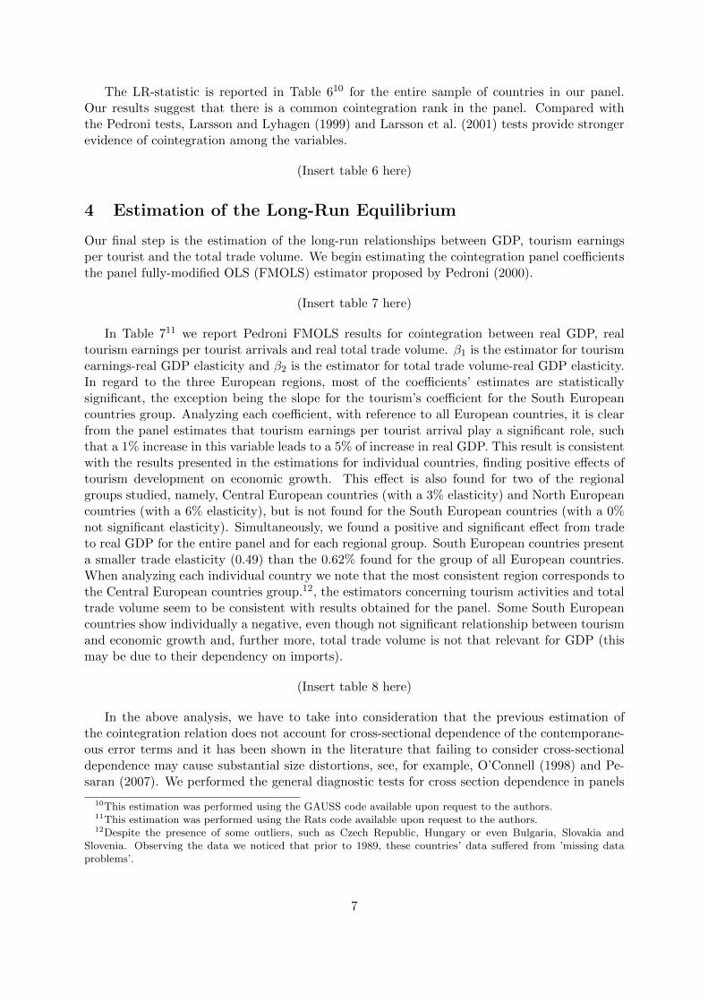
The LR-statistic is reported in Table 610 for the entire sample of countries in our panel.Our results suggest that there is a common cointegration rank in the panel. Compared withthe Pedroni tests, Larsson and Lyhagen (1999) and Larsson et al. (2001) tests provide strongerevidence of cointegration among the variables.


4 Estimation of the Long-Run Equilibrium

Our final step is the estimation of the long-run relationships between GDP, tourism earningsper tourist and the total trade volume. We begin estimating the cointegration panel coefficientsthe panel fully-modified OLS (FMOLS) estimator proposed by Pedroni (2000).


In Table 711 we report Pedroni FMOLS results for cointegration between real GDP, realtourism earnings per tourist arrivals and real total trade volume. β1 is the estimator for tourismearnings-real GDP elasticity and β2 is the estimator for total trade volume-real GDP elasticity.In regard to the three European regions, most of the coefficients’ estimates are statisticallysignificant, the exception being the slope for the tourism’s coefficient for the South Europeancountries group. Analyzing each coefficient, with reference to all European countries, it is clearfrom the panel estimates that tourism earnings per tourist arrival play a significant role, suchthat a 1% increase in this variable leads to a 5% of increase in real GDP. This result is consistentwith the results presented in the estimations for individual countries, finding positive effects oftourism development on economic growth. This effect is also found for two of the regionalgroups studied, namely, Central European countries (with a 3% elasticity) and North Europeancountries (with a 6% elasticity), but is not found for the South European countries (with a 0%not significant elasticity). Simultaneously, we found a positive and significant effect from tradeto real GDP for the entire panel and for each regional group. South European countries presenta smaller trade elasticity (0.49) than the 0.62% found for the group of all European countries.When analyzing each individual country we note that the most consistent region corresponds tothe Central European countries group.12, the estimators concerning tourism activities and totaltrade volume seem to be consistent with results obtained for the panel. Some South Europeancountries show individually a negative, even though not significant relationship between tourismand economic growth and, further more, total trade volume is not that relevant for GDP (thismay be due to their dependency on imports).


In the above analysis, we have to take into consideration that the previous estimation ofthe cointegration relation does not account for cross-sectional dependence of the contemporane-ous error terms and it has been shown in the literature that failing to consider cross-sectionaldependence may cause substantial size distortions, see, for example, O’Connell (1998) and Pe-saran (2007). We performed the general diagnostic tests for cross section dependence in panels

10This estimation was performed using the GAUSS code available upon request to the authors.11This estimation was performed using the Rats code available upon request to the authors.12Despite the presence of some outliers, such as Czech Republic, Hungary or even Bulgaria, Slovakia and

Slovenia. Observing the data we noticed that prior to 1989, these countries’ data suffered from ’missing dataproblems’.

7

suggested by Pesaran (2004) as shown in Tables 8-1113. The hypothesis that there are notcross-sectional dependence is rejected for all regions except for the South European countries.Therefore, we proceed to estimate our panel data model subject to error cross section depen-dence as suggested by Pesaran (2006). The Pesaran (2006)’s Monte Carlo simulations show thatcommon correlated effects-Pesaran (2006) pooled estimator (CCE-PPE) has satisfactory smallsample14 properties.



In Table 8 we present the estimation results for the pooled specification for the completesample as well as for each individual country. Removing the cross dependency, the estimator forthe tourism earnings by tourist arrival-GDP elasticity is around 0.5% although not significant.Total trade volume-GDP elasticity moves in opposite direction, augmenting its value towards92.2% for the set of all European countries. Maybe this result is due to the variable we areusing to measure external competitiveness: total trade volume. This variable also measurestourism flows because it contains the item travel and tourism from the current account. Thenwe are correlating GDP with tourism flows (inbound and outbound) whereas we are correlatingGDP with total trade volume. Regarding individual countries estimators, we find a similarperformance. The majority has no statistic significance and the values of the tourism earningsby tourist arrival-real GDP elasticities decreases as compared to the estimators obtained by theFMOLS methodology. Once more, total trade volume is the statistically significant variable andshowing generalized high magnitude estimators for its elasticities.


The same estimation technique: common correlated effects-Pesaran (2006) pooled estimator(CCE-PPE) applied to the three regional groups (see Tables 9, 10 and 11) provide similar resultsto the ones described to the all panel . We find larger coefficients for tourism-GDP elasticity forCentral European countries and North European countries when compared to South Europeancountries, but both are not statistically significant.

5 Conclusion

This paper showed that there is solid evidence of a panel cointegration relation between tourismand GDP in the European countries. As for the FMOLS estimates, the parameters had to beanalyzed carefully because we found the presence of common correlated effects. Removing thecross dependency, our panel tourism-led growth model indicates that tourism development hasa higher impact on GDP in the South than in North. Thus, for this group of countries, the beststrategy is to raise tourism receipts. Furthermore, and worth noting too, in general, the volumeof trade shows an increase in our sample economies and has significant effects on the economicgrowth rates.

AcknowledgementsWe are grateful to Francisco Camoes for useful comments, suggestions and support. We are alsothankful to Mohammad Hashem Pesaran, Johan Lyhagen and Takashi Yamagata for the GaussCodes and Peter Pedroni for the Rats Codes. Financial support from FCT, under UNIDE-ERCis also gratefully acknowledged.

13These estimations were performed using the GAUSS code available upon request to the authors.14Pesaran (2006)’s Monte Carlo simulations also showed that the mean group estimators (CCE-PMG) have

satisfactory properties when N and T are relatively large.

8

References

Balaguer, J. and Cantavella-Jorda, M. (2002), ‘Tourism as a long-run economic growth factor:the Spanish case’, Applied Economics 34, 877–884.

Banerjee, A. (1999), ‘Panel data unit roots and co-integration: an overview.’, Oxford Bulletinof Economics and Statistics 61(0), 607–629.

Bhagwati, J. and Srinivasan, T. (1979), Trade policy and development in international economicpolicy: theory and evidence, Johns Hopkins University Press, Baltimore, pp. 1–35.

Eugenio-Martin, J. (2004), Tourism and economic growth in latin-american countries: A paneldata approach, Nota di Lavoro 26, Fondazione Eni Enrico Mattei Working Paper Series.

Gunduz, L. and Hatemi-J., A. (2005), ‘Is the tourism-led growth hypothesis valid for Turkey?’,Applied Economics Letters 12, 499–504.

Helpman, E. and Krugman, P. R. (1985), Market Structure and Foreign Trade, The MIT Press,Cambridge, Massachussets.

Im, K. S., Pesaran, M. H. and Shin, Y. (2003), ‘Testing for unit roots in heterogeneous panels’,Journal of Econometrics 115, 53–74.

Johansen, S. (1995), Likelihood-based Inference in Co-integrated Vector Autoregressive Models,Oxford University Press, Oxford, UK.

Katircioglu, S. T. (2009), ‘Tourism, trade, and growth: the case of Cyprus’, Applied Economics41, 2741–2750.

Krueger, A. (1980), ‘Trade police as an input to development’, American Economic Review70, 188–292.

Larsson, R. and Lyhagen, J. (1999), Likelihood-based inference in multivariate panel cointegra-tion models, Working Paper 331, Stockholm School of Economics, Working paper series inEconomics and Finance.

Larsson, R., Lyhagen, J. and Lothgren, M. (2001), ‘Likelihood-based cointegration tests inheterogeneous panels’, Econometrics Journal 4(1), 109–42.

Lee, C. and Chang, C. (2008), ‘Tourism development and economic growth: A closer look atpanels’, Tourism Management 29, 180–192.

Levin, A., Lin, C.-F. and Chu, C.-S. J. (2002), ‘Unit root tests in panel data: asymptotic andfinite-sample properties’, Journal of Econometrics 108(1), 1–24.

McKinnon, R. (1964), ‘Foreign exchange constrain in economic development and efficient aidallocation’, Economic Journal 74, 388–409.

Moon, H. and Perron, B. (2004), ‘Testing for a unit root in panel with dynamic factors’, Journalof Econometrics 122, 81–126.

O’Connell, P. G. (1998), ‘The overvaluation of purchasing power parity’, Journal of InternationalEconomics 44(1), 1–19.

Oh, C. O. (2005), ‘The contribution of tourism development to economic growth in the Koreaneconomy’, Tourism Management 26, 39–44.

9

Pedroni, P. (1999), ‘Critical values for cointegration tests in heterogeneous panels with multipleregressors’, Oxford Bulletin of Economics and Statistics 61, 653–670.

Pedroni, P. (2000), Fully modified OLS for heterogeneous cointegrated panels in Advances inEconometrics: Vol. 15. Nonstationary Panels, Panel Cointegration, and Dynamic Panels.,JAI Press, Amsterdam, Holand, pp. 93–130.

Pedroni, P. (2001), ‘Purchasing power parity tests in cointegrated panels’, Review of Economicsand Statistics 83(4), 727–731.

Pedroni, P. (2004), ‘Panel cointegration; asymptotic and finite sample properties of pooled timeseries tests, with an application to the ppp hypothesis’, Econometric Theory 20(3), 597–625.

Pesaran, M. (2004), General diagnostic tests for cross section dependence in panels, WorkingPaper 1233, CESifo.

Pesaran, M. H. (2006), ‘Estimation and inference in large heterogeneous panel with a multifactorerror structure’, Econometrica 74(4), 967–1012.

Pesaran, M. H. (2007), ‘A simple panel unit root test in the presence of cross section dependence’,Journal of Applied Econometrics 22(446), 265–312.

10

Appendix

A DATA

Data used in this article are annual figures covering the period 1988-2010 and variables of this study are realGDP, tourism expenditures by tourist arrival, and real trade volume (total exports plus total imports). Data forGDP and total trade volume are taken from AMECO Database (Eurostat) and for tourism earnings and touristarrivals from World Travel and Tourism Council (WTTC). Variables, except tourist arrivals, were converted to2000 US$ constant prices using real exchange rates also taken from AMECO Database.

Data Sources

From the AMECO Database Eurostat, it was obtained:

GDP : GDP at current prices for the period 1988-2010.

INT : Total Trade Volume is total exports plus total imports for the period 1988-2010.

The World Travel and Tourism Council (WTTC) is the source of the following series:

TOUR: Number of production workers per industry, for the period 1988-2010.

11

Tables

Table 1: Panel Unit Root Tests

Tests GDP TOUR INTSeries in Log-Levels

All European Countries in the PanelLevin et al. (2002) Test -0.601 -0.916 -0.239Im et al. (2003) Test -0.677 -0.223 -0.063

Central European CountriesLevin et al. (2002) Test -0.694 -1.076 -0.534Im et al. (2003) IPS Test -0.482 -0.646 -0.849

North European CountriesLevin et al. (2002) Test -0.479 -1.076 -0.540Im et al. (2003) Test -0.403 -0.646 -0.893

South European CountriesLevin et al. (2002) Test 0.211 -0.537 0.176Im et al. (2003) Test -0.267 -0.222 0.748

The null hypothesis is that the series is a unit root process. An interceptand trend are included in the test equation. The lag length was selected byusing the Akaike Information Criteria. The critical values are taken fromfrom Im et al. (2003).

* Rejects the null at the 10% level.** Rejects the null at the 5% level.*** Rejects the null at the 1% level.

12

Table 2: Pesaran (2007) Cross-sectionally Augmented IPS (CIPS) Test

Lag p = 1 p = 2 p = 3

All European Countries in the PanelGDP -2.088* -1.797 -1.591TOUR -2.173* -1.843 -1.929INT -2.771** -2.208 -1.985

The null hypothesis is that the series is a unit root process. Critical values for theCIPS test are -3.35 (10%), -2.41 (5%), and -1.89 (1%), see Pesaran (2007).


Table 3: Moon and Perron (2004) Panel Unit Root Test

t∗a t∗b

All European Countries in the PanelGDP -0.020 -0.416TOUR -0.012 -0.062INT 0.076 1.631*

The tests statistics are distributed as N(0, 1) under the null of nonstationarity. Critical values are 1.28 (10%), 1.64 (5%) and 2.33(1%).


13

Table 4: Pedroni (2004) Panel Cointegration Tests

Test Statistic

All European Countries in the Panel -1.277*

Central European Countries -1.829*

North European Countries -0.241***

South European Countries -1.980*

The tests statistics are distributed as N(0, 1) under the null of nocointegration. The statistics are constructed using small sampleadjustment factors from Pedroni (1999, 2004).


14

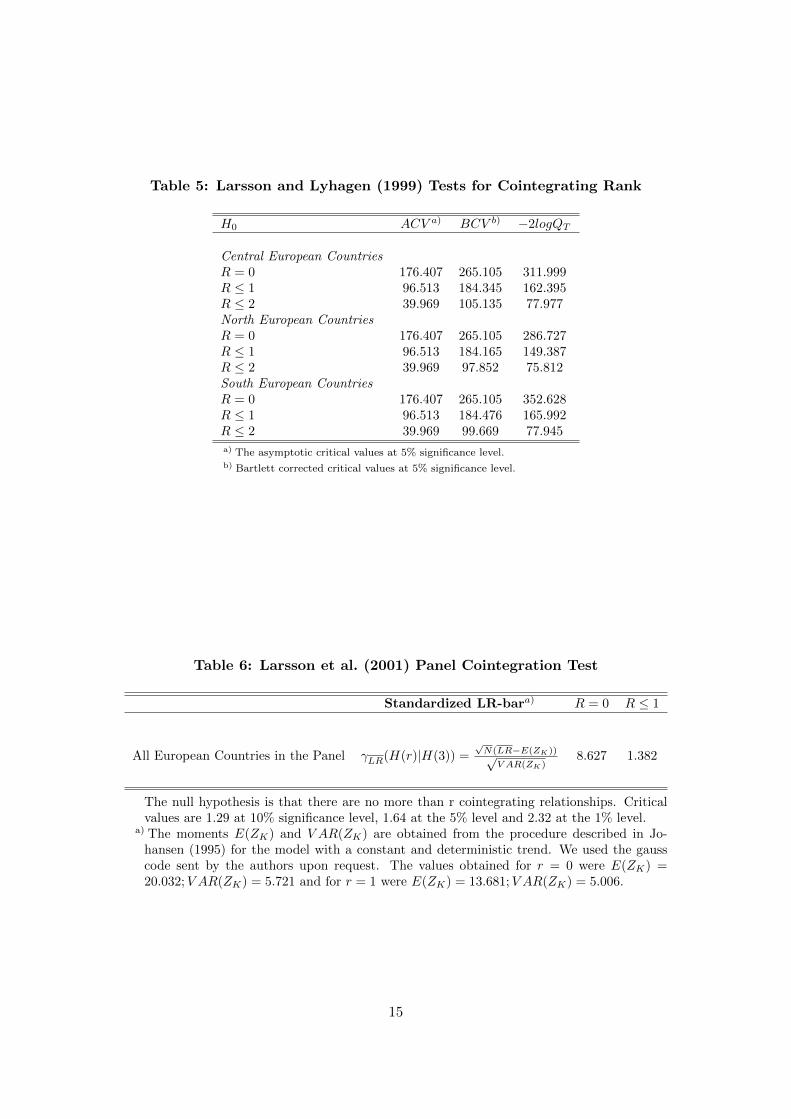
Table 5: Larsson and Lyhagen (1999) Tests for Cointegrating Rank

H0 ACV a) BCV b) −2logQT

Central European CountriesR = 0 176.407 265.105 311.999R ≤ 1 96.513 184.345 162.395R ≤ 2 39.969 105.135 77.977North European CountriesR = 0 176.407 265.105 286.727R ≤ 1 96.513 184.165 149.387R ≤ 2 39.969 97.852 75.812South European CountriesR = 0 176.407 265.105 352.628R ≤ 1 96.513 184.476 165.992R ≤ 2 39.969 99.669 77.945a) The asymptotic critical values at 5% significance level.b) Bartlett corrected critical values at 5% significance level.

Table 6: Larsson et al. (2001) Panel Cointegration Test

Standardized LR-bara) R = 0 R ≤ 1

All European Countries in the Panel γLR(H(r)|H(3)) =√N(LR−E(ZK))√

V AR(ZK)8.627 1.382

The null hypothesis is that there are no more than r cointegrating relationships. Criticalvalues are 1.29 at 10% significance level, 1.64 at the 5% level and 2.32 at the 1% level.

a) The moments E(ZK) and V AR(ZK) are obtained from the procedure described in Jo-hansen (1995) for the model with a constant and deterministic trend. We used the gausscode sent by the authors upon request. The values obtained for r = 0 were E(ZK) =20.032;V AR(ZK) = 5.721 and for r = 1 were E(ZK) = 13.681;V AR(ZK) = 5.006.

15

Table 7: Panel Estimates of the Cointegration Relationship: FMOLS

Panel Group FMOLS Results:β1 t-stat β2 t-stat

All European Countries 0.05 3.92*** 0.62 65.99***

Central European Countries 0.03 2.30*** 0.64 55.95***

South European Countries 0.00 -0.93 0.49 24.99***

North European Countries 0.06 3.39*** 0.69 30.37***

Countries Results:

β1 t-stat β2 t-statCentral European CountriesAustria 0.13 2.20*** 0.31 2.90***

Belgium 0.06 2.20*** 0.32 7.27***

Bulgaria -0.01 -0.36 1.06 57.90***

Czech Republic 0.33 3.87*** 0.72 5.33***

Germany 0.12 2.47*** 0.22 2.20***

Hungary -0.32 -6.37*** 0.83 11.08***

Luxembourg 0.06 1.20 0.58 5.47***

Netherlands 0.08 3.52*** 0.52 12.99***

Poland 0.23 2.77*** 0.94 15.04***

Romania 0.24 2.07 *** 0.99 46.83***

Slovakia 0.00 0.04 0.67 3.67***

Slovenia -0.03 -1.24 0.84 26.85***

Switzerland 0.04 1.35 0.33 3.32***

South European CountriesCyprus -0.05 -2.32 ***0.30 10.43***

France -0.03 -1.46 0.22 9.43Greece 0.51 2.75*** 0.93 4.80***

Italy -0.04 -0.54 0.24 1.91Malta 0.09 1.02 0.63 3.10Portugal -0.04 -0.54 0.24 1.91Spain -0.42 -1.50 0.02 0.07Turkey -0.06 -0.39 1.12 38.66***

North European CountriesDenmark 0.04 2.81*** 0.50 4.33***

Estonia 0.03 2.75*** 0.51 6.24***

Finland 0.08 0.67 0.80 5.32***

Iceland -0.03 -1.07 0.86 30.77***

Ireland -0.02 -0.20 0.51 5.19***

Latvia 0.10 4.09*** 0.63 3.26***

Lithuania 0.47 3.39*** 1.04 5.72***

Norway -0.07 -2.19*** 0.59 11.96***

Sweden 0.07 0.69 0.70 5.24***

UK -0.02 -0.23 0.74 18.03***

The tests statistics are distributed as N(0, 1) under the null of no-cointegration.The test statistics are constructed using small sample adjustment factors fromPedroni (2000, 2004).

*** Rejects the null at the 1% level.

16

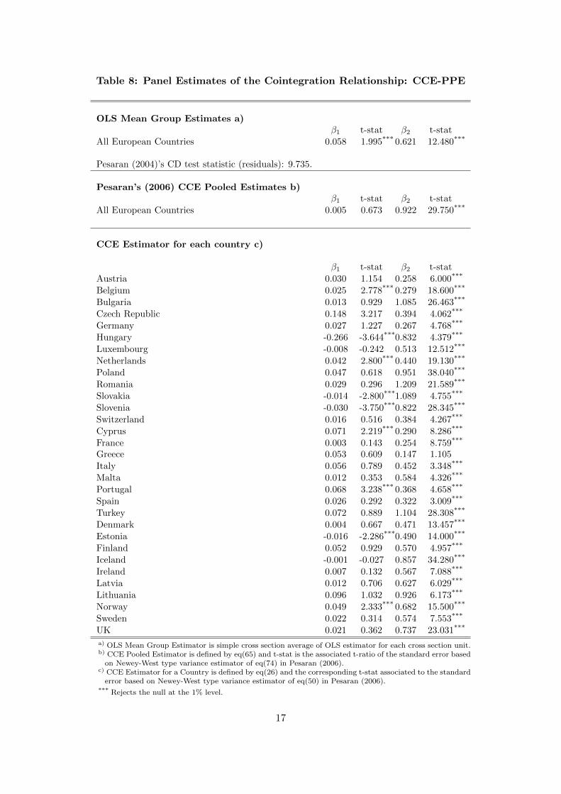
Table 8: Panel Estimates of the Cointegration Relationship: CCE-PPE

OLS Mean Group Estimates a)β1 t-stat β2 t-stat

All European Countries 0.058 1.995*** 0.621 12.480***

Pesaran (2004)’s CD test statistic (residuals): 9.735.

Pesaran’s (2006) CCE Pooled Estimates b)β1 t-stat β2 t-stat

All European Countries 0.005 0.673 0.922 29.750***

CCE Estimator for each country c)

β1 t-stat β2 t-statAustria 0.030 1.154 0.258 6.000***

Belgium 0.025 2.778*** 0.279 18.600***

Bulgaria 0.013 0.929 1.085 26.463***

Czech Republic 0.148 3.217 0.394 4.062***

Germany 0.027 1.227 0.267 4.768***

Hungary -0.266 -3.644***0.832 4.379***

Luxembourg -0.008 -0.242 0.513 12.512***

Netherlands 0.042 2.800*** 0.440 19.130***

Poland 0.047 0.618 0.951 38.040***

Romania 0.029 0.296 1.209 21.589***

Slovakia -0.014 -2.800***1.089 4.755***

Slovenia -0.030 -3.750***0.822 28.345***

Switzerland 0.016 0.516 0.384 4.267***

Cyprus 0.071 2.219*** 0.290 8.286***

France 0.003 0.143 0.254 8.759***

Greece 0.053 0.609 0.147 1.105Italy 0.056 0.789 0.452 3.348***

Malta 0.012 0.353 0.584 4.326***

Portugal 0.068 3.238*** 0.368 4.658***

Spain 0.026 0.292 0.322 3.009***

Turkey 0.072 0.889 1.104 28.308***

Denmark 0.004 0.667 0.471 13.457***

Estonia -0.016 -2.286***0.490 14.000***

Finland 0.052 0.929 0.570 4.957***

Iceland -0.001 -0.027 0.857 34.280***

Ireland 0.007 0.132 0.567 7.088***

Latvia 0.012 0.706 0.627 6.029***

Lithuania 0.096 1.032 0.926 6.173***

Norway 0.049 2.333*** 0.682 15.500***

Sweden 0.022 0.314 0.574 7.553***

UK 0.021 0.362 0.737 23.031***

a) OLS Mean Group Estimator is simple cross section average of OLS estimator for each cross section unit.b) CCE Pooled Estimator is defined by eq(65) and t-stat is the associated t-ratio of the standard error basedon Newey-West type variance estimator of eq(74) in Pesaran (2006).

c) CCE Estimator for a Country is defined by eq(26) and the corresponding t-stat associated to the standarderror based on Newey-West type variance estimator of eq(50) in Pesaran (2006).


17


Central European Countries


All Countries 0.065 1.585 0.649 8.269***



All Countries 0.006 1.120 0.974 50.576***


Central European Countries β1 t-stat β2 t-statAustria 0.023 1.211 0.430 3.071***

Belgium 0.002 0.167 0.550 8.333***

Bulgaria 0.011 1.222 0.959 31.967***

Czech Republic 0.042 0.700 0.473 4.637***

Germany 0.041 1.281 0.306 1.117Hungary -0.205 -8.542***1.113 23.188***

Luxembourg -0.020 -0.952 0.862 14.131***

Netherlands 0.010 0.714 0.701 18.946***

Poland 0.060 1.538 0.995 71.071***

Romania 0.073 1.217 1.130 35.313***

Slovakia -0.010 -2.500***0.900 4.390***

Slovenia -0.012 -3.000***0.899 64.214***

Switzerland 0.002 0.077 0.922 8.951***




18


South European Countries


All Countries 0.038 0.491 0.520 4.094***



All Countries 0.049 1.252 0.797 16.941***

CCE Estimator for each Country c)

South European Countries β1 t-stat β2 t-statCyprus 0.012 0.200 0.14 2.439***

France 0.046 0.767 0.20 3.736***

Greece 0.426 7.745*** 0.78 9.725***

Italy 0.030 0.909 0.95 11.321***

Malta 0.003 0.043 0.75 3.906***

Portugal 0.014 0.203 0.76 5.418***

Spain 0.009 0.214 0.85 8.455***

Turkey 0.046 0.407 0.88 16.509***

a) OLS Mean Group Estimator is simple cross section average of OLS estimator for each cross section unit.b) CCE Pooled Estimator is defined by eq(65) and t-stat is the associated t-ratio of the standard errorbased on Newey-West type variance estimator of eq(74) in Pesaran (2006).

c) CCE Estimator for a Country is defined by eq(26) and the corresponding t-stat associated to thestandard error based on Newey-West type variance estimator of eq(50) in Pesaran (2006).


19


North European Countries


All Countries 0.067 1.399 0.664 11.057***



All Countries 0.061 2.979*** 0.587 7.168***


North European Countries β1 t-stat β2 t-statDenmark 0.009 0.600 0.738 16.043***

Estonia 0.020 2.222 0.428 4.756***

Finland 0.152 2.027 0.426 2.731***

Iceland -0.019 -0.528 0.842 18.711***

Ireland 0.002 0.053 0.377 7.854***

Latvia -0.023 -2.556***-0.201 -4.467***

Lithuania 0.565 4.669*** 0.529 3.574***

Norway 0.017 0.895 0.514 9.885***

Sweden 0.095 2.436*** 0.170 2.297UK 0.030 0.577 0.629 22.464***




20

tourism and growth in european countries: an application

Documents