toward a flexible and reconfigurable …€¦ · 4 model partitions and dynamic repartitions in ......
TRANSCRIPT

TOWARD A FLEXIBLE AND RECONFIGURABLE DISTRIBUTED
SIMULATION: A NEW APPROACH TO DISTRIBUTED DEVS
by
Ming Zhang
_________________________
A Dissertation Submitted to the Faculty of the
DEPARTMENT OF ELECTRICAL AND COMPUTER ENGINEERING
In Partial Fulfillment of the Requirements
For the Degree of
DOCTOR OF PHILOSOPHY
In the Graduate College
THE UNIVERSITY OF ARIZONA
2007

2
THE UNIVERSITY OF ARIZONA
GRADUATE COLLEGE
As members of the Dissertation Committee, we certify that we have read the dissertation
prepared by Ming Zhang
entitled Toward a Flexible and Reconfigurable Distributed Simulation: A New Approach to Distributed
DEVS
and recommend that it be accepted as fulfilling the dissertation requirement for the
Degree of Doctor of Philosophy
_______________________________________________________________________ Date: 4/4/2007
Bernard P. Zeigler
_______________________________________________________________________ Date: 4/4/2007
Roman Lysecky
_______________________________________________________________________ Date: 4/4/2007
Janet Meiling Wang
Final approval and acceptance of this dissertation is contingent upon the candidate’s submission of the final
copies of the dissertation to the Graduate College.
I hereby certify that I have read this dissertation prepared under my direction and recommend that it be
accepted as fulfilling the dissertation requirement.
________________________________________________ Date: 4/4/2007
Dissertation Director: Bernard P. Zeigler

3
STATEMENT BY AUTHOR
This dissertation has been submitted in partial fulfillment of requirements for an
advanced degree at the University of Arizona and deposited in the University Library to
be made available to borrowers under rules of the Library.
Brief quotations from this dissertation are allowable without special permission, provided
that accurate acknowledgment of source made. Requests for permission for extended
quotation from or reproduction of this manuscript in whole or in part may be granted the
head of the major department or the Dean of the Graduate College when in his or her
judgment the proposed use of the material is in interests of scholarship. In all other
instances, however, permission must be obtained from the author.
SIGNED: Ming Zhang

4
ACKNOWLEDGEMENTS
I would like to express my greatest appreciation to my advisor Dr. Bernard P. Zeigler,
who introduced me to the fantastic world of discrete event simulation. His support and
encouragement on my research brought me so much insight which guides me to find my
way in the world of computer simulation.
I would like to thanks Dr. Phil Hammonds and Dr. James Nutaro for their help and
mentoring during my study.
I would like to thank Dr. Roman Lysecky and Dr. Janet Wang for serving as my defense
committee.
I would like to show special thanks to Ms. Lourdes Canto, who helps and supports me
during my graduate study.
I would like to thank all the members at ACIMS, especially Dr. Kim, Raj, Dr. Moon for
the useful discussion on my research.
Finally, I would like to express my wholehearted appreciation to my parents, who never
stop supporting and encouraging me.
5
DEDICATION
To
My Wife Yuanyuan

6
TABLE OF CONTENTS
LIST OF TABLES ............................................................................................................ 9
LIST OF FIGURES ........................................................................................................ 10
ABSTRACT..................................................................................................................... 12
1 INTRODUCTION .................................................................................................. 14
2 BACKGROUND..................................................................................................... 19
2.1 DEVS....................................................................................................... 19
2.1.1 Introduction of DEVS and DEVS Formalism .................................. 19
2.1.2 DEVS Modeling and Simulation Framework................................... 28
2.2 DEVSJAVA............................................................................................ 33
2.3 JAVA RMI ............................................................................................. 37
3 PARALLEL-DISTRIBUTED SIMULATION .................................................... 42
3.1 OVERVIEW........................................................................................... 42
3.2 DEVS BASED PARALLEL-DISTRIBUTED SIMULATION ......... 46
4 MODEL PARTITIONS AND DYNAMIC REPARTITIONS IN
DISTRIBUTED SIMULATION ENVIRONMENTS.................................................. 49
4.1 GENERAL MODEL PARTITION TECHNIQUE ............................ 49
4.2 MODEL PARTITION/REPARTITION IN DISTRIBUTED
SIMULATION FRAMEWORKS......................................................................... 55
5 DEVS/RMI—A NEW APPROACH TO DISTRIBUTED DEVS...................... 62
5.1 DEVS/RMI SYSTEM ARCHITECTURE .......................................... 62
5.2 SIMULATION CONTROLLER AND CONFIGURATION ENGINE
................................................................................................................. 65
5.3 SIMULATION MONITOR.................................................................. 68
5.4 REMOTE SIMULATORS.................................................................... 68
5.4.1 Remote Simulator Definition............................................................ 68
5.4.2 Remote Simulator Creation and Registration ................................... 69
5.4.3 Local Simulator vs. Remote Simulator............................................. 72

7
TABLE OF CONTENTS-Continued
5.5 DYNAMIC SIMULATOR AND MODEL MIGRATION................. 74
5.6 DYNAMIC MODEL RECONFIGURATION IN DISTRIBUTED
ENVIRONMENT ................................................................................................... 75
5.7 INCREASE LOCALITY FOR LARGE-SCALE CELL SPACE
MODEL IN DEVS/RMI......................................................................................... 76
5.8 BASIC PERFORMANCE TEST ......................................................... 78
6 MODEL PARTITIONS IN DEVS/RMI............................................................... 80
6.1 STATIC PARTITION........................................................................... 80
6.2 DYNAMIC REPARTITION ................................................................ 86
6.2.1 Overview........................................................................................... 86
6.2.2 A Dynamic Repartition Example...................................................... 88
7 INVESTIGATING THE COMPUTATION SPACE OF A SIMULATION
WITH DEVS/RMI .......................................................................................................... 95
7.1 INTRODUCTION ................................................................................. 95
7.2 SIMULATIONS OF CONTINUOUS SPATIAL MODELS.............. 97
7.3 HILLY TERRAIN MODEL................................................................. 98
7.4 WHY DEVS/RMI FOR HILLY TERRAIN MODEL ..................... 102
7.5 LINUX CLUSTER............................................................................... 104
7.6 MODEL PARTITION FOR HILLY TERRAIN MODEL.............. 104
7.7 AUTOMATIC TEST SETUP............................................................. 106
7.8 SPEEDUP OF SIMULATION FOR HILLY TERRAIN MODEL 108
7.9 SIMULATING VERY LARGE HILLY TERRAIN MODEL ........ 112
7.10 CONCLUSION .................................................................................... 112
8 LARGE-SCALE DISTRIBUTED AGENT BASED SIMULATION USING
DEVS/RMI..................................................................................................................... 114
8.1 DISTRIBUTED SIMULATION OF VALLEY FEVER MODEL.. 114
8.1.1 Valley Fever Model ........................................................................ 114

8
TABLE OF CONTENTS-Continued
8.1.2 Model Partition for Valley Fever Model ........................................ 115
8.1.3 Distributed Simulation Results for Valley Fever Model ................ 116
8.1.4 Workload Injection to the Distributed Cells ................................... 117
8.2 DYNAMIC RECONFIGURATION OF DISTRIBUTED
SIMULATION OF VALLEY FEVER MODEL USING ‘ACTIVITY’.......... 119
8.2.1 Introduction..................................................................................... 119
8.2.2 Static Blind Model Partition vs. Dynamic Reconfiguration Using
“Activity” ....................................................................................................... 120
8.2.3 Test Environment and Results ........................................................ 123
8.2.4 Discussion ....................................................................................... 125
9 CONCLUSION AND FUTURE WORK............................................................ 127
REFERENCES.............................................................................................................. 132

9
LIST OF TABLES
Table 6-1 Overhead Incurred by Dynamic Model Migration........................................... 93
Table 8-1 Distributed Simulation Execution Time for Static Blind Partition and Dynamic
Reconfiguration Using “Activity”—5 nodes. ................................................................. 124
Table 8-2 Distributed Simulation Execution Time for Static Blind Partition and Dynamic
Reconfiguration Using “Activity”—9 Nodes. ................................................................ 124

10
LIST OF FIGURES
Figure 2-1 Basic Entities and Relations [15] .................................................................... 21
Figure 2-2 Discrete Event Time Segments [1] ................................................................. 22
Figure 2-3 An Illustration For Classic DEVS Formalism [1]......................................... 24
Figure 2-4 DEVS Modeling and Simulation Framework [10] ........................................ 29
Figure 2-5 Coupled Modules Formed Via Coupling and Their Use As Components [10]
........................................................................................................................................... 30
Figure 2-6 Basic DEVS Simulation Protocol [10]........................................................... 31
Figure 2-7 DEVSJAVA Class hierarchy and main methods [11] ................................... 34
Figure 2-8 Simulate Hierarchical Coupled Model in Fast Mode [12] ............................. 35
Figure 2-9 RMI System [19]............................................................................................. 38
Figure 2-10 RMI in Action [20]........................................................................................ 40
Figure 4-1Activity Distribution and Associated Cost Tree [62]....................................... 56
Figure 4-2Decomposable Cost Tree [62].......................................................................... 56
Figure 4-3 Partition Tree [62] .......................................................................................... 57
Figure 4-4 Final Partition Result [62].............................................................................. 58
Figure 4-5 Dynamic Coupling Reconstruction[6] ............................................................ 59
Figure 4-6 Model Partition, Deployment and Simulation in DEVS/P2P[7].................... 61
Figure 5-1 DEVS/RMI System Architecture................................................................... 64
Figure 5-2 Flowchart of Distributed Simulation in DEVS/RMI ..................................... 67
Figure 5-3 Sequence Diagram for Creating Remote Simulators ..................................... 71
Figure 5-4 Local vs. Remote Simulator........................................................................... 73
Figure 5-5 Dynamic Simulator and Model Migration ..................................................... 74
Figure 5-6 Flowchart of Dynamic Coupling Changes..................................................... 76
Figure 5-7 Simple DEVS “gp” Model ............................................................................. 78
Figure 5-8 Messaging Overhead in Simple DEVS Model............................................... 79
Figure 6-1A Coupled DEVS Model ................................................................................. 81

11
LIST OF FIGURES-Continued
Figure 6-2A Random Partition Showing the Assignments of Atomic Models to
Computing Nodes ............................................................................................................. 83
Figure 6-3 2D Cell Space.................................................................................................. 83
Figure 6-4 Coupling Relationship Among Cells .............................................................. 84
Figure 6-5 Evenly Divided Sub-Domains of 2D Cell Space Model................................. 84
Figure 6-6 Irregular Re-Group the Cells to Different Computing Sub-Domains............. 86
Figure 6-7 Dynamic Model Repartition in DEVS/RMI .................................................. 88
Figure 6-8 A DEVS “gp” Model Before Model Repartition ........................................... 89
Figure 6-9 A DEVS “gp” Model After Model Repartition.............................................. 89
Figure 6-10 Dynamic Repartition in Action at USGS Beowulf Cluster-1 ...................... 90
Figure 6-11 Dynamic Repartition in Action at USGS Beowulf Cluster-2 ...................... 91
Figure 6-12 Sequence Diagram for Dynamic Model Migration...................................... 92
Figure 6-13 Overhead Incurred by Dynamic Model Repartitions ................................... 93
Figure 7-1 Calculate Hilliness and Traversed Time in 1D Space................................... 100
Figure 7-2 Calculate Hilliness in 2D Space................................................................... 101
Figure 7-3Hilly Terrain Model in Simview.................................................................... 102
Figure 7-4 Divided Hilly Terrain Model in Simview ..................................................... 106
Figure 7-5 Sequence Diagram for Automatic Setup Distributed Simulation ................. 107
Figure 7-6 Travel Time vs. Number of Cells................................................................. 109
Figure 7-7 Travel Time vs. Number of Hills ................................................................. 109
Figure 7-8 Speedup of Initialization Time with DEVS/RMI......................................... 110
Figure 7-9 Speedup of Simulation Using DEVS/RMI .................................................. 111
Figure 8-1Valley Fever Model in DEVSJAVA SimView.............................................. 115
Figure 8-2 Simulation Execution Time(seconds) vs. No. of Computing Nodes in Original
Model .............................................................................................................................. 117
Figure 8-3 Simulation Execution Time(seconds) vs. No. of Computing nodes Under
Different Workload on Distributed Cells........................................................................ 118
Figure 8-4 Selecting High-Activity Cells ....................................................................... 122

12
ABSTRACT
With the increased demand for distributed simulation to support large-scale
modeling and simulation applications, much research has focused on developing a
suitable framework to support simulation across a heterogeneous computing network.
Middleware based solutions have dominated this area for years, however, they lack the
flexibility for model partitions and dynamic repartition due to their innate static natures.
In this dissertation, a novel approach for DEVS based distributed simulation framework
is proposed and implemented. The objective of such a framework is to distribute
simulation entities across network nodes seamlessly without any of the commonly used
middleware, as well as to support adaptive and reconfigurable simulations during run-
time. This new approach, called DEVS/RMI, is proved to be well suited for complex,
computationally intensive simulation applications and its flexibility in a distributed
computing environment promotes a rapid development of distributed simulation
applications. A hilly terrain continuous spatial model is studied to show how DEVS/RMI
can easily refactor the simulations to accommodate both increases of the resolution and
computation nodes. Furthermore, an agent-based valley fever model is investigated in
this dissertation with particular interests on the concept of DEVS “activity”. Dynamic
reconfiguration of distributed simulation is then exemplified using the “activity” based
model repartition in a DEVS/RMI supported environment. The flexibility and
reconfigurable nature of DEVS/RMI open up further investigations into the relationship

13
between speedup of a simulation and the partition or repartition algorithm used in a
distributed simulation environment.

14
1 INTRODUCTION
Discrete Event System Specification (DEVS) is a mathematical formalism [1] to
describe real-world system behaviors in an abstract and rigorous manner. DEVS has
defined its standard as a well-known discrete event modeling and simulation
methodology. Compared with Non-DEVS traditional modeling and simulation
methodologies, DEVS defines a strict and concrete modeling and simulation framework
that supports fully object oriented modeling and simulation. Furthermore, DEVS has
been proved to be effective not only for discrete event models but also for continuous
spatial and hybrid models. With the help of modern object oriented language such as C++
and Java, the frameworks for modeling and simulation based on DEVS have reached
their mature stages and have been applied in many real-world applications.
With the increased demand for high-performance and large-scale simulation
frameworks, parallel and distributed simulations are called on to support various
scientific and engineering studies, including technical (e.g., standards conformance),
system level (focus on a single natural or engineered system) and operational (focus on
multiple systems, such as families of systems or system of systems) [2]. The objectives of
such studies may include testing of correctness of system behavior/function, evaluation of
measures of performance, and evaluation of measures of effectiveness and key
performance parameters. An ideal parallel and distributed framework should be able to
meet the following requirements:

15
• Flexibility – must handle a wide range of dynamic, information exchange and
dialogic behaviors.
• Institutionalized Reuse – support for model reuse and composability, not only at
the syntactical, but at the semantic and pragmatic levels as well.
• Model Continuity – allow basic development of systems in virtual time-managed
mode, while supporting stage-wise transition to real-time hardware in the loop
implementation as well.
• Quality of Service – should provide acceptable simulation performance at
minimum, and increased performance in dimensions such as execution time when
required.
With regard to parallel-distributed DEVS frameworks, there have been noticeable
progresses in recent years. DEVS/C++ [3], ADEVS [4] and CD++ [5] are such software
tools that work well for shared memory multi-processors, and have been used to simulate
large-scale models in practice. These implementations provide the necessary power for
high-performance parallel-distributed simulation, but lack the flexibilities for mapping
models to processors. Other DEVS based parallel-distributed simulation frameworks
include DEVS/GRID [6], DEVS/P2P [7], DEVS/HLA [8], DEVS/CORBA [9] and etc.,
which use middleware to bridge the simulation entities with the underlying networks, and
therefore, only limited support for model distribution is provided in a networking
environment.

16
In this dissertation, a new distributed DEVS modeling and simulation framework,
called DEVS/RMI [2], is proposed and implemented. DEVS/RMI is a significant
extension of DEVS/JAVA [11] and aims to provide a simulation framework which can
easily scale a single machine's simulation to multiple distributed processors. It is an
integration of Java RMI [13] technology with DEVS/JAVA, and is able to transparently
distribute simulation entities (models and/or simulators) to cluster of machines, which
greatly reduces the difficulties of mapping partitioned models to computing processors.
Because Java RMI supports the synchronization of local objects with remote ones, no
additional simulation time management, beyond that already in DEVSJAVA, needs to be
added when distributing the simulators to remote nodes. It also provides an auto-adaptive
and reconfigurable environment for dynamic model re-partition and simulator/model
migration. Such an environment simplifies simulator/model distribution across a network
without the help of other middleware while still providing platform independence
through the use of Java and its Virtual Machine (JVM) implementations. Compared with
other implementations using traditional high performance computing environments such
as MPI or PVM, DEVS/RMI provides a flexible and efficient software development
environment for rapid development of distributed simulation applications. The approach
using DEVS/RMI is tested and verified in this dissertation to be well suited for complex,
computationally intensive, and dynamic simulation applications. We need the high-
performance capabilities to address the computational complexity needed to thoroughly
examine complex natural systems and also to test and certify trusted information systems.
Therefore, the approach of DEVS/RMI presented in this dissertation opens a wide area of

17
simulation research, and it also helps promoting science and engineering studies by
providing a high performance and flexible distributed simulation framework.
In terms of some of the application areas, DEVS/RMI could be easily applied to
refactor simulation applications in a circumstance when both problem sizes and
computation nodes need increase. It is an ideal simulation framework for investigating
the computation space for large-scale continuous spatial models in which the resolution
of the simulation needs to be adjusted by increasing or decreasing the cell-space sizes.
Furthermore, the capability of DEVS/RMI to support dynamic reconfiguration of
simulations will help the study of behaviors of very large-scale dynamic system, where
both the flexibility of model partitions and the necessary computing power are on-
demand. DEVS/RMI could also be run on a Grid environment natively as long as JVM is
installed on the participating computing nodes. Such a capability to scale a single
machine’s simulation to a large-scale Grid computing environment makes the
DEVS/RMI more attractive for a wide area of applications including large-scale agent-
based simulation, computing intensive simulation testing and etc.
The main contributions of this dissertation are as follows:
• Designed and implemented a scalable and flexible distributed simulation
framework called DEVS/RMI.
• Studied the computation space of a large-scale continuous spatial hilly terrain
model with the help of DEVS/RMI.

18
• Studied and implemented “activity” based dynamic reconfiguration in a
distributed simulation environment.
The organization of this dissertation is described as followings: Chapter 2
presents some background information directly related to this dissertation, where basic
DEVS theory and formalism are briefly reviewed. DEVSJAVA and JAVA RMI are both
discussed to provide necessary links for later Chapters. Chapter 3 reviews the principle
concepts and research in parallel and distributed simulation, and Chapter 4 reviews the
model partition and dynamic repartition techniques commonly used in the distributed
simulation circumstances. Chapter 5 proposes the design and implementation of
DEVS/RMI, where the key attributes of it are presented and discussed in detail. Chapter 6
presents the model partition technique implemented in DEVS/RMI followed by Chapter
7, which investigated and demonstrated how DEVS/RMI can be applied on the study of
computational space of large-scale continuous special model. Chapter 8 shows the
effectiveness of DEVS/RMI on solving large-scale agent based model as well as dynamic
reconfiguration capability using model “activity”. At last, Chapter 9 discusses the
performance issues related to DEVS/RMI, and the dissertation is then concluded by
Chapter 10 which also suggests some future works.

19
2 BACKGROUND
2.1 DEVS
2.1.1 Introduction of DEVS and DEVS Formalism
Discrete Event System Specification (DEVS) is a mathematical formalism to
describe real-world system behavior in an abstract and rigorous manner. Compared with
traditional methodology for modeling and simulation, DEVS formalism describes and
specifies a modeled system as a mathematical object, and such object based
representation of the targeted system can then be implemented using different simulation
languages, especially modern object-oriented ones. In general, a system has a set of key
parameters when being modeled in a modeling framework, which include time base,
inputs, states, outputs, and functions for determining state transitions. Discrete event
systems in general encapsulate these parameters as object entities, and then use modern
object oriented simulation languages to describe the relationship among the specified
entities. As a pioneering formal modeling and simulation methodology, DEVS provides a
concrete simulation theoretical foundation, which promotes fully object-oriented
modeling and simulation techniques for solving today’s simulation problems required by
other science and engineering discipline. The insight provided by the DEVS formalism is
in the simple way that it characterizes how discrete event simulation languages specify
discrete event system parameters [14]. Having such an abstraction, it is possible to design
new simulation languages with sound semantics that are easier to understand than
traditional ones. Figure 2-1 presents a DEVS concept framework to show the basic
20
objects and their relationships in a DEVS modeling and simulation world. These basic
objects include [15]:
• the real system, in existence or proposed, which is regarded as fundamentally a
source of data
• model, which is a set of instructions for generating data comparable to that
observable in the real system. The structure of the model is its set of instructions.
The behavior of the model is the set of all possible data that can be generated by
faithfully executing the model instructions.
• simulator, which exercises the model's instructions to actually generate its
behavior.
• experimental frame, which captures how the modeler’s objectives impact on
model construction, experimentation and validation. As implemented in
DEVJAVA, such experimental frames are formulated as model objects in the
same manner as the models of primary interest. In this way, model/experimental
frame pairs form coupled model objects with the same properties as other objects
of this kind. It will become evident later, that this uniform treatment yields
immediate benefits in terms of modularity and system entity structure
representation.
These basic objects are then related by two relations [15]:
• modeling relation: linking real system and model, defines how well the model
represents the system or entity being modeled. In general terms a model can be

21
considered valid if the data generated by the model agrees with the data
produced by the real system in an experimental frame of interest.
• simulation relation, linking model and simulator, represents how faithfully the
simulator is able to carry out the instructions of the model.
Source
System
Simulator
Model
Experimental Frame
Simulation
Relation
Modeling
Relation
behavior database
Figure 2-1 Basic Entities and Relations [15]
In the view from DEVS, the basic items of data produced by a system or model
are time segments. These time segments are mappings from intervals defined over a
specified time base to values in the ranges of one or more variables [15]. These variables
can either be observed or measured. An example of a data segment is shown in Figure
2-2, where X is inputs, S is states, e is time elapsed, and Y is outputs.

22
x0 x1X
S
Y
y0
e
t0 t1 t2
Figure 2-2 Discrete Event Time Segments [1]
In fact, DEVS formalism provides a formal definition to describe the data
segment depicted above in Figure 2-2, and the history of DEVS can be traced back to
decades ago. A standard and classic DEVS formalism is defined as a structure [1]:
M = <X, S, Y, δint, δext, λ, ta>
where,
X : set of inputs;
S : set of states;
Y : set of outputs;
δint: S → S : internal transition function
δext : Q × X → S : external transition function

23
Q = { (s,e) | s ∈ S, 0 ≤ e ≤ ta(s) } is the set of total states where e is the
elapsed time since last state transition.
λ : S → Y : output function
ta : S → +
∞,0R : time advance function;
Figure 2-3 illustrates the key concept of above classic DEVS formalism.
Assuming the system is in state S after a previous state transition, it will stay in state S
for a duration determined by ta(s). When this resting time of ta() expires(or say the
elapsed time e=ta(s)), the system gives output λ(s) and changes its state from s to s’. This
state transition is exactly determined by the internal transition function δint as mentioned
in the formalism. However, if an external event occurs through the input X before the
duration specified by ta(s)(or say, the system is in total state (s,e) with e= ta(s), the
system will change to a state determined by δext(s,e,x) . After the system changes its state
to a new state, the same rules in the formalism are applied to govern how the system
responses to discrete events. DEVS makes an explicit difference between internal and
external state transitions, where the internal transition function determines the system’s
new state when no events have occurred since the last transition, while the external
transition function determines the system’s new state when an external event occurs
between 0 and ta(s). It is worth to note that ta(s) is a real number including 0 and ∞,
where “0” means that the system is a so-called “transitory” state that no external events
can intervene, and “∞” means that the system is in a so-called “passive” state that is
unchanged forever until an external event wakes it up.

24
Figure 2-3 An Illustration For Classic DEVS Formalism [1]
The above classic DEVS formalism does not take into account of concurrent
events, and therefore, has relatively limited usage for real-world application. With the
consideration of concurrent events and parallel processing on a discrete event system,
parallel DEVS system specification is developed from classic DEVS. The key
capabilities of Parallel DEVS beyond the classical DEVS are [1]:
• Ports are represented explicitly – there can be any of input and output ports on
which values can be received and sent.
• Instead of receiving a single input or sending a single output, basic parallel DEVS
models can handle bags of inputs and outputs. It should be noted here that a bag
can contain many elements with possibly multiple occurrences of its elements.

25
• A transition function, called confluent, is added, which decides the next state in
cases of collision between external and internal events.
Such parallel DEVS formalism consists of two parts: basic and coupled models.
A basic model of a standard parallel DEVS is a structure [1]:
M = <XM, S, YM, δint, δext, δcon, λ, ta>
where,
XM ={( p , v) | p∈IPorts, v∈Xp } is the set of input ports and values;
YM ={( p , v) | p∈OPorts, v∈Yp } is the set of output ports and values;
S : set of sequential states;
δint: S → S : internal transition function
δext : Q × XMb → S : external transition function
δcon: Q × XMb → S : confluent transition function
XMb is a set of bags over elements in X,
λ : S → Yb : output function generating external events at the
output;
ta : S → +
∞,0R : time advance function;
Q = { (s,e) | s ∈ S, 0 ≤ e ≤ ta(s) } is the set of total states where e is the
elapsed time since last state transition.
Such basic model as defined in parallel DEVS captures the following information
from a discrete event system:

26
� the set of input ports through which external events are received
� the set of output ports through which external events are sent
� the set of state variables and parameters
� the time advance function which controls the timing of internal transitions
� the internal transition function which specifies to which next state the system will
transit after the time given by the time advance function has elapsed
� the external transition function which specifies how the system changes state
when an input is received. The next state is computed on the basis of the present
state, the input port and value of the external event, and the time that has elapsed
in the current state.
� the confluent transition function which decides the next state in cases of collision
between internal and external events.
� the output function which generates an external output just before an internal
transition takes place.
Basic model is a building block for a more complex coupled model, which defines
a new model constructed by connecting basic model components. Two major activities
involved in coupled models are specifying its component models and defining the
couplings which create the desired communication networks. A coupled model is defined
as follows [1]:
DN = <X, Y, D, {Mi}, {Ii}, {Zi,j}>
where,

27
X : set of external input events;
Y : a set of outputs;
D : a set of components names;
for each i in D,
Mi is a component model
Ii is the set of influencees for i
for each j in Ii,
Zi,j is the i-to-j output translation function
A coupled model template captures the following information:
� the set of components
� for each component, its influencees
� the set of input ports through which external events are received
� the set of output ports through which external events are sent
� the coupling specification consisting of:
o the external input coupling (EIC) connects the input ports of the coupled
to one or more of the input ports of the components
o the external output coupling (EOC) connects the output ports of the
components to one or more of the output ports of the coupled model
o internal coupling (IC) connects output ports of components to input ports
of other components

28
As we have seen in this section, DEVS formalisms are strictly defined and it
evolves continuously to satisfy the requirement of today’s large and complex system
modeling and simulation. It has been extended by a lot of researcher around world,
however, its core concept is unchanged as we can see from the classic and parallel
formalisms. In the next section, we will discuss DEVS modeling framework and
simulation protocol, which provides the keys to the understanding of this dissertation’s
goal.
2.1.2 DEVS Modeling and Simulation Framework
DEVS modeling and simulation framework is very different with traditional
module and function based ones. It provides a very flexible and scalable modeling and
simulation foundation by separating models and simulators. Figure 2-4 shows how
DEVS model components interact with DEVS and Non-DEVS simulators through DEVS
simulation protocol. We can also see that DEVS models interact with each other through
DEVS simulators. The separation of models from simulators is a key aspect in the DEVS,
which is critical for scalable simulation and middleware supported distributed simulation
such as those using CORBA, HLA, and MPI.

29
Figure 2-4 DEVS Modeling and Simulation Framework [10]
The advantages for such a framework is obvious because model development is in
fact not affected by underlying computational resources for executing the model.
Therefore, models maintain their reusability and can be stored or retrieved from a model
repository. The same model system can be executed in different ways using different
DEVS simulation protocols. In such a setting, commonly used middleware technologies
for parallel and distributed computing could be easily applied on separately developed
DEVS models. Therefore, within the DEVS framework, model components can be easily
migrated from single processor to multiprocessor and vice versa.
If we have a closer look at DEVS based modeling framework, we will find that it
is based on hierarchical model construction technique as shown on Figure 2-5. For
instance, a coupled model is obtained by adding a coupling specification to a set of
atomic models. This coupled model can then be used as a component in a larger system
with new components. A hierarchical coupled model can be built level by level by adding
Simulator
Single
processor
Distributed
Simulator
Real-Time
Simulator
C++
Non
DEVS
DEVS
Java
Other
Representation
DEVS
Simulation
Protocol

30
a set of model components (either atomic or coupled) as well as coupling information
among these components. Reusable model repository for developers is therefore created.
DEVS based modeling framework also supports model component as a “blackbox”,
where the internals of the model is hidden and only the behavior of it is seen through its
input/output ports.
One interesting aspect of DEVS formalism is that a coupled DEVS model can be
expressed as an equivalent basic model (or say atomic model). This attributes in DEVS
formalism is so-called closure under coupling. Such a equivalent basic model transferred
from a coupled model can then be employed in a larger coupled model. Therefore, DEVS
formalism provides an excellent composition framework that supports closure under
coupling and hierarchical construction.
Atomic
Atomic
Atomic
Atomic
+ coupling
hierarchical
construction
Atomic
A tomic
A tomic
Figure 2-5 Coupled Modules Formed Via Coupling and Their Use As Components [10]
31
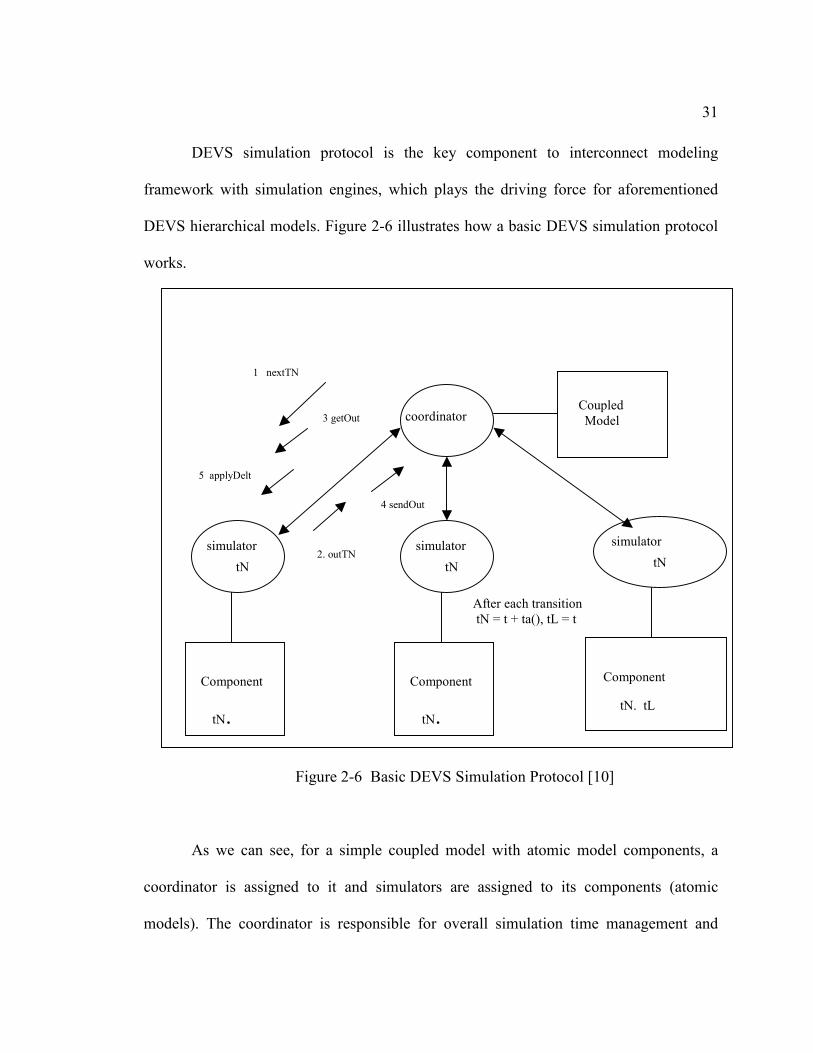
DEVS simulation protocol is the key component to interconnect modeling
framework with simulation engines, which plays the driving force for aforementioned
DEVS hierarchical models. Figure 2-6 illustrates how a basic DEVS simulation protocol
works.
Figure 2-6 Basic DEVS Simulation Protocol [10]
As we can see, for a simple coupled model with atomic model components, a
coordinator is assigned to it and simulators are assigned to its components (atomic
models). The coordinator is responsible for overall simulation time management and
coordinator
simulator
Component
tN
tN.
After each transition
tN = t + ta(), tL = t
simulator
Component
tN
tN.
simulator
Component
tN
tN. tL
Coupled
Model
1 nextTN
2. outTN
3 getOut
4 sendOut
5 applyDelt

32
execution. At each simulation step controlled by coordinator, each simulator reacts to the
incoming message as follows [10]:
(1). Coordinator sends nextTN to request tN from each of the simulators.
(2). All the simulators reply with their tNs in the outTN message to the
coordinator.
(3). Coordinator sends to each simulator a getOut message containing the global tN
(the minimum of the tNs)
(4) . Each simulator checks if it is imminent (its tN = global tN) and if so, returns the
output of its model in a message to the coordinator in a sendOut message. If it is
imminent and its input message is empty, then it invokes its model’s internal
transition function; If it is imminent and its input message is not empty, it invokes
its model’s confluence transition function; If is not imminent and its input
message is not empty, it invokes its model’s external transition function; If is not
imminent and its input message is empty then nothing happens.
(5) Coordinator uses the coupling specification to distribute the outputs as
accumulated messages back to the simulators in an applyDelt message to the
simulators – for those simulators not receiving any input, the messages sent are
empty.
The basic DEVS simulation protocol demonstrated above provides a core concept
on how DEVS drives the simulators as well as how simulators inter-actions with model
components. In fact, other DEVS simulation protocols use the key concept of the basic

33
protocol with added extensions for dealing with different circumstances. In general,
DEVS based framework supports hierarchical, modular based modeling and simulation
using reusable model components, and it can take a full range of computational methods
to support scalable and flexible modeling and simulations including distributed and real-
time based solutions.
In the subsequent section, DEVSJAVA, a known implementation of parallel
DEVS formalism, is reviewed with the focus on how the simulation protocol is
implemented in it.
2.2 DEVSJAVA
DEVSJAVA [11] is an implementation in Java of DEVS framework that has been
used for solving real-world simulation problem as well as serving as an openly available
teaching tool. It is a fully object orient implementation of standard parallel DEVS
formalism, and therefore, provides a very dynamic and flexible modeling and simulation
framework. DEVSJAVA has relatively complex class hierarchical structure, and it is the
foundation of DEVS/RMI, which is a distributed DEVS proposed and implemented in
this dissertation.
Figure 2-7 illustrated a somewhat simplified class hierarchy diagram implemented
in DEVSJAVA, where devs, is the base class of the DEVS sub-hierarchy with Atomic
and Coupled as the main derived classes of it [11]. Class digraph is a main subclass of
class coupled to define coupled model as described in previous subsection. For DEVS
model developers, the user-defined model classes should derive from these basic classes
and such model classes then become new components in DEVS for later reuse. The

34
implementation of DEVSJAVA supports the fundamental concept of DEVS hierarchical
construction and makes it easier to build complex model.
Figure 2-7 DEVSJAVA Class hierarchy and main methods [11]
Class message is derived from the container class and it encapsulates the data that
needs to be transferred back and forth among components in a coupled model. A message
consists of (port, value) pair, where value actually carries an entity instance transmitted
from sender to receiver. Because value derives from entity class, any entity can be
transmitted across involved simulators. Since model component is devs class instance,

35
and devs is a derived class of entity, model itself can be transmitted from one component
to another!
DEVSJAVA has a well-defined class hierarchical structure as we have seen.
Now, we will look at its simulation protocol and understand how it works. In fact, its
simulation engine actually implements and extends the basic DEVS simulation protocol
aforementioned.
Figure 2-8 Simulate Hierarchical Coupled Model in Fast Mode [12]
We focus our discuss on how DEVSJAVA simulator protocol works in its fast
mode, which is a generally used simulation mode for gaining fastest simulation speed. As
shown in Figure 2-8, in DEVSJAVA, the coordinator is the main and overall simulation
Coordinator
Coupled-
Coordinator
Coupled-
Simulator4
Ato
mic4
Coupled-
Simulator3
Ato
mic3
simulators.tellAll("initialize“)
simulators.AskAll(“nextTN”)
simulators.tellAll("computeInputOu
tput“)
simulators.tellAll("sendMessages")
simulators.tellAll("DeltFunc“)
putMessage putMessage
putMessage
Coupled-
Simulator1
Coupled-
Simulator2
Ato
mic1
Ato
mic2
putMessage
putMyMessage
Couple
d1
sendDownMessage

36
control thread which governs the whole simulation execution. Initially, the model is
passed to the coordinator, which then decomposes the model according to its hierarchical
structure. In such a way, each atomic model is assigned a CoupledSimulator, while each
coupled model is assigned a CoupledCoordinator. A CoupledCoordinator combines the
functionality of a CoupledSimulator and a coordinator. It works as a CoupledSimulator
to its peer brothers (such as CoupledSimulator3 and CoupledSimulator4 in Figure 2-8), to
which messages are sent by calling each other’s putMessage() function. However, it
works as a coordinator to its children ( such as CoupledSimulator1 and
CoupledSimulator2 in Figure 2-8). As an example, if CoupledCoordinator gets external
input from CoupledSimulator3 or CoupledSimulator4, it calls its sendDownMessage() to
send the message down to its children (CoupledSimulator1) based on the
internalModelTosim data structure explained below. On the other hand, if Atomic2
generates output, CoupledSimulator2 then calls CoupledCoordinator’s putMyMessage()
to put the message to CoupledCoordinator’s output port, which then puts the message to
CoupledSimulator3’s input port.
In this section, we have briefly reviewed some of the background of DEVSJAVA
class hierarchy and how simulation protocol works in it. In the next section, we will look
into the Java RMI, which is key technology used in this dissertation for developing a
fully dynamic distributed simulation framework.

37
2.3 JAVA RMI
Distributed object computing is an emerging technology that helps on solving
large-scale computing problems in a distributed network environment in a transparent
way. A software system built on distributed objects has many advantages over traditional
parallel and distributed computing techniques, such as:
• Maintaining the original object architecture built for a single processor, which is
important for building large-scale scalable system.
• Task or computing workload distribution is at object level, which helps on solving
load-balance, fault-tolerance problems in distributed computing in an easier way.
• Make the design of highly dynamic and reconfigrable distributed framework
easier.
• Systems integration can be performed to a higher degree.
The major representatives for distributed object technologies include Java RMI,
CORBA [16], DCOM [17]and .NET Remote [18]. CORBA is developed by Object
Management Group (OMG) and is a distributed framwork supporting inter-language
objects linked by CORBA Object Request Broker (ORB). DCOM and .NET Remote are
Microsoft’s implementations for distributed objects computing, which are mostly relied
on Microsoft Windows Operating System, although Unix based support has been
proposed and implemented recently.
Java Remote Method Invocation (RMI) [13] is Sun Java’s answer to distributed
object computing technology, which allows Java objects to be distributed across a

38
heterogeneous network. Its high level abstraction of message passing in a heterogeneous
network simplifies distributed computing system designs and implementations. Java RMI
hides all low-level communication handling from the programmers and combines local
and remote objects references in a same program context, where remote objects uses a
stub class (the proxy for remote object) to interact with other local objects.
Figure 2-9 RMI System [19]
A JAVA RMI system is a multi-layered structure as shown in Figure 2-9, where a
client and a server interact with each other through these layers [19]. The first layer is the
RMI Stub/Skeleton Layer, which is responsible for managing the remote object interface
between the client and server. The second layer is the Remote Reference Layer (RRL),
which manages the references of the remote objects. The third layer is the transport layer

39
that handles the lower level data communications. In common cases, the transport layer is
implemented with TCP/IP based Java Remote Method Protocol (JRMP).
In the RMI programming model, a RMI server defines a set of remote objects and
methods that clients can invoke remotely. These remote methods have to be declared in
an interface, which is used by client’s stub for type checking and casting. As a complete
distributed object framework, Java RMI relies on several key components/techniques :
• RMI Registry: a daemon Java server application which holds information
about available server objects. It acts as a central management point for
RMI system and actually a simple name repository. It generally runs on
certain port at server machine, for example, the default running port is:
1099.
• Remote Object Lookup: A RMI client uses RMI URL to locate demanding
remote object references, which are stored in the server RMI Registry.
• Stubs and Skeletons: proxy classes generated by rmic compiler to
help on transparent objects communications among local and remote
Java objects. In general, the stub resides on the client machine and
the skeleton resides on the server machine.
• Object Serialization: a key techniques used in RMI system, used for
transmit Java object across wire in a distributed computing environment.
Any Java object transmitted by RMI procedure has to be a serialized, which
allows objects to be marshaled (or transmitted) as a stream.

40
Java RMI is a powerful and flexible technology to support fully object level
architecture. It supports client-server programming model with the advantage of object
migration across network. Such object level transmitting provides more power than
traditional remote procedure call and it helps on designing and implementing a scalable
distributed system much easier.
Figure 2-10 RMI in Action [20]
Figure 2-10 depicts an acting RMI system, where RMI server binds a name with a
remote object and then registers this name to rmiregistry; RMI client lookups the
rmiregistry to locate the remote object before initiating any remote method calls. The
RMI server can also interact with web server directly using URL protocol for loading
class definition on demand.
Compared with CORBA and DCOM, JAVA RMI is a Java-specific middleware,
hence there are no separate IDL mappings as required by DCOM or CORBA. Java-RMI
can work with true sub-classes, while DCOM and CORBA can not do since they are
static object models. JAVA RMI supports dynamic class loading as well as distributed
garbage collection, which makes it unique for building very flexible and dynamic

41
distributed system. However, the confinement to Java language and network latency for
RMI procedure have to be carefully considered when constructing a large-scale
distributed RMI system.
The performance of RMI [21] has attracted many researchers for years. The major
drawback of Sun’s RMI implementation is the communication latency due to the
inefficient object serialization and marshalling. However, some other high performance
RMI implementations, such as Manta RMI [22], KaRMI [23], have been developed in
recent years, which make RMI a more attractive technology for high performance
distributed computing or simulation.

42
3 PARALLEL-DISTRIBUTED SIMULATION
3.1 OVERVIEW
In this section, we will go over some of the key concepts in parallel-distributed
simulation, which can provide some background knowledge for the later chapters in this
dissertation. Parallel-Distributed simulation is becoming more and more important for
solving today’s science and engineering simulation problems that require high-level
computing power and memory. Our particular concentration in this chapter, however, is
on the discrete event system, and furthermore, the DEVS based parallel-distributed
simulation.
As we know, Discrete Event Simulation (DES) is generally performed by using
computer models for a system where changes in the state of the system occur at discrete
points in simulation time [24]. The key concepts of DES are system states (or state
variables) and state transitions (or events). A DES computation can be viewed as a
sequence of event computations, with each event computation assigned a time stamp.
DES systems consist of models and simulation executives, and the data structure of DES
basically includes pending event lists, state variables and simulation time clock variables.
For a DES systems, there are in general three ways for executing simulation models: as-
fast-as-possible, real-time and scaled real-time.
Parallel-Distributed simulation is generally a way to handle the above mentioned
DES in a parallel or distributed fashion. Parallel-Distributed simulation may be called on
when a model of a large and complex system is put into a simulation framework. The

43
reason for using a parallel-distributed simulation is in most cases due to the following
[24]:
a. Reducing model execution time.
b. Overcoming limited memory for a single machine to handle large models.
c. Obtaining scalable performance.
d. Handling geographically distributed users and/or resources (e.g., databases,
specialized equipment).
e. Integrating simulations running on different platforms.
f. Dealing with fault tolerance.
The research and development communities related to parallel-distributed
simulation are largely in high performance computing, defense, internet and gaming.
Traditionally, Parallel Discrete Event Simulation (PDES) has to handle logical processes,
time stamped messages, local causality constraints and the synchronization problems. It
must deal with collection of sequential simulators possibly running on different
processors, and logical processes that communicate with each other exclusively by
exchanging messages. The synchronization is one of the biggest concerns in PDES, and
the most commonly used synchronization mechanisms are conservative synchronization
and optimistic synchronization. Conservative synchronization is used to avoid violating
the local causality constraints, and it provides deadlock avoidance mechanism by using
null messages [25][26] as well as a mechanism for deadlock detection and recovery.
Optimistic synchronization uses a different approach by allowing violations of local
causalities to occur, but detects them at runtime and recovers using a rollback

44
mechanism. One of the best-known optimistic synchronization algorithms is time warp
by Jefferson [27][28], and there are also numerous other approaches. One good example
of time warp is so-called Georgia Tech Time Warp [29], a general purpose parallel
discrete event simulation executive using optimistic synchronization technique. It is
worth to note that aforementioned “local causality constraint” is an important concept in
parallel-distributed simulation, which states that events within each logical process must
be processed in time stamp order to ensure that the parallel simulation produces exactly
the same results as the corresponding sequential simulation.
High level architecture [30] is a distributed simulation standard defined by DoD
which aims to provide a federations of simulations (federates) and is based on a
composable “system of systems” approach. The motivation of HLA is that no single
simulation can satisfy all user needs, therefore, it is necessary to define a standard that
can support interoperability and reuse among DoD simulations. The federates here
mentioned in HLA could be represented by pure software simulations, human-in-the-loop
simulations (virtual simulators) or some other live components (e.g., instrumented
weapon systems). With regard to the architecture, HLA consists of rules, Object Model
Template (OMT) and Interface Specification (IFSpec), where rules are defined for
federates to follow in order to achieve proper interaction during a federation execution;
Object Model Template (OMT) defines the format for specifying the set of common
objects used by a federation, their attributes, as well as relationships among them;
Interface Specification (IFSpec) provides interface to the Run-Time Infrastructure (RTI),
that ties federates together during model execution.

45
The Distributed Virtual Environments (DVE) is another important concept in the
parallel and distributed simulation world. It mainly concerns the simulator interactions
and real-time factors of a distributed simulation when humans and/or physical devices are
embedded. It aims to provide a virtual environment that involves the interactions among
humans, devices, and computers/computations at different locations. Typical examples of
DVE are: training simulations with SIMNET [31], Distributed Interactive Simulation
(DIS) [32], HLA [30], and simulation applications such as multiplayer internet video
games. A key issue of DVE is to ensure that different participants have consistent views
of the DVE. Therefore, it is especially important for DVE has an appropriate treatment of
consistency in time and space as well as treatment of network latency incurred by limited
communication bandwidth of the internet. DVE has different requirements when
compared with analytic simulations, and thus it needs different solution approaches. In
certain cases, it is necessary to sacrifice accuracy to achieve better visual realism.
With regard to parallel and distributed simulation frameworks, there have been a
lot tools developed from different communities. The SPEEDES [33] simulation engine
allows the simulation builder to perform optimistic parallel processing on high
performance computers, networks of workstations, or combinations of networked
computers and HPC platforms. Applications that can make use of SPEEDES are
typically time-constrained (too many events to process in a limited amount of time).
SPEEDES is also designed to implement High Level Architecture (HLA) federations of
simulations. TEMPO [34] is a language and environment that is used in the modeling and
simulation arena for parallel execution of simulations in a distributed environment. It is

46
an extension of the language Sim++ [35], a collection of C++ tools (routines and
programs) for computer simulation. TEMPO is primarily aimed at connecting multiple
simulation sites into a shared memory space and distributing time-stamped events to
entities operating in a simulation. SIMSCRIPT II.5 [36] is used for discrete-event and
combined discrete-event/continuous simulation models. It has been used world wide for
building portable, high fidelity, large-scale simulation modeling applications with a
interactive GUI. JDisco [37] is another simulation software package written in Java,
which can handle the combined discrete-event/continuous simulation models.
In general, parallel and distributed simulation is necessary when a simulation
application cannot be fulfilled with a single processor’s computer power and memory.
However, parallel and distributed simulation brings a new level of complexity due to the
involvement of multi-processors, distributed memory address space, distributed time
management. In the next sub-section, we will review and discuss DEVS based parallel
and distributed simulation, which is one of the competitive solutions in solving large-
scale and dynamic system simulations.
3.2 DEVS BASED PARALLEL-DISTRIBUTED SIMULATION
Traditional simulation framework commonly uses middleware to support the
parallel and distributed execution of models. Simulation-specific middleware such as
High Level Architecture (HLA) and test-range-specific middleware such as the Test and
Training Enabling Architecture (TENA) provide higher levels of dedicated support for
distributed simulation. However, they only provide partial solutions to address the

47
attributes of distributed simulations required for engineering systems. Compared with
such traditional parallel-distributed simulation, the parallel and distributed simulation
with Discrete Event System Specification (DEVS) uses a strictly defined formalism to
describe the behaviors of a system, and therefore, provides a more rigorous, dynamic and
flexible environment for simulation applications.
In general, the Discrete Event System Specification (DEVS) formalism provides a
more complete solution to an ideal distributed simulation environment when
implemented over middleware technologies. Such implementations include DEVS/GRID,
DEVS/P2P, DEVS/HLA, and DEVS/CORBA. However, such middleware architecture
based solutions provide only limited support for model distribution, in that the mapping
of model components to network nodes is largely a manual process. Moreover, although
DEVS and its associated simulation protocol are defined abstractly to support migration
to other platforms and languages, the coded implementation still has to be redone for a
new context. This means that there is still significant work to migrate a simulation
application that works well in one environment to work with different middleware on a
different operating system or network. As a result, simulating a large and complex model
in these frameworks could become a very time-consuming process, and verifying the
correctness of the simulation cannot be done in an easier way.
Regarding parallel-distributed simulation of DEVS, some other tools have been
developed to make use of shared memory multi-processors or distributed cluster of
machines. DEVS/C++ is a tool based on the parallel DEVS formalism, and provides a
modular and hierarchical discrete event simulation environment implemented in C++

48
language. ADEVS is a C++ library, developed by Jim Nutaro, for constructing discrete
event simulations based on the Parallel DEVS and DSDEVS formalisms. It includes
support for standard, sequential simulation as well as conservative, parallel simulation on
shared memory machines with POSIX threads. CD++ is another well-known general
toolkit written in C++, which allows the definition of DEVS and Cell-DEVS models, and
it supports simulations in real-time and parallel fashions.
DEVS based parallel and distributed simulation frameworks are continuously
being developed by research groups around the world. Most recent efforts are toward an
internet grid based solution that uses service oriented architecture (SOA) for
interoperability of DEVS models and simulators developed by different languages and
methods [38]. It could be foresee that DEVS based parallel and distributed modeling and
simulation framework will become more and more flexible and easier to use with the help
of modern software engineering techniques.

49
4 MODEL PARTITIONS AND DYNAMIC REPARTITIONS IN
DISTRIBUTED SIMULATION ENVIRONMENTS
4.1 GENERAL MODEL PARTITION TECHNIQUE
In this section, we will review some of the key concepts for model partition
because they are the key concerns for parallel and distributed simulation. Model partition
techniques used in distributed simulation are in fact not specific only for modeling and
simulation, they are very general concepts and techniques directly related distributed
computing.
Modeling and simulation has become a fundamental technique to the modern
science and engineering, and it is essentially important in predicting the future behavior
of complex systems. Parallel or Distributed simulation is especially important in solving
large and complex simulation applications due to the advantages of using computing
power and memory of multi-processor system. However, due to the communication
overhead incurred in the distributed simulation, an optimal model partition scheme is in
general very important to help gaining the overall better simulation performance.
As mentioned above, model partition is one of the major issues in distributed
simulation. The performance of a simulation in a distributed environment is directly
related to the model partition algorithm used on the model structure. To optimally
distributing simulation models/entities to the computing nodes is especially important in
order to gain the best possible overall simulation performance. Therefore, partitioning

50
algorithms have great effects on the partitioning results, which then affect the simulation
performance.
In general, the partitioning techniques can be classified as following: random
partitioning, partitioning improvement, simulated annealing, and heuristic partitioning
[39][40]. Random partitioning randomly aggregates models to a set of partition blocks
and then maps the partition blocks to the processors. Partitioning improvement algorithm
modifies the partitioning results during the process of partitioning [41][42]. Simulated
annealing [43][44][45] uses statistical methods to develop the process of the model
partitioning. Heuristic partitioning is an algorithm which uses domain-specific
knowledge or a particular optimization technique for a better partitioning results. As one
of the extensions of aforementioned partition techniques, the Kernighan-Lin algorithm
[46] is a kind of improvement of random partitioning by using random partitioning at first
, but then swapping models among partition blocks whenever a better partitioning results
could be obtained.
Graph partitioning technique [47] is closely related to most of the partitioning
techniques used in high-performance distributed simulations, and has been applied to the
area such as scientific simulation for years. The key concept of graph partitioning is that
the mapping for partitioned models to processors is equivalent to a graph partitioning
problem. The graph partitioning problem is known to be NP-complete, which means that
it is not possible to compute optimal partitioning for graphs of interesting size in a
reasonable amount of time [47]. Graph partitioning technique has led to the development
of several heuristic approaches [48][49], which can be classified as geometric,

51
combinatorial, spectral, combinatorial optimization techniques, or multilevel methods.
For example, geometric technique [50], also referred to as mesh partitioning scheme,
computes partitioning based solely on the coordinate information of mesh nodes while
not considering the inter-connectivity of the mesh elements. In contrast, combinatorial
partitioning schemes compute a partitioning based only on the adjacency information of
the graph without considering the coordinates of the vertices. More sophistically,
multilevel paradigm is a newly proposed class of partitioning algorithms [51][52], which
consists of three phases: graph coarsening, initial partitioning and multilevel refinement.
With regard to the dynamic repartition of a distributed simulation application,
adaptive graph partitioning technique needs to be considered to improve the load-
balancing on multi-processor system. Adaptive graph partitioning algorithm shares most
of the characteristics of aforementioned static graph partitioning algorithms, but adds an
objective: minimizing the amount of data that needs to be redistributed among the
processors in order to balance the computation for the simulation. Such repartitioning
schemes have been developed by a lot researchers. As an example, a number of
repartitioning schemes are proposed by Oliker [53], and such algorithms compute new
partitioning from scratch and then intelligently map the subdomain labels to those of the
original partitioning in order to minimize the data redistribution costs. Such technique is
often referred to as scratch-remap repartitioning. Other repartition methods include cut-
and-paste repartitioning, Diffusion-based repartitioning and etc.. Cut-and-Paste
repartitioning swaps excess vertices in overweight subdomains into one or more
underweight subdomains in order to balance the partitioning. Diffusion-based

52
repartitioning attempts to minimize the difference between the original partitioning and
the final repartitioning by making incremental changes in the partitioning to restore
balance. Such diffusion schemes include local diffusion algorithms [54] and global
diffusion schemes [55]. In general, there is a tradeoff between edge-cut and data
redistribution cost in dynamic graph repartitioning. For the simulation applications in
which the mesh needs to be adapted frequently, minimizing the data redistribution cost is
preferred; while for application in which repartitioning occurs infrequently, minimizing
the edge-cut is firstly considered. Such tradeoff can be controlled by a number of
coarsening and refinement heuristics, such as in [54][55][56]. With the advance of more
sophisticated classes simulation such as multi-phase, multi-physics and multi-mesh
simulations, new graph partitioning algorithms are required, which results in the
proposing of the techniques such as: multi-constraint [57], multi-objective graph [58]
partitioning. Although the traditional graph partitioners and repartitioner are very
powerful for solving the model partition problem in distribute simulation, some
limitations need to be addressed: graph partitioning problem formulation, other
application modeling limitations, and architecture modeling limitations [47].
Hierarchical model partitioning [59][60][61] is a technique to apply the general
model partition technique, such as graph partitioning, on the hierarchical model structure
for distribute simulation. It is a process of constructing partition blocks by decomposing a
hierarchical model structures based on certain decision-making criteria. Hierarchical
model partitioning is especially important for Discrete Event System Specification
(DEVS) based distributed simulation environment because the model structure in most

53
DEVS implementation uses such hierarchical modular structure to represent a system for
simulations. General hierarchical model partition techniques are: flattening, deepening
and heuristic. Flattening is a technique which transforms a hierarchical structure into a
non-hierarchical structure. Deepening, sometime called hierarchical clustering, is a
technique which in reverse transforms a structural non-hierarchical structures into
hierarchical structures. Heuristic technique uses heuristic functions to analyze nodes in a
hierarchical model tree to determine the partition policies.
Cost based model partition for distributed simulation is one of the hierarchical
model partitioning techniques proposed by Park [62], where a new Generic Model
Partitioning (GMP) algorithm is proposed for partitioning hierarchical DEVS based
models. The GMP uses a cost analysis methodology to construct partition blocks, and it
makes an effort to guarantee incremental quality of partitioning (QoP) improvements
until a best partitioning is reached. The GMP is highly generic and could be applied on
any family of models as long as appropriate cost information of models can be obtained
and processed. Cost analysis plays an important role in the GMP because it provides the
fundamental view of the models in terms of “cost”, and it also determines the partitioning
policies that will be applied to the model structures. In particular, the cost analysis
includes: cost harvesting, cost generation, cost aggregation, cost evaluation and cost
analysis [62]. A cost tree is built according to the model hierarchical structure. The cost
based model partition algorithm, such as GMP, provides and adaptive and flexible
technique for decomposing hierarchical model structure such as those represented by
DEVS. Compared with full decomposition such as used in flattening technique, it

54
minimizes the model decomposition which makes it less sensitive to the depth or the
width of a given hierarchical model. However, in current stage, GMP is only applicable
for static model partition in a distributed simulation environment although it has proposed
to improve the algorithm by dealing with dynamic cost changes of the models. Also,
there exists no literature to report the comparison of GMP with other partition algorithms
in a distributed simulation environment, and thus it is worthwhile to further investigate
GMP in terms of the performance improvement of distributed simulations.
Other hierarchical partition algorithms, such as proposed by Li [63], can be
applied to large parallel/distributed system including distribute simulation framework.
The proposed hierarchical partition algorithm, so-called HPA, allows the partition to
reflect the state of the adaptive grid hierarchy and reduces synchronization requirement in
order to improve load-balance and to enable concurrent communications and incremental
repartitioning. HPA decomposes the computational domain into subdomains and then
assign them to dynamically configured hierarchical processor groups [64]. [65] proposed
new algorithms for static load balancing using a small amount of domain knowledge and
run-time measurements. In a distributed simulation environment, it could automatically
discover the simulation objects that communicate frequently and then place these objects
on the same processor. Such model partition technique aims to increases the
communication localities and reduce the potential message passing among simulators
residing on different machines.

55
4.2 MODEL PARTITION/REPARTITION IN DISTRIBUTED SIMULATION
FRAMEWORKS
Model partition and repartition mechanisms play an important role in determining
the distributed simulation performance. Partition and repartition have been studied for a
long time due to the necessity of more efficient execution of distributed computing
applications and simulations. In this section, we will focus on reviewing “cost”, or say
“activity”, based model partition and repartition techniques that are proposed and
implemented in DEVS based distributed simulation environment. We will start with
demonstration of a previous mentioned new partition algorithm proposed by Park [62],
and then present two distributed DEVS implementations that use this technique.
Park presented an illustrative example for his GMP algorithm for hierarchical
DEVS model as shown in Figure 4-1, which depicts a 1-dimensional activity distribution
in terms of cost distribution between models. A node of a cost tree is defined by a pair of
activity and spatial information of a model. As an example, (8, 3) means that this cost
node has cost measured as “8” and distance as “3”. Furthermore, the cost node of the cost
tree can be decomposed to sub-nodes as shown on Figure 4-2.

56
Figure 4-1Activity Distribution and Associated Cost Tree [62]
Figure 4-2Decomposable Cost Tree [62]
As a more detailed example shown in Figure 4-3 and Figure 4-4, GMP makes an
effort to get the optimal partition result by redistributing a part of costs of the PBmax into
its neighbor(s) (i.e., PBprev and PBnext ). Based on the previous partitioning result, new

57
partitioning is performing by expanding a particular node of PBmax and creating a new
partitioning result. Once the result is created, it is compared with the previous result until
best one is reached. Figure 4-3 shows the procedure of this process: node 1 to node 4
shows the partition changes when applying the GMP algorithm, and node 5,6,7 shows the
possible alternatives of this partition process. Node 4 is the finally obtained optimal
partition. In this example, minimizing the disparity of cost in each partition block is the
major concern for getting optimal partition. Figure 4-4 shows the final partition result
based on the process of Figure 4-3.
Figure 4-3 Partition Tree [62]

58
Figure 4-4 Final Partition Result [62]
We have just exemplified how GMP algorithm does partitions using “cost” as
measurement of workload. In the following paragraphs, two distributed DEVS
frameworks are briefly discussed because they use GMP algorithm for model partition
and repartition in a distributed simulation environment.
DEVS/Grid [6] is one of the recent implementation of DEVS in a distributed
environment, especially in Grid computing infrastructure. DEVS/Grid provides a
middleware bridge between DEVS simulation entities with the underlying grid
computing resource, and therefore, opens up an area for high performance distributed
simulation applications. DEVS/Grid supports dynamic coupling restructuring, automatic
model deployment, remote simulator activation and etc., which are especially important
for dynamic repartitioning a DEVS model. DEVS/Grid supports both static and dynamic
model partition of DEVS model in a distributed simulation environment. The model

59
partition in DEVS/GRID is based on cost-based hierarchical model partitioning by Park
[62]. Such kind of partition is generally constructed by building partition blocks through
decomposing the DEVS hierarchical model structure based on certain-decision making
criteria. The partitioning used in DEVS/Grid is initiated by creating a cost tree by
examining the DEVS hierarchical model with cost measurements to it. For example, the
total states of a model component could be used as a static measurement for the cost tree;
the activity of a model, counting the total number of state transitions for a period, could
be used as a dynamic cost measure. And the Generic Model Partitioning Algorithm
(GMP) is then applied to construct partition blocks. DEVS/Grid framework has been
applied on very simple model structure for demonstration and proof-of-concept with
static model partition. It is a noticeable approach for distributed simulation with the
support of model partition and dynamic repartition, but it has not been applied on solving
large and complex model structure.
Figure 4-5 Dynamic Coupling Reconstruction[6]

60
DEVS/P2P [7] is another distributed simulation framework, which is developed
recently at ACIMS lab. It combines the DEVS with Peer-to-Peer network system to
introduce a new distributed simulation approach. It is based on parallel DEVS formalism
and P2P message protocol, and solves the distributed simulation synchronization problem
by involving only peers without using centralized simulation control unit, such as
coordinator, for time synchronization. It supports Autonomous Hierarchical Model
Partitioning (AHMP), Automatic Model Deployment (AMD) and so on. The AHMP also
uses the cost based hierarchical model partition algorithm proposed in Park [62]. It
partitions the model evenly using the cost analysis obtained through the GMP, and then
deploys the partitioned models to local and remote simulators. As shown in Figure 4-6,
the original DEVS model on the leftmost is partitioned to several Payloads (or sub-
groups of models). The almost evenly partitioned DEVS models are deployed to the local
and remote simulators by the Model Distributor (MD) through JXTA message exchange
service. Such partition is obviously static without run-time repartition support. Similarly,
only very simple demonstrated model is tested in DEVS/P2P and partitioning large and
complex model has not been reported yet.

61
Figure 4-6 Model Partition, Deployment and Simulation in DEVS/P2P[7]
In this section, we reviewed “cost” based model partition and repartition, and also
discussed two distributed DEVS implementations, which use middleware to bridge the
DEVS with underlying network infrastructure. In the next section, we will focus on the
key part of this dissertation, DEVS/RMI, a new approach of DEVS based distributed
simulation framework.

62
5 DEVS/RMI—A NEW APPROACH TO DISTRIBUTED DEVS
In this chapter, we will present DEVS/RMI, a new approach to distributed
simulation using DEVS. This new approach is thoroughly discussed in terms of design
consideration, architecture, key components with focus on flexible and dynamic aspects
of the framework. Some basic performance test results are presented as well to establish a
foundation for discussion and analysis for following chapters.
5.1 DEVS/RMI SYSTEM ARCHITECTURE
DEVS/RMI is a distributed simulation system based on the standard distribution
of DEVSJAVA and it aims to support seamless distribution of simulation entities across
network nodes. DEVS/RMI makes an effort to retain all the existing class structures used
in DEVSJAVA while enabling the models and simulators to support Java Remote Object
Technology (RMI). In this way, distributing the simulators and models can be done
without any of the commonly used middleware such as CORBA, HLA, or GRID.
Because Java RMI supports the synchronization of local objects with remote ones, no
additional simulation time management, beyond that already in DEVSJAVA, needs to be
added when distributing the simulators to remote nodes. DEVS/RMI maintains all the
model and data structures used in DEVSJAVA with expanded capabilities to support
remote object technology. Thus, a complex model structure that has been tested and
verified on a single machine can then be ported to a cluster of computers without any
code change. The environment simplifies simulator/model distribution across a network
without the help of other middleware while still providing platform independence
through the use of Java and its Virtual Machine (JVM) implementations. The goal of the

63
DEVS/RMI system is to provide a simulation application with a fully dynamic and re-
configurable run-time infrastructure that can handle load balancing and fault tolerance in
a distributed simulation environment. A second goal of the DEVS/RMI is to distribute
large-scale models to the computing clusters to gain a speedup of a simulation execution,
or to handle simulation applications with problem sizes that cannot be handled by a single
machine’s memory and computing power.
Furthermore, DEVS/RMI makes an effort to provide an adaptive and
reconfigurable distributed simulation framework, in which the simulation execution is
centrally controlled. The simulation controller has the capability to dynamically
repartition a running model in order to gain better load-balance. With the support of
RMI’s transparent object migrations among computing nodes, it is much easier for
DEVS/RMI to provide the capability for dynamically migrating simulation models across
machines with persistent states. Such an approach is generally difficult to implement
when using traditional MPI or PVM based solutions, in which model partitions cannot be
changed during simulation run-time.
As shown on Figure 5-1, the DEVS/RMI system consists of several key
components which include simulation controller, configuration engine, simulation
monitor and remote simulators. Each of the components will be discussed in more detail
in the following sections.

64
Figure 5-1 DEVS/RMI System Architecture
Model Structure
Configuration Engine
Simulation Controller
RMI Naming
Server
Remote
Simulator
Model
Simulation Monitor
RMI Naming
Server
Remote
Simulator
Model
RMI Naming
Server
Remote
Simulator
Model
Machine 1 Machine 2 Machine 3

65
5.2 SIMULATION CONTROLLER AND CONFIGURATION ENGINE
The simulation controller is the key control unit in the DEVS/RMI system. Its
main function is to apply the dynamically generated partition plan as received from the
configuration engine, and then to create or migrate the appropriate simulators/models
across the computing nodes in the network. Basically, the simulation controller can stop
and restart/continue the simulation execution at any stage. As a closely related
component to simulation controller, the configuration engine is the “brain” of the system
that analyzes the dynamic model information obtained from the simulation monitor, and
then applies the corresponding partition/repartition algorithm on the simulation
controller. For example, if the configuration engine decides that a new partition plan is
necessary during simulation run-time, the simulation controller can then stop the current
execution and re-configure the simulation environment. This might involve creating a
new set of simulators on selected nodes and/or migrating existing simulators/models
among the computing nodes. The key concern here is how to maintain the model states
during such migration. It is worth to note that Java RMI supports persistent object
migration natively and therefore, aforementioned reconfiguration mechanism could be
implemented seamlessly in a heterogeneous network. Although not required, the
simulation controller and configuration engine can be implemented as DEVS models to
simplify their interactions with other DEVS models in the system.
As shown in Figure 5-2, in DEVS/RMI, the simulation controller is commonly
implemented as RMICoordinator, which takes the model object as parameter and then
decomposes the model according to its hierarchical structure. During the model

66
decomposing stage, the RMICoordinator assigns decomposed sub-models (either atomic
or coupled) to local or remote simulators which are either dynamically created or static
created (pre-existed on remote computing nodes or processors). In fact, the local or
remote simulators are created according to the model’s putwhere attributes. Such a
mechanism provides a high-level flexibility for managing the simulation execution in a
distributed computing environment. The simulation controller has also built-in
capabilities for dynamic repartition of a model in order to gain higher level of load-
balancing.

67
Figure 5-2 Flowchart of Distributed Simulation in DEVS/RMI
If sub_model.putwhere
= “localhost”
DEVS Model
Decomposing Model
Sub-Models (Atomic
or Coupled)
RMICoordinator
Create and Assign
Local Simulators
If sub_model.putwhere =
“remote host”
Parsing as
parameters
Load the model to
“Remote Host”, create the simulators there,
obtains the Remote
References of the Remote Simulators.
Dynamic Creation of
Remote Simulators
Static Creation of Remote
Simulators
Create Remote
References of the Remote Simulators
using pre-defined RMI
URL.
Initialize RMICoordinator
Start Execution of
Distributed Simulation

68
5.3 SIMULATION MONITOR
The simulation monitor is another important component in the DEVS/RMI system
and aims to provide the key information about each running model in the network. The
simulation monitor collects the information from running models, measures their
“activities” and then conveys collected information to the configuration engine which
then determines the new partition plan during run-time whenever necessary. Similar to
simulation controller and configuration engine, the simulation monitor can also be
implemented as a DEVS model. It worth to note here that the simulation monitor used in
DEVS/RMI basically collects “activity” metric as a measurement of workload on the
computing nodes, which is different with more generally used system resource
monitoring utilities. In most distributed computing or simulation framework, system
resources, such as CPU utilization, memory utilization, network bandwidth, are
periodically detected and measured as a indication of computing workload. In a later
chapter, we will discuss an implementation of dynamic reconfiguration of a distributed
simulation using the “activity” metric as an indication of workload to do run-time
repartition. We believe that “activity” based simulation monitoring can provide a more
accurate indication of dynamically changed workload in a distributed simulation.
5.4 REMOTE SIMULATORS
5.4.1 Remote Simulator Definition
The remote simulator operates according to the same concept and hierarchical
structure used in DEVSJAVA. However, the simulator related interfaces and classes are

69
redefined to support these simulators as remote objects. Remote simulator classes are
created by making the CoreSimulatorInterface and AtomicSimulatorInterface to extend
the Remote interface. In this way, all the other inherited simulators or coordinators can
then be remote objects because they extend the CoreSimulatorInterface and
AtomicSimulatorInterface level by level.
In DEVSJAVA, any message object passing as parameter among simulators is
inherited from the entity object as we have described in a previous chapter. Therefore, in
order to be able to passing these message objects among distributed simulators in
DEVS/RMI, the entity interface has to extend Java Serializable so that any inherited
message class can be transferred by RMI.
It is worth to make clear that remote simulator references in DEVS/RMI work in
the same programming context as local simulators except that the remote simulator
objects are physically located on remote computing nodes. The key advantage of such
RMI based implementation is that mapping models to distributed nodes becomes
transparent due to the object level distribution of computing workload.
5.4.2 Remote Simulator Creation and Registration
As shown in the architecture in Figure 5-1, the remote simulators are created by
the simulation controller (RMICoordinator), and then register themselves with the RMI
naming server using unique URL names for later lookup by the simulation controller. The
remote simulator object instances are physically located in remote machines, however,
their references are hosted on the same machine as simulation controller. As shown in

70
Figure 5-3, the RMICoordinator object calls the method regRemoteSim () which accepts
the model name and machine name as parameters and then makes a remote method call
on TestServer object, where remote simulators are created. The remote machine hosting
TestServer then registers these simulators and returns the registered RMI URLs back to
the RMICoordinator. The RMICoordinator consequently uses these URLs to add remote
references for the newly created remote simulators using addRemoteSim() method.

71
Figure 5-3 Sequence Diagram for Creating Remote Simulators
The above demonstrated remote simulator creations and registrations are
implemented through a dynamic way, which involves the passing of model objects as
parameters. The other way to create remote simulator is to use a static approach, which
actually separate the process of creating simulators on local and remote machines. For
example, a simulator and its corresponding model are created and registered at a remote
machine independently, not through a remote method call from RMICoordinator. The
RMICoordinator then creates a remote reference for that remote simulator using
predefined URL, for example, a RMI server address plus the model name.
In general, the static approach is more practical for creating remote simulators for
large-scale models such as 2D or 3D cell spaces due to consideration of the time

72
efficiency. Dynamic creations of remote simulators need to be carefully considered
because it is costly to passing a large number of model components by value as required
in the dynamic approach.
5.4.3 Local Simulator vs. Remote Simulator
It is not always an efficient approach to create a simulator as a remote simulator
using a remote reference. In some cases, if the model sits in the same machine as the
RMICoordinator, it is more efficient to create the simulator using a local reference.
Figure 5-4 shows the relationship among local and remote
CoupledSimulators/CoupledCoordinators, where local and remote simulators references
are sitting in a same programming context. However, the message communication among
them has to go through underlying network using corresponding RMI stubs/skeletons as
proxies. It should be noted that during the initialization phase of RMICoordinator, a
simulator reference can be created either as local object reference or as remote object
reference. The difference here is that the local simulator object is created and initialized
when a local simulator reference is created; however, when a remote simulator reference
is created, it points to the remote object created in different address space or JVM, which
either can be created by dynamic or static way as aforementioned.

73
Figure 5-4 Local vs. Remote Simulator
RMICoordinator
Local
Coupled
Coordinator
Remote Coupled
Coordinator(Remote
Reference)
Local
Coupled
Simulator
Remote Coupled
Simulator( Remote
Reference)
Local
coupled
simulator
Local
coupled
coordinator
coupled
simulator
coupled
coordinator Local
coupled
simulator
…
Local
coupled
simulator
coupled
simulator
coupled
simulator
.
.
.
Remote Machine
coupled
coordinator

74
5.5 DYNAMIC SIMULATOR AND MODEL MIGRATION
The key technology used in DEVS/RMI to make the run-time reconfiguration of a
distributed simulation possible is Java RMI object persistence. RMI supports the object
serialization and reconstruction in remote JVM with persistent data, which is the key
concern when a model is migrated from one machine to another one during simulation
run-time. As shown in Figure 5-5, the remote simulator/model pair on machine 1 can be
dynamically migrated to machine 2 using predefined RMI procedure. The data
consistency of the pair is maintained except for the change of their remote references in
the simulation controller. It should be noted that such migration does not affect
simulation time synchronization because of the native synchronization property of RMI.
Figure 5-5 Dynamic Simulator and Model Migration
RMI Naming Server
Remote
Simulator
Model
RMI Naming Server
Remote
Simulator
Model
Machine 1 Machine 2
Dynamic Object
Migration

75
5.6 DYNAMIC MODEL RECONFIGURATION IN DISTRIBUTED
ENVIRONMENT
Dynamic model reconfiguration has been studied and implemented by Hu [15] in
DEVSJAVA in a form referred to as “variable structure”. It is a powerful method to
express dynamic model structure changes when modeling complex and dynamic systems.
DEVS/RMI natively supports this feature without changes of the original implementation
if the relevant models are local for RMICoordinator. Furthermore, DEVS/RMI can also
support model reconfiguration even if the models are remotely located to the
RMICoordinator.
As shown in Figure 5-6, the model in the remote machine (hosting the TestServer)
can locate the RMICoordinator during runtime, and then remotely call the
addRMICoupling() or removeRMICoupling() methods in the RMICoordinator, by which
way the RMICoordinator is updated with new model structure information. After such an
update, the simulation execution is continued from its pending point. Dynamic
reconfiguration capability is especially useful for simulating dynamic model system,
which changes its structure during run-time. The extension of this capability to
distributed simulation by DEVS/RMI makes it much easier for solving large-scale
dynamic system’s simulation in a distributed fashion.

76
Figure 5-6 Flowchart of Dynamic Coupling Changes
In general, dynamic reconfiguration is implemented by dynamically
reconstructing the model structures and their coupling relations using the methods
provided in the simulation controller in DEVS/RMI. It is very important for obtaining a
better load balance in a distributed simulation, in which the workload on the computing
nodes may change dynamically.
5.7 INCREASE LOCALITY FOR LARGE-SCALE CELL SPACE MODEL IN
DEVS/RMI
As we have discussed in previous sections, DEVS/RMI combines the local and
remote simulator references in a central simulation control class such as

77
RMICoordinator. Therefore, increasing the communication locality is very important to
obtain an overall better simulation performance when applying the DEVS/RMI system on
large-scale models. DEVS/RMI supports the hierarchical model construction in the same
way as DEVSJAVA, and therefore enables the possibilities of increasing the locality
whenever necessary. For example, a large cell-space model could be partitioned to
several sub-spaces, and each sub-space is then mapped to a computational node. The
models within the same sub-space should be able to communicate with each other using
local references instead of using remote references. In order to achieve such efficiency,
the initial cell space (a coupled model) should be decomposed into several inter-
connected sub-spaces (also coupled models) with equivalent overall coupling relation. In
such a case, the RMI calls are only initiated when a model in one sub-space needs to
communicate with a model in other sub-spaces, and such message passing can be done
through two RMICoupledCoordinators.
In fact, such domain decomposing based model partition is especially useful for
handling large-scale cell space model, where the inter-cell communication dominates the
overall model system’s behaviors. As we mentioned in previous sections, the models or
sub-models are assigned to computing nodes using their putWhere() attributes, therefore,
partitioned sub-space or sub-model is assigned to computing node by RMICoordinator
directly. In such an implementation, the simulation control node creates and maintains the
remote references for the sub-model, while the sub-model object instance is residing on
desired remote computing node. In such a setting, only the cells on the edges of sub-

78
space need to use remote method call to communicate with cells on other computing
nodes. The inter-cell communication within a sub-space is totally local object calls.
As a summary, we should say that the communication locality can be optimally
maintained with the flexible model partition mechanism supported by DEVS/RMI.
Minimizing the RMI communication overhead is essential for gaining optimal distributed
simulation performance in DEVS/RMI.
5.8 BASIC PERFORMANCE TEST
In this section, we will present some of the basic performance results in
DEVS/RMI. We use the simplest model structure to help us to obtain the overhead
associated with message passing between models. We compare results for single machine
with those obtained for three machines (one head node + two computing nodes) using
RMI calls. As shown in Figure 5-7, a DEVS “generator” and multiple “processors” are
coupled through their digraphs. “Generator” outputs periodically to the “processors”,
which then process the jobs they receive.
Figure 5-7 Simple DEVS “gp” Model
Generator
Processor10
Processor11
Processor1n
………….
Machine 1 Machine 2

79
In this test, we measure the overhead incurred by the message passing between
“generator” and “processors”, and we then compare such overhead obtained in single
machine with those obtained in a distributed environment (one head node + two
computing nodes).
Figure 5-8 is the line plot for the experimental result which shows a significant
communication overhead incurred by DEVS/RMI. However, such overhead presents a
nearly linear behavior with the increased number of “processors” involved. This result
provides a baseline for further analysis for communication overhead incurred by using
DEVS/RMI for a distributed simulation.
In later chapters, we will see the advantages of distributed simulation using
DEVS/RMI when large-scale cell space model is simulated. The test result presented here
can provide a basic guide for messaging overhead incurred by DEVS/RMI’s remote
message passing.
Figure 5-8 Messaging Overhead in Simple DEVS Model
Simulation Execution Time vs. No. of "Processors"
0
10
20
30
40
50
60
0 200 400 600 800 1000 1200
Number of "Processors"
Simulation Execution Time(Seconds)
Single Machine
3 Machines

80
6 MODEL PARTITIONS IN DEVS/RMI
The major goal of the DEVS/RMI system is to provide a simulation application
with a fully dynamic and re-configurable run-time infrastructure that can handle load
balancing and fault tolerance in a distributed simulation environment. DEVS/RMI
supports both static model partition and dynamic repartition through the flexible Java
RMI technology. Static model partition is implemented in the model construction stage
and then manipulated by the corresponding simulator. In contrast, dynamic partition and
repartition happen in an intermediate stage of a simulation execution. In later chapters,
we will show how model partition in DEVS/RMI is used on cluster of workstations to
solve very large and dynamic model such as valley fever and hilly terrain models. In this
chapter, we will present and discuss the basic model partition techniques used in a
DEVS/RMI based system.
6.1 STATIC PARTITION
In this section, some illustrative static model partition methods are presented to
show how DEVS/RMI implements some of the basic partition techniques. We will focus
on static model partition implemented in DEVS/RMI, especially random partition and
model domain decomposition techniques.

81
Figure 6-1A Coupled DEVS Model
We begin our discussion from a generic DEVS model shown in Figure 6-1, where
A is the root digraph, A1 and A2 are two inter-connected children digraphs. A11, A12 and
A21, A22 are atomic models belonging to A1 and A2 respectively. DEVS/RMI supports
the partition of such generic model in a very flexible way. For example, any component
within the root digraph A can be assigned to any computing node. Such assignments
happen at model construction phase as shown in the following piece code:
ViewableAtomic A1 = new generator(“A1”,”node2”);
add(A1);
ViewableAtomic A11 = new generator(“A11”,”node3”);
add(A11);
……
This means that random partition is directly supported in DEVS/RMI. The
capability to map any model or sub-model to any computing node is a very powerful
technique that allows user to implement different model partition algorithms much easier.
Following example shows a random mapping of model components to computing nodes
for the model structure in Figure 6-1.
A
A1 A2
A11 A21 A22 A12
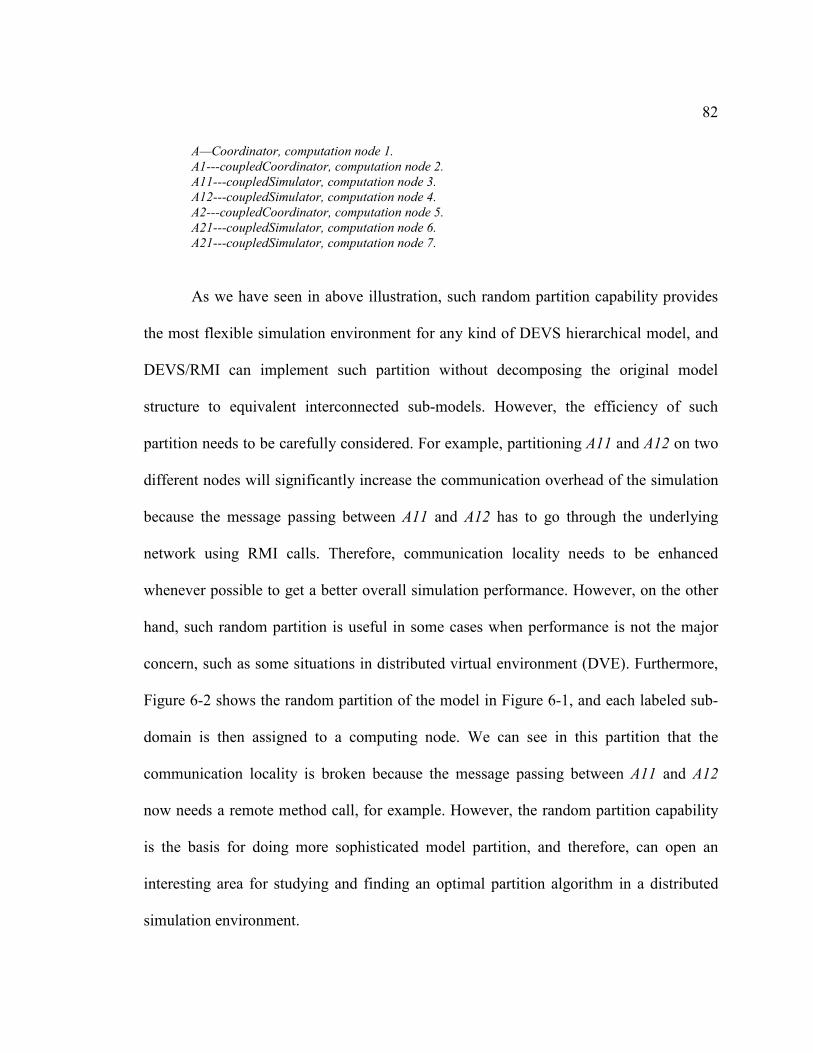
82
A—Coordinator, computation node 1.
A1---coupledCoordinator, computation node 2.
A11---coupledSimulator, computation node 3.
A12---coupledSimulator, computation node 4.
A2---coupledCoordinator, computation node 5.
A21---coupledSimulator, computation node 6.
A21---coupledSimulator, computation node 7.
As we have seen in above illustration, such random partition capability provides
the most flexible simulation environment for any kind of DEVS hierarchical model, and
DEVS/RMI can implement such partition without decomposing the original model
structure to equivalent interconnected sub-models. However, the efficiency of such
partition needs to be carefully considered. For example, partitioning A11 and A12 on two
different nodes will significantly increase the communication overhead of the simulation
because the message passing between A11 and A12 has to go through the underlying
network using RMI calls. Therefore, communication locality needs to be enhanced
whenever possible to get a better overall simulation performance. However, on the other
hand, such random partition is useful in some cases when performance is not the major
concern, such as some situations in distributed virtual environment (DVE). Furthermore,
Figure 6-2 shows the random partition of the model in Figure 6-1, and each labeled sub-
domain is then assigned to a computing node. We can see in this partition that the
communication locality is broken because the message passing between A11 and A12
now needs a remote method call, for example. However, the random partition capability
is the basis for doing more sophisticated model partition, and therefore, can open an
interesting area for studying and finding an optimal partition algorithm in a distributed
simulation environment.

83
Figure 6-2A Random Partition Showing the Assignments of Atomic Models to
Computing Nodes
Compared with random model partition, re-grouping the models to sub-domains
while considering communication locality is another important partitioning technique
implemented in DEVS/RMI. This technique is especially useful to handle large-scale
cell-space models. In such model, the depth of model hierarchical tree is relative small,
and the focus of the partition is generally on how to assign the grouped cells to the
computing nodes.
Figure 6-3 2D Cell Space
Cell 11 Cell 12 Cell 13 Cell 14
Cell 21 Cell 22 Cell 23 Cell 24
Cell 31 Cell 32 Cell 33 Cell 34
Cell 41 Cell 42 Cell 43 Cell 44
2D Cell Space
Sub-domain 1 Sub-domain 2 Sub-domain 3
A11 A12 A21 A22

84
Figure 6-4 Coupling Relationship Among Cells
Figure 6-3 shows a generic 2D cell space model (4 by 4) with coupling
relationship among cells shown in Figure 6-4, where any cell that is not on the edge of
cell space is coupled with its eight nearest neighbors. It is easy to see that for such cell
space model, randomly partitioning cells to the computing nodes is not an efficient
approach because of the tight coupling relationship among cells showed in Figure 6-4.
How to re-group cells to sub-groups/domains is especially important to obtain best
overall simulation performance.
Figure 6-5 Evenly Divided Sub-Domains of 2D Cell Space Model
Cell i-1,j-1 Cell i-1,j Cell i-1,j+1
Cell i, j-1 Cell i,j Cell i, j+1
Cell i+1,j-1 Cell i+1,j Cell i+1,j+1
Cell Cell Cell Cell
Cell Cell Cell Cell
Cell Cell Cell Cell
Cell Cell Cell Cell
Sub-Domain 1 Sub-Domain 2
Sub-Domain 3 Sub-Domain 4

85
Figure 6-5 shows the evenly divided sub-domains of the 2D cell space model in
Figure 6-3. The evenly divided sub-domains means that the number of cells in each sub-
domain are equal. Compared with random partitioning, such partition needs the re-
construction of the original model. As shown in Figure 6-5, each sub-domain now
belongs to a new digraph, and cells on the edge of the digraph needs added new coupling
to their digraph. The original coupling relationship can be maintained by further
constructing the coupling among these sub-domain digraphs.
Figure 6-6 shows a more general case, where cells in the cell-space are irregularly
divided to several different computing sub-domains, and then assigned to different
computing nodes. Any cell on the edge of sub-domain digraph needs creating coupling to
the digraph it belongs to in order to maintain the original coupling relationship. It is
worth to note that such irregular partition is useful when each individual cell cannot be
equally weighted in terms of computing workload. For example, in a certain time period,
some cells have more computing workload than other cells. In such a case, using such
irregular partition is necessary to get an overall load-balance of the computing in a
distributed environment. In some cases, if the individual cell cannot be treated with equal
or similar computing workload for a simulation run, some heuristic function should be
used to estimate the computing workload on each cell (or group of cells) before initiating
a model partition plan.

86
In general, dynamic re-partitioning technique needs to be applied to obtain best
processor’s utilizations because of the dynamic nature of some of the modeled systems.
We will discuss such technique in the following section.
Figure 6-6 Irregular Re-Group the Cells to Different Computing Sub-Domains
6.2 DYNAMIC REPARTITION
6.2.1 Overview
Dynamic model partition/repartition applies or changes the model partition plan
during simulation runtime. In dynamic model partition, the models are repartitioned on
demand, and are always dynamically migrated among the computing nodes. In such a
circumstance, the simulation loop temporarily stops by the simulation controller and then
resumes its execution after the model migrations are finished. Figure 6-7 illustrates an
example for dynamic model repartition in DEVS/RMI. The figure on top shows the initial
model partition in two sub-domains. The bottom figure shows that the “cell 13” and
Cell Cell Cell Cell
Cell Cell Cell Cell
Cell Cell Cell Cell
Cell Cell Cell Cell

87
“cell 23” in “sub-domain 2” are migrated to “sub-domain 1” during run-time. Such a
process is accomplished by decoupling the “cell 13” and “cell 23” from their neighbor
cells and sub-domain boundary (or say the digraph to which they belong), and then
migrating them by a RMI call at simulation controller such as RMICoordinator. After
such model migrations, new couplings need to be added to maintain the overall coupling
relationship among cells in the cell-space. As we have mentioned before, such dynamic
decoupling and re-coupling (or adding new couplings) can be done by using “Variable
Structure” technique in DEVS/JAVA and DEVS/RMI. It is also worth to mention that
dynamic repartition is called on when load-balance of the distributed simulation is a
major concern for the tested model. In general, dynamic repartition is helpful for gaining
optimal processor utilizations, and therefore, may enhance the performance of distributed
simulation.

88
Figure 6-7 Dynamic Model Repartition in DEVS/RMI
6.2.2 A Dynamic Repartition Example
We will now exemplify the dynamic model repartition using a DEVS “gp” model,
which consists of a “generator” and multiple “processors”. As shown in Figure 6-8, a
“generator” with multiple “processors” (total number is n, a variable to represent number
of “processors” involved in test) is assigned to machine 1, and an individual “processor2”
is assigned to machine 2 by DEVS/RMI simulation controller—RMICoordinator. The
distributed simulation initializes and starts with this setting and then temporally stops
Bold lines represent newly added coupling
Cell 11 Cell 12 Cell 13 Cell 14
Cell 21 Cell 22 Cell 23 Cell 24
Sub-Domain 1 Sub-Domain 2
Coupling
Cell 11 Cell 12 Cell 13 Cell 14
Cell 21 Cell 22 Cell 23 Cell 24
Sub-Domain 1 Sub-Domain 2
Coupling
These arrow lines represent the coupling that will be
removed.
Migration
Migration

89
during run-time. The RMICoordinator then dynamically migrates the n processors (from
“Processor10” to “Processor1n”) from machine 1 to machine 2, and re-constructs the
couplings among the “generator” and “processors”. Figure 6-9 shows the re-constructed
model structure and the updated models’ physical locations. After this model dynamic
migrations with persistent states, the simulation continues its execution.
Figure 6-8 A DEVS “gp” Model Before Model Repartition
Figure 6-9 A DEVS “gp” Model After Model Repartition
Generator
Processor10
Processor11
Processor1n
Processor2
………….
Machine 1 Machine 2
Generator
Processor10
Processor11
Processor1n
Processor2
………….
Machine 1 Machine 2

90
Figure 6-10 and Figure 6-11 are dump screens showing the dynamic repartition in
actions using SSH tunneling to access remote USGS Beowulf cluster. The output of this
distributed execution is compared with the single machine’s execution, and the
correctness of the dynamic repartition is therefore verified.
Figure 6-10 Dynamic Repartition in Action at USGS Beowulf Cluster-1

91
Figure 6-11 Dynamic Repartition in Action at USGS Beowulf Cluster-2
Now, we look into the detail on how the dynamic repartition happens. As shown
in Figure 6-12: TestSever1 and TestSever2 on two remote machines create and register
their sub-models before RMICoordinator creates two remote references pointing to them.
The object instances of sub-models and their simulators actually exist in the two remote
machines respectively. Thereafter, the RMICoordinator initiates itself using some pre-
defined procedures, and then starts the simulation execution for certain steps. The
simulation is then temporarily stopped before the RMICoordinator calls migration
method, which actually attempts to migrate a bundle of “processors” (from number 1 to
number n) from machine 1 to machine 2. After the model migration is done, the
controller reconstructs the coupling relations to make the overall model structure
unchanged except for their actual physical location. An integer variable numberofP is

92
defined to represent the number of “processors” being migrated, which helps to
determine the overhead associated with such dynamic model migration as well as number
of migrated models. The distributed simulation is then continued from its stopping point.
Figure 6-12 Sequence Diagram for Dynamic Model Migration
As we know, the performance is a key concern for using dynamic repartition
during simulation run-time. We show some performance test result here to clarify the
overhead incurred by dynamic repartition. Table 6-1 shows how overhead incurred from
model migration is related to the number of models being transmitted across network.
Figure 6-13 demonstrates such a relation visibly using a line chart. We can see from this

93
plot that the overhead is nearly linear increased with the increased number of migrated
models. The overhead is significant when migrating large number of model components
dynamically. However, if an optimal dynamic repartition mechanism is used, the overall
distributed simulation performance is expected to be better than using static model
partition.
Number of
“p”
1 5 10 15 20 40 80 160
Overhead(s) 0.086 0.17 0.269 0.35 0.419 0.841 1.73 4.871
Table 6-1 Overhead Incurred by Dynamic Model Migration
Overhead vs. No. of Migrated Models
0
1
2
3
4
5
6
0 20 40 60 80 100 120 140 160 180
Number of Migrated Models
Overhead(seconds)
Overhead vs. No. of Migrated Models
Figure 6-13 Overhead Incurred by Dynamic Model Repartitions
The above example is presented as generic mechanism for model dynamic
migrations during simulation run-time. Due to its intrinsic flexibility, it is easy to
implement complex repartition algorithms into the simulation controller, and therefore, to
achieve higher level of dynamic load-balance in a distributed simulation environment.
94
The overhead incurred by dynamic model repartition should be carefully considered
when applying repartition algorithms. The example presented in this section could be
used as a basis for exploiting more complex dynamic model repartition techniques in a
distribute simulation environment.

95
7 INVESTIGATING THE COMPUTATION SPACE OF A SIMULATION
WITH DEVS/RMI
7.1 INTRODUCTION
In previous sections, we discussed the DEVS/RMI system architecture,
components and key functionalities, and we show our particular interests on base
performance test, dynamic reconfiguration capabilities of a DEVS/RMI system. In this
section, we will further our discussion of its application on large-scale continuous spatial
model, and we will show the advantages of using DEVS/RMI to investigate the
computation space of a simulation.
As we know, modeling and simulation has become a fundamental technique to the
modern science and engineering, and it is essentially important in predicting the future
behavior of complex dynamic systems. With the development of high performance
computing and simulation, modeling and simulation techniques are being applied in
solving very complex and large-scale problems such as those described by continuous
spatial models. Due to the limitations of a single machine’s computing power and
memory capability, parallel-distributed simulation has to be considered to solve these
continuous spatial models which in general have very large problem sizes. However, such
efforts have been proven to be a great challenge because most of mature parallel-
distributed simulation frameworks, including commercial ones, cannot handle the
distributed simulation in a transparent way.

96
Parallel-Distributed simulations of continuous spatial models typically must
address questions such as: how fine a resolution (therefore, how many cells) is needed
for acceptable accuracy? and how many computational nodes are needed for acceptable
execution time? In many applied simulations, these questions are not readily answered
because of the effort required to refactor the simulations to accommodate both increases
in cells and computation nodes. To answer such questions requires a flexible
infrastructure in which it is easy to change resolution of the model as well as partitions of
the model to the variable numbers of nodes. In this section, we show how DEVS/RMI, an
implementation of distributed DEVS using remote method invocation (RMI), provides
the flexible infrastructure required for investigating the computation space of simulation.
DEVS/RMI is used to simulate a large-scale 2D continuous cell space model, and the
experiment results show that DEVS/RMI provides a scalable simulation environment
where a large-scale cell space model can gain significant speedup when a cluster of
machines is used. The experimental results also imply that larger cell space model with a
significant computing workload could benefit from distributed simulation with
DEVS/RMI. The flexibility of DEVS/RMI opens up further investigations into the
relationship between speedup of simulation and the partition algorithm as well as the
study of techniques such as load-balancing and self-configuration during simulation run-
time.

97
7.2 SIMULATIONS OF CONTINUOUS SPATIAL MODELS
Continuous time simulation is used when the state changes occur continuously
across time within the modeled system, and such system behavior typically is described
by differential equations. In contrast, discrete event simulation is generally performed by
using computer models for a system where changes in the state of the system occur at
discrete points in simulation time [69]. Therefore, it is necessary to have a general
methodology that could combine the two into one unified framework because a lot of
systems have shown behaviors of both continuous time and discrete event. Such
combined simulation methodology was first proposed by Fahrland [70], and the need for
such combined simulations has also been addressed by Cellier [71] and Dessouky [72].
With regard to DEVS approach to such unified methodology, a formalism called
DEV&DESS subsumes both the DESS(for continuous system) and the DEVS (for
discrete event system), and thus supports the development of coupled systems whose
components are expressed in any of the basic formalisms [1]. Such multiformalism
modeling capability is very important to handle real-world simulation since some of the
modeled system behavior has to be captured by using both DESS and DEVS. As an
example, a chemical plant is usually modeled with differential equations while its control
logic is best designed with discrete event formalism [1].
DEVS approach to continuous state systems, such as those described by
continuous spatial models, uses quantized state system to integrate the DEVS with the
DESS. A quantized system is a system with input and output quantizers [73], and it uses
quantization to generate state updates but only at quantum level crossings, which affords

98
an alternative, efficient approach to embedding continuous models within discrete event
simulations. DEV/DESS has provided a framework to represent classes of continuous
and discrete systems, and makes it possible to develop object-oriented simulation
applications with such models.
Continuous spatial models are those models in which two or three dimensions are
represented [74], and they could be solved by the combined simulation techniques such
as DEV/DESS. In order to get the acceptable accuracy of the simulation of such spatial
models, resolution needs to be increased by adjusting the computation space of the
model. However, the increased resolution commonly needs larger cell space size to be
simulated, and therefore, requires more computation power in the computation space of
the simulation. With the demand for obtaining higher resolution of such models, the
computation space has to be increased accordingly until all the resources for a single
machine are used up. In such a case, parallel-distributed simulation is most likely to be
called on to get the desired resolution by distributing the computation space to sub-
spaces, and then mapping to a cluster of machines. However, a flexible simulation
framework is necessary to deal with such model scale changes as well as the feasibility of
mapping the model to computation nodes.
7.3 HILLY TERRAIN MODEL
In this section, we focus our discussion on a hilly terrain model, which is a two
dimensional continuous spatial cell space model to simulate how a traveler finds the
smallest travel time to a goal point taking account of hilliness of the terrain. The smallest

99
travel time is measured by the simulation as a function of number and placement of
“hills” where “hills” combine to provide a gradient to each point in a 2D space. The time
to traverse a small region is related to the gradient in the following way: if the gradient is
positive in the traveler’s direction, then the travel time is directly related to its magnitude
(going up slows progress); if the gradient is negative, then the travel time is inversely
related to its magnitude (going down increases progress).
Adding hills in the 2D space increases the computing workload required for each
individual cell in the model. The larger the workload on each cell, the greater the benefit
to be expected from distributed simulation. It is also worth to note that increasing number
of cells results in the increase of memory usage and computational workload for the
simulation engine. As shown in Figure 7-3, each terrain cell represents a DEVS atomic
model with possible states: “output”, “firstoutput”, “secondoutput”, “refractive”,
“receptive”, and etc. Each terrain cell has its own X-Y coordinates in the space and has
eight input and eight output ports for coupling with its existing nearest neighbors. For
example, the cells residing in the inner 2D space are coupled with 8 nearest neighbors,
while the cells residing on the edge or corner of the space are coupled with less than 8
neighbors. Consequently, each cell is influenced by any of its nearest neighbors through
these couplings.
Figure 7-1 shows how to calculate the gradient and the time to traverse a distance q
for a 1D hilly terrain model. A hill in the space is modeled and represented by the
function h(x), where H represents the height of the hill and c is the central location of the
hill. The time to traverse a distance q (represented by a quantum in DEVS) is a function

100
of q and the gradient of the hill at a given location x. If the gradient is positive, the time to
traverse q increases; if the gradient is negative, the time to traverse q decreases.
Figure 7-1 Calculate Hilliness and Traversed Time in 1D Space
Moreover, Figure 7-2 shows how to calculate the hilliness in a 2D hilly terrain
space as used in this section, where (ci,cj) represents the x-y coordinator of the center of a
hill in the space, and H(ci,cj) is the height of this hill. The hilliness of the 2D cell space
can then be obtained by sum of the h(ci,cj) (x,y) functions for all hills. The hilliness is used
to calculate the gradient at certain location (x,y), and is then applied to determine the
direction of the traveler at any point in the space. In order to get the shortest travel time
from point A to B, at certain point (x,y), the traveler goes to the “north” or “east”
according to the smaller steepness of the hill between x and y direction, by calculating the
gradient at point (x,y)---partial derivatives of h(x,y) to x and to y.

101
Figure 7-2 Calculate Hilliness in 2D Space
The continuous spatial hilly terrain model, described by the mathematic functions
in Figure 7-1 and Figure 7-2, is then modeled in DEVS using quantization technique. The
resulted DEVS model can then be simulated in DEVS/JAVA and DEVS/RMI for
studying the computation space of it. In the following sections, we will present the
detailed implementation, and we show particular interests on the speedup of the
simulation when running this model in a distributed environment provided by
DEVS/RMI.

102
Figure 7-3Hilly Terrain Model in Simview
7.4 WHY DEVS/RMI FOR HILLY TERRAIN MODEL
Hilly terrain model was initially constructed and simulated in DEVS/JAVA in a
single machine. However, due to the limitations of a single machine’s CPU power and
memory capability, the cell-space size cannot exceed 100 by 100, at which point the out
of memory error of Java VM appears. It is wise to consider increasing the memory for
Java runtime, and an interesting finding is that the Java VM provides only 64M heap
memories as default for regular applications, which is apparently not sufficient enough
for a large cell space model. With such a consideration, a Java runtime parameter “-
Xmx1024m” was used to increase the Java runtime memory at the maximum value for a
regular desktop PC, which generally has a 256M, 512M or 1024M memory. It did solve

103
the problem a little further and some model cases with a size of 150 by 150 can run,
although considerable amount of time is necessary to get the result. However, a cell space
larger than 150 by 150 cannot be solved in any means in the tested single machine with
512M physical memories. In order to make this situation clearer, let’s do a simple Math
for memory estimation. For example, to initialize a 150 by 150 cell space model, 2 by
150 by 150 DEVS/JAVA model and simulator objects are necessary, and each of these
300 by 150 objects also create other relevant objects. If each model/simulator object
creates 10 related objects and we assume the average occupied memory for each object is
1000 bytes, the total necessary memory is around 450M. Although the heap memory
occupied by Java objects is garbage collected, cell objects cannot benefit from this
dynamic memory management because they are statically created before a simulation
execution starts. It is worth investigating how such a limited memory problem could be
solved by distributed simulation, such as using DEVS/RMI.
Another major reason to use DEVS/RMI to simulate the hilly terrain model is that
such a simulation needs a flexible and scalable distributed framework to reach the
model’s necessary resolution when the problem size goes out of capability for a single
processor’ CPU and memory capabilities. For example, it is not easy to re-tailor and
revalidate the model when a middleware solution is applied, which generally adds
additional simulator control layer and time management layer. As presented in previous
sections, DEVS/RMI can provide a flexible and scalable infrastructure, which can be
easily applied to refactor the simulation application in a circumstance when both problem
sizes and computation nodes need increase. In the following experimentation,
104
DEVS/RMI works by changing computation space of a simulation at model initialization
phases, and maintains the same partition algorithm for the increases of the both cell space
size and the computing nodes. This is due to the seamless support for distributed
simulation of DEVS/RMI, which does not rely on additional layers on top of its
simulation engine. By using easily configured simulation experiments of DEVS/RMI, it
is easy to answer questions such as how fine a resolution (therefore, how many cells) is
needed for acceptable accuracy? And how many computational nodes are needed for
acceptable execution time? In contrast, in many other approaches, such questions are
difficult to be answered.
7.5 LINUX CLUSTER
In this experiment, 3, 6 and 11 nodes of a 40 nodes Linux cluster are used to test
the hilly terrain model under DEVS/RMI. Each node in the cluster has an AMD Athlon
XP 2400+ with 2GHz CPU and 512M physical memories, and all the nodes are
connected by 100M Ethernet switch with TCP/IP as communication protocol. The
operating system of each node is GNU/Linux 2.4.20 with Java Runtime 1.4.1-01
installed.
7.6 MODEL PARTITION FOR HILLY TERRAIN MODEL
In order to run the hilly terrain model in DEVS/RMI in an efficient way, the
original model is partitioned to computing nodes by dividing it into several
interconnected sub-models. In this experiment, the hilly terrain model is evenly divided

105
by columns according to the number of computing nodes used for testing. As shown in
Figure 7-3 and Figure 7-4, the digraph of original cell space is divided into two sub-
digraphs, which are interconnected to each other through input/output ports. In fact, the
inter-connected sub-digraphs are equivalent to the original digraph in terms of coupling
relations of cells in the space. Thereafter, each sub-space can be assigned to a computing
node easily. It is verified that the partitioned model has the same output result when
running in DEVS/RMI compared with the original model running in a single machine
using DEVSJAVA. The reason to do such a partition is that sub-digraphs could be
assigned to computing nodes evenly and then be controlled by their local
RMICoupledCoordinators, and thus avoid RMI calls within sub-digraphs. This model
partition mechanism has been proposed and discussed in earlier chapters aiming to
increase the locality. Each subspace, for example, “s0” or “s1” in Figure 7-4 is assigned
to different computing nodes respectively and either of them is controlled locally by the
corresponding RMICoupledCoordinator, which is then controlled by RMICoordinator
residing on the main simulation control node.
In general, such model partition aims to reduce the RMI overhead caused by
message passing among cells. Although such partition involves generating a new
equivalent model of original model, the overall message passing efficiency may be
increased due to reduced RMI overhead.

106
Figure 7-4 Divided Hilly Terrain Model in Simview
7.7 AUTOMATIC TEST SETUP
For a large-scale model such as hilly terrain model, it is necessary to set up the test
using DEVS/RMI in an automatic way in order to make collecting experimental data
more efficient. Therefore, on each computing node, the same RMI server program is
started for accepting the request from the simulation main control node. The main
program in simulation main control node actually uses synchronized threads to initialize
all the computing nodes at first. Each thread generally uses a RMI call to let the
corresponding computing nodes to start creating and registering its models as well as
simulators/coordinators. When this initialization phase finished on all computing nodes,
the main control program then automatically continues executing and starting the
simulation control loop. This automatic setup is very important for simulating large-scale

107
cell space because it is not practical to manually start the initialization phase in each
computing node, and then to wait for their finishing after a long time delay.
As shown in Figure 7-5, RMICoordinator calls the regSimulator() method to
initialize the creation and registration of remote simulators on two remote machines,
which host TestServer1 and TestServer2. After this procedure is finished, the
RMICoordinator then starts the simulation execution loops. Therefore, the overall
distributed simulation is fully automatically initialized and controlled by the “head” node
running RMICoordinator.
Figure 7-5 Sequence Diagram for Automatic Setup Distributed Simulation

108
7.8 SPEEDUP OF SIMULATION FOR HILLY TERRAIN MODEL
In this section, some experiment results for the distributed simulation of hilly
terrain model are presented and discussed. The focus is on the performance of the
DEVS/RMI when being applied on a cluster of computing nodes to solve large problem
sizes for this model.
As aforementioned, the purpose of simulating hilly terrain model is to obtain the
shortest travel time of a traveler in a terrain. As added obstacles for the traveler, the
existence of hills in the terrain delays the shortest travel time. The size of the cell space
determines the resolution of the measurement of the shortest travel time, however,
oversized cell space is not necessary to capture the converged shortest travel time
constant for a given condition of hills in the space. Figure 7-6 shows how the simulation
resolution for the hilly terrain model relates to the number of cells (or say problem size).
When the number of cells reaches certain level, the measured travel time converges to a
constant. This constant is different for different number of hills as well as the setting of
these hills in the cell space because the hills in the cell space directly affect the shortest
travel time. Figure 7-7 shows how the travel time increases with number of hills in the
cell space. With the increase of the hills in the space, the number of cells in the space
needs to be increased significantly in order to find the converged constant. Therefore, a
scalable simulation framework such as DEVS/RMI is on demand to solve this simulation
problem.

109
Travel Time vs. No. of Cells
0
100
200
300
400
500
600
700
800
900
1000
0 10000 20000 30000 40000 50000
Number of Cells
Travel TIme
one hill
four hills
Figure 7-6 Travel Time vs. Number of Cells
Travel Time vs. No. of Hills
0
2000
4000
6000
8000
10000
12000
14000
0 5 10 15 20 25
Number of Hills
Travel Time
100 by 100 cell space
Figure 7-7 Travel Time vs. Number of Hills
In fact, DEVS/RMI works straightforwardly on obtaining the shortest travel time
constant for a cell space with added hills by scaling the model to larger sizes. A cell space

110
with one hill is also tested to compare with the model with 100 hills in the cell space.
Increasing both the cell space size and the computing nodes is easily accomplished using
DEVS/RMI, and does not alter the model domain-decomposition technique used in this
experiment. Figure 7-8 shows the speedup for simulation initialization time by
DEVS/RMI using 3, 6 and 11 nodes for one hill and 100 hills respectively in the cell
space. It could be seen that the initialization speedups increase dramatically with the
increased computing nodes for a fixed cell space size, because each node initializes only
one partitioned sub-space. However there is almost no difference of speedup for one hill
and 100 hills, for a given number of nodes, because adding hills has no effect to cell
space size and the speedup of initialization is only related to the number of cells on each
computing node. It is easy to find that adding computing nodes can greatly reduce the
initialization time for the simulation, especially for larger cell space model.
Speedup of Initialization Time
0
10
20
30
40
50
60
70
80
0 5000 10000 15000 20000 25000
No. of Cells
Speedup(single/multi-nodes)
1 hill 3 nodes
1 hill 6 nodes
1 hill 11 nodes
100 hills 3 nodes
100 hills 6 nodes
100 hills 11 nodes
Figure 7-8 Speedup of Initialization Time with DEVS/RMI

111
Speedup of Simulation
0
0.5
1
1.5
2
2.5
3
3.5
4
0 2500 5000 7500 1000
0
1250
0
1500
0
1750
0
2000
0
2250
0
2500
0
No. of Cells
Speedup(single/multi-nodes)
3 nodes one hill
6 nodes one hill
11 nodes one hill
3 nodes 100 hills
6 nodes 100 hills
11 nodes 100 hills
Figure 7-9 Speedup of Simulation Using DEVS/RMI
Figure 7-9 shows the speedup of the simulation by DEVS/RMI using 3, 6 and 11
nodes for one hill and 100 hills in the cell space. For one hill, the speedup of the
simulation execution time increases from below 1 to near 1 when increasing the number
of cells in cell space, and adding more nodes actually degrade the performance. This is
because adding one hill in the hilly terrain does not increase enough workload on each
cell to compensate the increased communication workload incurred by RMI calls.
When 100 hills are added to the cell space, each cell is injected with a significant
workload and the overall workload for the cell space increases with the increased number
of cells. However, for a fixed cell space, with the increased computing nodes, each node
has less computing workload but with increased communication workload due to the
RMI calls among the edge cells on each node as well as the RMI calls between
computing node and simulation control node. Figure 7-9 shows that for a 100 by 100 cell

112
space, a maximum speedup could be achieved by using 11 nodes. When cell space size
continuously increases beyond 100 by 100, the speedup decreases for all 3, 6 and 11
nodes for 100 hills due to the increased RMI calls incurred by increased edge cells. In
general, for a larger cell space in this experiment, increasing computing nodes also
increases speedup of simulation if each cell has enough workload on it. This experiment
implies that there is an optimal point for speedup when both problem size and computing
nodes increase. DEVS/RMI makes it easy to locate such critical points by scaling the
simulation transparently from single processor to multiple processors.
7.9 SIMULATING VERY LARGE HILLY TERRAIN MODEL
A 400 by 400 hilly terrain model is tested under DEVS/RMI with 8 computational
nodes, and it works with no problem but needs considerable amount of time to get the
result because the necessary simulation loops increase significantly with the increase of
the cell space size for this particular model. However, this verifies that DEVS/RMI could
solve very large cell-space models as long as the necessary computing nodes are
available with the help of distributed memory technology used in DEVS/RMI.
7.10 CONCLUSION
We have seen in this chapter that DEVS/RMI provides a very flexible, dynamic
and scalable distributed simulation infrastructure, which could be easily applied to
refactor the simulation applications in a circumstance when both problem sizes and
computation nodes need increase. The experimental results could directly help on

113
answering the questions such as: how fine a resolution (therefore, how many cells) is
needed for acceptable accuracy? and how many computational nodes are needed for
acceptable execution time? This is because that refactoring the spatial model in the
experiment is transparent with the help of DEVS/RMI.

114
8 LARGE-SCALE DISTRIBUTED AGENT BASED SIMULATION USING
DEVS/RMI
8.1 DISTRIBUTED SIMULATION OF VALLEY FEVER MODEL
In this chapter, we further our discussion on DEVS/RMI by investigating a highly
dynamic 2D cell space model called valley fever. We focus our discussion on how
speedup of the distributed simulation relates to the partitioned workload on the
computing nodes, and we will continue our interests on examining the concept of model
“activity” and how it affects the workload distribution in a distributed simulation
environment.
8.1.1 Valley Fever Model
The Agent-based Valley Fever Model initially designed by Bultman, Fisher and
Gettings [66] is a 2D dynamic cell space model to represent how the fungal spores grow
on a patch of field over a long period of time with given environmental conditions such
as wind, rain, moisture and etc. As shown on Figure 8-1, it consists of several individual
model components: wind model, rainfall model, coupling control model and patch model.
All these components are DEVS atomic models except patch model, a DEVS coupled
model consisting of an atomic model called “Sporing Process” and another atomic model
called “environment”. All these models are assigned to a 2D cell space DEVS diagraph
and the patch models are in fact have X-Y coordinator in the cell space. The wind model
and the rainfall model are both statistic models which can generate wind data and rain
data periodically. The output from them are then sent to the coupling control model
which uses the input rain data and wind data to determine the dynamic coupling of rain

115
model with patches as well as the dynamic coupling among patches. This model structure
is highly dynamic and changes its structure on each simulation step.
Figure 8-1Valley Fever Model in DEVSJAVA SimView
8.1.2 Model Partition for Valley Fever Model
In this experiment, the static model partition is used in order to reduce the cost of
dynamically creating remote simulators with models passing as parameters. Several
different partition methods are tested and it was found that the distributing other model
components except patch cells does not have much difference regarding the simulation
execution time. With the increase of the patch cells for the model, it is easier to see that it
is necessary to partition these cells.

116
Therefore, the patch cell space is evenly divided by columns according to the
number of computing nodes. For example, to partition a 10 by 10 patch space on 5 nodes,
every two columns of cells is assigned to one node. All the other model components are
sitting with the simulation control node. On each computing node, a program called
“testserver” is started to start RMI registry by itself and creates a set of simulator/model
pairs which belong to this node according to the model’s putWhere() attributes, then the
references of the simulators are registered with RMI registry for the lookup by the
RMICoordinator. After above mentioned initialization of each node, the RMICoordinator
is started at the main simulation control node.
8.1.3 Distributed Simulation Results for Valley Fever Model
As shown in Figure 8-2, a 10 by 10 patch space is divided into 1, 2, 5, 10 nodes
respectively to measure the total simulation execution time in terms of 100 simulation
loops. It can be seen that the simulation time has a significant increase with the increase
of the computing nodes due to the added communication overhead, however, there is no
significant execution time increase for simulating the model among two nodes, five nodes
and ten nodes.

117
0
100
200
300
400
500
1 2 5 10
Execution
Time(S)
Figure 8-2 Simulation Execution Time(seconds) vs. No. of Computing Nodes in
Original Model
8.1.4 Workload Injection to the Distributed Cells
From the experiment result obtained from above section, it can be inferred that the
increase of simulation execution time is due to the increased communication workload
among the nodes. It is worthwhile to examine what may happen if the workload is
increased on distributed cells without increasing the communication workload (such as
number of RMI calls through network). A 5 by 5 cell space is tested in terms of 400
simulation loop in order to get the experiment result relatively quicker. Figure 8-3 shows
how the situation changes compared with the result obtained in original model when
different workload is injected to the distributed cells. For the figure on left side, whenever
each patch cell gets an external event, it calculates the sum of integers from 1 to 100 as a
way to add computing workload. It can be seen that the total execution time of overall
simulation is slightly increased for 5 nodes compared with for 1 node. For the figure on
the right side, whenever each patch cell gets an external event, it calculates the sum of
integers from 1 to 150, and we can see that the total execution time of overall simulation

118
is greatly reduced when using 5 nodes compared with using only 1 node. It can be then
seen that the workload on the distributed cells plays an important role in affecting the
performance of the distributed simulation. This experiment result implies that, for the
original valley fever model, the distributed cells do not have enough workload to
compensate the cost of increased communication incurred by RMI calls across network.
0
200
400
600
800
1000
1 5
workload1
0
1000
2000
3000
4000
5000
6000
7000
8000
1 5
workload2
Figure 8-3 Simulation Execution Time(seconds) vs. No. of Computing nodes
Under Different Workload on Distributed Cells
From all of above experimentations, we have seen that DEVS/RMI plays an
important role in solving large-scale cell DEVS models in a transparent and scalable
fashion. The experimental results imply that a larger cell space model with a significant
computing workload can benefit from distributed simulation with DEVS/RMI in terms of
getting positive speedup.

119
8.2 DYNAMIC RECONFIGURATION OF DISTRIBUTED SIMULATION OF
VALLEY FEVER MODEL USING ‘ACTIVITY’
8.2.1 Introduction
From our previous discussions, we could say that it is worth investigating model
partition algorithms, in particular, dynamic partition or repartition techniques in order to
improve the performance of distributed simulation. Dynamic partition or re-partition is
important for complex simulation models, where their run-time behaviors are difficult to
predict. However, a well-defined model partition plan is hard to obtain in practice when
running the model in distributed fashion. Therefore, a parallel or distributed simulation
framework that supports dynamic reconfiguration is needed to properly study dynamic
repartitioning of simulation models on clusters of machines.
In the previous section, we use a static “blind” model partition for running valley
fever model in DEVS/RMI in a distributed fashion. We have found that the workload in
the partitioned cells plays an important role in affecting the distributed simulation
performance. In this section, we will focus on dynamic reconfiguration in distributed
simulation, and particularly, we are interested in how “activity” affects the model
partition and consequently influences the performance of distributed simulation. We
exemplified such a concept of “activity” by continually using the valley fever model
discussed in previous section.
As presented in some earlier work [67][68], DEVS based distributed simulation
framework uses “activity” as a measure of computing workload. As we know, DEVS
provides a solid simulation methodology for representing asynchronous spatial behavior

120
that is usually implemented by time-stepped simulation. Therefore, in this section, we
show how to exploit the heterogeneity of model behavior in time and space that often
results from such DEVS representations. And then we use such “activity” metric to
balance the computation workload using dynamic reconfiguration of distributed
simulation. We will show how to exploit this “activity” metric to improve the distributed
simulation performance by using an activity-based partitioning approach.
In the following sections, we present a dynamic reconfiguration mechanism that
uses an “activity” metric which is dynamically gathered before a distributed simulation
execution, and therefore, provides a useful information for deciding an improved model
partition plan. Consequently, such a partition plan will prove to be better than a blind-
partition in terms of simulation execution performance.
8.2.2 Static Blind Model Partition vs. Dynamic Reconfiguration Using “Activity”
In order to compare with the dynamic model partition using “activity”, static blind
model partition is used to map the “patches” models to computing nodes. In this setting,
“wind”, “rain” and “coupling_control” models are all arranged at the “head” node, and
the “patches” cells are evenly divided to other computing nodes in a “blind” fashion, i.e.,
without regard to their measured activities. For example, for a 4 by 4 cell space to run on
4 computing nodes, each column of cells is assigned to one computing node resulting in
an evenly distributed cells to computing nodes-- 4 cells on each node.
The static blind model partition does not consider the imbalance of workload on
each individual cell. Some cells may have less “activity” than others, and therefore, are

121
subject to less computing workload. To partition the cells blindly results in imbalance of
workload of computing nodes, which cannot benefit the overall simulation performance.
In general, for a given highly dynamic simulation model such as valley fever, it is
difficult to predict the model run-time behavior.
Fortunately, in the valley fever model, production of spores is the main driver of
activity in patches. “Sporing” is largely determined by the strength and direction of the
wind which is an external input to the model. New “sporing” patches are typically highly
concentrated in the direction of the wind. The fact that wind regimes change relatively
infrequently allows us to obtain stable activity distributions using simulation on a single
machine for each such regime. Activity at each cell is measured over such a period as the
total number of internal transitions that the cell undergoes during that period.
Experimentally, we verify that this number is closely related to the computational
intensity required to simulate a cell during such a period.
Given the dependence of activity on wind regimes, we can measure model
“activity” by executing the model (on a single machine or in distributed fashion) for
desired wind regimes and gather the model “activity” metric through such a run. This
information can then be applied to obtain a model partition plan for a distributed run of
the same model configuration. Since the wind regime is controlled externally to the
model, we can monitor the wind generator and apply the partition plan that is optimal for
a regime whenever the wind changes. We measure the model activity through counting
the internal transitions of the ‘sporingProcess’ to see how a dynamic model partition
using such information can benefit the distributed simulation performance. In this

122
example, a simplified method is used to determine a subset of cells called high-activity
cells. Firstly, the average internal transition count of all the cells in the cell space is
obtained by running the model in the head node for a given wind regime. At the end of
this run, each cell compares its own count with the average, if it is larger than the
average, the cell’s id is added to a linked list data structure for high-activity cells. Figure
8-4 illustrates how high-activity cells are selected from the cell space.
Figure 8-4 Selecting High-Activity Cells
After the high-activity sets are obtained for each wind regime, the following
process occurs within a single simulation run. The RMICoordinator in the head node
creates a new valley fever model and partitions it according to the initial wind regime.
Every time a new wind regime is detected, the RMICoordinator creates a new valley
All Cells
Counting number of
internal transitions
of each cell
Calculate Average of
internal transitions
Add this cell to
high-activity list
If this cell’s number of internal transitions is larger than the
average Else
Add this cell to
low-activity list
Compare each cell with
average

123
fever model, and partitions its cells so that the high activity cells for that regime are
granted more computing power than are the remaining cells. Finally, the cells are
dynamically loaded to computing nodes and the distributed simulation is then re-started
from the state that the model was in before the repartition.
In the following test, we discuss one iteration of this process in which all the low
activity cells are assigned to one computing node, and all the high activity cells are then
evenly distributed to other available computing nodes. Some test results are presented in
next section.
8.2.3 Test Environment and Results
In this experiment, 5 nodes of a 40 node Linux cluster are used, where each node
in the cluster has a AMD Athlon XP 2400+ with 2GHz CPU and 512M physical
memory. All the computing nodes are inter-connected by 100M Ethernet switches, and
the operating system of each node is GNU/Linux 2.4.20 with Java Runtime 1.4.1-01
installed.
In this test, static blind partition is compared with dynamic reconfiguration in
terms of simulation execution time. A 4 by 4 and 8 by 8 cell spaces are used and are
executed with 400 and 2000 simulation steps. The purpose of this test is to verify the
advantage of using “activity” based dynamic repartition when compared with static
“blind” model partition. Such verification will also prove that the model “activity” is a
more accurate indicator for computing workload for the examined cells in a cell space.

124
Using 5 computing
nodes including 1 head
node.
Static Blind Partition not
considering model
activities
Dynamic
reconfiguration
using “activity”
Performance
increase by
percentage
4 by 4 cells with 400
simulation steps
28.124s 27.566s 1.98%
4 by 4 cells with 2000
simulation steps
113.977s 114.968s -0.87%
8 by 8 cells with 400
simulation steps
256.49s 248.644s 3.06%
8 by 8 cells with 2000
simulation steps
1238.479s 1216.97s 1.73%
Table 8-1 Distributed Simulation Execution Time for Static Blind Partition and
Dynamic Reconfiguration Using “Activity”—5 nodes.
Using 9 computing
nodes including 1 head
node.
Static Blind Partition not
considering model
activities
Dynamic
reconfiguration
using “activity”
Performance
increase by
percentage
4 by 4 cells with 2000
simulation steps
134.74s 110.49s 18%
8 by 8 cells with 2000
simulation steps
1348.17s 1199.87s 11%
Table 8-2 Distributed Simulation Execution Time for Static Blind Partition and Dynamic
Reconfiguration Using “Activity”—9 Nodes.
As shown in Table 8-1, for a 4 by 4 cell space, there is no noticeable difference
when using dynamic reconfiguration. However, for 8 by 8 cell space, dynamic partition
using model “activity” improves the simulation performance in a noticeable manner. This
is because for a 4 by 4 cell space, there is only several cells difference in each computing
node, and these cells cannot contribute too much on workload difference. It could be

125
expected that for a large cell space with long simulation execution steps, model “activity”
could play an increasingly important role on affecting distributed simulation
performance. Table 8-2 further verifies our expectation on performance improvement
when more computing nodes are used on high-activity cells. We can see a significant
performance increase using “activity” based model repartition.
The test results suggest that it worth further investigating the concept of model
“activity” in more detail and to develop model partition plans that exploit the activity
distributions in a more precise way.
8.2.4 Discussion
In this section, we present and demonstrate how DEVS “activity” affects
performance of a distributed simulation. Dynamic model reconfiguration plays a very
important role for large-scale and highly asynchronous and irregular models. We have
seen that dynamic model reconfiguration using the “activity” metric can improve
distributed simulation performance. It is also worth to note that DEVS/RMI provides a
flexible distributed simulation environment for studying and investigating dynamic
model partition/repartition algorithms.
For the future work on the “activity” based distributed simulation, adaptive
reconfiguration needs to be investigated to improve the distributed simulation
performance. The concept of “activity” needs to be studied further to provide more
detailed information on how significant changes in activity distribution can be detected
during run time as a basis for dynamic load balancing, thereby promoting an optimal and

126
dynamic reconfiguration schema for a distributed simulation execution. We have found
that high concentrations of activity in space that change relatively slowly during
simulation can be exploited to significantly reduce execution time within an appropriate
infrastructure for dynamic reconfiguration in a DEVS based distributed simulation
framework. In contrast to other dynamic load balancing approaches, the activity-based
approach discussed here exploits model properties directly rather than relying on
resource-based measurements on which to base reconfiguration.
In the next chapter, we will discuss some of the performance issues involved in
using DEVS/RMI in a distributed simulation environment.

127
9 CONCLUSION AND FUTURE WORK
From the experiments performed on the previous chapters, it is found that the
performance of DEVS/RMI highly depends on the model component partition, especially
the model component workload partition. For example, if the distributed components or
cells have less workload, the performance of the simulation can worsen compared with
that in a single machine due to the latency of the network and the remote method calls
among distributed simulators. When the workload on cells increases without increasing
the number of RMI calls, the speedup of the simulation is significant when running the
model on a computing cluster with DEVS/RMI.
Dynamic model partition/repartition in a distributed environment is fully
supported in DEVS/RMI. However, the change of model structure such as coupling
information among distributed machines is costly due to the RMI calls and network
latency. It is worth to investigate further how the dynamic model repartition could affect
the overall simulation performance in a distributed environment.
With regard to the underlying communication protocol, Sun’s RMI used in
DEVS/RMI may not be the best implementation for high performance distributed
simulation. However, a large-scale model still achieves performance advantages using
DEVS/RMI if the distributed model components have a noticeable workload. If an
alternative high-speed RMI protocol is implemented in DEVS/RMI, it can be expected
that a high performance fully object-oriented distributed simulation environment can be
built to solve very complex and large-scale simulation problem.

128
Another important issue that needs to be considered is that it is impractical to
simulate a valley fever or a hilly terrain model in a single machine with a cell space
larger than 85 by 85 because of memory limitation of a single machine. This implies that
there is a limitation of problem size when simulating large-scale cell space on single
machine, which can be solved by distributing the large size model to a computer cluster
with DEVS/RMI. In such situations, distributing the model to multiple computing nodes
is the only solution so long as the performance is not overly degraded by a
communications burden. The results for distributed simulation of a large-scale hilly
terrain model render DEVS/RMI as a promising technique to solve large-scale cell space
models that are critical for investigating some of today’s scientific and engineering
problems.
In a summary, with the increased demand for distributed simulation to support
large-scale modeling and simulation applications, much research has focused on
developing a software environment to support simulation across a heterogeneous
computing network. Among the distributed simulation frameworks, Discrete Event
System Specification (DEVS) based tools are attracting more and more attentions due to
its intrinsic properties to support object oriented modeling and simulation. Traditionally,
distributed simulations have to face the difficulties for mapping models to computing
nodes, and dynamic reconfiguration of a distributed simulation is in most cases not
possible due to the lack of the flexibilities of the implemented framework. Middleware
based solutions have been dominating for years, however, additional overhead is incurred
because of adding a new layer for simulation time management. Furthermore,

129
inconsistency exists when migrating a single machine’s simulation to multi-processor
systems, which means that a verified model has to be revalidated after it is transferred
from single processor to multi-processor. Also, model mapping is largely a manual
process which involves time-consuming work on redoing the single machine’s model
code.
In this dissertation, we have developed a new implementation of the DEVS
formalism called DEVS/RMI as a natively distributed simulation system, which aims to
reduce the overhead that is added by middleware solutions for the distributed simulation.
We have shown that DEVS/RMI has the capability to distribute simulation entities across
network nodes seamlessly without any of the commonly used middleware. Because Java
RMI supports the synchronization of local objects with remote ones, no additional
simulation time management needs to be added when distributing the simulators to
remote nodes. We have seen from our studies on the two complex and dynamic models
that such approach is well suited for complex, computationally intensive simulation
applications. It also provides an extremely flexible and efficient software development
environment for rapid development of distributed simulation applications.
We studied a hilly terrain continuous spatial in distributed simulation with support
of DEVS/RMI. In general, distributed simulations of continuous spatial models typically
must address the capability of the framework to refactor the simulations to accommodate
both increases the resolution (number of cells) and computation nodes. However, to
answer such questions requires a flexible infrastructure in which it is easy to change
resolution of the model as well as partitions of the model to the variable numbers of

130
nodes. In the experimentation of the hilly terrain model, we show how DEVS/RMI
provides the flexible infrastructure required for investigating the computation space of
the simulation. The experimental results show that DEVS/RMI provides a scalable
simulation environment where a large-scale cell space model could gain significant
speedup when a cluster of machines is used. The experimental results also imply that
larger cell space model with a significant computing workload could benefit from
distributed simulation with DEVS/RMI.
Furthermore, we show our particular interests on model partition and dynamic
repartition techniques that are implemented in DEVS/RMI. We exemplified our ideas by
investigating an agent-based valley fever model on a Beowulf cluster and found that the
speedup of the distributed simulation is directly related to the computing workload
assigned to the computing nodes. We discussed and used the concept of DEVS “activity”
concept and applied such concept on the reconfiguration of the distributed simulation.
We have seen how such “activity” can be used as a more accurate measurement of
workload distribution in a distributed simulation environment, and how “activity” based
model repartition enhances the distributed simulation performance.
We also discussed performance concerns of using DEVS/RMI and promoted
potential techniques for improving the distributed simulation performance in a
DEVS/RMI supported environment.
For the future work, it is suggested to further investigate the relationship between
speedup of simulation and the model partition/repartition algorithms. The dynamic aspect
of DEVS/RMI needs to be continuously developed and implemented to improve the

131
overall efficiency of a distributed simulation. “Activity” based model partition and
repartition need further concerns due to its role on affecting the load-balance of a
distributed simulation.

132
REFERENCES
[1]. Bernard P. Zeigler, Tag Gon Kim and Herbert Praehofer, “Theory of Modeling
and Simulation”, Academic Press, 2000.
[2]. Zhang, M., Zeigler, B.P., Hammonds, P., "DEVS/RMI-An Auto-Adaptive and
Reconfigurable Distributed Simulation Environment for Engineering Studies", ITEA
Journal, March/April 2006.
[3]. Bernard P. Zeigler, Yoonkeon Moon and etcs, "DEVS-C++: A High Performance
Modelling and Simulation Environment", Twenty-ninth Hawaii International Conference
on System Sciences, Jan. 1996.
[4]. Nutaro, J., ADEVS (A Discrete EVent System simulator), Arizona Center for
Integrative Modeling & Simulation (ACIMS), University of Arizona, Tucson, AZ,
http://www.ece.arizona.edu/~nutaro/index.php.
[5]. Wainer. G, "CD++: a toolkit to define discrete-event models", "sofware,practice
and experience",Wiley. Vol.32, No. 3, 2002.
[6]. Chungman Seo, Sunwoo Park, Byounguk Kim, and etc., “Implementation of
Distributed High-performance DEVS Simulation Framework in the Grid Computing
Environment”, 2004 High Peformance Computing Symposium.
[7]. Saehoon Cheon, Chungman Seo, Sunwoo Park, and etc., “Design and
Implementation of Distributed DEVS Simulation in a Peer to Peer Network System”,
2004 Military, Government, and Aerospace Simulation.
[8]. Jong-keun Lee, Min-Woo Lee, Sung-Do Chi, “DEVS/HLA-Based Modeling and
Simulation for Intelligent Transportation Systems”, SIMULATION, Vol. 79, No. 8, 423-
439 (2003).
[9]. Bernard P. Zeigler, Doohwan Kim, Stephen J. Buckley, “Distributed supply
chain simulation in a DEVS/CORBA execution environment”, Proceedings of the 31st
conference on winter simulation: Simulation---a bridge to the future - Volume 2,
December 1999.
[10]. B. P. Zeigler, H.S. Sarjoughian, “Approach and Techniques for Building
Component-based Simulation ModelsThe Interservice/Industry Training”, presentation at
Simulation and Education Conference '04, Orlando, FL

133
[11]. B.P. Zeigler and Hessam S. Sarjoughian, “Introduction to DEVS Modeling &
Simulation with JAVA”, ACIMS publication, Arizona Center for Integrative Modeling
and Simulation, Tucson, Arizona,
http://www.acims.arizona.edu/SOFTWARE/devsjava_licensed/CBMSManuscript.zip
[12]. B.P. Zeigler , “DEVS Simulation Protocols and Real-time Simulation”,
http://www.acims.arizona.edu/EDUCATION/ECE575Fall05/ECE575Fall05.html
[13]. JAVA RMI Specification by Sun Microsystems, Inc.,
http://java.sun.com/j2se/1.5/pdf/rmi-spec-1.5.0.pdf
[14]. Bernard P. Zeigler, Hessam S. Sarjoughian, “DEVS Component-Based M&S
Framework: An Introduction”, AIS 2002.
[15]. X. Hu, “A Simulation-based Software Development Methodology for Distributed
Real-time Systems”, Ph. D. Dissertation, Fall 2003, Electrical and Computer Engineering
Dept., University of Arizona
[16]. CORBA, http://www.corba.org/
[17]. DCOM, http://msdn2.microsoft.com/en-us/library/ms809311.aspx
[18]. .NET Remote, http://www.developer.com/net/cplus/article.php/1479761
[19]. Introduction to Java Remote Method Invocation (RMI) ,Written by Chris
Matthews http://www.edm2.com/0601/rmi1.html
[20]. Sun’s RMI tutorial, http://java.sun.com/docs/books/tutorial/rmi/overview.html
[21]. RMI performance:
http://www.javaolympus.com/J2SE/NETWORKING/RMI/RMIPerformace.jsp
[22]. Jason Maassen, Rob van Nieuwpoort, Ronald Veldema, Henri E. Bal, and Aske
Plaat. “An efficient implementation of Java's remote method invocation”, In Proceedings
of the 7th ACM SIGPLAN Symposium on Principles and Practice of Parallel
Programming, PPoPP, pages 173-182, May 1999.
[23]. Michael Philippsen, Bernhard Haumacher and Christian Nester, “More Efficient
Serialization and RMI for Java”, In Concurrency: Practice and Experience 12(7):495-518,
John Wiley & Sons, Ltd., Chichester, West Sussix, May 2000.
[24]. R. M. Fujimoto, Parallel and Distributed Simulation Systems. New York: Wiley-
Interscience, 2000.

134
[25]. K. M. Chandy and J. Misra, "Distributed Simulation: ACase Study in Design and
Verification of Distributed Programs," IEEE Transactions on Software Engineering, vol.
5, pp. 440-452, 1979.
[26]. R. E. Bryant, "Simulation of Packet Communications Architecture Computer
Systems," Massachusetts Institute of Technology. MIT-LCS-TR-188 MIT-LCS-TR-188,
1977.
[27]. Jefferson, D. R., "Virtual Time", ACM Transactions on Programming Languages
and Systems, Vol. 7, No. 3, pp 404—425, July 1985.
[28]. Jefferson, D. R., "Virtual Time II: Storage Management in Distributed
Simulation", In Proceedings of the Annual Symposium on Principles of Distributed
Computing, pp 75—89, Aug. 1989.
[29]. Samir Das, Richard Fujimoto and etcs, "GTW: a time warp system for shared
memory",1994 Winter Simulation Conference.
[30]. HLA, https://www.dmso.mil/public/transition/hla/
[31]. Hamdy A. and Taha,"SIMNET simulation language",1987 Winter Simulation
Conference.
[32]. DIS 92 Distributed Interactive Simulation - Operational Concept. Sept. 1992.
[33]. SPEEDES Project, http://www.speedes.com/speedes2_2.html
[34]. Pooch and Wall, "Discrete Event Simulation(A practical approach), CRC
press,1993
[35]. Sim++,http://www.cs.sunysb.edu/~algorith/implement/simpack/implement.shtml
[36]. Simscript, http://www.simprocess.com/products/simscript.cfm
[37]. jDisco project, http://www.akira.ruc.dk/~keld/research/JDISCO/JDISCO-
1.1/doc/Report.pdf
[38]. Mittal, S., Risco-Martín, J.L., Zeigler, B.P., "DEVSML: Automating DEVS
Execution Over SOA Towards Transparent Simulators", DEVS Symposium, Spring
Simulation Multiconference, Norfork, Virginia, March
[39]. Pothen, A. 1997. “Graph Partitioning Algorithms with Applications to Scientific
Computing”, Parallel Numerical algorithms. Kluwer Academic Publishers, 323-368.

135
[40]. Fjallstrom, P. ,"Algorithms for Graph Partitioning: A Survey", Computer and
Information Science vol. 3,1998.
[41]. Frieze, A. and M. Jerrum, "Improved approximation algorithms for MAX k-CUT
and MAX BISECTION." Alogorithmica 18:61-77, 1994
[42]. Banan, M.R. and K. D. Hjelmstad, "Self-organization of architecture by simulated
hierarchical adaptive random partitioning", Presented at International Joint Conference
of Neural Networks (IJCNN), 1992.
[43]. Berger, J.M. and S. H. Bokhari, "A Partitioning Strategy for Non-Uniform
Problems across Multiprocessors." IEEE Transactions on Computers 36:570-580, 1987.
[44]. Simon, H.D. , "Partitioning of Unstructured Problems for Parallel Processing."
Computing Systems in Engineering 2:135-148, 1991.
[45]. Kirkpatrick,V., C.D. Gelatt, M.P. Vecchi, "Optimiza tion by simulated
annealing." Science 220:671-680, 1983.
[46]. Kernighan, B. and S. Lin, "An Efficient Heuristic Procedure for Partitioning
Graph." The Bell System Technical Journal 49:291-307, 1970.
[47]. J. Dongarra, I. Foster, G. Fox, K. Kennedy, and A. White, “Graph Partitioning for
High Performance Scientic Simulations”, CRPC Parallel Computing Handbook, Morgan
Kaufmann, 2000.
[48]. C. Ashcraft and J. Liu., “A partition improvement algorithm for generalized
nested dissection”, Technical Report BCSTECH 94-020, York University, North York,
Ontario, Canada, 1994.
[49]. C. Ashcraft and J. Liu, “Using domain decomposition to find graph bisectors”,
Technical report, York University, North York, Ontario, Canada, 1995.
[50]. M. Berger and S. Bokhari, “Partitioning strategy for nonuniform problems on
multiprocessors”, IEEE Transactions on Computers, C-36(5):570-580, 1987.
[51]. T. Bui and C. Jones, “A heuristic for reducing fill in sparse matrix factorization”,
6th SIAM Conf. Parallel Processing for Scientific Computing, pages 445-452, 1993.
[52]. J. Cong and M. Smith, “A parallel bottom-up clustering algorithm with
applications to circuit partitioning in VLSI design”, Proc. ACM/IEEE Design
Automation Conference, pages 755-760, 1993.

136
[53]. L. Oliker and R. Biswas, “PLUM: Parallel load balancing for adaptive
unstructured meshes”, Journal of Parallel and Distributed Computing, 52(2):150-177,
1998.
[54]. K. Schloegel, G. Karypis, and V. Kumar, “Multilevel diffusion schemes for
repartitioning of adaptive meshes”, Journal of Parallel and Distributed Computing,
47(2):109-124, 1997.
[55]. P. Diniz, S. Plimpton, B. Hendrickson, and R Leland, “ Parallel algorithms for
dynamically partitioning unstructured grids”, Proc. 7th SIAM Conf. Parallel Proc., pages
615-620, 1995.
[56]. C. Walshaw and M. Cross, “Load-balancing for parallel adaptive unstructured
meshes”, Proc. Numerical Grid Generation in Computational Field Simulations, pages
781-790. ISGG, Mississippi, 1998.
[57]. A. Stone and J. Tukey, “Generalized ‘sandwich’ theorems”, The Collected Works
of John W. Tukey. Wadsworth, Inc., 1990.
[58]. K. Schloegel, G. Karypis, and V. Kumar, “A new algorithm for multi-objective
graph partitioning”, Proc. EuroPar '99, pages 322-331, 1999.
[59]. Zha, Y. and G. Karypis. 2002. "Evaluation of Hierarchical Clustering Algorithms
for Document Dataset.", CIKM 2002.
[60]. Zhang, G. and B.P. Zeigler, "Mapping Hierarchical Discrete Event Models to
Multiprocessor Systems: Algorithm, Analysis, and Simulation." J. Parallel and
Distributed Computers 9:271-281, 1990.
[61]. Kim, K.H.; T.G. Kim; K.H. Kim, “Hierarchical Partitioning Algorithm for
Optimistic Distributed Simulation of DEVS Models.” Journal of Systems Architecture
44:433 455, 1998.
[62]. Sunwoo Park and Bernard P. Zeigler, “Distributing Simulation Work Based on
Component Activity:A New Approach to Partitioning Hierarchical DEVS Models”,
Proceedings of the international workshop on challenges of large applications in
distributed environments(CLADE,03), 2003.
[63]. X. Li and M. Parashar, “Adaptive Runtime Management of Spatial and Temporal
Heterogeneity for Dynamic Grid Applications”, Proceedings of the 13th High
Performance Computing Symposium (HPC 2005), San Diego, California, pp. 223-228,
April 2005.

137
[64]. X. Li and M. Parashar, “Hierarchical partitioning techniques for structured
adaptive mesh refinement applications”, The Journal of Supercomputing, 28(3):265 –
278, 2004.
[65]. Martin C. Carlisle and Laurence D. Merkle, “Automated Load Balancing a
Missile Defense Simulation Using Domain Knowledge”, JDMS, Vol. 1, Issue 1, Page 59-
68, April 2004.
[66]. R. Jammalalika, et. al., Re-implemenation of an Agent-based Valley Fever Model
(Originally Developed by Bultman and Fisher by Gettings) in DEVS, DEVS Symposium,
April, 2005.
[67]. R. Jammalamadaka. Activity characterization of spatial models: Application to
the discrete event solution of partial differential equations. Master’s thesis, University of
Arizona, Tucson, Arizona, USA, 2003.
[68]. Bernard P. Zeigler. Continuity and change (activity) are fundamentally related in
devs simulation of continuous systems. In Keynote Talk at AI, Simulation, and Planning
2004 (AIS’04), October 2004.
[69]. R. M. Fujimoto, Parallel and Distributed Simulation Systems. New York: Wiley-
Interscience, 2000.
[70]. Fahrland, D. A. , “Combined discrete event continuous systems simulation”,
Simulation 14 (2): 61–72, 1970.
[71]. Cellier, F. E. , “Combined continuous / discrete system simulation languages –
usefulness, experiences and future development”, Methodology in Systems Modeling and
Simulation: 201–220, 1979.
[72]. Dessouky, Y. and C. A. Roberts, “A review and classification of combined
simulation”, Computers and Industrial Engineering 32 (2): 251–264, 1997.
[73]. Technical Report,
http://www.acims.arizona.edu/PUBLICATIONS/CDRLs/UnivArizonaCDRL1.pdf
[74]. George L. Ball, Bernard P. Zeigler, Richard Schlichting, and etc., “Problems of
Multi-resolution Integration in Dynamic Simulation”,Third International
Conference/Workshop on Integrating GIS and Environmental Modeling,1996