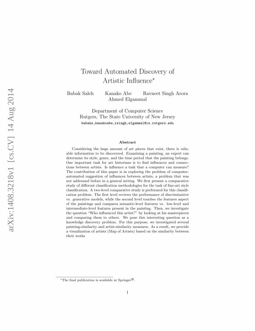
Toward Automated Discovery of

Artistic Influence∗

Babak Saleh Kanako Abe Ravneet Singh AroraAhmed Elgammal

Department of Computer ScienceRutgers, The State University of New Jerseybabaks,kanakoabe,rsingh,elgammal@cs.rutgers.edu

Abstract

Considering the huge amount of art pieces that exist, there is valu-able information to be discovered. Examining a painting, an expert candetermine its style, genre, and the time period that the painting belongs.One important task for art historians is to find influences and connec-tions between artists. Is influence a task that a computer can measure?The contribution of this paper is in exploring the problem of computer-automated suggestion of influences between artists, a problem that wasnot addressed before in a general setting. We first present a comparativestudy of different classification methodologies for the task of fine-art styleclassification. A two-level comparative study is performed for this classifi-cation problem. The first level reviews the performance of discriminativevs. generative models, while the second level touches the features aspectof the paintings and compares semantic-level features vs. low-level andintermediate-level features present in the painting. Then, we investigatethe question “Who influenced this artist?” by looking at his masterpiecesand comparing them to others. We pose this interesting question as aknowledge discovery problem. For this purpose, we investigated severalpainting-similarity and artist-similarity measures. As a result, we providea visualization of artists (Map of Artists) based on the similarity betweentheir works

∗The final publication is available at Springer R©.

1

arX

iv:1

408.

3218

v1 [

cs.C

V]

14

Aug

201

4

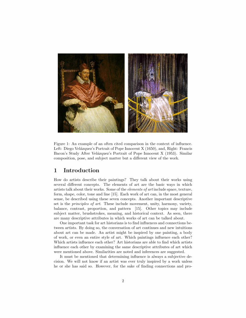
Figure 1: An example of an often cited comparison in the context of influence.Left: Diego Velazquez’s Portrait of Pope Innocent X (1650), and, Right: FrancisBacon’s Study After Velazquez’s Portrait of Pope Innocent X (1953). Similarcomposition, pose, and subject matter but a different view of the work.

1 Introduction

How do artists describe their paintings? They talk about their works usingseveral different concepts. The elements of art are the basic ways in whichartists talk about their works. Some of the elements of art include space, texture,form, shape, color, tone and line [15]. Each work of art can, in the most generalsense, be described using these seven concepts. Another important descriptiveset is the principles of art. These include movement, unity, harmony, variety,balance, contrast, proportion, and pattern [15]. Other topics may includesubject matter, brushstrokes, meaning, and historical context. As seen, thereare many descriptive attributes in which works of art can be talked about.

One important task for art historians is to find influences and connections be-tween artists. By doing so, the conversation of art continues and new intuitionsabout art can be made. An artist might be inspired by one painting, a bodyof work, or even an entire style of art. Which paintings influence each other?Which artists influence each other? Art historians are able to find which artistsinfluence each other by examining the same descriptive attributes of art whichwere mentioned above. Similarities are noted and inferences are suggested.

It must be mentioned that determining influence is always a subjective de-cision. We will not know if an artist was ever truly inspired by a work unlesshe or she has said so. However, for the sake of finding connections and pro-

2

gressing through movements of art, a general consensus is agreed upon if theargument is convincing enough. For example, Figure 1 illustrates a commonlycited comparison for studying influence, in the work of Francis Bacon’s StudyAfter Velazquez’s Portrait of Pope Innocent X (1953), where similarity is clearin composition, pose, and subject matter.

Is influence a task that a computer can measure? In the last decade therehave been impressive advances in developing computer vision algorithms fordifferent object recognition-related problems including: instance recognition,categorization, scene recognition, pose estimation, etc. When we look into animage we not only recognize object categories, and scene category, we can alsoinfer various aesthetic, cultural and historical aspects. For example, when welook at a fine-art paining, an expert, or even an average person can infer in-formation about the style of that paining (e.g. Baroque vs. Impressionism),the genre of the painting (e.g. a portrait or a landscape), or even can guessthe artist who painted it. People can look at two painting and find similaritiesbetween them in different aspects (composition, color, texture, subject matter,etc.) This is an impressive ability of human perception for learning and judg-ing complex aesthetic-related visual concepts, which for long have been thoughtnot to be a logical process. In contrast, we tackle this problem using a compu-tational methodology approach, to show that machines can in fact learn suchaesthetic concepts.

Although there has been some research on automated classification of paint-ings e.g. [2, 6, 7, 23, 17], however, there is almost no research done on computer-based measuring and determining of influence between artists. Measuring in-fluence is a very difficult task because of the broad criteria for what influencebetween artists can mean. As mentioned earlier, there are many different ways inwhich paintings can be described. Some of these descriptions can be translatedto a computer. For example, Li et al [23] proposed automated way for analyzingbrushstrokes to distinguish between Van Gogh and his contemporaries. For thepurpose of this paper, we do not focus on a specific element of art or princi-ple of art but instead we focus on finding and suggesting new comparisons byexperimenting with different similarity measures and features.

What is the benefit of the study of automated methods of analyzing paintingsimilarity and artistic influences? By including a computer quantified judgementabout which artists and paintings may have similarities, it not only finds newknowledge about which paintings are connected using a mathematical criteria,but also keeps the conversation going for artists. It challenges people to considerpossible connections in the timeline of art history that may have never beenseen before. We are not asserting truths but instead suggesting a possible pathtowards a difficult task of measuring influence.

Besides the scientific merit of the problem, there are various application-oriented motivations. With the increasing volumes of digitized art databases onthe internet comes the daunting task of organization and retrieval of paintings.There are millions of paintings present on the internet. To manage properlythe databases of these paintings, it becomes very essential to classify paintingsinto different categories and sub-categories. This classification structure can be

3

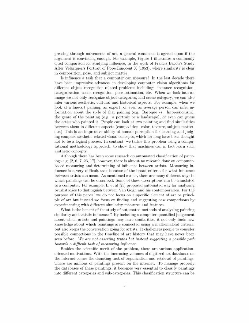
Figure 2: Frederic Bazille’s Studio 9 Rue de la Condamine (left) and NormanRockwell’s Shuffleton’s Barber Shop (right). The composition of both paintingsis divided in a similar way. Yellow circles indicate similar objects, red linesindicate composition, and the blue square represents similar structural element.The objects seen – a fire stove, three men clustered, chairs, and window are seenin both paintings along with a similar position in the paintings. After browsingthrough many publications and websites, we conclude that this comparison hasnot been made by an art historian before.

utilized as an index and thus can improve the speed of retrieval process. Also itwill be of great significance if we can infer new information about an unknownpainting using already existing databases of paintings, and as a broader viewcan infer high-level information like influences between painters.

Although the meaning of a painting is unique to each artist and is completelysubjective, it can somewhat be measured by the symbols and objects in thepainting. Symbols are visual words that often express something about themeaning of a work as well. For example, the works of Renaissance artists such asGiovanni Bellini and Jan Van-Eyck use religious symbols such as a cross, wings,and animals to tell stories in the Bible. This shows the need for an object-basedrepresentation of images. We should be able to describe the painting from a listof many different object classes. By having an object-based representation, theimage is described in a high-level semantic as opposed to low-level features suchas color and texture, which facilitates suggesting influences based on subjectmatter. Paintings do not necessarily have to look alike, but if they do, orhave reoccurring objects (high-level semantics), then they might be consideredsimilar. If influence is found by looking at similar characteristics of paintings,the importance of finding a good similarity measure becomes prominent. Timeis also an essential factor in determining influence. An artist cannot influenceanother artist in the past. Therefore the linearity of paintings cuts down thepossibilities of influence.

The contribution of this paper is in exploring the problem of computer-

4

automated suggestion of influences between artists, a problem that was notaddressed before in a general setting. From a machine-learning point of view,we approach the problem as an unsupervised knowledge discovery problem.Our methodology is based on three components: 1) studying different repre-sentations of painting to determine which is more useful for the task of influ-ence detection; 2) measuring similarity between paintings; 3) studying differentmeasures of similarity between artists. We collected a comprehensive paintingdataset for conducting our study. The data set contains 1710 high-resolutionimages of paintings by 66 artist spanning the time period of 1412-1996 andcontaining 13 painting styles. We also collect a ground-truth data set for thetask of artistic influences, which mainly contains positive influences claimed byart historian. This ground-truth is only used for the overall evaluation of ourdiscovered/suggested influences, and is not used in the learning or knowledge-discovery.

We hypothesis that a high-level semantic representation of painting wouldbe more useful for the task of influence detection. However, evaluating sucha hypothesis requires comparing the performance of different features and rep-resentation in detecting influences against a ground-truth of artistic influences,containing both positive and negative example. However, because of the limitedsize of the available ground-truth data, and the lack of negative examples in it,it is not useful for comparing different features and representations. Instead weresort to a highly correlated task, which is classifying painting style. The hy-pothesis is that features and representations that are good for style classification(which is a supervised learning problem), would also be good for determininginfluences (which is an unsupervised problem). Therefore, we performed a com-prehensive comparative study of different features and classification models forthe task of classifying painting style among seven different styles. This study isdescribed in details in Sec 4. The conclusion of this study confirms our hypoth-esis that high-level semantic features would be more useful for the task of styleclassification, and hence useful for determining influences.

Using the right features to represent the painting paves the way to judge sim-ilarity between paintings in a quantifiable way. Figure 2 illustrates an exampleof similar paintings detected by our automated methodology; Frederic Bazille’sStudio 9 Rue de la Condamine (1870) and Norman Rockwell’s Shuffleton’s Bar-ber Shop (1950). After browsing through many publications and websites, weconcluded, to the best of our knowledge, that this comparison has not beenmade by an art historian before. The painting might not look similar at thefirst glance, however, a closer look reveals striking similarity in composition andsubject matter, that is detected by our automated methodology (see caption fordetails). Other example similarity can be seen in Figures 7 & 8.

Measuring similarity between painting is fundamental to discover influences,however, it is not clear how painting similarity might be used to suggest influ-ences between artist. The paintings of a given artist can span extended periodof time and can be influenced by several other contemporary and prior artists.Therefore, we investigated several artist distance measures to judge similarity intheir work and suggest influences. As a result of this distance measures, we can

5

achieve visualizations of how artists are similar to each other, which we denoteby a map of artists.

The paper is structured as follows: Section 2 provides a literature survey onthe topic of computer-based methods for analyzing painting. Section 3 describesthe data set used in our study. Section 4 describes our comparative study for thetask of painting style classification, including the methodologies, features andthe results. Section 5 describes our methodology for judging artistic influence.Section 6 represents qualitative and quantitative evaluation of our automatedinfluence study.

2 Related Works

There is little work done in the area of automated fine-art classification. Mostof the work done in the problem of paintings classification utilizes low-levelfeatures such as color, shades, texture and edges. Lombardi [24] presented acomprehensive study of the performance of such features for paintings classi-fication. In that paper the style of the painting was identified as a result ofrecognizing the painter. Sablatnig et al. [28] used brushstroke patterns to definestructural signature to identify the artist style. Khan et al. [13] used a Bag ofWords (BoW) approach with low-level features of color and shades to identifythe painter among eight different artists. In [29] and [20] similar experimentswith low-level features were conducted. Unlike most of the previous works thatfocused on inferring the artist from the painting, our goal is to directly recognizethe style of the painting, and discover artist similarity and influences, which aremore challenging tasks.

Carneiro et al. [8] recently published the dataset “PRINTART” on paint-ings along with primarily experiments on image retrieval and painting styleclassification. They provided three levels of annotation for the “PRINTART”dataset: Global, Local and Pose annotation. However this dataset contains onlymonochromatic artistic images. We present a new dataset which has chromaticimages and its size is about double the “PRINTART” dataset covering a morediverse set of styles and topics. Carneiro et al. [8] showed that the low-leveltexture and color features exploited for photographic image analysis are not aseffective because of inconsistent color and texture patterns describing the visualclasses (e.g. humans) in artistic images.

Carneiro et al. [8] define artistic image understanding as a process that re-ceives an artistic image and outputs a set of global, local and pose annotations.The global annotations consist of a set of artistic keywords describing the con-tents of the image. Local annotations comprise a set of bounding boxes thatlocalize certain visual classes, and pose annotations consisting of a set of bodyparts that indicate the pose of humans and animals in the image. Anotherprocess involved in the artistic image understanding is the retrieval of imagesgiven a query containing an artistic keyword. In. [8] an improved inverted labelpropagation method was proposed that produced the best results, both in theautomatic (global, local and pose) annotation and retrieval problems.

6

Carneiro et. al. [7] targeted the problem of annotating an unseen image witha set of global labels, learned on top of annotated paintings. Furthermore, fora given set of visual classes, they are able to retrieve the painting which showsthe same characteristics. They have proposed a graph-based learning algorithmbased on the assumption that visually similar paintings share same annotation.They formulated the global annotation problem with a combinatorial harmonicapproach, which computes the probability that a random walk starting at thetest image first reaches each of the database samples. However all the samplesare from fifteen to seventeen century and focused on religious themes.

Graham et. al. [17] posed the question of finding the way we perceive two art-work as similar to each other. Toward this goal, they acquired strong supervisionof human experts to label similar paintings. They apply multidimensional scal-ing methods to paired similar paintings from either Landscape or portrait/stilllife and showed that similarity between paintings can be interpreted as basicimage statistics. In the experiments they show that for landscape paintings,basic grey image statistics is the most important factor for two artwork to besimilar. For the case of still life/portrait most important elements of similarityare semantic variables, for example representation of people.

Unlike the case of ordinary images, where color and texture are proper low-level features to be used for a diverse set of tasks (e.g. classification), thesemight not describe paintings well. Color and texture features are highly proneto variations during digitization of paintings. In the case of color, it also lacksfidelity due to aging. The effect of digitization on the computational analysis ofpaintings is investigated in great depth by Polatkan et. al [18].

The aforementioned reasons make the brushstrokes more meaningful featuresfor describing paintings. Li et al. [23] used fully automatic extracted brush-strokes to describe digitized paintings. Their novel feature extraction methodis developed by the integration of edge detection and clustering-based segmen-tation. Using these features they found that regularly shaped brushstrokes aretightly arranged, creating a repetitive and patterned impression that can repre-sent Van Gogh style and help to distinguish his work from his contemporaries.They have conducted a set of analysis based on 45 digitized oil paintings ofVan Gogh from museum’s collections. Due to small number of samples, and toavoid overfitting, they state this problem as a hypothesis testing rather thanclassification. They hypothesize which factors are eminent in Van Gogh stylecomparing to his contemporaries and tested them by statistical approaches ontop of brushstroke features.

Cabral et al [6] approached the problem of ordering paintings and estimatingtheir time period. They formulated this problem as embedding paintings into aone dimensional manifold and tried two different methods: on one hand, theyapplied unsupervised embedding using Laplacian Eignemaps [3]. To do so theyonly need visual features and defined a convex optimization to map paintingsto a manifold. This approach is very fast and do not need human expertise,but its accuracy is low. On the other hand, since some partial ordering onpaintings is available by experts, they use these information as a constraint andused Maximum Variance Unfolding [36] to find a proper space, capturing more

7

accurate ordering of paintings.

3 Dataset

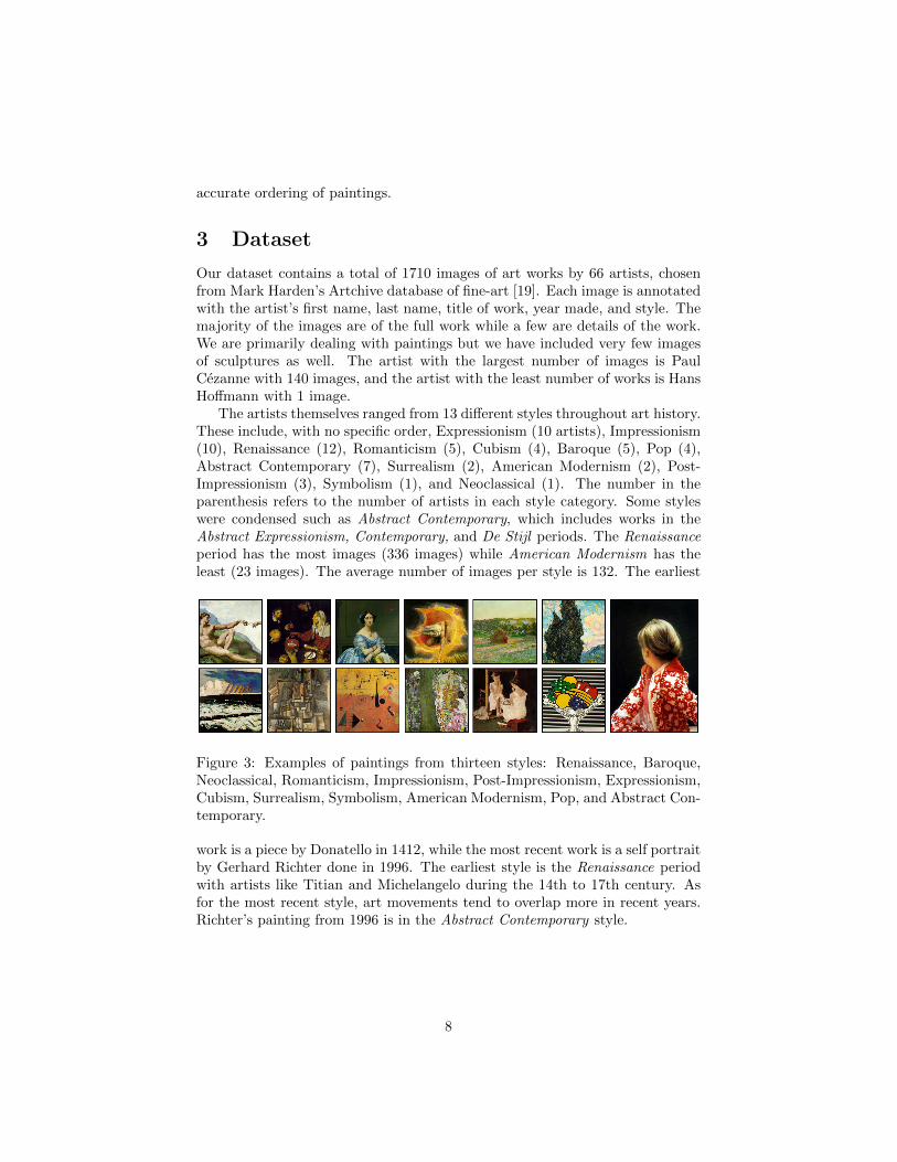
Our dataset contains a total of 1710 images of art works by 66 artists, chosenfrom Mark Harden’s Artchive database of fine-art [19]. Each image is annotatedwith the artist’s first name, last name, title of work, year made, and style. Themajority of the images are of the full work while a few are details of the work.We are primarily dealing with paintings but we have included very few imagesof sculptures as well. The artist with the largest number of images is PaulCezanne with 140 images, and the artist with the least number of works is HansHoffmann with 1 image.

The artists themselves ranged from 13 different styles throughout art history.These include, with no specific order, Expressionism (10 artists), Impressionism(10), Renaissance (12), Romanticism (5), Cubism (4), Baroque (5), Pop (4),Abstract Contemporary (7), Surrealism (2), American Modernism (2), Post-Impressionism (3), Symbolism (1), and Neoclassical (1). The number in theparenthesis refers to the number of artists in each style category. Some styleswere condensed such as Abstract Contemporary, which includes works in theAbstract Expressionism, Contemporary, and De Stijl periods. The Renaissanceperiod has the most images (336 images) while American Modernism has theleast (23 images). The average number of images per style is 132. The earliest

Figure 3: Examples of paintings from thirteen styles: Renaissance, Baroque,Neoclassical, Romanticism, Impressionism, Post-Impressionism, Expressionism,Cubism, Surrealism, Symbolism, American Modernism, Pop, and Abstract Con-temporary.

work is a piece by Donatello in 1412, while the most recent work is a self portraitby Gerhard Richter done in 1996. The earliest style is the Renaissance periodwith artists like Titian and Michelangelo during the 14th to 17th century. Asfor the most recent style, art movements tend to overlap more in recent years.Richter’s painting from 1996 is in the Abstract Contemporary style.

8

4 Painting-Style Classification: A ComparativeStudy

In this section we present the details of our study on painting style classification.The problem of painting style classification can be stated as: Given a set ofpaintings for each painting style, predict the style of an unknown painting. Alot of work has been done so far on the problem of image category recognition,however the problem of painting classification proves quite different than that ofimage category classification. Paintings are differentiated, not only by contents,but also by style applied by a particular painter or school of painting or by theage when they were painted. This makes painting classification problem muchmore challenging than the ordinary image category recognition problem.

In this study we will approach the problem of painting style classificationfrom a supervised learning perspective. A two-level comparative study is con-ducted for this classification problem. The first level reviews the performance ofdiscriminative vs. generative models, while the second level touches the featureaspects of the paintings and compares semantic-level features vs. low-level andintermediate-level features present in the painting.

For experimental purposes seven fine-art styles are used, namely Renais-sance, Baroque, Impressionism, Cubism, Abstract, Expressionism, and Popart.Various different sets of comparative experiments were performed focused onevaluation of classification accuracy for each methodology. We evaluated threedifferent methodologies, namely:

1. Discriminative model using a Bag-of-Words (BoW) approach

2. Generative model using BoW

3. Discriminative model using Semantic-level features

As shown in Figure 4, these three models differ in terms of the classificationmethodology, as well as the type of features used to represent the painting. TheDiscriminative Semantic-Level model applies a discriminative machine learningmodel upon features capturing semantic information present in a painting, whileDiscriminative and Generative BoW models employs discriminative and gener-ative machine learning models, respectively, on the Intermediate level featuresrepresented using a BoW model.

A generative model has the property that it specifies a joint probability dis-tribution over observed samples and their labels. In other words, a generativeclassifier learns a model of joint probability distribution p(x, y), where x de-notes the observed samples and y are the labels. Bayes rule can be appliedto predict the label y for a given new sample x, which is determined by theprobability distribution p(y|x). Since a generative model calculates the distri-bution p(x|y) as an intermediate step, these can be used to generate randominstances x conditioned on target labels y. A discriminative model, in contrast,tries to estimate the distribution p(y|x) directly from the training data. Thus,

9

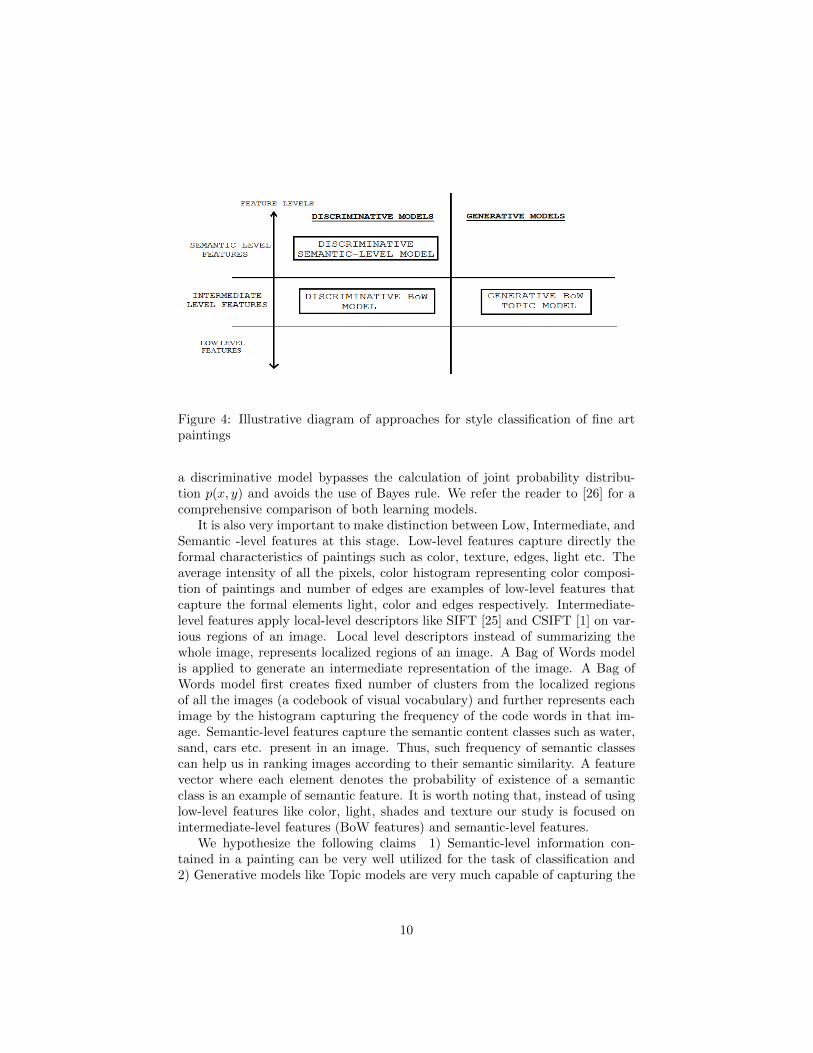
Figure 4: Illustrative diagram of approaches for style classification of fine artpaintings

a discriminative model bypasses the calculation of joint probability distribu-tion p(x, y) and avoids the use of Bayes rule. We refer the reader to [26] for acomprehensive comparison of both learning models.

It is also very important to make distinction between Low, Intermediate, andSemantic -level features at this stage. Low-level features capture directly theformal characteristics of paintings such as color, texture, edges, light etc. Theaverage intensity of all the pixels, color histogram representing color composi-tion of paintings and number of edges are examples of low-level features thatcapture the formal elements light, color and edges respectively. Intermediate-level features apply local-level descriptors like SIFT [25] and CSIFT [1] on var-ious regions of an image. Local level descriptors instead of summarizing thewhole image, represents localized regions of an image. A Bag of Words modelis applied to generate an intermediate representation of the image. A Bag ofWords model first creates fixed number of clusters from the localized regionsof all the images (a codebook of visual vocabulary) and further represents eachimage by the histogram capturing the frequency of the code words in that im-age. Semantic-level features capture the semantic content classes such as water,sand, cars etc. present in an image. Thus, such frequency of semantic classescan help us in ranking images according to their semantic similarity. A featurevector where each element denotes the probability of existence of a semanticclass is an example of semantic feature. It is worth noting that, instead of usinglow-level features like color, light, shades and texture our study is focused onintermediate-level features (BoW features) and semantic-level features.

We hypothesize the following claims 1) Semantic-level information con-tained in a painting can be very well utilized for the task of classification and2) Generative models like Topic models are very much capable of capturing the

10

thematic structure of a painting. It is easy to visualize a topic or theme in thecase of documents. For documents, a topic can be a collection of particularset of words. For example, a science topic is characterized by the collectionof words like atom, electrons, protons etc. For images represented by a Bagof Word model, each word is represented by the local level descriptor used todescribe the image. Thus a collection of particular set of such similar regionscan constitute a topic. For example, collection of regions representing mainlystraight edges can constitute the topic trees. Similarly, set of regions havinghigh concentration of blue color can form up a theme related to sky or water.

The following subsections describe the details of the compared methodolo-gies.

4.1 Discriminative Bag-of-Words model

Bag of Words(BoW) [31] is a very popular model in text categorization torepresent documents, where the order of the words does not matter. BoWwas successfully adapted for object categorization, e.g. in [16, 33, 37]. Typicalapplication of BoW on an image involves several steps, which includes:

1) Locating interest points in an image

2) Representation of such points/regions using feature descriptors

3) Codebook formation using K-Means clustering, to obtain a “dictionary” ora codebook of visual words.

4) Vector quantization of the feature descriptor; each descriptor is encoded byits nearest visual word from the codebook.

5) Generate an intermediate-level representations for each image using thecodebook, in the form of a histogram of the visual words present in eachimage.

6) Train a discriminative classifier on the intermediate training feature vectorsfor each class.

7) For classification, the trained classifier is applied on the BoW feature vectorof a test image.

Thus, the end result of a Bag of Words model is a histogram of words, whichis used as an intermediate-level feature to represent a painting. In our study, weapplied a Support Vector Machine (SVM) classifier [5] on a code-book trainedon images from our dataset. We used two variant of the widely used ScaleInvariant Feature Transform “SIFT” features [25] called Color SIFT (CSIFT) [1]and opponent SIFT (OSIFT) [22] as local features. The SIFT [25] is invariant toimage scale, rotation, affine distortion and illumination. It uses edge orientationsto define a local region and also utilizes the gradient of an image. Also, theSIFT descriptor is normalized and hence is also immune to gradient magnitudechanges. CSIFT [1] and opponent SIFT (OSIFT) [22] extends SIFT features

11

for color images, which is essential for the task of painting-style classification.In an earlier study by Van De Sande et al [35] opponent SIFT was shown tooutperform other color SIFT variants in image categorization tasks.

4.2 Discriminative Semantic-level model

In this approach a discriminative model is employed on top of semantic-levelfeatures. Seeking semantic-level features, we extracted the Classeme featurevector [34] as the visual feature for each painting. Classeme features are outputof a set of classifiers corresponding to a set of C category labels, which are drawnfrom an appropriate term list, defined in [34], and not related to our fine-artcontext. For each category c ∈ {1 · · ·C}, a set of training images was gatheredby issuing a query on the category label to an image search engine. After aset of coarse feature descriptors (Pyramid HOG, GIST) is extracted, a subsetof feature dimensions was selected [34]. Using this reduced dimension features,a one-versus-all classifier φc is trained for each category. The classifier outputis real-valued, and is such that φc(x) > φc(y) implies that x is more similarto class c than y is. Given an image x, the feature vector (descriptor) used torepresent it is the Classeme vector [φ1(x), · · · , φC(x)]. The Classeme feature isof dimensionality N = 2569.

We used such feature vectors to train a Support Vector Machine (SVM) [5]classifier for each painting genre. We hypothesize that Classeme features aresuitable for representing and summarizing the overall contents of a paintingsince it captures semantic-level information about object presence in a paintingencoded implicitly in the output of the pre-trained classifiers.

4.3 Generative Bag-of-Words Topic model

Generative topic model uses Latent Dirichlet Allocation (LDA) [10]. In stud-ies [14] and [21], LDA and Probabilistic Latent Semantic Analysis (pLSA) topicmodels have been applied for object categorization, localization and scene cat-egorization. This paper is the first evaluation of such models in the domain offine-art categorization.

For the purpose of our study, we used Latent Dirichlet Allocation (LDA [10])topic model and applied it on BoW representation of paintings using bothCSIFT and OSIFT features. In LDA, each item is represented by a finite mix-ture over a set of topics and each topic is characterized by a distribution overwords. Figure 4.3 shows a graphical model for the image generation process. Asshown in the model, parameter Θ defines the topic distribution for each image(total number of images is D.) Θ is determined by Dirichlet parameter α, β andrepresents the word distribution for each topic. The total number of words isN. To use LDA for the classification task, we build model for each of the stylesin our framework. First step is to represent each training image by a quan-tized vector using Bag-of-Words model described earlier. This vector quantizedrepresentation of each image is used for parameter estimation using VariationalInference. Thus, we will get LDA parameters Θc and βc for each category c.

12

W Z θ α

N D

β

Figure 5: Graphical model representing Latent Dirichlet Allocation

Confusion(%) Baroque Abstract Renaissance Pop-Art Expressionism Impressionism CubismBaroque 87.5 0 14.3 0 5.3 17.8 1.78Abstract 0 64 0 7.1 7.1 1.8 1.9Renaissance 5.4 0 64.3 5.35 14.3 3.5 1.8Pop-Art 0 1.78 1.8 73.1 0 3.5 1.8Expressionism 1.8 20.2 7.1 3.6 48.2 17.8 12.9Impressionism 5.36 8 9 5.3 17.8 48.2 9.2Cubism 0 6 3.5 5.3 7.1 7.1 72.4

Table 1: Confusion matrix for Discriminative Semantic Model

Once we have a new test image, d, we can infer the parameter Θcd for eachcategory and p(d|Θcd, βc) is used as the likelihood of the image belonging to aparticular class c.

4.4 Style Classification Results

For the task of Style classification of paintings, we focus on a subset of ourdataset that contains seven categories of paintings namely Abstract, Baroque,Renaissance, Pop-art, Expressionism, Impressionism and Cubism. Each cate-gory consists of 70 paintings. For each of the following experiments five-foldcross-validation was performed, with 20% of the images chosen for testing pur-pose in each fold.

For codebook formation, Harris-Laplace detector [30] is used to find theinterest points. For efficient computation the number of interest points foreach painting is restricted to 3000. Standard K-means Clustering algorithm isused to build a Codebook of size 600 words. SVM classifier is trained on bothintermediate-level and semantic-level descriptors. For SVM, we use Radial Ba-sis function (RBF) kernels. To determine parameters for the SVM, the gridsearch algorithm implemented by [9] is employed. Grid search algorithm usescross-validation to pick up the optimum parameter values. Also this process ispreceded by scaling of dataset descriptors. For experiments with LDA, DavidBeli’s C-code [10] is used for the task of parameter estimation and inference.

13

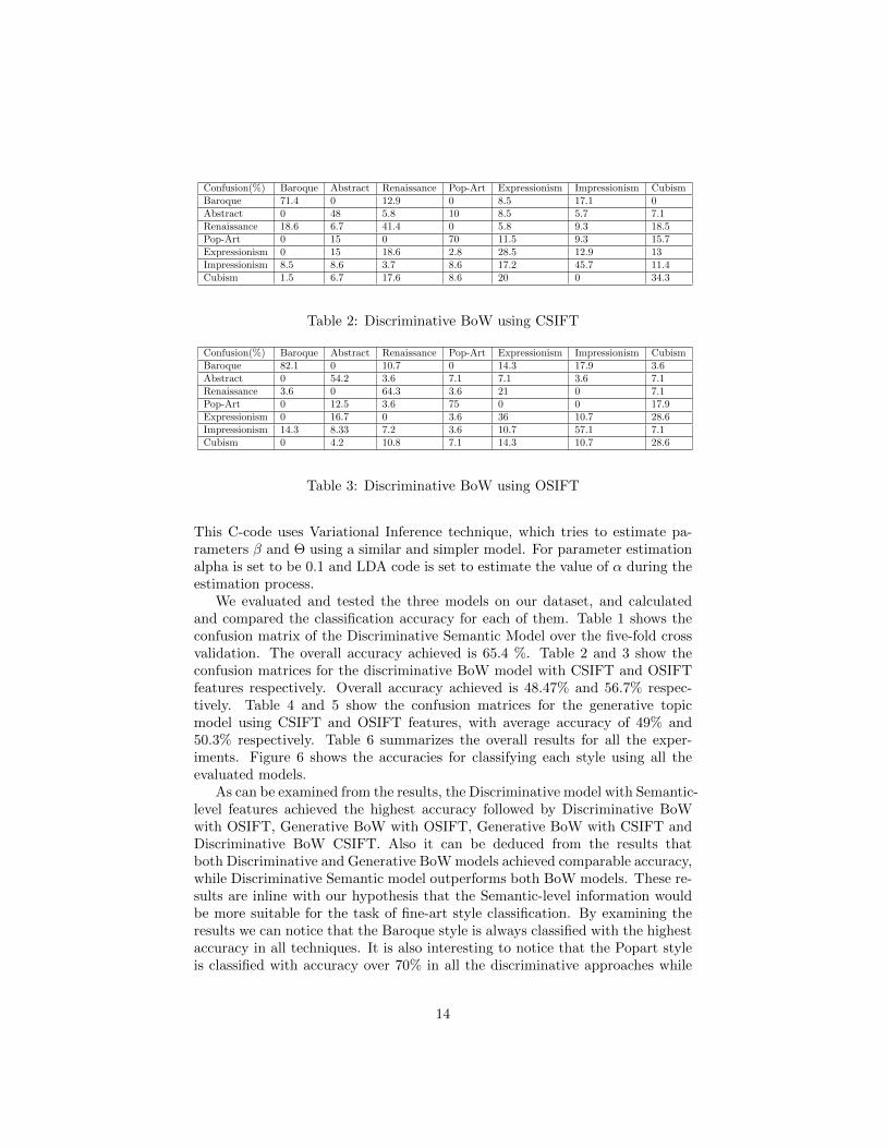
Confusion(%) Baroque Abstract Renaissance Pop-Art Expressionism Impressionism CubismBaroque 71.4 0 12.9 0 8.5 17.1 0Abstract 0 48 5.8 10 8.5 5.7 7.1Renaissance 18.6 6.7 41.4 0 5.8 9.3 18.5Pop-Art 0 15 0 70 11.5 9.3 15.7Expressionism 0 15 18.6 2.8 28.5 12.9 13Impressionism 8.5 8.6 3.7 8.6 17.2 45.7 11.4Cubism 1.5 6.7 17.6 8.6 20 0 34.3

Table 2: Discriminative BoW using CSIFT

Confusion(%) Baroque Abstract Renaissance Pop-Art Expressionism Impressionism CubismBaroque 82.1 0 10.7 0 14.3 17.9 3.6Abstract 0 54.2 3.6 7.1 7.1 3.6 7.1Renaissance 3.6 0 64.3 3.6 21 0 7.1Pop-Art 0 12.5 3.6 75 0 0 17.9Expressionism 0 16.7 0 3.6 36 10.7 28.6Impressionism 14.3 8.33 7.2 3.6 10.7 57.1 7.1Cubism 0 4.2 10.8 7.1 14.3 10.7 28.6

Table 3: Discriminative BoW using OSIFT

This C-code uses Variational Inference technique, which tries to estimate pa-rameters β and Θ using a similar and simpler model. For parameter estimationalpha is set to be 0.1 and LDA code is set to estimate the value of α during theestimation process.

We evaluated and tested the three models on our dataset, and calculatedand compared the classification accuracy for each of them. Table 1 shows theconfusion matrix of the Discriminative Semantic Model over the five-fold crossvalidation. The overall accuracy achieved is 65.4 %. Table 2 and 3 show theconfusion matrices for the discriminative BoW model with CSIFT and OSIFTfeatures respectively. Overall accuracy achieved is 48.47% and 56.7% respec-tively. Table 4 and 5 show the confusion matrices for the generative topicmodel using CSIFT and OSIFT features, with average accuracy of 49% and50.3% respectively. Table 6 summarizes the overall results for all the exper-iments. Figure 6 shows the accuracies for classifying each style using all theevaluated models.

As can be examined from the results, the Discriminative model with Semantic-level features achieved the highest accuracy followed by Discriminative BoWwith OSIFT, Generative BoW with OSIFT, Generative BoW with CSIFT andDiscriminative BoW CSIFT. Also it can be deduced from the results thatboth Discriminative and Generative BoW models achieved comparable accuracy,while Discriminative Semantic model outperforms both BoW models. These re-sults are inline with our hypothesis that the Semantic-level information wouldbe more suitable for the task of fine-art style classification. By examining theresults we can notice that the Baroque style is always classified with the highestaccuracy in all techniques. It is also interesting to notice that the Popart styleis classified with accuracy over 70% in all the discriminative approaches while

14

Confusion(%) Baroque Abstract Renaissance Pop-Art Expressionism Impressionism CubismBaroque 86.6 0 14.3 0 14.3 7.1 7.1Abstract 0 58.3 7.1 26.6 0 7.1 14.3Renaissance 6.6 8.3 42.8 20 14.3 0 7.1Pop-Art 0 0 7.1 13.3 0 0 14.3Expressionism 0 8.3 7.1 6.6 36 14.3 7.1Impressionism 6.6 25 14.3 13.3 21.4 71.4 14.3Cubism 0 0 7.1 20 14.3 0 35.7

Table 4: Generative BoW topic model using CSIFT

Confusion(%) Baroque Abstract Renaissance Pop-Art Expressionism Impressionism CubismBaroque 75.5 0 14.3 0 3.6 10.7 7.1Abstract 0 62.5 3.5 27.3 3.6 3.6 0Renaissance 7.1 4.2 39.2 3.3 7.1 3.6 10.7Pop-Art 0 8.3 0 28 3.6 0 7.1Expressionism 7.1 0 17.8 14 36 3.6 10.7Impressionism 10.2 25 10.7 10.2 32 68 21.4Cubism 0 0 14.3 16.9 14.3 10.7 42.9

Table 5: Generative BoW topic model using OSIFT

the generative approach performed poorly in that style. Also it is worth notingthat the OSIFT features outperformed the CSIFT features in the discriminativecase; however the difference is not significant in the generative case.

5 Influence Discovery Framework

Consider a set of artists, denoted by A = {al, l = 1 · · ·Na}, where Na is thenumber of artists. For each artist, al, we have a set of images of paintings,denoted by P l = {pli, i = 1, · · · , N l}, where N l is the number of paintingsfor the l-th artist. For clarity of the presentation, we reserve the superscriptfor the artist index and the subscript for the painting index. We denote byN =

∑lNl the total number of paintings. Following the conclusion of the style

classification comparative study, we represent each painting by its Classemefeatures [34]. Therefore, each image pli ∈ RD is a D dimensional feature vectorthat is the outcome of the Classeme classifiers, which defines the feature space.

To represent the temporal information, for each artist we have a ground truthtime period where he/she performed their work, denoted by tl = [tlstart, t

lend]

for the l-th artist, where tlstart and tlend are the start and end year of that timeperiod respectively. We do not consider the date of a given painting since for

Model Dis Semantic Dis BoW CSIFT Dis BoW OSIFT Gen BoW CSIFT Gen BoW OSIFTMean Accuracy(%) 65.4 48.47 56.7 49 50.3Std 4.8 2.45 3.26 2.43 2.46

Table 6: Generative BoW topic model using OSIFT

15

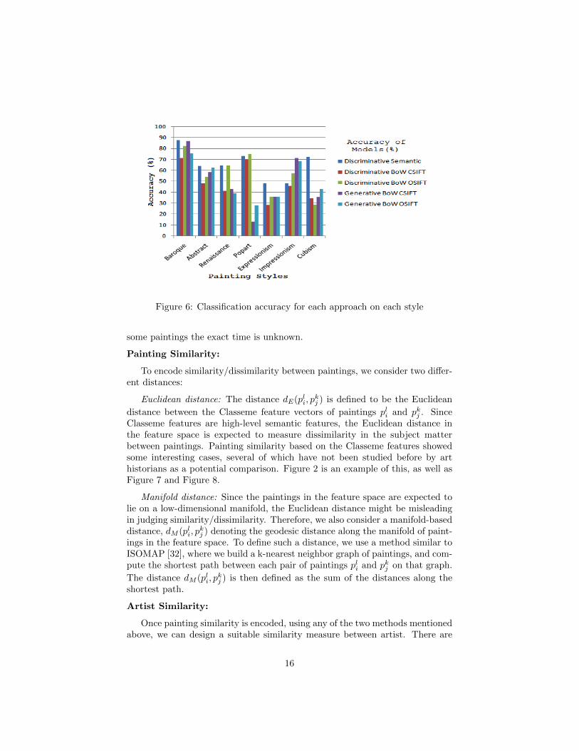
!Figure 6: Classification accuracy for each approach on each style

some paintings the exact time is unknown.

Painting Similarity:

To encode similarity/dissimilarity between paintings, we consider two differ-ent distances:

Euclidean distance: The distance dE(pli, pkj ) is defined to be the Euclidean

distance between the Classeme feature vectors of paintings pli and pkj . SinceClasseme features are high-level semantic features, the Euclidean distance inthe feature space is expected to measure dissimilarity in the subject matterbetween paintings. Painting similarity based on the Classeme features showedsome interesting cases, several of which have not been studied before by arthistorians as a potential comparison. Figure 2 is an example of this, as well asFigure 7 and Figure 8.

Manifold distance: Since the paintings in the feature space are expected tolie on a low-dimensional manifold, the Euclidean distance might be misleadingin judging similarity/dissimilarity. Therefore, we also consider a manifold-baseddistance, dM (pli, p

kj ) denoting the geodesic distance along the manifold of paint-

ings in the feature space. To define such a distance, we use a method similar toISOMAP [32], where we build a k-nearest neighbor graph of paintings, and com-pute the shortest path between each pair of paintings pli and pkj on that graph.

The distance dM (pli, pkj ) is then defined as the sum of the distances along the

shortest path.

Artist Similarity:

Once painting similarity is encoded, using any of the two methods mentionedabove, we can design a suitable similarity measure between artist. There are

16

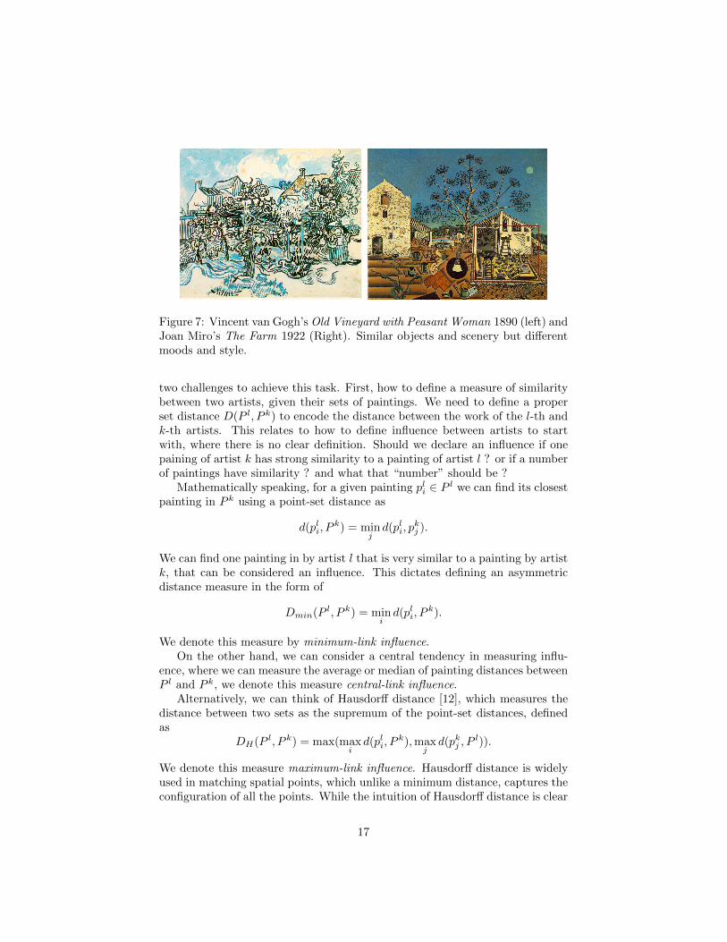
Figure 7: Vincent van Gogh’s Old Vineyard with Peasant Woman 1890 (left) andJoan Miro’s The Farm 1922 (Right). Similar objects and scenery but differentmoods and style.

two challenges to achieve this task. First, how to define a measure of similaritybetween two artists, given their sets of paintings. We need to define a properset distance D(P l, P k) to encode the distance between the work of the l-th andk-th artists. This relates to how to define influence between artists to startwith, where there is no clear definition. Should we declare an influence if onepaining of artist k has strong similarity to a painting of artist l ? or if a numberof paintings have similarity ? and what that “number” should be ?

Mathematically speaking, for a given painting pli ∈ P l we can find its closestpainting in P k using a point-set distance as

d(pli, Pk) = min

jd(pli, p

kj ).

We can find one painting in by artist l that is very similar to a painting by artistk, that can be considered an influence. This dictates defining an asymmetricdistance measure in the form of

Dmin(P l, P k) = minid(pli, P

k).

We denote this measure by minimum-link influence.On the other hand, we can consider a central tendency in measuring influ-

ence, where we can measure the average or median of painting distances betweenP l and P k, we denote this measure central-link influence.

Alternatively, we can think of Hausdorff distance [12], which measures thedistance between two sets as the supremum of the point-set distances, definedas

DH(P l, P k) = max(maxid(pli, P

k),maxjd(pkj , P

l)).

We denote this measure maximum-link influence. Hausdorff distance is widelyused in matching spatial points, which unlike a minimum distance, captures theconfiguration of all the points. While the intuition of Hausdorff distance is clear

17

Figure 8: Georges Braque’s Man with a Violin 1912 (Left) and Pablo Picasso’sSpanish Still Life: Sun and Shadow 1912 (Right).

from a geometrical point of view, it is not clear what it means in the context ofartist influence, where each point represent a painting. In this context, Hausdorffdistance measures the maximum distance between any painting and its closestpainting in the other set.

The discussion above highlights the challenge in defining the similarity be-tween artists, where each of the suggested distance is in fact meaningful, andcaptures some aspects of similarity, and hence influence. In this paper, we donot take a position in favor of any of these measures, instead we propose to usea measure that can vary through the whole spectrum of distances between twosets of paintings. We define asymmetric distance between artist l and artist kas the q-percentile Hausdorff distance, as

Dq%(P l, P k) =q%

maxid(pli, P

k). (1)

Varying the percentile q allows us to evaluate different settings ranging from aminimum distance, Dmin, to a central tendency, to a maximum distance as inHausdorff distance DH .

Artist Influence Graph:

The artist asymmetric distance is used, in conjunction with the ground-truth time period to construct an influenced-by graph. The influence graph is adirected graph where each artist is represented by a node. A weighted directededge between node i and node j indicates that artist i is potentially influenced

18

by artist j, which is only possible if artist i succeed or is contemporary to artistj. The weight corresponds to the artist distance, i.e., a smaller weight indicatesa higher potential influence. Therefore, the graph weights are defined as

wij =

{Dq%(P i, P j) if tiend ≥ t

jstart

∞ otherwise(2)

6 Influence Discovery Results

6.1 Evaluation Methodology:

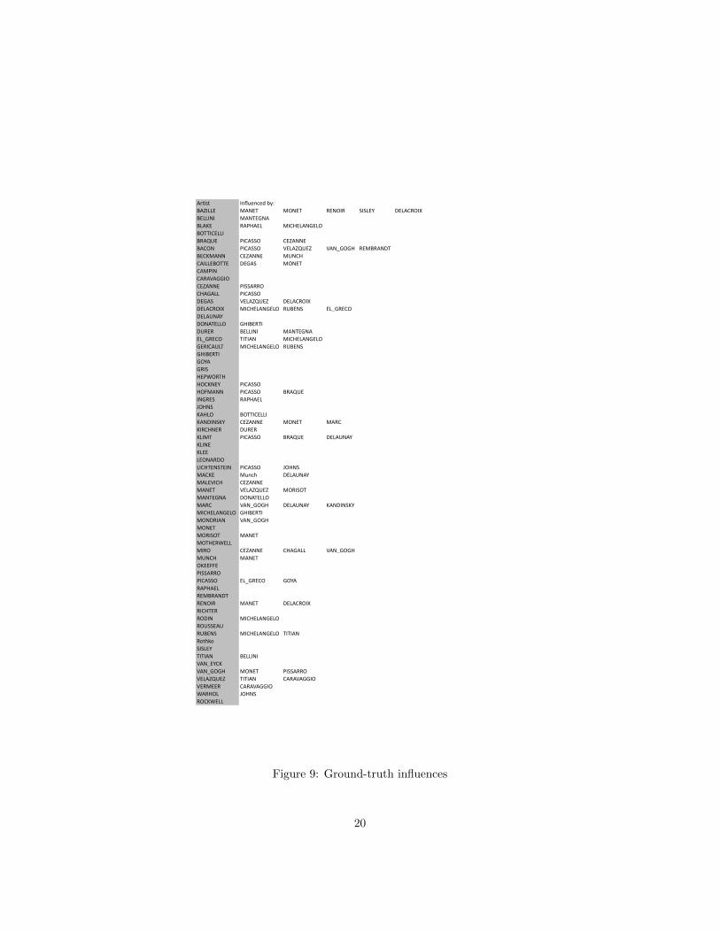
We researched known influences between artists within our dataset from multipleresources such as The Art Story Foundation and The Metropolitan Museum ofArt. For example, there is a general consensus among art historians that PaulCezanne’s use of fragmented spaces had a large impact on Pablo Picasso’s work.In total, we collected 76 pairs of one-directional artist influences, where a pair(ai, aj) indicates that artist i is influenced by artist j. Figure 9 shows thecomplete list of influenced-by list. Generally, it is a sparse list that containsonly the influences which are consensual among many. Some artists do not haveany influences in our collection while others may have up to five. We use thislist as ground-truth for measuring the accuracy in our experiments.

The constructed influenced-by graph is used to retrieve the top-k potentialinfluences for each artist. If a retrieved influence pair concur with an influenceground-truth pair, this is considered a hit. The hits are used to compute therecall, which is defined as the ratio between the correct influence detected andthe total known influences in the ground truth. The recall is used for the sakeof comparing the different settings relatively. Since detected influences can becorrect although not in our ground truth, so there is no meaning to computethe precision.

6.2 Influence Discovery Validation

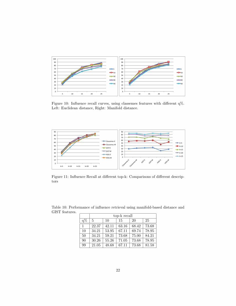
We experimented with the Classeme features, which showed the best results inthe style classification task. We also experimented with GIST descriptors [27]and HOG descriptors [11], since they are the main ingredients in the Classemesfeatures. In all cases, we computed the recall figures using the influence graphfor the top-k similar artist (k=5, 10, 15, 25) with different q-percentile for theartist distance measure in Eq 1 (q=1, 10, 50, 90, 99%). For all descriptors, wecomputed the influences using both the Euclidean distance and the Manifold-based distances. The results are shown in Tables 6.2- 6.2. The rows of thetables show different q-percentile. The columns show the recall percentage forthe top-k similar artists . From the difference results we can see that most ofthe time the 50%-set distance (central-link influence) gives better results. Wecan also notice that generally the manifold-based distance slightly out performsthe Euclidean distance for the same feature. Figure 10 shows the recall curvesusing the Classemes features with different q%. Figure 11 compares the recall

19

Ar#st Influenced  by:BAZILLE MANET MONET RENOIR SISLEY DELACROIXBELLINI MANTEGNABLAKE RAPHAEL MICHELANGELOBOTTICELLIBRAQUE PICASSO CEZANNEBACON PICASSO VELAZQUEZ VAN_GOGH REMBRANDTBECKMANN CEZANNE MUNCHCAILLEBOTTE DEGAS MONETCAMPINCARAVAGGIOCEZANNE PISSARROCHAGALL PICASSODEGAS VELAZQUEZ DELACROIXDELACROIX MICHELANGELO RUBENS EL_GRECODELAUNAYDONATELLO GHIBERTIDURER BELLINI MANTEGNAEL_GRECO TITIAN MICHELANGELOGERICAULT MICHELANGELO RUBENSGHIBERTIGOYAGRISHEPWORTHHOCKNEY PICASSOHOFMANN PICASSO BRAQUEINGRES RAPHAELJOHNSKAHLO BOTTICELLIKANDINSKY CEZANNE MONET MARCKIRCHNER DURERKLIMT PICASSO BRAQUE DELAUNAYKLINEKLEELEONARDOLICHTENSTEIN PICASSO JOHNSMACKE Munch DELAUNAYMALEVICH CEZANNEMANET VELAZQUEZ MORISOTMANTEGNA DONATELLOMARC VAN_GOGH DELAUNAY KANDINSKYMICHELANGELO GHIBERTIMONDRIAN VAN_GOGHMONETMORISOT MANETMOTHERWELLMIRO CEZANNE CHAGALL VAN_GOGHMUNCH MANETOKEEFFEPISSARROPICASSO EL_GRECO GOYARAPHAELREMBRANDTRENOIR MANET DELACROIXRICHTERRODIN MICHELANGELOROUSSEAURUBENS MICHELANGELO TITIANRothkoSISLEYTITIAN BELLINIVAN_EYCKVAN_GOGH MONET PISSARROVELAZQUEZ TITIAN CARAVAGGIOVERMEER CARAVAGGIOWARHOL JOHNSROCKWELL

Figure 9: Ground-truth influences

20

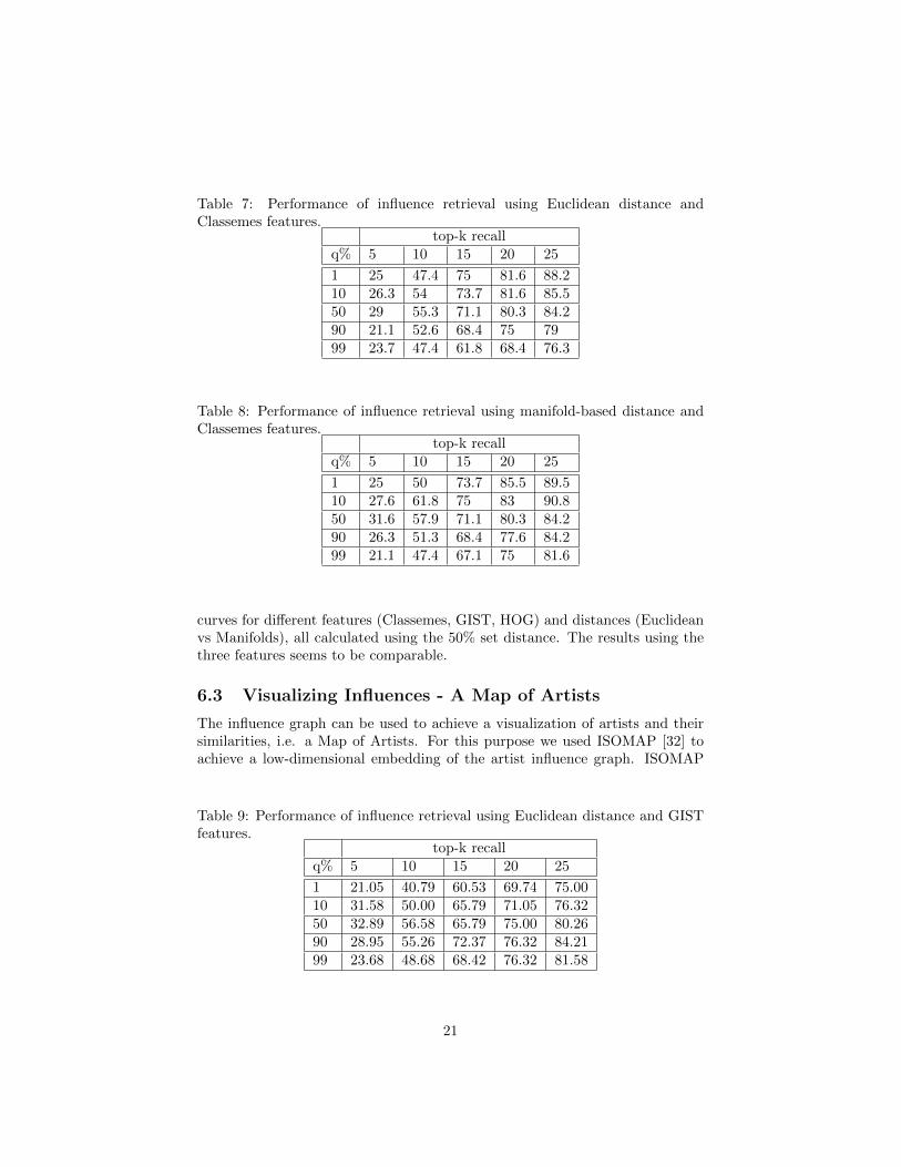
Table 7: Performance of influence retrieval using Euclidean distance andClassemes features.

top-k recallq% 5 10 15 20 25

1 25 47.4 75 81.6 88.210 26.3 54 73.7 81.6 85.550 29 55.3 71.1 80.3 84.290 21.1 52.6 68.4 75 7999 23.7 47.4 61.8 68.4 76.3

Table 8: Performance of influence retrieval using manifold-based distance andClassemes features.

top-k recallq% 5 10 15 20 25

1 25 50 73.7 85.5 89.510 27.6 61.8 75 83 90.850 31.6 57.9 71.1 80.3 84.290 26.3 51.3 68.4 77.6 84.299 21.1 47.4 67.1 75 81.6

curves for different features (Classemes, GIST, HOG) and distances (Euclideanvs Manifolds), all calculated using the 50% set distance. The results using thethree features seems to be comparable.

6.3 Visualizing Influences - A Map of Artists

The influence graph can be used to achieve a visualization of artists and theirsimilarities, i.e. a Map of Artists. For this purpose we used ISOMAP [32] toachieve a low-dimensional embedding of the artist influence graph. ISOMAP

Table 9: Performance of influence retrieval using Euclidean distance and GISTfeatures.

top-k recallq% 5 10 15 20 25

1 21.05 40.79 60.53 69.74 75.0010 31.58 50.00 65.79 71.05 76.3250 32.89 56.58 65.79 75.00 80.2690 28.95 55.26 72.37 76.32 84.2199 23.68 48.68 68.42 76.32 81.58

21

0  

10  

20  

30  

40  

50  

60  

70  

80  

90  

100  

5   10   15   20   25  

1  

10  

50  

90  

99  

0  

10  

20  

30  

40  

50  

60  

70  

80  

90  

100  

5   10   15   20   25  

1  

10  

50  

90  

99  

Figure 10: Influence recall curves, using classemes features with different q%.Left: Euclidean distance, Right: Manifold distance.

!"

#!"

$!"

%!"

&!"

'!"

(!"

)!"

*!"

+!"

,-'" ,-#!" ,-#'" ,-$!" ,-$'"

./011232145"

./011232146"

789:45"

789:46"

;<745"

;<746" !"

#!"

$!"

%!"

&!"

'!"

(!"

)!"

*!"

+!"

,-.//010/23"

,-.//010/24

"

567823"

567824"

9:523"

9:524"

;<'"

;<#!"

;<#'"

;<$!"

;<$'"

Figure 11: Influence Recall at different top-k: Comparisons of different descrip-tors

Table 10: Performance of influence retrieval using manifold-based distance andGIST features.

top-k recallq% 5 10 15 20 25

1 22.37 42.11 63.16 68.42 73.6810 34.21 53.95 67.11 69.74 78.9550 34.21 59.21 73.68 75.00 84.2190 30.26 55.26 71.05 73.68 78.9599 21.05 48.68 67.11 73.68 81.58

22

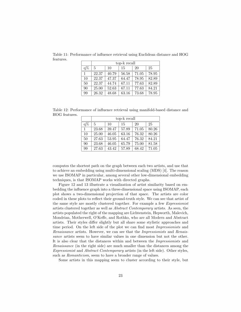
Table 11: Performance of influence retrieval using Euclidean distance and HOGfeatures.

top-k recallq% 5 10 15 20 25

1 22.37 40.79 56.58 71.05 78.9510 22.37 47.37 64.47 78.95 82.8950 22.37 44.74 67.11 77.63 82.8990 25.00 52.63 67.11 77.63 84.2199 26.32 48.68 63.16 73.68 78.95

Table 12: Performance of influence retrieval using manifold-based distance andHOG features.

top-k recall

q% 5 10 15 20 251 23.68 39.47 57.89 71.05 80.2610 25.00 46.05 63.16 76.32 80.2650 27.63 53.95 64.47 76.32 84.2190 23.68 46.05 65.79 75.00 81.5899 27.63 43.42 57.89 68.42 71.05

computes the shortest path on the graph between each two artists, and use thatto achieve an embedding using multi-dimensional scaling (MDS) [4]. The reasonwe use ISOMAP in particular, among several other low-dimensional embeddingtechniques, is that ISOMAP works with directed graphs.

Figure 12 and 13 illustrate a visualization of artist similarity based on em-bedding the influence graph into a three-dimensional space using ISOMAP, eachplot shows a two-dimensional projection of that space. The artists are colorcoded in these plots to reflect their ground-truth style. We can see that artist ofthe same style are mostly clustered together. For example a few Expressionistartists clustered together as well as Abstract Contemporary artists. As seen, theartists populated the right of the mapping are Lichtenstein, Hepworth, Malevich,Mondrian, Motherwell, O’Keffe, and Rothko, who are all Modern and Abstractartists. Their styles differ slightly but all share some stylistic approaches andtime period. On the left side of the plot we can find most Impressionists andRenaissance artists. However, we can see that the Impressionists and Renais-sance artists seem to have similar values in one dimension but not the other.It is also clear that the distances within and between the Impressionists andRenaissance (in the right side) are much smaller than the distances among theExpressionist and Abstract Contemporary artists (in the left side). Other styles,such as Romanticism, seem to have a broader range of values.

Some artists in this mapping seem to cluster according to their style, but

23

Figure 12: Map of Artists: Similar artists in two dimensions: Top: Dimensions1 and 2, Bottom: Dimensions 1 and 3. Artist are color coded by their style.

24

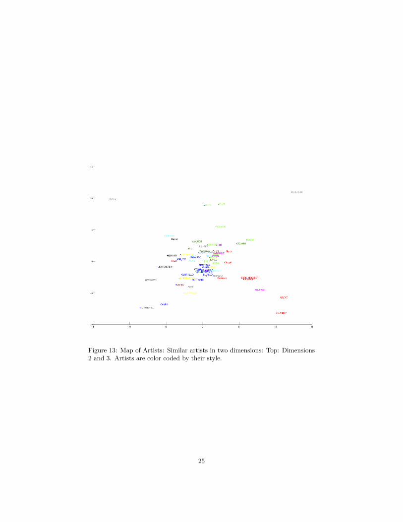
Figure 13: Map of Artists: Similar artists in two dimensions: Top: Dimensions2 and 3. Artists are color coded by their style.

25

in the context of influence, it is also important to think about the similaritiesbetween artists instead of the classification of style. This is yet another com-plication of the task of measuring influence. Therefore, another way to analyzethis graph is to disregard style all together. We can wonder whether Richterand Hockney share a connection because they lie close to each other. Or wecan wonder if Klimt was influenced by Picasso or Braque. In fact, both Picassoand Braque were listed as influences for Klimt in our ground-truth list. Whencomparing these close mappings to the ground truth influence, some are reason-able while others seem less coherent. In another example, Bazille lies close toDelacroix which is consistent with our ground truth. Other successful mappingsinclude Munch’s influence on Beckmann, Degas’s influence on Caillebotte, andothers. Figure 14 illustrates the top-5 suggested influence results.

7 Conclusion and Future Works

This paper scratches the surface of the problem of automated discovery of artistinfluence, through the study of painting and artist similarity. We posed theinteresting question of finding influence between painters as a knowledge dis-covery problem and showed interesting results for both of the qualitative andquantitative measurements.

In this paper we also studied the problem of paintings style classification,and presented a comparative study of three different models for the classificationtask, with different visual features. That study showed that semantic-levelfeatures perform the best for this task. This conclusion lead us to use thesesemantic features for the task of influence discovery.

For the task of influence discovery, we compared several distance measuresbetween paintings, including a Euclidean distance and a manifold-based dis-tance. The comparative experiments showed that the manifold-based distancegave slightly better results. We proposed and evaluated different artist distancemeasures, denoted as minimum-link, central-link, and maximum-link influencemeasures. This problem can be formulated as a set distance, however the typicalHausdorff set distance did not perform best, instead the central-link influencemeasure performed best in all experiments. We also present a tool for visualizingartist similarity through what we call a map of artists.

In this paper we also presented a new annotated dataset with diverse set ofartists and wide range of paintings. This dataset will be publicly available andcan be used for interdisciplinary tasks of Art and Computer Science.

Of course, there is a lot more to be done. For example, our framework couldinclude searching for specific stylistic similarities such as brushstroke and pat-tern. We could also include more features of color and line. We can experimentwith many other features especially among the elements and principles of art.Clearly there are many ways in which artists are influenced by each other. Thisis why mapping influence is such a difficult task.

26

Artist Influenced By:'BAZILLE' 'CEZANNE' 'RUBENS' 'DURER' 'DELACROIX' 'DEGAS''BELLINI' 'RAPHAEL' 'MANTEGNA' 'BOTTICELLI' 'VAN_EYCK' 'TITIAN''BLAKE' 'EL_GRECO' 'RAPHAEL' 'DURER' 'DELACROIX' 'VELAZQUEZ''BOTTICELLI' 'MANTEGNA' 'VAN_EYCK' 'MICHELANGELO''DURER' 'BELLINI''BRAQUE' 'Picasso' 'CEZANNE' 'RAPHAEL' 'JOHNS' 'MANTEGNA''Bacon' 'MANET' 'Beckmann' 'Picasso' 'VELAZQUEZ' 'RAPHAEL''Beckmann' 'Picasso' 'DURER' 'VELAZQUEZ' 'RAPHAEL' 'MICHELANGELO''CAILLEBOTTE''MANET' 'DELACROIX' 'CEZANNE' 'VAN_EYCK' 'DURER''CAMPIN' 'DONATELLO' [] [] [] []'CARAVAGGIO''RUBENS' 'TITIAN' 'EL_GRECO' 'LEONARDO' 'RAPHAEL''CEZANNE' 'Picasso' 'RENOIR' 'RUBENS' 'DELACROIX' 'EL_GRECO''Chagall' 'RAPHAEL' 'Picasso' 'Beckmann' 'MICHELANGELO''DELACROIX''DEGAS' 'CEZANNE' 'Picasso' 'RAPHAEL' 'DELACROIX' 'Munch''DELACROIX' 'RUBENS' 'EL_GRECO' 'RAPHAEL' 'DURER' 'TITIAN''DELAUNAY' 'MARC' 'Beckmann' 'MALEVICH' 'MACKE' 'CEZANNE''DONATELLO' 'MANTEGNA' 'VAN_EYCK' 'LEONARDO' 'BOTTICELLI' 'CAMPIN''DURER' 'LEONARDO' 'MANTEGNA' 'VAN_EYCK' 'RAPHAEL' 'TITIAN''EL_GRECO' 'RUBENS' 'TITIAN' 'DURER' 'RAPHAEL' 'MANTEGNA''GERICAULT' 'DELACROIX' 'TITIAN' 'RUBENS' 'GOYA' 'RAPHAEL''GHIBERTI' 'VAN_EYCK' 'DONATELLO' 'MANTEGNA' 'CAMPIN' []'GOYA' 'REMBRANDT' 'LEONARDO' 'DELACROIX' 'TITIAN' 'VELAZQUEZ''Gris' 'Picasso' 'Miro' 'BRAQUE' 'JOHNS' 'Munch''HEPWORTH' 'Picasso' 'Gris' 'JOHNS' 'Bacon' 'KLINE''HOCKNEY' 'RAPHAEL' 'MANET' 'rockwell' 'HOFMANN' 'Picasso''HOFMANN' 'MALEVICH' 'Munch' 'Klee' 'KLINE' 'MACKE''INGRES' 'TITIAN' 'LEONARDO' 'CARAVAGGIO''VELAZQUEZ' 'JOHNS''JOHNS' 'Picasso' 'BRAQUE' 'DURER' 'CEZANNE' 'RAPHAEL''KAHLO' 'CEZANNE' 'RAPHAEL' 'Picasso' 'RENOIR' 'LEONARDO''KANDINSKY' 'Chagall' 'BRAQUE' 'RAPHAEL' 'RUBENS' 'MICHELANGELO''KIRCHNER' 'EL_GRECO' 'Beckmann' 'Picasso' 'DELACROIX' 'MARC''KLIMT' 'VAN_EYCK' 'Picasso' 'JOHNS' 'Munch' 'MANTEGNA''KLINE' 'Beckmann' 'CAILLEBOTTE''MANET' 'INGRES' 'VELAZQUEZ''Klee' 'Picasso' 'CEZANNE' 'VERMEER' 'KLIMT' 'JOHNS''LEONARDO' 'DURER' 'RAPHAEL' 'VAN_EYCK' 'MANTEGNA' 'TITIAN''LICHTENSTEIN''Picasso' 'HOFMANN' 'Beckmann' 'RODIN' 'ROUSSEAU''MACKE' 'RAPHAEL' 'RUBENS' 'MARC' 'Picasso' 'CEZANNE''MALEVICH' 'Gris' 'Miro' 'Picasso' 'VELAZQUEZ' 'KAHLO''MANET' 'VELAZQUEZ' 'CEZANNE' 'RAPHAEL' 'Picasso' 'DEGAS''MANTEGNA' 'BOTTICELLI' 'VAN_EYCK' 'DURER' 'LEONARDO' 'MICHELANGELO''MARC' 'EL_GRECO' 'RAPHAEL' 'KIRCHNER' 'MICHELANGELO''Picasso''MICHELANGELO''RAPHAEL' 'DURER' 'TITIAN' 'MANTEGNA' 'LEONARDO''MONDRIAN' 'MALEVICH' 'BRAQUE' 'Picasso' 'KLIMT' 'JOHNS''MONET' 'PISSARRO' 'CEZANNE' 'SISLEY' 'VAN_GOGH' 'RENOIR''MORISOT' 'CEZANNE' 'RENOIR' 'DELACROIX' 'PISSARRO' 'MONET''MOTHERWELL''VELAZQUEZ' 'Beckmann' 'RODIN' 'Bacon' 'TITIAN''Miro' 'Picasso' 'Gris' 'JOHNS' 'VELAZQUEZ' 'ROUSSEAU''Munch' 'CEZANNE' 'Picasso' 'DURER' 'BRAQUE' 'MANTEGNA''Okeeffe' 'BRAQUE' 'MALEVICH' 'MONDRIAN' 'VAN_EYCK' 'MICHELANGELO''PISSARRO' 'CEZANNE' 'MONET' 'VAN_GOGH' 'RENOIR' 'SISLEY''Picasso' 'BRAQUE' 'CEZANNE' 'DURER' 'RAPHAEL' 'EL_GRECO''RAPHAEL' 'MICHELANGELO''DURER' 'MANTEGNA' 'TITIAN' 'LEONARDO''REMBRANDT' 'LEONARDO' 'TITIAN' 'VELAZQUEZ' 'DURER' 'EL_GRECO''RENOIR' 'CEZANNE' 'DEGAS' 'RUBENS' 'TITIAN' 'RAPHAEL''RICHTER' 'GOYA' 'RUBENS' 'TITIAN' 'RODIN' 'LEONARDO''RODIN' 'CEZANNE' 'VELAZQUEZ' 'DELACROIX' 'EL_GRECO' 'TITIAN''ROUSSEAU' 'VAN_GOGH' 'VAN_EYCK' 'BOTTICELLI' 'Picasso' 'DURER''RUBENS' 'TITIAN' 'EL_GRECO' 'RAPHAEL' 'VELAZQUEZ' 'DURER''Rothko' 'HOCKNEY' 'VELAZQUEZ' 'Picasso' 'Bacon' 'BRAQUE''SISLEY' 'PISSARRO' 'CEZANNE' 'MONET' 'RENOIR' 'VAN_GOGH''TITIAN' 'RAPHAEL' 'EL_GRECO' 'DURER' 'LEONARDO' 'BOTTICELLI''VAN_EYCK' 'DONATELLO' 'CAMPIN' [] [] []'VAN_GOGH' 'CEZANNE' 'MANTEGNA' 'DELACROIX' 'PISSARRO' 'DURER''VELAZQUEZ' 'EL_GRECO' 'RAPHAEL' 'LEONARDO' 'REMBRANDT' 'TITIAN''VERMEER' 'LEONARDO' 'VELAZQUEZ' 'VAN_EYCK' 'REMBRANDT' 'DURER''Warhol' 'Bacon' 'rockwell' 'Beckmann' 'LEONARDO' 'DEGAS''rockwell' 'Picasso' 'RAPHAEL' 'CEZANNE' 'DELACROIX' 'BRAQUE'

Figure 14: Top-5 suggested influences retrieved from the graph: using Classemesfeatures, Euclidean distance, and q=50%,

27

References

[1] A. E. Abdel-Hakim and A. A. Farag. Csift: A sift descriptor with color invariantcharacteristics. In IEEE Conference on Computer Vision and Pattern Recogni-tion, CVPR, 2006.

[2] Ravneet Singh Arora and Ahmed M. Elgammal. Towards automated classificationof fine-art painting style: A comparative study. In ICPR, 2012.

[3] Mikhail Belkin and Partha Niyogi. Laplacian eigenmaps for dimensionality re-duction and data representation. Neural Computation, 15:1373–1396, 2002.

[4] I. Borg and P.J.F. Groenen. Modern Multidimensional Scaling: Theory and Ap-plications. Springer, 2005.

[5] Christopher J. C. Burges. A tutorial on support vector machines for patternrecognition. Data Mining and Knowledge Discovery, 2:121–167, 1998.

[6] Ricardo S. Cabral, Joo P. Costeira, Fernando De la Torre, Alexandre Bernardino,and Gustavo Carneiro. Time and order estimation of paintings based on visualfeatures and expert priors. In SPIE Electronic Imaging, Computer Vision andImage Analysis of Art II, 2011.

[7] Gustavo Carneiro. Graph-based methods for the automatic annotation and re-trieval of art prints. In ICMR, 2011.

[8] Gustavo Carneiro, Nuno Pinho da Silva, Alessio Del Bue, and Joao PauloCosteira. Artistic image classification: An analysis on the printart database.In ECCV, 2012.

[9] Chih-Chung Chang and Chih-Jen Lin. LIBSVM: A library for support vectormachines. ACM Transactions on Intelligent Systems and Technology, 2:27:1–27:27, 2011.

[10] A. Ng D. Blei and M. Jordan. Latent dirichlet allocation. In Journalof MachineLearning Research, 2003.

[11] Navneet Dalal and Bill Triggs. Histograms of oriented gradients for human de-tection. In International Conference on Computer Vision & Pattern Recognition,volume 2, pages 886–893, June 2005.

[12] M-P Dubuisson and Anil K Jain. A modified hausdorff distance for object match-ing. In Pattern Recognition, 1994.

[13] Maria Vanrell Fahad Shahbaz Khan, Joost van de Weijer. Who painted thispainting? 2010.

[14] Li Fei-fei. A bayesian hierarchical model for learning natural scene categories. InIn CVPR, 2005.

[15] Lois Fichner-Rathus. Foundations of Art and Design. Clark Baxter.

[16] L.X. Fan J. Willamowski G. Csurka, C. Dance and C. Bray. Visual categorizationwith bags of keypoints. In Proc. of ECCV International Workshop on StatisticalLearning in Computer Vision, 2004.

[17] Friedenberg J. Rockmore D. Graham, D. Mapping the similarity space of paint-ings: image statistics and visual perception. Visual Cognition, 2010.

[18] Andrei Brasoveanu Shannon Hughes Ingrid Daubechies Gungor Polatkan, Sina Ja-farpour.

28

[19] Mark Harden. The artchive@http://artchive.com/cdrom.htm.

[20] W. Leow I. Widjaja and F. Wu. Identifying painters from color profiles of skinpatches in painting images. In ICIP, 2003.

[21] Alexei A. Efros Andrew Zisserman William T. Freeman Josef Sivic, Bryan C. Rus-sell. Discovering objects and their location in images. In ICCV, 2005.

[22] Theo Gevers Koen E. A. van de Sande and Cees G. M. Snoek. Evaluating colordescriptors for object and scene recognition. In IEEE Transactions on PatternAnalysis and Machine Intelligence, 2010.

[23] Jia Li, Lei Yao, Ella Hendriks, and James Z. Wang. Rhythmic brushstrokes dis-tinguish van gogh from his contemporaries: Findings via automated brushstrokeextraction. IEEE Trans. Pattern Anal. Mach. Intell., 2012.

[24] Thomas Edward Lombardi. The classification of style in fine-art painting. ETDCollection for Pace University. Paper AAI3189084., 2005.

[25] David G. Lowe. Distinctive image features from scale-invariant keypoints. Int. J.Comput. Vision, 2004.

[26] Andrew Y. Ng and Michael I. Jordan. On discriminative vs. generative classifiers:A comparison of logistic regression and naive bayes, 2001.

[27] Aude Oliva and Antonio Torralba. Modeling the shape of the scene: A holisticrepresentation of the spatial envelope. International Journal of Computer Vision,42:145–175, 2001.

[28] P. Kammerer R. Sablatnig and E. Zolda. Hierarchical classification of paintingsusing face- and brush stroke models. In ICPR, 1998.

[29] Robert Sablatnig, Paul Kammerer, and Ernestine Zolda. Structural analysis ofpaintings based on brush strokes. In Proc. of SPIE Scientific Detection of Fakeryin Art. SPIE, 1998.

[30] Fanhuai Shi, Xixia Huang, and Ye Duan. Robust harris-laplace detector by scalemultiplication. In ISVC (1) Lecture Notes in Computer Science.

[31] Josef Sivic and Andrew Zisserman. Efficient visual search of videos cast as textretrieval. IEEE Trans. Pattern Anal. Mach. Intell.

[32] J. B. Tenenbaum, V. Silva, and J. C. Langford. A Global Geometric Frameworkfor Nonlinear Dimensionality Reduction. Science, 290(5500):2319–2323, 2000.

[33] Roberto Toldo, Umberto Castellani, and Andrea Fusiello. A bag of words ap-proach for 3d object categorization. In Proceedings of the 4th International Con-ference on Computer Vision/Computer Graphics CollaborationTechniques, 2009.

[34] Lorenzo Torresani, Martin Szummer, and Andrew Fitzgibbon. Efficient objectcategory recognition using classemes. In ECCV, 2010.

[35] Theo van de Sande, Koen; Gevers and Cees G. M. Jan-Snoek. Evaluating colordescriptors for object and scene recognition. IEEE Transactions on Pattern Anal-ysis and Machine Intelligence, 32(9), 2010.

[36] Kilian Q Weinberger, Fei Sha, and Lawrence K Saul. Learning a kernel matrixfor nonlinear dimensionality reduction. In Proceedings of the twenty-first inter-national conference on Machine learning, page 106. ACM, 2004.

[37] Jun Yang, Yu-Gang Jiang, Alexander G. Hauptmann, and Chong-Wah Ngo. Eval-uating bag-of-visual-words representations in scene classification. In Proceedingsof the International Workshop on Workshop on Multimedia Information Retrieval,MIR ’07, 2007.

29