toward modeling and simulation of critical national ... · toward modeling and simulation of...
TRANSCRIPT

Toward Modeling and Simulation of Critical National Infrastructure
Interdependencies
Hyeung-Sik J. Min1, Walter E. Beyeler2, Theresa J. Brown3, Young Jun Son4,*, and Albert T.
Jones5
1Senior Member of Technical Staff, Sandia National Laboratories, Albuquerque, NM, USA, IIE
member grade if you have,
2Principal Member of Technical Staff, Sandia National Laboratories, Albuquerque, NM, USA,
3 Principal Member of Technical Staff, Sandia National Laboratories, Albuquerque, NM, USA,
4Assistant Professor, Systems and Industrial Engineering, University of Arizona, Tucson, AZ
85721-0020, USA; IIE Senior Member
5Manager, Enterprise Integration Program, Manufacturing Systems Integration Division, NIST,
Gaithersburg, MD 20899, USA, IIE member grade if you have
*Corresponding Author, Tel: 1-520-6269530, Fax: 1-520-6216555, E-mail: [email protected]
1
SAND2005-4828J

Toward Modeling and Simulation of Critical National Infrastructure
Interdependencies
Abstract
Modern society is dependent upon a complex network of interdependent critical infrastructures.
Continued prosperity and national security of the U.S. depend on our ability to understand and
analyze this complex network, and to timely and effectively respond to potential disruptions. In
this paper, we propose an innovative modeling and analysis framework for interdependent
critical infrastructures based on system dynamics, IDEF, and nonlinear optimization algorithms.
Collaborative efforts among Sandia, government agencies including DHS, commercial/private
industries, and academics have resulted in realistic models, including critical infrastructure
models, e.g. power, petroleum, natural gas, water, and communication, and economic sector
models, e.g. residence, industry, commercial sector, and transportation. The proposed
framework and models are demonstrated for hypothetical disruption of a critical infrastructure
and optimal response.
1. Introduction
The continued prosperity and national security of the U.S. is dependent on reliable
operation of the complex network of interdependent, large-scale critical infrastructures. The
impact of capacity excess or disruptions of them on defense and economic security of the nation
would be devastating. Therefore, our ability to model and analyze them is of critical importance
2
to timely and effectively respond to potential disruptions. Although efforts to understand the
interdependences of the critical infrastructures have taken on increasing importance during the
last decade, it was learned that modeling and analysis of them is an extremely difficult task. This
is because 1) data acquisition is difficult, 2) each individual infrastructure itself is very
complicated, 3) infrastructures evolve and the regulations governing their operation change, and
4) it is impossible to construct a realistic model without a leading role of a government agency
coordinating commercial/private industries.
More recently, Sandia National Laboratories have collaborated with government
institutions, industries, and academics to understand the potential consequences of infrastructure
interdependencies. The goal of the program is to develop modeling and analysis tools for
evaluating potential effects of disruptions of critical infrastructures and mitigating them under
collaboration with other national laboratories and industries, and government institutions. In this
paper, we first discuss an innovative modeling framework for simulation and decision support
system of interdependent critical infrastructures based on system dynamics, IDEF, and nonlinear
optimization algorithms. We then provide examples of how we apply them in a certain
disruption scenario, where the key task is to allocate scarce resource of critical infrastructures.
The remaining sections are organized as follows. In Section 2, we discuss definitions,
scope, and issues of critical infrastructures. In Section 3, the overview of methodologies used in
this research is discussed. The modelling framework and experimental results with model are
then presented in Section 4. Finally, conclusions are drawn in Section 5.
2. Interdependencies of Critical Infrastructures and Their Protection
3
U.S. Critical Infrastructure Assurance Office defines an infrastructure as “the framework
of interdependent networks and systems comprising identifiable industries, institutions
(including people and procedures), and distribution capabilities that provide a reliable flow of
products and services and services essential to the defense and economic security of the U.S., the
smooth functioning of governments at all levels, and society as a whole” (Presidential Decision
Directive 63). In this perspective, infrastructures include agriculture/food, drinking water,
banking and financing, chemical industry and hazardous materials, defense industrial base,
public health, emergency services, energy, government, information and telecommunication, and
postal and shipping. More recently after the 911 terror attack, other key assets have been added
into the consideration including national monuments and icons, nuclear power plants, dams,
government facilities, and commercial key assets.
Critical infrastructure protection means not only protecting infrastructure itself but also
protecting the services, physical and information flows, role and function and specially
symbolized core values of the infrastructures. Criticality of the infrastructures can be either
teleological or systematic. Teleological criticality means that an infrastructure is inherently
critical, because of its role or function in society. An existential security policy objective can no
longer be achieved in the event of the collapse of, or damage to the infrastructure. For example,
the U.S. Congress and Whitehouse are attractive targets, not because they are connected in some
way, but they are symbols of national power. On the other hand, systematic criticality means
that an infrastructure is critical because of its structural positioning in the whole system of
infrastructures and it is an important link between other infrastructures or sectors (Metzger,
2004).
4
In the real world, no infrastructure stands alone. If electric power distribution is
disrupted and power goes off, then traffic lights go off and phone and email systems go off.
Thus the electric power, transportation and communication infrastructures are linked and
interdependent. Deliberate attacks or serious accidental system failures of one infrastructure
may result in serious consequences to the nation because of the interrelationship among
infrastructures and its potential cascading effects. Some of the infrastructures have the potential
to impact many other infrastructures. Electric power and telecommunications influence the
operational capacity or demand side for almost all of the other infrastructures, while all the
infrastructures and demand sectors interact with and through the banking and finance system.
Other infrastructures and sectors such as chemicals and hazardous materials, defense industrial
base and key national resources tend to be impacted by infrastructure disruptions but do not tend
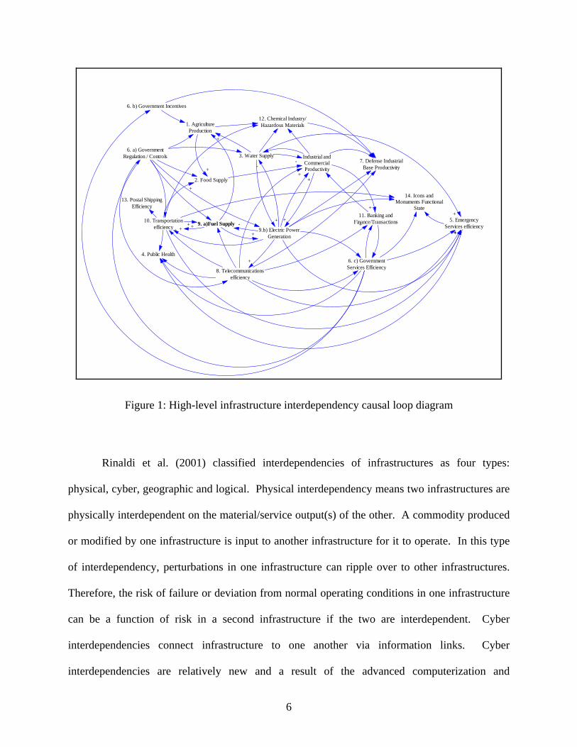
to propagate the effects to other infrastructures or regions. The degree of connectivity through
potential major interactions between each of the infrastructures is illustrated using a causal loop
diagram (CLD) in Figure 1. The variables, which directly influence each other, are connected by
directional arrows with a ‘+’ or ‘−’ sign. The sign ‘+’ means that changes in the first variable
cause changes in the same direction in the second variable; the sign ‘−’ means that the first
variable causes a change in the opposite direction in the second variable. The behavior of the
entire infrastructure system is the result of the complex interrelationships among the various
system variables. While the causal loop diagram depicts a high-level interdependency among
variables, system dynamic (SD) models (see Figure 3) contain explicit equations (differential or
difference equations) governing their relationships.
5
6. c) GovernmentServices Efficiency
Industrial andCommercialProductivity
9.b) Electric PowerGeneration
3. Water Supply
9. a)Fuel Supply
1. AgricultureProduction
8. Telecommunicationsefficiency
10. Transportationefficiency
5. EmergencyServices efficiency
6. a) GovernmentRegulation / Controls
+
-
+
+
-
+
+
+ + ++
+
+++
--
+2. Food Supply
+ +
+
11. Banking andFinance/Transactions
+
+
+
6. b) Government Incentives
7. Defense IndustrialBase Productivity
13. Postal ShippingEfficiency
4. Public Health
14. Icons andMonuments Functional
State
12. Chemical Industry/Hazardous Materials
Figure 1: High-level infrastructure interdependency causal loop diagram
Rinaldi et al. (2001) classified interdependencies of infrastructures as four types:
physical, cyber, geographic and logical. Physical interdependency means two infrastructures are
physically interdependent on the material/service output(s) of the other. A commodity produced
or modified by one infrastructure is input to another infrastructure for it to operate. In this type
of interdependency, perturbations in one infrastructure can ripple over to other infrastructures.
Therefore, the risk of failure or deviation from normal operating conditions in one infrastructure
can be a function of risk in a second infrastructure if the two are interdependent. Cyber
interdependencies connect infrastructure to one another via information links. Cyber
interdependencies are relatively new and a result of the advanced computerization and
6

automation of infrastructures. The outputs of the information infrastructure are inputs to the
other infrastructure, and the commodity passed between the infrastructures is information. The
breakage of this information link between infrastructures may cause the physical flow of
material/services between them. Geographical interdependency means that more than two
infrastructures can be geographically interdependent based on their physical proximity. Events
such as explosion or fires could create correlated disturbances in these geographical
interdependent infrastructures. However, the state of one infrastructure dose not effect on the
state of another. Logical interdependency means that two infrastructures are logically
interdependent if the state of each depends on the state of others via human decisions and
actions. For example, gas price low it results in increased traffic congestion. In this case, the
logical interdependency between the petroleum and transportation infrastructures is due to
human decisions and actions and is not the result of a physical process.
Modeling and analysis of critical infrastructures interdependencies are complex and
challenging tasks for several reasons. First, the majority of the infrastructure is owned by
commercial or semi-commercial interests, and acquisition of data and information is difficult.
Private infrastructure owners should operate competitively using their limited capital investments
and operational expenses. Safety and security of infrastructure components beyond what is
required by regulatory authority and legal requirements are not their primary concerns compared
to providing an immediate competitive advantage. Sharing or exchange of information required
to maintain either interdependent elements of infrastructure or the entire infrastructure can put
the civilian infrastructure owners at a disadvantage. This can occur when required information
sharing in a given sector exposes business intelligence (e.g. cost structure, process capacities) to
the competitors in the same or another sector. Therefore, the data and information collected and
7

exchanged in the interest of improving the robustness, availability, and overall assurance of
infrastructure elements must be protected against malicious interests and influence (Wolthusen,
2004). In this work, Sandia has collaborated with Department of Homeland Security, other
national laboratories, and commercial/private industries to develop realistic models. To the best
of our knowledge, the models addressed in this paper are among the most comprehensive critical
national infrastructure ones. Second, many models and computer simulations exist for aspects of
individual infrastructures such as electric power networks model, traffic management models for
transportation network, telephone call traffic analysis models, among others. However, simply
hooking several existing infrastructures does not work; every model has its unique assumptions,
data, and numerical requirements (e.g. time units, scaling limits or computational algorithms)
that may not be compatible with other models. Further, such approaches do not capture
emergent behavior, or a key element of interdependency analysis. Therefore, it requires more
intensive studies of integration aspects of individual critical infrastructures such as matching
time resolutions and data conversion and mapping between two critical infrastructure models
based on time-step or requirements. In this work, IDEF∅ model (see Section 4) of the critical
infrastructure has been developed to form a basis for the integration of individual infrastructure
models. Last, each individual critical infrastructure has its own objective function such as
minimizing communication traffics for communication infrastructures and promising secure
transactions for banking and financing infrastructures. Some of objective functions of individual
critical infrastructure might have conflicts, and could not be satisfied simultaneously. No single
approach will address and meet all the different objectives of different critical infrastructures.
Therefore, some ultimate global objective function, which is agreed with all critical
infrastructure owners and users, has to be determined. In this work, we have developed a global
8
objective function from the perspective of a governmental mediator to minimize the impact on
the whole society in the case of disruptions.
3. Overview of Methodologies
This section discusses an overview of three major methodologies used in this research for
integrative modeling and analysis of interdependent infrastructures. They are system dynamics,
IDEF system specification tool, and nonlinear optimization algorithms.
System dynamics (SD) is a method of for studying the dynamics of the real-world
systems around us. Its key concept is that all the objects in a system interact through causal
relationships. Three core factors that constitute a SD model include (Reid and Koljonen 1999):
1) the structure of the system, expressed in the form of feedback-based causal loop diagrams, 2)
the frequency and duration of time delays in the feedback loops, and 3) the amplification of the
information flows through the feedback structure. Simulations based on these factors can
provide insight into important causes and effects, which can lead to a better understanding of the
dynamic and evolutionary behavior of the system as a whole. They can yield a time-based plan
based on a dynamic view of the system rather than a fixed plan based on static view of the
system.
The causal loop diagram (see Figure 1), an abstract SD model, does not capture the stock
an flow structure of the system (Richardson 1986, Richardson 1997, Sterman 2000, Binder et al.
2004), which is required to model the dynamic system exactly and derive the appropriate
differential equations. Such a model can however be modeled as Stock and Flow Diagrams (see
Figure 3; Sterman 2000), a more detailed SD model. System dynamics is particularly
appropriate to model complex overall interactions for which very sparse data (if any) are
9

available. In addition, it can take randomness into account and enables a form of
experimentation not possible in the real systems. Finally, it enables to gain insight into the
stability of the system via transformation to the closed loop transfer functions (Disney and
Towill 2002). However, explicit stability analysis is beyond the scope of this paper.
A formal system modelling technique has been employed to describe the proposed
interdependency SD simulation model of the critical infrastructures and economic sectors. The
purpose of a system model is to help define data requirements and describe the exchange of
information between models. It lays down unambiguous guidelines that facilitates the
development of a large scale, networked, computer environment that behaves consistently and
correctly. In this work, functional modelling (IDEF∅, see Figure 4), a system description
technique developed by the U.S. Air Force, is used to identify the system functions within the
system, along with the flow of information and objects which relate the functions. The
hierarchical nature of IDEF∅, the primary strength of the method, facilitates the ability to
construct models that have a top-down representation and interpretation, but which are based on
a bottom-up analysis process. Beginning with raw data, the modeller starts grouping together
functions that are closely related or functionally similar. Through this grouping process, the
hierarchy emerges (http://www.idef.com/ at KBSI). Modelling efforts in this research consider
over 5000 variables and parameters, and therefore, we benefit from the hierarchical nature of
IDEF significantly. As mentioned earlier, IDEF∅ model (see Section X) of the critical
infrastructure has formed a basis to integrate individual infrastructure SD models in this work.
Once the integrative SD model of the critical infrastructure is constructed, we need to
find the values for the input variables such that an expected system performance from the SD
simulation is optimized. In this work, the objective function is to maximize total economic
10

revenue in the case of disruptions (see Section 3.1). Contemporary simulation optimization
methods (Azadivar and Tompkins 1999) include (1) gradient-based search methods, (2)
stochastic approximation methods, (3) sample path optimization, (4) response surface methods,
and (5) meta-heuristic search method, including genetic algorithms, simulated annealing, and
tabu search. In this work, we employ a suite of nonlinear optimization algorithms, which is
combined into MINOS software package (Murtagh and Sanders 1998), since it is widely known
and available. In MINOS, problems with linear constrains and nonlinear objectives are solved
using a reduced-gradient algorithm (Wolfe 1962) in conjunction with a quasi-Newton algorithm
(Davidon 1959). On the other hand, those problems containing nonlinear constraints are solved a
projected augmented Lagrangian algorithm, based on a method due to Robinson (1972). To
overcome the problems of local optimum, we start the optimizer in a number of different places.
Performance investigation of different optimization approaches is important but is beyond the
scope of this paper.
4. Interdependency Model of Critical Infrastructures and Optimization Problem
The integrative interdependency model of critical infrastructures simulates the effects of
loss in capacity of an infrastructure on other infrastructures and economic sectors. Each
infrastructure model includes the available capacity for the supply side of the system (production
and transportation process) as a function of the maximum production capacity and reductions in
that capacity due to damage of physical system or shortages of essential inputs (dependencies on
other infrastructure services). The simulations are driven by historical demand time series that
account for diurnal and seasonal variations in demand. Prices are modeled as a function of the
ratio of supply to demand and demand elasticity functions that alter the demand in response to
11

price. In this section, we provide details of modeling critical infrastructure interdependencies
using system dynamic simulation techniques.
4.1. Problem Definition and Model Description
In this study, the proposed interdependency simulation model of critical infrastructures
will provide the capability to allocate the available infrastructure services or materials to each of
other infrastructures and to economic sectors in order to minimize potential economic impacts of
the given scenarios with various magnitude, extent, and duration of disruptions on an
infrastructure. The notation used in the proposed model is shown below:
Notation:
Li = capacity loss of critical infrastructure i;
CIi = total available products/services of critical infrastructure i;
αij = satisfaction rate of desired consumption of Product/Service i for demand sector j;
Dij = desired consumption of product/service i for demand sector j;
Iij = available inventory of product/service i for demand sector j;
ERj = economic revenues of demand sector j
Rij = relative availability of product/Service i for sector j;
LA = labor availability;
APij = allocated product/service i for demand sector j;
i = p(Power), f(Fuel), g(Natural Gas), w(Drinking Water), c(Communication);
j = R(Residential), C(Commercial), I(Industrial), T(Transportation).
12

Our objective function is to find optimal αij to maximize total economic revenue TER = ∑ ERi,
while the disruption of a certain infrastructure i. Economic revenue ERi is the cumulative
difference between income Ii and expenditures Si in sector i over the model period [0, T]:
( dtSIERT
iii ∫ −=0
) (1)
Residential sector income is from wages, while income in the remaining sectors arises from
output purchased by other sectors. Expenditures are divided into purchases of generic goods and
services from other sectors, and purchase of infrastructure services such as electric power and
fuel. Infrastructure service purchases are distinguished from generic commercial and industrial
output because the specific technical factors influencing production and consumption are the
focus of the model. No distinction is made between capital purchases (investment) and operating
expenses in the commercial and industrial sectors. Purchasing rate for both generic goods and
infrastructure output is a function of a normalized performance indicator X , which measures the
current performance of each sector relative to its optimal value:
( )XfS = (2)
A portion of the generic purchases made by each sector are assumed to be non-deferrable, in that
if operational disruptions interfere with their timely execution they will not be reattempted later.
Other purchases may be reattempted. The “function” f( ) is in general non-linear and path-
dependent, and is specified by the dynamic model of the sector.
Figure 2 shows the sequence diagram to find optimal αPj when the power infrastructure
has the loss of power generation capacity Lp. The required procedures to find the solutions are as
follows:
13

• Step 1: Detect the loss of power generation capacity Lp due to the disruption or damage of
power infrastructure. For example, Lp = 0.3 means that 30% of power generation
capacity is lost.
• Step 2: Calculate available power production after the disruption, CIP
• Step 3: Choose αpj (0 ≤ αPj ≤ 1), provide allocated power, αPj * DPj (j = R, C, I, T) to each
economic Sector j. Here, ∑= PjPjP DCI α .
• Step 4: Calculate RpI, RpC, RpT and LA from economic sector simulators. Relative
available power Rpj is presented as a value from zero to one. One means the sector has
enough power to fully satisfy corresponding power requests of other industry related
infrastructures (e.g. petroleum and natural gas in our study). Its calculation includes the
inventory, the own power generation and battery or alternative power sources of the
economic sector. For example, RpI = 0.8 means that the industry economic sector only
has the power to satisfy 80% of industry power requests. RpI = 0.8 is input to the
corresponding infrastructure sub-system (petroleum and natural gas in our study).
However, residential sector only provides the work forces to all infrastructures. It is also
presented as a value from zero to one for available labors. Insufficient power supply to
residential sector will decrease the labor availability not directly but indirectly with such
as spending more time for commuting and house works.
• Step 5: Using given RpI, RpC, RpT and LA, determine each availability of critical
infrastructure materials/services CIi (I = f, g, w, c) and distribute them to economic sector
simulators with using each material/service market allocation algorithm.
• Step 6: Calculate Total economic Revenues, TER = ∑ ERi (i = R, C, I, T)
• Step 7: Change αpj and repeat step 3 to step 6 until finding the optimal TER.
14

Power Petroleum Natural Gas Water Communic
ation
Integrated Critical Infrastructure Model
DSSResidence Industry Commercial
Sector Transportat
ion
Integrated Economic Sector Model
Power Disruption
Lp
Available power after disruption, CIP
Relative Available Power for each sector
Available Labor, LARpI
RpC
RpT
Choose αpj(0 ≤ αPj ≤ 1)
αpR*DpR
αpI*DpI
αpC*DpC
αpT*DpT
Allocated Powers
Desired Power Consumption for each sectorDpI
DpC
DpT
DpR
Available Fuel, CIf
Available Natural Gas, CIg
Available Water, CIw
Available Communication, CIc
Economic Revenues for Each SectorERI
ERC
ERT
ERR
Max. TER= ∑ ERi ? Stop
YesNo
Iteration
Allocations are done automatically, using Market Allocation Algorithms
text
Figure 2: The sequence diagram of power disruption scenario
In this study, we have two allocation algorithms which include market allocation
algorithm and simulation based non linear optimization algorithms. The market allocation
algorithm uses supply curves specified for each infrastructure service provider, and demand
curves defined for each sector, to determine a market-clearing price for each service. The supply
curve for a particular infrastructure service may be compounded from different supply curves for
different types of provider within each infrastructure service model. The supply curve for
electric power, for example, is composed of supply curves for distinct generator classes (based
on fuel type) as well as supply curves characterizing the willingness of connected regions to
15

export power. Demand curves are generally specified to be horizontal, so that infrastructure
customers are price takers. The specification of inelastic demand reflects the assumption that
customers will be unable to significantly change their process or technology over the time frame
of the simulation. However, market allocation algorithm does not consider either markets of the
other infrastructures materials or services, or national economical impacts. Without the any
disruption of critical infrastructures, we assume that allocation of each infrastructure
services/materials is determined by its market allocation algorithm. However, when we have a
disruption of certain infrastructure and cause the shortage of service/materials of the disrupted
infrastructure, the government or other federal institutions could intervene the market of the
disrupted critical infrastructure, in order to satisfy or meet the global goal, which is finding the
maximum national economic revenue during a certain satiation. In this study, the decision
support system (DSS) finds the best strategy for allocation of insufficient materials/services of
the disrupted infrastructure using simulation based non linear optimization algorithm.
As shown in Figure 2, our model divides to three major parts including integrated critical
infrastructure model, decision support system (DSS), and integrated economic sector model.
Integrated critical infrastructure model merged five individual critical infrastructure models
which include power, petroleum, natural gas, drinking water and communication infrastructures.
Each individual infrastructure model is built as the supply chain system of materials/services of
an infrastructure using system dynamics modeling techniques. Each model is represented by an
aggregate inventories and flows of materials/services of an infrastructure at an appropriate
regional scale. For example, Figure 4 shows the power generation component of power
infrastructure system dynamics model, which presents that state level aggregates of power
demand drive the regional power generation rates with imports used to bring in cheaper power or
16

offset regional power shortfalls. In addition, each model is a stand-alone model prior to being
merged into the integrated model. This allows individual model elements to be tested and
utilized without the necessity or complexity of running the entire national interdependency
model. Most of the demand for infrastructure services are not determined by other
infrastructures, but by the economic sectors. The economic sector demand is aggregated at the
regional level of for residential, commercial and industrial sectors of consumers. In this study,
integrated economic sector demand model consists of four economic sector modules which are
Residence, Industry, Commercial and Transportation. The role of these sector models is to
define demands for the materials and services supplied by the basic infrastructures, capture the
broader economic consequences of disruptions to those materials and services, and represent the
interactions among those sectors to the extent that impaired performance in one sector, arising
from infrastructure disruptions, may influence the economic activities and infrastructure
demands in the other sectors. Finally, DSS includes the mechanism to find the allocation
parameters using simulation based non linear search algorithm.
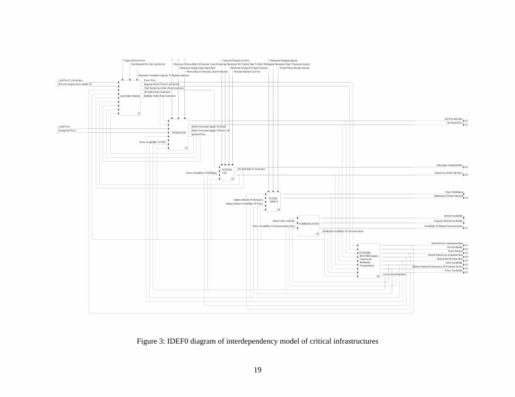
Figure 3 shows the IDEF∅ diagram for the high level view of the proposed
interdependency simulation model of critical infrastructures and economic sectors. As
mentioned earlier, more than 5000 variables and parameters have been considered in the entire
integrated model in this research. Therefore, we have benefited from the hierarchical
presentation and decomposition capability of IDEF∅. In the diagram, the rectangular box
represents the functions and the arrows represent the information an object flow. Arrows
entering on the left side of the box are the inputs to the function; arrows entering the top of the
box are the control on the function; arrows entering the bottom of the box are the mechanisms
that perform the function; and the arrows leaving the box on the right side are the outputs of the
17
18
function. Each function is associated with a unique ID number. Each function can be
decomposed into detailed sub-functions as much as detail. The diagram shows the relationship
among infrastructures and economic sectors, and also defines the variables which connect or
interface among them.
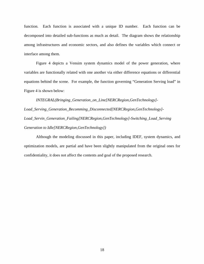
Figure 4 depicts a Vensim system dynamics model of the power generation, where
variables are functionally related with one another via either difference equations or differential
equations behind the scene. For example, the function governing “Generation Serving load” in
Figure 4 is shown below:
INTEGRAL(Bringing_Generation_on_Line[NERCRegion,GenTechnology]-
Load_Serving_Generation_Becomming_Disconnected[NERCRegion,GenTechnology]-
Load_Servin_Generation_Failing[NERCRegion,GenTechnology]-Switching_Load_Serving
Generation to Idle[NERCRegion,GenTechnology])
Although the modeling discussed in this paper, including IDEF, system dynamics, and
optimization models, are partial and have been slightly manipulated from the original ones for
confidentiality, it does not affect the contents and goal of the proposed research.
O1
O8O1
O1O2
O3
O1
O9O5O6O1
O4
O7
O1
ECONOMIC SECTORS (Industry , Commercial, Residential, Transportation)
A6
COMMUNICATION
A5
WATER SUPPLY
A4
NATURAL GAS
A3
PETROLEUM
A2
ELECTRIC POWER
A1
Current Total Population
Desired Fuel Purchase Rate
Desired Power Consumption Rate
Desired Natural Gas Acquisition Rate
Relative National Performances Of Economic Sectors
Water Demand
Power Availability
Labor Availability
Fuel Availability
Residential Availability Of Communications
Availability Of Business Communications
Internet Availability
Corporate Network AvailabilityRepair Labor Available
Power Availability To Communication Zones
Satisfaction Of Water DemandWater Distribution
Industry Relative Availability Of PowerIndustry Relative Performance
NG Sales Rate To GeneratorsNatural Gas Whole Sale Price
Natural gas Acquisition Rate
Power Availability In NGRegion
Crude PriceForeign Fuel Price
District Generators Supply Of DieselDistrict Generators Supply Of Heavy OilSpot Fuel Price
Fuel Purchase RateFuel Retail Price
Power Availability To PAD
Power PriceRegional Electric Power Load Served
Distillate Orders From GeneratorsOil Orders From GeneratorsTotal Natural Gas Orders From Generators
Coal Price To GeneratorsPrice For Imports From Outside US
Maximum Pumping CapacityMaximum Water Treatment Capacity
Treated Water Storage Capacity
Expected Natural Gas PriceMaximum NG Transfer Rate To Other NGRegions
Maximum Foreign NG Import CapacityNominal National Gas Price
Maximum Deliverability Of Domestic Crude ProductionMaximum Foreign Crude Import Rate
Normal Rate Of Domestic Crude Production
Expected Power PriceFuel Required Per Unit Load Served
Maximum Translation Capacity To Regions Customers
Figure 3: IDEF0 diagram of interdependency model of critical infrastructures
19

Idle PowerGenerationCapacity
FailedGenerationCapacity
Repairing Failed GenerationCapacity
Failed GenerationCapacity Repair Time
Fuel Required forServing Load
Time to ActivateGeneration
<TIME STEP>
Bringing Generationon Line
GenerationServing Load
Switching LoadServing
Generation toIdle
Load ServingGeneration Failing
GenerationFailure Time
Maximum Rate ofIncreasing Load Serving
AvailableGeneration
Net Rate of IncreasingLoad Serving
GenerationDisconnected
fromTransmission
SystemLoad Serving GenerationBecomming Disconnected
Idle GenerationBecomming
Disconnected
GenerationBecomming
Reconnected
GenerationReconnection Time
GenerationDisconnection RateInterruption
Start Time
InterruptionDuration
Disconnection RateDuring Interruption
<Time>
Emissions per UnitGeneration
Emissions Rate
Reserve Margin
Total IdleCapacity
Total GenerationServing Load
Effect of Power SCADAon Control of Generators
<Effect ofCommunications onPower SCADA>
<Relative GenerationCapacity without
SCADA>
Total AvailableGeneration
Maximum ControllableGeneration
Initial GenerationCapacity
Disconnection Rate dueto Control Limitations
<TIME STEP>
Idle capacity includes ancillaryservices. Current model does notinclude fuel used in providing these
services
Figure 4: Power generation system dynamics model
4.2. Preliminary Experiments and Results
In this work, we have conducted a preliminary experiment based on three scenarios with
the proposed models. Simulation start time is time 0 hour and all the parameters are initialized
based on the historical data which are collected from both various government agencies and
private industries. The time step ∆t of system dynamics simulation is 0.25 hour, and the run
length of the simulation is 108 hours. In Scenario 1, we run the base scenario without
considering a disruption of any critical infrastructure. In Scenario 2, we have a power disruption
20

starting at time 60 hour and ending at time 108 hour. The loss of power generation capacity
during the disruption is Lp = 0.4, which means 40% of power generation capacity is lost at time
60 hour. The allocation of power is determined by the decision support system using simulation
based nonlinear optimization algorithm, and allocation of other infrastructure materials/services
is determined by the market allocation of each critical infrastructure. In Scenario 3, we use the
same conditions with Scenario 2 except that the market allocation algorithm of each critical
infrastructure determined the allocation of each infrastructure materials/services. There is no
intervention to markets of infrastructures materials/services by the government or other
authorities.
Figure 5 depicts the comparison of the change of total revenue, ∆(∑ERi), over simulation
run for three scenarios. The result reveals “Scenario 2” outperforms “Scenario 3” in terms of the
change of total economic revenues. After the disruption occurred at time 60 hour, the change of
total revenue, ∆(∑ERi) of Scenario 2 is always higher than that of Scenario 3. In addition, the
cumulative total economic revenues of three scenarios during the disruption periods (from time
60 to time 108) are $1106M, $940M, and $603M, respectively. In terms of the cumulative total
economic revenues during the disruption period, DSS (Scenario 2) outperforms the market
algorithm of power (Scenario 3) by 15.6%. Therefore, based on the results of the experiment,
the intervention of market of the critical infrastructure may be necessary in the case of
disruptions or damages in order to minimize global economic impact.
21

The Change of Total Economic Revenues
12 24 36 48 60Time (Hour)
72 84 96 1080
3
33
3
3 3
3
3
1
1 1
1 1
1
1
2
2 2
2
2
2
2 2
2
22
2 2
2 2
1333333
1
1
11
11
1
1
1
800
600
400
200
0
scenario 3 M$/Day1 1 1 1 1 1 1 1 1
scenario 2 scenario 1
M$/Day2 2 2 2 2 2 2 2 2 M$/Day3 33333 3 333
Figure 5: Comparison of results of scenarios
5. Conclusion and future works
The proposed interdependency simulation model of critical infrastructures determines (1)
the availability of infrastructure services or materials to each of other infrastructures and to
economic sectors for given specific scenarios of damage or disruption to a certain infrastructure,
and (2) estimate the potential global economic effects of the given disruption with certain
magnitude, extent, duration of disruptions on a infrastructure.
For the future work, each infrastructure model is very aggregated level so it might be
good to be communicated with detailed simulation models of industrial manufacturing
companies or communication and transportation network models. It will help decision-makers to
test whether the policies from higher level is also feasible in lower level. In addition, it will be
nice that the change of variables and parameters in lower level detailed simulator is updated to
22

the variables and parameters of higher level simulators in a real time fashion, in order to provide
the accurate information to higher level decision-making process.
Acknowledgement
- By Theresa Brown
Product Disclaimer
Commercial software products are identified in this paper. These products were used for
demonstrations purpose only. This does not imply approval or endorsement by both Sandia
National Laboratory and NIST nor that these products are not necessarily the best available for
the purpose.
References
Azadivar, F., and Tompkins, G., (1999) Simulation optimization with qualitative and structural
model changes: A genetic algorithm approach, European Journal of Operational Research, 113,
169-182.
Binder, T., Vox, A., Belyazid, S., Haraldsson, Hordur, and Svensson, M., (19XX) Developing
system dynamics models from causal loop diagrams, XXXX.
Brown T., Beyeler, W., and Barton D., (2004) Assessing Infrastructure Interdependencies: The
Challenge of Risk Analysis for Complex Adaptive Systems, International Journal of Critical
Infrastructures, vol. 1, No. 1, pp. 108 – 117.
23

Davidon, W.C., (1959) Variable metric methods for minimization, A.E.C. Research and
Development Report ANL-5990, Argonne National Laboratory, Argonne, Illinois.
DeDomenico, C., Diersen S., Mintz, L., Tilson W., Haimes, Y. and Lambert, J., (2000)
Department of Defense Risk Management Model: New Methodologies For Infrastructure
Protection, 2000 System Engineering Capstone Conference – University of Virginia.
Disney, S.M. and Towill, D.R., (2002) A procedure for the optimization of the dynamic response
of a Vendor Managed Inventory system, Computers & Industrial Engineering, 43, 27-58.
Dudenhoeffer, D., Permann, M. and Sussman, E., (2002) A Parallel Simulation Framework for
Infrastructure Modeling and Analysis, Proceedings of the 2002 Winter Simulation Conference,
1971 – 1977.
Murtagh, B., and Saunders, M., (1998) MINOS 5.5 User’s Guide, Technical Report SOL 83-
20R, Stanford University.
Metzger, J., (2004) An Overview of Critical Infrastructure Protection: A Critical Appraisal of a
Concept, Workshops – Cyber Security 2004, Zurich, Switzerland.
The White House, (2003) National Strategy for the Physical Protection of Critical Infrastructures
and key Assets, pp 4-6, http://www.whitehouse .gov/pcipb/physical.html.
24
Rabelo, L., Helal, M., Jones, A., Min. J., Son, Y.-J., and Deshmukh, A., (2003) A Hybrid
Approach to Manufacturing Enterprise Simulation, Proceedings of the 2003 Winter Simulation
Conference, New Orleans, LA.
Reid, R. A. and Koljonen, E. L., (1999) Validating a manufacturing paradigm: a system
dynamics modeling approach. Proceedings of the 1999 Winter Simulation Conference (Phoenix,
AZ), 759–765.
Richardson, G., (1986) Problems with causal-loop diagrams, Systems Dynamics Review, vol. 2,
No. 2, pp. 158 – 170.
Richardson, G., (1997) Problems in causal loop diagrams revisited, Systems Dynamics Review,
vol. 13, No. 3, pp. 247 – 252.
Rinaldi, S., Peerenboom, J. and Kelly, T., (2001) Identifying, Understanding, and Analyzing
Critical Infrastructure Interdependencies, IEEE Control System Magazine, vol. 21, pp. 11 – 25.
Robinson, S.M., (1972) A quadratically convergent algorithm for general nonlinear
programming problems, Math. Programming, 3, 145 – 156.
Sterman, J.D., (2000) Business Dynamics: Systems Thinking and Modeling for a Complex
World, McGraw-Hill, New York.
25
26
Wolfe, P., (1962) The reduced-gradient method, unpublished manuscript, RAND corporation.
Wolthusen, S., (2004) Modeling Critical Infrastructure Requirements, Proceeding of 2004 IEEE
Workshop on Information Assurance and Security, United States Military Academy, NY, 10 –
11.
Presidential Decision Directive 63, http://www.ciao.gov.