towards a generalised gpu cpu shallow-ﬂow modelling tool

Towards a generalised GPU/CPU shallow-flow modellingtool

Luke S. Smith,Civil Engineering and Geosciences,

Newcastle University,Newcastle upon Tyne,

NE1 7RU [email protected] ∗

Qiuhua Liang,Civil Engineering and Geosciences,

Newcastle University,Newcastle upon Tyne,

NE1 7RU [email protected]

Accepted 17 September 2013Published 15 December 2013

Abstract

This paper presents new software that takes advantage of modern graphics process-ing units (GPUs) to significantly expedite two-dimensional shallow-flow simulations whencompared to a traditional central processing unit (CPU) approach. A second-order accurateGodunov-type MUSCL-Hancock scheme is used with an HLLC Riemann solver to create arobust framework suitable for different types of flood simulation. A real-world dam collapseevent is simulated using a 1.8 million cell domain with CPU and GPU hardware availablefrom three mainstream vendors. The results are shown to exhibit good agreement with apost-event survey. Different configurations are evaluated for the program structure and datacaching, with results demonstrating the new software’s suitability for use with differenttypes of modern processing device. Performance scaling is similar to differences in quotedpeak performance figures supplied by the vendors. We also compare results obtained with32-bit and 64-bit floating-point computation, and find there are significant localised errorsintroduced by 32-bit precision.

Keywords — shallow water equations, graphics processing units, Godunov-type scheme, floodmodeling, high-performance computing

This is the authors’ version of a work that was accepted for publication in Computers & Fluids. Adefinitive version was subsequently published in Computers & Fluids, 88:334-343. doi:http://dx.doi.org/10.1016/j.compfluid.2013.09.018

∗Telephone: +44 (0) 191 208 8599

1

http://dx.doi.org/10.1016/j.compfluid.2013.09.018

http://dx.doi.org/10.1016/j.compfluid.2013.09.018

Smith LS and Liang Q (2013)

1 Introduction

Free-surface shallow-flow models can be applied across a wide range of scenarios to simulateflood events, tsunami, and the consequences of dam collapse. Amongst the most advanced mod-els are Godunov-type schemes, allowing accurate simulation even where complex flow dynam-ics exist (e.g. hydraulic jumps), and utilising high-resolution datasets available at low expensewith LiDAR data. Auspicious engineering design and risk analysis increasingly demands thesehigh levels of detail and accuracy French (2003); Haile and Rientjes (2005); Marks and Bates(2000). To capture highly transient complex hydrodynamic processes, e.g. those induced bydam breaks, a Godunov-type scheme is normally developed using an explicit scheme in timeintegration, which imposes a strict constraint on the timestep. However, these explicit time-marching schemes are computationally expensive, thus high-resolution simulations across largecatchment or city scales are often unfeasible in practice without super-computers, despite recentsubstantial developments in CPU power. This deficiency is especially pertinent for natural floodmanagement techniques, whereby small runoff storage and attenuation features are distributedthroughout a catchment, as shown to be effective in pilot projects in small catchments such asBelford, Northumberland Environment Agency (2012); Wilkinson et al. (2010). Computationalmodels do not yet exist with sufficient physical basis to scientifically elucidate the practice andestablish how to upscale the approach to much larger catchments. New approaches are requiredwhich can expedite simulations without compromising the numerical representation of the un-derlying physical processes, if we are to provide the necessary scientific basis, understanding,and guidance for applying this cost-effective approach elsewhere.

To overcome computational constraints, numerous types of acceleration have been exploredpreviously. Simplification of the numerical representation often provides inaccurate velocities,therefore compromising the temporal accuracy of the solution Pender and Neelz (2010); Singhand Aravamuthan (1996); Neelz and Pender (2009), and may neglect important phenomena suchas backwater effects; dynamic grid adaptation delivers limited benefits (2-3x faster) for complexflow characteristics and introduces challenges for managing mass and momentum conservationduring refinement Liang et al. (2004); many high-performance computing (HPC) techniquessuch as distributed computing (e.g. Condor) are constrained by communication because of theinterdependency of the solution between cells and their neighbours, making scalable implemen-tations difficult to accomplish Pau and Sanders (2006); Delis and Mathioudakis (2009).

A more promising technique involves graphics processing units (GPUs), which are common-place for gaming systems but were only recently exposed for exploitation in scientific computingOwens et al. (2007); Nickolls and Dally (2010). Compared to central processing units (CPUs),there are typically many more processing elements (i.e. cores, compute units) in GPUs. Theyare ideal for repetitive calculations across large datasets, but there are numerous additional con-straints to consider if high performance levels are to be achieved. Successful GPU-computedmodels have already been applied in computational fluid dynamics (CFD) for astrophysics,magneto-hydrodynamics, haemodynamics and gas dynamics (e.g. Bisson et al. (2012)). A GPUdesigned for scientific use can be expected to boost performance by approximately 6.7 timescompared to the typical quad-core CPU device used herein with 64-bit floating-point compu-tation, and assuming architecture-efficient implementations Intel Corporation (2012); NVIDIA

2


Corporation (2011). Importantly however, performance benefits can scale with multiple devicesKuo et al. (2011); Saetra and Brodtkorb (2012). Advantages are evident across a wide rangeof different approaches, numerical schemes and spatial discretisations (e.g. Kuo et al. (2011);Horvath and Liebmann (2010); Wang et al. (2010); Rossinelli et al. (2011); Schive et al. (2011);Crespo et al. (2011)). Suitability and successful application for the shallow-water equationsis evidenced with both a Kurganov-Petrova scheme and split HLL method Brodtkorb (2010);Brodtkorb et al. (2010, 2011); Saetra and Brodtkorb (2012); Kuo et al. (2011), however currentliterature focusses on Riemann solver-free schemes, 32-bit floating-point, and vendor-specificimplementations (primarily CUDA). Computationally intensive schemes of higher orders in timeusing more generalised Riemann solvers which consider contact and shear waves, are worthy offurther research.

GPUs provide an excellent ratio of computing power to cost, making them a potential futuretool for engineering consultancies, but commercially viable software must be resilient to hard-ware differences in capacities and architectures. An appropriate scheme for application across awide range of scenarios must also be able to preserve depth positivity, capture shocks (flow dis-continuities), appropriately manage wet-dry interfaces, and handle complex domain topographyor exhibit the so-called well-balanced property Xing et al. (2010); Murillo and Garcıa-Navarro(2010).

Few generalised modelling tools with all these qualities currently exist. Herein we developsoftware that does boast all of the aforementioned qualities to provide a next-generation shallow-flow modelling tool that can readily be applied for different purposes (i.e. different flood simula-tions and catchment modelling) and can easily be optimised for a wide range of different GPUsand CPUs without compromising on accuracy, functionality or the robustness of the solution.Through application to a real-world dam-break event, one of the most difficult types of floodscenario to accurately simulate, we demonstrate that high levels of performance are achievableeven with a complex Godunov-type scheme and an HLLC Riemann solver.

2 Review of a finite-volume Godunov-type scheme

The conservative form of the shallow water equations (SWEs) can be obtained by depth-integrationof the Reynolds-averaged Navier-Stokes equation, to give a hyperbolic conservation law definedas

∂U∂t

+∂F∂x

+∂G∂y

= S, (1)

where U is a vector of conserved variables, F and G are vectors of fluxes in x- and y-directions,and S is a vector of source terms. The values of t, x, and y represent time and the two Cartesiancoordinates respectively. Herein we neglect the viscous fluxes, surface stresses and Coriolis

3


effects to give vectors

U =

η

uh

vh

, F =

hu

hu2 + 12 (gη2 − 2ηzb)

huv

,

G =

hv

hvu

hv2 + 12 (gη2 − 2ηzb)

, S =

0

−τb xρ − gη∂zb

∂x

−τbyρ − gη∂zb

∂y

.(2)

Here, η is the free-surface level above datum; u and v are depth-averaged velocities in the x- andy-directions respectively; h is the water depth; uh(= qx) and vh(= qy) are unit-width discharges;g is the acceleration due to gravity; ρ is the water density; τbx and τby are bed stresses in thetwo directions; and zb is the bed elevation above datum. The deviatory vector forms displayedhere ensure the equations exhibit the well-balanced property and thereby provide the correctbehaviour for a lake-at-rest case with uneven bed topography Liang and Marche (2009).

2.1 Finite-volume Godunov-type scheme

A Godunov-type scheme Godunov (1959) is used to solve (1) by computing fluxes through localRiemann solutions at each cell interface. Flux differences along each axis are then used to updateflow variables in each cell with the time-marching formula,

Ut+∆t = Ut −∆t∆x

(F+ − F−)−∆t∆y

(G+ −G−) + ∆tS, (3)

where F−, F+, G−, G+ are fluxes through a cell’s western, eastern, southern and northern inter-faces respectively; and ∆x and ∆y are cell dimensions in each respective direction. The HLLC(i.e. Harten, Lax, van Leer, contact-restoration) solver Toro et al. (1994) is used for approximateRiemann solutions, with less computational burden than an exact solution but an appropriatedegree of accuracy for most shallow flow simulations Erduran et al. (2002); Zoppou and Roberts(2003).

A MUSCL-Hancock approach van Leer (1984) is adopted to achieve second-order accuracyin both space and time. Specifically, cell face-extrapolated values are obtained using a MUSCLlinear reconstruction method implemented with a MINMOD slope limiter Roe (1986) for flowvariables [η uh vh]T to prevent spurious oscillations that might otherwise be introduced Toro(2001). The MINMOD limiter is selected herein because its properties provide better numericalstability for a wide range of conditions Suresh (2000); Yee and Sjogreen (2006).

2.2 Depth positivity preservation

Non-negative reconstruction is required before computing Riemann solutions to ensure depthpositivity is preserved. The approach adopted herein is appropriate for flood modelling Liang

4


(2010). In the context of a finite-volume Godunov-type scheme, after linear reconstruction offlow variables and the bed elevation for the cell interface under consideration, an intermediarybed elevation is obtained, where ˜ denotes a variable before non-negative reconstruction andsubscript L or R denote sides of the interface,

zb = max(zb,L, zb,R), (4)

from which the final reconstructed variables can be computed at both sides of the interface.Velocities are unchanged and used to compute new unit-width discharge with the reconstructeddepth and free-surface level,

h = max(0, η − zb),

η = h + zb.(5)

Finally, a local bed modification is applied to datum-dependent variables to ensure the free-surface level is not below the bed elevation Liang (2010),

∆z = max(0, zb − ηL),

zb = zb − ∆z,

η = η − ∆z.

(6)

The reconstructed flow variables resulting from (5) and (6) together with the unit-width dis-charges become the states defining the local Riemann problem across the cell interface, whichis subsequently solved using an HLLC approximate Riemann solver to give the interface fluxesfor updating the flow variables to a new time step using (3).

2.3 Stability criterion

The maximum permissible timestep for stability in the scheme is governed by the work ofCourant-Friedrichs-Lewy Courant et al. (1967) and given by lowest instance from all cells of

∆t = C · min

∆x

|u +√

gh|,

∆y

|v +√

gh|

, (7)

where C is the Courant number, with constraint 0 < C ≤ 1. The Courant number is set to 0.5 forsimulations herein.

2.4 Implicit friction solution

A point-implicit scheme is given through Taylor expansion of an ordinary differential equa-tion accounting for friction effects Liang (2010). This approach allows for a solution whichis independent of the Godunov-type scheme. Neglecting higher-order terms in the expansion,unit-width discharges after accounting for friction become

qt+∆tx = qt

x + ∆tFx,

qt+∆ty = qt

y + ∆tFy ,(8)

5


GPU modelling

tool

Memory

management

Domain

structure

Kernel

structure

Numerical

scheme

Timestep

reduction

Kernel

scheduling

Figure 1: Main considerations for designing the shallow-flow modelling tool.

where for axis a and perpendicular axis b,

Fa =S f a

Dda,

S f a = −qaC f

h2

√q2

x + q2y ,

Dda = 1 + ∆t ×C f

h2 ×2qa + qb√

q2x + q2

y

,

C f =gn2

h13

.

(9)

3 GPU-based implementation

Godunov-type schemes have successfully been applied in a wide range of literature, but com-putational power has limited applications for extremely large domains with high-resolutionrepresentation. GPU computing offers a new and revolutionary means to achieve this, fur-ther advancing shallow-flow modelling practice. The Open Computing Language (OpenCL)is a consortium-led project involving multiple hardware vendors that allows developers to pro-duce low-level code compatible with a variety of modern CPUs, GPUs and APUs availablefrom NVIDIA, AMD and Intel Khronos OpenCL Working Group (2012); NVIDIA Corporation(2010a); Advanced Micro Devices Inc (2011). The software developed herein uses OpenCL toprovide the greatest compatibility between different device and hardware configurations, whilstthe performance levels achievable are comparable to popular alternatives such as CUDA Fanget al. (2011). Non-parallelised parts of the software were developed in C++. Differences inarchitecture, quantity of, and structure of compute units, and memories available thereon makeit difficult to design code which can be considered optimised across a large number of devices.A new model structure is presented in this work to cope with these difficulties, and variations inmemory management are assessed to determine their effect.

Successful and efficient implementation for GPUs requires careful consideration of the sixelements shown in Fig. 1, where a kernel refers to a discrete function within the program thatcan be executed in parallel across a range of data, and a reduction entails identifying a singlevalue (e.g. minimum, maximum, or sum) from a large number of elements. To address hardware

6


Processing

element 1

Processing

element N

Local

memory N

Local

memory 1

Private

memory 1

Private

memory N

Glo

bal

/co

nst

ant

dat

a ca

che

Graphics processing unit (GPU)

Compute unit N

Compute unit 1

Glo

bal

mem

ory

Co

nst

ant

mem

ory

Figure 2: Memory model adopted in OpenCL, representing the structure of a GPU device andits global, local, private, and constant memory.

differences properly, the software developed allows end-user configuration of floating-point pre-cision, workload balance in data reductions, and caching from global to local memory whereapplicable. Unlike existing software, a suitable and optimised configuration should therefore beachievable for any device conformant to the OpenCL specification.

3.1 Domain structure

A regular Cartesian grid of M × N cells is used. This reduces the total data requirement andcomputational burden as no structure is necessary relating cells, and trigonometric functions arenot required to update cells. Static cell data and initial conditions for transient variables areread from raster files using the Geospatial Data Abstraction Library (GDAL), thereby providingsupport for most common GIS file formats. Device-specific binaries are compiled before eachsimulation with the system’s OpenCL drivers, allowing pre-processor macros to define manyconstants including the domain dimensions.

3.2 Memory management

Domain

Position in linear memory structure5

4

1

2

3

541 2 3

i,j i+1,ji-1,j

i,j-1

i,j+1

7 8 9 10 11 12 13 14 15 16 17 18 19

Figure 3: Requisite neighbour cell data to advance cell i, j demonstrating irregular strides whenaccessing global arrays.

7


Work-group

η, qx , qy ,

n, zb

Global work (whole domain)

Work-item

Columns

Rows

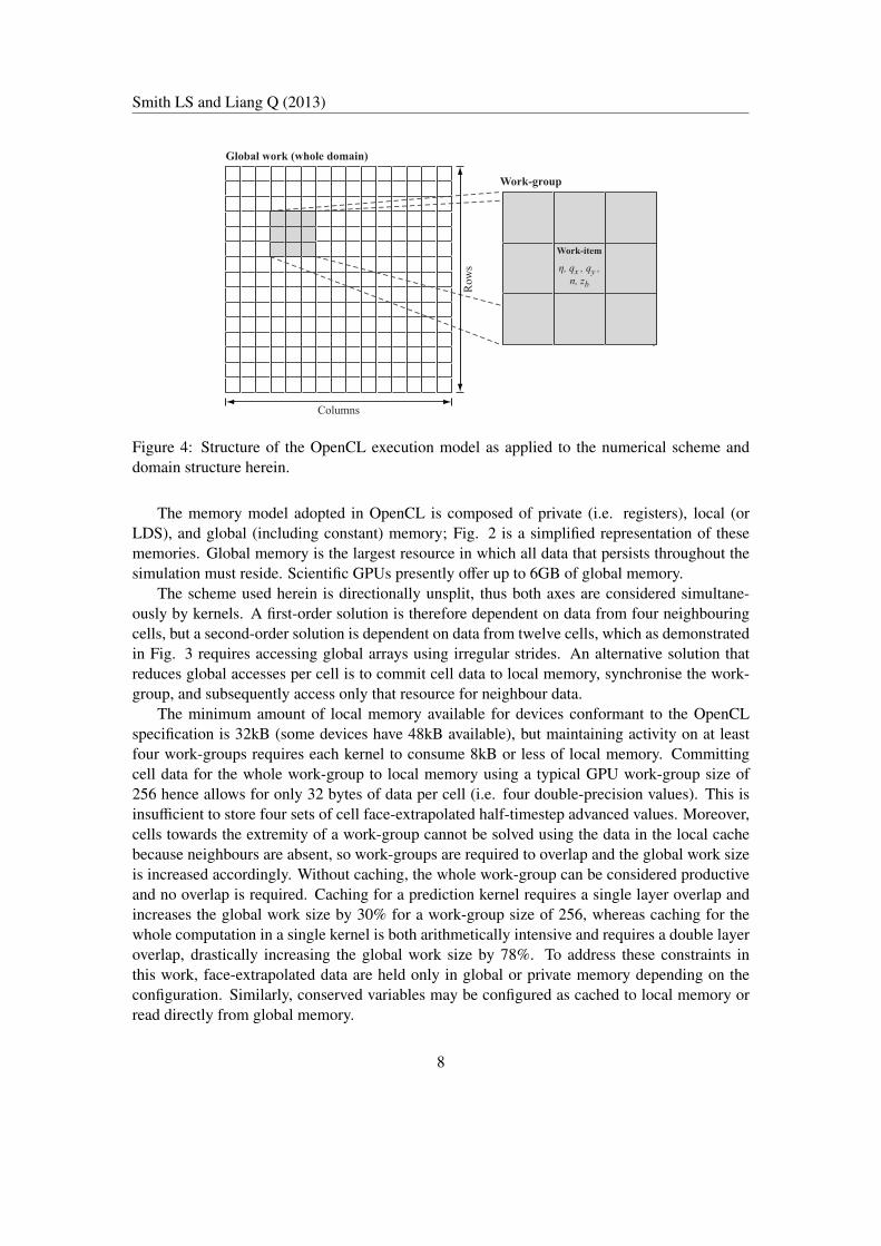
Figure 4: Structure of the OpenCL execution model as applied to the numerical scheme anddomain structure herein.

The memory model adopted in OpenCL is composed of private (i.e. registers), local (orLDS), and global (including constant) memory; Fig. 2 is a simplified representation of thesememories. Global memory is the largest resource in which all data that persists throughout thesimulation must reside. Scientific GPUs presently offer up to 6GB of global memory.

The scheme used herein is directionally unsplit, thus both axes are considered simultane-ously by kernels. A first-order solution is therefore dependent on data from four neighbouringcells, but a second-order solution is dependent on data from twelve cells, which as demonstratedin Fig. 3 requires accessing global arrays using irregular strides. An alternative solution thatreduces global accesses per cell is to commit cell data to local memory, synchronise the work-group, and subsequently access only that resource for neighbour data.

The minimum amount of local memory available for devices conformant to the OpenCLspecification is 32kB (some devices have 48kB available), but maintaining activity on at leastfour work-groups requires each kernel to consume 8kB or less of local memory. Committingcell data for the whole work-group to local memory using a typical GPU work-group size of256 hence allows for only 32 bytes of data per cell (i.e. four double-precision values). This isinsufficient to store four sets of cell face-extrapolated half-timestep advanced values. Moreover,cells towards the extremity of a work-group cannot be solved using the data in the local cachebecause neighbours are absent, so work-groups are required to overlap and the global work sizeis increased accordingly. Without caching, the whole work-group can be considered productiveand no overlap is required. Caching for a prediction kernel requires a single layer overlap andincreases the global work size by 30% for a work-group size of 256, whereas caching for thewhole computation in a single kernel is both arithmetically intensive and requires a double layeroverlap, drastically increasing the global work size by 78%. To address these constraints inthis work, face-extrapolated data are held only in global or private memory depending on theconfiguration. Similarly, conserved variables may be configured as cached to local memory orread directly from global memory.

8


Kernel configuration A Kernel configuration B Kernel configuration C

Load cell & neighbour data to registers

Compute X and Y slope

For each face...

Slope-extrapolate towards faces

Compute flux vector

Evolve cell by half timestep

For each face...


Commit to global memory

Half-timestep kernelLocal mem/cell: 0B

Global accesses: 11 to 14a

Half-timestep kernelLocal mem/cell: 32B


Full-timestep kernelLocal mem/cell: 32B

Global accesses: 2

Load cell data to local memory


For each face...

Slope extrapolate towards faces

Compute flux vector


For each face...


Commit to global memory

Load cell data to local memory

For each neighbour...


For each neighbour’s face...


Compute flux vector


For each neighbour’s face...


For each face...

Non-negative reconstruction

Compute Riemann solution

Compute source terms & flux vector

Update cell state

Load cell & neighbour data to registers

For each face...

Load extrapolations to registers

Non-negative reconstruction

Compute Riemann solution

Compute source terms & flux vector

Update cell state

Full-timestep kernelLocal mem/cell: 0B


Load cell data to registers

Compute and apply discharge change

Update cell state

Implicit friction kernelLocal mem/cell: 0B

Global accesses: 4

a Face extrapolations can be stored in four different arrays for each direction or a structure array containing all faces.

Timestep reduction (identify)

Advance simulation

Figure 5: Implementation of the numerical scheme with three different kernel configurationsintended to suit a majority of modern processing devices, and the data stencils for cell datarequired by each.

Finally, local memory on GPUs is divided into banks (typically 16 or 32); serialisation isrequired for accesses to addresses in the same bank (i.e. conflicts). These can be avoided bymanipulating the dimensions of the cache array to introduce padding, but the increased memoryconsumption may reduce the number of schedulable units running simultaneously.

3.3 Kernel structure

A kernel in OpenCL is executed over the global work (i.e. whole domain), within which thereare work-groups of work-items, as shown in Fig. 4. A different work-item therefore handleseach cell in the domain with reference to data held for neighbouring cells. For a GPU, work-groups are decomposed to schedulable units of wavefronts (AMD) or warps (NVIDIA) for ex-ecution; specifics and vendor differences can be found in Advanced Micro Devices Inc (2011);NVIDIA Corporation (2010a,b); Khronos OpenCL Working Group (2012). Each processing

9


Timestep kernelReduction kernelWork-group 1

Work-group 2

min ∆t

min ∆t

min ∆t

min ∆t

min ∆t

Glo

bal

cel

l st

ate

arra

y

Glo

bal

tim

este

ps

arra

yGlo

bal

work

siz

e

Figure 6: Simplified representation of the two-stage timestep reduction process, with only thefirst two work-groups indicated.

Compute device (OpenCL)

Yes

Yes

No

No

Initialise and load

domain data

Calculate work

dimensions

Compile program

for device

Copy domain data

to device buffers

Queue scheme

kernels

Block until

complete

Write output files to

disk

Release compute

device resources

Simulation

complete?

Output

required?

Queue data read

back to host

Calculate new

queue addition size

Force time

progression

Half-timestep

evolution

Advance simulation

time

Timestep

reduction

Apply friction

effects

Full-timestep

evolution

Host computer (C++)

Figure 7: Flowchart of main operations on the host computer and compute device.

unit should be constantly engaged in productive computation to achieve the best performancewith GPU architectures, known as the level of occupancy. It requires that each processing unitis assigned multiple schedulable units, allowing high-latency operations (e.g. global memoryaccesses, which are equivalent to hundreds of clock cycles NVIDIA Corporation (2010a)) to bemasked by the device’s scheduling. Occupancy generally benefits from a high ratio of arithmeticoperations to global data accesses but scheduling further units delivers no further benefit once ahigh occupancy is already achieved Advanced Micro Devices Inc (2011). Consequently there isno panacea for optimisation on every device when transposing the numerical scheme to kernels.

To achieve high efficiency regardless of vendor differences, user-selectable kernel config-urations are implemented to explore the effects of memory access patterns, illustrated in Fig.5 alongside the data stencils for each kernel. Configuration A is expected to perform well fordevices with a high occupancy and sufficient resources to maintain enough warps/wavefronts tomask global memory latency, thus makes no use of local caching; configuration B introducessome caching to configuration A where possible in the half-timestep kernel, reducing the num-

10


Figure 8: Malpasset dam-break domain, initial conditions and locations of validation points.

ber of global accesses with irregular strides; and configuration C uses the maximum amount ofcaching and the least amount of global accesses, but the consequence is a greater computationalburden because the half-timestep calculation must be repeated many times given that local mem-ory is insufficiently sized to cache face extrapolated data. All high-end devices are expected tohave enough resources (mainly registers) to perform best with configuration A.

3.4 Timestep reduction

A single timestep is used for all cells, identified from the smallest permissible timestep in thedomain. A kernel that iterates through every cell serially is highly inefficient (Amdahl’s Law),hence a two-stage reduction is used here to capitalise on the parallel nature and power of theprocessing units. A fixed global work size is selected and used as the stride through the globalarray of cell data, with each work-item identifying the smallest timestep from those cells it ex-amines. Each work-item commits this data to an array in local memory and binary comparison iscarried out within each work-group, starting at the middle, progressing towards the first element,with work-items successively retired. The first work-item in a work-group commits the lowesttimestep identified in the group to a much smaller global array, which is examined by the singleinstance of the kernel for advancing the overall simulation time. This process is represented inFig. 6. The global work size provides a method of controlling the workload assigned to eachwork-item.

3.5 Kernel scheduling and reduction control

A small overhead is associated with executing kernels and receiving notification of completionwith blocking commands or callbacks. This is alleviated by adding multiple iterations of thenumerical scheme to the execution queue and only displaying progress feedback periodically.Consequently, kernels are occasionally queued unnecessarily, as the simulation cannot progressfurther until output files are written; in such cases the timestep reduces to zero and kernels will

11


Table 1: Total simulation time and cell calculation rate using three different devices, cacheconfigurations and floating-point precisions.

AMD FirePro V7800 NVIDIA Tesla M2075 Intel Xeon E5-2609

Kernel/cache Precision Time (s) Rate (x106/s) Time (s) Rate (x106/s) Time (s) Rate (x106/s)

A: None 32-bit 84 435 66 556 821 45

64-bit 363 106 243 159 1534 25

B: Normal 32-bit 142 258 125 294 956 38

64-bit 446 86 381 101 1730 22

B: Oversized 32-bit 122 300 88 417 951 39

64-bit 442 87 366 105 1739 22

C: Normal 32-bit 122 298 117 314 1136 32

64-bit 844 45 576 67 2818 14

C: Oversized 32-bit 110 335 88 417 1144 32

64-bit 820 47 554 69 2881 13

exit early. The main loops operating on the compute device and host computer to coordinatethis are shown in Fig. 7, where there will be numerous iterations of the OpenCL loop beforereturning to the host computer loop.

4 Results and discussion

Validation of individual elements of the numerical scheme against analytical results for standardtest cases can be found elsewhere in literature Liang (2010); Liang and Marche (2009), hencethis section will focus on evaluating the performance benefits achieved through GPU processing.The results were obtained using an AMD FirePro V7800 GPU with 2GB of memory, an IntelXeon E5-2609 2.40GHz quad-core CPU with access to 24GB of memory, and an NVIDIA TeslaM2075 GPU with 6GB of memory. The value of g is taken to be 9.81ms−2. Comparisons aredrawn between three different hardware devices from each of the mainstream manufacturers forthe same numerical scheme and codebase. Timestep reduction is carried out using 200 work-groups of the maximum size each device will support.

As a uniquely natured event, the Malpasset dam-break is frequently used as a validation test-case for shock-capturing hydraulic models Goutal (1999). The double-curvature arch-dam atMalpasset in the south of France failed catastrophically on the 2nd December 1959 at 9:14PM asit approached full capacity during a period of prolonged and intense rainfall. Almost 55,106m3

of water was released downstream towards Frejus, resulting in over 400 deaths. Data is avail-able from a post-event police survey of the extent and a scale model constructed by EDF. Thepositions of transformers and high-water marks in the valley, plus gauges in the scale model, areindicated in Fig. 8. A regular Cartesian grid of 10m resolution is used to represent the 18km ×

12


Figure 9: Evolving inundation map for the valley every 1000 seconds.

10km domain (1.8M cells). The initial free-surface level behind the dam is 100mAD (estimated0.5m error), and sea level 0mAD. Comparison of results on the left- and right-hand sides of thevalley are presented in Fig. 10 for n = 0.033 (M = 30), the value suggested by CADAM projectparticipants. The first 4000 seconds following the collapse are simulated. Fig. 9 shows theinundation extent in the valley at t = 1000, t = 2000, t = 3000, and t = 4000 seconds.

4.1 CPU-GPU comparison

The run-times with multiple configurations of the software developed herein are presented inTable 1 for the different hardware. The results indicate that for 64-bit computation the NVIDIAGPU model can simulate the Malpasset collapse 6.3x faster than the Intel CPU, while themanufacturer-quoted peak performances suggest a 6.7x difference NVIDIA Corporation (2011);Intel Corporation (2012); the actual and and quoted performance differences for the AMD de-vice are 4.2 and 5.2 respectively Advanced Micro Devices Inc (2012). This is not altogethersurprising; further analysis suggests the AMD device with 64-bit floating-point does not achievefull occupancy because the number of registers constrains the number of wavefronts. Nonethe-less the AMD simulation time represents a significant improvement over the CPU, for a fractionof the cost of an NVIDIA Tesla GPU. Vendor-quoted peak performance levels are rarely achiev-able in practical applications and are compared only to give an indication of device processingpower. For users without a suitable GPU the software will nevertheless provide a significantperformance boost, given that the new software fully harnesses all four cores of the CPU at allstages of the numerical scheme, unlike most existing commercial software.

Caching data to local memory provides no performance benefit with 32- or 64-bit floating-point computation for any of the devices tested herein. Where local memory is used however,oversizing the array is often shown to improve performance by alleviating bank conflicts.

13


10

20

30

40

50

60

70

80

90

P01 P03 P05 P07 P09 P12 P15 P17

Max

imum

wat

er e

leva

tion

(mA

D)

Police survey (right side)Simulation (n=0.033)

10

20

30

40

50

60

70

80

90

P02 P04 P06 P08 P10 P11 P13 P14 P16

Max

imum

wat

er e

leva

tion

(mA

D)

Survey point ID

Police survey (left side)Simulation (n=0.033)

(a) Left-hand side (b) Right-hand side

Figure 10: Comparison of maximum simulated free-surface levels on the left- and right-handsides of the valley (looking downstream) against post-event police survey. Error bars indicateresults for 0.022 ≤ n ≤ 0.100

4.2 Effects of floating-point precision

In all simulations carried out 32-bit computation was faster than 64-bit. There are substantialand significant differences in the results obtained however, which demonstrate that 32-bit in-troduces unacceptably large errors. The spatial distribution of errors in the final and maximumsimulated depths are shown in Fig. 11 and Fig. 12 respectively. Errors in maximum depth areconcentrated in areas with the greatest flow velocities and where shocks are observed immedi-ately downstream of the dam, whereas the final depth errors mainly lie in the shoal zones of thecatchment where water should drain. While the mean error in final depths with SP is < 0.05m,the greatest error was +1.89m, and for the maximum depths the greatest error was +0.85m.The technique adopted herein uses free-surface level as a conserved variable instead of depth,which reduces the numerical resolution of shallow depths in particular. Whilst the localised er-rors may be a by-product of the specific numerical scheme employed herein, we urge cautionand encourage further research before 64-bit precision is dispensed with for performance overaccuracy.

Other authors have previously reported the differences between 32- and 64-bit floating-pointin terms of a mass balance error introduced by successive rounding (e.g. Brodtkorb (2010)),which potentially overlooks the significant magnitude of localised errors. Unlike this study theyconclude that 32-bit floating-point provides an acceptable degree of accuracy. This differencestems from the different numerical scheme employed herein. Mixing different levels of precisionremains a possibility.

14


Figure 11: Spatial distribution of absolute errors introduced in the final depths (4000s) by using32-bit floating-point after the Malpasset collapse, when compared to 64-bit results.

5 Conclusions

In this paper, we have presented how the shallow water equations can be efficiently solved withsecond-order accuracy using a finite-volume Godunov-type scheme and GPUs. Factors affect-ing GPU performance are considered and a range of corresponding configuration parametersdevised to allow the software to be used and optimised with a wide range of modern processors.Simulations of a real-world dam collapse event with the new framework were shown to exhibitgood agreement with a post-event survey, without compromising accuracy but still providingsignificant performance improvements against a CPU. The results demonstrate that the softwaredeveloped herein is appropriate for simulating some of the most challenging flood events, whereshock-like flow discontinuities are present. The new approach will facilitate simulations at res-olutions previously unfeasible across whole cities and large catchments. As further work, wepropose to extend the software to take advantage of multiple GPUs in a single host computer tofacilitate further performance improvements and greater numbers of cells.

32-bit floating-point simulations are shown to introduce significant but localised errors toresults; 64-bit is therefore recommended for flood modelling. Caching cell data to local memoryprovided no direct performance benefit for any of the devices used. Where local memory is used,reducing bank conflicts with array padding is shown to reduce simulation times slightly.

Acknowledgements

This work was generously supported by Advanced Micro Devices, Inc. who provided the ATIFirePro V7800 GPU devices used for the study. The authors also acknowledge the support ofEPSRC through small equipment grants (EP/K031678/1) and doctoral training account.

15


Figure 12: Spatial distribution of absolute errors introduced in the maximum depths by using32-bit floating-point after the Malpasset collapse, when compared to 64-bit results.

ReferencesAdvanced Micro Devices Inc (2011). AMD Accelerated Parallel Processing OpenCL: Programming

guide.Advanced Micro Devices Inc (2012). AMD FirePro Professional Graphics. Accessed: 2013-05-21.Bisson, M., Bernaschi, M., Melchionna, S., Succi, S., and Kaxiras, E. (2012). Multiscale Hemodynamics

Using GPU Clusters. Commun. Comput. Phys., 11:48–64.Brodtkorb, A. R. (2010). Scientific computing on heterogeneous architectures. PhD, University of Oslo.Brodtkorb, A. R., Hagen, T. R., Lie, K., and Natvig, J. R. (2010). Simulation and visualization of the

Saint-Venant system using GPUs. Comput Vis Sci., 13(7):341–353.Brodtkorb, A. R., Saetra, M. L., and Altinakar, M. (2011). Efficient shallow water simulations on GPUs:

Implementation, visualization, verification and validation. Comput & Fluids, 55:1–12.Courant, R., Friedrichs, F., and Lewy, H. (1967). On the partial difference equations of mathematical

physics. IBM J, 11(2):215–234.Crespo, A. C., Dominguez, J. M., Barreiro, A., Gmez-Gesteira, M., and Rogers, B. D. (2011). GPUs,

a new tool of acceleration in CFD: Efficiency and reliability on Smoothed Particle HydrodynamicsMethods. PLoS ONE, 6(6).

Delis, A. I. and Mathioudakis, E. N. (2009). A finite volume method parallelization for the simulation offree surface shallow water flows. Math Comput Simul, 79(11):3339–3359.

Environment Agency (2012). Greater working with natural processes in flood and coastal erosion riskmanagement - a response to Pitt Review recommendation 27. Technical report, Environment Agency.

Erduran, K. S., Kutija, V., and Hewett, C. J. M. (2002). Performance of finite volume solutions to theshallow water equations with shock-capturing schemes. Int J for Numer Methods Fluids, 40(10):1237–1273.

Fang, J., Varbanescu, A. L., and Sips, H. (2011). A comprehensive performance comparison of CUDAand OpenCL. In The 40th International Conference on Parallel Processing (ICPP’11), pages 216–225,Taipei, Taiwan.

French, J. R. (2003). Airborne LiDAR in support of geomorphological and hydraulic modelling. EarthSurf Process Landf, 28:321–335.

Godunov, S. K. (1959). A difference method for numerical calculation of discontinuous solutions of theequations of hydrodynamics (in Russian). Metematicheskii Sbornik, 47(3):271–306.

16


Goutal, N. (1999). The Malpasset dam failure An overview and test case definition. In Proceedings ofthe 4th CADAM meeting, pages 1–8, Zaragoza, Spain.

Haile, A. T. and Rientjes, T. H. M. (2005). Effects of LiDAR DEM resolution in flood modelling: Amodel sensitivity study for the city of Tegucigalpa, Honduras. In ISPRS WG III/3, III/4, V/3 Work-shop ”Laser scanning 2005”, pages 168–173, Enschede, The Netherlands. International Society forPhotogrammetry and Remote Sensing.

Horvath, Z. and Liebmann, M. (2010). Performance of CFD codes on CPU/GPU clusters. In Simos, T. E.,Psihoyios, G., and Tsiotouras, C., editors, ICNAAM Numerical Analysis and Applied Mathematics,International Conference 2010, volume 3, Rhodes, Greece.

Intel Corporation (2012). Intel Xeon Processor E5-2600 Series. Accessed: 2013-05-20.Khronos OpenCL Working Group (2012). The OpenCL Specification v1.2.Kuo, F., Smith, M. R., Hsieh, C., Chou, C., and Wu, J. (2011). GPU acceleration for general conservation

equations and its application to several engineering problems. Comput & Fluids, 45:147–154.Liang, Q. (2010). Flood simulation using a well-balanced shallow flow model. J Hydraul Eng,

136(9):669–675.Liang, Q., Borthwick, A. G. L., and Stelling, G. (2004). Simulation of dam- and dyke-break hydrody-

namics on dynamically adaptive quadtree grids. Int J Numer Methods Fluids, 46(2):127–162.Liang, Q. and Marche, F. (2009). Numerical resolution of well-balanced shallow water equations with

complex source terms. Adv Water Resour, 32(6):873–884.Marks, K. and Bates, P. (2000). Integration of high-resolution topographic data with floodplain flow

models. Hydrol Process, 14:2109–2122.Murillo, J. and Garcıa-Navarro, P. (2010). Weak solutions for partial differential equations with source

terms: Application to the shallow water equations. J Comput Phys, 229(11):4327–4368.Neelz, S. and Pender, G. (2009). Desktop review of 2D hydraulic modelling packages. Technical Report

SC080035, Environment Agency.Nickolls, J. and Dally, W. (2010). The GPU computing era. IEEE Micro, 30(2):56–69.NVIDIA Corporation (2010a). OpenCL Best Practices Guide v3.2.NVIDIA Corporation (2010b). OpenCL programming guide for the CUDA architecture.NVIDIA Corporation (2011). Tesla M-Class GPU Computing Modules. Accessed: 2013-05-20.Owens, J. D., Luebke, D., Godindaraju, N., Harris, M., Kruger, J., Lefohn, A., and Purcell, T. (2007). A

survey of general-purpose computation on graphics hardware. Comp Graph Forum, 26(1):80–113.Pau, J. C. and Sanders, B. F. (2006). Performance of parallel implementations of an explicit finite-volume

shallow-water model. ASCE J Comput Civ Eng, 20(2):99–110.Pender, G. and Neelz, S. (2010). Benchmarking of 2D hydraulic modelling packages. Technical Report

SC080035/SR2, Environment Agency.Roe, P. L. (1986). Characteristic-based schemes for the Euler equations. Annu Rev Fluid Mech, 18:337–

65.Rossinelli, D., Hejazialhosseini, B., Spampinato, D. G., and Koumoutsakos, P. (2011). Multicore/multi-

GPU accelerated simulations of multiphase compressible flows using wavelet adaptive grids. SIAM JSci Comput, 33(2):512–540.

Saetra, M. L. and Brodtkorb, A. R. (2012). Shallow water simulations on multiple GPUs. Lect NotesComput Sci, 7134:55–66.

Schive, H., Zhang, U., and Chiueh, T. (2011). Directionally unsplit hydrodynamic schemes with hybridMPI/OpenMP/GPU parallelization in AMR. Int J High Perform Comput Appl, pages 1–16.

Singh, V. P. and Aravamuthan, V. (1996). Errors of kinematic-wave and diffusion-wave approximationsfor steady-state overland flows. CATENA, 27(3-4):209–227.

Suresh, A. (2000). Positivity-preserving schemes in multidimensions. SIAM J Sci Comput, 22(4):1184–1198.

Toro, E. F. (2001). Shock-capturing methods for free-surface shallow flows. John Wiley and Sons,

17


Hoboken.Toro, E. F., Spruce, M., and Speares, W. (1994). Restoration of the contact surface in the HLL riemann

solver. Shock Waves, 4(1):25–34.van Leer, B. (1984). On the relation between the upwind-differencing schemes of Godunov, Engquist-

Osher and Roe. SIAM J Sci Stat Comput, 5(1):1–20.Wang, P., Abel, T., and Kaehler, R. (2010). Adaptive mesh fluid simulations on GPU. New Astron,

15(7):581–589.Wilkinson, M. E., Quinn, P. F., and Welton, P. (2010). Runoff management during the September 2008

floods in the Belford catchment, Northumberland. J Flood Risk Manag, 3(4):285–295.Xing, Y., Zhang, X., and Shu, C. (2010). Positivity-preserving high order well-balanced discontinuous

galerkin methods for the shallow water equations. Adv Water Resour, 33:1476–1493.Yee, H. C. and Sjogreen, B. (2006). Efficient low dissipative high order schemes for multiscale MHD

flows, II: Minimization of ∇ · B numerical error. J Sci Comput, 29(1):115–164.Zoppou, C. and Roberts, S. (2003). Explicit schemes for dam-break simulations. J Hydraul Eng,

129(11):11–34.

18

towards a generalised gpu cpu shallow-ﬂow modelling tool

Documents