towards a multi-gpu solver for the three-dimensional - · pdf filetowards a multi-gpu solver...
TRANSCRIPT
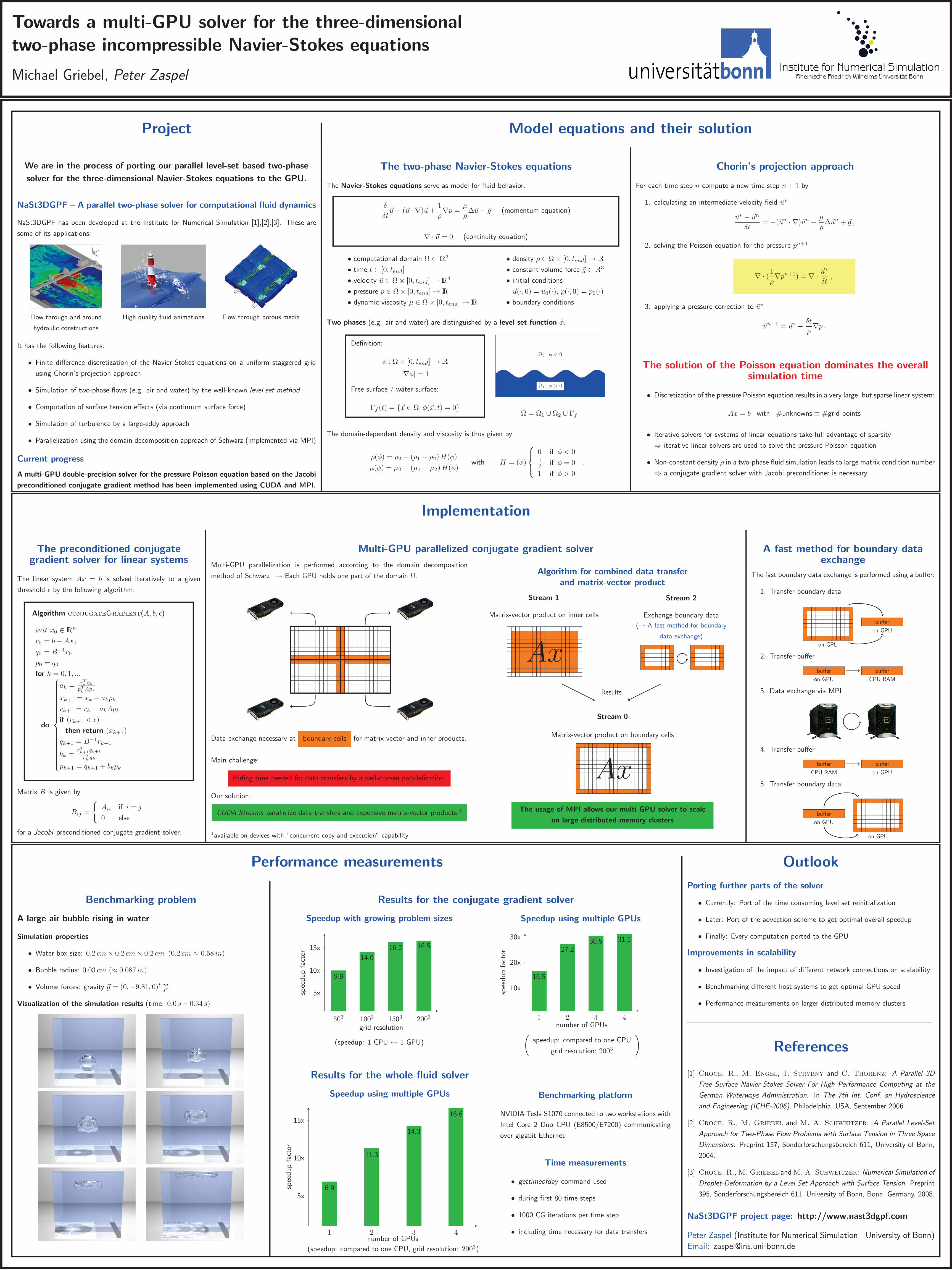
Towards a multi-GPU solver for the three-dimensional
two-phase incompressible Navier-Stokes equations
Michael Griebel, Peter Zaspel
Project Model equations and their solution
We are in the process of porting our parallel level-set based two-phase
solver for the three-dimensional Navier-Stokes equations to the GPU.
NaSt3DGPF – A parallel two-phase solver for computational fluid dynamics
NaSt3DGPF has been developed at the Institute for Numerical Simulation [1],[2],[3]. These are
some of its applications:
Flow through and around
hydraulic constructions
High quality fluid animations Flow through porous media
It has the following features:
• Finite difference discretization of the Navier-Stokes equations on a uniform staggered grid
using Chorin’s projection approach
• Simulation of two-phase flows (e.g. air and water) by the well-known level set method
• Computation of surface tension effects (via continuum surface force)
• Simulation of turbulence by a large-eddy approach
• Parallelization using the domain decomposition approach of Schwarz (implemented via MPI)
Current progress
A multi-GPU double-precision solver for the pressure Poisson equation based on the Jacobi
preconditioned conjugate gradient method has been implemented using CUDA and MPI.
The two-phase Navier-Stokes equations
The Navier-Stokes equations serve as model for fluid behavior.
δ
δt~u + (~u · ∇)~u +
1
ρ∇p =
µ
ρ∆~u + ~g (momentum equation)
∇ · ~u = 0 (continuity equation)
• computational domain Ω ⊂ 3
• time t ∈ [0, tend]
• velocity ~u ∈ Ω × [0, tend] →3
• pressure p ∈ Ω × [0, tend] →
• dynamic viscosity µ ∈ Ω × [0, tend] →
• density ρ ∈ Ω × [0, tend] →
• constant volume force ~g ∈ 3
• initial conditions
~u(·, 0) = ~u0(·), p(·, 0) = p0(·)
• boundary conditions
Two phases (e.g. air and water) are distinguished by a level set function φ.
Definition:
φ : Ω × [0, tend] →
|∇φ| = 1
Free surface / water surface:
Γf (t) = ~x ∈ Ω| φ(~x, t) = 0
Ω1: φ > 0
Ω2: φ < 0
Ω = Ω1 ∪ Ω2 ∪ Γf
The domain-dependent density and viscosity is thus given by
ρ(φ) = ρ2 + (ρ1 − ρ2) H(φ)
µ(φ) = µ2 + (µ1 − µ2) H(φ)with H = (φ)
0 if φ < 01
2if φ = 0
1 if φ > 0
.
Chorin’s projection approach
For each time step n compute a new time step n + 1 by
1. calculating an intermediate velocity field ~u∗
~u∗ − ~un
δt= −(~un · ∇)~un +
µ
ρ∆~un + ~g ,
2. solving the Poisson equation for the pressure pn+1
∇ · (1
ρ∇pn+1) = ∇ ·
~u∗
δt,
3. applying a pressure correction to ~u∗
~un+1 = ~u∗ −δt
ρ∇p .
The solution of the Poisson equation dominates the overallsimulation time
• Discretization of the pressure Poisson equation results in a very large, but sparse linear system:
Ax = b with #unknowns ≡ #grid points
• Iterative solvers for systems of linear equations take full advantage of sparsity
⇒ iterative linear solvers are used to solve the pressure Poisson equation
• Non-constant density ρ in a two-phase fluid simulation leads to large matrix condition number
⇒ a conjugate gradient solver with Jacobi preconditioner is necessary
Implementation
The preconditioned conjugategradient solver for linear systems
The linear system Ax = b is solved iteratively to a given
threshold ǫ by the following algorithm:
Algorithm conjugateGradient(A, b, ǫ)
init x0 ∈ n
r0 = b − Ax0
q0 = B−1r0
p0 = q0
for k = 0, 1, ...
do
ak =rT
kqk
pT
kApk
xk+1 = xk + akpk
rk+1 = rk − akApk
if (rk+1 < ǫ)
then return (xk+1)
qk+1 = B−1rk+1
bk =rT
k+1qk+1
rT
kqk
pk+1 = qk+1 + bkpk
Matrix B is given by
Bij =
Aii if i = j
0 else
for a Jacobi preconditioned conjugate gradient solver.
Multi-GPU parallelized conjugate gradient solver
Multi-GPU parallelization is performed according to the domain decomposition
method of Schwarz. → Each GPU holds one part of the domain Ω.
Data exchange necessary at boundary cells for matrix-vector and inner products.
Main challenge:
Hiding time needed for data transfers by a well-chosen parallelization.
Our solution:
CUDA Streams parallelize data transfers and expensive matrix-vector products.1
1available on devices with “concurrent copy and execution” capability
Algorithm for combined data transferand matrix-vector product
Stream 1
Matrix-vector product on inner cells
Ax
Stream 2
Exchange boundary data
(→ A fast method for boundary
data exchange)
Results
Stream 0
Matrix-vector product on boundary cells
Ax
The usage of MPI allows our multi-GPU solver to scale
on large distributed memory clusters
A fast method for boundary dataexchange
The fast boundary data exchange is performed using a buffer:
1. Transfer boundary data
on GPU
buffer
on GPU
2. Transfer buffer
buffer
on GPU
buffer
CPU RAM
3. Data exchange via MPI
4. Transfer buffer
buffer
CPU RAM
buffer
on GPU
5. Transfer boundary data
on GPU
buffer
on GPU
Performance measurements Outlook
Benchmarking problem
A large air bubble rising in water
Simulation properties
• Water box size: 0.2 cm × 0.2 cm × 0.2 cm (0.2 cm ≈ 0.58 in)
• Bubble radius: 0.03 cm (≈ 0.087 in)
• Volume forces: gravity ~g = (0,−9.81, 0)t ms2
Visualization of the simulation results (time: 0.0 s – 0.34 s)
Results for the conjugate gradient solver
Speedup with growing problem sizes
503 1003 1503 2003
5x
10x
15x
9.9
14.0
16.2 16.5
grid resolution
spee
dup
fact
or
(speedup: 1 CPU ↔ 1 GPU)
Speedup using multiple GPUs
1 2 3 4
10x
20x
30x
16.5
27.230.5 31.1
number of GPUs
spee
dup
fact
or
(
speedup: compared to one CPU
grid resolution: 2003
)
Results for the whole fluid solver
Speedup using multiple GPUs
1 2 3 4
5x
10x
15x
6.9
11.3
14.3
16.6
number of GPUs
spee
dup
fact
or
(speedup: compared to one CPU, grid resolution: 2003)
Benchmarking platform
NVIDIA Tesla S1070 connected to two workstations with
Intel Core 2 Duo CPU (E8500/E7200) communicating
over gigabit Ethernet
Time measurements
• gettimeofday command used
• during first 80 time steps
• 1000 CG iterations per time step
• including time necessary for data transfers
Porting further parts of the solver
• Currently: Port of the time consuming level set reinitialization
• Later: Port of the advection scheme to get optimal overall speedup
• Finally: Every computation ported to the GPU
Improvements in scalability
• Investigation of the impact of different network connections on scalability
• Benchmarking different host systems to get optimal GPU speed
• Performance measurements on larger distributed memory clusters
References
[1] Croce, R., M. Engel, J. Strybny and C. Thorenz: A Parallel 3D
Free Surface Navier-Stokes Solver For High Performance Computing at the
German Waterways Administration. In The 7th Int. Conf. on Hydroscience
and Engineering (ICHE-2006), Philadelphia, USA, September 2006.
[2] Croce, R., M. Griebel and M. A. Schweitzer: A Parallel Level-Set
Approach for Two-Phase Flow Problems with Surface Tension in Three Space
Dimensions. Preprint 157, Sonderforschungsbereich 611, University of Bonn,
2004.
[3] Croce, R., M. Griebel and M. A. Schweitzer: Numerical Simulation of
Droplet-Deformation by a Level Set Approach with Surface Tension. Preprint
395, Sonderforschungsbereich 611, University of Bonn, Bonn, Germany, 2008.
NaSt3DGPF project page: http://www.nast3dgpf.com
Peter Zaspel (Institute for Numerical Simulation - University of Bonn)Email: [email protected]