towards a new methodology for processing scanner data in ... · esbas), which may differ across...
TRANSCRIPT

1
Towards a new methodology for processing
scanner data in the Dutch CPI1
Antonio G. Chessa,2 Stefan Boumans2 and Jan Walschots2
1 The authors want to thank various colleagues, both at Statistics Netherlands and of other statistical offices, for
their continuous support and discussions. The authors also thank Professor Bert Balk for his comments on a previous, different version of the paper. The views expressed in this paper are those of the authors and do not necessarily reflect the policies of Statistics Netherlands. 2 Statistics Netherlands, Team CPI; P.O. Box 24500, 2490 HA The Hague, The Netherlands. Correspondence can be
sent to: [email protected]

2
Abstract This paper presents a new methodology for processing electronic transaction data and for calculating price indices, with the aim of reducing the methodological differences across retailers and consumer goods in the Dutch CPI. Articles (GTINs or EANs) are combined into “homogeneous products”, each of which is defined by a set of article characteristics. Articles that share the same characteristics form a product, which should capture price increases associated with “relaunches” (EAN changes). Two methods for selecting article characteristics are described, which have given the same outcomes. The new index method calculates price indices as a ratio of a turnover index and a weighted quantity index. Weights of homogeneous products are calculated from prices and quantities of multiple periods. Product weights are updated each month in order to incorporate new products timely into the index calculations. Results show that their contribution to a price index may be significant. The method does not lead to chain drift and does not require price imputations. The new methodology is intended to replace the current sample-based methods in the CPI for a department store and for mobile phones in January 2016. Results show clear improvements over the current methods and the previously used survey-based methods. Keywords: Scanner data, CPI, GTIN/EAN, relaunch, product homogeneity, index theory.

3
1. Introduction
Scanner data have clear advantages over traditional survey data collection, notably
because such data sets offer a better coverage of articles sold, sales data offer complete
transaction information (prices and quantities), and the data collection process is
automatised. In spite of their potential, scanner data are still used by a small number of
statistical agencies in their CPI, but the number is likely to increase during the coming
years.3
By scanner data we mean transaction data that specify turnover and numbers of
articles sold by EAN (or GTIN, barcode). At the time of introduction in the Dutch CPI in
2002, scanner data involved two supermarket chains. In January 2010, the data were
extended to six supermarket chains, as part of a re-design of the CPI (de Haan, 2006; van
der Grient and de Haan, 2010; de Haan and van der Grient, 2011). At present, scanner data
of 10 supermarket chains are used and surveys are not carried out anymore for
supermarkets since January 2013. Beside supermarkets, scanner data from other retailers
are used since January 2014. Other forms of electronic data containing both price and
quantity information are obtained from travel agencies, for fuel prices and for mobile
phones. More than 20% of the Dutch CPI is now based on electronic transaction data (in
terms of Coicop weights).
The shift from traditional price collection to electronic transaction data has
introduced new possibilities for developing index methods. Ideally, we would like to
develop a method that makes use of both prices and quantities, and that processes the
transactions of all EANs instead of taking a sample.4 With thousands of EANs per retailer
the question is how to find efficient solutions. This has turned out to be a complex process
over the years, as the current methods in the Dutch CPI differ across retailers and
consumer goods. The current method for supermarket scanner data intends to process all
EANs, but evidences different index related issues. The methods for other retailers make
use of samples of articles.
As the search for new electronic data sources will continue, the question has been put
forward whether a generic index method could be developed that is applicable to different
types of consumer goods and sources (retailers), and that is capable of handling issues
that are not resolved in a fully satisfactory way so far in certain methods (amongst which
the “relaunch” problem and, related to this, the definition of homogeneous products). Such
a method could then also be gradually applied to data sets that are currently in
production, so that the differences in methods used for different retailers can be reduced.
Section 2 gives an overview of the index methods that have been developed for
different electronic transaction data and retailers over the past years in the Dutch CPI. An
outline of a new methodology for processing electronic transaction data is presented in
Section 3. The intention of this section is to show how the new methodology fits within the
CPI system. The aim of the methodology is twofold: (1) to process all EANs, thus
abandoning the traditional approach of selecting a basket of goods, and (2) to have an
index method that deals with the dynamics of an assortment over time, in which new
goods are timely included, and that efficiently handles relaunches.
3 In Europe, six countries will be using scanner data in 2016. The scanner data workshops in Vienna (2014) and
Rome (2015) evidenced that several countries are expecting their first data, while other countries made concrete steps towards acquiring their first scanner data. 4 In this paper, the term “article” and EAN/GTIN are used interchangeably.
4
Sections 4 and 5 elaborate on two essential aspects of the new methodology. The
relaunch problem implies that EANs are not always appropriate as unique identifiers of
homogeneous products. Product homogeneity should then be achieved at a broader level,
at which EANs are combined into groups. Homogeneous products or EAN groups could be
defined by combining EANs that share the same set of characteristics. These have to be
selected in some way. Section 4 proposes and compares two selection methods.
Homogeneous products constitute one of two intermediate article group levels
between the EAN level and the lowest publication level (L-Coicop).5 At the product level,
turnover and quantities of articles sold are summed and used to calculate unit values per
product. These are used to calculate price indices for so-called “consumption segments”,
which combine different homogeneous products (e.g., a segment T-shirts with underlying
products that are described by one or more characteristics).
The index method that has been developed for this purpose is described in Section 5.
A price index for a consumption segment is calculated as the ratio of a turnover index and
a weighted quantity index. The essential element of the index method is the definition and
calculation of the ‘weights’ of the homogeneous products, such that new products can be
directly included. Price indices at Coicop levels are calculated according to conventional
Laspeyres type methods.
Some results obtained with the new methodology are presented in Section 6. Section
7 summarises and concludes with short-term plans with the methodology.
2. Historical overview of methods for processing scanner data
The search for efficient processing methods and index methods for scanner data has
proven to be a challenge throughout the years. Different directions have been investigated
for supermarket scanner data, which may be useful to share with statistical agencies that
are thinking about using scanner data or are about to use scanner data in their CPI. Over
the past 16-17 years, three methods were developed at Statistics Netherlands for
supermarket scanner data, which are referred here to as versions 0, 1 and 2. The choices
and decisions made for these methods are summarised in Table 1.
The first method was proposed at the end of the 1990s. EANs were considered to be a
natural choice for homogeneous products. The availability of weekly turnover data led to
suggesting the Fisher index as an ideal index. Because of frequent assortment changes a
monthly chained Fisher index was considered. However, the price indices showed a strong
downward drift. As a consequence, this method was never implemented.
Based on these experiences, a switch was made to a method that used a (large) basket
and a Laspeyres index with yearly fixed weights. This method was implemented, but
article replacements turned out to be very time consuming as the dynamics of assortments
increased. After seven years it was decided to develop a less labour intensive method.6
The third method (version 2) is the method currently used for supermarket scanner
data. The idea of using a basket of goods was put aside, and a return was made to
processing all transactions. This decision led to adopting a monthly chained index again,
like in version 0. But in the light of the experiences with a strong drifting behaviour, an
5 In the current Coicop classification, L-Coicops are specified at the fifth digit level at most (depending on division).
6 In classical surveys, consumer specialists define ‘representative’ products within Coicops. Overall, the Dutch CPI
contains between 1000 and 1500 of such products. In method version 1, a basket of about 10,000 EANs per retailer was used (Table 1), which makes manual replacement of articles much more difficult.

5
index method was chosen that assigns equal weights to EANs. A drawback of this choice is
that EANs with negligible turnover would receive a relatively high weight. A turnover
threshold was therefore introduced in order to exclude such EANs from the index
calculations (see de Haan and van der Grient (2011) for more details).
Table 1. Methods developed at Statistics Netherlands for supermarket scanner data.
Monthly chained Jevons indices are calculated for consumption segments.7 The price
indices for consumption segments are aggregated to Coicop levels by applying a Laspeyres
index with fixed weights for each consumption segment, which are revised each year. The
impact of equal weights is thus confined to consumption segments.
An important issue with the current method is that relaunches are not handled in a
satisfactory way. Price increases after relaunches are not captured. A so-called “dump
price filter” is introduced in order to prevent price indices from serious downward biases.
Strong price decreases for EANs that are about to be replaced, in combination with low
quantities sold, are filtered out from the calculations. Other practical issues are that the
filter settings need to be tested for each new data set, and possibly also repeated tests
need to be done in the future in order to verify their validity.
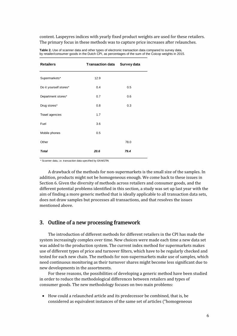
Beside supermarkets, scanner data and other electronic transaction data sets are used
for other retailers. Table 2 shows a complete overview of the retailers and types of
consumer goods. More than 20 per cent of the entire CPI is based on electronic transaction
data (in terms of Coicop weights).
The index methods for retailers other than supermarkets make use of a sample of
EANs. Like in traditional surveys, a limited number of products is defined, for instance, by
picking a small number of brands based on turnover share. EANs are combined into
products based on brand and one or two additional characteristics, such as package
7 In this context, consumption segments are the “internal scanner data aggregates” in Dutch CPI jargon (abbr.:
ISBAs). These ISBAs are our own harmonised reclassification of the retailers’ own classifications of EANs (called ESBAs), which may differ across supermarket chains.
Choices and decisions Version 0 Version 1 Version 2
Developed/used in Late 1990s 2002-2009 2010-present
Sample All data Basket All EANs that satisfy
(± 10,000 EANs certain filters
per retailer)
Homogeneous products EANs EANs EANs
Replacements No Yes, manually No
(EANs with large
turnover share)
Index method Monthly chained Laspeyres, with Monthly chained Jevons,
Fisher index yearly fixed weights with equal weights for
'accepted' EANs;
Laspeyres for (L-)Coicops
Implemented? No Yes Yes
6
content. Laspeyres indices with yearly fixed product weights are used for these retailers.
The primary focus in these methods was to capture price increases after relaunches. Table 2. Use of scanner data and other types of electronic transaction data compared to survey data, by retailer/consumer goods in the Dutch CPI, as percentages of the sum of the Coicop weights in 2015.
A drawback of the methods for non-supermarkets is the small size of the samples. In
addition, products might not be homogeneous enough. We come back to these issues in
Section 6. Given the diversity of methods across retailers and consumer goods, and the
different potential problems identified in this section, a study was set up last year with the
aim of finding a more generic method that is ideally applicable to all transaction data sets,
does not draw samples but processes all transactions, and that resolves the issues
mentioned above.
3. Outline of a new processing framework
The introduction of different methods for different retailers in the CPI has made the
system increasingly complex over time. New choices were made each time a new data set
was added to the production system. The current index method for supermarkets makes
use of different types of price and turnover filters, which have to be regularly checked and
tested for each new chain. The methods for non-supermarkets make use of samples, which
need continuous monitoring as their turnover shares might become less significant due to
new developments in the assortments.
For these reasons, the possibilities of developing a generic method have been studied
in order to reduce the methodological differences between retailers and types of
consumer goods. The new methodology focuses on two main problems:
How could a relaunched article and its predecessor be combined, that is, be
considered as equivalent instances of the same set of articles (“homogeneous
Retailers Transaction data Survey data
Supermarkets* 12.9
Do it yourself stores* 0.4 0.5
Department stores* 0.7 0.6
Drug stores* 0.8 0.3
Travel agencies 1.7
Fuel 3.6
Mobile phones 0.5
Other 78.0
Total 20.6 79.4
* Scanner data, i.e. transaction data specif ied by EAN/GTIN

7
product”)? How could homogeneous products be defined, and how could articles be
matched in an efficient way, without time consuming manual interventions?
What kind of index method could be developed, such that all transactions can be
processed and new articles can be directly included?
The problem of product homogeneity and the index method developed for the above
purposes are treated in sections 4 and 5, respectively. In the present section we sketch
how these components are intended to be integrated into the full CPI production system,
based on our experiences so far with the tests performed with the new methodology.
The processing of electronic data in the Dutch CPI can roughly be subdivided into four
stages:
1. Reading and checking data;
2. Linking articles/EANs to (L-)Coicops;
3. Calculating prices and price indices at “lower aggregate levels”;
4. Calculating price indices for (L-)Coicops and for the CPI as a whole.
The first stage consists of reading data files and performing basic checks on the data, such
as the correctness and completeness of records and record variables and controlling for
quantities sold with value zero (which are isolated before article prices are calculated).
The subsequent three steps are worked out in more detail in the chart of Figure 1. The
“lower aggregate levels” mentioned in step 3 consist of three levels, which are explained
below.
Figure 1. Nested group levels of individual articles in the CPI, and price definitions and price index calculations at these levels in the new methodology.
Article group levels
Consumer goods and services are subdivided in the CPI into Coicops. The most detailed
level of publication within Coicop divisions is referred to as “L-Coicop” in the Dutch CPI.
Scanner data contain transaction data at EAN level. For reasons explained previously, a
(L-)Coicops
Consumption segments
Homogeneous products
Individual articles/EANs
Laspeyres type indices
QU-indices
Product prices (unit values)
Transaction prices
Retailer's ESBAs
Article groups Index calculation

8
further subdivision is made between L-Coicop and EAN level. Individual EANs may have to
be combined into groups, which we refer to as “homogeneous products”. These products
and their underlying articles need to be linked to L-Coicops, which has to be done in an
efficient way if we aim at processing all EANs. For this purpose, it is important to ask
retailers for their own classification of EANs (called ESBAs in our system).
Usually, we take the most detailed ESBA level for establishing the EAN-Coicop links.
However, the most detailed ESBAs may still cover more than one L-Coicop, so that we
need to define an intermediate level between L-Coicops and homogeneous products. This
intermediate level, which we call “consumption segments”, may be derived from more
detailed EAN characteristics (more details are given in Section 4).8
In our first tests with the new methodology, we have chosen consumption segments
to be “types of article”. Examples of segments are men’s T-shirts, ladies’ cardigans or
chocolate. Each of these segments contains a set of homogeneous products. For T-shirts, a
product may contain EANs that have the same number of items per package, the same
sleeve length, fabric and colour. In this way we obtain a nested partition of individual
articles/EANs at different levels, as is shown in Figure 1.
The question is how products can be defined, which article characteristics to select
and what methods could be considered for this purpose. This will be treated in Section 4.
Calculation of price indices
At each level in Figure 1 we either need to define prices or establish the method for
calculating price indices. The price of an individual article is its “transaction price”, that is,
turnover divided by number of articles sold (in fact, this is a unit value at EAN level). For
homogeneous products we use the same definition. Both turnover and quantities sold are
summed over articles that share the same set of selected characteristics. The ratio of these
two sums for groups of articles is usually referred to as a “unit value”.
Unit values and quantities sold for homogeneous products are subsequently used to
calculate a price index for each consumption segment. A new index method is developed
for this purpose, referred to as the “QU-method”, which is described in Section 5. Price
indices for consumption segments are then aggregated to L-Coicops according to
traditional Laspeyres type indices, with weights based on turnover of the preceding year.9
4. Consumption segments and product homogeneity
In order to make choices about consumption segments and homogeneous products,
statistical agencies should ask retailers for information about article characteristics and
article classifications used by retailers for their own purpose (ESBAs). Information about
article characteristics may be contained in article descriptions and also in detailed ESBAs.
Our experiences with electronic data sets are that this information may be supplied in
varying formats by different retailers. For instance, the record variables in drugstore
scanner data are all contained in separate columns (Chessa, 2013). Information about
8 Consumption segments play the same linking role as the ISBA classification in our current system.
9 Aggregation to Coicop levels could also be carried out by applying the aggregation according to the QU-method, by
summing turnover and weighted quantities in the numerator and the denominator of index formula (1) over consumption segments (see Section 5.1). This is a more consistent aggregation method. Preliminary research has shown that the differences between the two aggregation methods are very small at L-Coicop level (Chessa, 2014). As a consequence, we have decided to stick to the traditional way of aggregating to Coicop levels.

9
article characteristics may also be exclusively contained in text strings with EAN
descriptions.
The first example is clearly the preferred data format, as consumption segments and
products can be derived immediately, and EANs can be automatically assigned to both
article group levels and linked to Coicop. In the second case, some form of text mining will
have to be applied in order to retrieve and place information about article characteristics
in separate columns. Text mining falls outside the scope of this paper and will therefore
not be treated further.
Consumption segments are defined as sets of homogeneous products. We have taken
consumption segments to be equivalent with ‘types of article’. Article types can be defined
at different levels of detail (e.g., socks as a whole, or sports, thermal and walking socks as
separate types). In our first tests with department store scanner data, we have defined
article types at the most detailed level of the two mentioned in the example (i.e., sports,
thermal and walking socks). We could say that we differentiate article types, and hence
consumption segments, according to purpose.
Defining tighter consumption segments increases the chance of index imputations.
We come back to this point in Section 6, where a test case is presented. An advantage of
defining tighter consumption segments is that price indices are ‘purer’ in some sense. The
new index method computes weights per unit of product sold (Section 5). In our socks
example, product weights for walking socks are merely based on prices for that article
type and are not mixed with price information and the price index for other types of socks.
In order to avoid potential problems with relaunches, we combine articles into
homogeneous products. This could be done by selecting a set of ‘relevant’ article
characteristics and combine those articles into groups (products) that share the same
characteristics. A walking sock product could contain articles with two pairs of socks per
package, with colour brown and a specific type of fabric. The question is which article
characteristics to select and what methods could be used for this purpose.
Before proceeding, we introduce the following terminology. By “characteristic” of an
article we refer to an instance, a specific value that an article can take. Such a value
belongs to a broader set, which we refer to as “attribute”. For example, ‘white’ is a
characteristic of a T-shirt that belongs to the article attribute ‘colour’.
The selection of article attributes is traditionally part of the consumer specialist’s
domain. Consumer specialists define products by selecting specific characteristics, for
instance, a specific brand name, package content and a consumer target group. We could
build on this idea when using scanner data and supplement it with a sensitivity analysis. A
more technical method could be suggested as an alternative, which belongs to the field of
statistical model selection (Claeskens and Hjort, 2008). We briefly describe both
approaches, which will subsequently be compared with an example.
Sensitivity analysis
The selection of article attributes covers three stages in this approach:
1. For a given consumption segment, the consumer specialist selects a number of article
attributes that (s)he finds to be relevant. This gives rise to an initial set of products;
2. A price index is calculated for the consumption segment, according to the method of
Section 5;
3. A sensitivity analysis is performed: an attribute that was not selected in step 1 is now
added and the price index is re-calculated. If the price index changes ‘significantly’,

10
then the attribute is accepted. This step can be repeated with other attributes.
Attributes may also be omitted when their impact on the price index is negligible.
A meaning has to be given to what is found to be a ‘significant’ impact on a price index
after adding or omitting attributes in step 3. What is found to be an acceptable tolerance?
This may be harder to establish for consumption segments than at Coicop level.
Experience has to be gained with this aspect when the methodology is taken into
production.
Statistical model selection
The point of departure in this approach is a stochastic model for the price of an article.
Following the terminology adopted for the QU-method in Section 5, the price of an article
is decomposed into a product-specific component (the product to which an
article/EAN belongs), a time-specific component (price index with respect to a base
month) and some random (residual) term.
Different sets of attributes may give rise to different numbers of products, and thus
different numbers of product-specific parameters . The problem is to compare different
model versions, with different numbers of free parameters. This can be done by
calculating “information criteria” for each model version, which represent a class of
statistical fit measures that consist of two components:
Under suitable assumptions, the first main term simplifies to a sum of weighted least
squares. The squared differences compare the article transaction prices to the model
prices (or a logarithmic transformation of both prices, depending on the type of
model);
A term that involves the number of free parameters in a model.
The second term acts as a penalty term in assessing model fits. Adding parameters to
a model may decrease the weighted least squares term, but also increases the risk of
overfitting. The aim is to select a model version that balances model fit against model
complexity (number of parameters). The model version with the optimum value of the
information criterion is finally selected.
An advantage of the first method over the second is that it is less technical and, as a
consequence, is expected to be easier to understand among CPI users. An advantage of the
statistical method is that it can be automatised, although this should also be possible with
the first method. The statistical method does not need to specify a ‘tolerance level’, like the
first method. It simply selects that model version, with its corresponding set of
homogeneous products, that optimises the information criterion.
However, there are different types of information criteria, which differ by the size of
the penalty term. This raises the obvious question which one to select. Based on
experiences with scanner data, Chessa (2015) suggests to use the Bayesian Information
Criterion.
A consideration that is not mentioned above is that article attributes may be treated
in different ways. For instance, each package content may be treated as a different value,
thus giving rise to a different product, or different contents give rise to the same product
with quantity-adjustments applied to each.10 It is beyond the scope of this paper to treat 10
This is what we decided in our current method for drugstore scanner data. However, we defined content thresholds in order to keep single item articles separate from multipacks, which are treated as different products.

11
this aspect in detail, but it is important to be aware of the fact that different treatments can
be given to article attributes. It is advisable to compare their impact on a price index.
Example
The new methodology has been tested on scanner data of a department store. Historical
data from the period February 2009 until March 2013 have been used to define
homogeneous products for consumption segments in different Coicops and to test the
index method of Section 5.
We take menswear and ladies’ wear as examples to illustrate the above two methods
for defining products. In the traditional survey for the department store, the consumption
segment T-shirts was characterised by the consumer specialist in terms the following
attributes, for both ladies and men:
Number of items in a package;
Sleeve length;
Colour.
Fabric was not mentioned explicitly, possibly because the consumer specialist had decided
to use an article description with one specific fabric in mind (e.g., standard cotton).
Suppose we exclude fabric initially. Adding fabric as a fourth attribute in a sensitivity
analysis has a very small impact on the price index for men’s T-shirts, but a large impact is
found for ladies’ T-shirts. Fabric should therefore be added to the list of attributes for T-
shirts (which could also be done for both men and ladies in order to limit the number of
different lists of attributes across consumption segments).
Figure 2 shows the price indices for men’s and ladies’ wear for the department store
before and after adding fabric for T-shirts. There is hardly any difference at the L-Coicop
level for menswear, while a small difference can be noted for ladies’ wear (due to the
smaller weight of T-shirts compared to other consumption segments).
The sensitivity analysis gives the same results as the statistical method. For the
consumption segments other than T-shirts, the statistical method even resulted in the
same selection of attributes as was specified by the consumer specialist in the traditional
survey. Based on these results, it may be advisable to start experimenting with the simpler
sensitivity analysis when the new methodology goes into production.
Figure 2. Price indices for menswear and ladies’ wear for a Dutch department store, before and after adding fabric as an extra attribute for T-shirts (Feb. 2009 = 100).
Our primary objective to characterise homogeneous products in terms of a set of
attributes does not necessarily imply that we exclude EANs as product choices in any case.
60
70
80
90
100
110
120
130
140
20
09
02
20
09
05
20
09
08
20
09
11
20
10
02
20
10
05
20
10
08
20
10
11
20
11
02
20
11
05
20
11
08
20
11
11
20
12
02
20
12
05
20
12
08
20
12
11
20
13
02
Menswear
Fabric added for T-shirts Survey-based choices
60
70
80
90
100
110
120
130
140
20
09
02
20
09
05
20
09
08
20
09
11
20
10
02
20
10
05
20
10
08
20
10
11
20
11
02
20
11
05
20
11
08
20
11
11
20
12
02
20
12
05
20
12
08
20
12
11
20
13
02
Ladies' wear
Fabric added for T-shirts Survey-based choices

12
Article characteristics are contained in the EAN descriptions (text strings) for the
department store scanner data. A considerable part of the EAN descriptions only consists
of one to three terms. Defining homogeneous products with such a small number of
attributes may introduce a risk of missing important attributes.
In such cases, one should first contact and visit the retailer and discuss the problem.
Additional information could also be collected through web scraping. But under certain
circumstances it is not needed to collect more information about article characteristics,
which is illustrated by the following examples.
Figure 3 shows the price indices at two levels of product differentiation for the
restaurant part of the department store and for kitchen textiles. Both article assortments
are stable over time, so that calculating price indices with EANs as products does not lead
to problems caused by relaunches. Product differentiation according to a limited set of
attributes (article type, size and taste for the restaurant, and only article type and colour
for kitchen textiles) gives comparable results. No difference was even found for the
restaurant. In cases with short EAN descriptions and stable assortments, the choice of
EANs as homogeneous products can be defended. Moreover, it does not require the
extraction of article characteristics from EAN descriptions, which has been rather time
consuming for the department store data.
Figure 3. Price indices for the restaurant and for kitchen textiles of the department store, for two levels of product differentiation, as calculated with the index method of Section 5 (Feb. 2009 = 100).
5. An index method for consumption segments
5.1 Price index formula
Once consumption segments and the homogeneous products in each segment have
been defined, the question is according to what method price indices could be computed.
The following aspects were considered in our choice of index method:
The index method should be able to incorporate new products in the month of
introduction into the assortment;
Based on our first experience at Statistics Netherlands with scanner data (Version 0,
see Table 1 in Section 2), the method should not suffer from chain drift;
A price index should simplify to a unit value index when all products are
homogeneous.
60
70
80
90
100
110
120
130
140
20
090
2
20
090
5
20
090
8
20
091
1
20
100
2
20
100
5
20
100
8
20
101
1
20
110
2
20
110
5
20
110
8
20
111
1
20
120
2
20
120
5
20
120
8
20
121
1
20
130
2
Restaurant
Products based on attributes EANs as products
60
70
80
90
100
110
120
130
140
20
090
2
20
090
5
20
090
8
20
091
1
20
100
2
20
100
5
20
100
8
20
101
1
20
110
2
20
110
5
20
110
8
20
111
1
20
120
2
20
120
5
20
120
8
20
121
1
20
130
2
Kitchen textiles
Products based on attributes EANs as products

13
Before giving the formulas behind the index method, we introduce some notation. Let
and denote sets of homogeneous products in some consumption segment G in periods 0 and t. The sets of homogeneous products in 0 and t may be different. Let , and
, denote the prices and quantities sold for product , respectively, in period t.11
We denote the price index in period t with respect to, say, a base period 0 by . The
following formula is proposed for calculating price indices (Chessa, 2015):
∑ , ,
∑ , , ⁄
∑ , ∑ , ⁄
. ( )
The numerator is a turnover index, while the denominator is a weighted quantity
(“volume”) index. The product specific parameters are the only unknown factors in
formula (1). Choices concerning the calculation of the are described in Section 5.2.
Price index formula (1) can be written in the following compact form:
⁄
⁄, ( )
where and denote weighted arithmetic averages of the prices and the , respectively,
over the set of products in period t, that is,
∑ , ,
∑ ,
, (3)
∑ ,
∑ ,
. ( )
Notice that the numerator of (2) is equal to the unit value index, where unit values are
defined as the ratio of the sum of turnover and the sum of quantities sold over a set of
products in a consumption segment, as given by (3).
If the products in a consumption segment are homogeneous, then the of all
products have the same value. In this special case, price index (1) simplifies to a unit value
index, a property that we imposed on the index method.12 In the more general case where
a set of products is not homogeneous, then the unit value index must be adjusted. Price
index formula (1) gives a precise expression for the adjustment term, which is the
denominator of (2). This term captures shifts in consumption patterns between different
periods. A shift towards products with higher weights (‘quality’) results in an upward
effect on the volume index and, consequently, in a complementary downward effect on the
price index.
As the method adjusts for shifts between products with different quality, we call index
( ) a “quality adjusted unit value index” (“QU-index” for short). The fundamental question
is how values for the could be obtained. This will be discussed in the next subsection.
11
A different notation is used in this paper from the commonly accepted notation of time as a superscript in prices, quantities and indices. In this paper, preference is given to the notation of both product and time indices as subscripts. This was done in order to reserve the superscript for other purposes (see Chessa (2015), Section 2.3). 12
Time-product dummy and hedonic methods (e.g., see de Haan and Krsinich (2014)) do not satisfy this property.
14
5.2 Choices concerning the
In order to find a method for calculating the product specific weights , we focused
on the following questions:
How could new products be timely incorporated into the index calculations?
The appear in index formula (1) as factors that depend on product, but not on time.
Are the constant in time, or can their values be allowed to vary over time? In the
latter case, how long should we take the periods on which the are constant?
How could chain drift be avoided?
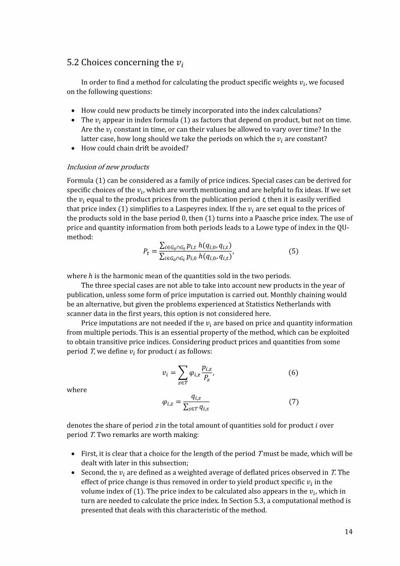
Inclusion of new products
Formula (1) can be considered as a family of price indices. Special cases can be derived for
specific choices of the , which are worth mentioning and are helpful to fix ideas. If we set
the equal to the product prices from the publication period t, then it is easily verified
that price index (1) simplifies to a Laspeyres index. If the are set equal to the prices of
the products sold in the base period 0, then (1) turns into a Paasche price index. The use of
price and quantity information from both periods leads to a Lowe type of index in the QU-
method:
∑ , ( , , , )
∑ , ( , , , )
, ( )
where is the harmonic mean of the quantities sold in the two periods.
The three special cases are not able to take into account new products in the year of
publication, unless some form of price imputation is carried out. Monthly chaining would
be an alternative, but given the problems experienced at Statistics Netherlands with
scanner data in the first years, this option is not considered here.
Price imputations are not needed if the are based on price and quantity information
from multiple periods. This is an essential property of the method, which can be exploited
to obtain transitive price indices. Considering product prices and quantities from some
period T, we define for product as follows:
∑ , ,
, ( )
where
, ,
∑ , ( )
denotes the share of period z in the total amount of quantities sold for product over
period T. Two remarks are worth making:
First, it is clear that a choice for the length of the period T must be made, which will be
dealt with later in this subsection;
Second, the are defined as a weighted average of deflated prices observed in T. The
effect of price change is thus removed in order to yield product specific in the
volume index of (1). The price index to be calculated also appears in the , which in
turn are needed to calculate the price index. In Section 5.3, a computational method is
presented that deals with this characteristic of the method.

15
The index method (“QU-method”) is completely described by formulas ( ), ( ) and
(7). This system of expressions has a counterpart in the field of PPPs, in a method that is
known as the Geary-Khamis (GK) method (Geary (1958), Khamis (1972), Balk (1996,
2001, 2012)). The GK-method has been the subject of some debate, essentially because of
the linear form proposed for the (e.g., see Balk (1996), p. 214). Alternative forms for (6)
are considered in Chessa (2015). These departures from linearity (“perfect substitution”)
were shown to have negligible effects on the price indices analysed, so that it was decided
to stick to the simpler expression (6).
Apart from its simplicity, expression (6) also has another appealing feature. A
straightforward rewriting of (6) gives:
∑ , ,
∑ ,
⁄ . ( )
Expression (8) says that is equal to turnover “in constant prices” of product over
period T, divided by the total number of products sold in the same period. The
numerator in (8) coincides with the notion of volume as used in national accounts. In this
sense, can be defined as volume per unit of product sold.
Returning to our proposal of using prices and quantities from multiple periods for
calculating the , we conclude by comparing some QU-indices with Lowe type index (5),
which is calculated both as a direct index and as a monthly chained index. Figure 4
compares the three price indices for four types of menswear.13 The results show large
differences, which have different causes. While the direct method and the QU-method give
comparable results for socks and underwear, the direct method fails for T-shirts.
Figure 4. QU-indices compared with direct and monthly chained indices (MoM) for four types of menswear, based on scanner data of a department store (Feb. 2009 = 100).
13
In the results shown, T-shirts represent a consumption segment, while the results are aggregated over various consumption segments for the other three article groups.
50
60
70
80
90
100
110
120
130
140
150
20
090
2
20
090
5
20
090
8
20
091
1
20
100
2
20
100
5
20
100
8
20
101
1
20
110
2
20
110
5
20
110
8
20
111
1
20
120
2
20
120
5
20
120
8
20
121
1
20
130
2
Socks
QU-index Direct index MoM index
50
60
70
80
90
100
110
120
130
140
150
20
090
2
20
090
5
20
090
8
20
091
1
20
100
2
20
100
5
20
100
8
20
101
1
20
110
2
20
110
5
20
110
8
20
111
1
20
120
2
20
120
5
20
120
8
20
121
1
20
130
2
Underwear
QU-index Direct index MoM index
5060708090
100110120130140150
20
090
2
20
090
5
20
090
8
20
091
1
20
100
2
20
100
5
20
100
8
20
101
1
20
110
2
20
110
5
20
110
8
20
111
1
20
120
2
20
120
5
20
120
8
20
121
1
20
130
2
T-shirts
QU-index Direct index MoM index
020406080
100120140160180200
20
090
2
20
090
5
20
090
8
20
091
1
20
100
2
20
100
5
20
100
8
20
101
1
20
110
2
20
110
5
20
110
8
20
111
1
20
120
2
20
120
5
20
120
8
20
121
1
20
130
2
Pullovers and Cardigans
QU-index Direct index MoM index

16
The direct method does not capture the contribution of new products to price change
in the year of introduction to the assortment. New types of T-shirts, made of organic
cotton, were introduced in 2010 at high initial prices, which already started to decrease in
2010. The contribution of the new T-shirts is captured by the QU-index, and also by the
monthly chained index, but not by the direct index. The latter only evidences the price
behaviour of the existing part of the assortment, which, in contrast to the new articles,
shows a price increase in 2010.
The monthly chained indices do not come close to the QU-indices in none of the four
cases. This can be partly explained by seasonal effects (e.g., articles returning into the
assortment with price increases, which are missed).
The examples in Figure 4 show that it is important to have an index method in which
not only existing articles enter the calculations, but also new articles. Leaving out new
articles in the year of introduction may have a huge impact on a price index. This implies
that should be calculated for new products as soon as these appear in an assortment.14
Length of the time window T
Scanner data of a large department store and of drugstores, and also electronic data of
mobile phones, have been used to compare time windows that vary between 1 and 4 years
in length. Different window lengths were compared by calculating information criteria
(Section 4).
A unique choice is not easy to make, as different results have been obtained for
different types of goods. One-year windows turned out to give slightly better fits for the
department store scanner data. Longer windows tend to show better fits for drugstore
scanner data, but the differences among the price indices for different window lengths are
negligible in most cases. The same holds for mobile phones. A 1-year window fits well with
current practice in the Dutch CPI and is advantageous with regard to system maintenance
compared to longer windows, as only items sold within one year have to be followed.
The problem of chain drift
We intend to use one-year windows T and the corresponding to calculate price indices
according to expression (1) per publication year. We will do this by using December of the
preceding year as a fixed base month. The choices on the and the length of the time
window T give rise to index numbers that are transitive in publication years, and are
therefore free of chain drift. It is obvious that we need to switch from one set of ’s to
another in the next publication year, a choice that has been motivated by statistical
research on historical data, as mentioned previously.
The method described in Krsinich (2014) offers an alternative to a method with a
fixed base month. She also suggests one-year windows, but proposes to shift the window
along with each publication month (quarter in New-Zealand). Price indices for publication
periods are calculated by chaining year-on-year indices at each shift of the window. The
use of her rolling window approach may lead to large differences compared to our
method.
Different questions and issues have emerged from the comparison with the rolling
window approach. It is not clear how the price indices for different publication years are
related to each other. One would expect the rolling window approach to produce results
14
However, note that new products contribute to a price index from the second month in which they are sold.

17
that are comparable with our method, but with the choice of base month averaged out.
Apparently, this is not the case (Chessa, 2015).
As a final note, it may be interesting to mention that we found a price model with
December as a fixed base month to give structurally better fits than a model based on the
rolling window approach (i.e., the former choice resulted in smaller weighted least
squares values). This finding coincides with current practice in the CPI/HICP, as December
is the month in which yearly weight revisions are carried out.
5.3 Computation of price indices in practice
In order to incorporate new products in a timely way in the index calculations, we
calculate from prices and quantities of the publication year. At this point we encounter a
problem, since we decided upon a model with yearly constant . We refer to the
corresponding index as the theoretical “benchmark index”. The complete set of annual
prices and quantities becomes available only in the final month of a year. This raises the
question how to deal with this problem.
We propose a method for calculating a “real time” version of the benchmark index,
such that:
The are updated each publication month with product prices and quantities which
become available in that month;
Price indices are calculated with respect to the base month, by making use of the
updated . That is, a direct index is used instead of a monthly chained index.
These choices ensure that the benchmark and real time indices are equal at the end of
each year, so that real time indices are free of chain drift as well. This is an important
property of the computational method. The question is how the two price indices compare
in previous months. This will be illustrated in Section 6 with several examples.
Price indices cannot be calculated directly, since the depend on the price indices.
We propose a simple method, which follows an iterative scheme:
1. Suppose that a price index for publication month t has to be calculated. As a first step,
choose initial values for the price indices from base month 0 up to month t;
2. Calculate the for each product sold between the base month and month t by making
use of product prices and quantities up to month t:
∑ , ,
, ( )
where
, ,
∑ ,
. ( )
3. Substitute the obtained in step 2 into expression (1) and calculate updated price
indices up to month t;
4. Repeat steps 2 and 3 until the differences between the price indices obtained in the
last two iterations are ‘small’, according to some pre-defined distance measure.
A number of comments need to be made:

18
The initial values for the price indices in step 1 can be chosen arbitrarily, for instance
, as the algorithm can be shown to converge to a unique
solution (when such a solution exists, of course);
Computation times can be reduced by constructing suitable initial price indices. A
method with this aim is described in Chessa (2015), which has shown that the initial
indices already give very good approximations to the final indices;
The in step 2 are calculated by making use of product prices and quantities from
the base month up to the publication month t. This means that a shorter period is
used at the beginning of each year. As an alternative we could use a moving one-year
window and include data from the preceding year. The results obtained with the
above choices have been satisfactory, as will be shown in Section 6. Therefore we
stick to the method presented above so far, which is simpler to implement;
Price indices are calculated for each month between the base month and the
publication month. However, the price indices up to month t – 1 will not be revised, as
this is not common practice in the CPI (apart from exceptional cases). This means that
only the price index for the publication month will be retained from the calculations,
which hence will not be modified in successive months.
6. First tests with the new methodology
The methodology presented in this paper has been studied and applied to scanner
data of a department store and drugstore chains, and also to transaction data of mobile
phones. It has been implemented for the department store and for mobile phones in a test
environment. The methodology has been programmed in T-SQL for the department store.
It was tested in Excel for mobile phones, as the data set is small (70 devices make up
almost 80% of total turnover). However, the method will be programmed in T-SQL as well
for mobile phones in the near future.
In this section, some first findings are reported with the methodology from tests for
the department store. The following facts show that we are dealing with a big retailer. The
data contain over 133,000 EANs for 2014, which are subdivided into 221 ESBAs according
to the retailer’s article classification. An ESBA gives rise to one or more consumption
segments. The article assortment covers eight Coicop divisions. The department store has
a weight of 0.7 per cent in the Dutch CPI (see also Table 2, Section 2).
One of the key properties of the data is that information about article characteristics
is bundled into text strings. This means that we had to find a way to restructure the data
into a format, such that the price index related problems could be efficiently dealt with. A
method for identifying article characteristics in text strings had to be developed, after
which the characteristics could be placed in separate columns.
A basic form of text mining was used to identify article characteristics. Lists of key
words were set up for the characteristics, based on the coding used by the retailer. The
initial stage of this process consisted of a visual inspection of text strings in order to obtain
a first impression of the coding system. The key word lists were gradually expanded by
isolating the EANs that still did not match the current key words, which could indicate a
different coding for the same characteristic or no coding at all.
This data processing step proved to be time consuming, especially at the beginning. A
retailer may use different ways of coding the same characteristic over time. For instance,

19
we encountered both Dutch and English terms for the same characteristics, and terms
were both spelt out and abbreviated, the latter even in different ways.
Missing information about characteristics can be interpreted in different ways. A
characteristic may not be mentioned when it concerns a ‘default value’. For instance,
single-item packages never have the content of a package mentioned in EAN descriptions,
which, however, is specified for the number of items in multipacks. For data sets like the
scanner data for the department store, one therefore has to try to imagine the logic behind
the retailer’s coding rules. Some degree of interpretation of the EAN descriptions can thus
not be excluded when applying text mining.
The results obtained with text mining were subsequently used to address the
problems related to the calculation of price indices. Historical data over a four-year period
were used for this purpose. Article attributes were selected and homogeneous products
were defined by applying the statistical approach described in Section 4. Choices with
regard to the QU-method were made as well, which are motivated in sections 5.2 and 5.3.
These choices were taken into the implementation and test phase. Price indices have been
calculated according to the scheme in Figure 1 (Section 3), which is worked out in more
detail in Figure 5 below.
Figure 5. Process steps in the implemented methodology for the department store.
The linking of article types and characteristics to EANs, as mentioned in the chart, is
achieved by searching the text strings for corresponding key words.
The chart is in fact generally applicable to any transaction data set. What makes the
chart specifically tailored to the department store data is the possibility to take EANs as
homogeneous products. As was stated in Section 4, this choice was made for consumption
segments with short EAN descriptions and assortments that are stable over time (no or
hardly any relaunch). This choice can be easily made for Coicop divisions 01, 02 and 11, at
least, in case of the department store. For other Coicops, notably for clothing articles,
products are defined in terms of a limited set of attributes (four at most).
A question that comes to mind when looking at the chart in Figure 5 is what to do
with EANs with short descriptions and frequent relaunches. We have not come across
such cases in the department store data. But if such cases would emerge in other data sets,
then some decision must be made. Such cases could be left out when their turnover share
Link article types to EANs in ESBAs
Consumption segment = type of
article
Define consumption segments
Link article characteristics to
EANs
Define homogeneous products Calculate price indices
Product = Combination of characteristics = Group of EANs
Product = EAN
Real time QU-indices for
consumptionsegments
Laspeyres indices for (L-)Coicops
Link article types to retailer's ESBAs
'High' risk of relaunches?
YES NO

20
justifies to do so. Otherwise, some solution has to be found in order to include such EANs.
This is an open problem.
The possibility of choosing EANs as products could be extended to other retailers and
consumer goods, but we prefer to avoid this. The applications of the methodology to
mobile phones and drugstore articles make a consistent choice: products are conceived of
as combinations of article characteristics. The drugstore scanner data show frequent
relaunches, which take place in most of its assortment.
Price indices for consumption segments are calculated according to the algorithm in
Section 5.3, which computes real time indices. The resulting indices are free of chain drift,
as they are equal to the theoretical benchmark indices, with yearly fixed product specific
parameters , at the end of each year. But these parameters are updated each month
when calculating real time indices for each publication month, so the question was raised
to what extent the real time and benchmark indices differ.
Both indices were compared during the validation of the first test results. Some
results are shown in figures 6-8, for consumption segments in three Coicop divisions. The
real time indices are the indices that would be published in the CPI. The results show
hardly any difference between the real time and benchmark indices. This has been
observed so far throughout almost the entire assortment. An exceptional case is ladies’ T-
shirts in Figure 7. Differences may typically occur in the first months of a year, as price and
quantity data from shorter time windows are used to calculate the .
Figure 6. Real time and benchmark indices for cake and crisps, based on scanner data for the department store from recent years (Dec. 2012 = 100).
Figure 7. Real time and benchmark indices for men’s and ladies’ T-shirts (Dec. 2012 = 100).
As was suggested in Section 5.3, a moving one-year window could be used, adding
price and quantity data from the preceding year. This is a point worth investigating in
subsequent tests of the index method. The real time and benchmark indices for all other
ladies’ clothing articles show negligible differences or no difference at all. At aggregate
0
20
40
60
80
100
120
140
160
180
200
20
121
2
20
130
2
20
130
4
20
130
6
20
130
8
20
131
0
20
131
2
20
140
2
20
140
4
20
140
6
20
140
8
20
141
0
20
141
2
20
150
2
Cake
Benchmark Real time index
0
20
40
60
80
100
120
140
160
180
200
20
121
2
20
130
2
20
130
4
20
130
6
20
130
8
20
131
0
20
131
2
20
140
2
20
140
4
20
140
6
20
140
8
20
141
0
20
141
2
20
150
2
Crisps
Benchmark Real time index
0
20
40
60
80
100
120
140
160
180
200
20
121
2
20
130
2
20
130
4
20
130
6
20
130
8
20
131
0
20
131
2
20
140
2
20
140
4
20
140
6
20
140
8
20
141
0
20
141
2
20
150
2
Men's T-shirts
Benchmark Real time
0
20
40
60
80
100
120
140
160
180
200
20
121
2
20
130
2
20
130
4
20
130
6
20
130
8
20
131
0
20
131
2
20
140
2
20
140
4
20
140
6
20
140
8
20
141
0
20
141
2
20
150
2
Ladies' T-shirts
Benchmark Real time
21
levels, the impact of the difference for ladies’ T-shirts will therefore be small, if not
negligible.
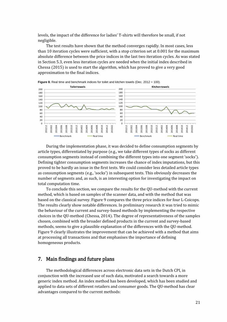
The test results have shown that the method converges rapidly. In most cases, less
than 10 iteration cycles were sufficient, with a stop criterion set at 0.001 for the maximum
absolute difference between the price indices in the last two iteration cycles. As was stated
in Section 5.3, even less iteration cycles are needed when the initial index described in
Chessa (2015) is used to start the algorithm, which has proved to give a very good
approximation to the final indices.
Figure 8. Real time and benchmark indices for toilet and kitchen towels (Dec. 2012 = 100).
During the implementation phase, it was decided to define consumption segments by
article types, differentiated by purpose (e.g., we take different types of socks as different
consumption segments instead of combining the different types into one segment ‘socks’).
Defining tighter consumption segments increases the chance of index imputations, but this
proved to be hardly an issue in the first tests. We could consider less detailed article types
as consumption segments (e.g., ‘socks’) in subsequent tests. This obviously decreases the
number of segments and, as such, is an interesting option for investigating the impact on
total computation time.
To conclude this section, we compare the results for the QU-method with the current
method, which is based on samples of the scanner data, and with the method that was
based on the classical survey. Figure 9 compares the three price indices for four L-Coicops.
The results clearly show notable differences. In preliminary research it was tried to mimic
the behaviour of the current and survey-based methods by implementing the respective
choices in the QU-method (Chessa, 2014). The degree of representativeness of the samples
chosen, combined with the broader defined products in the current and survey-based
methods, seems to give a plausible explanation of the differences with the QU-method.
Figure 9 clearly illustrates the improvement that can be achieved with a method that aims
at processing all transactions and that emphasises the importance of defining
homogeneous products.
7. Main findings and future plans
The methodological differences across electronic data sets in the Dutch CPI, in
conjunction with the increased use of such data, motivated a search towards a more
generic index method. An index method has been developed, which has been studied and
applied to data sets of different retailers and consumer goods. The QU-method has clear
advantages compared to the current methods:
0
20
40
60
80
100
120
140
160
180
200
20
121
2
20
130
2
20
130
4
20
130
6
20
130
8
20
131
0
20
131
2
20
140
2
20
140
4
20
140
6
20
140
8
20
141
0
20
141
2
20
150
2
Toilet towels
Benchmark Real time
0
20
40
60
80
100
120
140
160
180
200
20
121
2
20
130
2
20
130
4
20
130
6
20
130
8
20
131
0
20
131
2
20
140
2
20
140
4
20
140
6
20
140
8
20
141
0
20
141
2
20
150
2
Kitchen towels
Benchmark Real time

22
Figure 9. Price indices for the QU-method, the current method and the previously used survey-based method for four L-Coicops (Feb. 2009 = 100).
The classical approach of following prices for a basket of goods can be abandoned and
replaced by integral processing of transaction data;
This can be achieved without introducing and testing data filters. Of course, it is wise
to apply certain filters (e.g., for outlier detection);
New products can be incorporated into the index calculations in a timely way. The
availability of an index method that is capable of doing this has clearly proven its
usefulness and superiority over methods that postpone the inclusion of new products
until the next year (see Figure 4, Section 5.2);
There is no need to impute prices of products within consumption segments. A
product that is not sold in some period simply does not contribute to turnover and
volume (weighted quantity) in that period. If the same product is sold in a different
period, then it contributes to turnover and volume for that period. So, the weighted
quantity measure handles products that are not sold in certain periods without any
problem and need for imputation.
The aim of timely including new products in an index method adds notable
complexity to the quest for such a method. Product weights need to be based on price and
sales information from the current publication year. The computational method described
in Section 5.3 makes use of monthly updated weights, which consequently will vary over
time. One of the key features of the method is that it is benchmarked to a method with
yearly fixed weights, which is transitive, and therefore enables us to obtain price indices
that are free of chain drift within a publication year. The product weights are allowed to
vary over years, a choice that was motivated by statistical analyses, in which time
windows of different length were compared.
The methodology has been extensively applied to different electronic transaction data
sets. It has been implemented and tested for scanner data of a department store and for
60
70
80
90
100
110
120
130
1402
00
90
2
20
09
05
20
09
08
20
09
11
20
10
02
20
10
05
20
10
08
20
10
11
20
11
02
20
11
05
20
11
08
20
11
11
20
12
02
20
12
05
20
12
08
20
12
11
20
13
02
Menswear
QU-index Current method Survey
60
70
80
90
100
110
120
130
140
20
09
02
20
09
05
20
09
08
20
09
11
20
10
02
20
10
05
20
10
08
20
10
11
20
11
02
20
11
05
20
11
08
20
11
11
20
12
02
20
12
05
20
12
08
20
12
11
20
13
02
Ladies' wear
QU-index Current method Survey
60
70
80
90
100
110
120
130
140
20
09
02
20
09
05
20
09
08
20
09
11
20
10
02
20
10
05
20
10
08
20
10
11
20
11
02
20
11
05
20
11
08
20
11
11
20
12
02
20
12
05
20
12
08
20
12
11
20
13
02
Bed linen
QU-index Current method Survey
60
70
80
90
100
110
120
130
140
20
09
02
20
09
05
20
09
08
20
09
11
20
10
02
20
10
05
20
10
08
20
10
11
20
11
02
20
11
05
20
11
08
20
11
11
20
12
02
20
12
05
20
12
08
20
12
11
20
13
02
Table linen and bathroom linen
QU-index Current method Survey

23
transaction data of mobile phones. Some of the findings that have emerged from the
analysis of the test results can be summarised as follows:
Most of the differences between the benchmark and real time indices are negligible or
show no difference at all;
Larger differences have been noted in some exceptional cases for the department
store data, which typically arise in the first months of a year due to the use of a
shorter time window for calculating the product weights;
These differences could be reduced by extending the time window with months of the
preceding year. Although this is an interesting option for further research, it does not
seem to be a big issue so far;
The results have been validated and are in agreement with theoretical expectations
about the behaviour of the price indices.
The department store data required quite some time in extracting article
characteristics from the EAN descriptions. This investment of time eventually paid off, as
the linking of article characteristics to EANs operates through a short list of key words that
has remained stable over time (for almost 7 years of data now).
Based on this finding, we expect monthly maintenance work to be limited. Most of this
work will be on controlling new EANs on whether they contain new types of articles and
attributes. With the aid of the current list of search items, new types of articles should be
rather easy to isolate. New consumption segments should therefore be easy to identify.
If the new article types possess attributes that have not been identified so far, then
the current list of key words should be extended with new characteristics. Attributes
should then be selected in order to define homogeneous products for the new segments,
which can be handled by applying one of the two approaches described in Section 4 (we
will start experimenting with the simpler one). This would require most of the
maintenance work. The exact implications in terms of time will become clear next year,
after taking the methodology into production.
Statistics Netherlands intends to take the methodology into production in January
2016, both for the department store and for mobile phones. The methodology then will
replace the current sample-based methods. The methodology has also been studied and
applied to scanner data for drugstores and do-it-yourself stores. Additional data are
needed for both data sets, as questions on discounts and product homogeneity have been
raised. In order to resolve these issues, the first step should be to contact retailers. We
have received a test data set for the do-it-yourself stores with additional information. In
addition, the test data is better structured than the original data, which should even
reduce text mining.
Statistics Netherlands has defined a research program for the coming years, which
aims at studying possibilities for further improvement of the methodology, ranging from
text mining and data analysis/exploration to price index methods. This research will be
extended to other scanner data sets, amongst which supermarkets.
To conclude, Statistics Netherlands is putting a lot of effort into collecting internet
prices through web scraping. However, considerable care is needed when using such data
to compile price indices, as numbers of articles sold are not available. Methods that assign
equal weights to articles generally give poor statistical fits to price data and the resulting
price indices may differ considerably from price indices in which articles are weighted
according to turnover shares (Chessa, 2014, 2016). Information from additional sources is

24
therefore needed in order to use internet prices in a meaningful way. If it is possible to
obtain turnover share type of weights, then this would open possibilities to apply the QU-
method to internet data as well.
References
Balk, B.M. 1996. A comparison of ten methods for multilateral international price and
volume comparison. Journal of Official Statistics, 12: 199-222.
Balk, B.M. 2001. Aggregation methods in international comparisons: What have we
learned? Paper originally prepared for the Joint World Bank - OECD Seminar on
Purchasing Power Parities, 30 January - 2 February 2001, Washington DC.
Balk, B.M. 2012. Price and Quantity Index Numbers: Models for Measuring Aggregate Change and Difference. Cambridge, UK: Cambridge University Press.
Chessa, A.G. 2013. Comparing scanner data and survey data for measuring price change of
drugstore articles. Paper presented at the Workshop on Scanner Data for HICP, 26-27
September 2013, Lisbon.
Chessa, A.G. 2014. An index method for a Dutch department store. The Hague: Statistics
Netherlands. (In Dutch)
Chessa, A.G. 2015. Towards a generic price index method for scanner data in the Dutch
CPI. Ottawa Group Meeting, 20-22 May 2015, Urayasu City, Japan.
Chessa, A.G. 2016. Product homogeneity and weighting when using scanner data for price
index calculation. Invited paper at the 2016 International Methodology Symposium “Growth in Statistical Information: Challenges and Benefits”, 22-24 March 2016, Gatineau,
Quebec, Canada. (In preparation)
Claeskens, G. and N.L. Hjort. 2008. Model Selection and Model Averaging. Cambridge, UK:
Cambridge University Press.
Geary, R. C. 1958. A note on the comparison of exchange rates and purchasing power
between countries. Journal of the Royal Statistical Society A, 121: 97-99.
van der Grient, H.A. and J. de Haan. 2010. The use of supermarket scanner data in the
Dutch CPI. Paper presented at the Joint ECE/ILO Workshop on Scanner Data, 10 May 2010,
Geneva.
de Haan, J. 2006. The re-design of the Dutch CPI. Statistical Journal of the United Nations Economic Commission for Europe, 23: 101-118.
de Haan, J. and H.A. van der Grient. 2011. Eliminating chain drift in price indexes based on
scanner data. Journal of Econometrics, 161: 36-46.

25
Haan, J. de, and F. Krsinich. 2014. Time dummy hedonic and quality-adjusted unit value
indexes: Do they really differ? Paper presented at the 1st Conference of the Society for
Economic Measurement, 18-20 August 2014, University of Chicago.
Khamis, S. H. 1972. A new system of index numbers for national and international
purposes. Journal of the Royal Statistical Society A, 135: 96-121.
Krsinich, F. 2014. The FEWS Index: Fixed Effects with a Window Splice – Non-revisable
quality-adjusted price indexes with no characteristic information. Paper presented at the
Meeting of the group of experts on consumer price indices, 26-28 May 2014, Geneva,
Switzerland.