Towards a Theory of Trade Finance∗

Tim Schmidt-Eisenlohr

European University Institute

December 7, 2009

Abstract

Cross border transactions are conducted using different payment contracts, the usageof which varies across countries and over time. In this paper I build a model thatcan explain this observation and study implications from this for international trade.In the model exporters optimally choose payment contracts, trading off differencesin enforcement and efficiency between financial markets in different countries. Ifind that the ability of firms to switch contracts is central to the reaction of tradeto variations in financial conditions. Numerical experiments with a two-countryversion of the model suggest that limiting the choice between payment contractsreduces traded quantities by up to 60 percent.

JEL: F12, F3, G21, G32Keywords: trade finance, payment contracts, trade patterns, financial crisis

∗ I am grateful to Giancarlo Corsetti, Russell Cooper and Omar Licandro for constant advice. I would alsolike to thank Andrew Bernard, Jonathan Eaton and participants of the the Cooper & Students Discussion Groupand the Macro Student Lunch at the European University Institute for useful comments.

1 Introduction

Transactions in international trade are conducted using different payment contracts. These can

be broadly classified into Cash in Advance, Open Account and bank intermediated contracts.

Evidence suggests that usage of payment contracts varies both across countries and over time.

Current trade theory does not address these contracts. To understand why different payment

contracts are used by different firms and what effects these have on international trade, a suitable

model is needed.

In this paper I develop a theory of trade finance that explains the co-existence of the different

financing forms depending on enforcement and cost of financing, and analyze the trade-offs faced

by exporters. The model shows that the impact of variations in financial conditions on trade

significantly depends on the ability of firms to switch contracts. Furthermore, it predicts that the

choice of payment contract shapes variable trade costs and that FOB prices vary systematically

with payment contracts and financial market conditions. In a two-country version of the model

numerical experiments are conducted. I find that limiting the choice between payment contracts

reduces traded quantities by up to 60 percent. In an extension I introduce repeated transactions

and show that these can explain the empirical observation that trade credit intensive industries

are less affected by a financial crisis.

While several recent papers have analyzed the effect of the exporter’s financial market on

participation decisions or exported quantities, none have examined the interaction of financial

conditions in the sending and receiving countries. A setup featuring the choice of payment

contract between an importer and an exporter has not been studied before. Taking into account

characteristics of both financial markets gives rise to interesting interactions. Depending on

which payment contract is chosen by an exporter, different parameters of the two financial

markets are relevant. Choosing a payment contract allows to substitute away from the least

favorable conditions. In a model taking into account the exporter financial market only, this

substitution is not possible. Then, exporters are fully affected by any changes of financial

conditions in their market.

I model three types of payment contracts: Cash in Advance (CIA), Open Account (OA)

and Letter of Credit (LC). With Cash in Advance, the importer pays the trade before receiving

the goods. Under Open Account the importer only pays after receiving the goods. The third

payment contract considered is a Letter of credit, in which banks act as intermediaries resolving

1

the enforcement problem.1

The main findings are as follows. CIA is more likely to be used if enforcement at home

is strong and if financing costs abroad are low. OA is more likely if enforcement abroad is

strong and financing costs at home are low. LC is used if enforcement is relatively weak and

interest rate costs are relatively low in both countries. Costs arising from trade finance take

the form of variable costs that are proportional to the value traded, i.e. they correspond to

the iceberg formulation often used in international trade. When financing costs or enforcement

probabilities change, firms can react by switching payment contracts. In this respect, the time

horizon in which firms are able to switch payment contracts is important. In the very short

run switching contract might be difficult. It could imply a fixed cost, which would limit the

switching. However, in the short run it could still be easier to switch to a different payment

contract between two trading partners than to switch bank for any of them.

When repeated transactions are considered, under certain conditions, trigger strategies can

improve on the one shot equilibria when CIA or OA are used. These trigger strategies are

more likely to be optimal when the expected number of repeated transactions is large and when

enforcement probabilities are high. In this case CIA and OA become more attractive relative to

a LC. This prediction is in line with the notion that LCs are used relatively more when trade

relationships have a shorter time horizon, whereas especially OA is more common in long term

relationships. It can also explain the finding that trade relationships, in which more trade credit,

i.e CIA and OA, is used, might be less affected by financial crisis than relationships using trade

credit less intensively, as reported by Levchenko, Lewis, and Tesar (2009).

The model predicts asymmetric reactions of trade flows to financial turmoil. If there is

country-specific financial turmoil, firms are able to partially mitigate adverse effects by switching

payment contracts. If there is global financial turmoil that affects both the financial markets

of the exporter and the importer, this possibility does no longer exist and trade flows react

more strongly to a crisis. This suggests that in the current global financial crisis trade finance

might have a stronger effect on aggregate trade flows than in former more locally concentrated

ones. The model predicts differences between South-North and South-South trade volumes that

are absent in models on financing constraints in which only the exporter’s financial market

conditions play a role. There is an additional effect of the choice of payment contract on FOB1I represent all bank intermediated transactions by the LC. They usually involve banks both in the importer’s

and exporter’s country and the usage of some form of documentation upon which payment is being made bya bank to the exporter. For an introduction to the different types of trade finance payment contracts see U.S.Department of Commerce (2008).

2

prices besides determining a part of variable trade costs. As the payment contract arranges

who has to bear financing costs, the payment to be paid by the importer can be discounted

depending on the timing of the transaction.

There are several theoretical papers that have addressed the issue of financial market con-

ditions and international trade. Kletzer and Bardhan (1987) show how sovereign default risk

and credit market imperfections can result in differences in interest rates and tightness of credit

rationing in equilibrium respectively and thus create comparative advantage. In Matsuyama

(2005) the share of revenues an entrepreneur can pledge towards wage payments differs between

countries leading to comparative advantage.2

Chaney (2005) develops a theoretical model analyzing financial constraints in a heterogenous

firms trade model based on Melitz (2003). Firms have to finance their fixed entry cost into

foreign markets through own liquidity and domestic operating profits. Liquidity is introduced

as a second type of heterogeneity. He derives conditions on productivity and liquidity under

which a firm exports. Manova (2008) extends this model and estimates it using the methodology

suggested by Helpman, Melitz, and Rubinstein (2008). She introduces a default probability

similar to the one used in this paper. While in her model there is a domestic enforcement

problem between a bank and a firm, in this paper the enforcement problems arise between firms

in different countries.

Her model has been further extended to a dynamic setting taking into account capital accu-

mulation by Suwantaradon (2008). In Chaney (2005), Manova (2008) and Suwantaradon (2008)

only domestic financial market conditions are relevant for the exporting decisions of firms. In

this paper in contrast the effects of conditions in the financial markets of both the exporter and

the importer, determined by the optimal choice between payment contracts, are analyzed.

Some articles study empirically the interaction between financial conditions and trade. The

role of financial development for trade in manufactures is studied in Beck (2002) and Beck

(2003). Using data from 65 and 56 countries respectively he finds that financial development of

a country has a strong effect on export volumes of manufactures and that this effect is stronger

in external finance intensive industries.3

Some recent papers test for effects of financial constraints on the extensive margin of trade

using firm level data. Greenaway, Guariglia, and Kneller (2007) use UK manufacturing firm level2The broader issue of institutional constraints, trade and outsourcing has been studied extensively. For a

survey see Helpman (2006).3Svaleryd and Vlachos (2005) find evidence on patterns of industrial specialization and financial market con-

dition that point in the same direction.

3

data and find no evidence for a causal effect of ex-ante financial health on export participation.

French firm level data analyzed by Berman and Hericourt (2008) seems to point in the opposite

direction.4

There is a policy debate on the effects an importance of trade finance in general and during a

financial crisis.5 The effects of financial crisis on trade have been assessed empirically by several

papers. Ronci (2004) analyzes data from 10 financial crises and finds evidence for a negative

effect of financial crises both on imports and exports. Iacovone and Zavacka (2009) analyze

data from 23 banking crises. They find a differential effect of a banking crisis on firms that

rely on bank finance versus firms that rely on inter-bank credit. This supports the prediction of

the model that inter-firm credit relations are an important factor for mitigating financial crisis.

Evidence on firm level trade finance of African exporters is documented by Humphrey (2009).

Berman and Martin (2009) analyze how financial crisis affects trade and find that disruption

from financial crisis is stronger and longer lasting for African than for other countries. Using data

on U.S. imports, Levchenko, Lewis, and Tesar (2009) analyze causes of the current international

trade decline and argue that trade credit did not play a role. I discuss in Section 5 on repeated

contracts how this finding can be explained and why trade finance might be more important

than suggested by this result. Amiti and Weinstein (2009) use data on Japanese exporters

matched with Japanese banks to study the transmission of financial shocks during the financial

crisis in the 1990s. They find that one third of the decline in Japanese exports in that period

can be explained by a bank firm trade finance channel. This confirms the relevance of financing

conditions on the side of the exporter. The theory proposed here suggests, that in addition to

this, there are effects arising from the financing conditions of the importer and the interaction

of the two.

The rest of the paper is organized as follows. Section 2 develops a microeconomic model of the

choice of payment contract. Section 3 puts this model into an intra-industry trade framework.

Section 4 derives the general equilibrium and studies a quantitative example. Section 5 extends

the analysis to repeated transactions. Section 6 discusses implications of payment contracts

during financial crisis, on trade patterns, and on FOB prices. Section 7 concludes.4Other papers analyzing this are Berthou (2007), Espanol (2007), Berthou (2008), Stiebale (2008) and Bellone,

Musso, Nesta, and Schiavo (2008). Zia (2008) analyzes the effects of export subsidies on exporting behavior.Baltensperger and Herger (2007) test the effects of export insuring schemes.

5See Stephens (1998), Auboin and Meier-Ewert (2003) and Auboin (2007). In the context of the currentfinancial crisis trade finance has received a renewed attention. See Chauffour and Farole (2009) and Dorsey(2009).

4

2 Payment Forms

2.1 Overview

There are three types of payment contracts available to finance trade transactions: Cash-in

Advance, Open Account and Bank Intermediated transactions.

Figure 1 based on data from IMF (2009) illustrates some survey evidence on the usage of

these different payment forms.6 While Open Account seems to be the dominant financing form,

the share of the other two groups is also quantitatively important. The survey suggests that

during the current financial crisis the usage of open account has declined, whereas the two pay-

ment forms that limit the risk of exporters have increased their shares. This evidence is in line

with the prediction of the model that changes in financial market conditions cause switches of

payment contracts. Evidence on the effect of the crisis on the choice of payment forms in ICC

(2009) suggests that the current crisis might lead to a renaissance of the Letter of Credit. That

is, given rising uncertainty, firms rely more on the safest payment contract available, which

is the Letter of Credit. It is also stated there that 50-60 percent of China’s foreign trade is

financed with LCs. This indicates that in a less financially developed country like China bank

intermediated transactions are used relatively more often.

Here figure 1

2.2 Micro Model

The following section introduces a simple microeconomic model for the choice of finance of an

exporter. Besides transport costs, I consider two additional cost factors in international trade

relative to domestic trade. First, the time delay between production and the realization of sales

is longer for international than domestic transactions. Hummels (2001) discusses the effect of

physical transport time while Djankov, Freund, and Pham (2006) analyze the effect of time delay

from the factory gate to the means of transportation on international trade. Both show that

international trade has a relevant time dimension. The latter document that procedures specific

to trade across international borders are responsible for additional delays. Second, enforcement

at the international level is more difficult than domestically.7 This can be due to differences in6Unfortunately to my knowledge currently only survey data is available. Thus the numbers should be seen as

a reference point.7Enforcement might also be a problem at the domestic level. In the model I abstract from this and analyze

only international enforcement problems. The enforcement probability is thus best interpreted as representing

5

legal traditions, working languages or the limited willingness of countries to enforce international

contracts to the same extent as national ones.8 Due to the two additional sources of costs in

international trade, time delay and enforcement problems, the choice of a payment contract is

a determinant of variable trade costs.

Timing The three payment contracts differ in the timing of payments relative to the delivery

of goods and the amount of risk that is incurred by the exporter and the importer respectively.

Suppose there is one exporter and one importer. The exporter can make a take it or leave it

offer to the importer.9 There are two points in time. One before production, transport and sales

and one afterwards. If producing, the exporter incurs production cost K at t = 1. If importing

the importer realizes sales revenues of R at t = 2.10

First consider only CIA and OA. The difference between these two forms of finance is whether

the payment is made before or after realization of the revenues. If the importer pays before the

exporter delivers the goods, I call it CIA. If the importer pays after receiving the goods and

realizing sales revenues, I call it OA.11 A third option is a bank-intermediated payment contract.

As discussed above, I represent all contracts belonging to this group by a Letter of Credit. This

is an instrument offered by financial institutions to improve security in international trade. First

the importer pays the amount due in advance to a local bank.12 This bank then transfers the

money to the bank of the exporter, which upon receipt of delivery documents pays out the money

received. Assuming full enforcement at the bank level, a LC completely solves the enforcement

the additional enforcement problems arising in the international context.8A complementary factor to the enforcement risk could be individual firm default. As counter-party risks can

be hard to observe across borders, whether a trading partner will turn out to be insolvent or illiquid can be seenas a random variable from the point of view of the other party. Different to international enforcement risk though,the probability of failure of a firm would have an effect on the interest rate a firm is charged.

9In my analysis I give all negotiation power to the exporter. This leads to the result that under open accountthere are positive expected profits for the importer. If the importer would have all negotiation power then therewould be positive expected exporter profits under CIA. There could also be some type of intermediate surplussharing rules. The main mechanism of the model is driven by financing costs and enforcement and should not beaffected by the distribution of negotiation power.

10In this part of the paper trade transactions in the model are one shot games. There is a large literatureanalyzing advantages of trade credit due to repeated transactions and supply-chain relationships. See Petersenand Rajan (1997), Biais and Gollier (1997), Wilner (2000), Burkart and Ellingsen (2004), Cunat (2007) andFabbri and Menichini (forthcoming). In section 5, I introduce a survival probability of trade relationships andanalyze under which conditions a simple trigger strategy can be implemented to improve upon the equilibrium ofthe one shot game.

11One could also think about intermediate types of contracts combining elements of both CIA and OA. Evidencedoes not suggest that these are used very much though. In the official brochure of the U.S. Department ofCommerce (U.S. Department of Commerce (2008)) e.g. no intermediate forms are mentioned. One reason for alimited usage of these might be legal considerations, as ownership claims would be less clear.

12Often firms do not actually pay the amount to the bank in cash, but receive a credit for the amount andperiod of the LC against a fee. As I assume perfect enforcement in the domestic financial market, the two areequivalent as long as firms discount at the lending rate.

6

problem.13 A LC implies additional costs as there are advance finance requirements for both

the exporter and the importer plus any additional fees charged by the banks for offering LCs.14

The choice between these three forms of financing is relevant because of two imperfections

in financing costs and enforcement.

Interest rates I assume that financial markets to finance international trade are segmented

between countries and that the efficiencies of financial intermediaries in these countries differ.

As a result interest rates to finance trade faced by firms in different countries can differ. In

Appendix B I discuss a simple model rationalizing the different interest rates. There, both

countries are small open economies facing a world interest rate. Due to segmented markets

regarding credit at the firm level, differences in the efficiency of the financial intermediaries lead

to differences between interest rates faced by firms in the two countries. Given this imperfection,

ceteris paribus, it is optimal for the firm located in the country with the lower interest rate to

finance a transaction.

Enforcement There is limited enforcement of contracts in two ways. First, there is an exoge-

nous country-specific probability that a contract will be enforced, in the case that a firm does not

want to fulfill it voluntarily.15 In the case of CIA, it is the probability that the exporter is forced

to deliver the goods after receiving the payment. In the case of OA, it is the probability that

an importer has to pay the agreed upon price for the goods after receiving and selling them.16

Second, the amount specified in the contract to be paid by the importer for the goods imported

cannot exceed their total value at market prices.17 The imperfection of limited enforcement

leads, ceteris paribus, to finance being optimally done by the firm in the country with lower13This assumption will be relaxed in section 6 where changes in the national default risk will be explicitly

allowed for.14In the current version of the model I do not introduce any additional fees on top of the interest rates being

charged to firms. Introducing a fee would make LCs less attractive. If during a crisis this fee changed to adifferent degree than interest rates, this would have an effect on the optimal choice of payment contracts and thuson outcomes of the model.

15This captures the reduced form of an enforcement game played between the importer and the exporter, whichis affected by the legal institutions of the two countries. This could be extended to a model in which firms choosetheir legal expenditures to achieve or prevent enforcement. In that case the enforcement probability would changewith the value at stake.

16For simplicity these two enforcement probabilities are assumed to be equal. It would be an interestingextension to consider an asymmetry here. This could be rationalized by the difference between the in-kind natureof an OA trade credit versus the cash nature of a CIA credit. For a formalization of this argument see Burkartand Ellingsen (2004).

17In order to enforce a trade contract in court the value specified in the contract has to be in some proportion tothe real value of the goods traded. Technically this assumption is necessary in order for imperfect enforcement tohave an effect on outcomes in the open account case. If this condition does not bind, any changes in enforcementrisk would be offset by a proportional increase in the period 2 payment COA.

7

enforcement. Finally, LCs are used when enforcement problems are so large that they outweigh

financing costs in the form of interest payments.

Thus, for moderate levels of enforcement problems, trade is, ceteris paribus, financed by the

country with the lower interest rate and with the lower contract enforcement. If the two factors,

interest rate costs and enforcement probabilities, can be found in different combinations across

countries, this makes the choice of the financing form non-trivial. In the following I formally

describe the three mentioned financing forms and derive conditions under which firms choose

one of them over the others.

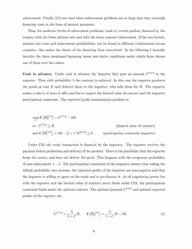
Cash in advance Under cash in advance the importer first pays an amount CCIA to the

exporter. Then with probability λ the contract is enforced. In this case the exporter produces

the goods at cost K and delivers them to the importer, who sells them for R. The exporter

makes a take it or leave it offer and has to respect the limited value of contract and the importer

participation constraint. The expected profit maximization problem is:

maxC

E[ΠCIAE

]= CCIA − λK,

s.t. CCIA ≤ R, (limited value of contract)

and E[ΠCIAI

]= λR− (1 + r∗)CCIA ≥ 0. (participation constraint importer)

Under CIA the trade transaction is financed by the importer. The exporter receives the

payment before production and delivery of the product. There is the possibility that the exporter

keeps the money and does not deliver the good. This happens with the exogenous probability

of non-enforcement 1− λ. The participation constraint of the importer assures that taking the

default probability into account, the expected profits of the importer are non-negative and thus

the importer is willing to agree on the trade and to pre-finance it. As all negotiation power lies

with the exporter and the limited value of contract never binds under CIA, the participation

constraint binds under the optimal contract. The optimal payment CCIA and optimal expected

profits of the exporter are:

CCIA =λ

1 + r∗R, E

[ΠCIAE

]=

λ

1 + r∗R− λK. (1)

8

Note that λ appears in the optimal payment CCIA. Thus the importer’s payment is dis-

counted by the probability of non-payment by the exporter. Under CIA production and delivery

only takes place with probability λ.

Open account Under open account first the exporter produces the goods at cost K and then

delivers them to the importer. Next, the importer sells the goods for R. With probability λ∗

the contract is enforced and the importer pays the amount COA to the exporter.

The profit maximization problem of the exporter is:

maxC

E[ΠOAE

]=

11 + r

(λ∗COA −K(1 + r)),

s.t. COA ≤ R, (limited value of contract)

and E[ΠOAI

]=

11 + r∗

(R− λ∗COA) ≥ 0, (participation constraint importer)

assuming that the exporter and importer discount profits with their local interest rates.18

Now, the exporter pre-finances the trade interaction. The importer receives the goods before

payment. With probability 1 − λ∗ the importer is not forced to pay the exporter. Due to the

limited value of contract constraint the maximum payment COA that is contractible is the sales

value of the product R. Under this maximum payment the exporter is not able to extract all

rents from the importer. Thus under open account the importer has positive ex-ante expected

profits. There is no contract that allows the exporter to extract all surplus.19 The optimal

payment amount COA and the optimal discounted expected exporter profits can be derived as:

COA = R, E[ΠOAE

]=

λ∗

1 + rR−K. (2)

Letter of credit Under LC the financial transaction is secured via a bank in the country of

the exporter and the importer, respectively. Under the assumption of no default at the bank

level, this completely resolves the enforcement problem at the individual contract level20. The18In order to be able to compare profits between CIA and OA they have to be discounted to the same time

period.19This is true for any finite upper bound on the contractible payment level. Without an upper bound any

change in enforcement probability could be offset by a proportional increase in COA. It is conceivable thoughthat courts would not enforce amounts too disconnected from the real value of the trade.

20It is conceivable that full enforcement at the banking level is more likely than at the firm level. As banks tendto have more long-term relationships, reputation building and repeated transactions ease enforcement betweenthem.

9

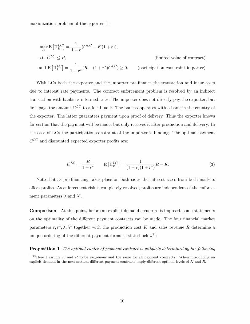
maximization problem of the exporter is:

maxC

E[ΠLCE

]=

11 + r

(CLC −K(1 + r)),

s.t. CLC ≤ R, (limited value of contract)

and E[ΠLCI

]=

11 + r∗

(R− (1 + r∗)CLC) ≥ 0. (participation constraint importer)

With LCs both the exporter and the importer pre-finance the transaction and incur costs

due to interest rate payments. The contract enforcement problem is resolved by an indirect

transaction with banks as intermediaries. The importer does not directly pay the exporter, but

first pays the amount CLC to a local bank. The bank cooperates with a bank in the country of

the exporter. The latter guarantees payment upon proof of delivery. Thus the exporter knows

for certain that the payment will be made, but only receives it after production and delivery. In

the case of LCs the participation constraint of the importer is binding. The optimal payment

CLC and discounted expected exporter profits are:

CLC =R

1 + r∗, E

[ΠLCE

]=

1(1 + r)(1 + r∗)

R−K. (3)

Note that as pre-financing takes place on both sides the interest rates from both markets

affect profits. As enforcement risk is completely resolved, profits are independent of the enforce-

ment parameters λ and λ∗.

Comparison At this point, before an explicit demand structure is imposed, some statements

on the optimality of the different payment contracts can be made. The four financial market

parameters r, r∗, λ, λ∗ together with the production cost K and sales revenue R determine a

unique ordering of the different payment forms as stated below21:

Proposition 1 The optimal choice of payment contract is uniquely determined by the following21Here I assume K and R to be exogenous and the same for all payment contracts. When introducing an

explicit demand in the next section, different payment contracts imply different optimal levels of K and R.

10

three conditions:

i) OA ≺ CIA⇐⇒ K

R<λ∗(1 + r∗)− λ(1 + r)(1 + r)(1 + r∗)(1− λ)

,

ii) OA ≺ LC ⇐⇒ λ∗(1 + r∗) > 1,

iii) LC ≺ CIA⇐⇒ K

R<

1− λ(1 + r)(1 + r)(1 + r∗)(1− λ)

.

Proof. Follows directly from comparing optimal discounted expected profits, Equations (1)-(3).

Proposition 1 summarizes the different effects of the parameters on expected profits under

the different financing forms. The usage of open account is increasing in enforcement abroad

λ∗ and decreasing in financing costs at home r. CIA is more likely to be used if enforcement

at home λ is strong and if financing costs abroad r∗ are high. LCs are used if enforcement is

relatively weak (low λ, λ∗) and if financing costs are relatively low (low r, r∗).

3 The trade model

In the following I introduce a CES demand structure that is standard in intra-industry trade

models. I analyze the effects of trade finance at the firm level in partial equilibrium. This allows

to derive predictions of the model in a trade framework that could be taken to the data.

3.1 Basic Setup

Preferences Assume the following preferences:

U = Qµq1−µ0 with Q =

(∫Ωq(ω)

σ−1σ dω

) σσ−1

. (4)

Q is a CES basket of a continuum of differentiated goods and q0 is a homogenous good. There

is a Cobb-Douglas utility function between the homogeneous good and the differentiated goods

implying constant shares of income spent on differentiated goods and the homogeneous good,

respectively. The demand for a single variety of the differentiated good has the standard form:

q(ω) = p(ω)−σP σQ.

11

ω denotes a variety of the differentiated goods. P =(∫ω∈Ω p(ω)1−σ)1−σ is the price index of the

optimal CES basket. σ > 1 is the elasticity of substitution between varieties and Q is the total

demand for differentiated goods.

Technology Labor is the only input factor. Firms in the homogenous goods sector face perfect

competition. They operate a constant returns to scale technology requiring one unit of labor per

unit of output. The homogenous good is freely traded. I only consider equilibria in which every

country produces the homogenous good. This equalizes wages, which I normalize to one making

the homogenous good the Numeraire. In the differentiated goods sector firms face monopolistic

competition. Each variety is produced by only one firm. There is a fixed cost of entry into

the market f . The production of one unit of the differentiated product requires a units of

labor input. Thus the total labor requirement of a firm operating and producing quantity q is

l(a) = f + aq. When selling a differentiated good abroad, a firm incurs iceberg type trade costs.

In order for one unit of a differentiated product to arrive in the destination country, τ > 1 units

have to be shipped.

3.2 Optimal behavior of firms

Differentiated sector Firms in the differentiated sector maximize their expected profits.

Given CES utility and monopolistic competition firms optimally do markup pricing. Domestic

prices, quantities and profits can be derived as:

pd =σ

σ − 1a, qd = (pd)

−σ P σQ, Πd = qd

[a

σ − 1

]. (5)

Next, I derive the optimal behavior of firms on the export market. Optimal profits under all

financing forms can be represented by the general expression:

E [Πx] = αR− βK.

This problem can be rewritten to E[Πx

]= E

[Πxα

]= R − β

αK. Maximizing the original

objective function E [Π] implies the same optimal decisions as maximizing the new function

E[Π]. This price setting problem is equivalent to the standard case with new per unit production

12

costs of βαa.

Thus the optimal export decision of a firm implies:

px =β

ατp∗d, E [qx] = Aτ1−σq∗d, E [Πx] = Aτ1−σΠ∗d, (6)

with A=ασβ1−σ.22

The finance profit factor A fully summarizes the effects of payment contracts on expected

profits and expected quantities at the factory gate. A = 1 corresponds to no financing frictions,

which would be the case if r = r∗ = 0 and λ = λ∗ = 1. Then expected profits are the same as

in the standard model. Note that the parameters α and β enter the problem in a multiplicative

form with the value of exports. Thus the model endogenizes some of the variable trade costs of

trade arising from financing costs and the enforcement problem.23

Now that the explicit demand structure is defined, I can derive new conditions for the

optimal financing forms. The profits and quantities under financing form 1 are larger than

under financing form 2 iff:

A1 > A2.

Plugging in the different values for α and β delivers:24

Corollary 1 The optimal choice of payment contract is uniquely determined by the following

three conditions:

i) OA ≺ CIA⇐⇒ (λ∗)σ

λ

(1 + r∗

1 + r

)σ> 1,

ii) OA ≺ LC ⇐⇒ λ∗(1 + r∗) > 1 (as before),

iii) LC ≺ CIA⇐⇒ λ(1 + r)σ < 1.

22E [qx] is the expected quantity at the factory gate, i.e. including iceberg trade costs and taking into accountthat under CIA only a fraction λ of export contracts is enforced. That is: E [qx] = τβ(p∗x)−σ(P ∗)σQ∗.

23It would be interesting to combine the value-dependant variable costs introduced in this model with someunit-dependent transport costs.

24In the case of CIA the parameters are: α = λ1+r∗ and β = λ, under OA α = λ∗

1+rand β = 1 and und LC

α = 1(1+r)(1+r∗)

and β = 1

13

Proof. These conditions follow directly from a comparison of expected profits.25

The expressions simplify, but the same factors as in the general case can be identified: CIA

is more likely to be used if enforcement at home λ is strong and financing costs abroad r∗ are

low. OA is more likely used if enforcement abroad λ∗ is strong and financing costs at home r∗

are low. LCs are used if enforcement is relatively weak (low λ, λ∗) and if financing costs are

relatively low (low r, r∗).

3.3 Payment Contract Switching

Optimal switching An exporter switches payment contract when this maximizes expected

profits. Maximizing expected profits is equivalent to maximizing expected quantities at the

factory gate. In this subsection I discuss how the ability to switch contracts allows a firm

to mitigate partially adverse effects from financial markets. First, note that for any financial

variable θ ∈ r, r∗, λ, λ∗ there is at least one payment contract under which expected profits,

revenues and quantities are independent of this variable. Thus if there is a deterioration of one

of these variables at some point a firm will switch its payment contract. There are also pairs of

financial variables of which some payment contracts are independent.

Thus there are cases when the possibility of a payment contract switch can at some point

completely mitigate any adverse effects on trade. However, there can be changes in several

financial variables for which there is no financing form that completely mitigates the effects.

Nevertheless, a switch of payment contract can reduce the impact of financial market changes.

Effects of contract switching In the following I illustrate these different cases with some

graphs for trade between firms in different countries.26

Figure 2 illustrates the difference between a change in only one financial variable, the effects

of which can be fully mitigated, and a simultaneous change in two financial variables, the negative

effects of which cannot be fully eliminated by switching contracts.25Prices and profits for the three financing forms are:

pCIA = (1 + r∗)τp∗d E[ΠCIAE

]=

(1

1 + r∗

)σλτ1−σΠ∗

d

pOA =1 + r

λ∗τp∗d E

[ΠOAE

]=

(λ∗

1 + r

)στ1−σΠ∗

d

pLC = (1 + r)(1 + r∗)τp∗d E[ΠLCE

]= ((1 + r)(1 + r∗))

−στ1−σΠ∗

d

26All graphs are calculated in partial equilibrium, i.e. keeping foreign demand fixed. In Section 4 the sameexperiments are studied under general equilibrium. For all graphs the following baseline calibration is used:1 + rN = 1.02, 1 + rS = 1.04, λN = 0.98, λS = 0.95.

14

Here figure 2

In the left graph, rN = 1.02 is constant and only the Southern interest rate varies. The initial

payment contract is Cash in Advance. When the interest rate in the South passes a threshold,

there is a switch of payment contract to Open Account. From that point on changes in the

Southern interest rate do not affect trade volumes. In the right graph, rN = rS − 0.02 is a

constant value below the southern interest rate. Initially both interest rates are low and a

Letter of Credit is used. When both interest rates increase beyond a certain point, there is a

switch to Cash in Advance. Note that the switch reduces the impact of the financial changes,

but cannot fully eliminate them.

A switch of payment contract takes place when the ordering of the finance profit factors A

changes. This is illustrated in Figure 3, which shows the values of profit factors in the experiment

discussed above for the different payment forms. Quantities depend only on the factor A specific

to the payment form actually used, which is the maximum of the three lines.

Here figure 3

Figure 4 illustrates the case where two financial parameters change and it is still possible to

fully eliminate effects on trade from some point onwards. Now enforcement in the South and in

the North and South are changed respectively.

Here figure 4

In the left graph, λN = 0.98 is constant and only the Southern enforcement probability changes.

For low values of enforcement, Cash in Advance is used. When the enforcement rate in the South

gets very close to the Northern one, then the payment contract is switched to Open Account in

order to profit from the lower interest rate in the North. In the right graph, λN = λS + 0.03 is a

constant value above the enforcement value in the South. For low values of enforcement, Letter

of Credit is chosen, which fully eliminates any effect of the enforcement probabilities on trade

quantities. For higher values of enforcement, there is a switch to Cash in Advance and trade

rises with enforcement in the North.

Effects of no contract switching in the short run The ability of an exporter to switch to

a different payment contract is important to optimally adjust to the changes in financial efficien-

cies and enforcement probabilities. When an exporter is not able to switch payment contracts

in the short run, this has an adverse affect on traded quantities and expected profits. This is

illustrated in Figure 5. In the example, interest rates are relatively low to begin with and a

Letter of Credit is used. Now suppose there is a change in the Northern interest rate. Then at

15

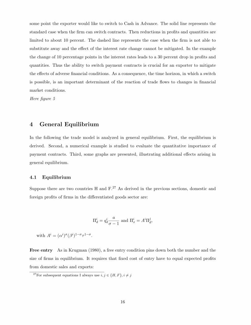
some point the exporter would like to switch to Cash in Advance. The solid line represents the

standard case when the firm can switch contracts. Then reductions in profits and quantities are

limited to about 10 percent. The dashed line represents the case when the firm is not able to

substitute away and the effect of the interest rate change cannot be mitigated. In the example

the change of 10 percentage points in the interest rates leads to a 30 percent drop in profits and

quantities. Thus the ability to switch payment contracts is crucial for an exporter to mitigate

the effects of adverse financial conditions. As a consequence, the time horizon, in which a switch

is possible, is an important determinant of the reaction of trade flows to changes in financial

market conditions.

Here figure 5

4 General Equilibrium

In the following the trade model is analyzed in general equilibrium. First, the equilibrium is

derived. Second, a numerical example is studied to evaluate the quantitative importance of

payment contracts. Third, some graphs are presented, illustrating additional effects arising in

general equilibrium.

4.1 Equilibrium

Suppose there are two countries H and F.27 As derived in the previous sections, domestic and

foreign profits of firms in the differentiated goods sector are:

Πid = qid

a

σ − 1and Πi

x = AiΠjd,

with Ai = (αi)σ(βi)1−στ1−σ.

Free entry As in Krugman (1980), a free entry condition pins down both the number and the

size of firms in equilibrium. It requires that fixed cost of entry have to equal expected profits

from domestic sales and exports:27For subsequent equations I always use i, j ∈ H,F, i 6= j

16

f = Πid + Πi

x.

Next, I combine the two equations resulting from free entry and solve for domestic quantities:28

qid =σ − 1a

f1−Ai

1−AiAj.

Export quantities at the factory gate are given by:

qix = Aiqjd =σ − 1a

fAi(1−Aj)1−AiAj

.

Note that due to the Cobb Douglas structure in preferences the expenditure share on differenti-

ated products is fixed. Thus output in the differentiated sector, measured in labor, is constant.

Taking partial derivatives allows to analyze effects of A on quantities:

∂qid∂Aj

= − ∂qix

∂Aj=σ − 1a

f(1−Ai)Ai

(1−AiAj)2> 0,

and∂qid∂Ai

= − ∂qix

∂Ai= −σ − 1

af

1−Aj

(1−AiAj)2< 0.

Lemma 1 In the two country trade model exported (domestic) quantities are

i) increasing (decreasing) in profit factor Ai,

ii) decreasing (increasing) in profit factor Aj.

Thus in the two country model domestic quantities are decreasing in the own export profit

parameter A and increasing in the foreign export parameter A∗. Due to the choice of payment

contracts all financial parameter r, r∗, λ, λ∗ can affect both A and A∗. Thus while the effect of the

profit parameters A and A∗ on quantities is unambiguous, no general result can be established

for the effect of the four financial parameters on traded and domestic quantities.

Total (expected) quantities at the factory gate are constant:29

28Plugging in the values derived for profits from before delivers:

f =a

σ − 1

[qid +Aiqjd

].

29Quantities are:

17

qi =σ − 1a

f.

Labor market clearing The number of firms in both countries is determined by labor market

clearing.30 Given the CD preferences, a constant fraction of labor is employed by the differen-

tiated sector:

LiQ = µLi.

Labor in the differentiated sector is used for entry and production:

LiQ = LiE + LiP = ni(f + aq).

From this the following result for the number of firms can be derived:

n =µLi

f + aq=µLi

σf.

4.2 Numerical Example

In the following, properties of the model are illustrated using a numerical example. The quan-

titative importance of payment contract switches is evaluated.

Country Types Suppose there are three types of countries. Type I has a very efficient fi-

nancial market and strong enforcement. Type II has a relatively efficient financial market, but

enforcement is weak. Type III has a less efficient financial market, but relatively strong enforce-

ment. The countries are characterized by the parameters in Table 1:

qi = qid + qjdAi.

Plugging in domestic quantities delivers total quantities per firm:

qi =σ − 1

af

1

1−ASAN[(1−AN ) + (1−AS)AN

].

The last expressions can be simplified to obtain the standard result as stated above.30For tractability, I assume that the positive expected profits of importers under Open Account do not enter the

demand for differentiated good. These profits occur under Open Account as only a share of importers fulfill thecontract and payment COA is limited to be smaller or equal to R. It would be interesting to analyze these ’informal’profits explicitly in the general equilibrium. This could be relevant for countries with very low enforcement rates.

18

here table 1

Optimal Contracts As shown before these country characteristics can be mapped uniquely

into the optimal choice of payment contract for each exporter-importer country combination.

The optimal payment contracts chosen are:

here table 2

The rows correspond to the country type of the exporter, the columns to the country type of

the importer. On the diagonal the countries are symmetric. In this case an exporter would

never choose OA as this is dominated by CIA. Thus given symmetric countries either CIA or

LC is chosen depending on the domestic interest rate and domestic enforcement. For trade

between countries of type II where enforcement is low, LC is chosen, whereas country I and III

choose CIA. Country type II has low enforcement. Therefore, its exporters choose contracts

that circumvent this problem, i.e. OA and LC. The main factor for the choice of an exporter in

a country of type III is the relatively high home interest rate. The only payment contract that

is independent of this interest rate is CIA, which is the dominant payment contract for trade

with all three types of trading partners. Given these payment contracts, traded quantities can

be calculated:

here table 3

To evaluate quantitatively the effects of the choice of payment contracts on trade, two exper-

iments are studied. First, the differences in trade volumes between the optimal contract and

the worst contract are calculated. Second, the differences in trade volumes between the optimal

contract and any of the three available contracts are calculated.31

Worst contracts The contracts that minimize quantities and profits for exporter-importer

pairs are:

here table 4

The percentage decreases in quantities relative to the optimal payment contracts are:

here table 5

If, for example, an exporter in a country of type I trading with an importer in country type II31For both experiments I assume that exporters in the home country are constrained, while exporters in the

country abroad choose the optimal payment contract. I do not report the reverse trade flows (from abroad tohome) here. Nevertheless, they have an impact on price levels and thus on traded quantities of home countryexporters.

19

would be forced to use OA instead of CIA, this would reduce the traded quantity by 49.4 percent.

The table shows that the choice of payment contract has a quantitatively important effect on

traded volumes. Furthermore, this effect is heterogeneous across country pairs. Some trade,

like trade between type I countries, does not depend very much on the payment contract in use.

Trade between countries of type II on the other hand, which have low enforcement, benefits

a lot from the ability of exporters to avoid OA. Note that, whether symmetric or asymmetric

countries trade with each other, is not a good predictor of potential losses from non-optimal

payment contracts. Which country-pair combinations profit most from a free choice of payment

contracts depends on the interaction of all four financial parameters as shown in the previous

sections.

The percentage decreases in traded quantities relative to the optimal contract if exporters

are forced to use one specific contract are:

here table 6

4.3 Graphical Illustrations

In the following, additional effects arising in the two country general equilibrium model are

discussed. The experiments shown in Figures 2 to 5 are repeated in Figures 6 to 8. The

dashed lines represent the previously discussed partial equilibrium responses. The solid lines

represent the full general equilibrium results. There are two new general equilibrium effects.

Changes in financial efficiency and enforcement affect the finance profit factor A of Northern

exporters and thus their prices and quantities. This has an effect on price level in the South and

thus affects the export decision of Northern exporters. A second effect arises from the Southern

exporters. Their finance profit factor is also affected by changes in the efficiency and enforcement

parameters, altering export quantities and prices and thus price levels. Furthermore, when

financial parameters change, exporters in the South might optimally switch payment contracts.

These switches have an impact on the Northern exporters through price levels, too. Note that

the switching decisions of Northern exporters is independent of general equilibrium effects as it

only depends on exogenous financial parameters.

Figure 6 illustrates changes in interest rates. It corresponds to Figure 2 in partial equilibrium.

In the left graph, Northern exporters switch from CIA to OA at the same point as before.

Now there is a new effect from a switch by exporters in the South, though. The vertical

20

solid line marks the threshold at which they switch their payment contract from LC to CIA in

order to substitute away from the rising Southern interest rate. Now with a further rise in r∗,

Northern exports become relatively more expensive. Thus exports fall steeper than in partial

equilibrium. At the vertical dashed line, the Northern exporters switch as well and all trade

becomes independent of the Southern interest rate.

In the right graph, when both Northern and Southern interest rates rise jointly, there is no

switch by Southern exporters who use CIA. The fall of Northern exports is less steep in general

equilibrium as also Southern exporters are affected by the changes in interest rates. Thus the

relative price of Northern exporters rises less quickly and trade decreases by less than in partial

equilibrium.

Here figure 6

Figure 7 illustrates changes in enforcement. It corresponds to Figure 4 in partial equilibrium.

In the left graph as before Northern exporters switch from CIA to OA. Exporters in the South

use CIA and do not switch. In the left part of the figure, the solid line is now decreasing as

Southern exporters become more competitive with a rise in λ∗, i.e. the relative price of North-

ern exporters rises and their quantities decrease. In the right graph, initially exporters in both

countries use a LC and then at some point switch to CIA. Southern exporters do so first as the

interest rate in the North is lower. From the point of the switch onwards, they become relatively

more competitive and quantities of Northern exporters decrease. This is the case until Northern

exporters themselves switch to CIA and their sales increase with the further rise of Northern

enforcement.

Here figure 7

Figure 8 illustrates the case of no contract switching in the short run. It corresponds to Fig-

ure 5 in partial equilibrium. As before, if they can do so in the short run, Northern exporters

switch from LC to CIA. Exporters in the South first use CIA and then later switch to OA.

After the Northern exporters switch contracts and before the Southern exporters change their

choice, all exporters use CIA. Then, only exporters in the South are affected by the increase

in the Northern interest rate. This makes Northern exporters relatively more competitive and

their exports rise. When Southern exporters switch as well, trade becomes independent of the

Northern interest rate. If exporters in the North cannot switch contracts, their exports decrease

in the whole range. First, when also exporters in the South are affected by the interest rate, the

decrease is relatively smaller. Then, when Southern exporters switch contracts and their sales

21

become independent of the Northern interest rate, the slope of the line representing trade gets

steeper and the competitiveness of Northern exporters deteriorates more quickly.

Here figure 8

5 Repeated Transactions

In the previous sections the relationship between an exporter and an importer consisted of only

one transaction. Often though, trade relationships are longer lasting, i.e. there is the possibility

that the two trading partners interact again in subsequent periods. Repeated transactions give

rise to a continuation value of a trade relationship, which makes the non-fulfillment of a contract

less desirable. In this section I introduce the possibility of repeated transactions between an

exporter and an importer and study under which conditions a simple trigger strategy can be

implemented to improve upon the equilibrium of the one shot game. I find that the ability

to sustain a trigger strategy equilibrium increases with enforcement probabilities and with the

survival probability of the trade relationship. Under CIA the ability also increases in the markupσσ−1 and iceberg trade costs τ .

Suppose that trade can happen more than once between two trading partners. Let γ denote

the probability that a given trade relationship can be continued in the next period. That is γ is

the the trade relationship survival rate. As before a match between an exporter and an importer

is analyzed. No new trading relationships are created, i.e. there are no outside options to trade

with another partner.32

CIA First, I analyze the case of Cash in Advance. Consider the following trigger strategy.

The importer pays the full revenue amount discounted by the interest rate, i.e. C = R1+r∗ . If

the exporter ever fails to deliver, the importer punishes by ending the trade relationship. The

exporter always pays the money and never runs away. The equilibrium exists if the exporter

has no incentive to deviate, i.e. to take the money and not deliver the good. Yet, even when

deviating, with probability λ the exporter is forced to fulfill the contract. That is, the higher

the enforcement probability at home, the less likely the exporter does profit from a deviation.

In order for the trigger strategy to be an equilibrium, the value of the relationship for32It would be an interesting extension to allow for the creation of new relationships via searching and matching.

This would increase the value of the outside option and make it more difficult to sustain a trigger strategyequilibrium.

22

the exporter VE has to be larger than the one period deviation payoff. The trigger strategy

equilibrium exists iff:

VE =∞∑n=0

(γ

1 + r

)n(C −K) =

C −K1− (γ/(1 + r))

> (1− λ)C.

Using CCIA = R1+r∗ this condition holds iff:33

σ

σ − 1τ

[1−

(1− γ

1 + r

)(1− λ)

]> 1

There are different factors, which make the condition more likely to hold. It holds more

likely for a higher λ. As the expected gain from a deviation decreases in domestic enforcement,

implementation of the trigger strategy is the easier, the better enforcement. Furthermore, the

trigger strategy equilibrium is easier to sustain when the ratio R/K increases, i.e. when revenues

are relatively large compared to production costs. This is the case when the markup and iceberg

trade costs are higher. Finally, the higher γ, the higher the value of the trade relationship, the

easier it is to implement the trigger strategy.34

OA Under OA the relevant deviation is by the importer. When OA is used an importer has

positive expected profits in the one shot game:

ΠOAI =

R(1− λ∗)1 + r∗

.

In a trigger strategy equilibrium the importer has to receive at least as large expected profits as in

the one shot game. The equilibrium considered is as follows: The importer always pays amount

C. If the importer ever fails to pay the amount, the exporter stops the relationship. First note

that for the importer to have positive expected profits, the payment C has to be strictly below

the revenues R for any λ∗ < 1. The amount C that makes the importer indifferent between

adhering to the trigger strategy equilibrium and deviating is characterized by:33

C −K > (1− (γ/(1 + r)))(1− λ)C ⇔ C

[1−

(1− γ

1 + r

)(1− λ)

]> K

Next use CCIA = R1+r∗ to get:

R

K

[1−

(1− γ

1 + r

)(1− λ)

]> (1 + r∗)

Plugging in RCIA

KCIA = (1 + r∗) σσ−1

τ delivers the result.34Note that so far only one specific trigger strategy is considered. In future research, it would be interesting to

look at a wider set of strategies featuring different forms of punishment.

23

VI =∞∑n=0

(γ

1 + r∗

)n(R− C1 + r∗

)=

R− C(1 + r∗)(1− (γ/(1 + r∗)))

=R(1− λ∗)

1 + r∗.

This condition corresponds to the equilibrium chosen by the exporter, who has all negotiation

power. It determines the highest incentive compatible C and thus maximizes expected profits

of the exporter. The maximum payment C is:

CTR,OA = R

[1−

(1− γ

1 + r∗

)(1− λ∗)

].

The amount increases in the survival probability γ and the enforcement probability abroad

λ∗. Under OA a trigger strategy always improves on the one shot game whenever γ > 0. To see

this note that the expected payment in the one shot game is λ∗R. The expected payment under

a trigger strategy with open account is CTR,OA. The latter is larger iff:

R

[1−

(1− γ

1 + r∗

)(1− λ∗)

]> λ∗R.

This condition can be simplified to obtain γ > 0.35

LC versus other Payment Contracts As shown above, under the discussed conditions,

trigger strategies can improve upon one shot equilibria in the cases of CIA and OA. A LC

on the other hand already resolves all enforcement problems. Trigger strategies can thus not

improve upon the one shot equilibrium in this case. As a result, the introduction of trigger

strategies and repeated transactions makes CIA and OA more attractive while leaving the LC

unaffected, implying a worsening of the relative attractiveness of LCs. This is especially the case

when transaction horizons are long, characterized by high relationship survival probabilities γ,

and when enforcement probabilities λ and λ∗ are high. Thus long lasting relationships and

trade between countries with high enforcement imply a higher usage of trigger strategies and

less reliance on the LC.

Levchenko, Lewis, and Tesar (2009) find that trade credit intensive industries are not more

strongly affected by the financial crisis than others. This finding might be explained by the

presence of both one shot equilibria and repeated games equilibria in the data. Inter-firm trade

credit usually corresponds to CIA and OA. The model predicts that these two payment contracts35

λ∗ < 1− γ

1 + r∗(1− λ∗)⇔ 1 > 1− γ

1 + r∗

24

are used more intensively when trigger strategies can be implemented more easily. In a successful

trigger strategy equilibrium, only one financial variable affects the traded quantities, i.e. r∗ for

CIA and r for OA. Thus trade credit intensive industries, which use relatively more CIA and

OA, should be less affected by shocks to financial markets than industries that rely more on the

LC.36

6 Implications of Endogenous Payment Contracts

6.1 Financial and Economic Turmoil

In the following I analyze the effects of different forms of financial and economic turmoil on

trade profits and quantities.

Enforcement and Country level risk Suppose that the enforcement probability λ is a

combination of national risk and individual firm level risk. National risk corresponds to risk

of expropriation, risk of sovereign or bank level default while individual risk is the probability

that a specific contract is enforced. The important difference between the two is that banks

are only affected by national risk. Before, a Letter of Credit could fully resolve the problem of

enforcement for the exporter. Now, with national risk, the only way to fully mitigate changes in

λ is to switch to Open Account. Let overall risk be the product of national risk and individual

contract risk:

λ = λNλI

Given this, trade finance reacts differently depending on the source of the enforcement prob-

lems. An decrease of enforcement at the contract level in the exporter’s country implies a shift

towards Open Account or Letter of Credit. A decrease in the importer’s country contract en-

forcement leads to a shift towards Cash in Advance and Letter of Credit. An increase in national

risk, however, cannot be solved by switching to a Letter of Credit. In this case an exporter can

only switch to Open Account and an importer can only switch to a Cash in Advance to fully

eliminate the effect of domestic enforcement problems. In the following I discuss different types

of turmoil that can be observed in reality and elaborate on some predictions of the model.36Trade using a trigger strategy is less affected by changes in financial parameters as long as the trigger strategy

equilibrium can be sustained, i.e. as long as changes in parameters to not lead to a breakdown of the triggerstrategy equilibrium.

25

Interest rate changes There are two potential sources of interest rate changes. First, due

to events that might take place outside the two trading countries, the world interest rate rw

can change, moving both interest rates simultaneously. Second, there can be some problems of

banks in one or both of the countries so that their efficiency parameters ϕi change, which affects

interest rates.37 The effect of these changes crucially depends on the time horizon in which firms

are able to switch their payment contracts. If they are fully flexible in their choice of payment

contracts, then the effects of interest rates changes are captured by Figure 2 as discussed above.

If firms are not flexible in the short run, the effects of interest rate changes might be stronger as

shown in Figure 5. If an exporter can change the payment contract in the time horizon studied,

then a unilateral change in the interest rate can, from some point on, be fully mitigated while a

change in both interest rates cannot. If there is a short run inability to switch contracts, then

we should not observe a differential effect of unilateral and multilateral changes in interest rates.

Contract level enforcement changes As introduced above there are enforcement problems

at the national and at the contract level. From these two, the national risk seems to be more

susceptible to turmoil. The individual contract enforcement is mainly determined by legal

institutional factors, which should in general not change in the short run.38 Yet, perceived

national risk like sovereign default or expropriation probabilities can change relatively quickly.

As discussed above, national risk cannot be mitigated by a Letter of Credit. Thus the only way

two trading partners can react to a deterioration in national risk in one of the two countries,

is to switch to the one contract that is not affected by this change: Open Account in case of a

deterioration in the exporter country and Cash in Advance in case of a worsening in the importer

country. Note, though, that this depends on the effect of changes in national risk on the interest

rate in the affected country. An increase in sovereign default could imply a proportional increase

in the national interest rate. That is, the risk free interest rate would then be scaled up by the

national risk. In this case no contract switching is possible to mitigate the effect. However,

any deviations from a proportional change in interest rates to changes in national risk allow

improvements through the choice of the optimal payment contract.37For details on rw and ϕi see the interest rate model in Appendix B.38If one would extend the individual contract enforcement by factors changing expected firm level insolvency

and illiquidity this would be different. Then, an economic crisis in a country could change contract fulfillmentexpectations at the firm level.

26

6.2 Trade Patterns

One aspect of trade that has been analyzed are differences in trade flows and trade volumes

between developed countries, between developed and developing countries and between develop-

ing countries. Taking into account that for trade both the financial conditions in the importer

and exporter country are relevant can help explain differences in trade patterns. A model that

looks at exporter financial markets only can e.g. not predict differences between South-South

and South-North trade as a result of financial conditions. All differences in such a framework

would be attributed to the demand side of trade. The new feature of my model, namely, that

the importer’s financial market and enforcement conditions matter, leads to the following two

propositions about trade volumes, export participation and importing country conditions:

Intensive margin

Proposition 2 For given domestic financial conditions r, λ and foreign demand conditions

P ∗ and Q∗, exports of a firm increase in foreign financial market conditions.

i) strictly if both r∗ decreases and λ∗ increases

ii) weakly if r∗ decreases or λ∗ increases

Proof. See Appendix A.

Exports of a country increase if the financial conditions in the country it is exporting to

improve. Thus, in order to predict trade flows, it is not sufficient to look at financial market

conditions in the country of the exporter alone, but one has to take into account the conditions in

both countries jointly. Analyzing payment contracts allows to understand how these conditions

interact and influence trade quantities.

Extensive margin Similar effects arise in a model with an extensive margin, where firms

decide whether to export or not to another country. To see this suppose for this paragraph that

there is a fixed cost fx of serving a foreign market, which has to be incurred by any firm which

wants to export. Then a firm will only export if the expected profits from entering the foreign

market are at least as large as the fixed cost that have to be incurred. Suppose that the fixed

cost can be financed without any additional financial problems. Then:

Proposition 3 For given domestic financial conditions r, λ and foreign demand conditions

P ∗ and Q∗, a firm is more likely to export if foreign financial market conditions are better.

27

i) strictly if both r∗ decreases and λ∗ increases

ii) weakly if r∗ decreases or λ∗ increases

Proof. See Appendix A.

Not only do trade volumes depend on the conditions in financial markets in the countries of

the exporter and the importer, but also the decision of firms to export, the extensive margin.

That is, the probability of exporting cannot be fully predicted by conditions in the financial

market of the exporter. Conditions in the financial market of the importer play a role, too.

6.3 FOB Prices

Given per unit cost a and iceberg transportation costs τ , different payment contracts imply

different FOB prices. To see this, note that from before the agreed on payment amounts C

differ by payment contract, i.e.:

CCIA =λ

1 + r∗RCIA, COA = ROA, CLC =

RLC

1 + r∗.

R is the amount of sales revenues in the importing country when trade takes place:

R =(β

ατ

)1−σr∗d.

The following payment amounts corresponding to FOB prices can be derived:

CCIA = λ(1 + r∗)−σ r, COA = (λ∗)σ−1(1 + r)1−σ r, CLC = (1 + r)1−σ(1 + r∗)−σ r,

with r = τ1−σr∗d.

From this it can be seen that the amounts specified to be payed for the traded goods vary

with financial market parameters in a systematic way. Depending on the payment form used

financial parameters affect FOB prices differentially. In an empirical analysis of FOB price data

it might thus be relevant to control for differences in payment contracts. Estimates regarding

FOB prices and financial indicators might otherwise be biased.

28

7 Conclusions

In this paper I propose a new theory explicitly modeling the choice of different payment con-

tracts in international trade. I analyze the trade-offs taken into account by an exporter choosing

between these different forms of payment, determined by enforcement probabilities and financ-

ing costs. The model shows that the choice of payment contracts is quantitatively important.

Financing decisions of trade transactions are driven by factors in the financial markets of the

exporter and the importer. The ability to freely choose and switch between payment contracts

is central for firms to adapt to different constellations of financial conditions in different country

pairs and over time. Limiting this choice can reduce traded quantities significantly, increase

prices, and reduce the ability of exporters to react to short term fluctuations in financial condi-

tions.

The model maps enforcement probabilities and financial market efficiencies of an exporter-

importer country pair into an optimal payment contract. In a richer model that could be brought

to the data one might want to include extensions concerning heterogeneity both in the firm and

in the product dimension. Product differences could imply different degrees of enforceability

in court or different time horizons of trade relationships (high or low γ). Firm differences in

size could affect relative negotiation power between the exporter and the importer, the ability to

enforce contracts in court, the ability to punish deviations from a trigger strategy and the ability

to switch contracts in the face of fixed costs. Another extension would be to explicitly introduce

currencies and to study the interaction of the payment contract decision with exchange rate

risk. This would give a suitable framework to study different aspects: first, which new effects

arise from payment contracts for the optimal decision in which currency to price exports, and

second, how this affects the transmission mechanism of international shocks.

There is little data available on the usage of the different payment contracts across countries,

firms and time. To assess the model empirically, available firm level data, that does not contain

direct evidence on payment contracts, could be used to test predictions of the model. Further-

more, a new data set on payment contracts could be built to directly test for determinants of

the choice of payment contracts.

29

References

Amiti, Mary, and David E. Weinstein, 2009, Exports and Financial Shocks, mimeo Federal

Reserve Bank of New York and Columbia University.

Auboin, Marc, 2007, Boosting Trade Finance in Developing Countries: What Link with the

WTO?, Wto staff working papers World Trade Organization.

Auboin, Marc, and Moritz Meier-Ewert, 2003, Improving the Availability of Trade Finance

during Financial Crises, Wto discussion papers World Trade Organization.

Baltensperger, Ernst, and Nils Herger, 2007, Exporting against Risk? Theory and Evidence

from Public Export Insurance Schemes in OECD Countries, University of Berne, mimeo.

Beck, Thorsten, 2002, Financial Development and International Trade: Is there a Link?, Journal

of International Economics 57, 107–131.

Beck, Thorsten, 2003, Financial Dependence and International Trade, Review of International

Economics 11, 296–316.

Bellone, Flora, Patrick Musso, Lionel Nesta, and Stefano Schiavo, 2008, Financial Constraints

as a Barrier to Export Participation, Documents de Travail de l’OFCE 2008-29 Observatoire

Francais des Conjonctures Economiques (OFCE).

Berman, Nicolas, and Jerome Hericourt, 2008, Financial Factors and the Margins of Trade:

Evidence from Cross-Country Firm-Level Data, Universite Paris 1 Pantheon-Sorbonne (post-

print and working papers) HAL.

Berman, Nicolas, and Philippe Martin, 2009, The Vulnerability of Sub-Saharan Africa to the

Financial Crisis: The Case of Trade, mimeo.

Berthou, Antoine, 2007, Credit Constraints and Zero Trade Flows: The Role of Financial De-

velopment, mimeo.

Berthou, Antoine, 2008, The Distorted Effect of Financial Development on International Trade

Flows, mimeo.

Biais, Bruno, and Christian Gollier, 1997, Trade Credit and Credit Rationing, Review of Finan-

cial Studies 10, 903–37.

30

Burkart, Mike, and Tore Ellingsen, 2004, In-Kind Finance: A Theory of Trade Credit, American

Economic Review 94, 569–590.

Chaney, Thomas, 2005, Liquidity Constrained Exporters, Working paper, University of Chicago.

Chauffour, Jean-Pierre, and Thomas Farole, 2009, Trade Finance In Crisis, Research working

papers World Bank.

Cunat, Vicente, 2007, Trade Credit: Suppliers as Debt Collectors and Insurance Providers, The

Review of Financial Studies 20, 491–527.

Djankov, Simeon, Caroline Freund, and Cong S. Pham, 2006, Trading on time, Policy Research

Working Paper Series 3909 The World Bank.

Dorsey, Thomas, 2009, Trade Finance Stumbles, Finance and Development 46.

Espanol, Paula, 2007, Exports, Sunk Costs and Financial Restrictions in Argentina during the

1990s, PSE Working Papers 2007-01 PSE.

Fabbri, Daniela, and Anna Maria Cristina Menichini, forthcoming, Trade Credit, Collateral

Liquidation and Borrowing Constraints, Journal of Financial Economics.

Greenaway, David, Alessandra Guariglia, and Richard Kneller, 2007, Financial Factors and

Exporting Decisions, Journal of International Economics 73, 377–395.

Helpman, Elhanan, 2006, Trade, FDI, and the Organization of Firms, Journal of Economic

Literature 44, 589–630.

Helpman, Elhanan, Marc Melitz, and Yona Rubinstein, 2008, Estimating Trade Flows: Trading

Partners and Trading Volumes, The Quarterly Journal of Economics 123, 441–487.

Hummels, David, 2001, Time as a Trade Barrier, Gtap working papers Center for Global Trade

Analysis, Department of Agricultural Economics, Purdue University.

Humphrey, John, 2009, Are Exporters in Africa Facing Reduced Availability of Trade Finance,

Institute of Development Studies, mimeo.

Iacovone, Leonardo, and Veronika Zavacka, 2009, Banking Crises And Exports, Policy research

working paper series The World Bank.

31

ICC, 2009, Rethinking Trade Finance 2009: An ICC Global Survey, ICC Banking Commission

Market Intelligence Report International Chamber of Commerce.

IMF, 2009, Sustaining the Recovery, World Economic Outlook International Monetary Fund.

Kletzer, Kenneth, and Pranab Bardhan, 1987, Credit Markets and Patterns of International

Trade, Journal of Development Economics 27, 57–70.

Krugman, Paul, 1980, Scale Economies, Product Differentiation, and the Pattern of Trade,

American Economic Review 70, 950–59.

Levchenko, Andrei A., Logan Lewis, and Linda L. Tesar, 2009, The Collapse of International

Trade During the 2008-2009 Crisis: In Search of the Smoking Gun, Discussion papers Univer-

sity of Michigan.

Manova, Kalina, 2008, Credit Constraints, Heterogeneous Firms, and International Trade,

NBER Working Papers 14531 National Bureau of Economic Research, Inc.

Matsuyama, Kiminori, 2005, Credit Market Imperfections and Patterns of International Trade

and Capital Flows, Journal of the European Economic Association 3, 714–723.

Melitz, Marc J., 2003, The Impact of Trade on Intra-Industry Reallocations and Aggregate

Industry Productivity, Econometrica 71, 1695–1725.

Petersen, Mitchell A, and Raghuram G Rajan, 1997, Trade Credit: Theories and Evidence,

Review of Financial Studies 10, 661–91.

Ronci, Marcio Valerio, 2004, Trade Finance and Trade Flows: Panel Data Evidence from 10

Crises, Imf working papers International Monetary Fund.

Stephens, Malcolm, 1998, Export Credit Agencies, Trade Finance and South East Asia, IMF

Working Papers 98/175 International Monetary Fund.

Stiebale, Joel, 2008, Do Financial Constraints Matter for Foreign Market Entry? A Firm-Level

Examination, Ruhr Economic Papers 0051 Rheinisch-Westfalisches Institut fur Wirtschafts-

forschung, Ruhr-Universitat Bochum, Universitat Dortmund, Universitat Duisburg-Essen.

Suwantaradon, Ruanjai, 2008, Financial Frictions and International Trade, University of Min-

nesota, mimeo.

32

Svaleryd, Helena, and Jonas Vlachos, 2005, Financial Markets, the Pattern of Industrial Special-

ization and Comparative Advantage: Evidence from OECD Countries, European Economic

Review 49, 113–144.

U.S. Department of Commerce, 2008, Trade Finance Guide, Working paper, International Trade

Administration.

Wilner, Benjamin S., 2000, The Exploitation of Relationships in Financial Distress: The Case

of Trade Credit, Journal of Finance 55, 153–178.

Zia, Bilal H., 2008, Export Incentives, Financial Constraints, and the (Mis)Allocation of Credit:

Micro-Level Evidence from Subsidized Export Loans, Journal of Financial Economics 87,

498–527.

33

A Proofs

Proposition 1 Proof. The statement is true for trade measured both in expected quantities

and in expected revenues at factory gate. Note that:

E [qx] = Aτ1−σq∗d = ασβ1−στ1−σq∗d

and

E [rx] =βτ

αAτ1−σr∗d = ασ−1β2−στ2−σr∗d

Taking partial derivatives delivers the following signs for A = ασβ1−σ:

CIA OA LC

A = ασβ1−σ (1 + r∗)−σλ (1 + r)−σ(λ∗)σ ((1 + r)(1 + r∗))−σ

∂A/∂r∗ − 0 −

∂A/∂λ∗ 0 + 0

As σ > 1 the expression for revenues ασ−1β2−σ delivers the same signs:

CIA OA LC

ασ−1β2−σ (1 + r∗)1−σλ (1 + r)1−σ(λ∗)σ−1 ((1 + r)(1 + r∗))1−σ

∂A/∂r∗ − 0 −

∂A/∂λ∗ 0 + 0

If r∗ decreases, both quantities and revenues increase under CIA and LC. If λ∗ increases,

quantities and revenues increase under OA.

Proposition 2 Proof. The extensive margin is determined solely by expected profits. Thus

it is sufficient to consider expected profits.

Note that:

E [Πx] = Aτ1−σΠ∗d = ασβ1−στ1−σΠ∗d

Thus profits are monotonously increasing in A. This combined with the partial derivatives

above proves Proposition 2.

34

B Interest rates

Suppose the importer and the exporter are in a small open economy and take the world interest

rate rw as given.In both countries there is a competitive sector of financial intermediation. Due

to technological and legal differences, the efficiency of the intermediation technology of banks in

different countries can differ. The intermediation technology displays constant returns to scale.

Let ϕi ≤ 1 be the efficiency of banks in country i for handling transactions, such that the cost of

lending one unit is 1/ϕi. Zero profit implies that the interest rate of a country charged to a firm

is ri = rw

ϕi. Thus both interest rates change with changes in rw. Furthermore, the interest rate

of a country changes with the efficiency parameter ϕ. This parameter captures both short - and

long-run effects. When there is financial turmoil in a single country and the domestic interest

rate rises, this is captured by a change in ϕ in that country.

When extending the model to the two types of enforcement problems, national and contract

level, the interest rate in a country will likely react to the former, i.e. the risk free world interest

rate will most likely be scaled up, reflecting national default risk. Let γ be the transmission factor

measuring the effect of changes in national risk on the local interest rate. That is, ri = rw

(λN )γϕi.

If γ = 0, then national risk has no effect on the interest rate. If on the other hand γ = 1, the

interest rate perfectly adjusts to any changes in national risk.

C Tables

Table 1: Country Types

Country Type I II IIIλ 0.99 0.85 0.97

1 + r 1.02 1.03 1.08

Table 2: Optimal Payment Contracts

from / to I II IIII CIA CIA OAII OA LC OAIII CIA CIA CIA

35

Table 3: Traded Quantities

Country I II IIII 2.94 2.9 2.6II 2.76 2.64 2.53III 3.02 2.93 2.45

Table 4: Worst Payment Contracts

from / to I II IIII LC OA LCII CIA OA CIAIII LC OA LC

Table 5: Optimal vs. Worst Payment Contract, percentage changes of quantities

from / to I II IIII -8.0 -49.4 -19.4II -9.3 -44.6 -23.2III -27.4 -59.2 -26.3

Table 6: Optimal vs. Only 1 Payment Contract, percentage changes of quantities

Only CIA Only OA Only LCfrom / to I II III I II III I II III

I 0 0 -12.8 -3.6 -49.4 0 -8.0 -7.8 -19.4II -9.3 -4.9 -23.2 0 -44.6 0 -4.5 0 -19.2III 0 0 0 -24.1 -59.2 -9.7 -27.4 -27.1 -26.3

36

D Figures

48% 45% 42%

33% 35%36%

19% 20% 22%

Oct '07 Oct '08 Jan '09

Cash-in-Advance Transactions

Bank-IntermediatedTransactionsOpen Account Transactions

Figure 1: Source: IMF World Economic Outlook

Figure 2: The effect of a change in interest rates on North-South trade flows. Solid line: tradedquantities. Vertical dashed line: change of payment contract.

37

Figure 3: The effect of a change in interest rates on the finance profit factor A. Vertical dashedline: change of payment contract.

Figure 4: The effect of a change of enforcement probabilities on North-South Trade flows. Solidline: traded quantities. Vertical dashed line: change of payment contract.

Figure 5: Percentage effect of a change in the interest rate in the North on North-South tradeflows with and without payment contract change. Dashed line: trade change with contractchange. Solid line top: trade change without contract change. Vertical dashed line: change ofpayment contract.

38

Figure 6: The effect of a change in interest rates on North-South trade flows, GE versus PE.Vertical dashed line: change of contract foreign exporter. Vertical solid line: change of contractdomestic exporter. Solid line: traded quantities general equilibrium. Dashed line: tradedquantities partial equilibrium.

Figure 7: The effect of a change of enforcement probabilities on North-South trade flows, GEversus PE. Vertical dashed line: change of contract foreign exporter. Vertical solid line: changeof contract domestic exporter. Solid line: traded quantities general equilibrium. Dashed line:traded quantities partial equilibrium.

39

Figure 8: Percentage effect of a change in the interest rate in the North on North-South tradeflows with and without payment contract change in general equilibrium. Vertical dashed line:change of contract foreign exporter. Vertical solid line: change of contract domestic exporter.Dashed line: trade change with contract change. Solid line: trade change without contractchange.

40