Towards an Algorithmic Realization of Nash’s Embedding Theorem

Nakul VermaCSE, UC San Diego

naverma@cs.ucsd.edu

Abstract

It is well known from differential geometry that ann-dimensional Riemannian manifold can be iso-metrically embedded in a Euclidean space of dimension2n+1 [Nas54]. Though the proof by Nashis intuitive, it is not clear whether such a construction is achievable by an algorithm that only hasaccess to a finite-size sample from the manifold. In this paper, we study Nash’s construction anddevelop two algorithms for embedding a fairly general classof n-dimensional Riemannian mani-folds (initially residing inRD) into R

k (wherek only depends on some key manifold properties,such as its intrinsic dimension, its volume, and its curvature) that approximately preserves geodesicdistances between all pairs of points. The first algorithm wepropose is computationally fast andembeds the given manifold approximately isometrically into aboutO(2cn) dimensions (wherec isan absolute constant). The second algorithm, although computationally more involved, attempts tominimize the dimension of the target space and (approximately isometrically) embeds the manifoldin aboutO(n) dimensions.

1 Introduction

Finding low-dimensional representations of manifolds hasproven to be an important task in data analysis anddata visualization. Typically, one wants a low-dimensional embedding to reduce computational costs whilemaintaining relevant information in the data. For many learning tasks, distances between data-points serve asan important approximation to gauge similarity between theobservations. Thus, it comes as no surprise thatdistance-preserving orisometricembeddings are popular.

The problem of isometrically embedding a differentiable manifold into a low dimensional Euclideanspace has received considerable attention from the differential geometry community and, more recently, fromthe manifold learning community. The classic results by Nash [Nas54, Nas56] and Kuiper [Kui55] show thatany compact Riemannian manifold of dimensionn can be isometricallyC1-embedded1 in Euclidean space ofdimension2n+ 1, andC∞-embedded in dimensionO(n2) (see [HH06] for an excellent reference). Thoughthese results are theoretically appealing, they rely on delicate handling of metric tensors and solving a systemof PDEs, making their constructions difficult to compute by adiscrete algorithm.

On the algorithmic front, researchers in the manifold learning community have devised a number ofspectral algorithms for finding low-dimensional representations of manifold data [TdSL00, RS00, BN03,DG03, WS04]. These algorithms are often successful in unravelling non-linear manifold structure fromsamples, but lack rigorous guarantees that isometry will bepreserved for unseen data.

Recently, Baraniuk and Wakin [BW07] and Clarkson [Cla07] showed that one can achieve approximateisometry via the technique of random projections. It turns out that projecting ann-dimensional manifold(initially residing inRD) into a sufficiently high dimensional random subspace is enough to approximatelypreserveall pairwise distances. Interestingly, this linear embeddingguarantees to preserve both the ambientEuclidean distances as well as the geodesic distances between all pairs of points on the manifold withouteven looking at the samples from the manifold. Such a strong result comes at the cost of the dimensionof the embedded space. To get(1 ± ǫ)-isometry2, for instance, Baraniuk and Wakin [BW07] show thata target dimension of size aboutO

(nǫ2 log

V Dτ

)is sufficient, whereV is then-dimensional volume of the

manifold andτ is a global bound on the curvature. This result was sharpenedby Clarkson [Cla07] by

1A Ck-embedding of a smooth manifoldM is an embedding ofM that hask continuous derivatives.2A (1± ǫ)-isometry means that all distances are within a multiplicative factor of(1± ǫ).

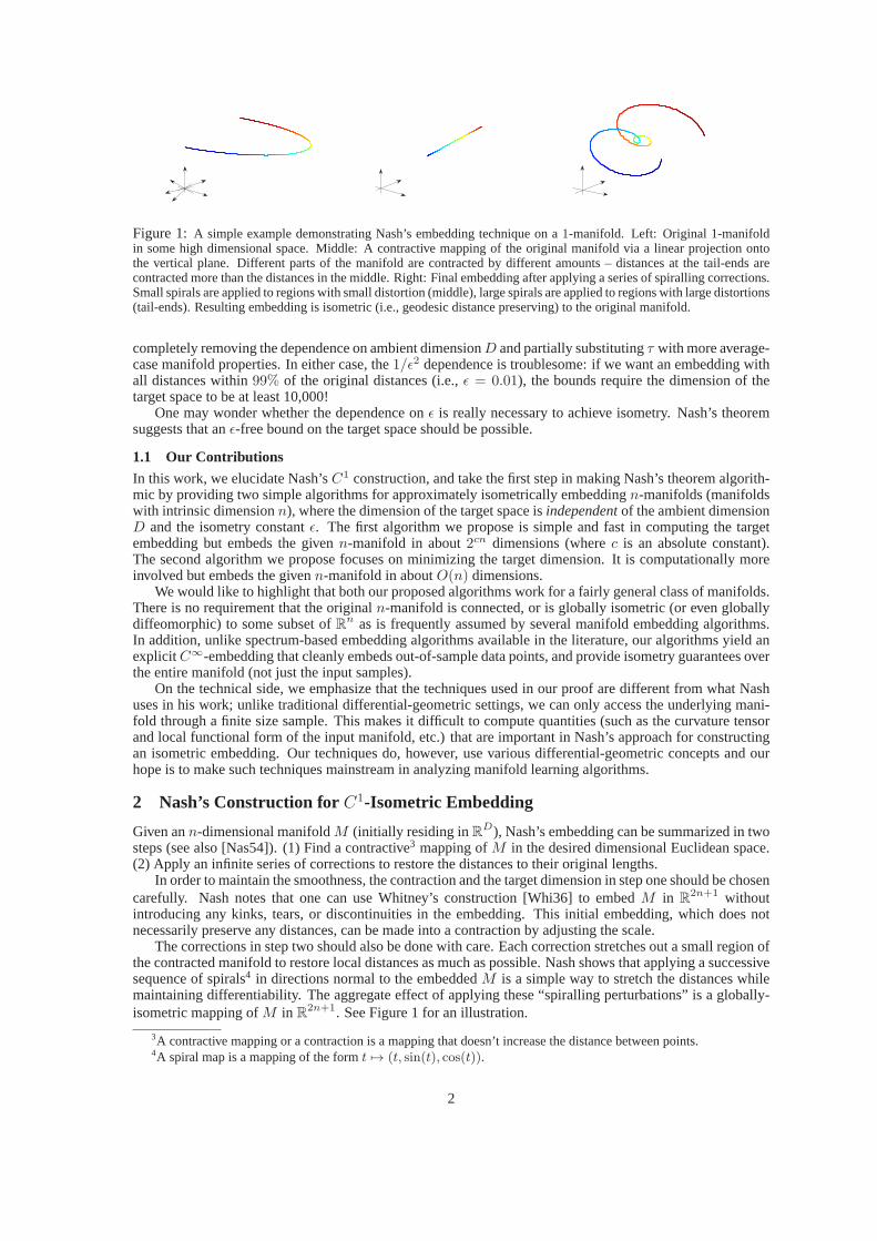
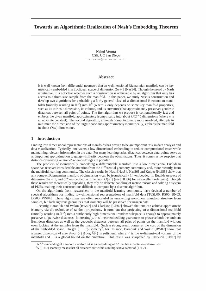
Figure 1: A simple example demonstrating Nash’s embedding technique on a1-manifold. Left: Original 1-manifoldin some high dimensional space. Middle: A contractive mapping of the original manifold via a linear projection ontothe vertical plane. Different parts of the manifold are contracted by different amounts – distances at the tail-ends arecontracted more than the distances in the middle. Right: Final embedding after applying a series of spiralling corrections.Small spirals are applied to regions with small distortion (middle), large spirals are applied to regions with large distortions(tail-ends). Resulting embedding is isometric (i.e., geodesic distance preserving) to the original manifold.

completely removing the dependence on ambient dimensionD and partially substitutingτ with more average-case manifold properties. In either case, the1/ǫ2 dependence is troublesome: if we want an embedding withall distances within99% of the original distances (i.e.,ǫ = 0.01), the bounds require the dimension of thetarget space to be at least 10,000!

One may wonder whether the dependence onǫ is really necessary to achieve isometry. Nash’s theoremsuggests that anǫ-free bound on the target space should be possible.

1.1 Our Contributions

In this work, we elucidate Nash’sC1 construction, and take the first step in making Nash’s theorem algorith-mic by providing two simple algorithms for approximately isometrically embeddingn-manifolds (manifoldswith intrinsic dimensionn), where the dimension of the target space isindependentof the ambient dimensionD and the isometry constantǫ. The first algorithm we propose is simple and fast in computing the targetembedding but embeds the givenn-manifold in about2cn dimensions (wherec is an absolute constant).The second algorithm we propose focuses on minimizing the target dimension. It is computationally moreinvolved but embeds the givenn-manifold in aboutO(n) dimensions.

We would like to highlight that both our proposed algorithmswork for a fairly general class of manifolds.There is no requirement that the originaln-manifold is connected, or is globally isometric (or even globallydiffeomorphic) to some subset ofRn as is frequently assumed by several manifold embedding algorithms.In addition, unlike spectrum-based embedding algorithms available in the literature, our algorithms yield anexplicitC∞-embedding that cleanly embeds out-of-sample data points,and provide isometry guarantees overthe entire manifold (not just the input samples).

On the technical side, we emphasize that the techniques usedin our proof are different from what Nashuses in his work; unlike traditional differential-geometric settings, we can only access the underlying mani-fold through a finite size sample. This makes it difficult to compute quantities (such as the curvature tensorand local functional form of the input manifold, etc.) that are important in Nash’s approach for constructingan isometric embedding. Our techniques do, however, use various differential-geometric concepts and ourhope is to make such techniques mainstream in analyzing manifold learning algorithms.

2 Nash’s Construction forC1-Isometric Embedding

Given ann-dimensional manifoldM (initially residing inRD), Nash’s embedding can be summarized in twosteps (see also [Nas54]). (1) Find a contractive3 mapping ofM in the desired dimensional Euclidean space.(2) Apply an infinite series of corrections to restore the distances to their original lengths.

In order to maintain the smoothness, the contraction and thetarget dimension in step one should be chosencarefully. Nash notes that one can use Whitney’s construction [Whi36] to embedM in R

2n+1 withoutintroducing any kinks, tears, or discontinuities in the embedding. This initial embedding, which does notnecessarily preserve any distances, can be made into a contraction by adjusting the scale.

The corrections in step two should also be done with care. Each correction stretches out a small region ofthe contracted manifold to restore local distances as much as possible. Nash shows that applying a successivesequence of spirals4 in directions normal to the embeddedM is a simple way to stretch the distances whilemaintaining differentiability. The aggregate effect of applying these “spiralling perturbations” is a globally-isometric mapping ofM in R

2n+1. See Figure 1 for an illustration.

3A contractive mapping or a contraction is a mapping that doesn’t increase the distance between points.4A spiral map is a mapping of the formt 7→ (t, sin(t), cos(t)).

2

Remark 1 Adjusting the lengths by applying spirals is one of many waysto do local corrections. Kuiper[Kui55], for instance, discusses an alternative way to stretch the contracted manifold by applying corruga-tions and gets a similar isometry result.

2.1 Algorithm for Embedding n-Manifolds: Intuition

Taking inspiration from Nash’s construction, our proposedembedding will also be divided in two stages. Thefirst stage will attempt to find a contractionΦ : RD → R

d of our givenn-manifoldM ⊂ RD in low dimen-

sions. The second will apply a series of local correctionsΨ1,Ψ2, . . . (collectively refered to as the mappingΨ : Rd → R

d+k) to restore the geodesic distances.

Contraction stage: A pleasantly surprising observation is that a random projection of M into d = O(n)dimensions is a bona fide injective, differential-structure preserving contraction with high probability (detailsin Section 5.1). Since we don’t require isometry in the first stage (only a contraction), we can use a randomprojection as our contraction mappingΦ without having to pay the1/ǫ2 penalty.

Correction stage: We will apply several corrections to stretch-out our contracted manifoldΦ(M). To un-derstand a single correctionΨi better, we can consider its effect on a small section ofΦ(M). Since, locally,the section effectively looks like a contractedn dimensional affine space, our correction map needs to restoredistances over thisn-flat. LetU := [u1, . . . , un] be ad × n matrix whose columns form an orthonormalbasis for thisn-flat inR

d and lets1, . . . , sn be the corresponding shrinkages along then directions. Then onecan consider applying ann-dimensional analog of the spiral mapping:Ψi(t) := (t,Ψsin(t),Ψcos(t)), whereΨsin(t) := (sin((Ct)1), . . . , sin((Ct)n)) andΨcos(t) := (cos((Ct)1), . . . , cos((Ct)n)). HereC serves asann × d “correction” matrix that controls how much of the surface needs to stretch. It turns out that if onesetsC to be the matrixSUT (whereS is a diagonal matrix with entrySii :=

√

(1/si)2 − 1, recall thatsiwas the shrinkage along directionui), then the correctionΨi precisely restores the shrinkages along thenorthonormal directions on the resultant surface (see our discussion in Section 5.2 for details).

Since different parts of the contracted manifold need to be stretched by different amounts, we localizethe effect ofΨi to a small enough neighborhood by applying a specific kind of kernel function known as a“bump” function in the analysis literature (details in Section 5.2, cf. Figure 5 middle). Applying differentΨi’s at different parts of the manifold should have an aggregate effect of creating an (approximate) isometricembedding.

We now have a basic outline of our algorithm. LetM be ann-dimensional manifold inRD. We firstfind a contraction ofM in d = O(n) dimensions via a random projection. This preserves the differentialstructure but distorts the interpoint geodesic distances.We estimate the distortion at different regions of theprojected manifold by comparing a sample fromM with its projection. We then perform a series of spiralcorrections—each applied locally—to adjust the lengths in the local neighborhoods. We will conclude thatrestoring the lengths in all neighborhoods yields a globally consistent (approximately) isometric embeddingof M . Figure 4 shows a quick schematic of our two stage embedding with various quantities of interest.

Based on exactlyhow these different localΨi’s are applied gives rise to our two algorithms. For thefirst algorithm, we shall applyΨi maps simultaneously by making use of extra coordinates so that differentcorrections don’t interfere with each other. This yields a simple and computationally fast embedding. Weshall require about2cn additional coordinates to apply the corrections, making the final embedding size of2cn (herec is an absolute constant). For the second algorithm, we will follow Nash’s technique more closelyand applyΨi maps iteratively in the same embedding space without the useof extra coordinates. Since allΨi’s will share the same coordinate space, extra care needs to be taken in applying the corrections. This willrequire additional computational effort in terms of computing normals to the embedded manifold (detailslater), but will result in an embedding of sizeO(n).

3 Preliminaries

LetM be a smooth,n-dimensional compact Riemannian submanifold ofRD. Since we will be working with

samples fromM , we need to ensure certain amount of regularity. Here we borrow the notation from Niyogiet al. [NSW06] about the condition number ofM .

Definition 1 (condition number [NSW06]) LetM ⊂ RD be a compact Riemannian manifold. The condi-

tion number ofM is 1τ , if τ is the largest number such that the normals of lengthr < τ at any two distinct

pointsp, q ∈M don’t intersect.

The condition number1/τ is an intuitive notion that captures the “complexity” ofM in terms of itscurvature. We can, for instance, bound the directional curvature at anyp ∈ M by τ . Figure 2 depicts the

3

Figure 2: Tubular neighborhood of a manifold. Note that the normals (dotted lines) of a particular length incident ateach point of the manifold (solid line) will intersect if the manifold is too curvy.

normals of a manifold. Notice that long non-intersecting normals are possible only if the manifold is relativelyflat. Hence, the condition number ofM gives us a handle on how curvy canM be. As a quick example, let’scalculate the condition number of ann-dimensional sphere of radiusr (embedded inRD). Note that in thiscase one can have non-intersecting normals of length less thanr (since otherwise they will start intersectingat the center of the sphere). Thus the condition number of such a sphere is1/r. Throughout the text we willassume thatM has condition number1/τ .

We will useDG(p, q) to indicate the geodesic distance between pointsp and q where the underlyingmanifold is understood from the context, and‖p− q‖ to indicate the Euclidean distance between pointsp andq where the ambient space is understood from the context.

To correctly estimate the distortion induced by the initialcontraction mapping, we will additionally re-quire a high-resolution covering of our manifold.

Definition 2 (bounded manifold cover) LetM ⊂ RD be a Riemanniann-manifold. We callX ⊂ M an

α-bounded(ρ, δ)-cover ofM if for all p ∈ M andρ-neighborhoodXp := x ∈ X : ‖x − p‖ < ρ aroundp, we have

• exist pointsx0, . . . , xn ∈ Xp such that∣∣∣

xi−x0

‖xi−x0‖· xj−x0

‖xj−x0‖

∣∣∣ ≤ 1/2n, for i 6= j. (covering criterion)

• |Xp| ≤ α. (local boundedness criterion)

• exists pointx ∈ Xp such that‖x− p‖ ≤ ρ/2. (point representation criterion)

• for anyn+1 points inXp satisfying the covering criterion, letTp denote then-dimensional affine spacepassing through them (note thatTp does not necessarily pass throughp). Then, for any unit vectorv inTp, we have

∣∣v · v

‖v‖

∣∣ ≥ 1− δ, wherev is the projection ofv onto the tangent space ofM at p. (tangent

space approximation criterion)

The above is an intuitive notion of manifold sampling that can estimate the local tangent spaces. Curiously,we haven’t found such “tangent-space approximating” notions of manifold sampling in the literature. We donote in passing that our sampling criterion is similar in spirit to the (ǫ, δ)-sampling (also known as “tight”ǫ-sampling) criterion popular in the Computational Geometry literature (see e.g. [DGGZ02, GW03]).

Remark 2 Given ann-manifoldM with condition number1/τ , and some0 < δ ≤ 1, if ρ ≤ τδ/3√2n, then

one can construct a210n+1-bounded(ρ, δ)-cover ofM – see Appendix A.2 for details.

We can now state our two algorithms.

4 The Algorithms

Inputs. We assume the following quantities are given

(i) n – the intrinsic dimension ofM .

(ii) 1/τ – the condition number ofM .

(iii) X – anα-bounded(ρ, δ)-cover ofM .

(iv) ρ – theρ parameter of the cover.

4

Notation. Let φ be a random orthogonal projection map that maps points fromRD into a random subspace

of dimensiond (n ≤ d ≤ D). We will haved to be aboutO(n). SetΦ := (2/3)(√

D/d)φ as a scaled versionof φ. SinceΦ is linear,Φ can also be represented as ad×D matrix. In our discussion below we will use thefunction notation and the matrix notation interchangeably, that is, for anyp ∈ R

D, we will use the notationΦ(p) (applying functionΦ to p) and the notationΦp (matrix-vector multiplication) interchangeably.

For anyx ∈ X, let x0, . . . , xn be n + 1 points from the setx′ ∈ X : ‖x − x′‖ < ρ such that∣∣ xi−x0

‖xi−x0‖· xj−x0

‖xj−x0‖

∣∣ ≤ 1/2n, for i 6= j (cf. Definition 2). LetFx be theD × n matrix whose column vectors

form some orthonormal basis of then-dimensional subspace spanned by the vectorsxi − x0i∈[n].

Estimating local contractions. We estimate the contraction caused byΦ at a small enough neighborhoodof M containing the pointx ∈ X, by computing the “thin” Singular Value Decomposition (SVD) UxΣxV

T

xof thed × n matrixΦFx and representing the singular values in the conventional descending order. That is,ΦFx = UxΣxV

T

x , and sinceΦFx is a tall matrix (n ≤ d), we know that the bottomd− n singular values arezero. Thus, we only consider the topn (of d) left singular vectors in the SVD (so,Ux is d× n, Σx is n× n,andVx is n× n) andσ1

x ≥ σ2x ≥ . . . ≥ σn

x whereσix is theith largest singular value.

Observe that the singular valuesσ1x, . . . , σ

nx are precisely the distortion amounts in the directionsu1x, . . . , u

nx

atΦ(x) ∈ Rd ([u1x, . . . , u

nx ] = Ux) when we applyΦ. To see this, consider the directionwi := Fxv

ix in the

column-span ofFx ([v1x, . . . , vnx ] = Vx). ThenΦwi = (ΦFx)v

ix = σi

xuix, which can be interpreted as:Φ

maps the vectorwi in the subspaceFx (in RD) to the vectoruix (in R

d) with the scaling ofσix.

Note that if0 < σix ≤ 1 (for all x ∈ X and1 ≤ i ≤ n), we can define ann × d correction matrix

(corresponding to eachx ∈ X) Cx := SxUT

x , whereSx is a diagonal matrix with(Sx)ii :=√

(1/σix)

2 − 1.We can also writeSx as(Σ−2

x −I)1/2. The correction matrixCx will have an effect of stretching the directionuix by the amount(Sx)ii and killing any directionv that is orthogonal to (column-span of)Ux.

Algorithm 1 Compute CorrectionsCx’s1: for x ∈ X (in any order)do2: Let x0, . . . , xn ∈ x′ ∈ X : ‖x′ − x‖ < ρ be such that

∣∣ xi−x0

‖xi−x0‖· xj−x0

‖xj−x0‖

∣∣ ≤ 1/2n (for i 6= j).

3: LetFx be aD×n matrix whose columns form an orthonormal basis of then-dimensional span of thevectorsxi − x0i∈[n].

4: LetUxΣxVT

x be the “thin” SVD ofΦFx.5: SetCx := (Σ−2

x − I)1/2UT

x .6: end for

Algorithm 2 Embedding Technique IPreprocessing Stage:We will first partition the given coveringX into disjoint subsets such that no subsetcontains points that are too close to each other. Letx1, . . . , x|X| be the points inX in some arbitrary butfixed order. We can do the partition as follows:

1: InitializeX(1), . . . , X(K) as empty sets.2: for xi ∈ X (in any fixed order)do3: Let j be the smallest positive integer such thatxi is not within distance2ρ of any element inX(j).

That is, the smallestj such that for allx ∈ X(j), ‖x− xi‖ ≥ 2ρ.4: X(j) ← X(j) ∪ xi.5: end for

The Embedding: Foranyp ∈M ⊂ RD, we embed it inRd+2nK as follows:

1: Let t = Φ(p).2: Define Ψ(t) := (t,Ψ1,sin(t),Ψ1,cos(t), . . . ,ΨK,sin(t),ΨK,cos(t)) where Ψj,sin(t) :=

(ψ1j,sin(t), . . . , ψ

nj,sin(t)) and Ψj,cos(t) := (ψ1

j,cos(t), . . . , ψnj,cos(t)). The individual terms are given

byψij,sin(t) :=

∑

x∈X(j) (√

ΛΦ(x)(t)/ω) sin(ω(Cxt)i)

ψij,cos(t) :=

∑

x∈X(j) (√

ΛΦ(x)(t)/ω) cos(ω(Cxt)i)

i = 1, . . . , n; j = 1, . . . ,K

whereΛa(b) =11‖a−b‖<ρ ·e−1/(1−(‖a−b‖/ρ)2)

∑q∈X 11‖q−b‖<ρ ·e−1/(1−(‖q−b‖/ρ)2)

.

3: return Ψ(t) as the embedding ofp in Rd+2nK .

5

Algorithm 3 Embedding Technique IIThe Embedding: Let x1, . . . , x|X| be the points inX in some arbitrary but fixed order. Now, foranypointp ∈M ⊂ R

D, we embed it inR2d+3 as follows:1: Let t = Φ(p).2: DefineΨ0,n(t) := (t, 0, . . . , 0

︸ ︷︷ ︸

d+3

)

3: for i = 1, . . . , |X| do4: DefineΨi,0 := Ψi−1,n.5: for j = 1, . . . , n do6: Let ηi,j(t) andνi,j(t) be two mutually orthogonal unit vectors normal toΨi,j−1(M) atΨi,j−1(t).7: Define

Ψi,j(t) := Ψi,j−1(t) + ηi,j(t)(√

ΛΦ(xi)(t)

ωi,j

)

sin(ωi,j(Cxit)j) + νi,j(t)

(√ΛΦ(xi)(t)

ωi,j

)

cos(ωi,j(Cxit)j)

whereΛa(b) =11‖a−b‖<ρ ·e−1/(1−(‖a−b‖/ρ)2)

∑q∈X 11‖q−b‖<ρ ·e−1/(1−(‖q−b‖/ρ)2)

.

8: end for9: end for

10: return Ψ|X|,n(t) as the embedding ofp intoR2d+3.

A few remarks are in order.

Remark 3 The functionΛ in both embeddings acts as a localizing kernel that helps in localizing the effectsof the spiralling corrections (discussed in detail in Section 5.2), andω > 0 (for Embedding I) orωi,j > 0(for Embedding II) are free parameters controlling the frequency of the sinusoidal terms.

Remark 4 If ρ ≤ τ/4, the number of subsets (i.e.K) produced by Embedding I is at mostα2cn for anα-bounded(ρ, δ) coverX ofM (wherec ≤ 4). See Appendix A.3 for details.

Remark 5 The success of Embedding II crucially depends upon finding a pair of normal unit vectorsη andν in each iteration; we discuss how to approximate these in Appendix A.9.

We shall see that for appropriate choice ofd, ρ, δ andω (or ωi,j), our algorithm yields an approximateisometric embedding ofM .

4.1 Main Result

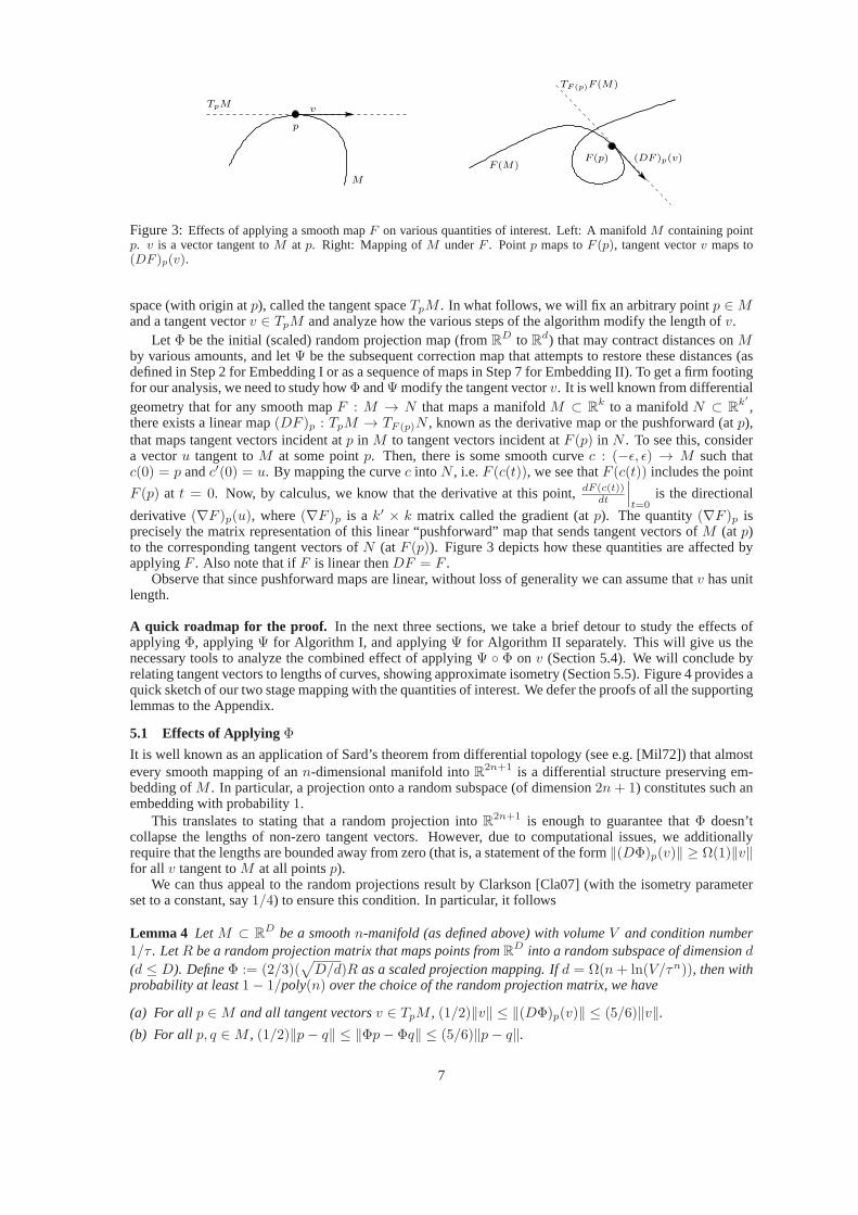
Theorem 3 LetM ⊂ RD be a compactn-manifold with volumeV and condition number1/τ (as above). Let

d = Ω(n+ ln(V/τn)) be the target dimension of the initial random projection mapping such thatd ≤ D.For any 0 < ǫ ≤ 1, let ρ ≤ (τd/D)(ǫ/350)2, δ ≤ (d/D)(ǫ/250)2, and letX ⊂ M be anα-bounded(ρ, δ)-cover ofM . Now, let

i. NI ⊂ Rd+2αn2cn be the embedding ofM returned by AlgorithmI (wherec ≤ 4),

ii. NII ⊂ R2d+3 be the embedding ofM returned by AlgorithmII .

Then, with probability at least1−1/poly(n) over the choice of the initial random projection, for allp, q ∈Mand their corresponding mappingspI, qI ∈ NI andpII, qII ∈ NII, we have

i. (1− ǫ)DG(p, q) ≤ DG(pI, qI) ≤ (1 + ǫ)DG(p, q),

ii. (1− ǫ)DG(p, q) ≤ DG(pII, qII) ≤ (1 + ǫ)DG(p, q).

5 Proof

Our goal is to show that the two proposed embeddings approximately preserve the length of all geodesiccurves. Now, since the length of any given curveγ : [a, b]→M is given by

∫ b

a‖γ′(s)‖ds, it is vital to study

how our embeddings modify the length of the tangent vectors at any pointp ∈M .In order to discuss tangent vectors, we need to introduce thenotion of a tangent spaceTpM at a particular

pointp ∈M . Consider any smooth curvec : (−ǫ, ǫ)→M such thatc(0) = p, then we know thatc′(0) is thevector tangent toc at p. The collection of all such vectors formed by all such curvesis a well defined vector

6

p

v

M

TpM

TF (p)F (M)

F (M)F (p) (DF )p(v)

Figure 3:Effects of applying a smooth mapF on various quantities of interest. Left: A manifoldM containing pointp. v is a vector tangent toM at p. Right: Mapping ofM underF . Pointp maps toF (p), tangent vectorv maps to(DF )p(v).

space (with origin atp), called the tangent spaceTpM . In what follows, we will fix an arbitrary pointp ∈Mand a tangent vectorv ∈ TpM and analyze how the various steps of the algorithm modify thelength ofv.

Let Φ be the initial (scaled) random projection map (fromRD to Rd) that may contract distances onM

by various amounts, and letΨ be the subsequent correction map that attempts to restore these distances (asdefined in Step 2 for Embedding I or as a sequence of maps in Step7 for Embedding II). To get a firm footingfor our analysis, we need to study howΦ andΨ modify the tangent vectorv. It is well known from differentialgeometry that for any smooth mapF : M → N that maps a manifoldM ⊂ R

k to a manifoldN ⊂ Rk′

,there exists a linear map(DF )p : TpM → TF (p)N , known as the derivative map or the pushforward (atp),that maps tangent vectors incident atp in M to tangent vectors incident atF (p) in N . To see this, considera vectoru tangent toM at some pointp. Then, there is some smooth curvec : (−ǫ, ǫ) → M such thatc(0) = p andc′(0) = u. By mapping the curvec intoN , i.e.F (c(t)), we see thatF (c(t)) includes the point

F (p) at t = 0. Now, by calculus, we know that the derivative at this point,dF (c(t))dt

∣∣∣t=0

is the directional

derivative(∇F )p(u), where(∇F )p is a k′ × k matrix called the gradient (atp). The quantity(∇F )p isprecisely the matrix representation of this linear “pushforward” map that sends tangent vectors ofM (at p)to the corresponding tangent vectors ofN (at F (p)). Figure 3 depicts how these quantities are affected byapplyingF . Also note that ifF is linear thenDF = F .

Observe that since pushforward maps are linear, without loss of generality we can assume thatv has unitlength.

A quick roadmap for the proof. In the next three sections, we take a brief detour to study theeffects ofapplyingΦ, applyingΨ for Algorithm I, and applyingΨ for Algorithm II separately. This will give us thenecessary tools to analyze the combined effect of applyingΨ Φ on v (Section 5.4). We will conclude byrelating tangent vectors to lengths of curves, showing approximate isometry (Section 5.5). Figure 4 provides aquick sketch of our two stage mapping with the quantities of interest. We defer the proofs of all the supportinglemmas to the Appendix.

5.1 Effects of ApplyingΦ

It is well known as an application of Sard’s theorem from differential topology (see e.g. [Mil72]) that almostevery smooth mapping of ann-dimensional manifold intoR2n+1 is a differential structure preserving em-bedding ofM . In particular, a projection onto a random subspace (of dimension2n+ 1) constitutes such anembedding with probability1.

This translates to stating that a random projection intoR2n+1 is enough to guarantee thatΦ doesn’t

collapse the lengths of non-zero tangent vectors. However,due to computational issues, we additionallyrequire that the lengths are bounded away from zero (that is,a statement of the form‖(DΦ)p(v)‖ ≥ Ω(1)‖v‖for all v tangent toM at all pointsp).

We can thus appeal to the random projections result by Clarkson [Cla07] (with the isometry parameterset to a constant, say1/4) to ensure this condition. In particular, it follows

Lemma 4 LetM ⊂ RD be a smoothn-manifold (as defined above) with volumeV and condition number

1/τ . LetR be a random projection matrix that maps points fromRD into a random subspace of dimensiond(d ≤ D). DefineΦ := (2/3)(

√

D/d)R as a scaled projection mapping. Ifd = Ω(n+ ln(V/τn)), then withprobability at least1− 1/poly(n) over the choice of the random projection matrix, we have

(a) For all p ∈M and all tangent vectorsv ∈ TpM , (1/2)‖v‖ ≤ ‖(DΦ)p(v)‖ ≤ (5/6)‖v‖.(b) For all p, q ∈M , (1/2)‖p− q‖ ≤ ‖Φp− Φq‖ ≤ (5/6)‖p− q‖.

7

Φ

Rd+k

t = Φp

Ψ

M ΦM

RD

Rd

ΨΦM

p Ψ(t)

v

‖v‖ = 1

u = Φv (DΨ)t(u)

‖(DΨ)t(u)‖ ≈ ‖v‖‖u‖ ≤ 1

Figure 4:Two stage mapping of our embedding technique. Left: Underlying manifold M ⊂ RD with the quantities of

interest – a fixed pointp and a fixed unit-vectorv tangent toM at p. Center: A (scaled) linear projection ofM into arandom subspace ofd dimensions. The pointp maps toΦp and the tangent vectorv maps tou := (DΦ)p(v) = Φv. Thelength ofv contracts to‖u‖. Right: Correction ofΦM via a non-linear mappingΨ into R

d+k. We havek = O(α2cn)for correction technique I, andk = d + 3 for correction technique II (see also Section 4). Our goal is to show thatΨstretches length of contractedv (i.e.u) back to approximately its original length.

(c) For all x ∈ RD, ‖Φx‖ ≤ (2/3)(

√

D/d)‖x‖.

In what follows, we assume thatΦ is such a scaled random projection map. Then, a bound on the length oftangent vectors also gives us a bound on the spectrum ofΦFx (recall the definition ofFx from Section 4).

Corollary 5 LetΦ, Fx andn be as described above (recall thatx ∈ X that forms a bounded(ρ, δ)-coverof M ). Let σi

x represent theith largest singular value of the matrixΦFx. Then, forδ ≤ d/32D, we have1/4 ≤ σn

x ≤ σ1x ≤ 1 (for all x ∈ X).

We will be using these facts in our discussion below in Section 5.4.

5.2 Effects of ApplyingΨ (Algorithm I)

As discussed in Section 2.1, the goal ofΨ is to restore the contraction induced byΦ onM . To understand theaction ofΨ on a tangent vector better, we will first consider a simple case of flat manifolds (Section 5.2.1),and then develop the general case (Section 5.2.2).

5.2.1 Warm-up: flat MLet’s first consider applying a simple one-dimensional spiral mapΨ : R→ R

3 given byt 7→ (t, sin(Ct), cos(Ct)),wheret ∈ I = (−ǫ, ǫ). Let v be a unit vector tangent toI (at, say,0). Then note that

(DΨ)t=0(v) =dΨ

dt

∣∣∣t=0

= (1, C cos(Ct),−C sin(Ct))∣∣t=0

.

Thus, applyingΨ stretches the length ofv from 1 to∥∥(1, C cos(Ct),−C sin(Ct))|t=0

∥∥ =

√1 + C2. No-

tice the advantage of applying the spiral map in computing the lengths: the sine and cosine terms combinetogether to yield a simple expression for the size of the stretch. In particular, if we want to stretch the lengthof v from 1 to, say,L ≥ 1, then we simply needC =

√L2 − 1 (notice the similarity between this expression

and our expression for the diagonal componentSx of the correction matrixCx in Section 4).

We can generalize this to the case ofn-dimensional flat manifold (a section of ann-flat) by considering amap similar toΨ. For concreteness, letF be aD × n matrix whose column vectors form some orthonormalbasis of then-flat manifold (in the original spaceRD). Let UΣV T be the “thin” SVD ofΦF . ThenFVforms an orthonormal basis of then-flat manifold (inR

D) that maps to an orthogonal basisUΣ of theprojectedn-flat manifold (inRd) via the contraction mappingΦ. Define the spiral mapΨ : Rd → R

d+2n

in this case as follows.Ψ(t) := (t, Ψsin(t), Ψcos(t)), with Ψsin(t) := (ψ1sin(t), . . . , ψ

nsin(t)) andΨcos(t) :=

(ψ1cos(t), . . . , ψ

ncos(t)). The individual terms are given as

ψisin(t) := sin((Ct)i)

ψicos(t) := cos((Ct)i)

i = 1, . . . , n,

whereC is now ann× d correction matrix. It turns out that settingC = (Σ−2 − I)1/2UT precisely restoresthe contraction caused byΦ to the tangent vectors (notice the similarity between this expression with the

8

correction matrix in the general caseCx in Section 4 and our motivating intuition in Section 2.1). Tosee this,let v be a vector tangent to then-flat at some pointp (in R

D). We will representv in theFV basis (that is,v =

∑

i αi(Fvi) where[Fv1, . . . , Fvn] = FV ). Note that‖Φv‖2 = ‖∑i αiΦFv

i‖2 = ‖∑i αiσiui‖2 =

∑

i(αiσi)2 (whereσi are the individual singular values ofΣ andui are the left singular vectors forming

the columns ofU ). Now, let w be the pushforward ofv (that is,w = (DΦ)p(v) = Φv =∑

i wiei,

whereeii forms the standard basis ofRd). Now, sinceDΨ is linear, we have‖(DΨ)Φ(p)(w)‖2 =

‖∑i wi(DΨ)Φ(p)(ei)‖2, where(DΨ)Φ(p)(e

i) = dΨdti

∣∣t=Φ(p)

=(

dtdti ,

dΨsin(t)dti , dΨcos(t)

dti

) ∣∣∣t=Φ(p)

. The in-

dividual components are given by

dψksin(t)/dt

i = +cos((Ct)k)Ck,i

dψkcos(t)/dt

i = − sin((Ct)k)Ck,ik = 1, . . . , n; i = 1, . . . , d.

By algebra, we see that

‖(D(Ψ Φ))p(v)‖2 = ‖(DΨ)Φ(p)((DΦ)p(v))‖2 = ‖(DΨ)Φ(p)(w)‖2

=

d∑

k=1

w2k +

n∑

k=1

cos2((CΦ(p))k)((CΦv)k)2 +

n∑

k=1

sin2((CΦ(p))k)((CΦv)k)2

=

d∑

k=1

w2k +

n∑

k=1

((CΦv)k)2 = ‖Φv‖2 + ‖CΦv‖2 = ‖Φv‖2 + (Φv)TCTC(Φv)

= ‖Φv‖2 + (∑

i

αiσiui)TU(Σ−2 − I)UT(

∑

i

αiσiui)

= ‖Φv‖2 + [α1σ1, . . . , αnσ

n](Σ−2 − I)[α1σ1, . . . , αnσ

n]T

= ‖Φv‖2 + (∑

i

α2i −

∑

i

(αiσi)2) = ‖Φv‖2 + ‖v‖2 − ‖Φv‖2 = ‖v‖2.

In other words, our non-linear correction mapΨ canexactlyrestore the contraction caused byΦ for anyvector tangent to ann-flat manifold.

In the fully general case, the situation gets slightly more complicated since we need to apply differentspiral maps, each corresponding to a different size correction at different locations on the contracted manifold.Recall that we localize the effect of a correction by applying the so-called “bump” function (details below).These bump functions, although important for localization, have an undesirable effect on the stretched lengthof the tangent vector. Thus, to ameliorate their effect on the length of the resulting tangent vector, we controltheir contribution via a free parameterω.

5.2.2 The General CaseMore specifically, Embedding Technique I restores the contraction induced byΦ by applying a non-linearmapΨ(t) := (t,Ψ1,sin(t),Ψ1,cos(t), . . . ,ΨK,sin(t),ΨK,cos(t)) (recall thatK is the number of subsets wedecomposeX into – cf. description in Embedding I in Section 4), withΨj,sin(t) := (ψ1

j,sin(t), . . . , ψnj,sin(t))

andΨj,cos(t) := (ψ1j,cos(t), . . . , ψ

nj,cos(t)). The individual terms are given as

ψij,sin(t) :=

∑

x∈X(j) (√

ΛΦ(x)(t)/ω) sin(ω(Cxt)i)

ψij,cos(t) :=

∑

x∈X(j) (√

ΛΦ(x)(t)/ω) cos(ω(Cxt)i)

i = 1, . . . , n; j = 1, . . . ,K,

whereCx’s are the correction amounts for different locationsx on the manifold,ω > 0 controls the frequency(cf. Section 4), andΛΦ(x)(t) is defined to beλΦ(x)(t)/

∑

q∈X λΦ(q)(t), with

λΦ(x)(t) :=

exp(−1/(1− ‖t− Φ(x)‖2/ρ2)) if ‖t− Φ(x)‖ < ρ.0 otherwise.

λ is a classic example of abump function(see Figure 5 middle). It is a smooth function with compactsupport. Its applicability arises from the fact that it can be made “to specifications”. That is, it can bemade to vanish outside any interval of our choice. Here we exploit this property to localize the effect of ourcorrections. The normalization ofλ (the functionΛ) creates the so-called smooth partition of unity that helpsto vary smoothly between the spirals applied at different regions ofM .

Since any tangent vector inRd can be expressed in terms of the basis vectors, it suffices to study howDΨ

acts on the standard basisei. Note that(DΨ)t(ei) =

(dtdti ,

dΨ1,sin(t)dti ,

dΨ1,cos(t)dti , . . . ,

dΨK,sin(t)dti ,

dΨK,cos(t)dti

)∣∣t,

9

−4 −3 −2 −1 0 1 2 3 4

−1

−0.5

0

0.5

1

−1

−0.5

0

0.5

1

−2 −1.5 −1 −0.5 0 0.5 1 1.5 20

0.05

0.1

0.15

0.2

0.25

0.3

0.35

0.4

|t−x|/ρ

λ x(t)

−4 −3 −2 −1 0 1 2 3 4

−0.4

−0.2

0

0.2

0.4

−0.4

−0.3

−0.2

−0.1

0

0.1

0.2

0.3

0.4

Figure 5: Effects of applying a bump function on a spiral mapping. Left: Spiral mapping t 7→ (t, sin(t), cos(t)).Middle: Bump functionλx: a smooth function with compact support. The parameterx controls the location whileρcontrols the width. Right: The combined effect:t 7→ (t, λx(t) sin(t), λx(t) cos(t)). Note that the effect of the spiral islocalized while keeping the mapping smooth.

where

dψkj,sin(t)/dt

i =∑

x∈X(j)1ω

(

sin(ω(Cxt)k)dΛ

1/2

Φ(x)(t)

dti

)

+√ΛΦ(x)(t) cos(ω(C

xt)k)Cxk,i

dψkj,cos(t)/dt

i =∑

x∈X(j)1ω

(

cos(ω(Cxt)k)dΛ

1/2

Φ(x)(t)

dti

)

−√

ΛΦ(x)(t) sin(ω(Cxt)k)C

xk,i

k = 1, . . . , n; i = 1, . . . , dj = 1, . . . ,K

.

One can now observe the advantage of having the termω. By pickingω sufficiently large, we can make thefirst part of the expression sufficiently small. Now, for any tangent vectoru =

∑

i uiei such that‖u‖ ≤ 1,

we have (by algebra)

‖(DΨ)t(u)‖2 =∥∥∥

∑

ui(DΨ)t(ei)∥∥∥

2

=d∑

k=1

u2k +n∑

k=1

K∑

j=1

[ ∑

x∈X(j)

(Ak,xsin (t)

ω

)

+√

ΛΦ(x)(t) cos(ω(Cxt)k)(C

xu)k

]2

+[ ∑

x∈X(j)

(Ak,xcos(t)

ω

)

−√

ΛΦ(x)(t) sin(ω(Cxt)k)(C

xu)k

]2

(1)

whereAk,xsin (t) :=

∑

i ui sin(ω(Cxt)k)(dΛ

1/2Φ(x)(t)/dt

i) andAk,xcos(t) :=

∑

i ui cos(ω(Cxt)k)(dΛ

1/2Φ(x)(t)/dt

i).We can further simplify Eq. (1) and get

Lemma 6 Let t be any point inΦ(M) andu be any vector tagent toΦ(M) at t such that‖u‖ ≤ 1. Letǫ bethe isometry parameter chosen in Theorem 3. Pickω ≥ Ω(nα29n

√d/ρǫ), then

‖(DΨ)t(u)‖2 = ‖u‖2 +∑

x∈X

ΛΦ(x)(t)

n∑

k=1

(Cxu)2k + ζ, (2)

where|ζ| ≤ ǫ/2.

We will use this derivation of‖(DΨ)t(u)‖2 to study the combined effect ofΨ Φ onM in Section 5.4.

5.3 Effects of ApplyingΨ (Algorithm II)

The goal of the second algorithm is to apply the spiralling corrections while using the coordinates moreeconomically. We achieve this goal by applying them sequentially in the same embedding space (rather thansimultaneously by making use of extra2nK coordinates as done in the first algorithm), see also [Nas54].Since all the corrections will be sharing the same coordinate space, one needs to keep track of a pair ofnormal vectors in order to prevent interference among the different local corrections.

More specifically,Ψ : Rd → R2d+3 (in Algorithm II) is defined recursively asΨ := Ψ|X|,n such that

(see also Embedding II in Section 4)

Ψi,j(t) := Ψi,j−1(t) + ηi,j(t)

√ΛΦ(xi)(t)

ωi,jsin(ωi,j(C

xit)j) + νi,j(t)

√ΛΦ(xi)(t)

ωi,jcos(ωi,j(C

xit)j),

whereΨi,0(t) := Ψi−1,n(t), and the base functionΨ0,n(t) is given ast 7→ (t,

d+3︷ ︸︸ ︷

0, . . . , 0). ηi,j(t) andνi,j(t)are mutually orthogonal unit vectors that are approximately normal toΨi,j−1(ΦM) at Ψi,j−1(t). In thissection we assume that the normalsη andν have the following properties:

10

- |ηi,j(t) · v| ≤ ǫ0 and|νi,j(t) · v| ≤ ǫ0 for all unit-lengthv tangent toΨi,j−1(ΦM) atΨi,j−1(t). (quality ofnormal approximation)

- For all 1 ≤ l ≤ d, we have‖dηi,j(t)/dtl‖ ≤ Ki,j and‖dνi,j(t)/dtl‖ ≤ Ki,j . (bounded directionalderivatives)

We refer the reader to Section A.9 for details on how to estimate such normals.

Now, as before, representing a tangent vectoru =∑

l ulel (such that‖u‖2 ≤ 1) in terms of its basis

vectors, it suffices to study howDΨ acts on basis vectors. Observe that(DΨi,j)t(el) =

(dΨi,j(t)

dtl

)2d+3

k=1

∣∣∣t,

with thekth component given as(dΨi,j−1(t)

dtl

)

k

+ (ηi,j(t))k

√

ΛΦ(xi)(t)Cxi

j,lBi,jcos(t)− (νi,j(t))k

√

ΛΦ(xi)(t)Cxi

j,lBi,jsin(t)

+1

ωi,j

[(dηi,j(t)

dtl

)

k

√

ΛΦ(xi)(t)Bi,jsin(t) +

(dνi,j(t)

dtl

)

k

√

ΛΦ(xi)(t)Bi,jcos(t)

+ (ηi,j(t))kdΛ

1/2Φ(xi)

(t)

dtlBi,j

sin(t) + (νi,j(t))kdΛ

1/2Φ(xi)

(t)

dtlBi,j

cos(t)]

,

whereBi,jcos(t) := cos(ωi,j(C

xit)j) andBi,jsin(t) := sin(ωi,j(C

xit)j). For ease of notation, letRk,li,j be the

terms in the bracket (being multiplied to1/ωi,j) in the above expression. Then, we have (for anyi, j)

‖(DΨi,j)t(u)‖2 =∥∥∑

l

ul(DΨi,j)t(el)∥∥2

=

2d+3∑

k=1

[∑

l

ul

(dΨi,j−1(t)

dtl

)

k︸ ︷︷ ︸

ζk,1i,j

+(ηi,j(t))k

√

ΛΦ(xi)(t) cos(ωi,j(Cxit)j)

∑

l

Cxi

j,lul

︸ ︷︷ ︸

ζk,2i,j

−(νi,j(t))k√

ΛΦ(xi)(t) sin(ωi,j(Cxit)j)

∑

l

Cxi

j,lul

︸ ︷︷ ︸

ζk,3i,j

+(1/ωi,j)∑

l

ulRk,li,j

︸ ︷︷ ︸

ζk,4i,j

]2

= ‖(DΨi,j−1)t(u)‖2︸ ︷︷ ︸

=∑

k

(ζk,1i,j

)2

+ ΛΦ(xi)(t)(Cxiu)2j

︸ ︷︷ ︸

=∑

k

(ζk,2i,j

)2+(ζk,3i,j

)2

+∑

k

[(ζk,4i,j /ωi,j

)2+(2ζk,4i,j /ωi,j

)(ζk,1i,j + ζk,2i,j + ζk,3i,j

)+ 2(ζk,1i,j ζ

k,2i,j + ζk,1i,j ζ

k,3i,j

)]

︸ ︷︷ ︸

Zi,j

, (3)

where the last equality is by expanding the square and by noting that∑

k ζk,2i,j ζ

k,3i,j = 0 sinceη andν are

orthogonal to each other. The base case‖(DΨ0,n)t(u)‖2 equals‖u‖2.

Again, by pickingωi,j sufficiently large, and by noting that the cross terms∑

k(ζk,1i,j ζ

k,2i,j ) and

∑

k(ζk,1i,j ζ

k,3i,j )

are very close to zero sinceη andν are approximately normal to the tangent vector, we have

Lemma 7 Let t be any point inΦ(M) andu be any vector tagent toΦ(M) at t such that‖u‖ ≤ 1. Letǫ bethe isometry parameter chosen in Theorem 3. Pickωi,j ≥ Ω

((Ki,j +(α9n/ρ))(nd|X|)2/ǫ

)(recall thatKi,j

is the bound on the directional derivate ofη andν). If ǫ0 ≤ O(ǫ/d(n|X|)2

)(recall thatǫ0 is the quality of

approximation of the normalsη andν), then we have

‖(DΨ)t(u)‖2 = ‖(DΨ|X|,n)t(u)‖2 = ‖u‖2 +|X|∑

i=1

ΛΦ(xi)(t)n∑

j=1

(Cxiu)2j + ζ, (4)

where|ζ| ≤ ǫ/2.

11

5.4 Combined Effect ofΨ(Φ(M))

We can now analyze the aggregate effect of both our embeddings on the length of an arbitrary unit vectorvtangent toM at p. Let u := (DΦ)p(v) = Φv be the pushforward ofv. Then‖u‖ ≤ 1 (cf. Lemma 4). Seealso Figure 4.

Now, recalling thatD(Ψ Φ) = DΨ DΦ, and noting that pushforward maps are linear, we have

‖(D(Ψ Φ))p(v)‖2 =∥∥(DΨ)Φ(p)(u)

∥∥2. Thus, representingu as

∑

i uiei in ambient coordinates ofRd, and

using Eq. (2) (for Algorithm I) or Eq. (4) (for Algorithm II),we get

∥∥(D(Ψ Φ))p(v)

∥∥2

=∥∥(DΨ)Φ(p)(u)

∥∥2= ‖u‖2 +

∑

x∈X

ΛΦ(x)(Φ(p))‖Cxu‖2 + ζ,

where |ζ| ≤ ǫ/2. We can give simple lower and upper bounds for the above expression by noting thatΛΦ(x) is a localization function. DefineNp := x ∈ X : ‖Φ(x) − Φ(p)‖ < ρ as the neighborhoodaroundp (ρ as per the theorem statement). Then only the points inNp contribute to above equation, sinceΛΦ(x)(Φ(p)) = dΛΦ(x)(Φ(p))/dt

i = 0 for ‖Φ(x)−Φ(p)‖ ≥ ρ. Also note that for allx ∈ Np, ‖x−p‖ < 2ρ(cf. Lemma 4).

Let xM := argmaxx∈Np‖Cxu‖2 andxm := argminx∈Np

‖Cxu‖2 are quantities that attain the maxi-mum and the minimum respectively, then:

‖u‖2 + ‖Cxmu‖2 − ǫ/2 ≤ ‖(D(Ψ Φ))p(v)‖2 ≤ ‖u‖2 + ‖CxMu‖2 + ǫ/2. (5)

Notice that ideally we would like to have the correction factor “Cpu” in Eq. (5) since that would give theperfect stretch around the pointp. But what about correctionCxu for closebyx’s? The following lemmahelps us continue in this situation.

Lemma 8 Let p, v, u be as above. For anyx ∈ Np ⊂ X, letCx andFx also be as discussed above (recallthat ‖p − x‖ < 2ρ, andX ⊂ M forms a bounded(ρ, δ)-cover of the fixed underlying manifoldM withcondition number1/τ ). Defineξ := (4ρ/τ) + δ + 4

√

ρδ/τ . If ρ ≤ τ/4 andδ ≤ d/32D, then

1− ‖u‖2 − 40 ·max√

ξD/d, ξD/d≤ ‖Cxu‖2 ≤ 1− ‖u‖2 + 51 ·max

√

ξD/d, ξD/d.

Note that we choseρ ≤ (τd/D)(ǫ/350)2 and δ ≤ (d/D)(ǫ/250)2 (cf. theorem statement). Thus,combining Eq. (5) and Lemma 8, we get (recall‖v‖ = 1)

(1− ǫ)‖v‖2 ≤ ‖(D(Ψ Φ))p(v)‖2 ≤ (1 + ǫ)‖v‖2.

So far we have shown that our embedding approximately preserves the length of a fixed tangent vectorat a fixed point. Since the choice of the vector and the point was arbitrary, it follows that our embeddingapproximately preserves the tangent vector lengths throughout the embedded manifold uniformly. We willnow show that preserving the tangent vector lengths impliespreserving the geodesic curve lengths.

5.5 Preservation of the Geodesics

Pick any two (path-connected) pointsp andq in M , and letα be the geodesic5 path betweenp andq. Furtherlet p, q andα be the images ofp, q andα under our embedding. Note thatα is not necessarily the geodesicpath betweenp and q, thus we need an extra piece of notation: letβ be the geodesic path betweenp and q(under the embedded manifold) andβ be its inverse image inM . We need to show(1 − ǫ)L(α) ≤ L(β) ≤(1 + ǫ)L(α), whereL(·) denotes the length of the path· (end points are understood).

First recall that for any differentiable mapF and curveγ, γ = F (γ) ⇒ γ′ = (DF )(γ′). By (1 ± ǫ)-isometry of tangent vectors, this immediately gives us(1− ǫ)L(γ) ≤ L(γ) ≤ (1 + ǫ)L(γ) for any pathγ inM and its imageγ in embedding ofM . So,

(1− ǫ)DG(p, q) = (1− ǫ)L(α) ≤ (1− ǫ)L(β) ≤ L(β) = DG(p, q).

Similarly,

DG(p, q) = L(β) ≤ L(α) ≤ (1 + ǫ)L(α) = (1 + ǫ)DG(p, q).

5Globally, geodesic paths between points are not necessarily unique; we are interested in a path that yields the shortestdistance between the points.

12

6 Conclusion

This work provides two simple algorithms for approximate isometric embedding of manifolds. Our algo-rithms are similar in spirit to Nash’sC1 construction [Nas54], and manage to remove the dependence on theisometry constantǫ from the target dimension. One should observe that this dependency does however showup in the sampling density required to make the necessary corrections.

The correction procedure discussed here can also be readilyadapted to create isometric embeddings fromany manifold embedding procedure (under some mild conditions). Take any off-the-shelf manifold embed-ding algorithmA (such as LLE, Laplacian Eigenmaps, etc.) that maps ann-manifold in, say,d dimensions,but does not necessarily guarantee an approximate isometric embedding. Then as long as one can ensure thatthe embedding produced byA is a one-to-one contraction6 (basically ensuring conditions similar to Lemma4), we can apply corrections similar to those discussed in Algorithms I or II to produce an approximate iso-metric embedding of the given manifold in slightly higher dimensions. In this sense, the correction procedurepresented here serves as auniversal procedurefor approximate isometric manifold embeddings.

Acknowledgements

The author would like to thank Sanjoy Dasgupta for introducing the subject, and for his guidance throughoutthe project.

References

[BN03] M. Belkin and P. Niyogi. Laplacian eigenmaps for dimensionality reduction and data represen-tation. Neural Computation, 15(6):1373–1396, 2003.

[BW07] R. Baraniuk and M. Wakin. Random projections of smoothmanifolds.Foundations of Compu-tational Mathematics, 2007.

[Cla07] K. Clarkson. Tighter bounds for random projectionsof manifolds.Comp. Geometry, 2007.[DF08] S. Dasgupta and Y. Freund. Random projection trees and low dimensional manifolds.ACM

Symposium on Theory of Computing, 2008.[DG03] D. Donoho and C. Grimes. Hessian eigenmaps: locally linear embedding techniques for high

dimensional data.Proc. of National Academy of Sciences, 100(10):5591–5596, 2003.[DGGZ02] T. Dey, J. Giesen, S. Goswami, and W. Zhao. Shape dimension and approximation from samples.

Symposium on Discrete Algorithms, 2002.[GW03] J. Giesen and U. Wagner. Shape dimension and intrinsicmetric from samples of manifolds with

high co-dimension.Symposium on Computational Geometry, 2003.[HH06] Q. Han and J. Hong.Isometric embedding of Riemannian manifolds in Euclidean spaces. Amer-

ican Mathematical Society, 2006.[JL84] W. Johnson and J. Lindenstrauss. Extensions of Lipschitz mappings into a Hilbert space.Conf.

in Modern Analysis and Probability, pages 189–206, 1984.[Kui55] N. Kuiper. OnC1-isometric embeddings, I, II.Indag. Math., 17:545–556, 683–689, 1955.[Mil72] J. Milnor. Topology from the differential viewpoint. Univ. of Virginia Press, 1972.[Nas54] J. Nash.C1 isometric imbeddings.Annals of Mathematics, 60(3):383–396, 1954.[Nas56] J. Nash. The imbedding problem for Riemannian manifolds. Annals of Mathematics, 63(1):20–

63, 1956.[NSW06] P. Niyogi, S. Smale, and S. Weinberger. Finding the homology of submanifolds with high confi-

dence from random samples.Disc. Computational Geometry, 2006.[RS00] S. Roweis and L. Saul. Nonlinear dimensionality reduction by locally linear embedding.Science,

290, 2000.[TdSL00] J. Tenebaum, V. de Silva, and J. Langford. A global geometric framework for nonlinear dimen-

sionality reduction.Science, 290, 2000.[Whi36] H. Whitney. Differentiable manifolds.Annals of Mathematics, 37:645–680, 1936.[WS04] K. Weinberger and L. Saul. Unsupervised learning of image manifolds by semidefinite program-

ming. Computer Vision and Pattern Recognition, 2004.

6One can modifyA to produce a contraction by simple scaling.

13

A Appendix

A.1 Properties of a Well-conditioned Manifold

Throughout this section we will assume thatM is a compact submanifold ofRD of dimensionn, and condi-tion number1/τ . The following are some properties of such a manifold that would be useful throughout thetext.

Lemma 9 (relating closeby tangent vectors – implicit in the proof of Proposition 6.2 [NSW06]) Pickany two (path-connected) pointsp, q ∈ M . Let u ∈ TpM be a unit length tangent vector andv ∈ TqMbe its parallel transport along the (shortest) geodesic path to q. Then7, i) u · v ≥ 1 − DG(p, q)/τ , ii)‖u− v‖ ≤

√

2DG(p, q)/τ .

Lemma 10 (relating geodesic distances to ambient distances– Proposition 6.3 of [NSW06])If p, q ∈Msuch that‖p− q‖ ≤ τ/2, thenDG(p, q) ≤ τ(1−

√

1− 2‖p− q‖/τ) ≤ 2‖p− q‖.

Lemma 11 (projection of a section of a manifold onto the tangent space)Pick anyp ∈ M and defineMp,r := q ∈ M : ‖q − p‖ ≤ r. Let f denote the orthogonal linear projection ofMp,r onto the tangentspaceTpM . Then, for anyr ≤ τ/2

(i) the mapf :Mp,r → TpM is 1− 1. (see Lemma 5.4 of [NSW06])

(ii) for any x, y ∈ Mp,r, ‖f(x) − f(y)‖2 ≥ (1 − (r/τ)2) · ‖x − y‖2. (implicit in the proof of Lemma 5.3of [NSW06])

Lemma 12 (coverings of a section of a manifold)Pick anyp ∈M and defineMp,r := q ∈M : ‖q−p‖ ≤r. If r ≤ τ/2, then there existsC ⊂ Mp,r of size at most9n with the property: for anyp′ ∈ Mp,r, existsc ∈ C such that‖p′ − c‖ ≤ r/2.

Proof: The proof closely follows the arguments presented in the proof of Theorem 22 of [DF08].For r ≤ τ/2, note thatMp,r ⊂ R

D is (path-)connected. Letf denote the projection ofMp,r ontoTpM ∼= R

n. Quickly note thatf is 1 − 1 (see Lemma 11(i)). Then,f(Mp,r) ⊂ Rn is contained in an

n-dimensional ball of radiusr. By standard volume arguments,f(Mp,r) can be covered by at most9n ballsof radiusr/4. WLOG we can assume that the centers of these covering balls are in f(Mp,r). Now, notingthat the inverse image of each of these covering balls (inR

n) is contained in aD-dimensional ball of radiusr/2 (see Lemma 11(ii)) finishes the proof.

Lemma 13 (relating closeby manifold points to tangent vectors) Pick any pointp ∈ M and letq ∈ M(distinct fromp) be such thatDG(p, q) ≤ τ . Letv ∈ TpM be the projection of the vectorq − p ontoTpM .

Then, i)∣∣∣

v‖v‖ ·

q−p‖q−p‖

∣∣∣ ≥ 1− (DG(p, q)/2τ)

2, ii)∥∥∥

v‖v‖ −

q−p‖q−p‖

∥∥∥ ≤ DG(p, q)/τ

√2.

Proof: If vectorsv andq − p are in the same direction, we are done. Otherwise, consider the plane spannedby vectorsv andq − p. Then sinceM has condition number1/τ , we know that the pointq cannot lie withinanyτ -ball tangent toM atp (see Figure 6). Consider such aτ -ball (with centerc) whose center is closest toq and letq′ be the point on the surface of the ball which subtends the sameangle (∠pcq′) as the angle formedby q (∠pcq). Let this angle be calledθ. Then using cosine rule, we havecos θ = 1− ‖q′ − p‖2/2τ2.

Defineα as the angle subtended by vectorsv andq − p, andα′ the angle subtended by vectorsv andq′ − p. WLOG we can assume that the anglesα andα′ are less thanπ. Then,cosα ≥ cosα′ = cos θ/2.Using the trig identitycos θ = 2 cos2

(θ2

)− 1, and noting‖q − p‖2 ≥ ‖q′ − p‖2, we have

∣∣∣∣

v

‖v‖ ·q − p‖q − p‖

∣∣∣∣= cosα ≥ cos

θ

2≥√

1− ‖q − p‖2/4τ2 ≥ 1− (DG(p, q)/2τ)2.

Now, by applying the cosine rule, we have∥∥ v‖v‖ −

q−p‖q−p‖

∥∥2= 2(1− cosα). The lemma follows.

7Technically, it is not possible to directly compare two vectors that reside in different tangent spaces. However, sincewe only deal with manifolds that are immersed in some ambient space, we can treat the tangent spaces asn-dimensionalaffine subspaces. We can thus parallel translate the vectors to the origin of the ambient space, and do the necessarycomparison (such as take the dot product, etc.). We will make a similar abuse of notation for any calculation that usesvectors from different affine subspaces to mean to first translate the vectors and then perform the necessary calculation.

14

q

TpM

q′θ

τ

p

c

v

Figure 6:Plane spanned by vectorsq − p andv ∈ TpM (wherev is the projection ofq − p ontoTpM ), with τ -ballstangent top. Note thatq′ is the point on the ball such that∠pcq = ∠pcq′ = θ.

Lemma 14 (approximating tangent space by closeby samples)Let 0 < δ ≤ 1. Pick any pointp0 ∈ Mand letp1, . . . , pn ∈M ben points distinct fromp0 such that (for all1 ≤ i ≤ n)

(i) DG(p0, pi) ≤ τδ/√n,

(ii)∣∣ pi−p0

‖pi−p0‖· pj−p0

‖pj−p0‖

∣∣ ≤ 1/2n (for i 6= j).

Let T be then dimensional subspace spanned by vectorspi − p0i∈[n]. For any unit vectoru ∈ T , letu bethe projection ofu ontoTp0

M . Then,∣∣u · u

‖u‖

∣∣ ≥ 1− δ.

Proof: Define the vectorsvi := pi−p0

‖pi−p0‖(for 1 ≤ i ≤ n). Observe thatvii∈[n] forms a basis ofT . For

1 ≤ i ≤ n, definevi as the projection of vectorvi ontoTp0M . Also note that by applying Lemma 13, we

have that for all1 ≤ i ≤ n, ‖vi − vi‖2 ≤ δ2/2n.Let V = [v1, . . . , vn] be theD× n matrix. We represent the unit vectoru asV α =

∑

i αivi. Also, sinceu is the projection ofu, we haveu =

∑

i αivi. Then,‖α‖2 ≤ 2. To see this, we first identifyT with Rn

via an isometryS (a linear map that preserves the lengths and angles of all vectors inT ). Note thatS can berepresented as ann × D matrix, and sinceV forms a basis forT , SV is ann × n invertible matrix. Then,sinceSu = SV α, we haveα = (SV )

−1Su. Thus, (recall‖Su‖ = 1)

‖α‖2 ≤ maxx∈Sn−1

‖(SV )−1x‖2 = λmax((SV )−T(SV )−1)

= λmax((SV )−1(SV )−T) = λmax((VTV )−1) = 1/λmin(V

TV )

≤ 1/1− ((n− 1)/2n) ≤ 2,

where i)λmax(A) andλmin(A) denote the largest and smallest eigenvalues of a square symmetric matrixArespectively, and ii) the second inequality is by noting that V TV is ann× n matrix with1’s on the diagonaland at most1/2n on the off-diagonal elements, and applying the Gershgorin circle theorem.

Now we can bound the quantity of interest. Note that∣∣∣u · u

‖u‖∣∣∣ ≥ |uT(u− (u− u))| ≥ 1− ‖u− u‖ = 1−

∥∥∑

i

αi(vi − vi)∥∥

≥ 1−∑

i

|αi|‖vi − vi‖ ≥ 1− (δ/√2n)

∑

i

|αi| ≥ 1− δ,

where the last inequality is by noting‖α‖1 ≤√2n.

A.2 On Constructing a Bounded Manifold Cover

Given a compactn-manifoldM ⊂ RD with condition number1/τ , and some0 < δ ≤ 1. We can construct

anα-bounded(ρ, δ) coverX of M (with α ≤ 210n+1 andρ ≤ τδ/3√2n) as follows.

Setρ ≤ τδ/3√2n and pick a(ρ/2)-netC of M (that isC ⊂ M such that, i. forc, c′ ∈ C such that

c 6= c′, ‖c−c′‖ ≥ ρ/2, ii. for all p ∈M , existsc ∈ C such that‖c−p‖ < ρ/2). WLOG we shall assume thatall points ofC are in the interior ofM . Then, for eachc ∈ C, defineMc,ρ/2 := p ∈ M : ‖p− c‖ ≤ ρ/2,and the orthogonal projection mapfc :Mc,ρ/2 → TcM that projectsMc,ρ/2 ontoTcM (note that, cf. Lemma

15

11(i),fc is 1−1). Note thatTcM can be identified withRn with thec as the origin. We will denote the originasx(c)0 , that is,x(c)0 = fc(c).

Now, letBc be anyn-dimensional closed ball centered at the originx(c)0 ∈ TcM of radiusr > 0 that is

completely contained infc(Mc,ρ/2) (that is,Bc ⊂ fc(Mc,ρ/2)). Pick a set ofn pointsx(c)1 , . . . , x(c)n on the

surface of the ballBc such that(x(c)i − x(c)0 ) · (x(c)j − x

(c)0 ) = 0 for i 6= j.

Define the bounded manifold cover as

X :=⋃

c∈C,i=0,...,n

f−1c (x

(c)i ). (6)

Lemma 15 Let0 < δ ≤ 1 andρ ≤ τδ/3√2n. LetC be a(ρ/2)-net ofM as described above, andX be as

in Eq. (6). ThenX forms a210n+1-bounded(ρ, δ) cover ofM .

Proof: Pick any pointp ∈ M and defineXp := x ∈ X : ‖x − p‖ < ρ. Let c ∈ C be such that‖p− c‖ < ρ/2. ThenXp has the following properties.

Covering criterion:For 0 ≤ i ≤ n, since‖f−1c (x

(c)i ) − c‖ ≤ ρ/2 (by construction), we have‖f−1

c (x(c)i ) −

p‖ < ρ. Thus,f−1c (x

(c)i ) ∈ Xp (for 0 ≤ i ≤ n). Now, for1 ≤ i ≤ n, noting thatDG(f

−1c (x

(c)i ), f−1

c (x(c)0 )) ≤

2‖f−1c (x

(c)i )−f−1

c (x(c)0 )‖ ≤ ρ (cf. Lemma 10), we have that for the vectorv(c)i :=

f−1c (x

(c)i )−f−1

c (x(c)0 )

‖f−1c (x

(c)i )−f−1

c (x(c)0 )‖

and

its (normalized) projectionv(c)i :=x(c)i −x

(c)0

‖x(c)i −x

(c)0 ‖

ontoTcM ,∥∥v

(c)i − v

(c)i

∥∥ ≤ ρ/

√2τ (cf. Lemma 13). Thus,

for i 6= j, we have (recall, by construction, we havev(c)i · v(c)j = 0)

|v(c)i · v(c)j | = |(v(c)i − v

(c)i + v

(c)i ) · (v(c)j − v

(c)j + v

(c)j )|

= |(v(c)i − v(c)i ) · (v(c)j − v

(c)j ) + v

(c)i · (v

(c)j − v

(c)j ) + (v

(c)i − v

(c)i ) · v(c)j |

≤ ‖(v(c)i − v(c)i )‖‖(v(c)j − v

(c)j )‖+ ‖v(c)i − v

(c)i ‖+ ‖v

(c)j − v

(c)j ‖

≤ 3ρ/√2τ ≤ 1/2n.

Point representation criterion:There existsx ∈ Xp, namelyf−1c (x

(c)0 ) (= c), such that‖p− x‖ ≤ ρ/2.

Local boundedness criterion:DefineMp,3ρ/2 := q ∈M : ‖q − p‖ < 3ρ/2. Note thatXp ⊂ f−1c (x

(c)i ) :

c ∈ C ∩Mp,3ρ/2, 0 ≤ i ≤ n. Now, using Lemma 12 we have that exists a coverN ⊂ Mp,3ρ/2 of sizeat most93n such that for any pointq ∈ Mp,3ρ/2, there existsn ∈ N such that‖q − n‖ < ρ/4. Note that,by construction ofC, there cannot be ann ∈ N such that it is within distanceρ/4 of two (or more) distinctc, c′ ∈ C (since otherwise the distance‖c− c′‖ will be less thanρ/2, contradicting the packing ofC). Thus,|C ∩Mp,3ρ/2| ≤ 93n. It follows that|Xp| ≤ (n+ 1)93n ≤ 210n+1.

Tangent space approximation criterion:Let Tp be then-dimensional span ofv(c)i i∈[n] (note thatTp may

not necessarily pass throughp). Then, for any unit vectoru ∈ Tp, we need to show that its projectionupontoTpM has the property|u · up

‖up‖| ≥ 1 − δ. Let θ be the angle between vectorsu andup. Let uc be the

projection ofu ontoTcM , andθ1 be the angle between vectorsu anduc, and letθ2 be the angle betweenvectorsuc (at c) and its parallel transport along the geodesic path top. WLOG we can assume thatθ1 andθ2are at mostπ/2. Then,θ ≤ θ1 + θ2 ≤ π. We get the bound on the individual angles as follows. By applyingLemma 14,cos(θ1) ≥ 1− δ/4, and by applying Lemma 9,cos(θ2) ≥ 1− δ/4. Finally, by using Lemma 16,we have

∣∣u · up

‖up‖

∣∣ = cos(θ) ≥ cos(θ1 + θ2) ≥ 1− δ.

Lemma 16 Let0 ≤ ǫ1, ǫ2 ≤ 1. If cosα ≥ 1−ǫ1 andcosβ ≥ 1−ǫ2, thencos(α+β) ≥ 1−ǫ1−ǫ2−2√ǫ1ǫ2.

Proof: Applying the identitysin θ =√1− cos2 θ immediately yieldssinα ≤

√2ǫ1 andsinβ ≤

√2ǫ2.

Now, cos(α+ β) = cosα cosβ − sinα sinβ ≥ (1− ǫ1)(1− ǫ2)− 2√ǫ1ǫ2 ≥ 1− ǫ1 − ǫ2 − 2

√ǫ1ǫ2.

Remark 6 A dense enough sample fromM constitutes as a bounded cover. One can selectively prune thedense sampling to control the total number of points in each neighborhood, while still maintaining the coverproperties.

16

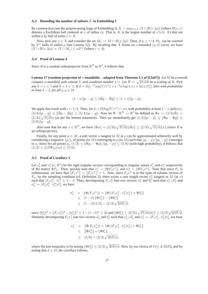
A.3 Bounding the number of subsetsK in Embedding I

By construction (see the preprocessing stage of Embedding I),K = maxx∈X |X ∩B(x, 2ρ)| (whereB(x, r)denotes a Euclidean ball centered atx of radiusr). That is,K is the largest number ofx’s (∈ X) that arewithin a2ρ ball of somex ∈ X.

Now, pick anyx ∈ X and consider the setMx := M ∩ B(x, 2ρ). Then, ifρ ≤ τ/4, Mx can be coveredby 2cn balls of radiusρ (see Lemma 12). By recalling thatX forms anα-bounded(ρ, δ)-cover, we have|X ∩B(x, 2ρ)| = |X ∩Mx| ≤ α2cn (wherec ≤ 4).

A.4 Proof of Lemma 4

SinceR is a random orthoprojector fromRD toRd, it follows that

Lemma 17 (random projection ofn-manifolds – adapted from Theorem 1.5 of [Cla07])LetM be a smoothcompactn-manifold with volumeV and condition number1/τ . Let R :=

√

D/dR be a scaling ofR. Pickany0 < ǫ ≤ 1 and0 < δ ≤ 1. If d = Ω

(ǫ−2 log(V/τn) + ǫ−2n log(1/ǫ) + ln(1/δ)

), then with probability

at least1− δ, for all p, q ∈M

(1− ǫ)‖p− q‖ ≤ ‖Rp− Rq‖ ≤ (1 + ǫ)‖p− q‖.

We apply this result withǫ = 1/4. Then, ford = Ω(log(V/τn)+n), with probability at least1− 1/poly(n),(3/4)‖p − q‖ ≤ ‖Rp − Rq‖ ≤ (5/4)‖p − q‖. Now letΦ : RD → R

d be defined asΦx := (2/3)Rx =

(2/3)(√

D/d)x (as per the lemma statement). Then we immediately get(1/2)‖p − q‖ ≤ ‖Φp − Φq‖ ≤(5/6)‖p− q‖.

Also note that for anyx ∈ RD, we have‖Φx‖ = (2/3)(

√

D/d)‖Rx‖ ≤ (2/3)(√

D/d)‖x‖ (sinceR isan orthoprojector).

Finally, for any pointp ∈ M , a unit vectoru tangent toM at p can be approximated arbitrarily well byconsidering a sequencepii of points (inM ) converging top (in M ) such that(pi− p)/‖pi − p‖ convergesto u. Since for all pointspi, (1/2) ≤ ‖Φpi − Φp‖/‖pi − p‖ ≤ (5/6) (with high probability), it follows that(1/2) ≤ ‖(DΦ)p(u)‖ ≤ (5/6).

A.5 Proof of Corollary 5

Let v1x andvnx (∈ Rn) be the right singular vectors corresponding to singular valuesσ1

x andσnx respectively

of the matrixΦFx. Then, quickly note thatσ1x = ‖ΦFxv

1‖, andσnx = ‖ΦFxv

n‖. Note that sinceFx isorthonormal, we have that‖Fxv

1‖ = ‖Fxvn‖ = 1. Now, sinceFxv

n is in the span of column vectors ofFx, by the sampling condition (cf. Definition 2), there exists aunit length vectorvnx tangent toM (at x)such that|Fxv

nx · vnx | ≥ 1 − δ. Thus, decomposingFxv

nx into two vectorsanx andbnx such thatanx⊥bnx and

anx := (Fxvnx · vnx )vnx , we have

σnx = ‖Φ(Fxv

n)‖ = ‖Φ((Fxvnx · vnx )vnx ) + Φbnx‖

≥ (1− δ) ‖Φvnx‖ − ‖Φbnx‖≥ (1− δ)(1/2)− (2/3)

√

2δD/d,

since‖bnx‖2 = ‖Fxvnx‖2−‖anx‖2 ≤ 1− (1− δ)2 ≤ 2δ and‖Φbnx‖ ≤ (2/3)(

√

D/d)‖bnx‖ ≤ (2/3)√

2δD/d.Similarly decomposingFxv

1x into two vectorsa1x andb1x such thata1x⊥b1x anda1x := (Fxv

1x · v1x)v1x, we have

σ1x = ‖Φ(Fxv

1x)‖ = ‖Φ((Fxv

1x · v1x)v1x) + Φb1x‖

≤∥∥Φv1x

∥∥+ ‖Φb1x‖

≤ (5/6) + (2/3)√

2δD/d,

where the last inequality is by noting‖Φb1x‖ ≤ (2/3)√

2δD/d. Now, by our choice ofδ (≤ d/32D), and bynoting thatd ≤ D, the corollary follows.

17

A.6 Proof of Lemma 6

We can simplify Eq. (1) by recalling how the subsetsX(j) were constructed (see preprocessing stage ofEmbedding I). Note that for any fixedt, at most one term in the setΛΦ(x)(t)x∈X(j) is non-zero. Thus,

‖(DΨ)t(u)‖2 =

d∑

k=1

u2k +

n∑

k=1

∑

x∈X

ΛΦ(x)(t) cos2(ω(Cxt)k)(C

xu)2k + ΛΦ(x)(t) sin2(ω(Cxt)k)(C

xu)2k

+1

ω

[ ((Ak,x

sin (t))2

+(Ak,x

cos(t))2)

/ω︸ ︷︷ ︸

ζ1

+2Ak,xsin (t)

√

ΛΦ(x)(t) cos(ω(Cxt)k)(C

xu)k︸ ︷︷ ︸

ζ2

−2Ak,xcos(t)

√

ΛΦ(x)(t) sin(ω(Cxt)k)(C

xu)k︸ ︷︷ ︸

ζ3

]

= ‖u‖2 +∑

x∈X

ΛΦ(x)(t)n∑

k=1

(Cxu)2k + ζ,

whereζ := (ζ1 + ζ2 + ζ3)/ω. Noting that i) the terms|Ak,xsin (t)| and |Ak,x

cos(t)| are at mostO(α9n√d/ρ)

(see Lemma 18), ii)|(Cxu)k| ≤ 4, and iii)√ΛΦ(x)(t) ≤ 1, we can pickω sufficiently large (say,ω ≥

Ω(nα29n√d/ρǫ) such that|ζ| ≤ ǫ/2 (whereǫ is the isometry constant from our main theorem).

Lemma 18 For all k, x andt, the terms|Ak,xsin (t)| and|Ak,x

cos(t)| are at mostO(α9n√d/ρ).

Proof: We shall focus on bounding|Ak,xsin (t)| (the steps for bounding|Ak,x

cos(t)| are similar). Note that

|Ak,xsin (t)| =

∣∣∣

d∑

i=1

uisin(ω(Cxt)k)

dΛ1/2Φ(x)(t)

dti

∣∣∣ ≤

d∑

i=1

|ui| ·∣∣∣

dΛ1/2Φ(x)(t)

dti

∣∣∣ ≤

√√√√

d∑

i=1

∣∣∣

dΛ1/2Φ(x)(t)

dti

∣∣∣

2

,

since‖u‖ ≤ 1. Thus, we can bound|Ak,xsin (t)| byO(α9n

√d/ρ) by noting the following lemma.

Lemma 19 For all i, x andt, |dΛ1/2Φ(x)(t)/dt

i| ≤ O(α9n/ρ).

Proof: Pick anyt ∈ Φ(M), and letp0 ∈ M be (the unique element) such thatΦ(p0) = t. DefineNp0:=

x ∈ X : ‖Φ(x) − Φ(p0)‖ < ρ as the neighborhood aroundp0. Fix an arbitraryx0 ∈ Np0⊂ X (since if

x0 /∈ Np0thendΛ1/2

Φ(x0)(t)/dti = 0), and consider the function

Λ1/2Φ(x0)

(t) =

(

λΦ(x0)(t)∑

x∈Np0λΦ(x)(t)

)1/2

=

(

e−1/(1−(‖t−Φ(x0)‖2/ρ2))

∑

x∈Np0e−1/(1−(‖t−Φ(x)‖2/ρ2))

)1/2

.

18

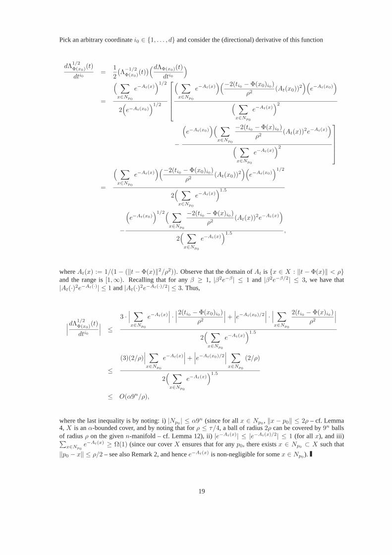
Pick an arbitrary coordinatei0 ∈ 1, . . . , d and consider the (directional) derivative of this function

dΛ1/2Φ(x0)

(t)

dti0=

1

2

(Λ−1/2Φ(x0)

(t))(dΛΦ(x0)(t)

dti0

)

=

( ∑

x∈Np0

e−At(x))1/2

2(

e−At(x0))1/2

( ∑

x∈Np0

e−At(x))(−2(ti0 − Φ(x0)i0)

ρ2(At(x0))

2)(

e−At(x0))

( ∑

x∈Np0

e−At(x))2

−

(

e−At(x0))( ∑

x∈Np0

−2(ti0 − Φ(x)i0)

ρ2(At(x))

2e−At(x))

( ∑

x∈Np0

e−At(x))2

=

( ∑

x∈Np0

e−At(x))(−2(ti0 − Φ(x0)i0)

ρ2(At(x0))

2)(

e−At(x0))1/2

2( ∑

x∈Np0

e−At(x))1.5

−

(

e−At(x0))1/2( ∑

x∈Np0

−2(ti0 − Φ(x)i0)

ρ2(At(x))

2e−At(x))

2( ∑

x∈Np0

e−At(x))1.5 ,

whereAt(x) := 1/(1 − (‖t − Φ(x)‖2/ρ2)). Observe that the domain ofAt is x ∈ X : ‖t − Φ(x)‖ < ρand the range is[1,∞). Recalling that for anyβ ≥ 1, |β2e−β | ≤ 1 and |β2e−β/2| ≤ 3, we have that|At(·)2e−At(·)| ≤ 1 and|At(·)2e−At(·)/2| ≤ 3. Thus,

∣∣∣

dΛ1/2Φ(x0)

(t)

dti0

∣∣∣ ≤

3 ·∣∣∣

∑

x∈Np0

e−At(x)∣∣∣ ·∣∣∣2(ti0 − Φ(x0)i0)

ρ2

∣∣∣+∣∣∣e−At(x0)/2

∣∣∣ ·∣∣∣

∑

x∈Np0

2(ti0 − Φ(x)i0)

ρ2

∣∣∣

2( ∑

x∈Np0

e−At(x))1.5

≤

(3)(2/ρ)∣∣∣

∑

x∈Np0

e−At(x)∣∣∣+∣∣∣e−At(x0)/2

∣∣∣

∑

x∈Np0

(2/ρ)

2( ∑

x∈Np0

e−At(x))1.5

≤ O(α9n/ρ),

where the last inequality is by noting: i)|Np0| ≤ α9n (since for allx ∈ Np0

, ‖x − p0‖ ≤ 2ρ – cf. Lemma4,X is anα-bounded cover, and by noting that forρ ≤ τ/4, a ball of radius2ρ can be covered by9n ballsof radiusρ on the givenn-manifold – cf. Lemma 12), ii)|e−At(x)| ≤ |e−At(x)/2| ≤ 1 (for all x), and iii)∑

x∈Np0e−At(x) ≥ Ω(1) (since our coverX ensures that for anyp0, there existsx ∈ Np0

⊂ X such that

‖p0 − x‖ ≤ ρ/2 – see also Remark 2, and hencee−At(x) is non-negligible for somex ∈ Np0).

19

A.7 Proof of Lemma 7

Note that by definition,‖(DΨ)t(u)‖2 = ‖(DΨ|X|,n)t(u)‖2. Thus, using Eq. (3) and expanding the recur-sion, we have

‖(DΨ)t(u)‖2 = ‖(DΨ|X|,n)t(u)‖2

= ‖(DΨ|X|,n−1)t(u)‖2 + ΛΦ(x|X|)(t)(Cx|X|u)2n + Z|X|,n

...

= ‖(DΨ0,n)t(u)‖2 +[ |X|∑

i=1

ΛΦ(xi)(t)

n∑

j=1

(Cxiu)2j

]

+∑

i,j

Zi,j .

Note that(DΨi,0)t(u) := (DΨi−1,n)t(u). Now recalling that‖(DΨ0,n)t(u)‖2 = ‖u‖2 (the base case of therecursion), all we need to show is that|

∑

i,j Zi,j | ≤ ǫ/2. This follows directly from the lemma below.

Lemma 20 Let ǫ0 ≤ O(ǫ/d(n|X|)2

), and for anyi, j, letωi,j ≥ Ω

((Ki,j + (α9n/ρ))(nd|X|)2/ǫ

)(as per

the statement of Lemma 7). Then, for anyi, j, |Zi,j | ≤ ǫ/2n|X|.Proof: Recall that (cf. Eq. (3))

Zi,j =1

ω2i,j

∑

k

(ζk,4i,j

)2

︸ ︷︷ ︸

(a)

+2∑

k

ζk,4i,j

ωi,j

(ζk,1i,j + ζk,2i,j + ζk,3i,j

)

︸ ︷︷ ︸

(b)

+2∑

k

ζk,1i,j ζk,2i,j

︸ ︷︷ ︸

(c)

+2∑

k

ζk,1i,j ζk,3i,j

︸ ︷︷ ︸

(d)

.

Term (a): Note that|∑

k(ζk,4i,j )

2| ≤ O(d3(Ki,j + (α9n/ρ))2

)(cf. Lemma 21 (iv)). By our choice ofωi,j ,

we have term (a) at mostO(ǫ/n|X|).

Term (b): Note that∣∣ζk,1i,j + ζk,2i,j + ζk,3i,j

∣∣ ≤ O(n|X| + (ǫ/dn|X|)) (by noting Lemma 21 (i)-(iii), recall-

ing the choice ofωi,j , and summing over alli′, j′). Thus,∣∣∑

k ζk,4i,j (ζ

k,1i,j + ζk,2i,j + ζk,3i,j )

∣∣ ≤ O

((d2(Ki,j +

(α9n/ρ)))(n|X|+ (ǫ/dn|X|)

)). Again, by our choice ofωi,j , term (b) is at mostO(ǫ/n|X|).

Terms (c) and (d):We focus on bounding term (c) (the steps for bounding term (d)are same). Note that|∑

k ζk,1i,j ζ

k,2i,j | ≤ 4|

∑

k ζk,1i,j (ηi,j(t))k|. Now, observe that

(ζk,1i,j

)

k=1,...,2d+3is a tangent vector with length

at mostO(dn|X| + (ǫ/dn|X|)) (cf. Lemma 21 (i)). Thus, by noting thatηi,j is almost normal (with qualityof approximationǫ0), we have term (c) at mostO(ǫ/n|X|).

By choosing the constants in the order terms appropriately,we can get the lemma.

Lemma 21 Let ζk,1i,j , ζk,2i,j , ζk,3i,j , andζk,4i,j be as defined in Eq.(3). Then for all1 ≤ i ≤ |X| and1 ≤ j ≤ n,we have

(i) |ζk,1i,j | ≤ 1 + 8n|X|+∑i

i′=1

∑j−1j′=1O(d(Ki′,j′ + (α9n/ρ))/ωi′,j′),

(ii) |ζk,2i,j | ≤ 4,

(iii) |ζk,3i,j | ≤ 4,

(iv) |ζk,4i,j | ≤ O(d(Ki,j + (α9n/ρ))).

Proof: First note for any‖u‖ ≤ 1 and for anyxi ∈ X, 1 ≤ j ≤ n and1 ≤ l ≤ d, we have|∑l Cxi

j,lul| =|(Cxiu)j | ≤ 4 (cf. Lemma 23 (b) and Corollary 5).

Noting that for alli andj, ‖ηi,j‖ = ‖νi,j‖ = 1, we have|ζ2,ki,j | ≤ 4 and|ζ3,ki,j | ≤ 4.

Observe thatζk,4i,j =∑

l ulRk,li,j . For all i, j, k andl, note that i)‖dηi,j(t)/dtl‖ ≤ Ki,j and‖dνi,j(t)/dtl‖ ≤

Ki,j and ii) |dλ1/2Φ(xi)(t)/dtl| ≤ O(α9n/ρ) (cf. Lemma 19). Thus we have|ζk,4i,j | ≤ O(d(Ki,j + (α9n/ρ))).

Now for any i, j, note thatζk,1i,j =∑

l uldΨi,j−1(t)/dtl. Thus by recursively expanding,|ζk,1i,j | ≤ 1 +

8n|X|+∑ii′=1

∑j−1j′=1O(d(Ki′,j′ + (α9n/ρ))/ωi′,j′).

20

A.8 Proof of Lemma 8

We start by stating the following useful observations:

Lemma 22 LetA be a linear operator such thatmax‖x‖=1 ‖Ax‖ ≤ δmax. Letu be a unit-length vector. If‖Au‖ ≥ δmin > 0, then for any unit-length vectorv such that|u · v| ≥ 1− ǫ, we have

1− δmax

√2ǫ

δmin≤ ‖Av‖‖Au‖ ≤ 1 +

δmax

√2ǫ

δmin.

Proof: Let v′ = v if u ·v > 0, otherwise letv′ = −v. Quickly note that‖u−v′‖2 = ‖u‖2+‖v′‖2−2u ·v′ =2(1− u · v′) ≤ 2ǫ. Thus, we have,

i. ‖Av‖ = ‖Av′‖ ≤ ‖Au‖+ ‖A(u− v′)‖ ≤ ‖Au‖+ δmax

√2ǫ,

ii. ‖Av‖ = ‖Av′‖ ≥ ‖Au‖ − ‖A(u− v′)‖ ≥ ‖Au‖ − δmax

√2ǫ.

Noting that‖Au‖ ≥ δmin yields the result.

Lemma 23 Let x1, . . . , xn ∈ RD be a set of orthonormal vectors,F := [x1, . . . , xn] be aD × n matrix

and letΦ be a linear map fromRD to Rd (n ≤ d ≤ D) such that for all non-zeroa ∈ span(F ) we have

0 < ‖Φa‖ ≤ ‖a‖. LetUΣV T be the thin SVD ofΦF . DefineC = (Σ−2 − I)1/2UT. Then,

(a) ‖C(Φa)‖2 = ‖a‖2 − ‖Φa‖2, for anya ∈ span(F ),

(b) ‖C‖2 ≤ (1/σn)2, where‖ · ‖ denotes the spectral norm of a matrix andσn is thenth largest singularvalue ofΦF .

Proof: Note thatFV forms an orthonormal basis for the subspace spanned by columns ofF that maps toUΣ via the mappingΦ. Thus, sincea ∈ span(F ), let y be such thata = FV y. Note that i)‖a‖2 = ‖y‖2, ii)‖Φa‖2 = ‖UΣy‖2 = yTΣ2y. Now,

‖CΦa‖2 = ‖((Σ−2 − I)1/2UT)ΦFV y‖2

= ‖(Σ−2 − I)1/2UTUΣV TV y‖2

= ‖(Σ−2 − I)1/2Σy‖2

= yTy − yTΣ2y

= ‖a‖2 − ‖Φa‖2.Now, consider‖C‖2.

‖C‖2 ≤ ‖(Σ−2 − I)1/2‖2‖UT‖2

≤ max‖x‖=1

‖(Σ−2 − I)1/2x‖2

≤ max‖x‖=1

xTΣ−2x

= max‖x‖=1

∑

i

x2i /(σi)2

≤ (1/σn)2,

whereσi are the (topn) singular values forming the diagonal matrixΣ.

Lemma 24 Let M ⊂ RD be a compact Riemanniann-manifold with condition number1/τ . Pick any

x ∈ M and letFx be anyn-dimensional affine space with the property: for any unit vector vx tangent toMatx, and its projectionvxF ontoFx,

∣∣vx · vxF

‖vxF ‖

∣∣ ≥ 1−δ. Then for anyp ∈M such that‖x−p‖ ≤ ρ ≤ τ/2,

and any unit vectorv tangent toM at p, (ξ := (2ρ/τ) + δ + 2√

2ρδ/τ )

i.∣∣∣v · vF

‖vF ‖

∣∣∣ ≥ 1− ξ,

ii. ‖vF ‖2 ≥ 1− 2ξ,

21

iii. ‖vr‖2 ≤ 2ξ,

wherevF is the projection ofv ontoFx andvr is the residual (i.e.v = vF + vr andvF⊥vr).

Proof: Let γ be the angle betweenvF andv. We will bound this angle.Let vx (atx) be the parallel transport ofv (atp) via the (shortest) geodesic path via the manifold connec-

tion. Let the angle between vectorsv andvx beα. Let vxF be the projection ofvx onto the subspaceFx,and let the angle betweenvx andvxF beβ. WLOG, we can assume that the anglesα andβ are acute. Then,

sinceγ ≤ α + β ≤ π, we have that∣∣∣v · vF

‖vF ‖

∣∣∣ = cos γ ≥ cos(α + β). We bound the individual termscosα

andcosβ as follows.Now, since‖p − x‖ ≤ ρ, using Lemmas 9 and 10, we havecos(α) = |v · vx| ≥ 1 − 2ρ/τ . We also

havecos(β) =∣∣∣vx · vxF

‖vxF ‖

∣∣∣ ≥ 1 − δ. Then, using Lemma 16, we finally get

∣∣∣v · vF

‖vF ‖

∣∣∣ = | cos(γ)| ≥

1− 2ρ/τ − δ − 2√

2ρδ/τ = 1− ξ.Also note since1 = ‖v‖2 = (v · vF

‖vF ‖ )2∥∥∥

vF

‖vF ‖

∥∥∥

2

+ ‖vr‖2, we have‖vr‖2 = 1−(

v · vF

‖vF ‖

)2

≤ 2ξ, and

‖vF ‖2 = 1− ‖vr‖2 ≥ 1− 2ξ.

Now we are in a position to prove Lemma 8. LetvF be the projection of the unit vectorv (atp) onto thesubspace spanned by (the columns of)Fx andvr be the residual (i.e.v = vF + vr andvF⊥vr). Then, notingthatp, x, v andFx satisfy the conditions of Lemma 24 (withρ in the Lemma 24 replaced with2ρ from thestatement of Lemma 8), we have (ξ := (4ρ/τ) + δ + 4

√

ρδ/τ )

a)∣∣v · vF

‖vF ‖

∣∣ ≥ 1− ξ,

b) ‖vF ‖2 ≥ 1− 2ξ,

c) ‖vr‖2 ≤ 2ξ.

We can now bound the required quantity‖Cxu‖2. Note that

‖Cxu‖2 = ‖CxΦv‖2 = ‖CxΦ(vF + vr)‖2

= ‖CxΦvF ‖2 + ‖CxΦvr‖2 + 2CxΦvF · CxΦvr

= ‖vF ‖2 − ‖ΦvF ‖2︸ ︷︷ ︸

(a)

+ ‖CxΦvr‖2︸ ︷︷ ︸

(b)

+2CxΦvF · CxΦvr︸ ︷︷ ︸

(c)

where the last equality is by observingvF is in the span ofFx and applying Lemma 23 (a). We now boundthe terms(a),(b), and(c) individually.

Term (a): Note that1 − 2ξ ≤ ‖vF ‖2 ≤ 1 and observing thatΦ satisfies the conditions of Lemma 22with δmax = (2/3)

√

D/d, δmin = (1/2) ≤ ‖Φv‖ (cf. Lemma 4) and∣∣v · vF

‖vF ‖

∣∣ ≥ 1 − ξ, we have (recall

‖Φv‖ = ‖u‖ ≤ 1)

‖vF ‖2 − ‖ΦvF ‖2 ≤ 1− ‖vF ‖2∥∥∥∥Φ

vF‖vF ‖

∥∥∥∥

2

≤ 1− (1− 2ξ)

∥∥∥∥Φ

vF‖vF ‖

∥∥∥∥

2

≤ 1 + 2ξ −∥∥∥∥Φ

vF‖vF ‖

∥∥∥∥

2

≤ 1 + 2ξ −(1− (4/3)

√

2ξD/d)2 ‖Φv‖2

≤ 1− ‖u‖2 +(2ξ + (8/3)

√

2ξD/d), (7)

where the fourth inequality is by using Lemma 22. Similarly,in the other direction

‖vF ‖2 − ‖ΦvF ‖2 ≥ 1− 2ξ − ‖vF ‖2∥∥∥∥Φ

vF‖vF ‖

∥∥∥∥

2

≥ 1− 2ξ −∥∥∥∥Φ

vF‖vF ‖

∥∥∥∥

2

≥ 1− 2ξ −(1 + (4/3)

√

2ξD/d)2 ‖Φv‖2

≥ 1− ‖u‖2 −(2ξ + (32/9)ξ(D/d) + (8/3)

√

2ξD/d). (8)

22

R2d+3

N = Rd

ΦM

Φp

Φx1

Φx2

Φx3

Φx4

Figure 7:Basic setup for computing the normals to the underlyingn-manifoldΦM at the point of interestΦp. Observethat even though it is difficult to find vectors normal toΦM atΦp within the containing spaceRd (because we only havea finite-size sample fromΦM , viz. Φx1, Φx2, etc.), we can treat the pointΦp as part of the bigger ambient manifoldN(= R

d, that containsΦM ) and compute the desired normals in a space that containsN itself. Now, for eachi, j iterationof Algorithm II, Ψi,j acts on the entireN , and since we have complete knowledge aboutN , we can compute the desirednormals.

Term (b): Note that for anyx, ‖Φx‖ ≤ (2/3)(√

D/d)‖x‖. We can apply Lemma 23 (b) withσnx ≥ 1/4 (cf.

Corollary 5) and noting that‖vr‖2 ≤ 2ξ, we immediately get

0 ≤ ‖CxΦvr‖2 ≤ 42 · (4/9)(D/d)‖vr‖2 ≤ (128/9)(D/d)ξ. (9)

Term (c): Recall that for anyx, ‖Φx‖ ≤ (2/3)(√

D/d)‖x‖, and using Lemma 23 (b) we have that‖Cx‖2 ≤16 (sinceσn

x ≥ 1/4 – cf. Corollary 5).Now let a := CxΦvF and b := CxΦvr. Then‖a‖ = ‖CxΦvF ‖ ≤ ‖Cx‖‖ΦvF ‖ ≤ 4, and‖b‖ =

‖CxΦvr‖ ≤ (8/3)√

2ξD/d (see Eq. (9)).

Thus,|2a · b| ≤ 2‖a‖‖b‖ ≤ 2 · 4 · (8/3)√

2ξD/d = (64/3)√

2ξD/d. Equivalently,

−(64/3)√

2ξD/d ≤ 2CxΦvF · CxΦvr ≤ (64/3)√

2ξD/d. (10)

Combining (7)-(10), and notingd ≤ D, yields the lemma.

A.9 Computing the Normal Vectors

The success of the second embedding technique crucially depends upon finding (at each iteration step) a pairof mutually orthogonal unit vectors that are normal to the embedding of manifoldM (from the previousiteration step) at a given pointp. At a first glance finding such normal vectors seems infeasible since weonly have access to a finite size sampleX fromM . The saving grace comes from noting that the correctionsare applied to then-dimensional manifoldΦ(M) that is actually asubmanifoldof d-dimensional spaceRd.Let’s denote this spaceRd as a flatd-manifoldN (containing our manifold of interestΦ(M)). Note thateven though we only have partial information aboutΦ(M) (since we only have samples from it), we havefull information aboutN (since it is the entire spaceRd). What it means is that given some point of interestΦp ∈ Φ(M) ⊂ N , finding a vector normal toN (atΦp) automatically is a vector normal toΦ(M) (atΦp).Of course, to find two mutually orthogonal normals to ad-manifoldN , N itself needs to be embedded in alarger dimensional Euclidean space (although embedding into d+2 should suffice, for computational reasonswe will embedN into Euclidean space of dimension2d + 3). This is precisely the first thing we do beforeapplying any corrections (cf. Step 2 of Embedding II in Section 4). See Figure 7 for an illustration of thesetup before finding any normals.

Now for every iteration of the algorithm, note that we have complete knowledge ofN and exactly whatfunction (namelyΨi,j for iterationi, j) is being applied toN . Thus with additional computation effort, onecan compute the necessary normal vectors.

More specifically, We can estimate a pair of mutually orthogonal unit vectors that are normal toΨi,j(N)atΦp (for any stepi, j) as follows.

23

Algorithm 4 Compute Normal VectorsPreprocessing Stage:1: Let ηrand

i,j andνrandi,j be vectors inR2d+3 drawn independently at random from the surface of the unit-sphere

(for 1 ≤ i ≤ |X|, 1 ≤ j ≤ n).

Compute Normals: For any point of interestp ∈M , let t := Φp denote its projection intoRd. Now, for anyiterationi, j (where1 ≤ i ≤ |X|, and1 ≤ j ≤ n), we shall assume that vectorsη andν upto iterationsi, j−1are already given. Then we can compute the (approximated) normalsηi,j(t) andνi,j(t) for the iterationi, jas follows.1: Let∆ > 0 be the quality of approximation.2: for k = 1, . . . , d do3: Approximate thekth tangent vector as

T k :=Ψi,j−1(t+∆ek)−Ψi,j−1(t)

∆,

whereΨi,j−1 is as defined in Section 5.3, andek is thekth standard vector.4: end for5: Let η = ηrand

i,j , andν = νrandi,j .

6: Use Gram-Schmidt orthogonalization process to extractη (from η) that is orthogonal to vectorsT 1, . . . , T d.

7: Use Gram-Schmidt orthogonalization process to extractν (from ν) that is orthogonal to vectorsT 1, . . . , T d, η.

8: return η/‖η‖ and ν/‖ν‖ as mutually orthogonal unit vectors that are approximatelynormal toΨi,j−1(ΦM) atΨi,j−1(t).

A few remarks are in order.

Remark 7 The choice of target dimension of size2d + 3 (instead ofd + 2) ensures that a pair of randomunit-vectorsη andν are not parallel to any vector in the tangent bundle ofΨi,j−1(N) with probability1. Thisagain follows from Sard’s theorem, and is the key observation in reducing the embedding size in Whitney’sembedding [Whi36]. This also ensures that our orthogonalization process (Steps 6 and 7) will not result in anull vector.

Remark 8 By picking∆ sufficiently small, we can approximate the normalsη and ν arbitrarily well byapproximating the tangentsT 1, . . . , T d well.

Remark 9 For each iterationi, j, the vectorsη/‖η‖ and ν/‖ν‖ that are returned (in Step 8) are a smoothmodification to the starting vectorsηrand

i,j andνrandi,j respectively. Now, since we use the same starting vectors

ηrandi,j and νrand

i,j regardless of the point of application (t = Φp), it follows that the respective directionalderivates of the returned vectors are bounded as well.

By noting Remarks 8 and 9, the approximate normals we return satisfy the conditions needed for Embed-ding II (see our discussion in Section 5.3).

24