To appear in EPTCS.c©M. Benerecetti, M. Faella & S. Minopoli

This work is licensed under theCreative Commons Attribution License.

Towards Efficient Exact Synthesis for Linear Hybrid Systems

Massimo Benerecetti Marco FaellaUniversita di Napoli“Federico II”, Italy

{mfaella,bene,minopoli}@na.infn.it

Stefano Minopoli

We study the problem of automatically computing the controllable region of a Linear Hybrid Au-tomaton, with respect to a safety objective. We describe the techniques that are needed to effectivelyand efficiently implement a recently-proposed solution procedure, based on polyhedral abstractionsof the state space. Supporting experimental results are presented, based on an implementation of theproposed techniques on top of the tool PHAVer.

1 Introduction

Hybrid systems are an established formalism for modeling physical systems which interact with a digitalcontroller. From an abstract point of view, a hybrid system is a dynamic system whose state variables areboth discrete and continuous. Typically, continuous variables represent physical quantities like tempera-ture, speed, etc., while discrete ones represent control modes, i.e., states of the controller.

Hybrid automata [11] are the most common syntactic variety of hybrid system: a finite set of loca-tions, similar to the states of a finite automaton, represents the value of the discrete variables. The currentlocation, together with the current value of the (continuous) variables, form the instantaneous descriptionof the system. Change of location happens via discrete transitions, and the evolution of the variables isgoverned by differential equations attached to each location. In a Linear Hybrid Automaton (LHA), theallowed differential equations are in fact polyhedral differential inclusions of the type x ∈ P, where x isthe vector of the first derivatives of all variables and P is a convex polyhedron. Notice that differentialinclusions are non-deterministic, allowing for infinitely many solutions.

We study LHAs whose discrete transitions are partitioned into controllable and uncontrollable ones,and we wish to compute a strategy for the controller to satisfy a given goal, regardless of the evolutionof the continuous variables and of the uncontrollable transitions. Hence, the problem can be viewed as atwo player game: on one side the controller, who can only issue controllable transitions, on the other sidethe environment, who can choose the trajectory of the variables and can take uncontrollable transitionsat any moment.

As control goal, we consider safety, i.e., the objective of keeping the system within a given region ofsafe states. This problem has been considered several times in the literature. In [6], we fixed some inac-curacies in previous presentations, and proposed a sound and complete semi-procedure for the problem.Here, we discuss the techniques required to efficiently implement the algorithms in [6]. In particular,two operators on polyhedra need non-trivial new developments to be exactly and efficiently computed.Both operators pertain to intra-location behavior, and therefore assume that trajectories are subject to afixed polyhedral differential inclusion of the type x ∈ P.

• The pre-flow operator. Given a polyhedron U ⊆ Rn, we wish to compute the set of all points thatmay reach U via an admissible trajectory. This apparently easy task becomes non-trivial when theconvex polyhedron P is not (necessarily) topologically closed. This is the topic of Section 4.

2 Towards Efficient Exact Synthesis for Linear Hybrid Systems

• The may reach while avoiding operator, denoted by RWAm. Given two polyhedra U and V , theoperator computes the set of points that may reach U while avoiding V , via an admissible trajectory.A fixpoint algorithm for this operator was presented in [6]. Here, we introduce a number ofefficiency improvements (Section 5), accompanied by a corresponding experimental evaluation(Section 6), carried out on our tool PHAVer+, based on the open-source tool PHAVer [9].

Contrary to most recent literature on the subject, we focus on exact algorithms. Although it is establishedthat exact analysis and synthesis of realistic hybrid systems is computationally demanding, we believethat the ongoing research effort on approximate techniques should be based on the solid grounds providedby the exact approach. For instance, a tool implementing an exact algorithm (like our PHAVer+) mayserve as a benchmark to evaluate the performance and the precision of an approximate tool.

Related work. The idea of automatically synthesizing controllers for dynamic systems first arose inconnection with discrete systems [17]. Then, the same idea was applied to real-time systems modeledby timed automata [16], thus coming one step closer to the continuous systems that control theory usu-ally deals with. Finally, it was the turn of hybrid systems [20, 13], and in particular of LHA, the verymodel that we analyze in this paper. Wong-Toi proposed the first symbolic semi-procedure to computethe controllable region of a LHA w.r.t. a safety goal [20]. The heart of the procedure lies in the oper-ator flow avoid(U,V ), which is analogous to our RWAm. However, the algorithm provided in [20] forflow avoid does not work for non-convex V , a case which is very likely to occur in practice, even if theoriginal safety goal is convex. A revised algorithm, correcting such flaw, was proposed in [6].

Tomlin et al. and Balluchi et al. analyze much more expressive models [18, 5], with generality in mindrather than automatic synthesis. Their Reach and Unavoid Pre operators, respectively, again correspondto RWAm.

Asarin et al. investigate the synthesis problem for hybrid systems where all discrete transitions arecontrollable and the trajectories satisfy given linear differential equations of the type x = Ax [2]. Theexpressive power of these constraints is incomparable with the one offered by the differential inclusionsoccurring in LHAs. In particular, linear differential equations give rise to deterministic trajectories,while differential inclusions are non-deterministic. In control theory terms, differential inclusions canrepresent the presence of environmental disturbances. The tool d/dt [3], by the same authors, is reportedto support controller synthesis for safety objectives, but the publicly available version in fact does not.

2 Linear Hybrid Automata

A convex polyhedron is a subset of Rn that is the intersection of a finite number of half-spaces. Apolyhedron is a subset of Rn that is the union of a finite number of convex polyhedra. For a general (i.e.,not necessarily convex) polyhedron G⊆ Rn, we denote by [[G]]⊆ 2R

nthe finite set of convex polyhedra

comprising it.Given an ordered set X = {x1, . . . ,xn} of variables, a valuation is a function v : X → R. Let Val(X)

denote the set of valuations over X . There is an obvious bijection between Val(X) and Rn, allowing us toextend the notion of (convex) polyhedron to sets of valuations. We denote by CPoly(X) (resp., Poly(X))the set of convex polyhedra (resp., polyhedra) on X .

We use X to denote the set {x1, . . . , xn} of dotted variables, used to represent the first derivatives, andX ′ to denote the set {x′1, . . . ,x′n} of primed variables, used to represent the new values of variables after atransition. Arithmetic operations on valuations are defined in the straightforward way. An activity overX is a differentiable function f : R≥0 → Val(X). Let Acts(X) denote the set of activities over X . The

M. Benerecetti, M. Faella & S. Minopoli 3

derivative f of an activity f is defined in the standard way and it is an activity over X . A Linear HybridAutomaton H = (Loc,X ,Edgc,Edgu,Flow, Inv, Init) consists of the following:

• A finite set Loc of locations.

• A finite set X = {x1, . . . ,xn} of continuous, real-valued variables. A state is a pair (l,v) of alocation l and a valuation v ∈ Val(X).

• Two sets Edgc and Edgu of controllable and uncontrollable transitions, respectively. They describeinstantaneous changes of locations, in the course of which variables may change their value. Eachtransition (l,µ, l′) ∈ Edgc ∪Edgu consists of a source location l, a target location l′, and a jumprelation µ ∈ Poly(X ∪ X ′), that specifies how the variables may change their value during thetransition. The projection of µ on X describes the valuations for which the transition is enabled;this is often referred to as a guard.

• A mapping Flow : Loc→ CPoly(X) attributes to each location a set of valuations over the firstderivatives of the variables, which determines how variables can change over time.

• A mapping Inv : Loc→ Poly(X), called the invariant.

• A mapping Init : Loc→ Poly(X), contained in the invariant,, which allows the definition of theinitial states from which all behaviors of the automaton originate.

We use the abbreviations S = Loc×Val(X) for the set of states and Edg = Edgc∪Edgu for the set of alltransitions. Moreover, we let InvS =

⋃l∈Loc{l}× Inv(l) and InitS =

⋃l∈Loc{l}× Init(l). Notice that InvS

and InitS are sets of states.

2.1 Semantics

The behavior of a LHA is based on two types of transitions: discrete transitions correspond to the Edgcomponent, and produce an instantaneous change in both the location and the variable valuation; timedtransitions describe the change of the variables over time in accordance with the Flow component.

Given a state s = 〈l,v〉, we set loc(s) = l and val(s) = v. An activity f ∈ Acts(X) is called admissiblefrom s if (i) f (0) = v and (ii) for all δ ≥ 0 it holds f (δ ) ∈ Flow(l). We denote by Adm(s) the setof activities that are admissible from s. Additionally, for f ∈ Adm(s), the span of f in l, denoted byspan( f , l) is the set of all values δ ≥ 0 such that 〈l, f (δ ′)〉 ∈ InvS for all 0 ≤ δ ′ ≤ δ . Intuitively, δ is inthe span of f iff f never leaves the invariant in the first δ time units. If all non-negative reals belong tospan( f , l), we write ∞ ∈ span( f , l).

Runs. Given two states s,s′, and a transition e ∈ Edg, there is a discrete transition s e−→ s′ with source sand target s′ iff (i) s,s′ ∈ Invs, (ii) e = (loc(s),µ, loc(s′)), and (iii) (val(s),val(s′)′) ∈ µ , where val(s′)′

is the valuation over X ′ obtained from val(s′) by renaming each variable x ∈ X onto the corresponding

primed variable x′ ∈X . There is a timed transition sδ , f−−→ s′ with duration δ ∈R≥0 and activity f ∈Adm(s)

iff (i) s ∈ Invs, (ii) δ ∈ span( f , loc(s)), and (iii) s′ = 〈loc(s), f (δ )〉. For technical convenience, we admit

timed transitions of duration zero1. A special timed transition is denoted s∞, f−−→ and represents the case

when the system follows an activity forever. This is only allowed if ∞ ∈ span( f , loc(s)). Finally, a joint

transition sδ , f ,e−−−→ s′ represents the timed transition s

δ , f−−→〈loc(s), f (δ )〉 followed by the discrete transition〈loc(s), f (δ )〉 e−→ s′.

1Timed transitions of duration zero can be disabled by adding a clock variable t to the automaton and requesting that eachdiscrete transition happens when t > 0 and resets t to 0 when taken.

4 Towards Efficient Exact Synthesis for Linear Hybrid Systems

A run is a sequence

r = s0δ0, f0−−→ s′0

e0−→ s1δ1, f1−−→ s′1

e1−→ s2 . . .sn . . . (1)

of alternating timed and discrete transitions, such that either the sequence is infinite, or it ends with a

timed transition of the type sn∞, f−−→. If the run r is finite, we define len(r) = n to be the length of the

run, otherwise we set len(r) = ∞. The above run is non-Zeno if for all δ ≥ 0 there exists i≥ 0 such that∑

ij=0 δ j > δ . We denote by States(r) the set of all states visited by r. Formally, States(r) is the set of

states 〈loc(si), fi(δ )〉, for all 0≤ i≤ len(r) and all 0≤ δ ≤ δi. Notice that the states from which discretetransitions start (states s′i in (1)) appear in States(r). Moreover, if r contains a sequence of one or morezero-time timed transitions, all intervening states appear in States(r).

Zenoness and well-formedness. A well-known problem of real-time and hybrid systems is that defi-nitions like the above admit runs that take infinitely many discrete transitions in a finite amount of time(i.e., Zeno runs), even if such behaviors are physically meaningless. In this paper, we assume that thehybrid automaton under consideration generates no such runs. This is easily achieved by using an extravariable, representing a clock, to ensure that the delay between any two transitions is bounded from be-low by a constant. We leave it to future work to combine our results with more sophisticated approachesto Zenoness known in the literature [5, 1].

Moreover, we assume that the hybrid automaton under consideration is non-blocking, i.e., wheneverthe automaton is about to leave the invariant there must be an uncontrollable transition enabled. If ahybrid automaton is non-Zeno and non-blocking, we say that it is well-formed. In the following, allhybrid automata are assumed to be well-formed.

Strategies. A strategy is a function σ : S→ 2Edgc∪{⊥} \ /0, where ⊥ denotes the null action. Noticethat our strategies are non-deterministic and memoryless (or positional). A strategy can only choose atransition which is allowed by the automaton. Formally, for all s ∈ S, if e ∈ σ(s)∩Edgc, then thereexists s′ ∈ S such that s e−→ s′. Moreover, when the strategy chooses the null action, it should continueto do so for a positive amount of time, along each activity that remains in the invariant. If all activitiesimmediately exit the invariant, the above condition is vacuously satisfied. This ensures that the nullaction is enabled in right-open regions, so that there is an earliest instant in which a controllable transitionbecomes mandatory.

Notice that a strategy can always choose the null action. The well-formedness condition ensures thatthe system can always evolve in some way, be it a timed step or an uncontrollable transition. In particular,even if we are on the boundary of the invariant we allow the controller to choose the null action, because,in our interpretation, it is not the responsibility of the controller to ensure that the invariant is not violated.

We say that a run like (1) is consistent with a strategy σ if for all 0 ≤ i < len(r) the followingconditions hold:

• for all δ ≥ 0 such that ∑i−1j=0 δ j ≤ δ < ∑

ij=0 δ j, we have ⊥ ∈ σ(〈loc(si), fi(δ −∑

i−1j=0 δ j)〉);

• if ei ∈ Edgc then ei ∈ σ(s′i).

We denote by Runs(s,σ) the set of runs starting from the state s and consistent with the strategy σ .

Safety control problem. Given a hybrid automaton and a set of states T ⊆ InvS, the safety controlproblem asks whether there exists a strategy σ such that, for all initial states s ∈ InitS, all runs r ∈Runs(s,σ) it holds States(r)⊆ T .

M. Benerecetti, M. Faella & S. Minopoli 5

3 Solving the Safety Control Problem

In this section, we recall the semi-procedure that solves the safety control problem for a given LHAand safe region. It is well known in the literature (see e.g. [15, 2]) that the answer to the safety controlproblem for safe set T ⊆ Inv is positive if and only if

Init ⊆ νW .T ∩CPre(W ),

where CPre is the controllable predecessor operator, defined below. Since the reachability problem forLHA was proved undecidable [14], the above fixpoint may not converge in a finite number of steps. Onthe other hand, it does converge in many cases of practical interest, as witnessed by the examples inSection 6.

For a set of states A, the operator CPre(A) returns the set of states from which the controller canensure that the system remains in A during the next joint transition. This happens if for all activitieschosen by the environment and all delays δ , one of two situations occurs:• either the systems stays in A up to time δ , while all uncontrollable transitions enabled up to time

δ (included) also lead to A, or

• some preceding instant δ ′ < δ exists such that the system stays in A up to time δ ′, while alluncontrollable transitions enabled up to time δ ′ (included) also lead to A, and the controller canissue a transition at time δ ′ leading to A.

In order to compute CPre(A) on LHA, the auxiliary operator RWAm (may reach while avoiding) wasproposed [6]. Intuitively, given a location l and two sets of variable valuations U and V , RWAm

l (U,V )contains the set of valuations from which the continuous evolution of the system may reach U whileavoiding V ∩U .

For a set of states A and x∈ {u,c}, let Premx (A) (for may predecessors) be the set of states where some

discrete transition leading to A and belonging to Edgx is enabled. We denote with A�l the projection of Aon l, i.e. {v ∈ Val(X) | 〈l,v〉 ∈ A}. As proved in [6], we then have that

CPre(A) =⋃

l∈Loc

{l}×(

A�l \RWAml(Inv(l)∩

(A�l ∪Bl

),Cl ∪ Inv(l)

)),

where Bl = Premu(A)�l and Cl = Prem

c (A)�l .Intuitively, the set Bl is the set of valuations u such that from state 〈l,u〉 the environment can take a

discrete transition leading outside A, and Cl is the set of valuations u such that from 〈l,u〉 the controllercan take a discrete transition into A. Then, using the RWAm operator, we compute the set of valuationsfrom which there exists an activity that either leaves A or enters Bl , while staying in the invariant andavoiding Cl . These valuations do not belong to CPre(A), as the environment can violate the safety goalwithin (at most) one discrete transition.

Next, we show how to characterize RWAm in terms of simple operations on polyhedra. Let cl(P)denote the topological closure of a polyhedron P. Given two polyhedra P and F , the pre-flow of P w.r.t.F is:

P↙F = {x−δy | x ∈ P,y ∈ F,δ ≥ 0}.For a given location l ∈ Loc, the pre-flow of P w.r.t. Flow(l) is the set of points that can reach P via astraight-line activity whose slope is allowed in l. For notational convenience, we use the abbreviationP↙l for P↙Flow(l), and for all polyhedra P and P′ we define their boundary to be

bndry(P,P′) = (cl(P)∩P′)∪ (P∩ cl(P′)),

6 Towards Efficient Exact Synthesis for Linear Hybrid Systems

which identifies a boundary between two (not necessarily closed) convex polyhedra. Clearly, bndry(P,P′)is not empty only if P and P′ are adjacent to one another or if they overlap; it is empty, otherwise.Moreover, given a location l, entry(P,P′), the entry region between P and P′, denotes the set of points ofthe boundary between P and P′ which can reach P′ by following some straight-line activity in location l.In symbols: entry(P,P′) = bndry(P,P′)∩P′↙l . The following theorem gives a fixpoint characterizationof RWAm.Theorem 1 ([6]) For all locations l and polyhedra U, V , it holds

RWAml (U,V ) = µW .U ∪

⋃P∈[[V ]]

⋃P′∈[[W ]]

(P∩ entry(P,P′)↙l

). (2)

The equation refines the under-approximation U by identifying its entry regions, i.e., the boundariesbetween the area which may belong to the result (i.e., V ), and the area which already belongs to it (i.e.,W ). Figure 1 shows a single step in the computation of equation 2, for a fixed pair of convex polyhedraP in V and P′ in W . Dashed lines represent topologically open sides. The dark gray rectangles representconvex polyhedra in W , while the light gray one is P.

In Figure 1(a) the thick segment between P and P′ represents bndry(P,P′) and, in the example, iscontained in P. Since P′ is topologically open (denoted by the dashed line), the rightmost point ofbndry(P,P′) cannot reach P′ along any straight-line activity. Being P′ open, so is P′↙l , and its inter-section with P, namely entry(P,P′), does not contain the rightmost point of the boundary (Figure 1(b)).Now, any point of P that can reach entry(P,P′) following some activity can also reach P′, and the setCut = P∩ entry(P,P′)↙l contains precisely those points (Figure 1(c) and Figure 1(d)). All these pointsmust then be added to W , as they all belong to RWAm

l (U,V ).

P′

P

(a) Initial input,with bndry(P,P′)highlighted.

P′

P

P′ ↙

(b) Pre-flow of P′.

P ′ ↙entry(P,P′)↙P

P′

(c) Entry region.

Pnew

Cut

P′

(d) Pnew, Cut. (e)Flow(l).

Figure 1: Algorithm behavior.

In our implementation, instead of computing the operator RWAml , we compute the dual operator

SORMl (Z,V ) (for must stay or reach), containing the points which either remain in Z forever or reach V

along a system trajectory that does not leave Z. The operator SORMl can be defined as follows:

SORMl (Z,V ) = RWAm

l (Z,V ). (3)

As a consequence, we can compute CPre(A) as⋃l∈Loc

{l}×(

A�l ∩SORMl(Inv�l ∪

(A�l \Bl

),Cl ∪ Inv�l

)).

M. Benerecetti, M. Faella & S. Minopoli 7

From (3), we obtain a fixpoint characterization of the operator SORMl :

SORMl (Z,V ) = RWAm

l (Z,V ) = µW .Z∪⋃

P∈[[V ]]

⋃P′∈[[W ]]

(P∩ entry(P,P′)↙l

)=

= νW .Z∩⋃

P∈[[V ]]

⋃P′∈[[W ]]

(P∩ entry(P,P′)↙l

)= νW .Z \

⋃P∈[[V ]]

⋃P′∈[[W ]]

(P∩ entry(P,P′)↙l

). (4)

The following two sections show how to effectively and efficiently compute fixpoint (4).

4 Exact Computation of Pre-Flow

As seen in the previous section, one of the basic operations on polyhedra that are needed to computeSORM is the pre-flow operator↙. It is sufficient to compute P↙F for convex P and F , for two reasons:First, we always have F = Flow(l), for a given location l, and Flow(l) is a convex polyhedron by as-sumption. Second, (P1∪P2)↙F = (P1↙F)∪ (P2↙F), so the pre-flow of a general polyhedron is theunion of the pre-flows of its convex polyhedra.The pre-flow of P w.r.t. F is equivalent to the post-flow of P w.r.t. −F , defined as:

P↗−F = {x+δ · y | x ∈ P,y ∈ −F,δ ≥ 0}.

The post-flow operation coincides with the time-elapse operation introduced in [10] for topologicallyclosed convex polyhedra. Notice that for convex polyhedra P and F , the post-flow of P w.r.t. F may notbe a convex polyhedron: following [2], let P⊆R2 be the polyhedron containing only the origin (0,0) andlet F be defined by the constraint y > 0. We have P↗F = {(0,0)}∪{(x,y) ∈R2 | y > 0}, which is not aconvex polyhedron (although it is a convex subset of R2). The Parma Polyhedral Library (PPL, see [4]),for instance, only provides an over-approximation P↗PPL F of the post-flow P↗F , as the smallest convexpolyhedron containing P↗F .

On the other hand, the post-flow of a convex polyhedron is always the union of two convex polyhedra,according to the equation

P↗F = P∪(P↗>0 F

),

where P↗>0 F is the positive post-flow of P, i.e., the set of valuations that can be reached from P via astraight line of non-zero length whose slope belongs to F . Formally,

P↗>0 F = {x+δ · y | x ∈ P,y ∈ F,δ > 0}.

Hence, in order to exactly compute the post-flow of a convex polyhedron, we show how to compute thepositive post-flow.

Convex polyhedra admit two finite representations, in terms of constraints or generators. Librarieslike PPL maintain both representations for each convex polyhedron and efficient algorithms exist forkeeping them synchronized [7, 19]. The constraint representation refers to the set of linear inequalitieswhose solutions are the points of the polyhedron. The generator representation consists in three finitesets of points, closure points, and rays, that generate all points in the polyhedron by linear combination.More precisely, for each convex polyhedron P ⊆ Rn there exists a triple (V,C,R) such that V , C, and Rare finite sets of points in Rn, and x ∈ P if and only if it can be written as

∑v∈V

αv · v+ ∑c∈C

βc · c+ ∑r∈R

γr · r, (5)

8 Towards Efficient Exact Synthesis for Linear Hybrid Systems

where all coefficients αv, βc and γr are non-negative reals, ∑v∈V αv +∑c∈C βc = 1, and there exists v ∈Vsuch that αv > 0. We call the triple (V,C,R) a generator for P.Intuitively, the elements of V are the proper vertices of the polyhedron P, the elements of C are verticesof the topological closure of P that do not belong to P, and each element of R represents a direction ofunboundedness of P.

The following result shows how to efficiently compute the positive post-flow operator, using thegenerator representation.

Theorem 2 Given two convex polyhedra P and F, let (VP,CP,RP) be a generator for P and (VF ,CF ,RF)a generator for F. The triple (VP⊕VF ,CP∪VP,RP∪VF ∪CF ∪RF) is a generator for P↗>0 F, where ⊕denotes Minkowski sum.

Proof Let z ∈ P↗>0 F , we show that there are coefficients αv, βc and γr such that z can be written as (5),for V =VP⊕VF , C =CP∪VP, and R = RP∪VF ∪CF ∪RF .

By definition, there exist x ∈ P, y ∈ F , and δ > 0 such that z = x+δy. Hence, there are coefficientsαx

v , β xc , and γx

r witnessing the fact that x ∈ P, and coefficients αyv , β

yc , and γ

yr witnessing the fact that

y ∈ F . Moreover, there is i ∈ VP and j ∈ VF such that αxi > 0 and α

yj > 0. Let ε = min{αx

i ,δαyj} and

notice that ε > 0. It holds

αxi · i+δ ·αy

j · j = (αxi − ε)i+ εi+(δ ·αy

j − ε) j+ ε j = ε(i+ j)+(αxi − ε)i+(δ ·αy

j − ε) j.

Hence,

z = ∑v∈VP

αxv · v+ ∑

c∈CP

βxc · c+ ∑

r∈RP

γxr · r+ δ

(∑

v∈VF

αyv · v+ ∑

c∈CF

βyc · c+ ∑

r∈RF

γyr · r)

= ε(i+ j)+

((αx

i − ε)i+ ∑v∈VP\{i}

αxv · v+ ∑

c∈CP

βxc · c)+(

(δ ·αyj − ε) j+ ∑

r∈RP

γxr · r+ δ ∑

v∈VF\{ j}α

yv · v+ δ ∑

c∈CF

βyc · c+ δ ∑

r∈RF

γyr · r).

One can easily verify that: (i) all coefficients are non-negative; (ii) the sum of the coefficients of thepoints in V and C is 1; (iii) there exists a point in V , namely i+ j, such that its coefficient is strictlypositive.

Conversely, let z be a point that can be expressed as (5), for V = VP⊕VF , C = CP ∪VP, and R =RP∪VF ∪CF ∪RF . We prove that z ∈ P↗>0 F by identifying x ∈ P, y ∈ F and δ > 0 such that z = x+δy.Notice that (a) ∑v∈VP⊕VF αv +∑c∈CP∪VP βc = 1, and (b) there exists v∗ ∈ VP⊕VF such that αv∗ > 0. Weset

x = ∑v1∈VPv2∈VF

αv1+v2 · v1 + ∑c∈CP∪VP

βc · c+ ∑r∈RP

γr · r.

We claim that x ∈ P: first, x is expressed as a linear combination of points in (VP,CP,RP); second, allcoefficients are non-negative; third, the sum of the coefficients of the points in VP and in CP is 1, due to(a) above; finally, since αv∗ > 0, there is a point in VP whose coefficient is positive. Then, we set

δ = ∑v∈VP⊕VF

αv + ∑r∈VF∪CF

γr, and y =1δ·(

∑v1∈VPv2∈VF

αv1+v2 · v2 + ∑r∈VF∪CF∪RF

γr · r).

M. Benerecetti, M. Faella & S. Minopoli 9

Since αv∗ > 0, we have δ > 0. We claim that y ∈ F : first, y is a linear combination of points in(VF ,CF ,RF); second, all coefficients are non-negative; third, the sum of the coefficients of the pointsin VF and in CF is 1, due to our choice of δ ; finally, since αv∗ > 0, there is a point in VF whose coefficientis positive.

5 Computing SORM

In this section, we show how to efficiently compute SORMl (Z,V ), given two polyhedra Z and V . Fixpoint

equation (4) can easily be converted into an iterative algorithm, consisting in generating a (potentiallyinfinite) sequence of polyhedra (Wn)n∈N, where W0 = Z and

Wi+1 =Wi \⋃

P∈[[V ]]

⋃P′∈[[Wi]]

(P∩ entry(P,P′)↙l

). (6)

Theorem 4 in [6] proves that such sequence converges to a fixpoint within a finite number of steps. Thenaive implementation of the algorithm is done by an outer loop over the polyhedra P ∈ [[V ]] and an innerloop over P′ ∈ [[Wi]]. As a first improvement, we notice that each iteration of the outer loop removes fromWi a portion of P ∈ [[V ]]. Hence, the portion of P that is not contained in Wi is irrelevant, and we mayreplace (6) with:

Wi+1 =Wi \⋃

P∈[[Wi∩V ]]

⋃P′∈[[Wi]]

(P∩ entry(P,P′)↙l

). (7)

Moreover, we can avoid the need to intersect Wi with V at each iteration, by starting with W ′0 = Z \V ,setting:

W ′i+1 =W ′i \⋃

P∈[[W ′i ]]

⋃P′∈[[W ′i ]]

(P∩ entry(P,P′)↙l

), (8)

and noticing that Wi =W ′i ∪V for all i≥ 0. As a consequence, SORMl (Z,V ) = limi→∞Wi =V ∪ limi→∞W ′i .

The implementation described so far is called the basic approach in the following.

5.1 Introducing Adjacency Relations

Given two disjoint convex polyhedra P and P′, we say that they are adjacent if bndry(P,P′) 6= /0. Inthe basic approach, the inner loop is repeated for each P′ ∈ [[Wi]], even if convex polyhedra P′ that arenot adjacent to P result in an empty entry(P,P′) and are therefore irrelevant. Hence, we define thebinary relation of external adjacency Exti, which associates a polyhedron P ∈ [[Wi]] with its entry regionsentry(P,P′) 6= /0, for all P′ ∈ [[W i]]. Formally,

Exti ={〈P,entry(P,P′)〉 | P ∈ [[Wi]],P′ ∈ [[W i]], and entry(P,P′) 6= /0

}. (9)

Once Exti is introduced and properly maintained, it also enables to optimize the outer loop. Rather thanP ∈ [[Wi]], it is enough to consider all P which are associated with at least one entry region in Exti, i.e.,all P such that 〈P,R〉 ∈ Exti for some R. Summarizing, using Exti we can replace (8) with

Wi+1 =Wi \⋃

〈P,R〉∈Exti

(P∩R↙l

). (10)

10 Towards Efficient Exact Synthesis for Linear Hybrid Systems

Clearly, some extra effort is required to initialize and maintain Exti. Initialization is performed bysimply applying (9). Regarding maintenance, we briefly discuss how to efficiently compute Exti+1.

Algorithm 1: SORM(Z,V,F)

Input: Poly Z, V , CPoly FOutput: Poly SORM(Z,V,F)foreach CPoly P ∈ [[Z]] do

Intnew← UpdInt(Intnew,P,Z);E← PotentialEntry(P, Intnew,F);Extnew← UpdExt(Extnew,P,E,F,V );

while Extnew 6= /0 doExtold ← Extnew;Intold ← Intnew;Extnew← /0;foreach P s.t. 〈P,R〉 ∈ Extold do

B←⋃{R | 〈P,R〉 ∈ Exti

};

Cut← P∩ (B↙l);if Cut 6= /0 then

Pnew← P\Cut;foreach P′ ∈ [[Pnew]] do

Intnew← UpdInt(Intnew,P′,Pnew);

foreach P′ s.t. 〈P,P′〉 ∈ Intold doIntnew← UpdInt(Intnew,P′,Pnew);Extnew← UpdExt(Extnew,P′,Cut,F,V );

Intnew← Intnew \{〈P,Q〉 ∈ Intold};

return {P | 〈P,P′〉 ∈ Intnew};

Algorithm 2: UpdInt(Int,P,Candidates)

Input: Set of CPoly pairs Int; CPoly P;Poly Candidates;

Output: Set of CPoly pairs Int;

Int← Int∪{〈P, /0〉};foreach CPoly P′ ∈ [[Candidates]], with P′ 6= Pdo

if bndry(P,P′) 6= /0 thenInt← Int∪{〈P,P′〉};

return Int;

Algorithm 3: UpdExt(Ext,P,Candidates,F,V )

Input: Set of CPoly pairs Ext; CPoly P,F ;Poly Candidates,V ;

Output: Set of CPoly pairs Ext;

if P 6⊆V thenforeach CPoly P′ ∈ [[Candidates]] do

R← entry(P,P′);if R 6= /0 then

Ext← Ext∪{〈P,R〉};

return Ext;

During the i-th iteration, certain convex polyhedra P ∈ [[Wi]] are cut by removing the points that maydirectly reach a convex polyhedron P′ ∈ [[W i]]. These cuts may expose other convex polyhedra in [[Wi]],that were previously covered by P. These exposed polyhedra will be the only ones to have associatedentry regions in Exti+1. In order to be exposed by a cut made to P, a convex polyhedron must be adjacentto P. Hence, in order to compute Exti+1 it is useful to have information about the adjacency among thepolyhedra in [[Wi]]. To this aim, we also introduce the binary relation of internal adjacency Inti betweenpolyhedra in [[Wi]]:

Inti ={〈P1,P2〉 | P1,P2 ∈ [[Wi]],P1 6= P2 and bndry(P1,P2) 6= /0

}. (11)

The computation of Int0 requires the complete scan of all P1,P2 ∈ [[W0]], while Inti+1 is obtained incre-mentally from Inti and Exti. Given 〈P,R〉 ∈ Exti, let Cut = P∩

(R↙l

)and Pnew = P \Cut. Notice that

Pnew may be non-convex, being the result of a set-theoretical difference between two convex polyhedra.To obtain Inti+1, we add to Inti the pairs of adjacent convex polyhedra (P1,P2) such that either (i) bothP1 and P2 belong to [[Pnew]], or (ii) one of them belongs to [[Pnew]] and the other is adjacent to P accordingto Inti. Moreover, once Pnew replaces P in Wi+1, it is necessary to remove all the pairs 〈P,P′〉 from Exti

and Inti.Algorithms 1-3 represent a concrete implementation of the technique described so far. In Algo-

rithm 1, Extold and Intold represent the old adjacency relations, while Extnew and Intnew the new ones. Thefirst “for each” loop initializes both relations, followed by a “while” loop that iterates until the external

M. Benerecetti, M. Faella & S. Minopoli 11

adjacency relation is empty. Maintenance of the adjacency relations is delegated to Algorithms 2 and3, that receive as input the relation they have to update, the convex polyhedron P whose adjacenciesneed to be examined, and a general polyhedron Candidates containing the convex polyhedra that may beadjacent to P. Additionally, Algorithm 3 also needs to know the input set V (region to be avoided) andthe location flow F = Flow(l).

The auxiliary function PotentialEntry returns the potential entry region for P. In this version, wesimply have

PotentialEntry(P, Int0,F) = Z.

This will be improved in Section 5.2.

5.2 Further Improving the Performance

Recall that PotentialEntry(P, Int0,F) returns Z, regardless of its inputs. Experimental evidence (seeSection 6.2) shows that it is often the case that the portion of Z which is relevant to computing the entryregions of a given a convex polyhedron P is much smaller than the whole set Z. This often leads to alarge number of attempts to compute entry regions which end up empty. To avoid this, for each P in[[Z]] we proceed as follows. We first collect P and all convex polyhedra in [[Z]] that are adjacent to it:Pad j = {P}∪{P′ | 〈P,P′〉 ∈ Int0}. Then, we compute

PotentialEntry(P, Int0,F) = (P↗ F)\Pad j.

The resulting polyhedron contains all and only the convex polyhedra of Z which, if adjacent to P, giverise to a non-empty entry region.

6 Experiments with PHAVer+

We implemented the three algorithms described in the previous section on the top of the open-sourcetool PHAVer [9]. In the following figures, the basic approach (Section 5) is denoted by Basic, the ad-jacency approach (Section 5.1) by Adj, and the local adjacency approach (Section 5.2) by Local. Weshow some results obtained by testing our package on two different examples: the Truck NavigationControl (TNC) and the Water Tanks Control (WTC). The experiments are divided into two distinct cat-egories: the macro analysis shows the performance of the three implementations when solving safetycontrol problems, while the micro analysis shows the performances of a single call to the SORM

l (Z,V )operator. A binary pre-release of our implementation, that we call PHAVer+, can be downloaded athttp://people.na.infn.it/mfaella/phaverplus. The experiments were performed on an IntelXeon (2.80GHz) PC.

6.1 Macro Analysis

We now describe in detail the two examples used to evaluate the performance of our package.

Truck Navigation Control. This example is derived from [8], where the tool HONEYTECH is pre-sented, as an extension of HYTECH [12] for the automatic synthesis of controllers. Consider an au-tonomous toy truck, which is responsible for avoiding some 2 by 1 rectangular pits. The truck can take90-degree left or right turns: the possible directions are North-East (NE), North-West (NW), South-East(SE) and South-West (SW). One time unit must pass between two changes of direction. The control goal

12 Towards Efficient Exact Synthesis for Linear Hybrid Systems

NW NEx = −1y = 1t = 1

x = 1y = 1t = 1

SW SEx = −1y = −1t = 1

x = 1y = −1t = 1

〈t ≥ 1, t := 0〉

〈t ≥ 1, t := 0〉

〈t ≥ 1, t := 0〉

〈t ≥ 1, t := 0〉

〈t ≥ 1, t := 0〉〈t ≥ 1, t := 0〉

〈t ≥ 1, t := 0〉

〈t ≥ 1, t := 0〉

Figure 2: TNC modeled as a Hybrid Automaton.

consists in avoiding the pits. Figure 2 shows the hybrid automaton modeling the system: there is onelocation for each direction, where the derivative of the position variables (x and y) are set according tothe corresponding direction. The variable t represents a clock (t = 1) that enforces a one-time-unit waitbetween turns.

We tested our implementations on progressively more complex control goals, by increasing the num-ber of obstacles. Figure 3(a) compares the performance of the three implementations of the algorithm(solid line for local, dashed line for adjacency, dotted line for basic and dotted-dashed line for the perfor-mance reported in [8]). We were not able to replicate the experiments in [8], since HONEYTECH is notpublicly available. Notice that the time axis is logarithmic.

Because of the different hardware used, only a qualitative comparison can be made between ourimplementations and HONEYTECH: going from 1 to 6 obstacles (as the case study in [8]), the run time ofHONEYTECH shows an exponential behavior, while our best implementation exhibits an approximatelylinear growth, as shown in Figure 3(a), where the performance of PHAVer+ is plotted up to 9 obstacles.

1 2 3 4 5 6Number of Obstacles

Time (sec.)

102

10

105

104

103

0

HoneyTech

7 8 9

PHAVer+ (Basic)PHAVer+ (Adj)PHAVer+ (Local)

(a) Performance for TNC.

Rain

Evaporation

In

Mid

Out

(b) System schema for WTC.

Algorithm Time (sec.)Basic 21.0Adj 16.2

Local 9.3

(c) Performance for WTC.

Figure 3: Schema and performance for the two examples.

M. Benerecetti, M. Faella & S. Minopoli 13

Water Tank Control. Consider the system depicted in Figure 3(b), where two tanks — A and B —are linked by a one-directional valve mid (from A to B). There are two additional valves: the valve in tofill A and the valve out to drain B. The two tanks are open-air: the level of the water inside also dependson the potential rain and evaporation. It is possible to change the state of one valve only after one secondsince the last valve operation.

The corresponding hybrid automaton has eight locations, one for each combination of the state(open/closed) of the three valves, and three variables: x and y for the water level in the tanks, and tas the clock that enforces a one-time-unit wait between consecutive discrete transitions. Since the tanksare in the same geographic location, rain and evaporation are assumed to have the same rate in bothtanks, thus leading to a proper LHA that is not rectangular [13].

We set the in and mid flow rate to 1, the out flow rate to 3, the maximum evaporation rate to 0.5 andmaximum rain rate to 1, and solve the synthesis problem for the safety specification requiring the waterlevels to be between 0 and 8. Figure 3(c) shows the run time of the three versions of the algorithm onWTC.

6.2 Micro Analysis

In this subsection we show the behavior of individual calls to SORMl (Z,V ), implemented in the three

different ways described in Section 5. The evaluation of the efficiency of the three versions is carried outbased on the number of comparisons that the three algorithms perform in order to identify the boundariesbetween polyhedra in Z and polyhedra in PotentialEntry, with respect to the size of the input. We chooseto highlight the number of computed boundaries because the idea that led us to the realization of the finalversion of the algorithm is precisely to avoid unnecessary adjacency checks.

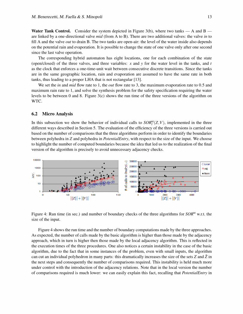
Figure 4: Run time (in sec.) and number of boundary checks of the three algorithms for SORM w.r.t. thesize of the input.

Figure 4 shows the run time and the number of boundary computations made by the three approaches.As expected, the number of calls made by the basic algorithm is higher than those made by the adjacencyapproach, which in turn is higher then those made by the local adjacency algorithm. This is reflected inthe execution times of the three procedures. One also notices a certain instability in the case of the basicalgorithm, due to the fact that in some instances of the problem, even with small inputs, the algorithmcan cut an individual polyhedron in many parts: this dramatically increases the size of the sets Z and Z inthe next steps and consequently the number of comparisons required. This instability is held much moreunder control with the introduction of the adjacency relations. Note that in the local version the numberof comparisons required is much lower: we can easily explain this fact, recalling that PotentialEntry in

14 Towards Efficient Exact Synthesis for Linear Hybrid Systems

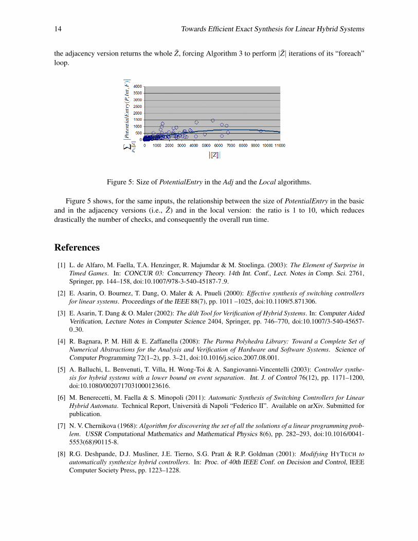
the adjacency version returns the whole Z, forcing Algorithm 3 to perform |Z| iterations of its “foreach”loop.

Figure 5: Size of PotentialEntry in the Adj and the Local algorithms.

Figure 5 shows, for the same inputs, the relationship between the size of PotentialEntry in the basicand in the adjacency versions (i.e., Z) and in the local version: the ratio is 1 to 10, which reducesdrastically the number of checks, and consequently the overall run time.

References

[1] L. de Alfaro, M. Faella, T.A. Henzinger, R. Majumdar & M. Stoelinga. (2003): The Element of Surprise inTimed Games. In: CONCUR 03: Concurrency Theory. 14th Int. Conf., Lect. Notes in Comp. Sci. 2761,Springer, pp. 144–158, doi:10.1007/978-3-540-45187-7 9.

[2] E. Asarin, O. Bournez, T. Dang, O. Maler & A. Pnueli (2000): Effective synthesis of switching controllersfor linear systems. Proceedings of the IEEE 88(7), pp. 1011 –1025, doi:10.1109/5.871306.

[3] E. Asarin, T. Dang & O. Maler (2002): The d/dt Tool for Verification of Hybrid Systems. In: Computer AidedVerification, Lecture Notes in Computer Science 2404, Springer, pp. 746–770, doi:10.1007/3-540-45657-0 30.

[4] R. Bagnara, P. M. Hill & E. Zaffanella (2008): The Parma Polyhedra Library: Toward a Complete Set ofNumerical Abstractions for the Analysis and Verification of Hardware and Software Systems. Science ofComputer Programming 72(1–2), pp. 3–21, doi:10.1016/j.scico.2007.08.001.

[5] A. Balluchi, L. Benvenuti, T. Villa, H. Wong-Toi & A. Sangiovanni-Vincentelli (2003): Controller synthe-sis for hybrid systems with a lower bound on event separation. Int. J. of Control 76(12), pp. 1171–1200,doi:10.1080/0020717031000123616.

[6] M. Benerecetti, M. Faella & S. Minopoli (2011): Automatic Synthesis of Switching Controllers for LinearHybrid Automata. Technical Report, Universita di Napoli “Federico II”. Available on arXiv. Submitted forpublication.

[7] N. V. Chernikova (1968): Algorithm for discovering the set of all the solutions of a linear programming prob-lem. USSR Computational Mathematics and Mathematical Physics 8(6), pp. 282–293, doi:10.1016/0041-5553(68)90115-8.

[8] R.G. Deshpande, D.J. Musliner, J.E. Tierno, S.G. Pratt & R.P. Goldman (2001): Modifying HYTECH toautomatically synthesize hybrid controllers. In: Proc. of 40th IEEE Conf. on Decision and Control, IEEEComputer Society Press, pp. 1223–1228.

M. Benerecetti, M. Faella & S. Minopoli 15

[9] G. Frehse (2005): PHAVer: Algorithmic Verification of Hybrid Systems Past HyTech. In: Proc. of HybridSystems: Computation and Control (HSCC), 8th International Workshop, Lect. Notes in Comp. Sci. 3414,Springer, pp. 258–273, doi:10.1007/978-3-540-31954-2 17.

[10] N. Halbwachs, Y.-E. Proy & P. Roumanoff (1997): Verification of Real-Time Systems using Linear RelationAnalysis. Formal Methods in System Design 11, pp. 157–185, doi:10.1023/A:1008678014487.

[11] T.A. Henzinger (1996): The Theory of Hybrid Automata. In: Proc. 11th IEEE Symp. Logic in Comp. Sci.,pp. 278–292, doi:0.1109/LICS.1996.561342.

[12] T.A. Henzinger, P.-H. Ho & H. Wong-Toi (1997): HyTech: A Model Checker for Hybrid Systems. SoftwareTools for Tech. Transfer 1, pp. 110–122, doi:10.1007/s100090050008.

[13] T.A. Henzinger, B. Horowitz & R. Majumdar (1999): Rectangular Hybrid Games. In: CONCUR 99: Con-currency Theory. 10th Int. Conf., Lect. Notes in Comp. Sci. 1664, Springer, pp. 320–335, doi:10.1007/3-540-48320-9 23.

[14] T.A. Henzinger, P.W. Kopke, A. Puri & P. Varaiya (1998): What’s Decidable about Hybrid Automata? J. ofComputer and System Sciences 57(1), pp. 94 – 124, doi:10.1006/jcss.1998.1581.

[15] O. Maler (2002): Control from computer science. Annual Reviews in Control 26(2), pp. 175–187,doi:10.1016/S1367-5788(02)00030-5.

[16] O. Maler, A. Pnueli & J. Sifakis (1995): On the Synthesis of Discrete Controllers for Timed Systems. In: Proc.of 12th Annual Symp. on Theor. Asp. of Comp. Sci., Lect. Notes in Comp. Sci. 900, Springer, doi:10.1007/3-540-59042-0 76.

[17] P.J. Ramadge & W.M. Wonham (1987): Supervisory Control of a Class of Discrete-Event Processes. SIAMJournal of Control and Optimization 25, pp. 206–230, doi:10.1137/0325013.

[18] C.J. Tomlin, J. Lygeros & S. Shankar Sastry (2000): A game theoretic approach to controller design forhybrid systems. Proc. of the IEEE 88(7), pp. 949–970.

[19] H. Le Verge (1992): A note on Chernikova’s Algorithm. Technical Report 635, IRISA, Rennes.[20] H. Wong-Toi (1997): The synthesis of controllers for linear hybrid automata. In: Proc. of the 36th

IEEE Conf. on Decision and Control, IEEE Computer Society Press, San Diego, CA, pp. 4607 – 4612,doi:10.1109/CDC.1997.649708.