Towards Exascale Simulations for Regional Earthquake Hazard and Risk

David McCallenLawrence Berkeley Laboratory& University of California Office

of the President

PEER Annual Meeting, January 18-19, 2018

The U.S. DOE has supported tremendous advancements in scientific HPC

100,000,000 (108) Flops

1,000,000,000,000,000,000 (1018) Flops

2020

Mainframe Era Vector Era Distributed Era

End of UndergroundNuclear Testing (UGT)

CORI Berkeley Lab30 Petaflop

TRINITY Los Alamos Lab40 Petaflop

SIERRA Livermore Lab125 Petaflop

100,000,000,000,000,000 (1017) Flops

The current (November 2017) top ten –the U.S. is no longer in a dominate role

The DOE Exascale (1018 Flops) Computing Project is a bold effort to accelerate the U.S.

Advanced hardware developmentApplication development

Software technology development

We were selected to develop an Exascaleapplication for earthquake hazard and risk

NEVADA & ESSI – finite deformation, inelasticFinite element codes for structures and soils

Eart

hqua

ke H

azar

dEa

rthq

uake

Ris

k

SW4 – 4th order finite difference geophysics code for wave propagation

A multidisciplinary team is essential – a National Laboratory scale problem

Dr. Anders Petersson Dr. Hans Johansen

Computational Science / Math

Dr. Artie RodgersSeismology

Dr. Arben Pitarka

Dr. Mamun Miah

Structural Engineering

Dr. Florina Petrone

Geotechnical EngineeringDr. Boris Jeremic

We propose to simulate to frequencies of engineering relevance – big challenge!

Pipelines Long-span Bridges Tall Buildings Low-rise Buildingsand Industrial Facilities

Energy SystemComponents

0.1 Hz 0.2 Hz 3.0 Hz 10.0 Hz

Nuclear PowerEquipment

25.0 Hz1.0 Hz 2.0 Hz

Frequency resolution of ground motions simulations as limited by

geologic/geotechnical materialmodels

Frequency resolution of ground motion simulations as limited by compute capabilities

0. Hz

Larger, faster forwardsimulations

Advanced geologiccharacterization

Seismologist

Exascale objective

Doubling the frequency resolution = 16X computational effort!

Today Exascale Future

Larger domain

Higher frequencyresolution

0-2 Hz motion 0-10 Hz motion

Simulation timesthat allow many

realizations

12+ hrs 3-4 hrs?

At the core is a transformation in ground motion simulation capability

Computational challenges to achieving the desired end-state

Run much bigger models much faster• Very large models at higher frequency

• Many realizations to account for uncertainties (e.g. fault rupture)

Representation of fine-scale geology• Waveform data inversion

• Stochastic geology

−122˚30' −122˚00' −121˚30' −121˚00'

36˚30'

37˚00'

37˚30'

38˚00'

25 km

8024−SJW

8019−WDS 8023−CLR

0 1000 2000 3000 4000 5000

S−Wave Speed, m/s

−40000

−30000

−20000

−10000

0

Depth(m)

0 20000 40000 60000 80000

Easting(m)

0 1 2 3 4 5

Vs(km/s)

−40000

−30000

−20000

−10000

0

Depth(m)

0 20000 40000 60000 80000

Easting(m)

0.00.51.01.52.02.53.03.54.04.55.05.5

Vs(km/s)Base geology from data Base + stochastic geology

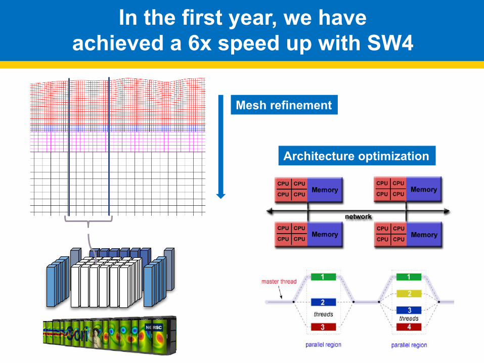
In the first year, we have achieved a 6x speed up with SW4

Mesh refinement

Architecture optimization

We have completed workflow for couplinggeophysics and engineering simulations

…

~ 2000 nonlinear building response history simulations

Distribution of buildingpeak interstory driftSurface motions from

regional geophysics simulation

Rupture hypocenter

0.5% 1.0% 2.5%

Elastic Behavior

LimitedPermanentDistortion

ModeratePermanentDistortion

LargePermanentDistortion

Earthquake hazard Earthquake risk

SW4

NEVADA

2048nodes

50nodes

Operational approach

T1 = 5.49 sec

T1 = 2.70 sec

T1 = 2.08 sec

T1 = 0.92 sec

Select infrastructurerepresentation

(e.g. nonlinear FEM)

Simulate Earthquake Scenario

Select InfrastructureRepresentation

Simulate EarthquakeRisk

…

Thousands ofground motions

Thousands ofresponse outputs

(e.g. peak interstory drift)

(a) (b)

(c) (d)

(e) 3-story FN M=7.0 (f) 40-story FN M=7.0

(g) 3-story FP M=7.0 (h) 40-story FP M=7.0

(c) 3-story FP M=6.5 (d) 40-story FP M=6.5

(a) 3-story FN M=6.5 (b) 40-story FN M=6.5

(a) (b)

(c) (d)

(e) 3-story FN M=7.0 (f) 40-story FN M=7.0

(g) 3-story FP M=7.0 (h) 40-story FP M=7.0

(c) 3-story FP M=6.5 (d) 40-story FP M=6.5

(a) 3-story FN M=6.5 (b) 40-story FN M=6.5

…

We have completed our first regional scale demonstrations of both hazard and risk

85 billion zones – Hayward Fault rupture simulation for 0 – 4 Hz

M=7 Hayward Fault event

We have completed our first regional scale demonstrations of both hazard and risk

Building Peak Interstory Drift Ratios

0.5% 1.0% 2.5%

Elastic Behavior

LimitedPermanentDistortion

ModeratePermanentDistortion

LargePermanentDistortionDOE standard

1020 limit states

We are critically assessing the realism of our results along the way

Do groundmotion

simulations “agree with”

observations?

Do structuralresponse

simulations “agree with”

observations?

We are evaluating the characteristics of the synthetic ground motions

S1 S2 S3

S1 S2 S3

M6.5

M7.0

We are seeing some interesting things

We are seeing some interesting things –drifts with real and synthetic records

Syntheticrecord

Realrecord

(Landers)

Building demands can be very localized

Peak Interstory drift Peak Interstory drift

Sites 2 Km apart

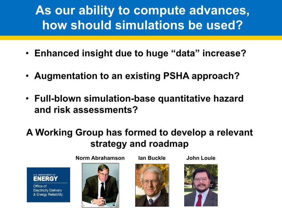
• Enhanced insight due to huge “data” increase?

• Augmentation to an existing PSHA approach?

• Full-blown simulation-base quantitative hazard and risk assessments?

A Working Group has formed to develop a relevant strategy and roadmap

As our ability to compute advances, how should simulations be used?

Norm Abrahamson Ian Buckle John Louie