HAL Id: inria-00370168https://hal.inria.fr/inria-00370168v1

Submitted on 23 Mar 2009 (v1), last revised 26 Apr 2009 (v3)

HAL is a multi-disciplinary open accessarchive for the deposit and dissemination of sci-entific research documents, whether they are pub-lished or not. The documents may come fromteaching and research institutions in France orabroad, or from public or private research centers.

L’archive ouverte pluridisciplinaire HAL, estdestinée au dépôt et à la diffusion de documentsscientifiques de niveau recherche, publiés ou non,émanant des établissements d’enseignement et derecherche français ou étrangers, des laboratoirespublics ou privés.

Towards New Technical Indicators for Trading Systemsand Risk Management

Michel Fliess, Cédric Join

To cite this version:Michel Fliess, Cédric Join. Towards New Technical Indicators for Trading Systems and Risk Manage-ment. 15th IFAC Symposium on System Identification (SYSID 2009), Jul 2009, Saint-Malo, France.2009. <inria-00370168v1>

Towards New Technical Indicators for

Trading Systems and Risk Management

Michel FLIESS ∗ Cédric JOIN ∗∗

∗ INRIA-ALIEN & LIX (CNRS, UMR 7161)École polytechnique, 91128 Palaiseau, France

Michel.Fliess@polytechnique.edu∗∗ INRIA-ALIEN & CRAN (CNRS, UMR 7039)

Nancy-Université, BP 239, 54506 Vandœuvre-lès-Nancy, FranceCedric.Join@cran.uhp-nancy.fr

Abstract. We derive two new technical indicators for trading systems and risk management.They stem from trends in time series, the existence of which has been recently mathematicallydemonstrated by the same authors (A mathematical proof of the existence of trends in financialtime series, Proc. Int. Conf. Systems Theory: Modelling, Analysis and Control, Fes, 2009), andfrom higher order quantities which replace the familiar statistical tools. Recent fast estimationtechniques of algebraic flavor are utilized. The first indicator tells us if the future price willbe above or below the forecasted trendline. The second one predicts abrupt changes. Severalpromising numerical experiments are detailed and commented.

1. INTRODUCTION

1.1 Generalities

This communication provides two new efficient technicalindicators for trading systems and risk management, bytaking advantage of the trends in financial time series.Remember that a precise mathematical definition of trendsas well as a proof of their existence have only been recentlygiven (Fliess & Join [2009a]). It confirms thus the most ba-sic assumption of technical analysis, which plays a key rôleamong many traders and financial professionals (see, e.g.,(Aronson [2007], Béchu, Bertrand & Nebenzahl [2008],Bollinger [2002], Kaufman [2005], Kirkpatrick & Dahlquist[2006], Lo & Hasanhodzic [2009], Murphy [1999]) and thereferences therein).

1.2 Brief description of our new indicators and of theirproperties

The definition and the existence of trends in (Fliess &Join [2009a]) is deduced from the Cartier-Perrin additivedecomposition (Cartier & Perrin [1995]) of a given timeseries f(t), which reads under a very weak integrabilitycondition:

f(t) = ftrend(t) + ffluctuation(t) (1)

ftrend(t) and ffluctuation(t) are respectively the trend anda “quickly fluctuating” function around 0. Introduce nowthe time series

ABS-DIFFι(t) = |ftrend(t + ι) − f(t)| (2)

where

• ι ≥ 0,

• ftrend(t+ ι) is the forecasted value of ftrend(t) at timet + ι, which is obtained as in (Fliess & Join [2009a]).

The trend ABS-DIFFι,trend(t) of ABS-DIFFι(t) is called ahigher-order trend associated to the time series f(t). Con-

struct now the quantities, which are vaguely reminiscentof the classic statistical skewness,

SKEWι(t) =

(

ftrend(t + ι) − f(t)

ABS-DIFFι,trend(t + ι)

)3

(3)

where ABS-DIFFι,trend(t + ι) is the forecasted value ofABS-DIFFι,trend(t) at time t + ι. Our two indicators arederived from Equations (2) and (3):

(1) The first one yields buy and sell signals by tellingif future prices will be above or below the forecastedtrendline. It greatly improves previous calculations in(Fliess & Join [2008b, 2009a]).

(2) The second one is related to risk management, which• is a central theme in modern quantitative finance,• seems to be more or less ignored until now in

the existing research literature related to tech-nical analysis (see, however, Dacorogna, Gençay,Müller, Olsen & Pictet [2001]).

The kind of volatility which is associated to Equa-tion (2) is exploited, via new algebraic techniquesstemming from (Fliess, Join & Mboup [2010]), inorder to forecast abrupt changes in the FOREX. Ourpromising computer simulations indicate a possiblealternative• not only to

· Monte Carlo techniques (see, e.g., (Glasser-man [2004]) and the references therein),

· the well known Value at Risk, or VaR,and its multiple variants (see, e.g., (Jorion[2001]) and the references therein),

• but also to more mathematically oriented workssuch as (Bouchaud & Potters [1997-2000], Malev-ergne & Sornette [2006], Mandelbrot & Hudson[2004]).

All those attempts rely on the search for a “good”probabilistic modeling, which often goes beyond the

Gaussian paradigm, whereas the need of any proba-bilistic model is bypassed here (see also Section 5.2and (Fliess & Join [2009a])).

1.3 Organization of the paper

Section 2 aims at presenting in plain words the Cartier-Perrin theorem and its utilization. Numerical experimentsare provided in Sections 3 and 4 respectively on theposition with respect to the forecasted trendline and on theprediction of abrupt changes. Some concluding remarks arediscussed in Section 5.

2. TRENDS AND QUICK FLUCTUATIONS

We refer to (Fliess & Join [2009a]) and to (Lobry & Sari[2008]) for details on the Cartier-Perrin theorem (Cartier& Perrin [1995]), which is expressed in the frameworkof nonstandard analysis. We will be employing here avery imprecise language, which hopefully will give to non-experts an intuitive feeling of what it is all about.

The decomposition in Equation (1) holds if f(t) is inte-grable. Then,

• the trend ftrend(t) is integrable and almost every-where continuous;

• the quickly fluctuating function ffluctuation(t) is de-

fined by the fact that its integral∫ b

affluctuation(τ)dτ

over any finite interval [a, b] is infinitesimal, i.e., “verysmall”.

Those quick fluctuations are similar to corrupting additivenoises in engineering, and especially in signal processingand in automatic control. The practical calculation of thetrend in (Fliess & Join [2009a]) is therefore achieved viaestimation techniques which were developed elsewhere andfor other purposes (see (Fliess, Join & Sira-Ramírez [2008],Mboup, Join & Fliess [2009]) and the references therein). Itshould be emphasized that those techniques may be viewedas an extension of the familiar moving average methodswhich are central in technical analysis (see, e.g., Béchu,Bertrand & Nebenzahl [2008]).

3. ABOVE OR BELOW THE FORECASTEDTRENDLINE?

Figure 1 displays the daily stock prices of Arcelor-Mittalfrom 7 July 1997 until 27 October 2008. 1 We first es-timate and forecast the trend of the daily prices as in(Fliess & Join [2009a]), i.e., by applying the techniquesof (Fliess, Join & Sira-Ramírez [2008], Mboup, Join &Fliess [2009]). It yields ABS-DIFFι(t), ABS-DIFFι,trend(t),

ABS-DIFFι,trend(t + ι), and SKEWι(t), which were de-fined in Section 1.2. The last quantity tells us if the futureprice will be above or below the forecasted trendline, if we

assume that its sign is the same as the sign of ftrend(t+ι)−f(t + ι). The meaning of the symbols △ and ∇ is obvious.The forecast index ι is respectively 1, 5, and 10.

The fact that the results do not deteriorate when theprediction time interval increases might seem rather sur-prising at first sight. This is explained by a parallel increase1 Those data are borrowed from http://finance.yahoo.com/.

0 500 1000 1500 2000 2500 30000

20

40

60

80

100

120

Figure 1. Arcelor-Mittal daily stock prices

of the time interval for determining the trend, i.e., we arenot working with the same trends. Our forecasts, whichgive 75% of exact results, are quite good.

4. TOWARDS THE FORECASTING OF ABRUPTCHANGES

The black lines in Figures 14-(a) represents the exchangerates between US Dollars (USD) and Euros (EUR) during2000 days, until 27 October 2008. 2 Our attempt to fore-cast abrupt changes is based on the following “empirical”fact:

An abrupt change in the FOREX is preceded bythe detection of an abrupt change of the “volatility”around the trend.

This general principle is implemented as follows:We take here as a measure of volatility the quantityABS-DIFF0(t) defined by Equation (2), where ι = 0.The corresponding signal is very “noisy”, and thus dif-ficult to analyze. We therefore replace it by its in-tegral

∫

ABS-DIFF0(τ)dτ , where, according to (Fliess[2006]), the noise is attenuated. Our task boils downto the detection of abrupt changes in the derivative of∫

ABS-DIFF0(τ)dτ , which is achieved via

• extrapolation techniques which were already utilizedin Section 3 and in (Fliess & Join [2009a]),

• the methods developed in (Fliess, Join & Mboup[2010]).

Figure 14 depicts the evolution and the forecasting ofthe various quantities considered above. Let us clarify ourresults thanks to Figures 14-(g) and 14-(h):

• In Figure 14-(g) one change-point is detected 10 daysahead but another one is missed.

• When the detection threshold becomes lower, Figure14-(h) shows that both change-points are detectedagain 10 days ahead.

2 Those data are borrowed from the European Central Bank.

5. CONCLUSION

5.1 New indicators

The efficiency of our two indicators should of course beconfirmed by further numerical and experimental studies,where high frequency data ought to be considered for theFOREX. Our second indicator will be completed in a nearfuture in order to predict if the abrupt change will be asudden increase or reduction. Many more indicators mightobviously be derived along the same lines, i.e., by takingadvantage of well chosen higher order trends.

5.2 Probability and statistics

We already criticized in (Fliess & Join [2009a]) the use ofprobability theory in quantitative finance. It is indeed dif-ficult, if not impossible, to model the inherent uncertaintyof such complex social behaviors via precise probabilitylaws. 3 We go here one step further and replace the tradi-tional statistical tools by new quantities like those definedby Equations (2) and (3). It should open new ways forinvestigating time series in general, in a model-free setting(see already (Fliess & Join [2008b]) for a first draft, and(Fliess & Join [2008a, 2009b]) for model-free control).

0 500 1000 1500 2000 2500 30000

20

40

60

80

100

120

Samples

Figure 2. Prices (black,-), filtered signal (blue,.), 1 dayforecast (red, - -), price’s forecast higher than thepredicted trend (green △), price’s forecast lower thanthe predicted trend (blue ▽) (1 day)

REFERENCES

D. Aronson. Evidence-Based Technical Analysis. Wiley,2007.

T. Béchu, E. Bertrand, J. Nebenzahl. L’analyse technique(6e éd.). Economica, 2008.

J. Bollinger. Bollinger on Bollinger Bands. McGraw-Hill,2002.

3 The epistemological difficulties related to probability in pureand applied sciences are discussed by Jaynes [2003] (the authorsthank Prof. A. Richard for pointing out to them this excellentreference). See also (Mouchot [1996]) about economy in general and,in particular, about probability and statistics in econometrics.

400 450 500 550 600 650 700 750 8002

4

6

8

10

12

14

16

18

20

Samples

Figure 3. Zoom of Figure 2 (1 day)

400 450 500 550 600 650 700 750 8000

1

2

3

4

5

6

7

8

9

10

Figure 4. ABS-DIFF1 (black,-), filtered signal (blue,.), 1day forecast (red, - -) (1 day)

J.-P. Bouchaud, M. Potters. Théorie des risques financiers.Eyrolles, 1997. English translation: Theory of FinancialRisks. Cambridge University Press, 2000.

P. Cartier, Y. Perrin. Integration over finite sets. In F. &M. Diener, editors. Nonstandard Analysis in Practice,pages 195–204. Springer, 1995.

M.M. Dacorogna, R. Gençay, U. Müller, R.B. Olsen, O.V.Pictet. An Introduction to High Frequency Finance.Academic Press, 2001.

M. Fliess. Analyse non standard du bruit. C.R. Acad. Sci.Paris Ser. I, 342:797–802, 2006.

M. Fliess, C. Join. Commande sans modèle et commande àmodèle restreint. e-STA, 5 (n◦ 4):1–23, 2008a (availableat http://hal.inria.fr/inria-00288107/en/).

M. Fliess, C. Join. Time series technical analysisvia new fast estimation methods: a preliminarystudy in mathematical finance. Proc. 23rd

IAR Workshop Advanced Control Diagnosis(IAR-ACD08), Coventry, 2008b (available athttp://hal.inria.fr/inria-00338099/en/).

M. Fliess, C. Join. A mathematical proof ofthe existence of trends in financial time series.

400 450 500 550 600 650 700 750 800−50

−40

−30

−20

−10

0

10

20

30

40

50

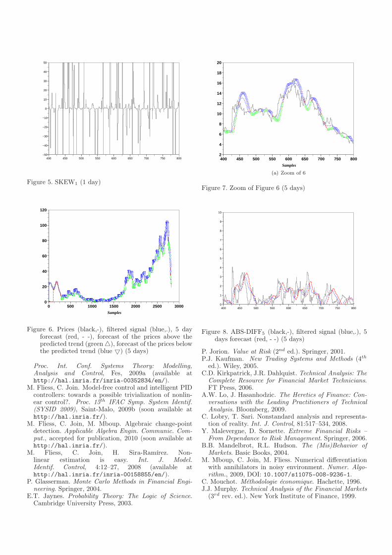
Figure 5. SKEW1 (1 day)

0 500 1000 1500 2000 2500 30000

20

40

60

80

100

120

Samples

Figure 6. Prices (black,-), filtered signal (blue,.), 5 dayforecast (red, - -), forecast of the prices above thepredicted trend (green △), forecast of the prices belowthe predicted trend (blue ▽) (5 days)

Proc. Int. Conf. Systems Theory: Modelling,Analysis and Control, Fes, 2009a (available athttp://hal.inria.fr/inria-00352834/en/).

M. Fliess, C. Join. Model-free control and intelligent PIDcontrollers: towards a possible trivialization of nonlin-ear control?. Proc. 15th IFAC Symp. System Identif.(SYSID 2009), Saint-Malo, 2009b (soon available athttp://hal.inria.fr/).

M. Fliess, C. Join, M. Mboup. Algebraic change-pointdetection. Applicable Algebra Engin. Communic. Com-put., accepted for publication, 2010 (soon available athttp://hal.inria.fr/).

M. Fliess, C. Join, H. Sira-Ramírez. Non-linear estimation is easy. Int. J. Model.Identif. Control, 4:12–27, 2008 (available athttp://hal.inria.fr/inria-00158855/en/).

P. Glasserman. Monte Carlo Methods in Financial Engi-neering. Springer, 2004.

E.T. Jaynes. Probability Theory: The Logic of Science.Cambridge University Press, 2003.

400 450 500 550 600 650 700 750 8002

4

6

8

10

12

14

16

18

20

Samples

(a) Zoom of 6

Figure 7. Zoom of Figure 6 (5 days)

400 450 500 550 600 650 700 750 8000

1

2

3

4

5

6

7

8

9

10

Figure 8. ABS-DIFF5 (black,-), filtered signal (blue,.), 5days forecast (red, - -) (5 days)

P. Jorion. Value at Risk (2nd ed.). Springer, 2001.P.J. Kaufman. New Trading Systems and Methods (4th

ed.). Wiley, 2005.C.D. Kirkpatrick, J.R. Dahlquist. Technical Analysis: The

Complete Resource for Financial Market Technicians.FT Press, 2006.

A.W. Lo, J. Hasanhodzic. The Heretics of Finance: Con-versations with the Leading Practitioners of TechnicalAnalysis. Bloomberg, 2009.

C. Lobry, T. Sari. Nonstandard analysis and representa-tion of reality. Int. J. Control, 81:517–534, 2008.

Y. Malevergne, D. Sornette. Extreme Financial Risks –From Dependance to Risk Management. Springer, 2006.

B.B. Mandelbrot, R.L. Hudson. The (Mis)Behavior ofMarkets. Basic Books, 2004.

M. Mboup, C. Join, M. Fliess. Numerical differentiationwith annihilators in noisy environment. Numer. Algo-rithm., 2009, DOI: 10.1007/s11075-008-9236-1.

C. Mouchot. Méthodologie économique. Hachette, 1996.J.J. Murphy. Technical Analysis of the Financial Markets

(3rd rev. ed.). New York Institute of Finance, 1999.

400 450 500 550 600 650 700 750 800−50

−40

−30

−20

−10

0

10

20

30

40

50

Figure 9. SKEW5 (5 days)

0 500 1000 1500 2000 2500 30000

20

40

60

80

100

120

Samples

Figure 10. Prices (black,-), filtered signal (blue,.), 10 day forecast(red, - -), price’s forecast higher than the predicted trend (green△), price’s forecast lower than the predicted trend (blue ▽) (10days)

400 450 500 550 600 650 700 750 8002

4

6

8

10

12

14

16

18

20

Samples

Figure 11. Zoom of Figure 10 (10 days)

400 450 500 550 600 650 700 750 8000

1

2

3

4

5

6

7

8

9

10

Figure 12. ABS-DIFF10 (black,-), filtered signal (blue,.),10 days forecast (red, - -) (10 days)

400 450 500 550 600 650 700 750 800−50

−40

−30

−20

−10

0

10

20

30

40

50

Figure 13. SKEW10 (10 days)

0 200 400 600 800 1000 1200 1400 1600 1800 20001.385

1.390

1.395

1.400

1.405

1.410

1.415

(a) Prices (black,-), filtered signal (blue,.), 10days forecast (red, - -)

0 200 400 600 800 1000 1200 1400 1600 1800 20000.0

0.5

1.0

1.5

2.0

2.5

3.0

(b)∫

ABS-DIFF0 (black,-) and 5 days fore-cast (red, - -)

0 200 400 600 800 1000 1200 1400 1600 1800 20000.000

0.001

0.002

0.003

0.004

0.005

0.006

0.007

0.008

(c)∫

ABS-DIFF0 (black,-), 10 days forecast(red, - -) and abrupt change location (red,+)

1460 1480 1500 1520 1540 1560 1580 1600 16200.000

0.001

0.002

0.003

0.004

0.005

0.006

0.007

0.008

(d) Zoom of Figure 14-(b)

0 200 400 600 800 1000 1200 1400 1600 1800 20000.000

0.001

0.002

0.003

0.004

0.005

0.006

0.007

0.008

(e)∫

ABS-DIFF0 (black,-), 10 days forecast(red, - -) and abrupt change location (red,+)

1460 1480 1500 1520 1540 1560 1580 1600 16200.000

0.001

0.002

0.003

0.004

0.005

0.006

0.007

0.008

(f) Zoom of Figure 14-(e)

0 200 400 600 800 1000 1200 1400 1600 1800 20001.385

1.39

1.395

1.4

1.405

1.41

1.415

non−detected

detected

(g) Prices (black,-) and abrupt change location (red,+)

0 200 400 600 800 1000 1200 1400 1600 1800 20001.385

1.39

1.395

1.4

1.405

1.41

1.415

detected

(h) Prices (black,-) and abrupt change location (red,+)

Figure 14. Daily exchange rate USD - EUR: 10 days forecasting