Towards Profit Maximization for Online SocialNetwork Providers

Jing TangSchool of Comp. Sci. & Eng.

Nanyang Technological UniversityEmail: tang0311@ntu.edu.sg

Xueyan TangSchool of Comp. Sci. & Eng.

Nanyang Technological UniversityEmail: asxytang@ntu.edu.sg

Junsong YuanSchool of EEE

Nanyang Technological UniversityEmail: jsyuan@ntu.edu.sg

Abstract—Online Social Networks (OSNs) attract billions ofusers to share information and communicate where viral mar-keting has emerged as a new way to promote the sales of products.An OSN provider is often hired by an advertiser to conduct viralmarketing campaigns. The OSN provider generates revenue fromthe commission paid by the advertiser which is determined bythe spread of its product information. Meanwhile, to propagateinfluence, the activities performed by users such as viewing videoads normally induce diffusion cost to the OSN provider. Inthis paper, we aim to find a seed set to optimize a new profitmetric that combines the benefit of influence spread with thecost of influence propagation for the OSN provider. Under manydiffusion models, our profit metric is the difference between twosubmodular functions which is challenging to optimize as it isneither submodular nor monotone. We design a general two-phase framework to select seeds for profit maximization anddevelop several bounds to measure the quality of the seed setconstructed. Experimental results with real OSN datasets showthat our approach can achieve high approximation guaranteesand significantly outperform the baseline algorithms, includingstate-of-the-art influence maximization algorithms.

I. INTRODUCTION

Information can be disseminated widely and rapidly throughOnline Social Networks (OSNs) (such as Facebook, Twitter,Flickr, Google+, and LinkedIn) with “word-of-mouth” effects.Viral marketing is a typical application that leverages OSNs asthe medium for information diffusion [9]. The market of OSNadvertisement is growing explosively. For example, Fortune[25] reports that the online and digital advertisement spendingfor the 2016 election of the United States will reach 1.2 billionUS dollars in which 49% is expected to go to social media.

Advertisers often delegate the operation of viral marketingcampaigns to OSN providers who have the complete infor-mation of their social network structures [3]. Providing viralmarketing services is a potential and promising approach thatOSN providers can explore for monetization. When hiring anOSN provider to conduct the viral marketing campaign, theadvertiser usually pays the OSN provider a commission foreach user that adopts its product or shares its ads. Thus, therevenue of the OSN provider generated from the commissionis determined by the spread of the product information.Meanwhile, to propagate influence, the activities performedby users such as viewing video ads normally induce diffusioncost to the OSN provider. For example, for a cloud-basedOSN running viral video marketing [20], the OSN will be

charged by the cloud for each video click due to the data trafficproduced. Intuitively, the number of clicks for each video isdependent on the number of connections among users that areactually used during the viral marketing campaign. Therefore,to maximize its profit, the OSN provider needs to accountfor both the reward of influence spread and the expense ofinfluence propagation, both of which are dependent on theseed users selected to initialize the viral marketing campaign.In this paper, we study the problem of finding a seed set tooptimize such a new profit metric that combines the benefit ofinfluence spread with the cost of influence propagation.

Our profit metric is challenging to optimize as it is signifi-cantly different from the influence metric that has been studiedwidely [6], [7], [12], [14], [15], [17], [22], [23], [24], [27],[28], [30], [32], [33], [34]. It is well known that the influencespread generated by a seed set is submodular and monotoneunder many diffusion models [1], [15], [26], which makes iteasy to design influence maximization algorithms with strongapproximation guarantees [21]. Some recent studies have ad-dressed profit maximization from the advertiser’s perspectiveby putting together the benefit of influence spread and the costof seed selection [19], [29], [31], [35]. In these studies, thecost of seed selection is modeled by the incentives (e.g., freesamples) provided to seed users. Since the seed selection costis given by the sum of the costs of individual seeds whichis modular, the resultant profit metric is still submodular. Incontrast, in our problem, both the revenue and cost of the OSNprovider are attached to the diffusion process. As a result,our profit metric can be viewed as the difference betweentwo submodular functions, which is neither submodular normonotone and is thus much more difficult to deal with.

In this paper, we propose a general two-phase frameworkto optimize profit for the OSN provider. Our framework iscomprised of a pruning phase that iteratively narrows down thesearch space and a search phase that uses heuristics to selectseed nodes within the reduced search space. We theoreticallyestablish the advantages of our pruning technique in improvingthe effectiveness and efficiency of any algorithm used in thesearch phase. We further derive several bounds on the maxi-mum achievable profit to evaluate the quality of the seed setsobtained by any algorithm. We conduct extensive experimentswith several real OSN datasets. The results demonstrate theeffectiveness and efficiency of our framework.

arX

iv:1

712.

0896

3v1

[cs

.SI]

24

Dec

201

7

The rest of this paper is organized as follows. Section IIreviews the related work. Section III defines the profit maxi-mization problem for the OSN provider. Section IV elaboratesthe design of our two-phase framework. Section V developsthe bounds for quality measurement. Section VI presents theexperimental evaluation. Finally, Section VII concludes thepaper.

II. RELATED WORK

Influence Maximization. Kempe et al. [15] formulated aninfluence maximization problem for a given seed set size withtwo basic diffusion models, namely the Independent Cascade(IC) and Linear Threshold (LT) models. They showed thatthe influence spreads under these models are submodularand monotone. Thus, they proposed a simple hill-climbinggreedy algorithm to address the problem, which can provide a(1−1/e)-approximation guarantee [21]. The follow-up studieshave mainly concentrated on improving the efficiency of thealgorithm implementation for large-scale OSNs [6], [7], [12],[14], [17], [22], [23], [24], [27], [28], [30], [32], [33], [34].Different from the above studies, we target at maximizing theprofit that accounts for both the benefit of influence spreadand the cost of influence propagation in viral marketing.

Profit Maximization. Maximizing the influence spreadalone has been shown to be ineffective for optimizing theprofit return of viral marketing [29], [31]. This is becausethe number of seeds selected yields a tradeoff between theexpense and reward of viral marketing. To avoid pre-settingthe number of seeds to select, some recent work studied profitmaximization from the advertiser’s perspective [19], [29],[31], [35]. These studies considered the cost of seed selectionwhich is modular and implies that their profit metric is stillsubmodular. They investigated heuristics to select seeds underthe assumption that the social network structures are availableto the advertiser. In practice, only the OSN providers havethe complete information of their social graphs and they oftenkeep the formation secret for business and privacy reasons[3], [16]. Therefore, the OSN providers are able to run viralmarketing campaigns more efficiently than the advertisers.Different from the above work, we formulate a new profitmaximization problem from the OSN provider’s perspectivethat takes into account the cost of information diffusion overthe social network. As shall be shown later, our profit metricis the difference between two submodular functions, which isneither submodular nor monotone.

Submodular Optimization. Iyer and Bilmes [13] inves-tigated optimizing the difference between two submodularfunctions. They showed that this problem is multiplicativelyinapproximable unless P=NP and proposed several heuristicmethods to address the problem. The greedy algorithm [15],[29] is another widely used heuristic for submodular optimiza-tion. We apply these heuristic methods to the search phase ofour two-phase framework. More importantly, we develop aniterative pruning technique to reduce the search space whichsignificantly improves these heuristics in terms of not onlyeffectiveness but also efficiency. In addition, we also derive

several upper bounds of the optimum to benchmark the outputof any algorithm.

III. PROBLEM FORMULATION

A. Preliminaries

Let G = (V,E) be a directed graph modeling an OSN,where the nodes V represent users and the edges E representthe connections among users (e.g., friendships on Facebook,followships on Twitter). For each directed edge 〈u, v〉 ∈ E,we refer to v as a neighbor of u, and refer to u as an inverseneighbor of v.

There are many diffusion models for the processes by whichinfluence propagates in social networks. The diffusion model isnormally a random process that starts with a set of seed nodesS. Initially, the seed nodes S are activated, while all the othernodes are not activated. When a node u becomes activated,it would attempt to further activate its neighbors which arenot yet activated. The diffusion process terminates when nomore node can be further activated. Let g ∼ G be a sampleoutcome of influence propagation by the diffusion process andlet Vg(S) be the set of nodes activated by the seed set S inthe sample outcome g. The influence spread of the seed set S,denoted by σ(S), is the expected number of nodes activatedover all possible sample outcomes of influence propagation,i.e., σ(S) = E[|Vg(S)|].B. The Profit Maximization Problem

As discussed, the influence spread is the benefit gained bythe OSN provider and the cost of influence propagation is theprice to pay for viral marketing. We assume that each node vin the social network is associated with a benefit weight b(v),which represents the benefit offered by activating v (e.g., thecommission received from the advertiser). The benefit β(S) ofinfluence spread generated by a seed set S is the total benefitbrought by all the nodes activated:

β(S) = E[ ∑v∈Vg(S)

b(v)]. (1)

To model the cost of influence propagation, we consider thediffusion process in the social network. Recall that when anode is activated, it attempts to further activate its neighborsthrough the connections to them in the social network. Withoutloss of generality, we assume that each node v is associatedwith a cost weight c(v), which represents the cost of infor-mation diffusion incurred by v in attempting to activate itsneighbors when it becomes activated (e.g., pushing video ads).The cost γ(S) of influence propagation introduced by a seedset S is the total cost incurred by all the nodes activated:

γ(S) = E[ ∑v∈Vg(S)

c(v)]. (2)

Then, we naturally define a profit metric from OSN provider’sperspective as the benefit of influence spread less the cost ofinfluence propagation, i.e., the profit φ(S) for running a viralmarketing campaign with a seed set S is given by

φ(S) = β(S)− γ(S), (3)

1

1

v1 v2

b=1.5,c=1

v3 v4

1 1

b=2,c=1

b=3,c=1 b=2,c=5

Vg(fg)=fg, Á (fg)=0

Vg(fv1g)=fv1,v2,v4g, Á (fv1g)=-1.5

Vg(fv3g)=fv3,v4g, Á (fv3g)=-1

Vg(fv1,v3g)=fv1,v2,v3,v4g, Á (fv1,v3g)=0.5

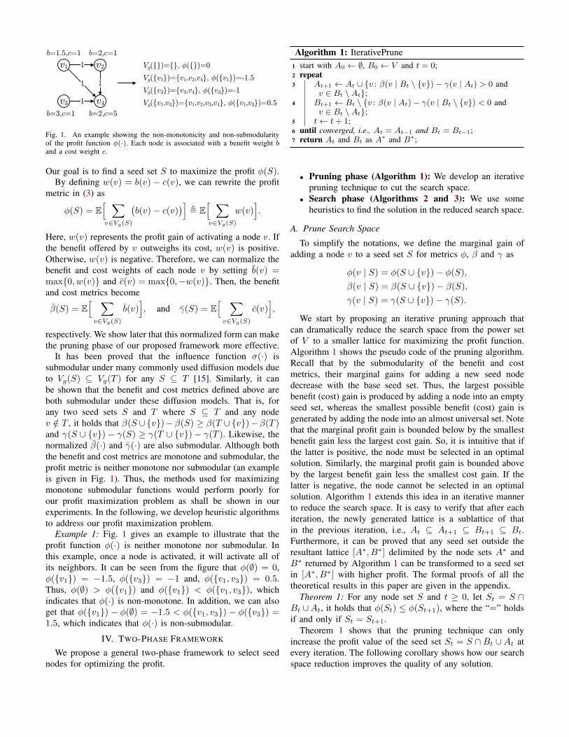
Fig. 1. An example showing the non-monotonicity and non-submodularityof the profit function φ(·). Each node is associated with a benefit weight band a cost weight c.

Our goal is to find a seed set S to maximize the profit φ(S).By defining w(v) = b(v) − c(v), we can rewrite the profit

metric in (3) as

φ(S) = E[ ∑v∈Vg(S)

(b(v)− c(v)

)], E

[ ∑v∈Vg(S)

w(v)].

Here, w(v) represents the profit gain of activating a node v. Ifthe benefit offered by v outweighs its cost, w(v) is positive.Otherwise, w(v) is negative. Therefore, we can normalize thebenefit and cost weights of each node v by setting b(v) =max{0, w(v)} and c(v) = max{0,−w(v)}. Then, the benefitand cost metrics become

β(S) = E[ ∑v∈Vg(S)

b(v)], and γ(S) = E

[ ∑v∈Vg(S)

c(v)],

respectively. We show later that this normalized form can makethe pruning phase of our proposed framework more effective.

It has been proved that the influence function σ(·) issubmodular under many commonly used diffusion models dueto Vg(S) ⊆ Vg(T ) for any S ⊆ T [15]. Similarly, it canbe shown that the benefit and cost metrics defined above areboth submodular under these diffusion models. That is, forany two seed sets S and T where S ⊆ T and any nodev /∈ T , it holds that β(S ∪{v})−β(S) ≥ β(T ∪{v})−β(T )and γ(S ∪ {v})− γ(S) ≥ γ(T ∪ {v})− γ(T ). Likewise, thenormalized β(·) and γ(·) are also submodular. Although boththe benefit and cost metrics are monotone and submodular, theprofit metric is neither monotone nor submodular (an exampleis given in Fig. 1). Thus, the methods used for maximizingmonotone submodular functions would perform poorly forour profit maximization problem as shall be shown in ourexperiments. In the following, we develop heuristic algorithmsto address our profit maximization problem.

Example 1: Fig. 1 gives an example to illustrate that theprofit function φ(·) is neither monotone nor submodular. Inthis example, once a node is activated, it will activate all ofits neighbors. It can be seen from the figure that φ(∅) = 0,φ({v1}) = −1.5, φ({v3}) = −1 and, φ({v1, v3}) = 0.5.Thus, φ(∅) > φ({v1}) and φ({v1}) < φ({v1, v3}), whichindicates that φ(·) is non-monotone. In addition, we can alsoget that φ({v1}) − φ(∅) = −1.5 < φ({v1, v3}) − φ({v3}) =1.5, which indicates that φ(·) is non-submodular.

IV. TWO-PHASE FRAMEWORK

We propose a general two-phase framework to select seednodes for optimizing the profit.

Algorithm 1: IterativePrune1 start with A0 ← ∅, B0 ← V and t = 0;2 repeat3 At+1 ← At ∪ {v : β(v | Bt \ {v})− γ(v | At) > 0 and

v ∈ Bt \At};4 Bt+1 ← Bt \ {v : β(v | At)− γ(v | Bt \ {v}) < 0 and

v ∈ Bt \At};5 t← t+ 1;6 until converged, i.e., At = At−1 and Bt = Bt−1;7 return At and Bt as A∗ and B∗;

• Pruning phase (Algorithm 1): We develop an iterativepruning technique to cut the search space.

• Search phase (Algorithms 2 and 3): We use someheuristics to find the solution in the reduced search space.

A. Prune Search Space

To simplify the notations, we define the marginal gain ofadding a node v to a seed set S for metrics φ, β and γ as

φ(v | S) = φ(S ∪ {v})− φ(S),

β(v | S) = β(S ∪ {v})− β(S),

γ(v | S) = γ(S ∪ {v})− γ(S).

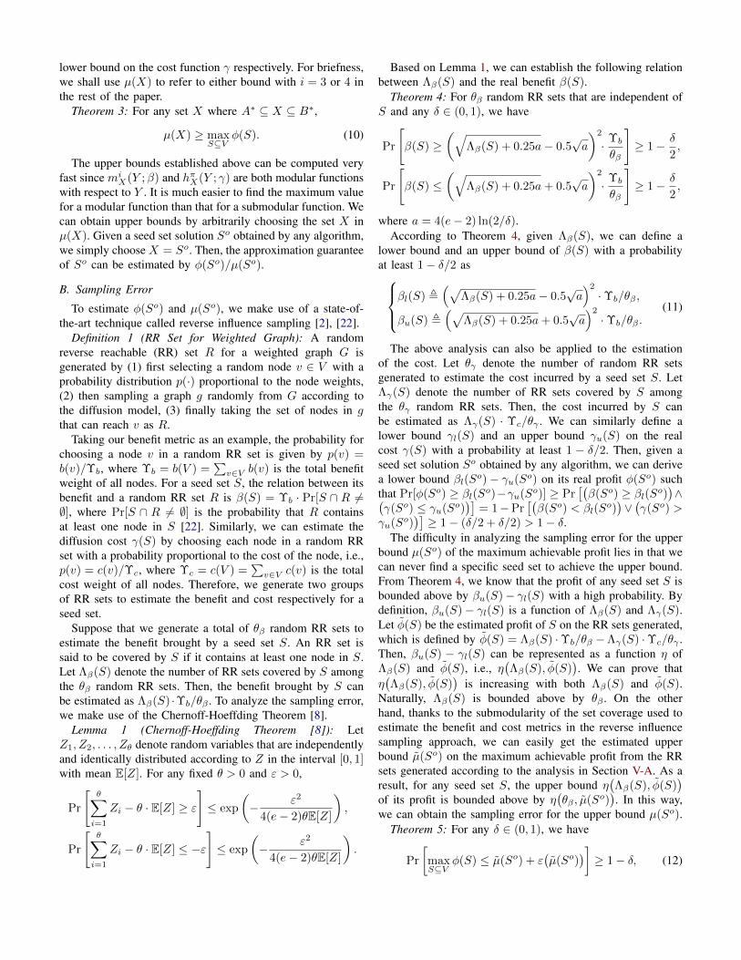
We start by proposing an iterative pruning approach thatcan dramatically reduce the search space from the power setof V to a smaller lattice for maximizing the profit function.Algorithm 1 shows the pseudo code of the pruning algorithm.Recall that by the submodularity of the benefit and costmetrics, their marginal gains for adding a new seed nodedecrease with the base seed set. Thus, the largest possiblebenefit (cost) gain is produced by adding a node into an emptyseed set, whereas the smallest possible benefit (cost) gain isgenerated by adding the node into an almost universal set. Notethat the marginal profit gain is bounded below by the smallestbenefit gain less the largest cost gain. So, it is intuitive that ifthe latter is positive, the node must be selected in an optimalsolution. Similarly, the marginal profit gain is bounded aboveby the largest benefit gain less the smallest cost gain. If thelatter is negative, the node cannot be selected in an optimalsolution. Algorithm 1 extends this idea in an iterative mannerto reduce the search space. It is easy to verify that after eachiteration, the newly generated lattice is a sublattice of thatin the previous iteration, i.e., At ⊆ At+1 ⊆ Bt+1 ⊆ Bt.Furthermore, it can be proved that any seed set outside theresultant lattice [A∗, B∗] delimited by the node sets A∗ andB∗ returned by Algorithm 1 can be transformed to a seed setin [A∗, B∗] with higher profit. The formal proofs of all thetheoretical results in this paper are given in the appendix.

Theorem 1: For any node set S and t ≥ 0, let St = S ∩Bt ∪At, it holds that φ(St) ≤ φ(St+1), where the “=” holdsif and only if St = St+1.

Theorem 1 shows that the pruning technique can onlyincrease the profit value of the seed set St = S ∩ Bt ∪ At atevery iteration. The following corollary shows how our searchspace reduction improves the quality of any solution.

0.3

0.3

v1 v2

b=1.5,c=1

v3 v4

0.4 0.2

b=2,c=1

b=3,c=1 b=2,c=5

Prune

Initialization: A0=fg, B0=fv1,v2,v3,v4gIteration 1: A1=fv3g, B1=fv1,v2,v3,v4gIteration 2: A2=fv3g, B2=fv1,v2,v3gIteration 3: A3=fv3g, B3=fv1,v2,v3gConverged, return A*=A3, B*=B3

Fig. 2. An example of iterative pruning under the Independent Cascadediffusion model. Each node is associated with a benefit weight b and a costweight c. Each edge has a propagation probability p.

Corollary 1: For any node set S, if S /∈ [A∗, B∗], thenφ(S) < φ(S ∩B∗ ∪A∗).

By Corollary 1, the pruning approach can always improvethe quality of any seed set S outside [A∗, B∗] by transformingit to the seed set S ∩ B∗ ∪ A∗ in [A∗, B∗]. Thus, the lattice[A∗, B∗] retains all the optimal seed sets. As a result, we canreduce the search space from the lattice [∅, V ] to [A∗, B∗].Our pruning approach can be used prior to any seed selectionalgorithms to improve the solution quality.

Corollary 2: For any seed set S∗ producing the maximumachievable profit, it holds that A∗ ⊆ S∗ ⊆ B∗.

Example 2: Fig. 2 gives an example to illustrate how thepruning algorithm works as well as the above theorem andcorollaries. This example assumes the Independent Cascade(IC) diffusion model. The IC model is a representative andmost widely-studied diffusion model for influence propagation[6], [7], [14], [15], [17], [22], [23], [24], [27], [28], [30], [32],[33], [34]. In the IC model, a propagation probability pu,v isassociated with each edge 〈u, v〉, representing the probabilityfor v to be activated by u through their connection. In thediffusion process, when a node u first becomes activated, ithas a chance to activate its neighbors who are not yet activated.Each such neighbor v would become activated with probabilitypu,v . This process repeats until no more node can be activated.For example, in Fig. 2, when {v1, v3} are selected as seeds, v2

would be activated with probability 0.3. Meanwhile, v4 wouldbe activated by v1 with probability 0.4, by v2 with probability0.3×0.2 = 0.06, and by v3 with probability 0.3. Thus, overall,v4 would be activated with probability 1 − (1 − 0.4) × (1 −0.06)× (1− 0.3) = 0.6052.

To conduct iterative pruning, A0 is initialized by ∅ andB0 is initialized by {v1, v2, v3, v4} respectively. To simplifythe notations, let φ−t (v) = β(v | Bt \ {v}) − γ(v | At)and φ+

t (v) = β(v | At) − γ(v | Bt \ {v}) describe thecalculations in Algorithm 1. At iteration 1, φ−1 (v1) = β(v1 |{v2, v3, v4}) − γ(v1 | ∅) = 1 × b(v1) −

(1 × c(v1) + 0.3 ×

c(v2)+(1− (1−0.4)× (1−0.3×0.2))× c(v4))

= 1.5− (1+0.3 + 2.18) = 1.5 − 3.48 = −1.98 < 0. Similarly, φ−1 (v2) =−0.6 < 0, φ−

1 (v3) = 0.5 > 0, φ−1 (v4) = −4.328 < 0,φ+

1 (v1) = 1.972 > 0, φ+1 (v2) = 1.7 > 0, φ+

1 (v3) = 2.6 > 0,and φ+

1 (v4) = 0.32 > 0. Thus, v3 is added to A1 sothat A1 = {v3} and B1 = {v1, v2, v3, v4}. At iteration 2,φ−2 (v1) = −1.326 < 0, φ−2 (v2) = −0.3 < 0, φ−2 (v4) =−2.828 < 0, φ+

2 (v1) = 1.7104 > 0, φ+2 (v2) = 1.58 > 0, and

φ+2 (v4) = −0.28 < 0. Thus, v4 is removed from B2 so that

A2 = {v3} and B2 = {v1, v2, v3}. At iteration 3, φ−3 (v1) =−0.878 < 0, φ−3 (v2) = −0.1824 < 0, φ+

3 (v1) = 0.5904 > 0,and φ+

3 (v2) = 1.286 > 0. Thus, both A3 and B3 remain thesame as in the previous iteration. As a result, A∗ = {v3} andB∗ = {v1, v2, v3} are returned. For a seed set S = {v2, v4} /∈[A∗, B∗], we have S1 = S ∩ B1 ∪ A1 = {v2, v3, v4} andS2 = S3 = S ∩B∗ ∪A∗ = {v2, v3}. Then, it can be obtainedthat φ(S) = −2 < φ(S1) = 0 < φ(S2) = 1.68, whichdemonstrates Theorem 1 and Corollary 1. Moreover, it is easyto verify that the optimal seed set S∗ = {v2, v3} belongs to[A∗, B∗], which confirms Corollary 2.

Finally, it can be shown that normalizing the benefit andcost weights as described in Section III-B can only increasethe amount of the search space cut by our pruning technique.

Theorem 2: Let A∗ and B∗ be the node sets returned byAlgorithm 1 under the normalized form. Then, A∗ ⊆ A∗ ⊆B∗ ⊆ B∗.

We shall experimentally evaluate the additional reduction inthe search space due to normalization in Section VI.

B. Heuristic Algorithms

We now present some heuristic methods to address the profitmaximization problem since there does not exist any polyno-mial time algorithm with any polynomial time multiplicativeapproximation guarantees unless P=NP [13].

Greedy Algorithm: We apply a simple hill-climbing ideato optimize the profit function (3). Algorithm 2 describes thepseudo code. In each iteration, the greedy heuristic adds a newnode u to S that has the largest marginal profit gain φ(u | S)until all the remaining nodes have negative marginal gains.

Algorithm 2: Greedy1 initialize S ← A∗;2 while True do3 find u← argmaxv∈B∗\S {φ(v | S)};4 if φ(u | S) ≤ 0 then return S;5 S ← S ∪ {u};

Modular-Modular Algorithm: Iyer and Bilmes [13] intro-duced a modular-modular (ModMod) algorithm for optimizingthe difference between submodular functions. Since we justneed to search the lattice [A∗, B∗] after pruning, we adapt theModMod algorithm as shown in Algorithm 3. In line 4 of Al-gorithm 3, hπXt(Y ;β) is a modular lower bound of β(Y ) thatis tight at set Xt, i.e., hπXt(Y ;β) ≤ β(Y ) for any Y ⊆ V andhπXt(X

t;β) = β(Xt), while mXt(Xt; γ) is a modular upper

bound of γ(Y ) that is also tight at Xt, i.e., mXt(Y ; γ) ≥ γ(Y )for any Y ⊆ V and mXt(X

t; γ) = γ(Xt). Thus, thedifference hπXt(Y ;β) − mXt(Y ; γ) is a lower bound of theprofit function φ(Y ). The algorithm maximizes the lowerbound in each iteration. Since the lower bound is tight atY = Xt, it is guaranteed that φ(Xt+1) ≥ hπXt(X

t+1;β) −mXt(X

t+1; γ) ≥ hπXt(Xt;β) −mXt(X

t; γ) = φ(Xt). Thisindicates that Algorithm 3 always increases the profit valueat every iteration. Examples of the modular upper and lowerbounds will be given in Section V-A.

Algorithm 3: Modular-Modular (ModMod)1 initialize X0 ← A∗ and t← 0;2 repeat3 choose the permutations of A∗, Xt \A∗, B∗ \Xt and

concatenate them as π;4 Xt+1 ← argmaxA∗⊆Y⊆B∗ hπXt(Y ;β)−mXt(Y ; γ);5 t← t+ 1;6 until converged, i.e., Xt = Xt−1;7 return Xt;

C. Discussions

Time Complexity: Evaluating the profit metric involvesestimating the influence spread given a seed set. Any existinginfluence estimation methods, such as Monte-Carlo simulation[15], [17], [24] and reverse influence sampling [2], [22], [23],[32], [33], can be used. Suppose the time complexity forcomputing the marginal profit gain of adding/removing a nodeinto/from a seed set is O(M). For the iterative pruning process(Algorithm 1), the size of the node set Bt\At to check reducesby at least 1 in each iteration. Therefore, it takes at mostO((|V | + |V | − 1 + · · · + 1)M

)= O(|V |2M) time to find

A∗ and B∗. After the reduction of the search space, there arek1 = |B∗ \A∗| nodes to be further examined. For the Greedyalgorithm, it checks k1− i+1 nodes in the ith iteration. Thus,it takes at most O(k2

1M) time, which means the total timecomplexity of the Greedy algorithm is O

((|V |2+k2

1)M). Each

iteration of the ModMod algorithm has a time complexity ofO(k1M). Let k2 denote the total number of iterations usedfor the ModMod algorithm. Then, the total time complexityof the ModMod algorithm is O

((|V |2 + k1k2)M

).

Diffusion Models: Our analysis and algorithms are generalframeworks that can be adapted to any diffusion models whichare submodular, such as the Independent Cascade and LinearThreshold models, the triggering model [15], the continuous-time models [5], [10], and the topic-aware models [1], [4].

V. PERFORMANCE ANALYSIS

The challenges to evaluate the quality of the seed setconstructed for the profit maximization problem are two-fold. First, optimizing the difference between two submodularfunctions is multiplicative inapproximability unless P=NP.Thus, it is difficult to measure the gap between the seed setobtained and an optimal seed set. Second, the random pro-cesses of many diffusion models are analytically intractable.For example, computing the exact influence spread under theIC diffusion model is #P-hard [6]. Thus, the benefit broughtand the cost incurred by a seed set can only be estimated viasome sampling approaches [15], [2]. As a result, the samplingerror also affects the quality measurement of the seed set.

We propose techniques to analyze the aforementioned gapand sampling error, which enable us to evaluate the approxi-mation guarantee of the seed set obtained by any algorithm onany given instance of the profit maximization problem. Specifi-cally, let So be the seed set constructed for a problem instance.We develop an upper bound µ on the maximum achievable

profit for the problem instance to characterize the gap betweenthe real profit value φ(So) and the maximum achievable profit.Note that both φ(So) and µ are to be estimated by sampling.Let φ(So) and µ be their estimated values. We further studythe sampling errors to bound the difference between φ(So)and φ(So) and the difference between µ and µ. In this way,we can obtain an approximation guarantee of So using theestimated values φ(So) and µ.

A. Upper Bound of Maximum Achievable Profit

To derive our bounds on the maximum achievable profit, wefirst introduce two modular bounds for submodular functions.

Modular Upper Bounds: For any submodular set functionf(·), we have the following two modular upper bounds m1

X

and m2X that are tight at a given set X [13]:

m1X(Y ) , f(X)−

∑v∈X\Y

f(v | V \ {v}) +∑

v∈Y \X

f(v | X), (4)

m2X(Y ) , f(X)−

∑v∈X\Y

f(v | X \ {v}) +∑

v∈Y \X

f(v | ∅). (5)

In the previous section, we have reduced the search space sothat only the sets belonging to [A∗, B∗] need to be consideredfor profit maximization. As a result, for any A∗ ⊆ X,Y ⊆ B∗,the above two upper bounds can be improved to:

m3X(Y ) , f(X)−

∑v∈X\Y

f(v | B∗ \ {v}) +∑

v∈Y \X

f(v | X), (6)

m4X(Y ) , f(X)−

∑v∈X\Y

f(v | X \ {v}) +∑

v∈Y \X

f(v | A∗). (7)

It is easy to show that the bounds m3X(Y ) and m4

X(Y ) remaintight at X , i.e., m3

X(X) = m4X(X) = f(X), and they are

tighter than m1X(Y ) and m2

X(Y ) at other sets, i.e., m1X(Y ) ≥

m3X(Y ) ≥ f(Y ) and m2

X(Y ) ≥ m4X(Y ) ≥ f(Y ) for any

A∗ ⊆ Y ⊆ B∗.Modular Lower Bounds: For any submodular set function

f(·), a modular lower bound hX that is tight at a given set Xcan be obtained as follows [11]. Let π be any permutation ofV that places all the nodes in X before the nodes in V \X .Let Sπi = {π(1), π(2), · · · , π(i)} be a chain formed by thepermutation, where Sπ0 = ∅ and Sπ|X| = X . Define

hπX(π(i)) = f(Sπi )− f(Sπi−1). (8)

Then, hπX(Y ) =∑v∈Y h

πX(v) is a lower bound of f(Y ),

which is tight at X , i.e., hπX(Y ) ≤ f(Y ) for any Y ⊆ Vand hπX(X) = f(X). After the search space is reduced to[A∗, B∗], we restrict π to any permutation of V in the orderof A∗, X \A∗ and B∗ \X .

Upper Bounds on Maximum Achievable Profit: Based onthe above bounds, we can derive two series of upper boundson the maximum value of the profit function φ(·) as follows.For any set X where A∗ ⊆ X ⊆ B∗, we define

µi(X) , maxA∗⊆Y⊆B∗

miX(Y ;β)− hπX(Y ; γ), (9)

where miX(Y ;β) (i = 3, 4) denotes the modular upper bound

on the benefit function β and hπX(Y ; γ) denotes the modular

lower bound on the cost function γ respectively. For briefness,we shall use µ(X) to refer to either bound with i = 3 or 4 inthe rest of the paper.

Theorem 3: For any set X where A∗ ⊆ X ⊆ B∗,

µ(X) ≥ maxS⊆V

φ(S). (10)

The upper bounds established above can be computed veryfast since mi

X(Y ;β) and hπX(Y ; γ) are both modular functionswith respect to Y . It is much easier to find the maximum valuefor a modular function than that for a submodular function. Wecan obtain upper bounds by arbitrarily choosing the set X inµ(X). Given a seed set solution So obtained by any algorithm,we simply choose X = So. Then, the approximation guaranteeof So can be estimated by φ(So)/µ(So).

B. Sampling Error

To estimate φ(So) and µ(So), we make use of a state-of-the-art technique called reverse influence sampling [2], [22].

Definition 1 (RR Set for Weighted Graph): A randomreverse reachable (RR) set R for a weighted graph G isgenerated by (1) first selecting a random node v ∈ V with aprobability distribution p(·) proportional to the node weights,(2) then sampling a graph g randomly from G according tothe diffusion model, (3) finally taking the set of nodes in gthat can reach v as R.

Taking our benefit metric as an example, the probability forchoosing a node v in a random RR set is given by p(v) =b(v)/Υb, where Υb = b(V ) =

∑v∈V b(v) is the total benefit

weight of all nodes. For a seed set S, the relation between itsbenefit and a random RR set R is β(S) = Υb · Pr[S ∩ R 6=∅], where Pr[S ∩ R 6= ∅] is the probability that R containsat least one node in S [22]. Similarly, we can estimate thediffusion cost γ(S) by choosing each node in a random RRset with a probability proportional to the cost of the node, i.e.,p(v) = c(v)/Υc, where Υc = c(V ) =

∑v∈V c(v) is the total

cost weight of all nodes. Therefore, we generate two groupsof RR sets to estimate the benefit and cost respectively for aseed set.

Suppose that we generate a total of θβ random RR sets toestimate the benefit brought by a seed set S. An RR set issaid to be covered by S if it contains at least one node in S.Let Λβ(S) denote the number of RR sets covered by S amongthe θβ random RR sets. Then, the benefit brought by S canbe estimated as Λβ(S) ·Υb/θβ . To analyze the sampling error,we make use of the Chernoff-Hoeffding Theorem [8].

Lemma 1 (Chernoff-Hoeffding Theorem [8]): LetZ1, Z2, . . . , Zθ denote random variables that are independentlyand identically distributed according to Z in the interval [0, 1]with mean E[Z]. For any fixed θ > 0 and ε > 0,

Pr

[θ∑i=1

Zi − θ · E[Z] ≥ ε]≤ exp

(− ε2

4(e− 2)θE[Z]

),

Pr

[θ∑i=1

Zi − θ · E[Z] ≤ −ε]≤ exp

(− ε2

4(e− 2)θE[Z]

).

Based on Lemma 1, we can establish the following relationbetween Λβ(S) and the real benefit β(S).

Theorem 4: For θβ random RR sets that are independent ofS and any δ ∈ (0, 1), we have

Pr

[β(S) ≥

(√Λβ(S) + 0.25a− 0.5

√a

)2

· Υb

θβ

]≥ 1− δ

2,

Pr

[β(S) ≤

(√Λβ(S) + 0.25a+ 0.5

√a

)2

· Υb

θβ

]≥ 1− δ

2,

where a = 4(e− 2) ln(2/δ).According to Theorem 4, given Λβ(S), we can define a

lower bound and an upper bound of β(S) with a probabilityat least 1− δ/2 asβl(S) ,

(√Λβ(S) + 0.25a− 0.5

√a)2

·Υb/θβ ,

βu(S) ,(√

Λβ(S) + 0.25a+ 0.5√a)2

·Υb/θβ .(11)

The above analysis can also be applied to the estimationof the cost. Let θγ denote the number of random RR setsgenerated to estimate the cost incurred by a seed set S. LetΛγ(S) denote the number of RR sets covered by S amongthe θγ random RR sets. Then, the cost incurred by S canbe estimated as Λγ(S) · Υc/θγ . We can similarly define alower bound γl(S) and an upper bound γu(S) on the realcost γ(S) with a probability at least 1 − δ/2. Then, given aseed set solution So obtained by any algorithm, we can derivea lower bound βl(So)− γu(So) on its real profit φ(So) suchthat Pr[φ(So) ≥ βl(So)−γu(So)] ≥ Pr

[(β(So) ≥ βl(So)

)∧(

γ(So) ≤ γu(So))]

= 1−Pr[(β(So) < βl(S

o))∨(γ(So) >

γu(So))]≥ 1− (δ/2 + δ/2) > 1− δ.

The difficulty in analyzing the sampling error for the upperbound µ(So) of the maximum achievable profit lies in that wecan never find a specific seed set to achieve the upper bound.From Theorem 4, we know that the profit of any seed set S isbounded above by βu(S)− γl(S) with a high probability. Bydefinition, βu(S)− γl(S) is a function of Λβ(S) and Λγ(S).Let φ(S) be the estimated profit of S on the RR sets generated,which is defined by φ(S) = Λβ(S) ·Υb/θβ −Λγ(S) ·Υc/θγ .Then, βu(S) − γl(S) can be represented as a function η ofΛβ(S) and φ(S), i.e., η

(Λβ(S), φ(S)

). We can prove that

η(Λβ(S), φ(S)

)is increasing with both Λβ(S) and φ(S).

Naturally, Λβ(S) is bounded above by θβ . On the otherhand, thanks to the submodularity of the set coverage used toestimate the benefit and cost metrics in the reverse influencesampling approach, we can easily get the estimated upperbound µ(So) on the maximum achievable profit from the RRsets generated according to the analysis in Section V-A. As aresult, for any seed set S, the upper bound η

(Λβ(S), φ(S)

)of its profit is bounded above by η

(θβ , µ(So)

). In this way,

we can obtain the sampling error for the upper bound µ(So).Theorem 5: For any δ ∈ (0, 1), we have

Pr

[maxS⊆V

φ(S) ≤ µ(So) + ε(µ(So)

)]≥ 1− δ, (12)

where ε(µ(So)

)is the sampling error for µ(So) such

that ε(µ(So)

)= ργ

√a((ρβθβ − µ(So)

)/ργ + 0.25a

)+

0.5a(ρβ − ργ) + ρβ√a(θβ + 0.25a), and ρβ = Υb/θβ and

ργ = Υc/θγ .By Theorems 4 and 5, we have the approximation guarantee

thatφ(So)

maxS⊆V φ(S)≥ βl(S

o)− γu(So)

µ(So) + ε(µ(So)

) (13)

with a probability at least 1− 2δ.

C. Reduce Sampling Error via Normalization

As discussed in Section III-B, we can normalize the benefitand cost weights by b(v) and c(v) for every node v ∈ V .Intuitively, the normalization can avoid unnecessary sam-ples conducted by the weights

∑v∈V min{b(v), c(v)} for

the estimations of both the benefit and cost. Therefore, thenormalization can reduce the sampling error by increasing thenumber of useful samples.

Theorem 6: For any seed set S and a fixed number ofsamples, let εφ be the sampling error limit that can provide aprobability guarantee of 1− δ, i.e., Pr[−εφ ≤ φ(S)−φ(S) ≤εφ] ≥ 1− δ, and let εφ be the sampling error limit under thenormalized form. We have εφ ≤ εφ.

Theorem 6 indicates that the normalization can improve thesolution quality which shall be demonstrated in the experi-ments.

VI. EVALUATION

A. Experimental Setup

Datasets. We use several real social networks availableat [18] to evaluate our proposed techniques. Due to spacelimitations, we report here the results for two representativedatasets, Google+ (108K nodes, 14M edges), and LiveJournal(5M nodes, 69M edges).

Algorithms. Recall that the ModMod algorithm needs amodular lower bound of the benefit function β(·) and amodular upper bound of the cost function γ(·). In Section V-A,we have presented one such lower bound and two such upperbounds. We use ModMod-1 to refer to that using the upperbound m3

X(Y ) defined in Eq. (6) and use ModMod-2 to referto that using the upper bound m4

X(Y ) defined in Eq. (7). Wecompare our two-phase methods with the following baselines.• Random: It randomly selects k nodes. We run the algo-

rithm 10 times and take their average as the expectedprofit.

• HighDegree: It selects k nodes with the highest degrees.• BenefitMax: It makes use of the reverse influence sam-

pling technique to find the top-k influential nodes forinfluence/benefit maximization [2], [22], [23], [32], [33].

The above baselines are executed on the entire social networkswithout applying any pruning technique. To explore differentseed numbers, in each baseline, we iterate through k = |V |

2i fori = 0, 1, . . . , 10 (where |V | is the network size) and choosethe k value producing the largest profit.

Parameter Settings. By default, we use the IC diffusionmodel (as described in Example 2 of Section IV-A), a uniformbenefit distribution (where every node has a unit benefit tomodel the commission paid by the advertiser for each useractivated), and a degree-proportional cost distribution (wherethe cost of each node is set proportional to its out-degree toemulate the diffusion cost for each activated user to push theproduct advertisement to all of his neighbors). In the IC model,we set the propagation probability pu,v of each edge 〈u, v〉to the reciprocal of v’s in-degree (the number of v’s inverseneighbors) as widely adopted by other studies [6], [14], [22],[23], [32], [33].

By default, we normalize the benefit and cost weights asdescribed in Section III-B. We use a scale factor r to controlthe ratio between the total cost and total benefit of all nodes.A higher r implies a higher cost of influence propagationrelative to the benefit of influence spread. The default valueof r is set to 1. We have tested a wide range of r values andobserved similar performance trends. In executing our two-phase methods and the baseline BenefitMax algorithm, wevary the number of RR sets generated to study the impact ofbenefit and cost estimations. To evaluate the profits of the seedsets returned by different algorithms, we generate a group ofvalidation RR sets to keep the estimation errors within 1% witha high probability at least 1− 10−6 according to Theorem 4.

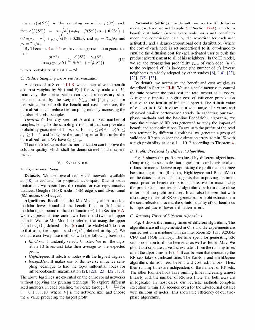
B. Profits Produced by Different Algorithms

Fig. 3 shows the profits produced by different algorithms.Comparing the seed selection algorithms, our heuristic algo-rithms are more effective in optimizing the profit than the threebaseline algorithms (Random, HighDegree and BenefitMax)on the datasets tested. This suggests that improving the influ-ence spread or benefit alone is not effective for maximizingthe profit. Our three heuristic algorithms perform quite closein terms of the profit produced. It can also be seen that withincreasing number of RR sets generated for profit estimation inthe seed selection process, the solution quality of our heuristicsis improved due to lower estimation errors.

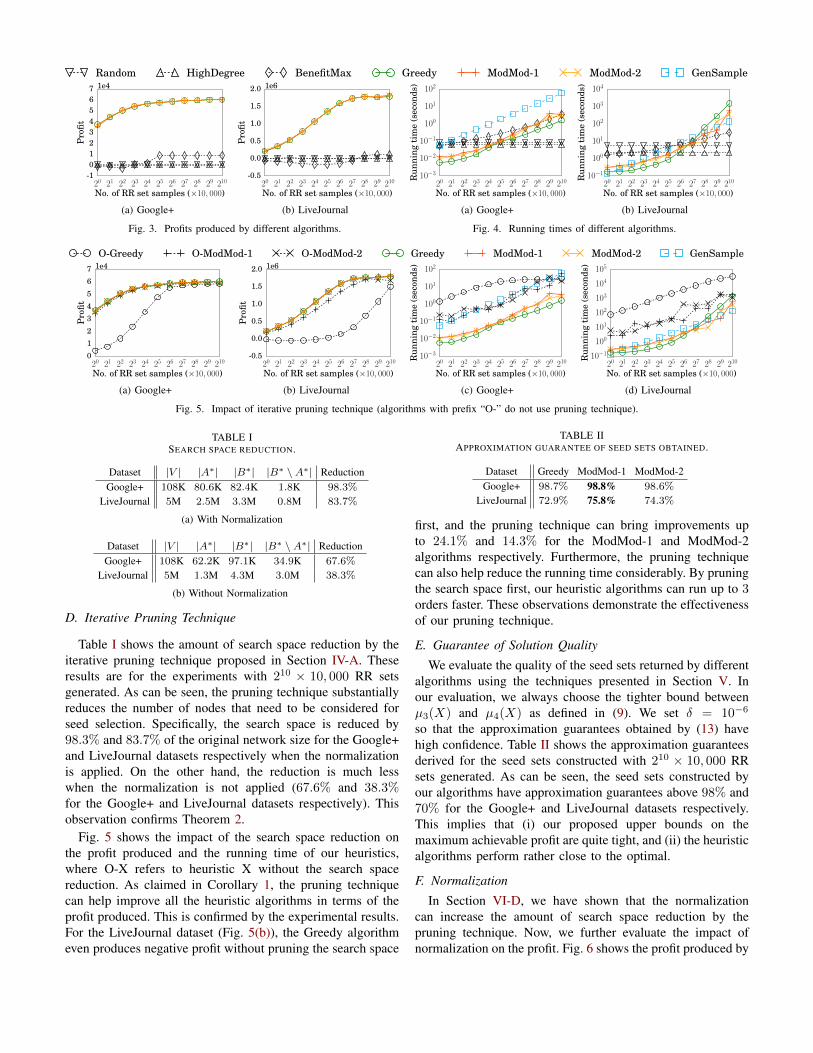
C. Running Times of Different Algorithms

Fig. 4 shows the running times of different algorithms. Thealgorithms are all implemented in C++ and the experiments arecarried out on a machine with an Intel Xeon E5-1650 3.2GHzCPU and 16GB memory. The time spent for generating RRsets is common to all our heuristics as well as BenefitMax. Weplot it as a separate curve and exclude it from the running timesof all the algorithms in Fig. 4. It can be seen that generating theRR sets takes significant time. The Random and HighDegreealgorithms do not need benefit and cost estimations. Thus,their running times are independent of the number of RR sets.The other four methods have running times increasing almostlinearly with the number of RR sets (note that both axes arein logscale). In most cases, our heuristic methods completeexecution within 100 seconds even for the LiveJournal datasetwith millions of nodes. This shows the efficiency of our two-phase algorithms.

Random HighDegree BenefitMax Greedy ModMod-1 ModMod-2 GenSample

20 21 22 23 24 25 26 27 28 29 210

No. of RR set samples (×10, 000)

-101234567

Pro

fit1e4

(a) Google+

20 21 22 23 24 25 26 27 28 29 210

No. of RR set samples (×10, 000)

-0.5

0.0

0.5

1.0

1.5

2.0

Pro

fit

1e6

(b) LiveJournal

Fig. 3. Profits produced by different algorithms.

20 21 22 23 24 25 26 27 28 29 210

No. of RR set samples (×10, 000)

10−3

10−2

10−1

100

101

102

Run

ning

tim

e(s

econ

ds)

(a) Google+

20 21 22 23 24 25 26 27 28 29 210

No. of RR set samples (×10, 000)

10−1

100

101

102

103

104

Run

ning

tim

e(s

econ

ds)

(b) LiveJournal

Fig. 4. Running times of different algorithms.

O-Greedy O-ModMod-1 O-ModMod-2 Greedy ModMod-1 ModMod-2 GenSample

20 21 22 23 24 25 26 27 28 29 210

No. of RR set samples (×10, 000)

01234567

Pro

fit

1e4

(a) Google+

20 21 22 23 24 25 26 27 28 29 210

No. of RR set samples (×10, 000)

-0.5

0.0

0.5

1.0

1.5

2.0

Pro

fit

1e6

(b) LiveJournal

20 21 22 23 24 25 26 27 28 29 210

No. of RR set samples (×10, 000)

10−3

10−2

10−1

100

101

102

Run

ning

tim

e(s

econ

ds)

(c) Google+

20 21 22 23 24 25 26 27 28 29 210

No. of RR set samples (×10, 000)

10−1

100

101

102

103

104

105

Run

ning

tim

e(s

econ

ds)

(d) LiveJournal

Fig. 5. Impact of iterative pruning technique (algorithms with prefix “O-” do not use pruning technique).

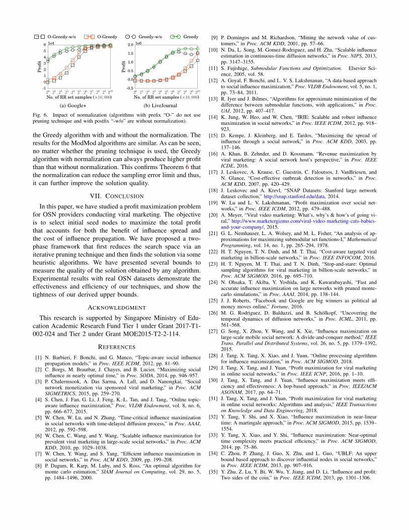
TABLE ISEARCH SPACE REDUCTION.

Dataset |V | |A∗| |B∗| |B∗ \A∗| ReductionGoogle+ 108K 80.6K 82.4K 1.8K 98.3%

LiveJournal 5M 2.5M 3.3M 0.8M 83.7%

(a) With Normalization

Dataset |V | |A∗| |B∗| |B∗ \A∗| ReductionGoogle+ 108K 62.2K 97.1K 34.9K 67.6%

LiveJournal 5M 1.3M 4.3M 3.0M 38.3%

(b) Without Normalization

D. Iterative Pruning Technique

Table I shows the amount of search space reduction by theiterative pruning technique proposed in Section IV-A. Theseresults are for the experiments with 210 × 10, 000 RR setsgenerated. As can be seen, the pruning technique substantiallyreduces the number of nodes that need to be considered forseed selection. Specifically, the search space is reduced by98.3% and 83.7% of the original network size for the Google+and LiveJournal datasets respectively when the normalizationis applied. On the other hand, the reduction is much lesswhen the normalization is not applied (67.6% and 38.3%for the Google+ and LiveJournal datasets respectively). Thisobservation confirms Theorem 2.

Fig. 5 shows the impact of the search space reduction onthe profit produced and the running time of our heuristics,where O-X refers to heuristic X without the search spacereduction. As claimed in Corollary 1, the pruning techniquecan help improve all the heuristic algorithms in terms of theprofit produced. This is confirmed by the experimental results.For the LiveJournal dataset (Fig. 5(b)), the Greedy algorithmeven produces negative profit without pruning the search space

TABLE IIAPPROXIMATION GUARANTEE OF SEED SETS OBTAINED.

Dataset Greedy ModMod-1 ModMod-2Google+ 98.7% 98.8% 98.6%

LiveJournal 72.9% 75.8% 74.3%

first, and the pruning technique can bring improvements upto 24.1% and 14.3% for the ModMod-1 and ModMod-2algorithms respectively. Furthermore, the pruning techniquecan also help reduce the running time considerably. By pruningthe search space first, our heuristic algorithms can run up to 3orders faster. These observations demonstrate the effectivenessof our pruning technique.

E. Guarantee of Solution Quality

We evaluate the quality of the seed sets returned by differentalgorithms using the techniques presented in Section V. Inour evaluation, we always choose the tighter bound betweenµ3(X) and µ4(X) as defined in (9). We set δ = 10−6

so that the approximation guarantees obtained by (13) havehigh confidence. Table II shows the approximation guaranteesderived for the seed sets constructed with 210 × 10, 000 RRsets generated. As can be seen, the seed sets constructed byour algorithms have approximation guarantees above 98% and70% for the Google+ and LiveJournal datasets respectively.This implies that (i) our proposed upper bounds on themaximum achievable profit are quite tight, and (ii) the heuristicalgorithms perform rather close to the optimal.

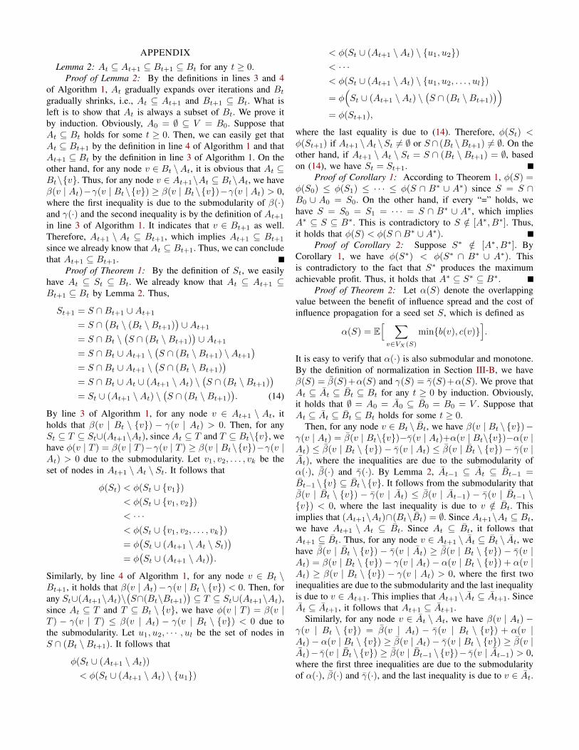
F. Normalization

In Section VI-D, we have shown that the normalizationcan increase the amount of search space reduction by thepruning technique. Now, we further evaluate the impact ofnormalization on the profit. Fig. 6 shows the profit produced by

O-Greedy-w/o O-Greedy Greedy-w/o Greedy

20 21 22 23 24 25 26 27 28 29 210

No. of RR set samples (×10, 000)

-10123456

Pro

fit1e4

(a) Google+

20 21 22 23 24 25 26 27 28 29 210

No. of RR set samples (×10, 000)

-0.5

0.0

0.5

1.0

1.5

2.0

Pro

fit

1e6

(b) LiveJournal

Fig. 6. Impact of normalization (algorithms with prefix “O-” do not usepruning technique and with postfix “-w/o” are without normalization).

the Greedy algorithm with and without the normalization. Theresults for the ModMod algorithms are similar. As can be seen,no matter whether the pruning technique is used, the Greedyalgorithm with normalization can always produce higher profitthan that without normalization. This confirms Theorem 6 thatthe normalization can reduce the sampling error limit and thus,it can further improve the solution quality.

VII. CONCLUSION

In this paper, we have studied a profit maximization problemfor OSN providers conducting viral marketing. The objectiveis to select initial seed nodes to maximize the total profitthat accounts for both the benefit of influence spread andthe cost of influence propagation. We have proposed a two-phase framework that first reduces the search space via aniterative pruning technique and then finds the solution via someheuristic algorithms. We have presented several bounds tomeasure the quality of the solution obtained by any algorithm.Experimental results with real OSN datasets demonstrate theeffectiveness and efficiency of our techniques, and show thetightness of our derived upper bounds.

ACKNOWLEDGMENT

This research is supported by Singapore Ministry of Edu-cation Academic Research Fund Tier 1 under Grant 2017-T1-002-024 and Tier 2 under Grant MOE2015-T2-2-114.

REFERENCES

[1] N. Barbieri, F. Bonchi, and G. Manco, “Topic-aware social influencepropagation models,” in Proc. IEEE ICDM, 2012, pp. 81–90.

[2] C. Borgs, M. Brautbar, J. Chayes, and B. Lucier, “Maximizing socialinfluence in nearly optimal time,” in Proc. SODA, 2014, pp. 946–957.

[3] P. Chalermsook, A. Das Sarma, A. Lall, and D. Nanongkai, “Socialnetwork monetization via sponsored viral marketing,” in Proc. ACMSIGMETRICS, 2015, pp. 259–270.

[4] S. Chen, J. Fan, G. Li, J. Feng, K.-L. Tan, and J. Tang, “Online topic-aware influence maximization,” Proc. VLDB Endowment, vol. 8, no. 6,pp. 666–677, 2015.

[5] W. Chen, W. Lu, and N. Zhang, “Time-critical influence maximizationin social networks with time-delayed diffusion process,” in Proc. AAAI,2012, pp. 592–598.

[6] W. Chen, C. Wang, and Y. Wang, “Scalable influence maximization forprevalent viral marketing in large-scale social networks,” in Proc. ACMKDD, 2010, pp. 1029–1038.

[7] W. Chen, Y. Wang, and S. Yang, “Efficient influence maximization insocial networks,” in Proc. ACM KDD, 2009, pp. 199–208.

[8] P. Dagum, R. Karp, M. Luby, and S. Ross, “An optimal algorithm formonte carlo estimation,” SIAM Journal on Computing, vol. 29, no. 5,pp. 1484–1496, 2000.

[9] P. Domingos and M. Richardson, “Mining the network value of cus-tomers,” in Proc. ACM KDD, 2001, pp. 57–66.

[10] N. Du, L. Song, M. Gomez-Rodriguez, and H. Zha, “Scalable influenceestimation in continuous-time diffusion networks,” in Proc. NIPS, 2013,pp. 3147–3155.

[11] S. Fujishige, Submodular Functions and Optimization. Elsevier Sci-ence, 2005, vol. 58.

[12] A. Goyal, F. Bonchi, and L. V. S. Lakshmanan, “A data-based approachto social influence maximization,” Proc. VLDB Endowment, vol. 5, no. 1,pp. 73–84, 2011.

[13] R. Iyer and J. Bilmes, “Algorithms for approximate minimization of thedifference between submodular functions, with applications,” in Proc.UAI, 2012, pp. 407–417.

[14] K. Jung, W. Heo, and W. Chen, “IRIE: Scalable and robust influencemaximization in social networks,” in Proc. IEEE ICDM, 2012, pp. 918–923.

[15] D. Kempe, J. Kleinberg, and E. Tardos, “Maximizing the spread ofinfluence through a social network,” in Proc. ACM KDD, 2003, pp.137–146.

[16] A. Khan, B. Zehnder, and D. Kossmann, “Revenue maximization byviral marketing: A social network host’s perspective,” in Proc. IEEEICDE, 2016.

[17] J. Leskovec, A. Krause, C. Guestrin, C. Faloutsos, J. VanBriesen, andN. Glance, “Cost-effective outbreak detection in networks,” in Proc.ACM KDD, 2007, pp. 420–429.

[18] J. Leskovec and A. Krevl, “SNAP Datasets: Stanford large networkdataset collection,” http://snap.stanford.edu/data, 2014.

[19] W. Lu and L. V. Lakshmanan, “Profit maximization over social net-works,” in Proc. IEEE ICDM, 2012, pp. 479–488.

[20] A. Meyer, “Viral video marketing: What’s, why’s & how’s of going vi-ral,” http://www.marketergizmo.com/viral-video-marketing-cats-babies-and-your-company/, 2015.

[21] G. L. Nemhauser, L. A. Wolsey, and M. L. Fisher, “An analysis of ap-proximations for maximizing submodular set functions-I,” MathematicalProgramming, vol. 14, no. 1, pp. 265–294, 1978.

[22] H. T. Nguyen, T. N. Dinh, and M. T. Thai, “Cost-aware targeted viralmarketing in billion-scale networks,” in Proc. IEEE INFOCOM, 2016.

[23] H. T. Nguyen, M. T. Thai, and T. N. Dinh, “Stop-and-stare: Optimalsampling algorithms for viral marketing in billion-scale networks,” inProc. ACM SIGMOD, 2016, pp. 695–710.

[24] N. Ohsaka, T. Akiba, Y. Yoshida, and K. Kawarabayashi, “Fast andaccurate influence maximization on large networks with pruned monte-carlo simulations,” in Proc. AAAI, 2014, pp. 138–144.

[25] J. J. Roberts, “Facebook and Google are big winners as political admoney moves online,” Fortune, 2016.

[26] M. G. Rodriguez, D. Balduzzi, and B. Scholkopf, “Uncovering thetemporal dynamics of diffusion networks,” in Proc. ICML, 2011, pp.561–568.

[27] G. Song, X. Zhou, Y. Wang, and K. Xie, “Influence maximization onlarge-scale mobile social network: A divide-and-conquer method,” IEEETrans. Parallel and Distributed Systems, vol. 26, no. 5, pp. 1379–1392,2015.

[28] J. Tang, X. Tang, X. Xiao, and J. Yuan, “Online processing algorithmsfor influence maximization,” in Proc. ACM SIGMOD, 2018.

[29] J. Tang, X. Tang, and J. Yuan, “Profit maximization for viral marketingin online social networks,” in Proc. IEEE ICNP, 2016, pp. 1–10.

[30] J. Tang, X. Tang, and J. Yuan, “Influence maximization meets effi-ciency and effectiveness: A hop-based approach,” in Proc. IEEE/ACMASONAM, 2017, pp. 64–71.

[31] J. Tang, X. Tang, and J. Yuan, “Profit maximization for viral marketingin online social networks: Algorithms and analysis,” IEEE Transactionson Knowledge and Data Engineering, 2018.

[32] Y. Tang, Y. Shi, and X. Xiao, “Influence maximization in near-lineartime: A martingale approach,” in Proc. ACM SIGMOD, 2015, pp. 1539–1554.

[33] Y. Tang, X. Xiao, and Y. Shi, “Influence maximization: Near-optimaltime complexity meets practical efficiency,” in Proc. ACM SIGMOD,2014, pp. 75–86.

[34] C. Zhou, P. Zhang, J. Guo, X. Zhu, and L. Guo, “UBLF: An upperbound based approach to discover influential nodes in social networks,”in Proc. IEEE ICDM, 2013, pp. 907–916.

[35] Y. Zhu, Z. Lu, Y. Bi, W. Wu, Y. Jiang, and D. Li, “Influence and profit:Two sides of the coin,” in Proc. IEEE ICDM, 2013, pp. 1301–1306.

APPENDIX

Lemma 2: At ⊆ At+1 ⊆ Bt+1 ⊆ Bt for any t ≥ 0.Proof of Lemma 2: By the definitions in lines 3 and 4

of Algorithm 1, At gradually expands over iterations and Btgradually shrinks, i.e., At ⊆ At+1 and Bt+1 ⊆ Bt. What isleft is to show that At is always a subset of Bt. We prove itby induction. Obviously, A0 = ∅ ⊆ V = B0. Suppose thatAt ⊆ Bt holds for some t ≥ 0. Then, we can easily get thatAt ⊆ Bt+1 by the definition in line 4 of Algorithm 1 and thatAt+1 ⊆ Bt by the definition in line 3 of Algorithm 1. On theother hand, for any node v ∈ Bt \At, it is obvious that At ⊆Bt\{v}. Thus, for any node v ∈ At+1\At ⊆ Bt\At, we haveβ(v | At)−γ(v | Bt \{v}) ≥ β(v | Bt \{v})−γ(v | At) > 0,where the first inequality is due to the submodularity of β(·)and γ(·) and the second inequality is by the definition of At+1

in line 3 of Algorithm 1. It indicates that v ∈ Bt+1 as well.Therefore, At+1 \ At ⊆ Bt+1, which implies At+1 ⊆ Bt+1

since we already know that At ⊆ Bt+1. Thus, we can concludethat At+1 ⊆ Bt+1.

Proof of Theorem 1: By the definition of St, we easilyhave At ⊆ St ⊆ Bt. We already know that At ⊆ At+1 ⊆Bt+1 ⊆ Bt by Lemma 2. Thus,

St+1 = S ∩Bt+1 ∪At+1

= S ∩(Bt \ (Bt \Bt+1)

)∪At+1

= S ∩Bt \(S ∩ (Bt \Bt+1)

)∪At+1

= S ∩Bt ∪At+1 \(S ∩ (Bt \Bt+1) \At+1

)= S ∩Bt ∪At+1 \

(S ∩ (Bt \Bt+1)

)= S ∩Bt ∪At ∪ (At+1 \At) \

(S ∩ (Bt \Bt+1)

)= St ∪ (At+1 \At) \

(S ∩ (Bt \Bt+1)

). (14)

By line 3 of Algorithm 1, for any node v ∈ At+1 \ At, itholds that β(v | Bt \ {v}) − γ(v | At) > 0. Then, for anySt ⊆ T ⊆ St∪(At+1\At), since At ⊆ T and T ⊆ Bt\{v}, wehave φ(v | T ) = β(v | T )−γ(v | T ) ≥ β(v | Bt\{v})−γ(v |At) > 0 due to the submodularity. Let v1, v2, . . . , vk be theset of nodes in At+1 \At \ St. It follows that

φ(St) < φ(St ∪ {v1})< φ(St ∪ {v1, v2})< · · ·< φ(St ∪ {v1, v2, . . . , vk})= φ

(St ∪ (At+1 \At \ St)

)= φ

(St ∪ (At+1 \At)

).

Similarly, by line 4 of Algorithm 1, for any node v ∈ Bt \Bt+1, it holds that β(v | At)− γ(v | Bt \ {v}) < 0. Then, forany St∪(At+1\At)\

(S∩(Bt\Bt+1)

)⊆ T ⊆ St∪(At+1\At),

since At ⊆ T and T ⊆ Bt \ {v}, we have φ(v | T ) = β(v |T ) − γ(v | T ) ≤ β(v | At) − γ(v | Bt \ {v}) < 0 due tothe submodularity. Let u1, u2, · · · , ul be the set of nodes inS ∩ (Bt \Bt+1). It follows that

φ(St ∪ (At+1 \At))< φ(St ∪ (At+1 \At) \ {u1})

< φ(St ∪ (At+1 \At) \ {u1, u2})< · · ·< φ(St ∪ (At+1 \At) \ {u1, u2, . . . , ul})= φ

(St ∪ (At+1 \At) \

(S ∩ (Bt \Bt+1)

))= φ(St+1),

where the last equality is due to (14). Therefore, φ(St) <φ(St+1) if At+1 \At \St 6= ∅ or S ∩ (Bt \Bt+1) 6= ∅. On theother hand, if At+1 \ At \ St = S ∩ (Bt \ Bt+1) = ∅, basedon (14), we have St = St+1.

Proof of Corollary 1: According to Theorem 1, φ(S) =φ(S0) ≤ φ(S1) ≤ · · · ≤ φ(S ∩ B∗ ∪ A∗) since S = S ∩B0 ∪ A0 = S0. On the other hand, if every “=” holds, wehave S = S0 = S1 = · · · = S ∩ B∗ ∪ A∗, which impliesA∗ ⊆ S ⊆ B∗. This is contradictory to S /∈ [A∗, B∗]. Thus,it holds that φ(S) < φ(S ∩B∗ ∪A∗).

Proof of Corollary 2: Suppose S∗ /∈ [A∗, B∗]. ByCorollary 1, we have φ(S∗) < φ(S∗ ∩ B∗ ∪ A∗). Thisis contradictory to the fact that S∗ produces the maximumachievable profit. Thus, it holds that A∗ ⊆ S∗ ⊆ B∗.

Proof of Theorem 2: Let α(S) denote the overlappingvalue between the benefit of influence spread and the cost ofinfluence propagation for a seed set S, which is defined as

α(S) = E[ ∑v∈VX(S)

min{b(v), c(v)}].

It is easy to verify that α(·) is also submodular and monotone.By the definition of normalization in Section III-B, we haveβ(S) = β(S)+α(S) and γ(S) = γ(S)+α(S). We prove thatAt ⊆ At ⊆ Bt ⊆ Bt for any t ≥ 0 by induction. Obviously,it holds that ∅ = A0 = A0 ⊆ B0 = B0 = V . Suppose thatAt ⊆ At ⊆ Bt ⊆ Bt holds for some t ≥ 0.

Then, for any node v ∈ Bt \ Bt, we have β(v | Bt \ {v})−γ(v | At) = β(v | Bt\{v})−γ(v | At)+α(v | Bt\{v})−α(v |At) ≤ β(v | Bt \ {v})− γ(v | At) ≤ β(v | Bt \ {v})− γ(v |At), where the inequalities are due to the submodularity ofα(·), β(·) and γ(·). By Lemma 2, At−1 ⊆ At ⊆ Bt−1 =Bt−1 \{v} ⊆ Bt \{v}. It follows from the submodularity thatβ(v | Bt \ {v}) − γ(v | At) ≤ β(v | At−1) − γ(v | Bt−1 \{v}) < 0, where the last inequality is due to v /∈ Bt. Thisimplies that (At+1\At)∩(Bt\Bt) = ∅. Since At+1\At ⊆ Bt,we have At+1 \ At ⊆ Bt. Since At ⊆ Bt, it follows thatAt+1 ⊆ Bt. Thus, for any node v ∈ At+1 \ At ⊆ Bt \ At, wehave β(v | Bt \ {v}) − γ(v | At) ≥ β(v | Bt \ {v}) − γ(v |At) = β(v | Bt \ {v})− γ(v | At)− α(v | Bt \ {v}) + α(v |At) ≥ β(v | Bt \ {v}) − γ(v | At) > 0, where the first twoinequalities are due to the submodularity and the last inequalityis due to v ∈ At+1. This implies that At+1\At ⊆ At+1. SinceAt ⊆ At+1, it follows that At+1 ⊆ At+1.

Similarly, for any node v ∈ At \ At, we have β(v | At) −γ(v | Bt \ {v}) = β(v | At) − γ(v | Bt \ {v}) + α(v |At)− α(v | Bt \ {v}) ≥ β(v | At)− γ(v | Bt \ {v}) ≥ β(v |At)− γ(v | Bt \{v}) ≥ β(v | Bt−1 \{v})− γ(v | At−1) > 0,where the first three inequalities are due to the submodularityof α(·), β(·) and γ(·), and the last inequality is due to v ∈ At.

This implies that At \At ⊆ Bt+1. Since At ⊆ At+1 ⊆ Bt+1,it follows that At ⊆ Bt+1. Thus, for any node v ∈ Bt\Bt+1 ⊆Bt\At, we have β(v | At)−γ(v | Bt\{v}) ≤ β(v | At)−γ(v |Bt \ {v}) = β(v | At)− γ(v | Bt \ {v})− α(v | At) + α(v |Bt\{v}) ≤ β(v | At)−γ(v | Bt\{v}) < 0, where the first twoinequalities are due to the submodularity and the last inequalityis due to v /∈ Bt+1. This implies that Bt+1∩ (Bt \Bt+1) = ∅.Since Bt+1 ⊆ Bt, it follows that Bt+1 ⊆ Bt+1. By induction,we have At ⊆ At ⊆ Bt ⊆ Bt for any t ≥ 0 (it also holdsafter converged) and thus, A∗ ⊆ A∗ ⊆ B∗ ⊆ B∗.

Proof of Theorem 3: Let S∗ be an optimal seed setproducing the maximum achievable profit. We can directlyobtain that µi(X) ≥ mi

X(S∗;β) − hπ∗

X (S∗; γ) ≥ β(S∗) −γ(S∗) = φ(S∗), where the first inequality is by the definitionof µi(X) and the second inequality is due to the modularupper and lower bounds.

Proof of Theorem 4: Let λβ(S) be the expected fractionof samples covered by the seed set S. We have λβ(S) =β(S)/B. To simplify the notation, we omit the commonsymbol S in what follows, e.g., β represents β(S) and Λβrepresents Λβ(S). Then, the inequalities to prove are equiva-lent to

Pr

[λβ <

(√Λβ + 0.25a− 0.5

√a)2

/θβ

]≤ δ/2,

and

Pr

[λβ >

(√Λβ + 0.25a+ 0.5

√a)2

/θβ

]≤ δ/2.

We prove the former first. In fact,

Pr

[λβ <

(√Λβ + 0.25a− 0.5

√a)2

/θβ

]= Pr

[√λβθβ <

√Λβ + 0.25a− 0.5

√a]

= Pr

[(√λβθβ + 0.5

√a)2

< Λβ + 0.25a

]= Pr

[Λβ − λβθβ >

√aλβθβ

]≤ exp

(− aλβθβ

4(e− 2)λβθβ

)= δ/2,

where the inequality is due to Lemma 1.The proof of the latter is analogous.

Pr

[λβ >

(√Λβ + 0.25a+ 0.5

√a)2

/θβ

]= Pr

[√λβθβ >

√Λβ + 0.25a+ 0.5

√a]

= Pr

[(√λβθβ − 0.5

√a)2

> Λβ + 0.25a

]= Pr

[Λβ − λβθβ < −

√aλβθβ

]≤ exp

(− aλβθβ

4(e− 2)λβθβ

)= δ/2

Hence, the theorem is proven.Proof of Theorem 5: Imagine that we evaluate S∗ with

the benefit and cost samples. By Theorem 4, we know that

Pr [φ(S∗) ≤ βu(S∗)− γl(S∗)]≥ Pr

[(β(S∗) ≤ βu(S∗)

)∧(γ(S∗) ≥ γl(S∗)

)]≥ 1−

(Pr [β(S∗) > βu(S∗)] + Pr [γ(S∗) < γl(S

∗)])

≥ 1−(δ

2+δ

2

)= 1− δ. (15)

However, without knowing S∗, βu(S∗) and γl(S∗) cannot

be obtained. In what follows, we are going to bound βu(S∗)−γl(S

∗) by an upper bound on the function η(S) = βu(S) −γl(S). To simplify the notations, and we omit the commonsymbol S in what follows, e.g., η represents η(S). Then, theestimated profit φ = ρβΛβ − ργΛγ . Consider η as a functionof φ and Λβ . We study the monotonicity of η with respect toφ and Λβ . By the definition of η, we have

η(Λβ , φ) = ρβ

(Λβ +

√a(Λβ + 0.25a) + 0.5a

)− ργ

(Λγ −

√a(Λγ + 0.25a) + 0.5a

)= φ+ ργ

√a((ρβΛβ − φ)/ργ + 0.25a

)+ 0.5a(ρβ − ργ) + ρβ

√a(Λβ + 0.25a).

which is increasing with Λβ under any given φ. Meanwhile,we also have

η(Λβ , φ) = ρβ

(√Λβ + 0.25a+ 0.5

√a)2

− ργ(√

Λγ + 0.25a− 0.5√a)2

= ρβ

(√Λβ + 0.25a+ 0.5

√a)2

− ργ(√

(ρβΛβ − φ)/ργ + 0.25a− 0.5√a

)2

,

which is increasing with φ under any given Λβ .For an estimated upper bound µ(So) on the maximum

achievable profit, we have φ(S∗) ≤ µ(So). On the other hand,it naturally holds that Λβ(S∗) ≤ θβ . Thus,

βu(S∗)− γl(S∗)= η

(Λβ(S∗), φ(S∗)

)≤ η

(θβ , µ(So)

)= µ(So) + ργ

√a((ρβθβ − µ(So)

)/ργ + 0.25a

)+ 0.5a(ρβ − ργ) + ρβ

√a(θβ + 0.25a).

Hence, the theorem is proven.Proof of Theorem 6: Consider the sampling error limit

ε under θ samples that can provide a probability guarantee of1 − δ, i.e., Pr[−ε ≤ Λ − λθ ≤ ε] ≥ 1 − δ (where λ is the

expected value of the random variable and Λ is the sum of θsamples). According to Lemma 1, ε is given by

ε =√

4(e− 2) ln(2/δ)λθ =√aλθ, (16)

where a = 4(e− 2) ln(2/δ).We denote εβ and εγ as the sampling error limits for the

benefit and cost metrics under θβ and θγ samples that cansatisfy Pr[−εβ ≤ β(S)− β(S) ≤ εβ ] ≥ 1− δ and Pr[−εγ ≤γ(S)− γ(S) ≤ εγ ] ≥ 1− δ. Then, εφ = εβ + εγ gives a totalsampling error limit for the profit metric which guaranteesPr[−εφ ≤ φ(S)− φ(S) ≤ εφ] ≥ 1− 2δ. Likewise, let εβ , εγand εφ denote the sampling error limits under the normalizedform.

Similar to the definitions of Υb and Υc, we define Υb =b(V ) =

∑v∈V b(v) and Υc = c(V ) =

∑v∈V c(v). Then,

Υb − Υc = Υb − Υc. For a given seed set S, let λβ(S)and λγ(S) denote the expected fractions of benefit and cost

samples covered by S under the normalized form. To simplifythe notation, we omit the common symbol S in what follows,e.g., β represents β(S) and λβ represents λβ(S). Sinceβ = Υb

θβ· λβθβ , based on the definition of ε in (16), we have

εβ =Υb

θβ· ε =

Υb

√aλβθβ

θβ=

√aΥ2

bλβθβ

=

√aΥbβ

θβ. (17)

Similarly, we have

εβ =

√aΥbβ

θβ, εγ =

√aΥcγ

θγand εγ =

√aΥcγ

θγ.

(18)Note that Υb ≥ Υb, Υc ≥ Υc, β ≥ β and γ ≥ γ. Togetherwith (17) and (18), we have εβ ≥ εβ and εγ ≥ εγ . Therefore,εφ = εβ + εγ ≥ εβ + εγ = εφ.