Towards Scalable Threshold Cryptosystems∗Alin Tomescu, †Robert Chen, †Yiming Zheng,

‡Ittai Abraham, ‡§Benny Pinkas, ‡Guy Golan Gueta, ∗Srinivas Devadas

∗MIT CSAIL, †MIT PRIMES & Lexington High School, ‡VMware Research, §Bar Ilan University

Abstract—The resurging interest in Byzantine fault tolerantsystems will demand more scalable threshold cryptosystems.Unfortunately, current systems scale poorly, requiring timequadratic in the number of participants. In this paper, we presenttechniques that help scale threshold signature schemes (TSS),verifiable secret sharing (VSS) and distributed key generation(DKG) protocols to hundreds of thousands of participants andbeyond. First, we use efficient algorithms for evaluating poly-nomials at multiple points to speed up computing Lagrangecoefficients when aggregating threshold signatures. As a result, wecan aggregate a 130,000 out of 260,000 BLS threshold signaturein just 6 seconds (down from 30 minutes). Second, we showhow “authenticating” such multipoint evaluations can speed upproving polynomial evaluations, a key step in communication-efficient VSS and DKG protocols. As a result, we reduce theasymptotic (and concrete) computational complexity of VSS andDKG protocols from quadratic time to quasilinear time, ata small increase in communication complexity. For example,using our DKG protocol, we can securely generate a key forthe BLS scheme above in 2.3 hours (down from 8 days). Ourtechniques improve performance for thresholds as small as 255and generalize to any Lagrange-based threshold scheme, notjust threshold signatures. Our work has certain limitations: werequire a trusted setup, we focus on synchronous VSS andDKG protocols and we do not address the worst-case complaintoverhead in DKGs. Nonetheless, we hope it will spark newinterest in designing large-scale distributed systems.

Index Terms—polynomial commitments, polynomial multi-point evaluation, distributed key generation, verifiable secretsharing, threshold signatures, BLS

I. INTRODUCTION

Due to the popularity of cryptocurrencies, interest inByzantine fault tolerant (BFT) systems has been steadilyincreasing [1]–[9]. At the core of BFT systems often liesimpler threshold cryptosystems such as threshold signatureschemes (TSS) [10], [11], verifiable secret sharing (VSS)protocols [12]–[14] and distributed key generation (DKG)protocols [15]–[17]. For example, TSS and DKG protocols areused to scale consensus protocols [3], [5], [18]. Furthermore,DKG protocols [16] are used to securely generate keys forTSS [19], to generate nonces for interactive TSS [20], [21],and to build proactively-secure threshold cryptosystems [22],[23]. Finally, VSS is used to build multi-party computation(MPC) protocols [24], random beacons [6], [9], [25] and isthe key component of DKG protocols.

Despite their usefulness, TSS, VSS and DKG protocolsdo not scale well in important settings. For example, BFTsystems often operate in the honest majority setting, withn total players where t > n/2 players must be honest. In

this setting, t-out-of-n threshold cryptosystems, such as TSS,VSS and DKG, require time quadratic in n [10], [12], [14],[26]. This is because of two reasons. First, reconstruction ofsecrets, a key step in any threshold cryptosystem, is typicallyimplemented naively using Θ(t2) time polynomial interpo-lation, even though faster algorithms exist [27]. This makesaggregating threshold signatures and reconstructing VSS orDKG secrets slow for large t. Second, either the dealing round,the verification round or the reconstruction phase in VSSand DKG protocols require Θ(nt) time. Fundamentally, thisis because current polynomial commitment schemes requireΘ(nt) time to either compute or verify all proofs [12], [14],[26]. In this paper, we address both of these problems.

Contributions. Our first contribution is a BLS TSS [10] withΘ(t log2 t) aggregation time, Θ(1) signing and verificationtimes and Θ(1) signature size (see §III-A). In contrast, pre-vious schemes had Θ(t2) aggregation time (see §I-A1). Weimplement our fast BLS TSS in C++ and show it outperformsthe naive BLS TSS as early as n ≥ 511 and scales to n aslarge as 2 million (see §IV-A). At that scale, we can aggregatea signature 3000× faster in 46 seconds compared to 1.5 daysif done naively. Our fast BLS TSS leverages a Θ(t log2 t) timefast Lagrange interpolation algorithm [27], which outperformsthe Θ(t2) time naive Lagrange algorithm.

Our second contribution is a space-time trade-off forcomputing evaluation proofs in KZG polynomial commit-ments [14]. KZG commitments are quite powerful in thattheir size and the time to verify an evaluation proof are bothconstant and do not depend on the degree of the committedpolynomial. We show how to compute n evaluation proofson a degree t polynomial in Θ(n log t) time. Each proof isof size blog tc − 1 group elements. Previously, each proofwas just one group element but computing all proofs requiredΘ(nt) time. Our key technique is to authenticate a polynomialmultipoint evaluation at the first n roots of unity (see §II-4),obtaining an authenticated multipoint evaluation tree (AMT).Importantly, similar to KZG proofs, our AMT proofs remainhomomorphic (see §III-D1), which is useful when we applythem to distributed key generation (DKG) protocols.

Our third contribution is AMT VSS, a scalable VSS with aΘ(n log t) time sharing phase, an O(t log2 t + n log t) timereconstruction phase, Θ(1)-sized broadcast (during dealinground) and Θ(n log t) overall communication. AMT VSSimproves over previous VSS protocols which, in the worstcase, incur Θ(nt) computation. However, this improvement

comes at the cost of slightly higher verification times andcommunication (see Table I). Nonetheless, in §IV, we showAMT VSS outperforms eVSS [14], the most communication-efficient VSS, as early as n = 63. Importantly, AMT VSSis highly scalable. For example, for n ≈ 217, we reduce thebest-case end-to-end time of eVSS from 2.2 days to 8 minutes.

Our fourth contribution is AMT DKG, a DKG with aΘ(n log t) time sharing phase (except for its quadratic timecomplaint round), an O(t log2 t + n log t) time reconstruc-tion phase, a Θ(1)-sized broadcast (during dealing round)and Θ(n log t) per-player dealing communication. AMT DKGimproves over previous DKGs which, in the worst case, incurΩ(nt) computation. Once again, this improvement comes atthe cost of slightly higher verification times and communica-tion (see Table I). Nonetheless, in §IV, we show AMT DKGoutperforms eJF-DKG [17], the most communication-efficientDKG, as early as n = 63. For n ≈ 217, we reduce the best-case end-to-end time of eJF-DKG from 2.4 days to 4 minutes.

Our last contribution is an open-source implementation:

https://github.com/alinush/libpolycrypto

Limitations. Our work only addresses TSS, VSS and DKGprotocols secure against static adversaries. However, adaptivesecurity can be obtained, albeit with some overheads [26],[28]–[31]. We only target synchronous VSS and DKG pro-tocols, which make strong assumptions about the delivery ofmessages. However, recent work [32] shows how to instantiatesuch protocols using the Ethereum blockchain [2]. Our VSSand DKG protocols require a trusted setup (see §V-1). Ourevaluation only measures the computation in VSS and DKGprotocols and does not measure network delays that wouldarise in a full implementation on a real network. Our tech-niques slightly increase the communication overhead of VSSand DKG protocols from Θ(n) to Θ(n log t). However, whenaccounting for the time savings, the extra communicationis worth it. Still, we acknowledge communication is moreexpensive than computation in some settings. Finally, we donot address the worst-case quadratic overhead of complaintsin DKG protocols. We leave scaling this to future work.

A. Related Work

1) Threshold signature schemes (TSS): Threshold signa-tures and threshold encryption were first conceptualized byDesmedt [33]. Since then, many threshold signatures basedon Shamir secret sharing (see §II-C) have been proposed[?], [10], [11], [20], [21], [34]–[37]. To the best of ourknowledge, none of these schemes addressed the Θ(t2) timerequired for polynomial interpolation. Furthermore, all currentBLS TSS [10] implementations seem to use this quadraticalgorithm [3], [38]–[40] and thus do not scale to large t. Incontrast, our work uses Θ(t log2 t) fast Lagrange interpolationand scales to t = 220 (see §III-A).

An alternative to a TSS is a multi-signature scheme (MSS).Unlike a TSS, an MSS does not have a unique, constant-sized public key (PK) against which all final signatures can beverified. Instead, the PK is dynamically computed given the

contributing signers’ IDs and their public keys. This meansthat a t-out-of-n MSS must include the t signer IDs as part ofthe signature, which makes it Ω(t)-sized. Furthermore, MSSverifiers must have all signers’ PKs, which are of Ω(n) size. Tofix this, the PKs can be Merkle-hashed but this now requiresincluding the PKs and their Merkle proofs as part of theMSS [41]. On the other hand, an MSS is much faster toaggregate than a TSS. Still, due to its Ω(t) size, an MSS doesnot always scale.

2) Verifiable secret sharing (VSS): VSS protocols wereintroduced by Chor et al. [13]. Feldman proposed the firstefficient, non-interactive VSS with computational hiding andinformation-theoretic binding [26]. Pedersen introduced itscounterpart with information-theoretic hiding and compu-tational binding [12]. Both schemes require a Θ(t)-sizedbroadcast during dealing. Kate et al.’s eVSS reduced thisto Θ(1) using constant-sized polynomial commitments [14].eVSS also reduced the verification round time from Θ(t)to Θ(1). However, eVSS’s Θ(nt) dealing time scales poorlywhen t ≈ n. Our work improves eVSS to Θ(n log t) dealingtime at the cost of Θ(log t) verification round time. We alsoincrease communication from Θ(n) to Θ(n log t) (see Table I).

3) Publicly verifiable secret sharing (PVSS): Stadler pro-posed publicly verifiable secret sharing (PVSS) protocols [42]where any external verifier can verify the VSS protocol exe-cution. As a result, PVSS is less concerned with players indi-vidually and efficiently verifying their shares, instead enablingexternal verifiers to verify all players’ (encrypted) shares.Schoenmakers proposed an efficient (t, n) PVSS protocol [43]where dealing is Θ(n log n) time and external verificationof all shares is Θ(nt) time, later improved to Θ(n) timeby Cascudo and David [25]. Unfortunately, when the dealeris malicious, PVSS still needs Θ(nt) computation duringreconstruction. Furthermore, PVSS might not be a good fitin protocols with a large number of players. In this setting,it might be better to base security on a large, thresholdnumber of honest players who individually and efficientlyverify their own share rather than on a small number ofexternal verifiers who must each do Ω(n) work. Indeed, recentwork explores the use of VSS within BFT protocols withoutexternal verifiers [44]. Nonetheless, our AMT VSS protocolcan be easily modified into a PVSS since an AMT for all nproofs can be batch-verified in Θ(n) time (see §III-C3).

4) Distributed key generation (DKG): DKG protocols wereintroduced by Ingemarsson and Simmons [45] and subse-quently improved by Pedersen [12], [15]. Gennaro et al. [16]noticed that if players in Pedersen’s DKG refuse to deal [15],they cannot be provably blamed and fixed this in their newJF-DKG protocol. They also showed that secrets producedby Pedersen’s DKG can be biased, and fixed this in theirNew-DKG protocol. Neji et al. gave a more efficient way ofdebiasing Pedersen’s DKG [46]. Gennaro et al. also introducedthe first “fast-track” or optimistic DKG [24]. Canetti et al.modified New-DKG into an adaptively-secure DKG [28]. Sofar, all DKGs required a Θ(t)-sized broadcast by each player.

Kate’s eJF-DKG [17] reduced the dealer’s broadcast to Θ(1)

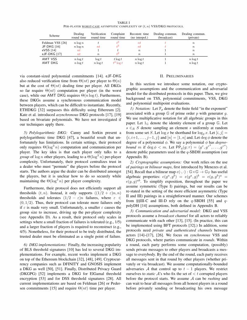
TABLE IPER-PLAYER WORST-CASE ASYMPTOTIC COMPLEXITY OF (t, n) VSS/DKG PROTOCOLS.

Scheme Dealinground time

Verificationround time

Complaintround time

Reconstr. time(no interpol.)

Dealing commun.(broadcast)

Dealing commun.(private)

Feldman VSS [26] n logn t t2 nt t nJF-DKG [16] n logn nt t3 nt t neVSS [14] nt 1 t n 1 neJF-DKG [17] nt n t2 n 1 n

AMT VSS n log t log t t log t n log t 1 n log tAMT DKG n log t n log t t2 log t n log t 1 n log t

via constant-sized polynomial commitments [14]. eJF-DKGalso reduced verification time from Θ(nt) per player to Θ(n)but at the cost of Θ(nt) dealing time per player. All DKGsso far require Θ(nt) computation per player (in the worstcase), while our AMT DKG requires Θ(n log t). Furthermore,these DKGs assume a synchronous communication modelbetween players, which can be difficult to instantiate. Recently,ETHDKG [32] surpasses this difficulty using Ethereum [2].Kate et al. introduced asynchronous DKG protocols [17], [19]based on bivariate polynomials. We have not investigated ifour techniques apply there.

5) Polylogarithmic DKG: Canny and Sorkin present apolylogarithmic time DKG [47], a beautiful result that un-fortunately has limitations. In certain settings, their protocolonly requires Θ(log3 n) computation and communication perplayer. The key idea is that each player only talks to agroup of log n other players, leading to a Θ(log3 n) per-playercomplexity. Unfortunately, their protocol centralizes trust ina dealer who must “permute” the players before the protocolstarts. The authors argue the dealer can be distributed amongstthe players, but it is unclear how to do so securely whilemaintaining the Θ(log3 n) per player complexity.

Furthermore, their protocol does not efficiently support allthresholds (t, n). Instead, it only supports ((1/2 + ε)n, n)thresholds and tolerates (1/2 − ε)n failures, where ε ∈(0, 1/2). Thus, their protocol can tolerate more failures onlyif ε is made very small. Unfortunately, a smaller ε causes thegroup size to increase, driving up the per-player complexity(see Appendix D). As a result, their protocol only scales insettings where a small fraction of failures is tolerated (e.g., 1/5)and a larger fraction of players is required to reconstruct (e.g.,4/5). Nonetheless, for their protocol to be truly distributed, thetrusted dealer must be eliminated as a single point of failure.

6) DKG implementations: Finally, the increasing popularityof BLS threshold signatures [10] has led to several DKG im-plementations. For example, recent works implement a DKGon top of the Ethereum blockchain [32], [48], [49]. Cryptocur-rency companies such as DFINITY and GNOSIS implementa DKG as well [50], [51]. Finally, Distributed Privacy Guard(DKGPG) [52] implements a DKG for ElGamal thresholdencryption [53] and for DSS threshold signatures [28]. Allcurrent implementations are based on Feldman [26] or Peder-sen commitments [15] and require Θ(nt) time per player.

II. PRELIMINARIES

In this section we introduce some notation, our crypto-graphic assumptions and the communication and adversarialmodel for the distributed protocols in this paper. Then, we givebackground on TSS, polynomial commitments, VSS, DKGand polynomial multipoint evaluations.

1) Notation: Let Fp denote the finite field “in the exponent”associated with a group G of prime order p with generator g.We use multiplicative notation for all algebraic groups in thispaper. Let 1G denote the identity element of a group G. Lets ∈R S denote sampling an element s uniformly at randomfrom some set S. Let log x be shorthand for log2 x. Let [i, j] =i, i+1, . . . , j−1, j and [n] = [1, n] and. Let deg φ denote thedegree of a polynomial φ. We say a polynomial φ has degree-bound m if deg φ < m. Let PPq(g; τ) = 〈gτ , gτ2

, . . . , gτq 〉

denote public parameters used in the q-SBDH assumption (seeAppendix B).

2) Cryptographic assumptions: Our work relies on the useof pairings or bilinear maps, first introduced by Menezes et al.[54]. Recall that a bilinear map e(·, ·) : G×G→ GT has usefulalgebraic properties: e(ga, gb) = e(ga, g)b = e(g, gb)a =e(g, g)ab. To simplify exposition, throughout the paper weassume symmetric (Type I) pairings, but our results can bere-stated in the setting of the more efficient asymmetric (TypeII and III) pairings in a straightforward manner. Our schemesfrom §§III-C and III-D rely on the q-SBDH [55] and q-polyDH [14] assumptions, both defined in Appendix B.

3) Communication and adversarial model: DKG and VSSprotocols assume a broadcast channel for all actors to reliablycommunicate with each other [13], [15]. (In practice, this canbe implemented using BFT protocols [32].) In addition, someprotocols need private and authenticated channels betweenactors [14]–[17], [26]. We focus on synchronous VSS andDKG protocols, where parties communicate in rounds. Withina round, each party performs some computation, (possibly)sends private messages to other players and broadcasts a mes-sage to everybody. By the end of the round, each party receivesall messages sent in that round by other players (whether pri-vately or via broadcast). We assume computationally-boundedadversaries A that control up to t − 1 players. We restrictourselves to static A’s who fix the set of < t corrupted playersbefore the protocol starts. We assume A can be rushing andcan wait to hear all messages from all honest players in a roundbefore privately sending or broadcasting his own message

within that same round. The protocols in this paper are robust:there are always t honest players who can reconstruct thesecret. In the synchronous setting, robustness holds for allt− 1 < n/2 [16].

4) FFT and Lagrange interpolation: We use the FastFourier Transform (FFT) to multiply and divide polynomi-als in Fp[X] of degree-bound N = 2k in Θ(N logN)time [56], [57]. For this, we need a primitive N th root ofunity in Fp, which we denote by ωN [56]. Finally, given(xi, yi = φ(xi))i∈[n], interpolating φ takes Θ(n log2 n) timeusing fast Lagrange interpolation [27]. Specifically, recall thatφ(x) =

∑i∈[n] L

[n]i (x)yi where L[n]

i (x) =∏j∈[n]j 6=i

x−xjxi−xj is

called a Lagrange polynomial [58]. Note that L[n]i is defined

with respect to the set of points xii∈[n]. Throughout thispaper, this set will typically be xii∈T where T ⊂ [n], witheither xi = i or xi = ωi−1N and the Lagrange polynomial willbe denoted LTi (x).

A. Threshold Signature Schemes (TSS)

A (t, n)-threshold signature scheme (TSS) is a protocolamongst n signers where only subsets of size ≥ t canproduce a digital signature [59] on a message m. Manysignature schemes can be turned into a TSS, such as RSA [11],[59], Schnorr [20], [60], [61], ElGamal [35]–[37], [62],ECDSA [21] and BLS [10], [63]. In this paper, we focus onthe BLS TSS because of its simplicity and efficiency.

1) (Threshold) BLS signatures: A normal BLS signatureon a message m ∈ 0, 1∗ is σ = H(m)s where s ∈R Fpis the secret key and H : 0, 1∗ → G is a hash functionmodeled as a random oracle. To verify the signature againstthe public key gs, a bilinear map e is used to ensure thate(H(m), gs)

?= e(σ, g)⇔ e(H(m), g)s

?= e(H(m)s, g).

To obtain a (t, n) BLS TSS [10], the secret key s is splitamongst the n signers using (t, n) Shamir secret sharing (see§II-C). Specifically, each signer i has a secret key share si ofs along with a verification key gsi . To produce a signature onm, each i computes a signature share σi = H(m)si . Then, allσi’s are sent to an aggregator (e.g., one of the signers). Sincesome signers are malicious, their σi might not be valid. Thus,the aggregator verifies each σi by checking if e(gsi , H(m))

?=

e(σi, g). (This works because σi is a normal BLS signaturethat should verify under gsi .) This way, the aggregator findsa subset T of t signers who produced a valid signature shareσi. Now, the aggregator can compute the final signature asσ =

∏i∈T σ

LTi (0)i = H(m)

∑i∈T siL

Ti (0) = H(m)s via

Lagrange interpolation (see §II-4). Importantly, aggregationnever exposes the secret key s, which is interpolated “inthe exponent.” The time to aggregate the signature is Θ(t2),dominated by the time to (naively) compute the LTi (0)’s.

B. Constant-sized Polynomial Commitments

Kate, Zaverucha and Goldberg introduced constant-sized polynomial commitments, often called KZG com-mitments [14]. Their scheme requires `-SDH [64] publicparameters PP`(g; τ) = (gτ

i

)i∈[0,`] where τ denotes a

trapdoor. (These parameters are computed via a trustedsetup; see §V-1.) Their scheme is computationally-hiding(see Definition A.5) under the discrete log assumption andcomputationally-binding [14] under `-SDH. Unlike Pedersencommitments [12], KZG can only commit to polynomials ofmaximum degree `.

Let φ denote a polynomial of degree d ≤ ` with coefficientsc0, c1, . . . , cd in Fp. A KZG commitment to φ is a single groupelement C =

∏di=0

(gτ

i)ci

= g∑di=0 ciτ

i

= gφ(τ). Note thatcommitting to φ takes Θ(d) time. To compute an evaluationproof that φ(a) = y, KZG leverages the polynomial remaindertheorem, which says:

φ(a) = y ⇔ ∃q, φ(x)− y = q(x)(x− a) (1)

The proof is just a KZG commitment to q: a single groupelement π = gq(τ). Computing the proof takes Θ(d) time.To verify π, one checks (in constant time) if e(C/gy, g) =e(π, gτ/ga)⇔ e(g, g)φ(τ)−y = e(g, g)q(τ)(τ−a).

1) Batch proofs and homomorphism: Given a set of pointsS and their evaluations φ(i)i∈S , KZG can prove all eval-uations with one constant-sized batch proof rather than |S|individual proofs [14]. The prover computes an accumulatorpolynomial a(x) =

∏i∈S(x − i) in Θ(|S| log2 |S|) time and

computes φ/a in Θ(d log d) time, obtaining a quotient q andremainder r. The batch proof is π = gq(τ). To verify π againstφ(i)i∈S and C, the verifier first computes a from S andinterpolates r such that r(i) = φ(i),∀i ∈ S in Θ(|S| log2 |S|)time. Next, he computes ga(τ) and gr(τ) commitments. Finally,he checks if e(C/gr(τ), g) = e(gq(τ), ga(τ)). We stress thatbatch proofs are only useful when |S| ≤ d. Otherwise, if|S| > d, we can interpolate φ directly from the evaluations,which makes verifying any evaluation trivial.

Finally, KZG proofs have a homomorphic property. Supposewe have two polynomials φ1, φ2 with commitments C1, C2

and two proofs π1, π2 for φ1(a) and φ2(a), respectively. Then,a commitment C to the sum polynomial φ = φ1 + φ2 can becomputed as C = C1C2 = gφ1(τ)gφ2(τ) = gφ1(τ)+φ2(τ) =g(φ1+φ2)(τ). Even better, a proof π for φ(a) w.r.t. C can beaggregated as π = π1π2. This homomorphism is necessary inKZG-based protocols such as eJF-DKG (see §II-D).

C. (Verifiable) Secret Sharing

A (t, n) secret sharing scheme allows a dealer to split upa secret s amongst n players such that only subsets of size≥ t players can reconstruct s. Secret sharing schemes wereintroduced independently by Shamir [65] and Blakley [66].Shamir’s secret sharing (SSS) is split into two phases. Inthe sharing phase, the dealer picks a degree t − 1, random,univariate polynomial φ, lets s = φ(0) and distributes a sharesi = φ(i) to each player i ∈ [n]. In the reconstructionphase, any subset T ⊂ [n] of t honest players can recon-struct s by sending their shares to a reconstructor. For eachi ∈ T , the reconstructor computes a Lagrange coefficientLTi (0) =

∏j∈T,j 6=i

0−ji−j . Then, he computes the secret as

s = φ(0) =∑i∈T LTi (0)si (see §II-4).

Algorithm 1 eVSS: A synchronous (t, n) VSS

Sharing PhaseDealing round:1) The dealer picks φ ∈R Fp[X] of degree t− 1 with s = φ(0), computes

all shares si = φ(i), and commits to φ as c = gφ(τ).2) Computes KZG proofs πi = gqi(τ), qi(x) =

φ(x)−φ(i)x−i , ∀i ∈ [n].

3) Broadcasts c to all players. Then, sends (si, πi) to each player i ∈ [n]over an authenticated, private channel.

Verification round:1) Each player i ∈ [n] verifies πi against c by checking if e(c/gsi , g) =

e(πi, gτ−i). If this check fails (or i received nothing from dealer), then

i broadcasts a complaint against the dealer.Complaint round:1) If the size of the set S of complaining players is ≥ t, the dealer is

disqualified. Otherwise, the dealer reveals the correct shares with proofsby broadcasting si, πii∈S .

2) If any one proof does not verify (or dealer did not broadcast), the dealeris disqualified. Otherwise, each i ∈ [n] now has his correct share si.

Reconstruction PhaseGiven commitment c and shares (i, si, πi)i∈T , |T | ≥ t, the reconstructor:1) Verifies each si, identifying a subset V of t players with valid shares.2) Interpolates s =

∑i∈V LVi (0)si = φ(0).

Unfortunately, SSS does not tolerate malicious dealers whodistribute invalid shares, nor malicious players who mightsend invalid shares during reconstruction. To deal with this,Verifiable Secret Sharing (VSS) protocols enable players toverify shares from a potentially-malicious dealer [12]–[14],[26]. Furthermore, VSS also enables the reconstructor to verifythe shares before interpolating the (wrong) secret. Looselyspeaking, VSS protocols must offer two properties againstany adversary who compromises the dealer and < t players:secrecy and correctness. Secrecy guarantees that no adversarylearns the secret s when the dealer is honest, since a maliciousone can simply reveal s. Correctness guarantees that, after thesharing phase, either any set of ≥ t honest players can alwaysreconstruct s or the dealer is disqualified. We refer the readerto [14] for more formal VSS definitions.

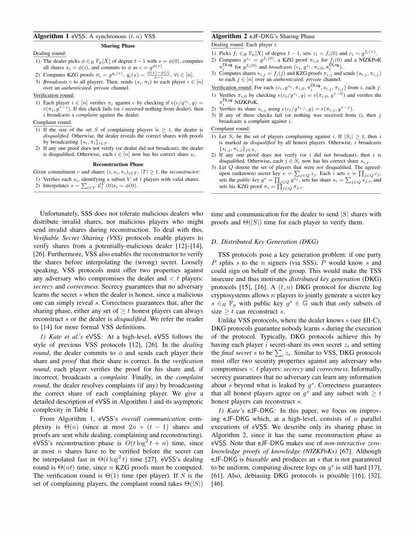
1) Kate et al.’s eVSS: At a high-level, eVSS follows thestyle of previous VSS protocols [12], [26]. In the dealinground, the dealer commits to φ and sends each player theirshare and proof that their share is correct. In the verificationround, each player verifies the proof for his share and, ifincorrect, broadcasts a complaint. Finally, in the complaintround, the dealer resolves complaints (if any) by broadcastingthe correct share of each complaining player. We give adetailed description of eVSS in Algorithm 1 and its asymptoticcomplexity in Table I.

From Algorithm 1, eVSS’s overall communication com-plexity is Θ(n) (since at most 2n + (t − 1) shares andproofs are sent while dealing, complaining and reconstructing).eVSS’s reconstruction phase is O(t log2 t + n) time, sinceat most n shares have to be verified before the secret canbe interpolated fast in Θ(t log2 t) time [27]. eVSS’s dealinground is Θ(nt) time, since n KZG proofs must be computed.The verification round is Θ(1) time (per player). If S is theset of complaining players, the complaint round takes Θ(|S|)

Algorithm 2 eJF-DKG’s Sharing PhaseDealing round: Each player i:

1) Picks fi ∈R Fp[X] of degree t− 1, sets zi = fi(0) and ci = gfi(τ).2) Computes gzi = gfi(0), a KZG proof πi,0 for fi(0) and a NIZKPoK

πDLogi for gfi(0) and broadcasts (ci, g

zi , πi,0, πDLogi ).

3) Computes shares si,j = fi(j) and KZG proofs πi,j and sends (si,j , πi,j)to each j ∈ [n] over an authenticated, private channel.

Verification round: For each (ci, gzi , πi,0, π

DLogi , si,j , πi,j) from i, each j:

1) Verifies πi,0 by checking e(ci/gzi , g) = e(πi,0, gτ−0) and verifies the

πDLogi NIZKPoK.

2) Verifies its share si,j using e(ci/gsi,j , g) = e(πi,j , gτ−j).

3) If any of these checks fail (or nothing was received from i), then jbroadcasts a complaint against i.

Complaint round:1) Let Si be the set of players complaining against i. If |Si| ≥ t, then i

is marked as disqualified by all honest players. Otherwise, i broadcastssi,j , πi,jj∈Si .

2) If any one proof does not verify (or i did not broadcast), then i isdisqualified. Otherwise, each j ∈ Si now has his correct share si,j .

3) Let Q denote the set of players that were not disqualified. The agreed-upon (unknown) secret key s =

∑j∈Q zj . Each i sets c =

∏j∈Q cj ,

sets the public key gs =∏j∈Q g

zj , sets his share si =∑j∈Q sj,i, and

sets his KZG proof πi =∏j∈Q πj,i.

time and communication for the dealer to send |S| shares withproofs and Θ(|S|) time for each player to verify them.

D. Distributed Key Generation (DKG)

TSS protocols pose a key generation problem: if one partyP splits s to the n signers (via SSS), P would know s andcould sign on behalf of the group. This would make the TSSinsecure and thus motivates distributed key generation (DKG)protocols [15], [16]. A (t, n) DKG protocol for discrete logcryptosystems allows n players to jointly generate a secret keys ∈R Fp with public key gs ∈ G such that only subsets ofsize ≥ t can reconstruct s.

Unlike VSS protocols, where the dealer knows s (see §II-C),DKG protocols guarantee nobody learns s during the executionof the protocol. Typically, DKG protocols achieve this byhaving each player i secret-share its own secret zi and settingthe final secret s to be

∑i zi. Similar to VSS, DKG protocols

must offer two security properties against any adversary whocompromises < t players: secrecy and correctness. Informally,secrecy guarantees that no adversary can learn any informationabout s beyond what is leaked by gs. Correctness guaranteesthat all honest players agree on gs and any subset with ≥ thonest players can reconstruct s.

1) Kate’s eJF-DKG: In this paper, we focus on improv-ing eJF-DKG which, at a high-level, consists of n parallelexecutions of eVSS. We describe only its sharing phase inAlgorithm 2, since it has the same reconstruction phase aseVSS. Note that eJF-DKG makes use of non-interactive zero-knowledge proofs of knowledge (NIZKPoKs) [67]. AlthougheJF-DKG is biasable and produces an s that is not guaranteedto be uniform, computing discrete logs on gs is still hard [17],[61]. Also, debiasing DKG protocols is possible [16], [32],[46].

φ = q1,8(x− 1)(x− 2) . . . (x− 8) + r1,8

r1,8 = q1,4(x− 1)(x− 2) . . . (x− 4) + r1,4

r1,4 = q1,2(x− 1)(x− 2) + r1,2

r1,2 = q1,1(x− 1) + r1,1

r1,2 = q2,2(x− 2) + r2,2

r1,4 = q3,4(x− 3)(x− 4) + r3,4

r3,4 = q3,3(x− 3) + r3,3

r3,4 = q4,4(x− 4) + r4,4

r1,8 = q5,8(x− 5)(x− 6) . . . (x− 8) + r5,8

r5,8 = q5,6(x− 5)(x− 6) + r5,6

r5,6 = q5,5(x− 5) + r5,5

r5,6 = q6,6(x− 6) + r6,6

r5,8 = q7,8(x− 7)(x− 8) + r7,8

r7,8 = q7,7(x− 7) + r7,7

r7,8 = q8,8(x− 8) + r8,8

Fig. 1. A multipoint evaluation of polynomial φ at points [8] = 1, 2, . . . , 8. Each node is expressed as a = q · b+ r: i.e., a polynomial a is being dividedby b, resulting in a quotient q and a remainder r. In the root node, φ is divided by the root accumulator

∏i∈[8](x − i), obtaining a quotient q1,8 and a

remainder r1,8. Then, the root’s left child divides r1,8 by (x− 1) · · · (x− 4) while the right child divides it by (x− 5) · · · (x− 8). The process is repeatedrecursively on the resulting r1,4 and r5,8 remainders. The remainders ri,i in the leaves are the evaluations φ(i).

E. Polynomial Multipoint Evaluation

We build upon polynomial multipoint evaluation tech-niques [27]. Given a degree t polynomial φ, naively eval-uating it at n > t points x1, . . . , xn requires Θ(nt) time.This is fast when t is very small relative to n but canbe slow when t ≈ n, as is the case in many instantia-tions of threshold cryptosystems. Fortunately, a multipointevaluation reduces this time to O(n log2 n) using a di-vide and conquer approach. Specifically, one first computesφL(x) = φ(x) mod (x− x1)(x− x2) · · · (x− xn/2) and thenφR(x) = φ(x) mod (x − xn/2+1)(x − xn/2+2) · · · (x − xn)Then, one simply recurses on the two half-sized subprob-lems: evaluating φL(x) at x1, x2, . . . , xn/2 and φR(x) atxn/2+1, xn/2+2, . . . xn. Ultimately, the leaves of this recursivecomputation store φ(x) mod (x − xi), which is exactly φ(i)by the polynomial remainder theorem (see Figure 1).

For example, consider the multipoint evaluation of φ at1, 2, . . . , 8, which we depict in Figure 1. We start at the rootnode ε. Here, we divide φ by the accumulator polynomial (x−1)(x− 2) . . . (x− 8) obtaining a quotient polynomial q1,8 andremainder polynomial r1,8. Then, its left and right children di-vide r1,8 by the left and right “half” of (x−1)(x−2) . . . (x−8),respectively. This proceeds recursively: each node w dividesrparent(w) by its accumulator aw, obtaining a quotient qw andremainder rw such that rparent(w) = qwaw + rw. Note that allaccumulator polynomials aw can be computed in O(n log2 n)time by starting with the (x − i) monomials as leaves of abinary tree and “multiplying up the tree.” Since division by adegree-bound n accumulator takes O(n log n) time, the totaltime is T (n) = 2T (n/2) +O(n log n) = O(n log2 n) [27].

III. SCALABLE THRESHOLD CRYPTOSYSTEMS

First, we show how to speed up and scale threshold sig-nature aggregation as well as secret reconstruction in anyLagrange-based threshold cryptosystem (see §III-A). Then, weintroduce authenticated multipoint evaluation trees (AMTs), anew technique for precomputing logarithmic-sized evaluationproofs much faster in KZG commitments (see §III-B). Last,we use AMTs to speed up and scale Kate et al.’s eVSS andKate’s eJF-DKG (see §§III-C and III-D).

A. Scalable Threshold Signatures

In this section, we show how to reduce the time to aggregatea (t, n) BLS threshold signature from Θ(t2) to Θ(t log2 t).Although we focus on BLS, our techniques can be used inany threshold cryptosystem (not just signatures) whose secretkey lies in a prime-order field Fp. This includes ElGamalsignatures [35]–[37], ElGamal encryption [53] and Schnorrsignatures [20], [61] (but not RSA-based schemes, whosesecret key does not lie in a prime-order field [11]).

Recall from §II-A that BLS TSS aggregation has twophases: (1) computing Lagrange coefficients and (2) exponen-tiating signature shares by these coefficients. Unfortunately, ast gets large, naively computing Lagrange coefficients in Θ(t2)time dominates exponentiating the shares (see Figure 2a). Infact, current descriptions and implementations of thresholdschemes all seem to use this inefficient scheme, which wedub naive Lagrange [10], [38]–[40], [68]. We make threecontributions. First, we adapt the fast polynomial interpolationfrom [27] to compute just the Lagrange coefficients LTi (0) fastin Θ(t log2 t) time. We call this scheme fast Lagrange. Second,we speed up this scheme by using roots of unity rather than1, 2, . . . , n as the signer IDs. Third, we implement a BLSTSS based on fast Lagrange and show it outperforms the naiveone as early as n = 511 (see §IV-A).

1) Fast Lagrange-based BLS: Recall from §II-4 that a La-grange polynomial LTi (x) is defined as LTi (x) =

∏j∈Tj 6=i

x−ji−j .

Let us define N(x) =∏i∈T (x− i). Then, let Ni(x) =

N(x)x−i =

∏j∈T,j 6=i (x− j) be the numerator and let Di =

Ni(i) =∏j∈T,j 6=i (i− j) be the denominator. Now, we can

rewrite LTi (x) = Ni(x)Di

.Our goal is to quickly compute LTi (0) for each signer ID

i ∈ T . In other words, we need to quickly compute all Ni(0)’sand all Di’s. First, given the set of signer IDs T , we interpolateN(x) in Θ(t log2 t) time by starting with the (x − i)’s asleaves of a tree and “multiplying up the tree.” Second, wecan compute all Ni(0) = N(0)/(−i) in Θ(t) time. (Note thatN(0) is just the first coefficient of N(x).) However, computingDi,∀i ∈ T appears to require Θ(t2) time. Fortunately, thederivative N ′(x) of N(x) evaluated at i is exactly equal to

Di [27]. Thus, a Θ(t log2 t) multipoint evaluation of N ′(x) atall i ∈ T can efficiently compute all Di’s!

To see why N ′(i) = Di, it is useful to look at the closedform formula for N ′(x) obtained by applying the product ruleof differentiation (i.e., (fg)′ = f ′g + fg′). For example, forN(x) = (x− 1)(x− 2)(x− 3):

N ′(x) = (x− 2)(x− 3) + (x− 1)(x− 3) + (x− 1)(x− 2)

= N1(x) +N2(x) +N3(x)

In general, we can prove that N ′(x) =∑i∈T Ni(x), where

degN ′ = t − 1. Since Nj(i) = 0 for all i 6= j, it followsthat N ′(i) = Ni(i) + 0 = Di. Lastly, computing N ′(x) onlytakes Θ(t) time via polynomial differentiation. (i.e., N =(ct, ct−1, . . . , c1, c0)⇒ N ′ = (t · ct, (t− 1)ct−1, . . . , 2c2, c1))

To summarize, given a set T of signer IDs, we can computethe Lagrange coefficients LTi (0) = Ni(x)/N ′(i) by (1) com-puting N(x) in Θ(t log2 t) time, (2) computing all Ni(0)’sin Θ(t) time, (3) computing N ′(x) in Θ(t) time and (4)evaluating N ′(x) at all i ∈ T in Θ(t log2 t) time. This reducesthe time to compute all LTi (0)’s from Θ(t2) to Θ(t log2 t).

2) Further speed-ups via roots of unity: The fast Lagrangetechnique works for any threshold cryptosytem whose secretkey s lies in prime-order field Fp. However, for fields thatsupport roots of unity, further speed-ups are possible. (A caveatis that pairings on the underlying elliptic curve can be up to 2×slower.) Without loss of generality, assume the total number ofsigners n is a power of two and let ωn denote a primitive nthroot of unity in Fp. If we replace the 1, . . . , n signer IDswith roots of unity ωi−1n i∈[n], then N ′(x) can be evaluated atany subset of signer IDs with a single Fast Fourier Transform(FFT). This is much faster than a polynomial multipointevaluation, which performs many polynomial divisions, eachinvolving many FFTs. Our fast Lagrange implementation from§IV-A takes advantage of this optimization. Furthermore, weuse roots of unity to compute inverses faster in both our naiveand fast Lagrange implementations (see §IV-A). For example,in naive Lagrange, we compute N(0) =

∏i∈T (0−ωin) much

faster as (−1)|T | · ω∑i∈T i

n .

B. Authenticated Multipoint Evaluation Trees (AMTs)

In this section, we improve KZG’s Θ(nt) time for comput-ing n proofs for a degree-bound t polynomial to Θ(n log t)time. Our key technique is to commit to the quotients ina polynomial multipoint evaluation (see §II-E), obtaining anauthenticated multipoint evaluation tree (AMT). However, ournew AMT evaluation proofs are logarithmic-sized, whereasKZG proofs are constant-sized. As a result, when we applyAMTs to scale VSS and DKG later in §§III-C and III-D,we slightly increase communication complexity and recon-struction time. Nonetheless, in §IV, we demonstrate that thetime saved in proof computation more than makes up forthese smaller increases. Throughout this section, we restrictourselves to computing AMTs at points 1, 2, . . . , n onpolynomials of degree t− 1 < n, since this is the VSS/DKGsetting, (In §V-3, we discuss generalizing to any set of points.)

Finally, in Appendix C, we show AMT evaluation proofs aresecure under q-SBDH. In contrast, KZG proofs are secureunder a weaker assumption called q-SDH [64].

1) Computing AMT proofs: KZG evaluation proofs lever-age the polynomial remainder theorem: ∀i ∈ Fp,∃qi of degreet − 1 such that φ(x) = qi(x)(x − i) + φ(i). Specifically, aconstant-sized KZG proof for φ(i) is just a commitment tothe quotient polynomial qi (see §II-B) and takes Θ(t) time tocompute. Thus, computing KZG proofs for each i ∈ [n] takesΘ(nt) time. We improve on this by looking at φ(x) from thelens of a polynomial multipoint evaluation [27].

For example, consider the multipoint evaluation of φ at alli ∈ [8] from Figure 1. Note that every node in the multipointevaluation tree stores a quotient and a remainder obtainedby dividing the parent node’s remainder by its accumulatorpolynomial (see §II-E). The first key idea is that, for anyevaluation point i ∈ [8], φ(x) can be expressed as φ(i) plus alinear combination of quotients and accumulator polynomialsalong the path to φ(i)’s leaf in the multipoint evaluation tree.For example, consider i = 1, which has the left-most path intree. Start with the root node in Figure 1, which says:

φ(x) = q1,8(x)(x− 1) . . . (x− 8) + r1,8(x)

Then, expand r1,8(x) by going left in the tree (down towardsφ(1)’s leaf), obtaining:

φ(x) = q1,8(x)(x− 1)(x− 2)(x− 3)(x− 4) · · · (x− 8)

+ q1,4(x)(x− 1)(x− 2)(x− 3)(x− 4) + r1,4

Repeat this process recursively by replacing r1,4(x) and thenr1,2(x) to get:

φ(x) = q1,8(x)(x− 1)(x− 2)(x− 3)(x− 4) · · · (x− 8)

+ q1,4(x)(x− 1)(x− 2)(x− 3)(x− 4)

+ q1,2(x)(x− 1)(x− 2)

+ q1,1(x)(x− 1) + φ(1).

Note that φ(x) can be re-expressed similarly for any otherpoints i ∈ [2, n]. Importantly, note that there are only Θ(n)quotient and accumulator polynomials shared by all suchexpressions of φ(i).

Our second key idea follows naturally: we commit to allthese Θ(n) quotient polynomials in the multipoint evaluationof φ. This gives us logarithmic-sized evaluation proofs forany point i ∈ [n]. We call these proofs AMT proofs. Forexample, in Figure 1, the AMT proof for φ(4) would begq1,8(τ), gq1,4(τ), gq3,4(τ), gq4,4(τ), where τ denotes the trap-door used in KZG commitments (see §II-B).

2) Verifying AMT proofs: The next question is how to verifyour new logarithmic-sized AMT proofs. Recall that, given anypoint i, φ(x) can be expressed as:

φ(x) = φ(i) +∑

w∈path(i)

qw(x)aw(x) (2)

where path(i) is the set of nodes along the path from theroot to φ(i) and qw and aw denote the quotient and ac-cumulator polynomials stored at node w in the multipoint

evaluation tree (see Figure 1). How can we verify a proofπi =

(gqw(τ)

)w∈path(i) for φ(i) = yi? We simply use a bilinear

map to check that Equation (2) holds at x = τ :

e(gφ(τ), g)?= e(gyi , g)

∏w∈path(i)

e(gqw(τ), gaw(τ))⇔ (3)

e(g, g)φ(τ)?= e(g, g)yi

∏w∈path(i)

e(g, g)qw(τ)aw(τ) ⇔

e(g, g)φ(τ)?= e(g, g)yi+

∑i∈path(w) qw(τ)aw(τ) ⇔

φ(τ)?= yi +

∑w∈path(i)

qw(τ)aw(τ)

This is reminiscent of how KZG proofs are verified bychecking that φ(x) = qi(x)(x − i) + φ(i) holds at x = τ(see §II-B). However, note that the verifier needs to havethe gaw(τ) accumulator commitments, which are not part ofthe AMT proof. This implies AMT verifiers must have Θ(n)public parameters, whereas KZG verifiers only need gτ astheir public parameters (see §II-B). Fortunately, in §III-B4 wereduce the verifers’ public parameters to just Θ(log t).

3) Better AMTs using roots of unity: Instead of evaluatingφ at points 1, 2, 3, . . . , n, we assume n = 2m and evaluateφ at all n nth roots of unity in Fp. Specifically, we computeφ(ωi−1n ) rather than φ(i), where ωn is a primitive nth root ofunity. (We can generalize to any n by using the first n N throots of unity, where N = 2m is the smallest value such thatN ≥ n.) The main benefit of using roots of unity is they giverise to simpler accumulator polynomials of the form (x2

k

+c)in the multipoint evaluation tree (for some c). This speedsup the multipoint evaluation (see Appendix A), since dividingdegree-bound 2n polynomials by (xn+c) can be done in Θ(n)rather than Θ(n log n) time. In Appendix A, we show this new,optimized AMT proof is blog (t− 1)c+1 group elements andcomputing an AMT takes Θ(n log t) time.

The (x2k

+ c) form of the accumulators is best illustratedwith an example. Let n = 8 and ω8 denote a primitive 8throot of unity. Previously, in Figure 1, the evaluation points1, 2, . . . , 8 were ordered as 〈(x − 1), (x − 2), . . . , (x − 8)〉monomials in the leaves. Then, the accumulators were com-puted by multiplying “up the tree,” culminating in the rootaccumulator

∏i∈[8](x− i). In our case, the evaluation points

are ωi−18 i∈[8] but we reorder them using a bit-reversalpermutation [69] as 〈(x−ω0

8), (x−ω48), (x−ω2

8), (x−ω68), (x−

ω18), (x−ω5

8), (x−ω38), (x−ω7

8)〉. This ordering ensures that,as we multiply “up the tree,” all accumulators are of the form(x2

k

+ ωj8) for some j.Let us see exactly how this happens. The parent accumulator

of the first two leaves (x− ω08) and (x− ω4

8) is their product(x− ω0

8)(x− ω48) = x2 − ω4

8x− ω08x+ ω0

8ω48 . Since ωinω

jn =

ω(i+j) mod nn [56], this equals x2 − x(ω4

8 + ω08) + ω4

8 . Sinceωk+n/2n = −ωkn [56], this equals (x2 + ω4

8). The remainingaccumulators after (x2+ω4

8) on this level are (x2+ω08), (x2+

ω68), (x2 +ω2

8). Recursing on the next level, its accumulatorsare 〈(x4+ω4

8), (x4+ω08)〉. Finally, the root will be (x8−ω0

8) =(x8 − 1) =

∏7i=0(x− ωi8).

4) Do AMTs need extra public parameters?: Recall thatin KZG, given (t − 1)-SDH public parameters, one cancommit to any degree-bound t polynomials and compute anynumber of KZG evaluation proofs. In contrast, computing anAMT at n > t − 1 points seems to require committing todegree n > t − 1 accumulator polynomials (e.g., to the rootaccumulator (xn − 1)). Yet this is not possible given only(t − 1)-SDH parameters, as ensured by the (t − 1)-polyDHassumption (see Appendix B). Fortunately, when computingan AMT, divisions by accumulators of degree > t− 1 alwaysgive quotient zero (see Appendix A). This means that, whenpairing such quotients with their accumulators during proofverification, the result will always be 1GT (see Equation (3)).In other words, such pairings need never be computed andso their corresponding accumulators (of degree > t − 1)need never be committed to. Furthermore, quotients are notproblematic since they always have degree < deg φ = t − 1(or are equal to zero).

Second, AMT verifiers only need a logarithmic number ofgτ

2k

powers to recreate any accumulator commitment gaw(τ).(This is a bit worse than KZG verifiers, who only need gτ .)Specifically, given a subset gτ2k | 0 ≤ k ≤ blog(t− 1)c ofthe (t − 1)-SDH parameters, the verifier can commit to anydegree-bound t accumulator of the (x2

k

+ c) form. Thus, weimpose no additional overhead in the trusted setup. In contrast,if we evaluated φ at 1, 2, . . . , n, verifiers would need all (t−1)-SDH public parameters to reconstruct the accumulators.

C. Scalable Verifiable Secret SharingIn this section, we scale (t, n) VSS protocols to large n

in the difficult case when t > n/2. Specifically, we reduceeVSS’s dealing time from Θ(nt) to Θ(n log t) by replacingKZG proofs with AMT proofs. We call this new VSS protocolAMT VSS and describe it below.

1) Faster dealing: The difference between AMT VSS andeVSS is very small. First, players’ shares are computed assi = φ(ωi−1N ) (rather than φ(i) as in eVSS), where N is thesmallest power of two ≥ n. Second, instead of using (slow)KZG proofs, the dealer computes an AMT for φ at pointsωi−1N i∈[n], obtaining the shares si for free in the process.Then, as in eVSS, the dealer sends each player i its share sibut now with an AMT proof πi (see §III-B1). The verificationround, complaint round and reconstruction phase remain thesame, except they all use AMT proofs now.

AMT VSS’s dealing time is Θ(n log t), dominated by thetime to compute an AMT. This is a significant reduction fromeVSS’s Θ(nt) time, but comes at a small cost due to our largerAMT proofs. First, the verification round time increases fromΘ(1) to Θ(log t). Second, the complaint round complexityincreases from O(t) to O(t log t) time and communication(but we improve it in §III-C2). Third, the reconstruction phasetime increases from Θ(t log2 t+n) to O(t log2 t+n log t) (butwe improve it in §III-C3). Finally, the overall communicationincreases from Θ(n) to Θ(n log t). Nonetheless, in §IV-B,we show AMT VSS’s end-to-end time is much smaller thaneVSS’s, which makes these increases justifiable.

2) Faster complaints: Kate et al. previously point out thatKZG batch proofs (see §II-B1) can be used to reduce thecommunication and the concrete computational complexityof eVSS’s complaint round [14]. Suppose S is the set ofcomplaining players. Without batch proofs, the dealer onlyhas to broadcast |S| previously-computed KZG proofs andeach player has to verify them by computing 2|S| pairings.With batch proofs, the dealer spends Θ(|S| log2 |S| + t log t)time to compute the batch proof and each player spendsΘ(|S| log2 |S|)) to verify it.

While batch proofs increase asymptotic complexity for thedealer and players, the concrete complexity decreases, sinceplayers now only compute two pairings rather than 2|S|.Furthermore, the communication complexity decreases, sinceonly 1 proof rather than |S| needs to be broadcast. Thus,AMT VSS can also use batch proofs and maintain the sameperformance as eVSS during the complaint round. (However,in Table I, we do not assume this optimization.)

3) Efficient reconstruction: In some cases, we can reducethe number of pairings computed during AMT VSS’s re-construction phase. In this phase, the reconstructor is givenanywhere from t to n shares and their AMT proofs. His taskis to find a subset of t valid shares and interpolate the secret.Let us first consider the best case, where all submitted sharesare valid. In this case, if the reconstructor naively verifies anyt AMT proofs, he spends Θ(t log t) time. But he would becomputing the same quotient-accumulator pairings multipletimes (as in Equation (3)), since proofs with intersectingpaths will share quotient commitments. By memoizing thesecomputations, the reconstructor can verify the t proofs in Θ(t)time. Alternatively, this can be sped up by exposing a gs publickey during dealing (as in DKG protocols; see §III-D3).

Now let us consider the worst case, where n − t sharesare invalid and t shares are valid. The reconstructor wants tofind the t valid shares as fast as possible. Once again, he canmemoize the quotient-accumulator pairings that are part ofsuccessfully validated proofs. This way, for the t valid proofs,only Θ(t) pairings need to be computed. Thus, at most Θ((n−t) log t) pairings could possibly be computed for the invalidproofs. The worst-case reconstruction time remains Θ(n log t)but, in practice, the number of pairings is reduced significantlyby the memoization.

4) Public parameters: The AMT VSS dealer needs (t−1)-SDH public parameters, just like in eVSS. This is becausecommitting to accumulator polynomials of degree ≥ t is notnecessary, as discussed in §III-B4. In fact, adding more publicparameters for committing to degree ≥ t polynomials wouldbreak the correctness of eVSS and thus of AMT VSS [14].Specifically, if the dealer commits to a degree ≥ t polynomialφ, then different secrets could be reconstructed, dependingon the subset of players whose shares are used. This iswhy the (t − 1)-polyDH assumption (see Definition A.3) isneeded in both protocols. Finally, AMT VSS players (and thereconstructor) need Θ(log t) public parameters to verify AMTproofs, an increase from eVSS’ Θ(1) (i.e., gτ ).

D. Scalable Distributed Key Generation

In this section, we scale (t, n) DKG protocols to large nin the difficult case when t > n/2. We start from eJF-DKG,where each player acts as an eVSS dealer (see Algorithm 2),taking Θ(nt) time to compute n KZG evaluation proofsand Θ(t) time to compute one KZG proof for gfi(0) (seeAlgorithm 2). We simply replace eVSS with AMT VSS ineJF-DKG, obtaining a new protocol we call AMT DKG withsmaller Θ(n log t) per-player dealing time. Importantly, wekeep the same KZG proof for gfi(0).

Compared to eJF-DKG, AMT DKG has slightly largercommunication (see §IV-C5), larger proof verification timesand a slower complaint round (see Table I). Fortunately, whenusing KZG batch proofs (see §III-C2), the complaint roundcan be made more efficient in both eJF-DKG and AMT DKG.Furthermore, we show AMT DKG players can verify theirshares much faster under certain conditions (see §III-D2).Finally, in §IV-C, we show that our smaller dealing time morethan makes up for these increases.

1) Homomorphic AMT proofs: At the end of eJF-DKG’ssharing phase, each player must aggregate all his shares,commitments and KZG proofs from the set of qualified playersinto a final share, commitment and proof (see Algorithm 2).But for this to work in AMT DKG, AMT proofs must behomomorphic: ∀a ∈ Fp, a proof for f1(a) and a proof forf2(a) must be aggregated into a proof for (f1 + f2)(a).

The key observation is that “adding up” the multipointevaluation trees of two polynomials φ and ρ at the same points(i.e., at X = ωj−1N j∈[n]) results in a multipoint evaluationtree of their sum φ+ ρ (also at X). In more detail, let qw,[ψ]denote the quotient polynomial at node w in ψ’s multipointevaluation tree (at X). Then, one can show that qw,[φ+ρ] =qw,[φ] + qw,[ρ] and that gqw,[φ+ρ](τ) = gqw,[φ](τ)+qw,[ρ](τ) =gqw,[φ](τ)gqw,[ρ](τ). In other words, given an AMT for φ andan AMT for ρ, we can obtain an AMT for φ+ρ by multiplyingquotient commitments at each node. It follows that a proof forf1(a) and one for f2(a) can be aggregated into a proof for(f1 + f2)(a) by multiplying commitments at each node.

2) Fast-track verification round: During the verificationround, each player j must receive and verify shares fromall players i ∈ [n], including himself (see Algorithm 2).Specifically, each player i gives j: (1) a KZG commitmentci of i’s polynomial fi, (2) a share si,j = fi(ω

j−1N ) with an

AMT proof πi,j and (3) gfi(0) with a NIZKPoK and KZGproof. Next, player j must verify each si,j and gfi(0) againsttheir ci. With naive verification, this takes Θ(n log t) pairingsfor all si,j’s (since πi,j’s are AMT proofs), and Θ(n) pairingsfor the gfi(0)’s. We show how batch verification can do thisfaster, with anywhere from Θ(log t) to Θ(n log t) pairings,depending on the number of valid shares. (We will not addressthe Θ(n) work required to verify all NIZKPoKs.)

First, consider the best case when all si,j’s are valid.The key idea is player j will verify just one aggregatedshare sj =

∑ni=1 si,j against an aggregated commitment

call =∏ni=1 ci and aggregated proof πj from all πi,j’s (as

explained in §III-D1). (We ignore the gfi(0)’s for now.) Thistakes Θ(n log t) aggregation work but only takes Θ(log t)pairings. If successful, j has a valid share sj on fall =∑ni=1 fi. The same aggregation can be done on the gfi(0)’s

and their KZG proofs. This way, the number of pairings isreduced significantly to Θ(log t) for the shares and Θ(1) forthe gfi(0)’s. (Again, j still does Θ(n) work to verify theNIZKPoKs individually, which we will not address.)

Since players can be malicious, let us consider an averagecase when a small number of b shares are bad. In this case,j can identify the b shares faster via batch verification [10].Specifically, j starts with the shares, proofs and commitmentsas leaves of a binary tree, where every node aggregates itssubtree’s shares, proofs and commitments. As a result, theroot will contain (call, sj , πj). If verification of the root fails, jproceeds recursively down the tree. Whenever a node verifies,shares in its subtree will no longer be checked individually,saving work for j. In this fashion, j only computes Θ(b log t)pairings if ≤ b shares are bad.

Unfortunately, in the worst case (i.e., t − 1 bad shares),batch verification computes ≈ (2n − 1) log t pairings, whichis slower than the ≈ n log t pairings when done naively. Thus,as pointed out by previous work [70], j should abort and verifynaively after too many nodes fail verification. To summarize, jcan compute fewer pairings by batch-verifying optimisticallyto see if he is in the best or average case and downgradingto naive verification otherwise. We stress that j still doesΘ(n log t) work to build the tree and Θ(n) work to verifyall NIZKPoKs, but fewer (expensive) pairings are computed.

3) Optimistic reconstruction: DKG protocols have the ad-vantage that gs must be exposed to all players and the recon-structor. Thus, the reconstructor can optimistically interpolates from any t shares (without verifying them) and checkthe result against gs. In the best case, when all or mostshares are valid, this will recover the correct s very fast (see§IV-C3). (Note that AMT VSS and eVSS do not expose gs

but they could be easily modified to do so and speed up thereconstruction in the best case, at a very small increase indealing time.) In the worst case, AMT DKG’s reconstructiontime is the same as AMT VSS’s (see §III-C3).

IV. EVALUATION

In this section, we demonstrate the scalability of our pro-posed cryptosystems. Our experiments focus on the difficultcase when t > n/2, specifically t = f+1 and n = 2f+1. Webenchmark TSS, VSS and DKG cryptosystems for thresholdst ∈ 21, 22, 23, . . . , 220. Although we did not benchmarkother thresholds, similar performance gains would have beenobserved for other sufficiently large values of t (e.g., t = f+1and n = 3f + 1). However, we acknowledge that, forsufficiently small t, eVSS’s and eJF-DKG’s Θ(nt) dealingwould outperform ours. Similarly, in this small t setting, naiveLagrange interpolation would outperform fast Lagrange. Ourexperiments show that:• Our BLS TSS scales to n ≈ 2 million signers and outper-

forms the naive scheme as early as n = 511 (see Figure 2a).

• AMT VSS scales to hundreds of thousands of participants,and outperforms eVSS as early as n = 255 (see Figure 2f).

• AMT DKG scales to n ≈ 65,000 players and outperformseJF-DKG at n = 1023 (see Figure 2i).

Importantly, our VSS and DKG speed-ups come at the priceof a modest increase in communication (see Figure 2c). Forexample, for n ≈ 65,000, a DKG player’s communicationduring dealing increases by 4.11× from 18 MiB in eJF-DKGto 74 MiB in AMT DKG. However, since the worst-case end-to-end time decreases by 32× from 16.76 hrs in eJF-DKG to30.83 mins in AMT DKG, the extra communication should beworth it in many applications.

For prohibitively-slow experiments with large t, we repeatthem fewer times than experiments with smaller t. For brevity,we specify the amount of times we repeat an experiment foreach threshold via a measurement configuration. For example,the measurement configuration of our efficient BLS thresholdscheme is 〈7 × 100, 13 × 10〉. This means that for the first7 thresholds t ∈ 21, 22, . . . , 27 we ran the experiment 100times while for the last 13 thresholds we ran it 10 times.

1) Codebase and experimental setup: We implemented (1)our BLS threshold signature scheme from §III-A, (2) eJF-DKG [17] and AMT DKG and (3) eVSS [14] and AMT VSSin 5700 lines of C++. We used a 254-bit Barretto-Naehrigcurve with a Type III pairing [71] from Zcash’s libff [72]elliptic curve library. We used libfqfft [73] to multiplypolynomials fast using FFT. All experiments were run on anIntel Core i7 CPU 980X @ 3.33GHz with 12 cores and 20GB of RAM, running Ubuntu 16.04.6 LTS (64-bit version).Since all benchmarked schemes would benefit equally frommulti-threading, we did not implement it.

2) Limitations: Our DKG and VSS evaluations do notaccount for network delays. This is an important limitation.Our focus was on the computational bottlenecks of theseprotocols. Nonetheless, scaling and evaluating the broadcastchannel of VSS and DKG protocols is necessary, interestingfuture work. In particular, ideas from scalable consensusprotocols [4] could be used for this. Finally, our VSS and DKG“worst case” evaluations do not fully account for maliciousbehavior. Specifically, they do not account for the additionalcommunication and computational cost associated with com-plaint broadcasting. We leave this to future work (see §V-2).

A. BLS Threshold Signature Experiments

First, we sample a random subset of t signers T withvalid signature shares σii∈T . Second, we compute Lagrangecoefficients LTi (0) w.r.t. points xi = ωi−1N (see §II-4) us-ing both fast and naive Lagrange. Third, we compute thefinal threshold signature σ =

∏i∈T σ

LTi (0)i using a multi-

exponentiation. The measurement configuration for fast La-grange is 〈7 × 100, 13 × 10〉 while for naive Lagrange is〈8× 100, 6× 10, 8, 4, 2, 1, 1, 1〉. We plot the average aggrega-tion time in Figure 2a and observe that our scheme beats thenaive scheme as early as n = 511. We do not measure the timeto identify valid signature shares via batch verification [10],which our techniques leaves unchanged.

(a) Threshold signature aggregation time (b) VSS & DKG deal time (c) DKG dealing communication (per player)

(d) VSS verify time (per-player) (e) VSS reconstruction time (f) VSS end-to-end time

(g) DKG verify time (per-player) (h) DKG reconstruction time (i) DKG end-to-end time

Fig. 2. All benchmarked threshold cryptosystems have threshold t = f +1 out of n = 2f +1. The x-axis always indicates log2 t. The y-axis is in seconds,except in Figure 2c it is in MB and in Figure 2d it is in milliseconds.

Our results show that our fast Lagrange interpolation drasti-cally reduces the time to aggregate when t ≈ n/2. Specifically,for n ≈ 221, we aggregate a signature in 46.26 secs, instead of1.59 days if aggregated via naive Lagrange (2964× faster). Thebenefits are not as drastic for smaller thresholds, but remainsignificant. For example, for n ≈ 215, we reduce the time by41× from 29.74 secs to 719.65 ms. For n = 4095, we see a6.6× speed-up from 636.6 ms to 96.17 ms. For n = 2047, wesee a 3× speed-up from 155.62 ms to 50.74 ms.

B. Verifiable Secret Sharing Experiments

In this section, we benchmark eVSS and AMT VSS. We donot benchmark the complaint round since, when implementedwith KZG batch proofs, it remains the same (see §III-C2).

1) VSS dealing: For eVSS dealing, the measurement con-figuration is 〈10 × 10, 3, 2, 2, 1, 1, 0, 0, 0, 0, 0〉. For large t ≥216, eVSS dealing is too slow, so we extrapolate it fromthe previous dealing time (i.e., we multiply by 3.5). ForAMT VSS dealing, the measurement configuration is 〈12 ×100, 50, 22, 10, 5, 3, 2, 1, 1〉. In eVSS, we compute the sharessi “for free” as remainders of the φ(x)/(x− i) divisions. We

plot the average dealing time in AMT VSS and eVSS as afunction of n in Figure 2b. Our results show that AMT VSS’sΘ(n log t) dealing scales much better than eVSS’s Θ(nt)dealing. For example, for n ≈ 65, 000, eVSS takes 15.1 hrswhile AMT VSS takes 1.24 mins. For very large n ≈ 221,eVSS takes a prohibitive 330 days while AMT VSS takes 42mins. We find that AMT VSS’s dealing outperforms eVSS’sas early as n = 31.

2) VSS verification round: In Figure 2d, we plot thetime for one player to verify its share. The measurementconfiguration is 〈20 × 1000〉 for both schemes. In eVSS,verification requires two pairings and one exponentiation inG1, taking on average 2.15 ms. In AMT VSS, verificationrequires blog (t− 1)c + 1 pairings and one exponentiation inG1, ranging from 2.07 ms (n = 3) to 19.85 ms (n ≈ 221).

3) VSS reconstruction: In Figure 2e, we plot the time to re-construct the secret. We consider the best-case and worst-casetimes, as detailed in §III-C3. For eVSS, “best case” means thefirst t share verifications are successful and “worst case” meansthe first n − t are unsuccessful (see §III-C3). The measure-

ment configuration is 〈5× 1000, 500, 250, 120, 60, 30, 15, 5×10, 8, 4, 2, 1〉 for eVSS and 〈9×100, 4×10, 4, 2, 5×1〉 for AMTVSS. In both protocols, the (fast) Lagrange interpolation timeis insignificant compared to the time to verify shares duringreconstruction (e.g., for n ≈ 221 in eVSS, interpolation is only25 secs out of the total 34 mins worst-case time).

AMT VSS’s best-case is very close to eVSS’s worst-case.This is because, with the help of memoization, AMT VSS’sbest case only computes ≤ 2n − 1 pairings (i.e., the numberof nodes in a full binary tree with n leaves). This closelymatches the 2n pairings in eVSS’s worst case. (In practice, wereplace n of these pairings and G1 exponentiations by n GTexponentiations, which are slightly faster.) AMT VSS’s worstcase is 1.12× to 6× slower than eVSS’s. But we show nextthat our faster dealing more than makes up for this. Finally,eVSS’s best-case time is half its worst-case time, as expected.

4) VSS end-to-end time: Finally, we consider the end-to-end time, which is the sum of the sharing and reconstructionphase times. (Again, a limitation of our work is ignoring theoverhead of the complaint round in the worst case.) Figure 2fgives the best- and worst-case end-to-end times. The keytakeaway is that AMT VSS’s smaller dealing time makes upfor the increase in its verification round and reconstructionphase times. AMT VSS outperforms eVSS’s worst-case timeat n ≥ 255 and its best-case time at n ≥ 63. For example,for large n = 16, 383, we reduce the worst-case time from 1.1hrs to 2.9 mins and the best-case time from 1.1 hrs to 51.48secs. The best case improvement ranges from 1.26× (n = 63)to 4484× (n ≈ 221). The worst case improvement ranges from1.26× (n = 255) to 1055× (n ≈ 221). Thus, we conclude AMTVSS scales better than eVSS.

C. Distributed Key Generation Experiments

Our DKG experiments mostly tell the same story as ourVSS experiments: AMTs drastically reduce the dealing timeof DKG players, which more than makes up for the slightincrease in verification and reconstruction time. However,AMT DKG has a 1.2× to 5.2× communication overhead duringdealing. Still, we believe this is worth the drastic reduction inend-to-end times (see §IV-C4).

1) DKG dealing: DKG dealing time is equal to VSSdealing time (see §IV-B1) plus the time to compute a KZGproof and a NIZKPoK for gfi(0). However, as n increases, thetime to compute these two proofs pales in comparison to thetime to compute the n evaluation proofs. Thus, in Figure 2b,we treat DKG dealing times as equal to VSS dealing times.As a result, the same observations apply here as in §IV-B1:AMTs drastically reduce dealing times.

2) DKG verification round: We consider both the best caseand the worst case verification time, as discussed in §III-D2.In our best-case experiment, each player j aggregates all itsshares as sj =

∑i∈[n] si,j and their evaluation proofs as

πj . Then, j verifies sj against πj . Similarly, j aggregatesand efficiently verifies all its gfi(0)’s and their KZG proofs.In the worst-case experiment, j individually verifies the si,jshares and the gfi(0)’s. Importantly, in both experiments, j

individually verifies all n NIZKPoKs for gfi(0) in Θ(n) time.The two experiments are meant to bound the time of a realisticimplementation that carefully uses batch verification [10], [70]to not exceed the worst-case time too much.

The best-case eJF-DKG measurement configuration is〈8 × 100, 50, 25, 12, 9 × 10〉 and the worst-case is 〈5 ×100, 50, 25, 12, 12×10〉. For AMT DKG, the best-case config-uration is 〈12×100, 80, 40, 20, 16, 8, 4, 3, 2〉 and the worst-caseis 〈5×100, 4×80, 40, 20, 8, 4, 2, 6×1〉. The average per-playerverification times are plotted in Figure 2g. In the best case,both schemes perform roughly the same, since the verificationof the n NIZKPoKs quickly starts dominating the aggregatedproof verification. In the worst case, AMT DKG time rangesfrom 8.96 ms (n = 3) to 12.92 hrs (n ≈ 221). In contrast, eJF-DKG time ranges from 8.92 ms to 2.59 hrs (1.5× to 5× faster).Nonetheless, eJF-DKG remains slower overall due to its muchslower dealing (see §IV-C4). Both best- and worst-case timescan be reduced by batch-verifying NIZKPoKs, which resembleSchnorr signatures [60] and are amenable to batching [74].

3) DKG reconstruction: Here the measurement configura-tion is 〈4 × 1000, 200, 50, 25, 13 × 10〉 and times are plottedin Figure 2h. The best case is very fast in both eJF-DKG andAMT DKG, taking only 24.71 secs for t = 220, since bothschemes interpolate the secret s without verifying shares andcheck it against gs (see §III-D3). For the worst case, the timeis the sum of (1) the (failed) best-case reconstruction time and(2) the worst-case time to identify t valid shares from n shares.Since the best case is very fast, the DKG worst-case time (seeFigure 2h) looks almost identical to its VSS counterpart (seeFigure 2e). Note that the same AMT VSS speed-up techniquesfor finding t valid shares apply in AMT DKG (see §III-C3).AMT DKG’s worst case is anywhere from 1.1× to 6× slowerthan eJF-DKG’s, much like AMT VSS. However, as we shownext, AMT DKG’s faster dealing more than makes up for this.

4) DKG end-to-end time: Similar to the VSS experimentsin §IV-B4, we consider the end-to-end time. Figure 2i plotsthe best- and worst-case end-to-end times and shows thatAMT DKG outperforms eJF-DKG starting at n ≥ 63 (in thebest case) and at n ≥ 1023 (in the worst case). This is adirect consequence of AMT VSS outperforming eVSS, sincethe DKG protocols use these VSS protocols internally. Forexample, for large n = 16, 383, we reduce the worst-caseend-to-end time from 1.19 hrs to 7.12 mins and the best-casetime from 1.16 hrs to 25.45 secs. The improvement in best-case end-to-end time ranges from 1.6× (n = 63) to 8607×(n ≈ 221) and, in the worst case, from 1.3× to 427×. Thus,we conclude AMT DKG scales better than eJF-DKG.

5) DKG communication: We estimate each player’s uploadand download during the dealing round. For upload, eacheJF-DKG and AMT DKG player i has to broadcast a KZGcommitment gfi(τ) (32 bytes) and a commitment gfi(0) witha NIZKPoK and a KZG proof (32 + 64 + 32 bytes). Then, ihas to send each j ∈ [n] its share (32 bytes) with an evaluationproof (32 bytes for KZG or (blog (t− 1)c+ 1) · 32 bytes forAMT). For download, each player i, has to download n − 1shares, each with their KZG commitment and evaluation proof,

plus n−1 gfj(0)’s, each with their NIZKPoK and KZG proof.Note that AMT DKG uses KZG proofs for gfi(0) to minimizeits communication overhead.

We plot the upload and download numbers for both schemesin Figure 2c. eJF-DKG’s per-player upload ranges from 288bytes to 128 MiB while download ranges from 448 bytes to448 MiB. AMT VSS’s upload overhead ranges from 1.0×to 10.5× and its download overhead ranges from 1.0× to3.7×. Overall, AMT VSS’s upload-and-download overheadranges from 1.0× to 5.2×. Thus, we believe the 8607× and427× reductions in best- and worst-case end-to-end times aresufficiently large to make up for this overhead.

V. DISCUSSION AND FUTURE WORK

1) Generating public parameters: Similar to eVSS andeJF-DKG, our protocols require a trusted setup to generate`-SDH public parameters. Fortunately, this setup needs to bedone only once and can be securely implemented via MPCprotocols [75], [76]. In fact, currently deployed systems havealready demonstrated the practicality of this approach. In 2018,approximately 200 participants used an MPC [76] to generatenew public parameters for the Sapling version of Zcash [77].The MPC protocol allowed anyone to participate and onlyrequired one honest party, making it a very good candidate.

2) Sortitioned DKG: To further reduce communication andcomputation, we propose a sortitioned DKG where only asmall, random committee of c < n players deal. The keyquestion is where does the randomness to pick the committeecome from? When a DKG runs many times, this randomnesscould come from previous DKG runs (e.g., DKGs for SchnorrTSS nonces). To bootstrap securely, the first DKG run wouldbe with a full committee of size c = n. When a DKG runsonly once, such as when distributing the secret key of a (t, n)TSS, the c players could be a decentralized cothority [41]different than the TSS signers. The cothority would run theDKG dealing round while the n signers would run the DKGverification round (see Algorithm 2). The complaint roundwould be split: accused cothority members would computethe KZG batch proofs (see §III-C2) while the n signerswould receive and verify those proofs. Importantly, our AMTtechnique would help cothority members deal much faster tothe n signers. We leave defining and proving the security ofsortitioned DKGs to future work.

3) Arbitrary points: AMTs can be generalized to any setof points xii∈[n] (not just xi = ωi−1N ) for which verifiers donot have the necessary accumulator commitments. The accu-mulators gaw(τ) can be included as part of the proof but alongwith (1) a subset proof w.r.t. the parent accumulator and (2) an“extractable” counterpart gαaw(τ), where α is another trapdoor.The asymptotic proof size remains the same but will increasein practice by 4x (with Type III pairings). Furthermore, thisconstruction will need extra public parameters of the form(gατ

i

)i∈[0,`]. On the other hand, proof verifiers now needΘ(1) rather than Θ(log n) public parameters (see §§III-B4and III-C4). We leave proving this construction secure under`-PKE [78] to future work.

4) Information-theoretic hiding AMTs: We can devise aninformation-theoretic hiding version of our AMT proofs thatis compatible with information-theoretic hiding KZG com-mitments [14]. This version of AMTs can be used to speedup the unbiasable New-DKG protocol [16]. Let h = gκ beanother generator of G such that nobody knows the discretelog κ = logg(h). Assume that, in addition to PPq(g; τ),we also have public parameters PP`(h; τ). An information-theoretic hiding KZG commitment to φ of degree d is c =gφ(τ)hr(τ) = gφ(τ)+κr(τ) where r is a random, degree dpolynomial [14]. Note that c is just a commitment to thepolynomial ψ(x) = φ(x) + κr(x). As a consequence, all wehave to do is build an AMT for ψ. For this, we compute anAMT for φ with public parameters PP`(g; τ) and one for r butwith parameters PP`(h; τ). By homomorphically combiningthese two AMTs we get exactly the AMT for ψ (see §III-D1).We leave proving this construction is information-theoretichiding to future work.

5) Vector commitments (VCs): AMTs naturally give rise toa VC scheme with logarithmic-sized proofs [79]. Similar tothe multivariate polynomial-based VC from [80], this schemewould also support efficiently updating proofs and updatingVC digests after vector updates. Thus, our VC could also beused for building stateless cryptocurrencies [80], [81]. Our VCcan be extended with zero-knowledge-like properties using theinformation-theoretic variant of AMTs (see §V-4).

6) Batch AMT verification: The efficient reconstructiontechniques from §III-C3 reduced the number of pairings whenverifying an AMT, but still required Θ(t+(n−t) log t) pairingsin the worst case. At the cost of doubling the prover timeand proof size, this can be reduced to ≈ 2n − 1 pairings,independent of how many proofs are valid. The key idea is toalso include commitments to the remainder polynomials fromthe multipoint evaluation tree in the AMT (see Figure 1). Thisway, an entire AMT tree can be verified node-by-node, top-to-bottom by checking that the division at each node is correct.We leave proving this approach secure to future work.

VI. CONCLUSION

We introduced new techniques that both speed up andscale threshold cryptosystems. First, we showed how com-puting Lagrange coefficients efficiently can drastically reducethreshold signature aggregation time. We believe our fast BLSthreshold signature scheme can be used to design simple,large-scale, decentralized random beacons. Second, we intro-duced a quasilinear time technique for precomputing proofsin KZG polynomial commitments. When applied to VSS andDKG protocols, this technique drastically reduces computationwithout increasing communication too much. We left scalingthe broadcast channel and the complaint round to future work.

REFERENCES

[1] S. Nakamoto, “Bitcoin: A Peer-to-Peer Electronic Cash System,” https://bitcoin.org/bitcoin.pdf, 2008, Accessed: 2017-03-08.

[2] G. Wood, “Ethereum: A Secure Decentralised Generalised TransactionLedger,” http://gavwood.com/paper.pdf, Accessed: 2016-05-15.

[3] G. Golan Gueta, I. Abraham, S. Grossman, D. Malkhi, B. Pinkas,M. Reiter, D. Seredinschi, O. Tamir, and A. Tomescu, “SBFT: AScalable and Decentralized Trust Infrastructure,” in DSN’19.

[4] Y. Gilad, R. Hemo, S. Micali, G. Vlachos, and N. Zeldovich, “Algorand:Scaling Byzantine Agreements for Cryptocurrencies,” in ACM SOSP’17.

[5] T. Hanke, M. Movahedi, and D. Williams, “DFINITY TechnologyOverview Series, Consensus System,” CoRR, vol. abs/1805.04548,2018. [Online]. Available: http://arxiv.org/abs/1805.04548

[6] A. Kiayias, A. Russell, B. David, and R. Oliynykov, “Ouroboros: AProvably Secure Proof-of-Stake Blockchain Protocol,” in CRYPTO’17.

[7] B. David, P. Gazi, A. Kiayias, and A. Russell, “Ouroboros Praos: AnAdaptively-Secure, Semi-synchronous Proof-of-Stake Blockchain,” inEUROCRYPT’18.

[8] C. Badertscher, P. Gazi, A. Kiayias, A. Russell, and V. Zikas, “OuroborosGenesis: Composable Proof-of-Stake Blockchains with Dynamic Avail-ability,” in ACM CCS’18.

[9] E. Syta, P. Jovanovic, E. K. Kogias, N. Gailly, L. Gasser, I. Khoffi, M. J.Fischer, and B. Ford, “Scalable Bias-Resistant Distributed Randomness,”in IEEE S&P’17.

[10] A. Boldyreva, “Threshold Signatures, Multisignatures and Blind Signa-tures Based on the Gap-Diffie-Hellman-Group Signature Scheme,” inPKC’03.

[11] V. Shoup, “Practical Threshold Signatures,” in EUROCRYPT’00.[12] T. P. Pedersen, “Non-Interactive and Information-Theoretic Secure Ver-

ifiable Secret Sharing,” in CRYPTO’91.[13] B. Chor, S. Goldwasser, S. Micali, and B. Awerbuch, “Verifiable Secret

Sharing and Achieving Simultaneity in the Presence of Faults,” in IEEEFOCS’85.

[14] A. Kate, G. M. Zaverucha, and I. Goldberg, “Constant-Size Commit-ments to Polynomials and Their Applications,” in ASIACRYPT’10.

[15] T. P. Pedersen, “A Threshold Cryptosystem without a Trusted Party,” inEUROCRYPT’91.

[16] R. Gennaro, S. Jarecki, H. Krawczyk, and T. Rabin, “Secure DistributedKey Generation for Discrete-Log Based Cryptosystems,” Journal ofCryptology, vol. 20, no. 1, 2007.

[17] A. Kate, “Distributed Key Generation and Its Applications,” Ph.D.dissertation, Waterloo, Ontario, Canada, 2010.

[18] C. Cachin, K. Kursawe, and V. Shoup, “Random Oracles in Constantino-ple: Practical Asynchronous Byzantine Agreement Using Cryptography,”Journal of Cryptology, vol. 18, no. 3, Jul 2005.

[19] A. Kate and I. Goldberg, “Distributed Key Generation for the Internet,”in IEEE ICDCS’09.

[20] D. R. Stinson and R. Strobl, “Provably Secure Distributed SchnorrSignatures and a (t, n) Threshold Scheme for Implicit Certificates,” inACISP’01.

[21] R. Gennaro, S. Goldfeder, and A. Narayanan, “Threshold-OptimalDSA/ECDSA Signatures and an Application to Bitcoin Wallet Security,”in ACNS’16.

[22] A. Herzberg, S. Jarecki, H. Krawczyk, and M. Yung, “Proactive SecretSharing Or: How to Cope With Perpetual Leakage,” in CRYPT0’95.

[23] A. Herzberg, M. Jakobsson, S. Jarecki, H. Krawczyk, and M. Yung,“Proactive Public Key and Signature Systems,” in ACM CCS’97.

[24] R. Gennaro, M. O. Rabin, and T. Rabin, “Simplified VSS and Fast-trackMultiparty Computations with Applications to Threshold Cryptography,”in ACM PODC’98.

[25] I. Cascudo and B. David, “SCRAPE: Scalable Randomness Attestedby Public Entities,” in ACNS’17.

[26] P. Feldman, “A Practical Scheme for Non-interactive Verifiable SecretSharing,” in IEEE FOCS’87.

[27] J. von zur Gathen and J. Gerhard, “Fast polynomial evaluation andinterpolation,” in Modern Computer Algebra, 3rd ed. CambridgeUniversity Press, 2013, ch. 10.

[28] R. Canetti, R. Gennaro, S. Jarecki, H. Krawczyk, and T. Rabin, “Adap-tive Security for Threshold Cryptosystems,” in CRYPTO’99.

[29] M. Abe and S. Fehr, “Adaptively Secure Feldman VSS and Applicationsto Universally-Composable Threshold Cryptography,” in CRYPTO’04.

[30] Y. Frankel, P. MacKenzie, and M. Yung, “Adaptively-Secure DistributedPublic-Key Systems,” in Algorithms - ESA’99.

[31] S. Jarecki and A. Lysyanskaya, “Adaptively Secure Threshold Cryp-tography: Introducing Concurrency, Removing Erasures,” in EURO-CRYPT’00.

[32] P. Schindler, A. Judmayer, N. Stifter, and E. Weippl, “ETHDKG: Dis-tributed Key Generation with Ethereum Smart Contracts,” CryptologyePrint Archive, Report 2019/985, 2019, https://eprint.iacr.org/2019/985.

[33] Y. Desmedt, “Society and Group Oriented Cryptography: A New Con-cept,” in CRYPTO’87.

[34] Y. Desmedt and Y. Frankel, “Shared generation of authenticators andsignatures,” in CRYPTO’91.

[35] L. Harn, “Group-oriented (t, n) threshold digital signature schemeand digital multisignature,” IEE Proceedings - Computers and DigitalTechniques, vol. 141, no. 5, Sep. 1994.

[36] C. Park and K. Kurosawa, “New ElGamal Type Threshold DigitalSignature Scheme,” 1996.

[37] R. Gennaro, S. Jarecki, H. Krawczyk, and T. Rabin, “Robust ThresholdDSS Signatures,” in EUROCRYPT’96.

[38] Chia Network, “BLS signatures in C++ using the RELIC toolkit,” https://github.com/Chia-Network/bls-signatures, Accessed: 2019-05-06.

[39] DFINITY, “go-dfinity-crypto,” https://github.com/dfinity/go-dfinity-crypto, Accessed: 2019-05-06.

[40] Mitsunari Shigeo, “BLS threshold signature,” https://github.com/herumi/bls/, Accessed: 2019-05-06.

[41] E. Syta, I. Tamas, D. Visher, D. I. Wolinsky, P. Jovanovic, L. Gasser,N. Gailly, I. Khoffi, and B. Ford, “Keeping Authorities “Honest or Bust”with Decentralized Witness Cosigning,” in IEEE S&P’16.

[42] M. Stadler, “Publicly Verifiable Secret Sharing,” in EUROCRYPT’96.[43] B. Schoenmakers, “A Simple Publicly Verifiable Secret Sharing Scheme

and Its Application to Electronic Voting,” in CRYPTO’99.[44] S. Basu, A. Tomescu, I. Abraham, D. Malkhi, M. K. Reiter, and E. G.

Sirer, “Efficient Verifiable Secret Sharing with Share Recovery in BFTProtocols,” in ACM CCS’19.

[45] I. Ingemarsson and G. J. Simmons, “A Protocol to Set Up SharedSecret Schemes Without the Assistance of a Mutually Trusted Party,”in EUROCRYPT’90.

[46] W. Neji, K. Blibech, and N. Ben Rajeb, “Distributed key generationprotocol with a new complaint management strategy,” SCN’16.

[47] J. Canny and S. Sorkin, “Practical large-scale distributed key genera-tion,” in EUROCRYPT’04.

[48] Philipp Schindler, “Ethereum-based Distributed Key Generation Proto-col,” https://github.com/PhilippSchindler/ethdkg, Accessed: 2019-05-07.

[49] “Orbs Network: DKG for BLS threshold signature scheme on the EVMusing Solidity,” https://github.com/orbs-network/dkg-on-evm, 2018, Ac-cessed: 2019-02-15.

[50] DFINITY, “Distributed Key Generation in JS,” https://github.com/dfinity/dkg, Accessed: 2019-05-07.

[51] GNOSIS, “Distributed Key Generation,” https://github.com/gnosis/dkg,Accessed: 2019-05-07.

[52] Heiko Stamer, “Distributed Privacy Guard,” https://www.nongnu.org/dkgpg/, Accessed: 2019-05-07.

[53] Y. Desmedt and Y. Frankel, “Threshold cryptosystems,” in CRYPTO’89.[54] A. Menezes, S. Vanstone, and T. Okamoto, “Reducing Elliptic Curve

Logarithms to Logarithms in a Finite Field,” in ACM STOC’91.[55] V. Goyal, “Reducing Trust in the PKG in Identity Based Cryptosystems,”

in CRYPTO’07.[56] T. H. Cormen, C. E. Leiserson, R. L. Rivest, and C. Stein, Introduction

to Algorithms, 3rd ed. The MIT Press, 2009.[57] J. von zur Gathen and J. Gerhard, “Newton iteration,” in Modern

Computer Algebra, 3rd ed. Cambridge University Press, 2013, ch. 9.[58] J. Berrut and L. Trefethen, “Barycentric Lagrange Interpolation,” SIAM

Review, vol. 46, no. 3, 2004.[59] R. L. Rivest, A. Shamir, and L. Adleman, “A Method for Obtaining

Digital Signatures and Public-key Cryptosystems,” Commun. ACM,vol. 21, no. 2, Feb. 1978.

[60] C. P. Schnorr, “Efficient Identification and Signatures for Smart Cards,”in CRYPTO’89.

[61] R. Gennaro, S. Jarecki, H. Krawczyk, and T. Rabin, “Secure Applica-tions of Pedersen’s Distributed Key Generation Protocol,” in CT-RSA’03.

[62] T. Elgamal, “A public key cryptosystem and a signature scheme based ondiscrete logarithms,” IEEE Transactions on Information Theory, vol. 31,no. 4, July 1985.

[63] D. Boneh, B. Lynn, and H. Shacham, “Short Signatures from the WeilPairing,” in ASIACRYPT’01.

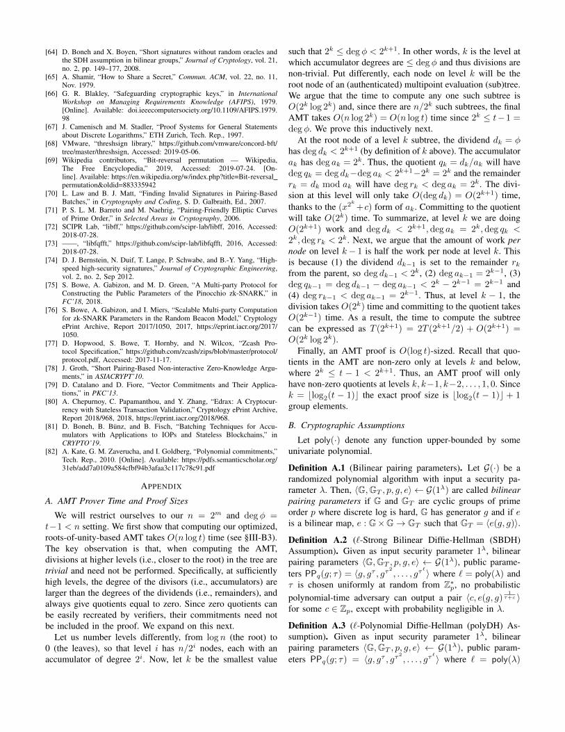
[64] D. Boneh and X. Boyen, “Short signatures without random oracles andthe SDH assumption in bilinear groups,” Journal of Cryptology, vol. 21,no. 2, pp. 149–177, 2008.

[65] A. Shamir, “How to Share a Secret,” Commun. ACM, vol. 22, no. 11,Nov. 1979.

[66] G. R. Blakley, “Safeguarding cryptographic keys,” in InternationalWorkshop on Managing Requirements Knowledge (AFIPS), 1979.[Online]. Available: doi.ieeecomputersociety.org/10.1109/AFIPS.1979.98

[67] J. Camenisch and M. Stadler, “Proof Systems for General Statementsabout Discrete Logarithms,” ETH Zurich, Tech. Rep., 1997.

[68] VMware, “threshsign library,” https://github.com/vmware/concord-bft/tree/master/threshsign, Accessed: 2019-05-06.

[69] Wikipedia contributors, “Bit-reversal permutation — Wikipedia,The Free Encyclopedia,” 2019, Accessed: 2019-07-24. [On-line]. Available: https://en.wikipedia.org/w/index.php?title=Bit-reversalpermutation&oldid=883335942

[70] L. Law and B. J. Matt, “Finding Invalid Signatures in Pairing-BasedBatches,” in Cryptography and Coding, S. D. Galbraith, Ed., 2007.

[71] P. S. L. M. Barreto and M. Naehrig, “Pairing-Friendly Elliptic Curvesof Prime Order,” in Selected Areas in Cryptography, 2006.

[72] SCIPR Lab, “libff,” https://github.com/scipr-lab/libff, 2016, Accessed:2018-07-28.

[73] ——, “libfqfft,” https://github.com/scipr-lab/libfqfft, 2016, Accessed:2018-07-28.

[74] D. J. Bernstein, N. Duif, T. Lange, P. Schwabe, and B.-Y. Yang, “High-speed high-security signatures,” Journal of Cryptographic Engineering,vol. 2, no. 2, Sep 2012.

[75] S. Bowe, A. Gabizon, and M. D. Green, “A Multi-party Protocol forConstructing the Public Parameters of the Pinocchio zk-SNARK,” inFC’18, 2018.

[76] S. Bowe, A. Gabizon, and I. Miers, “Scalable Multi-party Computationfor zk-SNARK Parameters in the Random Beacon Model,” CryptologyePrint Archive, Report 2017/1050, 2017, https://eprint.iacr.org/2017/1050.

[77] D. Hopwood, S. Bowe, T. Hornby, and N. Wilcox, “Zcash Pro-tocol Specification,” https://github.com/zcash/zips/blob/master/protocol/protocol.pdf, Accessed: 2017-11-17.

[78] J. Groth, “Short Pairing-Based Non-interactive Zero-Knowledge Argu-ments,” in ASIACRYPT’10.

[79] D. Catalano and D. Fiore, “Vector Commitments and Their Applica-tions,” in PKC’13.

[80] A. Chepurnoy, C. Papamanthou, and Y. Zhang, “Edrax: A Cryptocur-rency with Stateless Transaction Validation,” Cryptology ePrint Archive,Report 2018/968, 2018, https://eprint.iacr.org/2018/968.

[81] D. Boneh, B. Bunz, and B. Fisch, “Batching Techniques for Accu-mulators with Applications to IOPs and Stateless Blockchains,” inCRYPTO’19.

[82] A. Kate, G. M. Zaverucha, and I. Goldberg, “Polynomial commitments,”Tech. Rep., 2010. [Online]. Available: https://pdfs.semanticscholar.org/31eb/add7a0109a584cfbf94b3afaa3c117c78c91.pdf

APPENDIX

A. AMT Prover Time and Proof Sizes

We will restrict ourselves to our n = 2m and deg φ =t−1 < n setting. We first show that computing our optimized,roots-of-unity-based AMT takes O(n log t) time (see §III-B3).The key observation is that, when computing the AMT,divisions at higher levels (i.e., closer to the root) in the tree aretrivial and need not be performed. Specifically, at sufficientlyhigh levels, the degree of the divisors (i.e., accumulators) arelarger than the degrees of the dividends (i.e., remainders), andalways give quotients equal to zero. Since zero quotients canbe easily recreated by verifiers, their commitments need notbe included in the proof. We expand on this next.

Let us number levels differently, from log n (the root) to0 (the leaves), so that level i has n/2i nodes, each with anaccumulator of degree 2i. Now, let k be the smallest value

such that 2k ≤ deg φ < 2k+1. In other words, k is the level atwhich accumulator degrees are ≤ deg φ and thus divisions arenon-trivial. Put differently, each node on level k will be theroot node of an (authenticated) multipoint evaluation (sub)tree.We argue that the time to compute any one such subtree isO(2k log 2k) and, since there are n/2k such subtrees, the finalAMT takes O(n log 2k) = O(n log t) time since 2k ≤ t−1 =deg φ. We prove this inductively next.

At the root node of a level k subtree, the dividend dk = φhas deg dk < 2k+1 (by definition of k above). The accumulatorak has deg ak = 2k. Thus, the quotient qk = dk/ak will havedeg qk = deg dk−deg ak < 2k+1−2k = 2k and the remainderrk = dk mod ak will have deg rk < deg ak = 2k. The divi-sion at this level will only take O(deg dk) = O(2k+1) time,thanks to the (x2

k

+c) form of ak. Committing to the quotientwill take O(2k) time. To summarize, at level k we are doingO(2k+1) work and deg dk < 2k+1,deg ak = 2k,deg qk <2k,deg rk < 2k. Next, we argue that the amount of work pernode on level k− 1 is half the work per node at level k. Thisis because (1) the dividend dk−1 is set to the remainder rkfrom the parent, so deg dk−1 < 2k, (2) deg ak−1 = 2k−1, (3)deg qk−1 = deg dk−1 − deg ak−1 < 2k − 2k−1 = 2k−1 and(4) deg rk−1 < deg ak−1 = 2k−1. Thus, at level k − 1, thedivision takes O(2k) time and committing to the quotient takesO(2k−1) time. As a result, the time to compute the subtreecan be expressed as T (2k+1) = 2T (2k+1/2) + O(2k+1) =O(2k log 2k).

Finally, an AMT proof is O(log t)-sized. Recall that quo-tients in the AMT are non-zero only at levels k and below,where 2k ≤ t − 1 < 2k+1. Thus, an AMT proof will onlyhave non-zero quotients at levels k, k−1, k−2, . . . , 1, 0. Sincek = blog2(t − 1)c the exact proof size is blog2(t − 1)c + 1group elements.

B. Cryptographic Assumptions

Let poly(·) denote any function upper-bounded by someunivariate polynomial.

Definition A.1 (Bilinear pairing parameters). Let G(·) be arandomized polynomial algorithm with input a security pa-rameter λ. Then, 〈G,GT , p, g, e〉 ← G(1λ) are called bilinearpairing parameters if G and GT are cyclic groups of primeorder p where discrete log is hard, G has generator g and if eis a bilinear map, e : G×G→ GT such that GT = 〈e(g, g)〉.

Definition A.2 (`-Strong Bilinear Diffie-Hellman (SBDH)Assumption). Given as input security parameter 1λ, bilinearpairing parameters 〈G,GT , p, g, e〉 ← G(1λ), public parame-ters PPq(g; τ) = 〈g, gτ , gτ2

, . . . , gτ`〉 where ` = poly(λ) and

τ is chosen uniformly at random from Z∗p, no probabilisticpolynomial-time adversary can output a pair 〈c, e(g, g)

1τ+c 〉

for some c ∈ Zp, except with probability negligible in λ.

Definition A.3 (`-Polynomial Diffie-Hellman (polyDH) As-sumption). Given as input security parameter 1λ, bilinearpairing parameters 〈G,GT , p, g, e〉 ← G(1λ), public param-eters PPq(g; τ) = 〈g, gτ , gτ2

, . . . , gτ`〉 where ` = poly(λ)

and τ chosen uniformly at random from Z∗p, no probabilis-tic polynomial-time adversary can output (φ(x), gφ(τ)) ∈Zp[X]×G, such that 2λ > deg φ > `, except with probabilitynegligible in λ.

C. AMT Proofs are Computationally Hiding and Binding

Recall from [14] that a polynomial commitment schemeconsists of six algorithms: Setup, Commit, Open, VerifyPoly,CreateWitness, VerifyEval. We show our modified KZGscheme with AMT proofs satisfies computational hiding (seeDefinition A.5) under the discrete log (DL) assumption andevaluation binding (see Definition A.4) under the `-StrongBilinear Diffie-Hellman (`-SBDH) assumption. These proper-ties were originally defined in [14]. We prove these propertieshold for a more general scheme that builds AMTs for anarbitrary set X of n points (rather than just for the set ofroots of unity). For this scheme, Setup returns not only `-SDHpublic parameters, but also the accumulator commitmentsnecessary to verify AMT proofs. In other words, given anevaluation point x∗ ∈ X , verifiers have access to accumulatorsgaw(τ)w∈path(x∗) necessary to verify x∗’s AMT proof.

Definition A.4 (Evaluation binding). ∃ negligible functionnegl(·), ∀ security parameters λ, ∀` > 0,∀ adversaries A:

Pr

pp← Setup(1λ, `),

(c, x0, φ(x0), π, φ′(x0), π′)← A(pp) :VerifyEval(pp, c, x0, φ(x0), π) = 1 ∧VerifyEval(pp, c, x0, φ

′(x0), π′) = 1 ∧φ(x0) 6= φ′(x0)

= negl(λ)

Definition A.5 (Computational hiding). Given pp randomlygenerated via Setup(1λ, d), c ∈ G, φ ∈R Fp[X] of de-gree d and (xi, φ(xi), πi)

di=1 for distinct xi’s such that

VerifyEval(pp, c, xi, φ(xi), πi) = 1,∀i ∈ [d], no adversary Acan output φ(x) for any x where x 6= xi,∀i ∈ [d], except withprobability negligible in the security parameter λ.

Computational hiding proof. Suppose there exists an adver-sary A that breaks computational hiding and outputs φ(x) foran unqueried x 6= xi,∀i ∈ [d]. Then, we show how to build anadversary B that takes as input a random discrete log instance(g, ga) and uses A to break it and output a. (Our proof isin the same style as Kate et al.’s proof for PolyCommitDL’scomputational hiding [82].)B runs Setup(1λ, d) which picks τ ∈R Fp and outputs

public parameters pp = PPd(g; τ). Importantly, since B runsthe setup he will know the trapdoor τ . Then, B picks randompoints (xi, yi) ∈ X × Fp,∀i ∈ [0, d] with distinct xi’s,except he sets y0 = a. (Since B does not know a, he justsets gy0 = ga.) Note that (xi, yi)

di=0 determines a degree d

polynomial φ where φ(xi) = yi,∀i ∈ [0, d]. Since B does notknow a (only ga), it will interpolate φ’s commitment gφ(τ)

“in the exponent” as:

gφ(τ) =∏i∈[0,d]

(gyi)LTi (τ)

Here T = xii∈[0,d] and recall that LTi (τ) =∏j∈T,j 6=i(τ −

xj)/(xi − xj) (see §II-4). To summarize, B “embeds” the(g, ga) challenge in an (unknown-to-B-but-determined) poly-nomial φ with commitment c = gφ(τ).

Next, B has to simulate AMT proofs πi for yi = φ(xi),∀i ∈[d]. To do this, recall that at each node w in the AMT, wehave quotient and remainder polynomials qw, rw such thatrparent(w) = qwaw + rw (see Figure 1). Also, recall that Bknows τ so he can compute accumulator evaluations aw(τ),∀nodes w in the AMT. Now, B can simulate proofs as follows.

For the root node w = ε, we have rparent(ε) = φ, so Bpicks a random rε(τ) ∈ Fp, and computes the root quotientcommitment as gqε(τ) = (gφ(τ)/grε(τ))

1aε(τ) . At the next level,

consider the children nodes u and v of the root ε. For eachchild w ∈ u, v, B must commit to a quotient qw that satisfiesrε(τ) = qw(τ)aw(τ) + rw(τ) for some rw. So B proceedssimilarly: for each child w ∈ u, v, he picks a random rw(τ)

and computes a commitment gqw(τ) = (grε(τ)/grw(τ))1

aw(τ) .B will do this recursively until it reaches leaf nodes in theAMT. For each leaf l, instead of picking rl(τ) randomly, Bwill set it to the yi corresponding to that leaf. This way, Bcan simulate quotient commitments gqw(τ)w∈path(xi) for alli ∈ [d] that pass the AMT proof verification in Equation (3).

Next, B calls A with (pp, c, (xi, yi, πi)di=1) as input, hoping

that A outputs another point x and its evaluation φ(x).Since A breaks computational hiding, this happens with non-negligible probability. (Note that B can check A succeeds byinterpolating gφ(x) “in the exponent”.) When A succeeds, ifx = x0, then a = φ(x), so B breaks discrete log on (g, ga).Otherwise, B uses the first d points (xi, yi = φ(xi))i∈[d] andthis new distinct (x, φ(x)) point to interpolate φ and as a resultobtain a = φ(x0). (Recall that, by Definition A.5, we havex 6= xi,∀i ∈ [d].) As a result, B breaks discrete log on (g, ga).Evaluation binding proof. Suppose there exists an adversaryA that outputs a commitment c, with two contradicting proofsπ, π′ attesting that φ(k) is equal to v and v′, respectively.We show how to build another adversary B that breaks q-SBDH. First, B runs A to get (c, π, π′, φ(k), v, v′). Let W =path(k) denote the nodes along k’s path in the AMT. Let(πi)i∈W denote the quotient commitments in π. Similarly, let(π′i)i∈W denote the quotient commitments in π′. Since bothproofs verify, we have:

e(c, g) = e(gv, g)∏i∈W

e(πi, gai(τ))

e(c, g) = e(gv′, g)

∏i∈W

e(π′i, gai(τ))

Dividing the first equation by the second, we get:

1GT =e(gv, g)

e(gv′ , g)

∏i∈W e(πi, g

ai(τ))∏i∈W e(π′i, g

ai(τ))⇔

1GT = e(gv−v′, g)

∏i∈W

e(πi, gai(τ))

e(π′i, gai(τ))

⇔

e(gv′−v, g) =

∏i∈W

e(πi/π′i, g

ai(τ))

Now, recall that one of the accumulators (ai(x))i∈W isthe monomial (x − k), and all the other ai(x)’s contain(x − k) as a term, which means it can be factored out ofthem. Thus, since (x − k) perfectly divides all ai(x)’s, letri(x) = ai(x)/(x − k),∀i ∈ W . Importantly, the adversaryB can compute all ri(x)’s in polynomial time, since it canreconstruct all the accumulator polynomials (ai(x))i∈W . As aresult, B can compute all commitments (gri(τ))i∈W . Then, Bbreaks `-SBDH as follows:

e(gv′−v, g) =

∏i∈W

e(πi/π′i, g

ri(τ)(τ−k))

e(gv′−v, g) =

∏i∈W

e(πi/π′i, g

ri(τ))(τ−k)

e(gv′−v, g) =

[∏i∈W

e(πi/π′i, g

ri(τ))

](τ−k)

e(g, g)1

τ−k =

[∏i∈W

e(πi/π′i, g

ri(τ))

] 1v′−v

D. Polylogarithmic DKG Configurations

As discussed in §I-A, Canny and Sorkin presented a sparsematrix DKG with O(m3) time and communication per player,where m is a group size [47]. Depending on the desiredthreshold (t, n) and the number f of malicious nodes tolerated,the group size m can be as small as Θ(log3(n)). Unfortunately,for f sufficiently close to t, the group size becomes too large,approaching n/2 (see Table II).

TABLE IITHE GROUP SIZE m AND FOR VARIOUS (t, n) SPARSE MATRIX DKGS

WITH f FAILURES TOLERATED.

ε Group size m f = (1/2− ε)n t = (1/2 + ε)n n

0.1 50,598 26,214 39,321 65,5360.15 14,222 22,937 42,598 65,5360.2 5,691 19,660 45,875 65,536

0.25 2,735 16,384 49,152 65,5360.3 1,475 13,107 52,428 65,536

0.33 1,057 11,141 54,394 65,5360.4 505 6,553 8,982 65,536

0.05 445,909 471,859 576,716 1,048,5760.1 53,022 419,430 629,145 1,048,576

0.15 14,949 367,001 681,574 1,048,5760.2 5,977 314,572 734,003 1,048,576

0.25 2,871 262,144 786,432 1,048,5760.3 1,548 209,715 838,860 1,048,576

0.33 1,107 178,257 870,318 1,048,5760.4 527 104,857 943,718 1,048,576