towards the next generation of location-aware communications · towards the next generation of...
TRANSCRIPT

Towards the Next Generation of
Location-Aware Communications
Zohair M. Abu-Shaban
M.Sc. (Imperial College London), D.I.C., B.Eng.
April, 2018
A thesis submitted for the degree of
Doctor of Philosophyof The Australian National University
Any application of the ANU logo on a coloured background is subject to approval by the Marketing Of!ce. Please send to [email protected]
Research School of EngineeringCollege of Engineering and Computer Science
The Australian National University
© Zohair Abu-Shaban, 2018
All Right Reserved


i
Dedicated to my loving wife, Rola
and
our dear children, Mustafa and Elsy.

Declaration
The content of this thesis is the result of original research and have not been
submitted for a higher degree to any other university or institution. Much of this
work has either been published or submitted for publications as journal papers and
conference proceedings. Following is a list of these papers.
Journal Publications
� Z. Abu-Shaban, X. Zhou, T. Abhayapala, “A Novel TOA-based Mobile Lo-
calization Technique under Mixed LOS/NLOS Conditions for Cellular Net-
works,” IEEE Transactions on Vehicular Technology, vol. 65, no. 11, pp.
8841-8853, Nov 2016.
� Z. Abu-Shaban, X. Zhou, T. Abhayapala, G. Seco-Granados, H. Wymeer-
sch, “Error Bounds for Uplink and Downlink 3D Localization in 5G mmWave
Systems,” Accepted in IEEE Transactions on Wireless Communication, April
2018.
� Z. Abu-Shaban, H. Wymeersch, T. Abhayapala, G. Seco-Granados, “Single-
Anchor Two-Way Localization Bounds for 5G mmWave Systems: Two Pro-
tocols,” to be submitted to IEEE Transactions on Wireless Communication,
May 2018.
Conference Proceedings
� Z. Abu-Shaban,H. Wymeersch, X. Zhou, G. Seco-Granados, T. Abhaya-
pala “Random-Phase Beamforming for Initial Access in the Millimeter-Wave
Cellular Networks” in the proceedings of 2016 IEEE Global Communications
Conf. (GLOBECOM), Washington, DC, pp. 1-6, Dec 2016.
iii

iv
� Z. Abu-Shaban, X. Zhou, T. Abhayapala, G. Seco-Granados, H. Wymeer-
sch “Location and Orientation Estimation Performance with Uplink and
Downlink 5G mmWave Multipath Signals” in the proceedings of IEEE Wire-
less Communications and Networking Conf. (WCNC), Barcelona, Spain,
April 2018.
� Z. Abu-Shaban, H. Wymeersch, T. Abhayapala, G. Seco-Granados, “Single-
Anchor Two-Way Localization Bounds for 5G mmWave Systems,” to be sub-
mitted to 2018 IEEE Global Communications Conf. (GLOBECOM Work-
shops), Abu Dhabi, UAE, Dec 2018.
The following papers are also results of my Ph.D. study, but not included in
this thesis:
Journal Publications
� R. Mendrzik, , H. Wymeersch, G. Bauch, Z. Abu-Shaban, “Harnessing
NLOS Components for Position and Orientation Estimation in 5G mmWave
MIMO,” Second round of review after major revisions at IEEE Transactions
on Wireless Communication, Nov 2017.
Conference Proceedings
� T. Abhayapala, H. Chen, Z. Abu-Shaban, “Three Dimensional Beamform-
ing for 5G Networks Using Planar (2D) Antenna Arrays,” To be submitted
European Signal Processing Conference (EUSIPCO), Feb 2018.
The research work presented in this thesis has been performed jointly with Prof.
Thushara D. Abhayapala (ANU), Dr. Xiangyun Zhou (ANU), Prof. Henk Wymeer-
sch (Chalmers, Sweden), and Prof. Gonzalo Seco-Granados (UAB, Spain). At
least, 75% of this work is my own.
Zohair Abu-Shaban
Research School of Engineering
The Australian National University
Canberra ACT 2601
April, 2018
Acknowledgments
First and foremost, all praise belongs to God, who has always been there to give
me guidance, patience and endurance to keep going. Furthermore, this work would
not have been possible, without the support of many people, and for that I would
like to express my gratitude, and acknowledge each and every one of them:
� My supervisor Prof. Thushara Abhayapala for his solid support for me during
my PhD, starting from the application process, arranging a top-up scholar-
ship, to finally writing my thesis. I appreciate him giving me confidence and
freedom to be an independent researcher eventually. Moreover, I enjoyed
learning from his wisdom during our informal tea chats.
� My co-supervisor, Dr. Sean Zhou, for his thought-provoking opinions and
constructive criticism that gave me other angles to look into my work.
� My research collaborator, Prof. Henk Wymeersch, of Chalmers University
of Technology, Sweden, for providing timely and eye-opining feedback on my
work, helping me penetrate a research field that is still in its infancy, and
providing me with a stimulating research environment during my visit to his
group.
� My research collaborator, Prof. Gonzalo Seco-Granados, of the Universitat
Autonoma de Barcelona, Spain, for his research collaboration, which was
instrumental to my work, for his friendly and welcoming attitude when I
visited his research group, and for providing accommodation for me and my
family during that visit.
� The Australian National University (ANU), and the Australian Government’s
v

vi
Research Training Program (RTP) for granting me generous scholarships to
help me realize my dream of pursuing a PhD.
� The Vice-Chancellor of ANU, and the Dean of the ANU’s College of Engi-
neering and Computer Science, for partially sponsoring me with a 4-month
travel grant to pursue overseas research visits that were a crucial stage during
my PhD.
� My colleagues and fellow PhD students in CECS, for being a source of inspi-
ration, and advice whenever I needed them.
� My strong and unique parents, Mustafa and Sawsan, for their endless and un-
conditioned love and support, for having high expectations of me and pushing
me to excel in every task I do. I cannot thank them enough for that.
� Last but not least, the love of my life, Rola and our two children, Mustafa
and Elsy. Having been surrounded by their love, encouragement, patience,
and understanding, they never failed to turbo-charge me to do my best. For
that, I consider them to be the “angel” co-authors of this thesis.

Abstract
This thesis is motivated by the expected implementation of the next generation
mobile networks (5G) from 2020, which is being designed with a radical paradigm
shift towards millimeter-wave technology (mmWave). Operating in 30–300 GHz
frequency band (1–10 mm wavelengths), massive antenna arrays that provide a
high angular resolution, while being packed on a small area will be used. More-
over, since the abundant mmWave spectrum is barely occupied, large bandwidth
allocation is possible and will enable low-error time estimation. With this high
spatiotemporal resolution, mmWave technology readily lends itself to extremely
accurate localization that can be harnessed in the network design and optimiza-
tion, as well as utilized in many modern applications. Localization in 5G is still in
early stages, and very little is known about its performance and feasibility.
In this thesis, we contribute to the understanding of 5G mmWave localiza-
tion by focusing on challenges pertaining to this emerging technology. Towards
that, we start by considering a conventional cellular system and propose a posi-
tioning method under outdoor LOS/NLOS conditions that, although approaches
the Cramer-Rao lower bound (CRLB), provides accuracy in the order of meters.
This shows that conventional systems have limited range of location-aware appli-
cations. Next, we focus on mmWave localization in three stages. Firstly, we tackle
the initial access (IA) problem, whereby user equipment (UE) attempts to estab-
lish a link with a base station (BS). The challenge in this problem stems from the
high directivity of mmWave. We investigate two beamforming schemes: directional
and random. Subsequently, we address 3D localization beyond IA phase. Devices
nowadays have higher computational capabilities and may perform localization in
the downlink. However, beamforming on the UE side is sensitive to the device
orientation. Thus, we study localization in both the uplink and downlink under
vii

viii
multipath propagation and derive the position (PEB) and orientation error bounds
(OEB). We also investigate the impact of the number of antennas and the number
of beams on these bounds. Finally, the above components assume that the system
is synchronized. However, synchronization in communication systems is not usu-
ally tight enough for localization. Therefore, we study two-way localization as a
means to alleviate the synchronization requirement and investigate two protocols:
distributed (DLP) and centralized (CLP).
Our results show that random-phase beamforming is more appropriate IA ap-
proach in the studied scenarios. We also observe that the uplink and downlink are
not equivalent, in that the error bounds scale differently with the number of anten-
nas, and that uplink localization is sensitive to the UE orientation, while downlink
is not. Furthermore, we find that NLOS paths generally boost localization. The
investigation of the two-way protocols shows that CLP outperforms DLP by a sig-
nificant margin. We also observe that mmWave localization is mainly limited by
angular rather than temporal estimation.
In conclusion, we show that mmWave systems are capable of localizing a UE
with sub-meter position error, and sub-degree orientation error, which asserts that
mmWave will play a central role in communication network optimization and un-
lock opportunities that were not available in the previous generation.

List of AcronymsBS Base Station
CDF Cumulative Distribution Function
CLP Centralized Localization Protocol
CRLB Cramer-Rao lower bound
DBF Directional Beamforming
DLP Distributed Localization Protocol
DOA Direction-of-Arrival
DOD Direction-of-Departure
(E)FIM (Equivalent) Fisher Information Matrix
IA Initial Access
mmWave Millimeter-wave Technology
MSE Mean Square Error
(N)LOS (None-)line-of-sight
OEB Orientation Error Bound
PDF Probability Density Function
PEB Position Error Bound
PSD Power Spectral Density
RMSE Root Mean Square Error
RPBF Random-Phase Beamforming
RSS Received Signal Strength
SNR Signal-to-Noise Ratio
TDOA Time-Difference-of-Arrival
TOA Time-of-Arrival
UE User Equipment
ULA Uniform Linear Array
URA Uniform Rectangular Array
ix


Notations and Symbolsj
√−1
a Scalar
a Column vector
A Matrix
[A]m,n Element in the mth row and nth column of A
(·)T Vector and matrix transpose operator
(·)H Vector and matrix complex conjugate transpose operator
det(A) Determinant of a square matrix
diag(A) Diagonal of a square matrix
diag(a) Square matrix with a as main diagonal
Tr(A) Trace of a square matrix
‖ · ‖ `2 norm of a vector
‖ · ‖F Frobenius norm of a matrix
0N All-zeros column vector of length N
0N×N All-zeros matrix of size N ×N1N All-ones column vector of length N
1N×N All-ones matrix of size N ×NIN Identity matrix of size N ×NE{·} Expectation operator
<{·} Real part
={·} Imaginary part
� Hadamard product
⊗ Kronecker product
RN N -dimensional real vector space
RN×M N ×M dimensional real matrix space
CN N -dimensional complex vector space
CN×M N ×M dimensional complex matrix space
xi
xii
λ Wavelength
c Speed of light (= 3× 10⁸)
τ Time-of-arrival
β Complex path gain
θ Elevation angle measure w.r.t positive z-axis
φ Azimuth angle measure w.r.t positive x-axis
aR(θ, φ) Receiver array response vector in the direction (θ, φ)
aT(θ, φ) Transmitter array response vector in the direction (θ, φ)
k(θ, φ) Wavenumber vector in the direction (θ, φ)
p User equipment position.
o User equipment orientation.
F Transmit beamforming matrix.
W Receive beamforming matrix.
s(t) Transmitted signal vector.
r(t) Received signal vector at the antenna array.
y(t) Received signal vector after receive beamforming.
ϕ Vector of unknown parameters.
ϕ Estimator of ϕ.
Jϕ Fisher Information Matrix of ϕ.
Jeϕ Equivalent Fisher Information Matrix of ϕ.
Υ Parameter transformation matrix.
B Clock bias of the clock of D2 w.r.t the clock of D1.
W System bandwidth
Weff Effective bandwidth
Et Transmitted energy per symbol.
Ts Symbol duration.
N0 Noise power spectral density.
NR Number of antennas at the receiver.
NT Number of antennas at the transmitter.
NB Number of transmitted beams.
Ns Number of pilot symbols or measurements.
fX(x) Probability density function of a random variable x.

Contents
Declaration iii
Acknowledgements v
Abstract vii
List of Acronyms ix
Notations and Symbols xi
List of Figures xix
List of Tables xxv
1 Introduction 1
1.1 Evolution of Localization . . . . . . . . . . . . . . . . . . . . . . . . 1
1.2 Classification of Localization Systems . . . . . . . . . . . . . . . . . 3
1.3 Challenges Facing Localization Systems . . . . . . . . . . . . . . . . 9
1.4 5G: Localization Opportunities and Challenges . . . . . . . . . . . . 10
1.5 Thesis Scope and Overview . . . . . . . . . . . . . . . . . . . . . . 13
2 Background Concepts 17
2.1 Background on Array Signal Processing . . . . . . . . . . . . . . . . 18
2.1.1 Array Manifold Vector . . . . . . . . . . . . . . . . . . . . . 18
2.1.2 Analog Beamforming . . . . . . . . . . . . . . . . . . . . . . 22
2.1.3 Received Signal Model . . . . . . . . . . . . . . . . . . . . . 24
2.2 Introduction to Classical Estimation Theory . . . . . . . . . . . . . 26
xiii

xiv Contents
2.2.1 Measurement Model . . . . . . . . . . . . . . . . . . . . . . 27
2.2.2 Estimation Performance . . . . . . . . . . . . . . . . . . . . 27
2.2.3 Cramer-Rao lower bound (CRLB) . . . . . . . . . . . . . . . 28
2.2.4 Transformation of Parameters . . . . . . . . . . . . . . . . . 31
2.2.5 Equivalent Fisher Information Matrix (EFIM) . . . . . . . . 33
2.3 Summary . . . . . . . . . . . . . . . . . . . . . . . . . . . . . . . . 34
3 Mobile Localization under LOS/NLOS Conditions in Conventional
Networks 35
3.1 Introduction . . . . . . . . . . . . . . . . . . . . . . . . . . . . . . . 36
3.2 Problem Formulation . . . . . . . . . . . . . . . . . . . . . . . . . . 39
3.2.1 Assumptions . . . . . . . . . . . . . . . . . . . . . . . . . . . 39
3.2.2 Signal Model . . . . . . . . . . . . . . . . . . . . . . . . . . 40
3.3 Closed-Form NLOS Range Estimation . . . . . . . . . . . . . . . . 42
3.3.1 Range Estimator . . . . . . . . . . . . . . . . . . . . . . . . 42
3.3.2 Range Estimator Error Analysis . . . . . . . . . . . . . . . . 45
3.4 Localization Based on Range Estimates . . . . . . . . . . . . . . . . 47
3.5 Cramer-Rao Lower Bound . . . . . . . . . . . . . . . . . . . . . . . 49
3.6 Numerical Results and Discussion . . . . . . . . . . . . . . . . . . . 53
3.6.1 Simulation Setup . . . . . . . . . . . . . . . . . . . . . . . . 53
3.6.2 Range Estimation . . . . . . . . . . . . . . . . . . . . . . . . 54
3.6.3 Location Estimation . . . . . . . . . . . . . . . . . . . . . . 59
3.7 Conclusions . . . . . . . . . . . . . . . . . . . . . . . . . . . . . . . 62
4 Beamforming for Initial Access in 5G mmWave Networks 65
4.1 Introduction . . . . . . . . . . . . . . . . . . . . . . . . . . . . . . . 65
4.2 Problem Formulation . . . . . . . . . . . . . . . . . . . . . . . . . . 67
4.3 Beamforming: Random-Phase and Directional . . . . . . . . . . . . 70
4.4 Cramer-Rao Lower Bound . . . . . . . . . . . . . . . . . . . . . . . 71
4.4.1 DBF Analysis . . . . . . . . . . . . . . . . . . . . . . . . . . 72
4.4.2 RPBF Analysis . . . . . . . . . . . . . . . . . . . . . . . . . 73
4.5 Simulation and Numerical Results . . . . . . . . . . . . . . . . . . . 74
4.5.1 Effect of NB on the CRLBs of Channel Parameters . . . . . 75
Contents xv
4.5.2 Effect of NR on the CRLBs of Channel Parameters . . . . . 76
4.5.3 Effect of NT on the CRLB . . . . . . . . . . . . . . . . . . . 77
4.5.4 Summary of Results . . . . . . . . . . . . . . . . . . . . . . 77
4.6 Conclusion . . . . . . . . . . . . . . . . . . . . . . . . . . . . . . . . 78
5 Uplink and Downlink 3D Localization Error Bounds in 5G mmWave
Systems 81
5.1 Introduction . . . . . . . . . . . . . . . . . . . . . . . . . . . . . . . 82
5.2 Problem Formulation . . . . . . . . . . . . . . . . . . . . . . . . . . 84
5.2.1 System Geometry . . . . . . . . . . . . . . . . . . . . . . . . 84
5.2.2 Channel Model . . . . . . . . . . . . . . . . . . . . . . . . . 85
5.2.3 Transceiver Model . . . . . . . . . . . . . . . . . . . . . . . 86
5.2.4 3D Localization Problem . . . . . . . . . . . . . . . . . . . . 87
5.3 FIM of The Channel Parameters . . . . . . . . . . . . . . . . . . . 87
5.3.1 Exact Expression . . . . . . . . . . . . . . . . . . . . . . . . 87
5.3.2 Approximate FIM of the Channel Parameters . . . . . . . . 89
5.3.3 FIM of Single-Path mmWave Channel Parameters . . . . . . 92
5.4 FIM of the Location Parameters . . . . . . . . . . . . . . . . . . . . 95
5.4.1 PEB and OEB: Exact Approach . . . . . . . . . . . . . . . . 95
5.4.2 PEB and OEB: Approximate Approach . . . . . . . . . . . . 98
5.4.3 Closed-Form Expressions for LOS: 3D and 2D . . . . . . . . 100
5.5 Numerical Results and Discussion . . . . . . . . . . . . . . . . . . . 102
5.5.1 Simulation Environment . . . . . . . . . . . . . . . . . . . . 102
5.5.2 Tx and Rx Factors of the Approximate FIM . . . . . . . . . 107
5.5.3 Downlink PEB and OEB . . . . . . . . . . . . . . . . . . . . 107
5.5.4 The Selection of NB . . . . . . . . . . . . . . . . . . . . . . 109
5.5.5 Downlink vs. Uplink Comparison . . . . . . . . . . . . . . . 111
5.5.6 Summary of Results . . . . . . . . . . . . . . . . . . . . . . 115
5.6 Conclusions . . . . . . . . . . . . . . . . . . . . . . . . . . . . . . . 116
6 Two-Way Localization Bounds for 5G mmWave Systems 119
6.1 Introduction . . . . . . . . . . . . . . . . . . . . . . . . . . . . . . . 120
6.2 Channel Model and Beamforming . . . . . . . . . . . . . . . . . . . 121

xvi Contents
6.3 Two-Way Localization Protocols . . . . . . . . . . . . . . . . . . . . 124
6.3.1 General Operation . . . . . . . . . . . . . . . . . . . . . . . 124
6.3.2 Distributed Localization Protocol (DLP) . . . . . . . . . . . 126
6.3.3 Centralized Localization Protocol (CLP) . . . . . . . . . . . 126
6.4 Derivation of Two-Way PEB and OEB . . . . . . . . . . . . . . . . 127
6.4.1 PEB and OEB for DLP . . . . . . . . . . . . . . . . . . . . 127
6.4.2 PEB and OEB for CLP . . . . . . . . . . . . . . . . . . . . 130
6.4.3 Comparison of DLP, CLP and OWL . . . . . . . . . . . . . 133
6.5 Simulation Results and Discussion . . . . . . . . . . . . . . . . . . . 134
6.5.1 Simulation Environment . . . . . . . . . . . . . . . . . . . . 134
6.5.2 PEB and OEB with 0◦ UE Orientation . . . . . . . . . . . . 136
6.5.3 PEB and OEB with 30◦ UE Orientation . . . . . . . . . . . 138
6.5.4 Impact of the System Bandwidth on PEB . . . . . . . . . . 139
6.5.5 Impact of NBS and NUE on PEB . . . . . . . . . . . . . . . . 140
6.6 Conclusions . . . . . . . . . . . . . . . . . . . . . . . . . . . . . . . 142
7 Conclusions and Future Research 145
7.1 Conclusions . . . . . . . . . . . . . . . . . . . . . . . . . . . . . . . 145
7.2 Future Research Directions . . . . . . . . . . . . . . . . . . . . . . . 147
Appendix A Derivation of The Range PDF 151
A.1 Hosting Cell (m = 1) . . . . . . . . . . . . . . . . . . . . . . . . . . 151
A.2 Neighboring Cells (m = 2, 3) . . . . . . . . . . . . . . . . . . . . . . 152
Appendix B FIM of 3D Multipath Channel Parameters with Arrays
of Arbitrary Geometry 155
Appendix C FIM and CRLB of Single-Path Channel with Arrays of
Arbitrary Geometry 159
C.1 Signle-path 3D Channels . . . . . . . . . . . . . . . . . . . . . . . . 159
C.2 Signle-path 2D Channels . . . . . . . . . . . . . . . . . . . . . . . . 161
C.3 Examples . . . . . . . . . . . . . . . . . . . . . . . . . . . . . . . . 162
C.3.1 Example – URA and 3D Channel . . . . . . . . . . . . . . . 162
C.3.2 Example – ULA and 2D Channel . . . . . . . . . . . . . . . 163

Contents xvii
Appendix D Proof of Theorem 5.1 and Proposition 5.2 165
D.1 Proof of the Equivalence Theorem . . . . . . . . . . . . . . . . . . . 165
D.2 Proof of Proposition 5.2 . . . . . . . . . . . . . . . . . . . . . . . . 167
Appendix E Transformation Matrix Entries 169
Appendix F Closed-form PEB and OEB for LOS-only 171
F.1 3D localization . . . . . . . . . . . . . . . . . . . . . . . . . . . . . 171
F.2 2D Localization: . . . . . . . . . . . . . . . . . . . . . . . . . . . . . 173
Appendix G Derivation of the Elements of JϕD175
Bibliography 179

List of Figures
1.1 (a) Multilateration localization with TOA ranging in 2D, (b) Mul-
tiangulation localization with DOA in 2D, (b) Hybrid localization
wth angle and range measurements. The red dot represents the UE
location. . . . . . . . . . . . . . . . . . . . . . . . . . . . . . . . . 5
1.2 Spidergram summarizing the different classifications of localization.
The boxes with thicker borders are the ones considered in this thesis. 8
2.1 Spherical coordinate system. . . . . . . . . . . . . . . . . . . . . . . 19
2.2 Left: ULA with 9 antennas and dx inter-element spacing. When
dx = λ/2 it is called SLA. Right: URA of 45 antennas, consisting of
9 ULAs, each with 5 antennas and dx inter-element spacing. Spacing
between adjacent arrays is dz. . . . . . . . . . . . . . . . . . . . . . 21
2.3 An array factor of a 12-antenna standard ULA. . . . . . . . . . . . 23
2.4 Radiation Pattern of a 12-antenna ULA, steered to 60◦, and 125◦. . 23
2.5 Analog transmit and receive beamforming structure. . . . . . . . . . 24
2.6 Transmitted (top) and reflected (bottom) radar pulse. The latter is
contaminated by measurement noise and channel impairments. . . . 26
3.1 The proposed localization technique block diagram. BS1 is the host
base station, while BS2 and BS3 are the neighboring BSs. Note that
every cell is divided into 3 sectors. R is the cell radius. . . . . . . . 37
3.2 BS selection is based on the sector of the host BS that the mobile
is in. Three scenarios are possible as illustrated: White, light grey
and dark grey. . . . . . . . . . . . . . . . . . . . . . . . . . . . . . . 39
xix
xx List of Figures
3.3 Effect of range estimation error on location estimation (a) C = 3
and (b) C = 2. . . . . . . . . . . . . . . . . . . . . . . . . . . . . . 48
3.4 PDF of the UE range from the mth BS, m = 1, 2 and 3. R = 500 m. 51
3.5 CRLB of the range estimator performance in terms of dm (solid)
compared to the range estimation error variance ρ2dm
(dash-dot), for
Ns=100, R=500 m. 0 ≤ d1 < R, and√
32R ≤ d2, d3 < 2R . . . . . . 55
3.6 Average range RMSE as a function of Ns when link statuses are
known, obtained by averaging over 1000 user location. . . . . . . . . 56
3.7 Identification error effect on range estimation as a function of Ns
obtained by averaging over 1000 user location. . . . . . . . . . . . . 57
3.8 Average RMSE of range error in different setups compared to average
CRLB, obtained by averaging over 1000 user location with Ns = 100. 58
3.9 Average RMSE of location estimation error as a function of Ns,
obtained by averaging over 1000 user location, with link status known. 60
3.10 Average RMSE of location error in different setups obtained by aver-
aging over 1000 user location with Ns = 100, compared to the WLS
method [1]. . . . . . . . . . . . . . . . . . . . . . . . . . . . . . . . 60
3.11 PDF of the location error with Ns =100, obtained by averaging over
1000 user locations, with link status identified. . . . . . . . . . . . . 61
4.1 A schematic diagram of the considered scenario. d1 is the transmitter-
receiver separation distance. . . . . . . . . . . . . . . . . . . . . . 68
4.2 Beam patterns generated using DBF (left) and RPBF (right) with
NT = 32 and NB = 24. For directional beamforming, φB,` = 7.2◦`. . 71
4.3 CRLB of the channel parameters w.r.t NB using RPBF (dashed line)
and DBF (solid line) with NR = 64, NT = 32. Directional beams are
equally spaced over (0,π) . . . . . . . . . . . . . . . . . . . . . . . . 76
4.4 CRLB w.r.t NR using RPBF (dashed line) and DBF (solid line) with
NB = 18, NT = 32. Directional beams are equally spaced over (0,π) 77
4.5 CRLB w.r.t NT using RPBF (dashed line) and DBF (solid line) with
NB = 18, NR = 32. Directional beams are equally spaced over (0,π) 78
List of Figures xxi
5.1 An example scenario composed of a URA of NUE = NBS = 81 an-
tennas, and M paths. We use the spherical coordinate system high-
lighted in the top right corner. The axes rotated by orientation
angles (θ0, φ0) are labeled x′, y′, z′. . . . . . . . . . . . . . . . . . . . 85
5.2 An example on the approximate FIM in (5.8) with M = 2. The
red and blue cells represent the non-zero entries of the FIM and
correspond to m = 1, 2, respectively. Re-ordering the FIM on the
left yields the FIMs in (5.37). . . . . . . . . . . . . . . . . . . . . . 92
5.3 Two-step derivation of the UE angle in 2D. It is easy to see that
φUE = tan−1(p′y/p
′x
), where p′ = −Rz(−φ0)p. . . . . . . . . . . . . 97
5.4 A cell sectorized into three sectors, each served by 25 beams directed
towards a grid on the ground in the downlink (left) and towards a
virtual grid in uplink (right). The grid has the same orientation as
the UE. . . . . . . . . . . . . . . . . . . . . . . . . . . . . . . . . . 102
5.5 An example on beamforming configuration with 4 beams. The right-
most device has orientation angles of 30◦, while the other two have
0◦. . . . . . . . . . . . . . . . . . . . . . . . . . . . . . . . . . . . . 103
5.6 A scenario with LOS (black), 2 reflectors (blue) and 2 scatterers (red).103
5.7 The number of reflectors (top), clusters (middle), and clusters (bot-
tom) as function of the UE location. . . . . . . . . . . . . . . . . . 105
5.8 The virtual transmitter method in 3D (left) and its top view (right). 105
5.9 Receiver and Transmitter factors w.r.t. NR and NT for URA with
different path separation angles. The separation angle is the angle
difference between the azimuth and elevation angles of the two paths.106
5.10 PEB and OEB for downlink LOS. The black dots denote the centers
of beams, NB = 25, NR = NT = 144. . . . . . . . . . . . . . . . . . 108
5.11 PEB and OEB for downlink LOS+C. The black dots denote the
centers of beams, NB = 25, NR = NT = 144. . . . . . . . . . . . . . 109
5.12 The CDF of downlink PEB for different scenarios using the exact
(solid) and approximate (dashed) FIM approaches. . . . . . . . . . 110
5.13 Effect of NB on the exact downlink PEB with NR = 144, NT ∈{64, 144}, for LOS and LOS+C, at CDF = 0.9. . . . . . . . . . . . 110
xxii List of Figures
5.14 CDF of the PEB over the entire sector, for uplink and downlink,
with different orientation angles. . . . . . . . . . . . . . . . . . . . 112
5.15 CDF of the OEB over the entire sector, for uplink and downlink,
with different orientation angles. . . . . . . . . . . . . . . . . . . . . 113
5.16 Scaling of the PEB w.r.t NR for uplink and downlink LOS scenarios,
at CDF = 0.9, with different orientation angles. . . . . . . . . . . . 114
5.17 Scaling of the OEB w.r.t NR for uplink and downlink LOS scenarios,
at CDF = 0.9, with different orientation angles. . . . . . . . . . . . 114
5.18 Scaling of the PEB w.r.t NT for uplink and downlink LOS scenarios,
at CDF = 0.9, with different orientation angles. . . . . . . . . . . . 115
6.1 Summary of parameters at D1 and D2. Although D1 and D2 in the
figure are BS and UE, this assignment can be reversed. . . . . . . . 122
6.2 The timeline of the studied TWL protocols . . . . . . . . . . . . . . 125
6.3 Beamforming configuration examples with 4 beams. The rightmost
device has orientation angles of 30◦, while the other two have 0◦. . 135
6.4 CDF of PEB with UE orientation angles of 0◦, and NUE = NBS =
144, NB = 25. . . . . . . . . . . . . . . . . . . . . . . . . . . . . . . 137
6.5 CDF of OEB with UE orientation angles of 0◦, and NUE = NBS =
144, NB = 25. . . . . . . . . . . . . . . . . . . . . . . . . . . . . . . 137
6.6 CDF of PEB with UE orientation angles of 30◦, and NUE = NBS =
144, NB = 25. . . . . . . . . . . . . . . . . . . . . . . . . . . . . . . 138
6.7 CDF of OEB with UE orientation angles of 30◦, and NUE = NBS =
144, NB = 25. . . . . . . . . . . . . . . . . . . . . . . . . . . . . . . 139
6.8 PEB at 0.9 CDF with respect to the bandwidth W . . . . . . . . . . 140
6.9 PEB at 0.9 CDF as a function of the UE number of antennas, with
NB = 25, with orientation angles 0◦ and 30◦, and NBS = 144. . . . . 141
6.10 PEB at 0.9 CDF as a function of the BS number of antennas, with
NB = 25, with orientation angles 0◦ and 30◦, and NUE = 144. . . . . 141
A.1 Geometrical setup with m = 1. . . . . . . . . . . . . . . . . . . . . 151
a 0 ≤ dm <√
32R. . . . . . . . . . . . . . . . . . . . . . . . . . 151
b√
32R ≤ dm < R . . . . . . . . . . . . . . . . . . . . . . . . . 151
A.2 Geometrical setup with m = 2, 3. . . . . . . . . . . . . . . . . . . . 153

List of Figures xxiii
a√
32R ≤ dm < R. . . . . . . . . . . . . . . . . . . . . . . . . . 153
b R ≤ dm <√
3R. . . . . . . . . . . . . . . . . . . . . . . . . . 153
c√
3R ≤ dm < 2R. . . . . . . . . . . . . . . . . . . . . . . . . 153

List of Tables
3.1 Median RMS Delay Spread For The Considered Environments . . . 53
3.2 Sample Variance and Noise Variance for Different Environments . . 57
3.3 The Percentage of The Number of Overlaps, C with Ns=100. . . . . 59
3.4 Localization Error Central Tendency Measures, Ns=100 . . . . . . . 62
4.1 Scaling Effect on CRLBs For High NT And NB. . . . . . . . . . . . 74
5.1 Scaling Factors of CRLBs of the Channel Parameters, PEB and OEB101
xxv

Chapter 1
Introduction
1.1 Evolution of Localization
“Where are you?” is probably one of the questions most asked on a daily basis.
Since the beginning of history, humans sought knowledge of their locations for
different reasons. Using notable landscapes, like mountains, hills and shores, they
were able to know their position on land. Later, with the aid of instruments such as
astrolabes [2], kamals [3], and sextants [4], they observed astronomical objects, e.g.,
the stars and the sun, in order to infer location information, which helped them
navigate the high seas, survive the vast deserts, and explore the world. The broad
concept applied back then was to take some measurements and observations relative
to some anchors, whose positions were known, and then use these measurements
to somehow coarsely determines one’s location.
With tremendous human efforts, although continued to use the same concept
of relative measurements, today’s localization1 methods use extremely more com-
plex tools to take these measurements, need minimal usage efforts, and are greatly
more accurate. Since the discovery of electromagnetic waves and the subsequent
radio technology, localization using radio signals replaced the older methods. The
first attempt known to employ radio signals in localization dates back to 1906
when The Stone Radio and Telegraph Company installed a direction-finding nav-
1Localization is studied in many disciplines differently. For example, it can be used in audioor underwater applications. However, in this thesis, localization, radio localization, positioningand geolocation are used interchangeably to refer to localization using wireless signals.
1

2 Introduction
igation prototype on an American naval ship [5]. Subsequently, with the advent
of satellites later in the 20th century, the first satellite navigation system, Transit,
was made operational by the USA in 1962, and provided an accuracy of about 25
meter [6]. Later on by 1985, the USA fully put in orbit the Global Positioning
System (GPS) we know nowadays [7]. More recently, the Russian GLONASS, and
the European Galileo, and several other national systems followed [7]. Although
the above systems were mainly motivated by military use initially, location deter-
mination eventually found its way to civilian applications, particularly after the
adoption of mobile communication networks for civilian purposes.
For the last few decades, localization has been used in an abundance of indoor
and outdoor applications, including
� Emergency intervention: Twenty years ago, the US started using mobile
localization to determine the location from which an emergency call is made.
This would provide the emergency department with more precise information
to act more rapidly [8, 9].
� Civilian navigation: GPS was made available for civilian use, and became
very popular for route guidance in aviation, maritime and land travel [7].
� People localization: This includes geofencing applications such as locating
lost children in parks, zoos, or theme parks, or vulnerable individuals leaving
a predefined area [10–12]. It also includes locating prisoners trying to escape
[13].
� Asset management: Localization has been useful in managing and storing
goods in warehouses [14–16]. Moreover, using radio frequency tags, a store
can locate unpaid items when a customer departs [17].
� Workforce management: Tracking firemen during a mission [18], knowing the
location of workers in a warehouse, or patients and staff at hospitals [19] are
all applications of radio localization.
� Other location-based services: Location-based marketing especially in social
networks [20,21], and location-based billing [22].

1.2 Classification of Localization Systems 3
For cellular networks, location services were supported in 2G and 3G through ra-
dio resource control, radio resource location services protocol, and IS-801 standard
to meet the requirements of emergency services and commercial applications [23].
Later in the 4G, long-term evolution (LTE) standards define three positioning tech-
niques [23–25], namely, assisted GNSS that integrates satellite systems with ter-
restrial cellular networks, observed time-difference-of-arrival (TDOA) that requires
cooperation amongst multiple anchors using the so-called Positioning Reference
Signals, and the enhanced cell ID that combines angular and temporal informa-
tion using the uplink signals. These three techniques together compose the LTE
Positioning Protocol, which is implemented to enable positioning over LTE.
With active research being done on 5G millimeter-wave (mmWave) mobile com-
munication, and the expected launch of 5G in 2020, 5G localization is receiving a
growing attention [26–28] due to the unique features 5G mmWave technology en-
joys. With the possible extremely large bandwidth allocation and the utilization
of array of large number of antennas at both the BS and UE, mmWave 5G is ex-
pected to facilitate high-accuracy localization, which not only paves the way to a
wide range of applications that were not possible in previous generations [29–32],
but will also enable an optimized network design and performance due to the pos-
sible integration of location information in the network paradigm [26,33–35].
1.2 Classification of Localization Systems
A localization system is an estimator that determines the location of an agent
using one or more anchors. In this context, the agent is the device with unknown
position. For example, it can be a mobile station in cellular networks, a laptop in
WiFi localization, or a sensing node in wireless sensor networks. A generic term
often used to refer to an agent is user equipment (UE). On the other hand, an
anchor is an active device that has a known location, and attempts to estimate the
location of a UE. An anchor can be a base station (BS) in cellular networks, an
access point in WiFi localization, or a reference node in wireless sensor networks.
We can broadly view localization from nine angles summarized below [36–39]:
1. Infrastructure: Localization can be implemented on different platforms,

4 Introduction
depending on the application.
� Satellite positioning is more suitable for aviation and maritime naviga-
tion systems.
� Cellular networks are more suitable for responding to emergency calls,
location-aware billing services, and communication systems optimiza-
tion.
� WiFi localization was initially more suited for indoor localization appli-
cations in warehouses, hospitals, and office spaces, where WiFi infras-
tructure is already installed. However, with the spread of WiFi access
points in outdoor, and the growing application of Internet-of-Things
(IoT), WiFi has also been used in outdoor localization [40].
� Wireless sensor networks (WSN) are a considerably active area of local-
ization, particularly for monitoring the environment, industrial plants,
and traffic systems.
� Proximity devices, such as radio frequency identification tags (RFID)
and Bluetooth devices, have been used to implement indoor localization
and provided an accuracy of 1 meter.
2. Localization Technique:
� Fingerprinting: The basic idea of fingerprinting is to build a database
containing location-based features (e.g., received power) for some area of
interest, in a process called calibration. Subsequently, the location of a
user can be determined by pattern recognition methods that match the
user features with the best database entry. This method is widely used
in indoor WiFi localization, although it suffers from some shortcom-
ings, including the overhead time-consuming calibration process. It is
also sensitive to environment changes such as moving people and layout
alternation, in which case calibration needs to be done regularly.
� Proximity Detection is the simplest localization technique in which the
anchor (e.g., BS) makes a boolean decision based on the received signal
strength (RSS) to determine whether the user is within a predefined

1.2 Classification of Localization Systems 5
θ1d1
θ1θ2
d1
d2
d3
(c)
(b)
(a)
Figure 1.1: (a) Multilateration localization with TOA ranging in 2D, (b) Multian-gulation localization with DOA in 2D, (b) Hybrid localization wth angle and rangemeasurements. The red dot represents the UE location.
range. Proximity detection is widely used in mobile networks, e.g., for
handover and other resources allocation procedures. It is also used in
shoplifting prevention using RFID tags, and in vehicles proximity keys.
� Multilateration requires multiple anchors depending of the dimension
of localization 2-dimensional (2D) or 3-dimensional (3D). Each of these
anchors estimates its range from the UE, and uses this estimate to deter-
mine the locus of the UE with respect to this anchor. The UE location
is then determined at a processing center as, ideally, the intersection of
the loci provided by the participating anchors. Measurements can be ob-
tained using time-of arrival (TOA), time-difference-of-arrival (TDOA),
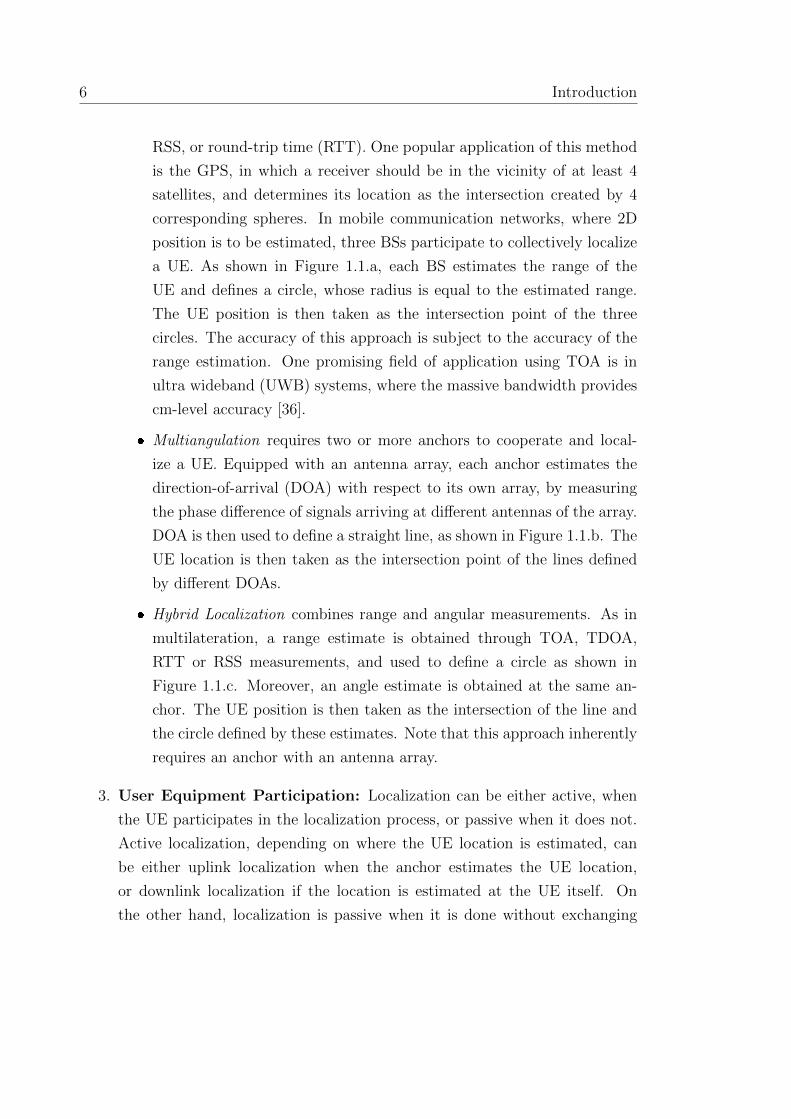
6 Introduction
RSS, or round-trip time (RTT). One popular application of this method
is the GPS, in which a receiver should be in the vicinity of at least 4
satellites, and determines its location as the intersection created by 4
corresponding spheres. In mobile communication networks, where 2D
position is to be estimated, three BSs participate to collectively localize
a UE. As shown in Figure 1.1.a, each BS estimates the range of the
UE and defines a circle, whose radius is equal to the estimated range.
The UE position is then taken as the intersection point of the three
circles. The accuracy of this approach is subject to the accuracy of the
range estimation. One promising field of application using TOA is in
ultra wideband (UWB) systems, where the massive bandwidth provides
cm-level accuracy [36].
� Multiangulation requires two or more anchors to cooperate and local-
ize a UE. Equipped with an antenna array, each anchor estimates the
direction-of-arrival (DOA) with respect to its own array, by measuring
the phase difference of signals arriving at different antennas of the array.
DOA is then used to define a straight line, as shown in Figure 1.1.b. The
UE location is then taken as the intersection point of the lines defined
by different DOAs.
� Hybrid Localization combines range and angular measurements. As in
multilateration, a range estimate is obtained through TOA, TDOA,
RTT or RSS measurements, and used to define a circle as shown in
Figure 1.1.c. Moreover, an angle estimate is obtained at the same an-
chor. The UE position is then taken as the intersection of the line and
the circle defined by these estimates. Note that this approach inherently
requires an anchor with an antenna array.
3. User Equipment Participation: Localization can be either active, when
the UE participates in the localization process, or passive when it does not.
Active localization, depending on where the UE location is estimated, can
be either uplink localization when the anchor estimates the UE location,
or downlink localization if the location is estimated at the UE itself. On
the other hand, localization is passive when it is done without exchanging

1.2 Classification of Localization Systems 7
messages. Also known as device-free localization, passive localization usually
applied to estimating the location of obstacles such as scatterers, from which
an environment map can then be created.
4. Processing Location: When more than one anchor are involved, localiza-
tion systems can be classified based on the premises where the estimation
process takes place, as centralized of distributed (cooperative). Centralized
systems are those which collect measurements at different anchors and then
the whole location estimation process takes place at a dedicated processing
center. This is the traditional approach applied in cellular networks. On the
contrary, in distributed localization, each anchor participates in the localiza-
tion process by exchanging useful information with neighboring anchors till
the unknown location is determined. This approach is widely used in WSNs.
5. User Environment: This environment can be either indoor or outdoor.
Each of these two environments has its own requirements in terms of accuracy,
algorithm complexity, and suitable infrastructure.
6. Number of Anchors: Depending on the technique used, a localization sys-
tem can comprise a single or multiple anchors. Single-anchor localization
systems can use fingerprinting, proximity or hybrid techniques. On the other
hand, by definition, multilateration and multiangulation are built with mul-
tiple anchors.
7. Number of Users: A localization system can be a single-user or multiuser.
8. User Movement: A localization system can serve a stationary, or a moving
user. In the latter case, the localization process is referred to as tracking.
9. Antenna Configuration: Single antenna localization is useful when angle
measurements are not involved, in which case an antenna array is required.
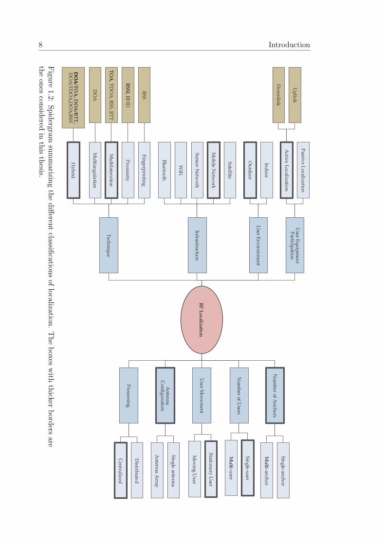
The classification of the localization systems is summarized in Figure 1.2.
8 Introduction
Nu
mb
er of An
cho
rs
Pro
cessing
An
tenn
a C
on
figu
ration
User E
qu
ipm
ent
Particip
ation
Nu
mb
er of Users
User E
nv
iron
men
t
Tech
niq
ue
Infrastru
cture
User M
ov
em
ent
Sin
gle-an
cho
r
Mu
lti-anch
or
Satellite
Mo
bile N
etwo
rk
Sen
sor N
etwo
rk
WiF
i
Blu
etoo
th
Statio
na
ry U
ser
Mo
vin
g U
ser
Fin
gerp
rintin
g
Pro
ximity
Mu
ltilateratio
n
Mu
ltiang
ula
tion
Hy
brid
Ind
oo
r
Ou
tdo
or
Sin
gle-u
ser
Mu
lti-user
Passiv
e Localizatio
n
Activ
e L
ocalizatio
n
Sin
gle an
ten
na
An
tenn
a Array
Distrib
ute
d
Cen
tralized
Up
link
Do
wn
link
RS
S
RS
SI, R
FID
TO
A, T
DO
A, R
SS
, RT
T
DO
A
DO
A/T
OA
, DO
A/R
TT
, D
OA
/TD
OA
,DO
A/R
SS
RF
Lo
calization
Figu
re1.2:
Spid
ergramsu
mm
arizing
the
diff
erent
classification
sof
localization
.T
he
box
esw
ithth
ickerb
orders
areth
eon
escon
sidered
inth
isth
esis.

1.3 Challenges Facing Localization Systems 9
1.3 Challenges Facing Localization Systems
From our discussion so far, it can be seen that localization is highly dependent on
accurate channel and transceiver models in order to take accurate measurement
of time, phase, power level, or a combination of them. However, sometimes these
models are not sufficiently accurate, which may deteriorate the expected perfor-
mance if the underlying impairments are not properly addressed. In this section,
we discuss the main challenges a localization system may face.
One of the main challenges in this context is the presence of none-line-of-sight
(NLOS) paths between the transmitter and receiver [41,42]. In many of the local-
ization methods, measurement of TOA, DOA or RSS of the line-of-sight (LOS) are
needed to establish the location of the UE. However, in a multipath environment,
the measurements may not be related to the LOS. Moreover, NLOS signals travel
longer distances than LOS, which introduces a positive range bias on the measure-
ments. Therefore, the presence of NLOS paths can cause significant performance
deterioration or even the collapse of the localization process, and thus must be
remedied to preserve the robustness. One way to deal with this issue is the “iden-
tify and mitigate”, in which a path is identified statistically to be either LOS or
NLOS, before incorporating this information in the localization process [43–47]. On
the other hand, the “identify and discard” approach cleans the signal by retaining
the information of the LOS path only [42, 48, 49]. Moreover, convex optimization
tools have also been used to estimate the UE location in the presence of NLOS
paths, without the need to identify the link status [1, 50–55].
Another challenge that usually faces localization is the tight synchronization
requirement between the anchors and the UE. TOA measurements, and the result-
ing range measurements, are only useful if the time at which the signal departed
the transmitter is known. Therefore, the clocks of the receiver and the transmit-
ter should be synchronized to guarantees a sample-rate at the receiver similar to
that at the transmitter, with no excess time offset [36, 56, 57]. Similarly, DOA
measurements are based on measurements of the signal phase of arrival [58], which
means that timing and carrier frequency offsets should be synchronized in that case.
Although communication systems are synchronized in most cases, the level of syn-
chronization is not usually high enough to suit localization. This being said, there

10 Introduction
are applications that do not require time synchronization, such as those involving
RSS and TDOA2 [36].
Systems relying on DOA estimation must be equipped with antenna arrays. For
reliable positioning using DOA, the array must have antennas with known electric
characteristics such as gain and phase. The antenna locations and inter-antenna
spacing should also be known. However, in reality the antenna electric character-
istics may vary over time, and it is hard to guarantee the array element locations
exactly as the design values. Therefore, for robust localization performance using
antenna array, a process called array calibration is sometimes necessary [59]. Com-
pensating for the gain, phase or antenna elements location errors, array calibration
is achieved using pilots of known nature transmitted from known locations [59,60].
In many localization applications, the UE to be localized is assumed to be
stationary. However, applications based on this assumption, may not work if the
user is moving in a car or a train for example. Relative motion of the receiver with
respect to the transmitter is known to introduce the Doppler effect which affects
the synchronization and consequently the localization accuracy [39]. To overcome
this issue, systems with potentially moving users observe signals over a very short
period of time, or use tracking methods, such as Kalman filter, to obtain and
predict the location of the UE [29] [38].
Finally, localization algorithms, especially those involving antenna arrays and
3D localization, can be very demanding in terms of device processing resources and
physical size. Thus, most algorithms are traditionally designed to be executed at
the anchors that have superior computation powers, or resort to a design trade-off
between performance and complexity. Nevertheless, with the smart devices having
a growing processing power, more complexity is being pushed in the UE nowadays,
especially in device-to-device communication paradigms [61].
1.4 5G: Localization Opportunities and Challenges
Mobile technology is one of the most successful ambient technologies. This is why,
recently there has been a significant increase in the bandwidth requirement. Not
2In TDOA, synchronization between the UE and BSs is not required. However, the differentBSs must be synchronized, which is easy to achieve [36].

1.4 5G: Localization Opportunities and Challenges 11
only the number of users increased but also the number of devices (phone, tablets,
smart watches,... etc.) per user and the data volume per device have also im-
mensely increased. While internet access from a mobile device was initially for
browsing and other low-to-medium size data usages, nowadays with the ubiquity
of social networks and video-on-demand services, users expect to be able to stream
network-demanding contents such as ultra high-definition movies, and video calls
with high quality. Advanced techniques to optimize the latest mobile commu-
nication have almost been depleted, whether using orthogonal frequency-division
multiplexing (OFDM), multiple-input multiple-output (MIMO), multi-user diver-
sity, link adaptation, turbo code, or hybrid automatic repeat request (HARQ) [62].
Therefore, a move to a new generation (5G) is necessary, and would involve radical
adoption of disruptive technologies including: massive MIMO and mmWave [61].
MmWave 5G systems are characterized by frequencies of 30–300 GHz. At these
high frequencies, the path loss becomes more significant than in the sub-6 GHz
bands [62–65]. Therefore, the use of dedicated techniques to provide sufficient gain
will be necessary to counter-act the increasing path loss. By virtue of mmWave
tiny wavelengths, a large number of antennas can be packed in a small area. Thus,
beamforming at the transmitter and receiver will be a natural techniques to use.
Moreover, mmWave channels have no diffraction, are sensitive to blockage, and
enjoy a low scattering/reflective nature, causing the channel to be sparse, with
the number of paths limited to just a few [64, 66]. The small number of paths
and the use of beamforming mean that mmWave communication is dominated by
LOS and limited NLOS communication, hence, can be considered quasi-optical
[67]. Furthermore, moving to higher carrier frequencies in bands that are barely
occupied, mmWave will employ a very large bandwidth supporting 1 Gbps data
rate, and providing reduced latency [62].
From a localization point-of-view, the large number of antennas and the large
bandwidth facilitate estimating the DOA, DOD and TOA with a high degree of
accuracy, leading to the following implications:
1. UE position Estimation using a single anchor can potentially be very accurate.
2. The low-error estimate of location will unlock a wide range of location-aware
applications, including vehicle-to-vehicle and vehicle-to-everything commu-
12 Introduction
nications [30, 31], intelligent health systems [68], environment mapping [69],
targeted content delivery [70], and public safety applications [32].
3. Due to the highly directive nature of mmWave channels, incorporating lo-
calization in the network design and optimization will be an indispensable
feature [26]. In fact, 5G will be the first generation of mobile communication
to do that [26], with many research nowadays investigating the possibilities.
For example, it has been shown that location-awareness can boost the network
performance if pilots are assigned based on the user location [34]. Moreover,
location determination assists in more efficient beamforming schemes [33,71].
Furthermore, spatial-devision multiple access can be better optimized when
the user location is known [35].
High performance localization schemes in 5G, will not be possible without ef-
ficient beamforming techniques. However, there are mainly three challenges in 5G
mmWave beamforming. Firstly, due to the high directivity of mmWave channels,
beam alignment of the UE and BS in the initial access (IA) to the network(network
discovery phase) becomes an important issue to address [64,72]. On the other hand,
analog-to-digital converters are known to be highly power dissipating. Therefore,
it will be infeasible to employ all-digital beamforming, especially with the large
number of antennas. Towards that, analog beamforming, or hybrid beamforming
architecture have been proposed for 5G mmWave devices [64]. Moreover, beam-
forming at UE is highly sensitive to the device orientation, since steering the device
away from the BS, may point beams towards directions not useful for localization.
In addition to the challenges of a classical a localization system discussed in Sec-
tion 1.3, to meet accuracy requirements, 5G localization systems need to address
the high computational and processing complexity stemming from the large num-
ber of antennas and large bandwidth. Handover and location information fusion
from different localization methods will also be a challenge [26]. Finally, since a UE
is usually associated with one person, the abundance of location-aware communi-
cation will raise legal issues regarding privacy as it would reveal the user location,
speed, and means of transport [73].
Finally, it is worth mentioning that during a late phase of writing this thesis,
the first 5G standard was approved by 3GPP in December 2017. Under the New

1.5 Thesis Scope and Overview 13
Radio (NR) series, the 5G NR Release 15 [74] defines actual baseline physical layer
components, system specifications and radio access functionalities up to 52.5 GHz.
As the work on 5G localization incorporated in this thesis started in 2015, when 5G
was in its infancy, reflecting this standard in the current thesis was not possible.
1.5 Thesis Scope and Overview
The next generation of mobile communication systems (5G) is expected to provide
an excellent platform of a wide range applications of location-aware communica-
tion. In this context, localization can be seen as a key enabler of such systems.
Therefore, it is imperative to study localization in the context of 5G mmWave sys-
tems. 3Although localization techniques have been an actively-researched topic over
the past decades, there are still many open problems which researchers have not
solved or understood yet. With focus on outdoor mobile localization, this thesis
contributes to the field’s aggregated knowledge by providing applied and funda-
mental research results that address open areas of localization with more focus on
5G mmWave systems. The thesis studies NLOS localization in various outdoor
environments of conventional communication systems (sub-6 GHz). Subsequently,
focusing on 5G mmWave systems, which is still in its infancy, the thesis explores
fundamental performance bounds of location estimation, and provides a deep un-
derstanding of the factors that together affect these bounds, and shows how this
understanding can be exploited to better design 5G communication systems and
localization algorithms.
The main contribution this thesis provides is a fundamental understanding of
how 5G mmWave technology can enable extremely accurate localization. By study-
ing theoretical performance bounds, we aim to provide insights on the feasibility
and the factors that need to be considered when designing 5G localization systems
in order to achieve the required high location accuracy. The localization systems
considered in this thesis follow the classifications in Figure 1.2, highlighted with
thicker box borders. That is, we consider single-stationary-user active outdoor lo-
3It is commonly understood that the first commercial deployments of 5G technology will focuson centimeter-wave technology. However, we focus on 5G systems that are related to the highlyanticipated mmWave systems

14 Introduction
calization for mobile communications networks using multilateration and hybrid
approaches.
Research Questions
The research presented in this thesis seeks to address the following research ques-
tions:
1. In sub-6 GHz, given an environment with a given scattering richness, what
is the best expected performance? How can we exploit the NLOS propaga-
tion models to better design localization algorithm with performance that ap-
proaches the best performance?
2. Focusing on 5G mmWave communications systems, and considering the ini-
tial network access problem, how can we use a blind beamforming technique
that provides the UE with a reasonable access to the network?
3. Beyond the IA phase, is it better to perform localization at the BS (Uplink)
or at the UE (downlink)? How does the unique mmWave channel features
impact this performance? What is the best positioning performance that can
be achieved?
4. What are the system parameters that need to be tuned in order to boost the
performance of 5G mmWave localization? How do these parameters affect
the performance?
5. Building on the results of questions 3 and 4, how can we account for synchro-
nization issues in mmWave?
Thesis Overview
The remainder of this thesis is organized as follows:
� Chapter 2 provides the background necessary to understand the thesis. This
includes a brief revision of relevant notions from array signal processing, a
review of some concepts of estimation theory, and an overview with some
example on how to compute the Cramer-Rao lower bound (CRLB). CRLB is

1.5 Thesis Scope and Overview 15
a performance metric widely-used to judge and benchmark estimation prob-
lems, of which localization is one.
� Chapter 3 proposes a trilateration-based localization scheme applicable in
conventional cellular systems and accounts for different NLOS environments.
Towards that, we devise an unbiased ranging method that is based on a
distance-dependent bias model. Then, incorporating range estimate from 3
BSs, we localize UE. We perform an error analysis and compare it with the
distance CRLB that is obtained using numerical statistical methods. We do
that for mixed LOS/NLOS scenarios in four environments, ranging from bad
urban environment to rural environment.
� Chapter 4 focuses on the initial access problem in 5G mmWave networks,
when no channel-side information is available at the UE that attempts to gain
network access. In this regard, the chapter investigates two blind beamform-
ing schemes, referred to as random-phase beamforming (RPBF) and direc-
tional beamforming (DBF). Since the subsequent step to initial access would
be channel estimation, we compare the performance of DBF and RPBF in
terms of CRLB of the channel parameters. We show that under the consid-
ered scenarios, RPBF is more appropriate.
� Chapter 5 considers the 3D positioning error bound of 5G mmWave systems
in multipath propagation, both uplink and downlink, beyond the initial access
phase. It analyzes the impact of system parameters, and the interaction
between different paths in terms of information gain. It also explores the
role of reflectors, and scatterers on the localization limits. The problem
of jointly estimating the UE location and orientation is considered, since
beamforming at the UE in mmWave systems (hence, systems performance)
depends on the UE orientation. The results in this chapter imply that uplink
and downlink are not equivalent, and that NLOS paths assist localization
in general. Moreover, we show that mmWave systems can provide a sub-
meter position and sub-degree orientation errors, if the systems parameters
are tuned appropriately.
� Chapter 6 extends the results in Chapter 5 by focusing on LOS scenarios,

16 Introduction
and accounting for the time-offset bias issue. It proposes two-way localiza-
tion protocols, distributed and centralized and compares them in terms of
the uplink and downlink position error bounds in the presence of receive
beamforming and spatially correlated noise. We deduce that the central-
ized protocol outperforms the distributed protocol, with the cost of requiring
coarse synchronization.
� Chapter 7 provides a summary of the important results of the thesis and
sheds some light on related future research directions.
Chapter 2
Background Concepts
Overview: The reader of this thesis encounters many concepts of array signal pro-
cessing and classical estimation theory. Therefore, it is meaningful to cover these
concepts in this Chapter. The Chapter starts by giving an overview on the field of
array signal processing, where the coordinate system is defined, and the concept of
array manifold vector is introduced. Subsequently, analog beamforming and the re-
sulting channel model useful in 5G mmWave are described. In the second part of the
Chapter, the basics of estimation theory are covered, and the measurement model is
discussed. The assessment of the estimation performance is highlighted thereafter.
The concepts of Cramer-Rao Lower Bound (CRLB) and Fisher Information Ma-
trix (FIM) are frequently encountered throughout this thesis. Therefore, they are
introduced later in this Chapter. Moreover, we observe one variable sometimes,
but are interested in another, which is a function of the observed one. Towards
that, we discuss the transformation of parameters. To conclude this Chapter, the
equivalent FIM (EFIM) is briefed at the end. To make the concepts in this chapter
clearer, some relevant examples were designed and included herein. We stress that
this Chapter is not to meant to be all-inclusive, and that only background relevant
to the thesis is provided. However, we provide highlights to guide the reader to
other resources, should more comprehensive background be necessary.
17

18 Background Concepts
2.1 Background on Array Signal Processing
As the name suggests, array signal processing is a branch of signal processing that
focuses on signals received by a group of sensors. These sensors are spatially “ar-
rayed” by a specific geometry that affects the behavior of the sensors ensemble. In
the context of this thesis, the sensors we are focusing on are antennas, as traducers
of electromagnetic waves into electrical signals. Since the signal arrives at the array
elements in delayed versions, the signal received at the output of an antenna array
carries two-part information: spatial and temporal. Employing this spatiotempo-
ral information, array signal processing addresses four problems [75]. Firstly, the
detection problem is concerned with estimating the number of emitting sources.
Secondly, the DOA estimation problem, known as direction finding, employs the
spatial information of the received signal to infer information on the direction from
which the signal is impinging on the array. Then in combination with TOA es-
timation, the location of the transmitter can therefore be determined. Moreover,
the reception problem addresses the design of beamforming schemes to extract the
desired signal and cancel the interference. Finally, environment mapping seeks to
create a map of the surrounding environment based on the received signal features
such as signal density based on the spatial coordinates. In this thesis, we focus
on the location estimation bounds, and beamforming. Thus, only array process-
ing basics that are related to these two concepts are introduced in this chapter.
However, a reader interested in comprehensive background on array processing is
referred to the books [58, 75–79], which cover a wide range of topics with varying
levels of complexity, while [80] provides a good overview on the topic.
2.1.1 Array Manifold Vector
Firstly, we need to understand how the antenna array behaves as an ensemble.
Towards that, the array manifold vector, provides us with this understanding [58,
75]. It is reasonable to expect the array manifold vector to depend on the array
geometry. Therefore, we start by defining the standard spherical coordinate system,
used in this thesis. From Figure 2.1, for 0 ≤ θ ≤ π, 0 ≤ φ < 2π, and % ≥ 0, we

2.1 Background on Array Signal Processing 19
θ
%
φ
(x, y, z)
x
y
z
Figure 2.1: Spherical coordinate system.
can write
x = % sin θ cosφ, (2.1a)
y = % sin θ sinφ, (2.1b)
z = % cos θ. (2.1c)
Based on this notation, we define a unit vector pointing towards (x, y, z) as u ,
[sin θ cosφ, sin θ sinφ, cos θ]T, from which the wavenumber vector can be defined as
k(θ, φ) ,2π
λu =
2π
λ[sin θ cosφ, sin θ sinφ, cos θ]T, (2.2)
where λ = c/fc is the wavelength, c is the propagation speed, and fc is the carrier
frequency. Furthermore, considering an array of NR antennas, denote the location
of the nth antenna, 1 ≤ n ≤ NR, in Cartesian coordinates by un = [xn, yn, zn]T ∈R3. The the antenna location matrix is given by
∆R = [u1,u2, · · · ,uNR] ∈ R3×NR . (2.3)
Consequently, the array manifold vector is defined by [58,75]
aR(θ, φ) , g(θ, φ)� exp(−j∆T
Rk(θ, φ)), (2.4)
20 Background Concepts
where � denotes the Hadamard product, and g(θ, φ) ∈ CNR is a vector specifying
the directional gain and phase of each antenna element. In our work, as the case
with most literature, we will assume that the antennas radiation pattern is isotropic.
That is,
aR(θ, φ) =1√NR
exp(−j∆T
Rk(θ, φ)), (2.5)
Note that we use√NR to normalize aR(θ, φ), such that aT
A(θ, φ)aR(θ, φ) = 1.
Moreover, observe that aR(θ, φ), encapsulates the phase difference of arrival at
each antenna. Finally, note that usually the term “array manifold vector” is used
as a unified term that applies to both transmitter and receiver. However, “array
response vector” is the popular used with receiving arrays, while “array steering
vector” is the one used with transmitting arrays. After all, these three terms
describe the vector defined in (2.5).
In the following, we show how to obtain the array manifold vector for example
geometries.
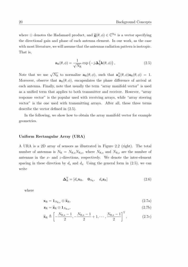
Uniform Rectangular Array (URA)
A URA is a 2D array of sensors as illustrated in Figure 2.2 (right). The total
number of antennas is NR = NR,xNR,z, where NR,x and NR,z are the number of
antennas in the x- and z-directions, respectively. We denote the inter-element
spacing in these direction by dx and dz. Using the general form in (2.5), we can
write
∆TR = [dxxR, 0NR
, dzzR] (2.6)
where
xR = 1NR,z⊗ xR, (2.7a)
zR = zR ⊗ 1NR,x, (2.7b)
xR ,
[−NR,x − 1
2,−NR,x − 1
2+ 1, · · · , NR,x − 1
2
]T
, (2.7c)

2.1 Background on Array Signal Processing 21
x
z
x
z
dx
dx
dz
Figure 2.2: Left: ULA with 9 antennas and dx inter-element spacing. When dx =λ/2 it is called SLA. Right: URA of 45 antennas, consisting of 9 ULAs, each with5 antennas and dx inter-element spacing. Spacing between adjacent arrays is dz.
zR ,
[−NR,z − 1
2,−NR,z − 1
2+ 1, · · · , NR,z − 1
2
]T
. (2.7d)
and ⊗ denotes the Kronecker product. Consequently, we obtain
aR(θ, φ) =1√NR
exp
(−j 2π
λ(dx sin θ cosφ xR + dz cosφ zR)
). (2.8)
Note that when dx = dz = λ/2, and NR,x = NR,z, the array is called standard
square array (SSA).
Uniform Linear Array (ULA)
A ULA is an 1-dimensional array of sensor with equispaced antennas as illustrated
in Figure 2.2 (left). It is easy to see that a ULA is a special case URA with
NR,z = 1. Therefore,
xR = xR, zR = 0NR, θ =
π
2. (2.9)
22 Background Concepts
Thus, the array response vector is given by
aR(φ) ,1√NR
exp
(−j 2πdx
λcosφ xR
), (2.10)
Note that when dx = λ/2, the ULA is called standard linear array (SLA).
2.1.2 Analog Beamforming
One of the great advantages of array signal processing is enabling us to focus the
transmission or reception on some specific areas by steering the beams electron-
ically, rather than mechanically as in traditional radar systems. We can achieve
that through a process called beamforming, whereby we scale the signal on each
antenna by some complex weight to alter its magnitude and phase, so that the
overall antenna gain is higher in the desired areas than in the other areas [76]. In
mmWave systems, analog beamforming will be implemented using phase-shifters
only. Therefore, in this thesis, we restrict our discussion on beamforming only to
analog beamforming with constant magnitude but varying phase.
The simplest form of beamforming is when the antennas are uniformly weighted.
Considering a URA lying the xz-plane as shown in Figure 2.2, under this beam-
forming scheme, the radiation pattern of the beam points towards θ = φ = 90◦.
Similarly, in the case of a ULA along the x-axis, it points towards the broadside
direction, φ = 90◦ [58]. An example radiation pattern of a 12-antenna ULA is
shown in Figure 2.3. This radiation pattern is often called an array factor, which
is the radiation pattern of an “unsteered” beam [58].
Mathematically, for any beamforming vector f , the beam gain in the direction
(θ, φ) is given [76]
G(θ, φ)[dB] = 20 log10
(‖fHa(θ, φ)‖‖f‖
). (2.11)
Consider a transmitting array with NT antennas, and assume that we want to
transmit a beam towards a direction (θ0, φ0). In that case, we can design f to be
f(θ0, φ0) = aT(θ0, φ0) ,1√NT
exp(−j∆T
Tk(θ0, φ0)). (2.12)

2.1 Background on Array Signal Processing 23
0 20 40 60 80 100 120 140 160 180−50
−40
−30
−20
−10
0
φ
Array
Gain
Figure 2.3: An array factor of a 12-antenna standard ULA.
Figure 2.4: Radiation Pattern of a 12-antenna ULA, steered to 60◦, and 125◦.
Throughout this thesis, we will refer to this type of beamforming as directional
beamforming. The array factor of the 12-antenna ULA shown in Figure 2.3 is
replotted in polar form in Figure 2.4 (blue), steered to the directions 60◦, and 125◦.
24 Background Concepts
splitters(t) y(t)
f1
f2
...
fNT
w∗1
w∗2
...
w∗NR
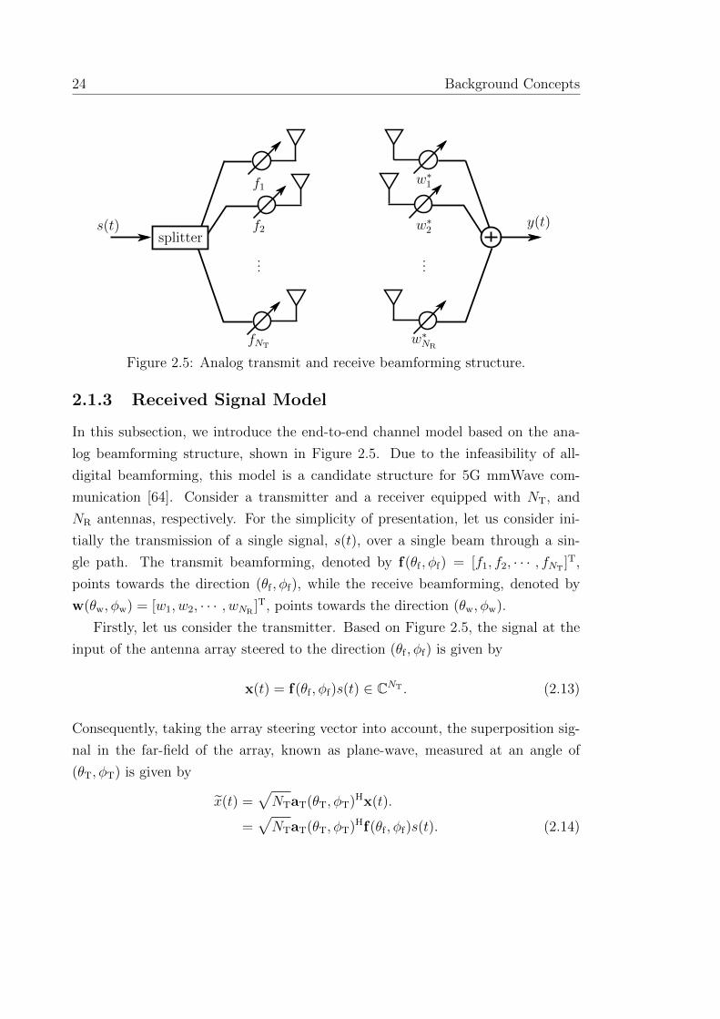
Figure 2.5: Analog transmit and receive beamforming structure.
2.1.3 Received Signal Model
In this subsection, we introduce the end-to-end channel model based on the ana-
log beamforming structure, shown in Figure 2.5. Due to the infeasibility of all-
digital beamforming, this model is a candidate structure for 5G mmWave com-
munication [64]. Consider a transmitter and a receiver equipped with NT, and
NR antennas, respectively. For the simplicity of presentation, let us consider ini-
tially the transmission of a single signal, s(t), over a single beam through a sin-
gle path. The transmit beamforming, denoted by f(θf , φf) = [f1, f2, · · · , fNT]T,
points towards the direction (θf , φf), while the receive beamforming, denoted by
w(θw, φw) = [w1, w2, · · · , wNR]T, points towards the direction (θw, φw).
Firstly, let us consider the transmitter. Based on Figure 2.5, the signal at the
input of the antenna array steered to the direction (θf , φf) is given by
x(t) = f(θf , φf)s(t) ∈ CNT . (2.13)
Consequently, taking the array steering vector into account, the superposition sig-
nal in the far-field of the array, known as plane-wave, measured at an angle of
(θT, φT) is given by
x(t) =√NTaT(θT, φT)Hx(t).
=√NTaT(θT, φT)Hf(θf , φf)s(t). (2.14)

2.1 Background on Array Signal Processing 25
x(t) arrives at the receiver after some propagation delay, τ . Thus, ignoring the
path gain and the receiver noise, for the time-being, the signal received via the
direction (θR, φR) at the output of the receive array is modeled by
r0(t) =√NRaR(θR, φR)x(t− τ),
=√NTNRaR(θR, φR)aT(θT, φT)Hf(θf , φf)s(t− τ). (2.15)
Adding the channel gain, β, and the receiver noise, n(t) to the model yields,
r(t) =√NTNRβaR(θR, φR)aT(θT, φT)Hf(θf , φf)s(t− τ) + n(t) ∈ CNR . (2.16)
Defining Hs ,√NTNRβaR(θR, φR)aT(θT, φT)H. Subsequently, the signal processed
by a receive beamformer pointing towards (θw, φw) is then given by
ys(t) = wH(θw, φw)r(t),
= wH(θw, φw)Hsf(θf , φf)s(t− τ) + wH(θw, φw)n(t) ∈ CNR . (2.17)
Finally, with similar steps, we can extend the single-path single-beam model in
(2.17) to NB beams and M paths. The resulting receive signal is then given by
y(t) = WH
M∑
m=1
HmFs(t− τm) + WHn(t) ∈ CNB , (2.18)
where
� W , [w(θw,1, φw,1),w(θw,2, φw,2), · · · ,w(θw,NB, φw,NB
)] , is the receive beam-
forming matrix, stacking the receive beamformers. The receive angles are
dropped for concise presentation.
� F , [f(θf,1, φf,1), f(θf,2, φf,2), · · · , f(θf,NB, φf,NB
)] , is the transmit beamforming
matrix, stacking transmit beamformers. The transmit angles are dropped for
concise presentation too.
� Hm =√NTNRβmaR(θR,m, φR,m)aT(θT,m, φT,m)H, the channel excluding the
propagation delay, where βm is the mth path gain, (θR,m, φR,m) is the mth
DOA, and (θT,m, φT,m) is the mth DOD.
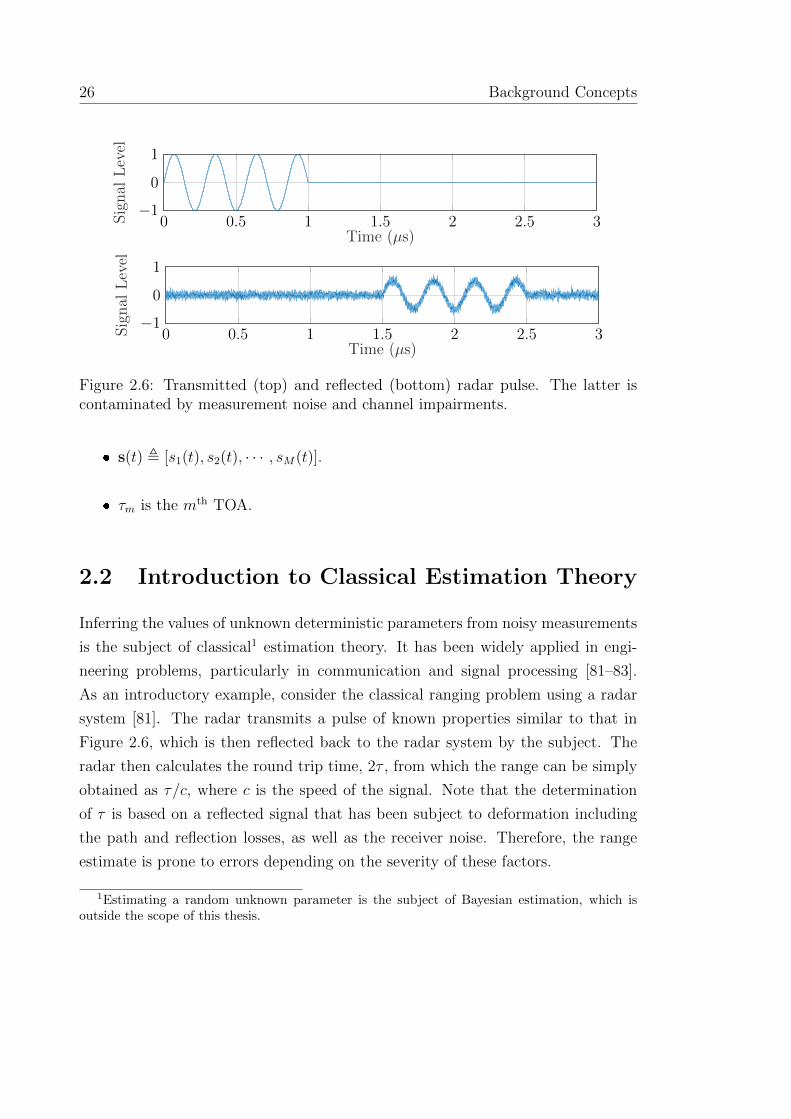
26 Background Concepts
0 0.5 1 1.5 2 2.5 3−1
0
1
Time (µs)
Signal
Level
0 0.5 1 1.5 2 2.5 3−1
0
1
Time (µs)
Signal
Level
Figure 2.6: Transmitted (top) and reflected (bottom) radar pulse. The latter iscontaminated by measurement noise and channel impairments.
� s(t) , [s1(t), s2(t), · · · , sM(t)].
� τm is the mth TOA.
2.2 Introduction to Classical Estimation Theory
Inferring the values of unknown deterministic parameters from noisy measurements
is the subject of classical1 estimation theory. It has been widely applied in engi-
neering problems, particularly in communication and signal processing [81–83].
As an introductory example, consider the classical ranging problem using a radar
system [81]. The radar transmits a pulse of known properties similar to that in
Figure 2.6, which is then reflected back to the radar system by the subject. The
radar then calculates the round trip time, 2τ , from which the range can be simply
obtained as τ/c, where c is the speed of the signal. Note that the determination
of τ is based on a reflected signal that has been subject to deformation including
the path and reflection losses, as well as the receiver noise. Therefore, the range
estimate is prone to errors depending on the severity of these factors.
1Estimating a random unknown parameter is the subject of Bayesian estimation, which isoutside the scope of this thesis.

2.2 Introduction to Classical Estimation Theory 27
2.2.1 Measurement Model
Consider the problem of estimating a vector ofNv parameters, ϕ , [ϕ1, ϕ2, · · · , ϕNv ]T,
using NR observation channels, r(t) , [r1(t), r2(t), · · · , rNR(t)]T, such that
r(t) = µϕ(t) + n(t), 0 ≤ t ≤ To. (2.19)
In (2.19), µϕ(t) is a deterministic vector function of the unknown parameter vector,
n(t) ∼ CN (0,Σn) is the measurement noise vector, Σn is the noise covariance
matrix, and To is the observation interval.
The estimator of ϕ is given by some vector function g(.) as ϕ = g (r(t)). Note
that r(t) is observed in the presence of noise. Therefore, ϕ is a random vector,
and r(t) is a random process whose distribution depends on the noise probability
density function (PDF). In most estimation theory applications, the measurements
are generally modeled by Gaussian processes such that the PDF of r as a function
of ϕ is
fr(r;ϕ) =1
det(2πΣn)12
e−12
(µϕ−r)HΣ−1n (µϕ−r), (2.20)
Recall that it is very common to assume that observations are contaminated by
zero-mean and independent and identically distributed Gaussian noise, in which
case Σn = N0INR, where N0 is the noise power spectral density (PSD), and INR
is
the NR-dimensional identity matrix.
Based on this PDF, the issue becomes: how can we design a “good” estimator,
ϕ? And, what is a “good” estimator? In the following, we answer these questions.
2.2.2 Estimation Performance
As an optimality criterion to assess the estimator performance, we start by the
estimator mean-square error (MSE) denoted by ρ, and defined as,
ρ(ϕ) , E{
(ϕ−ϕ)2} =
E{
(ϕ1 − ϕ1)2}...
E{
(ϕNv − ϕNv)2}
, (2.21)
28 Background Concepts
where E {·} is the expectation operator. Without loss of generality, consider the
MSE of ϕ1, and write [81] as
ρ(ϕ1) = E{
(ϕ1 − ϕ1)2} , (2.22a)
= E{
(ϕ1 − E {ϕ1}+ E {ϕ1} − ϕ1)2}, (2.22b)
= E{
(ϕ1 − E {ϕ1})2}
+ (E {ϕ1} − ϕ1)2 . (2.22c)
This means that the estimator error has two components: a variance, σ2ϕ1,
E{
(ϕ1 − E {ϕ1})2}, and a bias, bϕ1 , (E {ϕ1} − ϕ1)2. Any good estimator should
provide an estimate of the variable that is equal to the said variable on the average.
Such an estimator is called unbiased estimator, and is characterized by
ϕ1 = E {ϕ1} ⇒ bϕ1 = 0. (2.23)
Consequently, in the absence of estimation bias, the best estimator is the one
that provides the least variance. This minimum variance is known as Cramer-Rao
lower bound (CRLB), and the estimator that attains the CRLB is called minimum
variance unbiased estimator (MVUE). Unfortunately, the MVUE does not always
exist, or may not be practically possible [81]. Moreover, a closed-form procedure
to compute the MVUE estimator does not exist. The computation of CRLB is
discussed in more details in the following section.
2.2.3 Cramer-Rao lower bound (CRLB)
In the context of parameter estimation, CLRB is a useful tool that serves as a feasi-
bility study on whether a given technology can meet some performance requirement
or not. Being a lower bound, it can also be used to benchmark the performance
of new estimators. Moreover, it can be used in investigating the impact of differ-
ent system parameters on the overall performance of an estimator. Finally, CRLB
may provide means to compute a MVUE. The use of CRLB in benchmarking is
applied in Chapter 3, while its use for feasibility studies, and investigating system
parameters impact is applied in Chapters 4, 5, and 6.
2.2 Introduction to Classical Estimation Theory 29
Assuming that the PDF fr(r;ϕ) satisfies the regularity condition
E{∂ ln fr(r;ϕ)
∂ϕ
}= 0Nv , (2.24)
then the variance of any unbiased estimator of ϕ, is computed from the information
inequality given by [81,83]
σ2ϕ1
...
σ2ϕNv
≥ diag
(J−1ϕ
), (2.25)
where Jϕ is the Fisher Information Matrix (FIM), whose elements are given by
[Jϕ]u,v , E{∂ ln fr(r;ϕ)
∂ϕu
∂ ln fr(r;ϕ)
∂ϕv
}, 1 ≤ u, v ≤ Nv (2.26)
The CRLB is then related to the FIM by
CRLB(ϕ) ,
CRLB(ϕ1)...
CRLB(ϕNv)
= diag
(J−1ϕ
). (2.27)
We now consider the most used case of Gaussian distribution. It is easy to see
from (2.20) that the regularity condition is satisfied, and that the CRLB is defined
for the Gaussian PDFs. For the vector Gaussian PDF given in (2.20), using (2.26),
it can be shown the FIM entries are given by [81–83]
[Jϕ]u,v ,∫ To
0
<{∂µH
ϕ(t)
∂ϕuΣn−1∂µϕ(t)
∂ϕv
}dt, 1 ≤ u, v ≤ Nv (2.28)
For the widely-used case of i.i.d Gaussian noise,
[Jϕ]u,v ,1
N0
∫ To
0
<{∂µH
ϕ(t)
∂ϕu
∂µϕ(t)
∂ϕv
}dt, 1 ≤ u, v ≤ Nv (2.29)
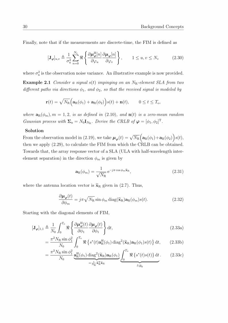
30 Background Concepts
Finally, note that if the measurements are discrete-time, the FIM is defined as
[Jϕ]u,v ,1
σ2n
Ns∑
n=0
<{∂µH
ϕ[n]
∂ϕu
∂µϕ[n]
∂ϕv
}, 1 ≤ u, v ≤ Nv (2.30)
where σ2n is the observation noise variance. An illustrative example is now provided.
Example 2.1 Consider a signal s(t) impinging on an NR-element SLA from two
different paths via directions φ1, and φ2, so that the received signal is modeled by
r(t) =√NR
(aR(φ1) + aR(φ2)
)s(t) + n(t), 0 ≤ t ≤ To,
where aR(φm),m = 1, 2, is as defined in (2.10), and n(t) is a zero-mean random
Gaussian process with Σn = N0INR. Derive the CRLB of ϕ = [φ1, φ2]T.
Solution
From the observation model in (2.19), we take µϕ(t) =√NR
(aR(φ1)+aR(φ2)
)s(t),
then we apply (2.29), to calculate the FIM from which the CRLB can be obtained.
Towards that, the array response vector of a SLA (ULA with half-wavelength inter-
element separation) in the direction φm is given by
aR(φm) =1√NR
e−jπ cosφmxR , (2.31)
where the antenna location vector is xR given in (2.7). Thus,
∂µϕ(t)
∂φm= jπ
√NR sinφm diag(xR)aR(φm)s(t). (2.32)
Starting with the diagonal elements of FIM,
[Jϕ]1,1 ,1
N0
∫ To
0
<{∂µH
ϕ(t)
∂φ1
∂µϕ(t)
∂φ1
}dt, (2.33a)
=π2NR sinφ2
1
N0
∫ To
0
<{s∗(t)aH
R(φ1) diag2(xR)aR(φ1)s(t)}
dt, (2.33b)
=π2NR sinφ2
1
N0
aHR(φ1) diag2(xR)aR(φ1)︸ ︷︷ ︸
= 1NR
xTRxR
∫ To
0
<{s∗(t)s(t)} dt
︸ ︷︷ ︸,R0
. (2.33c)
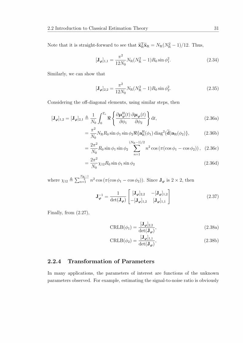
2.2 Introduction to Classical Estimation Theory 31
Note that it is straight-forward to see that xTRxR = NR(N2
R − 1)/12. Thus,
[Jϕ]1,1 =π2
12N0
NR(N2R − 1)R0 sinφ2
1. (2.34)
Similarly, we can show that
[Jϕ]2,2 =π2
12N0
NR(N2R − 1)R0 sinφ2
2. (2.35)
Considering the off-diagonal elements, using similar steps, then
[Jϕ]1,2 = [Jϕ]2,1 ,1
N0
∫ To
0
<{∂µH
ϕ(t)
∂φ1
∂µϕ(t)
∂φ2
}dt, (2.36a)
=π2
N0
NRR0 sinφ1 sinφ2<{aHR(φ1) diag2(d)aR(φ2)}, (2.36b)
=2π2
N0
R0 sinφ1 sinφ2
(NR−1)/2∑
n=1
n2 cos (π(cosφ1 − cosφ2)) , (2.36c)
=2π2
N0
χ12R0 sinφ1 sinφ2 (2.36d)
where χ12 ,∑NR−1
2n=1 n2 cos (π(cosφ1 − cosφ2)). Since Jϕ is 2× 2, then
J−1ϕ =
1
det(Jϕ)
[[Jϕ]2,2 −[Jϕ]1,2
−[Jϕ]1,2 [Jϕ]1,1
](2.37)
Finally, from (2.27),
CRLB(φ1) =[Jϕ]2,2
det(Jϕ), (2.38a)
CRLB(φ2) =[Jϕ]1,1
det(Jϕ), (2.38b)
2.2.4 Transformation of Parameters
In many applications, the parameters of interest are functions of the unknown
parameters observed. For example, estimating the signal-to-noise ratio is obviously
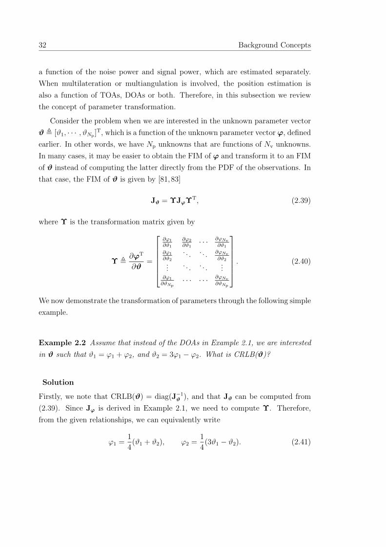
32 Background Concepts
a function of the noise power and signal power, which are estimated separately.
When multilateration or multiangulation is involved, the position estimation is
also a function of TOAs, DOAs or both. Therefore, in this subsection we review
the concept of parameter transformation.
Consider the problem when we are interested in the unknown parameter vector
ϑ , [ϑ1, · · · , ϑNp ]T, which is a function of the unknown parameter vector ϕ, defined
earlier. In other words, we have Np unknowns that are functions of Nv unknowns.
In many cases, it may be easier to obtain the FIM of ϕ and transform it to an FIM
of ϑ instead of computing the latter directly from the PDF of the observations. In
that case, the FIM of ϑ is given by [81,83]
Jϑ = ΥJϕΥT, (2.39)
where Υ is the transformation matrix given by
Υ ,∂ϕT
∂ϑ=
∂ϕ1
∂ϑ1
∂ϕ2
∂ϑ1· · · ∂ϕNv
∂ϑ1
∂ϕ1
∂ϑ2
. . . . . . ∂ϕNv
∂ϑ2...
. . . . . ....
∂ϕ1
∂ϑNp· · · · · · ∂ϕNv
∂ϑNp
. (2.40)
We now demonstrate the transformation of parameters through the following simple
example.
Example 2.2 Assume that instead of the DOAs in Example 2.1, we are interested
in ϑ such that ϑ1 = ϕ1 + ϕ2, and ϑ2 = 3ϕ1 − ϕ2. What is CRLB(ϑ)?
Solution
Firstly, we note that CRLB(ϑ) = diag(J−1ϑ ), and that Jϑ can be computed from
(2.39). Since Jϕ is derived in Example 2.1, we need to compute Υ. Therefore,
from the given relationships, we can equivalently write
ϕ1 =1
4(ϑ1 + ϑ2), ϕ2 =
1
4(3ϑ1 − ϑ2). (2.41)

2.2 Introduction to Classical Estimation Theory 33
Consequently, it follows that
Υ =1
4
[1 3
1 −1
]. (2.42)
Therefore, from (2.34), (2.35), and (2.36), it can be shown that
Jϑ =π2
16N0
[1 3
1 −1
][NR
12(N2
R − 1) sin2 ϕ1 χ12 sinϕ1 sinϕ2
χ12 sinϕ1 sinϕ2NR
12(N2
R − 1) sin2 ϕ2
][1 1
3 −1
], (2.43)
2.2.5 Equivalent Fisher Information Matrix (EFIM)
Although FIM helps us understand the interaction between different parameters,
sometimes we need to focus on a subset of the unknown parameters and study it
isolatedly. In that context, we can use the concept of equivalent FIM (EFIM) of
that parameter for our investigation [84,85].
Definition 2.1 Given a parameter vector ϕ , [ϕT1 ,ϕ
T2 ]T with corresponding FIM
Jϕ =
[J11 J12
JT12 J22
], (2.44)
Then, the EFIM of ϕ1 is given by
Jeϕ1
= J11 − J12J−122 JT
12. (2.45)
The form in (2.45) is the well-known Schur’s Complement. The first term of (2.45)
is the information content related to ϕ1, in the absence of ϕ2. Moreover, based on
the fact that information is always positive, it is interesting to see that the second
term in (2.45) is negative. This means that when we need to estimate another
parameter jointly with ϕ1, the net information at the estimator is reduced.
Example 2.3 Write the expressions in (2.38) in terms of the EFIM.
Solution

34 Background Concepts
We start by writing the determinant as:
det(Jϕ) = [Jϕ]1,1[Jϕ]2,2 − [Jϕ]21,2. (2.46)
Consequently, it is straight forward to see that
CRLB(φ1) =[Jϕ]2,2
[Jϕ]1,1[Jϕ]2,2 − [Jϕ]21,2=
1
[Jϕ]1,1 − [Jϕ]−12,2[Jϕ]21,2
=1
[Jϕ]e1,1, (2.47a)
CRLB(φ2) =[Jϕ]1,1
[Jϕ]1,1[Jϕ]2,2 − [Jϕ]21,2=
1
[Jϕ]2,2 − [Jϕ]−11,1[Jϕ]21,2
=1
[Jϕ]e2,2. (2.47b)
We can conclude from (2.47) that the CRLB of a parameter, can be computed
directly from its EFIM, without inverting the big FIM, hence the name, equivalent.
2.3 Summary
In this Chapter, we covered concepts from array signal processing and the classical
estimation theory. We briefly described the concepts of array manifold vectors and
analog beamforming, from which we provided a step-by-step explanation of the
directional channel model used in mmWave systems. Subsequently, we provided a
short introduction on estimators performance assessment via CRLB and FIM. We
also introduced two important tools that are used in Chapters 4, 5 and 6, which
are parameter transformation of FIM, and the equivalent FIM. Different relevant
examples are given to help the reader understand the different notions studied.
We note that this Chapter provides only the background necessary to understand
the thesis content. However, we provide highlights to guide the reader to other
resources, should more comprehensive background be necessary.

Chapter 3
Mobile Localization under
LOS/NLOS Conditions in
Conventional Networks
Overview: The presence of NLOS link between a BS and UE in a cellular network,
is a major issue that limits the performance of the majority of TOA localization
methods. Due to blocking obstacles, a signal travels a longer distance to reach the
other end of the communication link. Thus, the additional distance introduced by
the presence of NLOS link is modeled by a positive measurement bias. In contrast
to most of relevant works that are either search-based or iterative, in this Chapter,
we propose a two-stage closed-form estimator to localize a UE by three BSs. We
use a distance-dependent bias model to derive a range estimator as a first step.
We then use trilateration to find an estimate of the UE position. To assess the
performance of our technique, we derive the mean square error of the estimator and
evaluate numerically the CRLB as a benchmark. We investigate the performance
of the proposed method under mixed LOS/NLOS scenarios in four environments,
ranging from bad urban environment to rural environment. The provided Monte-
Carlo simulations show that our technique performs on average close to the CRLB.
35
36 Mobile Localization under LOS/NLOS Conditions in Conventional Networks
3.1 Introduction
Over the past two decades, the estimation of a mobile user location has attracted a
considerable research focus due to its vital role in different wireless networks appli-
cations, such as cellular networks, wireless local area networks, and wireless sensor
networks. Location-aware services are on a growing demand in cellular networks
field, especially with the introduction of E-911 [9], which allows the authorities to
locate the caller and provide emergency services efficiently. This would require a
very accurate location estimation capability.
UE localization has been extensively studied under LOS conditions, over the
last few decades (See for example, [52,86–88]). However, one major issue that limits
the performance of many available methods is the presence of a NLOS link between
the UE and the BS, i.e., when an obstacle or more interrupt the direct path between
a UE and a BS. One of the most popular localization methods is estimating the
range between the two ends by multiplying the signal speed by the TOA [41]. In the
LOS case, the measured location is only contaminated by Gaussian measurement
noise, while in the NLOS case a measurement bias is added up on the measured
range and its corresponding noise. Since the presence of obstacles between the UE
and BS will force the signal from one end to be reflected on these obstacles before
finding its way to the other end, the measured range will always be greater than
the actual distance. Therefore, the distance bias under NLOS is always positive.
Researchers in this field considered the problem in different approaches. These
approaches can be broadly classified into five categories:
1. Identify-and-localize [43–47]: In this category, the link status is statistically
identified as being LOS or NLOS. Based on this identification, localization is
performed by either incorporating the NLOS links, or discarding them.
2. Mathematical programming: The idea is to formulate the UE localization
problem as a constraint optimization problem and solve it by techniques such
as linear programming [50], linear quadratic programming [51], the interior
point method [52], and sequential quadratic programming [53].
3. Least-squares (LS) solution: These include LS [54] and weighted LS [1, 55]
search-based techniques.
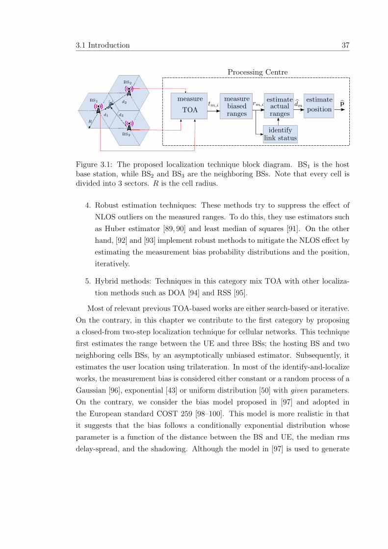
3.1 Introduction 37
d1
d2
d3
BS1
R
BS3
BS2
Processing Centre
measure
TOA
measurebiasedranges
estimateactualranges
identifylink status
estimate
positiontm,i rm,i dm p
Figure 3.1: The proposed localization technique block diagram. BS1 is the hostbase station, while BS2 and BS3 are the neighboring BSs. Note that every cell isdivided into 3 sectors. R is the cell radius.
4. Robust estimation techniques: These methods try to suppress the effect of
NLOS outliers on the measured ranges. To do this, they use estimators such
as Huber estimator [89, 90] and least median of squares [91]. On the other
hand, [92] and [93] implement robust methods to mitigate the NLOS effect by
estimating the measurement bias probability distributions and the position,
iteratively.
5. Hybrid methods: Techniques in this category mix TOA with other localiza-
tion methods such as DOA [94] and RSS [95].
Most of relevant previous TOA-based works are either search-based or iterative.
On the contrary, in this chapter we contribute to the first category by proposing
a closed-from two-step localization technique for cellular networks. This technique
first estimates the range between the UE and three BSs; the hosting BS and two
neighboring cells BSs, by an asymptotically unbiased estimator. Subsequently, it
estimates the user location using trilateration. In most of the identify-and-localize
works, the measurement bias is considered either constant or a random process of a
Gaussian [96], exponential [43] or uniform distribution [50] with given parameters.
On the contrary, we consider the bias model proposed in [97] and adopted in
the European standard COST 259 [98–100]. This model is more realistic in that
it suggests that the bias follows a conditionally exponential distribution whose
parameter is a function of the distance between the BS and UE, the median rms
delay-spread, and the shadowing. Although the model in [97] is used to generate

38 Mobile Localization under LOS/NLOS Conditions in Conventional Networks
simulation data in [55, 89], and [101], it was not incorporated in the respective
localization algorithm. In our work herein, we use this bias model knowledge
to derive an asymptotically unbiased estimator that finds approximate values of
the range between the UE and all the three BSs. To achieve this, a processing
center first collects TOA measurements and uses them to obtain range estimates
and identify the link status, as shown in Figure 3.1. Once all the three ranges
are estimated, they are used to define three circles. The closest three intersection
points of these circles are used to define a triangle whose centroid is taken as the
user location estimate. In case where two circles do not overlap, the center of
the gap between them is taken as a triangle vertex. To assess the performance of
our localization method, we investigate its performance in the four environments
classified in [97] as: Bad urban, urban, suburban, and rural.
The contributions and merits of this chapter can be summarized as
� In contrast to [55, 89], and [101], we use a range-dependent bias model [97]
to derive a TOA-based closed-form range estimator that is asymptotically
unbiased. Subsequently, we use trilateration to obtain an estimator of the
UE location in a closed-form.
� The MSE of the range estimator is derived and compared to the CRLB, which
we evaluate numerically1. The range PDF for the three BS is derived herein,
and is used to determine the average CRLB.
� Finally, extensive Monte-Carlo simulations are carried out to assess the per-
formance of the proposed localization technique in the four environments
mentioned above, using the performance measures defined in Section 3.5.
The results show that the proposed localization technique performs on aver-
age close to the CRLB.
The rest of the chapter is organized as follows: Section 3.2 presents the problem
formulation and sets the assumptions of this work. Subsequently, Section 3.3,
describes in detail the range estimator and shows its unbiased behavior, while
Section 3.4 explains the trilateration procedure of estimating the user location.
1We resort to numerical computation due to the difficulties in evaluating it analytically. Thesedifficulties are discussed in Section 3.5.

3.2 Problem Formulation 39
Host
Figure 3.2: BS selection is based on the sector of the host BS that the mobile isin. Three scenarios are possible as illustrated: White, light grey and dark grey.
Section 3.5 discusses the CRLB and the difficulties of obtaining it analytically. It
also lists the PDF of the range and defines the performance measure we use for
our technique assessment. The numerical results of the Monte-Carlo simulation are
given in Section 3.6. A thorough discussion of the results is also included in that
section. Finally, the conclusions are presented in Section 3.7.
3.2 Problem Formulation
In this section, we formulate the problem under consideration. Firstly, we present
the assumptions of our work, before discussing the signal model.
3.2.1 Assumptions
This work is based on the following assumptions:
� TOA measurements are readily available at the processing center, and were
obtained by the TOA method used by the air interface i.e., wireless standard.
The `th TOA measurement, τ`, is used to calculate the `th range, r` = τ`c,
where c = 3× 10⁸ m/s is the speed of the signal.
� As shown in Figure 3.2, we consider a cellular network with regular hexagonal

40 Mobile Localization under LOS/NLOS Conditions in Conventional Networks
cells. Each cell is divided into three sectors2. The user position is uniformly
distributed in the cell, and the sector in which the user exists is assumed to
be known. This can be identified using hand-over information available at the
processing center, as used in [89]. The sector boundaries are used to select
the three BSs to perform localization. In other words, considering the host
cell in Figure 3.2, when the UE is in a particular sector, the BSs in the cells
shaded with the corresponding color are selected to perform the localization.
As a result from the hexagonal pattern, BSs locations are also assumed to be
given. The backhaul link between BSs and processing center is assumed to
be error-free.
� Similar to [55] and [89], the measurement bias due to NLOS is modeled as an
exponential random process conditional to a zero-mean log-normal random
process. These distributions are described by the nature of the environment
as detailed in [97]. Consecutive bias samples are considered independent and
identically distributed (i.i.d). On the other hand, the measurement noise
is assumed to be i.i.d zero-mean Gaussian process, and independent of the
measurement bias.
� The parameters specifying the environment surrounding the UE are consid-
ered known and fixed during the measurements acquisition phase. The status
of each UE-BS link whether LOS or NLOS is assumed to stay unchanged dur-
ing the measurements acquisition phase.
3.2.2 Signal Model
Based on the above assumptions the ith range measurement at the mth BS can be
written as
rm,i = dm + nm,i + bm,i, i = 1, 2, ...Ns, m = 1, 2, 3. (3.1)
2A sector is a partial area of a cell that is served by a directional antenna, usually withbeamwidth of 60◦ or 120◦ [102].

3.2 Problem Formulation 41
where Ns is the sample size. The actual distance between the UE and the mth BS,
positioned at p = [px, py]T and pm = [px,m, py,m]T, respectively is given by
dm = ‖p− pm‖ =√
(px − px,m)2 + (py − py,m)2. (3.2)
Here, dm is an unknown variable that is considered constant over the Ns mea-
surements. nm,i denotes the measurement noise and is modeled as a zero-mean
Gaussian random variable, i.e., nm,i ∼ N (0, σ2n). The measurement bias, which is
always non-negative, is denoted by bm,i. In fact, bm,i = 0 in the case of a LOS
link between UE and the BS. On the other hand, bm,i is a positive random variable
under NLOS conditions. This is due to the fact that a signal reflected by obstacles
will travel a longer distance compared to a LOS signal. According to [97], the
stochastic distribution of bm,i is given by
fBm(bm,i) =
{0, LOS,∫∞
0+fBm|Zm(bm,i|zm)fZm(zm)dzm, NLOS,
(3.3)
where,
fZm(zm) =1
zmσz√
2πe− (ln zm)2
2σ2z , (3.4)
is the PDF of Zm, the lognormal random variable representing the shadowing that
affects the signal from the UE to the mth BS, σz is measured in nepers (σ′z[dB] =
σz20
ln 10), and
fBm|Z,(bm,i|zm) =1
κme−
bm,iκm . (3.5)
The parameter κm is given by
κm = cτrms = cT√dmzm, (3.6)
where τrms is the rms delay-spread within the UE environment, and T is the median
value of τrms obtained at a distance of 1 km from the BS.
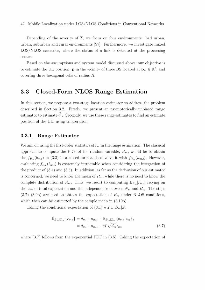
42 Mobile Localization under LOS/NLOS Conditions in Conventional Networks
Depending of the severity of T , we focus on four environments: bad urban,
urban, suburban and rural environments [97]. Furthermore, we investigate mixed
LOS/NLOS scenarios, where the status of a link is detected at the processing
center.
Based on the assumptions and system model discussed above, our objective is
to estimate the UE position, p in the vicinity of three BS located at pm ∈ R2, and
covering three hexagonal cells of radius R.
3.3 Closed-Form NLOS Range Estimation
In this section, we propose a two-stage location estimator to address the problem
described in Section 3.2. Firstly, we present an asymptotically unbiased range
estimator to estimate dm. Secondly, we use these range estimates to find an estimate
position of the UE, using trilateration.
3.3.1 Range Estimator
We aim on using the first-order statistics of rm in the range estimation. The classical
approach to compute the PDF of the random variable, Rm, would be to obtain
the fBm(bm,i) in (3.3) in a closed-form and convolve it with fNm(nm,i). However,
evaluating fBm(bm,i) is extremely intractable when considering the integration of
the product of (3.4) and (3.5). In addition, as far as the derivation of our estimator
is concerned, we need to know the mean of Rm, while there is no need to know the
complete distribution of Rm. Thus, we resort to computing ERm [rm,i] relying on
the law of total expectation and the independence between Nm and Bm. The steps
(3.7)–(3.9b) are used to obtain the expectation of Rm under NLOS conditions,
which then can be estimated by the sample mean in (3.10b).
Taking the conditional expectation of (3.1) w.r.t. Bm|Zm
EBm|Zm {rm,i} = dm + nm,i + EBm|Zm {bm,i|zm} ,= dm + nm,i + cT
√dmzm, (3.7)
where (3.7) follows from the exponential PDF in (3.5). Taking the expectation of

3.3 Closed-Form NLOS Range Estimation 43
(3.7) w.r.t Zm, and applying the law of total expectation [103]
EZm{EBm|Zm{rm,i}
}= EBm {rm,i} = dm + nm,i + cT
√dmµz, (3.8)
where µz = eσ2z2 is the mean of the log-normal distribution given in (3.4).
Taking the expectation of (3.8) with respect to Nm
ENm {EBm{rm,i}} = EBm,Nm{rm,i}, (3.9a)
= ERm{rm,i} = dm + cT√dmµz. (3.9b)
Note that (3.9a) follows from the assumption that the measurement noise and the
bias are independent, while (3.9b) uses the assumption that the noise is zero-mean.
It should be remarked that (3.9b) represents the theoretical mean of the collected
measurement, which requires infinite number of samples to be computed. Thus,
assuming ergodicity, we use the sample mean, given by
ERm{rm,i} , rm =1
Ns
Ns∑
i=1
rm,i, (3.10a)
= dm +1
Ns
Ns∑
i=1
bm,i. (3.10b)
instead, as a suitable estimate to the mean in (3.9b). This estimator is known to
be the best mean estimator as shown in [81].
Based on the sample mean of Rm, we now proceed to derive the closed-form
range estimator. Using (3.9b), and (3.10a), we can write
dm + cTµz
√dm − rm = 0. (3.11)
Equation (3.11) can be seen as a quadratic equation of
√dm ≥ 0, which can be
solved to obtain
√dm =
−cTµz +√
(cTµz)2 + 4rm2
. (3.12)

44 Mobile Localization under LOS/NLOS Conditions in Conventional Networks
Defining the parameter T , cTµz , we write
dm =
12
(T
2 − T√T
2+ 4rm
)+ rm, NLOS,
rm, LOS,(3.13)
Note that when T = 0, the NLOS estimator reduces to the LOS estimator. More-
over, note that since dm and bm,i are positive, rm is positive. As a result,
√T
2+ 4rm
is always real.
Proposition 3.1 The proposed range estimator under NLOS in (3.13) is asymp-
totically unbiased.
Proof
Using the assumption of zero-mean noise, and substituting (3.10b) in (3.13)
dm − dm =1
2
(T
2 − T
√√√√T2
+ 4dm +4
Ns
Ns∑
i=1
bm,i
)+
1
Ns
Ns∑
i=1
bm,i. (3.14)
Taking the expectation3 of (3.14)
E{dm} − dm =1
2E
T
2 − T
√√√√T2
+ 4dm +4
Ns
Ns∑
i=1
bm,i
+
1
Ns
Ns∑
i=1
E{bm,i}. (3.15)
If Ns is large enough, then
1
Ns
Ns∑
i=1
bm,i → E{bm,i} = Ez{κm} = T√dm, (3.16)
which implies that
E{dm} − dm →1
2
(T
2 − T√T
2+ 4dm + 4D
√dm
)+ T
√dm. (3.17)
3Dropping the subscript from the expectation operator means that the expectation is takenwith respect to the random variable between brackets.
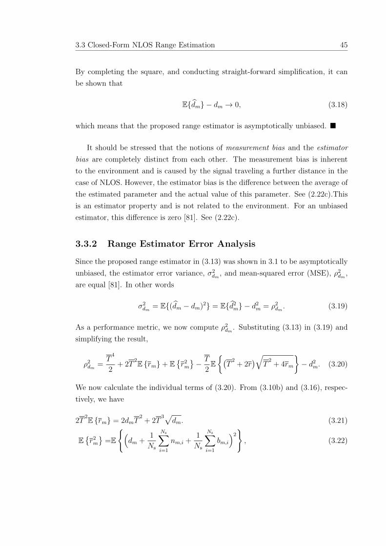
3.3 Closed-Form NLOS Range Estimation 45
By completing the square, and conducting straight-forward simplification, it can
be shown that
E{dm} − dm → 0, (3.18)
which means that the proposed range estimator is asymptotically unbiased. �
It should be stressed that the notions of measurement bias and the estimator
bias are completely distinct from each other. The measurement bias is inherent
to the environment and is caused by the signal traveling a further distance in the
case of NLOS. However, the estimator bias is the difference between the average of
the estimated parameter and the actual value of this parameter. See (2.22c).This
is an estimator property and is not related to the environment. For an unbiased
estimator, this difference is zero [81]. See (2.22c).
3.3.2 Range Estimator Error Analysis
Since the proposed range estimator in (3.13) was shown in 3.1 to be asymptotically
unbiased, the estimator error variance, σ2dm
, and mean-squared error (MSE), ρ2dm
,
are equal [81]. In other words
σ2dm = E{(dm − dm)2} = E{d2
m} − d2m = ρ2
dm . (3.19)
As a performance metric, we now compute ρ2dm
. Substituting (3.13) in (3.19) and
simplifying the result,
ρ2dm =
T4
2+ 2T
2E {rm}+ E{r2m
}− T
2E{(T
2+ 2r
)√T
2+ 4rm
}− d2
m. (3.20)
We now calculate the individual terms of (3.20). From (3.10b) and (3.16), respec-
tively, we have
2T2E {rm} = 2dmT
2+ 2T
3√dm. (3.21)
E{r2m
}=E
{(dm +
1
Ns
Ns∑
i=1
nm,i +1
Ns
Ns∑
i=1
bm,i
)2}, (3.22)

46 Mobile Localization under LOS/NLOS Conditions in Conventional Networks
=d2m +
1
N2s
E
{( Ns∑
i=1
nm,i
)2}
+1
N2s
E
{( Ns∑
i=1
bm,i
)2}
+2dmNs
Ns∑
i=1
E {bm,i} , (3.23)
=d2m +
1
N2s
E
{Ns∑
i=1
n2m,i
}+
1
N2s
E
{Ns∑
i=1
b2m,i + 2
Ns∑
i=1
Ns∑
j=i+1
bm,ibm,j
}+ 2dmT
√dm,
=d2m +
σ2n
Ns
+E{b2m,i
}
Ns
+(Ns − 1)E2 {bm,i}
Ns
+ 2dmT√dm,
=d2m + 2dmT
√dm +
σ2n + σ2
b
Ns
+ E2 {bm,i} ,
=d2m + T
2dm + 2dmT
√dm +
σ2n + σ2
b
Ns
. (3.24)
Note that the terms 2dmNs
∑Ns
i=1 E {nm,i} and 1N2
s
∑Ns
i=1 E {nm,i}∑Ns
i=1 E {bm,i} vanish
in (3.23) since the noise is zero-mean. Here, σ2b is the measurement bias variance
calculated by
σ2b = E
{b2m,i
}− E2 {bm,i} ,
= EZ{EB|Z
{b2m,i|zm
}}− E2
Z
{EB|Z {bm,i|zm}
},
= EZ{σ2B|Z + E2
B|Z {bm,i|zm}}− E2
z
{EB|Z {bm,i|zm}
},
= EZ{c2T 2dmz
2m + c2T 2dmz
2m
}− (cT
√dmµz)
2 = T2dm(2µ2
z − 1). (3.25)
Furthermore, using (3.10b) and (3.16), we can write
E{(T
2+ 2r
)√T
2+ 4rm
}=(T
2+ 2dm + 2T
√dm
)√T
2+ 4dm + 4T
√dm,
=(T
2+ 2dm + 2T
√dm
)(T + 2
√dm
),
= T3
+ 4T2√
dm + 6Tdm + 4dm√dm. (3.26)
Finally, substituting (3.21), (3.24) and (3.26) into (3.20) yields
ρ2dm =
1
Ns
T2(2µ2
z − 1)dm +1
Ns
σ2n, Ns � 1. (3.27)

3.4 Localization Based on Range Estimates 47
In summary, the asymptotic MSE is given by
ρ2dm =
T2(2µ2z−1)dm+σ2
n
Ns, NLOS,
σ2n
Ns, LOS,
(3.28)
Note that in the case of LOS, i.e., T = 0, ρ2dm
reduces to the well-known CRLB of
measurements contaminated by additive white Gaussian noise, σ2n/Ns [81].
3.4 Localization Based on Range Estimates
After estimating the range between every BS and the UE, we proceed to estimate
the UE location by, first, drawing circles with the estimated ranges, dm, as radii.
Then, we find the number of intersecting circles, denoted by C ≥ 0, and the points
of intersection of these circles. Two circles i, j are overlapping if
di + dj > ‖pi − pj‖. (3.29)
Subsequently, we define a triangle and estimate the UE location as its centroid.
However, since our distance estimator is asymptotically unbiased. i.e., E[dm]→ dm,
for some measurements, the distance will be under-estimated dm < dm, while for
the other measurements, it will be over-estimated, dm > dm. However, on the
long run the average estimated distance, E[dm], approaches the actual distance,
dm. These two cases are depicted in Figure 3.3, depending on which the triangle is
defined:
1. Case 1: Three intersecting circles (C = 3)
In this case, the triangle vertices are defined by the three intersection points
bounding the intersection area, as shown in Figure 3.3.(a). The three triangle
vertices are given by
v1 = arg minu∈{c(1)12 ,c
(2)12 }‖u− p3‖, (3.30)
v2 = arg minu∈{c(1)23 ,c
(2)23 }‖u− p1‖, (3.31)

48 Mobile Localization under LOS/NLOS Conditions in Conventional Networks
*
*
(a) (b)
d1
d2
d3p3
p2
p1 p3
p2
p1
d1
d2
d3
d1
d2
d3d1
d2
d3
p p Triangle vertices
v3
v2
v1
v3
v2v1
Figure 3.3: Effect of range estimation error on location estimation (a) C = 3 and(b) C = 2.
v3 = arg minu∈{c(1)31 ,c
(2)31 }‖u− p2‖, (3.32)
where c(1)ij , c
(2)ij ∈ R2 are the two intersection points of the circles i and j.
2. Case 2: Less than three intersecting circles (C < 3)
Because less than three circles overlap, three intersection points are partially
available. To decide on triangle vertices, the circles are investigated in pairs.
Since any two intersecting circles will have two intersection points, we define
a triangle vertex by the intersection point closer to the third circle (non-
intersecting), similar to (3.30) – (3.32). For the non-overlapping circles, we
define the triangle vertex as the point in the gap center between the two
circles. For the example illustrated in Figure 3.3.(b), two circles overlap, but
a third point is needed for trilateration. Thus, we select the mid-gap point
as a reasonable heuristic approach.
v3 = p1 + (d1 + 0.5g)p3 − p1
‖p3 − p1‖, (3.33)
where g = (d1 + d3)− ‖p3 − p1‖, is the gap between the two circles. To see
why this approach is taken, consider Figure 3.3.(b). Circle 1 and circle 3 do

3.5 Cramer-Rao Lower Bound 49
not overlap. This means that d1, d3, or both are under-estimated. However,
we have no additional information to weigh among the three possibilities. For
this reason, we choose the mid-gap point as a trilateration point.
After obtaining the triangle vertices, v1,v2 and v3, the UE location is estimated
by
p =1
3(v1 + v2 + v3). (3.34)
3.5 Cramer-Rao Lower Bound
Discussed in Chapter 2, CRLB is one of the most important performance bench-
mark for an estimator. In our problem, the CRLB of dm in (3.1) is defined by [81]
CRLB(dm) =−1
E[∂2 ln f(rm;dm)
∂2dm
] , (3.35)
where rm = [rm,1, rm,2, ..., rm,Ns ]T . Note that in the classical case of LOS, this
bound is given by σ2n/Ns [81]. Although there has been some works on CRLB for
NLOS localization, e.g., [54] and [93], none of these works addressed the problem
formulated in Section 3.2. Therefore, in this section, we focus on NLOS CRLB.
To start with, we need the joint probability distribution f(rm; dm). However,
since rm,1, rm,2, ..., rm,Ns are i.i.d, we can write
f(rm; dm) =Ns∏
i=1
f(rm,i; dm) = fNs(rm,1; dm), (3.36)
where the first equality follows from the independence assumption, and the sec-
ond equality follows from the identical distribution assumption. Without loss of
generality, we choose PDF pf the first sample, rm,1. We make the following remarks,
� rm,1 = (dm + nm,1) + bm,1, so to evaluate f(rm,1; dm), we would require the
joint probability fB,N+D(b, n+ dm).
� From (3.1), bm,1 and dm + nm,1 are not independent since bm,1 is a function

50 Mobile Localization under LOS/NLOS Conditions in Conventional Networks
Algorithm 1 Numerical Evaluation of CRLB in (3.35), using MATLAB
Input Ns, σn, σz, R, T, c,Nb, Ir, Icrlb.initialize CRLB(dm) = 0,∀dmfor k = 1 : Icrlb do
for dm = 1 : 2R doinitialize f(r; dm) = 0Generate zmfor i = 1 : Ir do
Generate Nb instances of bm,i, and nm,i,Calculate the corresponding Nb instances of rm,i = dm + bm,i + nm,i,
Obtain the Kernel Density Estimate,f(ri; dm), using a a normal kernel function [104].
f(r; dm) = f(r; dm) + f(ri; dm)end forf(r; dm) = f(r; dm)/Ir
end forfor j = 1 : Nb do
g(j, dm) = ∂2
∂d2m
ln f(j; dm), where the second derivative is obtained by the MATLAB
function diff(.,2)
end forCRLB(dm) = CRLB(dm) + −1
Ns∑
j g(j,dm)f(j;dm)
end forCRLB(dm) = CRLB(dm)/Icrlb.
of dm. Therefore, their joint distribution cannot be simply obtained by the
convolution of the marginal distribution, fB(b) and dm-shifted fN(n).
� Even if they were independent, the integral in (3.3) is very hard to evaluate
from (3.4) and (3.5).
For these reasons, we proceed to evaluate the CRLB numerically as listed in Algo-
rithm 1.
The CRLB procedure in Algorithm 1 gives a performance measure for individ-
ual range estimators. However, to evaluate the overall localization performance,
we need to define some performance measures that take into account the average
performance over the three cells. But before that, we need to evaluate the PDF of
the range, fD(dm), for m = 1, 2, 3. As derived in Appendix A, for the hosting cell

3.5 Cramer-Rao Lower Bound 51
0 100 200 300 400 500 600 700 800 900 1,0000
1
2
3
4
·10−3
d (m)
f D(d
m)
m = 1m = 2, 3
Figure 3.4: PDF of the UE range from the mth BS, m = 1, 2 and 3. R = 500 m.
(m = 1), this distribution is given by
fD(dm) =
4πdm3√
3R2 , 0 ≤ dm <√
3R2,
8dm√3R2
[π6− cos−1
(√
3R2dm
)],√
32R ≤ dm < R.
(3.37)
For the two neighboring cells (m = 2, 3), this distribution is given by
fD(dm) =
4dm√3R2 cos−1
(√3R
2dm
),
√3R2≤ dm < R
2dm√3R2 sin−1
(√3R
2dm
), R ≤ dm <
√3R
2dm√3R2
[sin−1
(√3Rdm
)− π
3
],√
3R ≤ dm < 2R
(3.38)
Figure 3.4 shows the plots of (3.37) and (3.38) for a cell with radius of 500 m.
To measure the performance averaged over the three cells, we define the follow-
ing measures:
� Average CRLB over three cells:
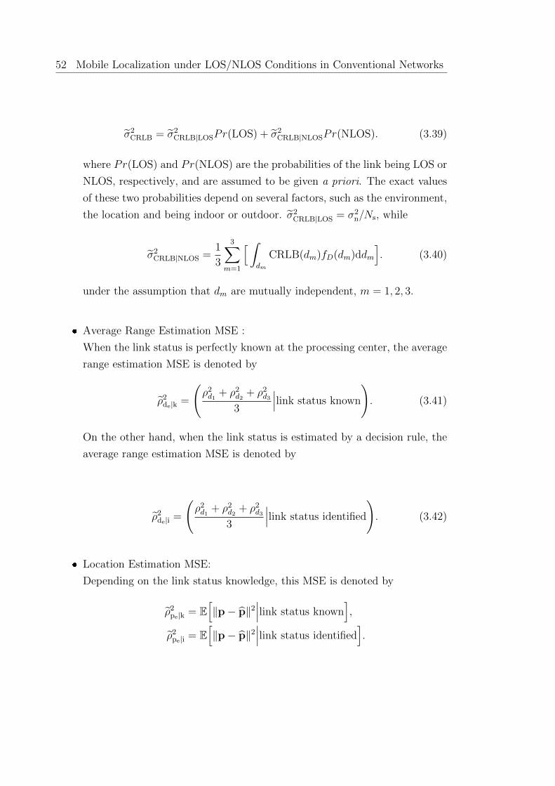
52 Mobile Localization under LOS/NLOS Conditions in Conventional Networks
σ2CRLB = σ2
CRLB|LOSPr(LOS) + σ2CRLB|NLOSPr(NLOS). (3.39)
where Pr(LOS) and Pr(NLOS) are the probabilities of the link being LOS or
NLOS, respectively, and are assumed to be given a priori. The exact values
of these two probabilities depend on several factors, such as the environment,
the location and being indoor or outdoor. σ2CRLB|LOS = σ2
n/Ns, while
σ2CRLB|NLOS =
1
3
3∑
m=1
[ ∫
dm
CRLB(dm)fD(dm)ddm
]. (3.40)
under the assumption that dm are mutually independent, m = 1, 2, 3.
� Average Range Estimation MSE :
When the link status is perfectly known at the processing center, the average
range estimation MSE is denoted by
ρ2de|k =
(ρ2d1
+ ρ2d2
+ ρ2d3
3
∣∣∣link status known
). (3.41)
On the other hand, when the link status is estimated by a decision rule, the
average range estimation MSE is denoted by
ρ2de|i =
(ρ2d1
+ ρ2d2
+ ρ2d3
3
∣∣∣link status identified
). (3.42)
� Location Estimation MSE:
Depending on the link status knowledge, this MSE is denoted by
ρ2pe|k = E
[‖p− p‖2
∣∣∣link status known],
ρ2pe|i = E
[‖p− p‖2
∣∣∣link status identified].
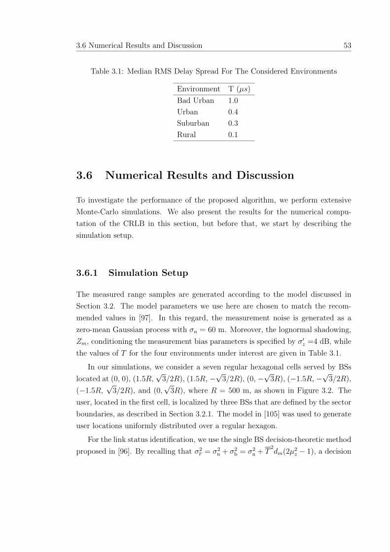
3.6 Numerical Results and Discussion 53
Table 3.1: Median RMS Delay Spread For The Considered Environments
Environment T (µs)
Bad Urban 1.0
Urban 0.4
Suburban 0.3
Rural 0.1
3.6 Numerical Results and Discussion
To investigate the performance of the proposed algorithm, we perform extensive
Monte-Carlo simulations. We also present the results for the numerical compu-
tation of the CRLB in this section, but before that, we start by describing the
simulation setup.
3.6.1 Simulation Setup
The measured range samples are generated according to the model discussed in
Section 3.2. The model parameters we use here are chosen to match the recom-
mended values in [97]. In this regard, the measurement noise is generated as a
zero-mean Gaussian process with σn = 60 m. Moreover, the lognormal shadowing,
Zm, conditioning the measurement bias parameters is specified by σ′z =4 dB, while
the values of T for the four environments under interest are given in Table 3.1.
In our simulations, we consider a seven regular hexagonal cells served by BSs
located at (0, 0), (1.5R,√
3/2R), (1.5R, −√
3/2R), (0, −√
3R), (−1.5R, −√
3/2R),
(−1.5R,√
3/2R), and (0,√
3R), where R = 500 m, as shown in Figure 3.2. The
user, located in the first cell, is localized by three BSs that are defined by the sector
boundaries, as described in Section 3.2.1. The model in [105] was used to generate
user locations uniformly distributed over a regular hexagon.
For the link status identification, we use the single BS decision-theoretic method
proposed in [96]. By recalling that σ2r = σ2
n + σ2b = σ2
n + T2dm(2µ2
z − 1), a decision
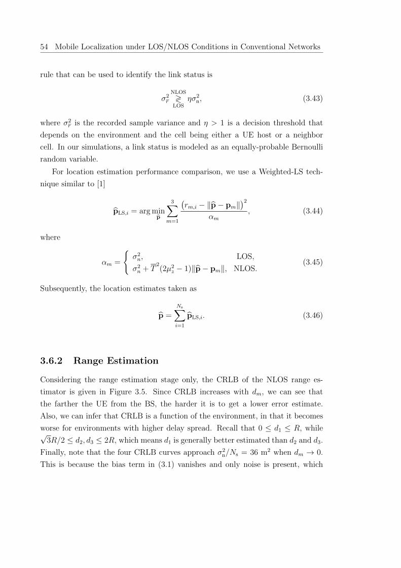
54 Mobile Localization under LOS/NLOS Conditions in Conventional Networks
rule that can be used to identify the link status is
σ2r
NLOS
≷LOS
ησ2n, (3.43)
where σ2r is the recorded sample variance and η > 1 is a decision threshold that
depends on the environment and the cell being either a UE host or a neighbor
cell. In our simulations, a link status is modeled as an equally-probable Bernoulli
random variable.
For location estimation performance comparison, we use a Weighted-LS tech-
nique similar to [1]
pLS,i = arg minp
3∑
m=1
(rm,i − ‖p− pm‖
)2
αm, (3.44)
where
αm =
{σ2n, LOS,
σ2n + T
2(2µ2
z − 1)‖p− pm‖, NLOS.(3.45)
Subsequently, the location estimates taken as
p =Ns∑
i=1
pLS,i. (3.46)
3.6.2 Range Estimation
Considering the range estimation stage only, the CRLB of the NLOS range es-
timator is given in Figure 3.5. Since CRLB increases with dm, we can see that
the farther the UE from the BS, the harder it is to get a lower error estimate.
Also, we can infer that CRLB is a function of the environment, in that it becomes
worse for environments with higher delay spread. Recall that 0 ≤ d1 ≤ R, while√3R/2 ≤ d2, d3 ≤ 2R, which means d1 is generally better estimated than d2 and d3.
Finally, note that the four CRLB curves approach σ2n/Ns = 36 m2 when dm → 0.
This is because the bias term in (3.1) vanishes and only noise is present, which
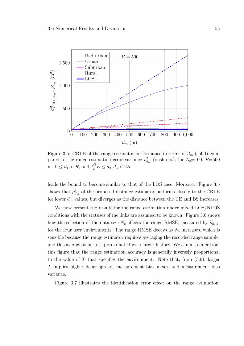
3.6 Numerical Results and Discussion 55
0 100 200 300 400 500 600 700 800 900 1,0000
500
1,000
1,500
dm (m)
σ2 CRLB,d
m,ρ2 dm(m
2)
Bad urbanUrbanSuburbanRuralLOS
R = 500
Figure 3.5: CRLB of the range estimator performance in terms of dm (solid) com-pared to the range estimation error variance ρ2
dm(dash-dot), for Ns=100, R=500
m. 0 ≤ d1 < R, and√
32R ≤ d2, d3 < 2R
leads the bound to become similar to that of the LOS case. Moreover, Figure 3.5
shows that ρ2dm
of the proposed distance estimator performs closely to the CRLB
for lower dm values, but diverges as the distance between the UE and BS increases.
We now present the results for the range estimation under mixed LOS/NLOS
conditions with the statuses of the links are assumed to be known. Figure 3.6 shows
how the selection of the data size Ns affects the range RMSE, measured by ρde|k,
for the four user environments. The range RMSE decays as Ns increases, which is
sensible because the range estimator requires averaging the recorded range sample,
and this average is better approximated with larger history. We can also infer from
this figure that the range estimation accuracy is generally inversely proportional
to the value of T that specifies the environment. Note that, from (3.6), larger
T implies higher delay spread, measurement bias mean, and measurement bias
variance.
Figure 3.7 illustrates the identification error effect on the range estimation.
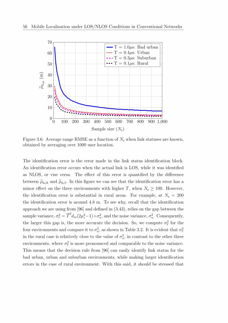
56 Mobile Localization under LOS/NLOS Conditions in Conventional Networks
0 100 200 300 400 500 600 700 800 900 1,0000
10
20
30
40
50
60
70
Sample size (Ns)
ρde|k(m
)
T = 1.0µs: Bad urbanT = 0.4µs: UrbanT = 0.3µs: SuburbanT = 0.1µs: Rural
Figure 3.6: Average range RMSE as a function of Ns when link statuses are known,obtained by averaging over 1000 user location.
The identification error is the error made in the link status identification block.
An identification error occurs when the actual link is LOS, while it was identified
as NLOS, or vise versa. The effect of this error is quantified by the difference
between ρde|k and ρde|i. In this figure we can see that the identification error has a
minor effect on the three environments with higher T , when Ns ≥ 100. However,
the identification error is substantial in rural areas. For example, at Ns = 200
the identification error is around 4.8 m. To see why, recall that the identification
approach we are using from [96] and defined in (3.43), relies on the gap between the
sample variance, σ2r = T
2dm(2µ2
z−1)+σ2n, and the noise variance, σ2
n. Consequently,
the larger this gap is, the more accurate the decision. So, we compute σ2r for the
four environments and compare it to σ2n, as shown in Table 3.2. It is evident that σ2
r
in the rural case is relatively close to the value of σ2n, in contrast to the other three
environments, where σ2r is more pronounced and comparable to the noise variance.
This means that the decision rule from [96] can easily identify link status for the
bad urban, urban and suburban environments, while making larger identification
errors in the case of rural environment. With this said, it should be stressed that
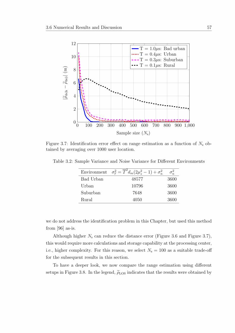
3.6 Numerical Results and Discussion 57
0 100 200 300 400 500 600 700 800 900 1,0000
2
4
6
8
10
12
Sample size (Ns)
|ρde|k−ρde|i|(m)
T = 1.0µs: Bad urbanT = 0.4µs: UrbanT = 0.3µs: SuburbanT = 0.1µs: Rural
Figure 3.7: Identification error effect on range estimation as a function of Ns ob-tained by averaging over 1000 user location.
Table 3.2: Sample Variance and Noise Variance for Different Environments
Environment σ2r = T
2dm(2µ2
z − 1) + σ2n σ2
n
Bad Urban 48577 3600
Urban 10796 3600
Suburban 7648 3600
Rural 4050 3600
we do not address the identification problem in this Chapter, but used this method
from [96] as-is.
Although higher Ns can reduce the distance error (Figure 3.6 and Figure 3.7),
this would require more calculations and storage capability at the processing center,
i.e., higher complexity. For this reason, we select Ns = 100 as a suitable trade-off
for the subsequent results in this section.
To have a deeper look, we now compare the range estimation using different
setups in Figure 3.8. In the legend, ρLOS indicates that the results were obtained by

58 Mobile Localization under LOS/NLOS Conditions in Conventional Networks
100
101
102
103
Bad Urban Urban Suburban Rural
ρde(m
)ρLOS
ρNLOS
ρde|iρde|kσCRLB
Figure 3.8: Average RMSE of range error in different setups compared to averageCRLB, obtained by averaging over 1000 user location with Ns = 100.
the averaging estimator that assumes that all the links are LOS [81], i.e., ignoring
the existence of NLOS paths. On the contrary, ρNLOS is obtained by the estimator in
(3.13) that assumes that all the paths are NLOS, i.e., assumes measurement bias
exists in all paths. ρde|i, ρde|k, and σCRLB are the square roots of the quantities
defined in (3.42), (3.41), and (3.39), respectively.
It can be concluded from Figure 3.8 that, when link identification is imple-
mented, the proposed estimator performs close to σCRLB with difference of 3.1 m,
1.9 m, 3.2 m, and 6.5 m in the bad urban, urban, suburban, and rural environ-
ments, respectively. Smaller gaps occur when the link status is perfectly known at
the processing center, with the performance of the proposed technique approach
the CRLB for the suburban and rural areas. Also, notice that the error upper-
bound is well above the proposed estimator error. On an absolute measure, the
proposed estimator provides range estimates with ρde|i of: 21.4 m, 10.9 m, 10.1 m,
and 13.0 m in the four environments, respectively.
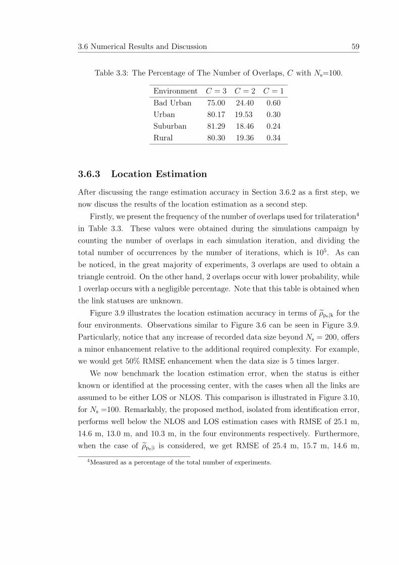
3.6 Numerical Results and Discussion 59
Table 3.3: The Percentage of The Number of Overlaps, C with Ns=100.
Environment C = 3 C = 2 C = 1
Bad Urban 75.00 24.40 0.60
Urban 80.17 19.53 0.30
Suburban 81.29 18.46 0.24
Rural 80.30 19.36 0.34
3.6.3 Location Estimation
After discussing the range estimation accuracy in Section 3.6.2 as a first step, we
now discuss the results of the location estimation as a second step.
Firstly, we present the frequency of the number of overlaps used for trilateration4
in Table 3.3. These values were obtained during the simulations campaign by
counting the number of overlaps in each simulation iteration, and dividing the
total number of occurrences by the number of iterations, which is 105. As can
be noticed, in the great majority of experiments, 3 overlaps are used to obtain a
triangle centroid. On the other hand, 2 overlaps occur with lower probability, while
1 overlap occurs with a negligible percentage. Note that this table is obtained when
the link statuses are unknown.
Figure 3.9 illustrates the location estimation accuracy in terms of ρpe|k for the
four environments. Observations similar to Figure 3.6 can be seen in Figure 3.9.
Particularly, notice that any increase of recorded data size beyond Ns = 200, offers
a minor enhancement relative to the additional required complexity. For example,
we would get 50% RMSE enhancement when the data size is 5 times larger.
We now benchmark the location estimation error, when the status is either
known or identified at the processing center, with the cases when all the links are
assumed to be either LOS or NLOS. This comparison is illustrated in Figure 3.10,
for Ns =100. Remarkably, the proposed method, isolated from identification error,
performs well below the NLOS and LOS estimation cases with RMSE of 25.1 m,
14.6 m, 13.0 m, and 10.3 m, in the four environments respectively. Furthermore,
when the case of ρpe|i is considered, we get RMSE of 25.4 m, 15.7 m, 14.6 m,
4Measured as a percentage of the total number of experiments.
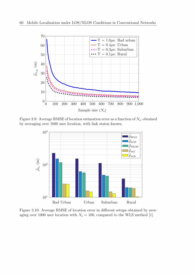
60 Mobile Localization under LOS/NLOS Conditions in Conventional Networks
0 100 200 300 400 500 600 700 800 900 1,0000
10
20
30
40
50
60
70
Sample size (Ns)
ρxe|k(m
)
T = 1.0µs: Bad urbanT = 0.4µs: UrbanT = 0.3µs: SuburbanT = 0.1µs: Rural
Figure 3.9: Average RMSE of location estimation error as a function ofNs, obtainedby averaging over 1000 user location, with link status known.
101
102
103
Bad Urban Urban Suburban Rural
ρxe(m
)
ρWLS
ρLOS
ρNLOS
ρxe|iρxe|k
Figure 3.10: Average RMSE of location error in different setups obtained by aver-aging over 1000 user location with Ns = 100, compared to the WLS method [1].

3.6 Numerical Results and Discussion 61
0 10 20 30 40 50 60 70 800
1
2
3
4
5
6
7·10−2
‖p− p‖
Pe
Bad urbanUrbanSuburbanRural
Figure 3.11: PDF of the location error with Ns =100, obtained by averaging over1000 user locations, with link status identified.
and 18.7 m, respectively. Since the error of a stage propagates to the subsequent
stage, it should be highlighted that the ρpe|i effect in Figure 3.10 comprises three
error components, namely: identification error, range estimation error and location
estimation error.
Finally, note that the proposed approach outperforms the WLS approach, de-
noted by ρWLS and outlined in (3.44)-(3.45), by a large margin. This is because our
approach takes into account the bias distribution function, in contrast to the one
in [1]. Also note that due to the bias being non-Gaussian, the numerator of (3.44)
is non-Gaussian. Moreover, WLS requires a higher number of BS for an accurate
estimate. These two reasons cause WLS to have a greater estimation error than
the other considered approaches in Figure 3.10.
To get a better insight on the nature of location error, Figure 3.11 illustrates
the approximate error distributions for the four environments obtained during the
simulations with identification. Again, note that this this error is the total error
due to identification error, ranging error, and localization error. It can be seen
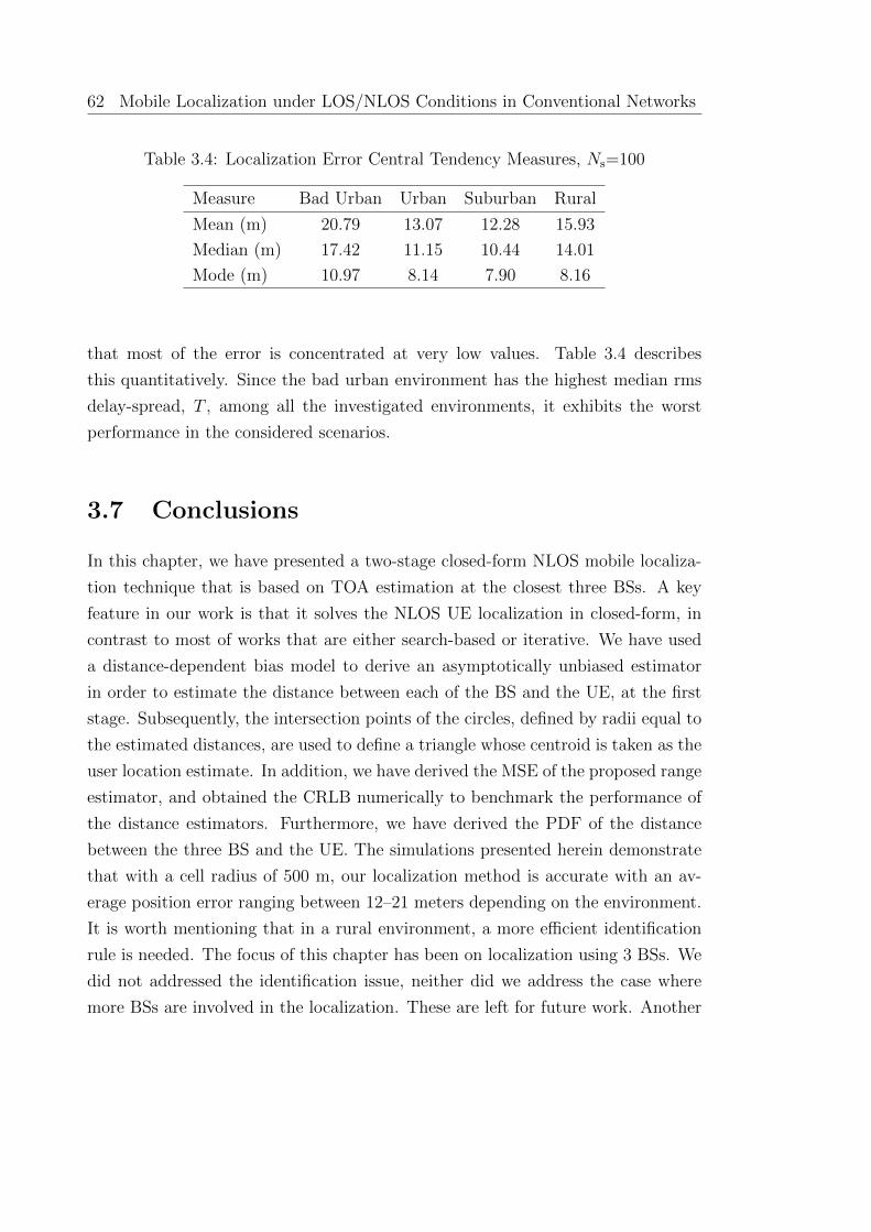
62 Mobile Localization under LOS/NLOS Conditions in Conventional Networks
Table 3.4: Localization Error Central Tendency Measures, Ns=100
Measure Bad Urban Urban Suburban Rural
Mean (m) 20.79 13.07 12.28 15.93
Median (m) 17.42 11.15 10.44 14.01
Mode (m) 10.97 8.14 7.90 8.16
that most of the error is concentrated at very low values. Table 3.4 describes
this quantitatively. Since the bad urban environment has the highest median rms
delay-spread, T , among all the investigated environments, it exhibits the worst
performance in the considered scenarios.
3.7 Conclusions
In this chapter, we have presented a two-stage closed-form NLOS mobile localiza-
tion technique that is based on TOA estimation at the closest three BSs. A key
feature in our work is that it solves the NLOS UE localization in closed-form, in
contrast to most of works that are either search-based or iterative. We have used
a distance-dependent bias model to derive an asymptotically unbiased estimator
in order to estimate the distance between each of the BS and the UE, at the first
stage. Subsequently, the intersection points of the circles, defined by radii equal to
the estimated distances, are used to define a triangle whose centroid is taken as the
user location estimate. In addition, we have derived the MSE of the proposed range
estimator, and obtained the CRLB numerically to benchmark the performance of
the distance estimators. Furthermore, we have derived the PDF of the distance
between the three BS and the UE. The simulations presented herein demonstrate
that with a cell radius of 500 m, our localization method is accurate with an av-
erage position error ranging between 12–21 meters depending on the environment.
It is worth mentioning that in a rural environment, a more efficient identification
rule is needed. The focus of this chapter has been on localization using 3 BSs. We
did not addressed the identification issue, neither did we address the case where
more BSs are involved in the localization. These are left for future work. Another

3.7 Conclusions 63
potential venue for investigation in the context of this Chapter is the application
of linearised solution of the TOA equations to obtain an estimate of the user lo-
cation, instead of taking the centroid of the intersection area. Moreover, since the
performance of the proposed technique in this Chapter is model-dependent, it is
meaningful to consider model mismatch analysis and simulation for future work.
Finally, we note that, even though the proposed technique performs closely with
the CRLB, the average error obtained is in the order of several meters, which im-
plies that location-aware communications have limited applications in conventional
cellular networks.
Publications Resulted from This Chapter
� Z. Abu-Shaban, X. Zhou, T. Abhayapala, “A Novel TOA-based Mobile Lo-
calization Technique under Mixed LOS/NLOS Conditions for Cellular Net-
works,” IEEE Transactions on Vehicular Technology, vol. 65, no. 11, pp.
8841-8853, Nov 2016.


Chapter 4
Beamforming for Initial Access in
5G mmWave Networks
Overview: The utilization of the millimeter-wave frequency band in 5G is a highly-
debated current topic. MmWave MIMO systems will use arrays with large number
of antennas at the transmitter and the receiver, implemented on a relatively small
area. With the inherent high directivity of these arrays, the initial access to the
network (IA) will be challenge in 5G mmWave, since using omni-directional trans-
mission is not feasible due to the high propagation loss. Therefore, algorithms to
help the UE find the BS and establish a communication link should be carefully
designed. Towards that, we examine two beamforming schemes, namely, random-
phase beamforming (RPBF) and directional beamforming (DBF), under the line-
of-sight channel model. Since the step following IA would be channel estimation,
we compare RPBF and DBF with respect to the the CRLB of jointly estimating the
channel parameters: DOA, DOD, TOA, and the complex channel gain. The results
show that the application of RPBF is more appropriate in the considered scenario
because it attains a lower CRLB with fewer beams compared to DBF.
4.1 Introduction
One of the enabling technologies of the fifth generation of mobile networks (5G)
is the millimeter-wave technology (mmWave) that operates at a carrier frequency
65

66 Beamforming for Initial Access in 5G mmWave Networks
in the range of 30–300 GHz [62–65,106]. MmWave allows packing high number of
antennas in a relatively small area due to their small wavelengths – from 1 mm
to 1 cm. In addition, the massively available spectrum of mmWave would easily
enable transmission with extremely high data rates [62]. Although 5G localization
research is still in its infancy, these two reasons reinforce the role that the mmWave
technology can play in 5G localization.
Due to the special characteristics of the mmWave channel, directional trans-
mission with large-size arrays, at both the transmitter and the receiver, is going to
be utilized [64]. However, when initiating a communication link, this high direc-
tionality is an issue for a user equipment (UE) trying to find the base station (BS),
or vice-versa, especially that omni-directional transmission with antenna arrays is
a challenge by itself [107,108].
The mmWave initial access (IA) techniques with analog beamforming were
reviewed in [72]. The three approaches compared therein include two direction-
based methods, namely exhaustive search and iterative search. The third method
is a GPS-assisted algorithm. The disadvantage of these approaches is mainly the
delay of finding the proper transmission direction through scanning the area of
interest.
Our approach in this thesis to consider the transmission of several beams si-
multaneously rather than scanning. The main advantage of such approach is that
it reduces the search time significantly with respect to the exhaustive search and
iterative search methods. This is particularly important in mmWave systems as
the 5G network will be designed for low-latency applications [61]. In contrast to
the directional beamforming, we focus on random beamforming. The concept of
random beamforming is not new per-se. Randomly-directional beamforming is a
method of opportunistic beamforming that was investigated for mmWave receivers
in [109,110]. Under this scheme, the BS generates narrow beams with random direc-
tions and select the user with the highest SNR. On the other hand, optimization-
based random beamforming in [108] optimizes the beamforming weights so that
the resulting beam pattern is omni-directional. The work therein focused on con-
ventional multiple-input-multiple-output (MIMO) systems in the microwave band.
Despite the advantage of omni-directional coverage in the AI phase, the cost func-
tion is complex and, for a high number of antennas, it is only solvable numerically.

4.2 Problem Formulation 67
Another random beamforming investigated under conventional MIMO is the uni-
tary beamforming, whereby the beamforming matrix is obtained by the singular
value decomposition of the channel matrix, e.g., see [111]. This is not applicable
in an IA scenario since the channel is unknown at that phase. Analog beamform-
ing in mmWave is implemented using phase-shifters only. Therefore, we limit our
beamforming to be unit-magnitude variable phase.
In this Chapter, we look into the IA problem for a LOS mmWave channel
and investigate a random beamforming scheme, referred to as random-phase beam-
forming (RPBF). Under this scheme, the beamforming vector is generated as a
vector of complex exponentials with i.i.d. random phases. This scheme is used
in [112] to initiate an iterative beamforming scheme which assumes full channel
knowledge, and in [113], which assumes the DOD to be known. However, these
two assumptions are not used in our work. We compare the RPBF with directional
beamforming (DBF) scheme. Since the step following a successful initial access
would be the channel estimation, it is meaningful to compare the performance of
these two schemes in terms of the CRLB of the channel parameters: DOA, DOD,
TOA, and the complex channel gain. The CRLB of a LOS mmWave channel pa-
rameters were previously studied in [114]. Therein, the CRLBs were provided as a
function of the Fisher information matrix (FIM), whose entries were given by high
level expressions and are valid for ULA . The current Chapter presents the closed-
form CRLB expressions of the mmWave parameter using ULA, simpler than those
obtained in [114]. Although mmWave may apply different array geometries, ULA
is the standard array structure that is usually used to get initial insights. Finally,
we investigate and assess the RPBF and DBF in terms of the CRLBs, as a function
of the number of transmit antennas, receive antennas and transmit beams.
While we focus on the IA herein, in subsequent Chapters, we focus on localiza-
tion performance and synchronization issues, beyond the initial access phase.
4.2 Problem Formulation
Consider the scenario illustrated in Figure 4.1, where the receiver and the transmit-
ter are equipped with arrays of NR and NT antennas, respectively. Without loss of
generality, we consider the uplink and assume that the BS and UE are located in the

68 Beamforming for Initial Access in 5G mmWave Networks
NT
φ0
UE
BS
NR
φR
φT
x
y
d1
Figure 4.1: A schematic diagram of the considered scenario. d1 is the transmitter-receiver separation distance.
same plane. Consequently, we consider a 2D approach. Moreover, similar to [114],
we assume that the UE and BS communicate via a LOS path only. We leave the
investigation of the NLOS where communication is carried out via scatterers and
reflectors to Chapter 5. Furthermore, we assume that the transmit antenna array
is rotated by an unknown orientation angle φ0. Finally, we assume that the arrays
are narrow-band, i.e., the signal traverses the antenna arrays apertures, both at
the transmitter and the receiver, within a fraction of a symbol duration. That is
Amax � cTs, where Amax is the maximum array aperture.
As described in Section 2.1.3, and based on the above assumptions, the channel
matrix is modeled by
H ,√NRNTβaR(φR)aH
T(φT) ∈ CNR×NT , (4.1)
where β = βR + jβI ∈ C is the complex channel gain, φR is the DOA, and φT is
the DOD. Under mmWave channel, DOD depends on the orientation angle and
both are crucial in beamforming, since the knowledge of the direction of departure
and the orientation angle would enable more efficient beamforming. From Section
2.1.1, for a receiver equipped with a ULA of NR elements placed along the x-axis

4.2 Problem Formulation 69
with d inter-element spacing, the array response vector is given by
aR(φR) =1√NR
e−j2πdλ
cosφRxR ∈ CNR , (4.2)
where xR is as defined in (2.9). Similarly, by using the subscript T, the transmitter
array steering vector is given by
aT(φT) =1√NT
e−j2πdλ
cosφTxT ∈ CNT . (4.3)
For notation simplicity, we drop the angle parameter from aR(φR) and aT(φT).
These two vectors are normalized so that ‖aR‖2 = ‖aT‖2 = 1. Thus, the received
signal at the analog output of the array at a time instant t, can be written as
r(t) , [r1(t), r2(t), ..., rNR(t)]T, ∈ CNR , t ∈ [0, To],
= Hx(t− τ) + n(t). (4.4)
where To ≈ NsTs is the observation time and Ns is the number of pilot sym-
bols. Moreover, τ ∈ R+ is the propagation delay of the transmitted signal,
i.e., TOA, and is related to the transmitter-receiver distance , by τ = d1/c.
Furthermore, n(t) , [n1(t), n2(t), ..., nNT(t)]T ∈ CNR denotes zero-mean additive
white Gaussian noise processes with spectral density (PSD) N0. Furthermore,
x(t) , [x1(t), x2(t), ..., xNT(t)]T ∈ CNT is the single-carrier transmitted signal vector
at the output of a beamforming matrix F , [f1, f2, ...fNB] such that x(t) =
√EtFs(t)
and s(t) , [s1(t), s2(t), ..., sNB(t)]T, where NB is the number of transmitted beams
and Et is the transmitted energy per symbol. Moreover,
s`(t) =Ns−1∑
k=0
a`,kp(t− kTs), ` = 1, ..., NB (4.5)
where a`,k is the kth pilot symbol transmitted over the `th beam, and p(t) is a unit-
energy pulse with a PSD |P (f)|2 and a bandwidth W . To keep the transmitted
power fixed, regardless of the number of antennas, NT, we normalize F such that
Tr(FHF
)= 1, and s(t)sH(t) = INB
. Matrix F is modeled in two ways: directional
and random. These models and the differences between them are discussed in detail
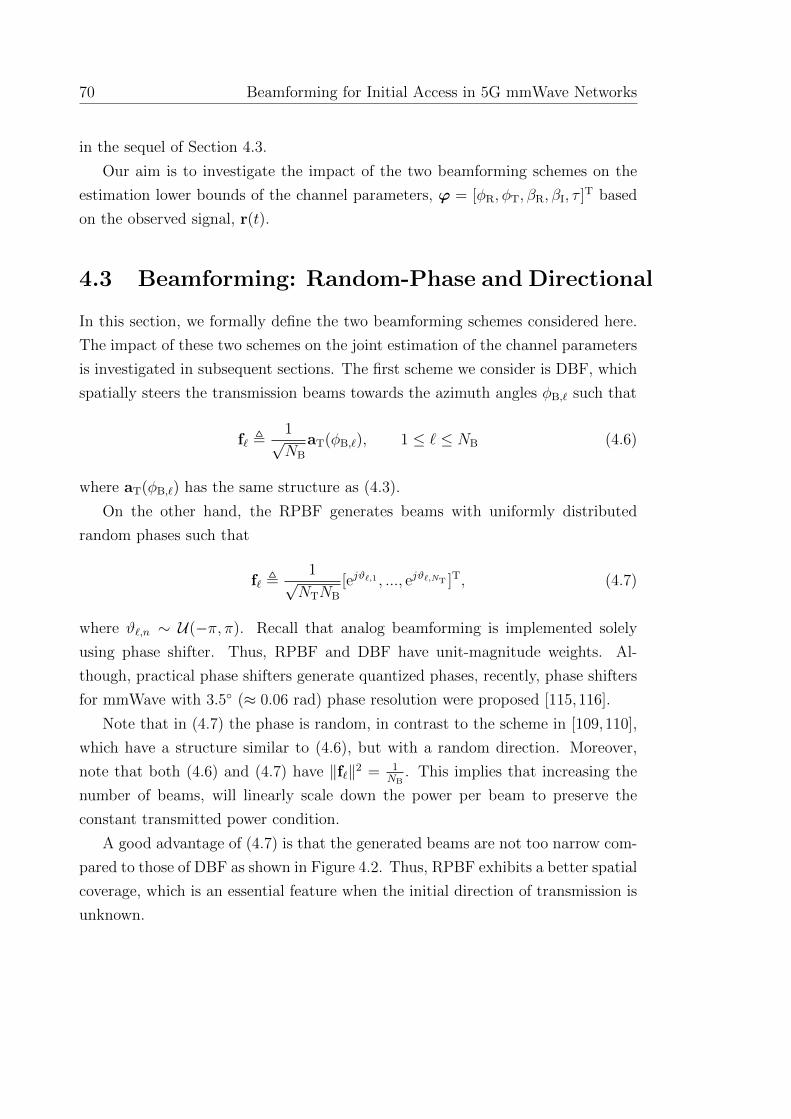
70 Beamforming for Initial Access in 5G mmWave Networks
in the sequel of Section 4.3.
Our aim is to investigate the impact of the two beamforming schemes on the
estimation lower bounds of the channel parameters, ϕ = [φR, φT, βR, βI, τ ]T based
on the observed signal, r(t).
4.3 Beamforming: Random-Phase and Directional
In this section, we formally define the two beamforming schemes considered here.
The impact of these two schemes on the joint estimation of the channel parameters
is investigated in subsequent sections. The first scheme we consider is DBF, which
spatially steers the transmission beams towards the azimuth angles φB,` such that
f` ,1√NB
aT(φB,`), 1 ≤ ` ≤ NB (4.6)
where aT(φB,`) has the same structure as (4.3).
On the other hand, the RPBF generates beams with uniformly distributed
random phases such that
f` ,1√
NTNB
[ejϑ`,1 , ..., ejϑ`,NT ]T, (4.7)
where ϑ`,n ∼ U(−π, π). Recall that analog beamforming is implemented solely
using phase shifter. Thus, RPBF and DBF have unit-magnitude weights. Al-
though, practical phase shifters generate quantized phases, recently, phase shifters
for mmWave with 3.5◦ (≈ 0.06 rad) phase resolution were proposed [115,116].
Note that in (4.7) the phase is random, in contrast to the scheme in [109,110],
which have a structure similar to (4.6), but with a random direction. Moreover,
note that both (4.6) and (4.7) have ‖f`‖2 = 1NB
. This implies that increasing the
number of beams, will linearly scale down the power per beam to preserve the
constant transmitted power condition.
A good advantage of (4.7) is that the generated beams are not too narrow com-
pared to those of DBF as shown in Figure 4.2. Thus, RPBF exhibits a better spatial
coverage, which is an essential feature when the initial direction of transmission is
unknown.

4.4 Cramer-Rao Lower Bound 71
0.025
0.05
30
210
60
240
90
270
120
300
150
330
180 0
0.005
0.01
30
210
60
240
90
270
120
300
150
330
180 0
Figure 4.2: Beam patterns generated using DBF (left) and RPBF (right) withNT = 32 and NB = 24. For directional beamforming, φB,` = 7.2◦`.
4.4 Cramer-Rao Lower Bound
As discussed in Section 2.2.3, a widely used performance measure in the estimation
theory is the CRLB [81]. CRLB provides a lower bound on the variance of an
unbiased estimator of a given parameter. In this Chapter, we use the CRLB to
compare the best performance of RPBF and DBF in the scenario described in
Section 4.2 in terms of the CRLBs of channel parameters
The CRLB of estimating ϕ for an array with arbitrary geometry is derived in
Appendix C.2. Subsequently, for the case of ULA, we show in Appendix C.3.2 that
the CRLBs for jointly estimating φR, φT, β and τ are given by (4.8). Note that
since β = βR + jβI, we provide CRLB(β) = CRLB(βR) + j CRLB(βI).
CRLB(φR) =12
γ0|β|2N3RNT[Q]1,1
( λ
2πd sinφR
)2
, (4.8a)
CRLB(φT) =[Q]1,1
γ0|β|2NRNT det(Q)
( λ
2πd sinφT
)2
, (4.8b)
CRLB(β) =1
γ0NRNT[Q]1,1
(1 +
[Q]1,1[Q]2,2det(Q)
), (4.8c)

72 Beamforming for Initial Access in 5G mmWave Networks
CRLB(τ) =1
4π2γ0|β|2NRNTW 2eff [Q]1,1
. (4.8d)
where
γ0 =NsEt
N0
, (4.9a)
W 2eff ,
∫ ∞
−∞
(∂p(t)
∂τ
)2
dt =
∫ W2
−W2
f 2|P (f)|2df, (4.9b)
Q ,
[aH
TFFHaT aHTXTFFHaT
aHTXTFFHaT aH
TXTFFHXTaT
]. (4.9c)
XT = diag(xT) (4.9d)
Note that γ0 denotes the transmitted SNR, and that (4.9b) follows from Parseval’s
theorem. Weff is called the effective bandwidth. Note that directly from (4.8), it
is easy to see that the CRLBs of channel parameters improve with NR, namely
CRLB(φR) ∝ 1N3
R, while CRLB(φT ),CRLB(β), and CRLB(d1) ∝ 1
NR. However, the
relationships of these bounds with respect to NT, are not as obvious. Therefore,
in the following, we analyze the expressions (4.8) for both DBF and RPBF with
respect to NT.
4.4.1 DBF Analysis
Define $` , 2πdλ
(cosφT − cosφB,`
). Then, for DBF, it can be shown that
[Q]1,1 =1
N2TNB
NB∑
`=1
1− cosNT$`
1− cos$`
, (4.10a)
[Q]2,2 =1
2N2TNB
NB∑
`=1
N2T −NT
1− cos$`
+1 + cosNT$`
(1− cos$`)2, (4.10b)
<{[Q]1,2} =(NT − 1)
2[Q]1,1, (4.10c)
={[Q]1,2} =1
N2TNB
NB∑
`=1
(1− cosNT$`) sin$` −NT (1− cos$`) sinNT$`
(1− cos$`)2 .
(4.10d)
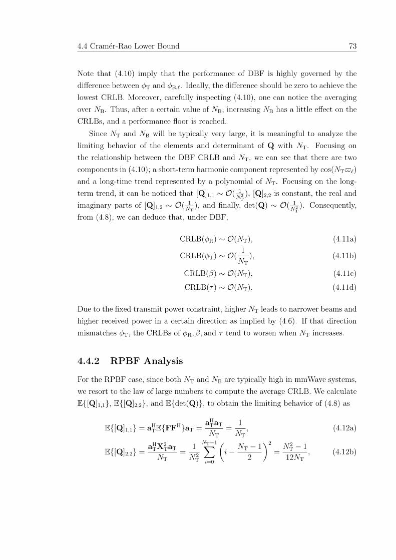
4.4 Cramer-Rao Lower Bound 73
Note that (4.10) imply that the performance of DBF is highly governed by the
difference between φT and φB,`. Ideally, the difference should be zero to achieve the
lowest CRLB. Moreover, carefully inspecting (4.10), one can notice the averaging
over NB. Thus, after a certain value of NB, increasing NB has a little effect on the
CRLBs, and a performance floor is reached.
Since NT and NB will be typically very large, it is meaningful to analyze the
limiting behavior of the elements and determinant of Q with NT. Focusing on
the relationship between the DBF CRLB and NT, we can see that there are two
components in (4.10); a short-term harmonic component represented by cos(NT$`)
and a long-time trend represented by a polynomial of NT. Focusing on the long-
term trend, it can be noticed that [Q]1,1 ∼ O( 1N2
T), [Q]2,2 is constant, the real and
imaginary parts of [Q]1,2 ∼ O( 1NT
), and finally, det(Q) ∼ O( 1N2
T). Consequently,
from (4.8), we can deduce that, under DBF,
CRLB(φR) ∼ O(NT), (4.11a)
CRLB(φT) ∼ O(1
NT
), (4.11b)
CRLB(β) ∼ O(NT), (4.11c)
CRLB(τ) ∼ O(NT). (4.11d)
Due to the fixed transmit power constraint, higher NT leads to narrower beams and
higher received power in a certain direction as implied by (4.6). If that direction
mismatches φT, the CRLBs of φR, β, and τ tend to worsen when NT increases.
4.4.2 RPBF Analysis
For the RPBF case, since both NT and NB are typically high in mmWave systems,
we resort to the law of large numbers to compute the average CRLB. We calculate
E{[Q]1,1}, E{[Q]2,2}, and E{det(Q)}, to obtain the limiting behavior of (4.8) as
E{[Q]1,1} = aHTE{FFH}aT =
aHTaT
NT
=1
NT
, (4.12a)
E{[Q]2,2} =aH
TX2TaT
NT
=1
N2T
NT−1∑
i=0
(i− NT − 1
2
)2
=N2
T − 1
12NT
, (4.12b)
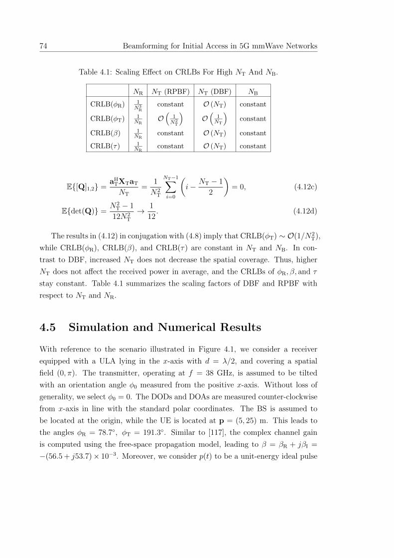
74 Beamforming for Initial Access in 5G mmWave Networks
Table 4.1: Scaling Effect on CRLBs For High NT And NB.
NR NT (RPBF) NT (DBF) NB
CRLB(φR) 1N3
Rconstant O (NT) constant
CRLB(φT) 1NR
O(
1N2
T
)O(
1NT
)constant
CRLB(β) 1NR
constant O (NT) constant
CRLB(τ) 1NR
constant O (NT) constant
E{[Q]1,2} =aH
TXTaT
NT
=1
N2T
NT−1∑
i=0
(i− NT − 1
2
)= 0, (4.12c)
E{det(Q)} =N2
T − 1
12N2T
→ 1
12. (4.12d)
The results in (4.12) in conjugation with (4.8) imply that CRLB(φT) ∼ O(1/N2T),
while CRLB(φR), CRLB(β), and CRLB(τ) are constant in NT and NB. In con-
trast to DBF, increased NT does not decrease the spatial coverage. Thus, higher
NT does not affect the received power in average, and the CRLBs of φR, β, and τ
stay constant. Table 4.1 summarizes the scaling factors of DBF and RPBF with
respect to NT and NR.
4.5 Simulation and Numerical Results
With reference to the scenario illustrated in Figure 4.1, we consider a receiver
equipped with a ULA lying in the x-axis with d = λ/2, and covering a spatial
field (0, π). The transmitter, operating at f = 38 GHz, is assumed to be tilted
with an orientation angle φ0 measured from the positive x-axis. Without loss of
generality, we select φ0 = 0. The DODs and DOAs are measured counter-clockwise
from x-axis in line with the standard polar coordinates. The BS is assumed to
be located at the origin, while the UE is located at p = (5, 25) m. This leads to
the angles φR = 78.7◦, φT = 191.3◦. Similar to [117], the complex channel gain
is computed using the free-space propagation model, leading to β = βR + jβI =
−(56.5 + j53.7)× 10−3. Moreover, we consider p(t) to be a unit-energy ideal pulse
4.5 Simulation and Numerical Results 75
given by
p(t) =1√W
sinc(Wt). (4.13)
Consequently, it follows from Parseval’s theorem that W 2eff = W 2/3, where W =
Rb/2b, and Rb is the bit rate, and b is the number of bits per symbol. We present
the results for 1 Gbps bit rate and 16 QAM transmission, i.e., W = 125 MHz. To
improve the results presentation, we provide the CRLB(τ) in terms of CRLB(d1) =
c2 CRLB(τ). It should be noted that using the values above, the SNR at the given
location can be calculated to be 30.7 dB, which is high enough to guarantee the
tightness of the CRLB of the parameters.
For DBF, the directions are chosen to be equally spaced to cover the region
(0, π), i.e., φB,` = π`NB+1
, 1 ≤ ` ≤ NB. Finally, in the following results, when
referring to RPBF, CRLB means the average CRLB. RPBF plots are obtained by
Monte-Carlo simulation averaged over 1000 iteration.
4.5.1 Effect of NB on the CRLBs of Channel Parameters
Figure 4.3 illustrates the CRLBs of the channel parameters as a function of NB
with NT = 32 and NR = 64. It can be seen that, using RPBF, the CRLB floor is
reached at NB = 18. Also, note that for NB < 10 the average CRLBs of φR and
d1 are less sensitive to NB compared to those of φT, and β. On the other hand,
the CRLB under DBF is non-monotonic. Thus, NB should be carefully chosen for
optimum estimation. However, since in the initial access phase the transmitter has
no information on the direction of transmission, an optimal beam is not guaranteed.
Comparing RPBF with DBF in Figure 4.3, it can be inferred that the RPBF
scheme attains a lower floor at a low NB than the DBF, except when the latter
happens to have a beam close to the receiver direction. To see why the CRLB
floors, notice the averaging effect in (4.10), and the independence of NB in (4.12).
Intuitively, recall that with a fixed NR the receiver beam-width about φR is fixed.
Now, consider the RPBF case shown in Figure 4.2. When NB is small, there is a
limited chance that a random transmit beam will cover φR with a suitable gain, but

76 Beamforming for Initial Access in 5G mmWave Networks
0 10 20 30 40 50 60 70 80 90 100
10−7
10−5
10−3
10−1
101
NB
CRLB
CRLB(φR)CRLB(φT)CRLB(β)CRLB(d1)
Figure 4.3: CRLB of the channel parameters w.r.t NB using RPBF (dashed line)and DBF (solid line) with NR = 64, NT = 32. Directional beams are equally spacedover (0,π)
as NB goes up, this chance enhances and the CRLB starts to decrease. As NB grows
significantly, the resultant beams becomes almost omni-directional and, regardless
of how high NB is, the CRLB becomes fixed. On the other hand, consider the DBF
case in Figure 4.2, where beams have a comb-like shape and the CRLB mainly
depends on the difference between the transmit beams and the DOD. As NB grows
higher, more transmit beams fall within the vicinity of the DOA. However, since
‖f`‖2 = 1/NB, the received power stays fixed, and the CRLB floor is reached.
4.5.2 Effect of NR on the CRLBs of Channel Parameters
The CRLBs of the channel parameters as function of NR are provided in Figure
4.4. In both schemes, CRLBs of φT, β, and τ decrease as 1/NR. On the other
hand, CRLB of φR decreases by three orders of magnitude, when NR increases by
one order of magnitude. This is in line with the theoretical expressions in (4.8).
Finally, as is the case with respect to NT, these results confirm the conclusion made
using Figure 4.3 that RPBF provides better bounds than DBF does when NB is
fixed.

4.5 Simulation and Numerical Results 77
20 40 60 80 100 120 140 160 180 20010−8
10−7
10−6
10−5
10−4
10−3
10−2
NR
CRLB
CRLB(φR)CRLB(φT)CRLB(β)CRLB(d1)
Figure 4.4: CRLB w.r.t NR using RPBF (dashed line) and DBF (solid line) withNB = 18, NT = 32. Directional beams are equally spaced over (0,π)
4.5.3 Effect of NT on the CRLB
Figure 4.5 illustrates the results of investigating the CRLB in terms of NT. Con-
sidering DBF, it is hard to draw any conclusion for scaling factors in terms of NT
due to the high non-linearity observed and represented by (4.10). However, there is
an average trend that can be seen, as discussed in Section 4.4, whereby CRLB(φT)
decreases with 1/N2T while the other CRLBs increase with NT. As for RPBF, it can
be seen from Figure 4.5 that only the estimation of φT improves when increasing
NT. Note that due to the power normalization discussed in Section 4.2, the CRLBs
of β and φR are not affected by an increased NT.
4.5.4 Summary of Results
From Figures 4.3 – 4.5, it can be inferred that RPBF outperforms DBF in terms
of the CRLBs of the channel parameters, except in some cases shown in Figure
4.3, where a few NB choices can result in a better DBF performance. Note that in
these cases a beam or more are close enough to the receiver direction, hence the
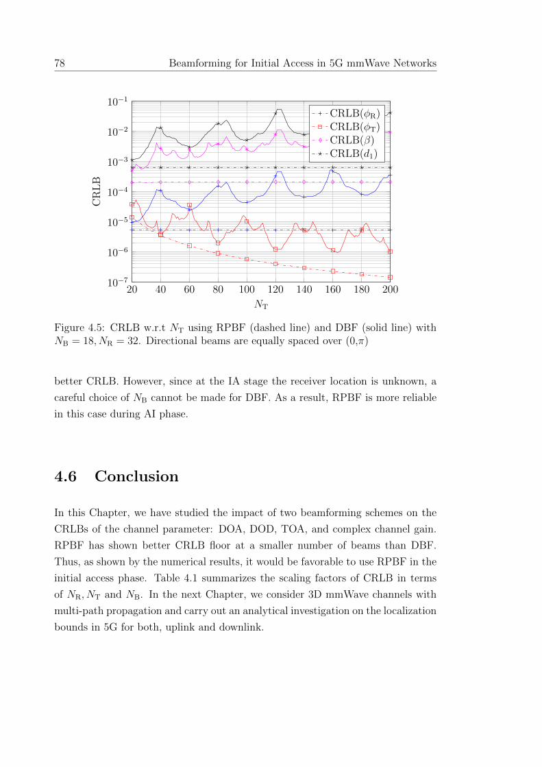
78 Beamforming for Initial Access in 5G mmWave Networks
20 40 60 80 100 120 140 160 180 20010−7
10−6
10−5
10−4
10−3
10−2
10−1
NT
CRLB
CRLB(φR)CRLB(φT)CRLB(β)CRLB(d1)
Figure 4.5: CRLB w.r.t NT using RPBF (dashed line) and DBF (solid line) withNB = 18, NR = 32. Directional beams are equally spaced over (0,π)
better CRLB. However, since at the IA stage the receiver location is unknown, a
careful choice of NB cannot be made for DBF. As a result, RPBF is more reliable
in this case during AI phase.
4.6 Conclusion
In this Chapter, we have studied the impact of two beamforming schemes on the
CRLBs of the channel parameter: DOA, DOD, TOA, and complex channel gain.
RPBF has shown better CRLB floor at a smaller number of beams than DBF.
Thus, as shown by the numerical results, it would be favorable to use RPBF in the
initial access phase. Table 4.1 summarizes the scaling factors of CRLB in terms
of NR, NT and NB. In the next Chapter, we consider 3D mmWave channels with
multi-path propagation and carry out an analytical investigation on the localization
bounds in 5G for both, uplink and downlink.

4.6 Conclusion 79
Publications Resulted from This Chapter
� Z. Abu-Shaban,H. Wymeersch, X. Zhou, G. Seco-Granados, T. Abhaya-
pala “Random-Phase Beamforming for Initial Access in the Millimeter-Wave
Cellular Networks” in 2016 IEEE Global Communications Conf. (GLOBE-
COM), Washington, DC, pp. 1-6, Dec 2016.


Chapter 5
Uplink and Downlink 3D
Localization Error Bounds in 5G
mmWave Systems
Overview: Location-aware communication systems are expected to play a pivotal
part in the next generation of mobile communication networks. Therefore, there is
a need to understand the localization limits in these networks, particularly, using
mmWave. Towards that, we address the uplink and downlink localization limits in
terms of 3D position and orientation error bounds for mmWave multipath channels.
We also carry out a detailed analysis of the dependence of the bounds on different
system parameters. Our key findings indicate that the uplink and downlink behave
differently in two distinct ways. First of all, the error bounds have different scaling
factors with respect to the number of antennas in the uplink and downlink. Sec-
ondly, uplink localization is sensitive to the orientation angle of the UE, whereas
downlink is not. Moreover, in the considered outdoor scenarios, the non-line-of-
sight paths generally improve localization when a line-of-sight path exists. Finally,
our numerical results show that mmWave systems are capable of localizing a UE
with sub-meter position error, and sub-degree orientation error.
81

82 Uplink and Downlink 3D Localization Error Bounds in 5G mmWave Systems
5.1 Introduction
Having considered the initial network access problem in the previous Chapter, we
now focus on UE localization in mmWave location-aided systems.
Location-aided systems are expected to have a wide range of applications in 5G
mmWave communication [26], whether for vehicular communications [118], assisted
living applications [68], or to support the communication robustness and effective-
ness in different aspects such as resource allocation [119], beamforming [33, 71],
and pilot assignment [34]. Therefore, the study of positioning in 5G mmWave
systems becomes especially imperative. Due to the use of directional beamform-
ing in mmWave, in addition to the UE position also the UE orientation plays an
important role in location-aided systems.
Conventionally position information is obtained by GPS, though this has sev-
eral limitations. Most importantly, GPS suffers from degraded performance in
outdoor rich-scattering scenarios and urban canyons, and may fail to provide a po-
sition fix for indoor scenarios. Even in good conditions, GPS positioning accuracy
ranges between 1–5 meters. To address these limitations, there has been intense
research on competing radio-based localization technologies. To understand the
fundamental behavior of any technology, the CRLB or related bounds can be used.
As discussed in Section 2.2.3, the CRLB provides a lower bound on the variance
of an unbiased estimator of a certain parameter. The square-root of the CRLB of
the position and the orientation are termed the position error bound (PEB), and
the orientation error bound (OEB), respectively. PEB and OEB can be computed
indirectly by transforming the bounds of the channel parameters, namely: DOA,
DOD, and TOA.
For conventional MIMO systems, the bounds of the 2D channel parameters are
derived in [120], based on received digital signals and uniform linear arrays (ULA),
while bounds are derived in [121] based on 3D channel matrix with no transmit
beamforming. It was found that having more transmit and receive antennas is ben-
eficial for estimating the DOA and DOD. In both [120, 121] beamforming was not
considered. The bounds on the channel parameters can be transformed into PEB
and OEB as in [84,122–124] that considered 2D cooperative wideband localization,
highlighting the benefit of large bandwidths.

5.1 Introduction 83
MmWave communication combines large antenna arrays with large bandwidths,
and should be promising for localization, then. In [125], PEB and OEB for 2D
mmWave downlink localization using ULA are reported, while [126] considers 2D
uplink multi-anchor localization. Furthermore, for indoor scenarios, PEB and OEB
are analyzed in [127] for 3D mmWave uplink localization with a single beam whose
direction is assumed to be known. Although multipath channels are considered in
[125–127], the difference between the uplink and downlink for 3D and 2D with large
number of antennas and analog transmit beamforming is yet to be investigated.
In this Chapter, we consider 3D mmWave localization problem for both the
uplink and downlink under multipath conditions, and derive and analyze the PEB
and OEB using multi-beam directional beamforming with arbitrary array geometry.
By their nature, these bounds are theoretical, and serve as benchmarks to assess
location estimation techniques, as well as being a feasibility study to see how well
the location and orientation can be potentially estimated. We derive these bounds
by transforming the Fisher information matrix (FIM) of the channel parameters
into the FIM of location parameters. We stress that although the FIM of the
channel parameters is structured similarly in the uplink and downlink, this is untrue
for the location parameters FIM, which is obtained by transforming the FIM of the
channel parameters. Using procedure similar to the one introduced in Section 2.2.4,
this transformation is different in the uplink and downlink, and leads to different
PEB and OEB. The contributions of this Chapter are summarized as follows:
� Based on the low-scattering sparse nature of the mmWave channel and the
resulting geometrical model, we show that, under some conditions, the mul-
tipath parameter estimation can be reduced to a problem of multiple single-
path estimation. We refer to this reduction as the approximate approach.
These conditions are highly relevant in mmWave due to channel sparsity, high
number of receive and transmit antennas, and the very large bandwidth.
� We derive the single-path CRLB of the channel parameters in a closed-form
for arbitrary geometry, and show how these bounds are related to the PEB
and OEB bounds. We also propose closed-form expressions of PEB and OEB
for 3D and 2D LOS localization. Although our derivation is for an arbitrary
array geometry, we specify the results for URA and ULA.
84 Uplink and Downlink 3D Localization Error Bounds in 5G mmWave Systems
� We derive the PEB and OEB for general uplink and downlink localization,
based on exact and approximate approaches, and show the asymmetry be-
tween uplink and downlink via both analytical scaling results and numerical
simulations with a URA.
The rest of this Chapter is organized as follows. Section 5.2 presents the problem
statement. Then, in Section 5.3, we derive the FIM of the channel parameters
in a general setup of arbitrary arrays for 3D localization.The transformation of
the channel parameters FIM into PEB and OEB is detailed in Section 5.4. The
simulation results and the related insights are provided in Section 5.5. Finally, the
conclusions are reported in Section 5.6.
5.2 Problem Formulation
5.2.1 System Geometry
By extending the 2D system geometry considered in Chapter 4, to the general case
of 3D, we consider a BS equipped with an array of NBS antennas arranged in an
arbitrary but known geometry whose centroid, i.e., geometric center, is located
at the origin (O), and orientation angle is oBS = [0, 0]T. On the other hand,
the centroid of the UE is located at an unknown position p = [px, py, pz]T and
equipped with a second array of NUE antennas arranged in an arbitrary but known
geometry with an unknown orientation o = [θ0, φ0]T, aligning the UE with the
rotated axes x′, y′ and z′. An example with URAs is depicted in Figure 5.1. φ0 is
defined as the rotation around the z-axis, while θ0 is defined as the rotation around
the −x′-axis. Thus, the UE array elements locations is obtained using a rotation
matrix R(θ0, φ0) derived in (5.35). Considering two orientation angles is highly
relevant in applications such as vehicular communication and robotics, where the
UE turns left and right, or goes up or down hills, without rotating the vehicle axis.
We further assume that there are M ≥ 1 paths between BS and UE, where the
first path is LOS, while with the other M − 1 paths are associated with clusters
located at qm = [qm,x, qm,y, qm,z]T, 2 ≤ m ≤ M . These clusters can reflectors
or scatterers. Due to the mmWave propagation characteristics, the number of
paths is small [62] and correspond to single-bounce reflections [117,125]. In fact, it

5.2 Problem Formulation 85
x
y
z
x y
z
x y
z
(xBS,n, yBS,n, zBS,n)
(xUE,n, yUE,n, zUE,n)
BS:NBS
O
NUEUE:
p
q2
coordinate system
θ
φ
ρ
d2,2
d2,1
dm,1
qM
dm,2
d1
......
φ0
θ0
x′
y′
z′
Figure 5.1: An example scenario composed of a URA of NUE = NBS = 81 antennas,and M paths. We use the spherical coordinate system highlighted in the top rightcorner. The axes rotated by orientation angles (θ0, φ0) are labeled x′, y′, z′.
was experimentally observed in [66] that the average value of M under mmWave
propagation in an urban environment in New York City is 2 to 3 paths with a
maximum of 4 paths present during measurement. This consequently resulted in
modeling M by a Poisson mass function whose average is 1.8 and 1.9 at 28 GHz,
and 73 GHz, respectively. Thus, the channel can be considered spatially sparse,
and the parameters of different paths are assumed to be distinct, i.e., we assume
unique DOAs, DODs, and TOA.
5.2.2 Channel Model
Denote the mth DOD and DOA by (θT,m, φT,m) and (θR,m, φR,m), 1 ≤ m ≤ M ,
respectively, where the related unit-norm array response vectors are given by [58]
aT,m(θT,m, φT,m) ,1√NT
e−j∆TTk(θT,m,φT,m), ∈ CNT (5.1)
86 Uplink and Downlink 3D Localization Error Bounds in 5G mmWave Systems
aR,m(θR,m, φR,m) ,1√NR
e−j∆TRk(θR,m,φR,m), ∈ CNR (5.2)
where k(θ, φ), λ, and ∆R ∈ R3×NR , are as defined in Section 2.1.1, while NR is the
number of receiving antennas. NT, and ∆T are defined similarly1. We drop the
angle parameters from the notation of aT,m, and aR,m.
Assuming synchronization2, and denoting the TOA of the mth path by τm, the
channel can be expressed3 as
H(t) =M∑
m=1
Hmδ(t− τm), (5.3)
From Figure 5.1, τm = dm/c, where dm = dm,1 + dm,2, for m > 1 and
Hm ,√NRNTβmaR,maH
T,m ∈ CNR×NT , (5.4)
where βm is the complex gain of the mth path. Finally, we define the following
θR , [θR,1, θR,2, ..., θR,M ]T,
θT , [θT,1, θT,2, ..., θT,M ]T,
β , [β1, β2, ..., βM ]T,
φR , [φR,1, φR,2, ..., φR,M ]T,
φT , [φT,1, φT,2, ..., φT,M ]T,
τ , [τ1, τ2, ..., τM ]T.
5.2.3 Transceiver Model
The transmitter sends a signal x(t) =√EtFs(t), as defined in (4.4). Here, we only
consider directional beamforming such that F , [f1, f2, ...fNB], where
f` =1√NB
aT,`(θ`, φ`), 1 ≤ ` ≤ NB (5.5)
1The subscripts T and R refer to the transmit and receive sides, respectively, regardless ofusing the uplink or downlink. On the other hand, when the notation is unique to the base stationor the user equipment, we use the subscript BS and UE.
2We rely on the commonly used synchronization assumption e.g., [68], [120], [84,122–124], [126],to gain fundamental understanding. We, however, realize that in practice synchronization errorsmust be accounted for in protocols and algorithms. This can be done by, e.g., a two-way protocolor a joint localization and synchronization approach, which is addressed in Chapter 6.
3We use a narrow-band array model, so that Amax � c/W , where Amax is maximum arrayaperture, c is speed of light, and W is the system bandwidth [58].

5.3 FIM of The Channel Parameters 87
The received signal observed at the input of the receive beamformer is given by
r(t) ,M∑
m=1
√EtHmFs(t− τm) + n(t), t ∈ [0, To], (5.6)
where n(t) , [n1(t), n2(t), ..., nNR(t)]T ∈ CNR is zero-mean white Gaussian noise
with PSD N0. Similar to [128, 129], we assume that a low-noise amplifier and
a passband filter are attached to each receive antenna. While this may seem a
restrictive assumption, it will allow us to derive the PEB and OEB, which are
fundamental lower bounds irrespective of the type of processing performed at the
receiver, such as receive beamforming.
5.2.4 3D Localization Problem
Our objective is to derive the UE PEB and OEB, based on the observed signal,
r(t), for both the uplink and downlink. We achieve this in two steps: firstly, we
derive bounds on the channel parameters, namely, direction of arrival, (θR,φR),
direction of departure, (θT,φT), time of arrival τ , and paths gains, β. Secondly,
we transform these bounds into the position domain.
5.3 FIM of The Channel Parameters
We first derive exact expressions for the entries of the FIM. Then, we determine
the conditions under which the individual paths can be considered orthogonal.
Subsequently, we provide closed-form expressions of the CRLB for the single-path
case for 3D and 2D localization.
5.3.1 Exact Expression
Let us define the parameter vector
ϕ , [θTR,θ
TT,φ
TR,φ
TT, τ
T,βTR,β
TI ]T, (5.7)

88 Uplink and Downlink 3D Localization Error Bounds in 5G mmWave Systems
where βR , <{β}, and βI , ={β} are the real and imaginary parts of β, re-
spectively, and denote the uth element in ϕ by ϕu. Then, the corresponding FIM,
partitioned into M ×M submatrices, is structured as
Jϕ ,
JθRθR JθRθT · · · JθRβI
JTθRθT
. . . · · · ...... · · · . . .
...
JTθRτ
· · · · · · JβIβI
, (5.8)
where, due to the additive white Gaussian noise [81],
[Jϕ]u,v ,1
N0
∫ To
0
<{∂µH
ϕ(t)
∂ϕu
∂µϕ(t)
∂ϕv
}dt, (5.9)
where µϕ(t) is the noiseless part of received signal in (5.6).
µϕ(t) ,√NRNTEt
M∑
m=1
βmaR,maHT,mFs(t− τm). (5.10)
We now introduce the following matrices to simplify the notation
B , diag(β) (5.11a)
AR , [aR,1, aR,2, ..., aM ], (5.11b)
KR,m , diag
(∂
∂θR,m
∆TRk(θR,m, φR,m)
), (5.11c)
PR,m , diag
(∂
∂φR,m
∆TRk(θR,m, φR,m)
), (5.11d)
KR , [KR,1aR,1, KR,2aR,2, ..., KR,NRaR,NR
], (5.11e)
PR , [PR,1aR,1, PR,2aR,2, ..., PR,NRaR,NR
], (5.11f)
with similar expressions obtained by replacing “R” with “T”. It is shown in Ap-
pendix B that each submatrix in (5.8) is of the form
Jx,x′ = <{(RX factor)� (TX factor)� (signal factor)} , (5.12)

5.3 FIM of The Channel Parameters 89
where � denotes the Hadamard product, the RX factor relates to the receiver
array, the TX factor relates to the transmitter array and beamforming, and the
signal factor relates to the pilot signals. The RX factor is a product of the ma-
trices {ARB,KRB,PRB}, while the TX part is a product of similar matrices
{FHAT,FHKT,F
HPT}, associated with the transmitter as well as F. Under the
assumption of i.i.d. symbols, the signal factor depends on
[Ri]uv ,∫ W/2
−W/2(2πf)i|P (f)|2e−j2πf∆τuvdf, (5.13)
in which ∆τuv , τv − τu, i ∈ {0, 1, 2}. The signal factor in (5.13) represents
the correlation between different paths obtained in the frequency domain using
Parseval’s theorem. See (B.8), (B.11) and (B.12).
For instance, defining the signal-to-noise ratio (SNR) as
γ ,NRNTNsEt
N0
, (5.14)
it can be verified that
JθRθR = γ<{
(BHKHRKRB)� (AH
TFFHAT)T �R0
}, (5.15)
The rest of the FIM entries in (5.8) are listed in Appendix B, and all exhibit the
structure in (5.12). Observe that the FIMs in (5.8) scale linearly with SNR, which
means that the CRLB decreases as SNR increases.
5.3.2 Approximate FIM of the Channel Parameters
The exact FIMs presented in Section 5.3.1 provide the exact CRLB of the channel
parameters. However, under some circumstances, it is possible to simplify this
computation by reducing the submatrices of the FIMs to either diagonal or zero
matrices, by exploiting the structure in (5.12). Inspired by [130], we start by
introducing the following definition.
Definition 5.1 Given a square matrix A(κ) that can be decomposed into a diago-
nal matrix D(κ) 6= 0 plus a hollow matrix E(κ) 6= 0, then A(κ) = D(κ) + E(κ) is
90 Uplink and Downlink 3D Localization Error Bounds in 5G mmWave Systems
almost diagonal (AD) for any parameter κ if
limκ→∞
δ(A, κ) , limκ→∞
‖E(κ)‖F
‖D(κ)‖F
= 0. (5.16)
We now use Definition 5.1 to inspect the factors in (5.12), and understand the
behavior under typical mmWave conditions, i.e., large transmit and receive arrays
and large system bandwidth.
� Factor 1 – Receiver Side: For a large number of receive antennas, the power
received from a direction (θR,u, φR,u) via a steering vector in the direction
(θR,v, φR,v) is very small, i.e., ‖aHR,uaR,v‖ � ‖aR,u‖2, u 6= v, when the DOAs of
the different paths are distinct. Thus, limNR→∞ δ(AHRAR, NR) = 0. Similarly,
considering the exponential form of aR,m and that KR,m, PR,m are diagonal,
limNR→∞
δ(KHRKR, NR) = lim
NR→∞δ(PH
RPR, NR), (5.17a)
= limNR→∞
δ(KHRPR, NR) = 0. (5.17b)
On the other hand, using the facts that the BS centroid is at the origin,
then for uplink Tr(KR,m) =∑NR
n=0∂∂θR
∆TRk =
(∑NR
n=0 ∆TR
)∂∂θR
k = 0, and
similarly, Tr(PR,m) = 0, and that the UE centroid is at p, then for down-
link Tr(KR,m) = pT ∂∂θm
k, Tr(PR,m) = pT ∂∂φm
k. Moreover, Noting that
[KHRAR]m,m = Tr(KR,m)/NR, then, for both uplink or downlink,
limNR→∞
KHRAR = lim
NR→∞PH
RAR = 0M×M . (5.18)
where 0M×M is an M ×M matrix of zeros.
� Factor 2 – Transmitter Side: The transmitter side contributes to the FIM
in (5.15) by AHTFFHAT. Recalling that [AH
TFFHAT]u,v = aHT,uFFHaT,v, the
right-hand side term can be interpreted as the spatial cross-correlation be-
tween the uth and the vth DODs. So, considering directional beamforming,
as NT increases, the beams become narrower, leading to
limNT→∞
aHT,uFFHaT,v ≈ 0 u 6= v. (5.19)

5.3 FIM of The Channel Parameters 91
Moreover, for extremely narrow beams, the likelihood of covering the vth
DOD is almost zero,
limNT→∞
aHT,vFFHaT,v = lim
NT→∞‖FHaT,v‖2 ≈ 0. (5.20)
In this extreme case, AHTFFHAT ≈ 0, which implies the whole FIM is zero.
However, since (5.19) approaches 0 faster than (5.20), the transmission over
directional beamforming should be restricted to NT <∞. That said, there
are cases where (5.20) does not hold and AHTFFHAT is AD, e.g., when using
random beamforming. By inspection, a similar statement can be made for
(PHTFFHPT)T, (KH
TFFHKT)T, and (PHTFFHKT)T.
� Factor 3: Multipath Cross-Correlation: It can be shown that the cross-
correlation functions in (5.13) are even in ∆τuv for i = 0, 2 and have maxima
on their diagonals. These maxima are constant with values 1 and 4π2W 2eff ,
respectively, where W 2eff is as defined in (4.9b). Moreover,
limW→∞
δ(R0,W ) = 0, (5.21a)
limW→∞
δ(R2,W ) = 0. (5.21b)
Regarding R1, we note that for any W , diag(R1) = 0M so that R1 is a hollow
matrix, with limW→∞R1 = 0M×M . So, in effect, the paths overlapping in
time is negligible, which is consistent with [131] and [132].
In combination, given the Hadamard product structure of (5.12), we find that
under typical mmWave conditions, due to the combined effect of large values of NR,
and W , some submatrices of the FIM in (5.8) are AD, while the others are almost
zero as shown in Figure 5.2 (left). This effect relates to the fact that paths can be
resolved in either direction of arrival or delay domain, both of which reinforce each
other in mmWave. In other words, it is sufficient to have NR →∞ or W →∞ in
order for the paths to be orthogonal. However, as it is customary to have a very
large antenna array at the base station, it is reasonable to assume that paths are
always orthogonal. Re-ordering the parameters, grouping them path by path, we
obtain the block diagonal FIM in Figure 5.2 (right).
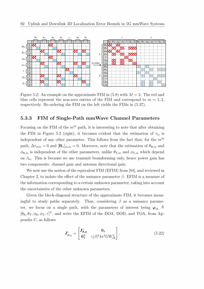
92 Uplink and Downlink 3D Localization Error Bounds in 5G mmWave Systems
re-order
θR︷ ︸︸ ︷1 2
θT︷ ︸︸ ︷1 2
φR︷ ︸︸ ︷1 2
φT︷ ︸︸ ︷1 2
τ︷ ︸︸ ︷1 2
βR︷ ︸︸ ︷1 2
βI︷ ︸︸ ︷1 2
1︷ ︸︸ ︷θR, θT, φR, φT, τ, βR, βI
2︷ ︸︸ ︷θR, θT, φR, φT, τ, βR, βI
θRθTφR
φT
τβRβIθRθTφR
φT
τβRβI
︷︸︸
︷︷
︸︸︷
1
2
12121212121212
︷︸︸︷
︷︸︸︷
︷︸︸︷
︷︸︸︷
︷︸︸︷
︷︸︸︷
︷︸︸︷
θR
θT
φR
φT
τ
βR
βI
Figure 5.2: An example on the approximate FIM in (5.8) with M = 2. The red andblue cells represent the non-zero entries of the FIM and correspond to m = 1, 2,respectively. Re-ordering the FIM on the left yields the FIMs in (5.37).
5.3.3 FIM of Single-Path mmWave Channel Parameters
Focusing on the FIM of the mth path, it is interesting to note that after obtaining
the FIM in Figure 5.2 (right), it becomes evident that the estimation of τm is
independent of any other parameter. This follows from the fact that, for the mth
path, ∆τmm = 0 and [R1]m,m = 0. Moreover, note that the estimation of θR,m and
φR,m is independent of the other parameters, unlike θT,m and φT,m which depend
on βm. This is because we use transmit beamforming only, hence power gain has
two components: channel gain and antenna directional gain.
We now use the notion of the equivalent FIM (EFIM) from [84], and reviewed in
Chapter 2, to isolate the effect of the nuisance parameter β. EFIM is a measure of
the information corresponding to a certain unknown parameter, taking into account
the uncertainties of the other unknown parameters.
Given the block-diagonal structure of the approximate FIM, it becomes mean-
ingful to study paths separately. Thus, considering β as a nuisance parame-
ter, we focus on a single path, with the parameters of interest being ϕch ,
[θR, θT, φR, φT, τ ]T, and write the EFIM of the DOA, DOD, and TOA, from Ap-
pendix C, as follows
Jeϕch
=
[Jeθ,φ 04
0T4 γ|β|24π2GW 2
eff
], (5.22)

5.3 FIM of The Channel Parameters 93
where
Jeθ,φ = γ|β|2
RθG 0 Xθ,φG 0
0 LθG
0Yθ,φG
Xθ,φG 0 RφG 0
0Yθ,φG
0LφG
, (5.23)
in which
Rθ , aHRK2
RaR,
Rφ , aHRP2
RaR,
Vθ , aHTKTFFHaT,
Vφ , aHTPTFFHaT.
Lθ , GTθ − |Vθ|2,Lφ , GTφ − |Vφ|2,Tθ , aH
TKTFFHKTaT,
Tφ , aHTPTFFHPTaT,
G , aHTFFHaT,
Xθ,φ , aHRKRPRaR,
Yθ,φ , GY ′θ,φ −<{VφV ∗θ },Y ′θ,φ , <{aH
TPTFFHKTaT},
Note that G denotes the transmit array gain in a direction θT, while Rθ, Rφ, Tθ,
and Tφ are the information contents related to the spatial aspects of the received
signal and correspond to θR, φR, θT, and φT, excluding the SNR, i.e., the integrands
in (5.9). Similarly, Vθ, Vφ, Xθ,φ, and Y ′θ,φ respectively represent the mutual spatial
information between θT and β, φT and β, θR and φR, and θT and φT. Consequently,
Lθ and Lφ represent the equivalent Fisher spatial information of θT and φT, respec-
tively, after removing the dependence on β. Finally, Yθ,φ denotes the equivalent
mutual information of θT and φT, after removing the dependence on β.
The CRLB of the channel parameters for arbitrary array geometries is provided
below.
Proposition 5.1 Based on the FIM in (5.22), the CRLBs of the DOA, DOD and
TOA are given by
CRLB (θR)=1
γ|β|2 G(Rθ −
X2θ,φ
Rφ
) =Rφ
γζ1|β|2G, (5.24a)
CRLB (φR)=1
γ|β|2 G(Rφ −
X2θ,φ
Rθ
) =Rθ
γζ1|β|2G, (5.24b)
CRLB (θT)=G
γ|β|2(Lθ −
Y 2θ,φ
Lφ
) =GLφγζ2|β|2
, (5.24c)

94 Uplink and Downlink 3D Localization Error Bounds in 5G mmWave Systems
CRLB (φT)=G
γ|β|2(Lφ −
Y 2θ,φ
Lθ
) =GLθγζ2|β|2
, (5.24d)
CRLB(τ) =1
(4π2W 2eff)(γ|β|2G)
. (5.24e)
where ζ1 = RθRφ −X2θ,φ, and ζ2 = LθLφ − Y 2
θ,φ.
Proof
See Appendix C.1.
Note that the CRLBs in (5.24) consist of two components: Firstly, there is an
SNR component represented by γ|β|2 G for the receiver angles, and by G/(γ|β|2) for
the transmitter angles. This component is inversely proportional to the CRLBs,
which means with higher SNR, the CRLBs of the channel parameters decrease.
Secondly, there is a spatial information part in the parentheses containing the
equivalent information after removing the dependence on the other parameter.
Proposition 5.2 For 2D localization, when the UE and BS are located in the xy-
plane, θR = θT = π/2
CRLB(φR) =1
γ|β|2RφG, (5.25a)
CRLB(φT) =G
γ|β|2Lφ, (5.25b)
while CRLB(τ) is unchanged.
Proof
See Appendix C.2.
Recall that θR = θT are known and can be removed from ϕch, leading to (5.25).
Moreover, Note that these expressions can be viewed as special cases of Proposition
5.1, by ignoring the terms relating to the coupling between θ and φ. Appendix C.3
provides details on the computation of the FIM and CRLB for URA and ULA as
special cases.

5.4 FIM of the Location Parameters 95
5.4 FIM of the Location Parameters
In the preceding sections, we have seen how the FIM of the multipath channel
parameters can be approximated by multiple single-path FIMs. We have also
derived the single-path FIM for different settings. In this section, we derive the PEB
and the OEB by applying a transformation [81] to the EFIM of DOA, DOD, and
TOA, computed from (5.8), to obtain the exact FIM of position and orientation.
We also transform Jϕch, defined in (5.22), to obtain the approximate one.
5.4.1 PEB and OEB: Exact Approach
General Formulation
Before proceeding further, we state the following theorem.
Theorem 5.1 (Equivalence Theorem) The FIM of position and orientation
obtained by transforming the EFIM of the directions of arrival and departure, and
the time of arrival is equivalent to the EFIM of position and orientation obtained
by direct transformation of the FIM of the directions of arrival, departure, time of
arrival and other nuisance parameter.
Proof
See Appendix D.1.
This means that instead of transforming the FIM of all the channel parameters
(useful and nuisance), and then computing the EFIM of p and o, we can simplify
that by only transforming the EFIM of the useful channel parameters (DOAs,
DODs, TOAs).
In this section, we derive the PEB and OEB based on the EFIM of the multipath
channel parameters of interest ϕCH , [θT,φT, τT]T. We do so by first transforming
JeϕCH
to a FIM of the location parameters ϕL , [oT,pT,qT]T, where
θ ,[θT
R,θTT
]T, (5.26a)
φ ,[φT
R,φTT
]T, (5.26b)
q ,[qT
2 ,qT3 , · · · ,qT
M
]T. (5.26c)

96 Uplink and Downlink 3D Localization Error Bounds in 5G mmWave Systems
Towards that, we write
JϕL, ΥJe
ϕCHΥT ,
[Jop Jop,q
JTop,q Jq
], (5.27)
where Jop ∈ R5×5, Jq ∈ R3(M−1)×3(M−1) and
Υ =∂ϕT
CH
∂ϕL
=
∂θT
∂o∂φT
∂o∂τT
∂o∂θT
∂p∂φT
∂p∂τT
∂p∂θT
∂q∂φT
∂q∂τT
∂q
. (5.28)
Consequently, the EFIM of p and o is found via Schur’s complement as
Jeo,p = Jop − Jop,qJ−1
q JTop,q. (5.29)
Finally, the PEB and OEB are given by the square roots of the squared-PEB
(SPEB) and squared-OEB (SOEB) defined in the following.
Definition 5.2 For the equivalent Fisher information matrix of the position and
the orientation, Jeo,p ∈ R5×5, the SOEB and SPEB are defined as:
SOEB =[(Je
o,p)−1]
1,1+[(Je
o,p)−1]
2,2, (5.30a)
SPEB =[(Je
o,p)−1]
3,3+[(Je
o,p)−1]
4,4+[(Je
o,p)−1]
5,5. (5.30b)
Transformation for Uplink and Downlink
The relationships governing the UE position and orientation with the BS and UE
angles are different. Therefore, unlike Jϕ, the structure of Υ and, effectively, Jeo,p,
depends on whether the uplink or downlink is used for signal transmission. For
this reason, we switch to the explicit notation with the subscripts BS and UE,
θ =
[θT
BS,θTUE
]T, uplink
[θT
UE,θTBS
]T, downlink
, (5.31a)
φ =
[φT
BS,φTUE
]T, uplink
[φT
UE,φTBS
]T, downlink.
(5.31b)

5.4 FIM of the Location Parameters 97
BS
UE
(0, 0)x
yx
y
p
x′y′
φ0φUE
φBS BS
UE
−px
yx
y
(0, 0)
x′y′
φ0φUE
φBS
BS
UE
−p
p′
φ0x
y
x′
y′
(0, 0)x
y
φ0
φUE
Original coordinate system Step 1: Shift the origin to p Step 2: Rotate the coordinate system by −φ0
Figure 5.3: Two-step derivation of the UE angle in 2D. It is easy to see thatφUE = tan−1
(p′y/p
′x
), where p′ = −Rz(−φ0)p.
where φBS and θBS denote the vectors of the azimuth and elevation angles at the
BS, and φUE and θUE are the azimuth and elevation angles at the UE.
Starting with LOS and using the spherical coordinates, it can be seen from
Fig. 5.1 that
θBS,1 = cos−1 (pz/‖p‖) , (5.32a)
φBS,1 = tan−1 (py/px) , (5.32b)
τ1 = ‖p‖/c. (5.32c)
However, the relationship of the UE angles with the position and orientation angles
are not as obvious. Therefore, we resort to the two-step procedure illustrated in
Fig. 5.3 for 2D, but easily extensible to 3D. In the first step, we shift the coordinate
system origin to the UE, hence, the BS is shifted to −p. In the second step, the
coordinate system is rotated in the negative direction of the orientation angle (φ0).
Consequently, the BS location is also rotated, and the UE angles are then taken as
the spherical coordinates of the new BS location. Mathematically, this location is
given by p′ = −Rz(−φ0)p = −R−1z (φ0)p, where Rz(φ0) is the rotation matrix in
the direction φ0 around the z-axis. Generalizing this result to the 3D case yields,
p′ = −R−1(θ0, φ0)p. (5.33)
Consequently, defining p′ , [p′x, p′y, p′z]
T and noting that ‖p‖ = ‖p′‖, we write
θUE,1 = cos−1 (p′z/‖p‖) , (5.34a)

98 Uplink and Downlink 3D Localization Error Bounds in 5G mmWave Systems
φUE,1 = tan−1(p′y/p
′x
). (5.34b)
With the right-hand rule in mind, the rotation considered in this paper (See
Fig. 5.1) is a rotation by φ0 around the z-axis, followed by another rotation by
θ0 around the negative x′-axis. Thus, the rotation matrix is given by [133]
R(θ0, φ0) = Rz(φ0)R−x′(θ0),
=
cosφ0 − sinφ0 cos θ0 − sinφ0 sin θ0
sinφ0 cosφ0 cos θ0 cosφ0 sin θ0
0 − sin θ0 cos θ0
. (5.35)
Note that R(θ0, φ0) is orthogonal and hence satisfies R−1(θ0, φ0) = RT(θ0, φ0).
Next, considering the NLOS paths (2 ≤ m ≤M) and using the same procedure,
the following relations can be obtained
θUE,m = cos−1(w′m,z/‖wm‖
), (5.36a)
φUE,m = tan−1(w′m,y/w
′m,x
), (5.36b)
θBS,m = cos−1 (qm,z/‖qm‖) , (5.36c)
φBS,m = tan−1 (qm,y/qm,x) , (5.36d)
τm = (‖qm‖+ ‖wm‖) /c, (5.36e)
wm = p− qm, (5.36f)
where w′m , [w′m,x, w′m,y, w
′m,z]
T = −RT(θ0, φ0)wm. Based on (5.32), (5.34), and
(5.36), the non-zero elements of Υ are listed in Appendix E.
5.4.2 PEB and OEB: Approximate Approach
In Section 5.3.2, it was concluded that, under certain conditions, the multiple
paths arriving at the receiver can be treated as non-interfering paths carrying
independent information. Thus, we can write the total EFIM of position and
orientation as a sum of the individual EFIMs obtained by transforming the FIM
of useful channel parameters (DOAs, DODs,TOAs), and apply Theorem 5.1 in the
following proposition.
5.4 FIM of the Location Parameters 99
Proposition 5.3 Define the vector of useful channel parameters of the mth path by
ϕ(m)ch , [θR,m, θT,m, φR,m, φT,m, τm]T, and let J
(m)ϕs be the FIM of all the parameters of
mth path, such that ϕs(m) , [θR,m, θT,m, φR,m, φT,m, τm, βR,m, βI,m]. Then we write
J(m)ϕs,
[J
(m)ch J
(m)ch,β
J(m)T
ch,β J(m)ββ
], (5.37)
where J(m)ch ∈ R5×5 is the FIM of ϕ
(m)ch , J
(m)ββ ∈ R2×2 is the FIM of βR,m and βI,m,
and J(m)ch,β ∈ R5×2 is the mutual information matrix of ϕ
(m)ch and β. Moreover,
denote the EFIM of the mth DOA, DOD, and TOA by
J(e,m)ch = J
(m)ch − J
(m)ch,β
(J
(m)ββ
)−1
J(m)T
ch,β , (5.38)
and the corresponding transformation matrix in block form by
Υm ,
Υ1, m = 1[Υ
T
m ΥT
m
]T
, 2 ≤ m ≤M(5.39)
where Υm is the 5 × 5 matrix relating to o and p, and Υm is the 3 × 5 matrix
relating to qm. Then, the approximate EFIM of o and p is given by
Jeo,p ,
M∑
m=1
J(m)o,p , (5.40)
=M∑
m=1
ΥmJ(m)ch Υ
T
m −M∑
m=1
ΥmJ(m)ch,β
(J
(m)ββ
)−1
J(m)T
ch,β ΥT
m
︸ ︷︷ ︸path gains uncertainty
−M∑
m=2
ΥmJ(e,m)ch Υ
T
m
(ΥJ
(e,m)ch Υ
T)−1
ΥmJ(e,m)ch Υ
T
m
︸ ︷︷ ︸clusters locations uncertainty
. (5.41)
Proof
See Appendix D.2.
We make the following remarks from (5.41). Firstly, due to the additive nature of

100 Uplink and Downlink 3D Localization Error Bounds in 5G mmWave Systems
the EFIM, the FIM of the useful localization information (TOA, DOA, DOD) of
the M paths accumulate positively to construct the first term. On the other hand,
the channel gain, βm, is a nuisance unknown parameter which needs to be estimated
despite not being useful for localization. Not knowing βm decreases the amount of
available information as highlighted by the negative second term comprising J(m)ch,β,
the mutual information relating β with TOA, DOA, and DOD. Finally, since m = 1
is assumed to be a LOS path, the third term is defined starting from m = 2. This
term is also negative to represent the loss of information due to not knowing the
clusters’ locations, qm.
5.4.3 Closed-Form Expressions for LOS: 3D and 2D
Although it is hard to derive closed-form solutions of the general case of PEB and
OEB, here we present expressions for the LOS case (M = 1).
Proposition 5.4 For the localization problem set in Section 5.2, in the existence
of a LOS path only, the 3D localization SPEB and SOEB of a UE located at p with
an orientation angle o are given by
SPEB =‖p‖2 CRLB(θBS) + ‖p‖2 sin2 θBS CRLB(φBS) + c2 CRLB(τ), (5.42a)
SOEB =b1 CRLB(θBS) + b2 CRLB(φBS) + b3σ2θBSφBS
+b4 CRLB(θUE) + b5 CRLB(φUE) + b6σ2θUEφUE
. (5.42b)
where σ2θBSφBS
and σ2θUEφUE
are covariance terms arising from the mutual informa-
tion of the angles in the subscript, and b1, ..., b6 are as given in (F.13).
Proof
See Appendix F.
In light of (5.42), it can be seen that SPEB depends on the BS angles rather than
the UE angles. In other words, SPEB depends on CRLB(DOA) in the uplink, and
CRLB(DOD) in the downlink, which have different expressions in (5.24). Thus,
SPEB is asymmetric in these two cases. On the other hand, SOEB depends on
both UE angles and BS angles, albeit with different weights in the uplink and
downlink. As a result, although the SOEB expression in (5.42) is valid for both
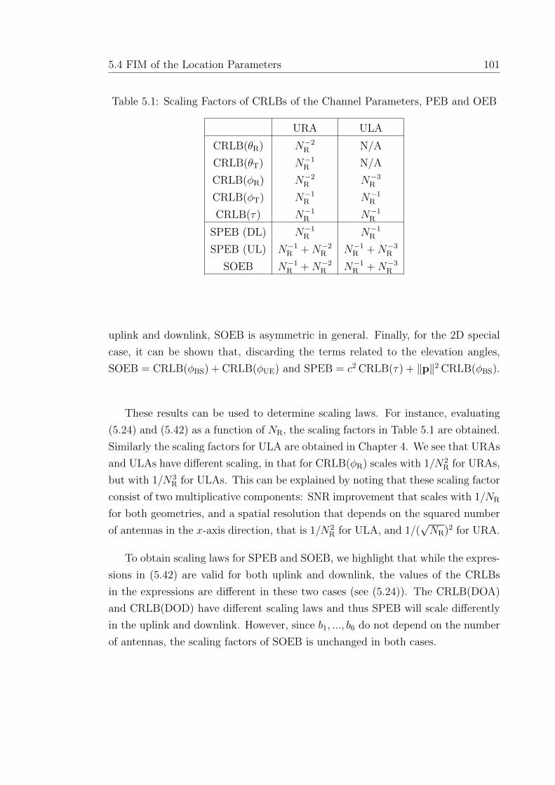
5.4 FIM of the Location Parameters 101
Table 5.1: Scaling Factors of CRLBs of the Channel Parameters, PEB and OEB
URA ULA
CRLB(θR) N−2R N/A
CRLB(θT) N−1R N/A
CRLB(φR) N−2R N−3
R
CRLB(φT) N−1R N−1
R
CRLB(τ) N−1R N−1
R
SPEB (DL) N−1R N−1
R
SPEB (UL) N−1R +N−2
R N−1R +N−3
R
SOEB N−1R +N−2
R N−1R +N−3
R
uplink and downlink, SOEB is asymmetric in general. Finally, for the 2D special
case, it can be shown that, discarding the terms related to the elevation angles,
SOEB = CRLB(φBS) + CRLB(φUE) and SPEB = c2 CRLB(τ) + ‖p‖2 CRLB(φBS).
These results can be used to determine scaling laws. For instance, evaluating
(5.24) and (5.42) as a function of NR, the scaling factors in Table 5.1 are obtained.
Similarly the scaling factors for ULA are obtained in Chapter 4. We see that URAs
and ULAs have different scaling, in that for CRLB(φR) scales with 1/N2R for URAs,
but with 1/N3R for ULAs. This can be explained by noting that these scaling factor
consist of two multiplicative components: SNR improvement that scales with 1/NR
for both geometries, and a spatial resolution that depends on the squared number
of antennas in the x-axis direction, that is 1/N2R for ULA, and 1/(
√NR)2 for URA.
To obtain scaling laws for SPEB and SOEB, we highlight that while the expres-
sions in (5.42) are valid for both uplink and downlink, the values of the CRLBs
in the expressions are different in these two cases (see (5.24)). The CRLB(DOA)
and CRLB(DOD) have different scaling laws and thus SPEB will scale differently
in the uplink and downlink. However, since b1, ..., b6 do not depend on the number
of antennas, the scaling factors of SOEB is unchanged in both cases.

102 Uplink and Downlink 3D Localization Error Bounds in 5G mmWave Systems
Figure 5.4: A cell sectorized into three sectors, each served by 25 beams directedtowards a grid on the ground in the downlink (left) and towards a virtual grid inuplink (right). The grid has the same orientation as the UE.
5.5 Numerical Results and Discussion
5.5.1 Simulation Environment
Although the theoretical results are valid for any arbitrary array geometry, we
focus on URAs, as an example of 3D localization. Particularly, we consider a
scenario where a BS with standard square array is located in the xz-plane centered
at the origin with√NBS ×
√NBS antenna elements and a height of hBS = 10
meters. The UE, operating at f = 38 GHz, is equipped with a square array which
have√NUE×
√NUE antenna elements, and assumed to be tilted by an orientation
angle of 0◦ or 10◦ in both azimuth and elevation. We investigate the performance
over a flat 120◦ sector of a sectorized cell with a radius of 50 meters as shown in
Figure 5.4. The UE is assumed to be located anywhere in this sector, which lies
in the plane z = −hBS = −10 meters. Moreover, we consider the ideal sinc pulse
defined in (4.13) so that W 2eff = W 2/3, where W = 125 MHz, Et/Ts = 0 dBm,
N0 = −170 dBm/Hz, and Ns = 16 pilot symbols. The LOS SNR at any location
in the sector is given by SNR[dB] = 144.24 + 20 log10 |β| + 20 log10 ‖aTF‖, with
95% of the locations having an SNR of at least 30 dB. We utilize the directional
beamforming scheme defined in (5.5). In the downlink case, the directions of the
beams are fixed and chosen such that the beams centers are equispaced on the
ground. On the other hand, in the uplink, the centers of beams are fixed and
equispaced on a virtual sector containing the BS. Initially, when the UE has zero
orientation, i.e, lying in the xz-plane and facing the BS (See Figure 5.1), this
virtual sector lies in the horizontal plane z = 0 meters. The beamforming angles

5.5 Numerical Results and Discussion 103
−40
−200
20
40
0 5 10 15 20 25 30
−15
−10
−5
0
5
x-axis
y-axis
z-a
xis
Figure 5.5: An example on beamforming configuration with 4 beams. The right-most device has orientation angles of 30◦, while the other two have 0◦.
Figure 5.6: A scenario with LOS (black), 2 reflectors (blue) and 2 scatterers (red).
are measured with respect to the UE array plane. Thus, when the orientation of
the UE is non-zero, the virtual plane is rotated by the same orientation angles.
Figure 5.4 depicts the sector layout with NB = 25 for both downlink and uplink.
Figure 5.5 provides an example beamforming configuration, where the BS is located
at (0, 0, 0), with beams pointing downwards. A UE is located at (25, 25,−10)
with zero orientation angles, and another UE is located at (−25, 25,−10) with
orientation angles o = [30◦, 30◦]T. The black rectangles denote the array frame

104 Uplink and Downlink 3D Localization Error Bounds in 5G mmWave Systems
of reference of the device. Note that the first UE has reversed beam direction
compared to BS, while the second UE has beam directions reversed and rotated
by [30◦, 30◦]T , so that the beams direction remains constant with respect to the
frame of reference.
The environment comprises scatterers and reflectors, with scatterers distributed
arbitrarily in the 3D space, and reflectors placed close to the sector edge, as shown
in the example scenario in Figure 5.6. We use 5 reflectors placed at the edge of the
sector, not to obscure the area behind them if placed otherwise. We also use 15
scatterers distributed arbitrarily in the volume formed by the sector as base, and the
BS as height. We only consider the clusters that contribute by a power greater than
10% of the LOS power. As shown in Figure 5.7, it is seen that this configuration
leads to a maximum number of paths M = 6 at any location in the studied sector,
which is similar to the probability mass function in [66]. Accordingly, the complex
channel gain of the mth path is modeled by βm = |βm|ejϑm such that
|βm|2 =λ2
(4π)2
1/d21 LOS
ΓR/(d1,m + d2,m)2 reflector
σ2RCS/(4π(dm,1dm,2)2) scatterer,
(5.43)
where ϑ1 = 2πd1/λ and ϑm = 2π(dm,1 + dm,2)/λ for m > 1, while σ2RCS = 50 m2,
and ΓR = 0.7 are the radar cross section, and the reflection coefficient, respectively.
Although our derivations are valid for any path loss model, we use the model in
(5.43) and the corresponding parameters values to get comparative insights into
the role of reflectors and scatterers on the performance bounds. This may not be
the typical case in reality where scatterers are characterized by the roughness of the
surfaces, which would lead to random path loss, and consequently, random PEB
and OEB. The locations of reflectors are computed using the virtual transmitter
method [134], shown in Figure 5.8
We consider 5 scenarios, for each of which we evaluate the PEB and OEB:
1. LOS : Free space propagation only, without NLOS paths.
2. LOS+R: A LOS path and M − 1 reflected NLOS paths.
3. LOS+S : A LOS path and M − 1 scattered NLOS paths.
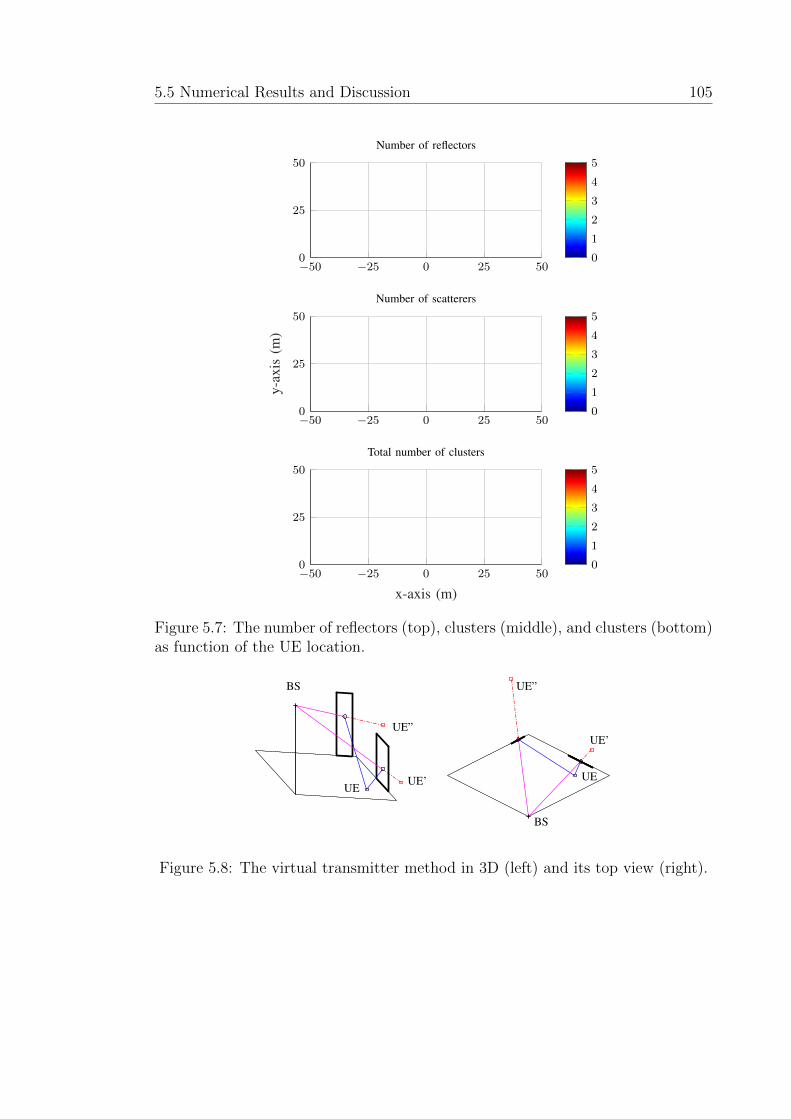
5.5 Numerical Results and Discussion 105
−50 −25 0 25 500
25
50
Number of reflectors
0
1
2
3
4
5
−50 −25 0 25 500
25
50
y-ax
is(m
)
Number of scatterers
0
1
2
3
4
5
−50 −25 0 25 500
25
50
x-axis (m)
Total number of clusters
0
1
2
3
4
5
Figure 5.7: The number of reflectors (top), clusters (middle), and clusters (bottom)as function of the UE location.
BS
UEUE’
UE”
BS
UE
UE’
UE”
Figure 5.8: The virtual transmitter method in 3D (left) and its top view (right).
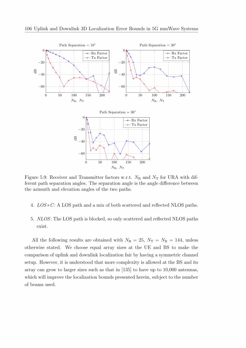
106 Uplink and Downlink 3D Localization Error Bounds in 5G mmWave Systems
0 50 100 150 200
−60
−40
−20
0
NR, NT
dB
Path Separation = 10◦
Rx FactorTx Factor
0 50 100 150 200
−60
−40
−20
0
NR, NT
dB
Path Separation = 20◦
Rx FactorTx Factor
0 50 100 150 200
−60
−40
−20
0
NR, NT
dB
Path Separation = 30◦
Rx FactorTx Factor
Figure 5.9: Receiver and Transmitter factors w.r.t. NR and NT for URA with dif-ferent path separation angles. The separation angle is the angle difference betweenthe azimuth and elevation angles of the two paths.
4. LOS+C : A LOS path and a mix of both scattered and reflected NLOS paths.
5. NLOS : The LOS path is blocked, so only scattered and reflected NLOS paths
exist.
All the following results are obtained with NB = 25, NT = NR = 144, unless
otherwise stated. We choose equal array sizes at the UE and BS to make the
comparison of uplink and downlink localization fair by having a symmetric channel
setup. However, it is understood that more complexity is allowed at the BS and its
array can grow to larger sizes such as that in [135] to have up to 10,000 antennas,
which will improve the localization bounds presented herein, subject to the number
of beams used.

5.5 Numerical Results and Discussion 107
5.5.2 Tx and Rx Factors of the Approximate FIM
We now investigate numerically the trend of the RX and TX factors in (5.12) with
respect to NR and NT and the path separation angles, as shown in Figure 5.9.
Each subfigure is obtained for a different separation angle, that is the azimuth and
elevation angle difference between two paths. It can be seen that with a separation
of 10◦, NR = 100 and NT = 16, the corresponding factor drops below -20 dB
(1% of the maximum). On the other hand, for higher separation angles, the two
factors drop below -20 dB with less number of antennas. Finally, note that the
approximate FIM is obtained by a combined effect of these two factors, plus the
signal factor. Therefore, if NR ≥ 100 or NT ≥ 16, the total FIM will be almost
diagonal.
5.5.3 Downlink PEB and OEB
Figure 5.10 shows the downlink PEB and OEB as a function of the UE location for
the LOS case with the BS located at (0, 0). With NT = NR = 144, and NB = 25,
the maximum PEB in the sector is 40 cm, while the maximum OEB is 1◦ in the
LOS scenario. Note that from (5.42), the PEB increases with ‖p‖. This explains
the dark area around the corners. Moreover, the closer the UE to the BS, i.e., as
θBS → π, singularities appear in the FIM, and the OEB tends to worsen, hence the
dark areas around the BS. Scatterers and reflectors are introduced in the 3D space,
so that a maximum of 5 clusters contribute at any given location. Based on that,
Figure 5.11 shows the PEB and OEB for the LOS+C case. Although incorporating
NLOS clusters in the localization does not lower the maximum bound value, it
improves the bounds at those locations where the clusters’ signal are received. In
the illustrated example, the clusters mainly affect the top and center areas of the
sector. Finally, note the singularity dots in the central area of the PEB and OEB
(LOS+C). These dots occur because at these locations, the scatterer blocks the
LOS, violating the unique parameters assumption, and causing singularities in the
FIM.
To obtain a more concise quantitative assessment of the performance, we collect
all the PEB and OEB values across the space and visualize them in a cumulative
distribution function (CDF). Subsequently, Figure 5.12 shows PEB obtained for

108 Uplink and Downlink 3D Localization Error Bounds in 5G mmWave Systems
−50 −25 0 25 500
25
50
LOS PEB (m)
0
0.1
0.2
0.3
0.4
−50 −25 0 25 500
25
50
x-axis (m)
y-ax
is(m
)
LOS OEB (◦)
0
0.2
0.4
0.6
0.8
1
Figure 5.10: PEB and OEB for downlink LOS. The black dots denote the centersof beams, NB = 25, NR = NT = 144.
all 5 considered scenarios. The PEB obtained from the approximate approach, is
also shown in the figure. We observe the following: overall, scatterers and/or re-
flectors improve the localization performance, compared to the LOS-only scenario,
despite the fact that more parameters need to be estimated. Scatterers are mainly
useful in providing rather low PEB improvement for many locations, while reflec-
tors can provide modest PEB improvement for fewer locations. When scatterers
and reflectors are combined, we see both phenomena. It is also apparent that the
approximate approaches closely follow the exact PEB and OEB and that the ap-
proximation always leads to a slightly lower PEB and OEB, due to the independent
paths assumption, under this approach. Note that at a 90% CDF, the PEB values
for LOS, LOS+R, LOS+S, LOS+C are 0.23 m, 0.21 m, 0.19 m and 0.18 m, re-
spectively. Moreover, note that the NLOS scenario is unreliable, with a PEB of 0.5
m at a 13% CDF, and reaches 90% CDF at a value that is irrelevant in mmWave
localization. OEB curves (not shown) look similar to those in Figure 5.12, with
90% CDF ranging between 0.42◦ and 0.5◦ when a LOS exists. Finally, we obtained

5.5 Numerical Results and Discussion 109
−50 −25 0 25 500
25
50
LOS+C PEB (m)
0
0.1
0.2
0.3
0.4
−50 −25 0 25 500
25
50
x-axis (m)
y-ax
is(m
)
LOS+C OEB (◦)
0
0.2
0.4
0.6
0.8
1
Figure 5.11: PEB and OEB for downlink LOS+C. The black dots denote thecenters of beams, NB = 25, NR = NT = 144.
similar qualitative results with NR = 25, but with PEB and OEB of 45 − 55 cm
and 1.77◦ − 1.84◦, at 90% CDF respectively, when a LOS exists.
5.5.4 The Selection of NB
In this section, we evaluate the impact of the number of beams on downlink lo-
calization. Considering directional beamforming and a given number of transmit
antennas, i.e., a fixed beamwidth, the selection of NB becomes a trade-off between
hardware complexity and the coverage area up to a certain value of NB, where more
beams do not necessarily assist the localization. This relationship is highlighted
in Figure 5.13 for PEB values across the space, at a CDF of 90% (similar results
hold for the OEB, not shown). It can be seen that at a small NB, the bounds
are high, but as NB increases, the bounds start to decrease due better coverage.
However, as NB continues to increase, the bounds reach a floor and adding more
beams only adds more complexity while providing negligible improvement. To see
why, recall that the total transmitted power over the sector is fixed. So, starting

110 Uplink and Downlink 3D Localization Error Bounds in 5G mmWave Systems
0 0.05 0.1 0.15 0.2 0.25 0.30
0.2
0.4
0.6
0.8
1
PEB (m)
CDF
LOSLOS+RLOS+SLOS+CNLOS
Figure 5.12: The CDF of downlink PEB for different scenarios using the exact(solid) and approximate (dashed) FIM approaches.
0 10 20 30 40 50 60 70 80 90 10010−1
100
101
NB
PEB
(m)
NT = 64: LOSNT = 64: LOS+CNT = 144: LOSNT = 144: LOS+C
Figure 5.13: Effect of NB on the exact downlink PEB with NR = 144, NT ∈{64, 144}, for LOS and LOS+C, at CDF = 0.9.
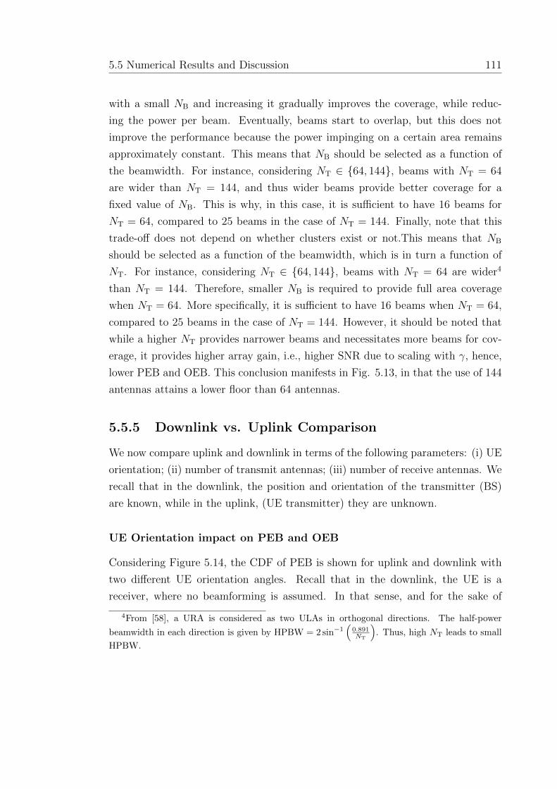
5.5 Numerical Results and Discussion 111
with a small NB and increasing it gradually improves the coverage, while reduc-
ing the power per beam. Eventually, beams start to overlap, but this does not
improve the performance because the power impinging on a certain area remains
approximately constant. This means that NB should be selected as a function of
the beamwidth. For instance, considering NT ∈ {64, 144}, beams with NT = 64
are wider than NT = 144, and thus wider beams provide better coverage for a
fixed value of NB. This is why, in this case, it is sufficient to have 16 beams for
NT = 64, compared to 25 beams in the case of NT = 144. Finally, note that this
trade-off does not depend on whether clusters exist or not.This means that NB
should be selected as a function of the beamwidth, which is in turn a function of
NT. For instance, considering NT ∈ {64, 144}, beams with NT = 64 are wider4
than NT = 144. Therefore, smaller NB is required to provide full area coverage
when NT = 64. More specifically, it is sufficient to have 16 beams when NT = 64,
compared to 25 beams in the case of NT = 144. However, it should be noted that
while a higher NT provides narrower beams and necessitates more beams for cov-
erage, it provides higher array gain, i.e., higher SNR due to scaling with γ, hence,
lower PEB and OEB. This conclusion manifests in Fig. 5.13, in that the use of 144
antennas attains a lower floor than 64 antennas.
5.5.5 Downlink vs. Uplink Comparison
We now compare uplink and downlink in terms of the following parameters: (i) UE
orientation; (ii) number of transmit antennas; (iii) number of receive antennas. We
recall that in the downlink, the position and orientation of the transmitter (BS)
are known, while in the uplink, (UE transmitter) they are unknown.
UE Orientation impact on PEB and OEB
Considering Figure 5.14, the CDF of PEB is shown for uplink and downlink with
two different UE orientation angles. Recall that in the downlink, the UE is a
receiver, where no beamforming is assumed. In that sense, and for the sake of
4From [58], a URA is considered as two ULAs in orthogonal directions. The half-power
beamwidth in each direction is given by HPBW = 2 sin−1(
0.891NT
). Thus, high NT leads to small
HPBW.
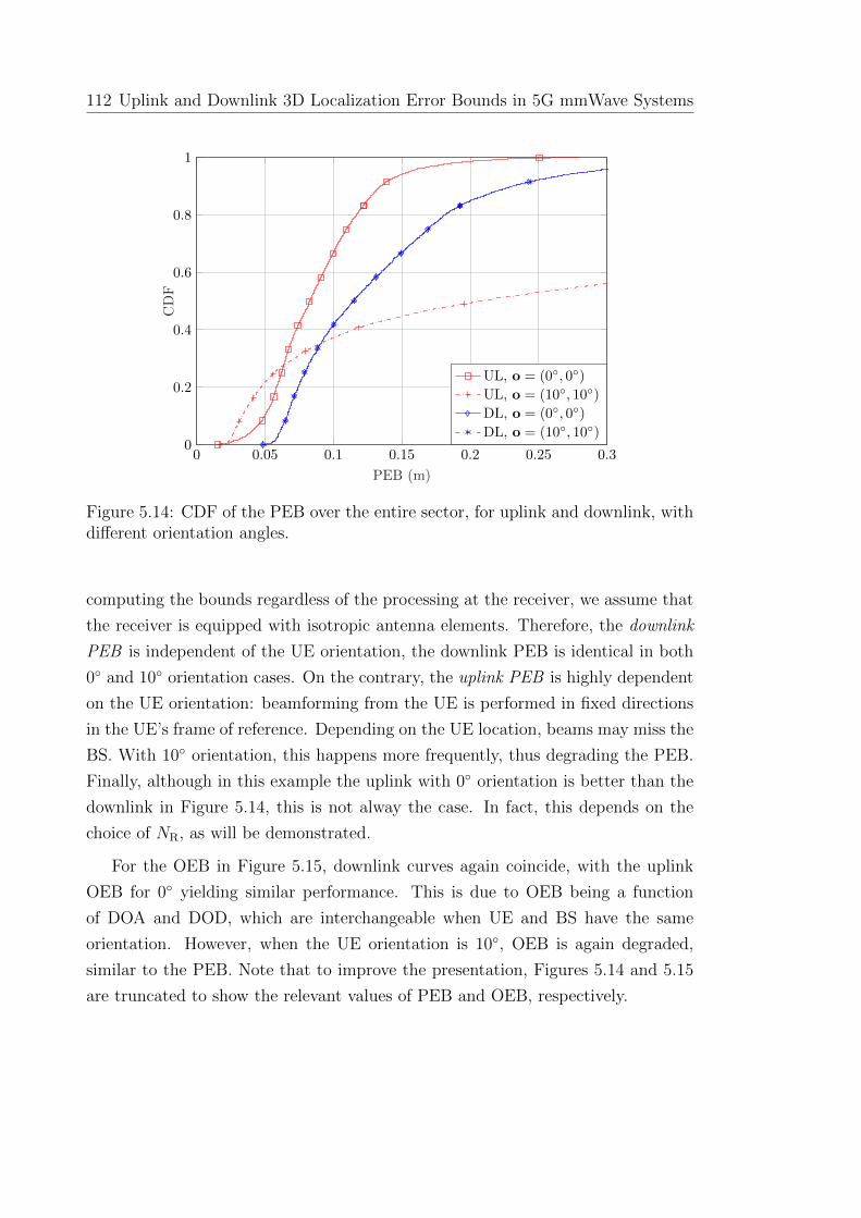
112 Uplink and Downlink 3D Localization Error Bounds in 5G mmWave Systems
0 0.05 0.1 0.15 0.2 0.25 0.30
0.2
0.4
0.6
0.8
1
PEB (m)
CDF
UL, o = (0◦, 0◦)UL, o = (10◦, 10◦)DL, o = (0◦, 0◦)DL, o = (10◦, 10◦)
Figure 5.14: CDF of the PEB over the entire sector, for uplink and downlink, withdifferent orientation angles.
computing the bounds regardless of the processing at the receiver, we assume that
the receiver is equipped with isotropic antenna elements. Therefore, the downlink
PEB is independent of the UE orientation, the downlink PEB is identical in both
0◦ and 10◦ orientation cases. On the contrary, the uplink PEB is highly dependent
on the UE orientation: beamforming from the UE is performed in fixed directions
in the UE’s frame of reference. Depending on the UE location, beams may miss the
BS. With 10◦ orientation, this happens more frequently, thus degrading the PEB.
Finally, although in this example the uplink with 0◦ orientation is better than the
downlink in Figure 5.14, this is not alway the case. In fact, this depends on the
choice of NR, as will be demonstrated.
For the OEB in Figure 5.15, downlink curves again coincide, with the uplink
OEB for 0◦ yielding similar performance. This is due to OEB being a function
of DOA and DOD, which are interchangeable when UE and BS have the same
orientation. However, when the UE orientation is 10◦, OEB is again degraded,
similar to the PEB. Note that to improve the presentation, Figures 5.14 and 5.15
are truncated to show the relevant values of PEB and OEB, respectively.
5.5 Numerical Results and Discussion 113
0 0.1 0.2 0.3 0.4 0.5 0.6 0.7 0.8 0.9 10
0.2
0.4
0.6
0.8
1
OEB (◦)
CDF
UL, o = (0◦, 0◦)UL, o = (10◦, 10◦)DL, o = (0◦, 0◦)DL, o = (10◦, 10◦)
Figure 5.15: CDF of the OEB over the entire sector, for uplink and downlink, withdifferent orientation angles.
Effect of NR and NT
Figure 5.16 shows the scaling effect of the PEB at 90% CDF for LOS, which in line
with Table 5.1, implies that uplink and downlink have different scaling exponents.
This leads the two lines to cross at some value. So, regarding PEB, choosing
NR on either side of this crossing point dictates the outperforming scheme, uplink
or downlink. Specifically, for very large number of receive antennas, uplink PEB
becomes far better than downlink PEB. With reference to Table 5.1 and (??),
downlink PEB ∝ 1√NR
, while uplink PEB ∝√
c1NR
+ c2N2
R, for some constants c1,
and c2 that depend on location, bandwidth, and path gain. For the uplink case,
the first term corresponds to CRLB(TOA), while the second term corresponds
to CRLB(DOA), from Figure 5.16, it can be inferred that CRLB(TOA) is much
smaller than CRLB(DOA) yielding uplink PEB ∝ 1NR
, which decays faster than
PEB ∝ 1√NR
. This also means that the estimation of the UE location is limited by
the estimation of the angles rather than the range.
From Table 5.1, however, the OEB scaling is different than PEB. This is con-
firmed by the results of the OEB at 90% CDF for LOS shown in Figure 5.17. It
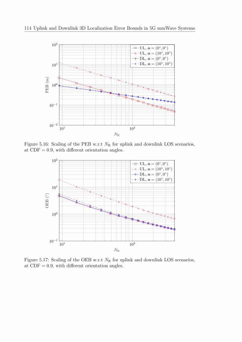
114 Uplink and Downlink 3D Localization Error Bounds in 5G mmWave Systems
101 10210−2
10−1
100
101
102
NR
PEB
(m)
UL, o = (0◦, 0◦)UL, o = (10◦, 10◦)DL, o = (0◦, 0◦)DL, o = (10◦, 10◦)
Figure 5.16: Scaling of the PEB w.r.t NR for uplink and downlink LOS scenarios,at CDF = 0.9, with different orientation angles.
101 10210−1
100
101
102
NR
OEB
(◦)
UL, o = (0◦, 0◦)UL, o = (10◦, 10◦)DL, o = (0◦, 0◦)DL, o = (10◦, 10◦)
Figure 5.17: Scaling of the OEB w.r.t NR for uplink and downlink LOS scenarios,at CDF = 0.9, with different orientation angles.
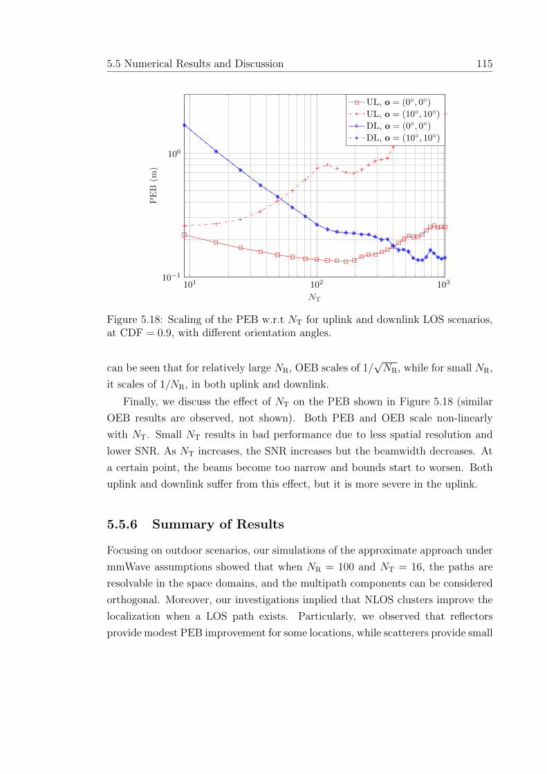
5.5 Numerical Results and Discussion 115
101 102 10310−1
100
NT
PEB
(m)
UL, o = (0◦, 0◦)UL, o = (10◦, 10◦)DL, o = (0◦, 0◦)DL, o = (10◦, 10◦)
Figure 5.18: Scaling of the PEB w.r.t NT for uplink and downlink LOS scenarios,at CDF = 0.9, with different orientation angles.
can be seen that for relatively large NR, OEB scales of 1/√NR, while for small NR,
it scales of 1/NR, in both uplink and downlink.
Finally, we discuss the effect of NT on the PEB shown in Figure 5.18 (similar
OEB results are observed, not shown). Both PEB and OEB scale non-linearly
with NT. Small NT results in bad performance due to less spatial resolution and
lower SNR. As NT increases, the SNR increases but the beamwidth decreases. At
a certain point, the beams become too narrow and bounds start to worsen. Both
uplink and downlink suffer from this effect, but it is more severe in the uplink.
5.5.6 Summary of Results
Focusing on outdoor scenarios, our simulations of the approximate approach under
mmWave assumptions showed that when NR = 100 and NT = 16, the paths are
resolvable in the space domains, and the multipath components can be considered
orthogonal. Moreover, our investigations implied that NLOS clusters improve the
localization when a LOS path exists. Particularly, we observed that reflectors
provide modest PEB improvement for some locations, while scatterers provide small

116 Uplink and Downlink 3D Localization Error Bounds in 5G mmWave Systems
PEB decrease for more locations. Our analysis of the impact of the NB and NT
showed that although smaller NT provide better coverage due to the wider beams,
larger NT provides higher SNR, leading to lower PEB and OEB. We also observed
that PEB and OEB are more sensitive to the orientation angle in the uplink than
in the downlink. Finally, we showed that under mmWave assumptions, PEB < 1
meters and OEB < 1◦ are feasible for BS-UE separation of up to 50 m.
5.6 Conclusions
In this Chapter, we considered mmWave localization performance limits in terms
of PEB and OEB, for uplink and downlink localization with arbitrary array ge-
ometries in multipath environments. We obtained these bounds by transforming
the FIM of the channel parameters that was shown to be composed of three factors
related to the receiver side, the transmitter side, and the transmitted signals. Our
investigations of an approximate approach under mmWave assumptions showed
that if the number of antennas at the receiver is very high, or if the bandwidth is
very large, the paths are resolvable in either the time or space domains, and the
multipath components can be considered orthogonal. Consequently, the total FIM
is the sum of the FIM of individual paths. We also derived closed-form expressions
for single-path PEB and OEB, and showed that OEB is a function of the CRLB
of the DOA and DOD, while PEB is a function of the CRLB of the TOA and the
CRLB of the BS angles (DOD in the downlink, and DOA in the uplink).
Focusing on outdoor scenarios, our simulations show that the NLOS clusters
improve the localization when a LOS path exists. Particularly, we observed that
reflectors provide modest PEB improvement for some locations, while scatterers
provide small PEB decrease for more locations. We analyzed the impact of the
number of beams, and the number of transmit and receive antennas. Although
having many receive antennas is more beneficial in uplink localization than in
downlink localization, the former is generally harder since transmit beamforming
at UE may point towards directions not useful for localization. Finally, we observed
that PEB and OEB are more sensitive to the orientation angle in the uplink than
in the downlink.

5.6 Conclusions 117
Publications Resulted from This Chapter
� Z. Abu-Shaban, X. Zhou, T. Abhayapala, G. Seco-Granados, H. Wymeer-
sch, “Error Bounds for Uplink and Downlink 3D Localization in 5G mmWave
Systems,” Accepted in IEEE Transactions on Wireless Communication, April
2018.
� Z. Abu-Shaban, X. Zhou, T. Abhayapala, G. Seco-Granados, H. Wymeer-
sch “Location and Orientation Estimation Performance with Uplink and
Downlink 5G mmWave Multipath Signals” in the proceedings of IEEE Wire-
less Communications and Networking Conf. (WCNC), Barcelona, Spain,
April 2018.

Chapter 6
Two-Way Localization Bounds for
5G mmWave Systems
Overview: In Chapter 5, we have seen that 5G mmWave localization is promis-
ing with error being in the order centimeters. An assumption usually made in the
investigation of localization methods is that the UE and BS are synchronized. This
was also the case in Chapter 5. However, in reality communications systems are
not finely synchronized to a level useful for localization. Therefore, in this Chapter
we investigate two-way localization protocols that alleviate the need for high-level
of synchronization. Namely, we consider a distributed localization protocol (DLP),
whereby the BS and UE exchange signals in two rounds of transmission and then
localization is achieved using the signal received in the second round. On the other
hand, we consider a centralized localization protocol (CLP), whereby localization is
achieved using the signals received after the two rounds of transmission, where the
first signal is assumed to be fed-back to the first device without error. We derive the
PEB and OEB applying beamforming at both ends, and compare them to the tradi-
tional one-way localization (OWL). Our results show that CLP outperforms DLP
by a significant margin, and that DLP barely outperforms OWL because mmWave
localization is mainly limited by angular rather than temporal estimation. Our sim-
ulations also show that it is more beneficial to have more antennas at the BS than
at the UE.
119

120 Two-Way Localization Bounds for 5G mmWave Systems
6.1 Introduction
Recently, the accuracy of single-anchor localization for 5G mmWave systems has
been studied in several papers in terms of position (PEB) and orientation error
bounds (OEB). In [125], the UE PEB and OEB of 2D localization were inves-
tigated using ULAs in 5G mmWave systems. Moreover, [127] and our work in
Chapter 5 derived, with different approaches, the PEB and OEB for mmWave 3D
localization using arrays with arbitrary geometry. The results in [125, 127, 136]
showed a 5G mmWave localization performance with error in the order of centime-
ters. However, one important, yet usually overlooked, requirement for localization
is the synchronization of BS and UE. For example, [125] and our work in Chapter 5
assume that the BS and UE are perfectly synchronized, while [127] assumes coarse
synchronization, and includes a residual synchronization error in their model.
Inspired by two-way ranging methods [36, 137, 138], where the time-of-flight
is utilized to estimated the range, in this Chapter, we focus on cooperative two-
way localization (TWL). We study the PEB and OEB under line-of-sight (LOS)
communication with two TWL protocols that account for timing bias between the
clocks of the BS and UE. Higher order artifacts such as clock drift and skew are not
addressed herein, but can be estimated using the so-called three-way ranging [36]
or multi-way ranging [139,140]. Under TWL, a device transmits a known signal to
a receiver, which responds by transmitting another known signal. Upon receiving
the latter signal, the first device can estimate the range between the two devices
with reference to its local clock. Since this clock was originally used to transmit
the first signal, it will alleviates the need for fine time synchronization. In the first
protocol, referred to as Distributed Localization Protocol (DLP), a device initiates
the localization process. Then, a second device estimates the TOA with reference
to its local clock and, after a pre-agreed interval, transmits back another signal.
Subsequently, localization is carried out using the signal received back at the first
device. On the contrary, in the second protocol, referred to as Centralized Local-
ization Protocol (CLP), the BS and UE are assumed to be coarsely synchronized,
so that the two transmission rounds take place in non-overlapping time frames.
Under coarse synchronization, the clocks will still have residual bias. Moreover,
the pre-agreed waiting interval is taken with reference to the clock of the first de-
6.2 Channel Model and Beamforming 121
vice, and localization is achieved using the signals received at both devices. In this
context, the signal received at the second device is assumed to be fed-back to the
first device via an error-free link. Note that TWL can be either uplink or downlink,
depending on the device where localization is executed. Finally, the contributions
of this Chapter are summarized as follows
� We investigate the DLP and CLP for LOS 5G mmWave signals, as a means
of alleviating the fine synchronization requirement of 5G localization.
� We derive the FIMs of the position and orientation of the two protocols
using 5G mmWave signals, with the timing bias between the BS and UE as
a nuisance parameter.
� Unlike [125, 127, 136], we consider multi-direction receive beamforming, and
account for the spatially correlated noise resulting from this beamforming.
� Based on the derived FIMs, we evaluate the PEB and OEB numerically for
different protocols, and investigate the impact of the number of antennas at
BS and UE, as well as the bandwidth.
The rest of the Chapter is organized as follows. In Section 6.2, we provide the
system model and highlight the underlying assumptions, while in Section 6.3, we
present the DLP and CLP in detail. In Section 6.4, we derive the PEB and OEB for
the two protocols, first by calculating the channel parameter FIM, then applying
a transformation of variables. In Section 6.5, we provide the numerical results and
the discussion, while in Section 6.6, we draw the conclusions.
6.2 Channel Model and Beamforming
Based on the system geometry detailed in Section 5.2.1, we consider two-way local-
ization protocols in which either BS or UE initiates the protocol. Thus, we denote
the device initiating the protocol by D1 and the responding device by D2.
Notes on notation: In the following, all parameters related to D1 are denoted by
the subscript “1”, while those related to D2 are denoted by the subscript “2”.
Moreover, the superscripts “f” and “b” are used to relate the parameters to the

122 Two-Way Localization Bounds for 5G mmWave Systems
Forward Transmission
Backward Transmission
F1,W1, s1(t),y1(t),n1(t)
θ1, φ1, N1, NB1 ,a1,∆1
No clock bias
Transmit at t = 0
Receive at t = τb
D2D1
F2,W2, s2(t),y2(t),n2(t)
θ2, φ2, N2, NB2 ,a2,∆2
Clock bias: B
Transmit at t = tb
Receive at t = τ f
Figure 6.1: Summary of parameters at D1 and D2. Although D1 and D2 in thefigure are BS and UE, this assignment can be reversed.
forward and backward transmissions, respectively. Finally, unless otherwise stated,
all the provided times are with respect to the clock of D1, which is considered a
global clock. See Fig. 6.1
Forward Channel
The forward signal, transmitted from D1 at time t = 0, and received at D2 at time
t = τ f , undergoes a forward channel given by
Hf(β,ϑ) , Hfs(β,ϑ)δ(t− τ f),∈ CN2×N1 (6.1)
where δ(t) is the Dirac delta function, and Hfs(β,ϑ) is the channel part correspond-
ing the spatial channel parameters, such that
Hfs(β,ϑ) ,
√N1N2βa2(θ2, φ2)aH
1 (θ1, φ1), (6.2)
where β is the complex LOS path gain, N1 and N2 are the number of antennas at
D1 and D2, respectively, while
ϑ , [θ1, φ1, θ2, φ2]T, (6.3)
and (θ2, φ2) and (θ1, φ1) are the forward DOAs and DODs at D2 and D1, respec-
tively. Finally, a2 and a1 are the response vectors at D2 and D1, respectively, given
6.2 Channel Model and Beamforming 123
by
a1(θ1, φ1) ,1√N1
e−j∆T1 k(θ1,φ1), ∈ CN1 (6.4)
a2(θ2, φ2) ,1√N2
e−j∆T2 k(θ2,φ2), ∈ CN2 (6.5)
where k(θ, φ) is the wavenumber vector, ∆1 ∈ C3×N1 is a matrix whose columns
contain the 3D Cartesian coordinates of the array elements of D1 in meters, and
∆2 ∈ C3×N2 is defined similarly for D2. For presentation purposes, we drop the
angle parameters from the notation of a1 and a2.
The signal transmitted from D1 is modeled by√EtF1s1(t), where Et is the
transmitted energy per symbol, and
F1 , [f1,1, f1,2, ...f1,NB1]. (6.6)
is a D1 transmit beamforming matrix, f1,b, 1 ≤ b ≤ NB1 is the bth transmit beam,
and NB1 is the number of transmit beams. The pilot signal s1(t) , [s1,1(t), s1,2(t),
..., s1,NB1(t)]T is written as
s1,b(t) =Ns−1∑
`=0
a(b)1,`p(t− `Ts), 1 ≤ b ≤ NB1 , (6.7)
where a(b)1,` are known unit-energy pilot symbols transmitted over the bth beam from
D1. Similarly, define the receive beamforming matrix at D2 as
W2 , [w2,1,w2,2, ...w2,NB2], (6.8)
where w2,k, 1 ≤ k ≤ NB2 is a D2 receive beam, and NB2 is the number of receive
beams.
Backward Channel
Similarly, the backward channel from D2 to D1 is defined as
Hb(β,ϑ) , Hbs (β,ϑ)δ(t− τb) ∈ CN1×N2 , (6.9)

124 Two-Way Localization Bounds for 5G mmWave Systems
where
Hbs (β,ϑ) ,
√N1N2βa1(θ1, φ1)aH
2 (θ2, φ2), (6.10)
where τb denotes the local TOA at D2, (θ2, φ2) and (θ1, φ1) are the backward DODs
and DOAs at D2 and D1, respectively. We assume that both transmissions occur
within the coherence time, so that the channel gain remains unchanged.
In the backward transmission, D2 transmits via a beamforming matrix, F2
containing NB2 beams, while D1 receives via a beamforming matrix, W1 containing
NB1 beams. Both F2 and W1 are defined similar to W2 and F1, respectively, but
with possibly different beam directions.
Our objective is to derive the performance bounds of estimating p and o, via
TOA, DOA, and DOD, in the presence of the unknown nuisance parameters: timing
offset between the BS and UE clocks, B, and the unknown path gain, β. This will
be done for the DLP and CLP protocols described below.
6.3 Two-Way Localization Protocols
In this section, we define two different two-way localization protocols with the aid
of Fig. 6.2.
6.3.1 General Operation
In our formulation, we assume that D1 has no timing bias, while D2 has a clock
bias with respect to the clock at D1, denoted by B. We also denote the nominal
TOA by τ = ‖p‖/c, where c is the speed of light.
1. Forward Transmission is initiated by D1 at time t = 0, and received at D2
at local time
t = τ f = B + τ. (6.11)
The received signal after beamforming at D2 is given by
y2(t) =√EtW
H2 Hf
s(β,ϑ)F1s1(t− τ f) + n2(t), (6.12)

6.3 Two-Way Localization Protocols 125
D1 D2
t = 0
s1(t)
τ +B
τ −B
τ f = τ +B
y2(t)
tb = τ f + τD
s2(t)τb = 2τ + ef + τD
y1(t)
τD
(a) Distributed Localization Protocol
D1 D2
t = 0
s1(t)τ f = τ +Bτ +B
y2(t)
t = tb
s2(t)τb = τ + tb −B
y1(t)
tb −B
τ
(b) Centralized Localization Protocol
Figure 6.2: The timeline of the studied TWL protocols .
We determine the FIM of[ϑT, βR, βI, τ
f]T
based on y2(t), and denote the
equivalent FIM (EFIM) of τ f by Jτ f .
2. Backward Transmission is initiated by D2 at time t = tb, and received at
D1 at local (which is in the case of D1 is also global) time
t = τb = tb + τ −B. (6.13)
The received signal after beamforming at D1 is
y1(t) =√EtW
H1 Hb
s (β,ϑ)F2s2(t− τb) + n1(t) (6.14)
Based on y1(t), we determine the FIM of[ϑT, βR, βI, τ
b]T
and EFIM of τb,
denoted by Jτb .
126 Two-Way Localization Bounds for 5G mmWave Systems
We introduce the following estimation error notation
ef , τ f − τ f , and eb , τb − τb, such that (6.15)
E{(ef)2} ≥ J−1
τ f, E{
(eb)2} ≥ J−1
τb. (6.16)
Note that, since the received signals are observed at the beamformer output,
n2(t) and n1(t) in (6.12) and (6.14) are zero-mean additive spatially-correlated
Gaussian processes. Therefore, the corresponding auto-covariance matrices are
Rn2 = N0WH2 W2, and Rn1 = N0W
H1 W1. N0 is assumed identical at BS and UE.
The main difference between DLP and CLP is how each protocol coordinates
the response message from D2. In the following, we describe each of these protocols.
6.3.2 Distributed Localization Protocol (DLP)
After a pre-agreed delay τD, measured from the time y2(t) is received, D2 sends
back a signal s2(t) at tb = τ f + τD. See Fig. 6.2(a). Subsequently, D1 receives the
signal y1(t) at
τb = τ f + τD + τ −B = 2τ + ef + τD. (6.17)
Finally, based on y1(t), D1 estimates τb and eventually determines p, and o. Note
that B in the forward and backward transmissions cancel out, and need not be
estimated at D2.
6.3.3 Centralized Localization Protocol (CLP)
We assume that D1 and D2 are coarsely synchronized to avoid overlapping trans-
missions. At this level of synchronization, there is still some residual clock bias,
typically, in the order of hundreds of microseconds. In light of Fig. 6.2.(b), in CLP,
tb is a pre-agreed time with reference to the clock of D2 (tb − B with reference to
the clock of D1), known to both D1 and D2. Upon receiving the signal of D1, D2
sends back a signal s2(t) at t = tb, which is received at D1 at τb given in (6.13).
In parallel to that, D1 also receives y2(t) via an error-free feedback link that can
possibly be established using a microwave channel. Finally, based on y1(t) and the

6.4 Derivation of Two-Way PEB and OEB 127
fed-back y2(t), D1 estimates p, and o.
Under CLP, we determine the FIM of[ϑT, βR, βI, τ, B
]Tbased on both y1(t)
and y2(t). Since the transmissions occur over non-overlapping interval, they provide
independent information. We use this fact to sum up the FIMs of the forward and
backward directions in the following section.
6.4 Derivation of Two-Way PEB and OEB
The PEB and OEB can be computed from the EFIM of position and orientation,
obtained by the transformation of channel parameters; DOA, DOD, and TOA.
Therefore, for both DLP and CLP, we start by computing the FIM of the channel
parameters before deriving the corresponding PEB and OEB using a parameter
transformation procedure similar to that used in Chapter 5.
6.4.1 PEB and OEB for DLP
To compute the PEB and OEB, it is sufficient to obtain the EFIM of position and
orientation, and then use Definition 5.2.
FIM of Channel Parameters
In light of (6.10), (6.14), and (6.17), the vector of the unknowns under DLP is
ϕD ,[ϑT, βR, βI, τ
]T. (6.18)
Consequently, the FIM of ϕD is defined as
JϕD,
[Jb
SS 06
0T6 Jττ
], (6.19)
where,
JbSS =
[Jbϑϑ Jb
ϑβ(Jbϑβ
)TJbβRβR
I2
], (6.20)
128 Two-Way Localization Bounds for 5G mmWave Systems
is the FIM corresponding to the spatial part of JϕD, such that
Jbϑϑ ,
Jbθ1θ1
Jbθ1φ1
Jbθ1θ2
Jbθ1φ2
Jbθ1φ1
Jbφ1φ1
Jbφ1θ2
Jbφ1φ2
Jbθ1θ2
Jbφ1θ2
Jbθ2θ2
Jbθ2φ2
Jbθ1φ2
Jbφ1φ2
Jbθ2φ2
Jbφ2φ2
, (6.21)
and
Jϑβ ,
Jbθ1βR
Jbθ1βI
Jbφ1βR
Jbφ1βI
Jbθ2βR
Jbθ2βI
Jbφ2βR
Jbφ2βI
. (6.22)
Note that the mutual information between the temporal and spatial parts in (6.19)
is zero based on realistic mmWave assumptions of large number of antennas at the
transmitter and receiver, large bandwidth and spatially sparse channel. Moreover,
note that, in (6.20), we used the fact that JbβRβR
= JbβIβI
.
While we can determine Jτ f based on y2(t), the FIM of[ϑT, βR, βI, τ
b]T
is based
on y1(t). To obtain the FIM of ϕD that includes τ rather than τb, we apply the
fact that the delays are not dependent on any of the other parameters proven in
Chapter 5. Towards that, recall that τb = 2τ + ef + eb + τD, and define
τ ′ ,τb − τD
2= τ +
ef + eb
2. (6.23)
Consequently, using (6.16) yields
E{
(τ ′ − τ)2}≥ 1
4
(J−1τ f
+ J−1τb
), (6.24)
that is,
Jττ = 4(J−1τ f
+ J−1τb
)−1. (6.25)
The value of Jττ as well as the entries of (6.20) are listed in (G.6) and (G.7), derived
in Appendix G.

6.4 Derivation of Two-Way PEB and OEB 129
FIM of Location Parameters
To obtain the FIM of the location parameters (position and orientation), we need
the EFIM of ϑ and τ . Since the temporal and spatial parts in (6.19) are indepen-
dent, the EFIM of DOD and DOA is obtained from (6.20) by Schur’s complement
Je,bϑϑ = Jb
ϑϑ −1
JbβRβR
Jbϑβ
(Jbϑβ
)T. (6.26)
Consequently, the EFIM of ϑ and τ is given by
Je,bϑτ =
[Je,bϑϑ 04
0T4 Jττ
]. (6.27)
Applying a parameter transformation to (6.27), we obtain the EFIM of o and p
Je,bo,p = ΥbJe,b
ϑτ
(Υb)T, (6.28)
where
Υb ,
[∂θ1∂o
∂φ1∂o
∂θ2∂o
∂φ2∂o
∂τ∂o
∂θ1∂p
∂φ1∂p
∂θ2∂p
∂φ2∂p
∂τ∂p
]=[
Υbs Υτ
]. (6.29)
Note that while
Υτ =[0T
2pT
c‖p‖
]T
, (6.30)
for both the uplink and downlink, Υbs is defined differently. From Chapter 5
Υbs |UL =
0 0 −p′ya′ −p′xp
′z
a′2
0 0 p′x sin θ0a′
−p′2x cos θ0+gp′ya′2
pθ‖p‖a
[−py ,px,0]T
a2
r3+p′z‖p‖p
a′(r2rT1 −r1rT2 )p
a′2
, (6.31)
Υbs |DL =
−p′ya′ −p′xp
′z
a′2 0 0p′x sin θ0
a′−p′2x cos θ0+gp′y
a′2 0 0
r3+p′z‖p‖p
a′(r2rT1 −r1rT2 )p
a′2pθ‖p‖a
[−py ,px,0]T
a2
, (6.32)

130 Two-Way Localization Bounds for 5G mmWave Systems
where g , py cosφ0 − px sinφ0, pθ , [pxpz, pypz,−a2]T, a ,√p2x + p2
y, a′ ,√
p′2x + p′2y , [p′x, p′y, p′z]
T , Rp, and R , [r1, r2, r3] is the rotation matrix as defined
in (5.35).
Subsequently, for DLP, we can isolate the spatial and temporal parts and write,
Je,bo,p = Υb
s Je,bϑϑ
(Υb
s
)T
︸ ︷︷ ︸Spatial Part
+ JττΥτΥTτ︸ ︷︷ ︸
Temporal Part
. (6.33)
6.4.2 PEB and OEB for CLP
FIM of Channel Parameters
Unlike DLP, in CLP we have to retrieve B, as can be inferred from (6.11) and
(6.13). Therefore, we define the vector of unknown parameters as
ϕC ,[ϑT, βR, βI, τ, B
]T. (6.34)
Since D2 transmission time is independent of the TOA of y2(t), and the trans-
mission in the two ways occurs in a non-overlapping time slots, the forward and
backward transmissions can be considered independent, and we can write
JϕC= Jf
ϕC+ Jb
ϕC,
=
[Jf
SS 06×2
02×6 JfTT
]+
[Jb
SS 06×2
02×6 JbTT
]. (6.35)
where the superscripts “f”, “b” indicate that the FIM is of the channel parameters
from forward and backward transmission, respectively. Note that while JbSS in (6.20)
can be directly obtained from (G.6), JfSS is obtained by swapping the subscripts
“1” and “2” of the right-hand side of (G.6) in Appendix G.
Moreover, JfTT and Jb
TT ∈ R2×2 are the FIMs of the temporal parameters, τ
and B, in the forward and backward transmission, respectively, such that
JfTT ,
[J fττ J f
τB
J fτB J f
BB
](6.36)

6.4 Derivation of Two-Way PEB and OEB 131
and JbTT is defined similarly with matching superscripts.
To obtain JfTT and Jb
TT, we use transformation of variables. From (6.11)
JfTT =
[∂τ f
∂τ∂τ f
∂B
]Jτ f[∂τ f
∂τ∂τ f
∂B
]= Jτ f
[1 1
1 1
]. (6.37)
Similarly, from (6.13)
JbTT =
[∂τb
∂τ∂τb
∂B
]Jτb[∂τb
∂τ∂τb
∂B
]= Jτb
[1 −1
−1 1
]. (6.38)
Note that although both JfTT and Jb
TT are rank-deficient1, their sum is full-rank,
and is given by
JfTT + Jb
TT =
[Jτb + Jτ f Jτ f − JτbJτ f − Jτb Jτb + Jτ f
]. (6.39)
Consequently, the EFIM of τ is obtained from (6.39) by Schur’s complement as
Jeττ = Jτb + Jτ f −
(Jτb − Jτ f )2
Jτb + Jτ f,
=(Jτb + Jτ f )
2 − (Jτb − Jτ f )2
Jτb + Jτ f,
=4JτbJτ f
Jτb + Jτ f,
= 4(J−1τ f
+ J−1τb
)−1(6.40)
which is equivalent to Jττ of DLP given in (6.25).
FIM of Location Parameters
Under CLP, we transform the FIM of the channel parameters vector ϕC into a FIM
of the location parameters vector
ϕL , [oT,pT, βR, βI , B]T, (6.41)
1Hence, τ and B cannot be estimated using only one transmission.

132 Two-Way Localization Bounds for 5G mmWave Systems
as follows
JϕL= ΥbJϕC
(Υb)T
= Υb(JfϕC
+ JbϕC
) (Υb)T,
= ΥbJfϕC
(Υb)T
︸ ︷︷ ︸,Jf
ϕL
+ ΥbJbϕC
(Υb)T
︸ ︷︷ ︸,Jb
ϕL
, (6.42)
such that
Υb =∂ϕT
C
∂ϕL
,
Υbs 05×2 Υτ 05
02×4 I2 02 02
0T4 0T
2 0 1
(6.43)
where Υτ is the transformation vector from τ to o and p defined in (6.30) and Υbs
is the transformation matrix from DOD and DOA to o and p, defined in (6.31)
and (6.32) for the uplink and downlink. Moreover, from (6.20) and (6.35), we write
JbϕC
=
Jbϑϑ Jb
ϑβ(Jbϑβ
)TJbββ
06×2
06×2 JbTT
. (6.44)
Note that JfϕC
is defined similarly with matching superscripts.
Substituting Υb, JfϕC
and JbϕC
into (6.42), it can be shown that JϕLis given by
JϕL=
Jo,p Υbs
(Jfϑβ + Jb
ϑβ
)(Jτ f − Jτb)Υτ(
Jfϑβ + Jb
ϑβ
) (Υb
s
)TJfββ + Jb
ββ 02
(Jτ f − Jτb)ΥTτ 0T
2 Jτb + Jτ f
, (6.45)
where Jo,p = Υbs
(Jfϑϑ + Jb
ϑϑ
) (Υb
s
)T+ (Jτb + Jτ f )ΥτΥ
Tτ .
Finally, taking the Schur’s Complement with respect to Jo,p, and using (6.26),
and (6.40), it can be shown that the EFIM of the position and orientation is
J(e)o,p =Υb
s
(Jfϑϑ + Jb
ϑϑ
)(Υb
s
)T+
(Jτb + Jτ f −
(Jτb − Jτ f )2
Jτb + Jτ f
)Υτ (Υτ )T
−Υbs
(Jfϑβ + Jb
ϑβ
)(Jfββ + Jb
ββ
)−1 (Jfϑβ + Jb
ϑβ
)(Υb
s
)T.
6.4 Derivation of Two-Way PEB and OEB 133
= Υbs Je,fϑϑ
(Υb
s
)T
︸ ︷︷ ︸Forward Spatial Part
+ Υbs Je,bϑϑ
(Υb
s
)T
︸ ︷︷ ︸Backward Spatial Part
+ JeττΥτΥ
Tτ︸ ︷︷ ︸
Temporal Part
+JbβRβR
J fβRβR
J fβRβR
+ JbβRβR
JfbJTfb
︸ ︷︷ ︸Channel Redundant Information
,
(6.46)
where Jfb = Υbs
(Jfϑβ
J fβRβR
− Jbϑβ
JbβRβR
). In the following, we obtain some insights from this
equation.
6.4.3 Comparison of DLP, CLP and OWL
It can be seen that (6.46) comprises four terms: two spatial information terms
related to both the forward and backward transmissions, one term related to the
temporal information, and another term, carrying mutual information relating the
path gain with the DOA and DOD. Note that although we assume a single β in
both transmissions, it is estimated using two different observations, y1(t) and y2(t).
This provides more spatial information useful in localization, since the path gain,
DOA and DOD are not mutually independent (See (6.20)). Moreover, this mutual
information is non-zero due to having different beamformers at both ends, henceJfϑβ
J fβRβR
6= Jbϑβ
JbβRβR
.
Comparing DLP to CLP, we note that (6.33) contains only one spatial informa-
tion term, related to the backward transmission, and another temporal information
term. These two terms are equal to their counterparts in (6.46). Since CLP has
two more terms, it provides more information on the position and orientation, and
consequently lower PEB and OEB. Thus, CLP will always outperform DLP.
We now compare DLP to the one-way localization (OWL) presented in Chapter
5. Recall that for OWL, Je,bo,p has the same expression as (6.33), but with
Jττ = Jτb . (6.47)
Based on that, we provide the following proposition.
Proposition 6.1 DLP outperforms OWL if,
Jτ f >1
3Jτb .

134 Two-Way Localization Bounds for 5G mmWave Systems
Proof
Comparing DLP with OWL, it can be seen that they have equal spatial, but dif-
ferent temporal information. Therefore, comparing (6.25) with (6.47), for DLP to
outperform OWL, we should have
Jτb < 4(J−1τ f
+ J−1τb
)−1= Jτb
4Jτ f
Jτ f + Jτb,
which leads to Jτ f >13Jτb .
This means that, when the bandwidth is equal in both directions, the forward link
should have at least one third the SNR of the backward link for DLP to outperform
OWL. From (G.7), it can be seen that this mainly depends on the beamforming
at the transmitter and receiver. However, under the general case of non-identical
bandwidth allocation, (G.7) can be used to determine the values of bandwidth and
SNR that satisfy the condition in Proposition 6.1.
6.5 Simulation Results and Discussion
6.5.1 Simulation Environment
System Layout and Channel
In our numerical simulations, we investigate and compare the DLP and CLP. Since
both protocols involve forward and backward transmission, we selected equal num-
ber of antennas at both the BS and the UE to make the comparison of these pro-
tocols fair. Towards that, we consider a BS and a UE both with 12 × 12 uniform
rectangular antenna array (URA) communicating via a LOS. Moreover, we assume
that the BS array is located in the xz-plane centered about the origin [0, 0, 0]T, thus
has orientation angles of [0◦, 0◦]T. On the other hand, the UE moves freely within a
diamond-shape 120◦ defined by the vertices {(0, 0,−10), (25√
3, 25,−10), (0, 50,−10),
(−25√
3, 25,−10)}. That is, the BS height is 10 meters. We focus on two cases
of orientation angles with respect to the z-axis and x-axis: o = [θ0, φ0] = [0◦, 0◦]T
and o = [30◦, 30◦]T as specified in the sequel. Finally, at a distance d1, the channel
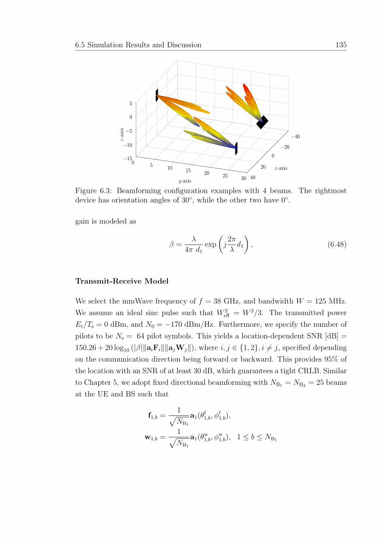
6.5 Simulation Results and Discussion 135
−40
−20
0
20
40
0 5 10 15 20 25 30
−15
−10
−5
0
5
x-axis
y-axis
z-a
xis
Figure 6.3: Beamforming configuration examples with 4 beams. The rightmostdevice has orientation angles of 30◦, while the other two have 0◦.
gain is modeled as
β =λ
4π d1
exp
(j
2π
λd1
), (6.48)
Transmit-Receive Model
We select the mmWave frequency of f = 38 GHz, and bandwidth W = 125 MHz.
We assume an ideal sinc pulse such that W 2eff = W 2/3. The transmitted power
Et/Ts = 0 dBm, and N0 = −170 dBm/Hz. Furthermore, we specify the number of
pilots to be Ns = 64 pilot symbols. This yields a location-dependent SNR [dB] =
150.26 + 20 log10 (|β|‖aiFi‖‖ajWj‖), where i, j ∈ {1, 2}, i 6= j, specified depending
on the communication direction being forward or backward. This provides 95% of
the location with an SNR of at least 30 dB, which guarantees a tight CRLB. Similar
to Chapter 5, we adopt fixed directional beamforming with NB1 = NB2 = 25 beams
at the UE and BS such that
f1,b =1√NB1
a1(θf1,b, φ
f1,b),
w1,b =1√NB1
a1(θw1,b, φ
w1,b), 1 ≤ b ≤ NB1

136 Two-Way Localization Bounds for 5G mmWave Systems
are D1 transmit and receive beams pointing towards (θf1,b, φ
f1,b) and (θw
1,b, φw1,b), re-
spectively. The transmit and receive beamforming at D2 can be similarly defined
with subscript “2”. The directions of the beams at the BS are chosen to be equi-
spaced on the sector. On the UE, these directions are reversed to point upwards,
and rotated with respect to the UE frame of reference by the same orientation an-
gles specified in the studied experiment. This setting provides 90% of the locations
with an SNR of at least 17 dB. Fig. 6.3 provides three examples on beamform-
ing configuration: a BS at (0, 0, 0), with beams pointing downwards, a UE at
(25, 25,−10) with zero orientation angles, and another UE at (−25, 25,−10) with
o = [30◦, 30◦]T. The black rectangles denote the array frame of reference of the
device. Note that the first UE has reversed beam direction compared to BS, while
the second UE has beam directions reversed and rotated by [30◦, 30◦]T , so that the
beams direction remains constant with respect to the UE local frame of reference.
Scenarios Studied
We study the PEB and OEB under DLP and CLP and compare these bounds to
those obtained for OWL in Chapter 5. Each of these three protocols is studied
when localization is performed in the uplink (at BS) and in the downlink (at UE).
6.5.2 PEB and OEB with 0◦ UE Orientation
The PEB with zero orientation angles is provided in Fig. 6.4 for all the considered
protocols. First of all, to have a fair comparison, we compare the three solid curves
corresponding to uplink localization, and then compare those related to downlink
localization (dash-dot lines). It can be seen that DLP provides a negligible improve-
ment over OWL. Despite that, DLP is still a better approach since it alleviates the
need of high-accuracy synchronization, with the cost of UE-BS coordination. As
discussed in Section 6.4.3, DLP and OWL have the same spatial component, but
DLP has higher temporal information content. However, Fig. 6.4 shows almost
identical results for both protocols, which means that the additional temporal in-
formation in DLP is of little importance, and thus the localization performance
is limited by the angles estimation rather than the time delay. To understand
this phenomenon more, we study the impact of the bandwidth on the performance

6.5 Simulation Results and Discussion 137
0 0.02 0.04 0.06 0.08 0.1 0.12 0.14 0.16 0.18 0.20
0.2
0.4
0.6
0.8
1
PEB (m)
CD
F
CPL: BSDPL: BSOWL: BSCPL: UEDPL: UEOWL: UE
Figure 6.4: CDF of PEB with UE orientation angles of 0◦, and NUE = NBS = 144,NB = 25.
0 0.05 0.1 0.15 0.2 0.25 0.3 0.35 0.4 0.45 0.50
0.2
0.4
0.6
0.8
1
OEB (◦)
CD
F
CPL: BSDPL: BSOWL: BSCPL: UEDPL: UEOWL: UE
Figure 6.5: CDF of OEB with UE orientation angles of 0◦, and NUE = NBS = 144,NB = 25.
later in Section 6.5.4. On the other hand, as expected, CLP represents the best
approach among the three studied, since it attains more useful information. How-
ever, this comes with the cost of a more complex implementation due to the need
for a feedback channel.
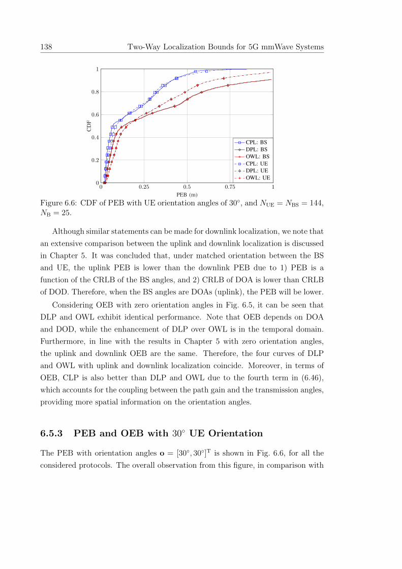
138 Two-Way Localization Bounds for 5G mmWave Systems
0 0.25 0.5 0.75 10
0.2
0.4
0.6
0.8
1
PEB (m)
CD
F
CPL: BSDPL: BSOWL: BSCPL: UEDPL: UEOWL: UE
Figure 6.6: CDF of PEB with UE orientation angles of 30◦, and NUE = NBS = 144,NB = 25.
Although similar statements can be made for downlink localization, we note that
an extensive comparison between the uplink and downlink localization is discussed
in Chapter 5. It was concluded that, under matched orientation between the BS
and UE, the uplink PEB is lower than the downlink PEB due to 1) PEB is a
function of the CRLB of the BS angles, and 2) CRLB of DOA is lower than CRLB
of DOD. Therefore, when the BS angles are DOAs (uplink), the PEB will be lower.
Considering OEB with zero orientation angles in Fig. 6.5, it can be seen that
DLP and OWL exhibit identical performance. Note that OEB depends on DOA
and DOD, while the enhancement of DLP over OWL is in the temporal domain.
Furthermore, in line with the results in Chapter 5 with zero orientation angles,
the uplink and downlink OEB are the same. Therefore, the four curves of DLP
and OWL with uplink and downlink localization coincide. Moreover, in terms of
OEB, CLP is also better than DLP and OWL due to the fourth term in (6.46),
which accounts for the coupling between the path gain and the transmission angles,
providing more spatial information on the orientation angles.
6.5.3 PEB and OEB with 30◦ UE Orientation
The PEB with orientation angles o = [30◦, 30◦]T is shown in Fig. 6.6, for all the
considered protocols. The overall observation from this figure, in comparison with

6.5 Simulation Results and Discussion 139
0 2 4 6 8 10 120
0.2
0.4
0.6
0.8
1
OEB (◦)
CD
F
CPL: BSDPL: BSOWL: BSCPL: UEDPL: UEOWL: UE
Figure 6.7: CDF of OEB with UE orientation angles of 30◦, and NUE = NBS = 144,NB = 25.
Fig. 6.4, is that the performance worsens due to the beams being steered away, when
the orientation angles are non-zero. This can result in a loss of beamforming gain
that depends non-linearly on the UE location, and orientation angles. However,
CLP performance is still superior to DLP and OWL. In this example, performance
loss of 42 cm, 54 cm, and 80 cm were observed at a PEB CDF of 90%, under
CLP, uplink DLP, and downlink DLP, respectively. On the other hand, comparing
Fig. 6.7 with Fig. 6.5, it can be seen that, at a CDF of 90%, there is a OEB
performance loss of 6.8◦, 8.8◦, and 11.5◦ under CLP, uplink DLP, and downlink
DLP, respectively. Considering the PEB and OEB loss, it can be concluded that,
among the studied approaches, CLP is the approach that is most robust to UE
mis-orientation. Finally, we note that in comparison with the case of matched
orientation, under 30◦ mis-orientation, the system can still provide sub-meter PEB,
while providing significantly higher OEB. This means that orientation estimation
is more challenging than position estimation.
6.5.4 Impact of the System Bandwidth on PEB
In Section 6.5.3, we concluded that the system is limited by the estimation of the
angles rather than the time delay. To investigate that further, we now look closer
into the impact of the bandwidth. The results shown in Fig. 6.8 indicate that as

140 Two-Way Localization Bounds for 5G mmWave Systems
10 20 30 40 50 100 150 200
10−1
100
W (MHz)
PEB
(m)
CPL:BSDPL: BSOWL: BSCPL:UEDPL: UEOWL: UE
o = (0◦, 0◦)
o = (30◦, 30◦)
Figure 6.8: PEB at 0.9 CDF with respect to the bandwidth W .
the bandwidth increases the PEB decreases, until it reaches a floor at around 100
MHz when o = [0◦, 0◦]T, and 60 MHz when o = [30◦, 30◦]T. Based on these results,
we make the following observations:
1. At higher bandwidths that are more relevant in mmWave, the temporal infor-
mation is very high compared to the spatial information, and the performance
becomes fixed with W , i.e., the systems is spatially-limited.
2. under mis-orientation, the accuracy of spatial information degrades, and the
system becomes spatially-limited. Hence, the improved temporal informa-
tion does not provide any benefit to the performance achieved at lower band-
widths.
3. On the contrary, for lower bandwidths, the amount of temporal information
decreases and becomes comparable to the spatial information. Therefore,
the weight of the temporal information in the forward transmission becomes
more significant, and the difference between OWL and DLP becomes more
pronounced.
6.5.5 Impact of NBS and NUE on PEB
We now study the effect of the number of antennas at BS and UE on the PEB
under CLP and DLP. Since this number can be N1 or N2 depending on the device

6.5 Simulation Results and Discussion 141
0 100 200 300 400 500 60010−2
10−1
100
101
NUE
PEB
(m)
CPL:BSDPL: BSCPL:UEDPL: UE
o = (0◦, 0◦)
o = (30◦, 30◦)
Figure 6.9: PEB at 0.9 CDF as a function of the UE number of antennas, withNB = 25, with orientation angles 0◦ and 30◦, and NBS = 144.
0 100 200 300 400 500 60010−2
10−1
100
101
NBS
PEB
(m)
CPL:BSDPL: BSCPL:UEDPL: UE
o = (0◦, 0◦)
o = (30◦, 30◦)
Figure 6.10: PEB at 0.9 CDF as a function of the BS number of antennas, withNB = 25, with orientation angles 0◦ and 30◦, and NUE = 144.
role, we use NBS and NUE to unify the notation of the number of antennas at BS
and UE, respectively.
Fig. 6.9 illustrates the effect of NUE on PEB with NB = 25 and NBS = 144.
It can be seen that a higher NUE generally results in a worse performance. This

142 Two-Way Localization Bounds for 5G mmWave Systems
is because with higher NUE, the UE beams become narrower, which requires more
beams to cover the area. Note that with UE mis-orientation, the rate of perfor-
mance deterioration is higher. It is interesting to see that this rate is almost the
same for the three protocols, which means that the performance loss is mainly due
to SNR loss.
On the other hand, the impact of NBS is shown in Fig. 6.10 with NB = 25
and NUE = 144. It can be seen that a higher NBS will slightly improve the PEB
in general. Similar to the case in Fig. 6.9, it is understood that the PEB will
generally increase when NBS increases, albeit, at NBS values well beyond those
displayed in Fig. 6.10, and with a lesser magnitude than higher NUE. Therefore,
adding more antennas at the BS will not reduce the localization performance, as
the UE antennas potentially would, at least within the studied range of array size.
Finally, notice that both Figs. 6.9 and 6.10 exhibit some non-monotonic trend.
This is due to the nature of directional beamforming, whereby the beamforming
gain depends on the user location, number of antennas, and beams directions as
detailed in Chapter 4.
6.6 Conclusions
Many publications on localization assume that the BS and UE are tightly syn-
chronized. However, usually communication systems are not synchronized to a
high-level useful for localization. Focusing on this issue, in this Chapter, we con-
sidered two protocols of two-way localization referred to Distributed Localization
Protocol (DLP) and Centralized Localization Protocol (CLP). We investigated the
PEB and OEB under these two protocols, where we showed mathematically that
CLP outperforms DLP with a significant margin. However, this comes with the
cost of requiring feedback channel, unlike DLP where no synchronization or feed-
back are required, although it may need dedicated hardware to trigger the response.
In our derivations, we considered beamforming at the transmitter and the receiver,
and accounted for the spatially-correlated receive noise. Comparing DLP to the
traditional one-way localization, the enhancement observed through numerical sim-
ulations was limited. That is, the localization was angle-limited rather than delay-
limited. Our numerical results also showed that it is more beneficial to have more

6.6 Conclusions 143
antennas at the BS than at the UE. Future work based on this Chapter includes
considering adaptive beamforming, whereby the beams directions are modified in
the second round of transmission. Moreover, multipath propagation would be a rel-
evant extension, since scatterers may differ in the uplink and downlink, depending
on the beam directions.
Publications Resulted from This Chapter
� Z. Abu-Shaban, H. Wymeersch, T. Abhayapala, G. Seco-Granados, “Single-
Anchor Two-Way Localization Bounds for 5G mmWave Systems: Two Pro-
tocols,” to be submitted to IEEE Transactions on Wireless Communication,
May 2018.
� Z. Abu-Shaban, H. Wymeersch, T. Abhayapala, G. Seco-Granados, “Single-
Anchor Two-Way Localization Bounds for 5G mmWave Systems,” to be sub-
mitted to 2018 IEEE Global Communications Conf. (GLOBECOM Work-
shops), Abu Dhabi, UAE, Dec 2018.


Chapter 7
Conclusions and Future Research
This thesis provided applied and fundamental research results on active areas of
mobile localization, with more focus on 5G mmWave localization performance. In
this chapter, we draw conclusions with respect to the questions posed in this thesis
(Section 1.5) and suggest possible future research directions
7.1 Conclusions
� The problem of multi-anchor localization under mixed LOS and NLOS condi-
tions is addressed in Chapter 3. A key advantage in our work is that it solves
the NLOS UE localization in a closed-form, in contrast to most of works
that are either search-based or iterative. We used a distance-dependent bias
model to derive an unbiased range estimator as a first step. Subsequently,
we used trilateration to find an estimate of the UE position. We then per-
formed error analysis and evaluated numerically the CRLB as a benchmark.
Our approach was to identify the NLOS links and then use a statistical sig-
nal model to account for the positive range bias. Our proposed localization
techniques showed performance close to the CRLB. With a cell radius of 500
m, our method is accurate with an average position error ranging between
12–21 meters depending on the environment. Finally, we note that, although
the proposed method performs closely with the CRLB, the average error ob-
tained is in the order of several meters, which implies that location-aware
145
146 Conclusions and Future Research
communications have limited applications in conventional cellular network.
� Focusing on 2D scenarios of 5G mmWave, the initial access problem was
addressed in Chapter 4. We investigated two beamforming schemes (RPBF
and DBF) and compared their capabilities in terms of the channel parameters’
CRLBs. Our analysis and simulation results showed that in the absence of
any prior location knowledge, application of RPBF is more appropriate in
the considered scenario because it attains a lower CRLBs with fewer beams
compared to DBF. We also observed that in DBF, the CRLBs tend to increase
with NT, while under RPBF, they stay constant. An exception to this is the
CRLB of DOD, which decreases with NT, with varying degrees in RPBF and
DBF. On the other hand, we observed that increasing NR always reduced the
CRLB of all parameters in both schemes. We used CRLB to compare these
two schemes. However, the values of these CRLB are of little importance until
location information is inferred from them, which is the topic of Chapter 5.
� Contributing to the emerging 5G mmWave networks, and focusing on the
localization part of the system beyond the initial access phase, Chapter 5
investigate the position and device orientation estimation error bounds. Both
uplink and downlink localization were considered. Our key findings indicate
that the uplink and downlink behave differently in two distinct ways. First
of all, the error bounds have different scaling factors with respect to the
number of antennas in the uplink and downlink. Secondly, uplink localization
is sensitive to the orientation angle of the UE, whereas downlink is not.
Moreover, in the considered outdoor scenarios, the NLOS paths generally
improve localization when a LOS path exists. We observed that reflectors
provide modest PEB improvement for some locations, while scatterers provide
small PEB decrease for more locations.
� Although having many receive antennas is more beneficial in uplink local-
ization than in downlink localization, the former is generally harder since
transmit beamforming at UE may point towards directions not useful for lo-
calization. We analyzed the impact of the NB, and noticed a saturation effect
appears after some value, after which adding more beams does not enhance

7.2 Future Research Directions 147
the performance. We also studied the impact of NT and NR on PEB and
OEB, and concluded that increasing NR always improves the performance
with the cost of increased hardware and computation complexities. Finally,
our numerical results showed that mmWave systems are capable of localizing
a UE with sub-meter position error, and sub-degree orientation error.
� In Chapter 7 we addressed the synchronization issue of 5G mmWave systems
by studying two-way localization protocols: DLP and CLP. Our studies show
that mmWave localization is mainly limited by angular rather than temporal
estimation. Thus, estimating the DOA and DOD is much harder than TOA,
as far as localization is concerned. We investigated the PEB and OEB under
these two protocols, where we showed mathematically that CLP outperforms
DLP with a significant margin. However, this comes with the cost of requiring
a coarse synchronization, unlike DLP where no synchronization is required.
Our simulations also showed that it is more beneficial to have more antennas
at the BS than at the UE. This is consistent with the results obtained in
Chapter 5, although we did not consider receive beamforming in that Chapter.
The main outcome of this thesis is a fundamental understanding of how 5G
mmWave technology can be an enabler for extremely accurate localization. Through
theoretical performance bounds, we have developed insights as to why and when
5G localization is feasible, how 5G localization systems should be designed, and
how 5G localization and 5G communication can support each other. This thesis
highlights that 5G localization with mmWave technology will play a central role
in communication network optimization and unlock opportunities that were not
available in conventional networks.
7.2 Future Research Directions
Localization in 5G mmWave networks is still in its infancy. This thesis contributed
significantly to the understanding of the factors interplay and the expected er-
ror performance. Our findings in this thesis show that 5G mmWave is much
more promising than conventional networks in terms of location-aware applications.
148 Conclusions and Future Research
However, there are still many problems open for investigation. These problems can
be classified into five areas:
� Beamforming: We considered beamforming with fixed beams, but we also
believe that adapting the beam directions based on the estimated user lo-
cation is beneficial for both communication system optimization and local-
ization performance. Moreover, in this thesis, we used analog beamforming
with an RF-chain dedicated to each beam. Other structures include hybrid
beamforming where part of the beamforming is achieved in the digital domain
too. Although the mathematical relationships presented in this thesis can be
easily extended to the hybrid beamforming case, more attention should be
paid to the design of the beamformers. The related hardware complexity also
forms a challenge in this direction.
� Synchronization: We addressed the time-offset clock bias in LOS scenar-
ios, but since the 5G mmWave are angle-limited rather than delay-limited,
it is worthwhile to focus on joint carrier frequency offset and clock offset
in multipath environments, to avoid phase and range errors simultaneously.
Moreover, higher order clock artifacts such as clock drift and skews can po-
tentially be interesting research venues under 5G mmWave paradigm.
� Estimators: The broad objective of our studies was to gain an understand-
ing and study the feasibility of 5G localization. The next natural step is
to design location and orientation estimators and benchmark their perfor-
mance against the PEB and OEB derived herein. We expect the estimation
of DOA and DOD to be more challenging than TOA. However, the sparsity
of mmWave channel poses as an opportunity that can be efficiently exploited
to apply sparse signal processing techniques such as compressed sensing.
� Location information fusion: MmWave localization can play an integral
part with already existing localization methods. Location fusion from multi-
ple sources can lead to more available information, and eventually enhanced
localization performance. Energy efficient algorithms should be developed
taking into account the existing infrastructure.

7.2 Future Research Directions 149
� Localization Modeling and Analysis Using Stochastic Geometry:
Since the concept of ”cell” is vanishing in favor of dense base stations located
in random locations. More adequate mathematical tools suitable to model
new mobile networks are those based on stochastic geometry. Therefore, it
is of high interest to investigate how localization techniques can be modeled
and analyzed in such random configurations.
� New application fields: We believe that mmWave localization can be a
key enabler for device-to-device, vehicle-to-vehicle communication, vehicle-
to-everything networks, and the internet-of-things. A key challenge in these
networks is when the device is moving, which necessitates the investigation
of tracking methods similar to [29], for example. Having tens or hundreds of
antennas for tracking would require very efficient computation power.


Appendix A
Derivation of The Range PDF
Assuming that the UE occupies an infinitesimal area that can be approximated by
a point, the PDF in this case is given by the length of the arc, L, of radius dm and
angle θ, divided by the area of the sector, A, of radius R, where, L = dmθ and
A =√
32R2.
dm
θL
(a) 0 ≤ dm <√
32 R.
dmθ1π6 − θ1
√32 R
R
(b)√
32 R ≤ dm < R
Figure A.1: Geometrical setup with m = 1.
A.1 Hosting Cell (m = 1)
For the area 0 ≤ dm <√
32R, from Fig. A.1a, θ = 2π/3, and
fD(dm) =L
A=
4πdm
3√
3R2, 0 ≤ dm <
√3
2R.
On the other hand, for the area√
32R ≤ dm < R, from Fig. A.1b, we can write
θ1 =π
6− cos−1
(√3R
2dm
).
151

152 Derivation of The Range PDF
From the symmetry, it can be deduced that
fD(dm) =4θ1dmA
=8dm√3R2
[π
6− cos−1
(√3R
2dm
)],
√3
2R ≤ dm < R.
A.2 Neighboring Cells (m = 2, 3)
For the region√
32R ≤ dm < R, from Fig. A.2a, the arc angle can be computed as
θ
2= cos−1
(√3R
2dm
),
Consequently, we can write
fD(dm) =4dm√3R2
cos−1
(√3R
2dm
),
√3
2R ≤ dm < R.
On the other hand, for the region R ≤ dm <√
3R, from Fig. A.2b, and using the
law of sine, it is easy to see that
sin θ
R=
sin(2π/3)
dm, ⇒ θ = sin−1
(√3R
2dm
).
therefore,
fD(dm) =2dm√3R2
sin−1
(√3R
2dm
), R ≤ dm <
√3R.
Finally, for the region√
3R ≤ dm < 2R, from Fig. A.2c, it is easy to see that
sin(θ +
π
3
)=
√3R
dm, ⇒ θ = sin−1
(√3R
dm
)− π
3,

A.2 Neighboring Cells (m = 2, 3) 153
dm
R
θ2
√32 R
(a)√
32 R ≤ dm < R.
dm
R
θθ
(b) R ≤ dm <√
3R.
dm
π3 + θ
θ √3R
(c)√
3R ≤ dm < 2R.
Figure A.2: Geometrical setup with m = 2, 3.from which we write,
fD(dm) =2dm√3R2
[sin−1
(√3R
dm
)− π
3
],
√3R ≤ dm < 2R.
To sup up, for m = 1, this distribution is given by
fD(dm) =
4πdm3√
3R2 , 0 ≤ dm <√
3R2,
8dm√3R2
[π6− cos−1
(√3R
2dm
)],√
32R ≤ dm < R.
(A.1)
For m = 2 and 3, this distribution is given by
fD(dm) =
4dm√3R2 cos−1
(√3R
2dm
),
√3R2≤ dm < R
2dm√3R2 sin−1
(√3R
2dm
), R ≤ dm <
√3R
2dm√3R2
[sin−1
(√3Rdm
)− π
3
],√
3R ≤ dm < 2R
(A.2)


Appendix B
FIM of 3D Multipath Channel
Parameters with Arrays of
Arbitrary Geometry
Considering the model in (5.6), define βR , <{β},βI , ={β}, where <{·} and
={·} denote the real and imaginary parts, respectively. Also define the vector of
unknown parameters and the measurement mean as
ϕ , [θTR,θ
TT,φ
TR,φ
TT, τ
T,βTR,β
TI ]T, (B.1)
µϕ ,M∑
m=1
Hmx(t− τm) =√NRNTEt
M∑
m=1
βmaR,maHT,mFs(t− τm), (B.2)
Then, for the case of measurement under additive white Gaussian noise process,
the FIM of ϕ is given element-wise as [81]
[Jϕ]u,v ,1
N0
∫ To
0
<{∂µH
ϕ
∂ϕu
∂µϕ∂ϕv
}dt, (B.3)
where ϕu is the uth element in ϕ. Consequently, it can be shown that
∂µϕ∂θR,m
= −j√NRNTEtβmKR,maR,maH
T,mFs(t− τm), (B.4a)
155
156FIM of 3D Multipath Channel Parameters with Arrays of Arbitrary Geometry
∂µϕ∂θT,m
= j√NRNTEtβmaR,maH
T,mKT,mFs(t− τm), (B.4b)
∂µϕ∂φR,m
= −j√NRNTEtβmPR,maR,maH
T,mFs(t− τm), (B.4c)
∂µϕ∂φT,m
= j√NRNTEtβmaR,maH
T,mPT,mFs(t− τm), (B.4d)
∂µϕ∂βR,m
= −j ∂µϕ∂βI,m
=√NRNTEtaR,maH
T,mFs(t− τm), (B.4e)
∂µϕ∂τm
=√NRNTEtβmaR,maH
T,mF∂s(t− τm)
∂τm, (B.4f)
where
KR,m ,2πd
λdiag
(∂
∂θR,m
kT(θR,m, φR,m)∆R
),
PR,m ,2πd
λdiag
(∂
∂φR,m
kT(θR,m, φR,m)∆R
),
∆R ,[u1 u2 ... uNR
],[xR yR zR
]T
.
KT,m and PT,m are defined similarly by replacing the subscript R by T. Moreover,
defining γ , NRNTNsEt/N0, we partition Jϕ into M ×M submatrices, so that
Jϕ ,
JθRθR JθRθT · · · JθRβI
JTθRθT
. . . · · · ...... · · · . . .
...
JTθRτ
· · · · · · JβIβI
, (B.6)
For 1 ≤ u, v ≤M,
[JθRθR ]u,v =1
N0
∫ To
0
<{∂µH
ϕ
∂θR,u
∂µϕ∂θR,v
}dt,
=NRNTEt
N0
∫ To
0
<{β∗uβvKR,vaR,va
HT,vFs(t− τv)sH(t− τu)FHaT,ua
HR,uKR,u
}dt,
= γ<{β∗uβv[R0]u,va
HR,uKR,uKR,vaR,va
HT,vFFHaT,u
}(B.7)

157
where∫ To
0s(t− τv)sH(t− τu) = Ns[R0]u,vINB , and
[R0]u,v ,∫ To
0s`(t− τv)s∗` (t− τu)dt =
∫ W/2
−W/2|P (f)|2e−j2πf∆τuvdf, (B.8)
where ∆τuv = τv − τu. Note that to obtain (B.7), we used the fact that aHbcHd =
cHdaHb, and that (B.8) follows from Parseval’s theorem.
Defining the following matrices,
KR , [KR,1aR,1, KR,2aR,2, ..., KR,NRaR,NR
],
PR , [PR,1aR,1, PR,2aR,2, ..., PR,NTaR,NT
],
AR , [aR,1, aR,2, ..., aR,NR],
B , diag(β),
we can rewrite (B.7) as
JθRθR = <{
(BHKHRKRB)� (AH
TFFHAT)T �R0
}. (B.9)
The other sub-matrices of (B.6) can be similarly obtained as
JθTθT = γ<{(BHAHRARB)� (KH
TFFHKT)T �R0}, (B.10a)
JφRφR= γ<{(BHPH
RPRB)� (AHTFFHAT)T �R0}, (B.10b)
JφTφT= γ<{(BHAH
RARB)� (PHTFFHPT)T �R0}, (B.10c)
JβRβR= JβIβI
= <{(AHRAR)� (AH
TFFHAT)T �R0}, (B.10d)
Jττ = γ<{(BHAHRARB)� (AH
TFFHAT)T �R2}, (B.10e)
JθRθT = γ={j(BHKRHARB)� (KH
TFFHAT)T �R0}, (B.10f)
JθRφR= γ<{(BHKH
RPRB)� (AHTFFHAT)T �R0}, (B.10g)
JθRφT= γ={j(BHKR
HARB)� (PHTFFHAT)T �R0}, (B.10h)
JθTφR= γ={j(BHAH
RPRB)� (AHTFFHKT)T �R0}, (B.10i)
JθTφT= γ<{(BHAH
RARB)� (PHTFFHKT)T �R0}, (B.10j)
JφRφT= γ={j(BHPH
RARB)� (PHTFFHAT)T �R0}, (B.10k)
JβRβI= γ<{j(AH
RAR)� (AHTFFHAT)T �R0}, (B.10l)

158FIM of 3D Multipath Channel Parameters with Arrays of Arbitrary Geometry
JθRτ = γ<{j(BHKHRARB)� (AH
TFFHAT)T �R1}, (B.10m)
JθTτ = γ={(BHAHRARB)� (AH
TFFHKT)T �R1}, (B.10n)
JφRτ = γ<{j(BHPHRARB)� (AH
TFFHAT)T �R1}, (B.10o)
JφTτ = γ={(BHAHRARB)� (AH
TFFHPT)T �R1}, (B.10p)
JθRβI+ jJθRβR
= −γ (BHKHRAR)� (AH
TFFHAT)T �R0, (B.10q)
JθTβI+ jJθTβR
= γ (BHAHRAR)� (AH
TFFHKT)T �R0, (B.10r)
JφRβI+ jJφRβR
= −γ (BHPHRAR)� (AH
TFFHAT)T �R0, (B.10s)
JφTβI+ jJφTβR
= γ (BHAHRAR)� (AH
TFFHPT)T �R0, (B.10t)
JβRτ + jJβIτ = γ (AHARB)� (AHTFFHAT)T �R1, (B.10u)
where, similar to R0 the elements of R1 and R2 are given by
[R1]u,v ,∫ To
0
∂s`(t− τv)∂τv
s∗` (t− τu)dt
=
∫ W/2
−W/22πf |P (f)|2e−j2πf∆τuvdf, (B.11)
[R2]u,v ,∫ To
0
∂s`(t− τv)∂τv
∂s∗` (t− τu)
∂τudt
=
∫ W/2
−W/2(2πf)2|P (f)|2e−j2πf∆τuvdf. (B.12)
Appendix C
FIM and CRLB of Single-Path
Channel with Arrays of Arbitrary
Geometry
C.1 Signle-path 3D Channels
We now consider the case of single-path channel parameters nd define the vector of
unknown parameters as
ϕs , [θR, θT, φR, φT, β, τ ]T (C.1)
Note that the subscript m is dropped from the path parameters to simplify presentation.
Without loss of generality, we start by computing LOS FIM1
Jϕsuϕsv ,1
N0
∫ To
0<{∂µHϕs
∂ϕsu
∂µϕs
∂ϕsv
}dt,
where ϕsu is the pth element in ϕs, 1 ≤ u, v ≤ 7. The easiest way to do that is to
evaluate the matrices in (B.9) and (B.10) for the first path, i.e., taking the element at
1As far as the FIM of the channel parameters is concerned, the difference between LOS andNLOS paths is how the path loss is modeled.
159

160 FIM and CRLB of Single-Path Channel with Arrays of Arbitrary Geometry
(1, 1) position of each matrix, which leads to
JθRθR = γ|β|2aHR K2RaRaHT FFHaT. (C.2)
JθTθT = γ|β|2aHT KTFFHKTaT, (C.3)
JφRφR = γ|β|2aHR P2RaRaHT FFHaT. (C.4)
JφTφT = γ|β|2aHT PTFFHPTaT, (C.5)
JβRβR = JβIβI = γaHT FFHaT, (C.6)
Jττ = 4γπ2|β|2W 2effaHT FFHaT, (C.7)
JθRφR = γ|β|2aHR KRPRaRaHT FFHaT. (C.8)
JθTφT = γ|β|2N0<{aHT PTF FHKTaT}, (C.9)
JθTβR = −γ<{jβ∗aHT FFHKTaT}, (C.10)
JθTβI = γ<{β∗aHT FFHKTaT}, (C.11)
JφTβR = −γ<{jβ∗aHT FFHPTaT}, (C.12)
JφTβI = γ<{β∗aHT FFHPTaT}, (C.13)
while the remaining elements in Jϕs are zero. Finally, the FIM of ϕs, can be written as
Jϕs ,
[Jθ,φ,β 06
0T6 Jττ
], (C.14)
where
Jθ,φ,β , γ|β|2[
A U
UT C
](C.15)
= γ|β|2
RθG 0 Xθ,φG 0 0 0
0 Tθ 0 Y ′θ,φ Sθ Uθ
Xθ,φG 0 RφG 0 0 0
0 Y ′θ,φ 0 Tφ Sφ Uφ
0 Sθ 0 SφG|β|2 0
0 Uθ 0 Uφ 0 G|β|2
, (C.16)
where Sθ , −={βVθ}/|β|2, Uθ , <{βVθ}/|β|2, Sφ , −={βVφ}/|β|2, and Uφ , <{βVφ}/|β|2.
C.2 Signle-path 2D Channels 161
Then, we compute the CRLBs of DOA and DOD using their EFIM as
Jeθ,φ , γ|β|2(A−UC−1UT) = γ|β|2
RθG 0 Xθ,φG 0
0 LθG 0
Yθ,φG
Xθ,φG 0 RφG 0
0Yθ,φG 0
LφG
. (C.17)
To simplify the inverse computation, we utilize the independence between DOA and DOD
to re-order Jeθ,φ to write (C.18), from which (5.24) follow.
CRLB ((θR, φR)) =1
γ|β|2G
[Rθ Xθ,φ
Xθ,φ Rφ
]−1
, (C.18a)
CRLB ((θT, φT)) =G
γ|β|2
[Lθ Yθ,φ
Yθ,φ Lφ
]−1
, (C.18b)
Finally, directly from (C.14), it is easy to see that
CRLB(τ) =1
4γπ2|β|2GW 2eff
. (C.19)
C.2 Signle-path 2D Channels
When the UE and BS are in xy-plane, θR = θT = π/2, and the channel is modeled by the
azimuth angle only. As a result, the CRLB of the channel parameters can be obtained
by inverting the relevant sub-matrix of Jϕs defined in (C.16). In other words, we seek to
invert the matrix
Jϕ′s, γ|β|2
RφG 0 0 0
0 Tφ Sφ Uφ
0 SφG|β|2 0
0 Uφ 0 G|β|2
(C.20)
where Jϕ′s, [φR, φT, βR, βI]
T . Consequently, it is easy to see that
CRLB(φR) =1
γ|β|2RφG, (C.21a)
CRLB(φT) =G
γ|β|2Lφ. (C.21b)
162 FIM and CRLB of Single-Path Channel with Arrays of Arbitrary Geometry
Note that following from the fact that βR and βI are orthogonal, we can write CRLB(β) =
CRLB(βR) + CRLB(βI), which is straight forward to write as
CRLB (β) =1
γ|β|2 Tr(
(C−UTA−1
U)−1),
=1
γG
(1 +
GTφGTφ − |Vφ|2
), (C.22)
while CRLB(τ) is similar to that in (C.19).
C.3 Examples
C.3.1 Example – URA and 3D Channel
To compute the CRLBs, PEB or OEB for URA, in this section, we specify the parameters
of (C.14) assuming that the receiver array is located in xz-plane, as described in Section
2.1.1, and the normalized element locations are given by (2.7), then assuming that dx =
dz = d, we can write
KR =2πd
λdiag(cos θR cosφRxR − sin θRzR), (C.23a)
PR = −2πd
λsin θR sinφR diag(xR), (C.23b)
Defining α , 4π2d2/λ2, and assuming (N2R,z − 1) ≈ N2
R,z and (N2R,x − 1) ≈ N2
R,x, then
xTRxR = NRN
2R,x/12, zT
RzR = NRN2R,z/12. As a result, it can be verified that,
Xθ,φ =Tr(KRPR)
NR= − α
12cos θR cosφR sin θR sinφRN
2R,z, (C.24a)
Rθ =Tr(K2
R)
NR=
α
12
(cos2 θR cos2 φRN
2R,x + sin2 θRN
2R,z
), (C.24b)
Rφ =Tr(P2
R)
NR=
α
12sin2 θR sin2 φRN
2R,x. (C.24c)
To compute the transmitter-side parameters, define XT = diag(xT), ZT = diag(zT), and
M ,
aHTFFHaT <{aH
TXTFFHZTaT}aH
TXTFFHaT aHTXTFFHXTaT
aHTZTFFHaT aH
TZTFFHZTaT
, (C.25)

C.3 Examples 163
Using the same procedure by which Rθ, Rφ, and Xθ,φ are obtained, it can be shown that
Tθ = α(cos2 θT cos2 φT[M]2,2 + sin2 θT
[M]3,2 − 2 cos θT cosφT sin θT[M]1,2), (C.26a)
Vθ =√α (cos θT cosφT[M]2,1 − sin θT[ M]3,1), (C.26b)
Tφ = α sin2 θT sin2 φT[M]2,2, (C.26c)
Vφ = −√α sin θT sinφT[M]2,1, (C.26d)
Y ′θ,φ = α(− cos θT cosφT sin θT sinφT[M]2,2 + sin2 θT sinφT[M]1,2). (C.26e)
C.3.2 Example – ULA and 2D Channel
For a ULA lying on the x-axis, xR = x(1)R /d, yR = zR = 0NR
, and θR = θT = π/2. So,
Rφ =4π2 sin2 φR
λ2NRxT
RxR =α
12(N2
R − 1) sin2 φR. (C.27)
Moreover, write PT = −√α sinφTXT, then
Tφ = α sin2(φT)(aHTXTFFHXTaT), (C.28a)
Vφ = −√α sin(φT)(aHTXTFFHaT). (C.28b)
Substituting (C.27) and (C.28) into (C.21) and (C.22), and defining
Q ,
[aH
TFFHaT aHTXTFFHaT
aHTXTFFHaT aH
TXTFFHXTaT
],
and γ0 , NsPs/N0, it can be shown that
CRLB(φR) =12
γ0|β|2N3RNT[Q]1,1
( λ
2πd sinφR
)2, (C.29a)
CRLB(φT) =[Q]1,1
γ0|β|2NRNT det(Q)
( λ
2πd sinφT
)2, (C.29b)
CRLB(β) =1
γ0NRNT[Q]1,1
(1 +
[Q]1,1[Q]2,2det(Q)
), (C.29c)
CRLB(τ) =1
4π2γ0|β|2NRNTW 2eff [Q]1,1
. (C.29d)

Appendix D
Proof of Theorem 5.1 and
Proposition 5.2
D.1 Proof of the Equivalence Theorem
Let JCh be the FIM of the DOA, DOD and TOA of all the paths, and Jββ be the FIM
of complex gains of all the paths. Then the FIM of the channel parameters is given by
Jϕ ,
[JCh JCh,β
JTCh,β Jββ
](D.1)
Furthermore, define the transformation matrix of the channel parameters (θ,φ, τ ,β)
into position parameters, (o,p,q,β), as
Υ ,
Υp 0
Υq 0
0 I
, (D.2)
where Υp is the transformation matrix of the θ,φ and τ to o and p, Υq is the trans-
formation matrix of the θ,φ and τ to q, the vector of the parameters that depend on
the DOA, DOD and TOA, such as scatterers location in the multipath case. Note that
the transformation from β to β is obtained by the identity matrix I. Consequently, the
EFIM of o and p can be obtained using the EFIM θ,φ and τ computed as the Schur’s
165
166 Proof of Theorem 5.1 and Proposition 5.2
complement of Jϕ as follows:
Jo,p,q =
[Υp
Υq
](JCh − JCh,βJ−1
ββJTCh,β)
︸ ︷︷ ︸,Je
Ch
[ΥT
p ΥTq
]=
[ΥpJe
ChΥTp ΥpJe
ChΥTq
ΥqJeChΥT
p ΥqJeChΥT
q
](D.3)
Then,
J(e)o,p = ΥpJe
ChΥTp −ΥpJe
ChΥTq (ΥqJe
ChΥTq )−1ΥqJe
ChΥTp . (D.4)
The EFIM of o and p can also be obtained by direct transformation of the full FIM of
the channel parameters and then using Schur’s complement as follows:
Jo,p,q,β = ΥJϕΥT =
ΥpJChΥTp ΥpJChΥT
q ΥpJCh,β
ΥqJChΥTp ΥqJChΥT
q ΥqJCh,β
JTCh,βΥTp JCh,βΥT
q Jββ
. (D.5)
Therefore,
J(e)o,p = ΥpJChΥT
p −[ΥpJChΥT
q ΥpJCh,β
] [ΥqJChΥTq ΥqJCh,β
JTCh,βΥT
q Jββ
]−1 [ΥqJChΥT
p
JTCh,βΥT
p
],
(D.6)
Using the matrix inverse lemma,
[ΥqJChΥT
q ΥqJCh,β
JTCh,βΥT
q Jββ
]−1
=
[(ΥqJe
ChΥTq )−1 −(ΥqJe
ChΥTq )−1ΥqJCh,βJ−1
ββ
−J−1ββJT
Ch,βΥq(ΥqJeChΥT
q )−1 J−1ββ + J−1
ββJTCh,βΥq(ΥqJe
ChΥTq )−1ΥqJCh,βJ−1
ββ
],
(D.7)
Substituting above leads to
J(e)o,p = ΥpJChΥT
p − [ΥpJChΥTq (ΥqJe
ChΥTq )−1ΥqJChΥT
p (D.8)
−ΥpJCh,βJ−1ββJT
Ch,βΥq(ΥqJeChΥT
q )−1ΥqJChΥTp
−ΥpJChΥTq (ΥqJe
ChΥTq )−1ΥqJCh,βJ−1
ββJTCh,βΥT
p + ΥpJCh,βJ−1ββJT
Ch,βΥTp
+ ΥpJCh,βJ−1ββJT
Ch,βΥq(ΥqJeChΥT
q )−1ΥqJCh,βJ−1ββJT
Ch,βΥTp ],
D.2 Proof of Proposition 5.2 167
= ΥpJeChΥT
p −ΥpJChΥTq (ΥqJe
ChΥTq )−1ΥqJe
ChΥTp
+ ΥpJCh,βJ−1ββJT
Ch,βΥq(ΥqJeChΥT
q )−1ΥqJeChΥT
p
= ΥpJeChΥT
p −Υp(JCh − JCh,βJ−1ββJT
Ch,β)Υq(ΥqJeChΥT
q )−1ΥqJeChΥT
p
= ΥpJeChΥT
p −ΥpJeChΥq(ΥqJe
ChΥTq )−1ΥqJe
ChΥTp , (D.9)
which is equivalent to (D.4).
D.2 Proof of Proposition 5.2
We start by deriving the EFIM of the location parameters for the mth path. Then, we
show that the overall EFIM can be written as a sum of the individual EFIM. For the
mth path,
J(m)op,qm = ΥmJ
(e,m)ch ΥT
m =
ΥmJ
(e,m)ch Υ
Tm ΥmJ
(e,m)ch Υ
T
m
ΥmJ(e,m)ch Υ
Tm ΥJ
(e,m)ch Υ
T
. (D.10)
Consequently, for o and p, by Schur’s complement,
J(m)o,p = ΥmJ
(e,m)ch Υ
Tm −ΥmJ
(e,m)ch Υ
T
m
(ΥJ
(e,m)ch Υ
T)−1
ΥmJ(e,m)ch Υ
Tm. (D.11)
Recall that for m = 1 the second term above is undefined. For all the M paths, define
Υ ,
Υ1 Υ2 · · · ΥM
0 Υ2 · · · 0...
.... . .
...
0 0 · · · ΥM
, Je
ϕCH,
J(e,1)ch 0 · · · 0
0 J(e,2)ch · · · 0
......
. . ....
0 0 · · · J(e,M)ch
. (D.12)
Then from (5.27),
JϕL= ΥJe
ϕCHΥT =
∑Mm=1 ΥmJ
(e,m)ch Υ
Tm Υ2J
(e,2)ch Υ
T
2 · · · ΥMJ(e,M)ch Υ
T
M
Υ2J(e,2)ch Υ
T2 Υ2J
(e,2)ch Υ
T
2 · · · 0...
.... . .
...
ΥMJ(e,M)ch Υ
TM 0 · · · ΥMJ
(e,M)ch Υ
T
M
.
168 Proof of Theorem 5.1 and Proposition 5.2
By Schur’s Complement and using (D.11), it is easy to verify that
Jeo,p =
M∑
m=1
ΥmJ(e,m)ch Υ
Tm −
M∑
m=2
ΥmJ(e,m)ch Υ
T
m
(ΥmJ
(e,m)ch Υ
T
m
)−1
ΥmJ(e,m)ch Υ
Tm
=M∑
m=1
J(m)o,p .
Finally, from (5.38), J(e,m)ch = J
(m)ch − J
(m)ch,β
(J
(m)ββ
)−1J
(m)T
ch,β . Therefore, it follows that
Jeo,p , =
M∑
m=1
ΥmJ(m)ch Υ
Tm −
M∑
m=1
ΥmJ(m)ch,β
(J
(m)ββ
)−1J
(m)T
ch,β ΥTm
︸ ︷︷ ︸path gains uncertainty
−M∑
m=2
ΥmJ(e,m)ch Υ
T
m
(ΥJ
(e,m)ch Υ
T)−1
ΥmJ(e,m)ch Υ
Tm
︸ ︷︷ ︸clusters locations uncertainty
. (D.13)

Appendix E
Transformation Matrix Entries
We derive the non-zero elements of Υ. For the LOS case, it can be shown that
∂φUE,1
∂φ0=−p′2x cos θ0 + (py cosφ0 − px sinφ0)p′y
p′2x + p′2y, (E.1)
∂φUE,1
∂θ0= − p′xp
′z
p′2x + p′2y, (E.2)
∂φUE,1
∂p= (r2r
T1 − r1r
T2 )
p
p′2x + p′2y, (E.3)
∂φBS,1
∂p=
[−py, px, 0]T
p2x + p2
y
, (E.4)
∂θBS,1
∂p=
[pxpz, pypz,−(p2x + p2
y)]T
‖p‖√p2x + p2
y
, (E.5)
∂θUE,1
∂φ0=
p′x sin θ0√p′2x + p′2y
, (E.6)
∂θUE,1
∂θ0= −
p′y√p′2x + p′2y
, (E.7)
∂θUE,1
∂p=
1√p′2x + p′2y
(r3 +
p′z‖p‖p
). (E.8)
∂τ1
∂p=
p
c‖p‖ , (E.9)
where ri, 1 ≤ i ≤ 3 is the ith column of R(θ0, φ0).
For the NLOS case, we use the similarity in (5.32), (5.34), and (5.36), to obtain,
169

170 Transformation Matrix Entries
∂φUE,m
∂φ0,∂φUE,m
∂θ0,∂φUE,m
∂p ,∂θUE,m
∂φ0,∂θUE,m
∂θ0,∂θUE,m
∂p , ∂τm∂p by replacing p and p′ in (E.1) with
wm and w′m, receptively. Note that in NLOS,∂φBS,m
∂p =∂θBS,m
∂p = 0. Finally, we obtain
the following
∂φUE,m
∂qm= −∂φUE,m
∂p, (E.10)
∂θUE,m
∂qm= −∂θUE,m
∂p, (E.11)
∂φBS,m
∂qm=
[−qm,y, qm,x, 0]T
q2m,x + q2
m,y
, (E.12)
∂θBS,m
∂qm=
[qm,xqm,z, qm,yqm,z,−(q2m,x + q2
m,y)]T
‖qm‖√q2m,x + q2
m,y
, (E.13)
∂τm∂qm
=qm
c‖qm‖− wm
c‖wm‖, (E.14)
wm , p− qm (E.15)
Appendix F
Closed-form PEB and OEB for
LOS-only
F.1 3D localization
To find the LOS SOEB and SPEB in a closed form, we note that
J−1o,p =
(ΥΛe
1ΥT)−1
=(Υ−1
)T(Λe
1)−1 Υ−1 =
(∂ϕT
L
∂ϕCH
)T
(Λe1)−1
(∂ϕT
L
∂ϕCH
), (F.1)
where the rightmost term is obtained by the inverse function theorem [141]. Thus,
SPEB = Tr
{(∂pT
∂ϕCH
)T
(Λe1)−1
(∂pT
∂ϕCH
)}. (F.2a)
SOEB = Tr
{(∂oT
∂ϕCH
)T
(Λe1)−1
(∂oT
∂ϕCH
)}. (F.2b)
Dropping the LOS subscript “1” and using spherical coordinates, we write
p = cτ[cosφBS sin θBS, sinφBS sin θBS, cos θBS
]T. (F.3)
For the uplink, ϕCH = [θBS, θUE, φBS, φUE, τ ]T (Section 5.4.1). Therefore, it follows that
(∂pT
∂ϕCH
)T
= c
τ cosφBS cos θBS 0 −τ sinφBS sin θBS 0 cosφBS sin θBS
τ sinφBS cos θBS 0 τ cosφBS sin θBS 0 sinφBS sin θBS
−τ sin θBS 0 0 0 cos θBS
(F.4)
171
172 Closed-form PEB and OEB for LOS-only
Defining σ2xx and σ2
xy, x, y ∈ {θR, θT, φR, φT, τ}, as respectively the CRLB of x, and the
covariance of x and y, then from Appendix C.1, we can write the uplink EFIM as
(Λe1)−1 =
σ2θBSθBS
0 σ2θBSφBS
0 0
0 σ2θUEθUE
0 σ2θUEφUE
0
σ2θBSφBS
0 σ2φBSφBS
0 0
0 σ2θUEφUE
0 σ2φUEφUE
0
0 0 0 0 σ2ττ
. (F.5)
Substituting in (F.2a), and simplifying the results yield
SPEB = ‖p‖2σ2θBSθBS
+ ‖p‖2 sin2 θBSσ2φBSφBS
+ c2σ2ττ . (F.6)
To obtain downlink SPEB, we need to exchange columns 1 and 3 with 2 and 4 in (F.4),
respectively, while concurrently swapping the role of BS and UE angles in (F.5). Even-
tually, this leads to the same SPEB expression in (F.6).
We now focus on the SOEB. From the properties of spherical coordinates,
cosφUE =p′x
‖p‖ sin θUE= − rT
1 p
‖p‖ sin θUE=⇒ cos(φ0 − φBS) = −cosφUE sin θUE
sin θBS. (F.7)
Differentiating both sides w.r.t to θBS, we have
− sin(φ0 − φBS)∂φ0
∂θBS= −cosφUE sin θUE
sin2 θBScos θBS. (F.8)
Consequently, using (F.7) we obtain,
∂φ0
∂θBS= cot θBS cot(φ0 − φBS). (F.9)
Similarly, it can be shown that,
∂φ0
∂θUE=
cosφUE cos θUE
sin θBS sin(φ0 − φBS),
∂φ0
∂φBS= 1,
∂φ0
∂φUE= − sinφUE sin θUE
sin θBS sin(φ0 − φBS). (F.10)
On the other hand, we have
cos θUE =−rT
3 p
‖p‖ = sin θ0 sin θBS sin(φ0 − φBS)− cos θ0 cos θBS, (F.11)
F.2 2D Localization: 173
Similarly, differentiating and simplifying the results yield
∂θ0
∂θBS=
∂φ0
∂θBS
∂θ0
∂φBS− tan(θ0) sin(φ0 − φBS) + tan(θBS)
tan(θ0) + tan(θBS) sin(φ0 − φBS), (F.12a)
∂θ0
∂θUE= −
sin(θUE) + sin(θ0) sin(θBS) cos(φ0 − φBS) ∂φ0∂θUE
sin(θBS) cos(θ0) sin(φ0 − φBS) + sin(θ0) cos(θBS), (F.12b)
∂θ0
∂φBS= − tan(θBS) tan(θ0) cos(φ0 − φBS)
tan(θ0) + tan(θBS) sin(φ0 − φBS), (F.12c)
∂θ0
∂φUE=
∂θ0
∂φBS
∂φ0
∂φUE. (F.12d)
Note that both ∂θ0∂τ and ∂φ0
∂τ are zeros. Therefore, SOEB is a weighted sum of the angular
bounds. Recalling that ∂o = [∂θ0, ∂φ0]T, SOEB can be written from (F.2b) in the form
SOEB =
∥∥∥∥∂o
∂θBS
∥∥∥∥2
σ2θBSθBS
+
∥∥∥∥∂o
∂φBS
∥∥∥∥2
σ2φBSφBS
+ 2
(∂oT
∂θBS
∂o
∂φBS
)σ2θBSφBS
+
∥∥∥∥∂o
∂θUE
∥∥∥∥2
σ2θUEθUE
+
∥∥∥∥∂o
∂φUE
∥∥∥∥2
σ2φUEφUE
+ 2
(∂oT
∂θUE
∂o
∂φUE
)σ2θUEφUE
. (F.13)
Note that applying the column swapping procedure, described after (F.6), to obtain the
downlink SPEB leads to the same expression in (F.13), hence (F.13) is valid for both the
uplink and downlink.
F.2 2D Localization:
For the 2D case, θBS = θUE = π/2. Thus, these two parameters can be removed from the
vectors of unknown parameters, setting their CRLB to zero. Therefore, it can be seen
that (F.6) and (F.13) reduce to
SPEB = ‖p‖2σ2φBSφBS
+ c2σ2ττ , (F.14)
SOEB =
∥∥∥∥∂o
∂φBS
∥∥∥∥2
σ2φBSφBS
+
∥∥∥∥∂o
∂φUE
∥∥∥∥2
σ2φUEφUE
(F.15)
Note that, using the fact that φUE + φ0 − φBS = π, it can be shown from (F.10) that∥∥∥ ∂o∂φBS
∥∥∥2
=∥∥∥ ∂o∂φUE
∥∥∥2
= 1, leading to
SOEB = σ2φBSφBS
+ σ2φUEφUE
. (F.16)

Appendix G
Derivation of the Elements of JϕD
Consider backward transmission round. In this case, D1 has the following observation:
y1(t) =√N1N2EtβWH
1 a1aH2 F2s2(t− τb) + n1(t). (G.1)
For the case of zero-mean additive correlated Gaussian noise, the FIM of ϕD defined in
(6.18), is given by [81]
Jbxy ,
∫ To
0<{∂µH(t)
∂xR−1
n1
∂µ(t)
∂y
}dt, (G.2a)
,1
N0
∫ To
0<{∂µH(t)
∂x
(WH
1 W1
)−1 ∂µ(t)
∂y
}dt, (G.2b)
x, y ∈ {θ1, φ1, θ2, φ2, βR, βI, τ}
where µ(t) is the mean of the observation vector, and To is assumed to be long enough
to receive the entire pilot signal.
Consequently, we write
µ(t) =√N1N2EtβWH
1 a1aH2 F2s2(t− τb), (G.3)
from which we write
∂µ(t)
∂θ1=√N1N2EtβWH
1 k1aH2 F2s2(t− τb),
∂µ(t)
∂φ1=√N1N2EtβWH
1 p1aH2 F2s2(t− τb),
175
176 Derivation of the Elements of JϕD
∂µ(t)
∂θ2=√N1N2EtβWH
1 a1kH2 F2s2(t− τb),
∂µ(t)
∂φ2=√N1N2EtβWH
1 a1pH2 F2s2(t− τb),
∂µ(t)
∂βR= j
∂µ(t)
∂βR=√N1N2EtW
H1 a1a
H2 F2s2(t− τb),
∂µ(t)
∂τ=√N1N2EtβWH
1 a1aH2 F2s2(t− τb),
where s(τ) , ∂s(τ)∂τ ,ki = ∂
∂θiai,pi = ∂
∂φiai, such that i ∈ {1, 2}. Note that the zeros in
J(b)ϕ follow from the facts that
∫ To
0sH
2 (t− τb)s2(t− τb)dt = 0, (G.4)
and that ∂µ(t)∂βR
and ∂µ(t)∂βI
are orthogonal. On the other hand, noting that
∫ To
0s2(t− τb)sH
2 (t− τb)dt = NsINB, (G.5)
and defining the operator PA , A(AHA
)−1AH, and γ , N1N2NsEt/N0, we can write
the following
Jbθ1θ1 = γ|β|2
(aH
2 F2FH2 a2
) (kH
1 PW1k1
)(G.6a)
Jbφ1φ1 = γ|β|2
(aH
2 F2FH2 a2
) (pH
1 PW1p1
)(G.6b)
Jbθ2θ2 = γ|β|2
(kH
2 F2FH2 k2
) (aH
1 PW1a1
)(G.6c)
Jbφ2φ2 = γ|β|2
(pH
2 F2FH2 p2
) (aH
1 PW1a1
)(G.6d)
JbβRβR
= JbβIβI
,
= γ|β|2(aH
2 F2FH2 aR2
) (aH
1 PW1a1
), (G.6e)
Jbθ1φ1 = γ|β|2
(aH
2 F2FH2 a2
) (pH
1 PW1k1
), (G.6f)
Jbθ1θ2 = γ|β|2
(kH
2 F2FH2 a2
) (kH
1 PW1a1
), (G.6g)
Jbθ1φ2 = γ|β|2
(pH
2 F2FH2 a2
) (kH
1 PW1a1
), (G.6h)
Jbθ1βR
= γ<[β∗(aH
2 F2FH2 a2
) (kH
1 PW1a1
)], (G.6i)
Jbθ1βI
= −γ=[β∗(aH
2 F2FH2 a2
) (kH
1 PW1a1
)], (G.6j)
Jbφ1θ2 = γ|β|2
(kH
2 F2FH2 a2
) (pH
1 PW1a1
), (G.6k)
Jbφ1φ2 = γ|β|2
(pH
2 F2FH2 a2
) (pH
1 PW1a1
), (G.6l)
177
Jbφ1βR
= γ<[β∗(aH
2 F2FH2 a2
) (pH
1 PW1a1
)], (G.6m)
Jbφ1βI
= −γ=[β∗(aH
2 F2FH2 a2
) (pH
1 PW1a1
)], (G.6n)
Jbθ2φ2 = γ|β|2
(pH
2 F2FH2 k2
) (aH
1 PW1a1
), (G.6o)
Jbθ2βR
= γ<[β∗(aH
2 F2FH2 k2
) (aH
1 PW1a1
)], (G.6p)
Jbθ2βI
= −γ=[β∗(aH
2 F2FH2 k2
) (aH
1 PW1a1
)], (G.6q)
Jbφ2βR
= γ<[β∗(aH
2 F2FH2 p2
) (aH
1 PW1a1
)], (G.6r)
Jbφ2βI
= −γ=[β∗(aH
2 F2FH2 p2
) (aH
1 PW1a1
)]. (G.6s)
To compute Jττ , in (6.25), we extend the results in Appendix C to write
Jτb =1
4γ|β|2π2W 2eff‖aH
2 F2‖2 (aH1 PW1a1)
, (G.7a)
Jτ f =1
4γ|β|2π2W 2eff‖aH
1 F1‖2 (aH2 PW2a2)
, (G.7b)


Bibliography
[1] S. Gezici and Z. Sahinoglu, “UWB, G,eolocation T,echniques for IEEE,
802.15.4a personal area networks,” in MERL Technical Report, Cambridge,
MA, vol. 2, Aug. 2004.
[2] K. Lerner and B. Lerner, World of Earth Science: A-L, ser. Gale virtual
reference library. Thomson-Gale, 2003.
[3] The Natural Navigator , “The kamal,” Nov 2011, (Accessed: Oct
2017). [Online]. Available: https://www.naturalnavigator.com/news/2011/
11/how-to-use-a-kamal
[4] Marine Navigation , “Understanding Marine Sextant Principle, Readings
and Maintenance,” Oct 2017, (Accessed: Oct 2017). [Online]. Available:
https://www.marineinsight.com/marine-navigation/what-is-a-sextant/
[5] C. L. S. Howeth, History of Communications-Electronics in the United States
Navy. Washington, D.C. Bureau of Ships and Office of Naval History., 1963.
[6] R. J. Danchik, “An overview of transit development,” John Hopkins APL
Technical Digest,, vol. 19, no. 1, pp. 18–26, Nov 1998.
[7] C. J. Hegarty and E. Chatre, “Evolution of the global navigation satellitesys-
tem (gnss),” Proceedings of the IEEE, vol. 96, no. 12, pp. 1902–1917, Dec
2008.
[8] J. M. Zagami, S. A. Parl, J. J. Bussgang, and K. D. Melillo, “Providing
universal location services using a wireless E911 location network,” IEEE
Communications Magazine, vol. 36, no. 4, pp. 66–71, Apr 1998.
179

180 Bibliography
[9] “The nations 911 system,” The Federal Communications Commission,
(Accessed: Oct 2017). [Online]. Available: https://www.fcc.gov/general/
9-1-1-and-e9-1-1-services
[10] U. Bareth, “Privacy-aware and energy-efficient geofencing through reverse
cellular positioning,” in 2012 8th International Wireless Communications and
Mobile Computing Conference (IWCMC), Aug 2012, pp. 153–158.
[11] K. Witrisal, S. Hinteregger, J. Kulmer, E. Leitinger, and P. Meissner, “High-
accuracy positioning for indoor applications: RFID, UWB, 5G, and beyond,”
in 2016 IEEE International Conference on RFID (RFID), May 2016, pp. 1–7.
[12] F. Zafari, I. Papapanagiotou, and K. Christidis, “Microlocation for internet-
of-things-equipped smart buildings,” IEEE Internet of Things Journal, vol. 3,
no. 1, pp. 96–112, Feb 2016.
[13] J. Patterson, “Heliguys guide to geofencing,” Feb 2017, (Accessed:
Oct 2017). [Online]. Available: https://www.heliguy.com/blog/2017/02/16/
heliguys-guide-to-geofencing/
[14] L. Zwirello, M. Janson, C. Ascher, U. Schwesinger, G. F. Trommer, and
T. Zwick, “Localization in industrial halls via ultra-wideband signals,” in
2010 7th Workshop on Positioning, Navigation and Communication, March
2010, pp. 144–149.
[15] S. S. Saab and Z. S. Nakad, “A standalone RFID indoor positioning system
using passive tags,” IEEE Transactions on Industrial Electronics, vol. 58,
no. 5, pp. 1961–1970, May 2011.
[16] P. Beinschob and C. Reinke, “Advances in 3D data acquisition, mapping and
localization in modern large-scale warehouses,” in 2014 IEEE 10th Interna-
tional Conference on Intelligent Computer Communication and Processing
(ICCP), Sept 2014, pp. 265–271.
[17] G. Jayendra, S. Kumarawadu, and L. Meegahapola, “RFID-based anti-theft
auto security system with an immobilizer,” in 2007 International Conference
on Industrial and Information Systems, Aug 2007, pp. 441–446.
Bibliography 181
[18] D. Wang and F. M. Ghannouchi, “Handset-based positioning system for in-
jured fireman rescue in wildfire fighting,” IEEE Systems Journal, vol. 6, no. 4,
pp. 603–615, Dec 2012.
[19] S. w. Lee, S. y. Cheng, J. Y. j. Hsu, P. Huang, and C. w. You, “Emergency
care management with location-aware services,” in 2006 Pervasive Health
Conference and Workshops, Nov 2006, pp. 1–6.
[20] N. Li and G. Chen, “Analysis of a location-based social network,” in 2009
International Conference on Computational Science and Engineering, vol. 4,
Aug 2009, pp. 263–270.
[21] L. Jin, X. Long, J. B. D. Joshi, and M. Anwar, “Analysis of access control
mechanisms for users’ check-ins in location-based social network systems,” in
2012 IEEE 13th International Conference on Information Reuse Integration
(IRI), Aug 2012, pp. 712–717.
[22] A. Jagoe, Mobile Location Services: The Definitive Guide, ser. Mobile Loca-
tion Services: The Definitive Guide. Prentice Hall, 2003.
[23] S. Communications, “White paper: An overview of LTE positioning,” Sun-
nyvale, CA 94089 USA, Tech. Rep., February 2012.
[24] R. Margolies, R. Becker, S. Byers, S. Deb, R. Jana, S. Urbanek, and C. Volin-
sky, “Can you find me now? evaluation of network-based localization in a
4g lte network,” in IEEE INFOCOM 2017 - IEEE Conference on Computer
Communications, May 2017, pp. 1–9.
[25] H. Rydn, S. M. Razavi, F. Gunnarsson, S. M. Kim, M. Wang, Y. Blankenship,
A. Grvlen, and . Busin, “Baseline performance of lte positioning in 3gpp 3d
mimo indoor user scenarios,” in 2015 International Conference on Location
and GNSS (ICL-GNSS), June 2015, pp. 1–6.
[26] R. D. Taranto, S. Muppirisetty, R. Raulefs, D. Slock, T. Svensson, and
H. Wymeersch, “Location-aware communications for 5G networks: How lo-
cation information can improve scalability, latency, and robustness of 5G,”
IEEE Signal Process. Mag, vol. 31, no. 6, pp. 102–112, Nov 2014.

182 Bibliography
[27] P. Zhang, J. Lu, Y. Wang, and Q. Wang, “Cooperative localization in 5G
networks: A survey,” ICT Express, vol. 3, no. 1, pp. 27 – 32, 2017.
[28] A. Dammann, R. Raulefs, and S. Zhang, “On prospects of positioning in
5G,” in 2015 IEEE International Conference on Communication Workshop
(ICCW), June 2015, pp. 1207–1213.
[29] M. Koivisto, M. Costa, J. Werner, K. Heiska, J. Talvitie, K. Leppnen,
V. Koivunen, and M. Valkama, “Joint device positioning and clock syn-
chronization in 5g ultra-dense networks,” IEEE Transactions on Wireless
Communications, vol. 16, no. 5, pp. 2866–2881, May 2017.
[30] X. Cui, T. A. Gulliver, J. Li, and H. Zhang, “Vehicle positioning using 5G
millimeter-wave systems,” IEEE Access, vol. 4, pp. 6964–6973, 2016.
[31] H. Wymeersch, G. Seco-Granados, G. Destino, D. Dardari, and F. Tufvesson,
“5G mm-wave positioning for vehicular networks,,” IEEE Wireless Commu-
nication Magazine, In Press.
[32] M. A. Khan, N. Saeed, A. W. Ahmad, and C. Lee, “Location awareness in
5G networks using rss measurements for public safety applications,” IEEE
Access, vol. PP, no. 99, pp. 1–1, 2017.
[33] C. Han, X. Zhu, A. Doufexi, and T. Kocak, “Location-aided multi-user beam-
forming for 60 GHz WPAN systems,” in IEEE 75th Veh Technol. Conf. VTC,
May 2012, pp. 1–5.
[34] N. Akbar, S. Yan, N. Yang, and J. Yuan, “Mitigating pilot contamination
through location-aware pilot assignment in massive MIMO networks,” in 2016
IEEE Globecom Workshops (GC Wkshps), Dec 2016, pp. 1–6.
[35] D. Slock, “Location aided wireless communications,” in 2012 5th Interna-
tional Symposium on Communications, Control and Signal Processing, May
2012, pp. 1–6.
[36] Z. Sahinoglu, . Gezici, Sinan, and I. Guvenc, Ultra-wideband positioning sys-
tems : theoretical limits, ranging algorithms, and protocols. Cambridge :
Cambridge University Press, 2008.

Bibliography 183
[37] Z. Farid, R. Nordin, and M. Ismail, “Recent advances in wireless indoor lo-
calization techniques and system,” Journal of Computer Networks and Com-
munications, vol. 2013, no. 1, pp. 1–12, 2013.
[38] A. Tahat, G. Kaddoum, S. Yousefi, S. Valaee, and F. Gagnon, “A look at the
recent wireless positioning techniques with a focus on algorithms for moving
receivers,” IEEE Access, vol. 4, pp. 6652–6680, 2016.
[39] R. Campos and L. Lovisolo, RF Positioning: Fundamentals, Applications,
and Tools:, ser. GNSS technology and applications series. Artech House,
2015.
[40] A. Lin, J. Zhang, K. Lu, and W. Zhang, “An efficient outdoor localization
method for smartphones,” in 2014 23rd International Conference on Com-
puter Communication and Networks (ICCCN), Aug 2014, pp. 1–8.
[41] I. Guvenc and C. C. Chong, “A survey on TOA, based wireless localization
and NLOS, mitigation techniques,” IEEE Commun. Surveys Tuts., vol. 11,
no. 3, pp. 107–124, 3rd Quart. 2009.
[42] Y.-T. Chan, W.-Y. Tsui, H.-C. So, and P. chung Ching, “Time-of-arrival
based localization under nlos conditions,” IEEE Transactions on Vehicular
Technology, vol. 55, no. 1, pp. 17–24, Jan 2006.
[43] K. Yu and Y. Guo, “Statistical NLOS, identification based on AOA, TOA,
and signal strength,” IEEE Transactions on Vehicular Technology, vol. 58,
no. 1, pp. 274–286, Jan. 2009.
[44] S. Mazuelas, F. Lago, J. Blas, A. Bahillo, P. Fernandez, R. Lorenzo, and
E. Abril, “Prior NLOS, measurement correction for positioning in cellular
wireless networks,” IEEE Transactions on Vehicular Technology, vol. 58,
no. 5, pp. 2585–2591, Jun. 2009.
[45] C. Ma, R. Klukas, and G. Lachapelle, “A nonline-of-sight error-mitigation
method for TOA, measurements,” IEEE Transactions on Vehicular Technol-
ogy, vol. 56, no. 2, pp. 641–651, Mar. 2007.
184 Bibliography
[46] Z. Wang and S. A. Zekavat, “Omnidirectional mobile NLOS, identification
and localization via multiple cooperative nodes,” IEEE Transactions on Mo-
bile Computing, vol. 11, no. 12, pp. 2047–2059, Dec. 2012.
[47] M. Wylie-Green and S. Wang, “Robust range estimation in the presence of
the non-line-of-sight error,” in Proc. IEEE 54th Vehicular Technology Con-
ference, Fall 2001., vol. 1, 2001, pp. 101–105 vol.1.
[48] J. Riba and A. Urruela, “A non-line-of-sight mitigation technique based on
ml-detection,” in 2004 IEEE International Conference on Acoustics, Speech,
and Signal Processing, vol. 2, May 2004, pp. ii–153–6 vol.2.
[49] Y. Qi, H. Kobayashi, and H. Suda, “Analysis of wireless geolocation in a non-
line-of-sight environment,” IEEE Transactions on Wireless Communications,
vol. 5, no. 3, pp. 672–681, March 2006.
[50] S. Venkatesh and R. Buehrer, “A linear programming approach to NLOS,
error mitigation in sensor networks,” in Proc. The Fifth International Con-
ference on Information Processing in Sensor Networks, 2006, pp. 301–308.
[51] K. Yu and Y. Guo, “Improved positioning algorithms for nonline-of-sight
environments,” IEEE Transactions on Vehicular Technology, vol. 57, no. 4,
pp. 2342–2353, Jul. 2008.
[52] W. Kim, J. G. Lee, and G. I. Jee, “The interior-point method for an optimal
treatment of bias in trilateration location,” IEEE Transactions on Vehicular
Technology, vol. 55, no. 4, pp. 1291–1301, Jul. 2006.
[53] S. Venkatraman, J. Caffery, and H. R. You, “Location using LOS, range es-
timation in NLOS, environments,” in Proc. IEEE 55th Vehicular Technology
Conference, Spring 2002., vol. 2, 2002, pp. 856–860 vol.2.
[54] H. Miao, K. Yu, and M. Juntti, “Positioning for NLOS, propagation: Algo-
rithm derivations and C,ramer-R,ao bounds,” IEEE Transactions on Vehic-
ular Technology, vol. 56, no. 5, pp. 2568–2580, Sep. 2007.

Bibliography 185
[55] P. C. Chen, “A non-line-of-sight error mitigation algorithm in location esti-
mation,” in Proc. IEEE Wireless Communications and Networking Confer-
ence, 1999., Sep. 1999, pp. 316–320.
[56] J. Caffery, Wireless Location in CDMA Cellular Radio Systems, ser. The
Springer International Series in Engineering and Computer Science. Springer
US, 2006.
[57] J. Zheng and Y. C. Wu, “Joint time synchronization and localization of an
unknown node in wireless sensor networks,” IEEE Transactions on Signal
Processing, vol. 58, no. 3, pp. 1309–1320, March 2010.
[58] H. Van Trees, Detection, Estimation, and Modulation Theory, Optimum Ar-
ray Processing. Part IV, ser. Detection, Estimation, and Modulation Theory.
Wiley, 2002.
[59] M. Athanassios, Beamforming: Sensor Signal Processing For Defence Ap-
plications, ser. Communications And Signal Processing. World Scientific
Publishing Company, 2015.
[60] N. Fistas and A. Manikas, “A new general global array calibration method,”
in Acoustics, Speech, and Signal Processing, 1994. ICASSP-94., 1994 IEEE
International Conference on, vol. iv, Apr 1994, pp. IV/73–IV/76 vol.4.
[61] F. Boccardi, R. W. Heath, A. Lozano, T. L. Marzetta, and P. Popovski, “Five
disruptive technology directions for 5G,” IEEE Communications Magazine,
vol. 52, no. 2, pp. 74–80, February 2014.
[62] Z. Pi and F. Khan, “An introduction to millimeter-wave mobile broadband
systems,” IEEE Commun. Mag, vol. 49, no. 6, pp. 101–107, June 2011.
[63] T. S. Rappaport, S. Sun, R. Mayzus, H. Zhao, Y. Azar, K. Wang, G. N.
Wong, J. K. Schulz, M. Samimi, and F. Gutierrez, “Millimeter wave mobile
commun. for 5G cellular: It will work!” IEEE Access, vol. 1, pp. 335–349,
2013.
186 Bibliography
[64] R. W. Heath, N. Gonzlez-Prelcic, S. Rangan, W. Roh, and A. M. Sayeed, “An
overview of signal processing techniques for millimeter wave mimo systems,”
IEEE J. Sel. Topics in Signal Process., vol. 10, no. 3, pp. 436–453, April
2016.
[65] J. G. Andrews, S. Buzzi, W. Choi, S. V. Hanly, A. Lozano, A. Soong, and
J. C. Zhang, “What will 5G be?” IEEE J. Sel. Areas Commun., vol. 32,
no. 6, pp. 1065–1082, June 2014.
[66] M. Akdeniz, Y. Liu, M. Samimi, S. Sun, S. Rangan, T. Rappaport, and
E. Erkip, “Millimeter wave channel modeling and cellular capacity evalu-
ation,” IEEE Journal on Selected Areas in Commun., vol. 32, no. 6, pp.
1164–1179, June 2014.
[67] M. K. Samimi and T. S. Rappaport, “3-d millimeter-wave statistical chan-
nel model for 5G wireless system design,” IEEE Transactions on Microwave
Theory and Techniques, vol. 64, no. 7, pp. 2207–2225, July 2016.
[68] K. Witrisal, P. Meissner, E. Leitinger, Y. Shen, C. Gustafson, F. Tufvesson,
K. Haneda, D. Dardari, A. F. Molisch, A. Conti, and M. Z. Win, “High-
accuracy localization for assisted living: 5G systems will turn multipath
channels from foe to friend,” IEEE Signal Process. Mag, vol. 33, no. 2, pp.
59–70, March 2016.
[69] F. Guidi, A. Guerra, D. Dardari, A. Clemente, and R. D’Errico, “Envi-
ronment mapping with millimeter-wave massive arrays: System design and
performance,” in 2016 IEEE Globecom Workshops (GC Wkshps), Dec 2016,
pp. 1–6.
[70] B. Ma, B. Niu, Z. Wang, and V. W. S. Wong, “Joint power and channel allo-
cation for multimedia content delivery using millimeter wave in smart home
networks,” in 2014 IEEE Global Communications Conference, Dec 2014, pp.
4745–4750.
[71] J. C. Aviles and A. Kouki, “Position-aided mm-wave beam training under
NLOS conditions,” IEEE Access, vol. 4, pp. 8703–8714, 2016.
Bibliography 187
[72] M. Giordani, M. Mezzavilla, C. N. Barati, S. Rangan, and M. Zorzi, “Com-
parative analysis of initial access techniques in5G mmWave cellular net-
works,” in 2016 Annual Conf. on Information Science and Systems (CISS),
March 2016, pp. 268–273.
[73] S. P. Rao, I. Oliver, S. Holtmanns, and T. Aura, “We know where you are!”
in 2016 8th International Conference on Cyber Conflict (CyCon), May 2016,
pp. 277–293.
[74] T. 3rd Generation Partnership Project (3GPP), “First 5G NR specs
approved,” December 2017, (Accessed: April 2018). [Online]. Available:
https://www.3gpp.org/news-events/3gpp-news/1929-nsa nr 5g
[75] A. Manikas, Differential Geometry in Array Processing. Imperial College
Press, 2004.
[76] C. Balanis and P. Ioannides, “Introduction to smart antennas,” Synthesis
Lectures on Antennas, vol. 5, pp. 1–179, 1 2007.
[77] D. H. Johnson and D. E. Dudgeon, Array Signal Processing: Concepts and
Techniques. Simon & Schuster, 1992.
[78] C. Burrus and S. Pillai, Array Signal Processing, ser. Signal Processing and
Digital Filtering. Springer New York, 2012.
[79] J. Benesty, I. Cohen, and J. Chen, Fundamentals of Signal Enhancement and
Array Signal Processing, ser. Wiley - IEEE. Wiley, 2017.
[80] H. Krim and M. Viberg, “Two decades of array signal processing research:
the parametric approach,” IEEE Signal Processing Magazine, vol. 13, no. 4,
pp. 67–94, Jul 1996.
[81] S. Kay, Fundamentals of Statistical Signal Processing: Estimation theory,
1st ed., ser. Fundamentals of Statistical Signal Processing, 1st Ed. Engle-
wood Cliffs, N.J.: Prentice-Hall, 1993.

188 Bibliography
[82] H. Van Trees and K. Bell, Detection Estimation and Modulation Theory, ser.
Detection Estimation and Modulation Theory. John Wiley & Sons, 2011,
no. pt. 1.
[83] H. Poor, An Introduction to Signal Detection and Estimation, ser. Springer
Texts in Electrical Engineering. Springer New York, 2013.
[84] Y. Shen and M. Z. Win, “Fundamental limits of wideband localization – part
I: A general framework,” IEEE Trans. on Inf. Theory, vol. 56, no. 10, pp.
4956–4980, Oct 2010.
[85] ——, “On the accuracy of localization systems using wideband antenna ar-
rays,” IEEE Transactions on Communications, vol. 58, no. 1, pp. 270–280,
January 2010.
[86] J. Caffery and G. Stuber, “Overview of radiolocation in CDMA, cellular
systems,” IEEE Communications Magazine, vol. 36, no. 4, pp. 38–45, Apr.
1998.
[87] Y. T. Chan, H. Y. C. Hang, and P. C. Ching, “Exact and approximate max-
imum likelihood localization algorithms,” IEEE Transactions on Vehicular
Technology, vol. 55, no. 1, pp. 10–16, Jan. 2006.
[88] C. Chang and A. Sahai, “Estimation bounds for localization,” in First Annual
IEEE Communications Society Conference on Sensor and Ad Hoc Commu-
nications and Networks,, Oct. 2004, pp. 415–424.
[89] G. L. Sun and W. Guo, “Bootstrapping M,-estimators for reducing errors due
to non-line-of-sight (NLOS,) propagation,” Communications Letters, IEEE,
vol. 8, no. 8, pp. 509–510, Aug. 2004.
[90] S. Yousefi, X. W. Chang, and B. Champagne, “Distributed cooperative lo-
calization in wireless sensor networks without NLOS, identification,” in 11th
Workshop on Positioning, Navigation and Communication (WPNC), 2014,
Mar. 2014, pp. 1–6.

Bibliography 189
[91] T. Qiao and H. Liu, “Improved least median of squares localization for non-
line-of-sight mitigation,” IEEE Communications Letters, vol. 18, no. 8, pp.
1451–1454, Aug. 2014.
[92] F. Yin, C. Fritsche, F. Gustafsson, and A. Zoubir, “EM,- and JMAP-
ML, based joint estimation algorithms for robust wireless geolocation in
mixed LOS,/NLOS, environments,” IEEE Transactions on Signal Process-
ing, vol. 62, no. 1, pp. 168–182, Jan. 2014.
[93] ——, “TOA,-based robust wireless geolocation and C,ramer-R,ao L,ower
B,ound analysis in harsh LOS,/NLOS, environments,” IEEE Transactions
on Signal Processing, vol. 61, no. 9, pp. 2243–2255, May 2013.
[94] Y. Xie, Y. Wang, P. Zhu, and X. You, “Grid-search-based hybrid TOA/AOA,
location techniques for NLOS, environments,” IEEE Communications Let-
ters, vol. 13, no. 4, pp. 254–256, Apr. 2009.
[95] B. Sieskul, F. Zheng, and T. Kaiser, “A hybrid SS-TOA, wireless NLOS, ge-
olocation based on path attenuation: TOA, estimation and CRB, for mobile
position estimation,” IEEE Transactions on Vehicular Technology, vol. 58,
no. 9, pp. 4930–4942, Nov. 2009.
[96] J. Borras, P. Hatrack, and N. Mandayam, “Decision theoretic framework for
NLOS, identification,” in Proc. 48th IEEE Vehicular Technology Conference,
vol. 2, May 1998, pp. 1583–1587 vol. 2.
[97] L. Greenstein, V. Erceg, Y. Yeh, and M. Clark, “A new path-gain/delay-
spread propagation model for digital cellular channels,” IEEE Transactions
on Vehicular Technology, vol. 46, no. 2, pp. 477–485, May 1997.
[98] A channel model for positioning. Coperation europenne dans le domaine
de la recherche Scientifique et Technique (COST). (2014, Dec.). [Online].
Available: http://www.lx.it.pt/cost259/g98 20.htm
[99] A. F. Molisch, H. Asplund, R. Heddergott, M. Steinbauer, and T. Zwick,
“The cost259 directional channel model-part i: Overview and methodology,”

190 Bibliography
IEEE Transactions on Wireless Communications, vol. 5, no. 12, pp. 3421–
3433, December 2006.
[100] H. Asplund, A. A. Glazunov, A. F. Molisch, K. I. Pedersen, and M. Stein-
bauer, “The cost 259 directional channel model-part ii: Macrocells,” IEEE
Transactions on Wireless Communications, vol. 5, no. 12, pp. 3434–3450,
December 2006.
[101] Z. Deng, Y. Yu, W. Guan, and L. He, “NLOS, error mitigation based on
modified kaiman filter for mobile location in cellular networks,” in Proc.
Int. Conf. on Wireless Communications and Signal Processing (WCSP), Oct.
2010, pp. 1–5.
[102] D. Tse and P. Viswanath, Fundamentals of Wireless Communication, 1st ed.
Cambridge University Press, 2005.
[103] A. L. Garcia, Probability and Random Processes for Electrical Engineering,
2nd ed. Addison-Wesley Publishing, New York, 1994.
[104] A. W. Bowman and A. Azzalini., Applied Smoothing Techniques for Data
Analysis. Oxford University Press Inc., New York, 1997.
[105] M. Hlynka and D. Loach. ”G,enerating uniform random points in a regular
n–sided polygon”. Windsor Math and Statistics Report. (2013, Dec.).
[Online]. Available: http://web2.uwindsor.ca/math/hlynka/Ngon.pdf
[106] O. Orhan, E. Erkip, and S. Rangan, “Low power analog-to-digital conversion
in millimeter wave systems: Impact of resolution and bandwidth on perfor-
mance,” in IEEE Inf Theory and App. Workshop (ITA), 2015, Feb 2015, pp.
191–198.
[107] S. Sun, G. R. MacCartney, M. K. Samimi, and T. S. Rappaport, “Synthe-
sizing omnidirectional antenna patterns, received power and path loss from
directional antennas for 5G millimeter-wave commun.” in IEEE Global Com-
mun. Conf. (GLOBECOM) 2015, 2015, pp. 1–7.

Bibliography 191
[108] X. Yang, W. Jiang, and B. Vucetic, “A random beamforming technique for
omnidirectional coverage in multiple-antenna systems,” IEEE Trans. on Veh
Technol., vol. 62, no. 3, pp. 1420–1425, March 2013.
[109] G. Lee, Y. Sung, and J. Seo, “Randomly-directional beamforming in
millimeter-wave multiuser miso downlink,” IEEE Trans. on Wireless Com-
mun., vol. 15, no. 2, pp. 1086–1100, Feb 2016.
[110] G. Lee, Y. Sung, and M. Kountouris, “On the performance of random beam-
forming in sparse millimeter wave channels,” IEEE J. Sel. Topics Signal
Process., vol. PP, no. 99, pp. 1–1, 2016.
[111] J. Chung, C.-S. Hwang, K. Kim, and Y. K. Kim, “A random beamforming
technique in MIMO systems exploiting multiuser diversity,” IEEE J. Sel.
Areas in Commun., vol. 21, no. 5, pp. 848–855, June 2003.
[112] V. Raghavan, J. Cezanne, S. Subramanian, A. Sampath, and O. Koymen,
“Beamforming tradeoffs for initial UE discovery in millimeter-wave mimo
systems,” IEEE J. Sel. Topics Signal Process., vol. 10, no. 3, pp. 543–559,
April 2016.
[113] A. Guerra, F. Guidi, and D. Dardari, “Position and orientation error bound
for wideband massive antenna arrays,” in 2015 IEEE Int. Conf. on Commun.
Workshop (ICCW), June 2015, pp. 853–858.
[114] A. Shahmansoori, G. E. Garcia, G. Destino, G. Seco-Granados, and
H. Wymeersch, “5G position and orientation estimation through millimeter
wave MIMO,” in Proc. IEEE Global Commun. Conf. (GLOBECOM) Work-
shops, 2015, Dec 2015.
[115] S. Lin, K. B. Ng, H. Wong, K. M. Luk, S. S. Wong, and A. S. Y. Poon, “A
60GHz digitally controlled rf beamforming array in 65nm CMOS with off-
chip antennas,” in Radio Frequency Integrated Circuits Symp. (RFIC), 2011
IEEE, June 2011, pp. 1–4.
192 Bibliography
[116] A. S. Y. Poon and M. Taghivand, “Supporting and enabling circuits for
antenna arrays in wireless commun.” Proc. of the IEEE, vol. 100, no. 7, pp.
2207–2218, July 2012.
[117] H. Deng and A. Sayeed, “Mm-wave MIMO channel modeling and user local-
ization using sparse beamspace signatures,” in IEEE 15th Int. Workshop on
Signal Process. Advances in Wireless Commun. (SPAWC), 2014, June 2014,
pp. 130–134.
[118] N. Garcia, H. Wymeersch, E. G. Strom, and D. Slock, “Location-aided mm-
wave channel estimation for vehicular communication,” in IEEE 17th Int.
Workshop on Signal Process. Advances in Wireless Commun., July 2016, pp.
1–5.
[119] L. S. Muppirisetty, T. Svensson, and H. Wymeersch, “Spatial wireless channel
prediction under location uncertainty,” IEEE Trans. on Wireless Commun.,
vol. 15, no. 2, pp. 1031–1044, Feb 2016.
[120] J. Li, J. Conan, and S. Pierre, “Joint estimation of channel parameters for
MIMO communication systems,” in 2nd Int. Symp. on Wireless Commun.
Systems, Sept 2005, pp. 22–26.
[121] M. D. Larsen, A. L. Swindlehurst, and T. Svantesson, “Performance bounds
for MIMO-OFDM channel estimation,” IEEE Trans. Signal Process., vol. 57,
no. 5, pp. 1901–1916, May 2009.
[122] Y. Shen and M. Z. Win, “Performance of localization and orientation using
wideband antenna arrays,” in 2007 IEEE International Conference on Ultra-
Wideband, Sept 2007, pp. 288–293.
[123] ——, “On the accuracy of localization systems using wideband antenna ar-
rays,” IEEE Trans. on Commun., vol. 58, no. 1, pp. 270–280, Jan 2010.
[124] Y. Shen, H. Wymeersch, and M. Z. Win, “Fundamental limits of wideband
localization – part II: Cooperative networks,” IEEE Trans. on Info Theory,
vol. 56, no. 10, pp. 4981–5000, Oct 2010.

Bibliography 193
[125] A. Shahmansoori, G. E. Garcia, G. Destino, G. Seco-Granados, and
H. Wymeersch, “Position and orientation estimation through millimeter-
wave mimo in 5g systems,” IEEE Transactions on Wireless Communications,
vol. 17, no. 3, pp. 1822–1835, March 2018.
[126] Y. Han, Y. Shen, X. P. Zhang, M. Z. Win, and H. Meng, “Performance limits
and geometric properties of array localization,” IEEE Trans. on Inf. Theory,
vol. 62, no. 2, pp. 1054–1075, Feb 2016.
[127] A. Guerra, F. Guidi, and D. Dardari, “Single anchor localization
and orientation performance limits using massive arrays: MIMO vs.
beamforming,” 2017. [Online]. Available: https://arxiv.org/abs/1702.01670
[128] M. Fakharzadeh, M. R. Nezhad-Ahmadi, B. Biglarbegian, and J. Ahmadi-
Shokouh, “CMOS phased array transceiver technology for 60 GHz wireless
applications,” IEEE Trans. Antennas Propag., vol. 58, no. 4, pp. 1093–1104,
April 2010.
[129] V. Venkateswaran and A. J. van der Veen, “Analog beamforming in MIMO
communications with phase shift networks and online channel estimation,”
IEEE Trans. Signal Process., vol. 58, no. 8, pp. 4131–4143, Aug 2010.
[130] J. Wilkinson, “Almost diagonal matrices with multiple or close eigenvalues,”
Linear Algebra and its Applications, vol. 1, no. 1, pp. 1–12, Jan 1968.
[131] Y. Shen and M. Z. Win, “Effect of path-overlap on localization accuracy in
dense multipath environments,” in 2008 IEEE Int. Conf. on Commun, May
2008, pp. 4197–4202.
[132] E. Leitinger, P. Meissner, C. Rdisser, G. Dumphart, and K. Witrisal, “Eval-
uation of position-related information in multipath components for indoor
positioning,” IEEE J. Sel. Areas Commun., vol. 33, no. 11, pp. 2313–2328,
Nov 2015.
[133] J. Vince, Rotation Transforms for Computer Graphics. Springer London,
2011.

194 Bibliography
[134] C. Gentner, T. Jost, W. Wang, S. Zhang, A. Dammann, and U. C. Fiebig,
“Multipath assisted positioning with simultaneous localization and map-
ping,” IEEE Trans. on Wireless Commun., vol. 15, no. 9, pp. 6104–6117,
Sept 2016.
[135] D. Fan, F. Gao, G. Wang, Z. Zhong, and A. Nallanathan, “Angle domain sig-
nal processing-aided channel estimation for indoor 60-GHz TDD/FDD mas-
sive MIMO systems,” IEEE J. Sel. Areas Commun., vol. 35, no. 9, pp. 1948–
1961, 2017.
[136] Z. Abu-Shaban, X. Zhou, T. Abhayapala, G. Seco-Granados, and
H. Wymeersch, “Error bounds for uplink and downlink 3D localization in
5G mmwave systems,” Accepted at IEEE Transactions on Wireless Commu-
nications, April 2018.
[137] M. Pelka, D. Amann, M. Cimdins, and H. Hellbriick, “Evaluation of time-
based ranging methods: Does the choice matter?” in 2017 14th Workshop on
Positioning, Navigation and Communications (WPNC), Oct 2017, pp. 1–6.
[138] J.-Y. Lee and R. A. Scholtz, “Ranging in a dense multipath environment using
an UWB radio link,” IEEE Journal on Selected Areas in Communications,
vol. 20, no. 9, pp. 1677–1683, Dec 2002.
[139] N. A. H. Duisterwinkel, Erik H. A.and Puts and H. J. Wortche, “Asymmetric
multi-way ranging for resource-limited nodes,” in Ad Hoc Networks, Y. Zhou
and T. Kunz, Eds. Cham: Springer International Publishing, 2017, pp.
50–63.
[140] V. Sark, E. Grass, and J. Gutirrez, “Multi-way ranging with clock offset
compensation,” in 2015 Advances in Wireless and Optical Communications
(RTUWO), Nov 2015, pp. 68–71.
[141] W. Fleming, Functions of Several Variables. Springer New York, 1987.