towards the realization of systematic, self-consistent
TRANSCRIPT
Louisiana State UniversityLSU Digital Commons
LSU Doctoral Dissertations Graduate School
2015
Towards the Realization of Systematic, Self-Consistent Typical Medium Theory for InteractingDisordered SystemsChinedu Ekuma EkumaLouisiana State University and Agricultural and Mechanical College, [email protected]
Follow this and additional works at: https://digitalcommons.lsu.edu/gradschool_dissertations
Part of the Physical Sciences and Mathematics Commons
This Dissertation is brought to you for free and open access by the Graduate School at LSU Digital Commons. It has been accepted for inclusion inLSU Doctoral Dissertations by an authorized graduate school editor of LSU Digital Commons. For more information, please [email protected].
Recommended CitationEkuma, Chinedu Ekuma, "Towards the Realization of Systematic, Self-Consistent Typical Medium Theory for Interacting DisorderedSystems" (2015). LSU Doctoral Dissertations. 2391.https://digitalcommons.lsu.edu/gradschool_dissertations/2391
TOWARDS THE REALIZATION OF SYSTEMATIC, SELF-CONSISTENTTYPICAL MEDIUM THEORY FOR INTERACTING DISORDERED
SYSTEMS
A Dissertation
Submitted to the Graduate Faculty of the
Louisiana State University and
Agricultural and Mechanical College
in partial fulfillment of the
requirements for the degree of
Doctor of Philosophy
in
The Department of Physics and Astronomy
by
Chinedu E. Ekuma
B.S., Ebonyi State University, Nigeria, 2007
M.S., Southern University and A&M College, 2010
May 2015

c©2015
Chinedu E. Ekuma
All rights reserved.
ii
Dedicated to my Wife, Janefrances for her love and patience,
my Daughter Prudencia, for her love and patience,
my mum, Roseline (of Blessed Memory) for her inspirations,
my sisters and brothers, for their prayers,
and above all, to God for His immeasurable EVERYTHING that is good.
iii
Acknowledgments
The completion of this Ph.D. has been a wonderful and often overwhelming experience. Overall,
this is a journey grappling with the physics itself, which has been the real learning experience, and
the add-ons of how to write a paper give a coherent talk, work as a team, code intelligibly, stay up
until the night birds start singing, and... be,... focused.
I am very privileged to have worked with the most intuitive, dynamic, unassuming, and sup-
portive advisor, anyone could ask for, in the person of Dr. Mark Jarrell. With an almost no coding
background, he nurtured me to develop a large-scale coding skill that made me appreciate science
more. Mark has the ability to tackle diverse physical problems from many perspective with ex-
traordinary ideas that I will always admire. I have learned a great deal of physics and career in
science in general from him. Most importantly, I have learned how to do a real research. Even in
his busy schedules, he certainly fosters a friendly, collaborative research group and he definitely
knows how and when to give the needed push in the forward direction when the zeal goes downhill.
I will forever cherish those unscheduled group meetings, talks, and afternoon chalkboard lecturers.
I also want to thank my conjunct Advisor Dr. Juana Moreno, who is very nice and considerate.
The diverse nature of Mark’s research group comprising of other students and post-docs, both
past and present made this experience even more worthwhile. The dynamics of bouncing ideas
off so many excellent minds are priceless. The list goes on, but there are a few that cannot be in
the etc., Z.-Y. Meng, K.-M. Tam, H. Terletska, N.S. Vidhyadhiraja, and S.-X. Yang. Mark gave
me the opportunity of interacting with many external collaborators. To mention, but a few, I am
grateful to Dr. David Singh, Oak Ridge National Laboratory, TN. With my initial background in
the density functional theory (DFT) from my M.Sc, David worked me through the deep valley
of the capabilities of DFT to correctly inform and guide in the design of materials. Dr. Wei Ku,
iv
Brookhaven National Laboratory, Upton, NY. In the era of many beyond DFT methods incorpo-
rating many-body effects, Wei held my hands through the paths of downfolding and unfolding
of electronic band structures to extract effective Hamiltonian for realistic many-body simulations.
Dr. Vladimir Dobrosavljevic, Department of Physics, Florida State University. Having pioneered
the incorporation of typical medium theory to the coherent potential approximation, we had many
stimulating discussions. Dr. Diola Bagayoko, Department of Physics, Southern University, Baton
Rouge, LA. Diola was my MSc thesis advisor. In fact, he has never taken his eyes off me. I have
continued to collaborate with him and, of course, I still apply the law of human performance. To
all the experimental groups, both within LSU and beyond whom I have shared ideas, co-authored
papers and some provided computational data. I also want to thank Dr. Mark Jarell, Dr. Juana
Moreno, Dr. John Perdew, Dr. Diola Bagayoko, Dr. John DiTusa, Dr. David Singh, and Dr. Kon-
stantin Busch for devoting their precious time to serve on my committee. I am also indebted to
the Good people of Ebonyi, Nigeria who by the award of overseas postgraduate studies made this
dream.
Our group’s secretary Carol Duran is surely the kindest, coolest and most witty person one
could possibly hope to spend a lunch-break gossiping with. Shelley Lee, you have been like a
sister. There are countless others who have been there for me throughout my time at LSU. From the
physics general office (one name rings bell Arnell) to all my friends scattered in other departments,
you all have been wonderful. To my brothers and sisters (Emmanuel, Kelechi, Beatrice, Felicia,
Catherine, and Chigozie) for their unwavering support. My mom, Mrs. Roseline Ekuma of blessed
memory. You will always have a special place in my heart. Even though you are no more, the
thoughts of having you as a mother is the key reason for all my strides. I will fulfill all the dreams
and aspirations you had for me. Finally, Janefrances (the love of my life) and Prudencia (my Jewel)
has been my rock and love. Janefrances you have seen my best and the worst, and provided the
support, hugs, and energy in this journey. Prudencia for the past few months, the sight of you and
the pebbling voice of ‘daddy’ have made me focus more.
v
Table of Contents
Acknowledgments . . . . . . . . . . . . . . . . . . . . . . . . . . . . . . . . . . . . . . . . iv
List of Tables . . . . . . . . . . . . . . . . . . . . . . . . . . . . . . . . . . . . . . . . . . x
List of Figures . . . . . . . . . . . . . . . . . . . . . . . . . . . . . . . . . . . . . . . . . . xi
Statement of Originality . . . . . . . . . . . . . . . . . . . . . . . . . . . . . . . . . . . . . xiii
Publication List . . . . . . . . . . . . . . . . . . . . . . . . . . . . . . . . . . . . . . . . . xiv
Notation and Abbreviations . . . . . . . . . . . . . . . . . . . . . . . . . . . . . . . . . . . xvi
Abstract . . . . . . . . . . . . . . . . . . . . . . . . . . . . . . . . . . . . . . . . . . . . . xvii
Chapter 1 Structure of Dissertation . . . . . . . . . . . . . . . . . . . . . . . . . . . . . . 1
Chapter 2 General Introduction . . . . . . . . . . . . . . . . . . . . . . . . . . . . . . . . 3
2.1 Introduction . . . . . . . . . . . . . . . . . . . . . . . . . . . . . . . . . . . . . . 3
2.2 General Concepts of Disordered Systems . . . . . . . . . . . . . . . . . . . . . . 5
2.3 Fundamentals of Quantum Transport . . . . . . . . . . . . . . . . . . . . . . . . . 7
Chapter 3 Metal Insulator Transitions . . . . . . . . . . . . . . . . . . . . . . . . . . . . 10
3.1 Ideal Material: Perfect Crystal System . . . . . . . . . . . . . . . . . . . . . . . . 10
3.2 Anderson Localization Transitions . . . . . . . . . . . . . . . . . . . . . . . . . . 11
3.3 Mott Localization Transitions . . . . . . . . . . . . . . . . . . . . . . . . . . . . . 12
3.4 Disorder and Electron Correlations in Materials . . . . . . . . . . . . . . . . . . . 13
3.5 Characteristics of a Localized System . . . . . . . . . . . . . . . . . . . . . . . . 15
3.5.1 Probability Distribution Function and Asymptotic Wavefunction . . . . . . 15
3.5.2 Coherent BackScattering . . . . . . . . . . . . . . . . . . . . . . . . . . . 15
3.5.3 Lifshitz Tails . . . . . . . . . . . . . . . . . . . . . . . . . . . . . . . . . 17
3.5.4 Mobility Edge . . . . . . . . . . . . . . . . . . . . . . . . . . . . . . . . 18
3.6 The Scaling Theory of Anderson localization Transition . . . . . . . . . . . . . . . 19
3.7 Scaling Theory of the Typical Density of States . . . . . . . . . . . . . . . . . . . 22
3.8 Justification for Typical Density of States as Order Parameter . . . . . . . . . . . . 23
3.9 Experimental Observation of Metal Insulator Transitions . . . . . . . . . . . . . . 26
vi
Chapter 4 Models of Disordered and Interacting Electronic Systems . . . . . . . . . . . . 33
4.1 Anderson Model of Disordered Electron System . . . . . . . . . . . . . . . . . . . 33
4.1.1 The Coherent Potential Approximation . . . . . . . . . . . . . . . . . . . 36
4.1.2 Cluster Extensions of Coherent Potential Approximation . . . . . . . . . . 37
4.1.3 Algebraic versus Typical Averaging Procedure . . . . . . . . . . . . . . . 38
4.1.4 The Typical Medium Theory . . . . . . . . . . . . . . . . . . . . . . . . . 39
4.2 Hubbard Model . . . . . . . . . . . . . . . . . . . . . . . . . . . . . . . . . . . . 40
4.3 Anderson-Hubbard Model . . . . . . . . . . . . . . . . . . . . . . . . . . . . . . 41
Chapter 5 Typical Medium Dynamical Cluster Approximation . . . . . . . . . . . . . . . 42
5.1 Introduction . . . . . . . . . . . . . . . . . . . . . . . . . . . . . . . . . . . . . . 42
5.2 Formulation of Typical Medium Dynamical Cluster Approximation . . . . . . . . 43
5.2.1 Direct Extension of the Local Typical Medium Theory to Finite Cluster . . 45
5.3 The Typical Medium Dynamical Cluster Approximation . . . . . . . . . . . . . . 47
5.3.1 Avoiding Self-Averaging . . . . . . . . . . . . . . . . . . . . . . . . . . . 47
5.3.2 Typical Medium Dynamical Cluster Approximation: The Self-Consistent . 50
5.3.3 The Pole Procedure . . . . . . . . . . . . . . . . . . . . . . . . . . . . . . 53
Chapter 6 Application of Typical Medium Dynamical Cluster Approximation to Lower
Dimensional Disordered System . . . . . . . . . . . . . . . . . . . . . . . . . . . . . . 55
6.1 Introduction . . . . . . . . . . . . . . . . . . . . . . . . . . . . . . . . . . . . . . 55
6.2 The Nature of the Density of States in one and two Dimensions . . . . . . . . . . . 57
6.3 The Evolution of the Local Density of States in one and two Dimensions . . . . . . 58
6.4 Scaling of the Critical Disorder Strength . . . . . . . . . . . . . . . . . . . . . . . 59
6.5 The PDF for Lower Dimensional Anderson Localization . . . . . . . . . . . . . . 61
6.6 Fast Convergence of Typical Medium Theory in Lower Dimensions . . . . . . . . 62
6.7 Conclusion . . . . . . . . . . . . . . . . . . . . . . . . . . . . . . . . . . . . . . 64
Chapter 7 Application of Typical Medium Dynamical Cluster Approximation to Three-
Dimensional Disordered System . . . . . . . . . . . . . . . . . . . . . . . . . . . . . . 65
7.1 Introduction . . . . . . . . . . . . . . . . . . . . . . . . . . . . . . . . . . . . . . 65
7.2 Absence of Localization in Dynamical Cluster Approximation . . . . . . . . . . . 66
7.3 Box Disorder Distribution . . . . . . . . . . . . . . . . . . . . . . . . . . . . . . 68
7.3.1 Evolution of the Density of States for the Box Distribution . . . . . . . . . 68
7.3.2 Benchmarking the TMDCA (DCA) with Exact Numerical Methods . . . . 70
7.3.3 Exploring the effects of Finite Cluster on Critical Disorder Strength . . . . 71
7.3.4 Characterizing Localization with Return Probability . . . . . . . . . . . . 72
7.3.5 Characterizing Localization with Probability Distribution . . . . . . . . . . 74
7.3.6 The Phase Diagram for Anderson Model . . . . . . . . . . . . . . . . . . 75
7.3.7 Energy Selective Localization . . . . . . . . . . . . . . . . . . . . . . . . 77
7.4 Alloy Model . . . . . . . . . . . . . . . . . . . . . . . . . . . . . . . . . . . . . . 78
7.4.1 Benchmarking the TMDCA (DCA) for the Alloy Model . . . . . . . . . . 78
7.4.2 Phase Diagram in W −ω plane for the Alloy Model at ca = 0.5 . . . . . . 80
7.5 Gaussian Disorder Distribution . . . . . . . . . . . . . . . . . . . . . . . . . . . . 81
7.5.1 Benchmarking the TMDCA (DCA) for the Gaussian Distribution . . . . . 81
7.5.2 Evolution of the Density of States for the Gaussian Distribution . . . . . . 82
7.5.3 Phase Diagram in W −ω plane for the Gaussian Distribution . . . . . . . . 83
vii
7.6 Lorentzian Distribution . . . . . . . . . . . . . . . . . . . . . . . . . . . . . . . . 84
7.6.1 Evolution of the band Center of the TDoS for Lorentzian Distribution . . . 85
7.6.2 Phase Diagram in W −ω plane for the Lorentzian Distribution . . . . . . . 86
7.7 Critical Parameters . . . . . . . . . . . . . . . . . . . . . . . . . . . . . . . . . . 87
7.8 Difficulty in Extracting Mobility at Higher Disorder . . . . . . . . . . . . . . . . . 89
7.9 Conclusions . . . . . . . . . . . . . . . . . . . . . . . . . . . . . . . . . . . . . . 91
Chapter 8 Application of Typical Medium Dynamical Cluster Approximation to Off-diagonal
Three Dimensional Disordered System . . . . . . . . . . . . . . . . . . . . . . . . . . . 93
8.1 Introduction . . . . . . . . . . . . . . . . . . . . . . . . . . . . . . . . . . . . . . 93
8.2 Formalism . . . . . . . . . . . . . . . . . . . . . . . . . . . . . . . . . . . . . . . 95
8.2.1 Dynamical Cluster Approximation for Off-diagonal Disorder . . . . . . . . 95
8.2.2 Typical Medium Dynamical Cluster Approximation for Off-diagonal Dis-
order . . . . . . . . . . . . . . . . . . . . . . . . . . . . . . . . . . . . . 100
8.3 Application of the DCA to Diagonal and Off-diagonal Disorder . . . . . . . . . . . 103
8.4 TMDCA Analysis of Diagonal and Off-diagonal Disorder . . . . . . . . . . . . . . 106
8.4.1 Typical Medium Analysis of Diagonal disorder . . . . . . . . . . . . . . . 106
8.4.2 Typical Medium Analysis of Off-diagonal Disorder . . . . . . . . . . . . . 109
8.5 Conclusion . . . . . . . . . . . . . . . . . . . . . . . . . . . . . . . . . . . . . . 114
Chapter 9 Application of Typical Medium Dynamical Cluster Approximation to Multi-
band Disordered System . . . . . . . . . . . . . . . . . . . . . . . . . . . . . . . . . . 116
9.1 Introduction . . . . . . . . . . . . . . . . . . . . . . . . . . . . . . . . . . . . . . 116
9.2 Extension of the Single-band TMDCA to Multiband: Formalism . . . . . . . . . . 117
9.2.1 Multiband Formalism for Dynamical Cluster Approximation . . . . . . . . 118
9.2.2 Multiband Formalism for Typical Medium Dynamical Cluster Approxima-
tion . . . . . . . . . . . . . . . . . . . . . . . . . . . . . . . . . . . . . . 123
9.3 Benchmarking the Multiband TMDCA with KPM . . . . . . . . . . . . . . . . . . 126
9.4 Conclusion . . . . . . . . . . . . . . . . . . . . . . . . . . . . . . . . . . . . . . 128
Chapter 10 Application of Typical Medium Dynamical Cluster Approximation to Interact-
ing Disordered Electron System . . . . . . . . . . . . . . . . . . . . . . . . . . . . . . 129
10.1 Introduction . . . . . . . . . . . . . . . . . . . . . . . . . . . . . . . . . . . . . . 129
10.2 Formalism and Method . . . . . . . . . . . . . . . . . . . . . . . . . . . . . . . . 131
10.2.1 The TMDCA for Interacting Disordered System: Self-consistency . . . . . 132
10.2.2 Advantages of the TMDCA for Interacting Disorder System . . . . . . . . 134
10.3 Benchmarking TMDCA-SOPT with CTQMC in Three Dimensions . . . . . . . . 136
10.3.1 Limit of Zero Disorder: Hubbard Model . . . . . . . . . . . . . . . . . . . 137
10.3.2 Limit of finite Disorder and Interaction: Anderson-Hubbard Model . . . . 138
10.4 Weakly Interacting Disordered System in Three-Dimensions . . . . . . . . . . . . 140
10.4.1 The DoS for Weakly Interacting Disordered System in Three Dimension . . 140
10.4.2 Exploring the Mobility Edge . . . . . . . . . . . . . . . . . . . . . . . . . 141
10.4.3 The W-U Phase Diagram . . . . . . . . . . . . . . . . . . . . . . . . . . . 145
10.4.4 Effect of Interactions on Disordered System at Half-Filling . . . . . . . . . 145
10.4.5 Prediction of Soft Pseudogap in the Gapless Spectra . . . . . . . . . . . . 146
10.4.6 Effect of Interaction on the Alloy Model . . . . . . . . . . . . . . . . . . . 148
10.5 Onset of Interaction in a Disordered Lower Dimensional Systems . . . . . . . . . . 149
viii
10.5.1 Evidence of Critical Disorder Strength in Interacting Two Dimensions . . . 149
10.6 Conclusions . . . . . . . . . . . . . . . . . . . . . . . . . . . . . . . . . . . . . . 152
Chapter 11 Two-Particle Formalism within the Typical Medium Dynamical Cluster Ap-
proximation . . . . . . . . . . . . . . . . . . . . . . . . . . . . . . . . . . . . . . . . . 153
11.1 Introduction . . . . . . . . . . . . . . . . . . . . . . . . . . . . . . . . . . . . . . 153
11.2 Pedagogical Concepts: Local Mean-field and Cluster Extensions . . . . . . . . . . 154
11.2.1 The Laue Function . . . . . . . . . . . . . . . . . . . . . . . . . . . . . . 155
11.3 Free Energy and Two-Particle Quantities . . . . . . . . . . . . . . . . . . . . . . . 157
11.3.1 Derivability of the Generating Function . . . . . . . . . . . . . . . . . . . 159
11.4 Calculation of Experimental Measurable Physical Quantities . . . . . . . . . . . . 162
11.4.1 Particle-hole channel . . . . . . . . . . . . . . . . . . . . . . . . . . . . . 162
11.4.2 Particle-particle channel . . . . . . . . . . . . . . . . . . . . . . . . . . . 164
11.5 Conductivity within the Typical Medium Dynamical Cluster Approximation . . . . 166
11.6 Numerical Results: Conductivity for Various System Sizes . . . . . . . . . . . . . 168
11.7 Conclusion . . . . . . . . . . . . . . . . . . . . . . . . . . . . . . . . . . . . . . 170
Bibliography . . . . . . . . . . . . . . . . . . . . . . . . . . . . . . . . . . . . . . . . . . 171
Appendix A Permission . . . . . . . . . . . . . . . . . . . . . . . . . . . . . . . . . . . . 186
Appendix B Generation of Cluster Geometries . . . . . . . . . . . . . . . . . . . . . . . . 187
Appendix C Details of the Transfer Matrix Method . . . . . . . . . . . . . . . . . . . . . 205
Appendix D Details of the Kernel Polynomial Method . . . . . . . . . . . . . . . . . . . . 206
Appendix E Spectral Representation of the Second Order Term in the Self-Energy . . . . . 207
Vita . . . . . . . . . . . . . . . . . . . . . . . . . . . . . . . . . . . . . . . . . . . . . . . 210
ix
List of Tables
7.1 Calculated and fitted critical parameters: W calc , W
f itc , and β . . . . . . . . . . . . . . . 87
7.2 Critical Parameters from TMDCA compared to Exact Methods . . . . . . . . . . . . . 88
B1 Lattice Parameters of Perfect 3-dimensional Clusters . . . . . . . . . . . . . . . . . . 187
B2 3-dimensional cluster geometries for Bipartite and non-Bipartite Lattice . . . . . . . . 187
B3 Description of the cluster neighbors in 3-dimensions . . . . . . . . . . . . . . . . . . 197
x
List of Figures
3.1 Coherent backscattering process . . . . . . . . . . . . . . . . . . . . . . . . . . . . . 16
3.2 The demonstration of mobility edge in 3D . . . . . . . . . . . . . . . . . . . . . . . . 18
3.3 A qualitative plot of the β function . . . . . . . . . . . . . . . . . . . . . . . . . . . . 21
3.4 Conductivity vs temperature at various uniaxial stress, S for Si:P samples. . . . . . . . 27
3.5 Various experimental data from Stupp et al. [149]. . . . . . . . . . . . . . . . . . . . 27
3.6 Resistivity vs Temperature data for 2-dimensional Silicon from Ref. [53]. . . . . . . . 28
3.7 Experimental spatial variation of the LDoS and the multifractal spectrum . . . . . . . 31
4.1 A schematic diagram of the CPA environment. . . . . . . . . . . . . . . . . . . . . . . 36
4.2 Cartoon of the Anderson-Hubbard model . . . . . . . . . . . . . . . . . . . . . . . . 41
5.1 Schematic diagram and self-consistency of the TMDCA formalism . . . . . . . . . . . 44
5.2 Coarse-graining and cluster tiling in TMDCA . . . . . . . . . . . . . . . . . . . . . . 45
5.3 Comparing various formulations of the cluster TMT . . . . . . . . . . . . . . . . . . . 49
6.1 Local TDoS vs W for Nc = 8 in 1- and 2-D . . . . . . . . . . . . . . . . . . . . . . . 57
6.2 TDoS(ω = 0) vs W for various Nc in 1 and 2D . . . . . . . . . . . . . . . . . . . . . . 59
6.3 The Wc for various Nc (= Lc) in 1D . . . . . . . . . . . . . . . . . . . . . . . . . . . . 60
6.4 The Wc for various Nc (= L2c) in 2D . . . . . . . . . . . . . . . . . . . . . . . . . . . 60
6.5 The PDFs for 1 and 2 dimensions . . . . . . . . . . . . . . . . . . . . . . . . . . . . . 61
6.6 A comparison plot of the TDoS(ω = 0) for TMDCA and CTMT for the 1 and 2D . . . 62
6.7 A comparison plot of the TMDCA and CTMT at Wc for various Nc in 1 and 2D . . . . 63
7.1 DCA ADoS, P(t), and P(∞) for Box Disorder in 3D . . . . . . . . . . . . . . . . . . . 67
7.2 Comparing ADoS and TDoS for Box Disorder in 3D . . . . . . . . . . . . . . . . . . 69
7.3 Benchmarking TMDCA with Exact Methods for Box Distribution . . . . . . . . . . . 70
7.4 TDoS(ω = 0) vs W for various Nc for the Box Distribution . . . . . . . . . . . . . . . 72
7.5 Electron Return Probability for the Box Distribution . . . . . . . . . . . . . . . . . . . 73
7.6 Probability distribution function for Box Distribution . . . . . . . . . . . . . . . . . . 75
7.7 Phase Diagram in a W −ω plane for Box Distribution . . . . . . . . . . . . . . . . . . 76
7.8 Scaling of ℑΓ(K,ω) for Nc = 64 at W = 1.8 and 2.0 . . . . . . . . . . . . . . . . . . 77
7.9 Benchmarking the DCA (TMDCA) with Exact Methods for Binary Distribution . . . . 79
7.10 Phase Diagram in Wa-ω plane for Binary Distribution at ca = 0.5 . . . . . . . . . . . . 80
7.11 Benchmarking the TMDCA (DCA) with Exact Methods . . . . . . . . . . . . . . . . 81
7.12 TDoS(ω) vs W for various Nc for the Gaussian Distribution . . . . . . . . . . . . . . . 83
7.13 Phase Diagram in a W −ω plane for the Gaussian Distribution . . . . . . . . . . . . . 84
7.14 TDoS for various Nc for Lorentzian Distribution . . . . . . . . . . . . . . . . . . . . . 85
xi
7.15 Phase Diagram in a W −ω plane for Lorentzian Distribution . . . . . . . . . . . . . . 86
7.16 Fitting of TDoS(ω = 0) = a0 ×|W −Wc|β to the TMDCA Data . . . . . . . . . . . . . 87
7.17 TDoS at ω = 0.0 and 1.3 at various W for the various Distributions . . . . . . . . . . . 89
8.1 The effect of off-diagonal disorder on the ADoS calculated in the DCA with Nc = 43 . 103
8.2 Effect on the ADoS for various diagonal W for a fixed off-diagonal W . . . . . . . . . 104
8.3 ℑΣ at high-symmetry K for Nc = 1 and Nc > 1 for various off-diagonal W parameters . 105
8.4 The ADoS and TDoS for the diagonal W at various Nc . . . . . . . . . . . . . . . . . 107
8.5 Benchmarking the TMDCA with exact numerical methods for diagonal disorder . . . . 108
8.6 The ADoS and TDoS for the off-diagonal W at various Nc . . . . . . . . . . . . . . . 110
8.7 Disorder-energy phase diagram for the diagonal disorder case . . . . . . . . . . . . . . 111
8.8 Disorder-energy phase diagram for the off-diagonal disorder case . . . . . . . . . . . . 112
8.9 ADoS and TDoS at various cA for various off-diagonal W parameters . . . . . . . . . 113
8.10 The TDoS for 0 < cA < 1 at fixed diagonal and off-diagonal disorder parameters . . . . 114
9.1 Benchmarking the DCA (TMDCA) with KPM for varying Wab at fixed Wa =Wb = 0.7 127
9.2 Benchmarking the DCA (TMDCA) with KPM for varying tab at fixed Wa =Wb = 0.7 . 127
10.1 First and second-order diagrams of the interacting Σ between sites i and j . . . . . . . 133
10.2 The TMDCA self-consistency for interacting disordered system. . . . . . . . . . . . . 134
10.3 The ℑΣ(ω) and ℑG(ω) from TMDCA-SOPT with CTQMC for U > 0 and W = 0 . . . 137
10.4 The ℑΣ(ω) and ℑG(ω) from TMDCA-SOPT with CTQMC for U > 0 and W > 0 . . . 139
10.5 The A(T)DoS at various W at U = 0 and 0.1 for half-filled AHM . . . . . . . . . . . . 141
10.6 TDoS for many Nc at half-filling for U = 0,0.1, and 0.2 . . . . . . . . . . . . . . . . . 142
10.7 TDoS for many Nc at various µ for U = 0,0.1, and 0.2 . . . . . . . . . . . . . . . . . . 143
10.8 TDoS(ω = 0) for various W for Nc = 1, 12, and 38 . . . . . . . . . . . . . . . . . . . 144
10.9 Prediction of soft-Pseudogap . . . . . . . . . . . . . . . . . . . . . . . . . . . . . . . 146
10.10Comparison of the TDoS obtained with Hartree and SOPT contributions . . . . . . . . 147
10.11Prediction of soft-Pseudogap in three-dimensions . . . . . . . . . . . . . . . . . . . . 148
10.12TDoS at (a) W = 1.0 U = 0.0 and (b) W = 1.4 U = 0.2 for various Nc in 2D . . . . . . 150
10.13(a) WUc vs 1/Nc, (b) Plots for the TDoS for various W at U = 0.2 in 2D . . . . . . . . . 151
11.1 Coarse-graining of the Brillouin Zone in TMDCA . . . . . . . . . . . . . . . . . . . . 155
11.2 The second order part of the generating functional for the DMFA and TMDCA . . . . 158
11.3 Diagrammatic representation of the Bethe-Salpeter equation in the particle-hole chan-
nel for the TMDCA . . . . . . . . . . . . . . . . . . . . . . . . . . . . . . . . . . . . 163
11.4 Diagrammatic representation of the Bethe-Salpeter equation in the particle-particle
channel for the TMDCA . . . . . . . . . . . . . . . . . . . . . . . . . . . . . . . . . 165
11.5 The diagrammatic representation of the first two contributions to the conductivity . . . 168
11.6 DC conductivity versus disorder strength . . . . . . . . . . . . . . . . . . . . . . . . . 169
xii
Statement of Originality
The research work in this dissertation was carried out unless otherwise stated, by the author in
collaboration with his advisors Dr. Mark Jarrell and Dr. Juana Moreno. Results and ideas from
other authors have been properly cited. This dissertation has not been previously submitted for a
degree to any other university or educational institution. However, part of it has been published in
co-authorship in the following articles:
Large portion of Chapter 6 appears in
“Effective Cluster Typical Medium Theory for Diagonal Anderson Disorder Model in
One- and Two-Dimensions”, C. E. Ekuma, et al. , J. Phys.: Condens. Matter 26, 274209
(2014) [1].
Large portion of Chapter 7 have appeared in the following paper:
“Typical Medium Dynamical Cluster Approximation for the Study of Anderson Lo-
calization in Three Dimensions”, C. E. Ekuma, et al. , Phys. Rev. B 89(R), 081107
(2014) [2];
Chapter 8 appears in its entirety as
“Study of off-diagonal disorder using the typical medium dynamical cluster approxima-
tion”, H. Terletska, C. E. Ekuma, et al. , Phys. Rev. B 90, 094208 (2014) [3].
Finally, most of Chapter 10 appears in the manuscript
“Metal-Insulator Transitions in Interacting Disordered Systems”, C. E. Ekuma, et al. ,
http://arxiv.org/abs/1503.00025.
Electronic preprints of most of the papers are available on the Internet at the following URL:
http://arXiv.org/a/ekuma_c_1.
xiii
Publication List
In the course of my Ph.D. program, aside the core research towards my Ph.D. dissertation, I was
involved in various collaborations not limited to First-principles ab-initio simulations of realistic
materials using density functional theory. As such, the list below involves other publications aside
those pertaining to my Ph.D.
1. “Metal-Insulator-Transition in a Weakly interacting Disordered Electron System ” C. E.
Ekuma, S.-X. Yang, H. Terletska, K.-M. Tam, N. S. Vidhyadhiraja, J. Moreno, and M. Jarrell
http://arxiv.org/abs/1503.00025.
2. “Finite cluster typical medium theory for disordered electronic systems ” C. E. Ekuma, H.
Terletska, C. Moore, K.-M. Tam, N. S. Vidhyadhiraja, J. Moreno, and M. Jarrell. Manuscript
in preparation.
3. “Two-Particle Theory for Disordered Electron Systems ” C. E. Ekuma et al. Manuscript in
preparation.
4. “Metal-Insulator-Transitions in Weakly Interacting Disordered Two-Dimensional Electron
Systems ” C. E. Ekuma et al. Manuscript in preparation.
5. “Competing magnetic states, disorder, and the magnetic character of Fe3Ga4 ” J. H. Mendez,
C. E. Ekuma, Y. Wu, B. W. Fulfer, J. C. Prestigiacomo, W. A. Shelton, M. Jarrell, J. Moreno,
D. P. Young, P. W. Adams, A. Karki, R. Jin, Julia Y. Chan, J. F. DiTusa. Phys. Rev. B. 91,
144409 (2015). doi: 10.1103/PhysRevB.91.144409.
6. “A Typical Medium Dynamical Cluster Approximation for the Study of Anderson Localiza-
tion in Three Dimensions ” C. E. Ekuma, H. Terletska, K.-M. Tam, Z.-Y. Meng, J. Moreno,
and M. Jarrell. Phys. Rev. B Rapid Commun. 89 081107 (2014). doi: 10.1103/Phys-
RevB.89.081107.
7. “Study of off-diagonal disorder using the typical medium dynamical cluster approximation ”
H. Terletska, C. E. Ekuma, C. Moore, K.-M. Tam, J. Moreno, and M. Jarrell. Phys. Rev. B
90, 094208 (2014). doi: 10.1103/PhysRevB.90.094208.
8. “Effective Cluster Typical Medium Theory for Diagonal Anderson Disorder Model in One-
and Two-Dimensions ” C. E. Ekuma, H. Terletska, Z.-Y. Meng, J. Moreno, M. Jarrell, S.
Mahmoudian, and V. Dobrosavljevic. J. Phys.: Condens. Matter 26 274209 (2014). doi:
10.1088/0953-8984/26/27/274209.
xiv
9. “Electronic Structure and Spectra of CuO ” C. E. Ekuma, V. I. Anisimov, J. Moreno, and
M. Jarrell, The Euro. Phys. J. B 87 23 (2014). doi: 10.1140/epjb/e2013-40949-5.
10. “Electronic, transport, optical, and structural properties of rocksalt CdO”, C. E. Ekuma, J.
Moreno, and M. Jarrell. J. Appl. Phys. 114(15) 3705 (2013). doi: 10.1063/1.4825312.
11. “First-principles Wannier function analysis of the electronic structure of PdTe: weaker mag-
netism and superconductivity ” C. E. Ekuma, Chia-Hui Lin, J. Moreno, W. Ku, and M.
Jarrell. J. Phys.: Condens. Matter 25 405601 (2013). doi: 10.1088/0953-8984/25/40/405601.
12. “Re-examining the Electronic Structure of Ge: A first Principle Study” C. E. Ekuma, D.
Bagayoko., J. Moreno, and M. Jarrell. Phys. Lett. A, 377(34-36), 2172–2176 (2013). doi:
10.1016/j.physleta.2013.05.043.
13. “Ab-Initio Calculation of Electronic Properties of InP and GaP” Y. Malozovsky, L. Franklin,
C. E. Ekuma, G. L. Zhao, and D. Bagayoko. Inter. J. Mod. Phys. B 27(5), 1362013-1 –
1362013-8 (2013). doi: 10.1142/S0217979213620130
14. “Density functional theory description of electronic properties of wurtzite zinc oxide” L.
Franklin, C. E. Ekuma, G. L. Zhao, and D. Bagayoko. J. Phys. and Chem. Solids 74(5), 729
– 736 (2013). doi: 10.1016/j.jpcs.2013.01.013.
15. “Physical Properties of Ba2Mn2Sb2O Single Crystals” J. Li, C. E. Ekuma, I. Vekhter, M.
Jarrell, J. Moreno, S. Stadler, A. Karki, and R. Jin. Phys. Rev. B 86, 195142 (2012). doi:
10.1103/PhysRevB.86.195142.
16. “First Principle Local Density Approximation Description of the Electronic Properties of
Ferroelectric Sodium Nitrite” C. E. Ekuma, M. Jarrell, J. Moreno, L. Franklin, G. L. Zhao,
J. T. Wang, and D. Bagayoko, Mater. Chem. and Phys., 136, 1137 – 1142 (2012). doi:
10.1016/j.matchemphys.2012.08.066.
17. “Electronic, Structural, and Elastic Properties of Metal Nitrides XN (X = Sc, YN): A first
Principle Study” C. E. Ekuma, J. Moreno, M. Jarrell, and D. Bagayoko. AIP Advances, 2,
032163 (2012). doi: 10.1063/1.4751260.
18. “First Principle Electronic, Structural, Elastic, and Optical Properties of Strontium Titanate”
C. E. Ekuma, M. Jarrell, J. Moreno, and D. Bagayoko. AIP Advances, 2, 012189 (2012).
doi: 10.1063/1.3700433 .
19. “Optical Properties of PbTe and PbSe” C. E. Ekuma, David J. Singh, J. Moreno, and M.
Jarrell. Phys. Rev. B 85, 085205 (2012). doi: 10.1103/PhysRevB.85.085205.
20. “Ab-initio Electronic and Structural Properties of Rutile Titanium Dioxide” C. E. Ekuma
and D. Bagayoko. Jpn. J. Appl. Phys. 50, 101103 (2011). doi: 10.1143/JJAP.50.101103.
xv
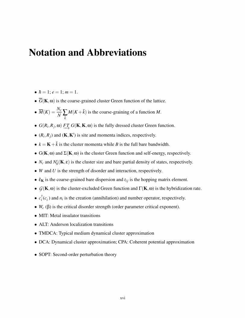
Notation and Abbreviations
• h = 1; e = 1; m = 1.
• G(K,ω) is the coarse-grained cluster Green function of the lattice.
• M(K) =Nc
N∑k
M(K+ k) is the coarse-graining of a function M.
• G(Ri,R j,ω) FT−→ G(K,K,ω) is the fully dressed cluster Green function.
• (Ri,R j) and (K,K′) is site and momenta indices, respectively.
• k = K+ k is the cluster momenta while B is the full bare bandwidth.
• G(K,ω) and Σ(K,ω) is the cluster Green function and self-energy, respectively.
• Nc and Nc0(K,ε) is the cluster size and bare partial density of states, respectively.
• W and U is the strength of disorder and interaction, respectively.
• εK is the coarse-grained bare dispersion and ti j is the hopping matrix element.
• G(K,ω) is the cluster-excluded Green function and Γ(K,ω) is the hybridization rate.
• c†i (ci ) and ni is the creation (annihilation) and number operator, respectively.
• Wc (β) is the critical disorder strength (order parameter critical exponent).
• MIT: Metal insulator transitions
• ALT: Anderson localization transitions
• TMDCA: Typical medium dynamical cluster approximation
• DCA: Dynamical cluster approximation; CPA: Coherent potential approximation
• SOPT: Second-order perturbation theory
xvi
Abstract
This work is devoted to the development of a systematic method for studying electron localization.
The developed method is Typical Medium Dynamical Cluster Approximation (TMDCA) using
the Anderson-Hubbard model. The TMDCA incorporates non-local correlations beyond the local
typical environment in a self-consistent way utilizing the momentum resolved typical-density-of-
states and the non-local hybridization function to characterize the localization transition.
For the (non-interacting) Anderson model, I show that the TMDCA provides a proper descrip-
tion of the Anderson localization transition in one, two, and three dimensions. In three-dimensions,
as a function of cluster size, the TMDCA systematically recovers the re-entrance behavior of the
mobility edge and obtains the correct critical disorder strength for the various disorder configura-
tions and the associated universal order-parameter-critical-exponent β and in lower-dimensions,
the well-knowing scaling relations are reproduced in agreement with numerical exact results. The
TMDCA is also extended to treat diagonal and off-diagonal disorder by generalizing the local
Blackman-Esterling-Berk and the importance of finite cluster is demonstrated. It was further gen-
eralized for multiband systems.
Applying the TMDCA to weakly interaction electronic systems, I show that incorporating
Coulomb interactions into disordered electron system result in two competing tendencies: the
suppression of the current due to correlations and the screening of the disorder leading to the ho-
mogenizing of the system. It is shown that the critical disorder strength (WUc ), required to localize
all states, increases with increasing interactions (U ); implying that the metallic phase is stabilized
by interactions. Using the results, a soft pseudogap at the intermediate W close to WUc is predicted
independent of filling and dimension, and I demonstrate in three-dimensions that the mobility edge
is preserved as long as the chemical potential, µ, is at or beyond the mobility edge energy (ωε). A
xvii
two-particle formalism of electron localization is also developed within the TMDCA and used to
calculate the direct-current conductivity, enabling direct comparison with experiments.
Note significantly, the TMDCA benchmarks well with numerical exact results with a dramatic
reduction in computational cost, enabling the incorporation of material’s specific details as such
provide an avenue for the possibility of studying electron localization in real materials.
xviii
Chapter 1
Structure of Dissertation
The overall aim of this dissertation is to develop a formalism capable of properly characterizing
disordered electron systems including disordered systems with off-diagonal disorders, and compet-
ing diagonal disorder and Coulomb interactions in one, two, and three dimensions. The developed
method is the typical medium dynamical cluster approximation (TMDCA) and it has been applied
to study diverse disorder configurations. Even though there is remarkable amount of works already
in the current literature employing computational techniques of varying complexity for studying
disordered electronic systems and its variants, there are still many glaring issues that are not prop-
erly understood. I will explain this assertion in details in Chapter 2.
I will give a general Introduction in Chapter 2. Here, key concepts of disorder, interactions,
the general concept of quantum transport, the scaling theory of localization based on the single-
parameter theory, and the justification for using the typical density of states as an appropriate order
parameter for characterizing not just disordered system, but when both disorders and interactions
are present at the same time, will be discussed. Most significantly, I will show from physical point
of view based on multifractal analysis that geometrical averaging of the disordered system is a
robust representation of the most probable (typical) value.
In Chapter 4, I will give an insight into the different models for studying disordered and/or
interacting electronic system. Emphasis will be on the models used in this dissertation. The local
typical medium theory will also be discussed here and its deficiencies will be given. I will in
Chapter 5 give the details of the typical medium dynamical cluster approximations (TMDCA). I
will further discuss the steps in formulating a proper TMDCA for characterizing localization in
electronic systems especially, the issue of cluster self-averaging and how to avoid it. The self-
consistency and implementation of the TMDCA will also be discussed.
1
After the above introductory and formalism development in Chapters 2 to 3, this dissertation
falls naturally into five parts, which are relatively independent:
• Study of the disordered electron system in lower (one and two) and three dimensions will be
given in Chapters 6 and 7, respectively.
• The application of the dynamical cluster approximation (DCA) and the typical medium DCA
to the study of both diagonal and off-diagonal disorder will be presented in Chapter 8.
• In Chapter 9, I will present the results for the generalization of the TMDCA for the study of
the disordered multi-band system and then present the study of a two-band species.
• The results of the initial effects electron interactions on disordered electronic systems will be
presented in Chapter 10.
• To make connection with experiments, I will in Chapter 11, present a two-particle formula-
tion that will be used to calculate the direct current conductivity within the typical medium
dynamical cluster approximation.
• Some key information that will aid in the general understanding of the dissertation are pre-
sented in Appendices B–E.
2

Chapter 2
General Introduction
2.1 Introduction
The property of some materials being conductors and others not is one of the highly researched
areas of condensed matter physics. Many experimental studies show that a slight variation of an
external parameter like pressure, chemical composition, temperature, etc., can induce a metal-
insulator-transition, i.e., turning a highly conducting metal into an insulator and vice-versa. A
phenomenon referred to as electronic localization. The physics of electron localization remains
one of the most intriguing concepts in modern condensed matter and material physics commu-
nity. Generally, a well-defined metal-insulator-transition (MIT) is observed in three-dimensional
systems even for the non-interacting electrons, as demonstrated by the single-parameter scaling
theory [4]. The physics, however, is drastically different in lower (one and two) dimensions as the
single-parameter scaling theory of localization (SPSTL) predicts the absence of delocalized phase
for the non-interacting electrons. The problem of electron localization is even more interesting in
the two-dimensions systems since it is the lower critical dimension for the Anderson localization
transitions. As a consequence of this, key interest is to use the two-dimensional system to assist
in understanding the physics of strongly correlated quasi-2D systems, such as high-Tc supercon-
ductors. Several authors (see e.g., Refs [5–11]) especially, at half-filling for the two-dimensional
system have carried out extensive theoretical and numerical studies to explore the possibility of a
metallic phase. Most of these results generally agree that in the absence of any symmetry breaking
field, the two-dimensional system is always localized. While the above descriptions of the physics
of electron localization are at half-filling, the situation seems to be different away from half-filling.
For the Hubbard model, while a strong repulsive Hubbard interaction can induce a phase transition
3
in a three-dimensional, non-disordered systems at half-filling from a metal to insulator, away from
half-filling, it remains metallic [5, 12–14].
The central question in the two-dimensional systems is whether Coulomb interactions can in-
duce a metal-insulator transitions by enhancing the conductivity of an interacting disordered sys-
tem. This conjecture is supported by experiments, which showed that interactions or any symmetry
breaking field could induce an insulator-metal transition, and hence are very important. Early ex-
periments on thin films and mesoscopic Aharonov-Bohm experiments on disordered rings demon-
strated the validity of the coherent backscattering effects in two dimensions [15–17]. Ma and
Fradkin using 1/N expansion in 2+ ε dimensions found a new “interacting” fixed point in their
study on localization and interactions in a disordered electron gas [18]. Subsequently, Finkel’stein
and co-workers, using renormalization group arguments, predicted the existence of a quantum
critical point in two dimensions (2D) [19]. The SPSTL [4] was modified into a two-parameter
scaling theory [19], the validity of which was confirmed by experiments in 2D Si-metal-oxide-
semiconductor field-effect transistors [20]. Several other authors [21, 21–28] supports that repul-
sive electron interactions can enhance the conductivity of an interacting disordered electron system
in two-dimensions leading to an MIT. The main problem in detecting a clear metal-insulator transi-
tions in two-dimensions in numerical studies have largely been due to the fact that the localization
length grows exponentially [5, 29] making it difficult to distinguish the localized phase from the
extended ones.
In three-dimensions, the pioneering work of Altshuler and Aronov, employing perturbation
theory to the lowest order in U and ignoring all crossing diagrams showed that interactions can
induce a square-root singularity at the Fermi level and hence strongly renormalize a disordered
Fermi liquid [30]. Recent work using exact diagonalization predicts a robust zero-bias anomaly
in the strong coupling, large disorder regime [31]. Quantum Monte-Carlo (QMC) [32, 33] and
renormalization group techniques [34] both show no evidence of a metallic phase in one-dimension
even in the presence of Coulomb interactions.
4
2.2 General Concepts of Disordered Systems
The understanding of the electronic and related properties of strongly correlated electron systems
are one of the most important problems in condensed matter physics. Strongly correlated systems
are challenging and comprises a wide class of materials (not limited to the transition metal oxides)
with unusual (often technologically useful) properties. It remains one of the most intensively stud-
ied areas of research in current condensed matter physics. While no single, generally acceptable
definition can be ascribed to the term strongly correlated electronic materials, it can be loosely
said to mean the behavior of electrons in materials that is generally not well described by sim-
ple one-electron models or theories such as the Hartree-Fock theory or the generally used density
functional theory and its variants.
Fundamental structures of strongly correlated materials are made from simple building blocks.
They have electronic degrees of freedom that produce exotic properties. For example, in materials
with poor screening properties, such as the doped transition metal oxides, the interaction energy
between valence electrons can overwhelm their kinetic energy, causing a strongly coupled many-
body ground state. As a result of this strong electron correlation, these materials display a range
of emergent properties, including high-temperature superconductivity (that can conduct electric-
ity without any resistance below a critical temperature), spintronics (also known as the magnetic
semiconductors that have the possibility to manipulate both the spin and the charge degrees of
freedom), exotic phases, the heavy fermions (with effective electron mass greater than its bare
mass), colossal magnetoresistance (materials that can induce a change in the resistivity by orders
of magnitudes due to the application of a few Tesla’s magnetic field), and an extreme sensitivity
to external perturbations (e.g., magnetic field or doping). Due to many competing phases (spin,
charge, lattice, and orbital degrees of freedom) involved in these systems, many complex phases
can emerge. Collective states of these complex systems are generally hard to understand by using
quantum mechanical single-quasiparticle approximation. While these various degrees of freedom
can be fine-tuned via external parameters to produce new materials and even improve on already
existing ones, such exotic electronic orderings, frequently observed in strongly correlated electron
5
systems, remain poorly understood. Understanding the properties of strongly correlated systems
remain a “Grand Challenge”. These materials do not obey the conventional laws of solid state
physics as such, new “smart” ideas are highly needed. We are, therefore, faced with two options:
to radically amend the existing laws of physics or to abandon them, and come up with new ones.
The fundamental parameters controlling the behavior of correlated systems are the hybridiza-
tion (escape) rate (a measure of the tunneling amplitude of particle hopping between sites), on-site
Coulomb repulsion energy, and the density of charge carriers or the filling factors. Disordered elec-
tron systems including the competition between disorder and interactions provide a good yardstick
for exploring some of the exotic properties of (strongly correlated) electron systems especially
since disorder is ubiquitous and unavoidable. The interplay of disorder [4, 35–37] and Coulomb
interactions [38, 39] is an important problem in diverse fields not limited to the physics of cold
atoms, photonic and bosonic systems, and optical lattices [40–43]. It has been actively studied
both theoretically [17, 28, 44–50] and experimentally (see for e.g., the metal-insulator transition
of doped semiconductors [39, 51–53] and some perovskite compounds [54–58]) for the past few
decades.
Further, exact numerical computations have been of tremendous assistant in elucidating the
properties of disordered systems as they have been successfully used to study localization. How-
ever, these exact numerical methods are severely limited. They require rather a large cluster and al-
most all known popular numerical methods, including the transfer-matrix, Kernel polynomial, and
exact diagonalization methods are difficult (almost impossible) to incorporate interactions (even an
interaction as simple as a single impurity coupling) as such, eliminates the possibility of incorpo-
rating chemically specific details. An alternative approach is offered by mean-field theories such
as the coherent potential approximation and its extensions. They generally map the lattice onto
a relatively small self-consistently embedded clusters and these methods have been successfully
extended to the treatment of interactions as well as disorder and to chemically realistic models. Un-
fortunately, these methods have been woeful in the treatment of Anderson localization due mainly
to the averaging procedure utilized and improvements in the environment describing the effective
medium have been limited to single sites.
6
The difficulty in formulating a mean-field theory for studying strongly correlated systems are
easy to guess. The two limits: a good metal and a good insulator and the intermediate regime, are
generally very different physical systems that can be characterized by subtle elementary excitations
with different energy scales. For insulators, these are long-lived (collective) bosonic excitations
such as spin waves and phonons; and for metals, they are generally quasiparticles similar to the
electrons are excited above the Fermi sea. At the intermediate regime of the metal-insulator transi-
tions (MIT), both types of excitations coexist leading to a non-trivial density of states. As such, a
“simple” theoretical formalisms fail as they are not capable of distinguishing between the delocal-
ized and localized phases in the gapless single-particle spectra of the correlated Anderson insulator.
Conceptually, these are features of a typical quantum critical point (QCP) but with an additional
bottleneck. Taking a typical QCP involving spin or charge ordering as an example, the criticality
can easily be described by examining the fluctuations associated with the order parameter due to an
appropriate symmetry breaking. This is strikingly different in the case of the MIT since it is more
suitably described as a dynamical transition and a straightforward order parameter theory is not
available. As a consequence of these, the intermediate regime between the metal and the insulator
has remained very hard to understand both from the practical and conceptual standpoint.
2.3 Fundamentals of Quantum Transport
The phenomenon of localization transition is a typical example of quantum transport where co-
herent multiple backscattering interference effects of electron states propagating in a disordered
medium may inhibit their propagation across the sample. To understand how this happens, it is
intuitive to describe the manifestation of quantum interference in good metals with the disorder.
The basic microscopic ideas of quantum transport are quite understood [59,60]. As emphasized by
Schrödinger, the four noble truths about quantum states are superposition, interference, nonclon-
ability and uncertainty (no quantum copier machine), and entanglement [61, 62]. The scattering
of electrons off a random impurity can be characterized by three energy-dependent length scales
vis-à-vis three energy-dependent time scales (τ(k) = l/υ, where υ =kε(k), ε(k) is the dispersion
7

relation). For a single electron scattering off impurity states, the renormalized k-wave states can
be described as quasiparticles in the proximity of the impurity states with a finite lifetime τs(k).
Hence, single scattering processes define the first length scale, known as the scattering mean-free
path, ls = υsτs which is the typical length an electron travels before it loses the memory of its initial
state. It generally describes the decay length of the average single-particle Green’s function [63].
The multiple scattering processes defines the second length scale in the scattering of electrons
in a disordered medium. This length scale characterizes the typical length scale traveled by the
electrons before losing the memory of its initial direction. This length scale is generally known as
the transport (Boltzmann) mean-free path, lB. The fundamental difference between ls and lB is that
the latter is the length over which the momentum transfer becomes uncorrelated and involves extra
factor (1− cosθ) [63]. It is an important length scale in the description of Anderson localization
transition (ALT). It is directly proportional to the multiple backscattering processes that drive ALT
where in general within the lB, the ballistic electron trajectories become diffusive. In general,
lB > ls, but are equal in the white-noise limit (here wavelength is smaller than the typical size of
the impurities), and the disorder can be said to be a set of randomly distributed Dirac peaks [64]
with an isotropic scattering (the so-called isotropic limit is a case where there is no p-spherical
harmonic and the cosθ averages to zero). In this limit, the electron loses simultaneously, the
memory of its initial state and initial direction of propagation.
While the Boltzmann mean-free path lB characterizes the typical length scale traveled by the
electrons before losing the memory of its initial direction, it does not define the length scale of the
return of the electrons to its initial state as embedded in the return probability of the electrons on site
l after time τ, P(τ) =⟨|G(l, l,τ)|2
⟩, where G(l, l,τ) is the local Green function. Diffusive transport
permits the electrons return to their initial positions via loop paths in a ‘constructive’ interference
setting. Since each of the loops can be traveled in either way, two multiple-scattering paths with
exactly the same phase develops during a successive scattering process. The coherent nature of the
above described scenario, which is generic for any disordered potential guarantees that it survives
disorder averaging. Also, the coherent nature of the multiple-scattering processes ensures that
the two paths are in phase and hence ‘constructive’ interference which significantly enhances the
8
return probability of the electrons. This generally leads to the well-known coherent backscattering
and hence localization. In cases where the coherent backscattering is in the presence of nominal
disorder strength, weak localization with significant diffusive transport exists [36]. However, in
the strong disorder regime, the diffusive transport is completely quenched, a scenario referred
to as strong or Anderson localization [35, 65]. At this point, the probability distribution of the
electrons exhibit spatially exponential decay. This defines the third typical length scale known as
the localization length, lτ which defines the ALT.
9
Chapter 3
Metal Insulator Transitions
In this Chapter, I will give a brief review of the various mechanisms described in details in Chap-
ter 4 that are the major players in the localization of electron systems. Generally in fermionic
systems, there are two basic routes to electronic localization: randomness (or disorder) generally
referred to as the Anderson localization or due to electron interactions known as the Mott localiza-
tion transitions. At this point, it is important to make distinction between metal-insulator transitions
and other forms of transitions that occur in materials. The metal-insulator transitions is a phase
transition strictly occurring at zero temperature T = 0. As such, it is a quantum phase transition.
A material is a metal when the direct current (DC) conductivity σ(T ) remains finite as T → 0 and
it is an insulator, when σ(0) = 0. Hence, the electron localization in this sense involve a transition
from a delocalized to localized states, and vice-versa. In contrary, band-like transitions [66, 67]
as in Bloch transitions are due to energetic separation of initially overlapping bands or the Perls
transitions [68], which is due to lattice distortion.
3.1 Ideal Material: Perfect Crystal System
The perfect periodicity in real solids is an idealization rather than a rule. In general, there are
imperfections in real materials and are of great importance for transport properties. The broken
translational symmetry makes the system deviate from the extended Bloch wave nature, and in
some cases, to localized states. As such, model of ordered systems cannot be used to understand
disordered materials [69]. The problem of quantum localization in a random potential (commonly
known as Anderson localization [35]) has proven to be surprisingly rich and remains one of the
most fascinating mesoscopic phenomena (for a review, see Refs. [44, 60, 69, 70]) in condensed
10

matter physics. In spite of the overwhelming collective effects of the scholarly researchers, the
problems associated with Anderson localization are recently understood and the phenomenon con-
tinues to generate new ideas.
In general due to computational or experimental limitations, the disorder is usually viewed as
non-desirable, and may be neglected in order to deal with generic models. In most cases, this
approach is often successful in describing macroscopic properties where microscopic disorder is
treated as a source of uncertainty in physical measurements. However, it is now well-known that in
some cases, a disorder can have dramatic effects even at the macroscopic scale [46,69,71,72]. An
emblematic and fascinating example is Anderson localization, in which disorder can turn a piece
of metal into an insulator; and as explained above, a typical disorder configurations may locally
favor one or another of the many competing “exotic” phases of matter.
3.2 Anderson Localization Transitions
The Anderson localization transitions are basically induced by disorder (or randomness). As ex-
plained in Chapter 2, Section 3.1, the idea of a perfect crystal is an idealization. Real materials
inevitably contain one form of disorder or other forms of lattice imperfections and/or disorder [36]
and the presence of disorder can dramatically alter the Bloch states, which is always extended.
Disorder-driven metal-insulator-transitions remains one of the most fascinating and studied phe-
nomena in disordered systems not limited to the “traditional condensed matter physics commu-
nity” but have actively been studied in other fields [35, 40–43, 73–94]. As has been previously
explained in Chapter 2 Section 3.5, the dynamics of Anderson localization transitions rely on co-
herent backscattering due to the restoration of coherent phase (interference effects). This effect
if sustained alters the eigenmodes of the electrons in the system from extended to localized states
due to the trapping of electrons into long-lived resonant states. The ALT is characterized by the
vanishing of the hybridization paths accompanying the quantum localization of the wavefunctions
as a consequence of the coherent backscattering off random impurities. Here, the charge carriers
do not generally vanishing and no opening of a gap in the single-particle spectra.
11
While Anderson localization will be highlighted in most part of this dissertation as it is one
of the main topics being investigated, it is imperative to note that the Anderson metal-insulator-
transitions is quite different from the metal-insulator-transitions (MIT) that occurs in periodic sys-
tems. In the latter, only partially, filled bands carry current, i.e., there is a gap opening in the single
particle spectra even if all states are extended [95] while in the former, at the transition, the spectra
is gapless [96] and no current propagates through the entire system. 1
The Anderson localization transition is normally manifested as the impeding of electronic diffu-
sion and hence, localized states emerges whose properties are described by a characteristic length,
localization length (cf. Chapter 4 Section 2.3) that determines the degree of localization [36, 93].
At an intermediate stage of electron diffusion (weak disorder), localization is weak and acts as a
precursor to Anderson (strong) localization [36, 44, 94]. An avalanche of research following the
1958 seminal paper of Anderson [35] has explored many aspects of localization transitions, all
generally with the same aim of trying to understand the role of disorder in materials. As search
for new improved materials continues, key fundamental questions among the various open issues
in characteristic disordered systems are to understand the role of disorder and how to effectively
control localized modes in achieving metal-insulator-transitions. The ability to understand this
phenomenon is not only important in our quest for new insights on the dynamics of electronic
localization, but will aid in identifying new areas of applicability of disordered systems.
3.3 Mott Localization Transitions
A system with dominant electron correlation as compared to the kinetic energy, undergoes a tran-
sition from a metal to a correlation-induced insulator. This is generally referred to as the Mott
MIT [38, 51] where electrons are localized (trapped) in their individual atomic orbitals leading
to the opening of a gap in the single-particle spectra. The study of MIT in the so-called cor-
related systems came to a renewed interest in the last few decades, following the discovery of
high-temperature superconductivity (for recent studies and reviews, see Refs. [99–101]).
Assuming a crystal with one valence electron per atom, then, the opening of the gap following
1The density of states of Anderson localized state is uncritical at the transitions but the local density of states is critical [2, 36, 97, 98].
12

Mott transition is due to the competition between the kinetic energy gained by the delocalization
of the electron and the activation energy emanating from the creation of electron-hole pair induced
by the Coulomb interaction. Unlike the disorder induced metal-insulator-transitions (MIT), the
interaction induced MIT is not ’fully’ a single-particle mechanism since according to the single-
particle picture, a predicted metallic system can become insulating due to electrostatic inter-particle
interaction.
Most of the diverse exotic behaviors in correlated materials can be traced to the electron inter-
actions [8, 102–104]. For an insight to the above assertion, we recall that in conventional metals
electrons barely interact with each other. In the language of the Fermi liquid theory, there is the
tendency to screen local charges such that electrons can be treated as isolated particles in a ho-
mogeneous background known as Fermi sea. In contrast, in the presence of electron correlations,
these electrons start to interact with each other. This scenario lacks any broadly successful the-
oretical formalism modeling the behavior. Hence, conventional approaches and/or ideas proved
of little significance. However, recent breakthroughs both from experimental and theoretical per-
spective [52, 60, 105, 106] have led to the avalanche of new and exciting techniques which have
enhanced our understanding of the general problem of metal-insulator transitions in correlated
materials.
3.4 Disorder and Electron Correlations in Materials
A system with a combined disorder and electron interactions no doubt is more challenging to char-
acterize [44, 69, 104] than when disorder or interactions act independent of each. This is a typical
characteristic of real materials. Real materials are always characterized by some electron corre-
lations and numerous kinds of disorder, such as impurities; interstitials, antisites, and topological
defects; vacancies, inhomogeneous chemical distribution, and/or nonstoichiometric composition;
etc. that give rise to subtle many-body phenomena [30, 44, 46]. In essence, disorder can be said to
be ubiquitous, and, in fact, disorder and electron correlation inevitably coexist. Therefore, it is im-
portant to properly understand the combined effects of disorder and electron interaction. Naively,
13
since both randomness and Coulomb interactions can independently lead to MIT, one would expect
their combined effect to be complimentary in inducing MIT. In general, the opposite has been ob-
served to be the case. Interacting disordered electron systems show strong renormalization of the
disorder strength [8]; and concomitant increased inelastic scattering and hence reduction in the ef-
fective disorder strength [60] that may inhibit the development of the quasi-coherent energy scale,
already in the metallic state [102]. As a consequence of this, there will be non-trivial renormal-
ization of the trajectories of the mobility edge and the critical parameters like the critical disorder
strength may be different from those of the “pure” Anderson MIT [12].
While there have been significant efforts to understand the combined effect of disorder and in-
teractions on the local density of states close to the Fermi level, the band edges have received scant
attention. Specifically, the effect of weak interactions on the mobility edge has not been discussed
thus far. This can be attributed to the difficulty in defining a proper mean-field order parameter ca-
pable of distinguishing between the delocalized and localized phases in the gapless single-particle
spectra of the correlated Anderson insulator. The presence of interaction will further complicate
this already intricate situation due to the quantitatively, different, low energy scales under this co-
existence with a nontrivial density of states (DoS) of the Anderson and Mott insulators. This is
one of the main issues being addressed in this dissertation, which is to systematically study the
initial effects of electron interactions on the single-particle excitation; the mobility edge trajecto-
ries (the energy separating extended and localized electron states); and the critical behavior of the
localization transition of a disordered electron system.
We note that in the past decades, some theoretical and experimental efforts have been made to
study the coexistence of disorder and interaction [8,49,55,60,107]. However, unlike these previous
computational methods, the results presented here incorporates both nonlocal spatial correlations
(by using the newly developed TMDCA [2]) and onsite electron interactions incorporated via non-
local and frequency dependent self-energy using second order perturbation theory. Also, disorder
and interaction are treated as a function of increasing cluster size as such, many “higher order”
nonlocal diagrams are self-consistently incorporated beyond a single impurity level in a typical
effective medium environment.
14
3.5 Characteristics of a Localized System
A localized electronic system has a unique property which distinguishes it from a delocalized
phase. Here, I will briefly discuss some of these unique characteristics.
3.5.1 Probability Distribution Function and Asymptotic Wavefunction
One of the most important parameter characterizing a localized electronic system is its probability
distribution function (PDF) [35]. This is manifested in the complex wavefunction, which generally
has a multifractal structure with large amplitude variations in space [37]. Before an electronic
system becomes localized, the amplitude of the wavefunction is approximately the same on every
site vis-à-vis, the probability distribution function of the local density of states is symmetric with a
Gaussian distribution. However, at the localized phase, the wavefunctions have substantial weight
on a few sites only, falling off exponentially at large distances with the PDF of the local density
of states developing long tails and are extremely asymmetric with a log-normal shape [65]. Most
of the weight is concentrated around zero. More precisely, the wavefunction ψα(x) for any given
eigenstates |ψα〉 of the Hamiltonian H behaves as [97]
|ψα(x)| ∼ e−|x−x(α)0 /ξ (3.1)
where ξ ≡ ξ(ωα) is the characteristic localization length, which determines the asymptotic behav-
ior of ψα(x), when |x| → ∞ and x(α)0 is the center of the localization of state |ψα〉.
3.5.2 Coherent BackScattering
As explained above, one of the essential ingredients for achieving (weak) localization of electrons
is the coherent backscattering. Heuristically, the Feynman paths [30, 108, 109] depict the best way
to look at the coherent backscattering [35].
Assuming a good conductor (λ ≪ l), moving from point A to B, with the multiple scattering
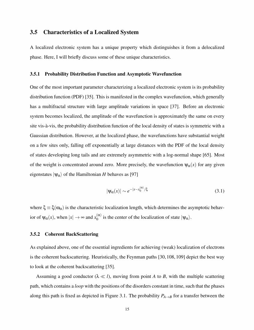
path, which contains a loop with the positions of the disorders constant in time, such that the phases
along this path is fixed as depicted in Figure 3.1. The probability PA→B for a transfer between the
15
α
βθα
θβd
Figure 3.1: Left panel: Possible Feynman paths for a particle to move from point A to B. ’O’ de-
notes point of path self-crossing, which are identical under time reversal. Right panel: Expanding
points A to B showing the Coherent backscattering process.
two points can be obtained by squaring the modulus of the sum of the various amplitudes of the
probability of the particle to pass through all the possible paths given as
Pα→β∼α =
∣∣∣∣∑
α
Aα
∣∣∣∣
2
(3.2a)
|Pα→β|= ∑α
|Aα|2 + ∑α6=β
AαA∗β = |Aαeiθα +Aβeiθβ|2 = A2
α +A2β +2AαAβ cos(θα −θβ)
︸ ︷︷ ︸
=1 for θα=θβ
. (3.2b)
where Aα is the probability amplitude of the Feynman path α. Equation 3.2a depicts the sum of
the probabilities of a particle to pass any direction while Equation 3.2b incorporates the interfer-
ence of the various amplitudes. The physical interpretation of Equation 3.2a is that for most of
the paths, interference is destroyed since their lengths differ strongly leading to the wavefunction
having different phases on these paths. Hence, these different phases basically cancel out when
summed over the various paths. This leads to a classical description of electrons (Boltzmann or
diffusive transport). However, if the system is symmetric under time reversal, there are paths of a
special kind (self-intersecting paths). Consider two paths A (clockwise) and B (anti-clockwise) (cf.
Figure 3.1(a)). Then, for each path Aα (α), there exists exactly one path Aβ (β), which is the time
reversal counterpart of Aα (α) (cf. Figure 3.1(b)). Since these two paths are coherent, hence, in
phase, their interference cannot be neglected. Their return probability is thus twice as large as the
classical counterpart (cf. Equation 3.2b), and this corresponds to quantum corrections to electron
16

transport as manifested in the conductivity. Letting Aα = Aβ = A, Equation 3.2 becomes
Pα→β =
4A if θα = θβ in phase
2A if θα 6= θβ out of phase
(3.3)
Thus, localization occurs when there is phase coherency in the multiple backscattering trajec-
tories of the electrons with a return probability to their original positions vis-à-vis, the electrons
remain at their sites. 2 Since the total probability is normalized, i.e.,
∑β
Pα→β = 1 (3.4)
the quantum correction to the classical (diffusive) regime generally leads to enhanced return proba-
bility and hence, reduction to the ability of the particle to propagate [30,108,110] corresponding to
a reduction in the conductivity of the system. In 3D where there is broad MIT, the return probabil-
ity is weak and continually decreases with increase in energy such that localization only manifests
at sufficiently low energy. This particular picture leads to the development of the mobility edge
which separates the diffusive states (klB & 1) from the localized states (klB . 1).
3.5.3 Lifshitz Tails
The Lifshitz tails [97, 111] is one of the signatures of a localized state. It has its origin from the
emergence of rare configurations of on-site energies with eigenenergies close to the mobility edge
spectrum [97,111,112]. The Lifshitz states generally emerge, when the disorder strength is strong
such that particles with high(low) energies as compared to the average disorder potential are bound
within the hills(valleys) of the energy landscape. This is a highly non-trivial quantum effect due to
slowly diffusive tunneling by the particles.
Consider the eigenenergies ω ∼ ω±0 of the eigenstates H (ω±
0 ∼ ±(εi+2td) is the upper(lower)
boundary of the energy of H). This energy scale can only exist when all the on-site energies εi are
2A note of caution though in low dimensional systems (1 and 2D), the concept of diffusion being a precursor for ALT is strictly not true since,
in general, in these dimensions, all states are localized for any arbitrary disorder strength [4] in the absence of any symmetry breaking field.
17
at a small regime very close to the boundary (edge) of the energy distribution [97, 111]. 3 Hence,
states with energies close to the edge (top and bottom of the bands) are strongly localized within
this regime due to strongly fluctuations. The probability of finding such rare configurations within
a finite region of the lattice is exponentially small.
3.5.4 Mobility Edge
As has been explained in the previous sections, all single-particle spectra become localized above
a certain critical value of the disorder strength Wc. However, even before all the states become
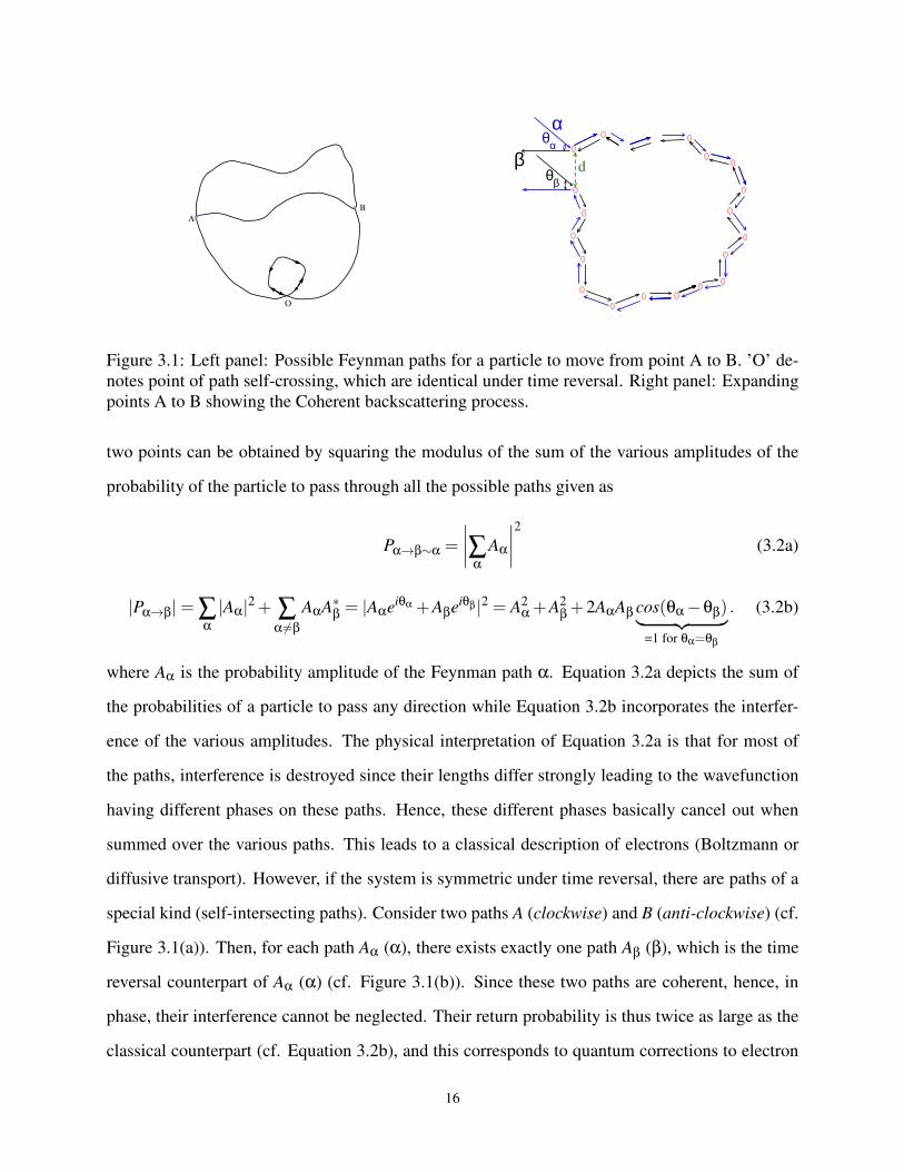
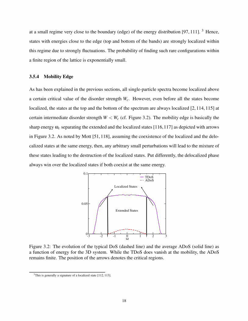
localized, the states at the top and the bottom of the spectrum are always localized [2, 114, 115] at
certain intermediate disorder strength W <Wc (cf. Figure 3.2). The mobility edge is basically the
sharp energy ωc separating the extended and the localized states [116,117] as depicted with arrows
in Figure 3.2. As noted by Mott [51, 118], assuming the coexistence of the localized and the delo-
calized states at the same energy, then, any arbitrary small perturbations will lead to the mixture of
these states leading to the destruction of the localized states. Put differently, the delocalized phase
always win over the localized states if both coexist at the same energy.
-3 -2 -1 0 1 2 3ω
0
0.05
0.1TDoSADoS
Extended States
Localized States
Figure 3.2: The evolution of the typical DoS (dashed line) and the average ADoS (solid line) as
a function of energy for the 3D system. While the TDoS does vanish at the mobility, the ADoS
remains finite. The position of the arrows denotes the critical regions.
3This is generally a signature of a localized state [112, 113].
18
3.6 The Scaling Theory of Anderson localization Transition
One of the features of Anderson localization is that it is characterized by eigenvalues that are
infinitely close to each other, and eigenfunctions that are exponentially localized. Of course, the
above description of Anderson localization is more or less a mathematical abstraction as it is not
of much usefulness to an experimentalist trying to characterize a localization transitions since, in
general, no one can actually measure eigenfunctions in localized realistic systems. The foundation
of what is known today as the scaling theory of Anderson localization was by the earlier works of
Landau [119] who observed that the transport in the localized regime of a finite system is described
by the conductance, G rather than the conductivity, σ as one would generally expect.
G = σLd−2 (3.5)
where d is the dimension of the system.
In some of the earlier works on disordered electron system by Thouless [70,120], he showed that
in a finite open media, eigenvalues are repelled by quantization criterion. However, due to leakage
through the boundaries, the system achieves a finite width. Further, Thouless and co-workers [70,
120–123] demonstrated that the localization transition occurs when the level separation (the energy
related to the average diffusion time a particle needs to propagate through the volume, also known
as the Thouless energy,
ET = h/τφ (3.6)
where τφ = Lφ/D is the dephasing or Thouless time, and D is the microscopic diffusion constant)
is larger than the level width (the averaged energy spacing of two neighboring eigenenergies in the
volume, ∆Es). From Einstein relations,
σ = e2N(εF)D (3.7)
where e is the electronic charge, N(εF) is the density of states at the Fermi energy. Combining the
19
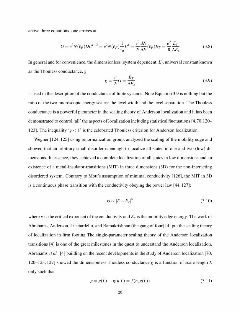
above three equations, one arrives at
G = e2N(εF)DLd−2 = e2N(εF)1
τφLd =
e2
h
dN
dE(εF)ET =
e2
h
ET
∆Es
(3.8)
In general and for convenience, the dimensionless (system dependent, L), universal constant known
as the Thouless conductance, g
g ≡ e2
hG =
ET
∆Es(3.9)
is used in the description of the conductance of finite systems. Note Equation 3.9 is nothing but the
ratio of the two microscopic energy scales: the level width and the level separation. The Thouless
conductance is a powerful parameter in the scaling theory of Anderson localization and it has been
demonstrated to control ‘all’ the aspects of localization including statistical fluctuations [4,70,120–
123]. The inequality ‘g < 1’ is the celebrated Thouless criterion for Anderson localization.
Wegner [124, 125] using renormalization group, analyzed the scaling of the mobility edge and
showed that an arbitrary small disorder is enough to localize all states in one and two (low) di-
mensions. In essence, they achieved a complete localization of all states in low dimensions and an
existence of a metal-insulator-transitions (MIT) in three dimensions (3D) for the non-interacting
disordered system. Contrary to Mott’s assumption of minimal conductivity [126], the MIT in 3D
is a continuous phase transition with the conductivity obeying the power law [44, 127]:
σ ∼ |E −Ec|ν (3.10)
where ν is the critical exponent of the conductivity and Ec is the mobility edge energy. The work of
Abrahams, Anderson, Licciardello, and Ramakrishnan (the gang of four) [4] put the scaling theory
of localization in firm footing The single-parameter scaling theory of the Anderson localization
transitions [4] is one of the great milestones in the quest to understand the Anderson localization.
Abrahams et al. [4] building on the recent developments in the study of Anderson localization [70,
120–123, 127] showed the dimensionless Thouless conductance g is a function of scale length L
only such that
g = g(L)≡ g(n.L) = f (n,g(L)) (3.11)
20
where n is a scale factor. Equation 3.11 makes the assumption that in stacking small systems to
form a large system, that the conductance of a large system depends only on the conductance of the
original small system. The key question that needs to be addressed is how g depends on L. Recall
that for a pure metal, the conductance is generally large, g ≫ 1. In this metallic limit, we know
from Ohm’s scaling law that g ≈ σLd−2 + .... Also, in the strongly localized regime g ≪ 1, the
conductance drops off exponentially with length as g ≈ e−L/ξ, where ξ is the localization length.
One can obtain the β-function by carefully interpolating between theses two limits. This can be
achieved by using the intrinsic property of the problem. Since it basically involves doubling the
system size many times, the best way to think about it is to assume a logarithmic scale. Taking the
derivatives of the two limits described above as
d lng
d lnL= β[g(L)] =
(d−2)−ζ(1g), g ≫ 1
−1ξ
dLd lnL
=−Lξ= lng, g ≪ 1
(3.12)
where ζ is some unknown constant due to higher order corrections by assuming that there exists
an analytic expansion of β in powers of 1/g. A qualitative, schematic plot of the β-function for
the various dimensions is shown in Figure 3.3. With Equation 3.12, one can explore how β is
expected to behave in the β − g plane in one, two, and three dimensions. In one dimensions,
Figure 3.3: A schematic plot of the β for one, two, and three dimensions. For the two-dimensional
case, the dotted line shows a system with external field.
21

from Equation 3.12, neglecting the corrections, β is always negative for g ≫ 1 implying that the
conductance decreases towards 0 and eventually crashes exponentially as g becomes less than
unity in the thermodynamic limit (L → ∞). In two dimensions, the asymptotic limit of β for
g ≫ 1 can also be seen to be 0. This implies that in the thermodynamic limit, the conductance
of a two-dimensional system is independent of the system size. But the two-dimensional system
is a special case since from Equation 3.12, the leading contribution to the β-function vanishes
in the Ohmic regime. However, assuming there is a time reversal symmetry breaking field like
spin-orbit coupling or say a different universal class [128, 129] aside the orthogonal class, the
negative sign of the correction β(g)∼−1/g may change leading to a phase transitions even in two
dimensions [16, 37, 65].
In three dimensions, the situation is very different. From Equation 3.12 for g ≫ 1, the β-
function is positive, i.e., ((d − 2) = 1) while for g ≪ 1, the β-function goes like lng. The impli-
cation of this from continuity perspective is that on the g-axis, β[g] must cross the β = 0 at some
point gc. Near the transition (i.e., |(g− gc)/gc|), where one expects the linearization of β to be
valid, the localization length scales as
ξ ∼ |g−gc
gc|−1/s = |g−gc
gc|−ν (3.13)
where ν = 1/s is the critical exponent of the correlation length as well known from the theory of
critical phenomena [130]. The predictions of the single-parameter scaling have been corroborated
by numerical and theoretical studies [36, 131–133], including a generalization to two-parameter
scaling theory [19]. However, there are some numerical works reporting its violation [36, 98].
3.7 Scaling Theory of the Typical Density of States
As explained earlier, unlike the conventional continuous phase transitions, the metal-insulator tran-
sition is unique since it is more suitably described as a dynamical transitions, as such, an appro-
priate order parameter for the Anderson localization is difficult. As demonstrated in Ref. [2, 134],
the appropriate order parameter characterizing localization transition should satisfy the following
22
criteria:
1. The order parameter should vanish in the localized (or extended) phases;
2. It should exhibit power law behavior and capture the critical behavior of Anderson local-
ization transitions with the correct critical disorder strength Wc and order parameter critical
exponent, β;
3. The order parameter acquires a finite positive value in the localized (or extended) phase.
The typical density of states TDoS meets all of the above requirements and it has been demon-
strated as the appropriate order parameter for characterizing the localization transition [2]. For a
system near the critical point xc, the TDoS behaves as
T DoS ∝ (xc − x)β, ∀x < xc (3.14)
where β = ν(αo − d) is the universal order parameter critical exponent (typical order parame-
ter exponent) [135], αo is the Lipschitz-Hölder exponent [134]. In the TMDCA, Equation 3.14
is characterized by taking the TDoS at the band center while the disorder strength controls the
localization transition as
T DoS(ω = 0) = (Wc−W )β, ∀W <Wc (3.15)
From above, the TDoS will vanish at Wc as such, Equation 3.15 is only valid for W <Wc.
3.8 Justification for Typical Density of States as Order Parameter
The local density of states contains all the information about the local amplitudes of the electronic
wave functions. As such, its probability distribution functions (PDF) is a natural way to character-
ize the Anderson localization transition. Unlike the global (average) density of states, which are
not critical at the localization transitions, the (unaveraged) local density of states is critical at the
transition [35].
23
The study of disordered systems relies on the PDF of the local variables to measure ‘random’
quantities of interest [35]. To characterize localization, the most important quantity in the ma-
jority of physical or statistical problems is usually the “typical” value of the ‘random’ variable,
which corresponds to the most probable value of the PDF [136]. In most systems the nature of the
PDF is not known a priori; as such, we have limited information via the moments or cumulants
of the PDFs. Under such situation, the “typical” or the most probable value of the PDF [136]
contains important and direct information. Different from some systems where the first moment
(the arithmetic average) is a good estimate of the random variable, the Anderson localization is a
non-self-averaging phenomenon. Close to the critical point if the system is phase coherent (meso-
scopic regime), quantum interference effects cause the strong fluctuation of physical quantities
(e.g., LDoS) [137] such that corresponding PDF of the local density of states is very asymmetric
with long tails [135,138] needing infinitely, many moments to describe it [136]. In some cases, the
corresponding moments might not even exist especially close to the critical point [139].
Naturally, at the localization transitions, the typical local density of states vanishes while the
continuous local spectrum becomes sets of delta-function peaks with long-lived resonance states.
As a consequence, these long-lived resonance states at a given lattice site, acquire a finite escape
rate which, according to the Fermi Golden rule, can be approximated as [35]
τφ ∼ 1/(t2ρi) (3.16)
where t is the hopping matrix and ρ is the local density of states in the neighborhood of site i.
From Equation 3.16, it is obvious that the typical escape rate is dictated by the local density of
states (TDoS); implying that the TDoS directly measures the conductivity within the Drude ap-
proximation. Based on the above conjecture, the TDoS possess all the essential qualities of a
proper order parameter for characterizing localization transitions. In the actual computations, the
TDoS is generally approximated by the geometric value. This can be justified by noting that close
to the transition, the pertinent distribution of the TDoS becomes broad, an indication of multifrac-
24
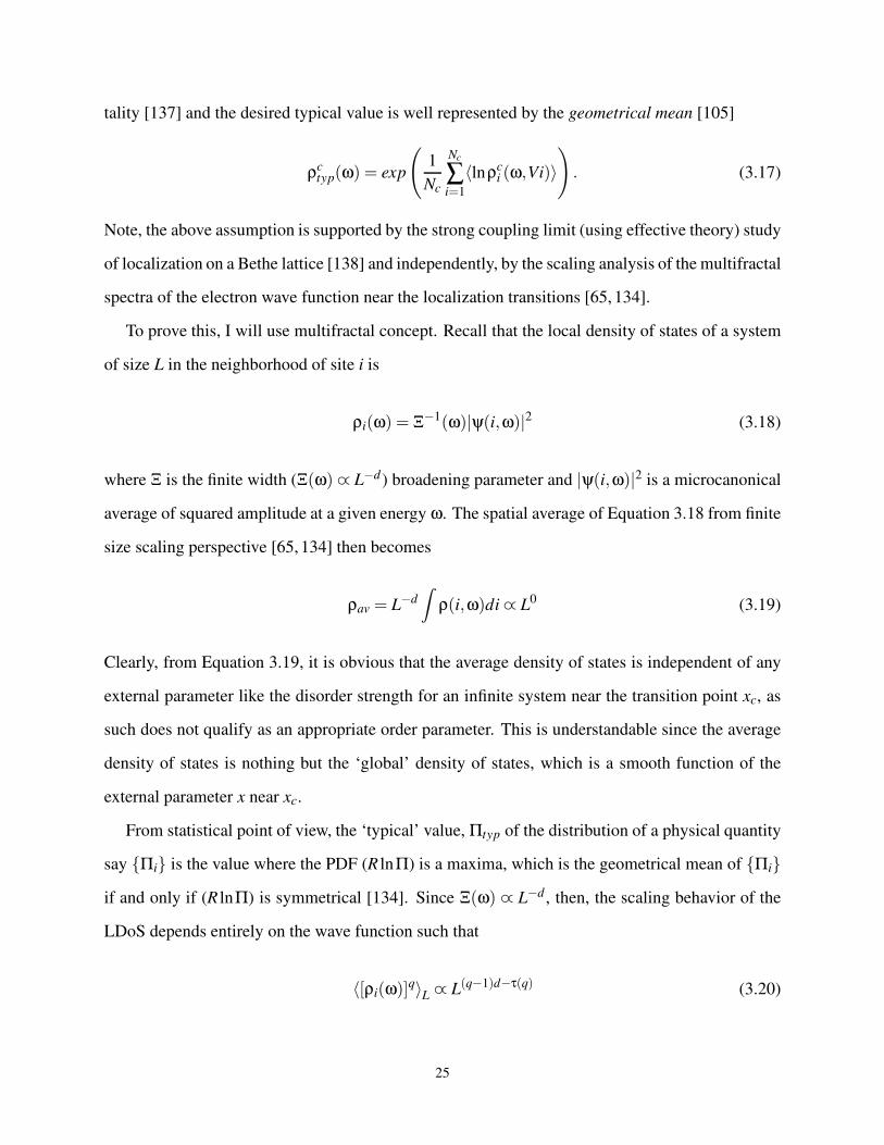
tality [137] and the desired typical value is well represented by the geometrical mean [105]
ρctyp(ω) = exp
(
1
Nc
Nc
∑i=1
〈lnρci (ω,Vi)〉
)
. (3.17)
Note, the above assumption is supported by the strong coupling limit (using effective theory) study
of localization on a Bethe lattice [138] and independently, by the scaling analysis of the multifractal
spectra of the electron wave function near the localization transitions [65, 134].
To prove this, I will use multifractal concept. Recall that the local density of states of a system
of size L in the neighborhood of site i is
ρi(ω) = Ξ−1(ω)|ψ(i,ω)|2 (3.18)
where Ξ is the finite width (Ξ(ω)∝ L−d) broadening parameter and |ψ(i,ω)|2 is a microcanonical
average of squared amplitude at a given energy ω. The spatial average of Equation 3.18 from finite
size scaling perspective [65, 134] then becomes
ρav = L−d
∫ρ(i,ω)di ∝ L0 (3.19)
Clearly, from Equation 3.19, it is obvious that the average density of states is independent of any
external parameter like the disorder strength for an infinite system near the transition point xc, as
such does not qualify as an appropriate order parameter. This is understandable since the average
density of states is nothing but the ‘global’ density of states, which is a smooth function of the
external parameter x near xc.
From statistical point of view, the ‘typical’ value, Πtyp of the distribution of a physical quantity
say Πi is the value where the PDF (R lnΠ) is a maxima, which is the geometrical mean of Πi
if and only if (R lnΠ) is symmetrical [134]. Since Ξ(ω) ∝ L−d , then, the scaling behavior of the
LDoS depends entirely on the wave function such that
〈[ρi(ω)]q〉L ∝ L(q−1)d−τ(q) (3.20)
25
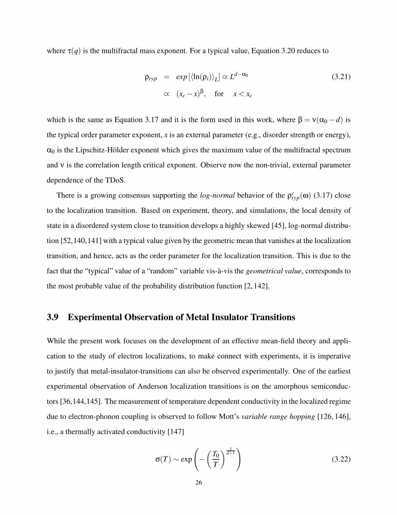
where τ(q) is the multifractal mass exponent. For a typical value, Equation 3.20 reduces to
ρtyp = exp [〈ln(ρi)〉L]∝ Ld−α0 (3.21)
∝ (xc − x)β, for x < xc
which is the same as Equation 3.17 and it is the form used in this work, where β = ν(α0 − d) is
the typical order parameter exponent, x is an external parameter (e.g., disorder strength or energy),
α0 is the Lipschitz-Hölder exponent which gives the maximum value of the multifractal spectrum
and ν is the correlation length critical exponent. Observe now the non-trivial, external parameter
dependence of the TDoS.
There is a growing consensus supporting the log-normal behavior of the ρctyp(ω) (3.17) close
to the localization transition. Based on experiment, theory, and simulations, the local density of
state in a disordered system close to transition develops a highly skewed [45], log-normal distribu-
tion [52,140,141] with a typical value given by the geometric mean that vanishes at the localization
transition, and hence, acts as the order parameter for the localization transition. This is due to the
fact that the “typical” value of a “random” variable vis-à-vis the geometrical value, corresponds to
the most probable value of the probability distribution function [2, 142].
3.9 Experimental Observation of Metal Insulator Transitions
While the present work focuses on the development of an effective mean-field theory and appli-
cation to the study of electron localizations, to make connect with experiments, it is imperative
to justify that metal-insulator-transitions can also be observed experimentally. One of the earliest
experimental observation of Anderson localization transitions is on the amorphous semiconduc-
tors [36,144,145]. The measurement of temperature dependent conductivity in the localized regime
due to electron-phonon coupling is observed to follow Mott’s variable range hopping [126, 146],
i.e., a thermally activated conductivity [147]
σ(T )∼ exp
(
−(
T0
T
) 1d+1
)
(3.22)
26
where d is the dimension. Taking three-dimension, for example, exponent in Equation 3.22
changes from 1/4 to 1/2 when Coulomb interactions between localized electrons are taken into
account as demonstrated by Efros and Shklovskii [148].
One of the most studied system exploring electron localization is the heavily doped semiconduc-
tors. Notable among them are the Si:P and Si:B [44, 143, 150–152] where some of the predictions
of the one-parameter scaling [4] were experimentally tested. In the pioneering work of Paalanen
et al. [143] on Si:P, the authors showed that the application of a uniaxial stress, which tunes the
concentration at millikelvin temperatures lead to a metal-insulator-transition (cf. Figure 3.4) with
a critical exponent µ = 0.55±0.1 [153] in contrast to the predictions of the single-parameter scal-
ing. However, more recent data where the concentration of P is varied close to MIT by Stupp et al.
[149] show similar temperature dependence of the conductivity (cf. 3.5(a)) however, the σ(0) as a
function of reduced concentration ((N−Nc)/Nc) 4 for a given concentration Nc = 3.52×1018cm−3
inferred from (cf. 3.5(a)) shows a cross-over from µ ∼ 0.5 to 1.3 as the concentration decreases
towards the critical concentration. This was attributed to the change in sign of the temperature
4Nc is used in this section to denote electron concentration. It should not be confused with the cluster size as used in other places.
Figure 3.4: The evolution of the conductivity as a function of temperature for various uniaxial
stress near MIT for Si:P. Plot is taken from Ref. [143].
27
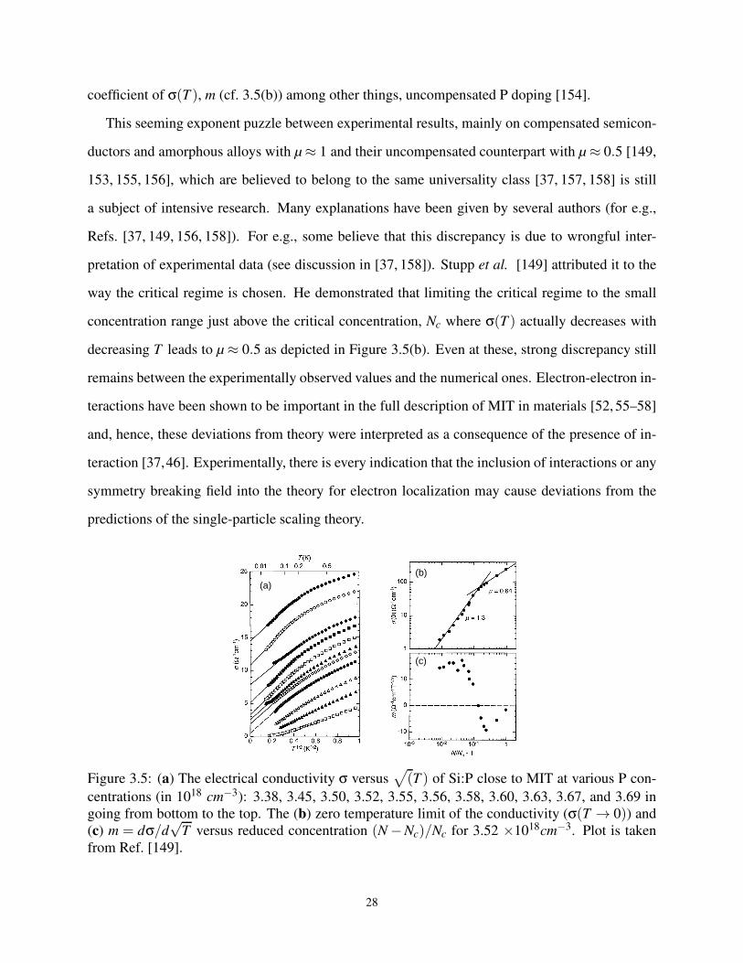
coefficient of σ(T ), m (cf. 3.5(b)) among other things, uncompensated P doping [154].
This seeming exponent puzzle between experimental results, mainly on compensated semicon-
ductors and amorphous alloys with µ ≈ 1 and their uncompensated counterpart with µ ≈ 0.5 [149,
153, 155, 156], which are believed to belong to the same universality class [37, 157, 158] is still
a subject of intensive research. Many explanations have been given by several authors (for e.g.,
Refs. [37, 149, 156, 158]). For e.g., some believe that this discrepancy is due to wrongful inter-
pretation of experimental data (see discussion in [37, 158]). Stupp et al. [149] attributed it to the
way the critical regime is chosen. He demonstrated that limiting the critical regime to the small
concentration range just above the critical concentration, Nc where σ(T ) actually decreases with
decreasing T leads to µ ≈ 0.5 as depicted in Figure 3.5(b). Even at these, strong discrepancy still
remains between the experimentally observed values and the numerical ones. Electron-electron in-
teractions have been shown to be important in the full description of MIT in materials [52, 55–58]
and, hence, these deviations from theory were interpreted as a consequence of the presence of in-
teraction [37,46]. Experimentally, there is every indication that the inclusion of interactions or any
symmetry breaking field into the theory for electron localization may cause deviations from the
predictions of the single-particle scaling theory.
Figure 3.5: (a) The electrical conductivity σ versus√
(T ) of Si:P close to MIT at various P con-
centrations (in 1018 cm−3): 3.38, 3.45, 3.50, 3.52, 3.55, 3.56, 3.58, 3.60, 3.63, 3.67, and 3.69 in
going from bottom to the top. The (b) zero temperature limit of the conductivity (σ(T → 0)) and
(c) m = dσ/d√
T versus reduced concentration (N −Nc)/Nc for 3.52 ×1018cm−3. Plot is taken
from Ref. [149].
28
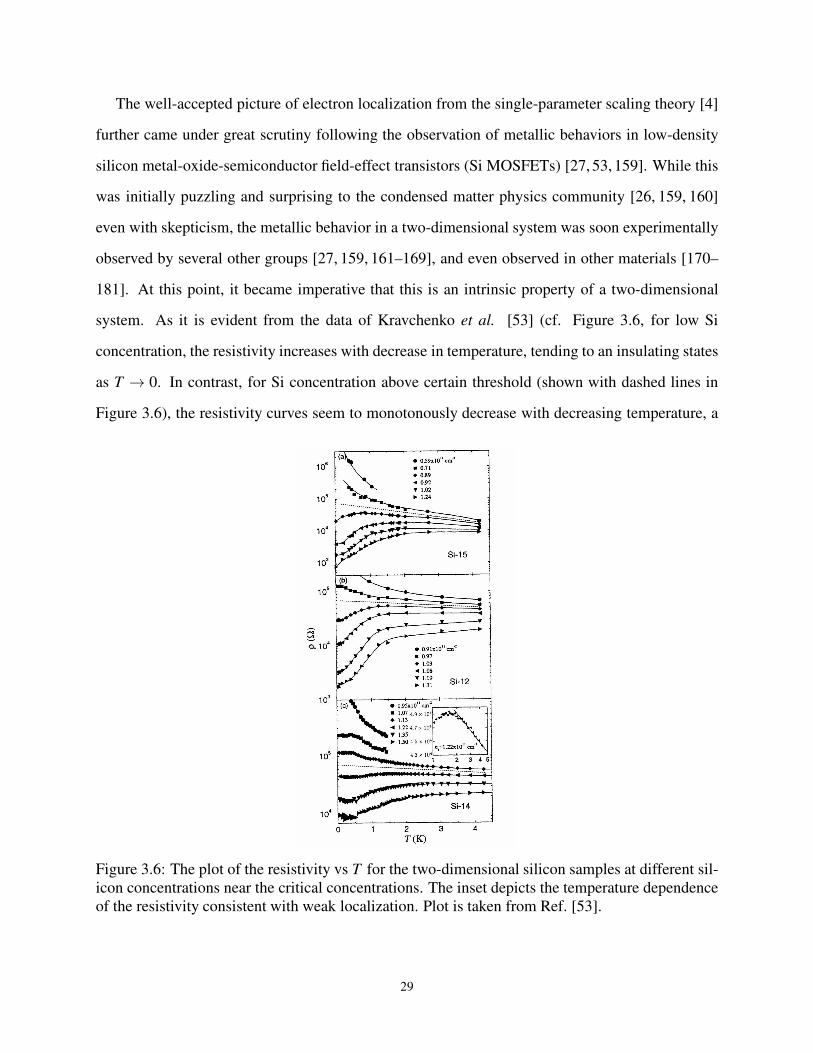
The well-accepted picture of electron localization from the single-parameter scaling theory [4]
further came under great scrutiny following the observation of metallic behaviors in low-density
silicon metal-oxide-semiconductor field-effect transistors (Si MOSFETs) [27, 53, 159]. While this
was initially puzzling and surprising to the condensed matter physics community [26, 159, 160]
even with skepticism, the metallic behavior in a two-dimensional system was soon experimentally
observed by several other groups [27, 159, 161–169], and even observed in other materials [170–
181]. At this point, it became imperative that this is an intrinsic property of a two-dimensional
system. As it is evident from the data of Kravchenko et al. [53] (cf. Figure 3.6, for low Si
concentration, the resistivity increases with decrease in temperature, tending to an insulating states
as T → 0. In contrast, for Si concentration above certain threshold (shown with dashed lines in
Figure 3.6), the resistivity curves seem to monotonously decrease with decreasing temperature, a
Figure 3.6: The plot of the resistivity vs T for the two-dimensional silicon samples at different sil-
icon concentrations near the critical concentrations. The inset depicts the temperature dependence
of the resistivity consistent with weak localization. Plot is taken from Ref. [53].
29
signature of metallic states. This conundrum implies that if the latter case (low Si concentration)
extrapolates to an insulating ground state as T → 0 then, there exists a metal-insulator-transitions
in two-dimensions in violation of the predictions of the single-parameter scaling theory 5. While
this is surprisingly, the 1/N expansion in 2+ ε dimensions by Ma and Fradkin [18] found a new
“interacting” fixed point in their study on localization and interactions in a disordered electron
gas [18].
Over the years, the conjecture and premise of the above observations and interpretation have
been under debate especially from the theoretical point of view since it violates the single-parameter
scaling. Notable among them is the question of the relevant temperature scale used in the ex-
periments since the Fermi temperature of the probes used in the experiments is rather low as a
consequence of the low sample concentrations. Thus, the observed metallic behavior may be
due to finite temperature effects with the insulating states becoming robust at much lower tem-
peratures [26, 176, 182–187]. This is the so-called temperature-dependent screening [188–190].
Temperature dependent disorder scattering [170, 191] and spin-orbit splitting of different spin
subbands [192, 193] have also been proposed to explain this puzzle. Another school of thought
suggests the modification of the single-parameter scaling theory to two-parameter scaling the-
ory, which permits, within a certain parameter regime, for a metallic solution even in two di-
mensions [19, 47, 194, 195]. This line of thought was pursued by Finkel’stein and co-workers,
using renormalization group arguments, to predict the existence of a quantum critical point in two
dimensions (2D) [19], the validity of which was confirmed by experiments in 2D Si-metal-oxide-
semiconductor field-effect transistors [20]. In the weak disorder regime, perturbative simulations
showed that spin and valley degeneracy [47,196] may be important, which in the limit of an infinite
number of valleys, a non-Fermi-liquid metallic state is shown to be stabilized by electron interac-
tions [19,169,181]. The role of electron interactions was also explored and numerical studies have
shown that interactions lead to delocalization in two-dimensions [29, 197–201]. Many other theo-
retical proposals were put forward to explain MIT in 2D. Among them is idea of the admixture of a
Fermi liquid and a Wigner crystal [199,202,203] at the same energy, a variant of the Wigner-Mott
5The possibility of spin-orbit coupling, which breaks time-reversal symmetry can at least be excluded from the experimental data since there is
no applied magnetic field or atom with a strong moment.
30

transition [204, 205]. The role of percolation phenomenon at the MIT [172, 206–209] and local
moments [157, 210] have been investigated, and some argue that the emergence of metallic phase
in 2D may be a signature of a superconducting phase [211–213] Many other viewpoints were also
suggested (see for e.g., [27]), but after many decades of intense research, no generally accepted
theory has been formulated for the theoretical description of electron localization not only in two
dimensions but also in one and three dimensions. Whatever may be the case, experimental results
suggest that for the accurate description of electron localization in materials, a good understand of
the interplay between disorder and electron interactions is very central (see for e.g. [52, 55–58].
This will be the focus of Chapter 10.
To further demonstrate the importance of systematic incorporation of electron-electron interac-
tions to the interpretations of an MIT, Richardella et al. [52] using scanning tunneling microscopy,
visualized the evolution of the local density of states of Ga1−xMnxAs samples at various Mn dop-
ing. The authors demonstrated that a combined effects of strong spatial variation and electron-
electron interactions leads to the suppression of the the tunneling density of states near the Fermi
energy. As shown in Figure 3.7 (A-C), spectroscopic maps of the local density of states at the
Figure 3.7: The spatial variation of the LDoS in the proximity of the Fermi energy at (A)
1.5% Mn doping, Ga0.985Mn0.015As, (B) 3% Mn doping, Ga0.97Mn0.03As, (C) 5% Mn doping,
Ga0.95Mn0.05As. (D) The normalized local distribution of the differential conductance. The inset
is the multifractal spectrum f (α) near the Lipschitz-Hölder exponent, which gives the maximum
of the multifractal spectrum. Plot is taken from Ref. [52].
31
Fermi energy at different dopings depicts varying spatial variation [141]. For extended states, the
distribution of the LDoS are expected to show Gaussian distribution, an indication that the LDoS
have equal weight on every site. However, close to the metal-insulator-transitions, different en-
ergy scales are expected to emerge especially in the LDoS such that a cross-over from a Gaussian
(characteristic of a metal (cf. gray circle in Figure 3.7 (D))) to a log-normal (insulator) behavior
starts to emerge even in the weak localization limit [52, 214, 215], but decreasing the doping leads
to more skewness of the distribution of the LDoS, i.e., log-normal distribution (Figure 3.7 (D)).
The inset of Figure 3.7 (D) shows that even in the presence of electron-electron correlation, the
spectrum remains multifractal as in the non-interacting regime.
32
Chapter 4
Models of Disordered and Interacting
Electronic Systems
Over the years, many models have been proposed and developed for the study of disordered and
interacting systems, and for studying their combined effects. Prominent amongst them are the
Anderson model for disordered electron system [4, 35, 69], which is a tight-binding model for
characterizing a disordered electron system. For the study of interacting system, the Hubbard
model [216–219] has been rigorously used while to study both the effect of interactions and dis-
order at the same time, the Anderson-Hubbard model [69, 220] has been consistently used. While
there are other various models for studying disordered interacting systems (and their combined ef-
fects), in this dissertation, the focus will be on the above mentioned three models. No attempt will
be made to cover all the known facts about these models but an overview just enough to interpret
the present results will be explained.
4.1 Anderson Model of Disordered Electron System
Before delving into the nitty-gritty of the Anderson model of electron localization, a general
overview of the Anderson model will be presented.
Anderson Model: “More is different” [221]; a conjecture pointed out by Anderson [221], when
confronted by a change of scale, the behavior of large and complex system might not always be
a straightforward extrapolation of the well-known simple behavior of its small-scale components.
When increasing the complexity or adding more atoms to a system, its behavior might change
drastically in nature: it may undergo a phase transition. The Anderson model of localization is
the simplest yet a paradigmatic model for describing electronic transport properties of disordered
quantum systems [36, 222]. It has been used successfully used to study amorphous materials such
33
as alloys [223], semiconductors, and even DNA [224]. Its hallmark is the prediction of a spatial
confinement of the electronic motion upon increasing the disorder strength; a phenomenon known
as the Anderson localization transitions [35]. In 3D, a metal-insulator-transition occurs as disorder
strength W mediates a change of transport properties from metallic behavior at small W via critical
behavior at the transition WU=0c to insulating behavior and strong localization at larger W [36,106].
In particular, in the 1958 seminal paper by Anderson [35], he observed that a large piece of
disordered material can become an insulator, even when its elementary blocks have a metallic be-
havior. This phenomenon has come to be known as Anderson localization. Anderson localization
basically results from a subtle interference effect of the backscattered coherent waves propagating
in a random medium [225]. While Anderson’s prediction remained unappreciated and wasn’t fully
recognized by the scientific community for up to a decade, it, however, has led to a new paradigm
in the way we characterize the transport properties of disordered materials. Anderson localiza-
tion in general exhibit universality, which has led to the spread of its application in many other
fields, which is not limited to the following: the study of condensed matter systems [36, 69, 226],
optical and ultra cold atoms [227–233], disordered quantum systems [36, 40], seismic [234, 235],
photonic lattices in the form of matter waves [227, 236], electromagnetic absorption in a disor-
dered medium [86, 237], superfluid helium in porous media [238], molecular and biological sys-
tems [239–241], and even disordered superconductors [46].
The original Anderson model is a simple model for describing the diffusion or conduction of
electrons in the impurity band (disordered system). The Anderson model of disorder has stood
the test of time and provides rather accurate, single-particle description of disordered electronic
systems. The Anderson model for the non-interacting electrons moving on a lattice with a diagonal
on-site random disorder potential is given by the Hamiltonian
H =−t ∑<i, j>
(c†i c j + c
†jci)+∑
i
(Vi −µ)ni. (4.1)
The disordered part is modeled by a local potential Vi, which is a random quantity distributed
according to some specified probability distribution P(Vi). The operators c†i (ci) create (annihilate)
34
a quasiparticle on site i and ni = c†i ci is the number operator, µ is the chemical potential, and t is the
hopping matrix element between nearest-neighbor < i, j >. We set 4t = 1 as the energy unit. In our
analysis, we use different types of disorder distributions. In particular, we consider the box (Bo),
Gaussian (Ga), Lorentzian (Lo), and binary (Bi) distributions, respectively, with the distribution
functions P(Vi)
PBo(Vi) =1
2WBoΘ(WBo −|Vi|), (4.2a)
PGa(Vi) =
√
6
πW 2Ga
e−6V 2i /W 2
Ga , (4.2b)
PLo(Vi) =WLo
π(V 2i +W 2
Lo), (4.2c)
PBi(Vi) = caδ(Vi −WA)+ cbδ(Vi −WB). (4.2d)
where Θ(x) is a step function, ca is the concentration of the host A atom, cb = 1− ca is the
concentration of the impurity B atom, and the strength of the disorder in units of 4t is parameterized
by W (WA and WB for binary alloy model). We have scaled the WGa such that the second moments
of the PBo and PGa agree with each other (i.e., we set the variance of the Gaussian distribution equal
to that of the box distribution: σ2 = W 2/12) in the event that WBo=WGa to enable comparison.
Since the Lorentzian distribution lacks second moment, the disorder values cannot be directly
compared with that of either the box or Gaussian distributions, respectively. We introduce short-
hand notation for disorder averaging 〈...〉=∫
dViP(Vi)(...).
The Anderson model of a disorder is characterized by two energy scales, t and Vi. For the
dimensionless ratio W/t larger than some critical value (W/t)c, all states are said to be localized
while below this critical value, there is a mobility edge (cf. Figure 3.2) with the consequence that
all states are extended [242].
The Anderson localization transition (ALT) [4, 35] is one of the oldest problem in a disordered
electronic system. Already, there have been diverse theoretical studies employing computational
techniques of varying complexity not limited to the numerical exact methods (including the exact
diagonalization, transfer matrix, and kernel polynomial methods), [106, 132, 243–251] varying
35
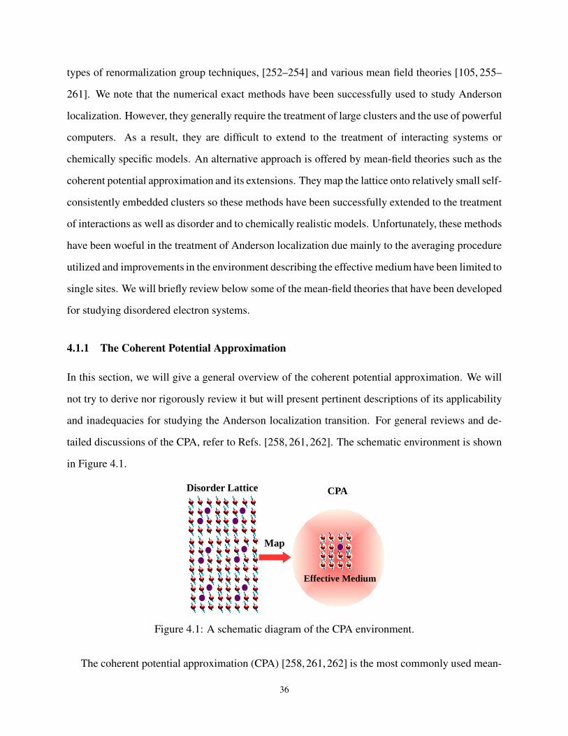
types of renormalization group techniques, [252–254] and various mean field theories [105, 255–
261]. We note that the numerical exact methods have been successfully used to study Anderson
localization. However, they generally require the treatment of large clusters and the use of powerful
computers. As a result, they are difficult to extend to the treatment of interacting systems or
chemically specific models. An alternative approach is offered by mean-field theories such as the
coherent potential approximation and its extensions. They map the lattice onto relatively small self-
consistently embedded clusters so these methods have been successfully extended to the treatment
of interactions as well as disorder and to chemically realistic models. Unfortunately, these methods
have been woeful in the treatment of Anderson localization due mainly to the averaging procedure
utilized and improvements in the environment describing the effective medium have been limited to
single sites. We will briefly review below some of the mean-field theories that have been developed
for studying disordered electron systems.
4.1.1 The Coherent Potential Approximation
In this section, we will give a general overview of the coherent potential approximation. We will
not try to derive nor rigorously review it but will present pertinent descriptions of its applicability
and inadequacies for studying the Anderson localization transition. For general reviews and de-
tailed discussions of the CPA, refer to Refs. [258, 261, 262]. The schematic environment is shown
in Figure 4.1.
Figure 4.1: A schematic diagram of the CPA environment.
The coherent potential approximation (CPA) [258,261,262] is the most commonly used mean-
36
field theory to study disordered electronic systems. In the CPA implementation, the original infinite
disordered lattice is mapped onto an averaged single (momentum-independent) impurity embed-
ded in an effective medium (cf. Fig 4.1). It has been successful in describing some one-particle
properties such as the density of states in (substitutional) disordered alloys [258, 261]. However,
it has failed to provide adequate physics describing Anderson localization transition (ALT). This
failure stems from the local nature of the CPA, as such, it is unable to capture crucial multiple
backscattering interference effects that lead to localization and also on the averaging procedure in
the self-consistency [2, 36].
4.1.2 Cluster Extensions of Coherent Potential Approximation
Over the years, several efforts have been made to extend the CPA to cluster forms to accommodate
spatial corrections that are missing. A typical example of these cluster extensions of the CPA is
the dynamical cluster approximation (DCA) [263, 264] and the molecular CPA (MCPA) [265].
We note the problems encountered in early attempts to formulate cluster corrections to the
dynamical mean-field approximation are the same as those encountered in the coherent potential
approximation (CPA) for disordered systems. As extensively demonstrated by Gonis [266, 267], a
successful quantum cluster theory must meet the following criteria
• A successful quantum cluster theory for a disordered system must be able to self-consistently
and systematically account for the local fluctuations in the effective environment;
• In the limit of the cluster size being one (Nc → 1), it must recover the CPA;
• In the limit of large cluster size (Nc → ∞, the thermodynamic limit), it must become exact;
• It should be numerically tractable and easy to implement;
• A successful cluster theory must obey translational invariance and preserve the full point-
group symmetry of the lattice;
• It should be fully causal so that the self-energy and the associate Green function is analytic in
the upper half-plane.
37
The dynamical cluster approximation has been shown to obey all the above outlined properties
of a successful quantum cluster [263, 264, 267]. So far, it remains one of the most successful
cluster extension of the CPA. The DCA, unlike the CPA, maps a disordered, infinite lattice to a
finite cluster size Nc self-consistently embedded in the effective medium. We will not give detailed
explanation of the self-consistent formalism of the DCA until later where we will describe it in our
implementation of the DCA-based method for studying the Anderson localization transition.
We remark that, even though, spatial correlations are included in these cluster extensions of the
CPA, none of them is adequate for studying Anderson localization transition. The main problem
with these methods is that they use algebraic averaging (in the density of states (DoS)) in their
self-consistency. The average DoS calculated within such mean-field theories cannot distinguish
between extended and localized states and it is not critical at the transition [1, 2, 70, 120]. Hence,
such average quantities cannot be used as an order parameter. This is the reason that most mean-
field theories like the CPA [262] and its cluster extensions including the DCA [263, 264, 267],
fail to provide a proper description of Anderson localization in disordered systems. This failure
is intrinsic to these theories as the algebraically averaged quantities, i.e., the averaged density
of states, used always favor the metallic state. This can be understood from the fact that in an
infinite system of localized states, the average density of states is nothing but the global density
of states, which is a smooth function of the disorder strength near the critical point while the
local density of states becomes discrete with a non-trivial system size dependence (See for e.g.,
Refs. [65, 70, 105, 120, 134, 138, 225, 268] for a detailed discussion). I will demonstrate later
the failures of finite cluster extensions of the CPA in characterizing the Anderson localization
transitions using the DCA.
4.1.3 Algebraic versus Typical Averaging Procedure
Finding a proper single-particle order parameter for the Anderson localization transitions capable
of distinguishing between the localized and extended states is a major challenge in the study of
disordered electronic systems. The study of disordered systems relies on probability distribution
functions (PDFs) to measure ‘random’ quantities of interest. To characterize localization, the most
38
important quantity in the majority of physical or statistical problems is usually the “typical” value
of the ‘random’ variable, which corresponds to the most probable value of the PDF [136]. In most
systems the nature of the PDF is not known a priori; as such, we have limited information via
the moments or cumulants of the PDFs. Under such situation, the “typical” or the most probable
value of the PDF [136] contains important and direct information. Different from some systems
where the first moment (the arithmetic average) is a good estimate of the random variable, the
Anderson localization is a non-self-averaging phenomenon. Close to the critical point the elec-
tronic quantities fluctuate strongly and the corresponding PDF of the local density of states is very
asymmetric with long tails [135, 138] such that infinitely many moments are needed to describe
it [136]. In some cases, the corresponding moments might not even exist especially close to the
critical point [139].
The arithmetic average of random one-particle quantities is not critical at the Anderson local-
ization transition. In contrast to the arithmetic average, the geometrical average, [65,105,135,138,
269] gives a better approximation to the most probable value of the local density of states.
4.1.4 The Typical Medium Theory
As explained in Sections 4.1.1 and 4.1.2, the failures of CPA and its cluster extensions to properly
characterize the localization transitions stem from the utilization of the algebraic average density
of state (DoS) in their self-consistency loop. The average DoS does not vanish at the Anderson
localization transition (ALT) as such, not critical [70]. However, the geometrical mean of the local
DoS (LDoS) [60, 65, 269], which better approximates the typical value of the LDoS is critical at
the ALT.
Dobrosavljevic et al. [105] incorporated the typical medium theory (TMT) to the study of
disorder system, where the typical density of states (TDoS) approximated using the geometrical
averaging over disorder configurations are used instead of the arithmetically averaged local density
of states. They demonstrated that the TDOS vanishes continuously as the strength of the disorder
increases towards the critical point, and it can be used as an effective mean-field order parameter for
the Anderson localization. In principle, Dobrosavljevic et al. [105] showed that the typical density
39
of states (TDOS) provides a single-particle local order parameter for describing the Anderson
localization transitions.
While the single-site TMT has been shown to be successful in describing localized electron
states, it still has several drawbacks. In particular, it does not provide a proper description of the
critical behavior of the Anderson localization transitions in 3-dimensions (3D). The local TMT un-
derestimates the critical disorder strength with W T MTc = 1.65 instead of the numerical exact value
Wc ≈ 2.1 [37, 131, 247, 270–274] for the box distribution (in the units of our computations). Also,
the universal order parameter critical exponent, (which has also been called the typical order pa-
rameter exponent) [135] β obtained in the local TMT is βTMT ≈ 1.0 whereas the recently reported
value is β ≈ 1.67 [142,271]. Another crucial drawback of the single site TMT in three-dimensions
is its inability to capture the re-entrance behavior of the mobility edge (energy separating extended
and localized electron states) (for the disorder distributions with finite variance e.g., the box, and
Gaussian disorder distributions) as seen in exact numerical studies [242, 272, 275]. The TMT also
underestimates the extended region in all the disorder distributions studied in this dissertation.
The inadequacies of the local TMT can be remedied by incorporating spatial (non-local) corre-
lations via its cluster extension. This can be achieved by using the DCA schemes, which systemat-
ically incorporates the missing non-local effects. This is another task of this dissertation and I will
show that a straightforward extension of the local TMT is not just enough as it suffers from clus-
ter self-averaging, which destroys the localization transitions. To avoid such self-averaging issues
in the TDoS, a different Typical Medium DCA (TMDCA) method is proposed, which explicitly
separates out the local part of the TDoS and treating it with a geometric averaging over disorder
configurations. In this way, a proper TDoS that characterizes the ALT in 3D is obtained.
4.2 Hubbard Model
The Hubbard model is the simplest yet versatile model of interacting particles in a lattice. The
original formulation of the Hubbard model was to describe electrons in solids [216] but it has
since been the center of interest as a model for the high-temperature superconductivity, ultracold
40
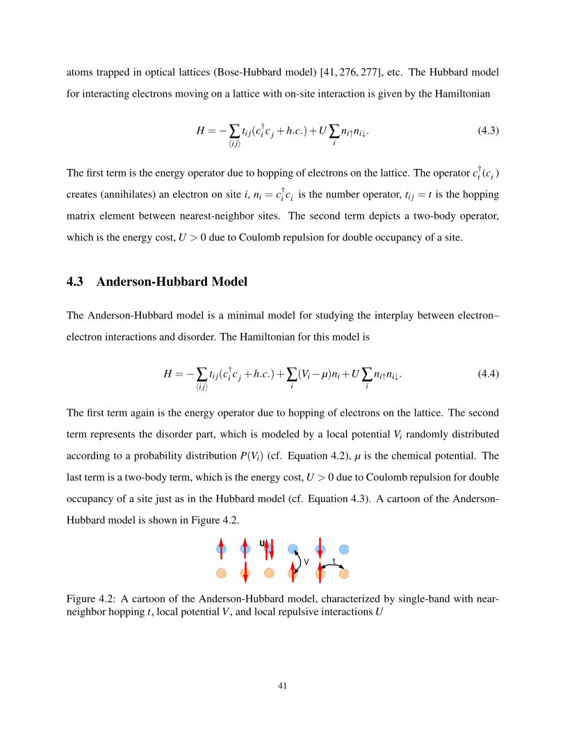
atoms trapped in optical lattices (Bose-Hubbard model) [41, 276, 277], etc. The Hubbard model
for interacting electrons moving on a lattice with on-site interaction is given by the Hamiltonian
H =−∑〈i j〉
ti j(c†i c j +h.c.)+U ∑
i
ni↑ni↓. (4.3)
The first term is the energy operator due to hopping of electrons on the lattice. The operator c†i (ci )
creates (annihilates) an electron on site i, ni = c†i ci is the number operator, ti j = t is the hopping
matrix element between nearest-neighbor sites. The second term depicts a two-body operator,
which is the energy cost, U > 0 due to Coulomb repulsion for double occupancy of a site.
4.3 Anderson-Hubbard Model
The Anderson-Hubbard model is a minimal model for studying the interplay between electron–
electron interactions and disorder. The Hamiltonian for this model is
H =−∑〈i j〉
ti j(c†i c j +h.c.)+∑
i
(Vi −µ)ni +U ∑i
ni↑ni↓. (4.4)
The first term again is the energy operator due to hopping of electrons on the lattice. The second
term represents the disorder part, which is modeled by a local potential Vi randomly distributed
according to a probability distribution P(Vi) (cf. Equation 4.2), µ is the chemical potential. The
last term is a two-body term, which is the energy cost, U > 0 due to Coulomb repulsion for double
occupancy of a site just as in the Hubbard model (cf. Equation 4.3). A cartoon of the Anderson-
Hubbard model is shown in Figure 4.2.
Figure 4.2: A cartoon of the Anderson-Hubbard model, characterized by single-band with near-
neighbor hopping t, local potential V , and local repulsive interactions U
41
Chapter 5
Typical Medium Dynamical Cluster
Approximation
In this Chapter, pedagogical steps in formulating a systematic, self-consistent finite cluster mean-
field theory for ‘proper’ characterization of electron localization will be presented.
5.1 Introduction
Decades of efforts to formulate a systematic, self-consistent theory capable of properly charac-
terizing the localization transitions in electronic systems have not been overwhelmingly achieved.
Aside the single site TMT [105], other variants of the mean-field theories formulated to describe
the localization transition have not been successful. However, as explained above, the local TMT
has several drawbacks. Among them is the underestimation of the critical disorder strength, order
parameter critical exponent, the inability to capture the re-entrance of the mobility edge (in dis-
tributions with finite variance), and the underestimation of the extended states in all the disorder
distributions explored in this dissertation. One can thus conclude that, even though, the single site
TMT gives a qualitative description of the localization transitions, it however fails to describe it
quantitatively.
As a consequence of the central importance of an effective mean-field method (that properly
describes the Anderson localization transition) to further progress in the study of electron local-
ization, there is a need to formulate a mean-field theory that properly characterizes (both quanti-
tatively and qualitatively) the localization transitions. Furthermore, a well-known long historical
dichotomy exists between the mean-field results and the numerical data for the localization transi-
tion. Here, we demonstrate that the dichotomy can be reconciled by incorporating spatial fluctua-
tions (in a typical environment) into the mean-field theory offering a solution to this long-standing
42

problem, by providing a systematic framework in the mean-field theory of Anderson localization
including the off-diagonal disorder and interactions.
5.2 Formulation of Typical Medium Dynamical Cluster Approximation
The typical medium dynamical cluster approximation (TMDCA) utilizes the self-consistent frame-
work of the standard dynamical cluster approximation [264, 278] with the important usage of an
environment defined by a typical non-local hybridization function Γ(K,ω) (cf. Fig 5.1(a)). In par-
ticular, the TMDCA maps the given disordered lattice system into a finite periodic cluster of size
Nc = Ldc which is embedded in an effective self-consistent typical medium (c.f. Figure 5.1(a)).
Note that unlike in the usual DCA scheme where the effective medium is constructed via al-
gebraic averaging over disorder configurations, in the TMDCA scheme, geometric averaging is
used. By mapping a d-dimensional lattice containing N sites to a finite small cluster containing
Nc = Ldc sites, where Lc is the linear dimension of the cluster, we dramatically reduce the com-
putation effort [267]. The mapping is accomplished by dividing the first Brillouin zone into Nc
non-overlapping cells of equal size (cf. Fig 5.2(a)). We show in Fig 5.2(b) how the coarse-graining
procedure is achieved for a cluster of size Nc = 4 in 2-dimensions while Fig 5.2(c) depicts the tiling
procedure for some clusters.
Unlike the single-site methods commonly used to study disordered systems, such as the coher-
ent potential approximation (CPA) [258, 262] or the local TMT, [105] the TMDCA ensures that
non-local, spatial fluctuations, which are neglected in single-site approaches, are systematically
incorporated as the cluster size Nc increases. Short length scale correlations inside the cluster are
treated exactly up to a range ξ . Lc, while the long length scale correlations are treated within the
typical medium (cf. Figure 5.1(a)). At the limit of cluster size Nc = 1, the TMDCA recovers the
local TMT, and at the limit of Nc → ∞, the TMDCA becomes exact. Hence, between these two
limits, the TMDCA systematically incorporates non-local correlations into the local TMT.
One of hardest task in developing a (cluster) formalism for characterizing the localization is
among other things, the solution to remain causal, fulfill all the essential requirements expected
43
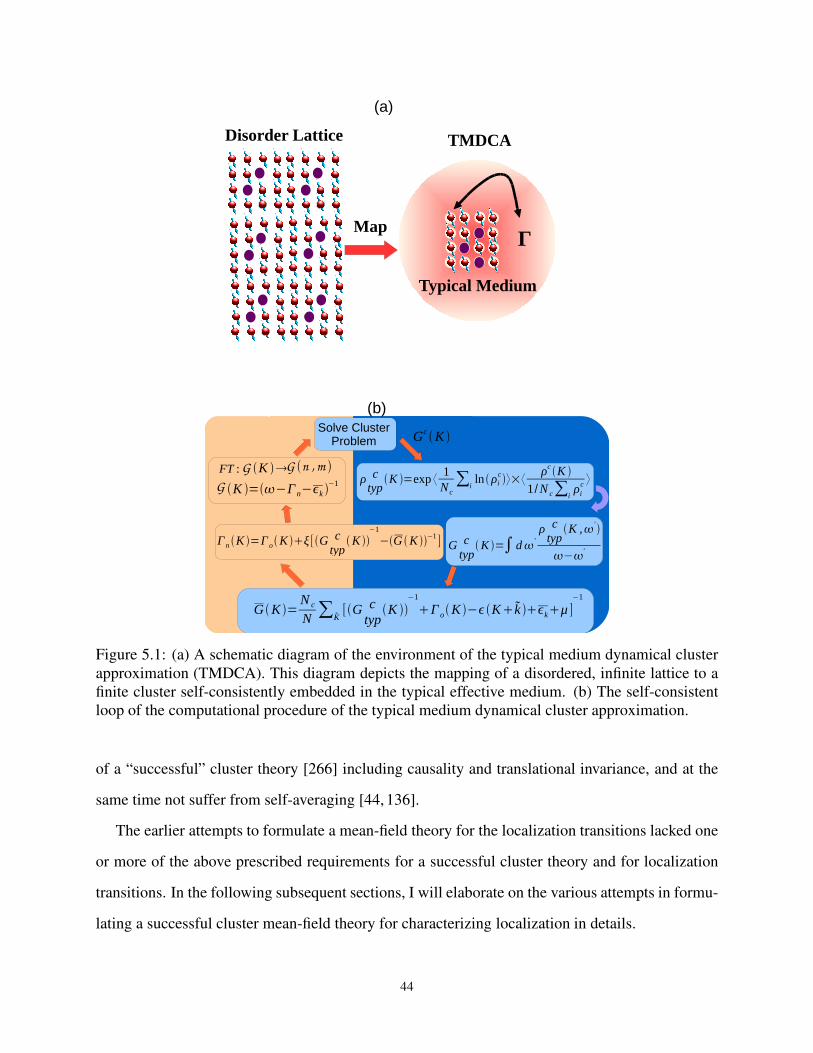
Figure 5.1: (a) A schematic diagram of the environment of the typical medium dynamical cluster
approximation (TMDCA). This diagram depicts the mapping of a disordered, infinite lattice to a
finite cluster self-consistently embedded in the typical effective medium. (b) The self-consistent
loop of the computational procedure of the typical medium dynamical cluster approximation.
of a “successful” cluster theory [266] including causality and translational invariance, and at the
same time not suffer from self-averaging [44, 136].
The earlier attempts to formulate a mean-field theory for the localization transitions lacked one
or more of the above prescribed requirements for a successful cluster theory and for localization
transitions. In the following subsequent sections, I will elaborate on the various attempts in formu-
lating a successful cluster mean-field theory for characterizing localization in details.
44
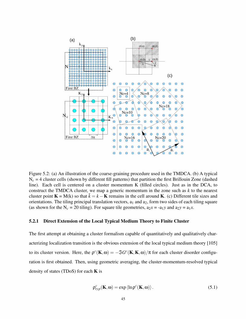
Figure 5.2: (a) An illustration of the coarse-graining procedure used in the TMDCA. (b) A typical
Nc = 4 cluster cells (shown by different fill patterns) that partition the first Brillouin Zone (dashed
line). Each cell is centered on a cluster momentum K (filled circles). Just as in the DCA, to
construct the TMDCA cluster, we map a generic momentum in the zone such as k to the nearest
cluster point K = M(k) so that k = k−K remains in the cell around K. (c) Different tile sizes and
orientations. The tiling principal translation vectors, a1 and a2, form two sides of each tiling square
(as shown for the Nc = 20 tiling). For square tile geometries, a2x = -a1y and a2y = a1x.
5.2.1 Direct Extension of the Local Typical Medium Theory to Finite Cluster
The first attempt at obtaining a cluster formalism capable of quantitatively and qualitatively char-
acterizing localization transition is the obvious extension of the local typical medium theory [105]
to its cluster version. Here, the ρc(K,ω) = −ℑGc(K,K,ω)/π for each cluster disorder configu-
ration is first obtained. Then, using geometric averaging, the cluster-momentum-resolved typical
density of states (TDoS) for each K is
ρctyp(K,ω) = exp〈lnρc(K,ω)〉 . (5.1)
45
As will be elaborated in details in Subsection 5.3.1, defining the typical density of states as in
Equation 5.1 suffers from cluster self-averaging as Nc → ∞ in three dimensions. However, it does
reproduce the expected behavior in lower (one and two) dimensions as will be shown in Chapter 6.
Further, the inability of the direct extension of the local typical medium theory to finite cluster
to fully capture the localization transitions in three dimensions can be inferred from Figure 5.3.
While it will eventually converge, it will converge to a critical disorder strength far greater than the
numerically known value. A further remark is that the trajectories of the mobility edge is totally
missed due to self-averaging. I will elaborate on this later in Subsection 5.3.1.
Another version of the initial attempt to develop cluster theory for the localization transition is
the separation of the local densities (typical and algebraic) in such a way that a fraction of their
ratio multiples the local typical density while the remaining fraction multiples the algebraic cluster
density of states as
ρctyp(K,ω) =
1.0−exp(
1Nc
∑Nc
i=1 〈lnρci (ω,V )〉
)
1Nc
∑Nc
i=1
⟨ρc
i (ω,V )⟩
× exp
(
1
Nc
Nc
∑i=1
〈lnρci (ω,V )〉
)
+
exp(
1Nc
∑Nc
i=1 〈lnρci (ω,V )〉
)
1Nc
∑Nc
i=1
⟨ρc
i (ω,V )⟩
×〈ρc(K,ω,V )〉
. (5.2)
This again does reproduce the expected behavior in lower dimensions but not in three dimensions
due to the same reasons as explained above, it is possible to formulate variants of other definitions
of the typical medium, which avoid self-averaging. One of the possibility is just utilizing the local
part of the typical density of states as
ρctyp(K,ω) = exp
(
1
Nc
Nc
∑i=1
〈lnρci (ω,Vi)〉
)
. (5.3)
However, while this formulation avoids self-averaging as Nc → ∞, it does not meet some of the
criteria of a successful cluster theory. In particular, this formalism does not recover the DCA in
the weak coupling limit. This will be demonstrated below. It should be noted that while the first
two formulations (cf. Eqs. 5.1 and 5.2), meets all the requirements needed of a successful cluster
46
theory, it does suffer from cluster self-averaging as Nc → ∞. For all the formulations above, to
ensure the causality of the Green function, we carry out the Hilbert transformation of the TDoS to
obtain the typical cluster Green function as
Gctyp(K,ω) =
∫dω′ρ
ctyp(K,ω′)
ω−ω′ . (5.4)
5.3 The Typical Medium Dynamical Cluster Approximation
After several attempts and formulating variants of the finite cluster theory for localization transi-
tions, the typical medium dynamical cluster approximation (TMDCA) was developed. The typical
medium dynamical cluster approximation scheme is, to the best of my knowledge, a successful,
systematic, self-consistent, preserving causality, and numerically efficient effective medium the-
ory to characterizing localization transitions in one, two, and three dimensions. For instance, in the
Anderson localization transitions where broad transition exists in three-dimensions, the TMDCA,
i) recovers the original single-site TMT scheme at cluster size Nc = 1; ii) recovers the DCA results
at small disorder strength (when all states are metallic); iii) provides a proper way to separate the
energy scales such that the characteristic mobility edge behavior (for the disorder distributions with
finite variance) is obtained; iv) captures the critical behavior of Anderson localization transitions
with correct critical disorder strength Wc and order parameter critical exponent β, and provides a
correct description of the Anderson insulator at large disorder strength (when all states are local-
ized); v) fulfills all the essential requirements expected of a “successful” cluster theory [264,266].
Before presenting detailed self-consistent algorithm of the TMDCA, an explanation of the ori-
gin of the cluster self-averaging in the earlier attempts to develop a cluster version of the typical
medium theory will be discussed.
5.3.1 Avoiding Self-Averaging
As it is obvious from above, the averaging procedure used to calculate the typical spectra is not
unique. As noted above, a direct extension of the local typical medium theory (TMT) [105] to
finite cluster reproduced the expected behavior in one and two dimensions as Nc is increased [1].
47
However, in three dimension, applying the algorithm directly will lead to effective self-averaging
for large clusters. This is due to the fact that close to the criticality, there exist distinct localized
and extended states above and below the localization edge given by the TDoS with an energy scale
difference that can span an order of magnitude. These energy scales need to be treated differently.
This can be seen by investigating the spectra density where the local part of the TDoS is not
explicitly separated and treated with geometric averaging over disorder realizations:
ρctyp(K,ω) = exp〈lnρc(K,ω,Vi)〉 . (5.5)
In forming the Fourier transform
ρc(K,ω,Vi) = ∑X ,X ′
exp(iK · (X −X ′))ρc(X ,X ′,ω,Vi) (5.6)
the average over the cluster coordinates X and X ′, including the local part, X = X ′. I.e., the local
DoS is first summed over the cluster sites and then Fourier transformed to form the local part of
ρc(K,ω). Hence for large clusters, this reduces to linear averaging of the local part instead of
geometrical averaging. As a consequence, the host Green function constructed from ρctyp(K,ω) is
unaware of the TDoS and thus, it is unable to distinguish between the energies above and below
the localization edge.
To avoid such self-averaging in the TDoS, the cluster-momentum-resolved typical density of
states (TDoS) for each K is split into the local and non-local parts. The local part is treated with
geometrical averaging over disorder configurations, while the non-local part is treated either with
an algebraic (referred to as linear-log procedure) or geometric averaging (referred to as log-log
procedure over the disorder configuration. In the linear-log procedure, the local part is treated
with a geometrical averaging while the non-local part is approximated algebraically using linear
averaging as
ρctyp(K,ω) = exp
(
1
Nc
Nc
∑i=1
〈lnρci (ω,Vi)〉
)
×⟨
ρc(K,ω,Vi)1
Nc∑i ρc
i (ω,Vi)
⟩
. (5.7)
48
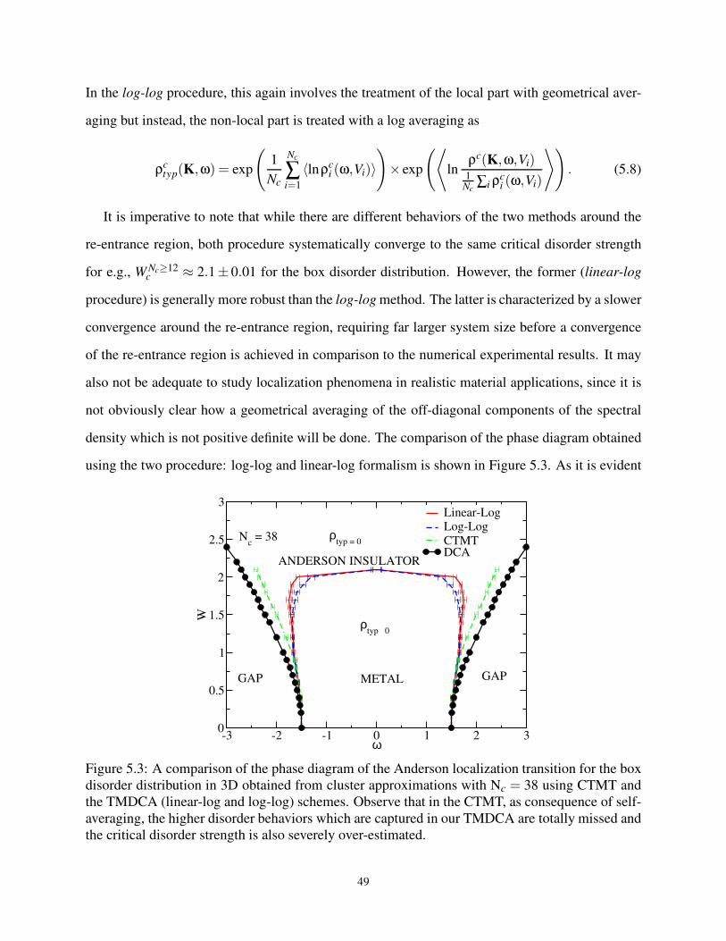
In the log-log procedure, this again involves the treatment of the local part with geometrical aver-
aging but instead, the non-local part is treated with a log averaging as
ρctyp(K,ω) = exp
(
1
Nc
Nc
∑i=1
〈lnρci (ω,Vi)〉
)
× exp
(⟨
lnρc(K,ω,Vi)
1Nc
∑i ρci (ω,Vi)
⟩)
. (5.8)
It is imperative to note that while there are different behaviors of the two methods around the
re-entrance region, both procedure systematically converge to the same critical disorder strength
for e.g., W Nc≥12c ≈ 2.1± 0.01 for the box disorder distribution. However, the former (linear-log
procedure) is generally more robust than the log-log method. The latter is characterized by a slower
convergence around the re-entrance region, requiring far larger system size before a convergence
of the re-entrance region is achieved in comparison to the numerical experimental results. It may
also not be adequate to study localization phenomena in realistic material applications, since it is
not obviously clear how a geometrical averaging of the off-diagonal components of the spectral
density which is not positive definite will be done. The comparison of the phase diagram obtained
using the two procedure: log-log and linear-log formalism is shown in Figure 5.3. As it is evident
-3 -2 -1 0 1 2 3ω
0
0.5
1
1.5
2
2.5
3
W
Linear-LogLog-Log
CTMTDCA
GAP METAL
ρtyp > 0
ANDERSON INSULATOR
GAP
Nc = 38 ρ
typ = 0
Figure 5.3: A comparison of the phase diagram of the Anderson localization transition for the box
disorder distribution in 3D obtained from cluster approximations with Nc = 38 using CTMT and
the TMDCA (linear-log and log-log) schemes. Observe that in the CTMT, as consequence of self-
averaging, the higher disorder behaviors which are captured in our TMDCA are totally missed and
the critical disorder strength is also severely over-estimated.
49
from Fig 5.3, the two new schemes converge to the same critical disorder strength but behave
differently around the re-entrance region. For the results presented in the subsequent Chapters of
this dissertation, the linear-log method is utilized.
Note further that in both the linear-log and log-log procedures, at small Nc, ≈ 100 self-consistent
iterations are required to achieve a convergence while for relatively large Nc, far fewer iterations
are required. The convergence criterion for both limits is achieved when the TDoS (ω = 0) does
not fluctuate anymore with iteration number within the error bars.
5.3.2 Typical Medium Dynamical Cluster Approximation: The Self-Consistent
The details of the formalism of the typical medium dynamical cluster approximation are described
below. The average density of states at each cluster momentum K within the dynamical cluster
approximation is given as
ρcavg(K,ω) = 〈ρc(K,ω)〉=−1
π〈ℑGc(K,K,ω)〉, (5.9)
where the superscript ‘c’ denotes cluster and 〈〉 is the disorder average. The K-dependent cluster
Green function is obtained from the site dependent Green function Gc(i, j,ω) via
Gc(K,K,ω) =1
Nc∑i, j
eiK·(Ri−R j)Gc(i, j,ω). (5.10)
In the TMDCA, for each cluster configuration, ρc(K,ω)= −ℑGc(K,K,ω)/π is first obtained
and can be shown via the Lehmann representation [279,280], that ρc(K,ω)≥ 0 for each K, ω, and
disorder configuration. As explained above, the formulation of the TMDCA utilized in this disser-
tation is the log-linear procedure. Here, the local part of the cluster-momentum-resolved typical
density of states is separated and treat with geometrical averaging over the cluster and disorder
configurations, as to avoid self-averaging as the cluster size increases. The obtained cluster TDoS
50
is given by
ρctyp(K,ω) =
local TDOS
︷ ︸︸ ︷
exp
(
1
Nc
Nc
∑i=1
〈lnρci (ω,V )〉
)
×⟨
ρc(K,ω,V)1
Nc∑i ρc
i (ω,V )
⟩
︸ ︷︷ ︸
non-local
. (5.11)
The ρctyp(K,ω) possess the following properties: for Nc = 1, it reduces to the local TMT scheme
with ρctyp(ω) = exp〈lnρ(ω)〉. At low disorder strength, W ≪Wc, we find the real space prefactor
〈lnρi(ω,Vi)〉 ≈ ln〈ρi(ω,Vi)〉. Then ρctyp(K,ω) reduces to the DoS calculated in DCA scheme,
with ρctyp(K,ω)≈ 〈ρc(K,ω,V)〉 . From Equation 5.11, the disorder averaged typical cluster Green
function is obtained using the Hilbert transform
Gctyp(K,ω) =
∫dω′ρ
ctyp(K,ω′)
ω−ω′ . (5.12)
A schematic one-dimensional TMDCA self-consistency is shown in Figure 5.1(b). The TMDCA
iterative procedure is described:
1. The TMDCA iterative procedure begins by one proposing an initial guess for the hybridiza-
tion function Γo(K,ω), where the subscript o denotes old. The choice of the starting guess
for the hybridization function may be based on a priori knowledge, i.e., in case we have in-
formation about the self-energy Σ(K,ω) and cluster Green function Gc(K,ω), Γo(K,ω) can
be calculated as
Γo(K,ω) = ω− ε(K)+µ−Σ(K,ω)−1/Gc(K,ω) (5.13)
where ε(K) =Nc
N∑k
ε(K+ k) is the coarse-grained bare dispersion with k summed over N/Nc
momenta inside the cell centered at the cluster momentum K [263] (cf. Figure 5.2(b)). How-
ever, if nothing is known a priori, the guess Γo(K,ω)≡ 0 may serve as the starting point.
2. After setting up the cluster problem, the cluster-excluded Green function G(K,ω) is then
calculated as
G(K,ω) = (ω−Γo(K,ω)− ε(K)+µ)−1. (5.14)
Since the cluster problem is solved in real space, I then Fourier transform G(K,ω) to obtain
51

Gn,m = ∑K G(K)exp(iK · (rn− rm)).
3. Next, the cluster problem is solved exactly. Here, I stochastically generate random configura-
tions of the disorder potential V . For each disordered configuration, I use the Dyson equation
to calculate the new fully disorder dressed cluster Green function
Gc(V ) = (G−1 −V )−1. (5.15)
This is Fourier transformed to Gc(K,K,ω) to obtain the cluster density of states ρc(K,ω) =
− 1πℑGc(K,K,ω). The typical cluster density of states is then calculated via geometric aver-
aging using Equation 5.11. Then, we calculate the disorder averaged, typical cluster Green
function Gctyp(K,ω) via Hilbert transform using Equation 5.12. Note the advantage of the
stochastic sampling of the disorder configurations. Here, each of the disorder configurations
is statistically independent of each other. Thus, instead of sampling the disorder configu-
rations with the very expensive enumeration technique which scales as 2Nc, we instead do
a stochastic sampling of the disorder configurations. This greatly reduces the computational
cost enabling us to study larger clusters. With this, the number of disorder realizations needed
to get a converged solution falls with increased cluster size. Furthermore, since fewer itera-
tions are needed for larger clusters the computational cost does not even scale as N3c as one
would expect from Equation 5.15. For a typical 64 site cluster, with box disorder about 500
disorder realizations are enough to produce high-quality data.
4. After solving the cluster problem, I use the typical cluster Green function Gctyp(K,ω), to
calculate the coarse-grained cluster Green function of the lattice G(K,ω) as
G(K,ω) =
∫Nc
0(K,ε)dε
(Gctyp(K,ω))−1+Γ(K,ω)− εK+ ε(K)
, (5.16)
where Nc0(K,ε) is the bare partial density of states.
5. The self-consistency is closed by updating the new hybridization function using linear mixing
Γn(K,ω) = Γo(K,ω)+ξ[(Gctyp(K,ω))−1− (G(K,ω))−1] (5.17)
52
where the subscripts n and o denote new and old, respectively. The mixing parameter ξ > 0
controls the ratio of the new and old Γ(K,ω) entering the next iteration. For very small ξ,
convergence may be slowed down unnecessarily, while for very large ξ, oscillations about the
self-consistent solution may occur. Instead of linear mixing, the convergence of the compu-
tations can be improved by using the Broyden method [281].
6. The above procedure is repeated until the hybridization function converges to the desired
accuracy, Γo(K,ω) = Γn(K,ω). When this happens, the Green functions are also converged,
G(K,ω) = Gctyp(K,ω) within the computational error.
Note the TMDCA just as in the DCA [264, 278] preserves causality. since all the Green func-
tions are causal, both the DoS and the TDoS calculated from them are positive definite. Also, I
observe that as Nc increases, the method systematically interpolates between the local TMT and
the exact result.
5.3.3 The Pole Procedure
Close to the criticality, the states at the top and bottom (for e.g., a bipartite lattice (0,0,0) and
(π,π,π)) of the bands are such that their hybridization rates tend to zero leading to the development
of poles in the cluster excluded Green function. Here, I present in detail how to deal with such
poles that emerge on the real frequency axis as the critical disorder strength is approached.
When ℑΓtyp(K,ω) becomes very small (→ 0), the imaginary part of the cluster-excluded Green
function, G(K,ω), becomes series of a delta function. To see this clearly, we note that
G(K,ω) = (ω−Γtyp(K,ω)− ε(K))−1 =⇒ P (ω−ω′)−1 − iπδ(ω−ω′), (5.18)
where ω′ = ε(K) + ℜΓtyp(K,ω) and “P ” denotes the principle value. Evidently from Equa-
tion 5.18, the poles cannot be represented in the conventional way as a list of frequencies on
the computer with a finite frequency resolution dω. Such difficulty can be avoided by explicitly
53
replacing each of the K−cells of the G(K,ω) with such poles in Equation 5.18 by
G(K,ω) =
−iπ/dω : ω = ω′
1ω−ω′ : ω 6= ω′.
(5.19)
This formulation is referred to as the explicit “pole-procedure”. With this procedure, the singularity
in G(K,ω) can be properly captured. An added difficulty is that for a given Nc, as the Wc is
approached, ℑΓtyp(K,ω) for individual cells goes to zero at different rates. Hence, I have to
determine which of these cells need to be treated with the explicit “pole-procedure”. I choose the
criterion that for any cell, if (−1/π)×ℑΓtyp(K,ω′) < a×dω′, then I apply the pole procedure to
such cells. Here, a & 1 is a parameter which measures the minimum number of pixels needed to
represent a pole approaching the real frequency axis. Our numerical experience shows that such a
criterion works nicely while spurious results are obtained otherwise.
54

Chapter 6
Application of Typical Medium Dynamical
Cluster Approximation to Lower
Dimensional Disordered System
Most of the results presented in this chapter has been published in J. Phys.: Condens. Matter 26
274209 (2014) [1]. My role is the formulation of the model, writing and debugging the code, run-
ning the code to generate data and writing the manuscript. The list of the authors, as it appears in
the manuscript are C. E. Ekuma, H. Terletska, Z. -Y. Meng, J. Moreno, M. Jarrell, S. Mahmoudian,
and V. Dobrosavljevic.
6.1 Introduction
One and two-dimensions provides a unique platform for exploring the localization of electrons.
Lower dimensional systems abounds in various realistic systems not limited to metal-oxide-semiconductor
field-effect transistor, quantum dots, quasi-one-dimensional materials, etc. For a review of the
progress in lower dimensional Anderson localization, see for e.g., Refs. [36,69,227,236,250,260,
282–285].
According to the one-parameter scaling theory, [4] there is no delocalized phase in one- and
two- dimensions at zero magnetic field and in the absence of spin-orbit coupling, whereas, a
metal-insulator-transition (localization/delocalization phase) occurs at finite disorder strength in
three-dimensions (3D). Even at this, the 2-dimension (2D) is special since it is the lower critical
dimension of the localization phenomenon as such, margninal perturbation e.g., spin-orbit cou-
pling or magnetic field may induce localized states for weak disorder leading to the existence of
delocalized states and hence, an MIT. As a consequence, the localization lengths of a disordered
2D system can be quite large, with the implication that numerical approaches can find an MIT
55
when either a fixed system size with increasing disorder strength or fixed disorder strength for a
decreasing system size.
In Section 5.3, I talked about how in the implementation I constructed the typical density of
states as in Equation 5.11 to avoid self-averaging as the cluster size is systematically increased.
Initially for lower dimensions, I did not separate the local TDoS as in Equation 5.11. I straight-
forwardly, calculated, using geometric averaging, the cluster-momentum-resolved typical density
of states (TDoS) for each K as in Equation 5.1, a variant referred to as the cluster typical medium
theory (CTMT).
While this works in 1 and 2D, unfortunately, this formalism, when applied with the modest
cluster sizes, is unable to fully capture the localization transition in 3D. First, we observe an un-
systematic behavior of our formalism in the sense that for a small cluster size, for e.g., Nc=1, 4 and
8, the critical disorder strength Wc, where all states become localized, is underestimated, while for
larger cluster sizes, e.g., Nc=24 and 38, it overestimates the critical disorder strength. Of course, in
the limit of large Nc, the exact critical behavior around Wc will be recovered. Second, for modest
cluster sizes, while the TDoS becomes small as W increases, its width increases monotonically
with disorder strength until the critical value is reached. However, in numerical calculations the
width first increases and then decreases with disorder strength [275,286,287], indicating that with-
out explicit separation of the local TDoS, the formalism fails to correctly, capture the localization
edge for modest cluster sizes. In addition, while the hybridization rates also become small, they do
not all vanish at the critical disorder strength Wc. Rather, only the hybridization corresponding to
states near the top and bottom of the bands vanish while the states at the band center only vanish
for values of the disorder strength much larger than Wc. Apparently, while this particular scenario
is able to capture weak localization effects in lower dimensional systems, it is not able to capture
the evolution of the localization edge which characterizes the transition in three dimensions until
the cluster sizes are very large. A fully causal formalism which is able to efficiently capture the
localization transition in 3D is achieved by the re-construction of the TDoS as in Equation 5.11.
Since there is no MIT in the non-interacting 1 and 2 dimensional systems, the above formal-
ism doesn’t suffer from any self-averaging as in 3-dimensions. Hence, the first attempt (from
56
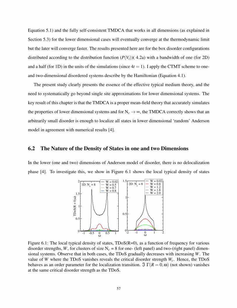
Equation 5.1) and the fully self-consistent TMDCA that works in all dimensions (as explained in
Section 5.3) for the lower dimensional cases will eventually converge at the thermodynamic limit
but the later will converge faster. The results presented here are for the box disorder configurations
distributed according to the distribution function (P(Vi))( 4.2a) with a bandwidth of one (for 2D)
and a half (for 1D) in the units of the simulations (since 4t = 1). I apply the CTMT scheme to one-
and two-dimensional disordered systems describe by the Hamiltonian (Equation 4.1).
The present study clearly presents the essence of the effective typical medium theory, and the
need to systematically go beyond single site approximations for lower dimensional systems. The
key result of this chapter is that the TMDCA is a proper mean-field theory that accurately simulates
the properties of lower dimensional systems and for Nc → ∞, the TMDCA correctly shows that an
arbitrarily small disorder is enough to localize all states in lower dimensional ‘random’ Anderson
model in agreement with numerical results [4].
6.2 The Nature of the Density of States in one and two Dimensions
In the lower (one and two) dimensions of Anderson model of disorder, there is no delocalization
phase [4]. To investigate this, we show in Figure 6.1 shows the local typical density of states
-2 -1 0 1 2ω
0
0.5
1
1.5 W = 0.02W = 0.8W = 1.2W = 1.8W = 2.0
-1 -0.5 0 0.5 1ω
0
0.5
1
1.5
2
TD
oS
(R =
0;ω
)
W = 0.02W = 0.5W = 0.7W = 0.8
1D: Nc = 8 2D: N
c = 8
Figure 6.1: The local typical density of states, TDoS(R=0), as a function of frequency for various
disorder strengths, W , for clusters of size Nc = 8 for one- (left panel) and two-(right panel) dimen-
sional systems. Observe that in both cases, the TDoS gradually decreases with increasing W . The
value of W where the TDoS vanishes reveals the critical disorder strength Wc. Hence, the TDoS
behaves as an order parameter for the localization transition. ℑ Γ(R = 0,ω) (not shown) vanishes
at the same critical disorder strength as the TDoS.
57
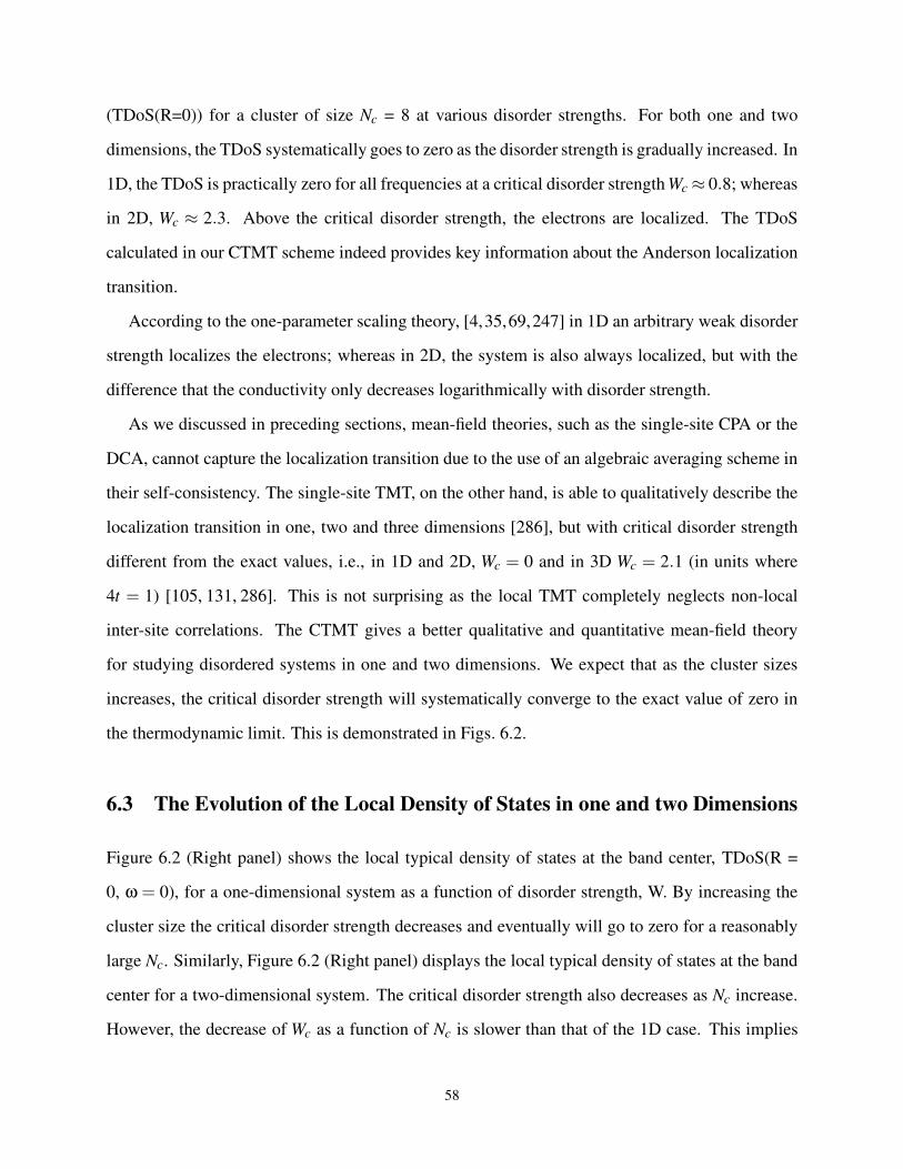
(TDoS(R=0)) for a cluster of size Nc = 8 at various disorder strengths. For both one and two
dimensions, the TDoS systematically goes to zero as the disorder strength is gradually increased. In
1D, the TDoS is practically zero for all frequencies at a critical disorder strength Wc ≈ 0.8; whereas
in 2D, Wc ≈ 2.3. Above the critical disorder strength, the electrons are localized. The TDoS
calculated in our CTMT scheme indeed provides key information about the Anderson localization
transition.
According to the one-parameter scaling theory, [4,35,69,247] in 1D an arbitrary weak disorder
strength localizes the electrons; whereas in 2D, the system is also always localized, but with the
difference that the conductivity only decreases logarithmically with disorder strength.
As we discussed in preceding sections, mean-field theories, such as the single-site CPA or the
DCA, cannot capture the localization transition due to the use of an algebraic averaging scheme in
their self-consistency. The single-site TMT, on the other hand, is able to qualitatively describe the
localization transition in one, two and three dimensions [286], but with critical disorder strength
different from the exact values, i.e., in 1D and 2D, Wc = 0 and in 3D Wc = 2.1 (in units where
4t = 1) [105, 131, 286]. This is not surprising as the local TMT completely neglects non-local
inter-site correlations. The CTMT gives a better qualitative and quantitative mean-field theory
for studying disordered systems in one and two dimensions. We expect that as the cluster sizes
increases, the critical disorder strength will systematically converge to the exact value of zero in
the thermodynamic limit. This is demonstrated in Figs. 6.2.
6.3 The Evolution of the Local Density of States in one and two Dimensions
Figure 6.2 (Right panel) shows the local typical density of states at the band center, TDoS(R =
0, ω = 0), for a one-dimensional system as a function of disorder strength, W. By increasing the
cluster size the critical disorder strength decreases and eventually will go to zero for a reasonably
large Nc. Similarly, Figure 6.2 (Right panel) displays the local typical density of states at the band
center for a two-dimensional system. The critical disorder strength also decreases as Nc increase.
However, the decrease of Wc as a function of Nc is slower than that of the 1D case. This implies
58

0 0.5 1 1.5 2W
0
0.2
0.4
0.6
TD
oS
(R =
0, ω
=0
)N
c = 1
Nc = 4
Nc = 8
Nc = 20
0 0.5 1W
0
0.1
0.2
Γ(R
=0
, ω
=0
)
1D
0 0.5 1 1.5 2 2.5W
0
0.5
1
TD
oS
(R =
0, ω
=0)
Nc = 8
Nc = 18
Nc = 32
Nc = 64
0 0.5 1 1.5 2 2.5W
0
0.1
0.2
Γ(R
=0, ω
=0)
2D
Figure 6.2: The local typical density of states at the band center, TDoS(R = 0, ω= 0), as a function
of disorder strength, W/4t, for various cluster sizes for 1D (Left panel) and 2D (Right panel). The
critical disorder strength Wc decreases exponentially (in 1D) and logarithmically (in 2D) as cluster
size Nc increases. The insets display the local hybridization rate at the band center Γ(R = 0,ω= 0)vs. W/4t. Note that Γ(R = 0,ω = 0) and TDoS(R=0, ω = 0) go to zero at the same critical disorder
strength.
that the scaling form of Wc vs Nc (or Lc) for 1D and 2D systems is different. The former follows
a power-law whereas the latter has a logarithmic form. This is consistent with the one-parameter
scaling theory [4, 35, 69, 247], which shows that a 1D system is strongly localized, while 2D is the
lower critical dimension of the Anderson localization transition. The insets of Figs. 6.2 show that
the local hybridization rate at the band center, Γ(R = 0,ω = 0), goes to zero at the same value of
W than the TDoS.
6.4 Scaling of the Critical Disorder Strength
Figures 6.3 and 6.4 address the scaling of Wc vs Nc. In 1D, the scaling ansatz is ξ = Lc ∼ W−νc ,
where ξ is the localization length, and ν is the critical exponent. As shown in Figure 6.3, the
power law behavior is nicely captured by our data with 1/ν = 0.46± 0.10 in basic agreement
with numerical results which reported a value of 1/ν = 0.5 [288], and also with the one-parameter
scaling theory [4]. The inset of Figure 6.3 is a log log plot of disorder Wc vs cluster size Nc where
the power-law behavior Wc ∼ (1/Lc)1/ν is seen as a straight line depicting that Wc goes to zero for
large enough cluster size.
59
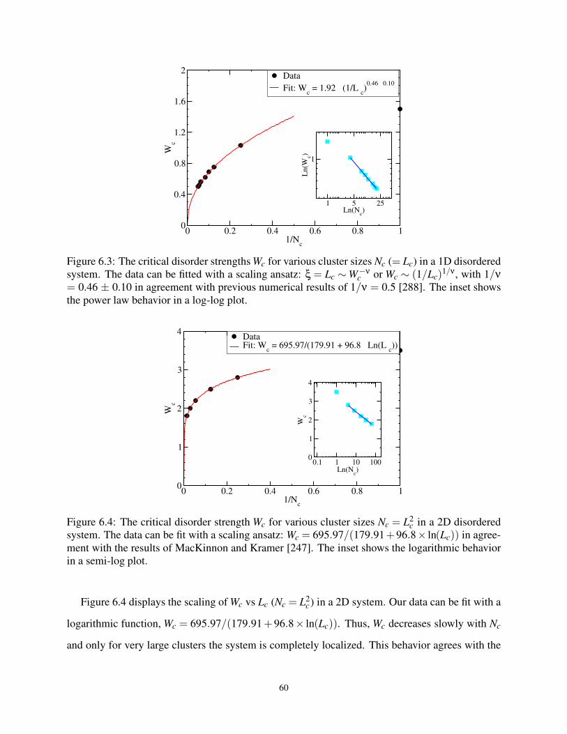
0 0.2 0.4 0.6 0.8 11/N
c
0
0.4
0.8
1.2
1.6
2
Wc
Data
Fit: Wc = 1.92 * (1/L
c)0.46 ± 0.10
1 5 25Ln(N
c)
1
Ln
(Wc)
Figure 6.3: The critical disorder strengths Wc for various cluster sizes Nc (= Lc) in a 1D disordered
system. The data can be fitted with a scaling ansatz: ξ = Lc ∼ W−νc or Wc ∼ (1/Lc)
1/ν, with 1/ν= 0.46 ± 0.10 in agreement with previous numerical results of 1/ν = 0.5 [288]. The inset shows
the power law behavior in a log-log plot.
0 0.2 0.4 0.6 0.8 11/N
c
0
1
2
3
4
Wc
DataFit: W
c= 695.97/(179.91 + 96.8 * Ln(L
c))
0.1 1 10 100Ln(N
c)
0
1
2
3
4
Wc
Figure 6.4: The critical disorder strength Wc for various cluster sizes Nc = L2c in a 2D disordered
system. The data can be fit with a scaling ansatz: Wc = 695.97/(179.91+96.8× ln(Lc)) in agree-
ment with the results of MacKinnon and Kramer [247]. The inset shows the logarithmic behavior
in a semi-log plot.
Figure 6.4 displays the scaling of Wc vs Lc (Nc = L2c) in a 2D system. Our data can be fit with a
logarithmic function, Wc = 695.97/(179.91+96.8× ln(Lc)). Thus, Wc decreases slowly with Nc
and only for very large clusters the system is completely localized. This behavior agrees with the
60

one-parameter scaling theory [4], as 2D is generally believed to be the lower critical dimension
for the ALT [289]. The inset of Figure 6.4 is a semi-log plot of Wc vs ln Nc where the logarithmic
behavior is seen as a straight line. We note that our data fit nicely to an exponent form: Lc =
exp(4.73/W 0.98c )/W 0.98
c in basic agreement with the results of MacKinnon and Kramer [247]. 1
6.5 The PDF for Lower Dimensional Anderson Localization
As explained in the previous sections, when system becomes localized, the PDFs of the density of
states change from Gaussian distribution (where all states are metallic, the PDF is symmetric with
the shape of TDoS the same as the ADoS) to a very asymmetric distribution with long tails (where
all states are localized, the LDoS strongly fluctuating at all sites, and the TDoS is very different
from the ADoS).
0 1 20
0.2
0.4
P[ρ
(K,ω
)] x
10
3
0 1 20
1
2
3
4
ABC
0 1 2 3 4
ρ(K,ω = εκ)
0
10
20
0 1 2
ρ(K,ω = εκ)
0
5
10
15
P[ρ
(K,ω
)] x
10
3
0 1 2
ρ(K,ω = εκ)
0
2
4
6
8
KEY K
0π/4π/2
(a) (b)
(c) (d) (e)
W = 0.2 W = 0.4
W = 0.5 W = 0.6 W = 0.8
0 0.2 0.40
1
2
P[ρ
(K,ω
)] x
10
3
0 0.4 0.80
0.5
1
1.5ABC
0 1 2
ρ(K,ω = εκ)
0
10
20
30
0 1 2
ρ(K,ω = εκ)
0
5
10
15
P[ρ
(K,ω
)] x
10
3
0 1 2
ρ(K,ω = εκ)
0
5
10
15
KEY Kx
Ky
-π/2 -π/20 0π 0
(a) (b)
(c) (d) (e)
W = 0.2W = 0.5
W = 1.0 W = 1.2 W = 1.8
Figure 6.5: The evolution of the probability distribution (PDF[ρ(K,ω = εK)]) at different cluster
cells with increasing W for a 1D system (Left Panel) and 2D system (Right Panel), the cluster size
is Nc = 8. The labels A–C correspond to three cluster momenta.
Utilizing large-scale exact diagonalization calculations, Schubert et al. [257] have demon-
strated that the PDFs close to the Anderson transition in 2D and 3D systems are log-normal. Here,
as a proof of principle, we perform similar calculations. Within the CTMT scheme, we obtain the
PDFs of the momentum-resolved DoS ρ(K,ω = εK) at different momenta cells centered at cluster
1The results obtained from the fully self-consistent, systematic TMDCA where Equation 5.11 is utilized in the self-consistent shows similar
trend. However, far smaller disorder strength (for e.g., for 1D at Nc = 64, for a disorder strength as small as 0.15,) is needed to localize all the states
in agreement with the single-parameter scaling [4]. For comparison, see Figs. 6.6 and 6.7 where the two methods are compared.
61
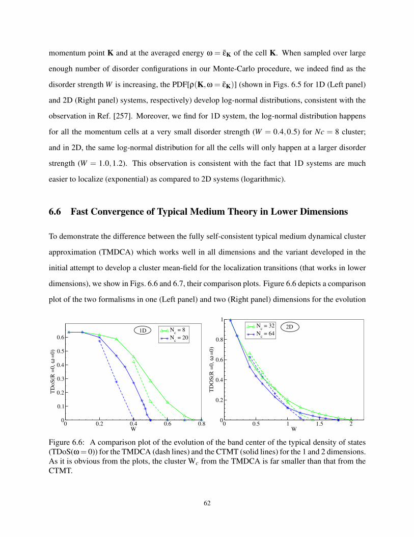
momentum point K and at the averaged energy ω = εK of the cell K. When sampled over large
enough number of disorder configurations in our Monte-Carlo procedure, we indeed find as the
disorder strength W is increasing, the PDF[ρ(K,ω = εK)] (shown in Figs. 6.5 for 1D (Left panel)
and 2D (Right panel) systems, respectively) develop log-normal distributions, consistent with the
observation in Ref. [257]. Moreover, we find for 1D system, the log-normal distribution happens
for all the momentum cells at a very small disorder strength (W = 0.4,0.5) for Nc = 8 cluster;
and in 2D, the same log-normal distribution for all the cells will only happen at a larger disorder
strength (W = 1.0,1.2). This observation is consistent with the fact that 1D systems are much
easier to localize (exponential) as compared to 2D systems (logarithmic).
6.6 Fast Convergence of Typical Medium Theory in Lower Dimensions
To demonstrate the difference between the fully self-consistent typical medium dynamical cluster
approximation (TMDCA) which works well in all dimensions and the variant developed in the
initial attempt to develop a cluster mean-field for the localization transitions (that works in lower
dimensions), we show in Figs. 6.6 and 6.7, their comparison plots. Figure 6.6 depicts a comparison
plot of the two formalisms in one (Left panel) and two (Right panel) dimensions for the evolution
0 0.2 0.4 0.6 0.8W
0
0.1
0.2
0.3
0.4
0.5
0.6
TD
oS
(R =
0, ω
=0
)
Nc = 8
Nc = 20
1D
0 0.5 1 1.5 2W
0
0.2
0.4
0.6
0.8
1
TD
OS
(R =
0, ω
=0
)
Nc = 32
Nc = 64
2D
Figure 6.6: A comparison plot of the evolution of the band center of the typical density of states
(TDoS(ω= 0)) for the TMDCA (dash lines) and the CTMT (solid lines) for the 1 and 2 dimensions.
As it is obvious from the plots, the cluster Wc from the TMDCA is far smaller than that from the
CTMT.
62
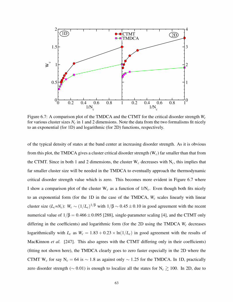
0.2 0.4 0.6 0.8 11/N
c
0
1
2
3
4CTMTTMDCA
0 0.2 0.4 0.6 0.8 11/N
c
0
0.5
1
1.5
2
Wc
1D 2D
Figure 6.7: A comparison plot of the TMDCA and the CTMT for the critical disorder strength Wc
for various cluster sizes Nc in 1 and 2 dimensions. Note the data from the two formalisms fit nicely
to an exponential (for 1D) and logarithmic (for 2D) functions, respectively.
of the typical density of states at the band center at increasing disorder strength. As it is obvious
from this plot, the TMDCA gives a cluster critical disorder strength (Wc) far smaller than that from
the CTMT. Since in both 1 and 2 dimensions, the cluster Wc decreases with Nc, this implies that
far smaller cluster size will be needed in the TMDCA to eventually approach the thermodynamic
critical disorder strength value which is zero. This becomes more evident in Figure 6.7 where
I show a comparison plot of the cluster Wc as a function of 1/Nc. Even though both fits nicely
to an exponential form (for the 1D in the case of the TMDCA, Wc scales linearly with linear
cluster size (Lc=Nc): Wc ∼ (1/Lc)1/β with 1/β ∼ 0.45± 0.10 in good agreement with the recent
numerical value of 1/β = 0.466±0.095 [288], single-parameter scaling [4], and the CTMT only
differing in the coefficients) and logarithmic form (for the 2D using the TMDCA Wc decreases
logarithmically with Lc as Wc = 1.83+ 0.23× ln(1/Lc) in good agreement with the results of
MacKinnon et al. [247]. This also agrees with the CTMT differing only in their coefficients)
(fitting not shown here), the TMDCA clearly goes to zero faster especially in the 2D where the
CTMT Wc for say Nc = 64 is ∼ 1.8 as against only ∼ 1.25 for the TMDCA. In 1D, practically
zero disorder strength (∼ 0.01) is enough to localize all the states for Nc & 100. In 2D, due to
63

the logarithmic nature of the decay of the Wc with 1/Nc, a large cluster is needed to achieve
the thermodynamic Wc. Hence, the TMDCA is in better agreement with the single-parameter
scaling theory which demonstrates that there is no delocalization phase in one and two-dimensional
systems, respectively, for the orthogonal universality class [4], and, therefore, a vanishing static
conductivity at zero temperature [290].
6.7 Conclusion
A cluster extension to the local typical medium theory via the dynamical cluster approximation for
studying localization in low dimensional disordered electronic systems have been developed. The
developed CTMT systematically incorporates non-local corrections to capture quantum coherence.
The formalism recovers the local TMT when the cluster size is Nc = 1 and becomes exact as Nc →
∞. As demonstrated, for the proper treatment of the lower dimensional systems, the local part of
the typical density of states should be separated and treated explicitly with geometrical averaging.
This way, cluster self-averaging which is manifestly more pronounced in three dimensions will
be avoided. The typical medium dynamical cluster approximation not only reproduces known
characteristics of the lower dimensional systems, for e.g., all states being localized for large system
size Nc → ∞ but opens a new avenue to study localization effects in lower dimensional model
systems.
64
Chapter 7
Application of Typical Medium Dynamical
Cluster Approximation to
Three-Dimensional Disordered System
This chapter comprises of two recently published papers:
“A Typical Medium Dynamical Cluster Approximation for the Study of Anderson Local-
ization in Three Dimensions”, Phys. Rev. B Rapid Commun. 89 081107 (2014). The
list of the authors, as it appears in the manuscript are C. E. Ekuma, H. Terletska, K.-M.
Tam, Z.-Y. Meng, J. Moreno, and M. Jarrell.;
“Finite cluster typical medium theory for disordered electronic systems”, (Manuscript
in preparation). The list of the authors, as it appears in the manuscript are C. E. Ekuma,
C. Moore, H. Terletska, K-M. Tam, J. Moreno, M. Jarrell, and N.S. Vidhyadhiraja.
My role is the development of the model, writing and debugging the code, implemen-
tation of the parallel version, running the code to generate the data and writing the
manuscript. The numerical exact methods (the exact diagonalization, transfer matrix,
and the kernel polynomial methods) which we benchmarked the TMDCA with is devel-
oped by my co-authors Conrad Moore and Ka Ming Tam.
7.1 Introduction
Unlike the lower dimensional systems, the non-interacting three-dimensional system intrinsically,
exhibits metal-insulator transitions (MIT) at a given critical disorder strength. Over the past sev-
eral decades, various mean-field models and methods have been developed and/or proposed to
characterize the localization transitions in three dimensions (see Chapter 4). The hallmark of these
65
mean-fields is their inability to properly characterize the Anderson localization in three dimen-
sions. As a consequence of this, a renewed search for new methods to better understand Anderson
localization [4, 35] remains an active area of the study of disordered electronic systems [44].
In this chapter, I will present the results from the typical medium dynamical cluster approxima-
tion (TMDCA) as applied to the non-interacting Anderson model. To reiterate, the TMDCA is a
systematic, self-consistent, causal, and computationally efficient algorithm the properly character-
izes the (Anderson) localization transitions not just in three dimensions but in lower (one and two)
dimensional systems. By a systematic increment of the cluster size (Nc → ∞), I will demonstrate
using various disorder distributions: Box, Gaussian, Lorentzian, and Alloy model (see Eqs 4.2)
that the typical density of states (or the hybridization rate) is a proper order parameter for charac-
terizing localization transitions. Furthermore, I will benchmark the TMDCA (which is for a small
finite cluster) to the numerically exact methods (which requires the simulation of very large lattice
cluster), and show, for instance, that the critical disorder strength obtained from the TMDCA is
numerically equivalent to that from the generally more computational expensive exact numerical
methods for the various disorder distributions.
To demonstrate the importance of the effective environment for a proper description of the
localization transitions, I will show using the DCA its inability to capture localization transitions.
Despite the systematic incorporation of spatial correlations in the DCA and such has several advan-
tages over the CPA, it shares the same behavior with the CPA as regards properly, characterizing
the localization transition in a disordered electron system. The inability of the DCA to capture
Anderson localization transition will be demonstrated using the box disorder distribution.
7.2 Absence of Localization in Dynamical Cluster Approximation
The dynamical cluster approximation (DCA) unlike the coherent potential approximation (CPA)
incorporates non-local spatial correlations systematically as the size of the cluster are increased.
While spatial correlation is an important ingredient in the localization transition in disordered
electron systems, the DCA effective medium is characterized by arithmetic averaging over the
66
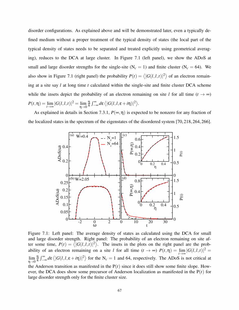
disorder configurations. As explained above and will be demonstrated later, even a typically de-
fined medium without a proper treatment of the typical density of states (the local part of the
typical density of states needs to be separated and treated explicitly using geometrical averag-
ing), reduces to the DCA at large cluster. In Figure 7.1 (left panel), we show the ADoS at
small and large disorder strengths for the single-site (Nc = 1) and finite cluster (Nc = 64). We
also show in Figure 7.1 (right panel) the probability P(t) =⟨|G(l, l, t)|2
⟩of an electron remain-
ing at a site say l at long time t calculated within the single-site and finite cluster DCA scheme
while the insets depict the probability of an electron remaining on site l for all time (t → ∞)
P(t,η) = limt→∞
|G(l, l, t)|2 = limη→0
ηπ
∫ ∞−∞ dε
⟨|G(l, l,ε+ iη)|2
⟩.
As explained in details in Section 7.3.1, P(∞,η) is expected to be nonzero for any fraction of
the localized states in the spectrum of the eigenstates of the disordered system [70, 218, 264, 266].
0
0.2
0.4
AD
oS
(ω)
0 0.2 0.4η
0
0.2
0.4
0.6
P(∞
,η)
-2 0 2ω
0
0.05
0.1
0.15
0.2
0.25
AD
oS
(ω)
0 10 20 30t
0
0.5
1
1.5P
(t)
0
0.5
1
1.5
P(t
)
0 0.2 0.4η
0
0.4
0.8
P(∞
,η)
Nc=1
Nc=64
(a) (c)
(b) (d)
W=0.4
W=2.05
Figure 7.1: Left panel: The average density of states as calculated using the DCA for small
and large disorder strength. Right panel: The probability of an electron remaining on site af-
ter some time, P(t) =⟨|G(l, l, t)|2
⟩. The insets in the plots on the right panel are the prob-
ability of an electron remaining on a site l for all time (t → ∞) P(t,η) = limt→∞
|G(l, l, t)|2 =
limη→0
ηπ
∫ ∞−∞ dε
⟨|G(l, l,ε+ iη)|2
⟩for the Nc = 1 and 64, respectively. The ADoS is not critical at
the Anderson transition as manifested in the P(t) since it does still show some finite slope. How-
ever, the DCA does show some precursor of Anderson localization as manifested in the P(t) for
large disorder strength only for the finite cluster size.
67
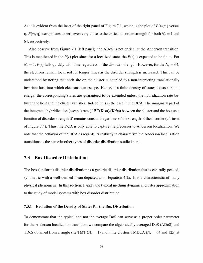
As it is evident from the inset of the right panel of Figure 7.1, which is the plot of P(∞,η) versus
η, P(∞,η) extrapolates to zero even very close to the critical disorder strength for both Nc = 1 and
64, respectively.
Also observe from Figure 7.1 (left panel), the ADoS is not critical at the Anderson transition.
This is manifested in the P(t) plot since for a localized state, the P(t) is expected to be finite. For
Nc = 1, P(t) falls quickly with time regardless of the disorder strength. However, for the Nc = 64,
the electrons remain localized for longer times as the disorder strength is increased. This can be
understood by noting that each site on the cluster is coupled to a non-interacting translationally
invariant host into which electrons can escape. Hence, if a finite density of states exists at some
energy, the corresponding states are guaranteed to be extended unless the hybridization rate be-
tween the host and the cluster vanishes. Indeed, this is the case in the DCA. The imaginary part of
the integrated hybridization (escape) rate (∫
ℑΓ(K,ω)dKdω) between the cluster and the host as a
function of disorder strength W remains constant regardless of the strength of the disorder (cf. inset
of Figure 7.4). Thus, the DCA is only able to capture the precursor to Anderson localization. We
note that the behavior of the DCA as regards its inability to characterize the Anderson localization
transitions is the same in other types of disorder distribution studied here.
7.3 Box Disorder Distribution
The box (uniform) disorder distribution is a generic disorder distribution that is centrally peaked,
symmetric with a well-defined mean depicted as in Equation 4.2a. It is a characteristic of many
physical phenomena. In this section, I apply the typical medium dynamical cluster approximation
to the study of model systems with box disorder distribution.
7.3.1 Evolution of the Density of States for the Box Distribution
To demonstrate that the typical and not the average DoS can serve as a proper order parameter
for the Anderson localization transition, we compare the algebraically averaged DoS (ADoS) and
TDoS obtained from a single site TMT (Nc = 1) and finite clusters TMDCA (Nc = 64 and 125) at
68
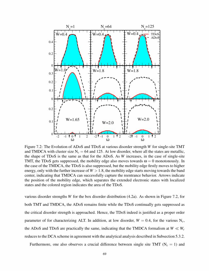
0
0.2
0.4
TDoSADoS
-2 -1 0 1 2ω
0
0.1
0.2
0
0.1
0.2
0.3
-2 -1 0 1 2ω
-2 -1 0 1 2ω
Nc=1 N
c=64 N
c=125
W=0.4 W=0.4 W=0.4
W=1.8W=1.8W=1.0
W=2.0W=2.0
W=1.65
Figure 7.2: The Evolution of ADoS and TDoS at various disorder strength W for single-site TMT
and TMDCA with cluster size Nc = 64 and 125. At low disorder, where all the states are metallic,
the shape of TDoS is the same as that for the ADoS. As W increases, in the case of single-site
TMT, the TDoS gets suppressed, the mobility edge also moves towards ω = 0 monotonously. In
the case of the TMDCA, the TDoS is also suppressed, but the mobility edge firstly moves to higher
energy, only with the further increase of W > 1.8, the mobility edge starts moving towards the band
center, indicating that TMDCA can successfully capture the reentrance behavior. Arrows indicate
the position of the mobility edge, which separates the extended electronic states with localized
states and the colored region indicates the area of the TDoS.
various disorder strengths W for the box disorder distribution (4.2a). As shown in Figure 7.2, for
both TMT and TMDCA, the ADoS remains finite while the TDoS continually gets suppressed as
the critical disorder strength is approached. Hence, the TDoS indeed is justified as a proper order
parameter of for characterizing ALT. In addition, at low disorder, W = 0.4, for the various Nc,
the ADoS and TDoS are practically the same, indicating that the TMDCA formalism at W ≪ Wc
reduces to the DCA scheme in agreement with the analytical analysis described in Subsection 5.3.2.
Furthermore, one also observes a crucial difference between single site TMT (Nc = 1) and
69
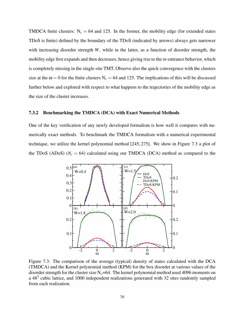
TMDCA finite clusters: Nc = 64 and 125. In the former, the mobility edge (for extended states
TDoS is finite) defined by the boundary of the TDoS (indicated by arrows) always gets narrower
with increasing disorder strength W , while in the latter, as a function of disorder strength, the
mobility edge first expands and then decreases, hence giving rise to the re-entrance behavior, which
is completely missing in the single-site TMT. Observe also the quick convergence with the clusters
size at the ω = 0 for the finite clusters Nc = 64 and 125. The implications of this will be discussed
further below and explored with respect to what happens to the trajectories of the mobility edge as
the size of the cluster increases.
7.3.2 Benchmarking the TMDCA (DCA) with Exact Numerical Methods
One of the key verification of any newly developed formalism is how well it compares with nu-
merically exact methods. To benchmark the TMDCA formalism with a numerical experimental
technique, we utilize the kernel polynomial method [245, 275]. We show in Figure 7.3 a plot of
the TDoS (ADoS) (Nc = 64) calculated using our TMDCA (DCA) method as compared to the
0
0.1
0.2
0.3
0.4
0.5
DoSTDoSDoS;KPMTDoS;KPM
0
0.1
0.2
-2 0 2ω
0
0.1
0.2
-2 0 2ω
0
0.1
0.2
(a) (c)
(b) (d)
W=0.4
W=1.8
W=1.5
W=2.0
Figure 7.3: The comparison of the average (typical) density of states calculated with the DCA
(TMDCA) and the Kernel polynomial method (KPM) for the box disorder at various values of the
disorder strength for the cluster size Nc=64. The kernel polynomial method used 4096 moments on
a 483 cubic lattice, and 1000 independent realizations generated with 32 sites randomly sampled
from each realization.
70
average and typical density of states obtained using the kernel polynomial method [245, 246]. As
it is evident from the plots, the agreement between the results from our method and the ones ob-
tained using the kernel polynomial method is remarkable. This good agreement is a manifestation
of the ability of our TMDCA formalism [2] to accurately characterize the Anderson localization
transitions in systems with uniform disorder distribution even with relatively small system size as
compared to the large lattice systems that need to be simulated in the kernel polynomial method
for accurate results to be obtained.
7.3.3 Exploring the effects of Finite Cluster on Critical Disorder Strength
Here, we consider the evolution of the critical disorder strength Wc with the cluster size. Figure 7.4
shows the TDoS(ω = 0) at the band center as a function of disorder strength W for several cluster
sizes: Nc = 1,64, and 125. The critical disorder strength Wc is defined by the vanishing of the
TDOS(ω= 0). The inset is the imaginary part of the integrated hybridization function which shares
the same property as the TDoS since both vanishes at the same disorder strength. Our results show
that as Nc increases, the critical disorder strength Wc systematically increases until it converges
to the exact value Wc ≈ 2.10 [131, 142, 242, 247, 270, 271, 275, 286] at cluster size Nc ≥ 12. The
cluster Nc = 12 is the first cluster with a complete nearest-neighbor shell based on Betts cluster
classification. [291] (cf. Appendix B. From this cluster onward, Wc converges to ≈ 2.10, but the
trajectory of the mobility edge continues to change until it also converges to the exact results at
larger Nc. This effect is due to the systematic incorporation of coherent backscattering as the cluster
size increases and will be elaborated in more detail later. To extract the order parameter critical
exponent (β), we fit our data in Figure 7.4 for the largest system size considered here (Nc = 125)
using the power law: TDoS(ω = 0) = a0|W −Wf it
c |β following the procedure as explained in
Subsection 7.7. We obtain β ∼ 1.62± 0.10 with a corresponding critical disorder strength from
the fit of Wf it
c ∼ 2.23±0.10. The critical parameters from the fit are in good agreement with the
recently reported value of β ≈ 1.67 [271]. It is also in general agreement with the values listed in
Table 7.2.
71
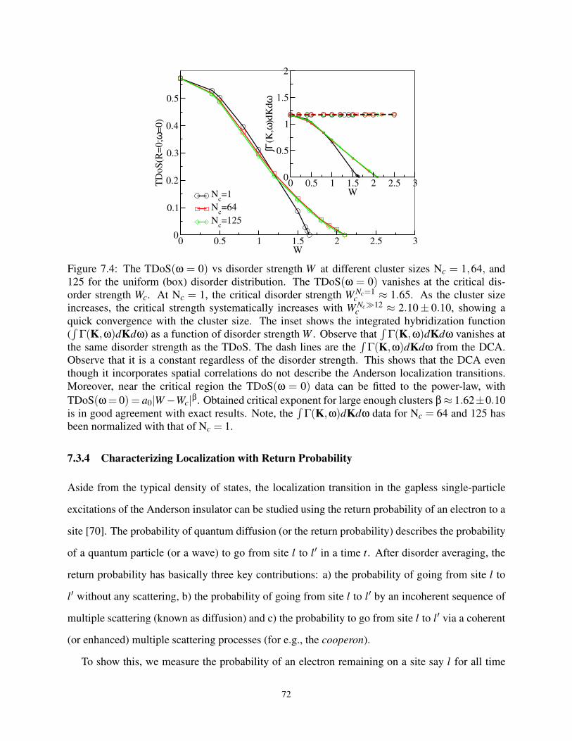
0 0.5 1 1.5 2 2.5 3W
0
0.1
0.2
0.3
0.4
0.5
TD
oS
(R=
0;ω
=0)
Nc=1
Nc=64
Nc=125
0 0.5 1 1.5 2 2.5 3W
0
0.5
1
1.5
2
∫Γ(K
,ω)d
Kdω
Figure 7.4: The TDoS(ω = 0) vs disorder strength W at different cluster sizes Nc = 1,64, and
125 for the uniform (box) disorder distribution. The TDoS(ω = 0) vanishes at the critical dis-
order strength Wc. At Nc = 1, the critical disorder strength W Nc=1c ≈ 1.65. As the cluster size
increases, the critical strength systematically increases with W Nc≫12c ≈ 2.10± 0.10, showing a
quick convergence with the cluster size. The inset shows the integrated hybridization function
(∫
Γ(K,ω)dKdω) as a function of disorder strength W . Observe that∫
Γ(K,ω)dKdω vanishes at
the same disorder strength as the TDoS. The dash lines are the∫
Γ(K,ω)dKdω from the DCA.
Observe that it is a constant regardless of the disorder strength. This shows that the DCA even
though it incorporates spatial correlations do not describe the Anderson localization transitions.
Moreover, near the critical region the TDoS(ω = 0) data can be fitted to the power-law, with
TDoS(ω= 0) = a0|W −Wc|β. Obtained critical exponent for large enough clusters β ≈ 1.62±0.10
is in good agreement with exact results. Note, the∫
Γ(K,ω)dKdω data for Nc = 64 and 125 has
been normalized with that of Nc = 1.
7.3.4 Characterizing Localization with Return Probability
Aside from the typical density of states, the localization transition in the gapless single-particle
excitations of the Anderson insulator can be studied using the return probability of an electron to a
site [70]. The probability of quantum diffusion (or the return probability) describes the probability
of a quantum particle (or a wave) to go from site l to l′ in a time t. After disorder averaging, the
return probability has basically three key contributions: a) the probability of going from site l to
l′ without any scattering, b) the probability of going from site l to l′ by an incoherent sequence of
multiple scattering (known as diffusion) and c) the probability to go from site l to l′ via a coherent
(or enhanced) multiple scattering processes (for e.g., the cooperon).
To show this, we measure the probability of an electron remaining on a site say l for all time
72
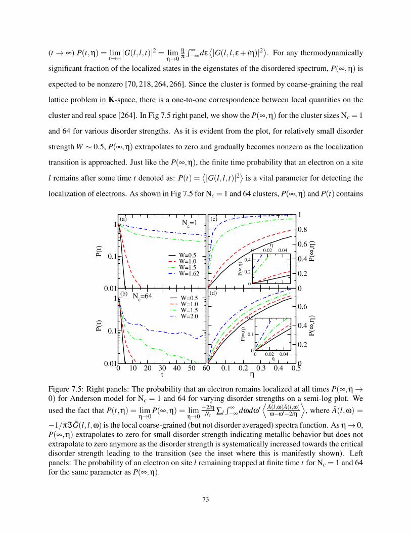
(t → ∞) P(t,η) = limt→∞
|G(l, l, t)|2 = limη→0
ηπ
∫ ∞−∞ dε
⟨|G(l, l,ε+ iη)|2
⟩. For any thermodynamically
significant fraction of the localized states in the eigenstates of the disordered spectrum, P(∞,η) is
expected to be nonzero [70, 218, 264, 266]. Since the cluster is formed by coarse-graining the real
lattice problem in K-space, there is a one-to-one correspondence between local quantities on the
cluster and real space [264]. In Fig 7.5 right panel, we show the P(∞,η) for the cluster sizes Nc = 1
and 64 for various disorder strengths. As it is evident from the plot, for relatively small disorder
strength W ∼ 0.5, P(∞,η) extrapolates to zero and gradually becomes nonzero as the localization
transition is approached. Just like the P(∞,η), the finite time probability that an electron on a site
l remains after some time t denoted as: P(t) =⟨|G(l, l, t)|2
⟩is a vital parameter for detecting the
localization of electrons. As shown in Fig 7.5 for Nc = 1 and 64 clusters, P(∞,η) and P(t) contains
0.01
0.1
1
P(t
)
W=0.5W=1.0W=1.5W=1.62
0 0.02 0.04η
0
0.2
0.4
P(∞
,η)
0 10 20 30 40 50 60t
0.01
0.1
1
P(t
)
W=0.5W=1.0W=1.5W=2.0
0 0.02 0.04η
0
0.1
0.2
P(∞
,η)
0 0.1 0.2 0.3 0.4 0.5η
0
0.2
0.4
0.6P
(∞,η
)
0
0.2
0.4
0.6
0.8
1
P(∞
,η)
Nc=1
Nc=64
(a) (c)
(b) (d)
Figure 7.5: Right panels: The probability that an electron remains localized at all times P(∞,η →0) for Anderson model for Nc = 1 and 64 for varying disorder strengths on a semi-log plot. We
used the fact that P(t,η) = limη→0
P(∞,η) = limη→0
−2iηNc
∑l
∫ ∞−∞ dωdω′
⟨A(l,ω)A(l,ω)ω−ω′−2iη
⟩
, where A(l,ω) =
−1/πℑG(l, l,ω) is the local coarse-grained (but not disorder averaged) spectra function. As η→ 0,
P(∞,η) extrapolates to zero for small disorder strength indicating metallic behavior but does not
extrapolate to zero anymore as the disorder strength is systematically increased towards the critical
disorder strength leading to the transition (see the inset where this is manifestly shown). Left
panels: The probability of an electron on site l remaining trapped at finite time t for Nc = 1 and 64
for the same parameter as P(∞,η).
73
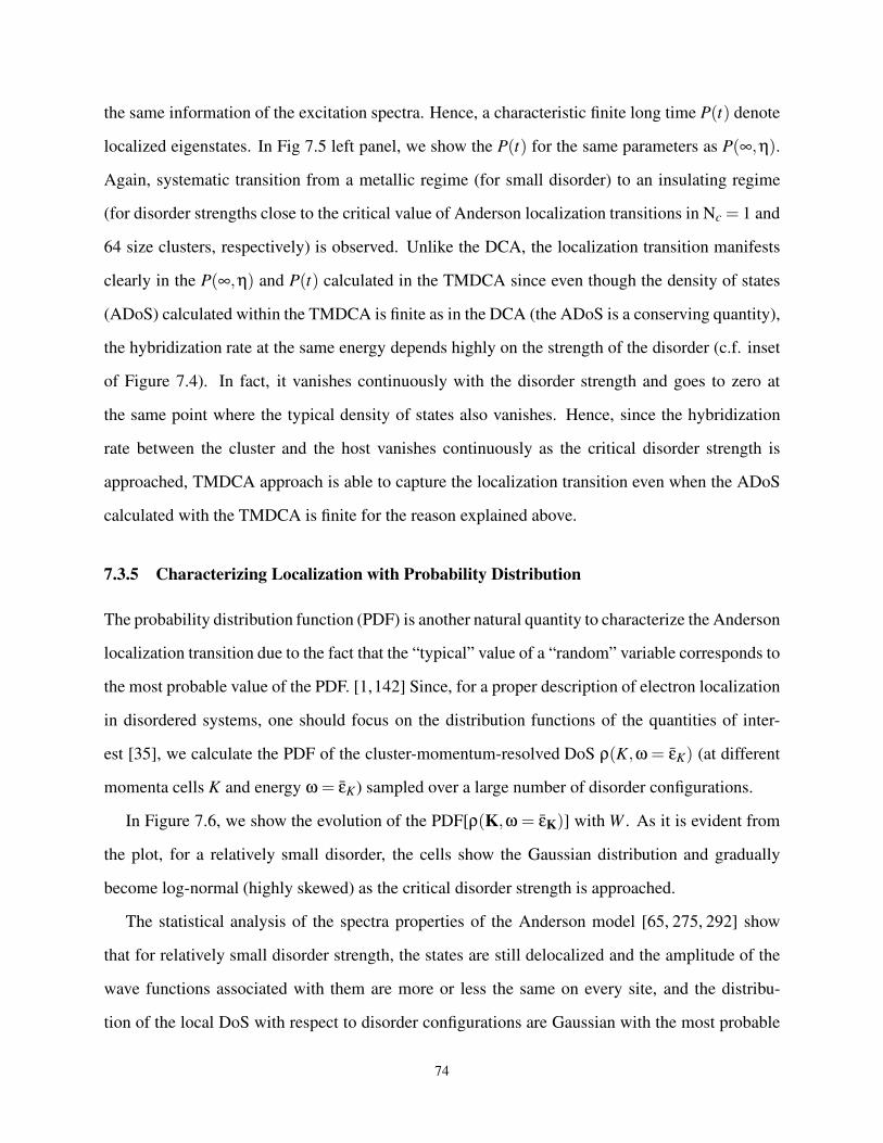
the same information of the excitation spectra. Hence, a characteristic finite long time P(t) denote
localized eigenstates. In Fig 7.5 left panel, we show the P(t) for the same parameters as P(∞,η).
Again, systematic transition from a metallic regime (for small disorder) to an insulating regime
(for disorder strengths close to the critical value of Anderson localization transitions in Nc = 1 and
64 size clusters, respectively) is observed. Unlike the DCA, the localization transition manifests
clearly in the P(∞,η) and P(t) calculated in the TMDCA since even though the density of states
(ADoS) calculated within the TMDCA is finite as in the DCA (the ADoS is a conserving quantity),
the hybridization rate at the same energy depends highly on the strength of the disorder (c.f. inset
of Figure 7.4). In fact, it vanishes continuously with the disorder strength and goes to zero at
the same point where the typical density of states also vanishes. Hence, since the hybridization
rate between the cluster and the host vanishes continuously as the critical disorder strength is
approached, TMDCA approach is able to capture the localization transition even when the ADoS
calculated with the TMDCA is finite for the reason explained above.
7.3.5 Characterizing Localization with Probability Distribution
The probability distribution function (PDF) is another natural quantity to characterize the Anderson
localization transition due to the fact that the “typical” value of a “random” variable corresponds to
the most probable value of the PDF. [1,142] Since, for a proper description of electron localization
in disordered systems, one should focus on the distribution functions of the quantities of inter-
est [35], we calculate the PDF of the cluster-momentum-resolved DoS ρ(K,ω = εK) (at different
momenta cells K and energy ω = εK) sampled over a large number of disorder configurations.
In Figure 7.6, we show the evolution of the PDF[ρ(K,ω = εK)] with W . As it is evident from
the plot, for a relatively small disorder, the cells show the Gaussian distribution and gradually
become log-normal (highly skewed) as the critical disorder strength is approached.
The statistical analysis of the spectra properties of the Anderson model [65, 275, 292] show
that for relatively small disorder strength, the states are still delocalized and the amplitude of the
wave functions associated with them are more or less the same on every site, and the distribu-
tion of the local DoS with respect to disorder configurations are Gaussian with the most probable
74
0 0.04 0.08
ρ(K,ω = εκ)
0
2
4
0 0.04 0.08
ρ(K,ω = εκ)
0
1
2
P[ρ
(K,ω
)] x
10
3
0 0.04 0.08 0.120
0.5
1
P[ρ
(K,ω
)] x
10
3
0 0.05 0.1 0.150
0.5
1
ABCD
0 0.04 0.08
ρ(K,ω = εκ)
0
0.5
1
W = 0.2 W = 0.5
W = 1.0 W = 2.0
(b)(a)
(c) (e)
W = 1.5
(d)
-2.15 -1.49 -2.48-0.33 -2.65 -2.32
-2.980.000.00
1.320.00
-1.98
KEY Kx
Ky
Kz
Figure 7.6: The evolution of the probability distribution of the density of states at different cluster
cells with an increase of disorder strength for Nc = 38. Utilizing the irreducible wedge property
and particle-hole symmetry, the original 38 cells is reduced to 4 cells. For small disorder strength,
the cells show Gaussian distribution and close to the critical disorder strength ≃ 2.0, all the cells
show log-normal distribution.
value coinciding with the arithmetic mean (average) value. However, for sufficiently large disorder
strength or in the proximity of the band tails, the spectrum consist mainly of discrete eigenvalues,
and the associated eigenfunctions are exponentially localized with only substantial weight only on
a few sites. The distribution is therefore extremely asymmetric (log-normal form), with a most
probable value much smaller than the arithmetic mean value. At this point, most of the weight is
concentrated around zero. As it is evident from Figure 7.6, we indeed observe such behavior in
our results.
7.3.6 The Phase Diagram for Anderson Model
The phase diagram in the disorder-energy (W-ω) plane for the 3D is one of the most important
tools for characterizing the Anderson localization transition. We show in Figure 7.7, the phase
diagram of the Anderson localization transitions in the (W-ω) plane constructed from our TMDCA
procedure for the box disorder distribution. Here, we show the mobility edge trajectories given
75
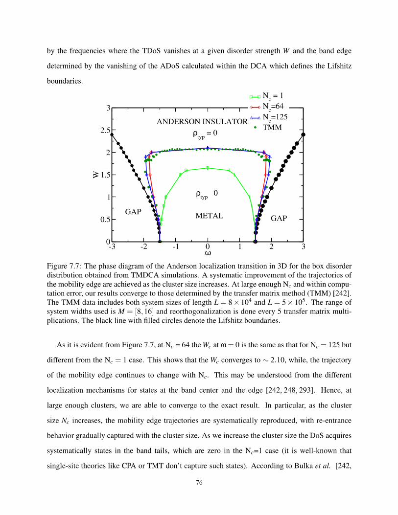
by the frequencies where the TDoS vanishes at a given disorder strength W and the band edge
determined by the vanishing of the ADoS calculated within the DCA which defines the Lifshitz
boundaries.
-3 -2 -1 0 1 2 3ω
0
0.5
1
1.5
2
2.5
3
WN
c = 1
Nc=64
Nc=125
TMM
GAPGAPMETAL
ρtyp
> 0
ANDERSON INSULATOR
ρtyp
= 0
Figure 7.7: The phase diagram of the Anderson localization transition in 3D for the box disorder
distribution obtained from TMDCA simulations. A systematic improvement of the trajectories of
the mobility edge are achieved as the cluster size increases. At large enough Nc and within compu-
tation error, our results converge to those determined by the transfer matrix method (TMM) [242].
The TMM data includes both system sizes of length L = 8× 10⁴ and L = 5× 10⁵. The range of
system widths used is M = [8,16] and reorthogonalization is done every 5 transfer matrix multi-
plications. The black line with filled circles denote the Lifshitz boundaries.
As it is evident from Figure 7.7, at Nc = 64 the Wc at ω = 0 is the same as that for Nc = 125 but
different from the Nc = 1 case. This shows that the Wc converges to ∼ 2.10, while, the trajectory
of the mobility edge continues to change with Nc. This may be understood from the different
localization mechanisms for states at the band center and the edge [242, 248, 293]. Hence, at
large enough clusters, we are able to converge to the exact result. In particular, as the cluster
size Nc increases, the mobility edge trajectories are systematically reproduced, with re-entrance
behavior gradually captured with the cluster size. As we increase the cluster size the DoS acquires
systematically states in the band tails, which are zero in the Nc=1 case (it is well-known that
single-site theories like CPA or TMT don’t capture such states). According to Bulka et al. [242,
76
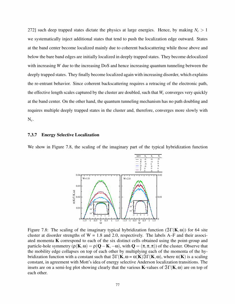
272] such deep trapped states dictate the physics at large energies. Hence, by making Nc > 1
we systematically inject additional states that tend to push the localization edge outward. States
at the band center become localized mainly due to coherent backscattering while those above and
below the bare band edges are initially localized in deeply trapped states. They become delocalized
with increasing W due to the increasing DoS and hence increasing quantum tunneling between the
deeply trapped states. They finally become localized again with increasing disorder, which explains
the re-entrant behavior. Since coherent backscattering requires a retracing of the electronic path,
the effective length scales captured by the cluster are doubled, such that Wc converges very quickly
at the band center. On the other hand, the quantum tunneling mechanism has no path doubling and
requires multiple deeply trapped states in the cluster and, therefore, converges more slowly with
Nc.
7.3.7 Energy Selective Localization
We show in Figure 7.8, the scaling of the imaginary part of the typical hybridization function
-1.5 -1 -0.5 0 0.5 1 1.5ω
0
0.01
0.02
0.03
0.04
α(K
)Γ(K
,ω)
ABCDEF
-2 -1 0 1 2
10-4
10-3
10-2
-2 -1 0 1 210
-4
10-3
10-2
-1.5 -1 -0.5 0 0.5 1 1.5ω
0
0.01
0.02
KEY Kx
Ky
Kz
-π/2 -π/2 -π/2-π/2-π/2-π/200
-π/20π0
π
πππ0
π
W=1.8 W=2.0
Figure 7.8: The scaling of the imaginary typical hybridization function (ℑΓ(K,ω)) for 64 site
cluster at disorder strengths of W = 1.8 and 2.0, respectively. The labels A–F and their associ-
ated momenta K correspond to each of the six distinct cells obtained using the point-group and
particle-hole symmetry (ρ(K,ω) = ρ(Q−K,−ω), with Q = (π,π,π)) of the cluster. Observe that
the mobility edge collapses on top of each other by multiplying each of the momenta of the hy-
bridization function with a constant such that ℑΓ(K,ω = α(K)ℑΓ(K,ω), where α(K) is a scaling
constant, in agreement with Mott’s idea of energy selective Anderson localization transitions. The
insets are on a semi-log plot showing clearly that the various K-values of ℑΓ(K,ω) are on top of
each other.
77
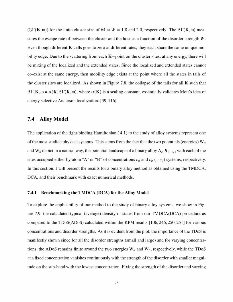
(ℑΓ(K,ω)) for the finite cluster size of 64 at W = 1.8 and 2.0, respectively. The ℑΓ(K,ω) mea-
sures the escape rate of between the cluster and the host as a function of the disorder strength W .
Even though different K-cells goes to zero at different rates, they each share the same unique mo-
bility edge. Due to the scattering from each K−point on the cluster sites, at any energy, there will
be mixing of the localized and the extended states. Since the localized and extended states cannot
co-exist at the same energy, then mobility edge exists at the point where all the states in tails of
the cluster sites are localized. As shown in Figure 7.8, the collapse of the tails for all K such that
ℑΓ(K,ω = α(K)ℑΓ(K,ω), where α(K) is a scaling constant, essentially validates Mott’s idea of
energy selective Anderson localization. [39, 116]
7.4 Alloy Model
The application of the tight-binding Hamiltonian ( 4.1) to the study of alloy systems represent one
of the most studied physical systems. This stems from the fact that the two potentials (energies) Wa
and Wb depict in a natural way, the potential landscape of a binary alloy AcaB1−ca
, with each of the
sites occupied either by atom “A” or “B” of concentrations ca and cb (1-ca) systems, respectively.
In this section, I will present the results for a binary alloy method as obtained using the TMDCA,
DCA, and their benchmark with exact numerical methods.
7.4.1 Benchmarking the TMDCA (DCA) for the Alloy Model
To explore the applicability of our method to the study of binary alloy systems, we show in Fig-
ure 7.9, the calculated typical (average) density of states from our TMDCA(DCA) procedure as
compared to the TDoS(ADoS) calculated within the KPM results [106, 246, 250, 251] for various
concentrations and disorder strengths. As it is evident from the plot, the importance of the TDoS is
manifestly shown since for all the disorder strengths (small and large) and for varying concentra-
tions, the ADoS remains finite around the two energies Wa and Wb, respectively, while the TDoS
at a fixed concentration vanishes continuously with the strength of the disorder with smaller magni-
tude on the sub-band with the lowest concentration. Fixing the strength of the disorder and varying
78
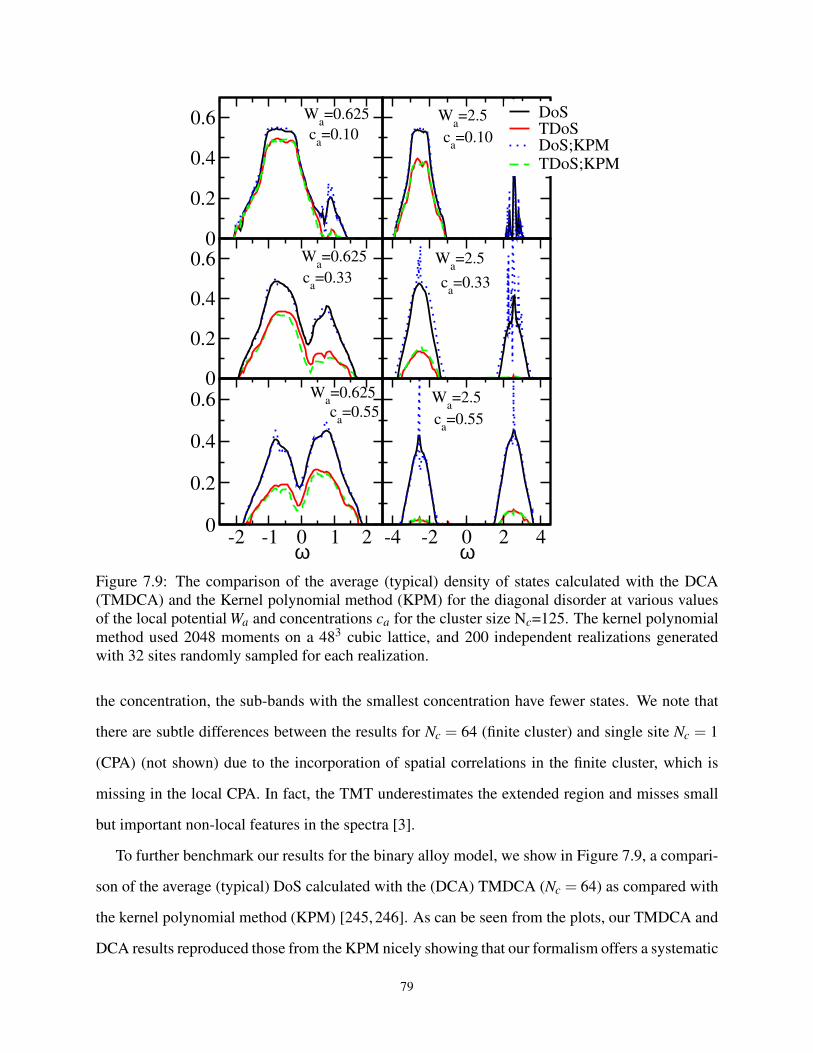
0
0.2
0.4
0.60
0.2
0.4
0.6 DoSTDoSDoS;KPMTDoS;KPM
-2 -1 0 1 2ω
0
0.2
0.4
0.6
-4 -2 0 2 4ω
ca=0.33
ca=0.55
Wa=0.625
Wa=2.5
Wa=2.5
Wa=2.5
Wa=0.625
ca=0.10
Wa=0.625
ca=0.10
ca=0.33
ca=0.55
Figure 7.9: The comparison of the average (typical) density of states calculated with the DCA
(TMDCA) and the Kernel polynomial method (KPM) for the diagonal disorder at various values
of the local potential Wa and concentrations ca for the cluster size Nc=125. The kernel polynomial
method used 2048 moments on a 483 cubic lattice, and 200 independent realizations generated
with 32 sites randomly sampled for each realization.
the concentration, the sub-bands with the smallest concentration have fewer states. We note that
there are subtle differences between the results for Nc = 64 (finite cluster) and single site Nc = 1
(CPA) (not shown) due to the incorporation of spatial correlations in the finite cluster, which is
missing in the local CPA. In fact, the TMT underestimates the extended region and misses small
but important non-local features in the spectra [3].
To further benchmark our results for the binary alloy model, we show in Figure 7.9, a compari-
son of the average (typical) DoS calculated with the (DCA) TMDCA (Nc = 64) as compared with
the kernel polynomial method (KPM) [245, 246]. As can be seen from the plots, our TMDCA and
DCA results reproduced those from the KPM nicely showing that our formalism offers a systematic
79
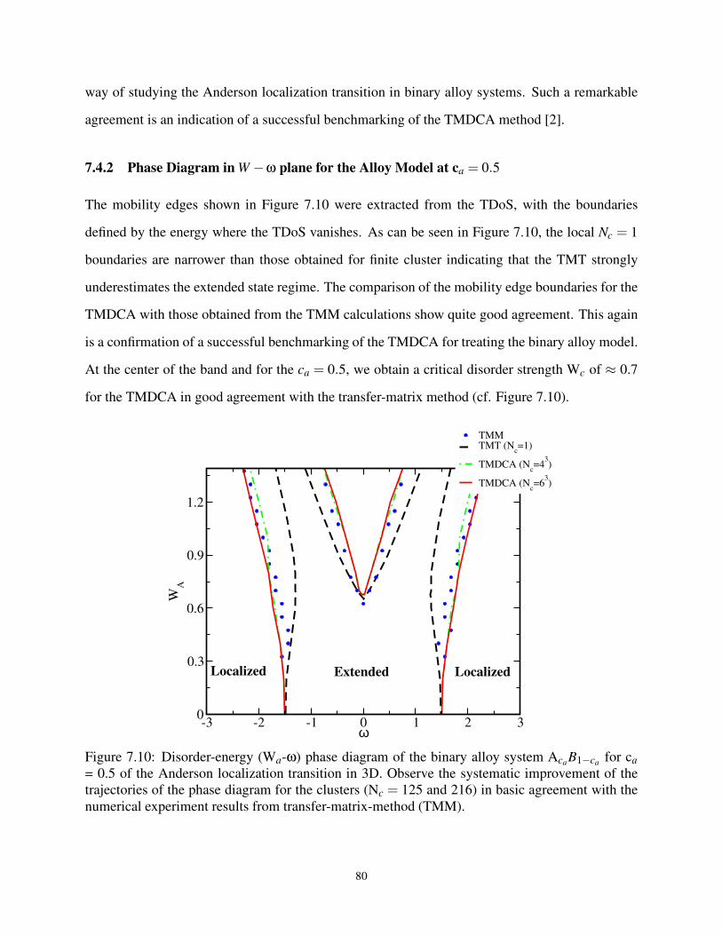
way of studying the Anderson localization transition in binary alloy systems. Such a remarkable
agreement is an indication of a successful benchmarking of the TMDCA method [2].
7.4.2 Phase Diagram in W −ω plane for the Alloy Model at ca = 0.5
The mobility edges shown in Figure 7.10 were extracted from the TDoS, with the boundaries
defined by the energy where the TDoS vanishes. As can be seen in Figure 7.10, the local Nc = 1
boundaries are narrower than those obtained for finite cluster indicating that the TMT strongly
underestimates the extended state regime. The comparison of the mobility edge boundaries for the
TMDCA with those obtained from the TMM calculations show quite good agreement. This again
is a confirmation of a successful benchmarking of the TMDCA for treating the binary alloy model.
At the center of the band and for the ca = 0.5, we obtain a critical disorder strength Wc of ≈ 0.7
for the TMDCA in good agreement with the transfer-matrix method (cf. Figure 7.10).
-3 -2 -1 0 1 2 3ω
0
0.3
0.6
0.9
1.2
WA
TMM TMT (N
c=1)
TMDCA (Nc=4
3)
TMDCA (Nc=6
3)
ExtendedLocalized Localized
Figure 7.10: Disorder-energy (Wa-ω) phase diagram of the binary alloy system AcaB1−ca
for ca
= 0.5 of the Anderson localization transition in 3D. Observe the systematic improvement of the
trajectories of the phase diagram for the clusters (Nc = 125 and 216) in basic agreement with the
numerical experiment results from transfer-matrix-method (TMM).
80
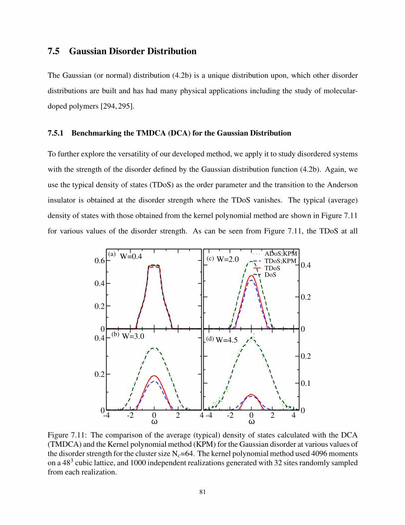
7.5 Gaussian Disorder Distribution
The Gaussian (or normal) distribution (4.2b) is a unique distribution upon, which other disorder
distributions are built and has had many physical applications including the study of molecular-
doped polymers [294, 295].
7.5.1 Benchmarking the TMDCA (DCA) for the Gaussian Distribution
To further explore the versatility of our developed method, we apply it to study disordered systems
with the strength of the disorder defined by the Gaussian distribution function (4.2b). Again, we
use the typical density of states (TDoS) as the order parameter and the transition to the Anderson
insulator is obtained at the disorder strength where the TDoS vanishes. The typical (average)
density of states with those obtained from the kernel polynomial method are shown in Figure 7.11
for various values of the disorder strength. As can be seen from Figure 7.11, the TDoS at all
0
0.2
0.4
0.6ADoS;KPMTDoS;KPMTDoSDoS
0
0.2
0.4
-4 -2 0 2 4ω
0
0.2
0.4
-4 -2 0 2 4ω
0
0.1
0.2
(a)(c)
(b)(d)
W=0.4
W=3.0
W=2.0
W=4.5
Figure 7.11: The comparison of the average (typical) density of states calculated with the DCA
(TMDCA) and the Kernel polynomial method (KPM) for the Gaussian disorder at various values of
the disorder strength for the cluster size Nc=64. The kernel polynomial method used 4096 moments
on a 483 cubic lattice, and 1000 independent realizations generated with 32 sites randomly sampled
from each realization.
81
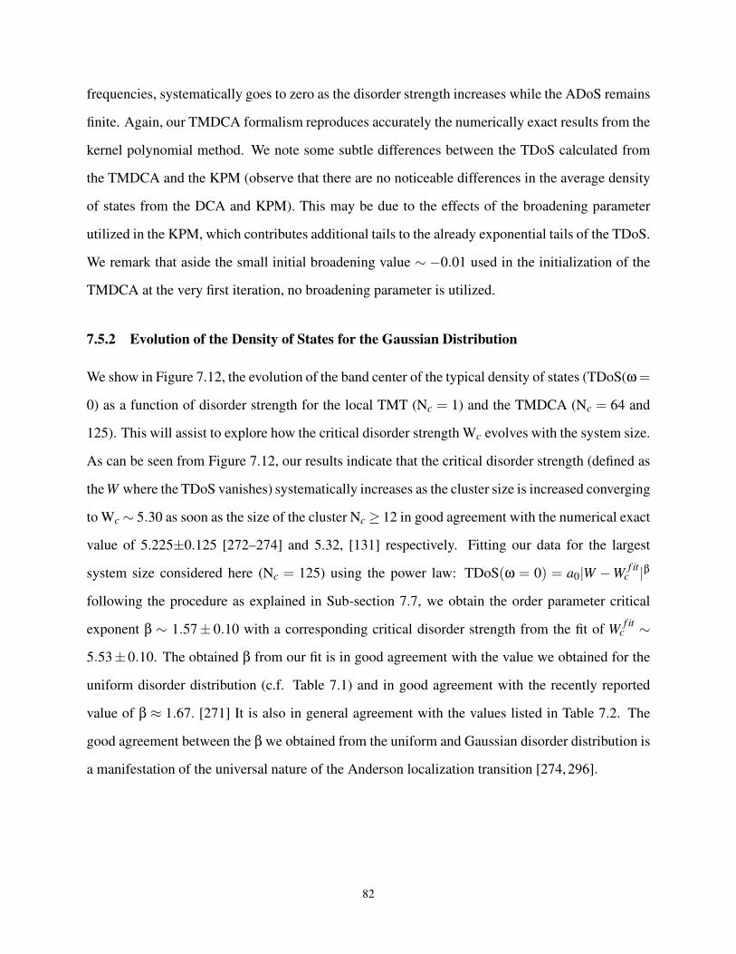
frequencies, systematically goes to zero as the disorder strength increases while the ADoS remains
finite. Again, our TMDCA formalism reproduces accurately the numerically exact results from the
kernel polynomial method. We note some subtle differences between the TDoS calculated from
the TMDCA and the KPM (observe that there are no noticeable differences in the average density
of states from the DCA and KPM). This may be due to the effects of the broadening parameter
utilized in the KPM, which contributes additional tails to the already exponential tails of the TDoS.
We remark that aside the small initial broadening value ∼ −0.01 used in the initialization of the
TMDCA at the very first iteration, no broadening parameter is utilized.
7.5.2 Evolution of the Density of States for the Gaussian Distribution
We show in Figure 7.12, the evolution of the band center of the typical density of states (TDoS(ω=
0) as a function of disorder strength for the local TMT (Nc = 1) and the TMDCA (Nc = 64 and
125). This will assist to explore how the critical disorder strength Wc evolves with the system size.
As can be seen from Figure 7.12, our results indicate that the critical disorder strength (defined as
the W where the TDoS vanishes) systematically increases as the cluster size is increased converging
to Wc ∼ 5.30 as soon as the size of the cluster Nc ≥ 12 in good agreement with the numerical exact
value of 5.225±0.125 [272–274] and 5.32, [131] respectively. Fitting our data for the largest
system size considered here (Nc = 125) using the power law: TDoS(ω = 0) = a0|W −Wf it
c |β
following the procedure as explained in Sub-section 7.7, we obtain the order parameter critical
exponent β ∼ 1.57± 0.10 with a corresponding critical disorder strength from the fit of Wf it
c ∼
5.53±0.10. The obtained β from our fit is in good agreement with the value we obtained for the
uniform disorder distribution (c.f. Table 7.1) and in good agreement with the recently reported
value of β ≈ 1.67. [271] It is also in general agreement with the values listed in Table 7.2. The
good agreement between the β we obtained from the uniform and Gaussian disorder distribution is
a manifestation of the universal nature of the Anderson localization transition [274, 296].
82
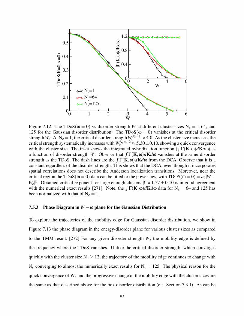
0 1 2 3 4 5 6W
0
0.1
0.2
0.3
0.4
0.5
TD
oS
(R=
0;ω
=0)
Nc=1
Nc=64
Nc=125
0 2 4 6W
0
0.4
0.8
1.2
∫Γ(K
,ω)d
Kdω
Figure 7.12: The TDoS(ω = 0) vs disorder strength W at different cluster sizes Nc = 1,64, and
125 for the Gaussian disorder distribution. The TDoS(ω = 0) vanishes at the critical disorder
strength Wc. At Nc = 1, the critical disorder strength W Nc=1c ≈ 4.0. As the cluster size increases, the
critical strength systematically increases with W Nc≫12c ≈ 5.30±0.10, showing a quick convergence
with the cluster size. The inset shows the integrated hybridization function (∫
Γ(K,ω)dKdω) as
a function of disorder strength W . Observe that∫
Γ(K,ω)dKdω vanishes at the same disorder
strength as the TDoS. The dash lines are the∫
Γ(K,ω)dKdω from the DCA. Observe that it is a
constant regardless of the disorder strength. This shows that the DCA, even though it incorporates
spatial correlations does not describe the Anderson localization transitions. Moreover, near the
critical region the TDoS(ω = 0) data can be fitted to the power-law, with TDOS(ω = 0) = a0|W −Wc|β. Obtained critical exponent for large enough clusters β ≈ 1.57± 0.10 is in good agreement
with the numerical exact results [271]. Note, the∫
Γ(K,ω)dKdω data for Nc = 64 and 125 has
been normalized with that of Nc = 1.
7.5.3 Phase Diagram in W −ω plane for the Gaussian Distribution
To explore the trajectories of the mobility edge for Gaussian disorder distribution, we show in
Figure 7.13 the phase diagram in the energy-disorder plane for various cluster sizes as compared
to the TMM result. [272] For any given disorder strength W , the mobility edge is defined by
the frequency where the TDoS vanishes. Unlike the critical disorder strength, which converges
quickly with the cluster size Nc ≥ 12, the trajectory of the mobility edge continues to change with
Nc converging to almost the numerically exact results for Nc = 125. The physical reason for the
quick convergence of Wc and the progressive change of the mobility edge with the cluster sizes are
the same as that described above for the box disorder distribution (c.f. Section 7.3.1). As can be
83
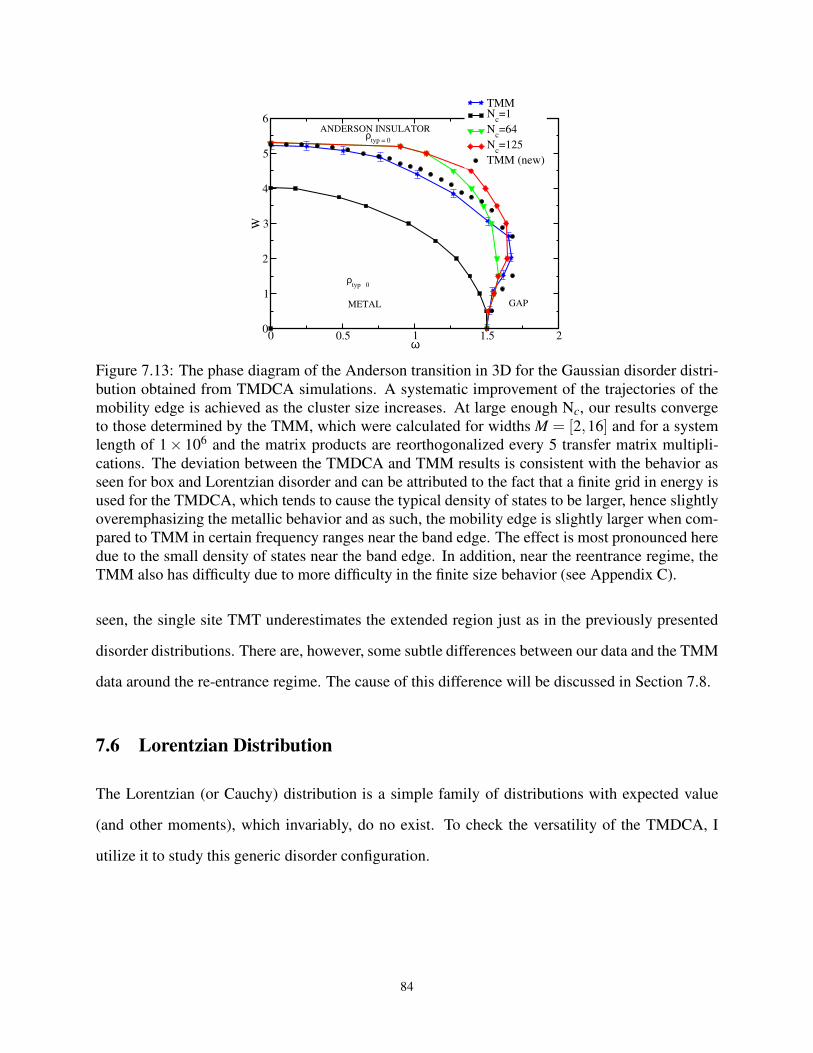
0 0.5 1 1.5 2ω
0
1
2
3
4
5
6
W
TMMN
c=1
Nc=64
Nc=125
TMM (new)
METAL GAP
ANDERSON INSULATOR
ρtyp > 0
ρtyp = 0
Figure 7.13: The phase diagram of the Anderson transition in 3D for the Gaussian disorder distri-
bution obtained from TMDCA simulations. A systematic improvement of the trajectories of the
mobility edge is achieved as the cluster size increases. At large enough Nc, our results converge
to those determined by the TMM, which were calculated for widths M = [2,16] and for a system
length of 1× 10⁶ and the matrix products are reorthogonalized every 5 transfer matrix multipli-
cations. The deviation between the TMDCA and TMM results is consistent with the behavior as
seen for box and Lorentzian disorder and can be attributed to the fact that a finite grid in energy is
used for the TMDCA, which tends to cause the typical density of states to be larger, hence slightly
overemphasizing the metallic behavior and as such, the mobility edge is slightly larger when com-
pared to TMM in certain frequency ranges near the band edge. The effect is most pronounced here
due to the small density of states near the band edge. In addition, near the reentrance regime, the
TMM also has difficulty due to more difficulty in the finite size behavior (see Appendix C).
seen, the single site TMT underestimates the extended region just as in the previously presented
disorder distributions. There are, however, some subtle differences between our data and the TMM
data around the re-entrance regime. The cause of this difference will be discussed in Section 7.8.
7.6 Lorentzian Distribution
The Lorentzian (or Cauchy) distribution is a simple family of distributions with expected value
(and other moments), which invariably, do no exist. To check the versatility of the TMDCA, I
utilize it to study this generic disorder configuration.
84
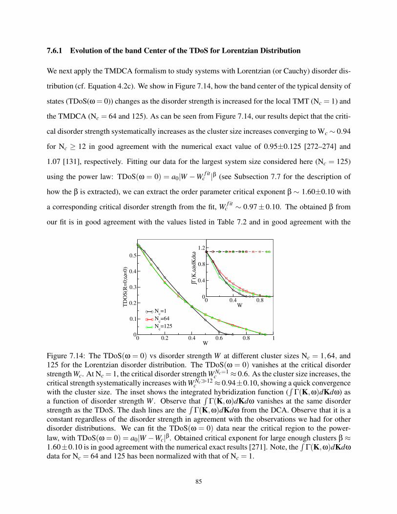
7.6.1 Evolution of the band Center of the TDoS for Lorentzian Distribution
We next apply the TMDCA formalism to study systems with Lorentzian (or Cauchy) disorder dis-
tribution (cf. Equation 4.2c). We show in Figure 7.14, how the band center of the typical density of
states (TDoS(ω = 0)) changes as the disorder strength is increased for the local TMT (Nc = 1) and
the TMDCA (Nc = 64 and 125). As can be seen from Figure 7.14, our results depict that the criti-
cal disorder strength systematically increases as the cluster size increases converging to Wc ∼ 0.94
for Nc ≥ 12 in good agreement with the numerical exact value of 0.95±0.125 [272–274] and
1.07 [131], respectively. Fitting our data for the largest system size considered here (Nc = 125)
using the power law: TDoS(ω = 0) = a0|W −Wf it
c |β (see Subsection 7.7 for the description of
how the β is extracted), we can extract the order parameter critical exponent β ∼ 1.60±0.10 with
a corresponding critical disorder strength from the fit, Wf it
c ∼ 0.97± 0.10. The obtained β from
our fit is in good agreement with the values listed in Table 7.2 and in good agreement with the
0 0.2 0.4 0.6 0.8 1W
0
0.1
0.2
0.3
0.4
0.5
TD
OS
(R=
0;ω
=0
)
Nc=1
Nc=64
Nc=125
0 0.4 0.8W
0
0.4
0.8
1.2
∫Γ(K
,ω)d
Kdω
Figure 7.14: The TDoS(ω = 0) vs disorder strength W at different cluster sizes Nc = 1,64, and
125 for the Lorentzian disorder distribution. The TDoS(ω = 0) vanishes at the critical disorder
strength Wc. At Nc = 1, the critical disorder strength W Nc=1c ≈ 0.6. As the cluster size increases, the
critical strength systematically increases with W Nc≫12c ≈ 0.94±0.10, showing a quick convergence
with the cluster size. The inset shows the integrated hybridization function (∫
Γ(K,ω)dKdω) as
a function of disorder strength W . Observe that∫
Γ(K,ω)dKdω vanishes at the same disorder
strength as the TDoS. The dash lines are the∫
Γ(K,ω)dKdω from the DCA. Observe that it is a
constant regardless of the disorder strength in agreement with the observations we had for other
disorder distributions. We can fit the TDoS(ω = 0) data near the critical region to the power-
law, with TDoS(ω = 0) = a0|W −Wc|β. Obtained critical exponent for large enough clusters β ≈1.60±0.10 is in good agreement with the numerical exact results [271]. Note, the
∫Γ(K,ω)dKdω
data for Nc = 64 and 125 has been normalized with that of Nc = 1.
85
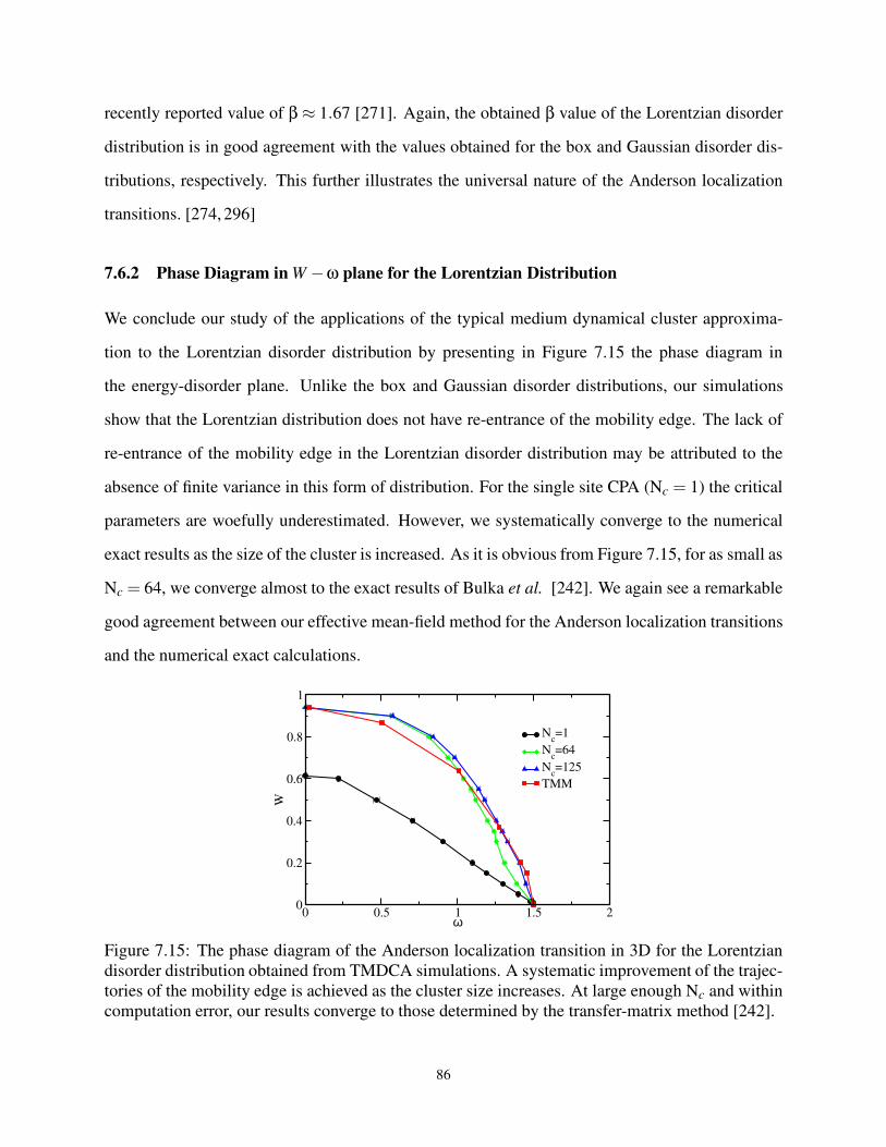
recently reported value of β ≈ 1.67 [271]. Again, the obtained β value of the Lorentzian disorder
distribution is in good agreement with the values obtained for the box and Gaussian disorder dis-
tributions, respectively. This further illustrates the universal nature of the Anderson localization
transitions. [274, 296]
7.6.2 Phase Diagram in W −ω plane for the Lorentzian Distribution
We conclude our study of the applications of the typical medium dynamical cluster approxima-
tion to the Lorentzian disorder distribution by presenting in Figure 7.15 the phase diagram in
the energy-disorder plane. Unlike the box and Gaussian disorder distributions, our simulations
show that the Lorentzian distribution does not have re-entrance of the mobility edge. The lack of
re-entrance of the mobility edge in the Lorentzian disorder distribution may be attributed to the
absence of finite variance in this form of distribution. For the single site CPA (Nc = 1) the critical
parameters are woefully underestimated. However, we systematically converge to the numerical
exact results as the size of the cluster is increased. As it is obvious from Figure 7.15, for as small as
Nc = 64, we converge almost to the exact results of Bulka et al. [242]. We again see a remarkable
good agreement between our effective mean-field method for the Anderson localization transitions
and the numerical exact calculations.
0 0.5 1 1.5 2ω
0
0.2
0.4
0.6
0.8
1
W
Nc=1
Nc=64
Nc=125
TMM
Figure 7.15: The phase diagram of the Anderson localization transition in 3D for the Lorentzian
disorder distribution obtained from TMDCA simulations. A systematic improvement of the trajec-
tories of the mobility edge is achieved as the cluster size increases. At large enough Nc and within
computation error, our results converge to those determined by the transfer-matrix method [242].
86
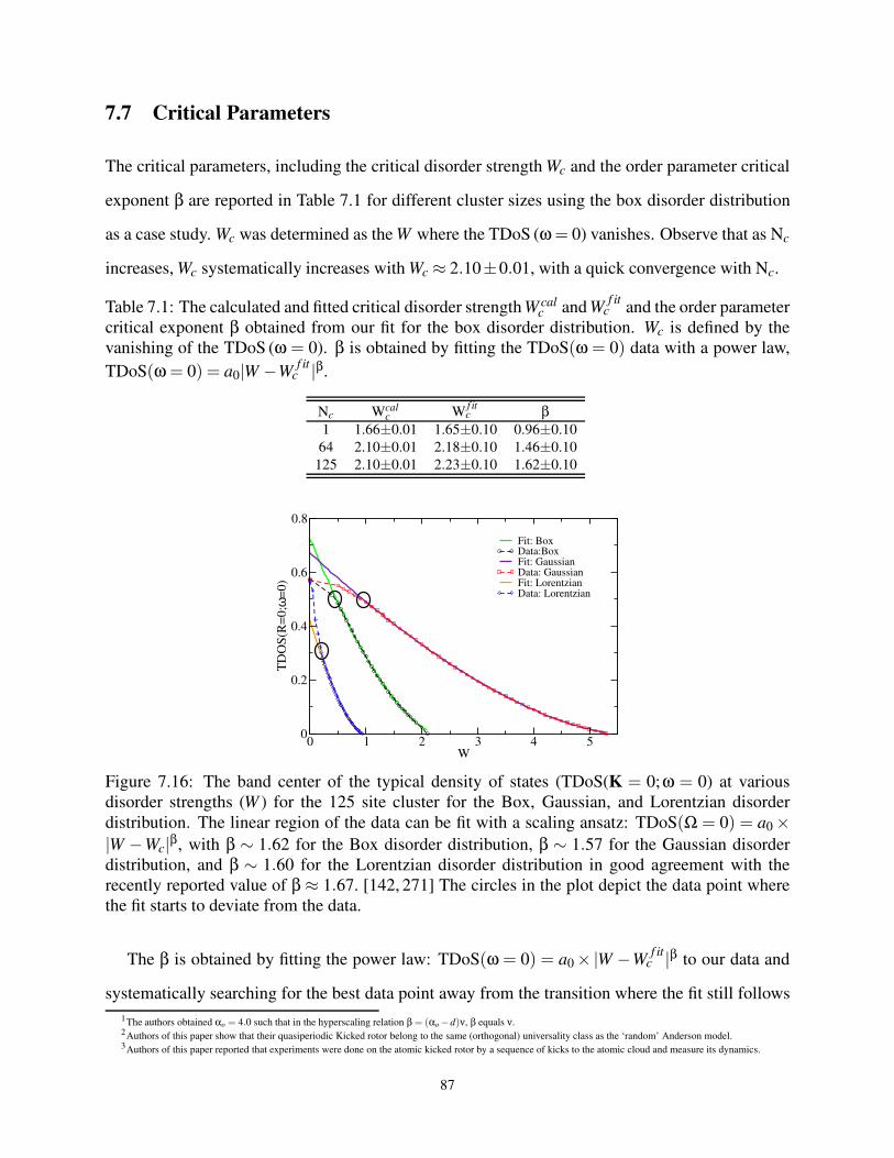
7.7 Critical Parameters
The critical parameters, including the critical disorder strength Wc and the order parameter critical
exponent β are reported in Table 7.1 for different cluster sizes using the box disorder distribution
as a case study. Wc was determined as the W where the TDoS (ω = 0) vanishes. Observe that as Nc
increases, Wc systematically increases with Wc ≈ 2.10±0.01, with a quick convergence with Nc.
Table 7.1: The calculated and fitted critical disorder strength W calc and W
f itc and the order parameter
critical exponent β obtained from our fit for the box disorder distribution. Wc is defined by the
vanishing of the TDoS (ω = 0). β is obtained by fitting the TDoS(ω = 0) data with a power law,
TDoS(ω = 0) = a0|W −Wf it
c |β.
Nc Wcalc W
f itc β
1 1.66±0.01 1.65±0.10 0.96±0.10
64 2.10±0.01 2.18±0.10 1.46±0.10
125 2.10±0.01 2.23±0.10 1.62±0.10
0 1 2 3 4 5W
0
0.2
0.4
0.6
0.8
TD
OS
(R=
0;ω
=0
)
Fit: BoxData:BoxFit: GaussianData: GaussianFit: LorentzianData: Lorentzian
Figure 7.16: The band center of the typical density of states (TDoS(K = 0;ω = 0) at various
disorder strengths (W ) for the 125 site cluster for the Box, Gaussian, and Lorentzian disorder
distribution. The linear region of the data can be fit with a scaling ansatz: TDoS(Ω = 0) = a0 ×|W −Wc|β, with β ∼ 1.62 for the Box disorder distribution, β ∼ 1.57 for the Gaussian disorder
distribution, and β ∼ 1.60 for the Lorentzian disorder distribution in good agreement with the
recently reported value of β ≈ 1.67. [142, 271] The circles in the plot depict the data point where
the fit starts to deviate from the data.
The β is obtained by fitting the power law: TDoS(ω = 0) = a0 ×|W −Wf it
c |β to our data and
systematically searching for the best data point away from the transition where the fit still follows
1The authors obtained αo = 4.0 such that in the hyperscaling relation β = (αo −d)ν, β equals ν.2Authors of this paper show that their quasiperiodic Kicked rotor belong to the same (orthogonal) universality class as the ‘random’ Anderson model.3Authors of this paper reported that experiments were done on the atomic kicked rotor by a sequence of kicks to the atomic cloud and measure its dynamics.
87
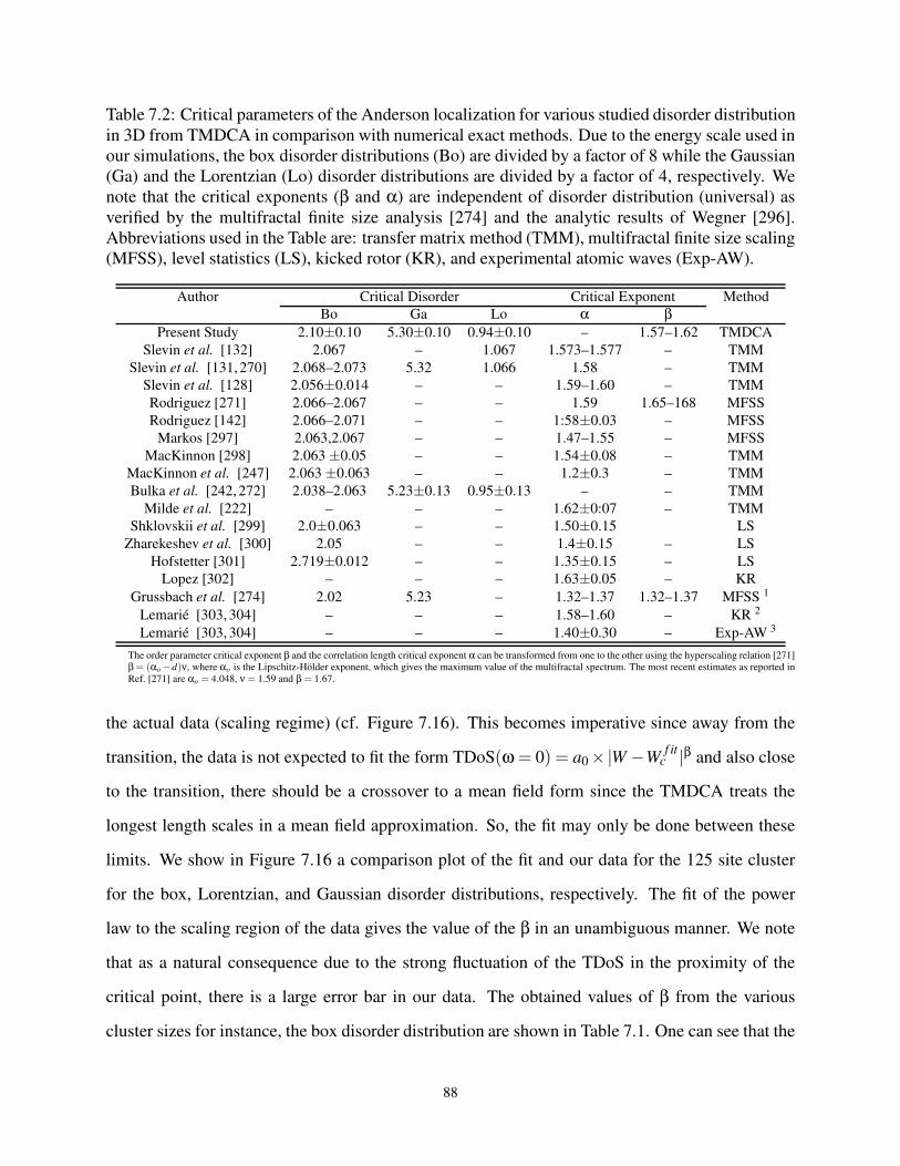
Table 7.2: Critical parameters of the Anderson localization for various studied disorder distribution
in 3D from TMDCA in comparison with numerical exact methods. Due to the energy scale used in
our simulations, the box disorder distributions (Bo) are divided by a factor of 8 while the Gaussian
(Ga) and the Lorentzian (Lo) disorder distributions are divided by a factor of 4, respectively. We
note that the critical exponents (β and α) are independent of disorder distribution (universal) as
verified by the multifractal finite size analysis [274] and the analytic results of Wegner [296].
Abbreviations used in the Table are: transfer matrix method (TMM), multifractal finite size scaling
(MFSS), level statistics (LS), kicked rotor (KR), and experimental atomic waves (Exp-AW).
Author Critical Disorder Critical Exponent Method
Bo Ga Lo α β
Present Study 2.10±0.10 5.30±0.10 0.94±0.10 – 1.57–1.62 TMDCA
Slevin et al. [132] 2.067 – 1.067 1.573–1.577 – TMM
Slevin et al. [131, 270] 2.068–2.073 5.32 1.066 1.58 – TMM
Slevin et al. [128] 2.056±0.014 – – 1.59–1.60 – TMM
Rodriguez [271] 2.066–2.067 – – 1.59 1.65–168 MFSS
Rodriguez [142] 2.066–2.071 – – 1:58±0.03 – MFSS
Markos [297] 2.063,2.067 – – 1.47–1.55 – MFSS
MacKinnon [298] 2.063 ±0.05 – – 1.54±0.08 – TMM
MacKinnon et al. [247] 2.063 ±0.063 – – 1.2±0.3 – TMM
Bulka et al. [242, 272] 2.038–2.063 5.23±0.13 0.95±0.13 – – TMM
Milde et al. [222] – – – 1.62±0:07 – TMM
Shklovskii et al. [299] 2.0±0.063 – – 1.50±0.15 LS
Zharekeshev et al. [300] 2.05 – – 1.4±0.15 – LS
Hofstetter [301] 2.719±0.012 – – 1.35±0.15 – LS
Lopez [302] – – – 1.63±0.05 – KR
Grussbach et al. [274] 2.02 5.23 – 1.32–1.37 1.32–1.37 MFSS 1
Lemarié [303, 304] – – – 1.58–1.60 – KR 2
Lemarié [303, 304] – – – 1.40±0.30 – Exp-AW 3
The order parameter critical exponent β and the correlation length critical exponent α can be transformed from one to the other using the hyperscaling relation [271]
β = (αo −d)ν, where αo is the Lipschitz-Hölder exponent, which gives the maximum value of the multifractal spectrum. The most recent estimates as reported in
Ref. [271] are αo = 4.048, ν = 1.59 and β = 1.67.
the actual data (scaling regime) (cf. Figure 7.16). This becomes imperative since away from the
transition, the data is not expected to fit the form TDoS(ω = 0) = a0 ×|W −Wf it
c |β and also close
to the transition, there should be a crossover to a mean field form since the TMDCA treats the
longest length scales in a mean field approximation. So, the fit may only be done between these
limits. We show in Figure 7.16 a comparison plot of the fit and our data for the 125 site cluster
for the box, Lorentzian, and Gaussian disorder distributions, respectively. The fit of the power
law to the scaling region of the data gives the value of the β in an unambiguous manner. We note
that as a natural consequence due to the strong fluctuation of the TDoS in the proximity of the
critical point, there is a large error bar in our data. The obtained values of β from the various
cluster sizes for instance, the box disorder distribution are shown in Table 7.1. One can see that the
88
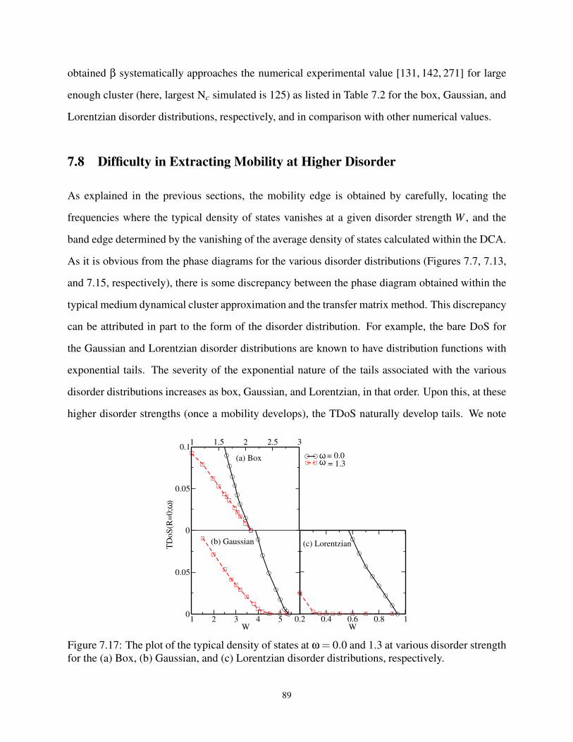
obtained β systematically approaches the numerical experimental value [131, 142, 271] for large
enough cluster (here, largest Nc simulated is 125) as listed in Table 7.2 for the box, Gaussian, and
Lorentzian disorder distributions, respectively, and in comparison with other numerical values.
7.8 Difficulty in Extracting Mobility at Higher Disorder
As explained in the previous sections, the mobility edge is obtained by carefully, locating the
frequencies where the typical density of states vanishes at a given disorder strength W , and the
band edge determined by the vanishing of the average density of states calculated within the DCA.
As it is obvious from the phase diagrams for the various disorder distributions (Figures 7.7, 7.13,
and 7.15, respectively), there is some discrepancy between the phase diagram obtained within the
typical medium dynamical cluster approximation and the transfer matrix method. This discrepancy
can be attributed in part to the form of the disorder distribution. For example, the bare DoS for
the Gaussian and Lorentzian disorder distributions are known to have distribution functions with
exponential tails. The severity of the exponential nature of the tails associated with the various
disorder distributions increases as box, Gaussian, and Lorentzian, in that order. Upon this, at these
higher disorder strengths (once a mobility develops), the TDoS naturally develop tails. We note
1 1.5 2 2.5 3
0
0.05
0.1ωω
0.2 0.4 0.6 0.8 1W
1 2 3 4 5W
0
0.05
(a) Box
(b) Gaussian (c) LorentzianTD
oS
(R=
0;ω
)
= 0.0= 1.3
Figure 7.17: The plot of the typical density of states at ω = 0.0 and 1.3 at various disorder strength
for the (a) Box, (b) Gaussian, and (c) Lorentzian disorder distributions, respectively.
89
that in our computations, aside the initial small broadening value ∼−0.01 used in the initialization
of the self-energy (needed only for the first iteration), no broadening factor is utilized. As such,
these tails that emerge as disorder strength is increased towards Wc are physical tails since the top
and bottom of the bands will localize first. To demonstrate this, we show in Figure 7.17, the plot
of the TDoS at ω = 0.0 and ω = 1.3 (note the ω = 1.3 frequency is arbitrary but chosen in such
a way that it is close to the re-entrance region of the mobility edge) for the box, Gaussian, and
Lorentzian disorder distributions, respectively. As can be seen from the plots, for the box disorder
distribution, even though there are small tails, the TDoS at ω = 0.0 and ω = 1.3 behave alike and
differ only in magnitude. There are no obvious long tails in either frequency (ω = 0.0 and 1.3) that
may mask the detection of the position of the mobility edge energies. However, for the Gaussian
and Lorentzian disorder distributions, there are exponentially very long tails especially at ω = 1.3
that make pinpointing the exact position of the mobility edge energies highly non-trivial. This
should further be understood from the fact that unlike the box disorder distribution, the Lorentzian
disorder distribution naturally has tails that decay very slowly at infinity, as |x|−2, such that aside
the zeroth moment (the area under the curve), all other higher moments do not even exists.
We note that this difficulty is generic not only to the TMDCA but also for any method where
the extraction of the trajectories of the mobility edge is based on the TDoS. A notable example is
in the kernel polynomial method, which even shows more severe discrepancy (not shown).
This deviation between the TMDCA and TMM at higher disorder strengths can also be at-
tributed to the fact that the TMDCA just like the KPM utilizes finite frequency grid (which biases
more towards the metallic regime) in contrast to the TMM, which calculates the transmission of
electrons at fixed energies. Even at this, we note that the TMM also has its own short-comings
around the same regime due to the strong fluctuations in Λ as can be seen in the phase diagrams
for the various disorder strengths around the re-entrance regime.
90
7.9 Conclusions
A detailed study of the Anderson localization transitions using a new formalism: typical medium
dynamical cluster approximation (TMDCA) for various disorder distributions: box, Gaussian,
Lorentzian and alloy models in 3-dimensions have been presented. In all the disorder distribu-
tions studied, the TMDCA is shown to be a successful, self-consistent, preserving causality, and
numerically efficient effective scheme for characterizing disordered electron systems.
With our formalism, we demonstrate that the typical DoS vanishes for localized states and is
finite for states, which are extended. Employing the typical DoS as an order parameter for the An-
derson localization, we have constructed the disorder-energy phase diagram, computed the critical
disorder strengths (Wc), and extracted the order parameter critical exponent (β) for the various dis-
order distributions and benchmark them in good agreement with various numerical exact methods.
We show that β for the Anderson localization transitions is a universal parameter independent of
any disorder distribution in agreement with the multifractal analysis. [274] For distributions with
a finite variance (box and Gaussian), we demonstrate that there are extended states outside the
unperturbed band.
We further show using the DCA (which includes spatial correlations) and a variant of the typical
medium (which includes spatial correlations but suffers from self-averaging), the importance of
the effective medium to properly characterize the Anderson localization transitions. We further
demonstrate the inability of the single site CPA and the TMT methods to accurately capture the
localization and disorder effects in both the average and the typical DoS, respectively. We note
that the single site TMT while being able to quantitatively capture the localization transitions,
strongly underestimates the extended regions with severe underestimation of the critical parameters
including the mobility edge trajectories. In contrast, the TMDCA captures nicely, the trajectories
of the mobility edge with great improvement in the critical parameters. Most importantly, the
TMDCA results are found to be in a quantitative agreement with exact numerical results.
The TMDCA formalism is computationally inexpensive and straightforward to implement since
it requires only the computer time needed to diagonalize small clusters, average over the disor-
91
der configurations, and iterate to convergence. Once combined with electronic structure calcula-
tions [305] and more sophisticated many-body techniques for electron interactions, it will open
a new avenue for studying localization phenomenon in real materials, as well as the competition
between disorder and electron correlations.
Note that a small size cluster is needed to get a converged result in good agreement with the
TMM results. As noted earlier, the TMDCA is highly inexpensive. To show this, we compare
the relative CPU time needed for the largest system size simulated in the TMDCA and the TMM,
respectively. For the largest cluster size utilized in the TMDCA calculations, which is Nc = 216,
the compute-time is ∼ 3-4 hours (running on a single processor) as against ∼ 15-20 hours needed
for each point in the TMM calculations for the system sizes in Figure 7.7.
92
Chapter 8
Application of Typical Medium Dynamical
Cluster Approximation to Off-diagonal
Three Dimensional Disordered SystemThe results presented in this chapter has been published in Phys. Rev. B 90, 094208 (2014) [3].
This is the generalization of the local Blackman, Esterling, and Berk (BEB) method for systems
with the off-diagonal disorder to finite cluster both for the DCA and the TMDCA. The list of the
authors, as it appears in the manuscript are H. Terletska, C. E. Ekuma, C. Moore, K.-M. Tam, J.
Moreno, and M. Jarrell.
8.1 Introduction
Disorder which is inevitably present in most materials can dramatically affect their properties [46,
69]. There have been a number of attempts to develop systematic non-local extensions to the
CPA. These include cluster extensions such as the molecular coherent potential approximation
(MCPA) [306,307], the dynamical cluster approximation (DCA) [263,264,308], etc. Self-consistent
mean field studies of off-diagonal disorder have been conducted by a number of authors [307,309–
311]. However, all these studies have been performed at the local single-site BEB level. To in-
clude the effects of off-diagonal disorder, Gonis [306] extended the Molecular CPA, which uses
a self-consistently embedded finite size cluster to capture non-local corrections to the CPA. How-
ever, he criticized the MCPA for violating translational invariance and other critical properties of
a valid quantum cluster theory [2, 266]. In order to take into account such non-local effects of
off-diagonal disorder models, while maintaining translational invariance, we first extend the BEB
formalism using the DCA scheme [263, 264, 308] and then incorporate typical medium using the
TMDCA [2].
93
While the CPA, DCA, and BEB have been shown to be successful, self-consistent mean-field
theories for the quantitative description of the density of states and electronic structure of disor-
dered systems, they can not properly address the physics of Anderson localization. These mean-
field approaches describe the effective medium using the average density of states which is not
critical at the transition [2, 70, 120, 134, 255, 283]. Thus, theories which rely on such averaged
quantities will fail to properly characterize the Anderson localization. As noted by Anderson, the
probability distribution of the local density of states must be considered, focusing on the most
probable or the typical value [35, 312]. Close to the Anderson transition, the distribution is found
to have very long tails characteristic of a log-normal distribution [138,142,313]. In fact, the distri-
bution is log-normal up to ten orders of magnitude [257] and so the typical value [65,269,313,314]
is the geometrical mean. Based on this idea, Dobrosavljevic et al. [105] formulated a single site
typical medium theory (TMT) for the Anderson localization. This approximation only gives a qual-
itative description of the Anderson localization in three dimensions. However, it fails to properly,
describe critical properties of the localization transitions including the trajectory of the mobility
edge (which separates the extended and localized states), the order parameter critical exponent, and
the critical disorder strengths as it neglects non-local (spatial) correlations and so does not include
the effects of coherent backscattering [315]. In addition, TMT is only formulated for the diagonal
disorder.
In this chapter, to go beyond the local single-site CPA-like level of the BEB formalism, we
employ the DCA [263, 264, 308] scheme which systematically incorporates non-local spatial cor-
relation effects. We first present an extension of the DCA for systems with both diagonal and
off-diagonal disorder. Comparing our single site and finite cluster results, we demonstrate the ef-
fect of non-local correlations on the density of states and the self-energy. A further benchmarking
with numerical exact methods is demonstrated.
Up to now, there exist no typical medium formalism for systems with off-diagonal disorder. So
far, the typical medium analysis has been applied to systems with only diagonal disorder [2, 105].
In this chapter, we develop a typical medium dynamical cluster approximation formalism capa-
ble of characterizing the localization transition in systems with both diagonal and off-diagonal
94

disorder. We perform a systematic study of the effects of non-local correlations and off-diagonal
randomness on the density of states and the electron localization. By comparing the single site and
finite cluster results for the typical density of states, we demonstrate the importance of incorporat-
ing the non-local, multi-sites effects for proper and quantitative characterization of the localization
transition. The results of our calculations are compared with the ones obtained with other numeri-
cal methods for finite size lattices, including exact diagonalization, kernel polynomial, and transfer
matrix methods.
8.2 Formalism
The formalism that will be generalized here is already presented in Chapter 5 and will not be
repeated here. I will next present the extension of the DCA and the TMDCA for the study of
systems with both diagonal and non-diagonal randomness.
8.2.1 Dynamical Cluster Approximation for Off-diagonal Disorder
The simplest model widely used to study disordered systems is the single band, tight binding
Hamiltonian defined by Equation 4.1. Here, the probability distribution is defined by Equa-
tion 4.2d. For the diagonal disorder case when the bandwidth of the pure host A is about the
same that the bandwidth of the B system, such substitution results only in a change of the local
potential Vi at the replaced site i. This corresponds to changes only in the diagonal elements of the
Hamiltonian. In this case, it is assumed that the substitution of impurity atoms on average has no
effect on the hopping amplitudes to the neighboring atomic sites.
For systems with off-diagonal disorder, the randomness is introduced not only locally in the
random diagonal potential Vi, but also through the hopping amplitudes. To model this, BEB [316]
introduced the disorder configuration dependent hopping amplitude of electrons ti j as
95
ti j = tAAi j , if i ∈ A, j ∈ A
tBBi j , if i ∈ B, j ∈ B
tABi j , if i ∈ A, j ∈ B
tBAi j , if i ∈ B, j ∈ A, (8.1)
where ti j depends on the type of ion occupying sites i and j. For off-diagonal disorder BEB [316]
demonstrated that the scalar CPA equation becomes a 2× 2 matrix equation, with corresponding
AA, AB, BA, and BB matrix elements. In momentum space, if there is only near-neighbor hopping
between all ions, the bare dispersion can be written as (the under-bar denotes matrices)
εk =
tAA tAB
tBA tBB
εk, where εk =−2t ∑di=1 cos(kia) (8.2)
is the dispersion, a is the lattice constant (a= 1), d is the dimension and for d = 3, εk =−2t(cos(kx)+
cos(ky)+ cos(kz)) with 4t = 1 as our unit of energy. tAA, tBB, tAB, and tBA are unitless prefactors.
The BEB approach by construction is local, as such, all nonlocal disorder induced correlations
are neglected [316]. In order to take into account nonlocal physics, we extend the BEB formalism
to a finite cluster using the DCA scheme. Here in the following, we present the algorithm and
details of our nonlocal DCA extension of the BEB formalism for the off-diagonal disorder. Just as
in the DCA scheme [264], the first Brillouin zone is divided into Nc = Ld (d is the dimension and L
is the linear cluster size) coarse-grained cells with centers K surrounded by points k within the cell
so that an arbitrary k = K+ k. For a given DCA, the K-dependent effective medium hybridization
Γ(K,ω) matrix in momentum space is
Γ(K,ω) =
ΓAA(K,ω) ΓAB(K,ω)
ΓBA(K,ω) ΓBB(K,ω)
(8.3)
96
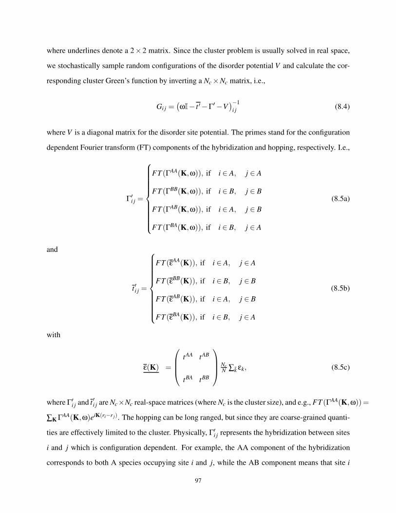
where underlines denote a 2×2 matrix. Since the cluster problem is usually solved in real space,
we stochastically sample random configurations of the disorder potential V and calculate the cor-
responding cluster Green’s function by inverting a Nc ×Nc matrix, i.e.,
Gi j =(ωI− t ′−Γ′−V
)−1
i j(8.4)
where V is a diagonal matrix for the disorder site potential. The primes stand for the configuration
dependent Fourier transform (FT) components of the hybridization and hopping, respectively. I.e.,
Γ′i j =
FT (ΓAA(K,ω)), if i ∈ A, j ∈ A
FT (ΓBB(K,ω)), if i ∈ B, j ∈ B
FT (ΓAB(K,ω)), if i ∈ A, j ∈ B
FT (ΓBA(K,ω)), if i ∈ B, j ∈ A
(8.5a)
and
t′i j =
FT (εAA(K)), if i ∈ A, j ∈ A
FT (εBB(K)), if i ∈ B, j ∈ B
FT (εAB(K)), if i ∈ A, j ∈ B
FT (εBA(K)), if i ∈ B, j ∈ A
(8.5b)
with
ε(K) =
tAA tAB
tBA tBB
Nc
N ∑k εk, (8.5c)
where Γ′i j and t
′i j are Nc×Nc real-space matrices (where Nc is the cluster size), and e.g., FT (ΓAA(K,ω))=
∑K ΓAA(K,ω)eiK(ri−r j). The hopping can be long ranged, but since they are coarse-grained quanti-
ties are effectively limited to the cluster. Physically, Γ′i j represents the hybridization between sites
i and j which is configuration dependent. For example, the AA component of the hybridization
corresponds to both A species occupying site i and j, while the AB component means that site i
97

is occupied by an A atom and site j by a B atom. The interpretation of the hopping matrix is the
same as for the hybridization function.
In the next step, we perform averaging over the disorder 〈(...)〉 and in doing so we re-expand
the Green function (Equation 8.4) into a 2Nc ×2Nc matrix
Gc(ω)i j =
⟨GAA
c (ω)⟩
i j
⟨GAB
c (ω)⟩
i j
⟨GBA
c (ω)⟩
i j
⟨GBB
c (ω)⟩
i j
. (8.6)
This may be done by assigning the components according to the occupancy of the sites i and j
(GAAc )i j = (Gc)i j if i ∈ A, j ∈ A
(GBBc )i j = (Gc)i j if i ∈ B, j ∈ B
(GABc )i j = (Gc)i j if i ∈ A, j ∈ B
(GBAc )i j = (Gc)i j if i ∈ B, j ∈ A (8.7)
with the other components being zero. Because only one of the four matrix elements is finite for
each disorder configuration (each site can be occupied by either A or B atom), only the sum of the
elements in Equation 8.6 is normalized as a conventional Green function.
Having formed the disorder average cluster Green function matrix, we then Fourier transform
each component to K-space (which also imposes translational symmetry) and construct the K-
dependent disorder averaged cluster Green function matrix in momentum space
Gc(K,ω) =
GAAc (K,ω) GAB
c (K,ω)
GBAc (K,ω) GBB
c (K,ω)
. (8.8)
98
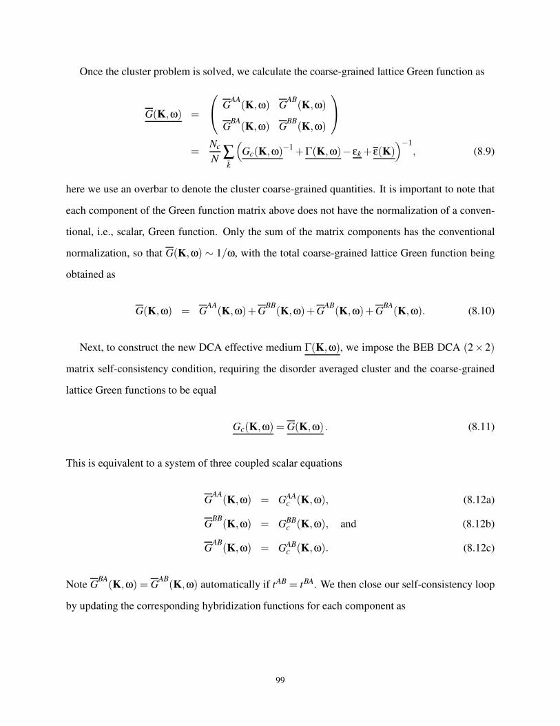
Once the cluster problem is solved, we calculate the coarse-grained lattice Green function as
G(K,ω) =
G
AA(K,ω) G
AB(K,ω)
GBA(K,ω) G
BB(K,ω)
=Nc
N∑k
(
Gc(K,ω)−1 +Γ(K,ω)− εk + ε(K))−1
, (8.9)
here we use an overbar to denote the cluster coarse-grained quantities. It is important to note that
each component of the Green function matrix above does not have the normalization of a conven-
tional, i.e., scalar, Green function. Only the sum of the matrix components has the conventional
normalization, so that G(K,ω) ∼ 1/ω, with the total coarse-grained lattice Green function being
obtained as
G(K,ω) = GAA(K,ω)+G
BB(K,ω)+G
AB(K,ω)+G
BA(K,ω). (8.10)
Next, to construct the new DCA effective medium Γ(K,ω), we impose the BEB DCA (2×2)
matrix self-consistency condition, requiring the disorder averaged cluster and the coarse-grained
lattice Green functions to be equal
Gc(K,ω) = G(K,ω) . (8.11)
This is equivalent to a system of three coupled scalar equations
GAA(K,ω) = GAA
c (K,ω), (8.12a)
GBB(K,ω) = GBB
c (K,ω), and (8.12b)
GAB(K,ω) = GAB
c (K,ω). (8.12c)
Note GBA(K,ω) = G
AB(K,ω) automatically if tAB = tBA. We then close our self-consistency loop
by updating the corresponding hybridization functions for each component as
99
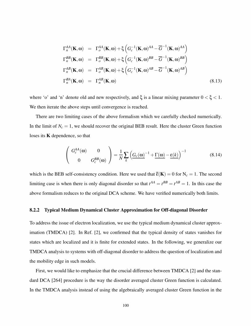
ΓAAn (K,ω) = ΓAA
o (K,ω)+ξ(
G−1c (K,ω)AA−G
−1(K,ω)AA
)
ΓBBn (K,ω) = ΓBB
o (K,ω)+ξ(
G−1c (K,ω)BB−G
−1(K,ω)BB
)
ΓABn (K,ω) = ΓAB
o (K,ω)+ξ(
G−1c (K,ω)AB−G
−1(K,ω)AB
)
ΓBAn (K,ω) = ΓAB
n (K,ω) (8.13)
where ‘o’ and ‘n’ denote old and new respectively, and ξ is a linear mixing parameter 0 < ξ < 1.
We then iterate the above steps until convergence is reached.
There are two limiting cases of the above formalism which we carefully checked numerically.
In the limit of Nc = 1, we should recover the original BEB result. Here the cluster Green function
loses its K dependence, so that
GAA
c (ω) 0
0 GBBc (ω)
=1
N∑k
(
Gc(ω)−1 +Γ(ω)− ε(k)
)−1
(8.14)
which is the BEB self-consistency condition. Here we used that ε(K) = 0 for Nc = 1. The second
limiting case is when there is only diagonal disorder so that tAA = tBB = tAB = 1. In this case the
above formalism reduces to the original DCA scheme. We have verified numerically both limits.
8.2.2 Typical Medium Dynamical Cluster Approximation for Off-diagonal Disorder
To address the issue of electron localization, we use the typical medium dynamical cluster approx-
imation (TMDCA) [2]. In Ref. [2], we confirmed that the typical density of states vanishes for
states which are localized and it is finite for extended states. In the following, we generalize our
TMDCA analysis to systems with off-diagonal disorder to address the question of localization and
the mobility edge in such models.
First, we would like to emphasize that the crucial difference between TMDCA [2] and the stan-
dard DCA [264] procedure is the way the disorder averaged cluster Green function is calculated.
In the TMDCA analysis instead of using the algebraically averaged cluster Green function in the
100
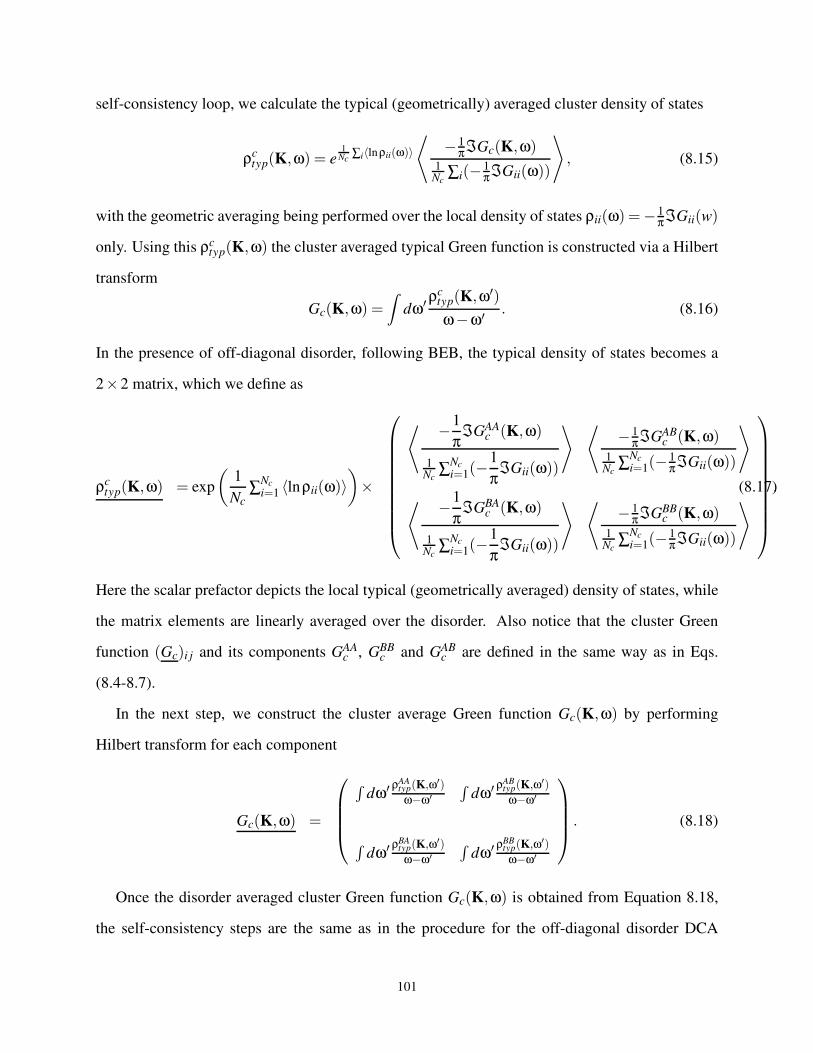
self-consistency loop, we calculate the typical (geometrically) averaged cluster density of states
ρctyp(K,ω) = e
1Nc
∑i〈lnρii(ω)〉⟨
− 1πℑGc(K,ω)
1Nc
∑i(− 1πℑGii(ω))
⟩
, (8.15)
with the geometric averaging being performed over the local density of states ρii(ω) =− 1πℑGii(w)
only. Using this ρctyp(K,ω) the cluster averaged typical Green function is constructed via a Hilbert
transform
Gc(K,ω) =∫
dω′ρctyp(K,ω′)
ω−ω′ . (8.16)
In the presence of off-diagonal disorder, following BEB, the typical density of states becomes a
2×2 matrix, which we define as
ρctyp(K,ω) = exp
(1
Nc∑
Nc
i=1 〈lnρii(ω)〉)
×
⟨ −1
πℑGAA
c (K,ω)
1Nc
∑Nc
i=1(−1
πℑGii(ω))
⟩ ⟨
− 1πℑGAB
c (K,ω)1
Nc∑
Nc
i=1(− 1πℑGii(ω))
⟩
⟨ −1
πℑGBA
c (K,ω)
1Nc
∑Nc
i=1(−1
πℑGii(ω))
⟩ ⟨
− 1πℑGBB
c (K,ω)1
Nc∑
Nc
i=1(− 1πℑGii(ω))
⟩
.(8.17)
Here the scalar prefactor depicts the local typical (geometrically averaged) density of states, while
the matrix elements are linearly averaged over the disorder. Also notice that the cluster Green
function (Gc)i j and its components GAAc , GBB
c and GABc are defined in the same way as in Eqs.
(8.4-8.7).
In the next step, we construct the cluster average Green function Gc(K,ω) by performing
Hilbert transform for each component
Gc(K,ω) =
∫dω′ ρAA
typ(K,ω′)ω−ω′
∫dω′ ρAB
typ(K,ω′)ω−ω′
∫dω′ ρBA
typ(K,ω′)ω−ω′
∫dω′ ρBB
typ(K,ω′)ω−ω′
. (8.18)
Once the disorder averaged cluster Green function Gc(K,ω) is obtained from Equation 8.18,
the self-consistency steps are the same as in the procedure for the off-diagonal disorder DCA
101
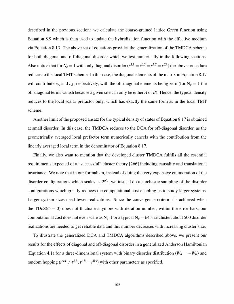
described in the previous section: we calculate the coarse-grained lattice Green function using
Equation 8.9 which is then used to update the hybridization function with the effective medium
via Equation 8.13. The above set of equations provides the generalization of the TMDCA scheme
for both diagonal and off-diagonal disorder which we test numerically in the following sections.
Also notice that for Nc = 1 with only diagonal disorder (tAA = tBB = tAB = tBA) the above procedure
reduces to the local TMT scheme. In this case, the diagonal elements of the matrix in Equation 8.17
will contribute cA and cB, respectively, with the off-diagonal elements being zero (for Nc = 1 the
off-diagonal terms vanish because a given site can only be either A or B). Hence, the typical density
reduces to the local scalar prefactor only, which has exactly the same form as in the local TMT
scheme.
Another limit of the proposed ansatz for the typical density of states of Equation 8.17 is obtained
at small disorder. In this case, the TMDCA reduces to the DCA for off-diagonal disorder, as the
geometrically averaged local prefactor term numerically cancels with the contribution from the
linearly averaged local term in the denominator of Equation 8.17.
Finally, we also want to mention that the developed cluster TMDCA fulfills all the essential
requirements expected of a “successful” cluster theory [266] including causality and translational
invariance. We note that in our formalism, instead of doing the very expensive enumeration of the
disorder configurations which scales as 2Nc, we instead do a stochastic sampling of the disorder
configurations which greatly reduces the computational cost enabling us to study larger systems.
Larger system sizes need fewer realizations. Since the convergence criterion is achieved when
the TDoS(ω = 0) does not fluctuate anymore with iteration number, within the error bars, our
computational cost does not even scale as Nc. For a typical Nc = 64 size cluster, about 500 disorder
realizations are needed to get reliable data and this number decreases with increasing cluster size.
To illustrate the generalized DCA and TMDCA algorithms described above, we present our
results for the effects of diagonal and off-diagonal disorder in a generalized Anderson Hamiltonian
(Equation 4.1) for a three-dimensional system with binary disorder distribution (WA = −WB) and
random hopping (tAA 6= tBB, tAB = tBA) with other parameters as specified.
102
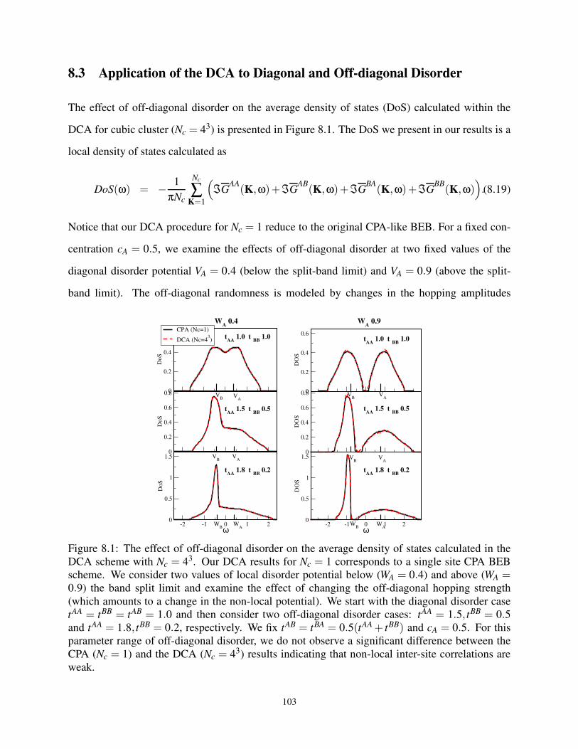
8.3 Application of the DCA to Diagonal and Off-diagonal Disorder
The effect of off-diagonal disorder on the average density of states (DoS) calculated within the
DCA for cubic cluster (Nc = 43) is presented in Figure 8.1. The DoS we present in our results is a
local density of states calculated as
DoS(ω) = − 1
πNc
Nc
∑K=1
(
ℑGAA(K,ω)+ℑG
AB(K,ω)+ℑG
BA(K,ω)+ℑG
BB(K,ω)
)
.(8.19)
Notice that our DCA procedure for Nc = 1 reduce to the original CPA-like BEB. For a fixed con-
centration cA = 0.5, we examine the effects of off-diagonal disorder at two fixed values of the
diagonal disorder potential VA = 0.4 (below the split-band limit) and VA = 0.9 (above the split-
band limit). The off-diagonal randomness is modeled by changes in the hopping amplitudes
-2 -1 0 1 2ω
0
0.5
1
1.5
Do
S
-2 -1 0 1 2ω
0
0.5
1
1.5
DO
S
0
0.2
0.4
0.6
0.8
Do
S
0
0.2
0.4
0.6
Do
S
CPA (Nc=1)
DCA (Nc=43)
0
0.2
0.4
0.6
0.8
DO
S
0
0.2
0.4
0.6
DO
S
tAA
=1.0, tBB
=1.0
tAA
=1.5, tBB
=0.5
tAA
=1.8, tBB
=0.2
WA
=0.4
VA
VB
VA
WA
WB
VB
tAA
=1.8, tBB
=0.2
WA
=0.9
tAA
=1.5, tBB
=0.5
tAA
=1.0, tBB
=1.0
WA
WB
VA
VB
VA
VB
Figure 8.1: The effect of off-diagonal disorder on the average density of states calculated in the
DCA scheme with Nc = 43. Our DCA results for Nc = 1 corresponds to a single site CPA BEB
scheme. We consider two values of local disorder potential below (WA = 0.4) and above (WA =0.9) the band split limit and examine the effect of changing the off-diagonal hopping strength
(which amounts to a change in the non-local potential). We start with the diagonal disorder case
tAA = tBB = tAB = 1.0 and then consider two off-diagonal disorder cases: tAA = 1.5, tBB = 0.5and tAA = 1.8, tBB = 0.2, respectively. We fix tAB = tBA = 0.5(tAA + tBB) and cA = 0.5. For this
parameter range of off-diagonal disorder, we do not observe a significant difference between the
CPA (Nc = 1) and the DCA (Nc = 43) results indicating that non-local inter-site correlations are
weak.
103
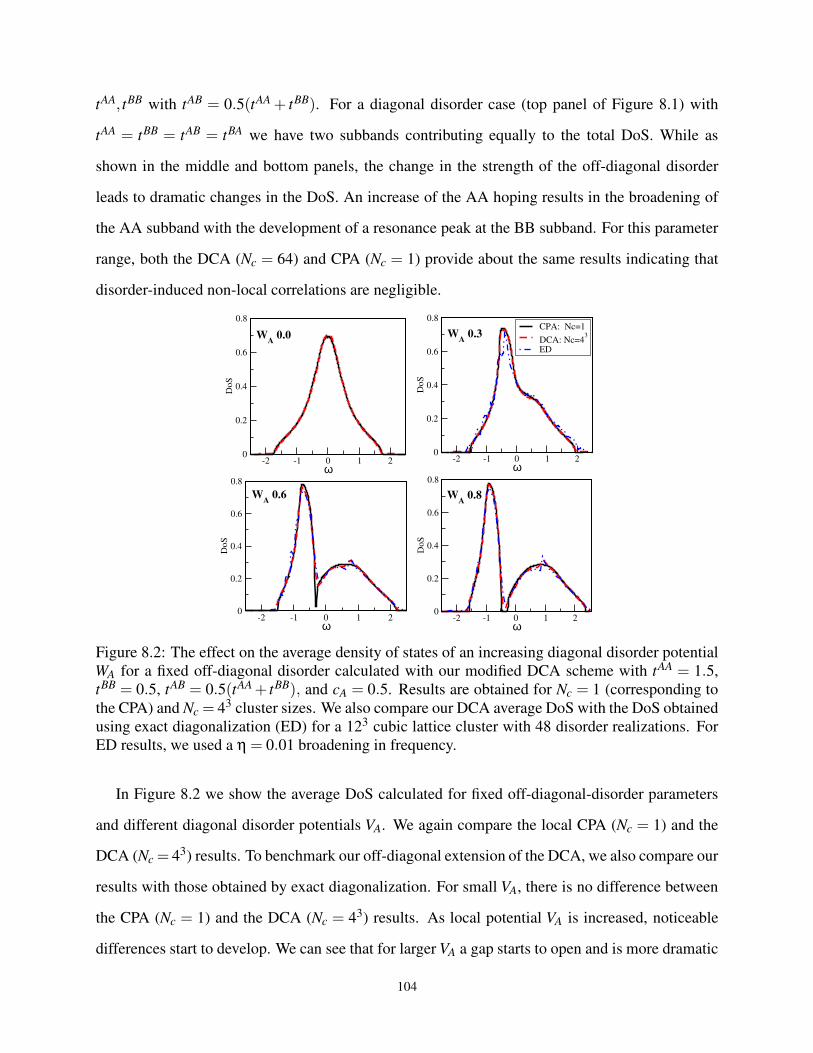
tAA, tBB with tAB = 0.5(tAA + tBB). For a diagonal disorder case (top panel of Figure 8.1) with
tAA = tBB = tAB = tBA we have two subbands contributing equally to the total DoS. While as
shown in the middle and bottom panels, the change in the strength of the off-diagonal disorder
leads to dramatic changes in the DoS. An increase of the AA hoping results in the broadening of
the AA subband with the development of a resonance peak at the BB subband. For this parameter
range, both the DCA (Nc = 64) and CPA (Nc = 1) provide about the same results indicating that
disorder-induced non-local correlations are negligible.
-2 -1 0 1 2ω
0
0.2
0.4
0.6
0.8
DoS
-2 -1 0 1 2ω
0
0.2
0.4
0.6
0.8
DoS
-2 -1 0 1 2ω
0
0.2
0.4
0.6
0.8
DoS
-2 -1 0 1 2ω
0
0.2
0.4
0.6
0.8
DoS
CPA: Nc=1
DCA: Nc=43
ED
WA
=0.3
WA
=0.6 WA
=0.8
WA
=0.0
Figure 8.2: The effect on the average density of states of an increasing diagonal disorder potential
WA for a fixed off-diagonal disorder calculated with our modified DCA scheme with tAA = 1.5,
tBB = 0.5, tAB = 0.5(tAA+ tBB), and cA = 0.5. Results are obtained for Nc = 1 (corresponding to
the CPA) and Nc = 43 cluster sizes. We also compare our DCA average DoS with the DoS obtained
using exact diagonalization (ED) for a 123 cubic lattice cluster with 48 disorder realizations. For
ED results, we used a η = 0.01 broadening in frequency.
In Figure 8.2 we show the average DoS calculated for fixed off-diagonal-disorder parameters
and different diagonal disorder potentials VA. We again compare the local CPA (Nc = 1) and the
DCA (Nc = 43) results. To benchmark our off-diagonal extension of the DCA, we also compare our
results with those obtained by exact diagonalization. For small VA, there is no difference between
the CPA (Nc = 1) and the DCA (Nc = 43) results. As local potential VA is increased, noticeable
differences start to develop. We can see that for larger VA a gap starts to open and is more dramatic
104
in the CPA scheme. While in the DCA (Nc = 43) this gap is partially filled due to the incorporation
of non-local inter-site correlations which are missing in the CPA. Furthermore, the DoS obtained
from the DCA procedure provides finer structures which are in basic agreement with the DoS
calculated with exact diagonalization for a cluster of size 12×12×12. The agreement we get with
ED results is a good indication of the accuracy of our extension of the DCA to the off-diagonal
disorder. The additional structures observed in the DoS for Nc > 1, which are absent in the CPA, are
believed to be related to the local order in the environment of each site [264,266]. Notice that while
the DCA accounts for non-local backscattering effects which lead to the Anderson localization, the
average local DoS does not capture the transition, as it is not an order parameter for the Anderson
localization.
To further illustrate the important effect of the non-local contributions from the cluster, we also
-2 -1 0 1 2ω
-0.8
-0.6
-0.4
-0.2
-2 -1 0 1 2ω
-0.3
-0.2
-0.1
-2 -1 0 1 2ω
0
0.2
0.4
-2 -1 0 1 2ω
-0.3
-0.2
-0.1
-2 -1 0 1 2ω
0
0.2
0.4
-2 -1 0 1 2ω
-0.8
-0.6
-0.4
-0.2
0
WA
=0.6
WA
=0.1
00
ℑΣAA
(K,ω) ℑΣBB
(K,ω) ℑΣAB
(K,ω)
ℑΣAB
(K,ω)ℑΣBB
(K,ω)ℑΣAA
(K,ω)
0
Figure 8.3: The imaginary part of the self-energy vs frequency ω for Nc = 1 (red dash-line) and
Nc = 43 (solid lines) at various K momenta points: (0,0,0), (π,0,0), (π,π,0), and (π/2,π/2,π/2),for WA = 0.1 (top) and WA = 0.6 (bottom) diagonal disorder potential with tAA = 1.5, tBB = 0.5,
tAB = 0.5(tAA + tBB), and cA = 0.5. For small disorder WA = 0.1, the self-energy for Nc = 1 is
essentially the same as that of the various K points of the Nc = 43 cluster, indicating that non-local
effects are negligible for such small disorder. For a larger value of the disorder WA = 0.6, the
single site and the finite cluster data differ significantly, which illustrates that at larger disorder, the
momentum dependence of the self-energy increases and becomes important.
105
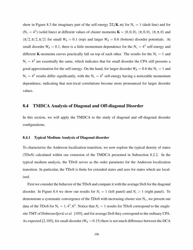
show in Figure 8.3 the imaginary part of the self-energy ℑΣ(K,ω) for Nc = 1 (dash line) and for
(Nc = 43) (solid lines) at different values of cluster momenta K = (0,0,0), (π,0,0), (π,π,0) and
(π/2,π/2,π/2) for small WA = 0.1 (top) and larger WA = 0.6 (bottom) disorder potentials. At
small disorder WA = 0.1, there is a little momentum dependence for the Nc = 43 self-energy and
different K-momenta curves practically fall on top of each other. The results for the Nc = 1 and
Nc = 43 are essentially the same, which indicates that for small disorder the CPA still presents a
good approximation for the self-energy. On the hand, for larger disorder WA = 0.6 the Nc = 1 and
Nc = 43 results differ significantly, with the Nc = 43 self-energy having a noticeable momentum
dependence, indicating that non-local correlations become more pronounced for larger disorder
values.
8.4 TMDCA Analysis of Diagonal and Off-diagonal Disorder
In this section, we will apply the TMDCA to the study of diagonal and off-diagonal disorder
configurations.
8.4.1 Typical Medium Analysis of Diagonal disorder
To characterize the Anderson localization transition, we now explore the typical density of states
(TDoS) calculated within our extension of the TMDCA presented in Subsection 8.2.2. In the
typical medium analysis, the TDoS serves as the order parameter for the Anderson localization
transition. In particular, the TDoS is finite for extended states and zero for states which are local-
ized.
First we consider the behavior of the TDoS and compare it with the average DoS for the diagonal
disorder. In Figure 8.4 we show our results for Nc = 1 (left panel) and Nc > 1 (right panel). To
demonstrate a systematic convergence of the TDoS with increasing cluster size Nc, we present our
data of the TDoS for Nc = 1,43,63. Notice that Nc = 1 results for TDoS correspond to the single-
site TMT of Dobrosavljevic et al. [105], and for average DoS they correspond to the ordinary CPA.
As expected [2,105], for small disorder (WA = 0.15) there is not much difference between the DCA
106
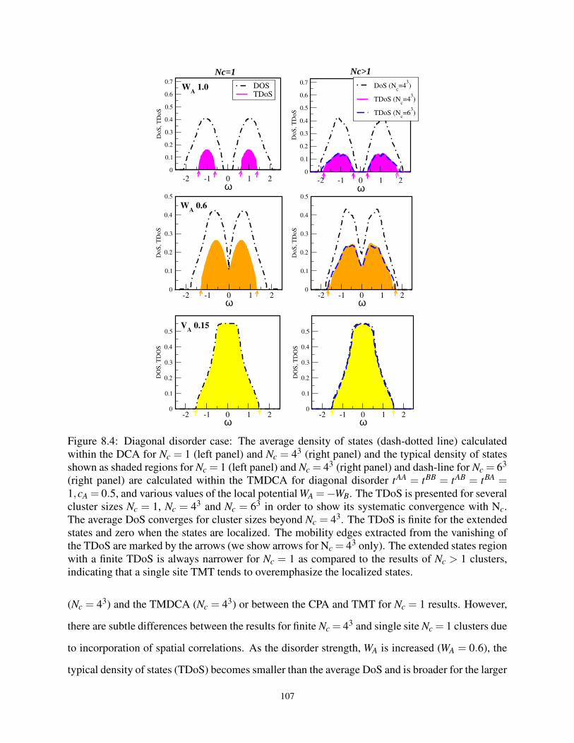
-2 -1 0 1 2ω
0
0.1
0.2
0.3
0.4
0.5
DO
S, T
DO
S-2 -1 0 1 2
ω0
0.1
0.2
0.3
0.4
0.5
DoS
, T
DoS
-2 -1 0 1 2ω
0
0.1
0.2
0.3
0.4
0.5
0.6
0.7
DoS
, T
DoS
DoS (Nc=4
3)
TDoS (Nc=4
3)
TDoS (Nc=6
3)
-2 -1 0 1 2ω
0
0.1
0.2
0.3
0.4
0.5
0.6
0.7
DoS
, T
DoS
DOSTDoS
-2 -1 0 1 2ω
0
0.1
0.2
0.3
0.4
0.5
DoS
, T
DoS
-2 -1 0 1 2ω
0
0.1
0.2
0.3
0.4
0.5
DO
S, T
DO
S
WA
=1.0
WA
=0.6
VA
=0.15
Nc>1Nc=1
Figure 8.4: Diagonal disorder case: The average density of states (dash-dotted line) calculated
within the DCA for Nc = 1 (left panel) and Nc = 43 (right panel) and the typical density of states
shown as shaded regions for Nc = 1 (left panel) and Nc = 43 (right panel) and dash-line for Nc = 63
(right panel) are calculated within the TMDCA for diagonal disorder tAA = tBB = tAB = tBA =1,cA = 0.5, and various values of the local potential WA =−WB. The TDoS is presented for several
cluster sizes Nc = 1, Nc = 43 and Nc = 63 in order to show its systematic convergence with Nc.
The average DoS converges for cluster sizes beyond Nc = 43. The TDoS is finite for the extended
states and zero when the states are localized. The mobility edges extracted from the vanishing of
the TDoS are marked by the arrows (we show arrows for Nc = 43 only). The extended states region
with a finite TDoS is always narrower for Nc = 1 as compared to the results of Nc > 1 clusters,
indicating that a single site TMT tends to overemphasize the localized states.
(Nc = 43) and the TMDCA (Nc = 43) or between the CPA and TMT for Nc = 1 results. However,
there are subtle differences between the results for finite Nc = 43 and single site Nc = 1 clusters due
to incorporation of spatial correlations. As the disorder strength, WA is increased (WA = 0.6), the
typical density of states (TDoS) becomes smaller than the average DoS and is broader for the larger
107
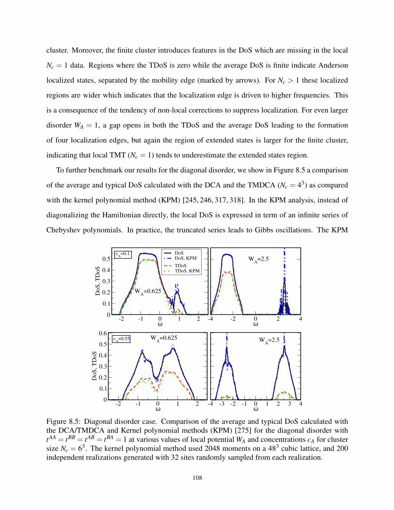
cluster. Moreover, the finite cluster introduces features in the DoS which are missing in the local
Nc = 1 data. Regions where the TDoS is zero while the average DoS is finite indicate Anderson
localized states, separated by the mobility edge (marked by arrows). For Nc > 1 these localized
regions are wider which indicates that the localization edge is driven to higher frequencies. This
is a consequence of the tendency of non-local corrections to suppress localization. For even larger
disorder WA = 1, a gap opens in both the TDoS and the average DoS leading to the formation
of four localization edges, but again the region of extended states is larger for the finite cluster,
indicating that local TMT (Nc = 1) tends to underestimate the extended states region.
To further benchmark our results for the diagonal disorder, we show in Figure 8.5 a comparison
of the average and typical DoS calculated with the DCA and the TMDCA (Nc = 43) as compared
with the kernel polynomial method (KPM) [245, 246, 317, 318]. In the KPM analysis, instead of
diagonalizing the Hamiltonian directly, the local DoS is expressed in term of an infinite series of
Chebyshev polynomials. In practice, the truncated series leads to Gibbs oscillations. The KPM
-2 -1 0 1 2ω
0
0.1
0.2
0.3
0.4
0.5
DoS
, T
DoS
DoS DoS, KPM
TDoS TDoS, KPM
-4 -2 0 2 4ω
-2 -1 0 1 2ω
0
0.1
0.2
0.3
0.4
0.5
0.6
DoS
, T
DoS
-4 -3 -2 -1 0 1 2 3 4ω
cA
=0.1
WA
=2.5
cA
=0.55 WA
=2.5
WA
=0.625
WA
=0.625
Figure 8.5: Diagonal disorder case. Comparison of the average and typical DoS calculated with
the DCA/TMDCA and Kernel polynomial methods (KPM) [275] for the diagonal disorder with
tAA = tBB = tAB = tBA = 1 at various values of local potential WA and concentrations cA for cluster
size Nc = 63. The kernel polynomial method used 2048 moments on a 483 cubic lattice, and 200
independent realizations generated with 32 sites randomly sampled from each realization.
108
damps these oscillations by a modification of the expansion coefficients. Following previous stud-
ies on the Anderson model, the Jackson kernel is used [245]. The details of the implementation are
well discussed in Ref. [245]. The parameters used in the KPM calculations are listed in the caption
of Figure 8.5. As it is evident from the plots, our TMDCA results reproduced those from the KPM
nicely showing that our formalism offers a systematic way of studying the Anderson localization
transition in binary alloy systems. Such good agreement indicates a successful benchmarking of
the TMDCA method [2].
8.4.2 Typical Medium Analysis of Off-diagonal Disorder
Next, we explore the effects of the off-diagonal disorder. In Figure 8.6, we compare the typical
TDoS from the TMDCA and average DoS from the DCA for several values of the diagonal disorder
strength WA at fixed off-diagonal disorder amplitudes tAA = 1.5, tBB = 0.5, tAB = 1.0. To show the
effect of a finite cluster with respect to incorporation of non-local correlations, we present data for
the single site Nc = 1 and finite clusters Nc = 43 and 53. The TMT (Nc = 1) again underestimates the
extended states regime by having a narrower TDoS as compared to the Nc > 1. We also see that the
mobility edge defined by the vanishing of the TDoS (marked by arrows for Nc = 43) systematically
converges with increasing cluster size Nc. For small disorder VA, both the DoS and the TDoS are
practically the same. However, as VA increases, significant differences start to emerge. Increasing
WA leads to the gradual opening of the gap which is more pronounced in the Nc = 1 case and for
smaller disorder VA = 0.6 is partially filled for the Nc > 1 clusters. As compared to the diagonal
disorder case (cf. Figure 8.4), the average DoS and TDoS become asymmetric with respect to zero
frequency due to the off-diagonal randomness.
In Figures 8.7 and 8.8, we present the disorder-energy phase diagram for both diagonal (Fig-
ure 8.7) and off-diagonal (Figure 8.8) disorder calculated using the single TMT (Nc = 1) and the
non-local TMDCA (Nc > 1). To check the accuracy of the mobility edge trajectories extracted
from TMDCA, we compare our data with those obtained with the transfer matrix method (TMM).
The TMM [106,250,251] is a well-established numerical method for calculating the correlation
length and determining the mobility edge of the disorder Anderson model. Its main advantage is
109
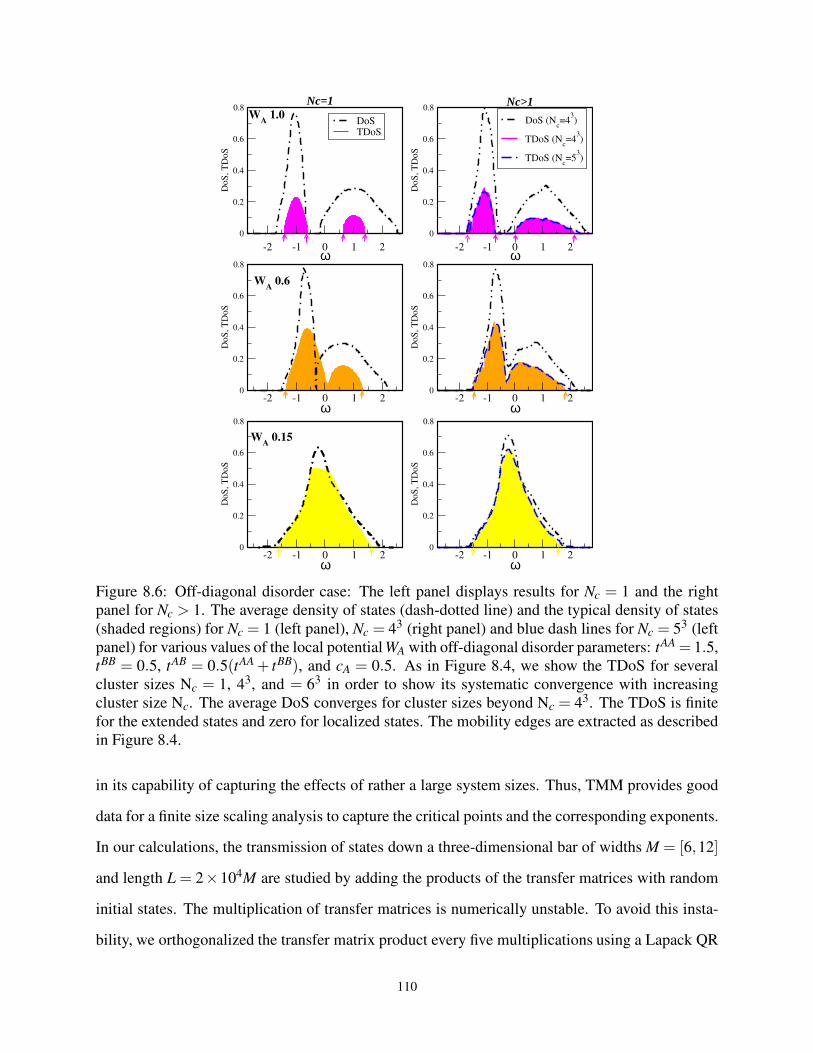
-2 -1 0 1 2ω
0
0.2
0.4
0.6
0.8D
oS
, T
DoS
-2 -1 0 1 2ω
0
0.2
0.4
0.6
0.8
DoS
, T
DoS
-2 -1 0 1 2ω
0
0.2
0.4
0.6
0.8
DoS
, T
DoS
DoS (Nc=4
3)
TDoS (Nc=4
3)
TDoS (Nc=5
3)
-2 -1 0 1 2ω
0
0.2
0.4
0.6
0.8
DoS
, T
DoS
DoSTDoS
-2 -1 0 1 2ω
0
0.2
0.4
0.6
0.8
DoS
, T
DoS
-2 -1 0 1 2ω
0
0.2
0.4
0.6
0.8
DoS
, T
DoS
Nc=1W
A=1.0
WA
=0.6
WA
=0.15
Nc>1
Figure 8.6: Off-diagonal disorder case: The left panel displays results for Nc = 1 and the right
panel for Nc > 1. The average density of states (dash-dotted line) and the typical density of states
(shaded regions) for Nc = 1 (left panel), Nc = 43 (right panel) and blue dash lines for Nc = 53 (left
panel) for various values of the local potential WA with off-diagonal disorder parameters: tAA = 1.5,
tBB = 0.5, tAB = 0.5(tAA + tBB), and cA = 0.5. As in Figure 8.4, we show the TDoS for several
cluster sizes Nc = 1, 43, and = 63 in order to show its systematic convergence with increasing
cluster size Nc. The average DoS converges for cluster sizes beyond Nc = 43. The TDoS is finite
for the extended states and zero for localized states. The mobility edges are extracted as described
in Figure 8.4.
in its capability of capturing the effects of rather a large system sizes. Thus, TMM provides good
data for a finite size scaling analysis to capture the critical points and the corresponding exponents.
In our calculations, the transmission of states down a three-dimensional bar of widths M = [6,12]
and length L = 2×10⁴M are studied by adding the products of the transfer matrices with random
initial states. The multiplication of transfer matrices is numerically unstable. To avoid this insta-
bility, we orthogonalized the transfer matrix product every five multiplications using a Lapack QR
110
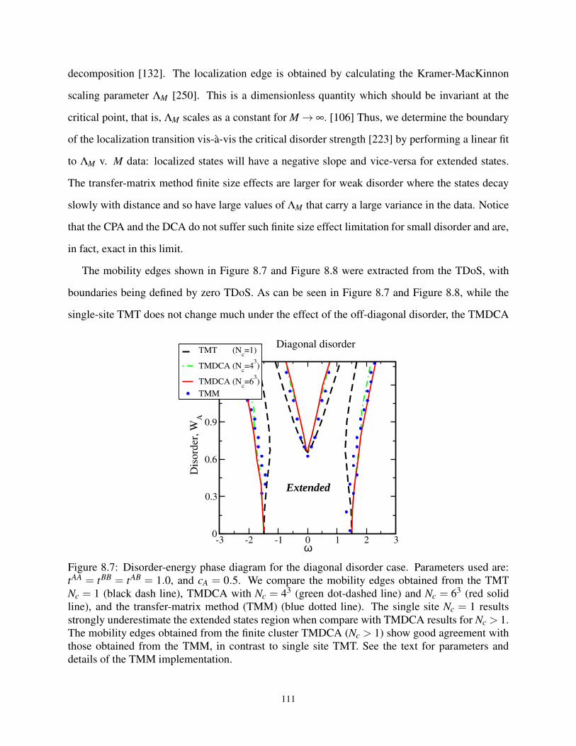
decomposition [132]. The localization edge is obtained by calculating the Kramer-MacKinnon
scaling parameter ΛM [250]. This is a dimensionless quantity which should be invariant at the
critical point, that is, ΛM scales as a constant for M → ∞. [106] Thus, we determine the boundary
of the localization transition vis-à-vis the critical disorder strength [223] by performing a linear fit
to ΛM v. M data: localized states will have a negative slope and vice-versa for extended states.
The transfer-matrix method finite size effects are larger for weak disorder where the states decay
slowly with distance and so have large values of ΛM that carry a large variance in the data. Notice
that the CPA and the DCA do not suffer such finite size effect limitation for small disorder and are,
in fact, exact in this limit.
The mobility edges shown in Figure 8.7 and Figure 8.8 were extracted from the TDoS, with
boundaries being defined by zero TDoS. As can be seen in Figure 8.7 and Figure 8.8, while the
single-site TMT does not change much under the effect of the off-diagonal disorder, the TMDCA
-3 -2 -1 0 1 2 3ω
0
0.3
0.6
0.9
1.2
D
isord
er, W
A
TMT (Nc=1)
TMDCA (Nc=4
3)
TMDCA (Nc=6
3)
TMM
Extended
Diagonal disorder
Figure 8.7: Disorder-energy phase diagram for the diagonal disorder case. Parameters used are:
tAA = tBB = tAB = 1.0, and cA = 0.5. We compare the mobility edges obtained from the TMT
Nc = 1 (black dash line), TMDCA with Nc = 43 (green dot-dashed line) and Nc = 63 (red solid
line), and the transfer-matrix method (TMM) (blue dotted line). The single site Nc = 1 results
strongly underestimate the extended states region when compare with TMDCA results for Nc > 1.
The mobility edges obtained from the finite cluster TMDCA (Nc > 1) show good agreement with
those obtained from the TMM, in contrast to single site TMT. See the text for parameters and
details of the TMM implementation.
111
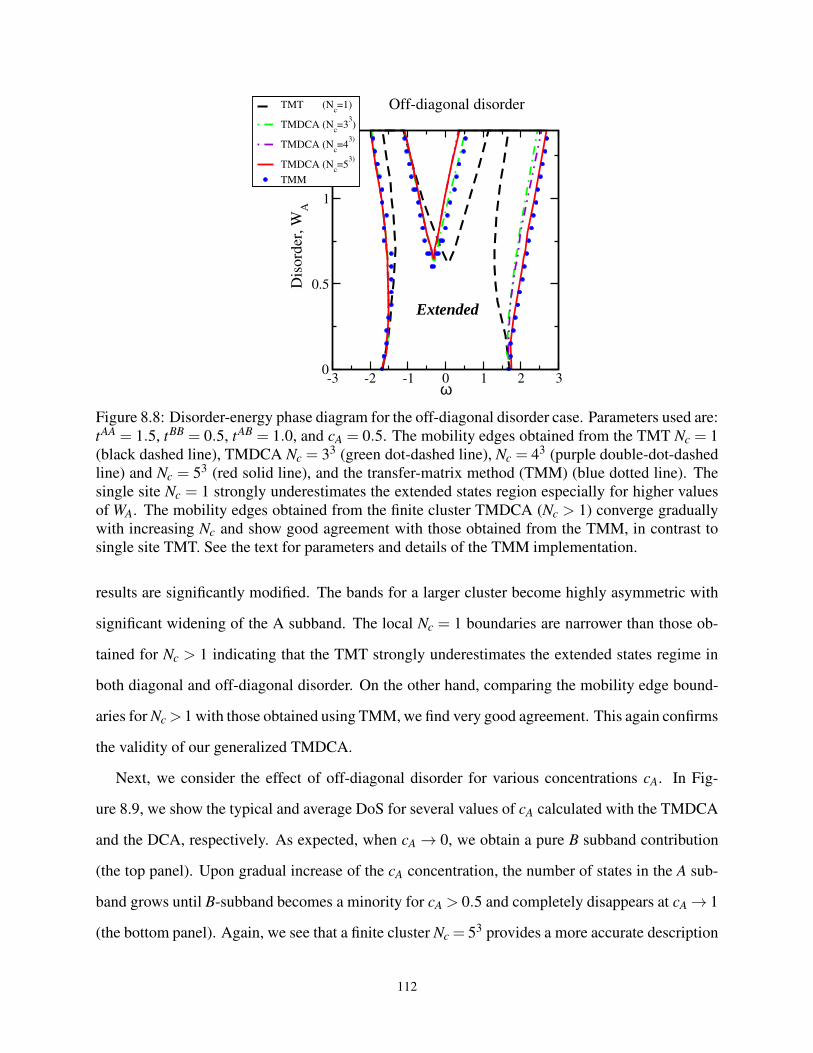
-3 -2 -1 0 1 2 3ω
0
0.5
1
D
isord
er, W
A
TMT (Nc=1)
TMDCA (Nc=3
3)
TMDCA (Nc=4
3)
TMDCA (Nc=5
3)
TMM
Extended
Off-diagonal disorder
Figure 8.8: Disorder-energy phase diagram for the off-diagonal disorder case. Parameters used are:
tAA = 1.5, tBB = 0.5, tAB = 1.0, and cA = 0.5. The mobility edges obtained from the TMT Nc = 1
(black dashed line), TMDCA Nc = 33 (green dot-dashed line), Nc = 43 (purple double-dot-dashed
line) and Nc = 53 (red solid line), and the transfer-matrix method (TMM) (blue dotted line). The
single site Nc = 1 strongly underestimates the extended states region especially for higher values
of WA. The mobility edges obtained from the finite cluster TMDCA (Nc > 1) converge gradually
with increasing Nc and show good agreement with those obtained from the TMM, in contrast to
single site TMT. See the text for parameters and details of the TMM implementation.
results are significantly modified. The bands for a larger cluster become highly asymmetric with
significant widening of the A subband. The local Nc = 1 boundaries are narrower than those ob-
tained for Nc > 1 indicating that the TMT strongly underestimates the extended states regime in
both diagonal and off-diagonal disorder. On the other hand, comparing the mobility edge bound-
aries for Nc > 1 with those obtained using TMM, we find very good agreement. This again confirms
the validity of our generalized TMDCA.
Next, we consider the effect of off-diagonal disorder for various concentrations cA. In Fig-
ure 8.9, we show the typical and average DoS for several values of cA calculated with the TMDCA
and the DCA, respectively. As expected, when cA → 0, we obtain a pure B subband contribution
(the top panel). Upon gradual increase of the cA concentration, the number of states in the A sub-
band grows until B-subband becomes a minority for cA > 0.5 and completely disappears at cA → 1
(the bottom panel). Again, we see that a finite cluster Nc = 53 provides a more accurate description
112
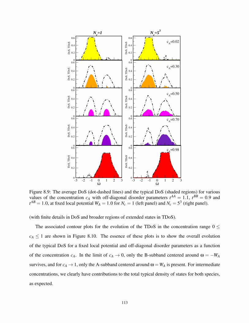
0
0.2
0.4
0.6
DoS
, T
DoS
0
0.2
0.4
0.6
DoS
, T
DoS
0
0.2
0.4
0.6
DoS
, T
DoS
0
0.2
0.4
0.6
DoS
, T
DoS
0
0.2
0.4
0.6
DoS
, T
DoS
-3 -2 -1 0 1 2 3ω
0
0.2
0.4
0.6
DoS
, T
DoS
0
0.2
0.4
0.6
DoS
, T
DoS
-3 -2 -1 0 1 2 3ω
0
0.2
0.4
0.6
DoS
, T
DoS
0
0.2
0.4
0.6
DoS
, T
DoS
0
0.2
0.4
0.6
DoS
, T
DoS
Nc=53
Nc=1
cA
=0.02
cA
=0.30
cA
=0.50
cA
=0.70
cA
=0.98
Figure 8.9: The average DoS (dot-dashed lines) and the typical DoS (shaded regions) for various
values of the concentration cA with off-diagonal disorder parameters tAA = 1.1, tBB = 0.9 and
tAB = 1.0, at fixed local potential WA = 1.0 for Nc = 1 (left panel) and Nc = 53 (right panel).
(with finite details in DoS and broader regions of extended states in TDoS).
The associated contour plots for the evolution of the TDoS in the concentration range 0 ≤
cA ≤ 1 are shown in Figure 8.10. The essence of these plots is to show the overall evolution
of the typical DoS for a fixed local potential and off-diagonal disorder parameters as a function
of the concentration cA. In the limit of cA → 0, only the B-subband centered around ω = −WA
survives, and for cA → 1, only the A-subband centered around ω =WA is present. For intermediate
concentrations, we clearly have contributions to the total typical density of states for both species,
as expected.
113
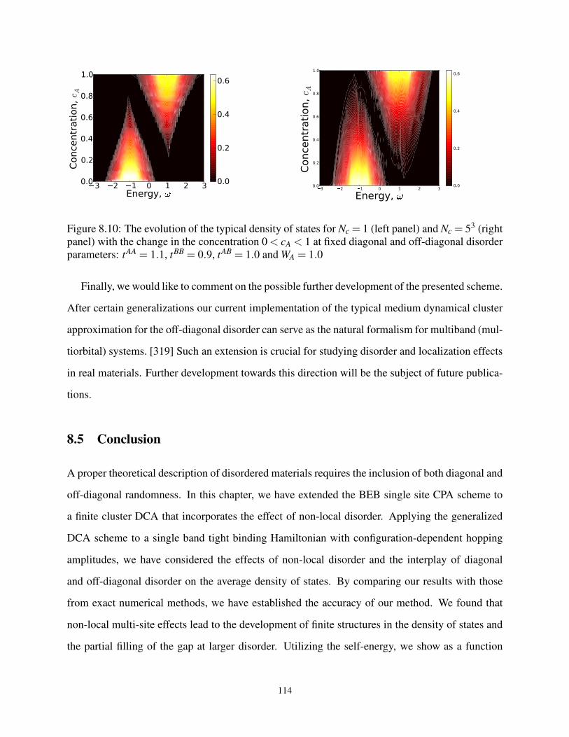
3 2 1 0 1 2 3Energy,
0.0
0.2
0.4
0.6
0.8
1.0Co
ncen
trat
ion,
c A
0.0
0.2
0.4
0.6
3 2 1 0 1 2 3
Energy, 0.0
0.2
0.4
0.6
0.8
1.0
Conc
entr
atio
n, c A
0.0
0.2
0.4
0.6
Figure 8.10: The evolution of the typical density of states for Nc = 1 (left panel) and Nc = 53 (right
panel) with the change in the concentration 0 < cA < 1 at fixed diagonal and off-diagonal disorder
parameters: tAA = 1.1, tBB = 0.9, tAB = 1.0 and WA = 1.0
Finally, we would like to comment on the possible further development of the presented scheme.
After certain generalizations our current implementation of the typical medium dynamical cluster
approximation for the off-diagonal disorder can serve as the natural formalism for multiband (mul-
tiorbital) systems. [319] Such an extension is crucial for studying disorder and localization effects
in real materials. Further development towards this direction will be the subject of future publica-
tions.
8.5 Conclusion
A proper theoretical description of disordered materials requires the inclusion of both diagonal and
off-diagonal randomness. In this chapter, we have extended the BEB single site CPA scheme to
a finite cluster DCA that incorporates the effect of non-local disorder. Applying the generalized
DCA scheme to a single band tight binding Hamiltonian with configuration-dependent hopping
amplitudes, we have considered the effects of non-local disorder and the interplay of diagonal
and off-diagonal disorder on the average density of states. By comparing our results with those
from exact numerical methods, we have established the accuracy of our method. We found that
non-local multi-site effects lead to the development of finite structures in the density of states and
the partial filling of the gap at larger disorder. Utilizing the self-energy, we show as a function
114
of increasing disorder strengths, the importance of a finite cluster in characterizing the Anderson
localization transition. For small disorder the single site and finite cluster results are essentially the
same, indicating that the CPA is a good approximation in the small disorder regime. However, for
a larger disorder we observe a significant momentum dependence in the self-energy resulting from
the non-local correlations which are incorporated in the DCA.
Electron localization for off-diagonal disorder models have not been studied from the typical
medium perspective. In this chapter, we generalized the TMDCA to systems with both diagonal
and off-diagonal disorder. Our developed method can quantitatively and qualitatively be used to
study the effects of disorder on the electron localization, effectively for systems with both diagonal
and off-diagonal randomness.
We show that within the TMDCA, the TDoS vanishes for localized states and is finite for
states which are extended. Employing the TDoS as an order parameter for Anderson localiza-
tion, we have constructed the disorder-energy phase diagram for systems with both diagonal and
off-diagonal disorder. We also demonstrate the inability of the single site CPA and the TMT meth-
ods to accurately capture the localization and disorder effects in both the average and the typical
DoS, respectively. We note that the single site TMT while being able to capture the behavior of
the diagonal and off-diagonal disorder, strongly underestimates the extended regions. Also the
TMT is less sensitive to the off-diagonal randomness with the mobility edges being only slightly
modified as compared to the diagonal case. In contrast, the finite cluster TMDCA results are able
to capture the considerable changes, with a pronounced asymmetry of the extended state region,
in the disorder-energy phase diagram under the effect of the off-diagonal disorder as compared to
the diagonal case. Most importantly, the TMDCA results are found to be in a quantitative agree-
ment with exact numerical results. Comparing our results with KPM, exact diagonalization, and
TMM, we find good agreement with our extended DCA and TMDCA. To the best of our knowl-
edge, this is the first numerically accurate investigation of the Anderson localization in systems
with off-diagonal disorder within the framework of the typical medium analysis. We believe that
the extended TMDCA scheme presents a powerful tool for treating both diagonal and off-diagonal
disorder on equal footing, and can be easily extended to study localization in multi-band systems.
115

Chapter 9
Application of Typical Medium Dynamical
Cluster Approximation to Multiband
Disordered System
9.1 Introduction
Diverse theoretical and numerical methods have been developed for studying disorder and corre-
lations in materials. For the single-band systems, many techniques/methods have been formulated
for tackling the many-body impurity. These computational techniques which are of varying com-
plexity not limited to exact numerical methods [320], quantum Monte Carlo (QMC) [321], numer-
ical renormalization group [322], and many other schemes [104, 255, 257, 261, 323]. However, for
realistic multiband systems, the impurity solver of choice have mainly being the QMC [324–326],
variants of the iterative perturbation theory [327–329], configuration interaction (CI) [323], and the
fluctuation exchange method (FLEX) [330]. However, due to the minus sign problem at low tem-
peratures [331], the QMC have been severely limited, and only applicable to Ising-like exchange
interactions. Note, there are other variants of the QMC formalism that do not suffer from the sign
problem (at least at the single-band level), for e.g., Ref. [332], and some other versions that work
with another exchange interactions, for e.g., a version of QMC with Hund’s exchange correla-
tions which work at two extreme limits: zero temperature [333] and at relatively high temperatures
(T & 1500K) [334]. The most realistic step in making the QMC applicable at low temperatures
have been the continuous-time QMC method [332, 335], and the Hirsch-Fye solver plus a pertur-
bation series expansion [336].
No doubt, these impurity/cluster solvers are powerful and are exact to within computational/statistical
errors, they do require the diagonalization of large lattices for any reasonable accuracy to be ob-
tained. Most importantly, most of these methods are developed in the Matsubara frequency as
such, requiring the analytical continuation of the data before real frequency information can be
116
accessed. There is no doubt that analytical continuation may introduce uncontrollable statistical
uncertainties, a typical ill-posed problem [337] but the Padé approximation [338] and maximum-
entropy method [337, 339] have been reported to produce reliable real frequency data. Aside the
Matsubara frequency based methods, one can work directly with other approximation methods that
work in the real frequency, such as the slave bosons, noncrossing approximation (NCA), numerical
renormalization group (NRG), exact diagonalization, and so on [104, 328, 340]. Each of the above
impurity solvers have their advantages and disadvantages. For example, exact diagonalization can
consider only a limited number of bath sites and cannot be adapted to study systems with inter-
actions, even an interaction as simple as a single impurity coupling, NRG is only reliable at low
energies, and NCA is limited to high temperatures.
For the study of localization transitions for multiband electronic systems, any of these impu-
rity/cluster solvers can be adapted. However, efforts so far have been limited to studying other
important material properties like antiferromagnetism, superconductivity, etc. But the ubiquity of
disorder is such that neglecting it is at one’s peril. Thus, a systematic incorporation of the effects
of disorder which is always present in varying forms in materials is paramount. Within the density
function theory community, variants of the supercell methods have been frequently used to study
the effects of disorder in materials [341, 342]. But still, they don’t characterize the localization
transitions.
In this Chapter, the typical medium theory will be recast for studying localization transitions
in a multiband systems, building on the successful formulated of the TMDCA for the single-band
system. Since the TMDCA formalism utilizes the DCA framework, it will first be formulated
within the DCA and then the TMDCA. Multiband becomes imperative as realistic materials have
orbital degrees of freedom. Unlike the single-band systems, multiband systems take into account
the influence of the localized electrons with orbital degrees of freedom.
117
9.2 Extension of the Single-band TMDCA to Multiband: Formalism
As a progress towards the application of the typical medium dynamical cluster approximation to
realistic systems, here, I will outline the steps needed to generalize the single-band TMDCA to
a two-band. Since the TMDCA uses the self-consistency of the dynamical cluster approximation
aside the utilization of an environment characterized by the typical medium, I will first generalize
the single band DCA to its multiband version and then to the TMDCA.
9.2.1 Multiband Formalism for Dynamical Cluster Approximation
For the multiband, the Hamiltonian (Equation 4.1) becomes
H = ∑<i, j>;αβ
t(αβ)i j (c†
iαc jβ + c†jαciβ)+∑
iα
(V(αβ)i −µ)n
(αβ)i − Jc ∑
i
Sisi. (9.1)
The first term provides a realistic multiband description of the host valence bands. The operators
c†i (ci) create (annihilate) a quasiparticle on site i. The second part denotes the disorder, which is
modeled by a local potential Vi that is randomly distributed according to some specified probability
distribution P(Vi), where ni = c†i ci is the number operator, µ is the chemical potential, i and j are
site indices, α,β label the bands (α,β = 1, ...,LB), LB is the number of bands, and t(αβ)i j is the
hopping matrix element
tαβi j = tα
i jδαβ +ϒδi j (9.2)
where tαδαβ is the orbital-dependent nearest-neighbor hopping and ϒ is the hybridization between
the two orbitals. We set 4t = 1 as the energy unit. Observe that for ϒ = 0, Equation 9.1 reduces
to multi-orbital Anderson model with distinct (decoupled) orbitals. The third part denotes the
interaction between itinerant carrier spins si and localized impurity spins Si (S = 5/2 for e.g.,
Mn2+). Jc is the local Hund’s coupling for e.g., Mn-d orbitals. For the time being, I will neglect
the coupling (Jc = 0).
For this study, an alloy model distributions (4.2d), which can be composed of many atoms
118
A1−xBCDEF...GxH or the familiar binary alloy model A1−xBx. Equation 4.2d then becomes
PMB(V(αβ)i ) = caδ(Vi −WA
αβ)+ cbδ(Vi −WBαβ). (9.3)
where cb = 1− ca is the concentration, WA and WB is the strength of the disorder, the subscript
MB denotes multiband, and the random potential becomes
Vi =
V ααi · · · V
αβi
. . .
. . .
. . .
Vβαi · · · V
ββi
(9.4)
For the single band, diagonal disorder model, the random potential is local in nature. However,
as it is obvious from Equation 9.4, the random potential here is both site and band dependent, and
also depends on the hopping amplitude of the electrons tαβi j
ti j =
tααi j , if i ∈ α, j ∈ α
tαβi j , if i ∈ α, j ∈ β
tβαi j , if i ∈ β, j ∈ α
tββi j , if i ∈ β, j ∈ β,
(9.5a)
which in momentum space (assuming only near-neighbor hopping) is nothing but a LB×LB matrix
(underbar denotes matrix) of the form
ε(K) =
Eαα0 + Nc
N ∑k εk · · · Eαβ0 + Nc
N ∑k εk
. . .
. . .
. . .
Eβα0 + Nc
N ∑k εk · · · Eββ0 + Nc
N ∑k εk
(9.5b)
119
where for a d-dimensional hypercubic lattice with a unit lattice spacing, εk = −2t ∑di coski, k =
(k1, ...,kd), and E0 is a local energy which can be used to shift the bands. Following the description
of the DCA framework, the first Brillouin zone is divided into Nc = Ld coarse-grained cells with
K centers surrounded by k-points within the cell such that k = K+ k. The DCA is characterized
by a non-local hybridization matrix function Γ(K,ω)
Γ(K,ω) =
Γαα(K,ω) · · · Γαβ(K,ω)
. . .
. . .
. . .
Γβα(K,ω) · · · Γββ(K,ω)
(9.6)
While the DCA is a K-dependent formalism, the cluster problem solve is always solved in real
space as to enable the incorporation of the disorder. For this, a stochastically generated random
configurations of the disorder potential V is used to calculate the cluster Green function which is
now an Nc ×Nc matrix as
Gi j =(
ωI− t ′(αβ)−Γ′(αβ)−V αβ)−1
i j(9.7)
where I is the identity matrix and the primes denote Fourier transform (FT) components of the
hybridization and hopping matrix, respectively. I.e.,
Γ′i j =
FT (Γαα(K,ω)), if i ∈ α, j ∈ α
FT (Γββ(K,ω)), if i ∈ β, j ∈ β
FT (Γαβ(K,ω)), if i ∈ α, j ∈ β
FT (Γβα(K,ω)), if i ∈ β, j ∈ α
(9.8a)
120

and
t ′i j =
FT (εαα(K)), if i ∈ α, j ∈ α
FT (εββ(K)), if i ∈ β, j ∈ β
FT (εαβ(K)), if i ∈ α, j ∈ β
FT (εβα(K)), if i ∈ β, j ∈ α
(9.8b)
where for e.g., FT (Γαβ(K,ω))=∑K Γαβ(K,ω)eiK(ri−r j). From Equation 9.8 Γ′αβi j and t ′
αβi j are now
Nc ×Nc real-space matrices. As explained in previous chapters, Γ′i j is a measure of the hybridiza-
tion (escape rate) between the sites/cluster i and j and the effective medium. Hence, intuitive, the
component of the bands αα of the hybridization rate corresponds to both bands α sitting at lattice
sites i and j. Similarly, the αβ bands imply that the site i and j is corresponds to the band α and
β, respectively. The description applies to t the ββ and βα. The hopping matrix shares the same
description above as the hybridization function.
To solve the cluster problem, we recast Equation 9.7 into an LBNc ×LBNc matrix and calculate
the disorder averaged cluster Green function
Gc(ω)i j =
〈Gααc (ω)〉i j · · ·
⟨
Gαβc (ω)
⟩
i j
. . .
. . .
. . .⟨
Gβαc (ω)
⟩
i j· · ·
⟨
Gββc (ω)
⟩
i j
(9.9)
which, can be done by assigning each components according to the band indices α and β of the
sites i and j
(Gααc )i j = (Gc)i j if i ∈ α, j ∈ α
(Gββc )i j = (Gc)i j if i ∈ β, j ∈ β
(Gαβc )i j = (Gc)i j if i ∈ α, j ∈ β
(Gβαc )i j = (Gc)i j if i ∈ β, j ∈ α (9.10)
121
Note, each of the diagonal bands in Equation 9.10 is normalized as a consequence of Equation 9.9
just like a conventional Green function. For example, a realistic cubic system with a perfect crystal
field splitting, Equation 9.9 corresponds to
Gc(ω)i j =
⟨
Gt2gc (ω)
⟩
i j0 0 0 0
0⟨
Gt2gc (ω)
⟩
i j0 0 0
0 0⟨
Gt2gc (ω)
⟩
i j0 0
0 0 0⟨G
egc (ω)
⟩
i j0
0 0 0 0⟨G
egc (ω)
⟩
i j
(9.11)
where t2g and eg correspond to the crystal field splitting of the d-orbital into the higher and lower
energy components, respectively. Having obtained the disorder averaged cluster Green functions
since the DCA is a K-space-based formalism, a Fourier transformation is to momentum space is
carried using Equation 9.10 as
Gc(K,ω) =
Gααc (K,ω) · · · G
αβc (K,ω)
. . .
. . .
. . .
Gβαc (K,ω) · · · G
ββc (K,ω)
(9.12)
Now that we have the K-dependent cluster Green functions, coarse-graining over the cluster cells
to obtain the lattice Green function
G(K,ω) =
Gαα(K,ω) · · · G
αβ(K,ω)
. . .
. . .
. . .
Gβα(K,ω) · · · G
ββ(K,ω)
=Nc
N∑k
(
Gc(K,ω)−1 +Γ(K,ω)− εk + ε(K))−1
,
(9.13)
122
where the overbar denotes cluster coarse-graining. Just as in Equation 9.10, the diagonal compo-
nents of Equation 9.13 have the same normalization of a conventional, i.e., scalar, Green function.
Since the DCA medium is characterized by the non-local hybridization functions, we close the
self-consistency loop by updating the corresponding hybridization functions for each band
Γαβn (K,ω) = Γαβ
o (K,ω)+ξ(
G−1c (K,ω)αβ−G
−1(K,ω)αβ
)
(9.14)
where ‘o’ and ‘n’ denote old and new, respectively, and ξ is a linear mixing parameter 0 < ξ < 1.
The above outlined steps are iterated until convergence using the DCA self-consistency require-
ments that the disorder averaged cluster and the coarse-grained lattice Green functions should be
equal
Gc(K,ω) = G(K,ω) . (9.15)
This is equivalent to a system of α×β coupled scalar equations
Gαβ(K,ω) = Gαβ
c (K,ω). (9.16)
For the case when tαβ = tβα, Gαβ(K,ω)=G
βα(K,ω) by default. At convergence, the hybridization
function also converges as Γαβn (K,ω) = Γ
αβo (K,ω).
9.2.2 Multiband Formalism for Typical Medium Dynamical Cluster Approximation
The dynamical cluster approximation incorporates all the important spatial correlations, improving
upon the capabilities of the local coherent potential approximation. However, for the characteriza-
tion of localization transitions, both the CPA, DCA, and other variants of the mean-field theory are
not adequate due mainly to the way their effective medium are defined. As demonstrated in Chap-
ters 7 and 6 (for the diagonal non-interacting system), Chapter 8 (for the diagonal and off-diagonal
non-interacting disordered system, and will be further confirmed in Chapter 10 (for the interacting
and disordered systems), the typical density of states (TDoS) if properly defined is the approxi-
mation order parameter for characterizing electron localization as it vanishes for states which are
localized and it is finite for extended states.
123
The task here will be the generalization of the scalar TMDCA into a matrix form. For the time
being, the focus will be only for two band model. Note, the original typical medium theory (TMT)
as well as the TMDCA are both ad hoc. The same can be said for its generalization to a multiband
system. However, in constructing the TMDCA ansatz both for the single-band and the multiband
systems, important physical limits must be satisfied. Those physical limits have been carefully
checked and indeed, the TMDCA (cf. Subsection 5.3.2) for both single-band and multiband are
systematic. For clarity, I will repeat them here: For Nc = 1, the TMDCA should reduce to the local
TMT scheme with ρctyp(ω) = exp〈lnρ(ω)〉; At weak disorder strength, W ≪ Wc, the real space
prefactor becomes 〈lnρi(ω,Vi)〉 ≈ ln〈ρi(ω,Vi)〉. Then ρctyp(K,ω) reduces to the DoS calculated
in DCA scheme, with ρctyp(K,ω) ≈ 〈ρc(K,ω,V)〉; above all, it should be causal and obey all the
qualities of a good cluster theory as outlined in Subsection 4.1.2.
Just as in the TMDCA analysis instead of using the algebraically averaged cluster Green func-
tion in the self-consistency loop, typical averaging is utilized. The scalar typical density of states
(cf. Equation 5.11) becomes a LB ×LB matrix
ρctyp(K,ω) =
exp
(1
Nc∑
Nc
i=1
⟨lnραα
ii (ω)⟩)
ϑαα · · · ϕαβ(ϑαβ)
. . .
. . .
. . .
ϕβα(ϑβα) · · · exp
(1
Nc∑
Nc
i=1
⟨
lnρββii (ω)
⟩)
ϑββ
(9.17)
124
where
ϑαα =
⟨ −1
πℑGαα
c (K,ω)
1Nc
∑Nc
i=1(−1
πℑGαα
ii (ω))
⟩
(9.18a)
ϑββ =
⟨ −1
πℑG
ββc (K,ω)
1Nc
∑Nc
i=1(−1
πℑG
ββii (ω))
⟩
(9.18b)
ϑαβ = ϑβα = exp
(
1
2Nc
Nc
∑i=1
(〈lnρααii (ω)〉+
⟨
lnρββii (ω)
⟩
)
)
(9.18c)
ϕαβ =
⟨ −1
πℑG
αβc (K,ω)
12Nc
∑Nc
i=1[(−1
πℑGαα
ii (ω))+(−1
πℑG
ββii (ω))]
⟩
(9.18d)
ϕβα =
⟨ −1
πℑG
βαc (K,ω)
12Nc
∑Nc
i=1[(−1
πℑGαα
ii (ω))+(−1
πℑG
ββii (ω))]
⟩
(9.18e)
To continue the self-consistency loop, a Hilbert transform of Equation 9.18 is carried out to obtain
the typical cluster Green function
Gc(K,ω) =
∫dω′ ραα
typ(K,ω′)ω−ω′ · · ·
∫dω′ ρ
βαtyp(K,ω′)ω−ω′
. . .
. . .
. . .
∫dω′ ρ
αβtyp(K,ω′)ω−ω′ · · ·
∫dω′ ρ
ββtyp(K,ω′)ω−ω′
(9.19)
and the disorder averaged cluster Green function is easily obtained from Equation 9.19. Once the
disorder averaged cluster Green function is obtained, the self-consistency loop continues just as
in the DCA for the multiband case as outlined in Subsection 9.2.1. The above sets of equations
provide the generalization of the TMDCA for the multiband systems.
Limiting Cases: As as explained above, the TMDCA for the multiband case must satisfy the
physical limiting cases as in the single band TMDCA, viz: i) Assuming no hybridization of any
form exists between the two bands, i.e., tαβ = 0 and W αβ = 0, this corresponds to two independent
125
bands each, being a single diagonal band since the off-diagonal bands in Equation 9.17 vanishes.
For Nc = 1, in this diagonal picture, the typical density of states reduces to the exponential prefactor
which is the exact form of the local TMT. ii) At weak disorder, the multiband TMDCA reduces to
the DCA multiband since the the geometrically averaged local prefactor of the TDoS numerically
cancels the algebraically averaged local term in the denominator of Equation 9.17. This is obvious
from the fact that exp(〈lnρi(ω,Vi)〉) ≈ exp(ln〈ρi(ω,Vi)〉) ⇒ 〈ρi(ω,Vi)〉. Unless stated otherwise,
in the subsequent sections, only two-bands will be considered so that α, β = 1,2.
9.3 Benchmarking the Multiband TMDCA with KPM
Just as in the case of the single band typical medium dynamical cluster approximation (TMDCA),
here, a comparison with numerically exact calculations using the kernel polynomial method (KPM)
will be carried out. This becomes imperative as to ascertain how the TMDCA benchmarks with
the KPM for various parameter regimes.
Figure 9.1 shows a comparison plot of the DCA (TMDCA) with the KPM for varying off-
diagonal disorder, Wab = 0.3 and 1.1, respectively at a fixed diagonal disorder strengths Wa =
Wb = 0.7 and zero inter-band hopping. Since the disorder strengths on bands 1 and 2 are the same,
only one band is shown for each parameter set. Observe that both the DCA and the TMDCA
compare rather well with the KPM data for both limits: weak inter-band disorder (Wab = 0.3)
and strong inter-band disorder (Wab = 1.1). Slight discrepancy is observed for the TMDCA data,
however, all critical points clearly benchmark well with the typical density of states from the
KPM. For the weak inter-band disorder coupling, Figure 9.1 resembles the single-band results (cf.
Chapter 8, Section 8.3). This is expected since the coupling between the bands is weak and they
tend to behave as two independent orbitals. However, as the disorder strength of the inter-band
is increased, additional two small peaks develop between the two large bands leading to a very
strong renormalization of the density of states. Observe further that the central gap opening at
the band center is maintained while a secondary gap appears at approximately at ω =±0.7 which
coincidentally, corresponds to the strength of the diagonal disorder strength on the bands.
126
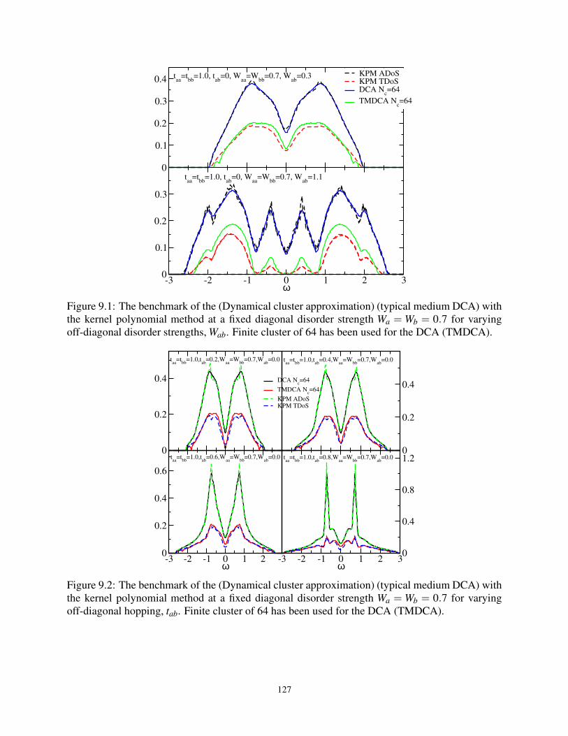
0
0.1
0.2
0.3
0.4
-3 -2 -1 0 1 2 3ω
0
0.1
0.2
0.3
KPM ADoSKPM TDoSDCA N
c=64
TMDCA Nc=64
taa
=tbb
=1.0, tab
=0, Waa
=Wbb
=0.7, Wab
=1.1
taa
=tbb
=1.0, tab
=0, Waa
=Wbb
=0.7, Wab
=0.3
Figure 9.1: The benchmark of the (Dynamical cluster approximation) (typical medium DCA) with
the kernel polynomial method at a fixed diagonal disorder strength Wa = Wb = 0.7 for varying
off-diagonal disorder strengths, Wab. Finite cluster of 64 has been used for the DCA (TMDCA).
0
0.2
0.4 DCA Nc=64
TMDCA Nc=64
KPM ADoSKPM TDoS
0
0.2
0.4
-3 -2 -1 0 1 2ω
0
0.2
0.4
0.6
-3 -2 -1 0 1 2 3ω
0
0.4
0.8
1.2
taa
=tbb
=1.0,tab
=0.2,Waa
=Wbb
=0.7,Wab
=0.0 taa
=tbb
=1.0,tab
=0.4,Waa
=Wbb
=0.7,Wab
=0.0
taa
=tbb
=1.0,tab
=0.6,Waa
=Wbb
=0.7,Wab
=0.0 taa
=tbb
=1.0,tab
=0.8,Waa
=Wbb
=0.7,Wab
=0.0
Figure 9.2: The benchmark of the (Dynamical cluster approximation) (typical medium DCA) with
the kernel polynomial method at a fixed diagonal disorder strength Wa = Wb = 0.7 for varying
off-diagonal hopping, tab. Finite cluster of 64 has been used for the DCA (TMDCA).
127
Some systems are inter-hopping dominated e.g., PdTe [343]. To check the applicability of the
developed multiband formalism for such systems, a comparison of the DCA (TMDCA) with their
KPM counterparts are depicted in Figure 9.2 for weak, intermediate, strong, and very strong inter-
band hopping, respectively, at a fixed on-site disorder strengths for bands 1 and 2, respectively.
Note, inter-band disorder strength is zero. Again, rather a good qualitative and quantitative bench-
mark with the KPM is observed. Both the ADoS and the TDoS from the DCA (TMDCA) and
the KPM both show a gap at ω = 0 for all parameter ranges while a secondary shoulder starts to
develop at the strong inter-band hopping value.
9.4 Conclusion
In this chapter, I have presented the extension of the dynamical cluster approximation (DCA) and
the typical medium DCA for applications in multi-band systems. In tandem with the objective of
this dissertation, which is to develop a method that is also applicable for realistic materials study,
the multi-band system becomes imperative as no system has a single-band. Various parameter
regimes are explored. It should be noted that these are the extreme of the parameter regimes. Most
importantly, the TMDCA results are found to be in a quantitative agreement with exact numerical
results. Comparing the results from kernel polynomial, remarkably good agreement with the DCA
and TMDCA are observed. The multi-band TMDCA offers a platform for doing realistic materials
simulations to study electron localization since the tight band parameters can be utilized directly.
128
Chapter 10
Application of Typical Medium Dynamical
Cluster Approximation to Interacting
Disordered Electron System
10.1 Introduction
In the absence of a spontaneous symmetry breaking field, the valence band of a half-filled non-
degenerate electron system may undergo a transition from a normal Fermi liquid (metal) to an
insulator (MIT) either due to randomness (disorder)(W ) [4, 35–37, 273] or Coulomb interactions
(U ) [38, 39].
A system with dominant electron correlation as compared to the kinetic energy undergoes a
transition from a metal to a correlation-induced insulator. This is known as the Mott MIT [38, 39]
where electrons are localized (trapped) on their individual atomic orbitals leading to the opening
of a gap in the single-particle spectra. Electron localization in strongly correlated systems can
also be induced by disorder (or randomness), which is inevitably present in real materials. This
phenomenon is known as Anderson MIT [4, 35–37]. Here, the transition from a metal to insula-
tor is not by the vanishing of the charge carriers but by the vanishing of the hybridization paths
accompanying the quantum localization of the wave functions due to the coherent backscattering
off random impurities. In contrast to the Mott MIT which is accompanied by the opening of a gap
in the single-particle spectra, the Anderson insulator is gapless indicating that the single-particle
excitations are essential in determining their physical properties especially at low energies.
The interplay of disorder [4, 35–37, 273] and interactions [38, 39] is an important problem in
diverse fields not limited to the physics of cold atoms, photonic and bosonic systems, and optical
lattices [40–43]. It has been actively studied both theoretically [17,44–50] and experimentally (see
for e.g., the metal-insulator transition of doped semiconductors [39, 51–53] and some perovskite
compounds [54–58]) for the past few decades.
129
Despite the vast theoretical and experimental studies, there are still many open questions. One
of such open questions is the metal-insulator-transitions (MIT) [37, 44, 69, 104] in the presence of
strong disorder and weak electron interactions and the parameter regime, which has remained one
of the most challenging problems of today’s condensed matter physics.
Many experimental studies [52,55–58] show that both disorder and interaction are essential for
the proper description of materials. Hence, any theoretical model formulated to understand MIT
must take into account both the effects of W and U on equal footing.
Naively, since both disorder and interactions, independently lead to a MIT, one would expect
their combined effects to be complimentary. In general, the opposite has been observed to be
the case especially at the extreme limits (strong W and small U , and vice-versa). Interacting
disordered electron systems show strong renormalization of the disorder strength [105] and hence
the reduction in the critical disorder strength [313] that may inhibit the development of the quasi-
coherent energy scale, already in the metallic state [102]. As such, there will be a non-trivial
renormalization of the critical disorder that may be different from those of the “pure” (U = 0)
Anderson MIT [12].
In this Chapter, I will focus on the effects of weak local interactions on disordered systems in
three dimensions. The approach is an extension of the developed typical medium-dynamical cluster
approximation (TMDCA) (cf. Chapter 7, which was shown to be highly successful in describing
the Anderson localization transition (ALT) for non-interacting systems [2]. The typical medium
approaches assume that the typical density of states (TDoS), when appropriately defined, acts as
the “proper” order parameter for the ALT. Such an assumption is well justified not only for the non-
interacting case [2,105,257] but also in the presence of interactions, as shown experimentally [52,
141]. The typical medium theory (TMT) of Dobrosavljevic et al. [105] is a special case of the
TMDCA when the cluster size Nc = 1. Even though the TMT cannot include weak localization
effects due to coherent backscattering, it still does qualitatively predict a disorder-driven ALT, and
hence incorporates ‘strong localization’ effects. The TMDCA incorporates non-local effects via
systematic finite cluster increment and achieves almost perfect agreement with numerical exact
calculations. The extension of the TMT to finite interactions show that interactions screen the
130
disorder [313, 344, 345]. I will show that such a conclusion is robust in the thermodynamic limit
through increasing cluster size calculations.
While there have been significant efforts to understand the combined effect of disorder and in-
teractions on the local density of states close to the Fermi level, the band edges have received scant
attention. Specifically, the effect of weak interactions on the mobility edge has not been discussed
thus far. This can be attributed to the difficulty in defining a proper mean-field order parameter ca-
pable of distinguishing between the delocalized and localized phases in the gapless single-particle
spectra of the Anderson-Mott insulator. The presence of electron interactions will further compli-
cate this already intricate situation due to the quantitatively different, low energy scales under this
coexistence with a nontrivial density of states (DoS) of the Anderson-Mott insulators. Moreover,
as the electron interaction “turns on”, singular diffusion modes lead to the mixing of states with
different energies.
The main result of this Chapter is that for µ < ωε, arbitrary small interactions lead to the mask-
ing of the sharp mobility edge that separates localized and extended states in the non-interacting
regime below the critical disorder strength WU=0c . Thus, interactions can radically modify the spec-
trum of a non-interacting system even at the band edges, i.e., in the ‘localized band’. However,
when the chemical potential (µ) is outside the mobility edge energy (i.e., µ > ωε), the well-defined
localization edge is restored. Nevertheless, unlike the non-interacting systems where the TDoS just
shifts rigidly as one scans through µ, in the presence of interactions, there is a non-trivial decrease
of the TDoS vis-à-vis the change in the filling. Further, we predict a soft-pseudogap at intermedi-
ate W just below WUc in agreement with experiments [54, 55]. The typical medium for interacting
disordered electron system is a self-consistent, systematic formalism for treating both disorder and
interactions at equal and to allow for their mutual renormalization effects.
10.2 Formalism and Method
The Anderson-Hubbard model is a minimal model for studying the interplay between electron–
electron interactions and disorder. The Hamiltonian for this model is defined by Equation 4.4.
131
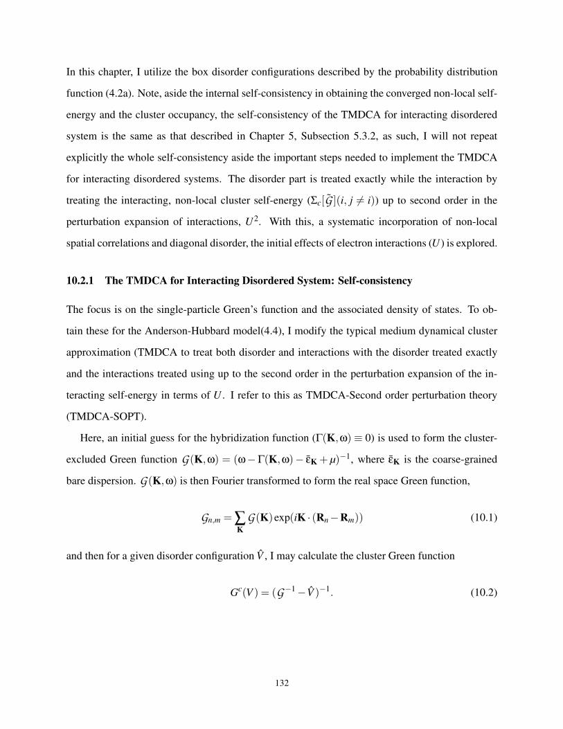
In this chapter, I utilize the box disorder configurations described by the probability distribution
function (4.2a). Note, aside the internal self-consistency in obtaining the converged non-local self-
energy and the cluster occupancy, the self-consistency of the TMDCA for interacting disordered
system is the same as that described in Chapter 5, Subsection 5.3.2, as such, I will not repeat
explicitly the whole self-consistency aside the important steps needed to implement the TMDCA
for interacting disordered systems. The disorder part is treated exactly while the interaction by
treating the interacting, non-local cluster self-energy (Σc[G ](i, j 6= i)) up to second order in the
perturbation expansion of interactions, U2. With this, a systematic incorporation of non-local
spatial correlations and diagonal disorder, the initial effects of electron interactions (U ) is explored.
10.2.1 The TMDCA for Interacting Disordered System: Self-consistency
The focus is on the single-particle Green’s function and the associated density of states. To ob-
tain these for the Anderson-Hubbard model(4.4), I modify the typical medium dynamical cluster
approximation (TMDCA to treat both disorder and interactions with the disorder treated exactly
and the interactions treated using up to the second order in the perturbation expansion of the in-
teracting self-energy in terms of U . I refer to this as TMDCA-Second order perturbation theory
(TMDCA-SOPT).
Here, an initial guess for the hybridization function (Γ(K,ω) ≡ 0) is used to form the cluster-
excluded Green function G(K,ω) = (ω−Γ(K,ω)− εK + µ)−1, where εK is the coarse-grained
bare dispersion. G(K,ω) is then Fourier transformed to form the real space Green function,
Gn,m = ∑K
G(K)exp(iK · (Rn−Rm)) (10.1)
and then for a given disorder configuration V , I may calculate the cluster Green function
Gc(V ) = (G−1 −V )−1. (10.2)
132
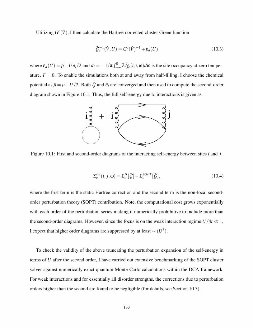
Utilizing Gc(V ), I then calculate the Hartree-corrected cluster Green function
G−1c (V ,U) = Gc(V )−1 + εd(U) (10.3)
where εd(U) = µ−Uni/2 and ni = −1/π∫ 0−∞ ℑGc(i, i,ω)dω is the site occupancy at zero temper-
ature, T = 0. To enable the simulations both at and away from half-filling, I choose the chemical
potential as µ = µ+U/2. Both G and ni are converged and then used to compute the second-order
diagram shown in Figure 10.1. Thus, the full self-energy due to interactions is given as
i ji +
Figure 10.1: First and second-order diagrams of the interacting self-energy between sites i and j.
ΣIntc (i, j,ω) = ΣH
c [G ]+ΣSOPTc [G ], (10.4)
where the first term is the static Hartree correction and the second term is the non-local second-
order perturbation theory (SOPT) contribution. Note, the computational cost grows exponentially
with each order of the perturbation series making it numerically prohibitive to include more than
the second-order diagrams. However, since the focus is on the weak interaction regime U/4t ≪ 1,
I expect that higher order diagrams are suppressed by at least ∼ (U3).
To check the validity of the above truncating the perturbation expansion of the self-energy in
terms of U after the second order, I have carried out extensive benchmarking of the SOPT cluster
solver against numerically exact quantum Monte-Carlo calculations within the DCA framework.
For weak interactions and for essentially all disorder strengths, the corrections due to perturbation
orders higher than the second are found to be negligible (for details, see Section 10.3).
133
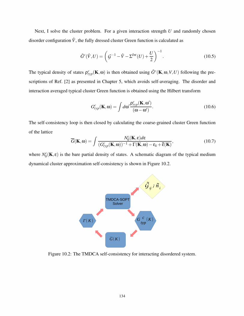
Next, I solve the cluster problem. For a given interaction strength U and randomly chosen
disorder configuration V , the fully dressed cluster Green function is calculated as
Gc(V ,U) =
(
G−1 −V −ΣInt(U)+U
2
)−1
. (10.5)
The typical density of states ρctyp(K,ω) is then obtained using Gc(K,ω,V,U) following the pre-
scriptions of Ref. [2] as presented in Chapter 5, which avoids self-averaging. The disorder and
interaction averaged typical cluster Green function is obtained using the Hilbert transform
Gctyp(K,ω) =
∫dω′ρ
ctyp(K,ω′)
(ω−ω′). (10.6)
The self-consistency loop is then closed by calculating the coarse-grained cluster Green function
of the lattice
G(K,ω) =∫
Nc0(K,ε)dε
(Gctyp(K,ω))−1+Γ(K,ω)− εk + ε(K)
, (10.7)
where Nc0(K,ε) is the bare partial density of states. A schematic diagram of the typical medium
dynamical cluster approximation self-consistency is shown in Figure 10.2.
Figure 10.2: The TMDCA self-consistency for interacting disordered system.
134
10.2.2 Advantages of the TMDCA for Interacting Disorder System
Aside the very small computational cost and the possibility of incorporating materials specific
details even for interacting disorder systems provided by the typical medium dynamical cluster ap-
proximations, there are obvious many other advantages when compared specifically to Matsubara
frequency based methods. Notice that in the formulation of the typical medium dynamical cluster
approximation and the average medium based dynamical cluster approximation for studying the
Anderson–Hubbard Hamiltonian(4.4), instead of using the conventional Matsubara frequency ap-
proach, I instead, reformulated the formalism in real frequency. This has the major advantage of
not only being capable of capturing finite temperature (T ) physics, but well suited for T = 0, where
Matsubara-based approaches cannot be used. It also avoids the rigor of analytical continuation of
the major observables: the Green function and the self-energy. To achieve these, recall that the
second order perturbation theory self-energy is the expansion up to the second order in U (O[U2])
around the Hartree-corrected host propagator given as
Σintc (i, j,ω) = ΣH
c [G ]+Σ(SOPT)c [G ] (10.8)
where i and j are site indices. The first term of the Hamiltonian ΣHc [G ] =Uni/2 is the Hartree term
while the second term is the density-density term which in the Matsubara frequency is given by
Σ(SOPT)c [G ] =− lim
iω→ω+
[
U2
N2c β2 ∑
m,p,P,Q
G(K+Q, iωn+ iνm)G(P+Q, iωp+ iνm)G(P, iωp)
]
.
(10.9)
However, since the cluster problem is solved in real space and for the fact that it is numerically
more advantageous to work in the real frequency than in the Matsubara frequency (because analytic
continuation has to be carried out from the imaginary frequency to the real frequency in order to
get real frequency quantities), one can transform Equation 10.9 to its real frequency representation
135
as outlined in Appendix E. Equation 10.9 in real frequency (suppressing site indices) is then
ρΣ(ω) = U2∫
dε1dε2ρG (ε1)ρG(ω− ε1 + ε2)ρG(ε2)
×[n f (−ε1)n f (ε2)n f (−ω+ ε1 − ε2)+n f (ε1)n f (−ε2)n f (ω− ε1 + ε2)
](10.10)
where ρG = −1/πℑG , n f = 1/(eβε +1) is the Fermi function, and Q, P, K are cluster momenta.
We note that ρG vanishes only for |ω| ≥ 3B/2 [346], where B is the full bandwidth (12t = 3 in
our unit). The real part of the second-order term of the ISE ΣSOPTR (i, j,ω) on each cluster site is
obtained via the Hilbert transform, and the non-local SOPT self-energy is then obtained as
ΣSOPTc (i, j,ω) = ΣSOPT
R (i, j,ω)− iπρΣ(i, j,ω) (10.11)
Note that Equation 10.10 scales as an O[N3], where N is the number of the grid points used for the
integration. In my computations, this N3 process is dramatically reduced to scale logarithmically
as N lnN using fast Fourier transformation [347].
10.3 Benchmarking TMDCA-SOPT with CTQMC in Three Dimensions
To validate the TMDCA developed for characterizing interacting disordered system and check its
suitability for studying the interacting disordered electron system, I compare the results for the
Anderson-Hubbard model at half-filling with results from the dynamical cluster approximation
(DCA) using the continuous-time quantum Monte Carlo method (CTQMC) [335, 348–351].
The quantum Monte Carlo (QMC) methods are powerful tools that enable controlled calcula-
tions of the properties of large quantum many-particle systems. Details of the CTQMC formalisms
are well described in the literature (see for e.g., Refs. [321,335,348–352]) as such, and we will not
attempt to give a detailed description of the algorithms here but will just give an overview which en-
ables us to compare the QMC results with our Hilbert transformed imaginary frequency data. In the
CTQMC, to avoid any possible time discretization error in the imaginary time axis, we adopt the
recent improvements in the QMC algorithms in the continuous imaginary time [335,348,350,352].
136

This significantly improves the quality of the data.
To make the comparison, I convert the real frequency data to Matsubara frequency using the
Hilbert transformation, and obtain the local Green function and self-energy, respectively, as
Gloc(iωn) =−1
π
∫ ∞
−∞dω
ℑGloc(ω)
iωn −ω; Σloc(iωn) =−1
π
∫ ∞
−∞dω
ℑΣloc(ω)
iωn −ω(10.12)
where ωn = (2n+1)π/β with β = 1/kBT and n ∈Z is the fermionic Matsubara frequency, T is the
temperature (in a unit of 4t), and kB = 1 is the universal Boltzmann’s constant.
10.3.1 Limit of Zero Disorder: Hubbard Model
0 1 2 3ω
n
-1.6
-1.2
-0.8
-0.4
U=0.5U=0.75U=1.5
0.16 0.4 1ω
n
10-3
10-2
10-1
U=0.1U=0.2U=0.4U=0.5U=0.75U=1.5
-1.6
-1.2
-0.8
-0.4
0
U=0.4U=0.5U=0.75U=1.5
A
AA A A A A A A10
-3
10-2
10-1
U=0.4U=0.5U=0.75U=1.5U=0.1A A
U=0.2
ℑG
loc(i
ωn)
-ℑΣlo
c(iω
n)
(a)
(b) (d)
(c)
Nc=1 N
c=1
Nc=14N
c=14
Figure 10.3: The comparison of the single-particle quantities from TMDCA-SOPT and DCA-
CTQMC at T = 0.025 for the half-filled Hubbard model (zero disorder and the finite Coulomb
interaction U > 0). The comparison of the imaginary part of the local self-energy for Nc = 1 (a)
and Nc = 14 (b), respectively, on a log-log scale. Also shown is the corresponding comparison of
the local Green function for Nc = 1 (c) and Nc = 14 (d), respectively on a linear scale. Smaller
values (U < 0.3 for Nc = 1) and (U < 0.4 for Nc = 14) are not shown on the local Green functions
plot for easy readability as they are too close to each other. In both cases, the dotted lines with
symbols are for the TMDCA-SOPT while the solid lines depict the DCA-CTQMC results. Further,
for the self-energy plots, smaller interaction strengths (U ≤ 0.5) are on top of each other and as
such, may appear indistinguishable.
At zero disorder strength, W = 0, the Anderson-Hubbard model (Equation 4.4) reduces to the
137
Hubbard Hamiltonian (Equation 4.3). As a natural consequence, the self-energy of the Hubbard
model of the numerically exact CTQMC contains the most vital information for benchmarking
with a mean-field theory like the TMDCA-SOPT. I show in Figs. 10.3(a) and 10.3(b) the com-
parison plots of the TMDCA-SOPT (using Equation 10.12) as compared with the CTQMC data
for the Nc = 1 and finite cluster of 14, respectively, at various values of the interaction. As it is
evident from the plots, the data benchmarks well up to U ∼ 2.25 for Nc = 1 and U ∼ 0.75 for
Nc = 14 showing both quantitative and qualitative agreement between the TMDCA-SOPT and the
CTQMC results. The remarkable exact agreement between the TMDCA-SOPT and CTQMC for
low U (≤ 0.75), at all frequencies for both single-site and finite cluster shows that the self-energy
from the TMDCA-SOPT has the correct behavior and as such, ensures that the conclusions arrived
earlier about the expansion of the self-energy up to second order to be enough to quantify the
weakly interacting disordered system to be numerically correct. At least for the smaller U -values
(which is the regime of interest here), the good agreement with CTQMC further shows that the per-
turbation expansion of the self-energy up to O[U2]
in U should capture all the dominant quantum
fluctuations guaranteeing that quantitatively correct results are obtained. Hence, the results I will
present in the subsequent sections for small interacting disordered electron system are accurate to
within the computational accuracy of the formalism.
I further show in Figs. 10.3(c) and 10.3(d), the plot of the imaginary local Green function
from the TMDCA-SOPT (transformed from real to Matsubara frequency using Equation 10.12)
as compared to the CTQMC data for T = 0.025 and W = 0 for the Nc = 1 and Nc = 14, respec-
tively. Again, as a confirmation of the good agreement in the local self-energy, the local Green
function from the two methods are numerically the same especially for the small U -values. They
are practically on top of each other up to U ≈ 1.50 for both Nc = 1 and 14.
10.3.2 Limit of finite Disorder and Interaction: Anderson-Hubbard Model
To further check the applicability of the expansion of the interacting self-energy in powers of
Coulomb interactions, U , up to the second-order for the study of disordered interacting elec-
tron system, I further benchmark the developed method for the Anderson-Hubbard model (Equa-
138
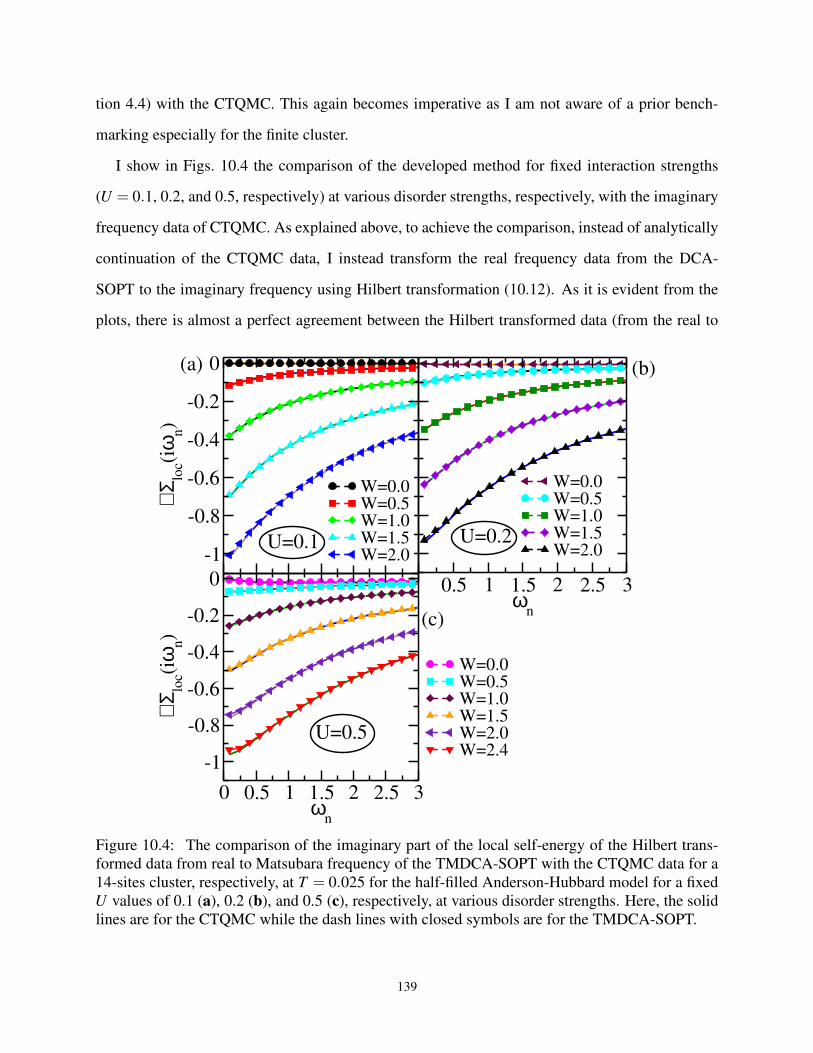
tion 4.4) with the CTQMC. This again becomes imperative as I am not aware of a prior bench-
marking especially for the finite cluster.
I show in Figs. 10.4 the comparison of the developed method for fixed interaction strengths
(U = 0.1, 0.2, and 0.5, respectively) at various disorder strengths, respectively, with the imaginary
frequency data of CTQMC. As explained above, to achieve the comparison, instead of analytically
continuation of the CTQMC data, I instead transform the real frequency data from the DCA-
SOPT to the imaginary frequency using Hilbert transformation (10.12). As it is evident from the
plots, there is almost a perfect agreement between the Hilbert transformed data (from the real to
0 0.5 1 1.5 2 2.5 3ω
n
-1
-0.8
-0.6
-0.4
-0.2
0
ℑΣlo
c(iω
n)
W=0.0W=0.5W=1.0W=1.5W=2.0W=2.4
0.5 1 1.5 2 2.5 3ω
n
W=0.0W=0.5W=1.0W=1.5W=2.0-1
-0.8
-0.6
-0.4
-0.2
0
ℑΣlo
c(iω
n)
W=0.0W=0.5W=1.0W=1.5W=2.0
U=0.2U=0.1
(a)
U=0.5
(b)
(c)
Figure 10.4: The comparison of the imaginary part of the local self-energy of the Hilbert trans-
formed data from real to Matsubara frequency of the TMDCA-SOPT with the CTQMC data for a
14-sites cluster, respectively, at T = 0.025 for the half-filled Anderson-Hubbard model for a fixed
U values of 0.1 (a), 0.2 (b), and 0.5 (c), respectively, at various disorder strengths. Here, the solid
lines are for the CTQMC while the dash lines with closed symbols are for the TMDCA-SOPT.
139
Matsubara frequency) with the CTQMC results even for a relatively large value of the interaction
strengths (U ∼ 0.5) for all the disorder strengths up to the localization transitions. This further
confirms that our truncation of the perturbation series expansion of the interacting self-energy at
O[U2]
(at least in the weak interaction regime) is enough to account for the quantum fluctuations
in the typical environment. One can thus affirm that at least, within the weak interaction regime
(U/4t ≪ 1) in a disordered electron system that higher order diagrams in the expansion of the Σintc
are suppressed by at least ∼ (U3).
10.4 Weakly Interacting Disordered System in Three-Dimensions
In three-dimensional systems for the non-interacting case, there is a broad, well-defined metal-
insulator-transitions (MIT) of the gapless Anderson spectra at a given critical disorder strength
WU=0c . Here, we systematically analyze what happens to this spectra as interaction is gradually
turned on. Below, we present some results for the weakly interacting disordered three-dimensional
systems.
10.4.1 The DoS for Weakly Interacting Disordered System in Three Dimension
To kick start the discussion of the results obtained by applying the typical medium dynamical
cluster approximation to the study of weakly interacting disordered systems, I show in Figs. 10.5(a)
and (b) for a finite cluster Nc = 38 at various disorder strengths for U = 0.0 and 0.1 at half-filling,
the comparison of the algebraic (or average) density of states (ADoS) (obtained from the DCA,
where the algebraic averaging is utilized in the self-consistency) and the typical density of states
(TDoS) (obtained from the TMDCA-SOPT, where the self-consistency environment is defined by
a typical medium).
At weak disorder, W ∼ 0.5, the TDoS resembles the ADoS. However, for larger W , comparing
the U = 0.0 results (Figure 10.5(a)) with those of U = 0.1 (Figure 10.5(b)), a noticeable renormal-
ization of the spectrum is observed. There is a gradual suppression of the TDoS as the disorder
strength is increased for both U = 0.0 and 0.1. The TDoS at ω = 0 is noticeably higher when the
140
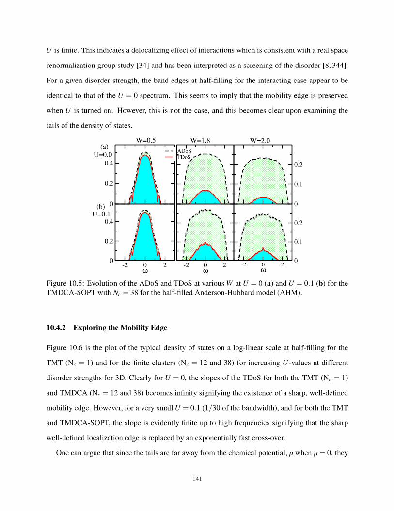
U is finite. This indicates a delocalizing effect of interactions which is consistent with a real space
renormalization group study [34] and has been interpreted as a screening of the disorder [8, 344].
For a given disorder strength, the band edges at half-filling for the interacting case appear to be
identical to that of the U = 0 spectrum. This seems to imply that the mobility edge is preserved
when U is turned on. However, this is not the case, and this becomes clear upon examining the
tails of the density of states.
0
0.2
0.4
-2 0 2ω
0
0.2
0.4
ADoSTDoS
0
0.1
0.2
-2 0 2ω
0
0.1
0.2
-2 0 2ω
U=0.0
U=0.1
W=0.5(a)
(b)
W=1.8 W=2.0
Figure 10.5: Evolution of the ADoS and TDoS at various W at U = 0 (a) and U = 0.1 (b) for the
TMDCA-SOPT with Nc = 38 for the half-filled Anderson-Hubbard model (AHM).
10.4.2 Exploring the Mobility Edge
Figure 10.6 is the plot of the typical density of states on a log-linear scale at half-filling for the
TMT (Nc = 1) and for the finite clusters (Nc = 12 and 38) for increasing U -values at different
disorder strengths for 3D. Clearly for U = 0, the slopes of the TDoS for both the TMT (Nc = 1)
and TMDCA (Nc = 12 and 38) becomes infinity signifying the existence of a sharp, well-defined
mobility edge. However, for a very small U = 0.1 (1/30 of the bandwidth), and for both the TMT
and TMDCA-SOPT, the slope is evidently finite up to high frequencies signifying that the sharp
well-defined localization edge is replaced by an exponentially fast cross-over.
One can argue that since the tails are far away from the chemical potential, µ when µ = 0, they
141
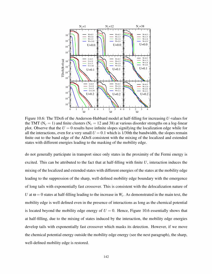
10-5
10-4
10-3
10-1 W=0.5
W=1.0
W=1.5
W=1.62
W=0.5
W=1.5
W=1.8
W=2.0
W=0.5
W=1.5
W=1.8
W=2.0
0 1 2 3 4ω
10-5
10-4
10-3
10-1
U=0.5
U=1.0
U=1.5
U=1.85
10-5
10-4
10-3
10-1
TD
oS
(R=
0;ω
) U=0.5
U=1.0
U=1.5
U=1.62
0 1 2 3 4ω
W=0.5
W=1.8
W=2.0
W=2.2
W=0.5
W=1.5
W=1.8
W=2.0
W=0.5
W=1.5
W=1.8
W=2.0
0 1 2 3 4ω
W=0.5
W=1.8
W=2.0
W=2.2
Nc=1 N
c=12 N
c=38
U=0.0
U=0.1
U=0.2
U=0.0 U=0.0
U=0.1 U=0.1
U=0.2 U=0.2
Figure 10.6: The TDoS of the Anderson-Hubbard model at half-filling for increasing U -values for
the TMT (Nc = 1) and finite clusters (Nc = 12 and 38) at various disorder strengths on a log-linear
plot. Observe that the U = 0 results have infinite slopes signifying the localization edge while for
all the interactions, even for a very small U = 0.1 which is 1/30th the bandwidth, the slopes remain
finite out to the band edge of the ADoS consistent with the mixing of the localized and extended
states with different energies leading to the masking of the mobility edge.
do not generally participate in transport since only states in the proximity of the Fermi energy is
excited. This can be attributed to the fact that at half-filling with finite U , interaction induces the
mixing of the localized and extended states with different energies of the states at the mobility edge
leading to the suppression of the sharp, well-defined mobility edge boundary with the emergence
of long tails with exponentially fast crossover. This is consistent with the delocalization nature of
U at ω = 0 states at half-filling leading to the increase in Wc. As demonstrated in the main text, the
mobility edge is well defined even in the presence of interactions as long as the chemical potential
is located beyond the mobility edge energy of U = 0. Hence, Figure 10.6 essentially shows that
at half-filling, due to the mixing of states induced by the interaction, the mobility edge energies
develop tails with exponentially fast crossover which masks its detection. However, if we move
the chemical potential energy outside the mobility edge energy (see the next paragraph), the sharp,
well-defined mobility edge is restored.
142
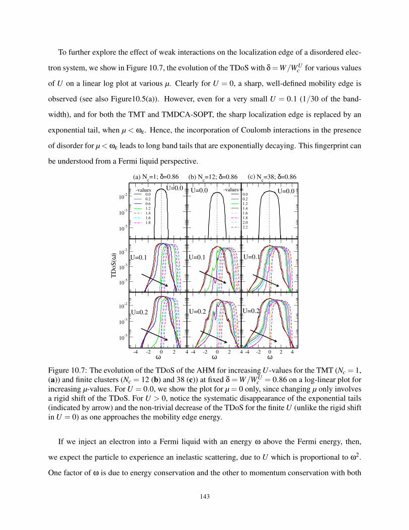
To further explore the effect of weak interactions on the localization edge of a disordered elec-
tron system, we show in Figure 10.7, the evolution of the TDoS with δ =W/WUc for various values
of U on a linear log plot at various µ. Clearly for U = 0, a sharp, well-defined mobility edge is
observed (see also Figure10.5(a)). However, even for a very small U = 0.1 (1/30 of the band-
width), and for both the TMT and TMDCA-SOPT, the sharp localization edge is replaced by an
exponential tail, when µ < ωε. Hence, the incorporation of Coulomb interactions in the presence
of disorder for µ < ωε leads to long band tails that are exponentially decaying. This fingerprint can
be understood from a Fermi liquid perspective.
10-5
10-3
10-2
-4 -2 0 2 4ω
10-5
10-3
10-2
10-5
10-3
10-2
TD
oS
(ω)
0.0
0.2
0.6
1.2
1.4
1.6
1.8
-4 -2 0 2 4ω
0.0
0.2
1.2
1.4
1.6
1.8
2.0
2.2
-4 -2 0 2 4ω
Nc=1; δ=0.86 N
c=12; δ=0.86 N
c=38; δ=0.86
U=0.0
U=0.1
U=0.2
U=0.0 U=0.0
U=0.1 U=0.1
U=0.2 U=0.2
m -values m -values
(a) (b) (c)
Figure 10.7: The evolution of the TDoS of the AHM for increasing U -values for the TMT (Nc = 1,
(a)) and finite clusters (Nc = 12 (b) and 38 (c)) at fixed δ =W/WUc = 0.86 on a log-linear plot for
increasing µ-values. For U = 0.0, we show the plot for µ = 0 only, since changing µ only involves
a rigid shift of the TDoS. For U > 0, notice the systematic disappearance of the exponential tails
(indicated by arrow) and the non-trivial decrease of the TDoS for the finite U (unlike the rigid shift
in U = 0) as one approaches the mobility edge energy.
If we inject an electron into a Fermi liquid with an energy ω above the Fermi energy, then,
we expect the particle to experience an inelastic scattering, due to U which is proportional to ω2.
One factor of ω is due to energy conservation and the other to momentum conservation with both
143
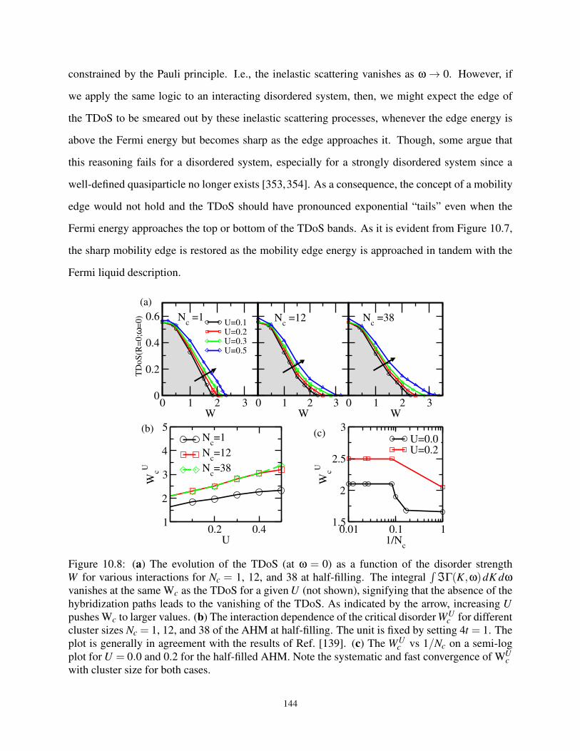
constrained by the Pauli principle. I.e., the inelastic scattering vanishes as ω → 0. However, if
we apply the same logic to an interacting disordered system, then, we might expect the edge of
the TDoS to be smeared out by these inelastic scattering processes, whenever the edge energy is
above the Fermi energy but becomes sharp as the edge approaches it. Though, some argue that
this reasoning fails for a disordered system, especially for a strongly disordered system since a
well-defined quasiparticle no longer exists [353,354]. As a consequence, the concept of a mobility
edge would not hold and the TDoS should have pronounced exponential “tails” even when the
Fermi energy approaches the top or bottom of the TDoS bands. As it is evident from Figure 10.7,
the sharp mobility edge is restored as the mobility edge energy is approached in tandem with the
Fermi liquid description.
0 1 2 3W
0 1 2 3W
0
0.2
0.4
0.6U=0.1U=0.2U=0.3U=0.5
0 1 2 3W
0.01 0.1 11/N
c
1.5
2
2.5
3
WcU
U=0.0U=0.2
0.2 0.4U
1
2
3
4
5
WcU
Nc=1
Nc=12
Nc=38
Nc =1 N
c =12 N
c =38
TD
oS
(R=
0;ω
=0)
(a)
(b) (c)
Figure 10.8: (a) The evolution of the TDoS (at ω = 0) as a function of the disorder strength
W for various interactions for Nc = 1, 12, and 38 at half-filling. The integral∫
ℑΓ(K,ω)dK dωvanishes at the same Wc as the TDoS for a given U (not shown), signifying that the absence of the
hybridization paths leads to the vanishing of the TDoS. As indicated by the arrow, increasing U
pushes Wc to larger values. (b) The interaction dependence of the critical disorder WUc for different
cluster sizes Nc = 1, 12, and 38 of the AHM at half-filling. The unit is fixed by setting 4t = 1. The
plot is generally in agreement with the results of Ref. [139]. (c) The WUc vs 1/Nc on a semi-log
plot for U = 0.0 and 0.2 for the half-filled AHM. Note the systematic and fast convergence of WUc
with cluster size for both cases.
144
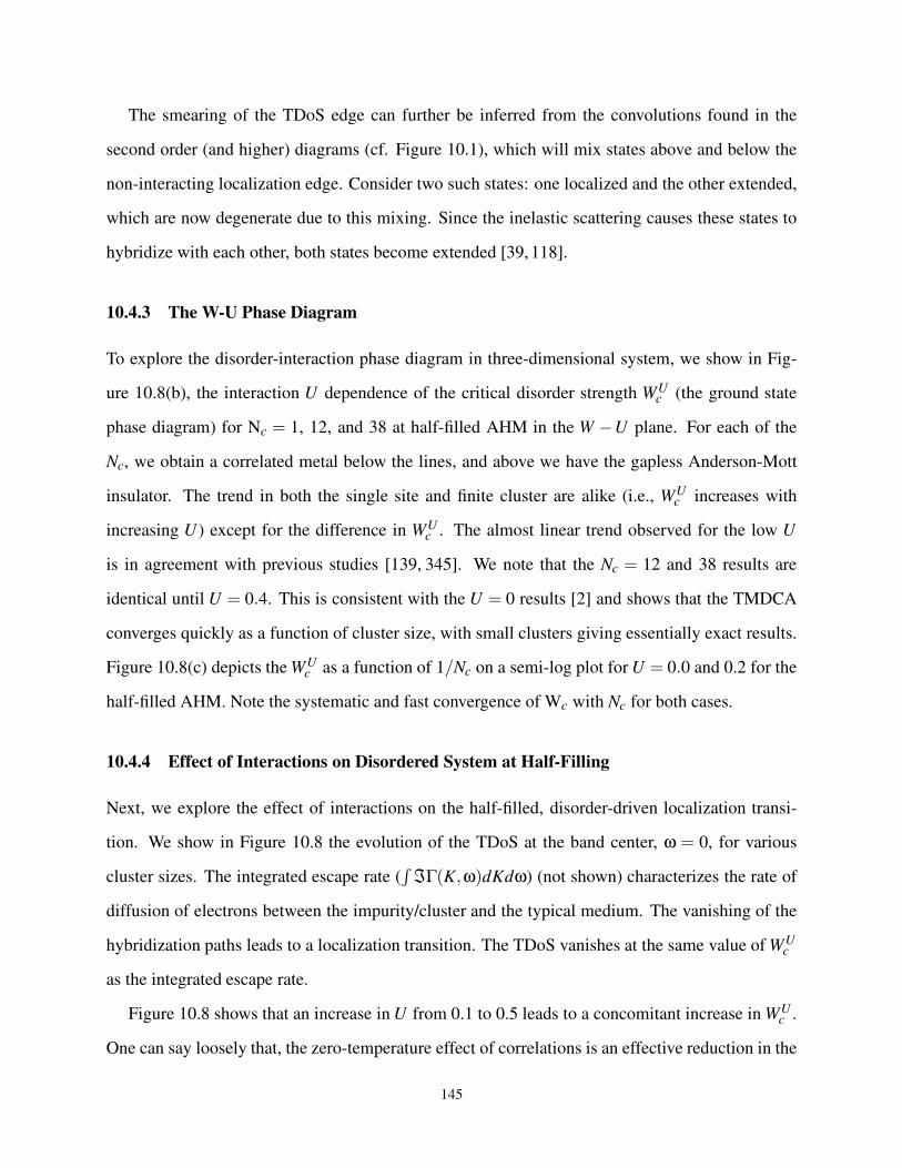
The smearing of the TDoS edge can further be inferred from the convolutions found in the
second order (and higher) diagrams (cf. Figure 10.1), which will mix states above and below the
non-interacting localization edge. Consider two such states: one localized and the other extended,
which are now degenerate due to this mixing. Since the inelastic scattering causes these states to
hybridize with each other, both states become extended [39, 118].
10.4.3 The W-U Phase Diagram
To explore the disorder-interaction phase diagram in three-dimensional system, we show in Fig-
ure 10.8(b), the interaction U dependence of the critical disorder strength WUc (the ground state
phase diagram) for Nc = 1, 12, and 38 at half-filled AHM in the W −U plane. For each of the
Nc, we obtain a correlated metal below the lines, and above we have the gapless Anderson-Mott
insulator. The trend in both the single site and finite cluster are alike (i.e., WUc increases with
increasing U ) except for the difference in WUc . The almost linear trend observed for the low U
is in agreement with previous studies [139, 345]. We note that the Nc = 12 and 38 results are
identical until U = 0.4. This is consistent with the U = 0 results [2] and shows that the TMDCA
converges quickly as a function of cluster size, with small clusters giving essentially exact results.
Figure 10.8(c) depicts the WUc as a function of 1/Nc on a semi-log plot for U = 0.0 and 0.2 for the
half-filled AHM. Note the systematic and fast convergence of Wc with Nc for both cases.
10.4.4 Effect of Interactions on Disordered System at Half-Filling
Next, we explore the effect of interactions on the half-filled, disorder-driven localization transi-
tion. We show in Figure 10.8 the evolution of the TDoS at the band center, ω = 0, for various
cluster sizes. The integrated escape rate (∫
ℑΓ(K,ω)dKdω) (not shown) characterizes the rate of
diffusion of electrons between the impurity/cluster and the typical medium. The vanishing of the
hybridization paths leads to a localization transition. The TDoS vanishes at the same value of WUc
as the integrated escape rate.
Figure 10.8 shows that an increase in U from 0.1 to 0.5 leads to a concomitant increase in WUc .
One can say loosely that, the zero-temperature effect of correlations is an effective reduction in the
145
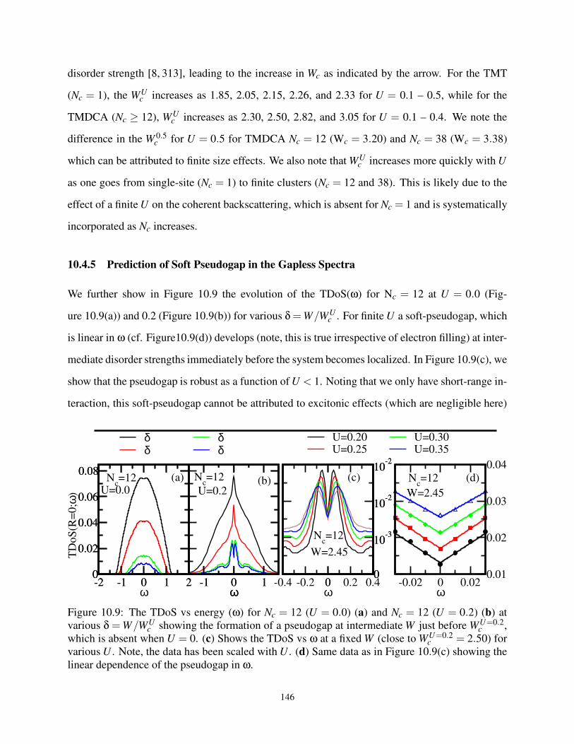
disorder strength [8, 313], leading to the increase in Wc as indicated by the arrow. For the TMT
(Nc = 1), the WUc increases as 1.85, 2.05, 2.15, 2.26, and 2.33 for U = 0.1 – 0.5, while for the
TMDCA (Nc ≥ 12), WUc increases as 2.30, 2.50, 2.82, and 3.05 for U = 0.1 – 0.4. We note the
difference in the W 0.5c for U = 0.5 for TMDCA Nc = 12 (Wc = 3.20) and Nc = 38 (Wc = 3.38)
which can be attributed to finite size effects. We also note that WUc increases more quickly with U
as one goes from single-site (Nc = 1) to finite clusters (Nc = 12 and 38). This is likely due to the
effect of a finite U on the coherent backscattering, which is absent for Nc = 1 and is systematically
incorporated as Nc increases.
10.4.5 Prediction of Soft Pseudogap in the Gapless Spectra
We further show in Figure 10.9 the evolution of the TDoS(ω) for Nc = 12 at U = 0.0 (Fig-
ure 10.9(a)) and 0.2 (Figure 10.9(b)) for various δ =W/WUc . For finite U a soft-pseudogap, which
is linear in ω (cf. Figure10.9(d)) develops (note, this is true irrespective of electron filling) at inter-
mediate disorder strengths immediately before the system becomes localized. In Figure 10.9(c), we
show that the pseudogap is robust as a function of U < 1. Noting that we only have short-range in-
teraction, this soft-pseudogap cannot be attributed to excitonic effects (which are negligible here)
-0.4 -0.2 0 0.2 0.4ω
0
10-3
10-2
10-2
U=0.20U=0.25
-2 -1 0 1 20
0.02
0.04
0.06
0.08
δ =0.80δ=0.88
-1 0 1ω
-1 0 1ω
δ=0.96δ=0.98
-2 -1 0 1 2ω
0
0.02
0.04
0.06
0.08
00
10-3
10-2
10-2
U=0.30U=0.35
-0.02 0 0.02ω
0.01
0.02
0.03
0.04
TD
oS
(R=
0;ω
)
Nc=12
U=0.2
Nc=12
U=0.0
W=2.45
(a) (b) (c)
Nc=12
(d)Nc=12
W=2.45
Figure 10.9: The TDoS vs energy (ω) for Nc = 12 (U = 0.0) (a) and Nc = 12 (U = 0.2) (b) at
various δ =W/WUc showing the formation of a pseudogap at intermediate W just before WU=0.2
c ,
which is absent when U = 0. (c) Shows the TDoS vs ω at a fixed W (close to WU=0.2c = 2.50) for
various U . Note, the data has been scaled with U . (d) Same data as in Figure 10.9(c) showing the
linear dependence of the pseudogap in ω.
146
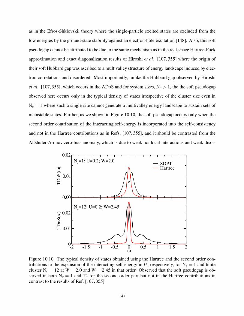
as in the Efros-Shklovskii theory where the single-particle excited states are excluded from the
low energies by the ground-state stability against an electron-hole excitation [148]. Also, this soft
pseudogap cannot be attributed to be due to the same mechanism as in the real-space Hartree-Fock
approximation and exact diagonalization results of Hiroshi et al. [107, 355] where the origin of
their soft Hubbard gap was ascribed to a multivalley structure of energy landscape induced by elec-
tron correlations and disordered. Most importantly, unlike the Hubbard gap observed by Hiroshi
et al. [107, 355], which occurs in the ADoS and for system sizes, Nc > 1, the the soft pseudogap
observed here occurs only in the typical density of states irrespective of the cluster size even in
Nc = 1 where such a single-site cannot generate a multivalley energy landscape to sustain sets of
metastable states. Further, as we shown in Figure 10.10, the soft pseudogap occurs only when the
second order contribution of the interacting self-energy is incorporated into the self-consistency
and not in the Hartree contributions as in Refs. [107, 355], and it should be contrasted from the
Altshuler-Aronov zero-bias anomaly, which is due to weak nonlocal interactions and weak disor-
0
0.01
0.02
TD
oS
(ω)
-2 -1.5 -1 -0.5 0 0.5 1 1.5 2ω
0
0.01
0.02
0.03
TD
oS
(ω)
SOPTHartree
Nc=12; U=0.2; W=2.45
Nc=1; U=0.2; W=2.0
Figure 10.10: The typical density of states obtained using the Hartree and the second order con-
tributions to the expansion of the interacting self-energy in U , respectively, for Nc = 1 and finite
cluster Nc = 12 at W = 2.0 and W = 2.45 in that order. Observed that the soft pseudogap is ob-
served in both Nc = 1 and 12 for the second order part but not in the Hartree contributions in
contrast to the results of Ref. [107, 355].
147
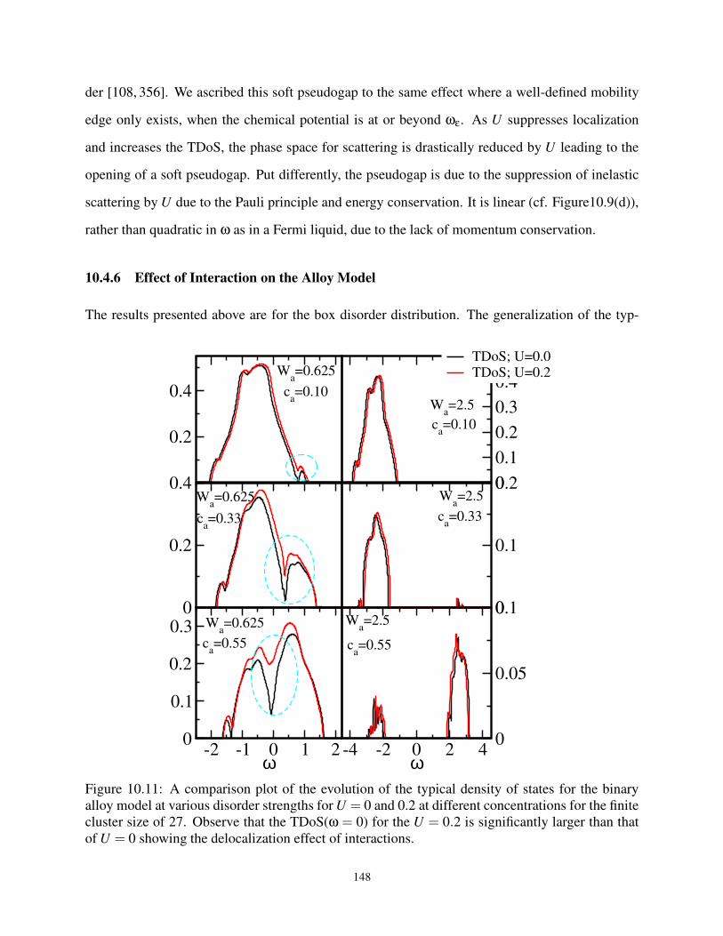
der [108, 356]. We ascribed this soft pseudogap to the same effect where a well-defined mobility
edge only exists, when the chemical potential is at or beyond ωε. As U suppresses localization
and increases the TDoS, the phase space for scattering is drastically reduced by U leading to the
opening of a soft pseudogap. Put differently, the pseudogap is due to the suppression of inelastic
scattering by U due to the Pauli principle and energy conservation. It is linear (cf. Figure10.9(d)),
rather than quadratic in ω as in a Fermi liquid, due to the lack of momentum conservation.
10.4.6 Effect of Interaction on the Alloy Model
The results presented above are for the box disorder distribution. The generalization of the typ-
0
0.2
0.4 0
0.1
0.2
0.3
0.4
0.5
0.2
0.4
TDoS; U=0.0TDoS; U=0.2
-2 -1 0 1 2ω
0
0.1
0.2
0.3
-4 -2 0 2 4ω
0
0.05
0.10
0.1
0.2
ca=0.33
ca=0.55
Wa=0.625
Wa=2.5
Wa=2.5
Wa=2.5
Wa=0.625
ca=0.10
Wa=0.625
ca=0.10
ca=0.33
ca=0.55
Figure 10.11: A comparison plot of the evolution of the typical density of states for the binary
alloy model at various disorder strengths for U = 0 and 0.2 at different concentrations for the finite
cluster size of 27. Observe that the TDoS(ω = 0) for the U = 0.2 is significantly larger than that
of U = 0 showing the delocalization effect of interactions.
148
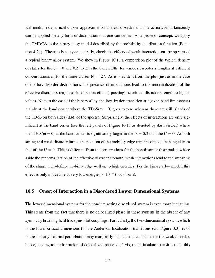
ical medium dynamical cluster approximation to treat disorder and interactions simultaneously
can be applied for any form of distribution that one can define. As a prove of concept, we apply
the TMDCA to the binary alloy model described by the probability distribution function (Equa-
tion 4.2d). The aim is to systematically, check the effects of weak interaction on the spectra of
a typical binary alloy system. We show in Figure 10.11 a comparison plot of the typical density
of states for the U = 0 and 0.2 (1/15th the bandwidth) for various disorder strengths at different
concentrations ca for the finite cluster Nc = 27. As it is evident from the plot, just as in the case
of the box disorder distributions, the presence of interactions lead to the renormalization of the
effective disorder strength (delocalization effects) pushing the critical disorder strength to higher
values. Note in the case of the binary alloy, the localization transition at a given band limit occurs
mainly at the band center where the TDoS(ω = 0) goes to zero whereas there are still islands of
the TDoS on both sides (±ω) of the spectra. Surprisingly, the effects of interactions are only sig-
nificant at the band center (see the left panels of Figure 10.11 as denoted by dash circles) where
the TDoS(ω = 0) at the band center is significantly larger in the U = 0.2 than the U = 0. At both
strong and weak disorder limits, the position of the mobility edge remains almost unchanged from
that of the U = 0. This is different from the observations for the box disorder distribution where
aside the renormalization of the effective disorder strength, weak interactions lead to the smearing
of the sharp, well-defined mobility edge well up to high energies. For the binary alloy model, this
effect is only noticeable at very low energies ∼ 10−4 (not shown).
10.5 Onset of Interaction in a Disordered Lower Dimensional Systems
The lower dimensional systems for the non-interacting disordered system is even more intriguing.
This stems from the fact that there is no delocalized phase in these systems in the absent of any
symmetry breaking field like spin-orbit couplings. Particularly, the two-dimensional system, which
is the lower critical dimensions for the Anderson localization transitions (cf. Figure 3.3), is of
interest as any external perturbation may marginally induce localized states for the weak disorder,
hence, leading to the formation of delocalized phase vis-à-vis, metal-insulator transitions. In this
149
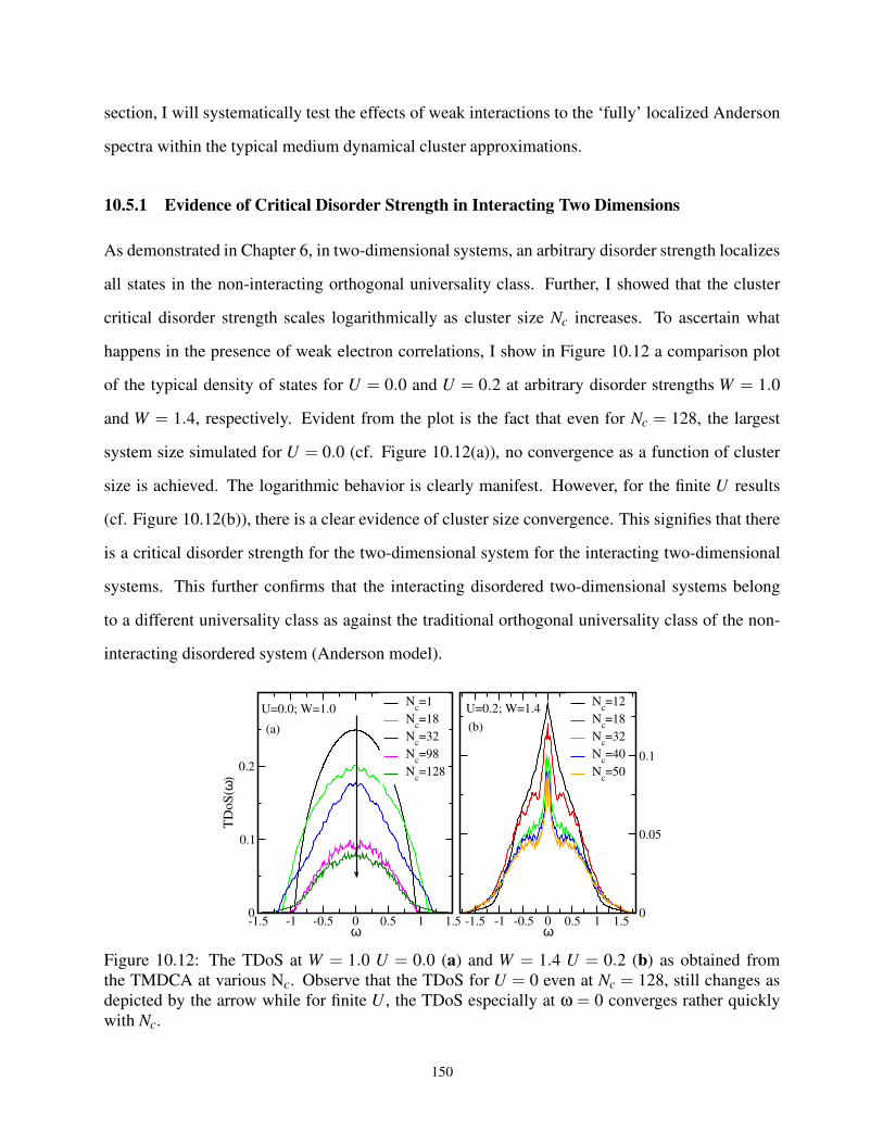
section, I will systematically test the effects of weak interactions to the ‘fully’ localized Anderson
spectra within the typical medium dynamical cluster approximations.
10.5.1 Evidence of Critical Disorder Strength in Interacting Two Dimensions
As demonstrated in Chapter 6, in two-dimensional systems, an arbitrary disorder strength localizes
all states in the non-interacting orthogonal universality class. Further, I showed that the cluster
critical disorder strength scales logarithmically as cluster size Nc increases. To ascertain what
happens in the presence of weak electron correlations, I show in Figure 10.12 a comparison plot
of the typical density of states for U = 0.0 and U = 0.2 at arbitrary disorder strengths W = 1.0
and W = 1.4, respectively. Evident from the plot is the fact that even for Nc = 128, the largest
system size simulated for U = 0.0 (cf. Figure 10.12(a)), no convergence as a function of cluster
size is achieved. The logarithmic behavior is clearly manifest. However, for the finite U results
(cf. Figure 10.12(b)), there is a clear evidence of cluster size convergence. This signifies that there
is a critical disorder strength for the two-dimensional system for the interacting two-dimensional
systems. This further confirms that the interacting disordered two-dimensional systems belong
to a different universality class as against the traditional orthogonal universality class of the non-
interacting disordered system (Anderson model).
-1.5 -1 -0.5 0 0.5 1 1.5ω
0
0.1
0.2
TD
oS
(ω)
Nc=1
Nc=18
Nc=32
Nc=98
Nc=128
-1.5 -1 -0.5 0 0.5 1 1.5ω
0
0.05
0.1
Nc=12
Nc=18
Nc=32
Nc=40
Nc=50
U=0.0; W=1.0 U=0.2; W=1.4
(a) (b)
Figure 10.12: The TDoS at W = 1.0 U = 0.0 (a) and W = 1.4 U = 0.2 (b) as obtained from
the TMDCA at various Nc. Observe that the TDoS for U = 0 even at Nc = 128, still changes as
depicted by the arrow while for finite U , the TDoS especially at ω = 0 converges rather quickly
with Nc.
150
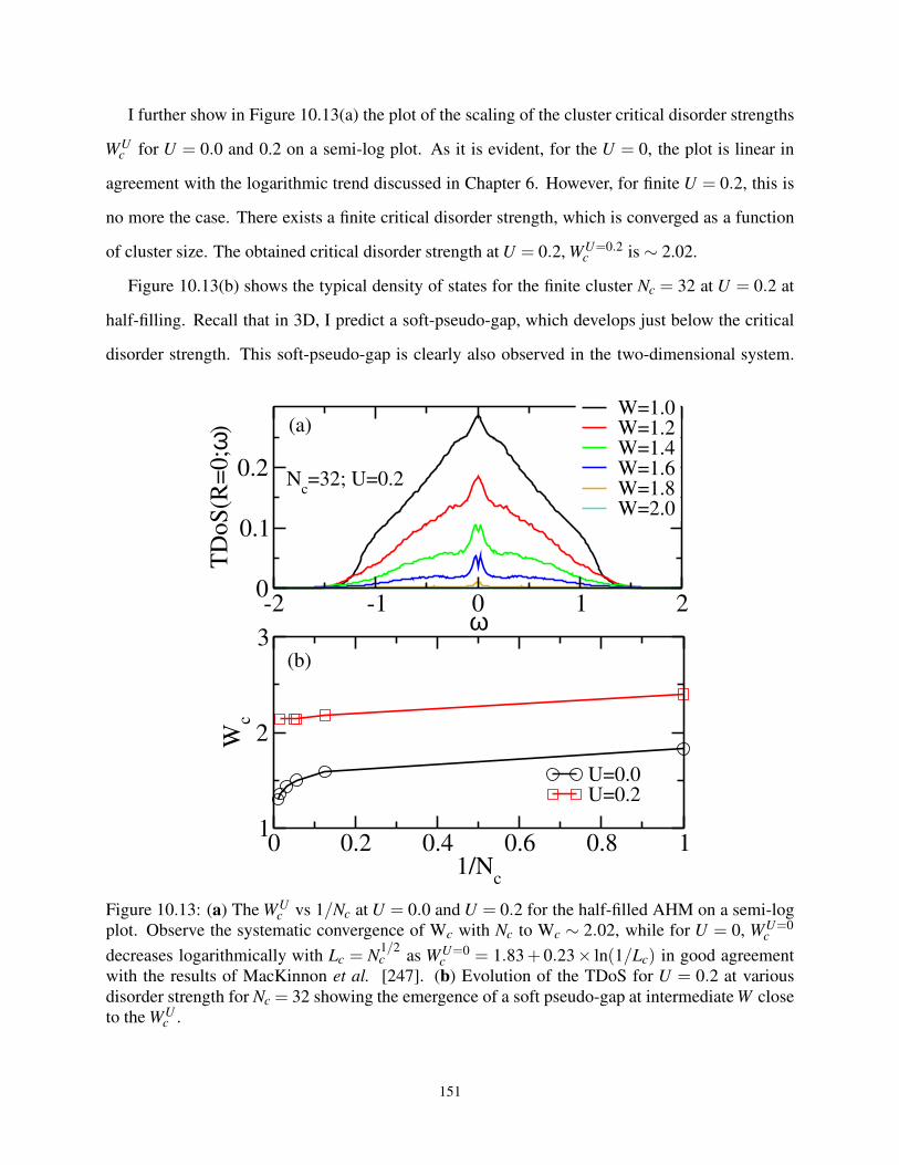
I further show in Figure 10.13(a) the plot of the scaling of the cluster critical disorder strengths
WUc for U = 0.0 and 0.2 on a semi-log plot. As it is evident, for the U = 0, the plot is linear in
agreement with the logarithmic trend discussed in Chapter 6. However, for finite U = 0.2, this is
no more the case. There exists a finite critical disorder strength, which is converged as a function
of cluster size. The obtained critical disorder strength at U = 0.2, WU=0.2c is ∼ 2.02.
Figure 10.13(b) shows the typical density of states for the finite cluster Nc = 32 at U = 0.2 at
half-filling. Recall that in 3D, I predict a soft-pseudo-gap, which develops just below the critical
disorder strength. This soft-pseudo-gap is clearly also observed in the two-dimensional system.
-2 -1 0 1 2ω
0
0.1
0.2
TD
oS
(R=
0;ω
)
W=1.0W=1.2W=1.4W=1.6W=1.8W=2.0
0 0.2 0.4 0.6 0.8 11/N
c
1
2
3
Wc
U=0.0U=0.2
Nc=32; U=0.2
(a)
(b)
Figure 10.13: (a) The WUc vs 1/Nc at U = 0.0 and U = 0.2 for the half-filled AHM on a semi-log
plot. Observe the systematic convergence of Wc with Nc to Wc ∼ 2.02, while for U = 0, WU=0c
decreases logarithmically with Lc = N1/2c as WU=0
c = 1.83+ 0.23× ln(1/Lc) in good agreement
with the results of MacKinnon et al. [247]. (b) Evolution of the TDoS for U = 0.2 at various
disorder strength for Nc = 32 showing the emergence of a soft pseudo-gap at intermediate W close
to the WUc .
151
As in the three-dimensional system, the soft-pseudo-gap only develops at finite U only in the
typical medium dynamical cluster approximation as it is not observed in the dynamical cluster
approximation even at finite electron-electron interactions.
10.6 Conclusions
Based on experiment, theory, and simulations, there is a growing consensus that the local density
of state in a disordered system develops a highly skewed [45], log-normal distribution [52, 140,
141] with a typical value given by the geometric mean that vanishes at the localization transition,
and hence, acts as the proper order parameter for the localization transitions. New mean field
theories for localization, including the typical medium theory and its cluster extension, the typical
medium dynamical cluster approximation have been proposed. The TMDCA is extended to weakly
interacting systems using second order perturbation theory. In three-dimensions, we find that weak
local interactions lead to increase in Wc, with the localization edge preserved when the chemical
potential is at or beyond the mobility edge energy. For finite U we observe a soft-pseudogap for
values of the disorder strength just above WUc . In two-dimensions, we recall that for the non-
interacting systems, the cluster size (same as conductivity) decreases logarithmically with disorder
strength. However, as shown in Section 10.5, this logarithmic behavior is replaced by an algebraic
trend for a weakly interacting disorder system achieving a convergence with the cluster size. This
implies that the interacting two-dimensional systems behaves more like a 3D system with a critical
disorder strength for e.g., U = 0.2, WU=0.2c ∼ 2.02. Also, the soft-pseudo gap observed in three-
dimensions is present in two-dimensions.
152
Chapter 11
Two-Particle Formalism within the Typical
Medium Dynamical Cluster Approximation
In this chapter, I will outline the steps in formulating a two-particle theory within the typical
medium dynamical cluster approximation and apply it to the calculation of the direct current con-
ductivity for various systems sizes as a function of increasing disorder strength using the box
disorder distribution.
11.1 Introduction
There is wealth of experimental transport data on strongly disordered systems that have defied ex-
planation by the conventional transport theory, which generally have been very successful in appli-
cations to good metals. Some attempts have been made to propose and/or develop a formalism for
extracting some information about the conductivity in the metal-insulator-transitions in disordered
electron systems, i.e., the incipient electron localization vis-à-vis the vanishing of the direct current
conductivity, which determines the mobility edge and the trajectories of the mobility edge. Based
on model-coupling ideas, Götze [357] develop a self-consistent localization formalism, which was
applied by Prelovsek [358] to calculate the conductivity for the non-interacting electron system.
An approach based on potential well analogy with the CPA was formulated [359–362] and used
to calculate the conductivity in various disorder distributions [359–364]. The diagrammatic self-
consistent approach of Vollhardt and Wöfle [259] was used to calculate conductivity for the An-
derson model [365–368], and other various models [359, 361, 369] including in the presence of
electron-electron interactions [370]. Aguair et al. [55] used the inverse of the typical density of
states as an approximation to the resistivity and showed that the resistivity curves as a function of
temperature is reminiscent of the Mooij correlations originally observed in disordered transition
153
metal alloys [371]. Girvin and Jonson [372] introduced an approximate scheme for calculating
conductivity that becomes accurate only close to the localization transition. This method was fur-
ther utilized by Dobrosavljevic et al. [105] in their study.
It is worthwhile to note and distinguish the method proposed here from other methods of calcu-
lating conductivity already well described in literature [36, 37, 44, 259, 357, 373]. In the traditional
formulation of the DMFA (or CPA) and its cluster extensions, the key ingredient in calculating
conductivity is the average medium self-energy and the average, fully dressed Green function [36].
While this approach is robust in obtaining conductivity, it is important to note that it cannot charac-
terize electron localization. This follows from the problems already well discussed in the previous
Chapters due to the fact that the fluctuations of the local average Green function, which is an in-
put in the calculation of the conductivity is so large that its typical value is far removed from the
average one [374]. Thus, the local average Green function, which characterizes these mean-field
environments does not have any information about the typical nature of the local order parameter
needed to signal a phase transition. Further, the method proposed here treats the localized and
extended spectra separately such that the two-particle correlation function has the information of
both the localized and the extended part.
11.2 Pedagogical Concepts: Local Mean-field and Cluster Extensions
The dynamical mean-field approximation (DMFA) or its equivalent, coherent potential approxima-
tion (CPA) remains one of the most used methods for solving interacting and disordered systems,
respectively. They are mean-field approaches, which are exact in infinite dimensions [375–378].
Since they are local approximations, spatial correlations are neglected while retaining local dynam-
ical correlations. To incorporate nonlocal correlations in finite dimensions, the dynamical cluster
approximation (DCA) [263,308] remains one of the best cluster extensions of choice. As has been
demonstrated, the DCA is motivated by the DMFA based on the coarse-graining of the propagators
used in the construction of the generating functional and its derivatives over the entire Brillouin
zone [263, 308]. However in the DCA, the momentum independent quantities as in the DMFA or
154
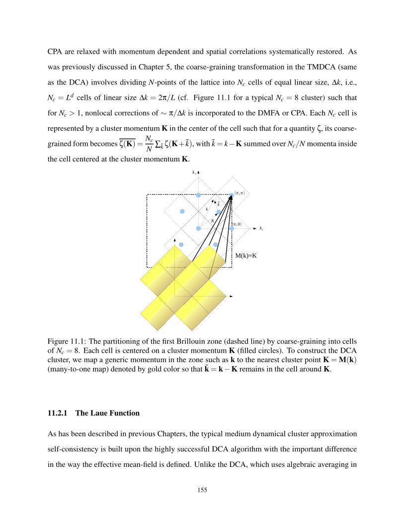
CPA are relaxed with momentum dependent and spatial correlations systematically restored. As
was previously discussed in Chapter 5, the coarse-graining transformation in the TMDCA (same
as the DCA) involves dividing N-points of the lattice into Nc cells of equal linear size, ∆k, i.e.,
Nc = Ld cells of linear size ∆k = 2π/L (cf. Figure 11.1 for a typical Nc = 8 cluster) such that
for Nc > 1, nonlocal corrections of ∼ π/∆k is incorporated to the DMFA or CPA. Each Nc cell is
represented by a cluster momentum K in the center of the cell such that for a quantity ζ, its coarse-
grained form becomes ζ(K) =Nc
N∑k ζ(K+ k), with k = k−K summed over Nc/N momenta inside
the cell centered at the cluster momentum K.
Figure 11.1: The partitioning of the first Brillouin zone (dashed line) by coarse-graining into cells
of Nc = 8. Each cell is centered on a cluster momentum K (filled circles). To construct the DCA
cluster, we map a generic momentum in the zone such as k to the nearest cluster point K = M(k)(many-to-one map) denoted by gold color so that k = k−K remains in the cell around K.
11.2.1 The Laue Function
As has been described in previous Chapters, the typical medium dynamical cluster approximation
self-consistency is built upon the highly successful DCA algorithm with the important difference
in the way the effective mean-field is defined. Unlike the DCA, which uses algebraic averaging in
155
the self-consistent, the TMDCA environment uses typical averaging. Hence, all the discussions of
the development of a two-particle formalism for the TMDCA will overlap with the well established
two-particle formalism of the DCA. As demonstrated by Müller-Hartmann [218], coarse-graining,
as is done in the DCA, becomes exact in the limit of infinite dimensions (d → ∞). An important
property that becomes vital in formulating cluster extensions of the DMFA same as the CPA is the
Laue function. For a typical Hubbard-like model, the Laue function ∆
∆(k1,k2,k3,k4) = ∑r
exp [ir · (k1+k2 −k3 −k4)] = Nδk1+k2,k3+k4(11.1)
implicitly characterizes the bare vertex, which expresses the momentum conservation k1 and k3
(k2 and k4) entering (leaving) each vertex. Here, k1 and k2 (k3 and k4) are the momenta entering
(leaving) each vertex through the legs of G.
Following the microscopic diagrammatic derivation of the DCA [308], the systematic restora-
tion of momentum conservation at the internal vertices, which is neglected in single site approaches
require that momentum conservation be (partially) guaranteed between the cells and neglected
within a cell. Taking into account the cluster and cell momenta so that ki = Ki + ki, i = 1,4, then
Equation 11.1 becomes
∆(k1,k2,k3,k4) = ∑r
ei(k1−k2+k3−k4+K1−K2+K3−K4)·r (11.2)
= Nc ∑n
1
n!
((k1 − k2 + k3 − k4) ·∆K1
)nδK1+K3,K2+K4
Within the TMDCA, only the n = 0 (first) term of Equation 11.2 is kept [263] so that
∆T MDCA(k1,k2,k3,k4) = NcδM(k1)+M(k3),M(k2)+M(k4) = ∆(k1,k2,k3,k4)+O(∆k) , (11.3)
where M(k) is a function which maps k onto the momentum label K of the cell containing k
(many-to-one map) (see, Figure 11.1). This choice for the Laue function guarantees the system-
atic restoration at the internal vertices in the TMDCA and interpolates between the exact result,
Equation 11.1, which it recovers when Nc → N and the single site result, Equation 11.4, which it
156
recovers when Nc = 1. With this choice of the Laue function, the momenta of each internal Green
function leg may be freely summed over the cell, i.e., each internal Green function leg G(k1,ω)
in the diagram is replaced by G(M(k1),ω). Note in the limit of infinite dimension d → ∞, Equa-
tion 11.1 reduces to [218]
∆d→∞(k1,k2,k3,k4) = 1+O(1/d) . (11.4)
11.3 Free Energy and Two-Particle Quantities
The microscopic derivation of the DCA based on the diagrammatic expression of the grand poten-
tial enables us to access thermodynamic properties. Motivated by this, we use the free energy to
construct a unique platform to gain access into the local order parameter of a disordered system.
Let us take the simplest order parameter, the magnetization, m, which is the trace of the local Green
function. The susceptibility follows immediately as the second derivative, and we end up with a
Bethe-Salpeter equation. An order parameter within the TMDCA can intuitively be motivated
by the above physical concept. The key task then will be how to formulate an appropriate order
parameter in the TMDCA, which is a K-space formalism. We will try to answer this important
question below.
Baym and Kadanoff [379, 380] demonstrated that a thermodynamically consistent approxima-
tion may be formulated by requiring that the self-energy Σ be the functional derivative of the
Baym-Kadanoff generation function Φ with respect to the Green function, i.e., fulfill
G−1 −G−1 = Σ =δΦ[G]
δG. (11.5)
This should be done self-consistently by carefully summing over all closed, connected, and com-
pact graphs constructed from the fully dressed Green function G. With this, the irreducible ver-
tices Γ = δΣ/δG. The second order contribution to the generating functional Φ for a Hubbard-like
model is as depicted in Figure 11.2(a), becomes a functional of the local interaction and the Green
function. In obtaining the self-energy Σ from a functional derivative of Φ with respect to the Green
157

Figure 11.2: (a) The second order contribution to the generating functional Φ for the DMFA. As
we apply the DMFA coarse-graining approximation, Equation 11.4, Φ becomes a functional of
the fully dressed local Green function. (b) The second-order term in Φ for a Hubbard-like model.
Here the undulating line represents the interaction U , and on the LHS (RHS) the solid line is the
lattice (coarse-grained) single-particle Green functions. When the TMDCA Laue function is used
to describe momentum conservation at the internal vertices, the momenta collapse onto the cluster
momenta with each lattice Green function now replaced by the corresponding coarse-grained ones.
function G, one of the Green function lines is effectively broken. With the appropriate set of Dyson
and Bethe-Salpeter equations, and the diagrammatic form of the generating functional, a complete
diagrammatic formalism for accessing thermodynamic quantities can be formulated.
As demonstrated in the DCA, the unique choice of the self-energy, which guarantees that the
DCA free energy is appropriately minimized is the mapping Σ(k,ω) = Σ(M(k),ω). Motivated
by this, care must also be taken in constructing two-particle quantities. Following Ref. [263],
the appropriate definition of the irreducible vertice between the lattice and the cluster should be
ΓΓΓ ≈ ΓΓΓ = δΣΣΣ/δG yields an estimate for the susceptibility, which is equivalent to the result of the
second derivative of the free energy with respect to an external field as will be demonstrated shortly.
With this mind, the cluster calculations should be used to provide irreducible quantities and to-
gether with the bare real-lattice Green functions, one may construct the corresponding reducible
quantities [263]. This prescription is not only motivated physically for the single-particle Green
functions but can be shown to be the same for the two-particle counterparts [263].
158
11.3.1 Derivability of the Generating Function
The generating functional Φ can also be coarse-grained. The generating functional is the sum over
all the closed, connected, compact diagrams, such as the one shown in Figure 11.2(b) given as
Φ(G) = ∑l
pltr[
ΣlG]
(11.6)
The trace denotes summation over frequency, momentum, and spin, Σl is a set of irreducible self-
energy diagrams of the lth order in interaction, G is the fully dressed Green function related to Σ via
the Dyson equation (11.5), pl is a counting factor, which measures the number of occurrences of
G in each term (for a Hubbard-like model, pl = 1/l). From Equation 11.9, it follows immediately
that Equation 11.5 is satisfied, as required for a “Φ-derivable” theory [267].
Intuitively, the choice of the Laue function for the TMDCA ∆T MDCA is the replacement of the
lattice quantities with their corresponding coarse-grained counterparts denoted with overbars (cf.
Figure 11.2(b)). For instance, the lattice Green function Gσ is replaced by the coarse-grained
cluster Green function Gσ. In the coarse-grained form, the external momentum label (k) of the
cluster self-energy in principle, is still the lattice momentum but the self-energy now only depends
on k through the function M(k). With the application of the Laue function on the vertices, the
corresponding TMDCA Φ functional is
ΦT MDCA [G] = ∑l
pltr[
ΣlG]
(11.7)
with the corresponding lattice quantities,
δΦT MDCA
δG= Σ =
δΦT MDCA
δG(11.8)
The second equality is true since the variation δ/δG corresponds to cutting a Green function line.
The relation between the grand potential functional (here the free energy FT MDCA) and the gener-
ating functional Φ may be expressed in terms of the linked cluster expansion [381] as
FT MDCA =−kBT (Φ[G]− tr [ΣG]− tr ln [−G]) (11.9)
159
where the trace depicts a summation over cluster sites X, superlattice wavevectors k, frequency,
and spin [267]. Rearranging and taking functional derivative we obtain
− 1
κT
δFT MDCA
δG(~k)=
δΣc
δG(~k)−Tr
δ [ΣG]
δG(~k)+Tr
1
G(~k). (11.10)
The perturbative series for Φ, Σ, and the irreducible vertices Γ in the DMFA are identical to those
of the corresponding impurity model, hence, conventional impurity solvers may be used. However,
care must be taken to avoid overcounting by excluding the local self-energy Σ(ω)
G(ω)−1 = G(ω)−1 +Σ(ω) (11.11)
from the local propagator G input to the impurity solver. This is important since most impurity
solvers will sum all the diagrams equally, not just the skeletal ones. Here, G(ω) is the fully dressed
local Green function. In this local approximation regime, the Hubbard model has the same dia-
grammatic expansion as the Anderson impurity model.
From Eqs. 11.9 and 11.10, observe that FT MDCA is stationary with respect to G when
−1
kBT
δFT MDCA
δG(k)= Σ(M(k))−Σ(k) = 0, (11.12)
which implies that Σ(k) = Σ(M(k)) is the proper approximation for the lattice self-energy corre-
sponding to ΦT MDCA. The corresponding lattice single-particle propagator is then given by
G(k,ω) =1
ω− εk − ε− Σ(M(k),ω). (11.13)
where k = K + k. From the above formulation, it is obvious that the observables calculated from
the Green function G agree with those calculated from the free energy functional, i.e., thermody-
namically consistent. Since momentum and energy are conserved in the vertices, together with
condition (11.5) ensures that conservation laws e.g., Ward identities are satisfied [380]. A similar
procedure can be used to construct the two-particle quantities needed for calculating the conductiv-
ity or the nature of the phase diagram within the typical medium dynamical cluster approximation.
160
This procedure is a generalization of the response functions calculations as in single impurity
solvers [382, 383].
Within the TMDCA, spatial correlations, which are important ingredient for enhancing coher-
ent backscattering, quantum tunneling vis-á-vis deep trapped states, etc will allow for the proper
characterization of electron localization. To be able to characterize electron localization using the
direct current (DC) conductivity, we have to be able to compute response functions, which ther-
modynamically, are generally defined as second derivatives of the free energy with respect to some
external fields. The quantities ΦT MDCA(G), Σ, and FT MDCA depend on these fields only through G
and the bare G . Following Baym and Kadanoff [379], the approximation for Γ can be written as
Γ ≈ Γ ≡ δΣ
δG(11.14)
which is the same as that obtained from the second derivative of FT MDCA with respect to the applied
field. For instance, assuming an external homogeneous field h with spin σ, the magnetization, m is
m = Tr [σGσ] . (11.15)
and the susceptibility, which is the second derivative follows immediately as,
∂m
∂h= Tr
[
σ∂Gσ
∂h
]
. (11.16)
Recall that Gσ =(G0−1
σ − Σσ
)−1. Then, using this in Equation 11.16, we obtain,
∂m
∂h= Tr
[
σ∂Gσ
∂h
]
= Tr
[
G2σ
(
1+σ∂Σσ
∂Gσ′
∂Gσ′
∂h
)]
. (11.17)
If we identify χσ,σ′ = σ∂Gσ′
∂h, and χ0
σ = G2σ, collect like terms within both traces, and sum over the
cell momenta k, we obtain the two-particle Dyson’s equation
2(χσ,σ − χσ,−σ
)= 2χ0
σ +2χ0σ
(Γσ,σ − Γσ,−σ
)(χσ,σ − χσ,−σ) . (11.18)
161
11.4 Calculation of Experimental Measurable Physical Quantities
So far, the formalisms that have been discussed above cannot be measured directly by experiment.
All measurable physical quantities can be expressed theoretically as either reducible one or two-
particle quantity. Both either the reducible one or two-particle parameters can be informed from
the Green function, which generally is the end product of a self-consistent, converged simula-
tion. For instance, to compare with experimental angle-resolved photoemission spectroscopy, the
single-particle Green function is the needed input, which is obtained directly by solving the Dyson
equation, self-consistently. For the calculation of the conductivity, the important input quantity is
the irreducible vertices in the different scattering channels obtained by solving the Bethe-Salpeter
equations for the lattice. Here, we will try to provide the details of how to obtain the two-particle
Green function and the mapping between the lattice and cluster, counterparts.
11.4.1 Particle-hole channel
In the particle-hole channel, the two-particle Green function (neglecting spin) is
χ(q,k,k′) =∫ β
0
∫ β
0
∫ β
0
∫ β
0dτ1dτ2dτ3dτ4 × ei((ωn+ν)τ1−ωnτ2+ωn′τ3−(ωn′+ν)τ4) (11.19)
× 〈Tτc†k+q(τ1)ck(τ2)c
†k′(τ3)ck′+q(τ4)〉.
Here, we use the conventional notations k = (k, iωn), k′ = (k,ω′n) and q= (q,νn) [381], where Tτ is
the time ordering operator. The two-particle irreducible vertex Γσ,σ′(q,k,k′), which is the analogue
of the self-energy and χσ,σ′(q,k,k′), which is the non-interacting susceptibility constructed from a
pair of fully-dressed single-particle Green functions are related to each other via the Bethe-Salpeter
equation (Figure 11.3):
χ(q,k,k′) = χ0(q,k,k′)+χ0(q,k,k′′)×Γ(q,k′′,k′′′)χ(q,k′′′,k′) (11.20)
where the summation is for repeated indices. Applying many-to-one map, i.e., Γ(q,k,k′) →
Γc (q,M(k),M(k′)) (frequency labels have been suppressed) as in the TMDCA and substituting
162
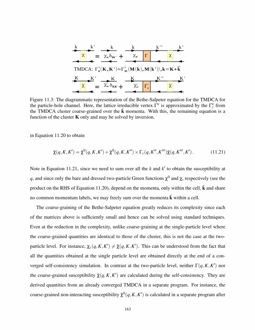
Figure 11.3: The diagrammatic representation of the Bethe-Salpeter equation for the TMDCA for
the particle-hole channel. Here, the lattice irreducible vertex Γν is approximated by the Γνc from
the TMDCA cluster coarse-grained over the k momenta. With this, the remaining equation is a
function of the cluster K only and may be solved by inversion.
in Equation 11.20 to obtain
χ(q,K,K′) = χ0(q,K,K′)+ χ0(q,K,K′′)×Γc(q,K′′,K′′′)χ(q,K′′′,K′) . (11.21)
Note in Equation 11.21, since we need to sum over all the k and k′ to obtain the susceptibility at
q, and since only the bare and dressed two-particle Green functions χ0 and χ, respectively (see the
product on the RHS of Equation 11.20), depend on the momenta, only within the cell, k and share
no common momentum labels, we may freely sum over the momenta k within a cell.
The coarse-graining of the Bethe-Salpeter equation greatly reduces its complexity since each
of the matrices above is sufficiently small and hence can be solved using standard techniques.
Even at the reduction in the complexity, unlike coarse-graining at the single-particle level where
the coarse-grained quantities are identical to those of the cluster, this is not the case at the two-
particle level. For instance, χc(q,K,K′) 6= χ(q,K,K′). This can be understood from the fact that
all the quantities obtained at the single particle level are obtained directly at the end of a con-
verged self-consistency simulation. In contrast at the two-particle level, neither Γ(q,K,K′) nor
the coarse-grained susceptibility χ(q,K,K′) are calculated during the self-consistency. They are
derived quantities from an already converged TMDCA in a separate program. For instance, the
coarse-grained non-interacting susceptibility χ0(q,K,K′) is calculated in a separate program after
163
the TMDCA converges using the relation
χ0[(q,ν);(K,ω);(K′,ω′)] = δK,K′δω,ω′Nc
N∑k
G(K+ k,ω)G(K+ k+q,ω+ν) (11.22)
and the corresponding cluster susceptibility is calculated by the cluster solver and the vertex func-
tion is obtained by solving the cluster two-particle Bethe-Salpeter equation
χc(q,K,K′) = χc0(q,K,K′)+χc
0(q,K,K′′)×Γc(q,K′′,K′′′)χc(q,K
′′′,K′). (11.23)
Combining Eqs. 11.21 and 11.23, then, we obtain the coarse-grained susceptibility as
χ−1 = χ−1c −χ0−1
c + χ0−1
, (11.24)
where, for example, χ is the matrix formed from χ(q,K,K′) for fixed q, which for our case q = 0.
11.4.2 Particle-particle channel
In the particle-particle channel, the calculation of susceptibilities is identical to the above that
of the particle-hole channel, except when the susceptibility calculations are done for transitions
to states of lower symmetry than the lattice symmetry. For instance, in order to obtain the pair
function of the desired symmetry (s, p,d), the two-particle Green function must be multiplied by
the corresponding form factors g(k) and g(k′) such that g(k)= 1 (s wave), g(k)= cos(kx)+cos(ky)
(extended s wave) and g(k) = cos(kx)−cos(ky) (dx2−y2 wave). Hence, the Bethe-Salpeter equation
becomes
g(k)χ(q,k,k′)g(k′) = g(k)χ0(q,k,k′)g(k′)+g(k)χ0(q,k,k′′) (11.25)
× Γ(q,k′′,k′′′)×χ(q,k′′′,k′)g(k′) .
where χ(q,k,k′) is the same as in Equation 11.19. Evaluating Equation 11.25 is not trivial if it is
to be coarse-grained, since this will partially convolve χ(q,k,k′) with two factors of g on the LHS
and one factor on the RHS. Hence for the susceptibilities, or any situation where the system has
164
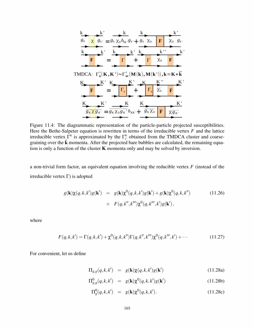
Figure 11.4: The diagrammatic representation of the particle-particle projected susceptibilities.
Here the Bethe-Salpeter equation is rewritten in terms of the irreducible vertex F and the lattice
irreducible vertex Γν is approximated by the Γνc obtained from the TMDCA cluster and coarse-
graining over the k momenta. After the projected bare bubbles are calculated, the remaining equa-
tion is only a function of the cluster K momenta only and may be solved by inversion.
a non-trivial form factor, an equivalent equation involving the reducible vertex F (instead of the
irreducible vertex Γ) is adopted
g(k)χ(q,k,k′)g(k′) = g(k)χ0(q,k,k′)g(k′)+g(k)χ0(q,k,k′′) (11.26)
× F(q,k′′,k′′′)χ0(q,k′′′,k′)g(k′) ,
where
F(q,k,k′) = Γ(q,k,k′)+χ0(q,k,k′′)Γ(q,k′′,k′′′)χ0(q,k′′′,k′)+ · · · (11.27)
For convenient, let us define
Πg,g(q,k,k′) = g(k)χ(q,k,k′)g(k′) (11.28a)
Π0g,g(q,k,k
′) = g(k)χ0(q,k,k′)g(k′) (11.28b)
Π0g(q,k,k
′) = g(k)χ0(q,k,k′) . (11.28c)
165
From here onward, the steps in the calculation of the two-particle quantities are identical to the
particle-hole channel: We invert the cluster particle-particle Bethe-Salpeter equation with g = 1
for the cluster and extract Γc. Then, we coarse-grain Equation 11.27 and use Γc to calculate the
coarse-grained F = Γc
(1− χ0Γc
)−1. Next, we coarse-grain Equation 11.26 and use the coarse-
grained F to calculate the coarse-grained Πg,g as
Πg,g(q,K,K′) = Π0g,g(q,K,K′)+ Π0
g(q,K,K′′)F(q,K′′,K′′′)Π0g(q,K
′′′,K′) . (11.29)
11.5 Calculating Conductivity in the Typical Medium DCA
We will in this section combine all the ideas developed in previous sections above to formulate
a method for calculating direct current (DC) conductivity within the typical medium dynamical
cluster approximation (TMDCA). In obtaining Πg,g (cf. Equation 11.29), recall that we coarse-
grained Equation 11.26, using the coarse-grained F . Below, we outline the steps involved as
Πg,g(q,K,K′) = g(k)χ(q,k,k′)g(k′) (11.30)
= g(k)χ0(q,k,k′)g(k′)× Γg,g(q,K′′,K′′′)
(
1−χ0gΓg,g
)−1
(q,K′′′,K′′′′)
χ0g(q,K
′′′′,k′)g(k′)
which, reduces to
Πg,g(q,K,K′) = Π0g,g(q,K,K′)+ Π0
g(q,K,K′′)F(q,K′′,K′′′)Π0g(q,K
′′′,K′) . (11.31)
In order to find the bare bubbles, we need the time-ordered lattice Green function (note k =
(k,ω)) Gl(q,k,k′,ω)
Gl(q,k,k′,ω) =
Gloc(q,K)δK,K′, if |ω|> ωe
Gext(q,k)δk,k′, if |ω|< ωe
(11.32)
where Gloc is the localized (only on the cluster) part of the Green function, Gext is the extended
part of the Green function, and ωe is the mobility edge energy.
166
For the non-interacting Anderson model, the scattering is purely classical, so the momentum
can change by a scattering event, but the frequency does not change. This implies that if the
external labels are ω and ω+ν, then, the lines will have these same labels, as such, requiring no
internal frequency integration. However, if the system is an interacting disordered, a distinction
needs to be made between elastic and inelastic scattering contributions. This is important since
interactions will induce inelastic scattering processes.
Considering Π0g,g(k,k
′), and using q = 0, then from above, recall that
Π0g,g(K,K′) = g(k)χ0(k,k′)g(k′). (11.33)
Then,
limν→0+
Π0g,g(K,K′,ω+ν) = δk,k′
Nc
N∑kk′
ϑK+k,xGloc(K,ω)ϑK+k′,xGloc(K,ω+ν)Θ(|ω|−ωe)
+ δk,k′Nc
N∑k
(ϑk+k,x)2Gext(K + k,ω)Gext(K+ k,ω+ν)Θ(ωe −|ω|)
(11.34a)
which, reduces to
limν→0+
Π0g,g(K,ω+ν) =
Nc
N
(
∑k
ϑK+k,x
)2
Gloc(K,ω)Gloc(K,ω+ν)Θ(|ω|−ωe) (11.34b)
+Nc
N∑k
(ϑk+k,x)2Gext(K+ k,ω)Gext(K + k,ω+ν)Θ(ωe −|ω|)
where Θ(x) is a step function. Similarly, Π0g(q,K,K′′) and Π0
g(q,K′′′,K′) from Equation 11.31 can
be expressed as
limν→0+
Π0g(K,ω+ν) =
Nc
N ∑k ϑK+k,xGloc(K,ω)Gloc(K,ω+ν), if |ω|> ωe
Nc
N ∑k ϑK+k,xGext(K + k,ω)Gext(K+ k,ω+ν), if |ω|6 ωe.
(11.35)
167
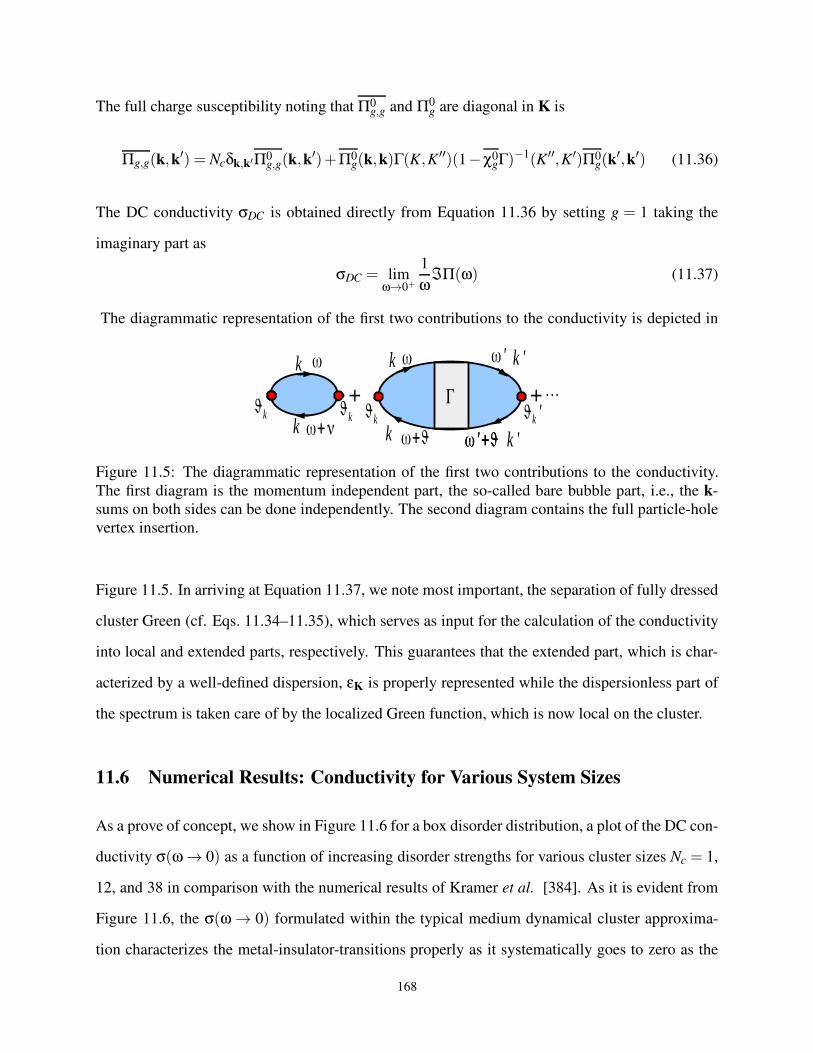
The full charge susceptibility noting that Π0g,g and Π0
g are diagonal in K is
Πg,g(k,k′) = Ncδk,k′Π0
g,g(k,k′)+Π0
g(k,k)Γ(K,K′′)(1−χ0gΓ)−1(K′′,K′)Π0
g(k′,k′) (11.36)
The DC conductivity σDC is obtained directly from Equation 11.36 by setting g = 1 taking the
imaginary part as
σDC = limω→0+
1
ωℑΠ(ω) (11.37)
The diagrammatic representation of the first two contributions to the conductivity is depicted in
Figure 11.5: The diagrammatic representation of the first two contributions to the conductivity.
The first diagram is the momentum independent part, the so-called bare bubble part, i.e., the k-
sums on both sides can be done independently. The second diagram contains the full particle-hole
vertex insertion.
Figure 11.5. In arriving at Equation 11.37, we note most important, the separation of fully dressed
cluster Green (cf. Eqs. 11.34–11.35), which serves as input for the calculation of the conductivity
into local and extended parts, respectively. This guarantees that the extended part, which is char-
acterized by a well-defined dispersion, εK is properly represented while the dispersionless part of
the spectrum is taken care of by the localized Green function, which is now local on the cluster.
11.6 Numerical Results: Conductivity for Various System Sizes
As a prove of concept, we show in Figure 11.6 for a box disorder distribution, a plot of the DC con-
ductivity σ(ω → 0) as a function of increasing disorder strengths for various cluster sizes Nc = 1,
12, and 38 in comparison with the numerical results of Kramer et al. [384]. As it is evident from
Figure 11.6, the σ(ω → 0) formulated within the typical medium dynamical cluster approxima-
tion characterizes the metal-insulator-transitions properly as it systematically goes to zero as the
168
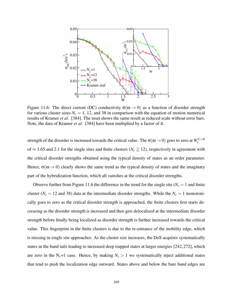
0 0.5 1 1.5 2 2.5 3W
0
0.01
0.02
0.03
0.04
0.05
σ DC(h_
/e2
)N
c=1
Nc=12
Nc=38
Kramer etal
1.5 2W
0
0.01
0.02
0.03
σ D.C
(h_/e
2)
Figure 11.6: The direct current (DC) conductivity σ(ω → 0) as a function of disorder strength
for various cluster sizes Nc = 1, 12, and 38 in comparison with the equation of motion numerical
results of Kramer et al. [384]. The inset shows the same result at reduced scale without error bars.
Note, the data of Kramer et al. [384] have been multiplied by a factor of π.
strength of the disorder is increased towards the critical value. The σ(ω→ 0) goes to zero at WU=0c
of ≈ 1.65 and 2.1 for the single sites and finite clusters (Nc ≧ 12), respectively in agreement with
the critical disorder strengths obtained using the typical density of states as an order parameter.
Hence, σ(ω → 0) clearly shows the same trend as the typical density of states and the imaginary
part of the hybridization function, which all vanishes at the critical disorder strengths.
Observe further from Figure 11.6 the difference in the trend for the single site (Nc = 1 and finite
cluster (Nc = 12 and 38) data at the intermediate disorder strengths. While the Nc = 1 monotoni-
cally goes to zero as the critical disorder strength is approached, the finite clusters first starts de-
creasing as the disorder strength is increased and then gets delocalized at the intermediate disorder
strength before finally being localized as disorder strength is further increased towards the critical
value. This fingerprint in the finite clusters is due to the re-entrance of the mobility edge, which
is missing in single site approaches. As the cluster size increases, the DoS acquires systematically
states in the band tails leading to increased deep trapped states at larger energies [242,272], which
are zero in the Nc=1 case. Hence, by making Nc > 1 we systematically inject additional states
that tend to push the localization edge outward. States above and below the bare band edges are
169
initially localized in deeply trapped states. They become delocalized with increasing W due to the
increasing DoS and hence increasing quantum tunneling between the deeply trapped states. They
finally become localized again with increasing disorder, which explains the re-entrant behavior.
There is lack of numerical data on the calculation of conductivity of disordered electron systems
leading to localization transitions. To benchmark our results, we compare our TMDCA results with
the numerical data of Kramer et al. [384]. Surprisingly, as a function of increase in cluster size, we
reproduce the essential features of their data. The present result is remarkable as this will enable
comparison with experimental results for electron localization since it is easier to measure σ(ω →
0) in experimental setting than any other order parameters characterizing localization transitions.
We believe that this will motivate experiments to measure σ(ω → 0) as a function of disorder
strength, which can be controlled by doping the ‘pure’ system with varying concentrations of the
dopant.
11.7 Conclusion
A two-particle formalism within the typical medium dynamical cluster approximation for calcu-
lating two-particle quantities like the conductivity are proposed. By carefully separating the Green
function into extended and localized parts, it is shown that this is the appropriate way of think-
ing about two-particle quantities for characterizing electron localization. As a function of disorder
strength, the direct conductivity σ(ω→ 0) calculated within the TMDCA is shown to be the appro-
priate two-particle order parameter characterizing the localization transitions. It is our hope that
this result will spurn both numerical calculations and experimental measurements of σ(ω → 0).
170
Bibliography
[1] C. E. Ekuma et al.. J. Phys. Conden. Matt. 26(27), 274209 (2014).
[2] C. E. Ekuma et al.. Phys. Rev. B 89, 081107 (2014).
[3] H. Terletska et al.. Phys. Rev. B 90, 094208 (2014).
[4] E. Abrahams et al.. Phys. Rev. Lett. 42, 673–676 (1979).
[5] P. Henseler et al.. Phys. Rev. B 78, 235116 (2008).
[6] Y. Song et al.. Phys. Rev. B 77, 054202 (2008).
[7] N. Paris et al.. Phys. Rev. B 75, 165113 (2007).
[8] D. Tanaskovic et al.. Phys. Rev. Lett. 91, 066603 (2003).
[9] M. Enjalran et al.. Phys. Rev. B 64, 184402 (2001).
[10] M. E. Pezzoli and F. Becca. Phys. Rev. B 81, 075106 (2010).
[11] D. Heidarian and N. Trivedi. Phys. Rev. Lett. 93, 126401 (2004).
[12] K. Byczuk et al.. Phys. Rev. B 69, 045112 (2004).
[13] F. Fazileh et al.. Phys. Rev. Lett. 96, 046410 (2006).
[14] X. Chen and R. J. Gooding. Phys. Rev. B 80, 115125 (2009).
[15] D. Y. Sharvin and Y. V. Sharvin. JETP Lett. 34, 272 (1982).
[16] G. Bergmann. Phys. Rep. 107, 1 (1984).
[17] A. Efros and M. Pollak (Eds.) Electron-Electron Interactions in Disordered Systems, vol. 10
of Modern Problems in Condensed Matter Sciences (North-Holland, Amsterdam) (1985).
[18] M. Ma and E. Fradkin. Phys. Rev. B 28, 2990–3006 (1983).
[19] A. Punnoose and A. M. Finkel’stein. Science 310(5746), 289–291 (2005).
[20] S. Anissimova et al.. Nat. Phys. 3(10), 707–710 (2007).
[21] P. B. Chakraborty et al.. Phys. Rev. B 84, 035121 (2011).
[22] P. B. Chakraborty et al.. Phys. Rev. B 75, 125117 (2007).
[23] P. J. H. Denteneer et al.. Phys. Rev. Lett. 83, 4610–4613 (1999).
[24] P. J. H. Denteneer et al.. Phys. Rev. Lett. 87, 146401 (2001).
[25] P. J. H. Denteneer and R. T. Scalettar. Phys. Rev. Lett. 90, 246401 (2003).
[26] G. Fleury and X. Waintal. Phys. Rev. B 81, 165117 (2010).
171
[27] E. Abrahams et al.. Rev. Mod. Phys. 73, 251–266 (2001).
[28] G. Fleury and X. Waintal. Phys. Rev. Lett. 100, 076602 (2008).
[29] B. Srinivasan et al.. Phys. Rev. B 67, 205112 (2003).
[30] B. L. Altshuler and A. G. Aronov. JETP Lett. 27, 662 (1978).
[31] H.-Y. Chen et al.. Phys. Rev. B 84, 045113 (2011).
[32] Y. Otsuka et al.. Phys. Rev. B 58, 15314–15316 (1998).
[33] A. W. Sandvik et al.. Phys. Rev. B 50, 10474–10484 (1994).
[34] M. Ma. Phys. Rev. B 26, 5097–5102 (1982).
[35] P. W. Anderson. Phys. Rev. 109, 1492–1505 (1958).
[36] B. Kramer and A. MacKinnon. Rep. Prog. Phys. 56(12), 1469 (1993).
[37] F. Evers and A. D. Mirlin. Rev. Mod. Phys. 80, 1355–1417 (2008).
[38] N. F. Mott. Proc. Phys. Soc., Sect. A 62, 416 (1949).
[39] N. F. Mott. Metal-Insulator Transitions, 2nd ed. (Taylor and Francis, London) (1990).
[40] L. Sanchez-Palencia and M. Lewenstein. Nature Physics 6, 87–95 (2010).
[41] B. Shapiro. J. Phys. A: Math. and Theor. 45(14), 143001 (2012).
[42] M. White et al.. Phys. Rev. Lett. 102, 055301 (2009).
[43] S. S. Kondov et al.. arXiv:1305.6072 (2013).
[44] E. Abrahams (Ed.) 50 Years of Anderson Localization (World Scientific) (2010).
[45] R. Sapienza et al.. Phys. Rev. Lett. 106, 163902 (2011).
[46] D. Belitz and T. R. Kirkpatrick. Rev. Mod. Phys. 66, 261–380 (1994).
[47] A. Finkel’stein. JETP Lett. 37, 517 (1983).
[48] D. Basko et al.. Annals of Physics 321(5), 1126 – 1205 (2006).
[49] K. I. Wysokinski. Phys. Rev. B 60, 16376–16381 (1999).
[50] V. Dobrosavljevic and G. Kotliar. Phys. Rev. Lett. 78, 3943–3946 (1997).
[51] N. Mott and E. Davis. Electronic processes in non-crystalline materials. International series
of monographs on physics (Clarendon Press) (1971).
[52] A. Richardella et al.. science 327, 665 (2010).
[53] S. V. Kravchenko et al.. Phys. Rev. B 50, 8039–8042 (1994).
[54] K. Maiti et al.. Phys. Rev. B 76, 165128 (2007).
[55] K. W. Kim et al.. Phys. Rev. B 71, 125104 (2005).
172
[56] R. K. Sahu et al.. J. Solid State Chem. 184(3), 523 – 530 (2011).
[57] A. S. Sefat et al.. Phys. Rev. B 74, 104419 (2006).
[58] A. Raychaudhuri. Adv. Phys. 44(1), 21–46 (1995).
[59] J. Rammer. Quantum Transport Theory. Frontiers in Physics (Perseus Books) (1998).
[60] D. Vollhardt and P. Wölfle. Self-Consistent Theory of Anderson Localization: in, Electronic
Phase Transition (Elsevier) (1992).
[61] E. Schrödinger. Naturwissenscahften 23, 807 (1935).
[62] E. Schrödinger. Proceedings of the Cambridge Philosophical Society 31, 555–662 (1935).
[63] K. Busch et al.. Phys. Rev. B 50, 93–98 (1994).
[64] S. Aubry. J. Phys. Colloques 50, C3–97 – C3–106 (1989).
[65] M. Janssen. Phys. Rep. 295, 1–91 (1998).
[66] T. Sakanoue and H. Sirringhaus. Nat. Mater. 9(9), 736–740 (2010).
[67] J. M. Rojo and A. M. Baro. Journal of Physics C: Solid State Physics 9(19), L543 (1976).
[68] S. van Smaalen. Acta Crystallographica Section A 61(1), 51–61 (2005).
[69] P. A. Lee and T. V. Ramakrishnan. Rev. Mod. Phys. 57, 287–337 (1985).
[70] D. J. Thouless. Phys. Rep. 17, 93–142 (1974).
[71] G. Pawłowski et al.. Phys. Rev. B 81, 064514 (2010).
[72] T. Shirakawa et al.. J. Phys. Soc. Jpn. 76, 014711 (2007).
[73] C. Conti and A. Fratalocchi. Nat Phys 4(10), 794–798 (2008).
[74] M. P. V. Albada and A. Lagendijk. Phys. Rev. Lett. 55, 2692–2695 (1985).
[75] S. Gentilini et al.. Opt. Lett. 34(2), 130–132 (2009).
[76] P.-E. Wolf and G. Maret. Phys. Rev. Lett. 55, 2696–2699 (1985).
[77] D. S. Wiersma et al.. Nature 390(6661), 671–673 (1997).
[78] A. A. Chabanov et al.. Nature 404(6780), 850–853 (2000).
[79] S. Gentilini et al.. Phys. Rev. B 81, 014209 (2010).
[80] T. Schwartz et al.. Nature 446(7131), 52–55 (2007).
[81] M. Störzer et al.. Phys. Rev. Lett. 96, 063904 (2006).
[82] R. Frank et al.. Phys. Rev. B 73, 245107 (2006).
[83] F. Scheffold et al.. Nature 398(6724), 206–207 (1999).
[84] S. E. Skipetrov and B. A. van Tiggelen. Phys. Rev. Lett. 96, 043902 (2006).
173
[85] D. S. Brambila and A. Fratalocchi. Sci. Rep. 3 (2013). Article.
[86] S. John. Phys. Rev. Lett. 53, 2169–2172 (1984).
[87] J. Bravo-Abad. Nat Phys 11(3), 213–214 (2015). News and Views.
[88] C. Wang et al.. Optics Communications 336(0), 34 – 39 (2015).
[89] A. R. McGurn et al.. Phys. Rev. B 47, 13120–13125 (1993).
[90] V. D. Freilikher et al.. Phys. Rev. E 51, 6301–6304 (1995).
[91] Y. A. Vlasov et al.. Phys. Rev. B 60, 1555–1562 (1999).
[92] M. A. Kaliteevski et al.. Phys. Rev. E 73, 056616 (2006).
[93] P. Sheng. Introduction to Wave Scattering, Localization and Mesoscopic Phenomena.
Springer Series in Materials Science (Springer-Verlag Berlin Heidelberg) (2006).
[94] E. Akkermans et al.. Phys. Rev. Lett. 56, 1471–1474 (1986).
[95] N. Ashcroft and N. Mermin. Solid State Physics. HRW international editions (Holt, Rinehart
and Winston) (1976).
[96] C. E. Ekuma et al.. Finite cluster typical medium theory for disordered electronic systems.
Manuscript in preparation.
[97] I. M. Lifshits et al.. Introduction to the Theory of Disordered Systems. Wiley, New York
(Dover Publishers Incorporated) (1988).
[98] B. Kramer et al.. Physica A 167(1), 163 – 174 (1990).
[99] P. A. Lee et al.. Rev. Mod. Phys. 78, 17–85 (2006).
[100] D. N. Basov and A. V. Chubukov. Nat Phys 7(4), 272–276 (2011).
[101] T. Timusk and B. Statt. Reports on Progress in Physics 62(1), 61 (1999).
[102] M. S. Laad et al.. Phys. Rev. B 64, 195114 (2001).
[103] P. Lombardo et al.. Phys. Rev. B 74, 085116 (2006).
[104] A. Georges et al.. Rev. Mod. Phys. 68, 13–125 (1996).
[105] V. Dobrosavljevic et al.. EPL 62(1), 76 (2003).
[106] B. Kramer et al.. Int. J. Mod. Phys. B 24, 1841–1854 (2010).
[107] H. Shinaoka1 and M. Imada. J. Phys. Soc. Jpn. 78, 094708 (2009).
[108] B. L. Altshuler and A. G. Aronov. in Electron-electron interactions in disordered systems,
1 (Elsevier, Amsterdam) (1985).
[109] D. E. Aspnes. in Handbook of Optical Constants of Solids, edited by E. D. Palik, 451
(Springer,Berlin) (1985).
[110] E. Akkermans and G. Montambaux. Mesoscopic Physics of Electrons and Photons (Cam-
bridge University Press, Cambridge) (2007).
174
[111] I. M. Lifshitz. Adv. Phys. 13, 483 (1964).
[112] P. Stollmann. Caught by Disorder (Birkhäuser, Boston) (2001).
[113] L. A. Pastur and A. Figotin. Spectra of Random and almost-Periodic Operators. Springer,
Berlin (Dover Publishers Incorporated) (1992).
[114] J. Fröhlich and T. Spencer. Commun. Mathem. Phys. 88(2), 151–184 (1983).
[115] M. Aizenman and S. Molchanov. Comm. Math. Phys. 157(2), 245–278 (1993).
[116] N. Mott. J. Phys C: Solid State Physics 20(21), 3075 (1987).
[117] M. H. Cohen et al.. Phys. Rev. Lett. 22, 1065–1068 (1969).
[118] N. Mott. Adv. Phys. 16(61), 49–144 (1967).
[119] R. Landauer. Philosophical Magazine 21(172), 863–867 (1970).
[120] D. J. Thouless. J. Phys. C: Solid State Phys. 3, 1559 (1970).
[121] J. T. Edwards and D. J. Thouless. J. Phys. C 5(8), 807 (1972).
[122] D. C. Licciardello and D. J. Thouless. J. Phys. C 8(24), 4157 (1975).
[123] D. C. Licciardello and D. J. Thouless. Phys. Rev. Lett. 35, 1475–1478 (1975).
[124] F. Wegner. Z. Phys. B 25(4), 327–337 (1976).
[125] F. Wegner. Z. Phys. B 35(3), 207–210 (1979).
[126] N. F. Mott. Philos. Mag. 6(62), 287–309 (1961).
[127] P. P. Edwards and C. N. R. Rao. Metal-Insulator Transitions Revisited (Taylor & Francis,
London) (1995).
[128] K. Slevin and T. Ohtsuki. Phys. Rev. Lett. 78, 4083–4086 (1997).
[129] A. Altland and M. R. Zirnbauer. Phys. Rev. B 55, 1142–1161 (1997).
[130] In C. Domb and J. Lebowitz (Eds.) Cumulative Author, Title and Subject Index Including
Table of Contents, Volumes 1–19, vol. 20 of Phase Transitions and Critical Phenomena, 7 –
40 (Academic Press) (2001).
[131] K. Slevin and T. Ohtsuki. Phys. Rev. Lett. 82, 382–385 (1999).
[132] K. Slevin and T. Ohtsuki. New J. Phys. 16(1), 015012 (2014).
[133] P. Phillips. Annual Review of Physical Chemistry 44(1), 115–144 (1993).
[134] T. Nakayama and K. Yakubo. Fractal Concepts in Condensed Matter Physics, vol. 140 of
Springer Series in Solid-State Sciences (Springer) (2003).
[135] M. Janssen. Int. J. Mod. Phys. B 8, 943 (1994).
175
[136] The most probable value of a random quantity is the mode, which is the value for which its
PDF becomes maximal. A property X of a given system is self-averaging if ’most’ realiza-
tions of the randomness in the thermodynamic limit have the same value of X. The Anderson
localization does not have this property. Close to the critical point, physical observables are
not Gaussian and generally have log-normal behavior. For discussions, see A. Aharony and
A. B. Harris, Phys. Rev. Lett. 77, 3700 – 3703 (1996); S. Wiseman and E. Domany, Phys.
Rev. E 52, 3469 – 3484 (1995), E. Orlandini, M .C. Tesi, and S. G. Whittington, J. Phys. A:
Math. Gen. 35, 4219 – 4227 (2002).
[137] W. Pook and M. Janßen. Z. Phys. B 82(2), 295–298 (1991).
[138] A. D. Mirlin and Y. V. Fyodorov. Phys. Rev. Lett. 72, 526–529 (1994).
[139] K. Byczuk et al.. Phys. Rev. Lett. 94, 056404 (2005).
[140] I. S. Burmistrov et al.. Phys. Rev. Lett. 111, 066601 (2013).
[141] W. Li et al.. Sci. Rep. 3, 1772 (2013).
[142] A. Rodriguez et al.. Phys. Rev. Lett. 105, 046403 (2010).
[143] M. A. Paalanen et al.. Phys. Rev. Lett. 48, 1284–1287 (1982).
[144] A. H. Clark. Phys. Rev. 154, 750–757 (1967).
[145] M. Morgan and P. A. Walley. Philos. Mag. 23, 661 (1971).
[146] N. F. Mott. Philos. Mag. 19(62), 835 (1969).
[147] C.-T. Liang et al.. Solid State Communications 102(4), 327 – 330 (1997).
[148] A. L. Efros and B. I. Shklovskii. J. Phys. C: Solid State Physics 8(4), L49 (1975).
[149] H. Stupp et al.. Phys. Rev. Lett. 71, 2634–2637 (1993).
[150] C. Sürgers et al.. New Journal of Physics 15(5), 055009 (2013).
[151] Y. Zhou and S. Ramanathan. Critical Reviews in Solid State and Materials Sciences 38(4),
286–317 (2013).
[152] H. v. Löhneysen. Annals Phys. 523(8-9), 599–611 (2011).
[153] G. A. Thomas et al.. Phys. Rev. B 27, 3897–3900 (1983).
[154] T. F. Rosenbaum et al.. Phys. Rev. B 27, 7509–7523 (1983).
[155] G. A. Thomas. Phil. Mag. B52, 479 (1985).
[156] H. v. Löhneysen. Adv. Solid State Phys. 30, 95 (1990).
[157] H. von Löhneysen. Phil. Trans. R. Soc. Lond. A 356, 139 (1998).
[158] S. Waffenschmidt et al.. Phys. Rev. Lett. 83, 3005–3008 (1999).
[159] S. V. Kravchenko and M. P. Sarachik. Rep. Prog. Phys. 67, 1 (2004).
176
[160] V. M. Pudalov. Metallic conduction, apparent metal-insulator transition and related phe-
nomena in two-dimensional electron liquid. ArXiv:cond-mat/0405315.
[161] S. V. Kravchenko et al.. Phys. Rev. B 51, 7038–7045 (1995).
[162] B. Spivak et al.. Rev. Mod. Phys. 82, 1743–1766 (2010).
[163] V. M. Pudalov et al.. Phys. Rev. Lett. 88, 076401 (2002).
[164] D. Simonian et al.. Phys. Rev. Lett. 79, 2304–2307 (1997).
[165] K. M. Mertes et al.. Phys. Rev. B 60, R5093–R5096 (1999).
[166] D. Popovic et al.. Phys. Rev. Lett. 79, 1543–1546 (1997).
[167] V. Pudalov et al.. JETP Lett. 68(5), 442–447 (1998).
[168] S. V. Kravchenko and T. M. Klapwijk. Phys. Rev. Lett. 84, 2909–2912 (2000).
[169] A. Punnoose et al.. Phys. Rev. B 82, 201308 (2010).
[170] N. J. Goble et al.. Phys. Rev. B 90, 035310 (2014).
[171] Y. Hanein et al.. Phys. Rev. B 58, R13338–R13340 (1998).
[172] J. Shabani et al.. Phys. Rev. B 90, 161303 (2014).
[173] S. J. Papadakis and M. Shayegan. Phys. Rev. B 57, R15068–R15071 (1998).
[174] N. P. Stepina et al.. Phys. Rev. B 80, 125308 (2009).
[175] S. Das Sarma et al.. Rev. Mod. Phys. 83, 407–470 (2011).
[176] T. M. Lu et al.. Phys. Rev. Lett. 107, 126403 (2011).
[177] A. P. Mills et al.. Phys. Rev. Lett. 83, 2805–2808 (1999).
[178] M. Y. Simmons et al.. Phys. Rev. Lett. 80, 1292–1295 (1998).
[179] Y. Yao et al.. Phys. Rev. B 91, 115411 (2015).
[180] B. Grbic et al.. Phys. Rev. B 77, 125312 (2008).
[181] O. Gunawan et al.. Nat Phys 3(6), 388–391 (2007).
[182] J. Huang et al.. Phys. Rev. Lett. 98, 226801 (2007).
[183] T. Knighton et al.. Applied Physics Letters 104(19), 193109 (2014).
[184] G. Fleury and X. Waintal. Phys. Rev. Lett. 101, 226803 (2008).
[185] A. Mokashi et al.. Phys. Rev. Lett. 109, 096405 (2012).
[186] E. H. Hwang and S. Das Sarma. Phys. Rev. B 87, 075306 (2013).
[187] S. Das Sarma et al.. Phys. Rev. B 90, 125410 (2014).
[188] S. Das Sarma and E. H. Hwang. Phys. Rev. Lett. 83, 164–167 (1999).
177

[189] X. Liu et al.. Solid State Communications 209âAS210(0), 1 – 4 (2015).
[190] S. Das Sarma and E. H. Hwang. Phys. Rev. B 89, 235423 (2014).
[191] B. L. Altshuler and D. L. Maslov. Phys. Rev. Lett. 82, 145–148 (1999).
[192] S. J. Papadakis et al.. Science 283(5410), 2056–2058 (1999).
[193] Y. Yaish et al.. Phys. Rev. Lett. 84, 4954–4957 (2000).
[194] A. Finkel’stein. Z. Phys. B 56(3), 189–196 (1984).
[195] A. Punnoose and A. M. Finkel’stein. Phys. Rev. Lett. 88, 016802 (2001).
[196] B. L. Altshuler et al.. Phys. Rev. Lett. 44, 1288–1291 (1980).
[197] R. Kotlyar and S. Das Sarma. Phys. Rev. Lett. 86, 2388–2391 (2001).
[198] M. J. Manfra et al.. Phys. Rev. Lett. 99, 236402 (2007).
[199] G. Benenti et al.. Phys. Rev. Lett. 83, 1826–1829 (1999).
[200] R. Berkovits and J. W. Kantelhardt. Phys. Rev. B 65, 125308 (2002).
[201] W. Dias and M. Lyra. Physica A 411(0), 35 – 41 (2014).
[202] E. Wigner. Phys. Rev. 46, 1002–1011 (1934).
[203] B. Spivak. Phys. Rev. B 67, 125205 (2003).
[204] A. Camjayi et al.. Nat Phys 4(12), 932–935 (2008).
[205] A. Amaricci et al.. Phys. Rev. B 82, 155102 (2010).
[206] Y. Meir. Phys. Rev. Lett. 83, 3506–3509 (1999).
[207] X. Chen et al.. Nat Commun 6 (2015). Article.
[208] L. A. Tracy et al.. Phys. Rev. B 79, 235307 (2009).
[209] S. Adam et al.. Phys. Rev. Lett. 101, 046404 (2008).
[210] H. G. Schlager and H. v. Löhneysen. EPL 40(6), 661 (1997).
[211] D. Belitz and T. R. Kirkpatrick. Phys. Rev. B 58, 8214–8217 (1998).
[212] J. S. Thakur and D. Neilson. Phys. Rev. B 58, 13717–13720 (1998).
[213] Y. Tanaka et al.. Phys. Rev. B 76, 054522 (2007).
[214] I. Lerner. Physics Letters A 133(4âAS5), 253 – 259 (1988).
[215] B. Altshuler et al.. Physics Letters A 134(8âAS9), 488 – 492 (1989).
[216] J. Hubbard. Proceedings of the Royal Society of London A: Mathematical, Physical and
Engineering Sciences 276(1365), 238–257 (1963).
[217] A. Georges and G. Kotliar. Phys. Rev. B 45, 6479–6483 (1992).
178

[218] E. Müller-Hartmann. Z. Phys. B Condensed Matter 76(2), 211–217 (1989).
[219] F. Gebhard. "Metal–Insulator Transition". The Mott Metal–Insulator Transition: Models
and Methods, vol. 137 (Springer Tracts in Modern Physics) (1997).
[220] M. Ulmke et al.. Phys. Rev. B 51, 10411–10426 (1995).
[221] P. W. Anderson. Science 177, 393 (1972).
[222] F. Milde et al.. Eur. Phys. J. B 15(4), 685–690 (2000).
[223] I. V. Plyushchay et al.. Phys. Rev. B 68, 064201 (2003).
[224] R. D. F. Danny Porath, Gianaurelio Cuniberti. Topics in Current Chemistry, vol. 237, chap.
Charge Transport in DNA-Based Devices, 183–227 (Springer-Verlag, Heidelberg) (2004).
[225] A. Lagendijk et al.. Physics Today 62, 24 (2009).
[226] O. I. Lobkis and R. L. Weaver. J. Acoust. Soc. Am. 124, 3528–3533 (2008).
[227] G. Roati et al.. Nature 453, 895–898 (2008).
[228] I. Bloch. Nature Physics 1, 23–30 (2005).
[229] B. Damski et al.. Phys. Rev. Lett. 91, 080403 (2003).
[230] L. Sanchez-Palencia et al.. Phys. Rev. Lett. 98, 210401 (2007).
[231] H. Hu et al.. Nature Phys. 4, 945–948 (2008).
[232] F. Jendrzejewski et al.. Phys. Rev. Lett. 109, 195302 (2012).
[233] N. Cherroret et al.. Phys. Rev. A 85, 011604 (2012).
[234] E. Larose et al.. Phys. Rev. Lett. 93, 048501 (2004).
[235] C. Friedrich and U. Wegler. Geophys. Res. Lett. 32(14), L14312 (2005).
[236] J. Billy et al.. Nature 453, 891–894 (2008).
[237] W. Choi et al.. Opt. Express 20(18), 20721–20729 (2012).
[238] M. Ma et al.. Phys. Rev. B 34, 3136–3143 (1986).
[239] A. Kocherzhenko. Charge Transport in Disordered Molecular Systems (Aleksey
Kocherzhenko) (2011).
[240] D. Smith et al.. Chemical Physics Letters 50(3), 358 – 363 (1977).
[241] T. Sasaki. Crystals 2(2), 374–392 (2012).
[242] B. Bulka et al.. Z. Phys. B 60, 13–17 (1985).
[243] R. N. Silver and H. Röder. Inter. J. Mod. Phys. C 05(04), 735–753 (1994).
[244] R. N. Silver and H. Röder. Phys. Rev. E 56, 4822–4829 (1997).
[245] A. Weiße et al.. Rev. Mod. Phys. 78, 275–306 (2006).
179
[246] G. Schubert and H. Fehske. In B. K. Chakrabarti et al. (Eds.) Quantum and Semi-classical
Percolation and Breakdown in Disordered Solids, vol. 762 of Lecture Notes in Physics, 1–28
(Springer Berlin Heidelberg) (2009).
[247] A. MacKinnon and B. Kramer. Phys. Rev. Lett. 47, 1546–1549 (1981).
[248] B. Kramer et al.. In B. Kramer (Ed.) Advances in Solid State Physics 39, vol. 39 of Advances
in Solid State Physics, 253–262 (Springer Berlin Heidelberg) (1999).
[249] B. Kramer and M. Schreiber. In K. H. Hoffmann and M. Schreiber (Eds.) in Computational
Physics, 166–188 (Springer, Berlin) (1996).
[250] A. MacKinnon and B. Kramer. Z. Phys. B - Condensed Matter 53, 1–13 (1983).
[251] P. Markos. Acta Physica Slovaca 56, 561–685 (2006).
[252] E. Domany and S. Sarker. Phys. Rev. B 20, 4726–4729 (1979).
[253] L. Root and J. L. Skinner. Phys. Rev. B 33, 7738–7742 (1986).
[254] A. Singh and W. L. McMillan. J. Phys. C 18(10), 2097 (1985).
[255] A. Abou-Chacra et al.. J. Phys. C 6, 1734 (1973).
[256] D. Vollhardt and P. Wölfle. Phys. Rev. Lett. 48, 699–702 (1982).
[257] G. Schubert et al.. Phys. Rev. B 81, 155106 (2010).
[258] P. Soven. Phys. Rev. 156, 809–813 (1967).
[259] D. Vollhardt and P. Wölfle. Phys. Rev. B 22, 4666–4679 (1980).
[260] D. Vollhardt and P. Wölfle. Phys. Rev. Lett. 45, 842–846 (1980).
[261] B. Velický et al.. Phys. Rev. 175, 747–766 (1968).
[262] R. J. Elliott et al.. Rev. Mod. Phys. 46, 465–543 (1974).
[263] M. H. Hettler et al.. Phys. Rev. B 61, 12739–12756 (2000).
[264] M. Jarrell and H. R. Krishnamurthy. Phys. Rev. B 63, 125102 (2001).
[265] M. Tsukada. J. Phys. Soc. Jpn. 26, 684–696 (1969).
[266] A. Gonis. Green functions for ordered and disordered systems (North-Holland Amsterdam)
(1992).
[267] T. Maier et al.. Rev. Mod. Phys. 77, 1027–1080 (2005).
[268] J. Brndiar and P. Markoš. Phys. Rev. B 74, 153103 (2006).
[269] E. Crow and K. Shimizu (Eds.) Log-Normal Distribution–Theory and Applications (Marcel
Dekker, NY) (1988).
[270] K. Slevin and T. Ohtsuki. Phys. Rev. B 63, 045108 (2001).
[271] A. Rodriguez et al.. Phys. Rev. B 84, 134209 (2011).
180
[272] B. Bulka et al.. Z. Phys. B 66, 21–30 (1987).
[273] B. Kramer and M. Schreiber. In L. Garrido (Ed.) Fluctuations and Stochastic Phenom-
ena in Condensed Matter, vol. 268 of Lecture Notes in Physics, 351–375 (Springer Berlin
Heidelberg) (1987).
[274] H. Grussbach and M. Schreiber. Phys. Rev. B 51, 663–666 (1995).
[275] G. Schubert et al.. HQS@HPC: Comparative numerical study of Anderson localisation in
disordered electron systems in High Performance computing in Science and Engineering,
Garching 2004 (Springer) (2005).
[276] R. T. Scalettar et al.. Phys. Rev. Lett. 66, 3144–3147 (1991).
[277] A. Aspect and M. Inguscio. Phys. Today 62, 30–35 (2009).
[278] M. Jarrell et al.. Phys. Rev. B 64, 195130 (2001).
[279] E. Gross et al.. Many-Particle Theory (A. Hilger, Bristol) (1991).
[280] A. Fetter and J. Walecka. Quantum Theory of Many-particle Systems. Dover books on
physics (Dover Publishers Incorporated) (1971).
[281] D. D. Johnson. Phys. Rev. B 38, 12807–12813 (1988).
[282] K. Ishii. Prog. Theor. Phys. Suppl. 53, 77 (1973).
[283] D. Thouless. Int. J. Mod. Phys. B 24(12n13), 1507–1525 (2010).
[284] B. Wischmann and E. Müller-Hartmann. Z. Phys. B 79(1), 91–99 (1990).
[285] J. Chabé et al.. Phys. Rev. Lett. 101, 255702 (2008).
[286] Y. Song et al.. Phys. Rev. B 76, 045105 (2007).
[287] D. Jung et al.. Inter. J. Moder. Phys.: Conference Series 11, 108 – 113 (2012).
[288] K. Yakubo and S. Mizutaka. J. Phys. Soci. Jpn 81(10), 104707 (2012).
[289] P. A. Lee and D. S. Fisher. Phys. Rev. Lett. 47, 882–885 (1981).
[290] L. P. Gorkov et al.. JETP Lett. 30, 228 (1979).
[291] D. D. Betts and G. E. Stewart. Can. J. Phys. 75, 47–66 (1997).
[292] J. Fröhlich et al.. Commun. Mathem. Phys. 101(1), 21–46 (1985).
[293] B. Kramer and M. Schreiber. In W. Weller and P. Ziesche (Eds.) in Localization in Disor-
dered Systems, vol. 16, 96 (BSB Teubner, Leipzig) (1988).
[294] J. M. Sin and Z. G. Soos. Philosophical Magazine 83(7), 901–928 (2003).
[295] K. Sienicki. Macromolecules 24(1), 270–275 (1991).
[296] F. Wegner. Nucl. Phys. B 316, 663 (1989).
[297] P. Markos. J. Phys. A 33(42), L393 (2000).
181

[298] A. MacKinnon. J. Phys. Conden. Matt. 6(13), 2511 (1994).
[299] B. I. Shklovskii et al.. Phys. Rev. B 47, 11487–11490 (1993).
[300] I. K. Zharekeshev and B. Kramer. Phys. Rev. Lett. 79, 717–720 (1997).
[301] E. Hofstetter. Phys. Rev. B 57, 12763–12767 (1998).
[302] M. Lopez et al.. Phys. Rev. Lett. 108, 095701 (2012).
[303] G. Lemarié et al.. Phys. Rev. A 80, 043626 (2009).
[304] G. Lemarié et al.. EPL (Europhysics Letters) 87(3), 37007 (2009).
[305] D. D. Johnson et al.. Phys. Rev. B 41, 9701–9716 (1990).
[306] A. Gonis and J. W. Garland. Phys. Rev. B 18, 3999–4009 (1978).
[307] A. Gonis and J. W. Garland. Phys. Rev. B 16, 1495–1502 (1977).
[308] M. H. Hettler et al.. Phys. Rev. B 58, R7475–R7479 (1998).
[309] H. Shiba. Prog. Theor. Phys. 46, 77 (1971).
[310] A. Brezini et al.. Phys. Status Solidi B 137, 667 (1986).
[311] F. Hamdache and A. Brezini. Phys. Status Solidi B 172, 635 (1992).
[312] P. W. Anderson. Reviews of Modern Physics 50(2), 191–201 (1978).
[313] K. Byczuk et al.. Int. J. Mod. Phys. B 24, 1727 (2010).
[314] B. Derrida. Physics Reports 103(1âAS4), 29 – 39 (1984).
[315] A. Alvermann et al.. Physica B Condensed Matter 359, 789–791 (2005).
[316] J. A. Blackman et al.. Phys. Rev. B 4, 2412–2428 (1971).
[317] G. Schubert et al.. Phys. Rev. B 71, 045126 (2005).
[318] G. Schubert and H. Fehske. Phys. Rev. B 77, 245130 (2008).
[319] K. Koepernik et al.. Phys. Rev. B 58, 6944–6962 (1998).
[320] M. Caffarel and W. Krauth. Phys. Rev. Lett. 72, 1545–1548 (1994).
[321] J. E. Hirsch and R. M. Fye. Phys. Rev. Lett. 56, 2521–2524 (1986).
[322] K. G. Wilson. Rev. Mod. Phys. 47, 773–840 (1975).
[323] A. Go and A. J. Millis. Phys. Rev. Lett. 114, 016402 (2015).
[324] K. Held. Adv. Phys. 56(6), 829–926 (2007).
[325] A. Georges. AIP Conference Proceedings 715(1), 3–74 (2004).
[326] G. Kotliar and S. Y. Savrasov. In A. Tsvelik (Ed.) New Theoretical Approaches to Strongly
Correlated Systems, 259–301 (Kluwer Academic Publishers) (2001).
182
[327] L. Craco et al.. Phys. Rev. Lett. 90, 237203 (2003).
[328] L.-F. Arsenault et al.. Phys. Rev. B 86, 085133 (2012).
[329] M. Potthoff. Phys. Rev. B 64, 165114 (2001).
[330] M. I. Katsnelson and A. I. Lichtenstein. Eur. Phys. J. B 30(1), 9–15 (2002).
[331] K. Held and D. Vollhardt. Eur. Phys. J. B 5(3), 473–478 (1998).
[332] P. Werner et al.. Phys. Rev. Lett. 97, 076405 (2006).
[333] R. Arita and K. Held. Phys. Rev. B 72, 201102 (2005).
[334] A. Koga et al.. Phys. Rev. B 72, 045128 (2005).
[335] A. N. Rubtsov et al.. Phys. Rev. B 72, 035122 (2005).
[336] S. Sakai et al.. Phys. Rev. B 74, 155102 (2006).
[337] M. Jarrell and J. Gubernatis. Phys. Rep. 269(3), 133 – 195 (1996).
[338] H. Vidberg and J. Serene. J. Low Temp. Phys. 29(3-4), 179–192 (1977).
[339] R. Bryan. Euro. Biophys. J. 18(3), 165–174 (1990).
[340] H. Kajueter and G. Kotliar. Phys. Rev. Lett. 77, 131–134 (1996).
[341] L. Wang et al.. Phys. Rev. Lett. 110, 037001 (2013).
[342] T. B. Boykin et al.. J. Phys.: Conden. Mat. 19(3), 036203 (2007).
[343] C. E. Ekuma et al.. J. Phys. Conden. Matt. 25(40), 405601 (2013).
[344] M. C. O. Aguiar and V. Dobrosavljevic. Phys. Rev. Lett. 110, 066401 (2013).
[345] M. C. O. Aguiar et al.. Phys. Rev. Lett. 102, 156402 (2009).
[346] F. Gebhard et al.. Eur. Phys. J. B 36(4), 491–509 (2003).
[347] M. Frigo and S. Johnson. In Acoustics, Speech and Signal Processing, 1998. Proceedings of
the 1998 IEEE International Conference on, vol. 3, 1381–1384 (1998).
[348] A. N. Rubtsov and A. I. Lichtenstein. JETP Lett. 80, 61 (2004).
[349] E. Gull et al.. Rev. Mod. Phys. 83, 349–404 (2011).
[350] E. Gull et al.. EPL (Europhysics Letters) 82(5), 57003 (2008).
[351] S. Fuchs et al.. Phys. Rev. B 83, 235113 (2011).
[352] N. Blümer. Phys. Rev. B 76, 205120 (2007).
[353] D. Golubev and A. Zaikin. Physica B: Condensed Matter 255(1âAS4), 164 – 178 (1998).
[354] D. S. Golubev et al.. EPL (Europhysics Letters) 63(3), 426 (2003).
[355] H. Shinaoka and M. Imada. Phys. Rev. Lett. 102, 016404 (2009).
183
[356] B. L. Altshuler and A. G. Aronov. Sov. Phys. JETP 50, 968 (1979).
[357] W. Götze. Journal of Physics C: Solid State Physics 12(7), 1279 (1979).
[358] P. Prelovšek. Phys. Rev. B 23, 1304–1319 (1981).
[359] E. N. Economou et al.. Phys. Rev. B 30, 1686–1694 (1984).
[360] E. N. Economou et al.. Phys. Rev. B 31, 6483–6489 (1985).
[361] A. D. Zdetsis et al.. Phys. Rev. B 32, 7811–7816 (1985).
[362] C. M. Soukoulis et al.. Phys. Rev. B 36, 8649–8655 (1987).
[363] C. M. Soukoulis and E. N. Economou. Electron States, Localized (WILEY-VCH Verlag)
(2003).
[364] C. M. Soukoulis and E. N. Economou. Waves in Random Media 9(2), 255–269 (1999).
[365] E. Kolley and W. Kolley. Journal of Physics C: Solid State Physics 21(36), 6099 (1988).
[366] T. Kopp. Journal of Physics C: Solid State Physics 17(11), 1919 (1984).
[367] E. Kotov and M. Sadovskii. Z. Phys. B 51(1), 17–23 (1983).
[368] I. Sadakata. Journal of the Physical Society of Japan 55(11), 3991–3994 (1986).
[369] C. M. Soukoulis et al.. Phys. Rev. B 34, 2253–2257 (1986).
[370] E. Kolley and W. Kolley. physica status solidi (b) 138(1), K65–K69 (1986).
[371] J. H. Mooij. physica status solidi (a) 17(2), 521–530 (1973).
[372] S. M. Girvin and M. Jonson. Phys. Rev. B 22, 3583–3597 (1980).
[373] V. Dobrosavljevic and G. Kotliar. Phys. Rev. B 50, 1430–1449 (1994).
[374] E. Miranda and V. Dobrosavljevic. Conductor Insulator Quantum Phase Transitions, chap.
Dynamical mean-field theories of correlation and disorder, 161–235 (Oxford University
Press,) (2012).
[375] W. Metzner and D. Vollhardt. Phys. Rev. Lett. 62, 324–327 (1989).
[376] P. G. J. van Dongen and D. Vollhardt. Phys. Rev. Lett. 65, 1663–1666 (1990).
[377] C.-I. Kim et al.. J. Phys. Soc. Jpn 59(7), 2414–2425 (1990).
[378] Y. Kuramoto. Theory of Heavy Fermions and Valence Fluctuations, vol. 62 of Proceedings
of the Eighth Taniguchi Symposium, Shima Kanko, Japan, April 10–13, 1985 (Springer
Series in Solid-State Sciences) (1985).
[379] G. Baym and L. P. Kadanoff. Phys. Rev. 124, 287–299 (1961).
[380] G. Baym. Phys. Rev. 127, 1391–1401 (1962).
[381] A. Abrikosov et al.. Methods of Quantum Field Theory in Statistical Physics. Dover Books
on Physics Series (Dover Publications) (1975).
184
[382] M. Jarrell. Phys. Rev. Lett. 69, 168–171 (1992).
[383] V. Zlatic and B. Horvatic. Solid State Communications 75(3), 263 – 267 (1990).
[384] B. Kramer et al.. Phys. Rev. B 23, 6357–6370 (1981).
[385] D. D. Betts et al.. Can. J. Phys. 77(5), 353–369 (1999).
[386] P. R. C. Kent et al.. Phys. Rev. B 72, 060411 (2005).
185
Appendix A
Permission
The author has the right to use the article or a portion of the article in a thesis or dissertation without
requesting permission from APS provided the bibliographic citation and the APS copyright credit
line are given on the appropriate pages.From the website of the American Physical Society (APS).
Author’s rights after publication by IOP (articles not published on an open access basis): Upon
transfer of copyright, IOP and/or the copyright owner grants back to authors a number of rights.
These include the right to copy the article for teaching purposes, and to include the article in
research theses or dissertations. From the website of the Institute of Physics (IOP).
186
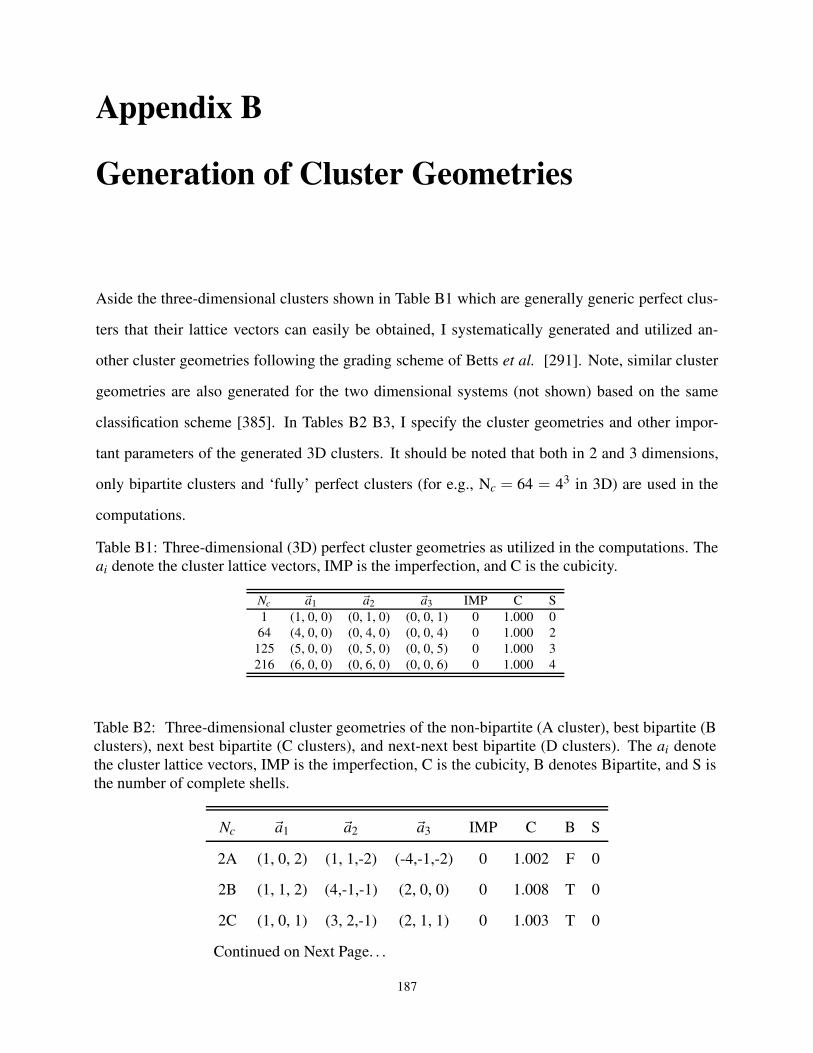
Appendix B
Generation of Cluster Geometries
Aside the three-dimensional clusters shown in Table B1 which are generally generic perfect clus-
ters that their lattice vectors can easily be obtained, I systematically generated and utilized an-
other cluster geometries following the grading scheme of Betts et al. [291]. Note, similar cluster
geometries are also generated for the two dimensional systems (not shown) based on the same
classification scheme [385]. In Tables B2 B3, I specify the cluster geometries and other impor-
tant parameters of the generated 3D clusters. It should be noted that both in 2 and 3 dimensions,
only bipartite clusters and ‘fully’ perfect clusters (for e.g., Nc = 64 = 43 in 3D) are used in the
computations.
Table B1: Three-dimensional (3D) perfect cluster geometries as utilized in the computations. The
ai denote the cluster lattice vectors, IMP is the imperfection, and C is the cubicity.
Nc ~a1 ~a2 ~a3 IMP C S
1 (1, 0, 0) (0, 1, 0) (0, 0, 1) 0 1.000 0
64 (4, 0, 0) (0, 4, 0) (0, 0, 4) 0 1.000 2
125 (5, 0, 0) (0, 5, 0) (0, 0, 5) 0 1.000 3
216 (6, 0, 0) (0, 6, 0) (0, 0, 6) 0 1.000 4
Table B2: Three-dimensional cluster geometries of the non-bipartite (A cluster), best bipartite (B
clusters), next best bipartite (C clusters), and next-next best bipartite (D clusters). The ai denote
the cluster lattice vectors, IMP is the imperfection, C is the cubicity, B denotes Bipartite, and S is
the number of complete shells.
Nc ~a1 ~a2 ~a3 IMP C B S
2A (1, 0, 2) (1, 1,-2) (-4,-1,-2) 0 1.002 F 0
2B (1, 1, 2) (4,-1,-1) (2, 0, 0) 0 1.008 T 0
2C (1, 0, 1) (3, 2,-1) (2, 1, 1) 0 1.003 T 0
Continued on Next Page. . .
187
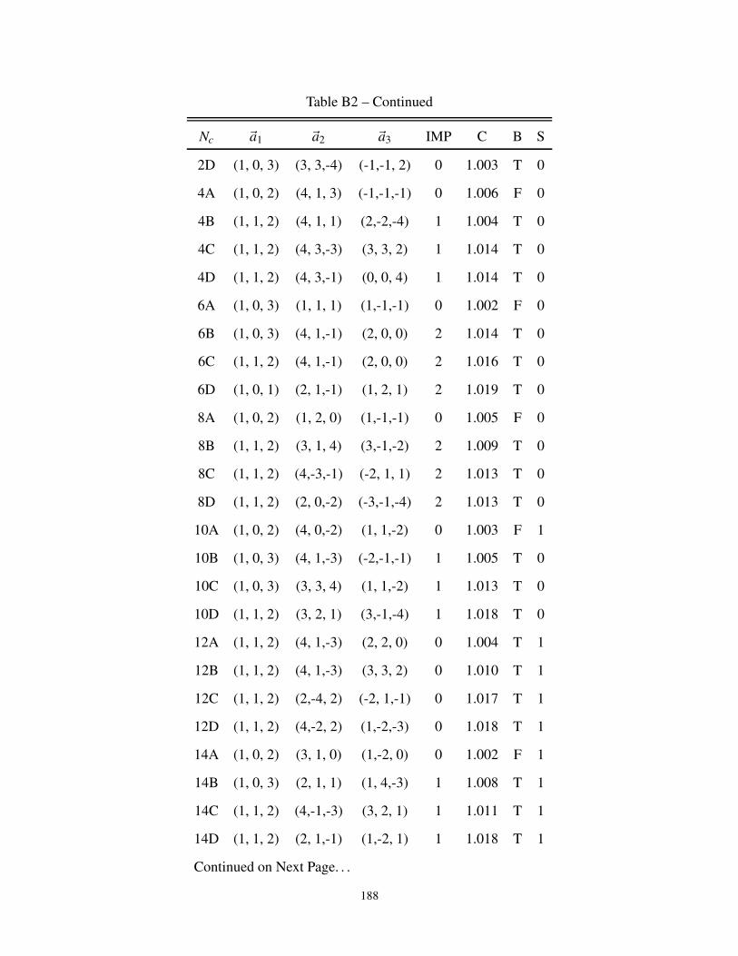
Table B2 – Continued
Nc ~a1 ~a2 ~a3 IMP C B S
2D (1, 0, 3) (3, 3,-4) (-1,-1, 2) 0 1.003 T 0
4A (1, 0, 2) (4, 1, 3) (-1,-1,-1) 0 1.006 F 0
4B (1, 1, 2) (4, 1, 1) (2,-2,-4) 1 1.004 T 0
4C (1, 1, 2) (4, 3,-3) (3, 3, 2) 1 1.014 T 0
4D (1, 1, 2) (4, 3,-1) (0, 0, 4) 1 1.014 T 0
6A (1, 0, 3) (1, 1, 1) (1,-1,-1) 0 1.002 F 0
6B (1, 0, 3) (4, 1,-1) (2, 0, 0) 2 1.014 T 0
6C (1, 1, 2) (4, 1,-1) (2, 0, 0) 2 1.016 T 0
6D (1, 0, 1) (2, 1,-1) (1, 2, 1) 2 1.019 T 0
8A (1, 0, 2) (1, 2, 0) (1,-1,-1) 0 1.005 F 0
8B (1, 1, 2) (3, 1, 4) (3,-1,-2) 2 1.009 T 0
8C (1, 1, 2) (4,-3,-1) (-2, 1, 1) 2 1.013 T 0
8D (1, 1, 2) (2, 0,-2) (-3,-1,-4) 2 1.013 T 0
10A (1, 0, 2) (4, 0,-2) (1, 1,-2) 0 1.003 F 1
10B (1, 0, 3) (4, 1,-3) (-2,-1,-1) 1 1.005 T 0
10C (1, 0, 3) (3, 3, 4) (1, 1,-2) 1 1.013 T 0
10D (1, 1, 2) (3, 2, 1) (3,-1,-4) 1 1.018 T 0
12A (1, 1, 2) (4, 1,-3) (2, 2, 0) 0 1.004 T 1
12B (1, 1, 2) (4, 1,-3) (3, 3, 2) 0 1.010 T 1
12C (1, 1, 2) (2,-4, 2) (-2, 1,-1) 0 1.017 T 1
12D (1, 1, 2) (4,-2, 2) (1,-2,-3) 0 1.018 T 1
14A (1, 0, 2) (3, 1, 0) (1,-2, 0) 0 1.002 F 1
14B (1, 0, 3) (2, 1, 1) (1, 4,-3) 1 1.008 T 1
14C (1, 1, 2) (4,-1,-3) (3, 2, 1) 1 1.011 T 1
14D (1, 1, 2) (2, 1,-1) (1,-2, 1) 1 1.018 T 1
Continued on Next Page. . .
188
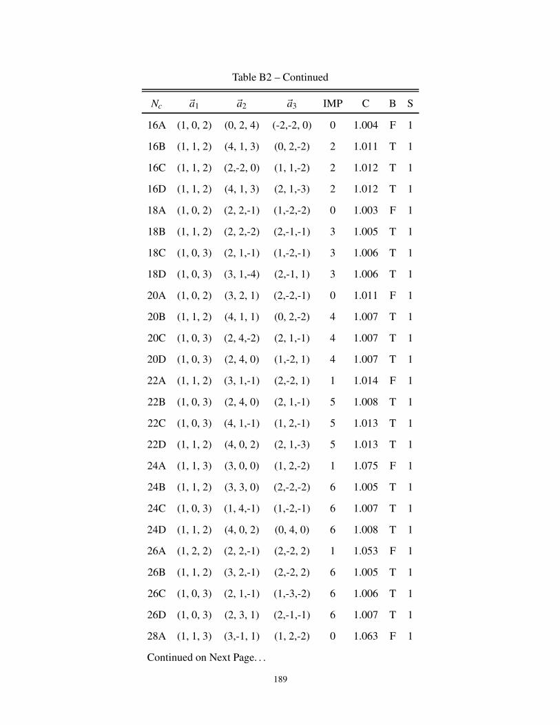
Table B2 – Continued
Nc ~a1 ~a2 ~a3 IMP C B S
16A (1, 0, 2) (0, 2, 4) (-2,-2, 0) 0 1.004 F 1
16B (1, 1, 2) (4, 1, 3) (0, 2,-2) 2 1.011 T 1
16C (1, 1, 2) (2,-2, 0) (1, 1,-2) 2 1.012 T 1
16D (1, 1, 2) (4, 1, 3) (2, 1,-3) 2 1.012 T 1
18A (1, 0, 2) (2, 2,-1) (1,-2,-2) 0 1.003 F 1
18B (1, 1, 2) (2, 2,-2) (2,-1,-1) 3 1.005 T 1
18C (1, 0, 3) (2, 1,-1) (1,-2,-1) 3 1.006 T 1
18D (1, 0, 3) (3, 1,-4) (2,-1, 1) 3 1.006 T 1
20A (1, 0, 2) (3, 2, 1) (2,-2,-1) 0 1.011 F 1
20B (1, 1, 2) (4, 1, 1) (0, 2,-2) 4 1.007 T 1
20C (1, 0, 3) (2, 4,-2) (2, 1,-1) 4 1.007 T 1
20D (1, 0, 3) (2, 4, 0) (1,-2, 1) 4 1.007 T 1
22A (1, 1, 2) (3, 1,-1) (2,-2, 1) 1 1.014 F 1
22B (1, 0, 3) (2, 4, 0) (2, 1,-1) 5 1.008 T 1
22C (1, 0, 3) (4, 1,-1) (1, 2,-1) 5 1.013 T 1
22D (1, 1, 2) (4, 0, 2) (2, 1,-3) 5 1.013 T 1
24A (1, 1, 3) (3, 0, 0) (1, 2,-2) 1 1.075 F 1
24B (1, 1, 2) (3, 3, 0) (2,-2,-2) 6 1.005 T 1
24C (1, 0, 3) (1, 4,-1) (1,-2,-1) 6 1.007 T 1
24D (1, 1, 2) (4, 0, 2) (0, 4, 0) 6 1.008 T 1
26A (1, 2, 2) (2, 2,-1) (2,-2, 2) 1 1.053 F 1
26B (1, 1, 2) (3, 2,-1) (2,-2, 2) 6 1.005 T 1
26C (1, 0, 3) (2, 1,-1) (1,-3,-2) 6 1.006 T 1
26D (1, 0, 3) (2, 3, 1) (2,-1,-1) 6 1.007 T 1
28A (1, 1, 3) (3,-1, 1) (1, 2,-2) 0 1.063 F 1
Continued on Next Page. . .
189
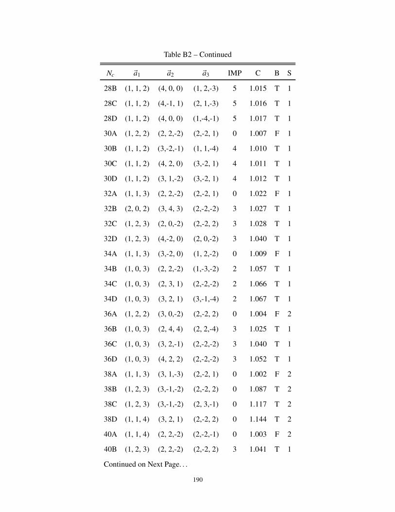
Table B2 – Continued
Nc ~a1 ~a2 ~a3 IMP C B S
28B (1, 1, 2) (4, 0, 0) (1, 2,-3) 5 1.015 T 1
28C (1, 1, 2) (4,-1, 1) (2, 1,-3) 5 1.016 T 1
28D (1, 1, 2) (4, 0, 0) (1,-4,-1) 5 1.017 T 1
30A (1, 2, 2) (2, 2,-2) (2,-2, 1) 0 1.007 F 1
30B (1, 1, 2) (3,-2,-1) (1, 1,-4) 4 1.010 T 1
30C (1, 1, 2) (4, 2, 0) (3,-2, 1) 4 1.011 T 1
30D (1, 1, 2) (3, 1,-2) (3,-2, 1) 4 1.012 T 1
32A (1, 1, 3) (2, 2,-2) (2,-2, 1) 0 1.022 F 1
32B (2, 0, 2) (3, 4, 3) (2,-2,-2) 3 1.027 T 1
32C (1, 2, 3) (2, 0,-2) (2,-2, 2) 3 1.028 T 1
32D (1, 2, 3) (4,-2, 0) (2, 0,-2) 3 1.040 T 1
34A (1, 1, 3) (3,-2, 0) (1, 2,-2) 0 1.009 F 1
34B (1, 0, 3) (2, 2,-2) (1,-3,-2) 2 1.057 T 1
34C (1, 0, 3) (2, 3, 1) (2,-2,-2) 2 1.066 T 1
34D (1, 0, 3) (3, 2, 1) (3,-1,-4) 2 1.067 T 1
36A (1, 2, 2) (3, 0,-2) (2,-2, 2) 0 1.004 F 2
36B (1, 0, 3) (2, 4, 4) (2, 2,-4) 3 1.025 T 1
36C (1, 0, 3) (3, 2,-1) (2,-2,-2) 3 1.040 T 1
36D (1, 0, 3) (4, 2, 2) (2,-2,-2) 3 1.052 T 1
38A (1, 1, 3) (3, 1,-3) (2,-2, 1) 0 1.002 F 2
38B (1, 2, 3) (3,-1,-2) (2,-2, 2) 0 1.087 T 2
38C (1, 2, 3) (3,-1,-2) (2, 3,-1) 0 1.117 T 2
38D (1, 1, 4) (3, 2, 1) (2,-2, 2) 0 1.144 T 2
40A (1, 1, 4) (2, 2,-2) (2,-2,-1) 0 1.003 F 2
40B (1, 2, 3) (2, 2,-2) (2,-2, 2) 3 1.041 T 1
Continued on Next Page. . .
190
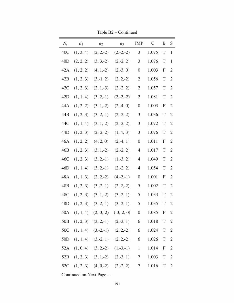
Table B2 – Continued
Nc ~a1 ~a2 ~a3 IMP C B S
40C (1, 3, 4) (2, 2,-2) (2,-2,-2) 3 1.075 T 1
40D (2, 2, 2) (3, 3,-2) (2,-2, 2) 3 1.076 T 1
42A (1, 2, 2) (4, 1,-2) (2,-3, 0) 0 1.003 F 2
42B (1, 2, 3) (3,-1, 2) (2, 2,-2) 2 1.056 T 2
42C (1, 2, 3) (2, 1,-3) (2,-2, 2) 2 1.057 T 2
42D (1, 1, 4) (3, 2,-1) (2,-2,-2) 2 1.081 T 2
44A (1, 2, 2) (3, 1,-2) (2,-4, 0) 0 1.003 F 2
44B (1, 2, 3) (3, 2,-1) (2,-2, 2) 3 1.036 T 2
44C (1, 1, 4) (3, 1,-2) (2,-2, 2) 3 1.072 T 2
44D (1, 2, 3) (2,-2, 2) (1, 4,-3) 3 1.076 T 2
46A (1, 2, 2) (4, 2, 0) (2,-4, 1) 0 1.011 F 2
46B (1, 2, 3) (3, 1,-2) (2,-2, 2) 4 1.017 T 2
46C (1, 2, 3) (3, 2,-1) (1,-3, 2) 4 1.049 T 2
46D (1, 1, 4) (3, 2,-1) (2,-2, 2) 4 1.054 T 2
48A (1, 1, 3) (2, 2,-2) (4,-2,-1) 0 1.001 F 2
48B (1, 2, 3) (3,-2, 1) (2, 2,-2) 5 1.002 T 2
48C (1, 2, 3) (3, 1,-2) (3,-2, 1) 5 1.033 T 2
48D (1, 2, 3) (3, 2,-1) (3,-2, 1) 5 1.035 T 2
50A (1, 1, 4) (2,-3,-2) (-3,-2, 0) 0 1.085 F 2
50B (1, 2, 3) (3, 2,-1) (2,-3, 1) 6 1.018 T 2
50C (1, 1, 4) (3,-2,-1) (2, 2,-2) 6 1.024 T 2
50D (1, 1, 4) (3,-2, 1) (2, 2,-2) 6 1.026 T 2
52A (1, 0, 4) (3, 2,-2) (1,-3,-1) 1 1.014 F 2
52B (1, 2, 3) (3, 1,-2) (2,-3, 1) 7 1.003 T 2
52C (1, 2, 3) (4, 0,-2) (2,-2, 2) 7 1.016 T 2
Continued on Next Page. . .
191

Table B2 – Continued
Nc ~a1 ~a2 ~a3 IMP C B S
52D (1, 2, 3) (2, 2,-2) (2,-4, 0) 7 1.024 T 2
54A (1, 2, 2) (3, 1,-3) (2,-2, 4) 2 1.008 F 2
54B (1, 2, 3) (3,-3, 0) (2, 2,-2) 8 1.004 T 2
54C (1, 2, 3) (3, 3,-2) (2,-2, 2) 8 1.010 T 2
54D (1, 2, 3) (3, 2,-1) (3,-3, 0) 8 1.028 T 2
56A (1, 2, 3) (4, 0,-2) (-3, 2,-2) 2 1.069 F 2
56B (1, 2, 3) (2, 2,-2) (2,-4, 2) 9 1.006 T 2
56C (1, 2, 3) (4,-2, 0) (2, 2,-2) 9 1.007 T 2
56D (1, 2, 3) (3,-4,-3) (2, 2,-2) 9 1.015 T 2
58A (1, 1, 3) (4,-2, 4) (3, 2,-2) 3 1.014 F 2
58B (1, 2, 3) (4, 3,-1) (2,-2, 2) 10 1.004 T 2
58C (1, 2, 3) (3, 1,-4) (2,-2, 2) 10 1.005 T 2
58D (1, 2, 3) (3,-3, 2) (2, 2,-2) 10 1.011 T 2
60A (2, 0, 3) (2, 3,-2) (2,-3,-2) 4 1.001 F 2
60B (1, 1, 4) (4,-2, 0) (2, 2,-2) 11 1.010 T 2
60C (1, 2, 3) (3,-4,-1) (2, 2,-2) 11 1.010 T 2
60D (1, 2, 3) (3,-3, 2) (2, 1,-3) 11 1.011 T 2
62A (1, 2, 4) (3, 0,-2) (2,-3, 2) 5 1.018 F 2
62B (1, 2, 3) (3, 2,-1) (3,-3, 2) 12 1.003 T 2
62C (1, 2, 3) (3,-3, 4) (2, 2,-2) 12 1.022 T 2
62D (1, 2, 3) (4,-3,-1) (2, 2,-2) 12 1.025 T 2
64A (1, 3, 3) (2, 4,-2) (2,-3, 2) 5 1.115 F 1
64B (1, 2, 3) (4, 2,-2) (3,-2, 1) 12 1.002 T 2
64C (1, 2, 3) (3, 4,-1) (3,-2, 1) 12 1.003 T 2
64D (1, 2, 3) (3,-2, 1) (2, 4,-2) 12 1.003 T 2
Continued on Next Page. . .
192

Table B2 – Continued
Nc ~a1 ~a2 ~a3 IMP C B S
66A (1, 2, 4) (3,-2, 2) (2, 1,-4) 4 1.108 F 2
66B (1, 3, 4) (3, 0,-3) (2,-2, 2) 11 1.011 T 2
66C (1, 2, 3) (3, 0,-3) (3,-3, 2) 11 1.026 T 2
66D (1, 1, 4) (3, 2,-3) (2,-3,-1) 11 1.033 T 2
68A (1, 2, 4) (2, 2,-3) (-3, 2,-2) 4 1.051 F 2
68B (1, 3, 4) (2, 2,-2) (2,-4, 0) 11 1.018 T 2
68C (1, 3, 4) (4, 2, 0) (2,-2, 2) 11 1.020 T 2
68D (1, 3, 4) (2, 4,-2) (2,-2, 2) 11 1.022 T 2
70A (1, 2, 4) (3, 1,-3) (3,-2, 2) 1 1.060 F 2
70B (1, 2, 3) (3, 3,-2) (2,-4, 0) 9 1.028 T 2
70C (1, 2, 3) (4, 0,-2) (3,-3, 2) 9 1.030 T 2
70D (1, 2, 3) (3, 3,-2) (3,-2, 3) 9 1.034 T 2
72A (1, 3, 3) (3, 2,-2) (3,-2, 2) 1 1.010 F 2
72B (1, 2, 3) (3,-3, 2) (2, 4,-2) 8 1.047 T 2
72C (1, 2, 3) (4,-2,-2) (3, 4,-1) 8 1.050 T 2
72D (1, 2, 3) (4,-1,-3) (3,-3, 2) 8 1.050 T 2
74A (1, 3, 3) (3, 2,-2) (2,-2, 4) 0 1.057 F 3
74B (1, 3, 4) (4,-1,-3) (2,-2, 2) 7 1.021 T 2
74C (1, 2, 3) (3,-3, 2) (2, 3,-3) 9 1.027 T 2
74D (1, 2, 3) (4,-2,-4) (-3, 3,-2) 10 1.047 T 2
76A (1, 3, 3) (3, 2,-2) (3,-3, 1) 0 1.010 F 3
76B (1, 2, 3) (3, 4,-1) (3,-3, 2) 6 1.026 T 2
76C (1, 2, 3) (3,-3, 2) (2, 2,-4) 6 1.027 T 2
76D (1, 1, 4) (4,-2, 2) (3, 2,-3) 6 1.080 T 2
78A (1, 2, 4) (3,-2, 2) (2, 3,-3) 0 1.043 F 3
Continued on Next Page. . .
193
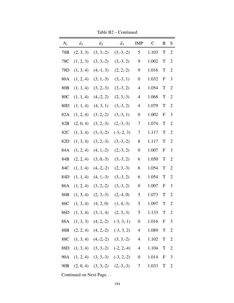
Table B2 – Continued
Nc ~a1 ~a2 ~a3 IMP C B S
78B (2, 3, 3) (3, 3,-2) (3,-3,-2) 5 1.103 T 2
78C (1, 2, 3) (3, 3,-2) (3,-3, 2) 9 1.002 T 2
78D (1, 3, 4) (4,-1, 3) (2, 2,-2) 9 1.016 T 2
80A (1, 2, 4) (3, 1,-3) (3,-3, 1) 0 1.032 F 3
80B (1, 1, 4) (3, 2,-3) (3,-3, 2) 4 1.054 T 2
80C (1, 1, 4) (4,-2, 2) (2, 3,-3) 4 1.068 T 2
80D (1, 1, 4) (4, 3, 1) (3,-3, 2) 4 1.079 T 2
82A (1, 2, 4) (3, 2,-2) (3,-3, 1) 0 1.002 F 3
82B (2, 0, 4) (3, 2,-3) (2,-3,-3) 7 1.074 T 2
82C (1, 3, 4) (3,-3,-2) (-3,-2, 3) 7 1.117 T 2
82D (1, 3, 4) (3, 2,-3) (3,-3,-2) 8 1.117 T 2
84A (1, 2, 4) (4, 1,-2) (2,-3, 2) 0 1.007 F 3
84B (2, 2, 4) (3, 0,-3) (3,-3, 2) 6 1.050 T 2
84C (1, 1, 4) (4,-2,-2) (2, 3,-3) 6 1.054 T 2
84D (1, 1, 4) (4, 1,-3) (3,-3, 2) 6 1.054 T 2
86A (1, 2, 4) (3, 2,-2) (3,-3, 2) 0 1.007 F 3
86B (1, 3, 4) (2, 3,-3) (2,-4, 0) 5 1.073 T 2
86C (1, 3, 4) (4, 2, 0) (1, 4,-3) 5 1.097 T 2
86D (1, 3, 4) (3,-1, 4) (2, 3,-3) 5 1.133 T 2
88A (1, 3, 3) (4, 2,-2) (-3, 3,-1) 0 1.016 F 3
88B (2, 2, 4) (4, 2,-2) (-3, 3, 2) 4 1.089 T 2
88C (1, 3, 4) (4,-2,-2) (3, 3,-2) 4 1.102 T 2
88D (1, 3, 4) (3, 3,-2) (-2, 2,-4) 4 1.104 T 2
90A (1, 2, 4) (3, 3,-3) (-3, 2,-2) 0 1.014 F 3
90B (2, 0, 4) (3, 3,-2) (2,-3,-3) 7 1.033 T 2
Continued on Next Page. . .
194
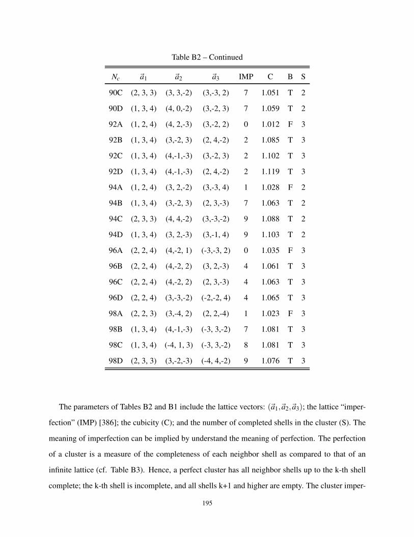
Table B2 – Continued
Nc ~a1 ~a2 ~a3 IMP C B S
90C (2, 3, 3) (3, 3,-2) (3,-3, 2) 7 1.051 T 2
90D (1, 3, 4) (4, 0,-2) (3,-2, 3) 7 1.059 T 2
92A (1, 2, 4) (4, 2,-3) (3,-2, 2) 0 1.012 F 3
92B (1, 3, 4) (3,-2, 3) (2, 4,-2) 2 1.085 T 3
92C (1, 3, 4) (4,-1,-3) (3,-2, 3) 2 1.102 T 3
92D (1, 3, 4) (4,-1,-3) (2, 4,-2) 2 1.119 T 3
94A (1, 2, 4) (3, 2,-2) (3,-3, 4) 1 1.028 F 2
94B (1, 3, 4) (3,-2, 3) (2, 3,-3) 7 1.063 T 2
94C (2, 3, 3) (4, 4,-2) (3,-3,-2) 9 1.088 T 2
94D (1, 3, 4) (3, 2,-3) (3,-1, 4) 9 1.103 T 2
96A (2, 2, 4) (4,-2, 1) (-3,-3, 2) 0 1.035 F 3
96B (2, 2, 4) (4,-2, 2) (3, 2,-3) 4 1.061 T 3
96C (2, 2, 4) (4,-2, 2) (2, 3,-3) 4 1.063 T 3
96D (2, 2, 4) (3,-3,-2) (-2,-2, 4) 4 1.065 T 3
98A (2, 2, 3) (3,-4, 2) (2, 2,-4) 1 1.023 F 3
98B (1, 3, 4) (4,-1,-3) (-3, 3,-2) 7 1.081 T 3
98C (1, 3, 4) (-4, 1, 3) (-3, 3,-2) 8 1.081 T 3
98D (2, 3, 3) (3,-2,-3) (-4, 4,-2) 9 1.076 T 3
The parameters of Tables B2 and B1 include the lattice vectors: (~a1,~a2,~a3); the lattice “imper-
fection” (IMP) [386]; the cubicity (C); and the number of completed shells in the cluster (S). The
meaning of imperfection can be implied by understand the meaning of perfection. The perfection
of a cluster is a measure of the completeness of each neighbor shell as compared to that of an
infinite lattice (cf. Table B3). Hence, a perfect cluster has all neighbor shells up to the k-th shell
complete; the k-th shell is incomplete, and all shells k+1 and higher are empty. The cluster imper-
195
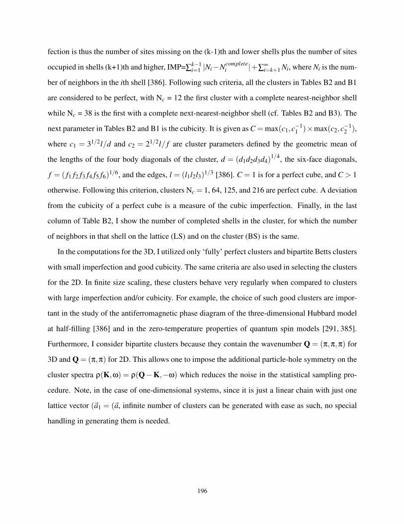
fection is thus the number of sites missing on the (k-1)th and lower shells plus the number of sites
occupied in shells (k+1)th and higher, IMP=∑k−1i=1 |Ni−N
completei |+∑∞
i=k+1 Ni, where Ni is the num-
ber of neighbors in the ith shell [386]. Following such criteria, all the clusters in Tables B2 and B1
are considered to be perfect, with Nc = 12 the first cluster with a complete nearest-neighbor shell
while Nc = 38 is the first with a complete next-nearest-neighbor shell (cf. Tables B2 and B3). The
next parameter in Tables B2 and B1 is the cubicity. It is given as C = max(c1,c−11 )×max(c2,c
−12 ),
where c1 = 31/2l/d and c2 = 21/2l/ f are cluster parameters defined by the geometric mean of
the lengths of the four body diagonals of the cluster, d = (d1d2d3d4)1/4
, the six-face diagonals,
f = ( f1 f2 f3 f4 f5 f6)1/6, and the edges, l = (l1l2l3)
1/3 [386]. C = 1 is for a perfect cube, and C > 1
otherwise. Following this criterion, clusters Nc = 1, 64, 125, and 216 are perfect cube. A deviation
from the cubicity of a perfect cube is a measure of the cubic imperfection. Finally, in the last
column of Table B2, I show the number of completed shells in the cluster, for which the number
of neighbors in that shell on the lattice (LS) and on the cluster (BS) is the same.
In the computations for the 3D, I utilized only ‘fully’ perfect clusters and bipartite Betts clusters
with small imperfection and good cubicity. The same criteria are also used in selecting the clusters
for the 2D. In finite size scaling, these clusters behave very regularly when compared to clusters
with large imperfection and/or cubicity. For example, the choice of such good clusters are impor-
tant in the study of the antiferromagnetic phase diagram of the three-dimensional Hubbard model
at half-filling [386] and in the zero-temperature properties of quantum spin models [291, 385].
Furthermore, I consider bipartite clusters because they contain the wavenumber Q = (π,π,π) for
3D and Q = (π,π) for 2D. This allows one to impose the additional particle-hole symmetry on the
cluster spectra ρ(K,ω) = ρ(Q−K,−ω) which reduces the noise in the statistical sampling pro-
cedure. Note, in the case of one-dimensional systems, since it is just a linear chain with just one
lattice vector (~a1 = (~a, infinite number of clusters can be generated with ease as such, no special
handling in generating them is needed.
196

Table B3: Explicit description of the neighbors sites in three-dimensional clusters showing the
shell number (with the nearest neighbor shell being 1, etc.), number of neighbors in that shell
on the lattice (LS), and the number of neighbors in that shell on the cluster (BS) for the various
clusters in Table B2. The smaller clusters with a full nearest-neighbor shell (Sh) have Nc = 12, the
smaller clusters with a complete next-nearest-neighbor shell have Nc = 38, and with a complete
next-next-nearest-neighbor shell have Nc = 92.
Nc Sh LS BS Nc Sh LS BS Nc Sh LS BS Nc Sh LS BS
2A 1 6 1 2B 1 6 1 2C 1 6 1 2D 1 6 1
4A 1 6 3 4B 1 6 2 4C 1 6 2 4D 1 6 2
– – – 2 18 1 2 18 1 2 18 1
6A 1 6 5 6B 1 6 3 6C 1 6 3 6D 1 6 3
– – – 2 18 2 2 18 2 2 18 2
8A 1 6 6 8B 1 6 4 8C 1 6 4 8D 1 6 4
2 18 1 2 18 3 2 18 3 2 18 3
10A 1 6 6 10B 1 6 5 10C 1 6 5 10D 1 6 5
2 18 3 2 18 4 2 18 4 2 18 4
12A 1 6 6 12B 1 6 6 12C 1 6 6 12D 1 6 6
2 18 5 2 18 5 2 18 5 2 18 5
14A 1 6 6 14B 1 6 6 14C 1 6 6 14D 1 6 6
2 18 7 2 18 6 2 18 6 2 18 6
– – – 3 38 1 3 38 1 3 38 1
16A 1 6 6 16B 1 6 6 16C 1 6 6 16D 1 6 6
2 18 9 2 18 7 2 18 7 2 18 7
– – – 3 38 2 3 38 2 3 38 2
18A 1 6 6 18B 1 6 6 18C 1 6 6 18D 1 6 6
2 18 11 2 18 8 2 18 3 2 18 3
– – – 3 38 3 3 38 3 3 38 3
20A 1 6 6 20B 1 6 6 20C 1 6 6 20D 1 6 6
Continued on Next Page. . .
197
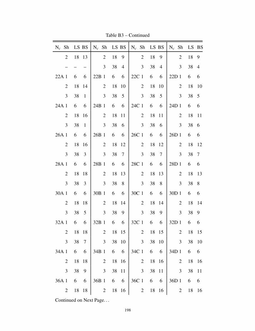
Table B3 – Continued
Nc Sh LS BS Nc Sh LS BS Nc Sh LS BS Nc Sh LS BS
2 18 13 2 18 9 2 18 9 2 18 9
– – – 3 38 4 3 38 4 3 38 4
22A 1 6 6 22B 1 6 6 22C 1 6 6 22D 1 6 6
2 18 14 2 18 10 2 18 10 2 18 10
3 38 1 3 38 5 3 38 5 3 38 5
24A 1 6 6 24B 1 6 6 24C 1 6 6 24D 1 6 6
2 18 16 2 18 11 2 18 11 2 18 11
3 38 1 3 38 6 3 38 6 3 38 6
26A 1 6 6 26B 1 6 6 26C 1 6 6 26D 1 6 6
2 18 16 2 18 12 2 18 12 2 18 12
3 38 3 3 38 7 3 38 7 3 38 7
28A 1 6 6 28B 1 6 6 28C 1 6 6 28D 1 6 6
2 18 18 2 18 13 2 18 13 2 18 13
3 38 3 3 38 8 3 38 8 3 38 8
30A 1 6 6 30B 1 6 6 30C 1 6 6 30D 1 6 6
2 18 18 2 18 14 2 18 14 2 18 14
3 38 5 3 38 9 3 38 9 3 38 9
32A 1 6 6 32B 1 6 6 32C 1 6 6 32D 1 6 6
2 18 18 2 18 15 2 18 15 2 18 15
3 38 7 3 38 10 3 38 10 3 38 10
34A 1 6 6 34B 1 6 6 34C 1 6 6 34D 1 6 6
2 18 18 2 18 16 2 18 16 2 18 16
3 38 9 3 38 11 3 38 11 3 38 11
36A 1 6 6 36B 1 6 6 36C 1 6 6 36D 1 6 6
2 18 18 2 18 16 2 18 16 2 18 16
Continued on Next Page. . .
198
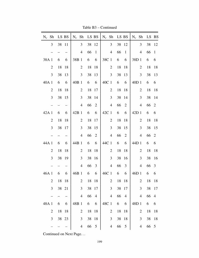
Table B3 – Continued
Nc Sh LS BS Nc Sh LS BS Nc Sh LS BS Nc Sh LS BS
3 38 11 3 38 12 3 38 12 3 38 12
– – – 4 66 1 4 66 1 4 66 1
38A 1 6 6 38B 1 6 6 38C 1 6 6 38D 1 6 6
2 18 18 2 18 18 2 18 18 2 18 18
3 38 13 3 38 13 3 38 13 3 38 13
40A 1 6 6 40B 1 6 6 40C 1 6 6 40D 1 6 6
2 18 18 2 18 17 2 18 18 2 18 18
3 38 15 3 38 14 3 38 14 3 38 14
– – – 4 66 2 4 66 2 4 66 2
42A 1 6 6 42B 1 6 6 42C 1 6 6 42D 1 6 6
2 18 18 2 18 17 2 18 18 2 18 18
3 38 17 3 38 15 3 38 15 3 38 15
– – – 4 66 2 4 66 2 4 66 2
44A 1 6 6 44B 1 6 6 44C 1 6 6 44D 1 6 6
2 18 18 2 18 18 2 18 18 2 18 18
3 38 19 3 38 16 3 38 16 3 38 16
– – – 4 66 3 4 66 3 4 66 3
46A 1 6 6 46B 1 6 6 46C 1 6 6 46D 1 6 6
2 18 18 2 18 18 2 18 18 2 18 18
3 38 21 3 38 17 3 38 17 3 38 17
– – – 4 66 4 4 66 4 4 66 4
48A 1 6 6 48B 1 6 6 48C 1 6 6 48D 1 6 6
2 18 18 2 18 18 2 18 18 2 18 18
3 38 23 3 38 18 3 38 18 3 38 18
– – – 4 66 5 4 66 5 4 66 5
Continued on Next Page. . .
199
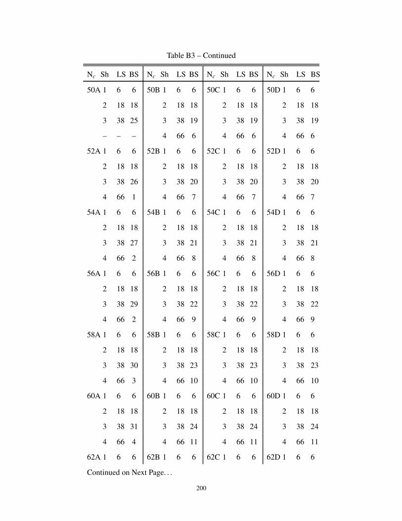
Table B3 – Continued
Nc Sh LS BS Nc Sh LS BS Nc Sh LS BS Nc Sh LS BS
50A 1 6 6 50B 1 6 6 50C 1 6 6 50D 1 6 6
2 18 18 2 18 18 2 18 18 2 18 18
3 38 25 3 38 19 3 38 19 3 38 19
– – – 4 66 6 4 66 6 4 66 6
52A 1 6 6 52B 1 6 6 52C 1 6 6 52D 1 6 6
2 18 18 2 18 18 2 18 18 2 18 18
3 38 26 3 38 20 3 38 20 3 38 20
4 66 1 4 66 7 4 66 7 4 66 7
54A 1 6 6 54B 1 6 6 54C 1 6 6 54D 1 6 6
2 18 18 2 18 18 2 18 18 2 18 18
3 38 27 3 38 21 3 38 21 3 38 21
4 66 2 4 66 8 4 66 8 4 66 8
56A 1 6 6 56B 1 6 6 56C 1 6 6 56D 1 6 6
2 18 18 2 18 18 2 18 18 2 18 18
3 38 29 3 38 22 3 38 22 3 38 22
4 66 2 4 66 9 4 66 9 4 66 9
58A 1 6 6 58B 1 6 6 58C 1 6 6 58D 1 6 6
2 18 18 2 18 18 2 18 18 2 18 18
3 38 30 3 38 23 3 38 23 3 38 23
4 66 3 4 66 10 4 66 10 4 66 10
60A 1 6 6 60B 1 6 6 60C 1 6 6 60D 1 6 6
2 18 18 2 18 18 2 18 18 2 18 18
3 38 31 3 38 24 3 38 24 3 38 24
4 66 4 4 66 11 4 66 11 4 66 11
62A 1 6 6 62B 1 6 6 62C 1 6 6 62D 1 6 6
Continued on Next Page. . .
200
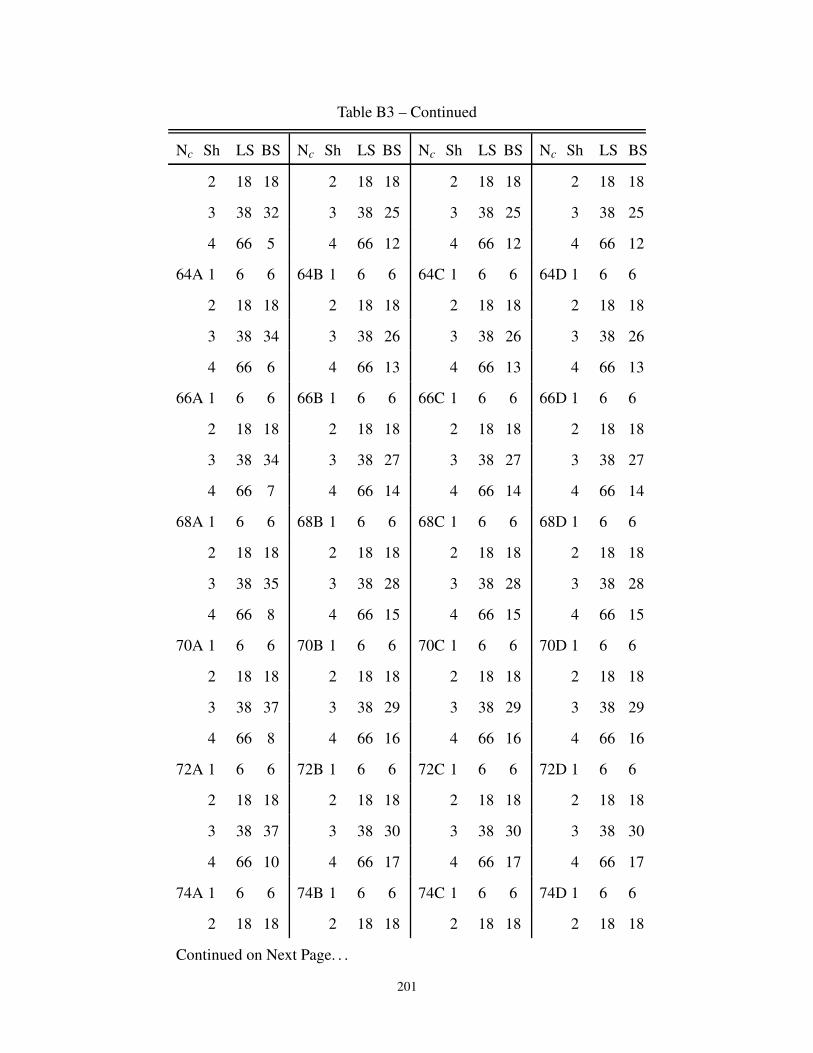
Table B3 – Continued
Nc Sh LS BS Nc Sh LS BS Nc Sh LS BS Nc Sh LS BS
2 18 18 2 18 18 2 18 18 2 18 18
3 38 32 3 38 25 3 38 25 3 38 25
4 66 5 4 66 12 4 66 12 4 66 12
64A 1 6 6 64B 1 6 6 64C 1 6 6 64D 1 6 6
2 18 18 2 18 18 2 18 18 2 18 18
3 38 34 3 38 26 3 38 26 3 38 26
4 66 6 4 66 13 4 66 13 4 66 13
66A 1 6 6 66B 1 6 6 66C 1 6 6 66D 1 6 6
2 18 18 2 18 18 2 18 18 2 18 18
3 38 34 3 38 27 3 38 27 3 38 27
4 66 7 4 66 14 4 66 14 4 66 14
68A 1 6 6 68B 1 6 6 68C 1 6 6 68D 1 6 6
2 18 18 2 18 18 2 18 18 2 18 18
3 38 35 3 38 28 3 38 28 3 38 28
4 66 8 4 66 15 4 66 15 4 66 15
70A 1 6 6 70B 1 6 6 70C 1 6 6 70D 1 6 6
2 18 18 2 18 18 2 18 18 2 18 18
3 38 37 3 38 29 3 38 29 3 38 29
4 66 8 4 66 16 4 66 16 4 66 16
72A 1 6 6 72B 1 6 6 72C 1 6 6 72D 1 6 6
2 18 18 2 18 18 2 18 18 2 18 18
3 38 37 3 38 30 3 38 30 3 38 30
4 66 10 4 66 17 4 66 17 4 66 17
74A 1 6 6 74B 1 6 6 74C 1 6 6 74D 1 6 6
2 18 18 2 18 18 2 18 18 2 18 18
Continued on Next Page. . .
201

Table B3 – Continued
Nc Sh LS BS Nc Sh LS BS Nc Sh LS BS Nc Sh LS BS
3 38 38 3 38 31 3 38 31 3 38 31
4 66 11 4 66 18 4 66 18 4 66 18
76A 1 6 6 76B 1 6 6 76C 1 6 6 76D 1 6 6
2 18 18 2 18 18 2 18 18 2 18 18
3 38 38 3 38 32 3 38 32 3 38 32
4 66 13 4 66 19 4 66 19 4 66 19
78A 1 6 6 78B 1 6 6 78C 1 6 6 78D 1 6 6
2 18 18 2 18 18 2 18 18 2 18 18
3 38 38 3 38 33 3 38 33 3 38 33
4 66 15 4 66 20 4 66 20 4 66 20
– – – – – – 5 102 2 5 102 2
80A 1 6 6 80B 1 6 6 80C 1 6 6 80D 1 6 6
2 18 18 2 18 18 2 18 18 2 18 18
3 38 38 3 38 34 3 38 34 3 38 34
4 66 17 4 66 21 4 66 21 4 66 21
82A 1 6 6 82B 1 6 6 82C 1 6 6 82D 1 6 6
2 18 18 2 18 18 2 18 18 2 18 18
3 38 38 3 38 33 3 38 33 3 38 33
4 66 19 4 66 22 4 66 22 4 66 21
– – – 5 102 2 5 102 2 5 102 2
– – – – – – – – – 6 146 6
84A 1 6 6 84B 1 6 6 84C 1 6 6 84D 1 6 6
2 18 18 2 18 18 2 18 18 2 18 18
3 38 38 3 38 34 3 38 34 3 38 34
4 66 21 4 66 23 4 66 23 4 66 23
Continued on Next Page. . .
202

Table B3 – Continued
Nc Sh LS BS Nc Sh LS BS Nc Sh LS BS Nc Sh LS BS
– – – 5 102 2 5 102 2 5 102 2
86A 1 6 6 86B 1 6 6 86C 1 6 6 86D 1 6 6
2 18 18 2 18 18 2 18 18 2 18 18
3 38 38 3 38 35 3 38 35 3 38 35
4 66 23 4 66 24 4 66 24 4 66 24
– – – 5 102 2 5 102 2 5 102 2
88A 1 6 6 88B 1 6 6 88C 1 6 6 88D 1 6 6
2 18 18 2 18 18 2 18 18 2 18 18
3 38 38 3 38 36 3 38 36 3 38 36
4 66 25 4 66 25 4 66 25 4 66 25
– – – 5 102 2 5 102 2 5 102 2
90A 1 6 6 90B 1 6 6 90C 1 6 6 90D 1 6 6
2 18 18 2 18 18 2 18 18 2 18 18
3 38 38 3 38 35 3 38 35 3 38 35
4 66 27 4 66 26 4 66 26 4 66 26
– – – 5 102 4 5 102 4 5 102 4
92A 1 6 6 92B 1 6 6 92C 1 6 6 92D 1 6 6
2 18 18 2 18 18 2 18 18 2 18 18
3 38 38 3 38 38 3 38 38 3 38 38
4 66 29 4 66 27 4 66 27 4 66 27
– – – 5 102 2 5 102 2 5 102 2
94A 1 6 6 94B 1 6 6 94C 1 6 6 94D 1 6 6
2 18 18 2 18 18 2 18 18 2 18 18
3 38 37 3 38 36 3 38 36 3 38 36
4 66 32 4 66 22 4 66 22 4 66 22
Continued on Next Page. . .
203
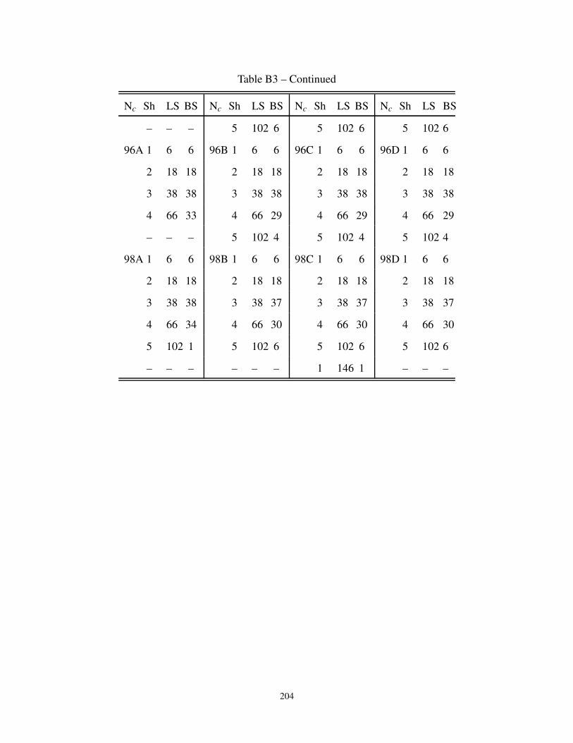
Table B3 – Continued
Nc Sh LS BS Nc Sh LS BS Nc Sh LS BS Nc Sh LS BS
– – – 5 102 6 5 102 6 5 102 6
96A 1 6 6 96B 1 6 6 96C 1 6 6 96D 1 6 6
2 18 18 2 18 18 2 18 18 2 18 18
3 38 38 3 38 38 3 38 38 3 38 38
4 66 33 4 66 29 4 66 29 4 66 29
– – – 5 102 4 5 102 4 5 102 4
98A 1 6 6 98B 1 6 6 98C 1 6 6 98D 1 6 6
2 18 18 2 18 18 2 18 18 2 18 18
3 38 38 3 38 37 3 38 37 3 38 37
4 66 34 4 66 30 4 66 30 4 66 30
5 102 1 5 102 6 5 102 6 5 102 6
– – – – – – 1 146 1 – – –
204

Appendix C
Details of the Transfer Matrix Method
To enable the benchmarking of the TMDCA results, a transfer matrix method was developed. The
transfer matrix method (TMM) [106, 106, 247, 247, 249–251] is an established numerical method
for critical parameters in disordered quantum systems. It is based on a recursive reformulation of
the Schrödinger equation. It has the advantage of capturing the effects of rather a large system sizes
hence, provides quality data for a finite size scaling analysis. In the computations, the transmission
of states through a quasi-1D bar of width M = [6,12] and length L= 2×10⁴M are studied by adding
the products of the transfer matrices with random initial states. A numerical instability arises from
such multiplicative process, which is reduced by orthogonalizing the transfer matrix product in
steps of say five multiplications using a Lapack QR decomposition [132]. The localization edge
is obtained by calculating the dimensionless Kramer-MacKinnon parameter ΛM [250] which is
universal and invariant at the critical point. I.e., ΛM scales as a constant for M →∞ [106]. Thus, we
determine the boundary of the localization transition vis-à-vis the critical disorder strength [223]
by performing a linear fit to ΛM vs. M data. Localized states will have a negative slope and positive
for the extended states. The transfer-matrix method finite size effects are larger for weak disorder
where the states decay slowly with distance and so have large values of ΛM that carry a large
variation in the data. The CPA and DCA are, in fact, exact in this limit as such, do not suffer this
finite size effect.
Any error quoted in the TMM data are from the difference in the measured Wc from finite size
scaling analysis and the crossing of the systems size M from a plot of Λ v.s. W . The finite size
scaling is performed by expanding Λ near the critical point Λ = f (M/ξ)≈Λc+a1|W −Wc|M1/ν+
· · · , and fitting using a least squares procedure. The power of expansion used for instance in
Figure 7.7 was 3.
205
Appendix D
Details of the Kernel Polynomial Method
To further benchmark the TMDCA results, we developed a version of the kernel polynomial
method [243–246]. The kernel polynomial method [243–246] is a numerical technique for expand-
ing the Green function of many-body quantum systems in orthogonal Chebyshev polynomials. In
the kernel polynomial method analysis, instead of diagonalizing the Hamiltonian directly, the DoS
is expanded in term of an infinite series of Chebyshev polynomials. In practice, the truncated se-
ries leads to Gibbs oscillations, which are damped by a modification of the expansion coefficients.
Following previous studies on the Anderson model, the Jackson kernel is used [245].
206
Appendix E
Spectral Representation of the Second
Order Term in the Self-Energy
The second order perturbation theory self-energy is the expansion up to the second order in U
(O[(U/B)2
]) around the Hartree-corrected host propagator. Generally, it is given in the Matsubara
frequency as in Equation 10.9 which we re-write below for clarity as
Σ(SOPT)c [G ] =− lim
iω→ω+
[
U2
N2c β2 ∑
m,p,P,Q
G(K+Q, iωn+ iνm)G(P+Q, iωp+ iνm)G(P, iωp)
]
.
(E.1)
where Q, P, K are cluster momenta and β is the inverse temperature. In the TMDCA formalism,
one cannot use Equation E.1 in its present form since the cluster problem is solved in real space
and more significantly, it is numerically more advantageous to work in the real frequency than in
the Matsubara frequency (because analytic continuation has to be carried out from the imaginary
frequency to the real frequency in order to get real frequency quantities). Note further that analytic
continuation process can miss important features of the observable being studied if not done care-
fully aside its inability to study zero-temperature physics, which coincidentally, is the regime of
interest in the present study. To avoid such analytic continuation, I convert the Matsubara sums to
real frequency integrals using the spectral representation to obtain Equation 10.10. Below, I will
outline the steps to obtaining Equation 10.10.
To reformulate Equation E.1 in the form that is applicable to the cluster solver utilized in this
work, I used spectral representation
G(iω) =
∫dε
ρ(G(ε))
(iω− ε), (E.2)
where ρ(G(ε)) = − 1πℑG(ε), to convert the Matsubara sums to real frequency integrals. Using
207

Equation E.2 in Equation E.1 one obtains
Σ(SOPT )c (iω) =
U2
N2c
∫ 3
∏i=1
(dεiρ(G(ε))
) 1
β2 ∑m,p
1
iω+ iνm− ε1
1
iωp + iνm− ε2
1
iωp − ε3
=U2
N2c
∫ 3
∏i=1
(dεiρ(G(ε))
) 1
β ∑m
1
iω+ iνm− ε1
1
β ∑p
(1
iωp − ε3− 1
iωp + iνm − ε2
)1
iνm − ε2 + ε3
=U2
N2c
∫ 3
∏i=1
(dεiρ(G(ε))
)(nF(ε3)−nF(ε2))
1
β ∑m
1
iνm − (ε1 − iω)
1
iνm − (ε2 − ε3)
=U2
N2c
∫ 3
∏i=1
(dεiρ(G(ε))
) nF(−ε1)nF(ε2)nF(−ε3)+nF(ε1)nF(−ε2)nF(ε3)
iω− ε1 + ε2 − ε3(E.3)
where site labels have been suppressed, ρG = −1/πℑG , and n f = 1/(eβε+1) is the Fermi function.
Using the fact that 1/(x+ i0+) = P (1/x)− iπδ(x) (where ‘P ’ is the principal value of the integral),
we immediately obtain Equation 10.10 as
ρΣ(ω) =U2
N2c
∫dε1dε2ρG (ε1)ρG(ω− ε1 + ε2)ρG(ε2)
×[n f (−ε1)n f (ε2)n f (−ω+ ε1 − ε2)+n f (ε1)n f (−ε2)n f (ω− ε1 + ε2)
](E.4)
The real part of the interacting self-energy follows immediately from Kronigs-Kramer transform
as
ΣSOPTR (ω) =−P
∫ ∞
∞
ρΣ(ω)
ω−ωdω. (E.5)
Combining the real and the imaginary part, the non-local SOPT self-energy is then obtained as
ΣSOPTc (i, j,ω) = ΣSOPT
R (i, j,ω)− iπρΣ(i, j,ω). (E.6)
Equation E.4 is computational expensive especially since we have both spatial and frequency de-
pendence. In fact, assuming it depends only on frequency, it scales as N3 process (N is the size of
the grid points used in the integration). This N3 process can be reduced to N2 process by splitting
the double integral into two one dimensional integral as
ρΣ(ω) =U2
Nc
∫dε1ρG(−ε1) [nF(ε1)χ1(ω+ ε1)+nF(−ε1)χ2(ω+ ε1)] (E.7)
208
with
χ1(ε) =1
Nc
∫dε1ρG(ε+ ε)ρG(ε)nF(ε)nF(−ε− ε) and (E.8a)
χ2(ε) =1
Nc
∫dε1ρG(ε+ ε)ρG(ε)nF(−ε)nF(ε+ ε) (E.8b)
In arriving at Equation E.7, particle-hole symmetry property have not been used as such, the
above formulation is suitable at and away from half-filling. Utilizing the fast-Fourier transfor-
mation [347], the above N2 process is further reduced to scale as N lnN.
209
Vita
Chinedu Ekuma Ekuma was born and raised in the commercial city of Lagos, Nigeria. He com-
pleted his high school at Festac Grammar school, Festac Town, Lagos. Subsequently, he enrolled
at the Ebonyi State University, Nigeria for his Bachelor degree in science where he graduated as
the overall best graduating student with summa cum laude (1st Class Hons) in Industrial Physics
in the 2005/2006 academy year. He went ahead to serve the compulsory one-year national youth
service corps in Delta state, Nigeria. He was then appointed an Assistant lecturer in the Depart-
ment of Physics, University of Port Harcourt, Nigeria and concurrently, he enrolled and obtained
an MSc in the Department of Physics & Astronomy, University of Nigeria, Nigeria. In the fall
of 2009 he arrived at Southern University, Baton Rouge, LA to pursue an MSc in Computational
Physics after he was awarded the prestigious Ebonyi, Nigeria overseas scholarship for being the
best graduating student of the 2005/2006 academic year. After successfully completing his MSc,
he joined the Department of Physics & Astronomy, Lousiana State University, Baton Rouge, LA in
the fall of 2010. He worked on diverse research projects under the supervision of Dr. Mark Jarrell
with Dr. Juana Moreno as a conjunct advisor where he continued working towards his Ph.D.
210