TOWARDS TRACTABLE PARAMETER-FREE STATISTICAL LEARNING

by

Aaron Angelo D’Souza

A Dissertation Presented to theFACULTY OF THE GRADUATE SCHOOL

UNIVERSITY OF SOUTHERN CALIFORNIAIn Partial Fulfillment of theRequirements for the Degree

DOCTOR OF PHILOSOPHY(COMPUTER SCIENCE)

December 2004

Copyright 2004 Aaron Angelo D’Souza

Dedication

This dissertation is dedicated to a woman of strength and beauty, who taught me much

of what makes me the person I am; my grandmother, Benedicta Correia.

ii

Acknowledgements

It has been a privilege to have had Stefan Schaal as my sensei through this journey.

As if finding a mentor who brings out the best in his students wasn’t enough, I’ve been

lucky to have one who has also grown to be a dear friend. He has provided direction and

inspiration, while giving me the freedom to develop my own ideas and style of research.

Under his wing, our little research group has become family, and our lab has become a

home that I am loth to take leave of. I will miss our extended discussions on statistics,

balrogs, and everything in between.

I could not have accomplished this body of work were it not for the wonderful advice

and support from Sethu Vijayakumar, Andrew Moore, Chris Atkeson and Ashish Goel. I

would especially like to thank Shun-ichi Amari and Mitsuo Kawato for the opportunities

to spend very rewarding periods of time at the RIKEN Brain Science Institute and ATR

Laboratories respectively.

I must also thank our (extended) lab: Aude Billard, Rick Cory, Auke Ijspeert, Shrija

Kumari, Michael Mistry, Peyman Mohajerian, Srideep Musuvathy, Jan Peters & Ladan

Shams for becoming family over the last four years. A special mention goes to Jo-Anne

Ting, who has been a great help, and fabulous sounding board for many crazy research

iii

ideas in this last year. Also to Eric Coe, for providing the best mixture of caffeine, jazz,

sarcasm and friendship anyone could ask for.

My parents Afra & Ayres D’Souza and sister Maria have provided me with the op-

portunities, encouragement and love which have allowed me to reach this far. I hope I

have made them proud. My dear fiancee Jayita Bhojwani has been a pillar of strength,

and the rest of my life with her will not be enough to thank her for loving, encouraging,

prodding, scolding, inspiring and tolerating me during the ups and downs of graduate

student life.

iv

Contents

Dedication ii

Acknowledgements iii

List Of Tables viii

List Of Figures ix

Abstract xi

1 Introduction 11.1 Nuisance Parameters in Statistical Learning . . . . . . . . . . . . . . . . . 51.2 Bayesian Model Complexity Estimation . . . . . . . . . . . . . . . . . . . 81.3 Alternatives to the Evidence Framework . . . . . . . . . . . . . . . . . . . 12

1.3.1 Cross-Validation . . . . . . . . . . . . . . . . . . . . . . . . . . . . 121.3.2 Minimum Description Length . . . . . . . . . . . . . . . . . . . . . 131.3.3 Bayesian/Akaike Information Criteria . . . . . . . . . . . . . . . . 151.3.4 Reversible Jump Markov Chain Monte Carlo . . . . . . . . . . . . 181.3.5 Structural Risk Minimization . . . . . . . . . . . . . . . . . . . . . 20

1.4 Dissertation Outline . . . . . . . . . . . . . . . . . . . . . . . . . . . . . . 23

2 The Quest for Analytical Tractability 252.1 Graphical Models . . . . . . . . . . . . . . . . . . . . . . . . . . . . . . . . 25

2.1.1 Graphical Model Conventions in this Dissertation . . . . . . . . . . 282.2 Inference in Graphical Models . . . . . . . . . . . . . . . . . . . . . . . . . 29

2.2.1 Inferring Marginal Distributions . . . . . . . . . . . . . . . . . . . 302.2.1.1 Variable Elimination . . . . . . . . . . . . . . . . . . . . . 312.2.1.2 Junction Trees . . . . . . . . . . . . . . . . . . . . . . . . 342.2.1.3 Monte Carlo Methods . . . . . . . . . . . . . . . . . . . . 37

2.2.2 Parameter Estimation and the EM Algorithm . . . . . . . . . . . . 382.3 The Factorial Variational Approximation . . . . . . . . . . . . . . . . . . 43

2.3.1 An Update Mechanism for Factored Posterior Distributions . . . . 432.3.2 Solution for Partial Factorization . . . . . . . . . . . . . . . . . . . 452.3.3 The Effect of Making Independence Assumptions . . . . . . . . . . 48

v

3 Algorithms for Analytical Tractability 513.1 Mixture Model Cardinality . . . . . . . . . . . . . . . . . . . . . . . . . . 52

3.1.1 Growing Mixture Models . . . . . . . . . . . . . . . . . . . . . . . 553.1.1.1 1 or 2 Models? . . . . . . . . . . . . . . . . . . . . . . . . 55

3.1.2 An Algorithm for Growing Mixture Model Cardinality . . . . . . . 613.1.3 Application to Non-linear Latent Dimensionality Estimation . . . 643.1.4 Mixture Modeling with Dirichlet Process Priors . . . . . . . . . . . 72

3.2 Online Learning with Automatic Forgetting Rates . . . . . . . . . . . . . 773.2.1 Using a Kalman Filter to Track Non-Stationarity . . . . . . . . . . 793.2.2 Bayesian Forgetting Rates Evaluation . . . . . . . . . . . . . . . . 85

3.2.2.1 On Selecting the Window Size “N” . . . . . . . . . . . . 883.3 Bayesian Supersmoothing . . . . . . . . . . . . . . . . . . . . . . . . . . . 90

3.3.1 An EM-Like Learning Algorithm . . . . . . . . . . . . . . . . . . . 943.3.2 Bayesian Supersmoothing Evaluations . . . . . . . . . . . . . . . . 99

4 The Quest for Computational Tractability 1044.1 Computationally Tractable Linear Regression . . . . . . . . . . . . . . . . 106

4.1.1 Dimensionality Reduction for Regression . . . . . . . . . . . . . . . 1074.1.1.1 Principal Component Regression . . . . . . . . . . . . . . 1084.1.1.2 Joint-Space Factor Analysis for Regression . . . . . . . . 1094.1.1.3 Joint-Space Principal Component Regression . . . . . . . 1114.1.1.4 Kernel Dimensionality Reduction for Regression . . . . . 111

4.1.2 Efficient Decomposition Methods for Regression . . . . . . . . . . 1124.1.2.1 Partial Least Squares Regression . . . . . . . . . . . . . . 1124.1.2.2 Backfitting . . . . . . . . . . . . . . . . . . . . . . . . . . 114

4.2 Data Structures for Fast Statistics . . . . . . . . . . . . . . . . . . . . . . 1164.3 A Probabilistic Derivation of Backfitting . . . . . . . . . . . . . . . . . . . 119

4.3.1 An EM Algorithm for Probabilistic Backfitting . . . . . . . . . . . 1224.3.2 Relating Traditional and Probabilistic Backfitting . . . . . . . . . 1244.3.3 Convergence of Probabilistic Backfitting . . . . . . . . . . . . . . . 126

4.4 Bayesian Backfitting . . . . . . . . . . . . . . . . . . . . . . . . . . . . . . 1274.4.1 Regularizing the Regression Vector Length . . . . . . . . . . . . . 1284.4.2 Regularizing the Number of Relevant Inputs . . . . . . . . . . . . 1324.4.3 Alternative Posterior Factorization . . . . . . . . . . . . . . . . . . 1354.4.4 Extension to Classification . . . . . . . . . . . . . . . . . . . . . . 138

4.4.4.1 Bayesian Backfitting for Classification . . . . . . . . . . . 1414.4.5 Efficient Sparse Bayesian Learning and RVMs . . . . . . . . . . . . 142

4.5 Bayesian Backfitting Experiments . . . . . . . . . . . . . . . . . . . . . . . 1464.5.1 Backfitting RVM Evaluation . . . . . . . . . . . . . . . . . . . . . 149

5 Conclusion 1535.1 Summary of Dissertation Contributions . . . . . . . . . . . . . . . . . . . 1535.2 Opportunities for Further Research . . . . . . . . . . . . . . . . . . . . . . 157

Reference List 160

vi

Appendix ASome Useful Results . . . . . . . . . . . . . . . . . . . . . . . . . . . . . . . . . 170A.1 Schur Complements . . . . . . . . . . . . . . . . . . . . . . . . . . . . . . 170A.2 Some Important Expectations . . . . . . . . . . . . . . . . . . . . . . . . . 171

Appendix BDerivations . . . . . . . . . . . . . . . . . . . . . . . . . . . . . . . . . . . . . . 175B.1 Factorial Variational Approximation . . . . . . . . . . . . . . . . . . . . . 175

B.1.1 Solution for Partial Factorization . . . . . . . . . . . . . . . . . . . 176B.2 Variational Approximation for Mixture Models . . . . . . . . . . . . . . . 177B.3 Variational Approximation for Forgetting Rates . . . . . . . . . . . . . . . 179B.4 Derivation of Probabilistic Backfitting . . . . . . . . . . . . . . . . . . . . 181B.5 Variational Approximation for Bayesian Backfitting . . . . . . . . . . . . . 183

B.5.1 Regularizing the Regression Vector Length . . . . . . . . . . . . . 183B.5.2 Alternative Posterior Factorization . . . . . . . . . . . . . . . . . . 185

vii

List Of Tables

4.1 Results on the neuron-muscle data set . . . . . . . . . . . . . . . . . . . . 148

4.2 Relative computation time . . . . . . . . . . . . . . . . . . . . . . . . . . . 151

viii

List Of Figures

1.1 The Sarcos humanoid robot. . . . . . . . . . . . . . . . . . . . . . . . . . . 3

1.2 Fitting a data set with models of 3 different complexities . . . . . . . . . 8

1.3 Justification for the evidence framework . . . . . . . . . . . . . . . . . . . 10

2.1 An example graphical model . . . . . . . . . . . . . . . . . . . . . . . . . . 28

2.2 Constructing an MRF from a DAG . . . . . . . . . . . . . . . . . . . . . . 30

2.3 Successive steps in the variable elimination algorithm . . . . . . . . . . . . 33

2.4 A triangulated Markov network and its junction tree. . . . . . . . . . . . . 34

2.5 Effect of the independence assumption . . . . . . . . . . . . . . . . . . . . 48

3.1 1 or 2 models? . . . . . . . . . . . . . . . . . . . . . . . . . . . . . . . . . 56

3.2 Justification for evidence based splitting . . . . . . . . . . . . . . . . . . . 60

3.3 Growing mixture models for density estimation . . . . . . . . . . . . . . . 62

3.4 Growing mixture models for regression . . . . . . . . . . . . . . . . . . . . 63

3.5 Graphical model for Bayesian factor analysis . . . . . . . . . . . . . . . . 66

3.6 Local dimensionality reduction . . . . . . . . . . . . . . . . . . . . . . . . 67

3.7 The Sarcos SenSuit . . . . . . . . . . . . . . . . . . . . . . . . . . . . . . . 68

3.8 Histogram of latent dimensionality for movement data . . . . . . . . . . . 69

3.9 Sample distributions from a Dirichlet process . . . . . . . . . . . . . . . . 73

ix

3.10 Bayesian density estimation using Dirichlet process priors . . . . . . . . . 76

3.11 Effect of the forgetting rate on process tracking . . . . . . . . . . . . . . . 80

3.12 Graphical model for variational Kalman filtering . . . . . . . . . . . . . . 81

3.13 Estimating a drifting parameter . . . . . . . . . . . . . . . . . . . . . . . . 84

3.14 MSE comparison across 3 algorithms . . . . . . . . . . . . . . . . . . . . . 86

3.15 Evaluation of Bayesian forgetting factors for multidimensional regression . 87

3.16 Effect of increasing window size on the estimation error . . . . . . . . . . 88

3.17 Estimating the influence of past data . . . . . . . . . . . . . . . . . . . . . 89

3.18 Graphical model for Bayesian supersmoothing . . . . . . . . . . . . . . . . 92

3.19 Evaluation of Bayesian supersmoothing . . . . . . . . . . . . . . . . . . . 103

4.1 Graphical model for linear regression. . . . . . . . . . . . . . . . . . . . . 105

4.2 Structuring data in a KD-tree . . . . . . . . . . . . . . . . . . . . . . . . . 117

4.3 Structuring data in a ball-tree . . . . . . . . . . . . . . . . . . . . . . . . . 118

4.4 Introducing hidden variables for probabilistic backfitting. . . . . . . . . . 120

4.5 Bayesian backfitting corresponding to shrinkage methods . . . . . . . . . . 128

4.6 Bayesian backfitting for ARD models. . . . . . . . . . . . . . . . . . . . . 132

4.7 Alternative factorization for Bayesian backfitting . . . . . . . . . . . . . . 135

4.8 Variational approximation to the logistic function . . . . . . . . . . . . . . 138

4.9 Fitting the sinc function using backfitting-RVM. . . . . . . . . . . . . . . 145

4.10 Results of applying Bayesian backfitting to the neuron-muscle data . . . . 147

4.11 nMSE on benchmark regression datasets . . . . . . . . . . . . . . . . . . . 149

4.12 Benchmark dataset classification error rate . . . . . . . . . . . . . . . . . 150

4.13 Number of “relevant” vectors retained . . . . . . . . . . . . . . . . . . . . 151

x

Abstract

The objectivity of statistical analysis hinges on the assumptions made about the form and

complexity of the model used to fit the data. These usually take the guise of “nuisance

parameters” which must be set based on some meta-level knowledge of the problem to

be solved. This dissertation seeks to contribute statistical methods which require as little

meta-level knowledge as possible, and yet are computationally and analytically tractable

enough to operate on real-world datasets.

This goal is partially achieved within the framework of Bayesian statistics, which

allows the specification of prior knowledge, and lets the data correctly constrain model

complexity. However, for all but the simplest of statistical models, a full Bayesian treat-

ment is often analytically and computationally intractable. We therefore explore the

usefulness of approximation techniques; in particular, those stemming from variational

calculus, to gain analytical tractability when performing statistical inference in complex

graphical models.

We provide a novel, analytically closed-form solution to estimating the cardinality of

mixture models, by locally approximating the evidence for splitting existing models, and

thus growing complexity as needed. We contribute a solution to the problem of estimating

forgetting rates for online learning by modeling the non-stationarity of the model as a set

xi

of drifting parameters, thus allowing a variational Kalman smoother to estimate the time

scale of the process drift. We also address the estimation of Bayesian distance metrics

for locally weighted regression — a problem commonly known as supersmoothing — by

probabilistically modeling the kernel weights assigned to the data.

Another contribution of this dissertation is the development of statistical inference

methods which are computationally scalable. We derive a probabilistic version of back-

fitting — a highly robust and scalable class of supervised non-parametric algorithms —

and demonstrate that, among others, the framework of sparse Bayesian learning arises

from this class as a special case.

We conclude that in several difficult statistical learning problems, principled approx-

imation techniques, and careful model construction can create scalable and robust algo-

rithms which eliminate the most difficult model complexity parameters, while retaining

their applicability to large, complex and underconstrained data sets.

xii

Chapter 1

Introduction

Humans and other biological learning “machines” demonstrate an immense amount of

variability in learning strategies, along with an adaptive ability that spans a wide range

of spatio-temporal scales. In this sense, they are truly autonomous learning entities since

they require little outside intervention to configure the adaptive process.

The last several decades of research in the artificial intelligence and in particular,

machine learning, have been working towards this goal of achieving greater autonomy in

complex adaptive systems that can function in the real world with minimal monitoring

and intervention. However, developing a machine learning framework that can display

the same robustness as its biological counterpart, and operate without modification on

the many noisy, large and underconstrained data sets that the real world has to offer has

been an elusive goal. In some sense, we can regard the autonomy of an intelligent system

at two levels:

Task-level autonomy: Autonomy at this level concerns itself with judging the correct

actions to carry out based on the perceived state of an uncertain environment. A

robot (for example) must choose between various actions or behavior modes that

1

achieve goals or maximize expected rewards. Hierarchical plan generation, and

decisions involving role and resource allocation in groups of intelligent entities also

fall under this domain. Research on planning, reinforcement learning and POMDPs

for example, addresses the autonomy required to accomplish these tasks.

Inference-level autonomy: Task-level autonomy relies on basic statistical operations

such as regression, classification, clustering and density estimation to provide the

building blocks of action and reasoning. For example, an autonomous humanoid

robot requires that the statistical models of its inverse dynamics are constructed

before the task of planning movements and trajectories is successful. This is fun-

damentally a regression problem from the representation of a desired movement, to

the actuator commands required to achieve it. Autonomy at the inference level is

concerned with the construction of such models of the observed data. This type of

autonomy is the primary topic of this dissertation.

When discussing inference-level autonomy, it is important to note the distinction

between choosing the correct model, and optimizing its parameters to fit the data. While

there exists an extensive body of literature that deals with the optimization of model

parameters, this process must necessarily rely on the appropriate model being chosen to

begin with. In particular, a crucial aspect of model choice involves the specification of

its complexity or modeling capacity which directly influences its capability to fit either

simple or complex data sets. As we shall see, incorrectly specifying this “parameter” can

lead to a failure to generalize correctly to unseen data. Even though setting the model

complexity correctly is an important part of model construction, for an intelligent system

2

Figure 1.1: The Sarcos humanoid robot.

that functions in the real world and which faces the task of analyzing data that could

arise from processes of varying complexity, having an oracle specify the correct model

complexity at each instance does not result in a great deal of autonomy.

Besides the requirement of autonomy in specifying the model complexity, this deter-

mination must be achievable in an efficient manner, both in the use of data as well as

computation time. As an example, when learning its own inverse dynamics, the Sarcos

humanoid robot shown in figure 1.1 has a mere 2ms to incorporate new data in to the

existing model and generate a motor command for the following timestep. Also, with

training data being available at such high frequencies, and thus very large quantities, it

becomes necessary to efficiently cache useful statistics from the data such that we are

3

not burdened with processing the entire history every time we wish to generate a useful

prediction.

Of the many approaches to machine learning, the field of statistical learning embod-

ies some of the most promising features that we would expect from truly autonomous

learning:

Representation of uncertainty: Learning machines are faced with numerous sources

of ambiguity and uncertainty. Real-world data is frequently corrupted by noise and

outliers due to sensor limitations. Taking into account this stochasticity is vital to

the success of any learning system. Modeling the learning process as probabilistic

inference can implicitly and explicitly represent the uncertainty in both our assump-

tions about the world and the inference results. In effect, modeling uncertainty gives

us knowledge about the “lack of knowledge”, allowing a learning system to focus

on reducing this uncertainty.

Meta-learning: The ability to “learn how to learn” is a key element of producing robust

learning systems that can adapt to varying degrees of problem type and complexity.

For example, while conventional neural network research has taken inspiration from

biology’s computational structure, it has failed in creating a principled description

of self-regulated learning so often found in biological systems. One of the main

strengths of a statistical learning machine is its ability to mathematically quantify

uncertainty in itself. As we shall see, this feature allows us to perform an impor-

tant component of self-adaptation; automatic determination of statistical model

complexity.

4

1.1 Nuisance Parameters in Statistical Learning

At the core of statistical analysis is the model used to fit the observed data. The most

crucial decision facing the analyst is the structure of this model. Model structure en-

capsulates the key assumptions about the process that is believed to have generated the

data, and hence constrains the analysis results such that it is possible to generalize from

them in a meaningful manner. The exact definition of what constitutes “model struc-

ture” varies drastically as one moves between the various research sub-communities in

machine learning, but a common thread seems to suggest that one should interpret struc-

ture as a set of restrictions on the space of possible hypotheses that can explain the data

(Mitchell 1997). Without assumptions to constrain this space, one can do no better than

to memorize the observed data — a solution that is as trivial as it is useless.

The assumptions used to develop a statistical model can be coarsely divided into two

main categories:

1. Assumptions that describe model form.

2. Assumptions that restrict model complexity.

Often, the first category of assumptions are motivated by constraints of efficiency

and representation ability. For example, efficiency constraints may require us to model

a data set using a collection of computationally efficient locally linear models, while the

knowledge that we are modeling periodic data may prompt us to use a basis space of

sine and cosine functions or von Mises distributions1. Kernel methods, which include the

popular support vector machine (SVM) (Scholkopf & Smola 2000), and Gaussian process

regression (Williams & Rasmussen 1996), feature a particularly direct example of choice

5

in model form, since their function analytic view requires the explicit choice of function

class (polynomial, linear, Gaussian etc.) by choosing the corresponding (combination of)

reproducing kernel Hilbert spaces (RKHSs) within which a solution is to be found.

What we will primarily concern ourselves with throughout this dissertation, is the

second category of assumptions: those that determine the model complexity. Complexity

parameters occur in many forms in statistical learning models. The following list is a

small set of examples:

• Number of assumed latent dimensions for dimensionality reduction.

• Number of components in a mixture model.

• Number of relevant inputs or features for supervised learning.

• Spatio-temporal distance metrics for local learning.

• Size of the window of sufficient statistics in online learning.

A common property of all these parameters is that by tuning them, we can create a

spectrum of models, which are able to fit data sets of various complexities. For example,

assuming a small latent dimensionality in principal component analysis (PCA) allows the

model to only fit a set of simple data sets of low dimensionality, while producing large

errors on data sets with high-dimensional structure. The effects of underestimating model

complexity are easy to detect since we observe poor modeling performance on the so-called

training data set. Overestimating model complexity is a far more difficult problem to

1Defined as p(x) = exp(b cos(x−a))2πI0(b)

for x ∈ [0, 2π) where I0(·) is a modified Bessel function of first kind,

the von Mises distribution is a circular analog of the Normal distribution

6

tackle since the model will perform extremely well on the training data, but fail miserably

when generalizing to unseen examples. This phenomenon is well known in statistical

learning literature as the bias-variance tradeoff (Geman et al. 1992). Essentially, an

overly complex model will fit the (inevitable) noise in an observed data set, and successive

re-training from multiple data sets will result in wildly differing estimates (high variance)

of the model parameters.

In many cases, prior knowledge of the data-generating process may help us make

an educated guess about the correct model complexity. For example, knowing sensor

limitations may help us bound the frequency range of a measured signal, thus introducing

smoothness constraints in the model used to analyze it. However, such knowledge is not

always easy to come by, and may be difficult to infer a priori. Picking the correct values for

these complexity parameters is therefore crucial to the outcome of the inference process,

and yet these are the parameters for which we would most like to have the data tell us

their value. It is little wonder that these complexity variables are often termed “nuisance

parameters”.

As the following section will demonstrate, the framework of graphical modeling, in

combination with the application of Bayesian statistics can provide an elegant solution

to the problem of determining model complexity. However, as we will discuss in chapter

2, more often than not, this solution is analytically and computationally too difficult to

apply to most real-world problems.

7

−1.5 −1 −0.5 0 0.5 1 1.5 2−5

0

5

10

15

20

25

30

35

x

y(x)

DataM

1M

2M

3True

LogModel MSE Evidence LOO-CV

M1 44.85 100.25 78.05

M2 15.55 104.38 25.84

M3 7.92 59.91 901.06

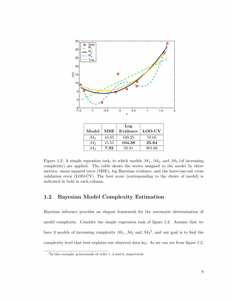
Figure 1.2: A simple regression task, to which models M1, M2, and M3 (of increasingcomplexity) are applied. The table shows the scores assigned to the model by threemetrics: mean squared error (MSE), log Bayesian evidence, and the leave-one-out crossvalidation error (LOO-CV). The best score (corresponding to the choice of model) isindicated in bold in each column.

1.2 Bayesian Model Complexity Estimation

Bayesian inference provides an elegant framework for the automatic determination of

model complexity. Consider the simple regression task of figure 1.2. Assume that we

have 3 models of increasing complexity M1, M2 and M32, and our goal is to find the

complexity level that best explains our observed data xD. As we can see from figure 1.2,

2In this example, polynomials of order 1, 2 and 6, respectively.

8

using a naive goodness-of-fit measure such as mean squared error (MSE) on the training

data, would select the model with the highest complexity since it achieves the least MSE.

The generalization ability (closeness to the true function) however, suffers greatly as the

complexity is over/underestimated.

How can we best determine which of the three models has the correct complexity for

this data set? As a Bayesian inference problem, this is best stated as finding the model

Mi which maximizes:

p(Mi|xD) =p(xD|Mi)p(Mi)

p(xD)(1.1)

If we have no prior preference between the models, then p(M1) = p(M2) = p(M3) =

1/3, and it is the so called evidence p(xD|Mi) that will decide between the models under

consideration. This quantity is fairly polyonymous; statistics literature refers to it as

the “marginal likelihood”, while the physics community calls it the “partition function”.

Notably, this term also features as the normalization constant in the Bayesian inference

of the posterior distribution over unobserved parameters (or hidden variables) xH in a

model, conditioned on the observed variables xD:

p(xH|xD,Mi) =p(xD|xH)p(xH|Mi)

p(xD|Mi)︸ ︷︷ ︸evidence

Does maximizing evidence arrive at the correct choice of model complexity? To answer

this, consider the caricature scenario depicted in figure 1.3 (adapted from (Bishop 1995)).

Each point on the horizontal axis represents a single data set. Low-complexity statistical

9

obse

rved

dat

aset

order 2

(space of all possible N−point datasets)

order 1order 6 xD

p(xD|M)

∫p(

xD|xH

)p(xH|M

)dxH

p(xD|M2)

p(xD|M3)

p(xD|M1)

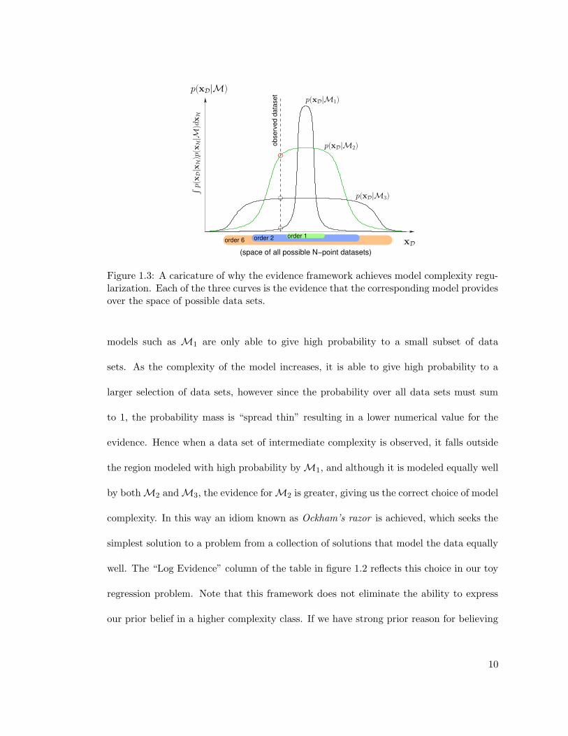
Figure 1.3: A caricature of why the evidence framework achieves model complexity regu-larization. Each of the three curves is the evidence that the corresponding model providesover the space of possible data sets.

models such as M1 are only able to give high probability to a small subset of data

sets. As the complexity of the model increases, it is able to give high probability to a

larger selection of data sets, however since the probability over all data sets must sum

to 1, the probability mass is “spread thin” resulting in a lower numerical value for the

evidence. Hence when a data set of intermediate complexity is observed, it falls outside

the region modeled with high probability byM1, and although it is modeled equally well

by bothM2 andM3, the evidence forM2 is greater, giving us the correct choice of model

complexity. In this way an idiom known as Ockham’s razor is achieved, which seeks the

simplest solution to a problem from a collection of solutions that model the data equally

well. The “Log Evidence” column of the table in figure 1.2 reflects this choice in our toy

regression problem. Note that this framework does not eliminate the ability to express

our prior belief in a higher complexity class. If we have strong prior reason for believing

10

that M3 is the true model, then this is merely reflected in the prior probability p(M3),

which weights the curves of figure 1.3 appropriately to generate the correct model choice

in equation (1.1).

Thus, the key is to compare model structure by looking at the evidence p(xD|Mi)

that the data provides for the model.

While this framework seems like a very intuitive and reasonable solution to the prob-

lem of estimating model complexity, the detail that we have glossed over, is that in

order to obtain the evidence, we must integrate over (or marginalize out) the unobserved

parameters xH of the model:

p(xD|Mi) =

∫p(xD|xH)p(xH|Mi)dxH (1.2)

For variables in xH that are discrete, the marginalization takes the form of a summa-

tion. Immediately obvious are two difficulties: for discrete variables, even if the number

of values each variable can take is small, the number of terms in the summation is ex-

ponential in the number of variables. Secondly, for continuous variables, the analytical

integration itself may be intractable. While section 2.2 discusses some general algorithms

for performing this marginalization in the context of graphical model representations,

we shall see that in general, this problem is extremely difficult, both analytically and

computationally.

11

1.3 Alternatives to the Evidence Framework

The quest for Ockham’s razor is well documented in statistical learning literature. As

the toy example in section 1.2 showed, given a noisy data set, it is very likely that for

a model in which the complexity has been overestimated, the unneeded complexity will

simply be used to fit the noise component of the training data, and thus will render the

model’s generalization capability to unseen data useless. Part of the problem also arises

from the fact that we are dealing with an inductive setting, in which we do not know the

exact set of data points on which we will eventually be evaluated3.

While there are several techniques that can be used to regularize model complexity,

the following sections will touch upon some of the most prevalent in current statistical

learning literature.

1.3.1 Cross-Validation

Knowing that an overly complex model will perform well on training data, but badly on

test data, an obvious solution is to keep aside a subset of data called the validation set on

which the trained model is tested. All candidate models Mi are trained, and the model

corresponding to the lowest error on the validation set is chosen. Varying the method of

selecting the validation set gives rise to an entire spectrum of cross-validation methods

(Stone 1974, Stone & Brooks 1990) in which the data set is split into S disjoint subsets.

Each model is repeatedly trained on S− 1 chunks and validated on the subset that is left

out. An extreme case is leave-one-out cross validation, in which a single data point is left

3Settings where this information is known, fall within the framework of transductive learning.

12

out as the validation set, and the error of the model is averaged over all training cycles

that leave out each data point in the training set. The third column (LOO-CV) of the

table in figure 1.2 shows that the cross-validation approach correctly selects the correct

model complexity for the toy problem presented.

Although cross-validation is traditionally regarded as computationally expensive, real-

time learning algorithms exist in which leave-one-out cross validation can be implemented

exactly, and in an efficient manner (Vijayakumar et al. 2004, Vijayakumar & Schaal 2000,

Vijayakumar et al. 2000). A related method which also uses a validation set is early

stopping used in gradient based multi-layer neural network learning, in which training

stopped when the error on a validation set increased thus preventing the network weights

from taking on extreme values.

Another potential pitfall, is that when the observed data itself is sparse, it may not

be feasible to leave out a portion of it for cross-validation. Indeed it is in such undercon-

strained situations when correct model regularization is of the utmost importance, and

where Bayesian methods tend to excel.

1.3.2 Minimum Description Length

The basic idea underlying the Minimum Description Length (MDL) principle (Rissanen

1978, Rissanen 1996), is to view learning as a data compression problem. Intuitively,

the probabilistic model that generated the data, is the most succinct description of the

data set, and thus provides the most compression. Given a set of models M1,M2, . . .

with varying complexities, we view each model Mi as a mechanism for compressing (or

equivalently, describing in as short an encoding as possible) the observed data set xD.

13

The choice of model is therefore the one that minimizes a quantity called the stochastic

complexity L(xD|Mi) defined as:

L(xD|Mi) = L(xD|xH∗;Mi) + C(Mi) (1.3)

where xH∗ = arg maxxH L(xD|xH ∈ Mi), and is equivalent to choosing the best “in-

stance” of model within the class Mi. The quantity L(xD|xH∗;Mi) is the encoding

length of data xD under the best instance, and is defined by the Shannon-Fano code-

length L(xD|M∗ ∈Mi) = − log p(xD|xH∗). The quantity C(Mi) is called the parametric

complexity ofMi and relates to the overall complexity of the model. Intuitively then, we

can interpret equation (1.3) as a two-part cost function; the first part which depends on

the fit to the data, and the second, which penalizes the overall score proportional to the

complexity of the model.

The crucial difference between MDL and Bayesian interpretations of inference, is that

in the MDL framework, the probability distributions p(·|Mi) are treated merely as en-

coding objects. Unlike Bayesian modeling where we interpret the probability distribution

as being some plausible explanation of how the data was generated, the MDL framework

does not concern itself with this plausibility at all. MDL accepts a candidate model, even

if we know for sure that the data was not generated by that model, since even a com-

pletely implausible model is a perfectly valid (albeit probably very inefficient) encoder of

the observed data.

How does MDL relate to Bayesian inference? Obviously, if the observed data was truly

generated by a particular model’s distribution p(·|Mi), then this distribution also provides

14

the optimal (minimum) encoding length under MDL. Also, for the exponential family of

models, MDL selection coincides with Bayes factor model selection based on the non-

informative Jeffrey’s prior prior over the probability manifold (Jeffreys 1946, Bernardo &

Smith 1994). Jeffrey’s prior is derived from the consideration that any rule for determining

the prior density p(xH) over unknown variables should yield an equivalent result if applied

to a transformation xH′ = φ(xH) of the variables. This choice of non-informative prior

is p(xH) = J(xH)1/2 where J(xH) is the Fisher information for xH:

J(xH) =

⟨(d log p (xD|xH)

dxH

)2⟩

= −⟨(

d2 log p (xD|xH)

dxHdxHT

)⟩

1.3.3 Bayesian/Akaike Information Criteria

We noted that the MDL method can be viewed as creating a two-part cost function

which penalizes higher model complexity that does not justify a proportional increase in

the efficacy of modeling the data. Both the Schwarz Bayesian Information Criterion (BIC

or SBIC), and the Akaike Information Criterion (AIC) offer similar penalty terms, but

are derived from very different considerations.

BIC (Schwarz 1978) can be derived by performing a Laplace approximation to the

integral required in maximizing the posterior probability over a set of candidate models

(c.f. equation (1.2)). Under a large sample assumption, the correct model is chosen by

maximizing the following expression over the collection of candidate models.

BIC (Mi) = ln p(xD|xH∗,Mi)−1

2|Mi| lnN (1.4)

15

where xH∗ = arg maxxH ln p(xD|xH,Mi), |Mi| denotes the number of unknown param-

eters xH in Mi, and N denotes the number of observed data points. A more accurate

version of BIC can be derived by retaining the second order derivative terms of the like-

lihood function:

BIC2 (Mi) = ln p(xD|xH∗,Mi)−1

2|Mi| lnN −

1

2ln |Ji (xH∗)|+

1

2|Mi| ln 2π

where

Ji (xH∗) = − 1

N

∂2 ln p(xD|xH,Mi)

∂xH∂xHT

∣∣∣∣xH=xH∗

Note that the Fisher information term is identical to the one we saw in the previous

section. An important property of BIC is that it can be shown to be a consistent model,

i.e. if the true model M∗ exists among the set of candidate models, then the probability

of selecting the model of correct complexity approaches one as the sample size increases.

The Akaike Information Criterion (AIC) (Akaike 1974) is derived from an asymp-

totic minimization of the Kullback-Leibler (KL) divergence between the true model of

the data, and an approximation to this model. Under a large sample assumption, and

certain regularity conditions on the likelihood function, the correct model is selected by

maximizing the following expression over the collection of candidate models:

AIC (Mi) = ln p(xD|xH∗,Mi)− |Mi| (1.5)

16

where |Mi| is the number of open parameters in model Mi. In settings where the

sample size is small, AIC tends to overestimate the model complexity. Variants such

as AICC — a corrected version of AIC (Hurvich & Tsai 1976) — have been shown to

dramatically outperform AIC in such cases. Unfortunately there does not exist a proof

of the consistency of AIC as in the BIC case.

The only difference between BIC and AIC in equations (1.4) and (1.5) is the com-

plexity penalty term which leads to different model selection behavior. For large sample

sizes, BIC is more conservative than AIC due to its higher penalty term. It will typically

choose a model of complexity lesser than or equal to that chosen by AIC.

Both BIC and AIC would seem to provide an “automatic” model selection without

the need to specify any prior distributions over the parameters space of the statistical

models. While this may be seen as an advantage in some situations, it takes away both

the freedom to incorporate prior knowledge about such model structure, as well as the

responsibility of the statistical analyst to think carefully about the effect of a particular

choice of prior. Note that there are also seemingly “prior-less” ways of achieving model

regularization, such as the well-known ridge parameter in ridge regression. As with other

forms of automatic regularization however, this can be easily interpreted in terms of a

Bayesian prior. For ridge regression, the ridge parameter serves as the precision variable

of a Gaussian prior over the regression coefficients (Hastie, Tibshirani & Friedman 2001).

17

1.3.4 Reversible Jump Markov Chain Monte Carlo

Markov Chain Monte Carlo (MCMC) is a term used for a class of sampling methods, in

which the posterior distributions over the hidden variables xH is not represented para-

metrically, but instead as a collection of samples. This is done by constructing a Markov

chain whose stationary distribution is the posterior distribution of interest. After sam-

pling for a sufficiently long duration, the distribution approximated by the collection

of samples approaches the true posterior distribution. Popular samplers include the

Gibbs sampler (Geman & Geman 1984), and the Metropolis-Hastings method (Metropolis

et al. 1953, Hastings 1970). Andrieu et al. (2003) provide an excellent review of MCMC

techniques applied to machine learning.

In general, most statistical inference techniques (including traditional MCMC) assume

that the structure of the statistical model is fixed, or equivalently, the size of the vector

of unknown variables xH is a constant. For problems which concern model structure

however, this is typically not the case. For example, if we wish to determine the cardinality

of a mixture model, then adding a mixture component increases the number of unknown

variables by the number of parameters required to describe the new component.

Since Gibbs samplers rely on successively sampling elements of xH conditioned on

fixed values of the rest of the model, it makes no sense to generalize them to unknown

numbers of these fixed variables. However, a variant of the Hastings method known as

reversible jump MCMC (Green 1995, Richardson & Green 1997) allows us to achieve the

required model selection between statistical models with potentially different numbers of

unknown variables.

18

This is achieved by sampling from a countable set of moves, each of which could

potentially switch between candidate modelsMi and thus increase or decrease the size of

the vector xH. For a dimension (model structure) changing move m, a continuous random

vector u is drawn (independent of xH) and the state xH′ in the new model is calculated

as an invertible deterministic function of xH and u. The acceptance probability for a

move is given by:

min

1,

p(xH′|xD)rm(xH′)p(xH|xD)rm(xH)q(u)

∣∣∣∣∂xH′

∂(xH,u)

∣∣∣∣

where rm(xH) is the probability of choosing move m in state xH, and q is the density from

which u is drawn. For a move that does not change the dimension of xH this procedure

reduces to the Metropolis-Hastings acceptance probability. Note that for models with a

large number of parameters, the required computation of the Jacobian of transformations

between models of different dimensionality is a non-trivial computational difficulty.

In general, sampling methods are potentially more accurate than others since they

are unconstrained by the assumptions of parametric form in the probability distributions

over variables. They are most appealing when samples are required from the predictive

distribution, since no explicit parameterization of the posterior distribution is required.

This same feature however, makes summarization of the inferred posterior distributions

difficult since parametric summarizations can be misleading and distort the true nature

of the distributions. Another disadvantage is that estimating the required length of

the sampling process before we are assured that the chain has indeed converged to its

stationary distribution, is still largely an unsolved problem.

19

1.3.5 Structural Risk Minimization

Assume we have a pattern recognition problem in which our training data consists of

feature vectors xi ∈ <d describing each pattern and the corresponding yi ∈ 1,−1 give

us the truth of the pattern’s class. Assume we also have a learning machine (or class of

functions) f(x,α), which is parameterized by α. Any member of the class (indexed by a

particular value of α) takes as input the feature vector x and returns a prediction of the

class label y. If the data is generated according to some unknown distribution p(x, y),

then the expected (true) risk for the prediction function under a given parameterization

α is:

R(α) =

∫1

2|y − f (x,α)| p(x, y)dxdy

The statistical inference problem can be thought of as seeking to reduce this expected

risk by choosing the appropriate parameterization α. Unfortunately, since we do not

know p(x, y), this quantity is impossible to compute directly. Given a particular data

set xi, yiNi=1 however, we can compute the empirical risk observed on this training data

set:

Remp(α) =N∑

i=1

1

2N|yi − f (xi,α)|

Note that this quantity does not require knowledge of the distribution p(x, y). For a

fixed α (i.e. particular function chosen from the function class), and the training set, this

value is a constant. Under the assumption that the training data was generated from the

true distribution p(x, y), the following bound (Vapnik 1995) holds:

20

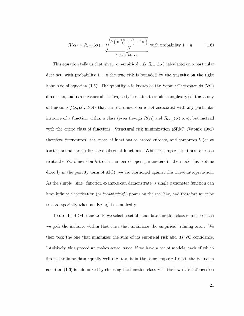
R(α) ≤ Remp(α) +

√h(ln 2N

h + 1)− ln η

4

N︸ ︷︷ ︸VC confidence

with probability 1− η (1.6)

This equation tells us that given an empirical risk Remp(α) calculated on a particular

data set, with probability 1 − η the true risk is bounded by the quantity on the right

hand side of equation (1.6). The quantity h is known as the Vapnik-Chervonenkis (VC)

dimension, and is a measure of the “capacity” (related to model complexity) of the family

of functions f(x,α). Note that the VC dimension is not associated with any particular

instance of a function within a class (even though R(α) and Remp(α) are), but instead

with the entire class of functions. Structural risk minimization (SRM) (Vapnik 1982)

therefore “structures” the space of functions as nested subsets, and computes h (or at

least a bound for it) for each subset of functions. While in simple situations, one can

relate the VC dimension h to the number of open parameters in the model (as is done

directly in the penalty term of AIC), we are cautioned against this naıve interpretation.

As the simple “sine” function example can demonstrate, a single parameter function can

have infinite classification (or “shattering”) power on the real line, and therefore must be

treated specially when analyzing its complexity.

To use the SRM framework, we select a set of candidate function classes, and for each

we pick the instance within that class that minimizes the empirical training error. We

then pick the one that minimizes the sum of its empirical risk and its VC confidence.

Intuitively, this procedure makes sense, since, if we have a set of models, each of which

fits the training data equally well (i.e. results in the same empirical risk), the bound in

equation (1.6) is minimized by choosing the function class with the lowest VC dimension

21

(or complexity). Note that the bound is a probabilistic bound (i.e. it is true with

probability 1− η), and is thus related to what is known as a Monte Carlo method in the

field of randomized algorithms (Motwani & Raghavan 1995). If the bound is tight for at

least one of the candidate function classes, then we are guaranteed that we can do no

better, but if the bound is not tight for any class under consideration, then we can do no

better than to hope for the best.

This relatively abstract notion serves as the basis for the highly popular support

vector machine (SVM). The SVM is a linear classifier, which finds a hyperplane that

(for linearly separable problems) maximally separates the two classes (which is why this

class of methods is also known as maximum-margin methods). For problems which are

not linearly separable, there exist variants (C-SVM and ν-SVM) which feature a tradeoff

parameter which allows simpler decision boundaries, at the expense of some training

classification errors. Interestingly, all inference in the SVM can be derived solely using

inner products in the data space. This allows us to easily extend its applicability to

nonlinear settings by the use of the kernel trick (Scholkopf & Smola 2000).

While the support vector machine is certainly considered to be a state-of-the-art ma-

chine learning tool, its inability to give true probabilistic predictions is a disadvantage. In

addition, the requirement of cross-validation to determine the correct values of the trade-

off parameter becomes prohibitively expensive for large data sets, and is not naturally

generalizable to online learning settings.

In general, the SRM framework does not explicitly deal with probability distribu-

tions over the hypothesis space, but only concerns itself with picking the correct function

(class) that minimizes the expected risk. It is difficult to map the framework of SRM

22

into equivalent notions in Bayesian statistical learning, or vice-versa. As such, it forms a

parallel body of work that is very effective at doing principled machine learning. While

proponents of the Bayesian methods value the flexibility of being able to introduce prior

knowledge about the hypothesis space, the SRM framework sidesteps the explicit model-

ing of probability distributions, since ultimately we are only concerned with the expected

error obtained by our learning machine.

1.4 Dissertation Outline

The remainder of this dissertation is organized as follows:

• Chapter 2 reviews graphical models as an intuitive tool for describing the prob-

abilistic relationships between variables in a statistical model. It discusses basic

inference techniques such as the junction tree algorithm for estimating marginal

distributions in such models, and highlights the analytical and computational dif-

ficulties that arise as the complexity of the models increase. We also discuss the

parameter optimization framework of expectation-maximization (EM), and show

that an elegant approximation technique known as the factorial variational approx-

imation can be derived very naturally as an extension.

• Chapter 3 introduces three algorithms contributed by this dissertation which tackle

especially difficult problems of model complexity estimation. The first deals with

estimating the cardinality of mixture models using a novel technique that approx-

imates the statistical evidence for splitting local models. The second algorithm

deals with the problem of estimating the size of the temporal “window” of sufficient

23

statistics in online learning problems. We show that by tracking the drifting process

using a variational Kalman smoother, we can obtain a principled estimate of this

window size. The third algorithm deals with estimating the spatial extent of locally

weighted learning components — a problem known as supersmoothing. We show

that by placing distributions over the kernel weighting parameters and by using

properties of convex duality to derive a lower bound, we can obtain a probabilistic

estimate of a local component’s spatial extent.

• Chapter 4 discusses the issue of the computational complexity of inference for su-

pervised learning. We review several efficient algorithms, some of which form the

inspiration for a novel derivation of backfitting — an efficient family of supervised

learning algorithms. By deriving backfitting with probabilistic underpinnings, we

can leverage the computational robustness of the original algorithm, while introduc-

ing the benefits of Bayesian inference and model selection. Using bounds derived

from convex duality, we extend the algorithm to classification tasks, and show that

the framework of sparse Bayesian learning can be derived using Bayesian backfitting

at its core. The popular relevance vector machine (RVM) is an example of such

an algorithm which can benefit from the scalability and robustness of Bayesian

backfitting.

• Chapter 5 concludes with a summary of the research presented in this thesis, and

a discussion of its future direction.

24

Chapter 2

The Quest for Analytical Tractability

In this chapter, we will briefly introduce graphical models, their types and the terminology

we will use to refer to them through the rest of this dissertation. We also review some

of the algorithms that are used to perform Bayesian inference in graphical models. In

particular, we will revisit the well-known expectation-maximization (EM) algorithm, and

show that an important class of approximate algorithms can be derived as a natural

generalization of this method.

2.1 Graphical Models

Probabilistic inference has been intimately tied to graph theory through the representa-

tion tool of graphical models (Pearl 1988, Lauritzen 1996). Given a graph G = (V, E), with

vertices V and edges E (directed or undirected), we associate a random variable x with

each vertex i ∈ V. The random variables may be discrete or continuous. Associated with

this graph, is a probability distribution over the set of random variables which factorizes

according to the structure of the graph. For discrete variables this distribution is a mass

function (a density with respect to a counting measure), while for continuous variables,

25

it is a density with respect to the Lebesgue measure. For any subset A ⊆ V we define

xA = xi|i ∈ A.

The structure of a graphical model imposes a factorization over the probability dis-

tribution, and elegantly captures the structure of conditional independence between the

variables in a statistical model. Variable xi is conditionally independent of another vari-

able y, given a third variable z, if we can write p(x, y|z) = p(x|z)p(y|z). Graphical models

representing the conditional independence relationships between random variables can be

broadly classified into two categories: undirected graphs (Markov networks or Markov

random fields), and directed acyclic graphs (DAGs, or Bayesian networks). The reader is

referred to (Lauritzen 1996) for an excellent formal treatise on graphical models in their

various representation forms.

In an undirected graphical model, we define a set of cliques C1 . . . CM to be a set of

maximally fully connected subsets of vertices in V, such that ∪Mm=1Cm = V. A clique Cm

is maximally fully connected if the addition of any vertex not already in Cm destroys the

fully connected property. In such a graphical model, the joint probability distribution

over the variables in the model is represented by a normalized product of clique potential

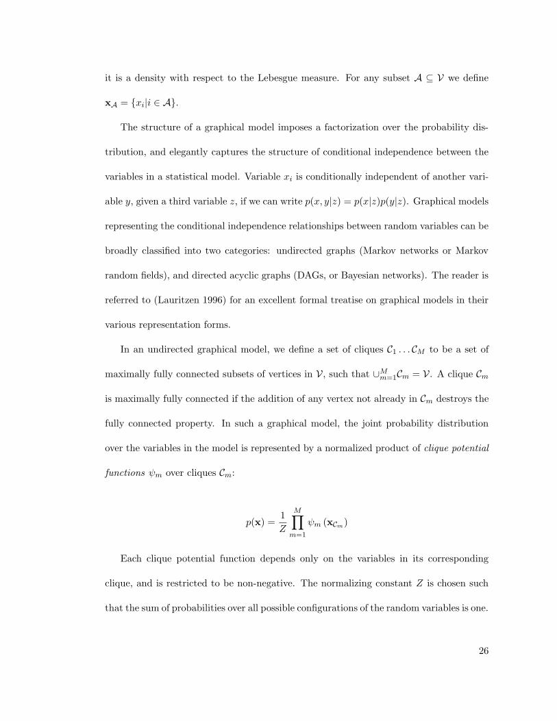
functions ψm over cliques Cm:

p(x) =1

Z

M∏

m=1

ψm (xCm)

Each clique potential function depends only on the variables in its corresponding

clique, and is restricted to be non-negative. The normalizing constant Z is chosen such

that the sum of probabilities over all possible configurations of the random variables is one.

26

Conditional independence in an undirected graphical model is represented by the concept

of graph separability. For three mutually disjoint sets of vertices A, B and C, we say that

xA and xB are conditionally independent given xC if all paths between a vertex in A and

another vertex in B must pass through a vertex in C (also known as the Markov property).

By the Hammersley-Clifford theorem (Hammersley & Clifford 1971), for strictly positive

density functions p(x), the factorization property across clique potentials, and the Markov

property are equivalent.

In a directed acylic graph, an edge from node xi to xj establishes that xi is the

parent of xj and equivalently, xj is the child of xi. If we denote by Pi the set of all

parents of vertex i, then the probability distribution over all variables in a graphical

model is represented by a product over conditional probability distributions over each

child variable given the set of its parents. Since the graph is acyclic, it establishes a

partial ordering over the variables, thus guaranteeing that this product is over a finite set

of terms:

p(x) =∏

i∈Vp (xi|xPi)

If we recursively define the descendents of a set of nodes to be the set of their children

and their children’s descendents, then the conditional independence that falls out of the

structure of a DAG is easily described: in a DAG, a set of variables is conditionally

independent of all its non-descendents given its parents.

Graphical models are a simple yet elegant tool for representing the structure of a

statistical model. As mentioned before however, we are primarily concerned with the

27

elimination of nuisance parameters from the statistical inference process, which can be

achieved using Bayesian inference. Unfortunately, using this framework often necessi-

tates an increase in the complexity of the graphical model, thus rendering it difficult or

impossible to derive analytically closed-form solutions to the posterior updates of the

unobserved variables in the model.

2.1.1 Graphical Model Conventions in this Dissertation

N

φ1 x1i

x3ix2

φ2

Figure 2.1: An example graphical model. This particular model is represented by adirected acyclic graph (DAG).

Figure 2.1 shows an example graphical model, which serves to illustrate some of the

conventions we will use throughout this dissertation when we use graphical models to

represent the structure of our statistical models.

1. Random variables in the model (x1, x2, and x3 in figure 2.1) will be drawn as

circular nodes. We will distinguish between observed and unobserved variables by

giving nodes corresponding to observed variables a double border. The collection of

these nodes is the observed data set xD = x1. We will typically be interested in

inferring marginal posterior distributions over the unobserved random variables. We

will collectively refer to these unobserved variables using the symbol xH = x2, x3.

28

2. Parameters which do not have distributions will be drawn as square nodes. We will

sometimes be interested in optimizing point estimates of these parameters such that

the model best fits the data. We will collectively refer to these parameters with the

symbol φ = φ1, φ2.

3. Edges in the graph are used to indicate dependencies between variables. A directed

edge from x2 to x1 implies that the distribution of x1 is conditioned on x2.

4. Repeated sets of variables (e.g. multiple samples from the same distribution) are

denoted by the use of a rectangular box around the variables called a plate. The vari-

ables inside the plate (x1 and x3 in figure 2.1) will typically have subscripts denoting

iteration over the repetitions. Unless otherwise specified, the variables in each copy

of the plate is conditionally i.i.d. (independently, identically distributed) given all

parent nodes outside the plate. In our example, this corresponds to x1i, x3i being

conditionally independent of x1j , x3j for j 6= i, given x2.

2.2 Inference in Graphical Models

Consider a graphical model represented by a graph G = (V, E), and let D,H be a

partition over V such that the random variables xD associated with the nodes in partition

D are observed, while the random variables xH in H are hidden. Additionally we consider

a set of variables φ which parameterize the distributions in the graphical model, or

otherwise relate to model structure and complexity. Importantly we assume that these

variables φ are not modeled as random variables, but rather as fixed parameters for which

we would like an estimate (such as the choice of model complexity).

29

Given a data set xD of observations corresponding to observed nodes in the model D,

we can classify our inferential requirements of a graphical model into two main categories:

1. Inference of the posterior distributions over the unobserved variables p(xH|xD;φ)

given the observed data and a particular setting of the parameters φ.

2. Optimization of the parameters φ such that the model best explains the observed

data, i.e. maximizes p(xD;φ).

2.2.1 Inferring Marginal Distributions

Although most of this dissertation will deal with statistical models that are represented

by DAGs, we will review inference in undirected graphs (Markov networks) since this

turns out to be a more general framework for inference in graphical models which can

then be applied to DAGs as well.

a

b

d

f

ec

(a) Directed acyclic graph

a

b

d

f

ec

(b) Resulting moralized MRF

Figure 2.2: The process of converting a DAG into an MRF proceeds by making sure thatthe parents Pi of each node i are connected — a process called moralization

30

A DAG can be converted into an undirected graph by the process of moralization.

For each node i ∈ V, we connect its parents Pi and remove direction from all edges

involved. Figure 2.2(b) shows the moralized undirected graph corresponding to the DAG

in figure 2.2(a). The additional edge (b, e) was added by moralizing the parents of node f .

Moralization ensures that the “explaining away” property of a fan-in in a belief network

is preserved in the resulting Markov network.

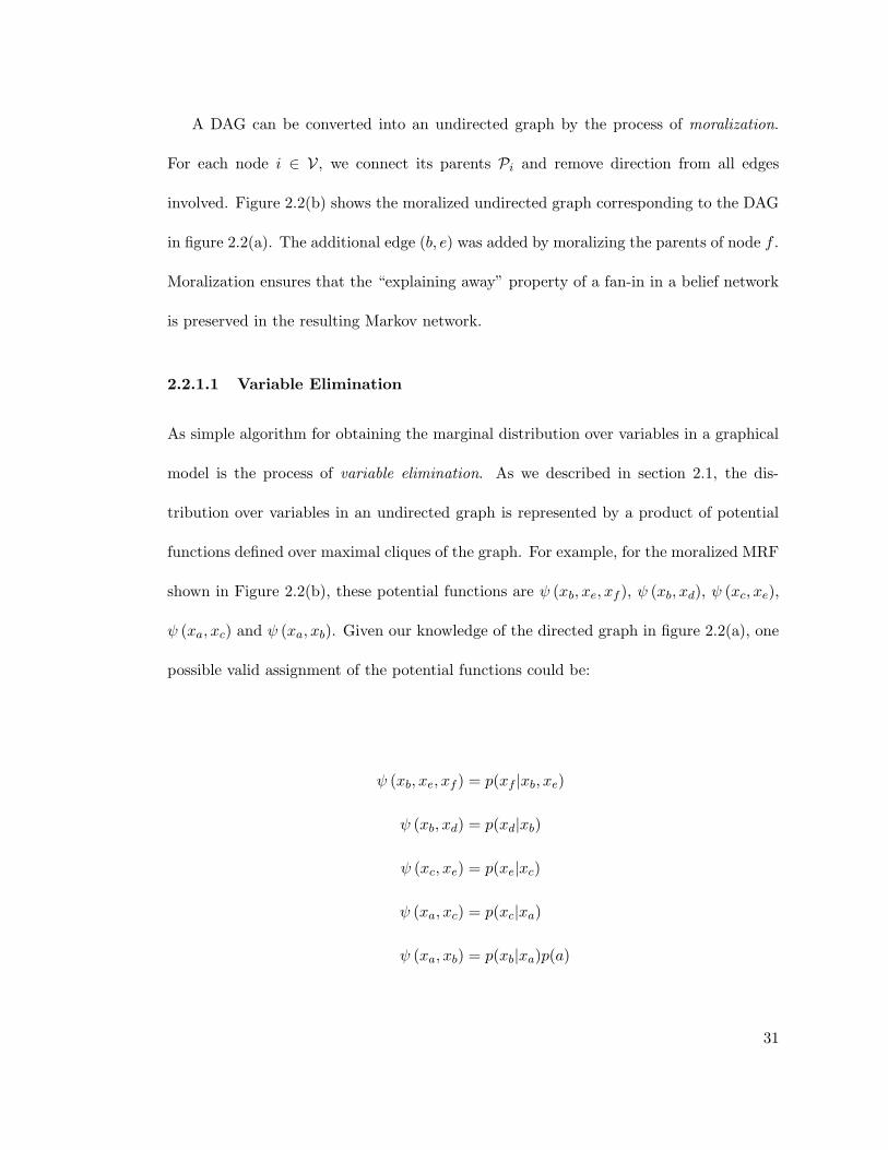
2.2.1.1 Variable Elimination

As simple algorithm for obtaining the marginal distribution over variables in a graphical

model is the process of variable elimination. As we described in section 2.1, the dis-

tribution over variables in an undirected graph is represented by a product of potential

functions defined over maximal cliques of the graph. For example, for the moralized MRF

shown in Figure 2.2(b), these potential functions are ψ (xb, xe, xf ), ψ (xb, xd), ψ (xc, xe),

ψ (xa, xc) and ψ (xa, xb). Given our knowledge of the directed graph in figure 2.2(a), one

possible valid assignment of the potential functions could be:

ψ (xb, xe, xf ) = p(xf |xb, xe)

ψ (xb, xd) = p(xd|xb)

ψ (xc, xe) = p(xe|xc)

ψ (xa, xc) = p(xc|xa)

ψ (xa, xb) = p(xb|xa)p(a)

31

allowing us to write the joint probability distribution as a product of potentials:

p(x) = ψ (xb, xe, xf )ψ (xb, xd)ψ (xc, xe)ψ (xa, xc)ψ (xa, xb)

To obtain the marginal probability of a single variable xi in the graphical model,

it suffices to choose an ordering of the remaining variables for “elimination” which is

equivalent to summing or integrating them out of the model. As each node in the sequence

is eliminated, it creates a dependency between its neighbors which is reflected by our

addition of edges between all neighbors of the eliminated node at each step.

Figure 2.3 shows the sequence of elimination steps for an elimination ordering of

f, e, d, c, a. Mathematically the sequence of eliminations is equivalent to the following

summations:

p(xb) =∑

xa

ψ (xa, xb)∑

xc

ψ (xa, xc)∑

xd

ψ (xb, xd)∑

xe

ψ (xc, xe)∑

xf

ψ (xb, xe, xf ) (2.1)

=∑

xa

ψ (xa, xb)∑

xc

ψ (xa, xc)∑

xd

ψ (xb, xd)∑

xe

ψ (xc, xe)mf (xb, xe)

=∑

xa

ψ (xa, xb)∑

xc

ψ (xa, xc)me (xb, xc)∑

xd

ψ (xb, xd)

= md (xb)∑

xa

ψ (xa, xb)∑

xc

ψ (xa, xc)me (xb, xc)

= md (xb)∑

xa

ψ (xa, xb)mc (xa, xb)

32

b

d

f

ec

a a

b

d

ec

a

c

b

d

a

b

c a

b

Figure 2.3: Each step in variable elimination picks a node, connects its neighbors, andmarginalizes that node out from the graph. In the figure, the sequence of eliminatednodes is f, e, d, c, a. The shaded region indicates the elimination clique created by thenode eliminated at each step. The dashed edge is introduced during the elimination ofnode e which requires that we connect its neighbors.

= md (xb)ma (xb)

The shaded region in each step of figure 2.3 is the elimination clique associated with

the node being eliminated. This set contains all the nodes involved in the summation at

that step in the elimination. Incorporating observed data into the elimination algorithm

is easy. For each observed variable xi where i ∈ D, we simply instantiate it in all the

potential functions in which xi appears. Summing over an evidence variable now reduces

to a single term.

33

a

b

d

f

ec

(a) Triangulated MRF

b, e, fb, c, ea, b, c b, eb, c

b, d

b

m3(b

)

m4(b

)

m2(b, c)

m5(b, c) m6(b, e)

m1(b, e)

(b) Junction tree with sequence of messages

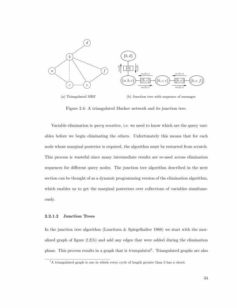
Figure 2.4: A triangulated Markov network and its junction tree.

Variable elimination is query sensitive, i.e. we need to know which are the query vari-

ables before we begin eliminating the others. Unfortunately this means that for each

node whose marginal posterior is required, the algorithm must be restarted from scratch.

This process is wasteful since many intermediate results are re-used across elimination

sequences for different query nodes. The junction tree algorithm described in the next

section can be thought of as a dynamic programming version of the elimination algorithm,

which enables us to get the marginal posteriors over collections of variables simultane-

ously.

2.2.1.2 Junction Trees

In the junction tree algorithm (Lauritzen & Spiegelhalter 1988) we start with the mor-

alized graph of figure 2.2(b) and add any edges that were added during the elimination

phase. This process results in a graph that is triangulated 1. Triangulated graphs are also

1A triangulated graph is one in which every cycle of length greater than 3 has a chord.

34

known as chordal graphs, and form a subset of graphical models in which both directed

and undirected graphical models have the same expressive power to represent statistical

relationships (Pearl 1988). From the maximal cliques of this triangulated graph, we can

create its cluster tree representation, by connecting the cliques via separator nodes. A

separator node between cliques Ci and Cj contains Ci ∩ Cj . A cluster tree is a junction

tree if for any pair of cluster nodes Ci and Cj , all nodes (cluster and separator) on the

path between Ci and Cj all contain Ci∩Cj . This is also known as the running intersection

property. One can show that the triangulation step ensures that the running intersection

property holds and that the cluster tree formed is indeed a junction tree. Figure 2.4

shows a junction tree corresponding to the triangulated moral graph from the previous

section. It is easy to verify its running intersection property. We define potentials over the

clique nodes in this new graph: ψ (xb, xe, xf ), ψ (xb, xc, xe), ψ (xa, xb, xc) and ψ (xb, xd).

In addition, we also have potentials over the variables in the separator nodes: ψ (xb, xe),

ψ (xb, xc) and ψ (xb).

Inference in a junction tree proceeds as follows:

• Choose a clique node as the root. In figure 2.4(b) we choose the root to be the node

representing clique a, b, c.

• Pass messages from leaf-nodes up towards the root, and then from the root back

down to the leaves. A message from clique Ci to an adjacent clique Cj is a two-step

update of the potential of a separator node Sij , as well as the destination clique

node Cj :

35

ψ∗(xSij

)=

∑

xCi\Sij

ψ (xCi)

ψ∗(xCj)

= ψ(xCj) ψ∗

(xSij

)

ψ(xSij

)

• The algorithm terminates when each edge in the graph has transmitted a message

exactly once in each direction. At this point, the potential at each cluster is the

marginal distribution over the variables in that cluster, i.e. ψ (xCi) = p(xCi).

Note that the maximal cliques nodes in the junction tree of figure 2.4(b) are the same

elimination cliques we observed formed during the variable elimination method (c.f. figure

2.3). Also, our notation for the intermediate terms in equation (2.1) is no coincidence.

Messages m1, m2 and m3 in figure 2.4(b) are identical to the intermediate terms mf ,

me and md respectively, in the elimination algorithm. While these messages allow us to

compute the marginals in the root clique (including p(xb) in the elimination example),

the remaining messages m4, m5, and m6 allow the marginals in the other cliques to be

obtained as well.

The computational complexity of the junction tree method depends heavily on the

structure of the graphical model, and the particular tree structure chosen. This in turn

depends on the edges added in the triangulation step. In general, finding the optimal

triangulation and tree structure is an NP-hard problem. For a junction tree with discrete

variables, the computational complexity is exponential in the size of the largest clique

node (also known as tree width), which stems from having to iterate over a possibly large

36

number of states for each variable. For continuous variables, the summation is replaced

by integration over the state space, which — depending on the form of the distributions

involved — may be analytically intractable.

2.2.1.3 Monte Carlo Methods

An alternative to approximating the posterior distributions in a statistical model is to

produce a representation composed of samples from these distributions. Monte Carlo

methods are computational techniques that seek to carry out probabilistic inference us-

ing representative sets of samples from probability distributions. There are two main

problems that demand attention when using sampling methods. Firstly, the distribu-

tion of interest must be sampled from. Several methods exist such as importance sam-

pling (Rubin 1988), which relies on an importance distribution which can be sampled

from easily. An alternative is to construct a Markov chain having the distribution of

interest as its stationary distribution. The Metropolis-Hastings algorithm (Metropolis

et al. 1953, Hastings 1970), and Gibbs sampling (Geman & Geman 1984) are two exam-

ples of this approach. MacKay (2003a) and Fearnhead (1998) provide a succinct review

of several sampling strategies.

An interesting subset of research in the sampling community has been that of sequen-

tial sampling methods, also known as particle filters. It is well known that Kalman filters

(Kalman 1960) are a simplification of the general Bayesian state estimation problem in

which the state and observation equations are assumed linear with Gaussian distribu-

tions. The seminal paper of Gordon, Salmond & Smith (1993) showed that by creative

use of importance sampling, one could relax the linear and Gaussian assumptions and

37

still retain the sequential nature of the algorithm. Doucet, de Freitas & Gordon (2001)

provide a comprehensive summarization of the current state of theoretical and practical

sequential state estimation research. One of the very successful applications of this set

of statistical tools is in creating solutions to the simultaneous localization and mapping

(SLAM) problem in mobile robotics (Thrun 2002). Recently Deutscher, Blake & Reid

(2000) have demonstrated the use of this technique for motion capture applications as

well.

2.2.2 Parameter Estimation and the EM Algorithm

The algorithms described in the preceding section allowed us to compute marginal distri-

butions over sets of variables in a graphical model. Frequently however, we are also often

interested in optimizing the parameterization φ of the model itself such that we are most

likely to generate our observations xD. This most naturally expressed as a maximization

of the marginal likelihood function (or evidence) p(xD;φ), and is appropriately called the

maximum likelihood (ML) framework.

Within the ML framework it is customary to refer to the quantity p(xD;φ) as the

incomplete likelihood since it assumes that only a subset of the nodes in the model

corresponding to xD are observed. In contrast the quantity p(xD,xH;φ) is called the

complete likelihood, since we must assume that the values of the hidden variables xH are

known as well.

Given our observations xD, the graph structure, and the mathematical form of the

probability distributions over the random variables, we require to find the parameter

38

value that maximizes the incomplete likelihood φ∗ = arg maxφ p(xD;φ). Note that this

is typically a non-trivial task for the following reasons:

1. As we discussed in section 2.2, the quantity p(xD;φ) is sometimes difficult to obtain

since it involves marginalization over the hidden variables xH:

p(xD;φ) =

∫p(xD,xH;φ)dxH =

∫p(xD|xH;φ)p(xH;φ)dxH (2.2)

2. Even when the marginal is analytically expressed, the subsequent optimization of

the parameters φ requires solving:

∂p(xD;φ)

∂φ= 0

In all but the most trivial models, the parameters φ are inextricably linked, thus

making an analytical expression for the optimal parameters purely in terms of the

observed variables xD impossible. A well-known example of this is the simple model

of density estimation using a mixture of Gaussians.

The expectation-maximization (EM) algorithm of Dempster, Laird & Rubin (1977)

is a parameter optimization algorithm that operates within the framework of ML param-

eter estimation. Due to the conditional independencies induced by the graphical model

structure, it is much more convenient to express the complete likelihood p(xD,xH;φ)

(as a product of conditional distributions or clique potentials) than it is to compute the

marginalized likelihood integral of equation (2.2). The important contribution of the EM

algorithm is the ability to perform the optimization of the model parameters φ, while still

39

working with the analytical convenience of the complete likelihood p(xD,xH;φ). While

several derivations of the EM algorithm exist, we shall briefly summarize one which relies

on creating a lower bound to the incomplete likelihood using Jensen’s inequality. As we

shall show in the next section, this particular route is an interesting precursor to an elegant

variational approximation technique known as the factorial variational approximation.

Given a partition of the vertices in the graph into observed and unobserved setsD,H,

let us hypothesize the existence of an arbitrary distribution Q(xH) over the unobserved

variables xH, which allows us to derive the following lower bound on the incomplete log

likelihood2:

ln p(xD;φ) = ln

∫p(xD,xH;φ)dxH

= ln

∫Q(xH)

[p(xD,xH;φ)

Q(xH)

]dxH

≥∫Q(xH) ln

[p(xD,xH;φ)

Q(xH)

]dxH (Jensen’s inequality) (2.3)

= 〈ln p(xD,xH;φ)〉Q +H [Q]

= F(Q,φ) (2.4)

where 〈·〉Q denotes expectation with respect to the distribution Q, and H [Q] denotes its

entropy. A crucial element of the functional lower bound F(Q,φ) in equation (2.4), is

that for the special case in which the distribution Q(xH) = p(xH|xD;φ) (the posterior

distribution of the hidden variables under the current parameter settings), the lower

2Maximizing the logarithm of the likelihood is justified due to the monotonic nature of the logarithm.In addition, it will facilitate the use of Jensen’s inequality — ln 〈x〉 ≥ 〈lnx〉 — in deriving the bound.

40

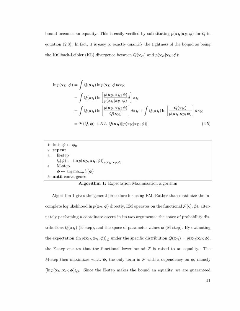
bound becomes an equality. This is easily verified by substituting p(xH|xD;φ) for Q in

equation (2.3). In fact, it is easy to exactly quantify the tightness of the bound as being

the Kullback-Leibler (KL) divergence between Q(xH) and p(xH|xD;φ):

ln p(xD;φ) =

∫Q(xH) ln p(xD;φ)dxH

=

∫Q(xH) ln

[p(xD,xH;φ)

p(xH|xD;φ)d

]xH

=

∫Q(xH) ln

[p(xD,xH;φ)

Q(xH)

]dxH +

∫Q(xH) ln

[Q(xH)

p(xH|xD;φ)

]dxH

= F (Q,φ) +KL [Q(xH)||p(xH|xD;φ)] (2.5)

1: Init: φ← φ0

2: repeat3: E-step

lc(φ)← 〈ln p(xD,xH;φ)〉p(xH|xD;φ)

4: M-stepφ← arg maxφ lc(φ)

5: until convergence

Algorithm 1: Expectation Maximization algorithm

Algorithm 1 gives the general procedure for using EM. Rather than maximize the in-

complete log likelihood ln p(xD;φ) directly, EM operates on the functional F(Q,φ), alter-

nately performing a coordinate ascent in its two arguments: the space of probability dis-

tributions Q(xH) (E-step), and the space of parameter values φ (M-step). By evaluating

the expectation 〈ln p(xD,xH;φ)〉Q under the specific distribution Q(xH) = p(xH|xD;φ),

the E-step ensures that the functional lower bound F is raised to an equality. The

M-step then maximizes w.r.t. φ, the only term in F with a dependency on φ; namely

〈ln p(xD,xH;φ)〉Q. Since the E-step makes the bound an equality, we are guaranteed

41

that maximizing F in the M-step also increases the incomplete log likelihood ln p(xD;φ).

Under general conditions (Wu 1983), EM is guaranteed to converge to a local maximum

in the incomplete likelihood p(xD;φ).

Several variants of the EM algorithm exist. To address computational issues, Neal

& Hinton (1998) have theoretically justified incremental and sparse variants, in which

only a subset of the hidden variables and/or parameters are updated in each EM cycle.

There also exist variants that seek to overcome the problem of local minima, such as

Deterministic Annealing EM (DAEM) (Ueda & Nakano 1998), and in the context of

mixture models, Split-and-Merge EM (SMEM) (Ueda et al. 1999). Minagawa et al.

(2002) showed however, that the SMEM mechanism may actually settle on suboptimal

solutions.

It is important to realize that the efficacy of the M-step depends upon being able to

successfully compute the expectation of the complete log likelihood ln p(xD,xH;φ) with

respect to the true posterior p(xH|xD;φ). This is because only the true posterior raises

the bound of equation (2.4) to an equality, and thereby guarantees that the M-step is

actually maximizing p(xD;φ) — the quantity of interest.

What happens when we cannot express the posterior p(xH|xD;φ) analytically? Or

when the required E-step expectation 〈ln p(xD,xH;φ)〉 with respect to this posterior is

intractable? This is where the realm of approximation methods plays a crucial role. In

the next section, we will derive an approximation method that stems naturally from the

EM formulation that we have just described.

42

2.3 The Factorial Variational Approximation

Often in statistical models, the marginal posterior distributions over variables is analyt-

ically intractable due to the structure of the individual conditional distributions. Even

using the junction tree methods of section 2.2 does not help since propagating and absorb-

ing messages involves the marginalization of variables in the cliques, which pose the same

analytical restrictions. Additionally exacerbating the problem is the process of variable

elimination, which typically adds additional dependency relations in the graph, further

complicating subsequent marginalizations.

An alternative way of addressing the issue is to make the a priori assumption that the

posterior distribution factorizes over certain sets of variables in the model (Beal 2003).

In some sense, this can be thought of as artificially restricting the clique size in the

junction tree of section 2.2.1.2. We can then restrict our search to families of posterior

distributions that satisfy this constraint. This approximation is therefore known as the

factorial variational approximation.

2.3.1 An Update Mechanism for Factored Posterior Distributions

Let us start with the lower bound derived in equation (2.4) of the preceding section:

ln p(xD;φ) ≥∫Q(xH) ln

[p(xD,xH;φ)

Q(xH)

]dxH

= 〈ln p(xD,xH;φ)〉Q +H [Q]

43

We know that maximizing the lower bound implies maximizing the functional F(Q,φ)

over the space of probability distributions Q(xH). Another way of formulating the prob-

lem is by noting that the tightness of the bound is quantified by the KL divergence

between the true posterior and its approximation, as shown in equation (2.5). This KL

divergence is also known as the variational free energy. Minimizing this free energy is

equivalent to tightening the lower bound, and bringing the approximation Q(xH) closer

to the true posterior p(xH|xD;φ). Moreover, we know that this a constrained variational

optimization problem since we must maintain that∫Q(xH)dxH = 1 over the space of

possible solutions.

If we do not impose any additional constraints, maximization of F(Q,φ) w.r.t. Q(xH)

will lead to the true posterior distribution p(xH|xD;φ) which we have assumed is analyt-

ically intractable. If however, we impose the additional constraint that the distribution

Q(xH) must factorize over some partitionxH1,xH2, . . . ,xHp

, i.e.:

Q(xH) =

p∏

i=1

Qi(xHi)

then using the calculus of variations (see (Rustagi 1976) for example,) we can derive

(see appendix B.1) the following update equation for the marginal posterior over each

individual partition xHi:

Qi(xHi) =exp 〈ln p(xD,xH;φ)〉Qk 6=i∫

exp 〈ln p(xD,xH;φ)〉Qk 6=i dxHi(2.6)

44

or equivalently:

lnQi(xHi) = 〈ln p(xD,xH;φ)〉Qk 6=i + constxHi (2.7)

where 〈·〉Qk 6=i denotes expectation taken w.r.t. all distributions Qk except Qi. This is a

particularly appealing formulation, since it allows us (once again) to work with the com-

plete joint distribution over our statistical model as we did before in the EM algorithm,

without the need for explicit marginalization. Successive application of the update (2.6)

to each distribution Qi(xHi) for 1 ≤ i ≤ p guarantees that each update monotonically

decreases the KL divergence between the approximated (factored) posterior Q(xH) and

the true posterior p(xH|xD;φ).

2.3.2 Solution for Partial Factorization

If we drop the assumption of complete factorization and allow dependencies between par-

titions then our result changes only slightly (see appendix B.1.1). Assume, for example,

that Q(xH1,xH2) = Q(xH1|xH2)Q(xH2). In this case, the update equations for Q(xH2)

become:

Q2(xH2) ∝ exp

(〈ln p(xD,xH;φ)〉Qj 6=2

−∫Q(xH1|xH2) lnQ(xH1|xH2)dxH1

)(2.8)

45

or equivalently

lnQ2(xH2) = 〈ln p(xD,xH;φ)〉Qj 6=2+ entropy Q(xH1|xH2)+ constxH2

(2.9)

The factorial variational approximation has only recently gained attention in the

machine learning community although it has its roots in statistical physics and mean

field theory (Parisi 1988). MacKay (1999) provides an insightful comparison of these so-

called approximating ensemble methods with the traditional exact methods, and shows

that in cases where we are inclined to summarize the posterior distributions with point

estimates, ensemble methods are a more accurate representation of the location of overall

posterior mass.

The analytical simplicity of the variational approximation has found several applica-

tions in the statistical learning literature. Saul, Jaakkola & Jordan (1996) use a mean

field approximation to create tractable inference in sigmoid belief networks. Ghahramani

& Beal (2000) have extended probabilistic factor analysis (FA) models (Ghahramani &

Hinton 1997) to incorporate automatic estimation of the number of latent dimensions.

Identical formulations have also been presented in the context of principal component

analysis (PCA) (Bishop 1999b, Bishop & Winn 2000). Ghahramani & Beal (2001) also

show that the variational approximation can be used in the general case of conjugate-

exponential belief networks (i.e. models in which the conditional distributions are from

the exponential family, and whose priors are conjugate), as well as Markov networks. In

fact, it can be formulated as a form of message-passing or propagation algorithm similar

to the junction tree method described in section 2.2.1.2. They also demonstrate its use

46

in several statistical learning problems such as a Bayesian treatment of Kalman filter pa-

rameter estimation. Sato (2001) shows for the case of conjugate exponential models, that

one can use the variational approximation to derive posterior distributions that retain

their prior form, thus enabling observed data to be summarized by the sufficient statistics

of these distributions. Observing new data is then naturally incorporated into the model

by the update of these statistics, thus enabling efficient online learning implementations.

Other forms of variational approximations exist which do not necessarily include a

factorization. Variational calculus has been used to find the optimal parameterization of

a functional lower bound to a true posterior distribution in each node of sigmoid belief

networks (Saul et al. 1996, Jordan, Ghahramani, Jaakkola & Saul 1999). Prior to the use

of variational approximations, a popular method for approximating intractable distribu-

tions has been the Laplacian approximation (also known as the Gaussian approximation),

which uses a second-order Taylor series expansion at the maximum of the distribution

(Bishop 1999a). The Hessian matrix of the quadratic surface at the location of the max-

imum serves as the covariance matrix of the Gaussian approximation. Gelman et al.

(1995) present several asymptotic justifications for this approach, as well as counterex-

amples where it does not work well. Wainwright & Jordan (2003) show that by using the

theory of convex duality, one can derive several approximate inference algorithms, includ-

ing the factorial variational approximation, loopy belief propagation, and Bethe/Kikuchi

approximations.

47

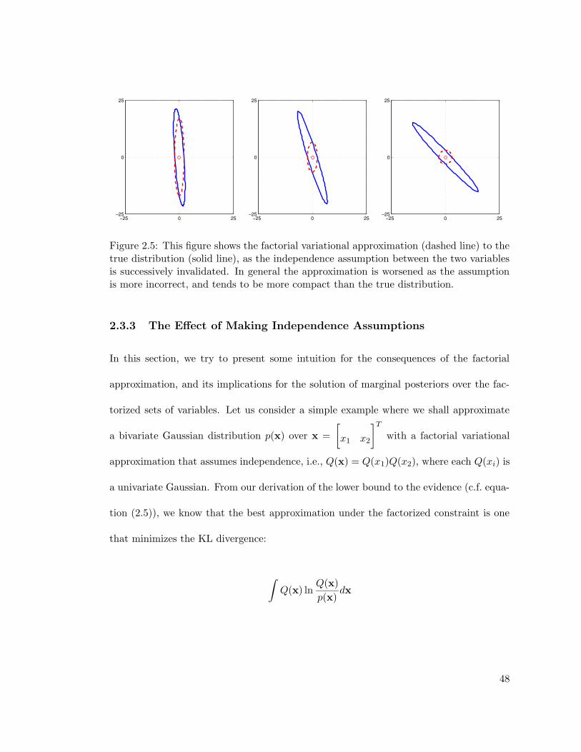
−25 0 25−25

0

25

−25 0 25−25

0

25

−25 0 25−25

0

25

Figure 2.5: This figure shows the factorial variational approximation (dashed line) to thetrue distribution (solid line), as the independence assumption between the two variablesis successively invalidated. In general the approximation is worsened as the assumptionis more incorrect, and tends to be more compact than the true distribution.

2.3.3 The Effect of Making Independence Assumptions

In this section, we try to present some intuition for the consequences of the factorial

approximation, and its implications for the solution of marginal posteriors over the fac-

torized sets of variables. Let us consider a simple example where we shall approximate

a bivariate Gaussian distribution p(x) over x =

[x1 x2

]Twith a factorial variational

approximation that assumes independence, i.e., Q(x) = Q(x1)Q(x2), where each Q(xi) is

a univariate Gaussian. From our derivation of the lower bound to the evidence (c.f. equa-

tion (2.5)), we know that the best approximation under the factorized constraint is one

that minimizes the KL divergence:

∫Q(x) ln

Q(x)

p(x)dx

48

Figure 2.5 shows the resulting approximation for different distributions p(x) which

have increasing degrees of dependence between x1 and x2. MacKay (2003b) points out

that the variational approximation will always tend to produce more compact distri-

butions than the true posterior. This is also evident in figure 2.5 where the resulting

approximation tends to put most of the probability mass on the subset of the domain

which has support under both the true posterior distribution and the approximation.

Interestingly, MacKay (2003b) notes that if we instead minimize the following KL

divergence:

∫p(x) ln

p(x)

Q(x)dx

we get the opposite effect, in which the resulting approximation tends to put most of the

probability mass on the superset of the domain which has support under the approxima-

tion and the true distribution (i.e. we obtain an axis-aligned Gaussian which encompasses

the true distribution), and thus obtain a less compact approximation.

The interesting question is what this result would seem to imply in terms of model

complexity estimation. A more compact distribution may seem to suggest that the model

overfits since it gives higher probability than it should to a particular solution. However,

it should be noted that whether this behavior corresponds to overfitting or underfitting

depends on the space of models that is given high probability in the posterior. If a

compact approximation puts more probability mass on the subspace of models which

have lower complexity then we would in fact have the effect of underfitting the model

since the true complexity cannot be accurately represented with our approximation.

49

Additional support for this idea of underfitting is given by MacKay (2001), who notes

that in the presence of fewer data points, variational approximations tend to prune away

additional model complexity, and require large amounts of data to justify retaining more

complex models.

As a last point, it should be mentioned that certain dependencies in a statistical

model take the form of symmetries in the parameter space; for example, permutations of

mixture component labels and parameters. The joint posterior distributions are therefore

notoriously multimodal. By neglecting these dependencies, the factorial variational ap-

proximation will settle on one of the modes, but the choice of mode is highly dependent

on initialization of the inference process. In situations like mixture modeling for example,

this is typically not a problem since from a model evidence point of view, the solutions

at all the symmetric modes are equivalent.

50

Chapter 3

Algorithms for Analytical Tractability

Armed with the analytical methodology presented in chapter 2, and in particular, the

framework of variational approximations, we seek to tackle some of the particularly dif-

ficult problems that require a careful consideration of model complexity in order for

inference to be successful. Section 3.1 develops a novel algorithm that addresses the issue

of determining the appropriate number of components in mixture modeling. Using the

factorial variational approximation, we create a closed form solution to the problem of

modeling local evidence, which allows us to grow a collection of mixture components to

suit the complexity of the data set.

In section 3.2 we deal with the problem of estimating the window of sufficient statistics

(or equivalently, the forgetting factor) used in online learning situations where we must

model a time-varying system. By modeling the parameters of the time-varying system

as a set of drifting parameters, we derive an algorithm that extends the Kalman filter

to determine the appropriate size of the window of sufficient statistics required in online

learning problems.

51

Finally, section 3.3 addresses the analogous problem of determining the spatial extent

of kernels in locally weighted learning — a problem also known in the statistics literature

as supersmoothing. By modeling the kernel weights probabilistically, we can achieve both

an automatic estimation of the kernel width, as well as gain robustness to outliers.

3.1 Mixture Model Cardinality

Mixture modeling (McLachlan & Peel 2000) is a well-established, powerful tool for mod-

eling complex data using a collection of simple, local models. It intuitively describes

situations in which each observation is modeled as having been produced by one of a

set of alternative mechanisms. This is not the only useful interpretation, however, since

mixtures of analytically simple distributions (such as Gaussians) can be used to model

arbitrarily complex density functions, and mixtures of computationally efficient locally

linear regressors can be used to fit arbitrarily nonlinear regression data. Thus mixture

modeling is also a useful tool of composition.

The optimization of model parameters in finite mixture models often seeks to maxi-

mize a measure of goodness of fit (or equivalently, minimize an error measure), between

the model and the observed data. This typically involves a joint optimization of the

parameters that define the locality of each model (for example, the parameters of the

gating network as used by Jordan & Jacobs (1994)), along with the parameters that fit

each local model to the data (for example, the parameters of a local factor analyzer or

local linear regression parameters).

52

If we merely wished to estimate the parameters of a collection of components of

known cardinality, then the problem can be tackled using the expectation-maximization

(EM) algorithm (Dempster et al. 1977) mentioned in section 2.2.2, and its many variants

(Neal & Hinton 1998, Ueda & Nakano 1998, Ueda et al. 1999), which provide a clean

optimization mechanism within the maximum likelihood (ML) framework. Estimating

the number of mixture components however, is an issue of determining the statistical

model complexity and is still a largely unsolved problem. It is well known that increasing

the number of mixture components monotonically increases the fit to the observed data (Li

& Barron 2001, Cadez & Smyth 2001), since each model with k+ 1 components contains

the k-component model as a special case, and consequently, must have a likelihood greater

than or equal to a k-component model. This increased likelihood, however, comes at a

price of poor generalization ability due to the increase in model complexity; another

manifestation of the classic bias-variance dilemma (Geman et al. 1992).

There have been various approaches to estimating and/or regularizing model com-

plexity with respect to the number of mixture components. Some have included eval-

uating the fitness function for various numbers of components and then performing a

statistical hypothesis test to determine the most appropriate complexity (Chuang &

Mendell 1997, Mendell et al. 1993). An alternative approach penalizes the fitness func-

tion with a term that scales with model complexity. The approaches discussed in sec-

tion 1.3 such as the minimum description length (MDL) principle (Rissanen 1978), and

Bayesian/Akaike information criteria (BIC/AIC) (Schwarz 1978, Akaike 1974, Roeder &

Wasserman 1995, Mengerson & Robert 1996) fall in this category.

53

Cross-validation for selecting the number of mixture components, although, in general,

computationally intensive, has also been attempted. Smyth (2000) compares a particu-

lar implementation of cross-validated methodologies called Monte Carlo cross validation

(MCCV) and compares it to other non-Bayesian approaches including BIC and bootstrap

methods. In addition, there are several non-parametric clustering methods (see, for ex-

ample, (Zhang & Liu 2002) and references therein) that also attempt to automatically

discover the number of clusters. One of the more exciting of these approaches has been

the use of semi-parametric Bayesian models and the family of Pitman-Yor processes to

model a countably infinite number of mixture components (Pitman & Yor 1997, Escobar

& West 1995, Ishwaran & James 2002). Solutions to these models however are obtained

via MCMC sampling techniques, and are prohibitively expensive for high-dimensional

data. For the remainder of this section, we shall restrict ourselves, however, to model-

based approaches, and attempt to derive an algorithm using the approximation techniques

mentioned in chapter 2.

There has already been some research that makes steps in this direction. In the

context of mixtures of factor analyzers, Ghahramani & Beal (2000) have used variational

calculus to approximate the model evidence, and hence successfully discover the local

dimensionality within each factor analyzer. Their approach to inferring the number of

model components, however, involves a heuristic which stochastically chooses a candidate

model for splitting based on its contribution to the overall (approximated) evidence.

The idea of using a local measure to determine a splitting criterion, however, is a

promising one. And it is this approach that we will explore in the remainder of this

section.

54

3.1.1 Growing Mixture Models

One possible solution to estimating the cardinality of a mixture model is to overestimate

the complexity by creating far more models than is necessary, and then allowing the

evidence maximization process to prune away the excess model complexity (Blei & Jordan

2004). Ideally however, we would like to use a growing rather than a pruning approach

to determining mixture model cardinality since this reduces the initial computational

burden, and removes the decision of the initial overestimate in the number of components.

3.1.1.1 1 or 2 Models?

As a starting point, consider the simple problem of deciding between one or two mixture

components given the observed data. Let us assume we have a data set xD = xiNi=1

consisting of d-dimensional input vectors xi. Our task is to model the probability dis-

tribution p(x) using either one, or two Gaussians (it is straightforward to modify the

following discussion such that it is applicable to classification or regression tasks). We

represent a K-component mixture of Gaussians by the following equations:

x|sim = 1 ∼ Normal(x;µm,P

−1m

)

si ∼ Multinomial (si;π)

p(x) =K∑

k=1

p(x|sik = 1)πk

(3.1)

In equations 3.1, each si is a K-component vector of indicator variables and π is a

vector of prior probabilities for each component. µm, and Pm represent the mean and

55

N 2

xi

R

u2

u1

Pm

ζ

si

µm

ν

Figure 3.1: This statistical model determines whether a local patch of data requires oneor two components to be modeled. By recursively splitting models, we hope to grow acollection of mixture components that best models the data with minimum complexity.

precision of the mth Gaussian for 1 ≤ m ≤ K. For our present discussion, we restrict

K = 2. If we use likelihood as a model fitness criterion, then it is obvious that the

2-Gaussian model will always have performance better-than or equal-to that of the 1-

Gaussian model (Cadez & Smyth 2001). If however, we compute the marginal likelihood,

and integrate over the parameters for each K-component model, then we should be able

to correctly determine the appropriate complexity required to model the data xD without

over fitting. This implies computing the integral for the model evidence:

p(xD;MK) =

∫p(xD|xH)p(xH;MK)dxH

We use xH to represent the collective set of model parameters that we must integrate

over. In order to compute the marginal evidence, we alter the statistical model by placing

the following prior distributions:

56

µm|Pm ∼ Normal(µm; 0,P−1

m /α0

)(3.2)

Pm ∼Wishartν (Pm; R) (3.3)

p(si1 = 1) = ζ and p(si2 = 1) = 1− ζ (3.4)

ζ ∼ Beta (ζ;u1, u2) (3.5)

In equations (3.2) and (3.3) we place a joint Normal-Wishart prior over µm,Pm.

Gelman et al. (1995) provide several justifications for this choice of joint prior. In addition,

as shown in equation (3.4), our indicator variable si is now just a binomially distributed

2-component vector

[si1 si2

]T, while we represent our uncertainty about the knowledge

of the binomial parameter with the Beta prior in equation (3.5). This model is graphically

represented by the DAG in figure 3.1.

The joint distribution over the variables in this model factorize according to the

structure in the graphical model as follows:

p(xD,xH;M2) =

[N∏

i=1

2∏

m=1

[p (xi|µm,Pm) p (sim = 1)]sim

][2∏

m=1

p(µm|Pm)p(Pm)

]p(ζ)

In order to compute the model evidence p(xD;M2), the collective set of parameters

that we have to integrate over is xH =µm,Pmm=1,2 , siNi=1 , ζ

. As mentioned be-

fore, this integral is analytically intractable, and although exact solutions can be found

57

using Markov Chain Monte Carlo (MCMC) (Neal 1994), we choose to find an analyti-

cal solution using the factorial variational approximation of section 2.3. We make the

following factorial assumption over the posterior distribution of unknown variables:

Q(xH) = Q(µ,P,S, ζ)

= Q(µ,P)Q(S)Q(ζ)

If we substitute the conditional distributions, take logarithms, and lump all irrelevant

terms into an additive constant, we get:

ln p(xD,xH;M2) =N∑

i=1

si1

[1

2ln |P1| −

1

2(xi − µ1)TP1 (xi − µ1) + ln ζ

]

+ si2

[1

2ln |P2| −

1

2(xi − µ2)TP2 (xi − µ2) + ln (1− ζ)

]

+∑

m=1,2

[d

2lnα0 +

1

2ln |Pm| −

α0

2µm

TPmµm

]

+∑

m=1,2

[(η − d− 1

2

)ln |Pm| −

1

2Tr[R−1Pm

]]

+ (u1 − 1) ln ζ + (u2 − 1) ln (1− ζ) + constxD,xH

(3.6)

Using the update equation for factored distributions in equation (2.6), we can de-

rive the following updates (see appendix B.2) to each of the marginal distributions that

maximize the functional lower bound to the true evidence:

58

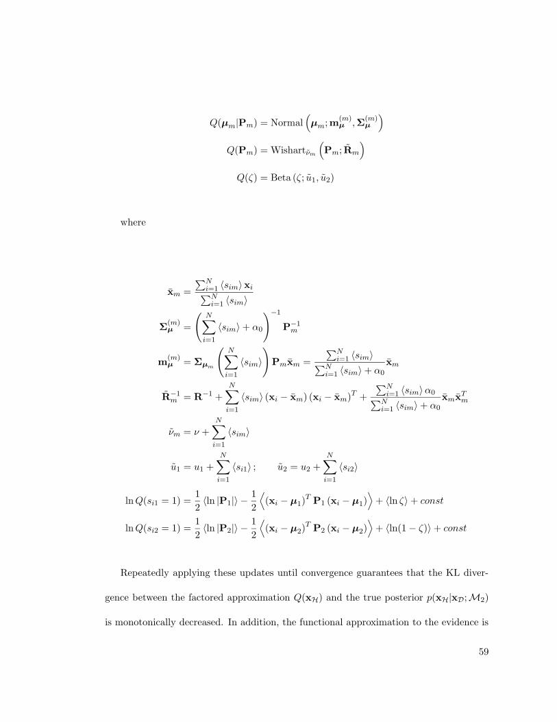
Q(µm|Pm) = Normal(µm; m

(m)µ ,Σ

(m)µ

)

Q(Pm) = Wishartνm

(Pm; Rm

)

Q(ζ) = Beta (ζ; u1, u2)

where

xm =

∑Ni=1 〈sim〉xi∑Ni=1 〈sim〉

Σ(m)µ =

(N∑

i=1

〈sim〉+ α0

)−1

P−1m

m(m)µ = Σµm

(N∑

i=1

〈sim〉)

Pmxm =

∑Ni=1 〈sim〉∑N

i=1 〈sim〉+ α0

xm

R−1m = R−1 +

N∑

i=1

〈sim〉 (xi − xm) (xi − xm)T +

∑Ni=1 〈sim〉α0∑N

i=1 〈sim〉+ α0

xmxTm

νm = ν +N∑

i=1

〈sim〉

u1 = u1 +N∑

i=1

〈si1〉 ; u2 = u2 +N∑

i=1

〈si2〉

lnQ(si1 = 1) =1

2〈ln |P1|〉 −

1

2

⟨(xi − µ1)T P1 (xi − µ1)

⟩+ 〈ln ζ〉+ const

lnQ(si2 = 1) =1

2〈ln |P2|〉 −

1

2

⟨(xi − µ2)T P2 (xi − µ2)

⟩+ 〈ln(1− ζ)〉+ const

Repeatedly applying these updates until convergence guarantees that the KL diver-

gence between the factored approximation Q(xH) and the true posterior p(xH|xD;M2)

is monotonically decreased. In addition, the functional approximation to the evidence is

59

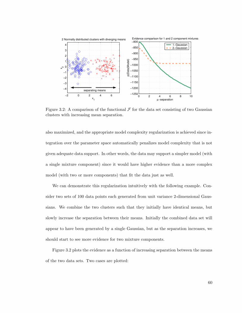
−2 0 2 4 6

−4

−3

−2

−1

0

1

2

3

4

x1

x 2

2 Normally distributed clusters with diverging means

0 2 4 6 8 10−1250

−1200

−1150

−1100

−1050

−1000

−950

−900

−850

−800

µ−separation

p(D

ata|

Mod

el)

Evidence comparison for 1 and 2 component mixtures

1−Gaussian2−Gaussian

separating means

Figure 3.2: A comparison of the functional F for the data set consisting of two Gaussianclusters with increasing mean separation.

also maximized, and the appropriate model complexity regularization is achieved since in-

tegration over the parameter space automatically penalizes model complexity that is not

given adequate data support. In other words, the data may support a simpler model (with

a single mixture component) since it would have higher evidence than a more complex

model (with two or more components) that fit the data just as well.

We can demonstrate this regularization intuitively with the following example. Con-

sider two sets of 100 data points each generated from unit variance 2-dimensional Gaus-

sians. We combine the two clusters such that they initially have identical means, but

slowly increase the separation between their means. Initially the combined data set will

appear to have been generated by a single Gaussian, but as the separation increases, we

should start to see more evidence for two mixture components.

Figure 3.2 plots the evidence as a function of increasing separation between the means

of the two data sets. Two cases are plotted:

60

• The solid line shows the evidence when the model is constrained to use only a single

Gaussian (by appropriately constraining its priors) to model the data. As expected,

the evidence monotonically decreases as the separation between the two clusters is

increased.

• The dashed line shows the evidence when the model is free to use two Gaussians.

Initially, although the 2-Gaussian model chooses to retain only a single Gaussian, its

evidence is lower due to its higher model complexity. As the separation increases

however, the 2-Gaussian case has enough evidence to warrant the existence of 2

components, after which its evidence stays essentially constant.

We also notice a distinct crossover point at which the evidence for the 2-Gaussian

model becomes higher than that of the 1-Gaussian model. This is a crucial observation

since we can effectively use the evidence (or in this case, the approximation F to the

evidence) as a distinction mechanism to make an automatic choice between using 1 or 2

Gaussians to model the given data.

We can now embed this result in a framework that provides us with a principled way

of increasing the number of models to account for structure in the data.

3.1.2 An Algorithm for Growing Mixture Model Cardinality

We are now in a position to formulate an algorithm based on the results of the pre-

vious section. Given a K-component mixture model, the 1-component v/s 2-component

decision that we discussed in the previous section can be applied to each of the K com-

ponents, to make a local decision about splitting a local model into 2 components. In

61

−0.5

0

0.5

1

−0.5

0

0.5

1

0

0.5

1

1.5

2

x1

x2

x 3

Figure 3.3: Starting with an initial set of 5 components, the model grows in complexityto settle on a final estimate of 14 components.

this way, starting with a very small number of components (or even a single component),

we can grow the number of components until the local evidence at each component votes

in favor of 1 model instead of 2. Algorithm 2 details this procedure.

Although in the previous section, we explicitly evaluated the evidence of the 1-

component and 2-component models separately, practically we only need to start with the

1: Init: K = 1, xH =µ1,P1, si1Ni=1 , ζ

2: repeat3: for m = 1 to K do4: Hypothesize an M2 model covering the same data xDm as component m5: Maximize p(xDm ;M2)6: if split then7: K ← K + 18: xH ← xH ∪

µK ,PK , siKNi=1

9: end if10: end for11: until no split occurs

Algorithm 2: Growing Mixture Models

62

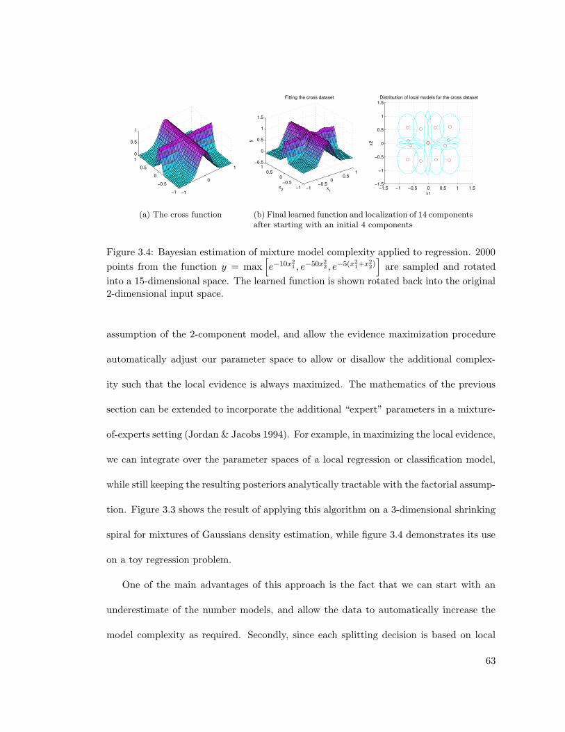
−1

0

1

−1

−0.5

0

0.5

10

0.5

1

(a) The cross function

−1−0.5

00.5

1

−1−0.5

00.5

1−0.5

0

0.5

1

1.5

x1

Fitting the cross dataset

x2

y

−1.5 −1 −0.5 0 0.5 1 1.5−1.5

−1

−0.5

0

0.5

1

1.5

x1

x2

Distribution of local models for the cross dataset

(b) Final learned function and localization of 14 componentsafter starting with an initial 4 components

Figure 3.4: Bayesian estimation of mixture model complexity applied to regression. 2000

points from the function y = max[e−10x2

1 , e−50x22 , e−5(x2

1+x22)]

are sampled and rotated

into a 15-dimensional space. The learned function is shown rotated back into the original2-dimensional input space.

assumption of the 2-component model, and allow the evidence maximization procedure

automatically adjust our parameter space to allow or disallow the additional complex-

ity such that the local evidence is always maximized. The mathematics of the previous

section can be extended to incorporate the additional “expert” parameters in a mixture-

of-experts setting (Jordan & Jacobs 1994). For example, in maximizing the local evidence,

we can integrate over the parameter spaces of a local regression or classification model,

while still keeping the resulting posteriors analytically tractable with the factorial assump-

tion. Figure 3.3 shows the result of applying this algorithm on a 3-dimensional shrinking

spiral for mixtures of Gaussians density estimation, while figure 3.4 demonstrates its use

on a toy regression problem.

One of the main advantages of this approach is the fact that we can start with an

underestimate of the number models, and allow the data to automatically increase the

model complexity as required. Secondly, since each splitting decision is based on local

63

evidence, the computation does not have to take into account the entire data set and hence

is efficient. Finally, the splitting decision is based on the much more principled criterion of

evidence maximization compared to previous approaches, which is guaranteed to locally

regularize model complexity.

One potential pitfall of this method is the phenomenon of “sudden death” which

happens when the complexity of the data covered by a single model is too great to

be modeled by just two components. In such a situation, both the 1-component and

2-component choices model the data equally badly resulting in the choice of a simpler

model (no split) to maximize evidence at the current level of (bad) fit. In such a case,

one solution would be to attempt a split into more than 2 components in regions where

the data distribution seems to warrant additional complexity. Reliably detecting these

situations is a topic of further research.

3.1.3 Application to Non-linear Latent Dimensionality Estimation

Recent research has provided increasingly more evidence for the existence of internal

models in biological motor control — either as forward models or inverse models. For

example, an inverse model of the body’s dynamics allows the generation of appropriate

muscle activations when supplied with a desired movement trajectory. In the most vision-

ary theories, internal models of the entire body dynamics and kinematics are required

to accomplish motor competence. However, from a statistical learning viewpoint, the

acquisition of such large internal models is very complex due to the hundreds of (possibly

irrelevant/redundant) input dimensions from various afferent and efferent sources — a

similar problem as that which seems to be solved by the mammalian cerebellum. Early

64

theories in computational motor control rejected internal model-based control due to the

daunting complexity of the differential equations that govern such models, and the high

dimensionality of the input spaces from which these models are learned.

From a control theoretic point of view, model-based feed-forward control has been

highly successful, particularly for fast movements with significant feedback loop delays.

In recent years however there has been mounting evidence (Kawato 1999) that internal

models are used in biological motor control (e.g., from force field experiments, neuro-

physiology of oculomotor control, lesion and clinical studies of the cerebellum). An open

theoretical research question is therefore: what is the complexity of the learning task

that needs to be tackled for motor control? Clearly, the hope is that even though the

movement system is extremely high-dimensional, kinematic and other constraints will

restrict movement data to reside in a very low dimensional manifold within this space,

thus providing a simpler learning task when expressed in terms of these low-dimensional

variables.

To answer this question, we performed a local dimensionality analysis of a significant

amount of movement data (D’Souza, Vijayakumar & Schaal 2001). If indeed, the data

was discovered to exist in locally low dimensional manifolds, then this would imply that

learning a model of movement data would only need to operate in this low dimensional

space — thus providing evidence that it is indeed feasible to learn internal models. The

data is analyzed using two statistical methods: singular value decomposition (SVD) and

our growing mixture model with each component being a variational Bayesian factor

65

α zi

xi

bα

aα

W

µ

Ψ

bψ

aψ

Σµ0µ0

Figure 3.5: Graphical model for Bayesian factor analysis.

analyzer (Ghahramani & Beal 2000). Bayesian factor analysis treats the latent dimen-

sionality of the model as an unknown model complexity parameter which must be esti-

mated. While several methods exist to estimate this latent dimensionality (Ghahramani

& Hinton 1997, Bishop 1999a, Bishop 1999b), we choose to extend the model presented

in (Ghahramani & Beal 2000) since it fits well with our variational scheme.

The graphical model for variational factor analysis is shown in figure 3.5. The observed

high-dimensional data x is assumed to be a linear combination W of a low-dimensional

set of latent variables z with additive axis-aligned noise:

xi = Wzi + µ+ ηi where ηi is i.i.d. Normal (ηi; 0,Ψ)

By placing priors over each column of W, we can regularize over the number of latent

variables that are required to reconstruct x. This model serves as a single component

66

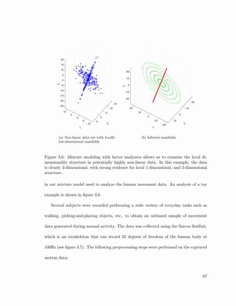
−10−5

05

10

−15

−10

−5

0

5

−25

−20

−15

−10

−5

0

5

10

15

20

t2

t1

t 3

(a) Non-linear data set with locallylow-dimensional manifolds

−20

−10

0

10

20

−20

−10

0

10

−20

−10

0

10

20

t2

t1

t 3

(b) Inferred manifolds

Figure 3.6: Mixture modeling with factor analyzers allows us to examine the local di-mensionality structure in potentially highly non-linear data. In this example, the datais clearly 3-dimensional, with strong evidence for local 1-dimensional, and 2-dimensionalstructure.

in our mixture model used to analyze the human movement data. An analysis of a toy

example is shown in figure 3.6.

Several subjects were recorded performing a wide variety of everyday tasks such as

walking, picking-and-placing objects, etc., to obtain an unbiased sample of movement

data generated during normal activity. The data was collected using the Sarcos SenSuit,

which is an exoskeleton that can record 35 degrees of freedom of the human body at

100Hz (see figure 3.7). The following preprocessing steps were performed on the captured

motion data:

67

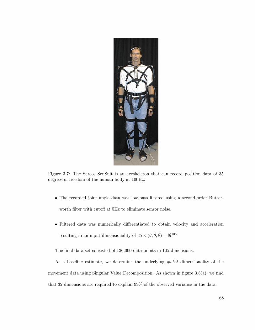
Figure 3.7: The Sarcos SenSuit is an exoskeleton that can record position data of 35degrees of freedom of the human body at 100Hz.

• The recorded joint angle data was low-pass filtered using a second-order Butter-

worth filter with cutoff at 5Hz to eliminate sensor noise.

• Filtered data was numerically differentiated to obtain velocity and acceleration

resulting in an input dimensionality of 35× (θ, θ, θ) = <105

The final data set consisted of 126,000 data points in 105 dimensions.

As a baseline estimate, we determine the underlying global dimensionality of the

movement data using Singular Value Decomposition. As shown in figure 3.8(a), we find

that 32 dimensions are required to explain 99% of the observed variance in the data.

68

(a) Estimation using SVD (b) Estimation with Bayesian mixtures of fac-tor analyzers

(c) Distribution of latent dimensionality

Figure 3.8: A histogram of the latent dimensionality of movement collected with theSenSuit. The weight of each bin is the ratio of the total amount of data that is modeledby a factor analyzer of that dimensionality.

In a sense, the global dimensionality estimate is the maximum that we can expect

the local dimensionality of the data to be. This figure however is an overestimate since it

fails to take into account local structure. By analyzing the same data set with mixtures

of Bayesian factor analyzers, we address the issue of local structure, as well as create a

mathematically principled estimate of local dimensionality within each model. As shown

in figure 3.8(b), when local structure is taken into account, our estimate of the average

dimensionality of the movement data drops to 7.78. The dimensionality of each local

69

model automatically falls out of the inference process, and the overall dimensionality

calculated as a weighted average over all models.

Figure 3.8(c) plots a histogram of the local dimensionality found in each model. We

can see that in spite of the global data dimensionality being 105, the bulk of the probability

mass lies between 6 to 9 dimensions. From these results we can conclude the following:

• Biological movement data seems to lie on low-dimensional distributions that are

embedded in very high-dimensional spaces.

• Such low-dimensional distributions can be exploited efficiently by learning (in par-

ticular function approximation) algorithms that use spatially localized receptive

fields, and dimensionality reduction techniques inside these localized receptive fields.

What are the potential reasons for the locally low-dimensional distributions of biolog-

ical movement data? It is useful to examine well-known invariances of human movement

in the light of the dimensionality of movement data that they produce:

Minimum Jerk / Torque-Change / Variance Criteria: These criteria assume that

human movement is created out of optimizing a general, biologically useful cost cri-

terion. A typical characteristic of these criteria is that the velocity of movement

is unimodal and bell-shaped. Therefore, the trajectories in different joints are (to

a first approximation) just a scaling of each other. Thus if all DOFs would move

in minimum jerk trajectories, the local dimensionality of the space spanned by po-

sition velocity and acceleration of all DOFs would be just 3, since the scaling of

trajectories between each DOF makes their positions linearly dependent (as would

be the velocity and accelerations).

70

Rhythmic pattern generators: In rhythmic movement, most joint angle trajectories

are either first or second order sinusoids (e.g., the knee joint performs second or-

der oscillations in locomotion), the only difference being amplitude and phase of

the oscillations. The linear superposition of two sinusoids with different phase can

reproduce arbitrary sinusoids in terms of phase and amplitude. Thus, if all joints

would perform first order oscillations, the space spanned by position, velocity, and

acceleration of all DOFs will be at most 6-dimensional, globally or locally! Some

joints performing higher order oscillations may add some modest amount of addi-

tional dimensionality.

Consistent resolution of redundancy: Redundancy in human movement is mostly

resolved in a very consistent manner, e.g., reaching movements are invariantly

straight-line trajectories with highly repeatable resolution of redundancy within

an individual. Thus, from the end effector trajectory, the resolution of redundancy

of the human body can approximately be inferred, and the dimensionality of the

joint space movements is approximately that of the end effector movement, i.e., at

most 9-dimensional for 3D position, velocity and acceleration of the end effector.

2/3 power law: The 2/3 power law can be interpreted as an epiphenomenon of sinu-

soidal joint space trajectories (Schaal & Sternad 2001). Hence the comments under

“Rhythmic Pattern Generators” can be applied to how the 2/3 power law may lead

to low dimensional distributions in joint space.

71

3.1.4 Mixture Modeling with Dirichlet Process Priors

Recently, the use of semi-parametric techniques such as Dirichlet processes have gained

popularity as a method of dealing with the question of mixture model cardinality. Dirich-

let processes were introduced as a means of placing probability distributions over the space

of density functions in statistical models (Ferguson 1973, Ferguson 1974). Formally, the

Dirichlet process can be defined as follows:

If α is a finite measure on (X ,Ω), and B1, . . . ,Bk is any partition of X by Borel sets,

then there exists a unique probability measure D (α) on the space of probability measures

over X , called the Dirichlet process with parameter α satisfying:

(p(B1), . . . , p(Bk)

)∼ Dirichlet

(α(B1), . . . , α(Bk)

)(3.7)

The only parameter of the Dirichlet process is the base measure α(·), which is some-

times written as a product α(·) = α0p0(·) where α0 is a scalar, known as the “concen-

tration”, and p0(·) is a probability measure. A Dirichlet process with base measure α (·)

establishes a distribution over the space of density functions p(·) over the domain X , such

that the following properties hold:

• The expected value of the density p(·) is given by:

〈p(·)〉 =α(·)α(X )

= p0 (·) (3.8)

72

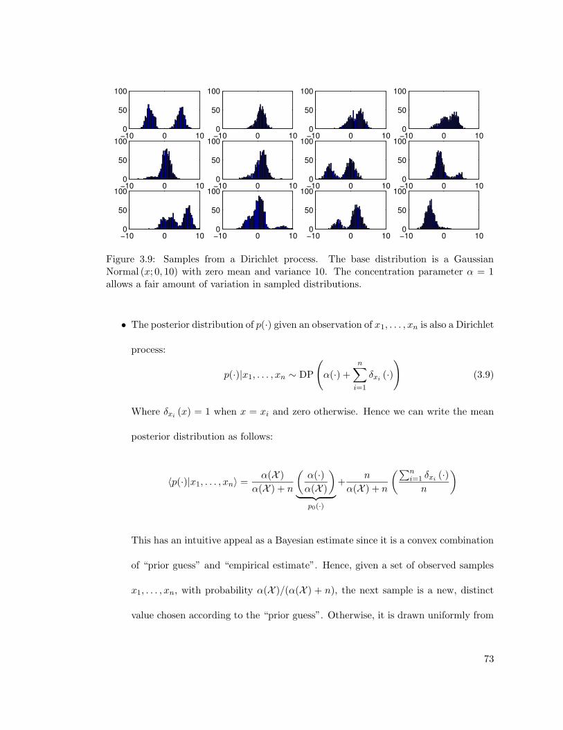
−10 0 100

50

100

−10 0 100

50

100

−10 0 100

50

100

−10 0 100

50

100

−10 0 100

50

100

−10 0 100

50

100

−10 0 100

50

100

−10 0 100

50

100

−10 0 100

50

100

−10 0 100

50

100

−10 0 100

50

100

−10 0 100

50

100

Figure 3.9: Samples from a Dirichlet process. The base distribution is a GaussianNormal (x; 0, 10) with zero mean and variance 10. The concentration parameter α = 1allows a fair amount of variation in sampled distributions.

• The posterior distribution of p(·) given an observation of x1, . . . , xn is also a Dirichlet

process:

p(·)|x1, . . . , xn ∼ DP

(α(·) +

n∑

i=1

δxi (·))

(3.9)

Where δxi (x) = 1 when x = xi and zero otherwise. Hence we can write the mean

posterior distribution as follows:

〈p(·)|x1, . . . , xn〉 =α(X )

α(X ) + n

(α(·)α(X )

)

︸ ︷︷ ︸p0(·)

+n

α(X ) + n

(∑ni=1 δxi (·)n

)

This has an intuitive appeal as a Bayesian estimate since it is a convex combination

of “prior guess” and “empirical estimate”. Hence, given a set of observed samples

x1, . . . , xn, with probability α(X )/(α(X ) + n), the next sample is a new, distinct

value chosen according to the “prior guess”. Otherwise, it is drawn uniformly from

73

among the first n samples. The applicability of the term “concentration parameter”

to α0 is apparant here, since for large values of α0, the sampled distributions will

tend to be very similar to the base distribution, while smaller values of α0 allow

more variation. Figure 3.9 shows sample distributions from a Dirichlet process with

a relatively low concentration parameter α0 = 1 which allows a fair amount of

deviation from the base distribution p0(x) = Normal (x; 0, 10).

• The probability of a new observation xn+1 can be derived from the corresponding

result for Dirichlet distributions by taking the limit as αj → 0 and k → ∞ such

that α(X ) is constant.

p(xn+1 = xi for some 1 ≤ i ≤ n|x1, . . . , xn, α) =

∑ni=1 δxi (xn+1)

α(X ) + n

p(xn+1 6= xi for all 1 ≤ i ≤ n|x1, . . . , xn, α) =α(X )

α(X ) + n

(3.10)

The tractability of equation (3.10) is crucial for sampling methods used to solve DP

models.

Any realization of a Dirichlet process is (with probability 1) a discrete distribution

(Blackwell 1973), since there is always a non-infinitesimal probability of observing a

sample that we have seen before. In this sense, the Dirichlet process can be thought of as

an infinite-dimensional extension of the standard Dirichlet distribution, and its connection

to the Polya urn representation is also well documented (Blackwell & MacQueen 1973,

Chun et al. 2003, Ghosh & Ramamoorthi 2003). While the discreteness of the Dirichlet

process might seem to curb its applicability to modeling continuous distributions, this

74

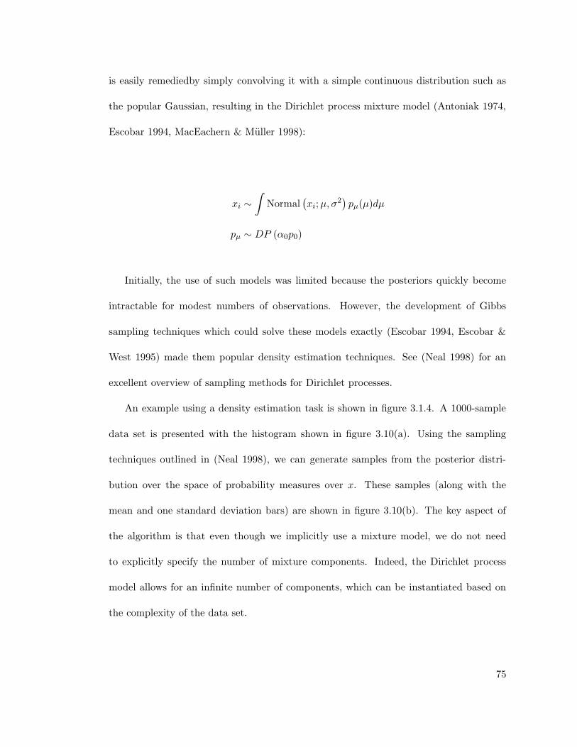
is easily remediedby simply convolving it with a simple continuous distribution such as

the popular Gaussian, resulting in the Dirichlet process mixture model (Antoniak 1974,

Escobar 1994, MacEachern & Muller 1998):

xi ∼∫

Normal(xi;µ, σ

2)pµ(µ)dµ

pµ ∼ DP (α0p0)

Initially, the use of such models was limited because the posteriors quickly become

intractable for modest numbers of observations. However, the development of Gibbs

sampling techniques which could solve these models exactly (Escobar 1994, Escobar &

West 1995) made them popular density estimation techniques. See (Neal 1998) for an

excellent overview of sampling methods for Dirichlet processes.

An example using a density estimation task is shown in figure 3.1.4. A 1000-sample

data set is presented with the histogram shown in figure 3.10(a). Using the sampling

techniques outlined in (Neal 1998), we can generate samples from the posterior distri-

bution over the space of probability measures over x. These samples (along with the

mean and one standard deviation bars) are shown in figure 3.10(b). The key aspect of

the algorithm is that even though we implicitly use a mixture model, we do not need

to explicitly specify the number of mixture components. Indeed, the Dirichlet process

model allows for an infinite number of components, which can be instantiated based on

the complexity of the data set.

75

−8 −6 −4 −2 0 2 4 6 8 100

5

10

15

20

25

30

35

40

45

50

(a) Histogram of 1000 samples of data.

−8 −6 −4 −2 0 2 4 6 8 100

0.05

0.1

0.15

0.2

0.25

(b) Samples from the estimated distribution.

Figure 3.10: The right sub-figure shows samples from the posterior distribution overprobability densities (light grey lines), estimated from the data on the left using a Dirichletprocess prior. Also shown are the mean (thick dark line) and standard deviation (thickdashed lines) of the sampled distributions.

An alternate set of sampling methods using the stick-breaking construction of the

Dirichlet process by Sethuraman (1994) has also gained in popularity, leading to the trun-

cated versions of the Dirichlet process (Ishwaran & James 2001, Ishwaran & Zarepour

2002). Variational methods for the Dirichlet process which use this truncated represen-

tation also exist (Blei & Jordan 2004), although algorithmically, they reduce again to

the existing methods proposed in (Beal 2003) which initially overestimate the number of

components, and then allow the inference mechanism to prune away the unneeded model

complexity.

Some of our recent efforts have been directed towards examining whether locally

weighted projection regression (LWPR) (Vijayakumar et al. 2000), an extremely efficient

supervised learning algorithm based on the creation of fixed local models, can be inter-

preted in the framework of Dirichlet process mixtures.

76

The key similarity is the generation of new local models. As Neal (1998) intuitively

describes, in the Gibbs sampling algorithm, a data point has a higher probability of

spawning a new Dirichlet process mixture component if it cannot be explained satisfac-

torily by existing components. This is exactly the same heuristic that is used by LWPR

for the creation of new local models.

At this time the Dirichlet process model is still computationally unattractive due to

the Gibbs sampling procedure which limits its applicability to higher-dimensional param-

eter spaces. Although it has been used with limited success in some supervised learning

settings (Rasmussen 2000, Rasmussen & Ghahramani 2002, Beal et al. 2002), the varia-

tional approach of Blei & Jordan (2004) and our growing mixture formulation presented

in this section seem more promising and empirically seem to require fewer iterations to

converge.

3.2 Online Learning with Automatic Forgetting Rates

While there exists a large body of statistical learning literature that deals with Bayesian

techniques for batch learning, many of these techniques are not naturally applicable to

sequential learning tasks that are often embedded in dynamic, non-stationary environ-

ments. Two aspects of online learning make statistical learning especially hard. Firstly,

the parameters of interest (e.g. the parameters of a classification/regression function)

may themselves vary with time. In addition, a complex learning algorithm with multiple

parameters in flux, may cache statistics based on only partially converged estimates of

these parameters. It therefore becomes necessary to “forget” past data and statistics,

77

in favor of more recent observations, such that the learning system is responsive to new

conditions at an appreciable rate, as the learning model and environment evolve.

In the context of regression, the popular Recursive Least Squares (RLS) algorithm

(Ljung & Soderstrom 1983) has received considerable attention. Crucial to this framework

is the notion of a “forgetting rate” γ (where 0 ≤ γ ≤ 1), which controls the extent to

which past data contributes towards the current estimate of the process parameters. In

a sense, the forgetting rate γ can be thought of as defining an effective window of size

γ/(1 − γ) over the data. Several algorithms adapt this strategy to limit the horizon

of accumulated “sufficient statistics”, including the recent model estimation framework

using variational Bayes (Sato 2001).

Recently, an alternative view within the framework of Bayes filtering has been pro-

posed (de Freitas et al. 1999, Sykacek & Roberts 2003). This framework treats the

estimation of the parameters of a non-stationary process as a Bayesian state estima-

tion problem. Several algorithms exist for performing state estimation including the

well-known Kalman filter. Indeed, statistical signal processing literature often highlights

the relationship between RLS based system identification, and Kalman filters (Proakis

et al. 2002). In (Sykacek & Roberts 2003), an algorithm for online classification is pre-

sented that uses the variational Bayes framework in conjunction with a Kalman filter, to

automatically estimate the process noise variance — a crucial parameter in determining

the extent of non-stationarity. The algorithm however, only considers causal informa-

tion flow (Kalman filtering), even though a windowing approach is used which could

potentially take advantage of anti-causal information flow (Kalman smoothing) as well.

78

3.2.1 Using a Kalman Filter to Track Non-Stationarity

A simple way of dealing with a non-stationary parameter, is to formulate it as a “drifting”

random variable (Sykacek & Roberts 2003), and track it with a Bayes filter. For the

purposes of this exposition, let us consider a simple regression problem, in which each

data point (yn|xn) is generated according to the following model:

wn = wn−1 + ηn (3.11)

yn = wnxn + εn (3.12)

where ηn and εn are additive Gaussian noise distributed as ηn ∼ Normal (ηn; 0, 1/λ)

and εn ∼ Normal (εn; 0, 1/ψy). Note the subscript n for the regression coefficient w

indicates that we treat it as a drifting parameter whose value changes with time according

to equation (3.11). Since these equations represent a linear, Gaussian state-space model,

a Bayes filter reduces to the well known Kalman filter (Kalman 1960).

Knowledge of the precision λ is crucial if we wish to track wn accurately, since it

constrains the amount that wn is allowed to vary at each time step. As shown in figure

3.11, an incorrect estimate of λ can result in a learning system that is too sluggish to

adapt to changes (if λ is too high), or one that is excessively responsive, and highly

susceptible to noise (if λ is too low). Thus λ can be interpreted as an inverse process

adaptation rate, or perhaps more accurately, an inverse drift step size. Estimating λ (and

also ψy) is potentially achievable if we retain a moving window of N data points (we

shall revisit the question of window size later) in conjunction with a Kalman smoothing

79

100 200 300 400 500 600 700 800 9005

5.2

5.4

5.6

5.8

6

6.2

6.4

6.6

time

w

true whigh λlow λ

Figure 3.11: Overestimating the precision λ results in sluggish tracking of rapid changesin w, while underestimating it introduces a hyper-sensitivity to noise.

procedure to estimate true posteriors over the wn within the window. Clearly, a naive

Maximum-Likelihood (ML) estimation of both λ and ψy simultaneously, is impossible

without arriving at degenerate Gaussian distributions over wn. This is partially because

λ and ψy are essentially model complexity parameters, since they restrict the possible

space of Markov chains of wn given a starting distribution p(w0). Consequently, they also

restrict the possible space of data sets that could be observed under this model structure.

Hence, we look towards the evidence framework to provide the necessary regularization

ability such that we can obtain principled estimates of these quantities from the point of

view of maximizing model evidence.

We therefore place prior distributions over λ and ψy. Since they are essentially scale

parameters, we choose the prior distributions to be broad (non-informative) Gamma

distributions, which are theoretically justified as being relatively uniform over a log scale

(Gelman et al. 1995), as well as analytically convenient due to their conjugacy with

Normal distributions:

80

λ

w0

ζ0

y1 y2 y3 yN

wNw1 w2 w3w0

ψy

x2x1 x3 xN

bψaψ

aλ bλ

Figure 3.12: Graphical model for variational Kalman filtering

λ ∼ Gamma (λ; aλ, bλ) =baλλ

Γ (aλ)λaλ−1 exp (−bλλ) (3.13)

ψy ∼ Gamma (ψy; aψ, bψ) =baψψ

Γ (aψ)ψaψ−1y exp (−bψψy) (3.14)

The graphical model incorporating these distributions is shown in figure 3.12. Given

the conditional independencies implied by this model, the log complete evidence can be

written as follows:

81

ln p(y,w, λ, ψy|x) =

N∑

n=1

[1

2lnψy2π− ψy

2(yn − wnxn)2

+1

2ln

λ

2π− λ

2(wn − wn−1)2

]

+1

2lnζ0

2π− ζ0

2(w0 − w0)2

+ aλ ln bλ − ln Γ (aλ) + (aλ − 1) lnλ− bλλ

+ aψ ln bψ − ln Γ (aψ) + (aψ − 1) lnψy − bψψy

(3.15)

where we define y =

[y1 · · · yN

]T, x =

[x1 · · · xN

]T, w =

[w1 · · · wN

]T.

Ultimately, we are interested in the posterior distribution over the regression coefficient

at the current (last) time step, i.e. p(wN |xDN ), which is obtained by marginalizing out all

the other random variables from the true posterior p(w, λ, ψy|xDN ). From the structure

of equation (3.15), we see that this is an analytically intractable proposition. We therefore

turn to the factorial variational approximation methods described in chapter 2 to allow

tractable inference of the model parameters.We shall choose to approximate the true

posterior p(w, λ, ψy|xDN ) with the factored approximating ensemble:

Q(w, λ, ψy) = Q(w)Q(λ, ψy) (3.16)

The factorization between Q(w) and Q(λ, ψy) is the approximation we introduce to

allow tractable inference. As it turns out, an additional factorization Q(λ)Q(ψy) falls out

of the conditional independencies in the model itself (the graph vertices corresponding to

λ and ψy are separated by w).

82

Inference of the individual posterior distributions proceeds by iteratively updating

each Qi(·) in equation (3.16) according to equation (2.6). Given the factorization in

equation (3.16), estimating the posterior distribution Q(w) over the regression coefficients

is equivalent to performing the forward (filtering) and backward (smoothing) recursions

of a Kalman smoother, given current estimates of Q(λ) and Q(ψy). If we assume that the

filtered distribution of wn is Q(wn|xD1:n) = Normal (wn; 〈wn〉n , 1/ζn), and the smoothed

distribution isQ(wn|xD1:N) = Normal (wn; 〈wn〉N , 1/ϕn), then we can derive the following

forward recursion:

ζn = 〈ψy〉x2n +

ζn−1 〈λ〉ζn−1 + 〈λ〉

〈wn〉n =1

ζn

[〈ψy〉xnyn +

〈λ〉 ζn−1 〈wn−1〉n−1

ζn−1 + 〈λ〉

]

as well as the backward recursion:

ϕn−1 =ϕn(ζn−1 + 〈λ〉

)2

ϕn(ζn−1 + 〈λ〉

)+ 〈λ〉2

〈wn−1〉N =ϕnϕn−1

[(ζn−1 〈wn−1〉n−1 + 〈λ〉 〈wn〉N

)(ζn−1 + 〈λ〉

)

ϕn(ζn−1 + 〈λ〉

)+ 〈λ〉2

]

The update equations for the distributions of Q(λ) and Q(ψy) are easily derived as

Gamma distributions from equations (3.15) and (2.6). This results in the following update

equations (see appendix B.3) for the parameters of the posterior Gamma marginals Q(λ)

and Q(ψy):

83

200 400 600 800 10005

5.5

6

6.5

w

(a) True (drifting) w

200 400 600 800 1000

102

104

λ

vkS estimatevkF estimate

(b) Estimating λ

Figure 3.13: In our artificial data set, the regression parameter drifts as shown in 3.13(a).The estimates of λ obtained by the vkS and vkF algorithms (for ψy = 104) are shown in3.13(b)

aψ = aψ +N

2

bψ = bψ +1

2

N∑

n=1

[(yn − 〈wn〉N xn

)2+

1

ϕn

]

aλ = aλ +N

2

bλ = bλ +1

2

N∑

n=1

[(〈wn〉N − 〈wn−1〉N

)2+

1

ϕn+

1

ϕn−1− 2 Cov (wn−1, wn)

]

where Cov (wn−1, wn) is the cross-time covariance that can be derived using Schur com-

plements (see appendix A.1) as:

Cov(wn−1, wn) =〈λ〉(ζn−1 + 〈λ〉

)

ϕn−1

[ϕn(ζn−1 + 〈λ〉

)+ 〈λ〉2

]

84

3.2.2 Bayesian Forgetting Rates Evaluation

To evaluate our algorithm we considered the simple linear regression system outlined in

section 3.2.1. We allow w to drift over 1000 time steps according to the plot in figure

3.13(a). At each time step we sample xn according to Normal (xn; 0, 1), a zero mean, unit

variance Gaussian, and generate yn according to equation (3.12). We generate 50 such

data sets in each of three categories, corresponding to the observation noise precision set

at ψy = 102, ψy = 103, and ψy = 104, for a total of 150 data sets.

We evaluated our variational Kalman smoother (vkS) algorithm against two others

on the generated data sets: the variational Kalman filter (vkF) algorithm of (Sykacek

& Roberts 2003) (adapted for regression instead of classification), and RLS. In order to

select the optimum value for the window size parameter N in vkF, it was evaluated at

several values ranging from 10 to 200 time steps, and the window size giving the smallest

mean-squared error with the true w was chosen. In a similar manner the forgetting rate

γ for RLS was chosen using a line search to minimize the mean-squared error between

the estimated and the true w.

Note that our vkS algorithm did not have access to the true w, but as figure 3.14

shows, it performs the best of the 3 algorithms across all noise ranges. As the results show,

the vkS algorithm tends to outperform RLS significantly. The vkF algorithm performs

comparably at estimating w, but as figure 3.13(b) shows, it tends to underestimate λ

due to the lack of anti-causal information that is useful in smoothing out past estimates.

Underestimating λ causes it to be slightly more susceptible to output noise than our vkS

method.

85

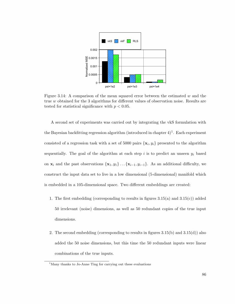
Figure 3.14: A comparison of the mean squared error between the estimated w and thetrue w obtained for the 3 algorithms for different values of observation noise. Results aretested for statistical significance with p < 0.05.

A second set of experiments was carried out by integrating the vkS formulation with

the Bayesian backfitting regression algorithm (introduced in chapter 4)1. Each experiment

consisted of a regression task with a set of 5000 pairs xi, yi presented to the algorithm

sequentially. The goal of the algorithm at each step i is to predict an unseen yi based

on xi and the past observations x1, y1 . . . xi−1, yi−1. As an additional difficulty, we

construct the input data set to live in a low dimensional (5-dimensional) manifold which

is embedded in a 105-dimensional space. Two different embeddings are created:

1. The first embedding (corresponding to results in figures 3.15(a) and 3.15(c)) added

50 irrelevant (noise) dimensions, as well as 50 redundant copies of the true input

dimensions.

2. The second embedding (corresponding to results in figures 3.15(b) and 3.15(d)) also

added the 50 noise dimensions, but this time the 50 redundant inputs were linear

combinations of the true inputs.

1Many thanks to Jo-Anne Ting for carrying out these evaluations

86

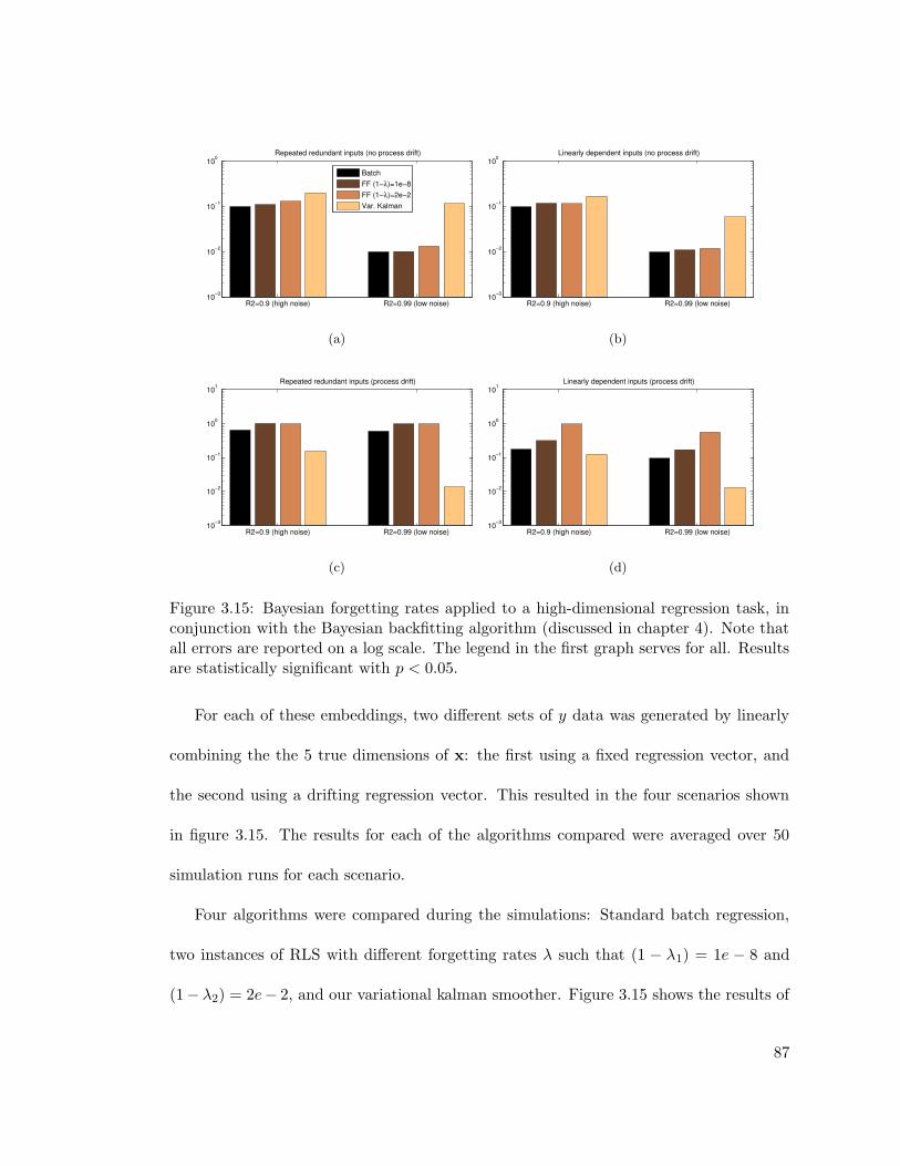
R2=0.9 (high noise) R2=0.99 (low noise)10−3

10−2

10−1

100Repeated redundant inputs (no process drift)

BatchFF (1−λ)=1e−8FF (1−λ)=2e−2Var. Kalman

(a)

R2=0.9 (high noise) R2=0.99 (low noise)10−3

10−2

10−1

100Linearly dependent inputs (no process drift)

(b)

R2=0.9 (high noise) R2=0.99 (low noise)10−3

10−2

10−1

100

101Repeated redundant inputs (process drift)

(c)

R2=0.9 (high noise) R2=0.99 (low noise)10−3

10−2

10−1

100

101Linearly dependent inputs (process drift)

(d)

Figure 3.15: Bayesian forgetting rates applied to a high-dimensional regression task, inconjunction with the Bayesian backfitting algorithm (discussed in chapter 4). Note thatall errors are reported on a log scale. The legend in the first graph serves for all. Resultsare statistically significant with p < 0.05.

For each of these embeddings, two different sets of y data was generated by linearly

combining the the 5 true dimensions of x: the first using a fixed regression vector, and

the second using a drifting regression vector. This resulted in the four scenarios shown

in figure 3.15. The results for each of the algorithms compared were averaged over 50

simulation runs for each scenario.

Four algorithms were compared during the simulations: Standard batch regression,

two instances of RLS with different forgetting rates λ such that (1 − λ1) = 1e − 8 and

(1− λ2) = 2e− 2, and our variational kalman smoother. Figure 3.15 shows the results of

87

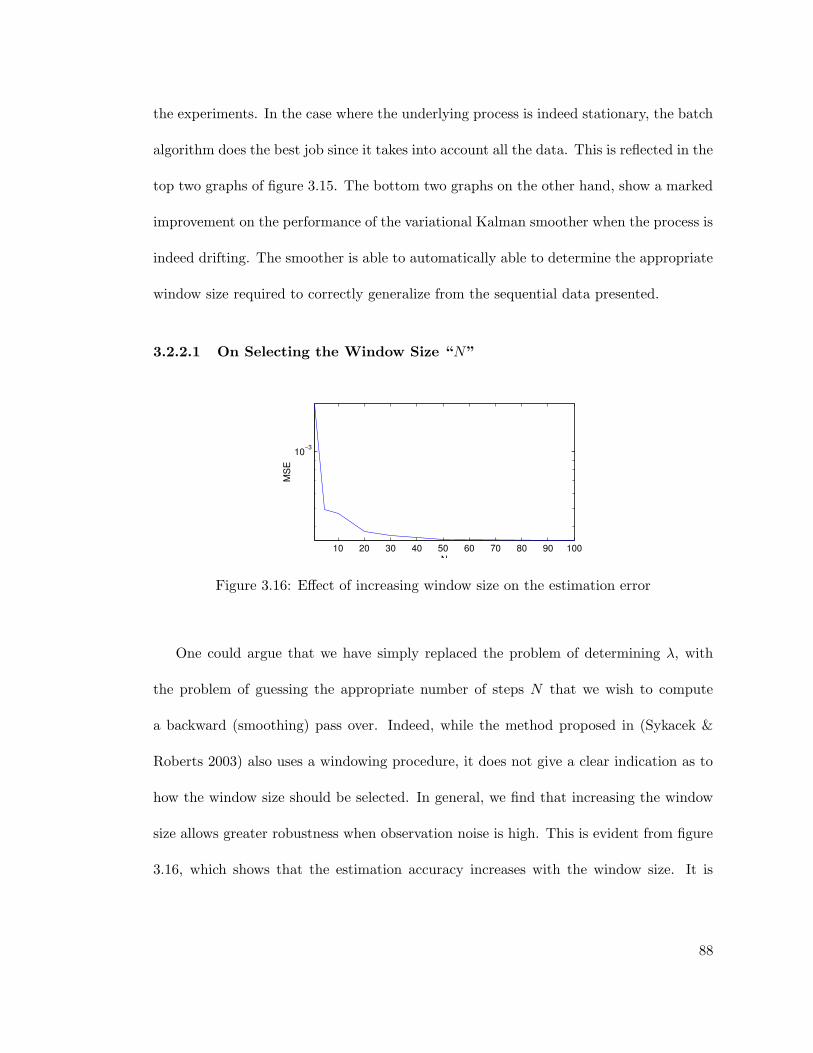
the experiments. In the case where the underlying process is indeed stationary, the batch

algorithm does the best job since it takes into account all the data. This is reflected in the

top two graphs of figure 3.15. The bottom two graphs on the other hand, show a marked

improvement on the performance of the variational Kalman smoother when the process is

indeed drifting. The smoother is able to automatically able to determine the appropriate

window size required to correctly generalize from the sequential data presented.

3.2.2.1 On Selecting the Window Size “N”

10 20 30 40 50 60 70 80 90 100

10−3

N

MS

E

Figure 3.16: Effect of increasing window size on the estimation error

One could argue that we have simply replaced the problem of determining λ, with

the problem of guessing the appropriate number of steps N that we wish to compute

a backward (smoothing) pass over. Indeed, while the method proposed in (Sykacek &

Roberts 2003) also uses a windowing procedure, it does not give a clear indication as to

how the window size should be selected. In general, we find that increasing the window

size allows greater robustness when observation noise is high. This is evident from figure

3.16, which shows that the estimation accuracy increases with the window size. It is

88

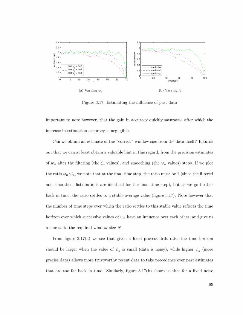
0 10 20 30 40 50 60 701

1.2

1.4

1.6

1.8

2

2.2

2.4

iterations

varia

nce

ratio

true ψy = 1e2

true ψy = 1e3

true ψy = 1e4

(a) Varying ψy

0 20 40 60 80 1001

1.2

1.4

1.6

1.8

2

2.2

timesteps

varia

nce

ratio

true λ=1e4true λ=1e3true λ=1e2

(b) Varying λ

Figure 3.17: Estimating the influence of past data

important to note however, that the gain in accuracy quickly saturates, after which the

increase in estimation accuracy is negligible.

Can we obtain an estimate of the “correct” window size from the data itself? It turns

out that we can at least obtain a valuable hint in this regard, from the precision estimates

of wn after the filtering (the ζn values), and smoothing (the ϕn values) steps. If we plot

the ratio ϕn/ζn, we note that at the final time step, the ratio must be 1 (since the filtered

and smoothed distributions are identical for the final time step), but as we go further

back in time, the ratio settles to a stable average value (figure 3.17). Note however that

the number of time steps over which the ratio settles to this stable value reflects the time

horizon over which successive values of wn have an influence over each other, and give us

a clue as to the required window size N .

From figure 3.17(a) we see that given a fixed process drift rate, the time horizon

should be larger when the value of ψy is small (data is noisy), while higher ψy (more

precise data) allows more trustworthy recent data to take precedence over past estimates

that are too far back in time. Similarly, figure 3.17(b) shows us that for a fixed noise

89

level in the output, a higher value of λ (slowly changing process) tends to stretch the

window, while a lower value of λ (rapidly changing process) tends to require a smaller

window. Our evaluations of vkS in the previous section monitor this quantity to ensure

an appropriately large window size.

Thus we essentially have a parameter-free algorithm that is able to automatically

determine its own adaptation rate within a principled framework.

3.3 Bayesian Supersmoothing

Kernel-based methods have been highly popular in statistical learning, starting with

Parzen windows, kernel regression, locally weighted regression, radial basis function net-

works, and more recently in formulations involving RKHS such as support vector ma-

chines, and Gaussian process regression. In general, most algorithms start out with

kernel parameterizations that are the same for all kernels, independent of where in the

data space the kernel is used, but later recognize the advantage of locally adaptive ker-

nels, e.g. (Friedman 1984, Poggio & Girosi 1990, Schaal & Atkeson 1998, Paciorek &

Schervish 2004). This progression of algorithms is motivated by a large class of learn-

ing problems in which the properties of learning data vary strongly throughout the data

space, for instance, as in regression problems with different frequency characteristics in

different parts of the work space, or, as phrased in Gaussian process regression, with

non-stationary covariance functions. However, while optimization of the parameters of

one globally shared kernel is already quite expensive for most algorithms — e.g., it con-

stitutes the bulk of the computation in Gaussian process regression (Williams 1997) —

90

performing such optimization for every kernel individually becomes rather complex and

prone to overfitting due to the flood of open parameters. It thus seems natural to seek a

completely Bayesian treatment of local kernel adaptation, i.e., to integrate out complexity

parameters, ideally with an EM-like algorithm such that gradient descent and sampling

problems can be avoided.

For non-parametric locally weighted regression (Atkeson, Moore & Schaal 1997), we

assume a training set xD = xi, yiNi=1 drawn from a nonlinear function y = f(x) + ε

contaminated by mean-zero noise ε. We wish to approximate a locally linear model

β =

[β1 β0

]Tof this function, i.e., the slope and intercept of the tangent at a query

point xq, and subsequently make a prediction yq =

[xq 1

]β. For this purpose, we

assume the existence of a spatially localized weighting kernel wi = k(xi, xq, h) that assigns

a weight to every training point according to its Euclidean distance from the query point.

The Gaussian RBF kernel wi = exp(−0.5h (xi − xq)2

)is a popular choice, but as will

be shown below, not always the most convenient formulation. The bandwidth h of the

kernel is a crucial parameter that determines the quality of fit of the locally linear model.

If h is too large, we may overfit the data, and if it is too small, we may oversmooth.

In general, h needs to be chosen as a function of the local curvature of f(x) and the

data density around the query point. If we can find a good bandwidth as a function of

xq, nonlinear function approximation can be solved accurately and efficiently. Our goal

is to find a Bayesian formulation of determining β and h simultaneously in an EM-like

algorithm.

91

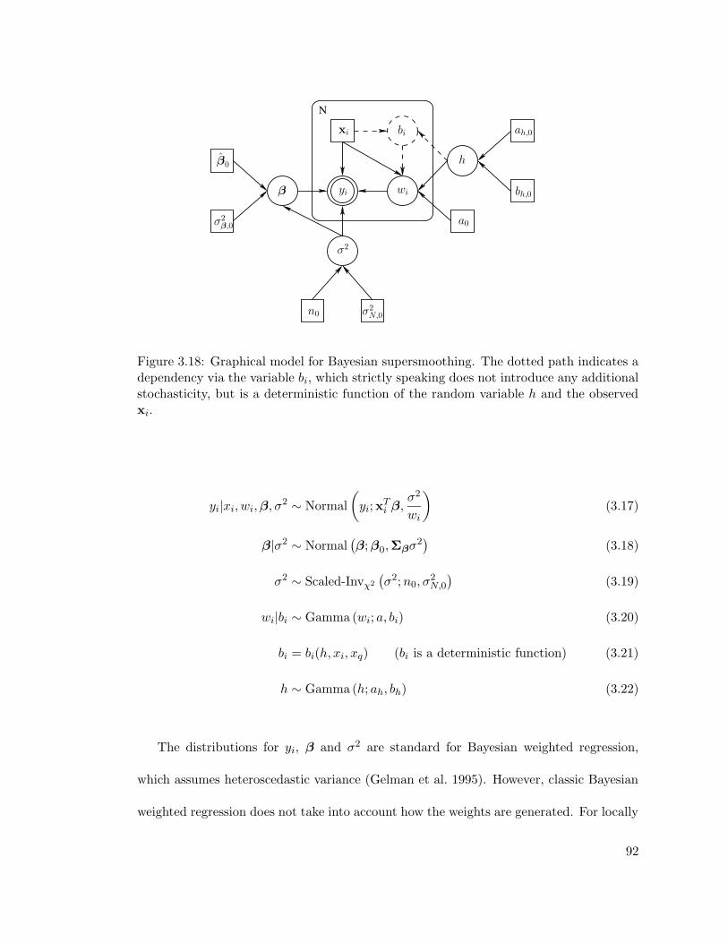
N

h

β

bi

n0 σ2N,0

σ2

β0

σ2β,0

wiyi

a0

bh,0

ah,0xi

Figure 3.18: Graphical model for Bayesian supersmoothing. The dotted path indicates adependency via the variable bi, which strictly speaking does not introduce any additionalstochasticity, but is a deterministic function of the random variable h and the observedxi.

yi|xi, wi,β, σ2 ∼ Normal

(yi; x

Ti β,

σ2

wi

)(3.17)

β|σ2 ∼ Normal(β;β0,Σβσ

2)

(3.18)

σ2 ∼ Scaled-Invχ2

(σ2;n0, σ

2N,0

)(3.19)

wi|bi ∼ Gamma (wi; a, bi) (3.20)

bi = bi(h, xi, xq) (bi is a deterministic function) (3.21)

h ∼ Gamma (h; ah, bh) (3.22)

The distributions for yi, β and σ2 are standard for Bayesian weighted regression,

which assumes heteroscedastic variance (Gelman et al. 1995). However, classic Bayesian

weighted regression does not take into account how the weights are generated. For locally

92

weighted regression, heteroscedastic variance is modeled as an effect of the weighting

kernel, i.e., as growing noise variance proportional to the distance of a data point away

from the query point. In order to obtain a probabilistic formulation, we introduce a

conditional Gamma distribution over each weight:

p(wi|h) =[bi (xi, xq, h)]a0

Γ (a0)wa0i exp (−wibi (xi, xq, h))

bi (xi, xq, h) =1

k (xi, xq, h)

which implies:

〈wi〉 =a0

bi (xi, xq, h)= a0k (xi, xq, h)

Var (wi) = a0k (xi, xq, h)2

(3.23)

There are some important observations concerning equation (3.23). The expectation

of a weight is just the weighting kernel k scaled by a0. This scaling is harmless in weighted

regression since a uniform scaling of all weights does not affect the estimation of the locally

linear model. The variance of the weights however, is proportional to the squared value

of the kernel k. Thus data points with a tiny weight will have an even tinier variance,

while data points with larger weights will have more variance. This nonlinear dependence

of the variance on the distance from the query point is quite useful: at a point very far

away from the query point, the kernel value is close to zero, and we should rightfully be

confident that this point is irrelevant to the local regression. However data that receive

a significant activation of the kernel k should be scrutinized carefully.

93

3.3.1 An EM-Like Learning Algorithm

In order to derive a learning algorithm for the graphical model of figure 3.18, we shall

employ the factorial variational approximation discussed in chapter 2. The log joint

distribution over the variables in the graphical model can be written as:

ln p(xD,xH;φ) = −N2

lnσ2 +N∑

i=1

[1

2lnwi −

wi2σ2

(yi − βTxi

)2]

+N∑

i=1

[a0 ln bi (xi, xq, h) + (a0 − 1) lnwi − wibi (xi, xq, h)

]

− 1

2ln |Σβ,0| −

1

2lnσ2 − 1

2σ2

(β − β0

)TΣ−1β,0

(β − β0

)

−(n0

2+ 1)

lnσ2 −nσ2

N,0

2σ2+ (ah,0 − 1) lnh− bh,0h+ constxD,xH

Our factorial variational approximation for this model is of the form:

Q(xH) = Q(β, σ2)Q(h)N∏

i=1

Q(wi) (3.24)

Using the formula for the updates of the distributions under the factorial assump-

tion in equation 2.6, we can derive the following updates for the distributions over the

regression parameters:

Σβ =

(N∑

i=1

〈wi〉xixTi + Σ−1β,0

)−1

β = Σβ

(N∑

i=1

〈wi〉 yixi + Σ−1β,0β0

) (3.25)

94

and the noise variance:

σ2N =

∑Ni=1 〈wi〉

(yi − β

Txi

)2+(β − β0

)TΣ−1β,0

(β − β0

)+ n0σ

2N,0

n0 +N

n = n0 +N

(3.26)

Even more interesting is the posterior distribution over the weights wi which becomes:

a = a0 +1

2

bi =1

2σ2N

(yi − β

Txi

)2+

1

2xiTΣβxi + 〈bi (xi, xq, h)〉

〈wi〉 =a

bi=

a0 + 12

12σ2N

(yi − β

Txi

)2+ 1

2xiTΣβxi + 〈bi (xi, xq, h)〉

(3.27)

And finally, the log posterior of the bandwidth h can be written as:

lnQ(h) = a0

N∑

i=1

ln bi (xi, xq, h)−N∑

i=1

〈wi〉 bi (xi, xq, h) + (ah,0 − 1) lnh− bh,0h+ consth

(3.28)

As an obvious problem, equation (3.28) does not have a compatible form for a log-

Gamma distribution in h when using the general formulation bi = 1/k (xi, xq, h). We

therefore have to investigate concrete formulations of weighting kernels. In particular we

consider the following popular choices, (Atkeson et al. 1997):

k = exp

(−1

2h (xi − xq)2

)(3.29)

95

k = (1 + h (xi − xq)p)−1 (3.30)

k =

(1− h (xi − xq)2

)pif h (xi − xq)2 ≤ 1

0 otherwise

(3.31)

Where p is a positive even integer. In order to be conjugate with the Gamma dis-

tribution in h, we can only accept terms in equation (3.28) that are linear or log-linear

in h. None of the kernels in (3.29)–(3.31) fulfills this requirement. Indeed, only a kernel

that is linear in h would ever result in linear and log-linear terms. Unfortunately, such

a kernel is ineffective for bandwidth adaptation in weighted regression, as the bandwidth

would just act as a scale parameter on all weights. By inspecting equation (3.25) under

the assumption of uninformative priors, it becomes apparent that such a scaling would

have no effect on estimating the local linear model’s regression parameters β. Therefore,

in order to find an analytical update for the posterior distribution of h, we will thus

have to resort to further approximations. For our kernels in (3.29)–(3.31), the potentially

problematic terms in equation (3.28) are respectively:

N∑

i=1

[1

2a0h (xi − xq)2 − 〈wi〉 exp

(1

2(xi − xq)2

)](3.32)

N∑

i=1

[a0 ln

(1 + h (xi − xq)p

)− 〈wi〉

(1 + h (xi − xq)p

)](3.33)

N∑

i=1

[−a0p ln

(1− h (xi − xq)2

)− 〈wi〉

(1− h (xi − xq)2

)−p](3.34)

96

While equation (3.34) has no linear or log-linear terms in h, both equations (3.32)

and (3.33) seem more promising, as the terms involve only concave/convex nonlinearities,

which can be easily approximated by a bound. However, equation (3.32) has a subtle

additional problem: the sign on the first summand is positive, while in a log-Gamma

distribution, the terms linear in h should be negative. This could potentially lead to

negative parameters in the posterior which are a result of the approximating process

(which indeed occurs when realizing the algorithm with a Gaussian kernel). We therefore

proceed with the kernel corresponding to equation (3.33), and with some foresight towards

the final algorithm, we choose the following more general parameterization:

k(xi, xq, h) =1

bi (xi, xq, h)where bi = s

(1 + h (xi − xq)p

)(3.35)

Using the variational approach suggested by Jaakkola & Jordan (2000), we can bound

the problematic first term in equation (3.33) as:

ln(

1 + h (xi − xq)p)≥ λi ln

(h (xi − xq)p

)− λi

λi1− λi

+ ln

(1

1− λi

)

where the λi are the variables that parameterize a family of lower bounds, and which

must be individually optimized to ensure a tight bound. With this approximation, equa-

tion (3.28) simplifies, and the following updates to the posterior distribution over h can

be derived:

97

lnQ(h) = a0

N∑

i=1

λi lnh− sN∑

i=1

〈wi〉h (xi − xq)p + (ah,0 − 1) lnh− bh,0h

ah = ah,0 + a0

N∑

i=1

λi

bh = sN∑

i=1

〈wi〉 (xi − xq)p + bh,0

(3.36)

Finally, the variational parameters λi need to be optimized. Fortunately, this opti-

mization decomposes into decoupled optimizations for each λi of the form:

∂

∂λi

(λi 〈lnh (xi − xq)p〉 − λi ln

λi1− λi

+ ln

(1

1− λi

))= 0 (3.37)

for which the solution is:

λi =ϕi

1 + ϕiwhere ϕi = (xi − xq)p

1

2ψ (ah)bh

where ψ (·) is the digamma function. We can therefore write the final EM-like procedure

as:

E-Step: Apply equations (3.25), (3.26), (3.27) and (3.36)

M-Step: Apply equation (3.37)

98

3.3.2 Bayesian Supersmoothing Evaluations

We evaluated Bayesian supersmoothing in several synthetic one-dimensional data sets.

In all simulations, we chose the prior parameters to be:

ah,0 = 0.1, bh,0 = 1e− 4, a0 = 10, n0 = 10, σ2N,0 = 0.1, β0 = 0,Σβ,0 = 1e6I

This choice of priors corresponds to a rather uninformative initial bias that h = 1000

and that we believe to have seen n0 = 10 points with variance σ2N,0, prior to fitting

our model. For the regression parameters we have a highly uninformative distribution

(effectively no bias). The particular values selected for initialization were, on one hand,

motivated by providing numerical stability to the algorithm even if there were no points

falling within the range of the locally linear model, and on the other hand, by our desire to

start out with a moderately small weighting kernel. For weighted regression, there is, in

most cases, a local maximum for the algorithm when performing global linear regression,

and it is this local maximum that we try to avoid in our algorithm.

A more important initialization is the scale s of the weighting kernel in equation (3.35).

On inspection of the posterior distribution over the weights in equation (3.27), one re-

alizes that the weight update is influenced by three terms; the original kernel weight,

the variance of the regression parameters, and the squared standardized residual error of

a data point. The term with the variance of the regression parameters xiTΣβxi is in-

versely proportional to the number of data points contributing to the locally linear model

(c.f. equation (3.25)), and drops quickly to zero for moderate amounts of data. Thus, the

99

denominator of the posterior update of a data point’s weight in equation (3.27) is primar-

ily a tradeoff between the standardized error of the data point and its prior weight. If the

standardized error were to dominate this update, our prior weighting would be ignored

— empirically, we notice that this leads to overfitting. In contrast, if the standardized

error residual were ignored, we will oversmooth. We choose s = 0.01 as a good tradeoff

between residual error and prior kernel weight. Given that both the kernel weight and the

standardized residual error are always in the same range of values, s does not need to be

adjusted or each data set and can be considered to be a one-time model design constant.

In order to have lighter tails on the weighting kernel we choose p = 4 in equation (3.35).

We evaluated Bayesian supersmoothing on three different data sets (see figure 3.19)

and compared it to locally weighted regression (LWR) with a globally optimized Gaussian

weighting kernel using leave-one-out cross validation (Atkeson et al. 1997). The first data

set is generated using the equation:

y(x) = x− sin3(2πx3

)cos(2πx3

)exp

(x4)

with additive i.i.d. noise of 0.1 standard deviation. This function has strongly different

frequency components in different parts of the data space. As figure 3.19(a) shows, LWR

overfits the data in low-frequency areas in order to accommodate the high-frequency

region at the right of the plot. Bayesian supersmoothing correctly adjusts the bandwidth

h with the curvature of the function and does not display any overfitting or underfitting

trends.

100

The very sparse data set in figure 3.19(b) was generated from an initial step function

with a linear trail-off, and a suddenly noisy section of the function. Bayesian supersmooth-

ing properly varies the bandwidth to account for the sudden changes in the function and

the noisy regions. In comparison to LWR, it manages to chisel out the corners of the step

function more accurately while properly smoothing out the noisy regions.

Figure 3.19(c) illustrates that the a high amount of noise in the classic Old Faithful

data set (characterizing the eruption timing of the famous geyser in Yellowstone National

Park), does not mislead Bayesian supersmoothing towards overfitting. The fitting results

are comparable to LWR and the data fits published in (Hastie & Tibshirani 1990).

In general one can conclude that Bayesian supersmoothing adjusts the bandwidth in

all examples over orders of magnitude in order to accommodate the data set at hand. The

lower sub-plot of each example in figure 3.19 illustrates this local bandwidth adaptation

as a function of location in the input space.

While we have focused on seemingly trivial one-dimensional function fitting, we believe

that this is a crucial step towards multi-dimensional settings. As was demonstrated by

D’Souza et al. (2004) with the Bayesian backfitting algorithm (a topic of chapter 4), it is

possible to treat multivariate regression problems in a decomposable fashion by solving

them as a succession of univariate regressions. It is straightforward to combine these two

algorithms into a unified supervised learning framework.

It must be noted however, that our current realization of Bayesian supersmoothing

requires further refinement. As an odd feature of Bayesian weighted regression (Gelman

et al. 1995), equation (3.26) updates σ2N by dividing by n0 +N . Interestingly, this implies

that even a data point which is very far away from the query point (and which therefore

101

should have a very small weight) will have an effect of reducing our posterior variance at

the query point. A variant of the formulation which enforces that∑N

i=1wi = N shows

promise at countering this undesirable behavior.

102

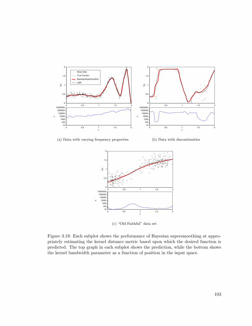
0

0.5

1

1.5

2

0 0.5 1 1.5 2

f(x)

Noisy Data

True Function

BayesianSupersmoother

LWR

10100

100010000

1000001000000

10000000

0 0.5 1 1.5 2

h

x

(a) Data with varying frequency properties

0

0.5

1

1.5

2

0 0.5 1 1.5 2

f(x)

10100

100010000

1000001000000

10000000

0 0.5 1 1.5 2

h

x

(b) Data with discontinuities

0

0.5

1

1.5

2

0 0.5 1 1.5 2

f(x)

10100

100010000

1000001000000

10000000

0 0.5 1 1.5 2

h

x

(c) “Old Faithful” data set

Figure 3.19: Each subplot shows the performance of Bayesian supersmoothing at appro-priately estimating the kernel distance metric based upon which the desired function ispredicted. The top graph in each subplot shows the prediction, while the bottom showsthe kernel bandwidth parameter as a function of position in the input space.

103

Chapter 4

The Quest for Computational Tractability

Real-world data obtained, for instance, from neuroscience, chemometrics, data mining,

or sensor-rich environments, is frequently extremely high-dimensional, severely under-

constrained, and often interspersed with large amounts of irrelevant and/or redundant

features. Combined with the inevitable measurement noise, efficient learning from such

data still poses significant computational challenges to state-of-the-art supervised learn-

ing algorithms, even in linear settings. While traditional supervised learning techniques

such as partial least squares (PLS) regression (Wold 1975), or backfitting (Hastie &

Tibshirani 1990, Hastie & Tibshirani 2000) are often quite efficient and robust for these

problems, they lack a probabilistic interpretation and cannot easily provide analytical

measures of predictive distributions or the evidence of data as needed for model selec-

tion. On the other hand, while recent algorithms in supervised learning compute such

information, they lack computational efficiency as, for instance, in Gaussian process re-

gression or support vector learning.

This chapter presents algorithms that are specifically designed to perform Bayesian

model selection when operating on high-dimensional data in underconstrained situations,

104

Nxd

x2

x1

yi

ψy

b

Figure 4.1: Graphical model for linear regression. Note the fan-in, which causes theestimates of the individual regression coefficients bm to become coupled in the posterior.

while maintaining the computational efficiency and robustness of more traditional statis-

tical techniques. Section 4.1 reviews traditional regression techniques that are designed

to operate on high-dimensional data. In particular, we review the well-known statistical

regression technique of backfitting, and highlight its efficacy as a robust and efficient fam-

ily of supervised learning algorithms. Section 4.2 also reviews some valuable methods for

speeding up statistical computation by structuring data and partial statistics that make

lookup extremely efficient. In section 4.3 we provide a novel probabilistic derivation of

backfitting within the framework of the EM algorithm. This in turn allows us to generalize

this algorithm within the Bayesian framework and perform sophisticated model selection

through the paradigm of evidence maximization. Finally we show that the framework

of sparse Bayesian learning (Tipping 2001) can be derived as a special case of Bayesian

backfitting, and can benefit significantly from its robustness and scalability.

105

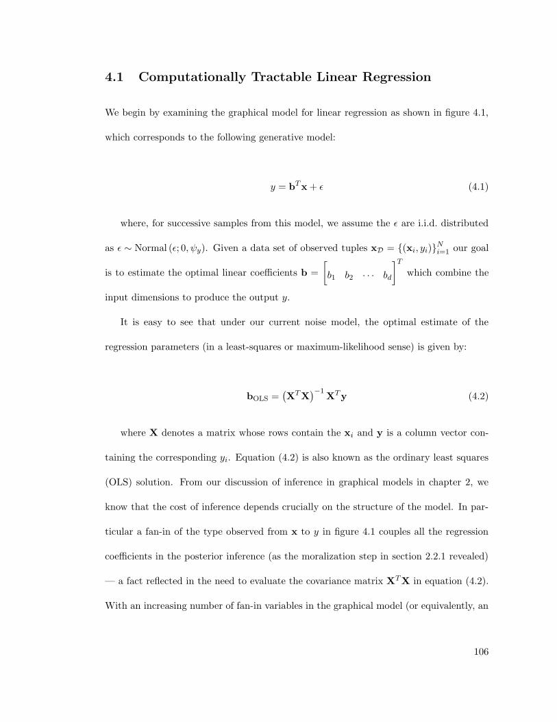
4.1 Computationally Tractable Linear Regression

We begin by examining the graphical model for linear regression as shown in figure 4.1,

which corresponds to the following generative model:

y = bTx + ε (4.1)

where, for successive samples from this model, we assume the ε are i.i.d. distributed

as ε ∼ Normal (ε; 0, ψy). Given a data set of observed tuples xD = (xi, yi)Ni=1 our goal

is to estimate the optimal linear coefficients b =

[b1 b2 · · · bd

]Twhich combine the

input dimensions to produce the output y.

It is easy to see that under our current noise model, the optimal estimate of the

regression parameters (in a least-squares or maximum-likelihood sense) is given by:

bOLS =(XTX

)−1XTy (4.2)

where X denotes a matrix whose rows contain the xi and y is a column vector con-

taining the corresponding yi. Equation (4.2) is also known as the ordinary least squares

(OLS) solution. From our discussion of inference in graphical models in chapter 2, we

know that the cost of inference depends crucially on the structure of the model. In par-

ticular a fan-in of the type observed from x to y in figure 4.1 couples all the regression

coefficients in the posterior inference (as the moralization step in section 2.2.1 revealed)

— a fact reflected in the need to evaluate the covariance matrix XTX in equation (4.2).

With an increasing number of fan-in variables in the graphical model (or equivalently, an

106

increasing input dimensionality d), evaluation of the solution in equation (4.2) becomes

increasingly computationally expensive (approximately O(d3)) and numerically brittle.

While one can attempt to reduce the complexity by efficient matrix inversion techniques

(Belsley, Kuh & Welsch 1980), solutions to this problem typically fall into one of two

categories:

1. Those that try to find a low-dimensional, full-rank representation of the data which

captures the salient information required to perform the regression.

2. Those that deal with the complete dimensionality, but structure computations as ef-

ficiently and robustly as possible (for example, by performing successive inexpensive

univariate regressions).

Sections 4.1.1 and 4.1.2 discuss some of the more popular methods that are represen-

tative of these two classes.

4.1.1 Dimensionality Reduction for Regression

Often the information relevant to predicting the output y can be localized to a low-

dimensional manifold within the domain of x. The methods discussed in this section rely

on the assumption that by performing a dimensionality reduction on the input space, the

resulting lower dimensional manifold captures sufficient information to accurately predict

the output.

107

4.1.1.1 Principal Component Regression

The underlying assumption of principal component regression (PCR) (Massey 1965) is

that the low-dimensional subspace which explains the most variance in the x also cap-

tures the most essential information required to predict y. Starting with the empirical

covariance matrix ΣPCR of the input data:

ΣPCR =1

N − 1

N∑

i=1

xixTi (4.3)

we compute its eigen-decomposition:

ΣPCRvi = λivi (4.4)

where vi is each eigenvector, and λi the corresponding eigenvalue. By projecting

the input x onto the principal K eigenvectors (i.e., the eigenvectors with the largest

eigenvalues) in the columns of the projection matrix U ≡[v1 v2 . . . vK

], we can

compute the regression solution as follows:

bPCR =(UTXTXU

)−1UTXTy (4.5)

Note that as a result of the projection onto the orthogonal eigenvectors v1, . . . ,vK ,

the matrix(UTXTXU

)in equation (4.5) is diagonal, and hence trivial to invert —

the brunt of the computation having already been expended in the eigen-decomposition

step. Hence PCR essentially reduces the multivariate regression to a set of independent

univariate regressions along each of the orthogonal principal component directions.

108

A serious drawback of PCR is that is based purely on variance in the input data

(Schaal, Vijayakumar & Atkeson 1998). The regression solution is therefore highly sen-

sitive to common preprocessing operations such as sphering, which modify the perceived

variance of each input dimension. Hence, low-variance input dimensions which are nev-

ertheless important predictors of the output may be discarded in favor of high-variance,

but irrelevant dimensions. If however, we operate on the joint space z =

[xT y

]Tof

the data we can take the output into consideration when determining the appropriate

lower-dimensional manifold.

4.1.1.2 Joint-Space Factor Analysis for Regression

Factor analysis (FA) (Everitt 1984, Ghahramani & Hinton 1997) is a density estimation

technique which assumes that the observed data z is generated from a lower dimensional

process characterized by K latent or hidden variables v as follows:

zi = Wvi + εi where 1 ≤ i ≤ N (4.6)

If we assume that the latent variables are independently distributed as:

vi ∼ Normal (vi; 0, I)

εi ∼ Normal (εi; 0,Ψ)

109

then the factor loadings W, and the diagonal noise variance matrix Ψ can be easily

estimated using EM (Ghahramani & Hinton 1997), or Bayesian (Ghahramani & Beal

2000) techniques. In joint-space factor analysis for regression (JFR), we define:

z ≡

x

y

and W ≡

Wx

Wy

and Ψ ≡

Ψx 0

0T ψy

(4.7)

Once we estimate W and Ψ for the joint data space of z, we can condition y on x,

and marginalize out the latent variables v to obtain:

〈y|x〉 = Wy

(I + WT

x Ψ−1x Wx

)−1WT

x Ψ−1x︸ ︷︷ ︸

bTJFR

x (4.8)

or equivalently:

bJFR = Ψ−1x Wx

(I + WT

x Ψ−1x Wx

)−1WT

y (4.9)

Note that the required matrix inversion of(I + WT

x Ψ−1x Wx

)is of the order of the la-

tent dimensionality K, which makes this method computationally attractive for problems

in which the underlying latent variable manifold is known to be relatively low dimensional

(i.e. K d).

110

4.1.1.3 Joint-Space Principal Component Regression

Tipping & Bishop (1999) show the relationship between probabilistic versions of factor

analysis and principal component analysis. In particular they show that Factor Anal-

ysis reduces to PCA under the assumption of isotropic output noise (i.e. Ψ = σ2I).

Importantly, they demonstrate that the maximum likelihood solution for W satisfies:

W = U(Λ− σ2I)1/2R (4.10)

where (as before), U is a d × K matrix of principal eigenvectors, Λ is the diagonal

matrix of corresponding eigenvalues, and R is an arbitrary rotation matrix. Given this

result, we can simplify the regression solution for JFR in equation (4.8), and derive the

following joint-space principal component regression (JPCR) solution:

bJPCR = Ux

[I−

UTy Uy

UyUTy − 1

]UTy (4.11)

Note that since Uy is a 1 × K row vector, the matrix inversion in equation (4.11)

reduces to a scalar division.

4.1.1.4 Kernel Dimensionality Reduction for Regression

Recently, Fukumizu et al. (2004) have suggested the following method to achieve dimen-

sionality reduction for regression. Assume that

[U V

]is the d-dimensional orthogonal

matrix, where U spans the subspace of x “relevant” to predicting y, and V spans the

orthogonal “irrelevant” subspace.

111

If we define xR = UTx and x\R = VTx, then kernel dimensionality reduction seeks

to find the subspace which minimizes I(y|xR,x\R|xR), where I(x1, x2) denotes mutual

information defined by:

I(x1, x2) =

∫ ∫p(x1, x2) log

p(x1, x2)

p(x1)p(x2)dx1dx2

This concept is extended to the more general case of reproducing kernel Hilbert spaces

on the domains of y, xR, and x\R endowed with Gaussian kernels.

It should be stressed that as with the other methods described in this section, kernel

dimensionality reduction requires that the latent dimensionality K be a known quantity.

In general however, unless explicit meta-level knowledge of the data can be brought to

bear, the estimation of this quantity requires expensive cross-validation to avoid overfit-

ting.

4.1.2 Efficient Decomposition Methods for Regression

Instead of seeking a low-dimensional version of the problem, the methods described in

this section seek to structure the computation in such a way that the problem is de-

composed into computationally efficient sub-problems. For example, by decomposing the

multivariate regression problem into successive univariate regressions, one can create ro-

bust, iterative methods which do not suffer from the difficulties of matrix inversion for

underconstrained data sets.

4.1.2.1 Partial Least Squares Regression

112

1: Initialize: Xres = X, yres = y2: for k = 1 to K do //K ≤ d where d is max. input dimensionality3: vk ← XT

resyres //correlation direction4: sk ← Xresvk //project input5: βk ← sTk yres/

(sTk sk

)//univariate regression

6: yres ← yres − βksk //compute residual output7: Xres ← Xres − skp

Tk where pk ≡ XT

ressk/(sTk sk

)//compute residual input

8: end for

Algorithm 3: Partial Least Squares Regression

In section 4.1.1.1, we noted that PCR projected the input data onto a particular set

of directions — the principal eigenvectors. This choice resulted in perfect decorrelation of

the projected components, and hence the coefficients of optimal regression vector bPCR

fall out of inexpensive univariate regressions along each projection direction. Obtaining

the eigenvectors however, is an O(d3) operation, and it is here that PCR must expend

the bulk of its computation.

Partial least squares (PLS) regression (Wold 1975) is a technique which is extensively

used in high-dimensional and severely underconstrained domains such as chemometrics

(Frank & Friedman 1993). Rather than compute the covariance structure of the input

space, as is done in PCR, PLS iteratively chooses its projection directions vk (at the

kth iteration) according to the direction of maximum correlation between the (current

residual) input and the output. Computation of each projection direction is O(d) in

the dimensionality of the data, making PLS a highly efficient algorithm. As shown in

algorithm 3, successive iterations create orthogonal projection directions by removing

the component of the input data used in the last projection (c.f. steps 6 and 7). PLS

requires no expensive matrix inversion or eigen-decomposition and thus is well suited to

the very high-dimensional, yet severely underconstrained datasets in applications such as

113

near infra-red (NIR) spectrometry (Frank & Friedman 1993) and humanoid robot control

(Vijayakumar et al. 2000).

The number of projection directions found by PLS is only bound by the dimension-

ality of the data, with each univariate regression on successive projection components

further serving to reduce the residual error. Using all d projections is equivalent to per-

forming OLS regression. Hence to avoid overfitting, the algorithm is typically stopped

after K projection components are found, where K is determined empirically using cross-

validation. It can be shown that if the distribution of the input data is spherical (i.e.

has covariance structure σ2I), then PLS only requires a single projection to optimally

reconstruct the output. Note that steps 6 and 7 of algorithm 3 choose the reduced input

data Xres in such a way that the resulting data vectors have minimal norms, and thus

push the distribution of Xres to become more spherical.

4.1.2.2 Backfitting

1: Init: X = [x1 . . .xN ]T ,y =[y1 . . . yN

]T, gm,i = gm(xi; θm),gm = [gm,1 . . . gm,N ]T

2: repeat3: for m = 1 to d do4: rm ← y −∑k 6=m gk //compute partial residual (fake target)

5: θm ← arg minθm (gm − rm)2 //optimize to fit partial residual6: end for7: until convergence of θm

Algorithm 4: Backfitting

Backfitting (Hastie & Tibshirani 1990) is another very general framework for esti-

mating additive models of the form y(x) =∑d

m=1 gm(x; θm), where the functions gm are

adjustable basis functions (e.g. splines), parameterized by θm. As shown in algorithm 4,

backfitting decomposes the statistical estimation problem into d individual estimation

114

problems by creating “fake supervised targets” for each function gm. At the cost of an

iterative procedure, this strategy effectively reduces the computational complexity of fan-

ins, and allows easier numerical robustness control since no matrix inversion is involved.

For all its computational attractiveness, backfitting presents two serious drawbacks.

Firstly, there is no guarantee that the iterative procedure outlined in algorithm 4 will

converge as this is heavily dependent on the nature of the functions gm. Secondly, the

updates have no probabilistic interpretation, making backfitting difficult to insert into the

current framework of statistical learning which emphasizes confidence measures, model

selection, and predictive distributions. It should be mentioned that a Bayesian version

of backfitting has been proposed in (Hastie & Tibshirani 2000). This algorithm however,

relies on Gibbs sampling, which is more applicable when dealing with the non-parametric

spline models discussed there, and is quite useful when one wishes to generate samples

from the posterior additive model.

In practice, a large class of methods can be traced to have algorithmic underpinnings

similar to those of backfitting. For example, in the case of linear regression (XTXb =

XTy), Gauss-Seidel/Jacobi updates are a natural specialization of the general backfitting

algorithm:

bm =

∑Ni=1

partial residual︷ ︸︸ ︷yi −

d∑

k 6=mbkxik

xik

∑Ni=1 x

2ik

(4.12)

where xm =

[x1m · · · xNm

]T, i.e. the vector of mth dimension entries, while Xm

denotes the data matrix with the mth dimension removed, and bm denotes the regression

115

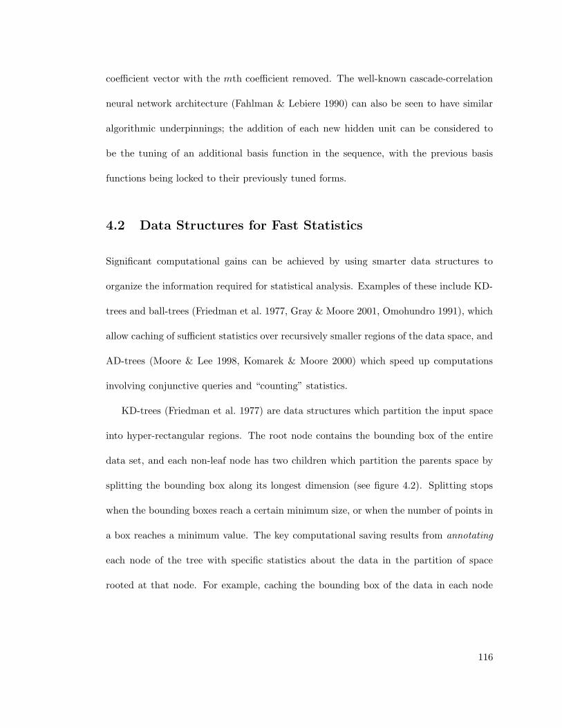
coefficient vector with the mth coefficient removed. The well-known cascade-correlation

neural network architecture (Fahlman & Lebiere 1990) can also be seen to have similar

algorithmic underpinnings; the addition of each new hidden unit can be considered to

be the tuning of an additional basis function in the sequence, with the previous basis

functions being locked to their previously tuned forms.

4.2 Data Structures for Fast Statistics

Significant computational gains can be achieved by using smarter data structures to

organize the information required for statistical analysis. Examples of these include KD-

trees and ball-trees (Friedman et al. 1977, Gray & Moore 2001, Omohundro 1991), which

allow caching of sufficient statistics over recursively smaller regions of the data space, and

AD-trees (Moore & Lee 1998, Komarek & Moore 2000) which speed up computations

involving conjunctive queries and “counting” statistics.

KD-trees (Friedman et al. 1977) are data structures which partition the input space

into hyper-rectangular regions. The root node contains the bounding box of the entire

data set, and each non-leaf node has two children which partition the parents space by

splitting the bounding box along its longest dimension (see figure 4.2). Splitting stops

when the bounding boxes reach a certain minimum size, or when the number of points in

a box reaches a minimum value. The key computational saving results from annotating

each node of the tree with specific statistics about the data in the partition of space

rooted at that node. For example, caching the bounding box of the data in each node

116

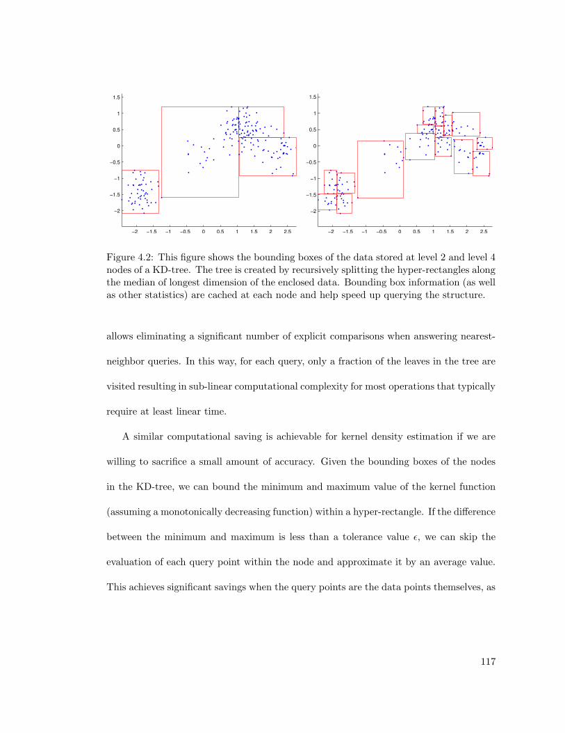
−2 −1.5 −1 −0.5 0 0.5 1 1.5 2 2.5

−2

−1.5

−1

−0.5

0

0.5

1

1.5

−2 −1.5 −1 −0.5 0 0.5 1 1.5 2 2.5

−2

−1.5

−1

−0.5

0

0.5

1

1.5

Figure 4.2: This figure shows the bounding boxes of the data stored at level 2 and level 4nodes of a KD-tree. The tree is created by recursively splitting the hyper-rectangles alongthe median of longest dimension of the enclosed data. Bounding box information (as wellas other statistics) are cached at each node and help speed up querying the structure.

allows eliminating a significant number of explicit comparisons when answering nearest-

neighbor queries. In this way, for each query, only a fraction of the leaves in the tree are

visited resulting in sub-linear computational complexity for most operations that typically

require at least linear time.

A similar computational saving is achievable for kernel density estimation if we are

willing to sacrifice a small amount of accuracy. Given the bounding boxes of the nodes

in the KD-tree, we can bound the minimum and maximum value of the kernel function

(assuming a monotonically decreasing function) within a hyper-rectangle. If the difference

between the minimum and maximum is less than a tolerance value ε, we can skip the

evaluation of each query point within the node and approximate it by an average value.

This achieves significant savings when the query points are the data points themselves, as

117

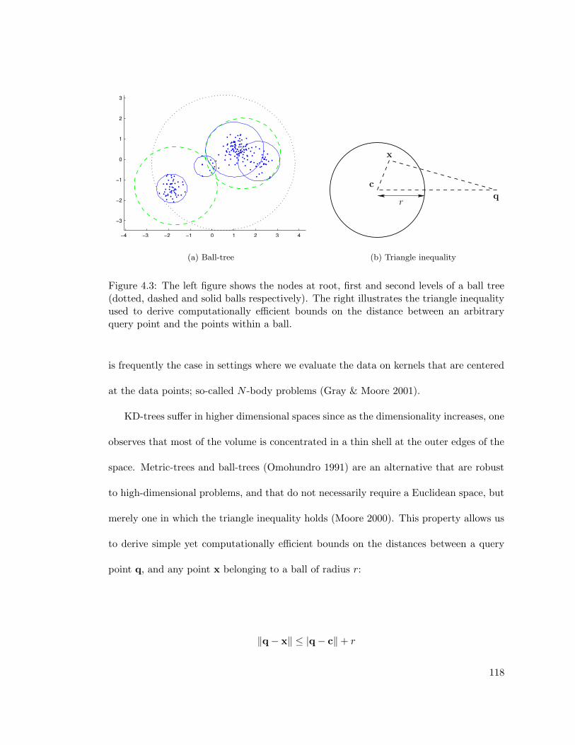
−4 −3 −2 −1 0 1 2 3 4

−3

−2

−1

0

1

2

3

(a) Ball-tree

x

q

c

r

(b) Triangle inequality

Figure 4.3: The left figure shows the nodes at root, first and second levels of a ball tree(dotted, dashed and solid balls respectively). The right illustrates the triangle inequalityused to derive computationally efficient bounds on the distance between an arbitraryquery point and the points within a ball.

is frequently the case in settings where we evaluate the data on kernels that are centered

at the data points; so-called N -body problems (Gray & Moore 2001).

KD-trees suffer in higher dimensional spaces since as the dimensionality increases, one

observes that most of the volume is concentrated in a thin shell at the outer edges of the

space. Metric-trees and ball-trees (Omohundro 1991) are an alternative that are robust

to high-dimensional problems, and that do not necessarily require a Euclidean space, but

merely one in which the triangle inequality holds (Moore 2000). This property allows us

to derive simple yet computationally efficient bounds on the distances between a query

point q, and any point x belonging to a ball of radius r:

‖q− x‖ ≤ |q− c‖+ r

118

‖q− x‖ ≥ |q− c‖ − r

These distance bounds are then used in a manner similar to the bounding boxes of

KD-trees to reduce the number of comparisons required to be performed with the actual

data points.

AD-trees (Moore & Lee 1998) are an efficient representation for statistical methods

which rely on “counting” occurrences of records satisfying sets of conjunctive queries

over the record attributes. Traditional representation schemes for such data include

precomputing answers to each query, which are stored in so-called contingency tables.

This method is useful in creating probability tables for Bayes nets, and in conjunctive

rule learning algorithms such as decision tree learning. Potential uses for statistical ma-

chine translation are obvious when we use the popular TF-IDF (term-frequency, inverse-

document-frequency) representation of documents.

AD-trees allow the precomputed answers to queries which are available in contingency

tables to be stored in a fraction of the memory requirements. For data sets in which

records arrive incrementally or in which the initial cost of constructing the AD-tree is too

high, an incremental version is also possible (Komarek & Moore 2000).

4.3 A Probabilistic Derivation of Backfitting

Consider the graphical model shown in figure 4.4(a). This model generalizes our discussion

in section 4.1, such that the input “dimensions” of figure 4.1 are replaced by arbitrary

119

Nfd(xi)

f2(xi)

f1(xi)

yi

ψy

b

(a) Graphical model forGeneralized Linear Regres-sion.

N

zi2

zi1

zid

f1(xi)

f2(xi)

fd(xi)

b1

b2

bd

yi ψy

(b) Graphical model for Probabilistic Backfit-ting.

Figure 4.4: We modify the original graphical model for generalized linear regression byinserting hidden variables zim in each branch of the fan-in. This modified model can besolved using the EM framework to derive a probabilistic version of backfitting.

basis functions fm(x) of the input — a model commonly known as generalized linear

regression (GLR) (Hastie & Tibshirani 1990). Our goal remains the same: given a data

set xD = (xi, yi)Ni=1, we wish to determine the most likely values of bm which linearly

combine the basis functions fm to generate the output y.

We also noted in section 4.1.2.2, that the backfitting family of algorithms is an efficient

set of methods which, under the right circumstances, is extremely robust since it requires

no expensive matrix inversion, and thus avoids the numerical pitfalls therein. A drawback

of the backfitting procedure is that it does not stem from a generative probabilistic

model, which limits its application in current Bayesian machine learning frameworks. In

this section we will describe how a probabilistic version of backfitting can be derived by

120

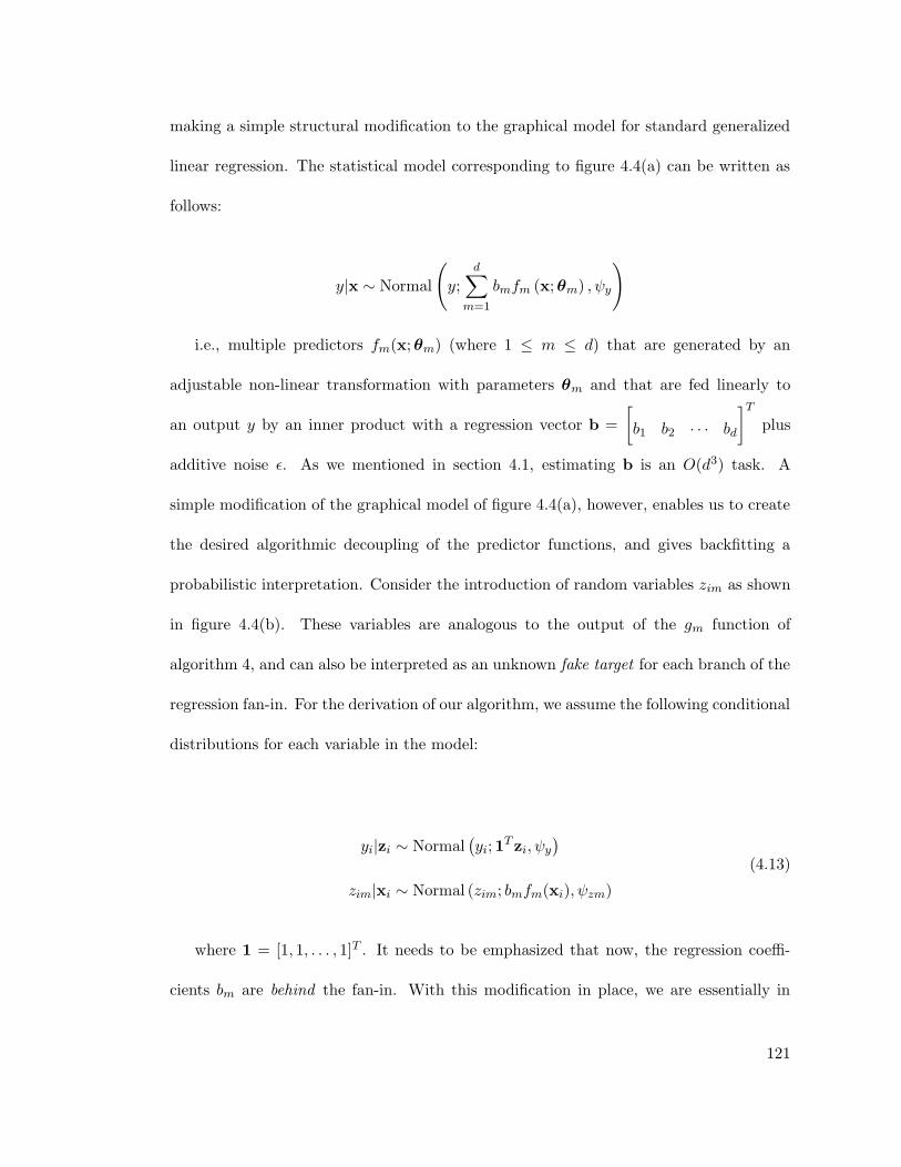
making a simple structural modification to the graphical model for standard generalized

linear regression. The statistical model corresponding to figure 4.4(a) can be written as

follows:

y|x ∼ Normal

(y;

d∑

m=1

bmfm (x;θm) , ψy

)

i.e., multiple predictors fm(x;θm) (where 1 ≤ m ≤ d) that are generated by an

adjustable non-linear transformation with parameters θm and that are fed linearly to

an output y by an inner product with a regression vector b =

[b1 b2 · · · bd

]Tplus

additive noise ε. As we mentioned in section 4.1, estimating b is an O(d3) task. A

simple modification of the graphical model of figure 4.4(a), however, enables us to create

the desired algorithmic decoupling of the predictor functions, and gives backfitting a

probabilistic interpretation. Consider the introduction of random variables zim as shown

in figure 4.4(b). These variables are analogous to the output of the gm function of

algorithm 4, and can also be interpreted as an unknown fake target for each branch of the

regression fan-in. For the derivation of our algorithm, we assume the following conditional

distributions for each variable in the model:

yi|zi ∼ Normal(yi; 1

T zi, ψy)

zim|xi ∼ Normal (zim; bmfm(xi), ψzm)

(4.13)

where 1 = [1, 1, . . . , 1]T . It needs to be emphasized that now, the regression coeffi-

cients bm are behind the fan-in. With this modification in place, we are essentially in

121

a situation where we wish to optimize the parameters φ =bm, ψzmdm=1 , ψy

, given

that we have observed variables xD = (xi, yi)Ni=1 and that we have unobserved vari-

ables xH = ziNi=1 in our graphical model. This situation fits very naturally into the

framework of maximum-likelihood estimation via the EM algorithm discussed in section

2.2.2.

4.3.1 An EM Algorithm for Probabilistic Backfitting

Given our modified statistical model represented by the graphical model of figure 4.4(b),

we wish to estimate the parameters bm and (possibly) optimize the individual functions

fm(x;θm) with respect to the parameters θm. This is easily formulated as an EM al-

gorithm, which maximizes the incomplete log likelihood ln p(xD;φ) which, from figure

4.4(a), can be expressed as:

ln p(xD;φ) = ln p(y|X; b,Ψz, ψy) = −N2

lnψy −1

2

N∑

i=1

(yi − bT f(xi)

)2+ const (4.14)

The EM algorithm however, operates by maximizing the expected complete log like-

lihood 〈ln p(xD,xH;φ)〉, where:

122

ln p(xD,xH;φ) = ln p(y,Z|X; b,Ψz, ψy)

= −N2

lnψy −1

2ψy

N∑

i=1

(yi − 1T zi

)2

−d∑

m=1

[N

2lnψzm +

1

2ψzm

N∑

i=1

(zim − bmfm(xi;θm)

)2]

+ const

(4.15)

Using the procedure outlined in section 2.2.2, we can derive (see appendix B.4) the

following EM update equations:

M-Step : E-Step :

bm =

∑Ni=1 〈zim〉 fm(xi)∑Ni=1 fm(xi)2

1TΣz1 =

(d∑

m=1

ψzm

)[1− 1

s

(d∑

m=1

ψzm

)]

ψy =1

N

N∑

i=1

(yi − 1T 〈zi〉

)2+ 1TΣz1 σ2

zm = ψzm

(1− 1

sψzm

)

ψzm =1

N

N∑

i=1

(〈zim〉 − bmfm(xi))2 + σ2

zm 〈zim〉 = bmfm(xi) +1

sψzm

(yi − bT f(xi)

)

where we define s ≡ ψy+∑d

m=1 ψzm. In addition, the parameters θm of each function

fm can be updated by setting:

N∑

i=1

(〈zim〉 − bmfm (xi;θm)

)∂fm (xi;θm)

∂θm= 0 (4.16)

123

and solving for θm. As this step depends on the particular choice of fm, e.g., splines,

kernel smoothers, parametric models, etc., we will not pursue it any further and just note

that any statistical approximation mechanism could be used.

Two items in the above EM algorithm are of special interest. First, all equations

in both the expectation and maximization steps are algorithmically O(d) where d is the

number of predictor functions fm. Second, if we substitute the expression for 〈zim〉 in the

maximization equation for bm we get the following update equation:

b(n+1)m = b(n)

m +ψzms

∑Ni=1

(yi−

∑dk=1 b

(n)k fk(xi)

)fm(xi)

∑Ni=1 fm(xi)2

(4.17)

Thus each EM cycle updates the mth regression coefficient by an amount proportional

to the correlation between the mth predictor and the residual error. Hence the residual

can be interpreted as forming a “fake target” for the mth branch of the fan-in. As the

next section shows, this enables us to place this algorithm in the context of backfitting.

4.3.2 Relating Traditional and Probabilistic Backfitting

To understand equation (4.17) as probabilistic backfitting, we note that backfitting can

be viewed as a formal Gauss-Seidel algorithm; an equivalence that becomes exact in

the special case of linear models (Hastie & Tibshirani 1990). For the linear system

FTFb = FTy, the Gauss-Seidel updates for the individual bm are:

bm =

∑Ni=1

(yi −

∑dk 6=m bkfk(xi)

)fm(xi)

∑Ni=1 fm(xi)2

(4.18)

124

Note that equation (4.18) — if used naively — only guarantees convergence for very

specially structured matrices. An extension to the Gauss-Seidel algorithm adds a fraction

(1− ω) of bm to the update and gives us the well-known relaxation algorithms:

b(n+1)m = (1− ω)b(n)

m + ω

∑Ni=1

(yi −

∑dk 6=m bkfk(xi)

)fm(xi)

∑Ni=1 fm(xi)2

(4.19)

which has improved convergence rates for over-relaxation (1 < ω < 2), or im-

proved stability for under-relaxation (0 < ω < 1). For ω = 1, the standard Gauss-

Seidel/backfitting of equation (4.18) is recovered. The appropriate value of ω which

allows the iterations to converge, while still maintaining a reasonable convergence rate

can only be determined by treating equation (4.18) as a discrete dynamical system, and

analyzing the eigenvalues of its system matrix — an O(d3) task. If however, we set

ω = ωm = ψzm/s in equation (4.19), it can be shown that (after some algebraic rear-

rangement,) we obtain exactly our EM update in equation (4.17), i.e., we indeed derive

a probabilistic version of backfitting.

It should be mentioned that a similar EM algorithm and model structure has been

proposed in the context of signal processing (Feder & Weinstein 1988), but we believe

this is the first time that the connection of this probabilistic derivation to the backfitting

algorithm has been demonstrated. As we will show in section 4.4, this allows us to

place this class of methods within a much wider framework of Bayesian model complexity

estimation.

125

4.3.3 Convergence of Probabilistic Backfitting

In general, for any maximum likelihood problem, the EM algorithm guarantees monotonic

increase in the incomplete likelihood, but does not guarantee that the final solution is the

global maximum. This section tries to answer the following questions:

1. What is the point of convergence of the probabilistic backfitting EM algorithm?

2. Are there local maxima (globally suboptimal solutions) in its likelihood space?

The answers to both questions depend on the fact that the incomplete likelihood

(or marginalized complete likelihood) function for linear regression in equation (4.14)

has a (possibly non-unique, but convex) global maximum corresponding to the OLS

solution of equation 4.2, but no local maxima. Could the introduction of the hidden

variables and additional parameters in equation (4.15) introduce local maxima in the

likelihood landscape? Note that for examining convergence properties, we only focus on

the estimation of the parameters φ = [b, ψz1, . . . , ψzd, ψy]T , as the functions fm cannot

be treated in general without knowing their structure. We start with the assumption that

we have reached a stationary point φ∗ in the EM algorithm, which implies:

∂ 〈ln p(y,Z|X;φ)〉∂φ

∣∣∣∣φ=φ∗

= 0 (4.20)

Using Jensen’s inequality, it is easy to show that for an arbitrary distribution Q(Z)

over the hidden variables:

ln p(y|X;φ) ≥ 〈ln p(y,Z|X;φ)〉Q(Z) +H [Q(Z)] = F(Q,φ) (4.21)

126

whereH [·] denotes entropy. EM performs a coordinate ascent; alternately maximizing

F w.r.t. Q (in the E-step) and φ (in the M-step). Differentiating F(Q,φ) w.r.t. φ at

the stationary point φ∗, and noting that the entropy term H [Q(Z)] is independent of φ,

gives:

∂F(Q,φ)

∂φ

∣∣∣∣φ=φ∗

=∂ 〈ln p(y,Z|X;φ)〉

∂φ

∣∣∣∣φ=φ∗

= 0 (4.22)

Note however, that the preceding E-step sets Q(Z) to the true posterior distribu-

tion p(Z|y,X;φ∗) which raises the lower bound in equation (4.21) to an equality —

i.e. ln p(y|X;φ) = F(Q,φ) — from which it follows that:

∂ ln p(y|X;φ)

∂φ

∣∣∣∣φ=φ∗

=∂F(Q,φ)

∂φ

∣∣∣∣φ=φ∗

= 0 (4.23)

i.e. we have reached a maximum in the incomplete likelihood as well. Given that the

incomplete log likelihood ln p(y|X;φ) in equation (4.14) has only a global maximum (i.e.,

the OLS solution), reaching the stationary point of equation (4.20) in our EM algorithm

for probabilistic backfitting must correspond to finding the OLS solution. Therefore,

probabilistic backfitting is indeed performing true linear regression with a global optimum.

4.4 Bayesian Backfitting

Having a probabilistic interpretation of backfitting, allows us to use a Bayesian framework

to regularize its OLS solution against overfitting. We achieve this by placing a prior

127

N

d

ψy

bm

ψm

yizim

α

aα bα

fm(xi)

(a) Graphical model for backfitting withshrinkage prior

−2

0

2 −20

2

0.020.040.060.08

0.10.120.14

b2

Marginal with common precision

b1

(b) Resulting marginal prior over b

Figure 4.5: By associating a single Gamma distributed precision with the regressionvector, we create a marginal prior over b that favors minimum-norm solutions, similar toshrinkage methods such as ridge regression.

distribution over the regression coefficients b. As the following two sections demonstrate,

our choice of prior structure results in two different, yet important forms of regularization.

4.4.1 Regularizing the Regression Vector Length

The graphical model for our first form of Bayesian prior is shown in figure 4.5(a). A

Gaussian prior is placed over the regression coefficient vector b such that the variance of

this prior is controlled by a single precision parameter α. Our uncertainty in the value of

this prior precision is in turn represented by a broad Gamma distribution over α.

128

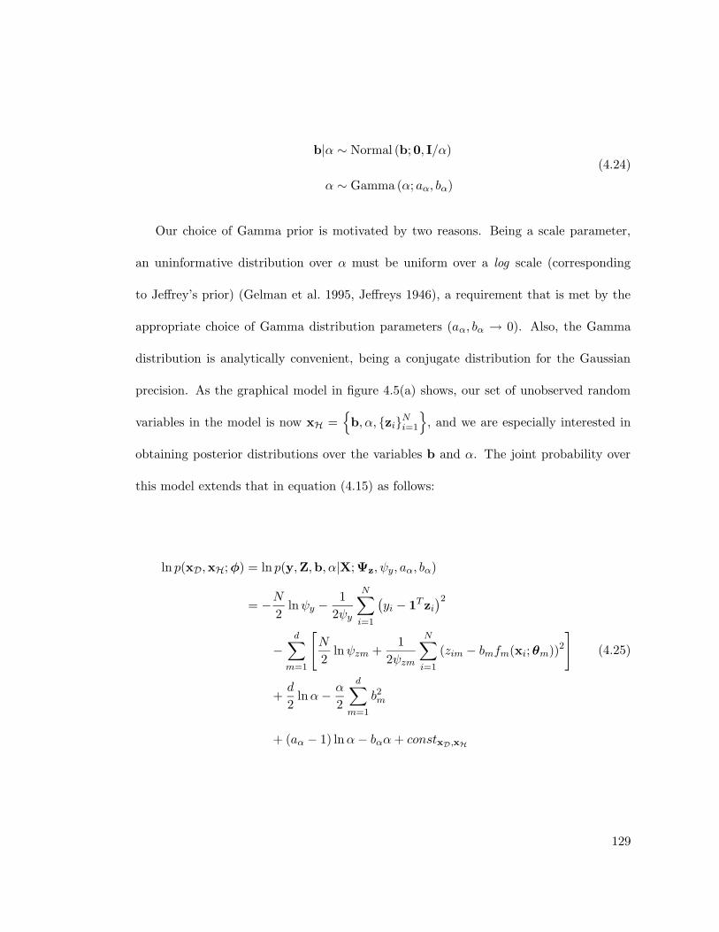
b|α ∼ Normal (b; 0, I/α)

α ∼ Gamma (α; aα, bα)

(4.24)

Our choice of Gamma prior is motivated by two reasons. Being a scale parameter,

an uninformative distribution over α must be uniform over a log scale (corresponding

to Jeffrey’s prior) (Gelman et al. 1995, Jeffreys 1946), a requirement that is met by the

appropriate choice of Gamma distribution parameters (aα, bα → 0). Also, the Gamma

distribution is analytically convenient, being a conjugate distribution for the Gaussian

precision. As the graphical model in figure 4.5(a) shows, our set of unobserved random

variables in the model is now xH =

b, α, ziNi=1

, and we are especially interested in

obtaining posterior distributions over the variables b and α. The joint probability over

this model extends that in equation (4.15) as follows:

ln p(xD,xH;φ) = ln p(y,Z,b, α|X; Ψz, ψy, aα, bα)

= −N2

lnψy −1

2ψy

N∑

i=1

(yi − 1T zi

)2

−d∑

m=1

[N

2lnψzm +

1

2ψzm

N∑

i=1

(zim − bmfm(xi;θm))2

]

+d

2lnα− α

2

d∑

m=1

b2m

+ (aα − 1) lnα− bαα+ constxD,xH

(4.25)

129

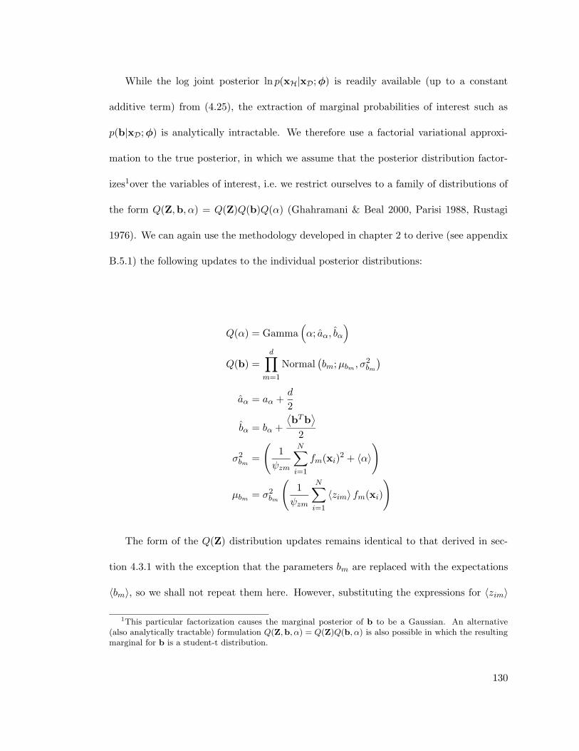
While the log joint posterior ln p(xH|xD;φ) is readily available (up to a constant

additive term) from (4.25), the extraction of marginal probabilities of interest such as

p(b|xD;φ) is analytically intractable. We therefore use a factorial variational approxi-

mation to the true posterior, in which we assume that the posterior distribution factor-

izes1over the variables of interest, i.e. we restrict ourselves to a family of distributions of

the form Q(Z,b, α) = Q(Z)Q(b)Q(α) (Ghahramani & Beal 2000, Parisi 1988, Rustagi

1976). We can again use the methodology developed in chapter 2 to derive (see appendix

B.5.1) the following updates to the individual posterior distributions:

Q(α) = Gamma(α; aα, bα

)

Q(b) =d∏

m=1

Normal(bm;µbm , σ

2bm

)

aα = aα +d

2

bα = bα +

⟨bTb

⟩

2

σ2bm =

(1

ψzm

N∑

i=1

fm(xi)2 + 〈α〉

)

µbm = σ2bm

(1

ψzm

N∑

i=1

〈zim〉 fm(xi)

)

The form of the Q(Z) distribution updates remains identical to that derived in sec-

tion 4.3.1 with the exception that the parameters bm are replaced with the expectations

〈bm〉, so we shall not repeat them here. However, substituting the expressions for 〈zim〉

1This particular factorization causes the marginal posterior of b to be a Gaussian. An alternative(also analytically tractable) formulation Q(Z,b, α) = Q(Z)Q(b, α) is also possible in which the resultingmarginal for b is a student-t distribution.

130

in the update equations for the distribution of Q(b) gives us the following update for the

regression coefficients:

〈bm〉(n+1) =

( ∑Ni=1 fm(xi)

2

∑Ni=1 fm(xi)2 + ψzm 〈α〉

)〈bm〉(n)

+ψzms

∑Ni=1

(yi −

∑dk=1 〈bk〉(n) fk(xi)

)fm(xi)

(∑Ni=1 fm(xi)2 + ψzm 〈α〉

) (4.26)

Comparing this solution with the result derived for probabilistic backfitting in equa-

tion (4.17), we see that in absence of correlation between the residual error, and the k-th

predictor fk(x), the first term of equation (4.26) automatically decays the corresponding

regression coefficient to zero. This is similar in effect to shrinkage methods such as ridge

regression.

Note however, that the structure of the marginal prior over the regression coefficients b

in figure 4.5(b) suggests that solutions closer to the origin are favored. In fact, sharing the

common precision variable α across all the regression coefficients results in a regularized

solution which minimizes the norm ‖b‖2 of the entire regression vector, which is in fact

identical to a ridge regression solution with a single ridge parameter. In our formulation

however, the estimation of the “correct” value of the ridge parameter is implicitly inferred

without the need for traditionally expensive cross-validation techniques.

This form of regularization is particularly useful when there are groups of inputs

supplying redundant information (for robustness across sensors, for example), since the

131

N

d

ψy

bm

ψm

yizim

αm

aα bα

fm(xi)

(a) Graphical model with ARD prior

−2

0

2 −20

2

2468

1012

x 10−3

b2

Marginal with individual precisions

b1

(b) Resulting marginal prior over b

Figure 4.6: By associating an individual Gamma distributed precision with each regres-sion coefficient, we create a marginal prior over b that favors sparse solutions which liealong the (hyper)-spines of the distribution.

regression solution tends to distribute the responsibility for the output inference over all

relevant input dimensions.

4.4.2 Regularizing the Number of Relevant Inputs

Modifying figure 4.5(a) slightly, we now place individual precision variables αm over each

of the regression parameters bm, resulting in figure 4.6(a). This model structure can be

captured by the following set of prior distributions:

b|α ∼d∏

m=1

Normal (bm; 0, 1/αm)

α ∼d∏

m=1

Gamma (α; aα, bα)

(4.27)

132

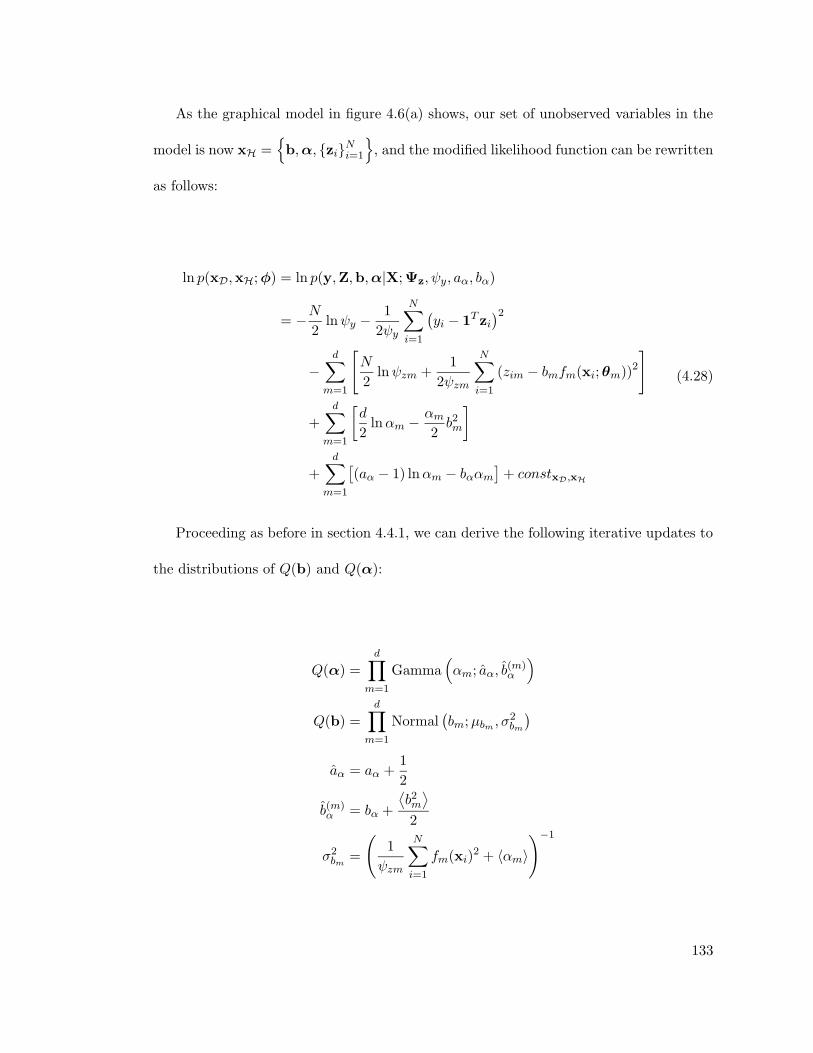
As the graphical model in figure 4.6(a) shows, our set of unobserved variables in the

model is now xH =

b,α, ziNi=1

, and the modified likelihood function can be rewritten

as follows:

ln p(xD,xH;φ) = ln p(y,Z,b,α|X; Ψz, ψy, aα, bα)

= −N2

lnψy −1

2ψy

N∑

i=1

(yi − 1T zi

)2

−d∑

m=1

[N

2lnψzm +

1

2ψzm

N∑

i=1

(zim − bmfm(xi;θm))2

]

+d∑

m=1

[d

2lnαm −

αm2b2m

]

+d∑

m=1

[(aα − 1) lnαm − bααm

]+ constxD,xH

(4.28)

Proceeding as before in section 4.4.1, we can derive the following iterative updates to

the distributions of Q(b) and Q(α):

Q(α) =d∏

m=1

Gamma(αm; aα, b

(m)α

)

Q(b) =d∏

m=1

Normal(bm;µbm , σ

2bm

)

aα = aα +1

2

b(m)α = bα +

⟨b2m⟩

2

σ2bm =

(1

ψzm

N∑

i=1

fm(xi)2 + 〈αm〉

)−1

133

µbm = σ2bm

(1

ψzm

N∑

i=1

〈zim〉 fm(xi)

)

Deriving our update equation for the mean of the regression coefficients as we did in

equation (4.26), we get:

〈bm〉(n+1) =

( ∑Ni=1 fm(xi)

2

∑Ni=1 fm(xi)2 + ψzm 〈αm〉

)〈bm〉(n)

+ψzms

∑Ni=1

(yi −

∑dk=1 〈bk〉(n) fk(xi)

)fm(xi)

(∑Ni=1 fm(xi)2 + ψzm 〈αm〉

) (4.29)

This solution is almost identical to that of equation (4.26), except that because of

the individual precision variables, the regularization of the regression solution occurs

over the magnitude of each regression coefficient, rather than the overall norm. This

results in a regression solution that minimizes the number of relevant inputs required

to accurately predict the output, much like the automatic relevance detection (ARD)

framework in neural networks (Neal 1994). This is also intuitively apparent from the

marginal prior over b shown in figure 4.6(b), which favors sparse solutions which lie

along the (hyper-)spines of the distribution.

While the regularization discussed in the previous section is useful in situations where

there exists redundant information, this form of regularization is desirable when the input

contains information that is irrelevant to predicting the output.

Note that the graphical models of figures 4.5(a) and 4.6(a) are two extremes in a

spectrum of regularization options. One can certainly conceive of models in which groups

134

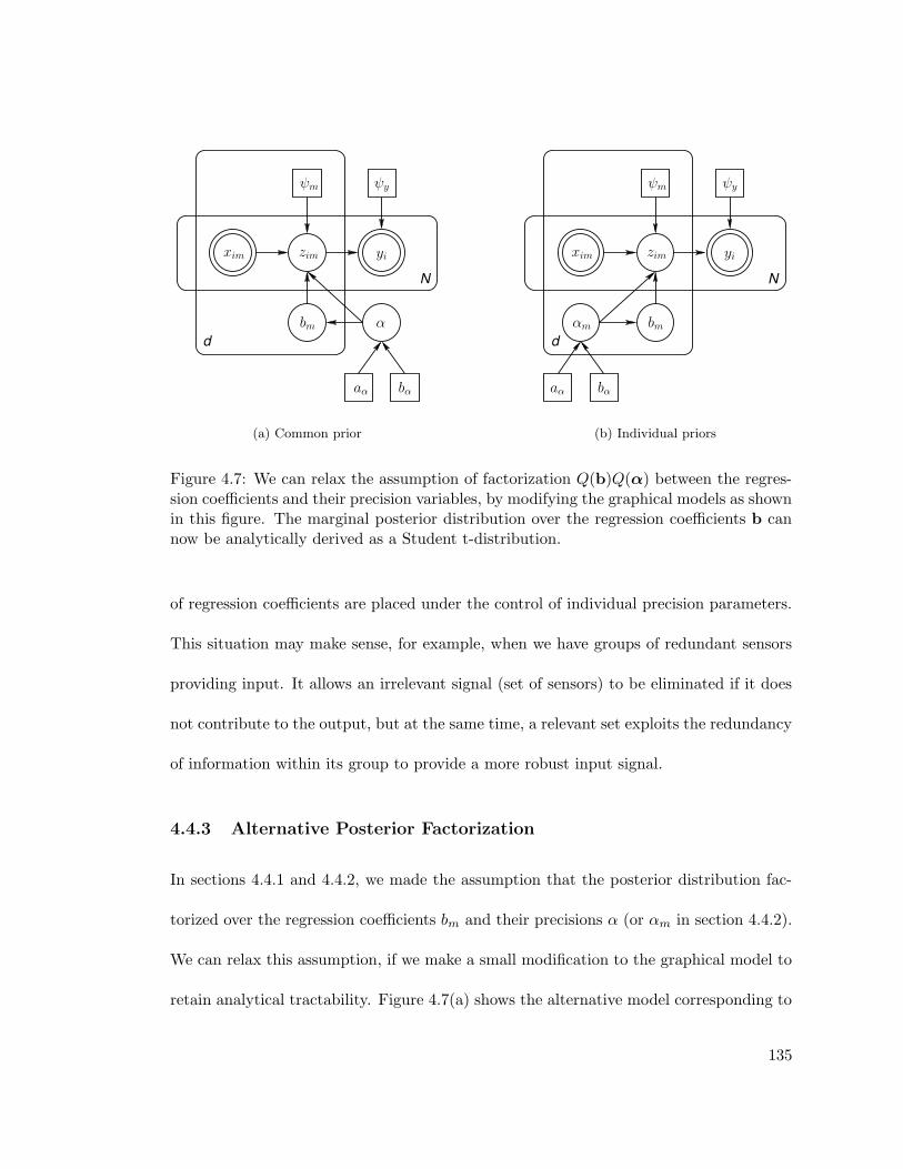
N

d

ψy

bm

ψm

yizimxim

α

aα bα

(a) Common prior

N

d

ψy

bm

ψm

yizimxim

αm

aα bα

(b) Individual priors

Figure 4.7: We can relax the assumption of factorization Q(b)Q(α) between the regres-sion coefficients and their precision variables, by modifying the graphical models as shownin this figure. The marginal posterior distribution over the regression coefficients b cannow be analytically derived as a Student t-distribution.

of regression coefficients are placed under the control of individual precision parameters.

This situation may make sense, for example, when we have groups of redundant sensors

providing input. It allows an irrelevant signal (set of sensors) to be eliminated if it does

not contribute to the output, but at the same time, a relevant set exploits the redundancy

of information within its group to provide a more robust input signal.

4.4.3 Alternative Posterior Factorization

In sections 4.4.1 and 4.4.2, we made the assumption that the posterior distribution fac-

torized over the regression coefficients bm and their precisions α (or αm in section 4.4.2).

We can relax this assumption, if we make a small modification to the graphical model to

retain analytical tractability. Figure 4.7(a) shows the alternative model corresponding to

135

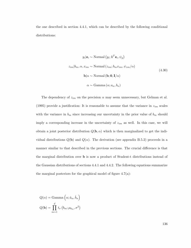
the one described in section 4.4.1, which can be described by the following conditional

distributions:

yi|zi ∼ Normal(yi; 1

T zi, ψy)

zim|bm, α, xim ∼ Normal (zim; bmxim, ψzm/α)

b|α ∼ Normal (b; 0, I/α)

α ∼ Gamma (α; aα, bα)

(4.30)

The dependency of zim on the precision α may seem unnecessary, but Gelman et al.

(1995) provide a justification: It is reasonable to assume that the variance in zim scales

with the variance in bm since increasing our uncertainty in the prior value of bm should

imply a corresponding increase in the uncertainty of zim as well. In this case, we will

obtain a joint posterior distribution Q(b, α) which is then marginalized to get the indi-

vidual distributions Q(b) and Q(α). The derivation (see appendix B.5.2) proceeds in a

manner similar to that described in the previous sections. The crucial difference is that

the marginal distribution over b is now a product of Student-t distributions instead of

the Gaussian distributions of sections 4.4.1 and 4.4.2. The following equations summarize

the marginal posteriors for the graphical model of figure 4.7(a):

Q(α) = Gamma(α; aα, bα

)

Q(b) =d∏

m=1

tν(bm;µbm , σ

2)

136

aα = aα +Nd

2

bα = bα +

d∑

m=1

1

2ψzm

N∑

i=1

⟨z2im

⟩−(

N∑

i=1

fm(xi)2 + ψzm

)−1( N∑

i=1

〈zim〉 fm(xi)

)2

ν = 2aα

µbm =

(N∑

i=1

fm(xi)2 + ψzm

)−1( N∑

i=1

〈zim〉 fm(xi)

)

σ2bm =

bαψzmaα

(N∑

i=1

fm(xi)2 + ψzm

)−1

For the case of individual precision variables αm shown in figure 4.7(b), we have the

following updates:

Q(α) =d∏

m=1

Gamma(αm; aα, b

(m)α

)

Q(b) =d∏

m=1

tν(bm;µbm , σ

2)

aα = aα +N

2

b(m)α = bα +

1

2ψzm

N∑

i=1

⟨z2im

⟩−(

N∑

i=1

fm(xi)2 + ψzm

)−1( N∑

i=1

〈zim〉 fm(xi)

)2

ν = 2aα

µbm =

(N∑

i=1

fm(xi)2 + ψzm

)−1( N∑

i=1

〈zim〉 fm(xi)

)

σ2bm =

b(m)α ψzmaα

(N∑

i=1

fm(xi)2 + ψzm

)−1

137

−10 −5 0 5 100

0.2

0.4

0.6

0.8

1

−10 −5 0 5 10−14

−12

−10

−8

−6

−4

−2

0

Figure 4.8: The left panel shows the logistic function (solid thick line), and two approx-imations with the variational parameters set to ξ = 3 (dashed line), and ξ = 7 (solidthin line). The points of tangency between the true function and the approximation arecircled. The center panel shows the same plots on a log scale, while the right panel showsthe classification solution to a toy problem.

This approximation can be used in conjunction with a distribution over the noise

parameter ψy to derive a form of robust regression which is less sensitive to outliers

than our original formulation, in which the predictive distribution over the output is a

Gaussian.

4.4.4 Extension to Classification

The probabilistic backfitting EM algorithm that was developed in section 4.3.1 can be

adapted to handle categorical outputs yi ∈ −1,+1 by simply changing the target

conditional distribution p(yi|zi) in equation (4.13) to a Bernoulli distribution via the

sigmoid link function g(x) =(1 + exp(−x)

)−1. In this case, the conditional distribution

can be expressed as:

p(yi|zi) =1

1 + exp (−yi1T zi)= g(yi1

T zi)

138

Since this renders the posterior intractable due to non-conjugacy with p(zi|xi), we

follow (Jaakkola & Jordan 2000) and introduce an additional lower bound using the

inequality:

g(x) ≥ g(ξ) exp

x− ξ

2− ϕ(ξ)

(x2 − ξ2

)

where ϕ(ξ) = tan(ξ/2)/4ξ, and ξ is the variational parameter for the family of lower

bounds to g(x) (see figure 4.8). Hence we can lower bound the likelihood p(yi|zi) by the

parameterized version p(yi|zi, ξi) as follows:

p(yi|zi) = g(yi1T zi)

≥ p(yi|zi; ξi)

= g(ξi) exp

yi1

T zi − ξi2

− ϕ(ξi)(zTi 11T zi − ξ2

i

)(4.31)

Note that this form still is an exponent of a quadratic in zi which retains conjugacy

with p(zi|b; xi), and allows us to proceed with our EM derivation as before, with the

additional step that we must optimize the ξi parameters. We again start by writing out

the log complete likelihood, which is the joint distribution over the known and unknown

variables xD and xH in the model:

139

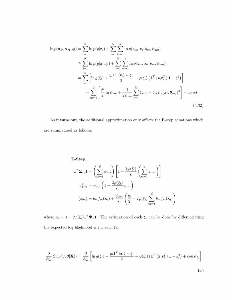
ln p(xD,xH;φ) =N∑

i=1

ln p(y|zi) +N∑

i=1

d∑

m=1

ln p(zim|xi; bm, ψzm)

≥N∑

i=1

ln p(y|zi; ξi) +N∑

i=1

d∑

m=1

ln p(zim|xi; bm, ψzm)

=N∑

i=1

[ln g(ξi) +

yi1T 〈zi〉 − ξi

2− ϕ(ξi)

(1T⟨ziz

Ti

⟩1− ξ2

i

)]

−d∑

m=1

[N

2lnψzm +

1

2ψzm

N∑

i=1

(zim − bmfm(xi;θm))2

]+ const

(4.32)

As it turns out, the additional approximation only affects the E-step equations which

are summarized as follows:

E-Step :

1TΣzi1 =

(d∑

m=1

ψzm

)[1− 2ϕ(ξi)

si

(d∑

m=1

ψzm

)]

σ2zim = ψzm

(1− 2ϕ(ξi)

siψzm

)

〈zim〉 = bmfm(xi) +ψzmsi

(yi2− 2ϕ(ξi)

d∑

m=1

bmfm(xi)

)

where si = 1 + 2ϕ(ξi)1TΨz1. The estimation of each ξi can be done by differentiating

the expected log likelihood w.r.t. each ξi:

∂

∂ξi〈ln p(y,θ|X)〉 =

∂

∂ξi

[ln g(ξi) +

yi1T 〈zi〉 − ξi

2− ϕ(ξi)

(1T⟨ziz

Ti

⟩1− ξ2

i

)+ constξi

]

140

= 1− g(ξi)−1

2+ 2ξiϕ(ξi)

︸ ︷︷ ︸=0

−∂ϕ(ξi)

∂ξi

(1T⟨ziz

Ti

⟩1− ξ2

i

)

Hence the likelihood is maximized by solving the following:

∂ϕ(ξi)

∂ξi

(1T⟨ziz

Ti

⟩1− ξ2

i

)= 0

which has solutions at ∂ϕ(ξi)/∂ξi = 0 and at ξ2i = 1T

⟨ziz

Ti

⟩1. One can show that

the solution ∂ϕ(ξi)/∂ξi = 0 occurs for the value ξi = 0, and actually corresponds to a

minimum rather than a maximum of the expected log likelihood. Hence we have the

admissible solutions for ξi being:

ξi = ±√

1T⟨zizTi

⟩1

The sign of ξi can be chosen arbitrarily, since the likelihood is an even function of ξi,

i.e. both solutions result in the likelihood taking the same maximal value (c.f. figure 4.8).

Importantly, the O(d) complexity of all update equations is preserved even in the exten-

sion to categorical output data, making backfitting for classification an equally robust

and efficient tool as its regression counterpart.

4.4.4.1 Bayesian Backfitting for Classification

Given that the functional approximation of equation (4.31) allows us to retain the con-

jugacy necessary for an analytical treatment, the Bayesian extensions of section 4.4 are

141

straightforward to apply to our classification model. For the case in which we have a com-

mon shared precision parameter α across all regression parameters (c.f. section 4.4.1), the

bm variables still have a posterior Gaussian with the mean update as follows:

〈bm〉(n+1) =

( ∑Ni=1 fm(xi)

2

∑Ni=1 fm(xi)2 + ψzm 〈α〉

)〈bm〉(n)

+ψzm

∑Ni=1

1si

(yi2 − 2ϕ(ξi)〈b〉(n)T f(xi)

)fm(xi)

(∑Ni=1 fm(xi)2 + ψzm 〈α〉

)

For the case in which we have an individual precision parameter αm over each regres-

sion parameter (c.f. section 4.4.2), the bm variables again have a posterior Gaussian with

the mean update as follows:

〈bm〉(n+1) =

( ∑Ni=1 fm(xi)

2

∑Ni=1 fm(xi)2 + ψzm 〈αm〉

)〈bm〉(n)

+ψzm

∑Ni=1

1si

(yi2 − 2ϕ(ξi)〈b〉(n)T f(xi)

)fm(xi)

(∑Ni=1 fm(xi)2 + ψzm 〈αm〉

)

4.4.5 Efficient Sparse Bayesian Learning and RVMs

The relevance vector machine was introduced by Tipping (2000) as an alternative to the

popular support vector regression (SVR) method. The RVM operates in a framework

similar to generalized linear regression, but uses the following generative model:

y(x; b) =N∑

i=1

bik(x,xi) + ε (4.33)

142

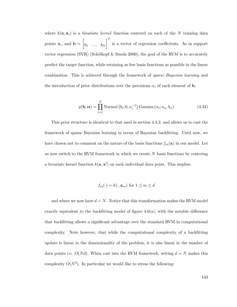
where k(x,xi) is a bivariate kernel function centered on each of the N training data

points xi, and b =

[b1 . . . bN

]Tis a vector of regression coefficients. As in support

vector regression (SVR) (Scholkopf & Smola 2000), the goal of the RVM is to accurately

predict the target function, while retaining as few basis functions as possible in the linear

combination. This is achieved through the framework of sparse Bayesian learning and

the introduction of prior distributions over the precisions αi of each element of b:

p(b,α) =N∏

i=1

Normal(bi; 0, α−1

i

)Gamma (αi; aα, bα) (4.34)

This prior structure is identical to that used in section 4.4.2, and allows us to cast the

framework of sparse Bayesian learning in terms of Bayesian backfitting. Until now, we

have chosen not to comment on the nature of the basis functions fm(x) in our model. Let

us now switch to the RVM framework in which we create N basis functions by centering

a bivariate kernel function k(x,x′) on each individual data point. This implies:

fm(·) = k(·,xm) for 1 ≤ m ≤ d

and where we now have d = N . Notice that this transformation makes the RVM model

exactly equivalent to the backfitting model of figure 4.6(a), with the notable difference

that backfitting allows a significant advantage over the standard RVM in computational

complexity. Note however, that while the computational complexity of a backfitting

update is linear in the dimensionality of the problem, it is also linear in the number of

data points i.e. O(Nd). When cast into the RVM framework, setting d = N makes this

complexity O(N2). In particular we would like to stress the following:

143

• At each update of the αm hyperparameters, the RVM requires an O(N 3) Cholesky

decomposition to re-estimate the regression parameters, while discarding the es-

timate at the previous iteration. In the backfitting-RVM however, the existing

estimate of the regression parameters provides a good starting estimate, allowing

the update to complete in just a handful of O(N 2) iterations (∼ 10 iterations were

sufficient in our simulations). The saving in computation is especially evident when

the number of data points (and hence the effective dimensionality) is large, and in

situations where the hyperparameters require many updates before convergence.

• In the initial computations within the graphical model, it seems wasteful to spend

large amounts of computation on estimating parameters accurately, when surround-

ing parameters (and hyperparameters) have not converged. One can structure the

backfitting updates to work with partially converged estimates, such that the brunt

of computation is only expended to accurately estimate a variable when one is more

confident about the variables in its Markov blanket.

Figure 4.9 shows backfitting-RVM used to fit a toy data set generated using the 1-

dimensional sinc function sin(x)/x, as well as the popular “Banana” classification dataset

(Ratsch, Onoda & Muller 2001) using the Gaussian kernel:

k(xi, xj) = exp−λ (xi − xj)2

for λ > 0. Even though backfitting-RVM is an order of magnitude faster than the

standard RVM, it suffers no penalty in generalization error or its ability to sparsify the

set of basis functions. Note that Tipping (2001) proposes an optimization of the distance

144

−10 −8 −6 −4 −2 0 2 4 6 8 10−0.4

−0.2

0

0.2

0.4

0.6

0.8

1 trueapproximatedtrainingrelevant

(a) Fitting the sinc function

−2 −1.5 −1 −0.5 0 0.5 1 1.5 2

−1.5

−1

−0.5

0

0.5

1

1.5

2

2.5class 1class 2relevant vectors

(b) Fitting the banana dataset

Figure 4.9: Fitting the sinc function using backfitting-RVM.

metric λ that is based on gradient ascent in the log likelihood. Such a gradient can also

be computed for backfitting as:

∂ 〈ln p(y,Z|X)〉∂λ

=N∑

j=1

bjψzj

N∑

i=1

(〈zij〉 − bjkij) (xi − xj)2 kij

where we have abbreviated kij = k(xi, xj). Based on our experience however, we

would like to caution against unconstrained maximization of the likelihood, especially

over distance metrics. Instead, we would recommend the route taken in the Gaussian

process community, which is to treat these variables as hyperparameters, and place prior

distributions over them. Exact solutions being typically intractable, we can either opti-

mize them by using maximum a posteriori estimates (MacKay 1999), or by Monte Carlo

techniques (Williams & Rasmussen 1996). Note that although a change in the distance

metric would require a re-evaluation of the kernel responses at each data point, such

computations can be speeded up significantly by the techniques reviewed in section 4.2.

145

Other optimizations suggested (Tipping 2001, Tipping & Faul 2003) include pruning

the basis functions when their precision variables dictate that they are unneeded, as well

as adopting a greedy (but potentially suboptimal) strategy in which the algorithm starts

with a single basis function and adds candidates as necessary. We would like to emphasize

that our implementation of the backfitting-RVM performs neither of these optimizations,

although it is trivial to introduce them into our framework as well. Other variants of the

RVM exist including a sequential version (Vermaak et al. 2004) which relies on generalized

importance sampling to determine the number of kernels and their centers.

4.5 Bayesian Backfitting Experiments

We compare the use of partial least squares (PLS) and Bayesian backfitting as described

in section 4.4.2 to analyze the following real-world data set collected from neuroscience.

Our choice of PLS for comparison was motivated by the fact that this is a well-studied

algorithm that also has O(d) complexity, and is widely used on data sets in chemometrics

with similar properties. The data set consists of simultaneous recordings (2400 data

points) of firing-rate coded activity in 71 motor cortical neurons and the EMG of 11

muscles. The goal is to determine which neurons are responsible for the activity of each

muscle. The relationship between neural and muscle activity is assumed to be linear,

such that the basis functions in backfitting are simply a copy of the respective input

dimensions, i.e. fm(x) = xm.

A brute-force study (conducted by our research collaborators) painstakingly consid-

ered every possible combination of neurons (up to groups of 20 for computational reasons,

146

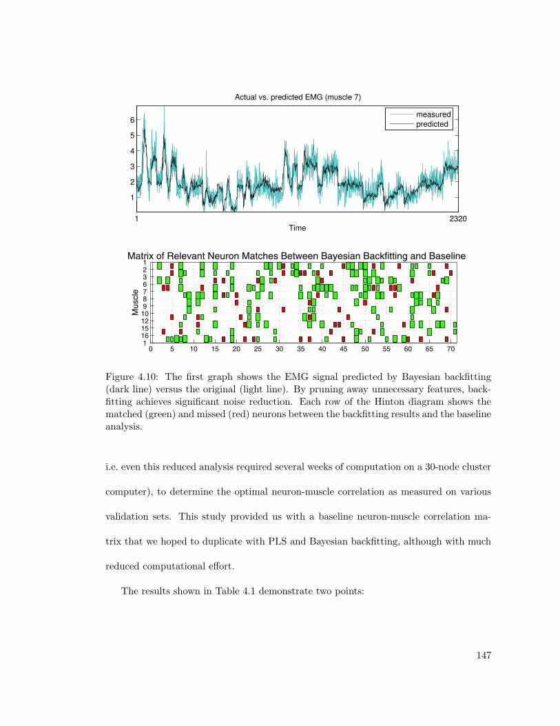
1 2320

1

2

3

4

5

6

Time

Actual vs. predicted EMG (muscle 7)

measuredpredicted

Figure 4.10: The first graph shows the EMG signal predicted by Bayesian backfitting(dark line) versus the original (light line). By pruning away unnecessary features, back-fitting achieves significant noise reduction. Each row of the Hinton diagram shows thematched (green) and missed (red) neurons between the backfitting results and the baselineanalysis.

i.e. even this reduced analysis required several weeks of computation on a 30-node cluster

computer), to determine the optimal neuron-muscle correlation as measured on various

validation sets. This study provided us with a baseline neuron-muscle correlation ma-

trix that we hoped to duplicate with PLS and Bayesian backfitting, although with much

reduced computational effort.

The results shown in Table 4.1 demonstrate two points:

147

Bayes. back. PLS baseline

neuron match 93.6% 18% —

nMSE 0.8446 1.77 0.84

Table 4.1: Results on the neuron-muscle data set

• The relevant neurons found by Bayesian backfitting contained over 93% of the

neurons found by the baseline study, while PLS fails to find comparable correlations.

The neuron match in backfitting is easily inferred from the resulting magnitude of

the precision parameters α, while for PLS, the neuron match was inferred based on

the subspace spanned by the projections that PLS employed.

• The regression accuracy of Bayesian backfitting (as determined by 8-fold cross-

validation), is comparable to that of the baseline study, while PLS’ failure to find

the correct correlations causes it to have significantly higher generalization errors.

The analysis for both backfitting and PLS was carried out using the same validation

sets as those used for the baseline analysis.

The performance of Bayesian backfitting on this particularly difficult data set shows

that it is a viable alternative to traditional generalized linear regression tools. Even with

the additional Bayesian inference for ARD, it maintains its algorithmic efficiency since

no matrix inversion is required.

As an aside it is useful to note that Bayesian backfitting and PLS required of the

order of 8 hours of computation on a standard PC2 (compared with several weeks on a

cluster for the brute-force study), and evaluated the contributions of all 71 neurons.

2Pentium IV class machine, 1.7GHz

148

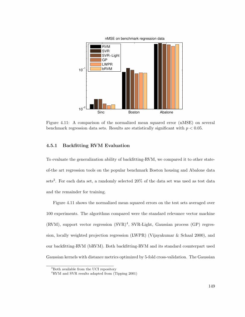
Sinc Boston Abalone10−2

10−1

nMSE on benchmark regression data

RVMSVRSVR−LightGPLWPRbRVM

Figure 4.11: A comparison of the normalized mean squared error (nMSE) on severalbenchmark regression data sets. Results are statistically significant with p < 0.05.

4.5.1 Backfitting RVM Evaluation

To evaluate the generalization ability of backfitting-RVM, we compared it to other state-

of-the art regression tools on the popular benchmark Boston housing and Abalone data

sets3. For each data set, a randomly selected 20% of the data set was used as test data

and the remainder for training.

Figure 4.11 shows the normalized mean squared errors on the test sets averaged over

100 experiments. The algorithms compared were the standard relevance vector machine

(RVM), support vector regression (SVR)4, SVR-Light, Gaussian process (GP) regres-

sion, locally weighted projection regression (LWPR) (Vijayakumar & Schaal 2000), and

our backfitting-RVM (bRVM). Both backfitting-RVM and its standard counterpart used

Gaussian kernels with distance metrics optimized by 5-fold cross-validation. The Gaussian

3Both available from the UCI repository4RVM and SVR results adapted from (Tipping 2001)

149

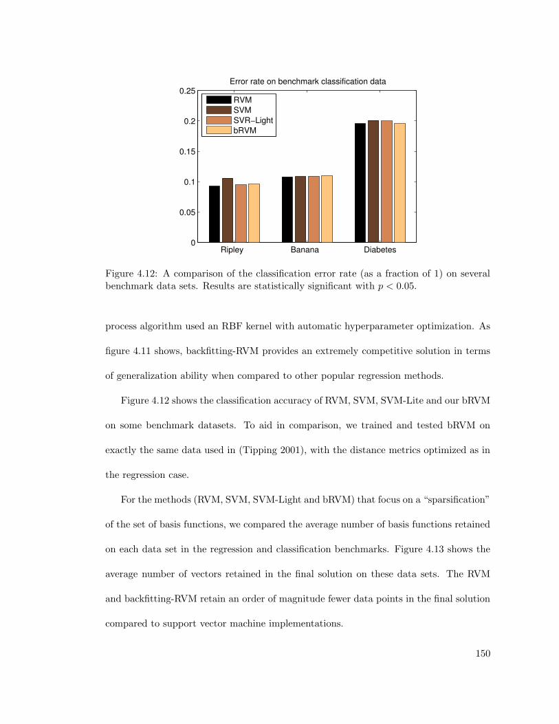
Ripley Banana Diabetes0

0.05

0.1

0.15

0.2

0.25Error rate on benchmark classification data

RVMSVMSVR−LightbRVM

Figure 4.12: A comparison of the classification error rate (as a fraction of 1) on severalbenchmark data sets. Results are statistically significant with p < 0.05.

process algorithm used an RBF kernel with automatic hyperparameter optimization. As

figure 4.11 shows, backfitting-RVM provides an extremely competitive solution in terms

of generalization ability when compared to other popular regression methods.

Figure 4.12 shows the classification accuracy of RVM, SVM, SVM-Lite and our bRVM

on some benchmark datasets. To aid in comparison, we trained and tested bRVM on

exactly the same data used in (Tipping 2001), with the distance metrics optimized as in

the regression case.

For the methods (RVM, SVM, SVM-Light and bRVM) that focus on a “sparsification”

of the set of basis functions, we compared the average number of basis functions retained

on each data set in the regression and classification benchmarks. Figure 4.13 shows the

average number of vectors retained in the final solution on these data sets. The RVM

and backfitting-RVM retain an order of magnitude fewer data points in the final solution

compared to support vector machine implementations.

150

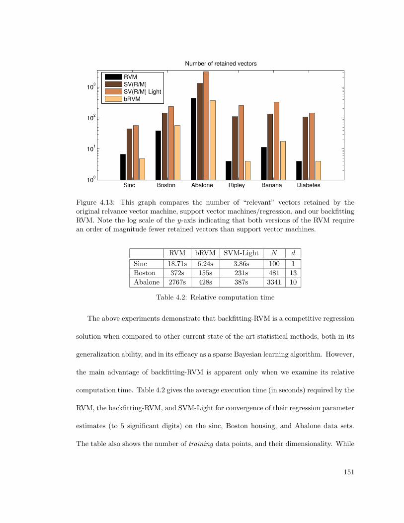
Sinc Boston Abalone Ripley Banana Diabetes100

101

102

103

Number of retained vectors

RVMSV(R/M)SV(R/M) LightbRVM

Figure 4.13: This graph compares the number of “relevant” vectors retained by theoriginal relvance vector machine, support vector machines/regression, and our backfittingRVM. Note the log scale of the y-axis indicating that both versions of the RVM requirean order of magnitude fewer retained vectors than support vector machines.

RVM bRVM SVM-Light N d

Sinc 18.71s 6.24s 3.86s 100 1

Boston 372s 155s 231s 481 13

Abalone 2767s 428s 387s 3341 10

Table 4.2: Relative computation time

The above experiments demonstrate that backfitting-RVM is a competitive regression

solution when compared to other current state-of-the-art statistical methods, both in its

generalization ability, and in its efficacy as a sparse Bayesian learning algorithm. However,

the main advantage of backfitting-RVM is apparent only when we examine its relative

computation time. Table 4.2 gives the average execution time (in seconds) required by the

RVM, the backfitting-RVM, and SVM-Light for convergence of their regression parameter

estimates (to 5 significant digits) on the sinc, Boston housing, and Abalone data sets.

The table also shows the number of training data points, and their dimensionality. While

151

SVM-Light does better than the backfitting-RVM, we note that it retains significantly

more basis vectors in the final solution. In spite of this, backfitting-RVM is within the

same order of magnitude in computation time. Note that the number of O(N 2) updates

to b per update cycle of the hyperparameters is very small (∼ 10), since the solution

from the previous update cycle is a very good starting point for the iterations of the next

cycle. The results demonstrate that the backfitting-RVM can significantly gain from the

iterative nature of the Bayesian backfitting generalized linear regression procedure.

152

Chapter 5

Conclusion

In the drive towards greater autonomy in intelligent systems, this dissertation contributes

theory and algorithms that seek to automate the model creation process by providing

a framework within which statistical model complexity is automatically derived in a

tractable and efficient manner. We tackled several particularly difficult problems of model

complexity estimation, for which to date, there have been no clear solutions which allow

general applicability in real-world applications.

5.1 Summary of Dissertation Contributions

In chapter 2 we reviewed inference in graphical models and derived the factorial variational

approximation as an extension to the popular EM algorithm. The factorial variational

approximation is related to the mean-field approximation which has been widely used

in statistical physics, and also has an interpretation as a message-passing or propagation

algorithm (Ghahramani & Beal 2001) similar to the junction tree method. The key as-

sumption is one of factorization in the posterior distribution over the unknown variables

in the model. When applied to graphical models which have conditional distributions

153

within the conjugate-exponential family, one can derive update equations for the poste-

rior distributions over the hidden variables which are analytically tractable, and which

ensure a monotonic decrease of the KL divergence between the true joint posterior and

its factorial approximation. Non-conjugate distributions can be handled by deriving ad-

ditional bounds using the theory of convex duality (Wainwright & Jordan 2003). This

formulation formed the basis for the analytical update equations for models presented in

later chapters.

Chapter 3 introduced three novel analytical solutions to difficult model complexity

estimation problems. The first deals with the problem of estimating the complexity of

mixture models. We put forward the idea that the decision to grow model complexity can

be made efficiently by examining local decisions on whether to split existing components.

This reduces the problem to deriving a principled splitting criterion, for which we look at

the marginal likelihood comparison between the existing component, and a hypothetical

model which splits the component in two. A factorial variational approximation to the

marginal likelihood gives us analytically tractable update equations, such that maximiz-

ing the marginal likelihood automatically chooses the hypothesis that best models the

data. We demonstrated the efficacy of this procedure by analyzing a data set consisting

of human movement data, in order to determine the dimensionality of the underlying

manifold.

The second algorithm presented in chapter 3 dealt with the problem of estimating

the extent of the window of sufficient statistics that should be cached in online learning

scenarios. This is also a model complexity problem since a very small window can explain

larger parameter drifts in the model and hence more complex data sets. Getting this

154

complexity parameter right is crucial since having a window that is too large will respond

only sluggisly to rapid parameter changes, while having one that is too small will respond

to noise fluctuations and fail to generalize well. We suggest a solution that is based

on tracking the parameters of a drifting system using a Kalman filter. By using the

anti-causal information available (Kalman smoothing), we can create a formulation for

estimating the process noise variance, which relates to how quickly we believe the system

changes with time. We show that in conjunction with the Bayesian backfitting algorithm

presented in chapter 4, we can provide a principled online learning algorithm that has no

open parameters to tune, and yet tracks the drifting process well.

Our final exploration of analytical tractability tackled the problem of estimating dis-

tance metrics for locally weighted learning — a problem also known as supersmoothing.

This proves to be a particularly difficult problem in practice, since unlike the standard

probabilistic formulations like mixture-of-experts, we would like the individual compo-

nents to be non-competitive, in order to provide for a computationally efficient solution.

This goal is accomplished by treating the kernel weights probabilistically, which also leads

to interesting design questions about the kernel form such that analytical tractability is

retained. By using a bound derived from the theory of convex duality, we created a simple

and efficient procedure for estimating the width of the kernel, such that it adapts locally

to the data without overfitting or underfitting.

Our main contribution to computationally efficient algorithms was provided in chap-

ter 4, in which we examined the family of backfitting algorithms as a candidate for reduc-

ing the computational complexity of supervised learning problems by decomposing infer-

ence along individual features. Several efficient procedures such as cascade-correlation

155

neural networks, and generalized Gauss-Seidel procedures can be shown to have algorith-

mic underpinnings that stem from the backfitting family of algorithms. Unfortunately,

until now, backfitting has been ignored by the larger machine learning community since

it does not have a probabilistic description. We therefore proposed the first probabilistic

derivation of this family of algorithms that stems from the EM optimization procedure,

and thus provides a natural analysis of its convergence properties. Moreover, given its

probabilistic derivation, we can extend the algorithm to incorporate more sophisticated

Bayesian inference such as automatic relevance detection.

The key advantage of Bayesian backfitting is its numerical robustness, since it re-

quires no matrix inversion. Empirically this also results in a computational saving since

updates to the distributions over the hyperparameters of the model do not require an

expensive matrix inversion step to recompute regression coefficients. Each EM step has

linear computational complexity in the number of dimensions d which results in an algo-

rithm which scales easily to high dimensional data sets. Extensions to classification and

categorical outputs is easily achieved using bounds derived from the principle of convex

duality. Another interesting consequence of the probabilistic derivation of backfitting is

that the framework of sparse Bayesian learning, and in particular, the relevance vector

machine can be derived with Bayesian backfitting at its core, thus allowing us to vastly

improve on its robustness and computational scalability.

156

5.2 Opportunities for Further Research

While we hope that the algorithms presented in this dissertation are widely applicable

over a large range of data sets, they are not the last word on their respective topics.

The variational approximation techniques described in this dissertation all have their

roots in the theory of convex duality, allowing the derivation of several families of approxi-

mations including the factorial variational approximation, Bethe/Kikuchi approximations

and cluster variation techniques. While there exists some analysis of the free-energy be-

haviour of these approximations (Wainwright & Jordan 2003), there is still no clear inter-

pretaton of the implications each variant has on the outcome of the statistical analysis.

MacKay (2001) suggests an interesting interpretation of the update equations that result

from the variational analysis, and shows that when interpreted as a system of discrete-

time dynamical equations, the interaction between the observed data and the structure of

the conditional distributions can be interpreted as phase-transitions which move between

models of varying complexity. The exploration of these ideas and their relation to the

outcome of statistical analysis would be a topic of interesting further research.

The extension of Bayesian backfitting to classification, and the Bayesian supersmooth-

ing algorithm both used a functional variational approximation in addition to the bound

from the factorial approximation. Part of the criticism of variational methods that use

functional rather than factorial bounds, is that the choice of the appropriate transfor-

mation (and hence the family of lower bound functions) seems to be more of an art

than an established procedure. Also, unlike the factorial approximation in which we can

cleanly quantify the tightness of the bound in terms of a KL divergence, there is no such

157

analysis for more general functional bounds. As we noted in our derivation of Bayesian

supersmoothing in section 3.3, when working outside the conjugate-exponential family,

we often need to make these additional functional variational approximations, and an au-

tomated procedure for deriving tight bounds is still elusive. The software system VIBES

(Variational Inference for Bayesian Networks) (Winn, Spiegelhalter & Bishop 2003) is

a popular tool for performing automated variational inference in Bayesian networks of

directed and undirected graphical models. While it can handle creating the appropriate

factorization in models which fall within the conjugate-exponential family, it cannot yet

handle the more general case of models that do not.

While our growing mixture model formulation works well in practice, it still suffers

from the curse of dimensionality when used in problems with more than a few hundred

dimensions. This primarily stems from the modeling of Wishart distributions over the

local covariance matrices of the mixture components. At present, the only viable solution

for very high-dimensional data seems to be to use local models which are axis-aligned,

thus reducing the problem to modeling only the diagonal elements of the covariance ma-

trices, which can be achieved easily with inverse Gamma distributions over each diagonal

component.

Our formulation of Bayesian forgetting factors tackles the problem of learning how

quickly to forget past data in online environments. It still however has the unfortunate

need to rely on a smoothing pass to correct an overestimate in the rate of process drift.

While we can reliably detect the window size of the Bayes filter in such situations, it

would be desirable if we could cache and recursively update sufficient statistics, instead

of keeping past data around for the duration of the window.

158

As we mentioned in section 3.1.4, the use of semiparametric Bayesian methods for

mixture modeling growing within the machine learning community, and it would be in-

teresting to interpret several efficient learning algorithms such as locally weighted projec-

tion regression (LWPR) within this framework. At the moment its dependence on Gibbs

sampling restricts its application to relatively low-dimensional densities, but this should

not prove to be a problem when adapting to methods like LWPR and backfitting since

they decompose multivariate problems in to series of univariate ones, within which the

semiparametric approach would still be efficient. It would also be interesting to see if

this can be combined with the variational approach to deal with density functions that

do not conform to the conjugate-exponential family.

159

Reference List

Akaike, H. (1974), ‘A new look at the statistical model identification’, IEEE Transactionson Automatic Control 19, 716–723.

Andrieu, C., de Freitas, N., Doucet, A. & Jordan, M. I. (2003), ‘An introduction toMCMC for machine learning’, Journal of Machine Learning Research 50, 5–43.

Antoniak, C. E. (1974), ‘Mixtures of Dirichlet processes with applications to Bayesiannonparametric problems’, The Annals of Statistics 2(6), 1152–1174.

Atkeson, C. G., Moore, A. W. & Schaal, S. (1997), ‘Locally weighted learning’, ArtificialIntelligence Review 11(1-5), 11–73.

Beal, M. J. (2003), Variational Algorithms for Approximate Bayesian Inference, PhDthesis, The Gatsby Computational Neurosience Unit, University College London, 17Queen Square, London WC1N 3AR.

Beal, M. J., Ghahramani, Z. & Rasmussen, C. E. (2002), The infinite hidden markovmodel, in Dietterich, Becker & Ghahramani (2002).

Becker, S., Thrun, S. & Obermayer, K., eds (2003), Advances in Neural InformationProcessing Systems 15, Vol. 15, MIT Press, Cambridge, MA.

Belsley, D. A., Kuh, E. & Welsch, R. E. (1980), Regression diagnostics: Identifyinginfluential data and sources of collinearity, Wiley, New York.

Bernardo, J. M. & Smith, A. F. M. (1994), Bayesian Theory, John Wiley & Sons, Inc.

Bishop, C. M. (1995), Neural Networks for Pattern Recognition, Oxford University Press.

Bishop, C. M. (1999a), Bayesian PCA, in M. S. Kearns, S. A. Solla & D. A. Cohn,eds, ‘Advances in Neural Information Processing Systems 11’, Vol. 11, MIT Press,Cambridge, MA, pp. 382–388.

Bishop, C. M. (1999b), Variational principle components, in ‘Proceedings of the Interna-tional Conference on Artificial Neural Networks (ICANN’99)’, IEE Press, Edinburgh,pp. 509–514.

Bishop, C. M. & Winn, J. M. (2000), Non-linear Bayesian image modelling, in D. Vernon,ed., ‘Proceedings of the 6th European Conference on Computer Vision’, Vol. 1842of Lecture Notes in Computer Science, Springer-Verlag.

160

Blackwell, D. (1973), ‘Discreteness of Ferguson selections’, The Annals of Statistics1(2), 356–358.

Blackwell, D. & MacQueen, J. B. (1973), ‘Ferguson distributions via Polya urn schemes’,The Annals of Statistics 1(2), 353–355.

Blei, D. M. & Jordan, M. I. (2004), Variational methods for the dirichlet process, in‘Proceedings of the 21st International Conference on Machine Learning’.

Cadez, I. V. & Smyth, P. (2001), Model complexity, goodness of fit, and diminishingreturns, in T. Leen, T. Dietterich & V. Tresp, eds, ‘Advances in Neural InformationProcessing Systems’, Vol. 13, MIT Press, pp. 388–394.

Chuang, R. & Mendell, N. R. (1997), ‘The approximate null distribution of the likelihoodratio test for a mixture of two bivariate normal distributions with equal variance’,Communications in Statistics — Simulation and Computation 26, 631–648.

Chun, F., Handjani, S. & Jungreis, D. (2003), ‘Generalizations of Polya’s urn problem’,Annals of Combinatorics 7(2), 141–154.

de Freitas, J. F. G., Niranjan, M. & Gee, A. H. (1999), Regularization in sequential learn-ing algorithms, in ‘Advances in Neural Information Processing Systems’, Vol. 10,MIT Press, pp. 458–464.

Dempster, A. P., Laird, N. M. & Rubin, D. B. (1977), ‘Maximum likelihood from incom-plete data via the EM algorithm’, Journal of the Royal Statistical Society. Series B(Methodological) 39(1), 1–38.

Deutscher, J., Blake, A. & Reid, I. (2000), Articulated body motion capture by annealedparticle filtering, in ‘Proceedings of the IEEE Conference on Computer Vision andPattern Recognition’, Vol. 2, pp. 126–133.

Dietterich, T., Becker, S. & Ghahramani, Z., eds (2002), Advances in Neural InformationProcessing Systems 14, Vol. 14, MIT Press, Cambridge, MA.

Doucet, A., de Freitas, N. & Gordon, N. J., eds (2001), Sequential Monte Carlo Methodsin Practice, Statistics for Engineering and Information Science, Springer-Verlag, NewYork.

D’Souza, A., Vijayakumar, S. & Schaal, S. (2001), Are internal models of the entire bodylearnable?, in ‘Society for Neuroscience Abstracts’, Vol. 27. Program No. 406.2.

D’Souza, A., Vijayakumar, S. & Schaal, S. (2004), The Bayesian backfitting relevancevector machine, in ‘Proceedings of the 21st International Conference on MachineLearning’, ACM Press.

Escobar, M. D. (1994), ‘Estimating normal means with a Dirichlet process prior’, Journalof the American Statistical Association 89(425), 268–277.

Escobar, M. D. & West, M. (1995), ‘Bayesian density estimation and inference usingmixtures’, Journal of the American Statistical Association 90(430), 577–588.

161

Everitt, B. S. (1984), An Introduction to Latent Variable Models, Monographs on Statis-tics and Applied Probability, Chapman & Hall.

Fahlman, S. E. & Lebiere, C. (1990), The cascade-correlation learning architecture, inD. S. Touretzky, ed., ‘Advances in Neural Information Processing Systems 2’, Vol. 2,Morgan Kaufmann Publishers.

Fearnhead, P. (1998), Sequential Monte Carlo methods in filter theory, PhD thesis, Mer-ton College, University of Oxford.

Feder, M. & Weinstein, E. (1988), ‘Parameter estimation of superimposed signals usingthe EM algorithm’, IEEE Transactions on Acoustics, Speech and Signal Processing36(4), 477–490.

Ferguson, T. S. (1973), ‘A Bayesian analysis of some nonparametric problems’, The An-nals of Statistics 1(2), 209–230.

Ferguson, T. S. (1974), ‘Prior distributions on spaces of probability measures’, The Annalsof Statistics 2(4), 615–629.

Frank, I. E. & Friedman, J. H. (1993), ‘A statistical view of some chemometrics regressiontools’, Technometrics 35(2), 109–135.

Friedman, J. H. (1984), A variable span smoother, Technical Report LCS5, Departmentof Statistics, Stanford University.

Friedman, J. H., Bentley, J. L. & Finkel, R. A. (1977), An algorithm for finding bestmatches in logarithmic expected time, in ‘ACM Transactions on Mathematical Soft-ware’, Vol. 3, pp. 209–226.

Fukumizu, K., Bach, F. R. & Jordan, M. I. (2004), ‘Dimensionality reduction for super-vised learning using reproducing kernel Hilbert spaces’, Journal of Machine LearningResearch 5, 73–99.

Gelman, A., Carlin, J. B., Stern, H. S. & Rubin, D. B. (1995), Bayesian Data Analysis,Texts in Statistical Science, Chapman & Hall/CRC, Boca Raton, Florida.

Geman, S., Bienestock, E. & Doursal, R. (1992), ‘Neural networks and the bias/variancedilemma’, Neural Computation 4, 1–58.

Geman, S. & Geman, D. (1984), ‘Stochastic relaxation, Gibbs distributions and theBayesian restoration of images’, IEEE Transactions on Pattern Analysis and Ma-chine Intelligence 6, 721–741.

Ghahramani, Z. & Beal, M. J. (2000), Variational inference for Bayesian mixtures offactor analysers, in Solla, Leen & Muller (2000), pp. 509–514.

Ghahramani, Z. & Beal, M. J. (2001), Propagation algorithms for variational Bayesianlearning, in Leen, Diettrich & Tresp (2001).

162

Ghahramani, Z. & Hinton, G. E. (1997), The EM algorithm for mixtures of factor analyz-ers, Technical Report CRG-TR-96-1, Department of Computer Science, Universityof Toronto, 6 King’s College Road, Toronto, Canada M5S 1A4.

Ghosh, J. K. & Ramamoorthi, R. V. (2003), Bayesian Nonparametrics, Springer Seriesin Statistics, Springer-Verlag, New York, USA, chapter Dirichlet and Polya TreeProcesses, pp. 87–120.

Gordon, N. J., Salmond, D. J. & Smith, A. F. M. (1993), ‘Novel approach tononlinear/non-Gaussian Bayesian state estimation’, IEE Proceedings-F 140(2), 107–113.

Gray, A. & Moore, A. W. (2001), N -body problems in statistical learning, in Leen et al.(2001).

Green, P. J. (1995), ‘Reversible jump Markov chain Monte Carlo computation andBayesian model determination’, Biometrika 82, 711–732.

Hammersley, J. M. & Clifford, P. (1971), Markov fields on finite graphs and lattices.Unpublished.

Hastie, T. J. & Tibshirani, R. J. (1990), Generalized Additive Models, number 43 in‘Monographs on Statistics and Applied Probability’, Chapman & Hall.

Hastie, T. J. & Tibshirani, R. J. (2000), ‘Bayesian backfitting’, Statistical Science15(3), 196–213.

Hastie, T. J., Tibshirani, R. J. & Friedman, J. H. (2001), The Elements of Statisti-cal Learning: Data Mining, Inference, and Prediction, Springer Series in Statistics,Springer-Verlag.

Hastings, W. K. (1970), ‘Monte Carlo sampling methods using Markov chains and theirapplications’, Biometrika 57, 97–109.

Hurvich, C. & Tsai, C. (1976), ‘Regression and time series model selection in smallsamples’, Biometrika 76, 297–307.

Ishwaran, H. & James, L. F. (2001), ‘Gibbs sampling methods for stick-breaking priors’,Journal of the American Statistical Association 96(453), 161–173.

Ishwaran, H. & James, L. F. (2002), ‘Approximate Dirichlet process computing in finitenormal mixtures: Smoothing and prior information’, Journal of Computational andGraphical Statistics 11(3), 1–26.

Ishwaran, H. & Zarepour, M. (2002), ‘Exact and approximate sum-representations forthe Dirichlet process’, Canadian Journal of Statistics 30, 269–283.

Jaakkola, T. S. & Jordan, M. I. (2000), ‘Bayesian parameter estimation via variationalmethods’, Statistics and Computing 10(1), 25–37.

163

Jeffreys, H. (1946), ‘An invariant form for the prior probability in estimation problems’,Journal of the Royal Statistical Society. Series A 186, 453–461.

Jordan, M. I., Ghahramani, Z., Jaakkola, T. S. & Saul, L. K. (1999), An introduction tovariational methods for graphical models, in M. I. Jordan, ed., ‘Learning in GraphicalModels’, MIT Press, pp. 105–161.

Jordan, M. I. & Jacobs, R. A. (1994), ‘Hierarchical mixtures of experts and the EMalgorithm’, Neural Computation 6(2), 181–214.

Kalman, R. E. (1960), ‘A new approach to linear filtering and prediction problems’,Transactions of the ASME — Journal of Basic Engineering 82, 35–45.

Kawato, M. (1999), ‘Internal models for motor control and trajectory planning’, CurrentOpinion in Neurobiology 9, 718–727.

Komarek, P. & Moore, A. W. (2000), A dynamic adaptation of AD-trees for efficientmachine learning on large data sets, in P. Langley, ed., ‘International Conference onMachine Learning’, pp. 495–502.

Lauritzen, S. L. (1996), Graphical Models, Vol. 17 of Oxford Statistical Science Series,Oxford Science Publications.

Lauritzen, S. L. & Spiegelhalter, D. J. (1988), ‘Local computations with probabilitieson graphical structures and their applications to expert systems (with discussion)’,Journal of the Royal Statistical Society. Series B (Methodological) 50(2), 157–224.

Leen, T. K., Diettrich, T. G. & Tresp, V., eds (2001), Advances in Neural InformationProcessing Systems 13, Vol. 13, MIT Press, Cambridge, MA.

Li, J. Q. & Barron, A. R. (2001), Mixture density estimation, in Leen et al. (2001),pp. 279–285.

Ljung, L. & Soderstrom, T. (1983), Theory and Practice of Recursive Identification, MITPress, Cambridge, Massachusets.

MacEachern, S. N. & Muller, P. (1998), ‘Estimating mixture of Dirichlet process models’,Journal of Computational and Graphical Statistics 7, 223–238.

MacKay, D. J. C. (1999), ‘Comparison of approximate methods for handling hyperpa-rameters’, Neural Computation 11(5), 1035–1068.

MacKay, D. J. C. (2001), Local minima, symmetry breaking, and model pruning invariational free energy minimization. Unpublished.

MacKay, D. J. C. (2003a), Information Theory, Inference and Learning Algorithms, Cam-bridge University Press, chapter Monte Carlo Methods, pp. 357–386.

MacKay, D. J. C. (2003b), Information Theory, Inference and Learning Algorithms, Cam-bridge University Press, chapter Variational Methods, pp. 422–436.

164

Massey, W. F. (1965), ‘Principal component regression in exploratory statistical research’,Journal of the American Statistical Association 60, 234–246.

McLachlan, G. & Peel, D. (2000), Finite Mixture Models, Wiley series in probability andstatistics, John Wiley & Sons, Inc., New York, NY.

Mendell, N. R., Finch, S. J. & Thode, H. C. (1993), ‘Where is the likelihood ratio testpowerful for detecting two component mixtures?’, Biometrics 49, 907–915.

Mengerson, K. & Robert, C. P. (1996), Testing for mixtures: A Bayesian entropy ap-proach, in J. O. Berger, J. M. Bernardo, A. P. Dawid, D. V. Lindley & A. F. M.Smith, eds, ‘Bayesian Statistics’, Vol. 5, Oxford University Press.

Metropolis, N., Rosenbluth, A. W., Rosenbluth, M. N., Teller, A. H. & Teller, E. (1953),‘Equation of state calculations by fast computing machines’, Journal of ChemicalPhysics 21, 1087–1092.

Minagawa, A., Tagawa, N. & Tanaka, T. (2002), ‘SMEM algorithm is not fully compatiblewith maximum likelihood framework’, Neural Computation 14, 1261–1266.

Mitchell, T. M. (1997), Machine Learning, WCB/McGraw Hill.

Moore, A. W. (2000), The anchors hierarchy: Using the triangle inequality to survivehigh-dimensional data, in ‘Proceedings of the Twelfth International Conference onUncertainty in Artificial Intelligence’, AAAI Press, pp. 397–405.

Moore, A. W. & Lee, M. S. (1998), ‘Cached sufficient statistics for efficient machinelearning with large datasets’, Journal of Artificial Intelligence Research 8, 67–91.

Motwani, R. & Raghavan, P. (1995), Randomized Algorithms, Cambridge UniversityPress.

Neal, R. M. (1994), Bayesian Learning for Neural Networks, PhD thesis, Dept. of Com-puter Science, University of Toronto.

Neal, R. M. (1998), Markov chain sampling methods for Dirichlet process mixture models,Technical Report 9815, Department of Statistics, University of Toronto, Toronto,Canada.

Neal, R. M. & Hinton, G. E. (1998), A view of the EM algorithm that justifies incremental,sparse, and other variants, in M. I. Jordan, ed., ‘Learning in Graphical Models’,Kluwer Academic Publishers, Dordecht, The Netherlands, pp. 355–368.

Omohundro, S. M. (1991), Bumptrees for efficient function, constraint and classificationlearning, in R. Lippmann, J. Moody & D. S. Touretzky, eds, ‘Advances in NeuralInformation Processing Systems 3’, Vol. 3, Morgan Kaufmann Publishers, pp. 693–699.

Paciorek, C. J. & Schervish, M. J. (2004), Nonstationary covariance functions for Gaus-sian process regression, in Thrun, Saul & Scholkopf (2004).

165

Parisi, G. (1988), Statistical Field Theory, Vol. 66 of Frontiers in Physics, Addison-Wesley,Redwood City, CA.

Pearl, J. (1988), Probabilistic Reasoning in Intelligent Systems: Networks of PlausibleInference, Morgan Kaufmann Publishers.

Pitman, J. & Yor, M. (1997), ‘The two-parameter Poisson-Dirichlet distribution derivedfrom a stable subordinator’, The Annals of Statistics 25(2), 855–900.

Poggio, R. & Girosi, F. (1990), ‘Regularization algorithms for learning that are equivalentto multilayer networks’, Science 247, 213–225.

Proakis, J. G., Rader, C. M., Ling, F., Nikias, C. L., Moonen, M. & Proudler, I. K. (2002),Algorithms for Statistical Signal Processing, Prentice Hall, Upper Saddle River, NewJersey.

Rasmussen, C. E. (2000), The infinite Gaussian mixture model, in Solla et al. (2000),pp. 554–560.

Rasmussen, C. E. & Ghahramani, Z. (2002), Infinite mixtures of gaussian process experts,in Dietterich et al. (2002).

Ratsch, G., Onoda, T. & Muller, K.-R. (2001), ‘Soft margins for AdaBoost’, MachineLearning 42(3), 287–320.

Richardson, S. & Green, P. J. (1997), ‘On Bayesian analysis of mixtures with an un-known number of components’, Journal of the Royal Statistical Society. Series B(Methodological) 59, 731–792.

Rissanen, J. (1978), ‘Modelling by shortest data description’, Automatica 14, 465–471.

Rissanen, J. (1996), ‘Fisher information and stochastic complexity’, IEEE Transactionson Information Theory 42(1), 40–47.

Roeder, K. & Wasserman, L. (1995), Practical Bayesian density estimation using mix-tures of normals, Technical Report 633, Department of Statistics, Carnegie MellonUniversity.

Rubin, D. B. (1988), Using the SIR algorithm to simulate posterior distributions, inJ. Bernado, M. H. DeGroot, D. V. Lindley & A. F. M. Smith, eds, ‘Bayesian Statistics3’, Oxford University Press, pp. 395–403.

Rustagi, J. S. (1976), Variational Methods in Statistics, Vol. 121 of Mathematics in Sci-ence and Engineering, Academic Press, New York.

Sato, M. (2001), ‘Online model selection based on the variational Bayes’, Neural Compu-tation 13(7), 1649–1681.

Saul, L. K., Jaakkola, T. S. & Jordan, M. I. (1996), ‘Mean field theory for sigmoid beliefnetworks’, Journal of Artificial Intelligence Research 4, 61–76.

166

Schaal, S. & Atkeson, C. G. (1998), ‘Constructive incremental learning from only localinformation’, Neural Computation 10, 2047–2084.

Schaal, S. & Sternad, D. (2001), ‘Origins and violations of the 2/3 power law in rhythmic3d movements’, Experimental Brain Research 136, 60.

Schaal, S., Vijayakumar, S. & Atkeson, C. G. (1998), Local dimensionality reduction,in M. I. Jordan, M. S. Kearns & S. A. Solla, eds, ‘Advances in Neural InformationProcessing Systems 10’, Vol. 10, MIT Press, Cambridge, MA, pp. 633–639.

Scholkopf, B. & Smola, A. J. (2000), Learning with Kernels — Support Vector Machines,Regularization, Optimization, and Beyond, Adaptive Computation and MachineLearning, MIT Press.

Schwarz, G. (1978), ‘Estimation the dimension of a model’, The Annals of Statistics6, 461–464.

Sethuraman, J. (1994), ‘A constructive definition of Dirichlet priors’, Statistica Sinica4, 639–650.

Smyth, P. (2000), ‘Model selection for probabilistic clustering using cross validated like-lihood’, Statistics and Computing 10, 63–72.

Solla, S. A., Leen, T. K. & Muller, K.-R., eds (2000), Advances in Neural InformationProcessing Systems 12, Vol. 12, MIT Press, Cambridge, MA.

Stone, M. (1974), ‘Cross-validatory choice and assessment of statistical predictions’, Jour-nal of the Royal Statistical Society. Series B (Methodological) 36(1), 111–147.

Stone, M. & Brooks, R. J. (1990), ‘Continuum regression: Cross-validated sequentiallyconstructed prediction embracing ordinary least squares, partial least squares andprincipal components regression’, Journal of the Royal Statistical Society. Series B(Methodological) 52(2), 237–269.

Sykacek, P. & Roberts, S. J. (2003), Adaptive classification by variational Kalman filter-ing, in Becker, Thrun & Obermayer (2003), pp. 737–744.

Thrun, S. (2002), Particle filters in robotics, in ‘Proceedings of the International Confer-ence on Uncertainty in Artificial Intelligence (UAI 2002)’.

Thrun, S., Saul, L. K. & Scholkopf, B., eds (2004), Advances in Neural InformationProcessing Systems 16, Vol. 16, MIT Press, Cambridge, MA.

Tipping, M. E. (2000), The relevance vector machine, in Solla et al. (2000).

Tipping, M. E. (2001), ‘Sparse Bayesian learning and the relevance vector machine’,Journal of Machine Learning Research 1, 211–244.

Tipping, M. E. & Bishop, C. M. (1999), ‘Mixtures of probabilistic principal componentanalysers’, Neural Computation 11(2), 443–482.

167

Tipping, M. E. & Faul, A. C. (2003), Fast marginal likelihood maximization for sparseBayesian models, in C. M. Bishop & B. J. Frey, eds, ‘Proceedings of the NinthInternational Workshop on Artificial Intelligence and Statistics’.

Ueda, N. & Nakano, R. (1998), ‘Deterministic annealing EM algorithm’, Neural Networks11, 271–282.

Ueda, N., Nakano, R., Ghahramani, Z. & Hinton, G. E. (1999), SMEM algorithm formixture models, in M. S. Kearns, S. A. Solla & D. A. Cohn, eds, ‘Advances inNeural Information Processing Systems’, Vol. 11, MIT Press.

Vapnik, V. N. (1982), Estimation of Dependences Based on Empirical Data, Springer-Verlag, Berlin.

Vapnik, V. N. (1995), The Nature of Statistical Learning Theory, Springer-Verlag, NewYork.

Vermaak, J., Godsill, S. J. & Doucet, A. (2004), Sequential Bayesian kernel regression,in Thrun et al. (2004).

Vijayakumar, S., D’Souza, A. & Schaal, S. (2004), ‘Incremental online learning in highdimensions’, Neural Computation . (submitted).

Vijayakumar, S., D’Souza, A., Shibata, T., Conradt, J. & Schaal, S. (2000), ‘Statisticallearning for humanoid robots’, Autonomous Robots 12, 55–69.

Vijayakumar, S. & Schaal, S. (2000), An O(n) algorithm for incremental real time learningin high dimensional space, in ‘Proceedings of the Seventeenth International Confer-ence on Machine Learning (ICML2000)’, Stanford, CA, pp. 1079–1086.

Wainwright, M. J. & Jordan, M. I. (2003), Graphical models, exponential families, andvariational inference, Technical Report 649, Department of Statistics, University ofCalifornia, Berkeley.

Williams, C. K. I. (1997), Prediction with Gaussian processes: From linear regressionto linear prediction and beyond, Technical Report NCRG/97/012, Neural Comput-ing Research Group, Dept. of Computer Science & Applied Mathematics, AstonUniversity, Birmingham B4 7ET, United Kingdom.

Williams, C. K. I. & Rasmussen, C. E. (1996), Gaussian processes for regression, in D. S.Touretzky, M. C. Mozer & M. E. Hasselmo, eds, ‘Advances in Neural InformationProcessing Systems 8’, Vol. 8, MIT Press, Cambridge, MA, pp. 514–520.

Winn, J. M., Spiegelhalter, D. J. & Bishop, C. M. (2003), VIBES: A variational inferenceengine for Bayesian networks, in Becker et al. (2003), pp. 793–800.

Wold, H. (1975), Soft modeling by latent variables: The nonlinear iterative partial leastsquares approach, in J. Gani, ed., ‘Perspectives in Probability and Statistics, Papersin Honour of M. S. Bartlett’, Academic Press, London, pp. 520–540.

168

Wu, C. F. J. (1983), ‘On the convergence properties of the EM algorithm’, The Annalsof Statistics 11(1), 95–103.

Zhang, Y.-J. & Liu, Z.-Q. (2002), ‘Self-splitting competitive learning: A new on-lineclustering paradigm’, IEEE Transactions on Neural Networks 13(2), 369–380.

169

Appendix A

Some Useful Results

A.1 Schur Complements

If we partition M =

[A BC D

]then we can write the following Schur complements:

MA = D−CA−1B

MD = A−BD−1C

−MB = C−DB−1A if B−1 exists

−MC = B−AC−1D if C−1 exists

This allows us to express the inverse of M as follows:

M−1 =

[M−1

D −M−1B

−M−1C M−1

A

]

Importantly if B and C are singular, then we can obtain M−1B and M−1

D in terms ofbenign inversions by using the property that MM−1 = I and M−1M = I to realize:

CM−1D = DM−1

C

M−1B D = M−1

D B

These results prove highly useful when computing partial matrix inversions, such asthose required when conditioning multivariate Gaussian distributions.

170

A.2 Some Important Expectations

Frequently we are required to compute the expectation 〈lnx〉 where x is distributedaccording to a Beta (conjugate for Binomial probability), Dirichlet (conjugate for Multi-nomial probability vector), Gamma (conjugate for Gaussian precision), or Wishart (con-jugate for multivariate Gaussian precision). These are frequently expressed in terms ofthe digamma function:

ψ(a) =d ln Γ(x)

dx

∣∣∣∣x=a

where the Gamma function Γ(x) is an interpolant to the factorial defined as:

Γ(x) =

∫ ∞

0t(x−1) exp(−t)dt

for x > 0. For integer values of x, Γ(x) = (x− 1)!

• To compute 〈lnx〉 for x ∼ Beta (x; a, b) consider:

Beta (x; a, b) =Γ (a+ b)

Γ(a)Γ(b)xa−1 (1− x)b−1

=1

Zxa−1 (1− x)b−1

where:

Z =Γ(a)Γ(b)

Γ (a+ b)

=

∫ 1

0xa−1 (1− x)b−1 dx

Differentiating w.r.t. the parameter a we get:

d

daZ =

d

da

∫ 1

0xa−1 (1− x)b−1 dx

=

∫ 1

0(lnx)xa−1 (1− x)b−1 dx

= Z 〈lnx〉

Hence:

〈lnx〉 =1

Z

d

daZ

=d

dalnZ

171

=d

da(Γ(a) + Γ(b)− Γ(a+ b))

= ψ(a)− ψ(a+ b)

• The Dirichlet is a generalization of the beta distribution to a multinomial probabilityvector x:

Dirichlet (x; u) =Γ (∑

i ui)∏i Γ (ui)

∏

i

xui−1i

A property of the Dirichlet distribution is that each component xi is marginallydistributed as:

xi ∼ Beta

xi;ui,

∑

j 6=iuj

Thus the result above for the Beta distribution allows us to infer that:

〈lnxi〉 = ψ(ui)− ψ

∑

j

uj

• To compute 〈lnx〉 for x ∼ Gamma (x; a, b) consider:

Gamma (x; a, b) =ba

Γ(a)x(a−1) exp(−bx)

=1

Zx(a−1) exp(−bx)

where:

Z =Γ(a)

ba

=

∫ ∞

0x(a−1) exp(−bx)dx

Differentiating w.r.t. the parameter a we get:

d

daZ =

d

da

∫ ∞

0x(a−1) exp(−bx)dx

=

∫ ∞

0(lnx)x(a−1) exp(−bx)dx

= Z 〈lnx〉

Hence:

172

〈lnx〉 =1

Z

d

daZ

=d

dalnZ

=d

da

(ln Γ(a)− a ln b

)

= ψ (a)− ln b

• For a symmetric positive definite matrix X ∼ Wishartν (X; S) we often require〈ln |X|〉. Consider:

Wishartν (X; S) =|S|−ν/2

2νd/2πd(d−1)/4∏di Γ(ν+1−i

2

) |X|(ν−d−1)/2 exp

−1

2Tr[S−1X

]

=1

Z|X|(ν−d−1)/2 exp

−1

2Tr[S−1X

]

where:

Z =2νd/2πd(d−1)/4

∏di Γ(ν+1−i

2

)

|S|−ν/2

=

∫ ∞

O|X|(ν−d−1)/2 exp

−1

2Tr[S−1X

]dX

Differentiating w.r.t. the parameter ν we get:

d

dνZ =

d

dν

∫ ∞

O|X|(ν−d−1)/2 exp

−1

2Tr[S−1X

]dX

=

∫ ∞

O(ln |X|) |X|(ν−d−1)/2 exp

−1

2Tr[S−1X

]dX

= Z 〈ln |X|〉

Hence:

〈ln |X|〉 =1

Z

d

dνZ

=d

dνlnZ

=d

dν

(νd

2ln 2 +

d(d− 1)

4lnπ +

d∑

i

ln Γ

(ν + 1− i

2

)+ν

2ln |S|

)

173

=d∑

i

ψ

(ν + 1− i

2

)+d

2ln 2 +

1

2ln |S|

174

Appendix B

Derivations

B.1 Factorial Variational Approximation

Let us start with the lower bound derived in equation (2.4) of section 2.2.2. We know thatmaximizing the lower bound implies maximizing the functional F(Q,φ) over the spaceof probability distributions Q(xH). Let us consider a simple example in which xH =x1, x2, x3, and furthermore assume that Q(xH) factors over the individual variablesxi as Q(xH) = Q1(x1)Q2(x2)Q3(x3). The calculus of variations (see (Rustagi 1976)for example,) allows us to derive a very elegant and general update mechanism for theindividual factored distributions in our variational approximation.

For the ease of notation, in the rest of this derivation we shall use the symbol Qi todenote Qi(xi). Hence for our current example, the functional F (Q,φ) is of the form:

F (Q,φ) =

∫Q1Q2Q3 ln

p(xD,xH;φ)

Q1Q2Q3dx1dx2dx3 (B.1)

Maximizing F (Q,φ) is actually a constrained maximization since we must ensure that∫Q(xH)dxH = 1. This constraint can be incorporated into the integrand by the use of

Lagrange multipliers. We therefore define a new function z(xH) and derive a differentialconstraint as follows:

z(xH) =

∫ xH

−∞Q1(x′1)Q2(x′2)Q3(x′3)dx′1dx

′2dx′3

z −Q1Q2Q3 = 0 s.t. z(−∞) = 0 and z(∞) = 1 (B.2)

with the end point constraints being z(−∞) = 0 and z(∞) = 1. If we let g(Q1, Q2, Q3,xH)represent the integrand in equation (B.1), then we can incorporate the differential con-straint of equation (B.2) using the Lagrange multiplier λ as folows:

ga(Q1, Q2, Q3,xH, z, λ) = Q1Q2Q3 lnp(xD,xH;φ)

Q1Q2Q3+ λ(z −Q1Q2Q3) (B.3)

Using this constrained integrand, maximizing the functional F (Q,φ) w.r.t. each ofthe distributions Qi involves solving the following Euler equations:

175

∂ga∂Qi

− d

dxH

(∂ga

∂Qi

)= 0 (B.4)

∂ga∂z− d

dxH

(∂ga∂z

)= 0 (B.5)

where we denote Qi = dQi/dxH. Substituting from equation (B.3) in equation (B.5)we get dλ/dxH = 0. This implies that the Lagrange multiplier λ is not a function ofany of the hidden variables — an important result that will be used in the followingsteps. Similarly substituting from equation (B.3) in equation (B.4) and performing thedifferentiation with Qi = Q1 we get:

Q2Q3 [ln p(xD,xH;φ)− lnQ1 − lnQ2Q3]−Q2Q3 − λQ2Q3 = 0 (B.6)

Integrating the above equation w.r.t. x2 and x3 we get:

〈ln p(xD,xH;φ)〉Q2Q3− lnQ1 −

∫Q2Q3 lnQ2Q3dx2dx3 − 1− λ = 0 (B.7)

Solving for Q1 we get:

Q1 =exp 〈ln p(xD,xH;φ)〉Q2Q3

exp(1 + λ+

∫Q2Q3 lnQ2Q3dx2dx3

)

The denominator is independent of x1 since we have shown that λ is not a functionof the hidden variables, and our assumed independence Q(xH) = Q1(x1)Q2(x2)Q3(x3)implies that Q2Q3 is also independent of θ1. Hence the denominator can be treated assimply a normalizing constant, and we can express the solution for the individual Qi thatmaximizes the functional F (Q,φ) under the assumed factorization as:

Qi(xi) =exp 〈ln p(xD,xH;φ)〉Qk 6=i∫

exp 〈ln p(xD,xH;φ)〉Qk 6=i dxi

or equivalently:

lnQi(xi) = 〈ln p(xD,xH;φ)〉Qk 6=i + constxi

where 〈·〉Qk 6=i denotes expectation taken w.r.t. all distributions Qk except Qi.

B.1.1 Solution for Partial Factorization

Let us drop the assumption of complete factorization for now and examine how oursolution changes when the factorization is partial. Suppose our current example had thepartial factorization Q(xH) = Q12(x1, x2)Q3(x3) = Q1(x1|x2)Q2(x2)Q(x3), then if wewere trying to find a solution for Q1 we would not be able to separate the lnQ1 term out

176

of the integral as we have done in eq. (B.7), due to the fact that Q1 = Q1(x1|x2) and hasa dependency on x2. Our only way out of the problem is to infer the joint distributionQ12(x1, x2), and hope to be able to factor the resulting distribution into Q1(x1|x2)Q2(x2).

The final solution also changes if we were trying to maximize the functional w.r.t. Q2.We would proceed as if we assumed full factorization as before and arrive at the followingequation which is analogous to equation (B.7)

〈ln p(xD,xH;φ)〉Q1Q3− lnQ2 −

∫Q1Q3 lnQ1Q3dx1dx3 − 1− λ = 0

In this situation however, we must keep in mind that Q1 is actually Q1(x1|x2) andhence has a dependency on x2. Now when we solve for Q2 we should take care to placeall of the terms in the equation that have a dependency on x2 in the numerator. We thenarrive at the equation:

Q2(x2) ∝ exp

(〈ln p(xD,xH;φ)〉Q1Q3

−∫Q1(x1|x2) lnQ1(x1|x2)dx1

)

or equivalently

lnQ2 = 〈ln p(xD,xH;φ)〉Q1Q3+ entropy Q1(x1|x2)+ const

Note that this method gives exactly the same result as the equivalent method ofusing the simple factorial approximation to determine the update for the joint posteriorQ(x1, x2) and subsequently marginalizing out x1 to obtain Q(x2).

B.2 Variational Approximation for Mixture Models

For convenience, we will repeat the log probability of the of the statistical model repre-sented by figure 3.1:

ln p(xD,xH;M2) =N∑

i=1

si1

[1

2ln |P1| −

1

2(xi − µ1)TP1 (xi − µ1) + ln ζ

]

+ si2

[1

2ln |P2| −

1

2(xi − µ2)TP2 (xi − µ2) + ln (1− ζ)

]

+∑

m=1,2

[d

2lnα0 +

1

2ln |Pm| −

α0

2µm

TPmµm

]

+∑

m=1,2

[(ν − d− 1

2

)ln |Pm| −

1

2Tr[R−1Pm

]]

+ (u1 − 1) ln ζ + (u2 − 1) ln (1− ζ) + constxD,xH

(B.8)

177

If we assume the factorization Q(xH) = Q(µ,P)Q(S)Q(ζ), we can use the resultsderived in appendix B.1, to obtain the update equations for the marginal distributionsover each set of factored variables.

• For Q(ζ):

lnQ(ζ) =

(u1 +

N∑

i=1

〈si1〉 − 1

)ln ζ+

(u2 +

N∑

i=1

〈si2〉 − 1

)ln(1−ζ)+constζ (B.9)

From equation (B.9) we can infer the following:

Q(ζ) = Beta (ζ; u1, u2)

u1 = u1 +N∑

i=1

〈si1〉

u2 = u2 +N∑

i=1

〈si2〉

• For Q(µm,Pm):

lnQ(µm,Pm) =1

2

(N∑

i=1

〈sim〉)

ln |Pm| −1

2

N∑

i=1

〈sim〉 (xi − µm)TPm (xi − µm)

+1

2ln |Pm| −

α0

2µTmPmµm +

(ν − d− 1

2

)ln |Pm|

− 1

2Tr[S−1Pm

]+ constµm,Pm

(B.10)

From equation (B.10) we can infer the following:

Q(µm,Pm) = Normal(µm; m

(m)µ ,Σ

(m)µ

)Wishartνm

(Pm; Rm

)

xm =

∑Ni=1 〈sim〉xi∑Ni=1 〈sim〉

Σ(m)µ =

(N∑

i=1

〈sim〉+ α0

)−1

P−1m

m(m)µ = Σµm

(N∑

i=1

〈sim〉)

Pmxm =

∑Ni=1 〈sim〉∑N

i=1 〈sim〉+ α0

xm

178

R−1m = R−1 +

N∑

i=1

〈sim〉 (xi − xm) (xi − xm)T +

∑Ni=1 〈sim〉α0∑N

i=1 〈sim〉+ α0

xmxTm

νm = ν +N∑

i=1

〈sim〉

• For Q(S):

lnQ(si1 = 1) =1

2〈ln |P1|〉 −

1

2

⟨(xi − µ1)TP1 (xi − µ1)

⟩+ 〈ln ζ〉+ constsi1

Similarly,

lnQ(si2 = 1) =1

2〈ln |P2|〉 −

1

2

⟨(xi − µ2)TP2 (xi − µ2)

⟩+ 〈ln(1− ζ)〉+ constsi2

The expectation⟨

(xi − µm)TPm (xi − µm)⟩

is deceptively simple. Expanding the

quadratic as follows:

⟨(xi − µm)TPm (xi − µm)

⟩= xi

T 〈Pm〉xi − 2xTi 〈Pmµm〉+⟨µTmPµm

⟩

we notice that the only tricky expectations are 〈Pmµm〉 and⟨µTmPµm

⟩, which sim-

plify considerably on consideration of the update equations for Q(µm,Pm) giving:

⟨(xi − µm)TPm (xi − µm)

⟩=(xi − 〈µm|Pm〉

)T 〈Pm〉(xi − 〈µm|Pm〉

)

+ 〈Cov (µm|Pm) Pm〉

B.3 Variational Approximation for Forgetting Rates

For convenience, we will repeat the log probability of the of the statistical model repre-sented by figure 3.12:

ln p(y,w, λ, ψy|x) =N∑

n=1

[1

2lnψy2π− ψy

2(yn − wnxn)2

+1

2ln

λ

2π− λ

2(wn − wn−1)2

]

+1

2lnζ0

2π− ζ0

2(w0 − w0)2

+ aλ ln bλ − ln Γ (aλ) + (aλ − 1) lnλ− bλλ+ aψ ln bψ − ln Γ (aψ) + (aψ − 1) lnψy − bψψy

(B.11)

179

If we assume the factorization Q(xH) = Q(w)Q(λ, ψy), then from the graph structurein figure 3.12 we can see that this factorization also results in the factorization Q(λ, ψy) =Q(λ)Q(ψy). Hence, we can use the results derived in appendix B.1, to obtain the updateequations for the following marginal distributions:

• For Q(ψy):

lnQ(ψy) =N

2lnψy −

ψy2

N∑

n=1

⟨(yn − wnxn)2

⟩N

+ (aψ − 1) lnψy

− bψψy + constψy (B.12)

From equation (B.12) we can infer the following:

Q(ψy) = Gamma(ψy; aψ, bψ

)

aψ = aψ +N

2

bψ = bψ +1

2

N∑

n=1

⟨(yn − wnxn)2

⟩N

= bψ +1

2

N∑

n=1

[(yn − 〈wn〉N xn

)2+

1

ϕn

]

• For Q(λ):

lnQ(λ) =N

2lnλ− λ

2

N∑

n=1

⟨(wn − wn−1)2

⟩N

+ (aλ − 1) lnλ− bλλ+ constλ (B.13)

From equation (B.13) we can infer the following:

Q(λ) = Gamma(λ; aλ, bλ

)

aλ = aλ +N

2

bλ = bλ +1

2

N∑

n=1

⟨(wn − wn−1)2

⟩N

= bλ +1

2

N∑

n=1

[(〈wn〉N − 〈wn−1〉N

)2+

1

ϕn+

1

ϕn−1− 2 Cov (wn−1, wn)

]

In order to estimate the Cov (wn−1, wn) term we must consider the joint posteriordistribution of (wn−1, wn), which can be written as:

180

Q(wn−1, wn|xD1:N) =

Q (wn|wn−1)Q(wn−1|xD1:n−1

)∫Q (wn|wn−1)Q

(wn−1|xD1:n−1

)dwn−1

Q(wn|xD1:N)

where

Q (wn|wn−1) = Normal (wn;wn−1, 1/λ)

Q(wn−1|xD1:n−1

)= Normal

(wn−1; 〈wn−1〉n−1 , 1/ζn−1

)

Q(wn|xD1:N) = Normal (wn; 〈wn〉N , 1/ϕN )

Since all the distributions involved are Gaussian, it is easy to show that the resultingjoint distribution Q(wn−1, wn|xD1:N

) is also Gaussian, and using Schur complements(see appendix A.1), we can derive the off-diagonal covariance term:

Cov(wn−1, wn) =〈λ〉(ζn−1 + 〈λ〉

)

ϕn−1

[ϕn(ζn−1 + 〈λ〉

)+ 〈λ〉2

]

B.4 Derivation of Probabilistic Backfitting

To derive an EM solution to probabilistic backfitting, we begin with the complete loglikelihood of equation (4.15):

ln p(xD,xH;φ) = −N2

lnψy −1

2ψy

N∑

i=1

(yi − 1T zi

)2

−d∑

m=1

[N

2lnψzm +

1

2ψzm

N∑

i=1

(zim − bmfm(xi;θm)

)2]

+ const

Taking expectations w.r.t. p(xH|xD;φ) where xH = Z, and differentiating with

respect to each of the parameters φ =bm, ψzmdm=1 , ψy

we get the following M-step

equations:

bm =

∑Ni=1 〈zim〉 fm(xi)∑Ni=1 fm(xi)2

ψy =1

N

[N∑

i=1

y2i − 21T

N∑

i=1

yi 〈zi〉+ 1T

(N∑

i=1

⟨ziz

Ti

⟩)

1

]

ψzm =1

N

[N∑

i=1

⟨z2im

⟩− 2bm

N∑

i=1

〈zim〉 fm(xi) + b2m

N∑

i=1

fm(xi)2

]

181

The expectations 〈zi〉,⟨ziz

Ti

⟩, 〈zim〉 and

⟨z2im

⟩which feature in the above equations

must be evaluated w.r.t. the posterior distribution p(xH |xD;φ). Using Bayes rule, theposterior distribution over the hidden variables Z can be evaluated as follows:

ln p(zi|yi,xi) = ln p(yi|zi) + ln(zi|xi) + const

= − 1

2ψy

(yi − 1T zi

)2 − 1

2

(zi −Bf(xi)

)TΨ−1

z

(zi −Bf(xi)

)+ const

= −1

2

[zTi

(1

ψy11T + Ψ−1

z

)zi − 2zTi

(1

ψy1yi + Ψ−1

z Bf(xi)

)+ . . .

]

+ const

where we define B ≡ diag [b1 · · · bd], and Ψz ≡ diag [ψz1 · · ·ψzd]. Since this expression isquadratic in zi, we can infer that the posterior distribution of zi is Gaussian with thefollowing parameters:

zi|yi,xi ∼ Normal(zi; Σz|y,x,µzi

)

Σz|y,x =

(1

ψy11T + Ψ−1

z

)−1

(B.14)

µzi = Σz|y,x

(1

ψy1yi + Ψ−1

z Bf(xi)

)

Applying the Sherman-Morrison-Woodbury matrix inversion lemma1to the expressionin equation (B.14) we get:

Σz|y,x = Ψz −Ψz11TΨz

ψy + 1TΨz1(B.15)

µzi =

(Ψz −

Ψz11TΨz

ψy + 1TΨz1

)(1

ψy1yi + Ψ−1

z Bf(xi)

)

=

(Ψz1

ψy + 1TΨz1

)yi +

(B− Ψz11TB

ψy + 1TΨz1

)f(xi) (B.16)

Although these equations appear to require quadratic computational complexity, wenote that we are only required to compute the terms 1T 〈zi〉, 1T

⟨ziz

Ti

⟩1, 〈zim〉, and⟨

z2im

⟩. Using the parameters of the posterior distribution derived in equations (B.15) and

(B.16), and defining s = ψy + 1TΨz1, we can derive the following E-step equations:

1(XRY + A)−1 = A−1 −A−1X(R−1 + YA−1X)−1YA−1

182

1T 〈zi〉 =1

s

(d∑

m=1

ψzm

)yi +

(1− 1

s

(d∑

m=1

ψzm

))bT f(xi)

=1

s

[(d∑

m=1

ψzm

)+ ψyb

T f(xi)

] (B.17)

1T⟨ziz

Ti

⟩1 =

d∑

m=1

ψzm −1

s

(d∑

m=1

ψzm

)2

+(1T 〈zi〉

)2

=ψys

(d∑

m=1

ψzm

)+(1T 〈zi〉

)2(B.18)

〈zim〉 = bmxim +1

sψzm

(yi − bT f(xi)

)(B.19)

⟨z2im

⟩= ψzm −

1

sψ2zm + 〈zim〉2 (B.20)

This allows us to derive the following EM update equations:

M-Step : E-Step :

bm =

∑Ni=1 〈zim〉 fm(xi)∑Ni=1 fm(xi)2

1TΣz1 =

(d∑

m=1

ψzm

)[1− 1

s

(d∑

m=1

ψzm

)]

ψy =1

N

N∑

i=1

(yi − 1T 〈zi〉

)2+ 1TΣz1 σ2

zm = ψzm

(1− 1

sψzm

)

ψzm =1

N

N∑

i=1

(〈zim〉 − bmfm(xi))2 + σ2

zm 〈zim〉 = bmfm(xi) +1

sψzm

(yi − bT f(xi)

)

where we define s ≡ ψy +∑d

m=1 ψzm

B.5 Variational Approximation for Bayesian Backfitting

B.5.1 Regularizing the Regression Vector Length

Starting with the joint distribution outlined in equation (4.25), we can use the same pro-cedure outlined in previous sections to obtain update equations for the marginal posteriordistributions:

183

ln p(xD,xH;φ) = −N2

lnψy −1

2ψy

N∑

i=1

(yi − 1T zi

)2

−d∑

m=1

[N

2lnψzm +

1

2ψzm

N∑

i=1

(zim − bmfm(xi;θm))2

]

+d

2lnα− α

2

d∑

m=1

b2m

+ (aα − 1) lnα− bαα+ constxD,xH

We assume the factorization Q(b, α,Z) = Q(b)Q(α)Q(Z) which allows us to derivethe following update equations:

• For Q(α):

lnQ(α) =d

2lnα− α

2

d∑

m=1

b2m + (aα − 1) lnα− bαα+ constα (B.21)

From equation (B.21) we can infer the following:

Q(α) = Gamma(α; aα, bα

)

aα = aα +d

2

bα = bα +

⟨bTb

⟩

2

• For Q(b):

lnQ(b) = −d∑

m=1

[1

2ψzm

N∑

i=1

(zim − bmfm(xi;θm))2

]− α

2

d∑

m=1

b2m + constb (B.22)

From equation (B.22) we can infer the following:

Q(b) =d∏

m=1

Normal(bm;µbm , σ

2bm

)

σ2bm =

(1

ψzm

N∑

i=1

fm(xi)2 + 〈α〉

)

µbm = σ2bm

(1

ψzm

N∑

i=1

〈zim〉 fm(xi)

)

184

B.5.2 Alternative Posterior Factorization

The joint distribution over all variables in the model of figure 4.7(a) is:

ln p(xD,xH;φ) = −N2

lnψy −1

2ψy

N∑

i=1

(yi − 1T zi

)2

+N

2

d∑

m=1

lnα

ψzm−

d∑

m=1

α

2ψzm

N∑

i=1

(zim − bmfm(xi))2

+d

2lnα− α

2bTb

+ (aα − 1) lnα− bαα+ constxD,xH

Instead of the complete factorization assumed in sections 4.4.1 and 4.4.2, we onlyassume the following:

Q(b, α,Z) = Q(b, α)Q(Z)

Even with the assumption of complete factorization relaxed, the model can still beanalytically solved as follows:

• For Q(b, α):

lnQ(b, α) =Nd

2lnα− α

d∑

m=1

1

2ψzm

N∑

i=1

⟨(zim − bmfm(xi)

)2⟩

+d

2lnα− α

2bTb + (aα − 1) lnα− bαα+ constb,α

(B.23)

From equation (B.23) we can deduce the following:

Q(b, α) = Q(α)d∏

m=1

Q(bm|α)

Q(bm|α) = Normal(bm;µbm , σ

2bm

)

σ2bm =

ψzmα

(N∑

i=1

fm(xi)2 + ψzm

)−1

µbm =

(N∑

i=1

fm(xi)2 + ψzm

)−1( N∑

i=1

〈zim〉 fm(xi)

)(B.24)

Note that in Eq. (B.24), the posterior mean 〈bm|αm〉 = µbm is actually independentof αm. We can now rewrite equation (B.23) in terms of the conditional posterior ofbm as follows:

185

lnQ(b, α) = −1

2

d∑

m=1

[1

σ2bm

(bm − µbm)2 −µ2bm

σ2bm

+α

ψzm

N∑

i=1

⟨z2im

⟩]

+

(aα +

Nd+ d

2− 1

)lnα− bαα+ constb,α

(B.25)

Taking the exponent and integrating out b we can derive the following log marginaldistribution for α:

lnQ(α) = −1

2

d∑

m=1

[− ln 2πσ2

bm +α

ψzm

N∑

i=1

⟨z2im

⟩−µ2bm

σ2bm

]

+

(aα +

Nd+ d

2− 1

)lnα− bαα+ constα

= −1

2

d∑

m=1

[α

ψzm

N∑

i=1

⟨z2im

⟩−µ2bm

σ2bm

]

+

(aα +

Nd

2− 1

)lnα− bαα+ constα

We can therefore deduce that the posterior distribution over α is:

Q(α) = Gamma(α; aα, bα

)

aα = aα +Nd

2

bα = bα +d∑

m=1

1

2ψzm

N∑

i=1

⟨z2im

⟩−(

N∑

i=1

fm(xi)2 + ψzm

)−1( N∑

i=1

〈zim〉 fm(xi)

)2

Note that instead of expressing the joint distribution p(b, α) and subsequently in-tegrating out b, we could also use the result derived in section 2.3.2 to directlyderive the identical update equations for Q(α). Given the forms of the distribu-tions Q(bm|α), and Q(α), it is easy to show that the marginal posterior of eachregression coefficient is a Student-t distribution:

Q(b) =d∏

m=1

tν(bm;µbm , σ

2)

=Γ ((ν + 1)/2)

Γ (ν/2)

(1

νπσ2bm

)1/2 [1 +

1

ν

(x− µbm)2

σ2bm

]−(ν+1)/2

ν = 2aα

186

µbm =

(N∑

i=1

fm(xi)2 + ψzm

)−1( N∑

i=1

〈zim〉 fm(xi)

)

σ2bm =

bαψzmaα

(N∑

i=1

fm(xi)2 + ψzm

)−1

187