Towards Utilizing GPUs in Information Visualization:A Model and Implementation of Image-Space Operations

Bryan McDonnel, Student Member, IEEE, and Niklas Elmqvist, Member, IEEE

Fig. 1. The classic information visualization pipeline with transformations and states [6]. The “Data image” refinement is shown as adashed state block. The final transformation is where the new image-space visualization operations are applied to the data buffer.

Abstract—Modern programmable GPUs represent a vast potential in terms of performance and visual flexibility for information visual-ization research, but surprisingly few applications even begin to utilize this potential. In this paper, we conjecture that this may be dueto the mismatch between the high-level abstract data types commonly visualized in our field, and the low-level floating-point modelsupported by current GPU shader languages. To help remedy this situation, we present a refinement of the traditional informationvisualization pipeline that is amenable to implementation using GPU shaders. The refinement consists of a final image-space stepin the pipeline where the multivariate data of the visualization is sampled in the resolution of the current view. To concretize thetheoretical aspects of this work, we also present a visual programming environment for constructing visualization shaders using asimple drag-and-drop interface. Finally, we give some examples of the use of shaders for well-known visualization techniques.

Index Terms—GPU-acceleration, shader programming, interaction, high-performance visualization.

1 INTRODUCTION

Modern commodity graphics cards come equipped with their own pro-cessing units (GPUs) and are highly programmable, a recent changedriven mainly by the computer games industry’s increasing needs forvisual complexity and flexibility [36]. This new computing power isnow also being used for general purpose computing [28]. Because theprogrammable graphics pipeline is based on 3D spatial concepts suchas vertices and geometric primitives, the field of scientific visualizationhas been able to easily adopt GPUs for their own data [39]. However,the mismatch between these basic data types and more high-level andabstract datasets such as graphs, trees, and free text has meant that thesibling field of information visualization has been slow to catch on.

We present a refinement of the traditional information visualizationpipeline [7] that extends the final stage of the pipeline with an image-space step and a set of image-space visualization operations (Figure 1).This provides a natural entry point for utilizing programmable GPUseven in information visualization. The benefit, beyond obvious per-formance improvements, is to support more flexibility in the display.For example, the method could be used for dynamic queries, adaptivecolor scale mapping, or data glyph rendering on the graphics card. Inparticular, the method also allows for offloading computations onto the

• Bryan McDonnel is with Purdue University in West Lafayette, IN, USA,E-mail: bmcdonne@purdue.edu.

• Niklas Elmqvist is with Purdue University in West Lafayette, IN, USA,E-mail: elm@purdue.edu.

Manuscript received 31 March 2009; accepted 27 July 2009; posted online11 October 2009; mailed on 5 October 2009.For information on obtaining reprints of this article, please sendemail to: tvcg@computer.org .

card, including operations such as correlation, filtering, and querying.The new image-space step also has the advantage of being conceptu-ally consistent with existing visualization systems—it is present in allvisualizations, although not all choose to expose it.

Exposing shader functionality in a visualization does not come with-out drawbacks, however: (1) the knowledge required to program GPUshaders poses an increasing gap between expert developers and visu-alization professionals [31], and (2) the shader languages themselvesare poorly mapped to the visualization domain [3]. To remedy this, wealso present a visual programming environment where the user buildsimage-space visualization operations using a drag-and-drop interface.The system then generates and compiles matching GLSL [32] shadercode that implements the specified operation. We show how this ap-proach can be used to build both existing common information visual-ization operations, as well as to define new ones.

2 BACKGROUND

In order to set the scene for our general approach to introducing pro-grammable shaders in information visualization, this section will firstdescribe the theoretical foundations of the field. We then discuss therise of the GPU, its applications to general computing, and its use inscientific and information visualization.

2.1 Foundations of Information Visualization

Shneiderman [35] presented one of the original taxonomies of infor-mation visualization. Card and Mackinlay [6] followed up with a studyof the morphology of the field’s design space based on Bertin’s semi-otics of graphics [2]. These approaches were later unified [7] in the

concept of the information visualization pipeline. Chi [8] presented arefinement of the pipeline consisting of a state model supporting userinteraction and data operators. These models will serve as startingpoints for our own refinement that will support offloading to the GPU.

2.2 The Rise of the GPU

Early computer graphics systems were dominated by fixed-functionnon-programmable graphics architectures [36]. These implementeda fixed and highly-optimized rendering path, from input 2D and 3Dvertices representing graphics primitives, to actual colored pixels onthe screen. However, requirements for more flexible shading specifiedon a per-surface level led to the introduction of shade trees [9] and toearly shader definition languages (such as RenderMan) [22].

Fueled mainly by the game development and entertainment industry,graphics hardware then improved rapidly in both performance and pro-grammability to the point where a modern card, such as an NVidiaGeForce, has more transistors than an Intel Pentium CPU [36]. In fact,commodity computer graphics chips, more generally known as Graph-ics Processing Units (GPUs), may be today’s most cost-effective com-putational hardware—their performance growth rate has lately been2.5-3.0 times a year, which is faster than Moore’s Law for CPUs [28].

Controlling the new programmable pipeline is done through machineinstructions running on the graphics card, but a number of high-level languages, based on the work by Hanrahan and Lawson [22] aswell as Proudfoot et al. [29], have been developed; examples includeNVidia’s Cg, Microsoft’s High-Level Shading Language (HLSL), andthe OpenGL shading language (GLSL) [32].

2.3 General-Purpose GPU Computing

Programmable GPUs were obviously designed for graphics process-ing, but a recent trend has been to press the GPU into service for gen-eral computation and algorithms, a method known as general-purposeGPU computing (GPGPU) [36]. In this approach, the GPU is regardedas a stream processor, an idea dating as far back as to Fournier andFussell [19]. Because of the high performance and design of the GPU,this allows for highly parallel and efficient computation. However, theunderlying shader language still deals in graphics primitives, whichrequires shader language expertise and also constitutes a mismatch be-tween the problem and implementation domain [3].

To remedy these problems, a number of GPGPU libraries, such asNVidia’s CUDA, ATI’S Stream Computing SDK, and the Brook li-brary [3], have been developed to lower the expertise requirementsand to provide a better match to the computing domain. Beyond these,there exists a wealth of algorithms and data structures that have beenported to run on the GPU; see Owens et al. [28] for a survey.

2.4 GPUs for Scientific Visualization

The increased programmability of graphics hardware did not go unno-ticed in the scientific visualization community—Weiskopf [39] givesa summary of current approaches to using shaders to increase perfor-mance and the visual quality of scientific visualizations, and Engel etal. [13] surveys real-time volume rendering techniques using GPUs.

One reason for this quick adoption may be that the data visualizedby scientific visualization generally have a spatial 2D or 3D mappingand can thus be easily expressed in terms of the graphics primitives ofcurrent shader languages. In general, the current GPU programmingmodel is well-suited to managing large amounts of such spatial data.

However, just as for GPGPU computing, visualization researchersacknowledge and address the two-pronged problem of expertise re-quirements and conceptual mismatch of writing visualization shaders.AVS [37], dating back to well before programmable graphics hardware

were becoming widely available, allows for building scientific visual-izations using small interconnected modules. More recent approachesinclude block shaders [1], realtime shader generation from code snip-pets [18], G2-buffers for image-space rendering [10], abstract shadetrees [27], and dynamic shader generation for multi-volume render-ing [31]. Particularly relevant to the framework presented in this paperis Scout [26], a pioneering domain-specific language for dynamicallycreating visualization shaders. Our ambition in this project is to pro-vide an information visualization equivalent to Scout, albeit with avisual and not a textual programming interface.

2.5 GPUs for Information Visualization

Given the widespread adoption of GPU programmability in the field ofscientific visualization, it is surprising that the sister field of informa-tion visualization has made so little inroads towards similar adoption.Upon surveying the literature, there are only a few papers that utilizethe programmable pipeline of modern graphics hardware, and a gen-eral approach for information visualization has yet to be presented.

Existing information visualization systems that do utilize pro-grammable shaders tend to do so as a detail of the implementation,and not a contribution in itself. For example, Johansson et al. [23]uses floating-point OpenGL textures to store data and renders theirparallel coordinate display using a GPU pixel shader. Florek andNovotny [16, 17] utilize graphics hardware to improve the renderingperformance of scatterplots and parallel coordinates, but do not per-form any computations. The ZAME [11] graph visualization systemdraws multi-value data glyphs using a fixed GPU-shader architecture.

In summary, we are aware of no general method for adopting GPUshaders for information visualization research. Our ambition with thispaper is to fill this void by suggesting such a framework, as well as topresent a visual programming approach for constructing visualizationshaders without requiring special expertise in shader programming.

3 IMAGE-SPACE VISUALIZATION OPERATIONS (IVOS)

The traditional information visualization pipeline consists of threestates and three basic transitions between them (Figure 1): startingfrom a dataset, load the data into structured tables, then mapping thedata into visual structures, and finally transforming structures intoviews that can be displayed on the screen for interpretation by theuser. Each of these transformations into the individual states can beuser-controlled, closing the feedback loop in the interactive system.

Although traditionally not exposed in an application, virtually all im-plementations of the pipeline also sport an ultimate image-space trans-formation where views of visual structures are transformed into colorpixels visible on the screen. We propose to refine the pipeline modelby exposing an intermediate state where data has been rasterized intothe image space of the screen but has not yet been mapped to col-ored pixels (see the added “Data Image” step in Figure 1). We ar-gue that this last transformation, from data sampled in screen spaceto actual graphical pixels, form a class of image-space visualizationoperations (IVOs) that represent a previously unrecognized part of thedesign space of visualization and that are particularly amenable to im-plementation using programmable graphics hardware.

In this section, we describe a formal model for image-space visual-ization operations and discuss a basic set of different operation typesthat this model supports. In the next section, we shall see how theseoperations can be implemented using current GPU shader languages.

3.1 Model

We define an image-space visualization operation ivo as a function thattransforms a data tuple d = (d1,d2, ...,dn) sampled in screen space atposition (sx,sy) into an RGBA color pixel p = (pr, pg, pb, pa) for the

corresponding position. Operations are applied to a data stream D ofordered data tuples d ∈ D, where each tuple is independent of others.

The data sampling discussed above is conducted by the actual visual-ization technique that determines how data-carrying entities should belaid out on the screen. These data entities will then be transformed intoactual pixels through a standard rasterization algorithm that samplesthe geometric appearance of the visualization into the pixel grid, akinto how any visualization renders geometric shapes as colored pixels.

Image-space visualization operations (IVOs) are limited to local com-putations, but they may have access to a global state G that is commonto all operations for the specific data buffer, as well as local meta-dataM stored as part of the data tuple. The global state G includes colors,filters, and data mappings set by the user or the visualization. Meta-data M includes the screen position (sx,sy), local homogeneous coor-dinates for the pixel (lx, ly) (where l∗ ∈ [0,1] specifies a local positioninside the current graphical object, such as a glyph), and a scale factors relating the local homogeneous coordinate system to the screen.

Given these definitions, we summarize the function ivo as follows:

ivo :: I = 〈d,M,G〉 → p = 〈pr, pg, pb, pa〉

3.2 Composing Image-Space Operations

The strength of the IVO framework is that an image-space visualiza-tion operation ivo can be composed from several image-space visual-ization components (IVCs) as long as the resulting function composi-tion obeys the above interface, i.e. accepts a data tuple and produces acolor pixel. In particular, this entails that the final step in all IVOs is acolor mapping from data value to color. However, it does not imposeany additional constraints on the components involved.

This composition feature allows for building complex IVOs using a setof pre-defined IVCs. In the following section, we give a basic toolboxof components for building visualization operations in this way.

3.3 Image-Space Visualization Components

While image-space operations are limited in their functionality andscope, they nevertheless represent an important and ubiquituous subsetof general visualization. Below is a list of categories for IVCs:

• Color mapping: Maps the data tuple d to a color p using somemapping, such as a color scale. Color mappings are typicallyone-dimensional, i.e. one value of the tuple would be used asinput to generate a corresponding color (such as a grayscale orheatmap), but two- (for example, utilizing hue and saturation foran HSB color map) or even three-dimensional color scales arepossible, if perhaps not particularly useful.

• Glyph rendering: Draws a glyph, such as a miniature barchart,histogram, or line graph, of the contents of the tuple d. Thelocal coordinates lx and ly for the pixel in the glyph are used todeduce which color should be assigned to the pixel (e.g., whiteif the pixel is outside of a particular bar in a barchart, or the barcolor otherwise). By switching between different glyph IVOs,the visual representation could be changed instantly. Examplesof suitable glyphs are presented in the ZAME [11] paper.

• Representation switching: Selects among different visual rep-resentations (such as different glyphs of varying complexity) de-pending on a control metric, such as the amount of visual spacedevoted to the graphical object. This kind of component could beused to implement semantic zooming in a visualization, switch-ing between different visual representations depending on thecurrent zoom level for the visualization.

• Filtering: Filters data by discarding all tuples d that fall outsidesome range in the data (i.e., producing an empty element /0 or,

alternatively, a fully transparent pixel ptrans = (–,–,–,0)). Com-posing several filter IVCs allow for combining filters to produceconjunctions or disjunctions, such as for dynamic queries [40].

• Computation: Computes some metrics on the data tuple d, likestatistical (averages, medians, or standard deviation), arithmetic,trigonometric, or logarithmic operations on the data.

An example IVO consisting of components in the list above is shownin Figure 2. Using the input data tuple d as a data series, it scales theinput (computation), filters out entities outside a specific range (filter),and then transforms the data to a barchart glyph by using the localcoordinates (lx, ly) (glyph). The output of the barchart component willeither be a value if the tuple is part of a bar in the chart, or /0 otherwise.This value is mapped to a grayscale pixel (color mapping).

Fig. 2. Simple IVO that scales the value in the input tuple d, filters thedata (discarding it if it falls outside a time range (t1, t2)), transforms thedata point to a barchart glyph of the data series in d, and finally mapsthe value to grayscale (producing an RGBA pixel p).

3.4 Data Image Feedback

IVOs are designed to only use local scope, so that the mapping of onetuple d is independent of other tuples in the stream D. However, undercertain constraints, we may read back the image-space contents of thedata image (Figure 1) for analysis and for feedback into the pipeline.

In this way, we can dynamically adapt the IVO depending on the out-come of this analysis. One example of this would be to support query-by-example [15], where the user moves a lens on the visual substrateto select the data ranges to show (i.e., the meaning of this would be“show me all data items that falls within the range of objects I haveindicated”). After reading back the values, we can use a filter IVO todiscard entities outside the range represented by the selected entities.

Another application of dynamic adaption of the IVO would be to usethe data distribution of a selection lens as input for a color mappingIVO, essentially optimizing the color scale for a particular region ofinterest on the visualization. Figure 7 will give an example of this.

4 GPU IMPLEMENTATION

Given the above theoretical framework, we now show how image-space visualization operators (IVOs) have a natural mapping to imple-mentation as GPU shaders. In order to best understand the underlyingconcepts, we first discuss a general execution model for GPUs. Wethen present our approach to implementing IVOs as shaders. We alsodiscuss strategies for reading back and analyzing data images.

4.1 The GPU Shader Programming Model

In order to present our framework for leveraging modern pro-grammable graphics hardware in information visualization applica-tions, it is necessary to provide some background on the current pro-gramming model for shader languages such as Cg, GLSL, and HLSL.

In essence, GPU programmable shaders are based on the stream pro-gramming model [3, 19], where a small program known as a kernelis applied to an input stream and produce an output stream. The keyto the high performance provided by graphics cards is that they con-tain multiple stream processors—modern cards have 128 individualprocessors or more—capable of executing kernel programs in parallel.

Kernels: Kernels (or shaders, as they are known in graphics pro-gramming) are implemented either as machine code or in a high-levelshader language that is later compiled into machine code. The kernelprogram is invoked by a stream processor for every element in the in-put stream and used to produce a new element in the output stream.Because the same kernel is executed in parallel across all stream pro-cessors of the graphics card, potentially on a whole stream at once,one instance of a computation can never depend on the result of an-other. This enforced “embarrassing parallelism” is the key feature thatenables the high performance of the graphics card.

Graphics hardware typically supports two different types of shaders(kernels): fragment (or pixel) and vertex shaders1. The two types dif-fer in what kind of stream elements they accept and produce. Vertexshaders are invoked once for every 3D vertex passed to the graph-ics API, whereas fragment2 shaders are invoked for every pixel (frag-ment) to be drawn. Thus, vertex shaders produce vertices (3D points),whereas fragment shaders produce fragments (RGBA values).

Streams and Data Storage: Given that kernels are executed bystream processors on the graphics card, the actual streams are imple-mented by two-dimensional data arrays called textures. Harking backto its graphical origins, where textures were essentially images pastedon top of 3D graphics primitives to add detail (such as a photographof a brick wall to simulate a brick-like surface), textures were origi-nally limited to RGBA images (i.e. 8-, 16-, 24-, or 32-bit), but moderngraphics cards now support floating-point textures. This, in particular,is what has enabled the rise of general-purpose GPU computing [36].

In other words, modern graphics cards also support floating-pointarithmetic and storage, although older or less advanced hardware maybe limited to half-precision (16-bit) floating point values. In additionto these, shading languages often give support for data types such asintegers, vectors, colors, and even arrays of values.

Program Execution: Actually invoking a kernel program on aninput stream uploaded to the GPU involves three main steps: (1) se-lecting the rendering target (the output stream)—either an off-screentexture, for pure computation, or the actual visible framebuffer, forrendering; (2) load the kernel program into the stream processorson the graphics card; and finally (3) render a graphics primitive—typically a quadrilateral of the same size as the input stream—withthe input stream as a texture pasted on the surface of the primitive.

For example, to compute the sine of a large number of values, the pro-grammer would fill the input values in a 2D buffer, set the renderingtarget to another buffer of the same size, install a kernel program thatsimply computes the sine (using a builtin function in the GPU), andthen draw a quadrilateral of the same size while using the input as atexture. Instead of drawing anything on the screen, the shader programwill have filled the destination buffer with the result, and the program-mer would simply read back the buffer contents into system memory.

Naturally, GPGPU libraries such as Brook [3] abstract away frommany of the details of writing shader programs, and instead presenta coherent stream programming model based on the concepts of ker-nels and streams. Our ambition with this work is to provide a similarabstraction, but for the information visualization domain.

4.2 Shaders as IVOs

The image-space visualization operations introduced in Section 3 canbe easily implemented as fragment shaders in a current GPU shaderlanguage. Figure 3 shows how we can model an input stream D bysimply drawing data to the color framebuffer. The transformation fromdata to pixel will be performed using a fragment shader that imple-ments the corresponding image-space visualization operation.

1New graphics cards also support a new type called a geometry shader.2Fragments are pixels with additional associated data such as color, depth,

texture coordinates, etc, and will be drawn if not discarded during rasterization.

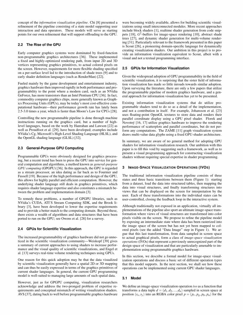
Fig. 3. Image-space mapping using an IVO (image-space visualizationoperator) shader. Each data tuple dx,y ∈ D is mapped to its correspond-ing RGBA pixel px, ∈ P for screen position (x,y). D is a data buffer ras-terized at the same resolution (n×m) as the RGBA framebuffer P. Notethat for overlapping visualizations, like 2D scatterplots, there may actu-ally be several data tuples defined for each screen position.)

Fragment shaders are installed globally in the graphics API for a set ofprimitives. Because visual structures typically have different classes ofgraphical entities—for example, a node-link diagram consists of edgeentities and node entities—we introduce the concept of layers, whichare a set of graphical entities and a corresponding IVO for transform-ing them to color pixels. Some layers in a visual structure may serve apurely aesthetic purpose or may not carry image-space data, in whichcase the IVO will be the identity function.

Figure 4 shows our implementation model for mapping IVOs to theGLSL [32] shader language. Like all fragment shaders, and in keepingwith the IVO model, the output is always a colored RGBA pixel. In ourprototype implementation, the input data tuple d is passed simply asthe color of the primitive. In other words, when drawing the graphicalentities for a layer, the program will simply pass image-space data bysetting the data as the color for each primitive (such as the marks ina scatterplot). A more scalable solution that would support a largenumber of data points di in d would be to transfer the data as floating-point textures using the multitexture functionality of modern graphicscards. Essentially, instead of reading from a single input color, theshader would sample each texture buffer to retrieve the n data values.

Fig. 4. The GPUVis IVO shader model. Generated GLSL fragmentshaders accept data values on a per-fragment level encoded in theOpenGL color and texture coordinate variables, as well as meta-values(e.g. filters, colors, scaling) as uniform arguments on a per-layer level.

Beyond the data inputs in the color argument, the shader IVO will re-ceive the local coordinates of a fragment in a primitive using its texturecoordinates. To draw a glyph, the application would simply draw a 2Drectangle (or another graphics primitive) and initialize the texture co-ordinates from (0,0) to (1,1) for the respective corner points. Thesevalues will define the local coordinate system for the primitive.

To illustrate our GLSL shader model, we return to the example IVO inFigure 2. Figure 5 shows GLSL code that implements this particularIVO. Each participating component (IVC) in the IVO has been denotedin the source with a comment and a number (e.g., (1)). Figure 6shows a screenshot of a 2D scatterplot drawn using this IVO.

4.3 Implementing Data Image Feedback

To implement the data image feedback of Section 3.4, we introduce aG-buffer [33] as an intermediate rendering target implemented usingan off-screen framebuffer object (FBO). The OpenGL FBO extensionenables us to use the graphics hardware to render the data primitives

uniform vec4 scale, minF, maxF;void main() {

vec4 d = gl_Color;float lx = gl_TexCoord[0].s;float ly = gl_TexCoord[0].t;// Computation (1)d /= scale;// Filtering (2)if (d[0] < minF[0] || d[0] > maxF[0]|| d[1] < minF[1] || d[1] > maxF[1]|| d[2] < minF[2] || d[2] > maxF[2]|| d[3] < minF[3] || d[3] > maxF[3])

discard;// Barchart glyph (3)float v = -1.0;if (lx < 0.25 && ly < data[0])

v = data[0];else if (lx < 0.5 && ly < data[1])

v = data[1];else if (lx < 0.75 && ly < data[2])

v = data[2];else if (ly < data[3])

v = data[3];// Color mapping (4)if (v == -1.0)

gl_FragColor = vec4(1, 1, 1, 1);else

gl_FragColor = vec4(v, 0, 0, 1);}

Fig. 5. GLSL fragment shader for an example IVO.

Fig. 6. Scatterplot visualization for a car dataset (9 dimensions, 406cases) with a barchart glyph IVO.

to a floating-point off-screen render target (one per layer). We canthen read back this buffer, analyze it, and use the results to producethe final color framebuffer image. Note that there is no need to redrawthe data image until the view changes—instead, we transform the dataimage into a framebuffer by drawing a single 2D rectangle coveringthe whole screen and with the data image as a texture.

Figure 7 gives an example of a dynamic colorscale adaption techniqueimplemented using data image feedback and a shader IVO. A similarapproach could be used for a query-by-example [15] implementation.

5 DOMAIN-SPECIFIC VISUAL PROGRAMMING ENVIRONMENT

So far in this paper, we have proposed a theoretical extension to the in-formation visualization pipeline and introduced a new class of image-space visualization operations. We have also shown how these op-erations can be easily mapped to current shader languages, and givenexamples for the GLSL shader language. However, there are two mainobstacles remaining for making this approach generally usable:

Fig. 7. Dynamic colorscale optimization IVO. We draw the data to a G-buffer FBO, read it back, analyze the contents of the sampling lens, andthen change the colorscale optimized for the lens contents.

Expertise. Writing shaders requires a great level of programming ex-pertise, increasing the gap between expert developers and visu-alization professionals [31]; and

Conceptual mismatch. There is a conceptual mismatch between thegraphics-centric shader language, and the data-centric visualiza-tion operations [3, 26].

In other words, there is a need for a domain-specific language, built ontop of the actual shader language, that maps directly to the visualiza-tion domain and that does not require shader expertise to use.

5.1 System Architecture

We have developed GPUVIS, a visualization environment supportingimage-space visualization operations. To fulfill the above need, weprovide a visual programming interface for building IVOs.

Fig. 8. GPUVis system architecture. Visualizations are loaded as plu-gins depending on the type of dataset and consists of one or severallayers, each with its own IVO. Depending on the parameters exposedby the IVO, the application control panel will be populated with the cor-responding GUI controls to specify the parameters.

Figure 8 shows the modular GPUVis system architecture. The systemis based around a central dataset structure. Depending on the type ofthe data the user loads into the dataset, the environment will instantiatea corresponding visualization plugin (i.e., a scatterplot for multidimen-sional data, a treemap [34] for hierarchical data, a node-link diagramfor graphs, etc). Each visualization manages one or more layers (asdefined above), and each layer contains the graphical primitives mak-ing up the visualization and an IVO—editable by the user in a visualIVO editor (described in detail in Section 5.3).

5.2 User Interaction

Interaction is managed by the GPUVis control panel, a tabbed layoutwith one tab page per each layer. The user can control the data map-

ping between the dataset and the graphical primitives for each layerusing controls in the panel. General interaction techniques, such aszoom, pan, and drill-down, are implemented by each visualization.

IVOs in our visualization environment are built using the visual IVOeditor. Beyond the actual operation (implemented as a GLSL shader),an IVO also contains a symbol table of parameters and their types(such as color, value, interval, etc). Every time a particular layer’sIVO is edited, the system will iterate over the symbol table and createa matching user interface component for controlling the parameter (forexample, a color generates a color chooser dialog, a bounded valuegenerates a slider, and an interval generates a range slider [40]).

5.3 Visual IVO Editor

In order to circumvent the need for expert programming skills whenconstructing custom shader IVOs, the GPUVis system contains a vi-sual IVO editor. This visual programming environment abstracts IVOdevelopment into a dataflow-style pipeline composed of componentblocks, each representing an image-space visualization component(ISVC, see Section 3.3), implemented using a small segment of GLSLshader code. The blocks are arranged and connected to represent thedesired image-space visual operation, and a GLSL shader is generatedfrom the graphically described pipeline. This generated shader canthen be directly used in the visualization environment.

5.3.1 Background

Visual programming [5, 30] is the use of graphics to specify a program.One of the many uses of visual programming languages (VPLs) is forgraphics and visualization. ConMan [21] is a VPL for building graph-ical applications by connecting components in an approach similar toUNIX pipes. Building on the same design principles is AVS [37], avisual programming system for scientific visualization where each in-dividual module may have an associated user interface component. Inrelated work, Burnett et al. [4] discuss the use of VPLs for interactivelysteering and modifying scientific computations through visualization.

More recent visualization systems have also been designed around avisual programming paradigm and serve as inspiration for our work.GeoVISTA Studio [25] is a flow-based visual programming environ-ment built using JavaBeans components for geographic visualization.The DataMeadow [12] visual exploration system combines a dataflowVPL with multidimensional visualization techniques and annotationfunctionality. Finally, Improvise [38] is a highly configurable andadaptive visualization system for multiple coordinated views.

5.3.2 Visual Pipeline Construction

Custom IVO creation begins with the visual depiction of the desiredoperation. As stated above, this is accomplished through the use ofobjects called component (ISVC) blocks. These blocks represent afew lines of GLSL shader code that perform a distinct function. Eachblock has inputs and outputs, allowing it to accept data from precedingblocks, manipulate that data according to its particular function, andmake the result available for succeeding blocks. Figure 9 shows theanatomy of two different types of blocks.

Fig. 9. Sample component blocks. The block on the left computes theaverage of the 2 input values, while the block on the right allows thepipeline designer to provide the IVO with a constant value.

The specific properties of a given ISVC block (such as number of in-puts/outputs and the corresponding GLSL shader code) are organized

in individual XML files. These files are loaded when the editor starts,and are made available to the designer in the pipeline toolbox. Thedesired blocks can then be dragged from the toolbox and dropped inthe pipeline workbench. Once there, the blocks can be arranged andconnected to form the envisioned pipeline. Figure 10 shows the visualprogramming environment as well as a sample pipeline.

Fig. 10. Visual programming environment and sample shader pipeline.This pipeline corresponds to a shader very similar to the one describedin Figure 2, excluding the filtering step. Data flows through the pipelinefrom left to right. i0, i1, i2, i3 are the four input data values for the bargraph and R, G, B, A are the four color components of the output pixel.

Since the assembled visual pipeline corresponds to actual GLSLshader code, a certain level of awareness of the underlying IVO modelis needed. For example, since an IVO always produces a pixel colorvalue, every pipeline must end with the four elements of that colorvalue (as in Figure 10). Also, the values that each block accepts asinputs, and the values that it makes available as outputs, have datatypes (float, vec3, vec4, etc). Connected outputs and inputs must havematching data types for the IVO to be valid.

5.3.3 Code Generation

Once the designer is satisfied with the visual representation of the IVOpipeline, actual GLSL code must be generated from the diagram. Thisis done in two separate stages using a breadth-first traversal:

1. Dependency Resolution. If a given block depends on anotherblock’s output, the output variable of the first block must be as-signed correctly to the input variable of the second block. De-pendencies must be propagated through the whole pipeline.

2. Code Fragment Assembly. Once all dependencies have beenresolved, the individual code fragments must be assembled to-gether in the order specified by the pipeline design.

For a given visualization to have meaningful user interaction, addi-tional information is needed. When the shader code is generated, asymbol table is also built for all uniform variables that the shader de-pends on. These uniform variables are constant on a per-layer basis,and can be set by the user through the use of variable appropriate com-ponents (sliders, range-sliders, color choosers, and spinners).

5.4 Examples

The GPUVis environment currently supports multidimensional scat-terplot visualizations as well as basic node-link and treemap [34] vi-

sualizations. We also provide a separate colorscale optimization tool(depicted in Figure 7) built using the principles discussed in this paper.

Scatterplot: As mentioned earlier, Figure 6 shows the scatterplotvisualization in the GPUVis system, here depicted with a glyph-basedshader for a car dataset. Each glyph is drawn by the CPU and rep-resents a car in the scatterplot. The GPU fills in the contents of theglyph to shows additional dimensions beyond the two captured by theorthogonal axes of the plot. By changing the data flow mappings, thedata displayed in the barcharts can be changed. Range sliders gener-ated for the IVO allows for filtering out data based on each car’s data.

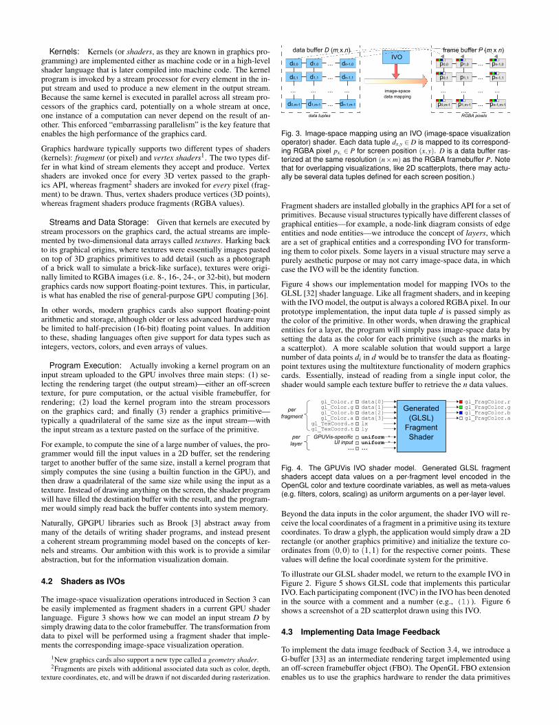
Node-Link Diagram: Figure 11 shows the GPUVis node-link di-agram being used for visualizing a file system hierarchy. The visual-ization is split into two layers, one for nodes and one for edges. Nodesand their layout are handled by the CPU, but their individual glyphsare drawn by the GPU. In the example, the user has added a glyph IVOto the node layer for drawing a polar barchart on the surface of eachnode. This glyph can be utilized to display attributes associated with afile, such as file size, time since last modified, and time since creation.

Fig. 11. Node-link visualization with a polar barchart glyph IVO.

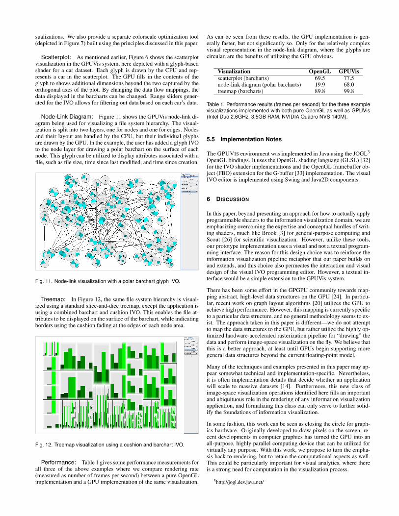
Treemap: In Figure 12, the same file system hierarchy is visual-ized using a standard slice-and-dice treemap, except the application isusing a combined barchart and cushion IVO. This enables the file at-tributes to be displayed on the surface of the barchart, while indicatingborders using the cushion fading at the edges of each node area.

Fig. 12. Treemap visualization using a cushion and barchart IVO.

Performance: Table 1 gives some performance measurements forall three of the above examples where we compare rendering rate(measured as number of frames per second) between a pure OpenGLimplementation and a GPU implementation of the same visualization.

As can be seen from these results, the GPU implementation is gen-erally faster, but not significantly so. Only for the relatively complexvisual representation in the node-link diagram, where the glyphs arecircular, are the benefits of utilizing the GPU obvious.

Visualization OpenGL GPUVisscatterplot (barcharts) 69.5 77.5node-link diagram (polar barcharts) 19.9 68.0treemap (barcharts) 89.8 99.8

Table 1. Performance results (frames per second) for the three examplevisualizations implemented with both pure OpenGL as well as GPUVis(Intel Duo 2.6GHz, 3.5GB RAM, NVIDIA Quadro NVS 140M).

5.5 Implementation Notes

The GPUVIS environment was implemented in Java using the JOGL3

OpenGL bindings. It uses the OpenGL shading language (GLSL) [32]for the IVO shader implementations and the OpenGL framebuffer ob-ject (FBO) extension for the G-buffer [33] implementation. The visualIVO editor is implemented using Swing and Java2D components.

6 DISCUSSION

In this paper, beyond presenting an approach for how to actually applyprogrammable shaders to the information visualization domain, we areemphasizing overcoming the expertise and conceptual hurdles of writ-ing shaders, much like Brook [3] for general-purpose computing andScout [26] for scientific visualization. However, unlike these tools,our prototype implementation uses a visual and not a textual program-ming interface. The reason for this design choice was to reinforce theinformation visualization pipeline metaphor that our paper builds onand extends, and this choice also permeates the interaction and visualdesign of the visual IVO programming editor. However, a textual in-terface would be a simple extension to the GPUVis system.

There has been some effort in the GPGPU community towards map-ping abstract, high-level data structures on the GPU [24]. In particu-lar, recent work on graph layout algorithms [20] utilizes the GPU toachieve high performance. However, this mapping is currently specificto a particular data structure, and no general methodology seems to ex-ist. The approach taken in this paper is different—we do not attemptto map the data structures to the GPU, but rather utilize the highly op-timized hardware-accelerated rasterization pipeline for “drawing” thedata and perform image-space visualization on the fly. We believe thatthis is a better approach, at least until GPUs begin supporting moregeneral data structures beyond the current floating-point model.

Many of the techniques and examples presented in this paper may ap-pear somewhat technical and implementation-specific. Nevertheless,it is often implementation details that decide whether an applicationwill scale to massive datasets [14]. Furthermore, this new class ofimage-space visualization operations identified here fills an importantand ubiquituous role in the rendering of any information visualizationapplication, and formalizing this class can only serve to further solid-ify the foundations of information visualization.

In some fashion, this work can be seen as closing the circle for graph-ics hardware. Originally developed to draw pixels on the screen, re-cent developments in computer graphics has turned the GPU into anall-purpose, highly parallel computing device that can be utilized forvirtually any purpose. With this work, we propose to turn the empha-sis back to rendering, but to retain the computational aspects as well.This could be particularly important for visual analytics, where thereis a strong need for computation in the visualization process.

3http://jogl.dev.java.net/

7 CONCLUSIONS AND FUTURE WORK

In this paper, we have explored ways to harness programmable GPUsfor information visualization. The major hurdle against adopting thesemethods for information visualization has been the mismatch betweenabstract data structures such as trees, graphs, and free text and thefloating-point model of the graphics hardware. We consider this workto present two major contributions towards such adoption: (1) the the-oretical concept of image-space visualization operations (IVOs) thatsuggest how to utilize shaders for information visualization in the firstplace, and (2) the practical implementation of a visual programmingenvironment for building shaders that implement the IVO concept.

However, this is only an initial step towards utilizing the full potentialof graphics hardware. The approach we take here is limited to image-space operations in the ultimate transformation from data to coloredpixels in the visualization pipeline, and does not support offloadingwhole visualizations or complex datasets to the GPU. In the future,we would like to integrate even more computational components inthe visualization pipeline, especially for supporting visual analyticsapplications. Also, we would like to explore the use of CUDA orOpenCL instead of GLSL as an output language.

ACKNOWLEDGEMENTS

Thanks to members of the AVIZ and INSITU research groups for theirfeedback on the early stages of this research. This work was conductedunder the Purdue SURF 2009 program for undergraduate research.

REFERENCES

[1] G. D. Abram and T. Whitted. Building block shaders. In ComputerGraphics (SIGGRAPH ’90 Proceedings), volume 24, pages 283–288,Aug. 1990.

[2] J. Bertin. Semiology of graphics. University of Wisconsin Press, 1983.[3] I. Buck, T. Foley, D. Horn, J. Sugerman, K. Fatahalian, M. Houston, and

P. Hanrahan. Brook for GPUs: Stream computing on graphics hardware.ACM Transactions on Graphics, 23(3):777–786, Aug. 2004.

[4] M. Burnett, R. Hossli, T. Pulliam, B. V. Voorst, and X. Yang. Towardvisual programming for steering scientific computations. IEEE Compu-tational Science & Engineering, 1(4):44–62, 1994.

[5] M. Burnett and D. McIntyre. Special issue on visual programming. IEEEComputer, 28(3), 1995.

[6] S. K. Card and J. Mackinlay. The structure of the information visualiza-tion design space. In Proceedings of the IEEE Symposium on InformationVisualization, pages 92–99, 1997.

[7] S. K. Card, J. D. Mackinlay, and B. Shneiderman, editors. Readingsin information visualization: Using vision to think. Morgan KaufmannPublishers, San Francisco, 1999.

[8] E. H. Chi and J. T. Riedl. An operator interaction framework for visual-ization systems. In Proceedings of the IEEE Symposium on InformationVisualization, pages 63–78, 1998.

[9] R. L. Cook. Shade trees. In Computer Graphics (Proceedings of SIG-GRAPH 1984), pages 223–231, 1984.

[10] M. Eissele, D. Weiskopf, and T. Ertl. The G2-buffer framework. In Sim-ulation und Visualisierung 2004 (SimVis 2004), pages 287–298, 2004.

[11] N. Elmqvist, T.-N. Do, H. Goodell, N. Henry, and J.-D. Fekete. ZAME:Interactive large-scale graph visualization. In Proceedings of the IEEEPacific Visualization Symposium, pages 215–222, 2008.

[12] N. Elmqvist, J. Stasko, and P. Tsigas. DataMeadow: A visual canvasfor analysis of large-scale multivariate data. Information Visualization,7:18–33, 2008.

[13] K. Engel, M. Hadwiger, C. Rezk-Salama, and D. Weiskopf. Real-timeVolume Graphics. AK Peters, 2006.

[14] J.-D. Fekete and C. Plaisant. Interactive information visualization of amillion items. In Proceedings of the IEEE Symposium on InformationVisualization, pages 117–124, 2002.

[15] K. Fishkin and M. C. Stone. Enhanced dynamic queries via movablefilters. In Proceedings of the ACM CHI’95 Conference on Human Factorsin Computing Systems, pages 415–420, 1995.

[16] M. Florek. Using modern hardware for interactive information visualiza-tion of large data. Master’s thesis, Faculty of Mathematics, Physics andInformatics, Comenius University, Bratislava, 2006.

[17] M. Florek and M. Novotny. Interactive information visualization usinggraphics hardware. In Poster Proceedings of Spring Conference on Com-puter Graphics, 2006.

[18] N. Folkegard and D. Wesslen. Dynamic code generation for realtimeshaders. In Proceedings of SIGGRAD, pages 11–15, 2004.

[19] A. Fournier and D. Fussell. On the power of the frame buffer. ACMTransactions on Graphics, 7(2):103–128, 1988.

[20] Y. Frishman and A. Tal. Multi-level graph layout on the GPU. IEEETransactions on Visualization and Computer Graphics, 13(6):1310–1319, 2007.

[21] P. E. Haeberli. ConMan: A visual programming language for interac-tive graphics. In Computer Graphics (SIGGRAPH ’88 Proceedings), vol-ume 22, pages 103–111, Aug. 1988.

[22] P. Hanrahan and J. Lawson. A language for shading and lighting calcula-tions. In Computer Graphics (SIGGRAPH ’90 Proceedings), volume 24,pages 289–298, Aug. 1990.

[23] J. Johansson, P. Ljung, M. Jern, and M. Cooper. Revealing structurein visualizations of dense 2D and 3D parallel coordinates. InformationVisualization, 5(2):125–136, 2006.

[24] A. E. Lefohn, S. Sengupta, J. Kniss, R. Strzodka, and J. D. Owens. Glift:Generic, efficient, random-access GPU data structures. ACM Transac-tions on Graphics, 25(1):60–99, Jan. 2006.

[25] M. G. M. Takatsuka. GeoVISTA Studio: A codeless visual programmingenvironment for geoscientific data analysis and visualization. Journal ofComputers & Geosciences, 2002.

[26] P. S. McCormick, J. T. Inman, J. P. Ahrens, C. D. Hansen, and G. Roth.Scout: A hardware-accelerated system for quantitatively driven visual-ization and analysis. In Proceedings of the IEEE Conference on Visual-ization, pages 171–178, 2004.

[27] M. McGuire, G. Stathis, H. Pfister, and S. Krishnamurthi. Abstract shadetrees. In Proceedings of the ACM Symposium on Interactive 3D Graphicsand Games, pages 79–86, 2006.

[28] J. D. Owens, D. Luebke, N. Govindaraju, M. Harris, J. Kruger, A. E.Lefohn, and T. J. Purcell. A survey of general-purpose computation ongraphics hardware. Computer Graphics Forum, 26(1):80–113, March2007.

[29] K. Proudfoot, W. Mark, S. Tzvetkov, and P. Hanrahan. A real time proce-dural shading system for programmable graphics hardware. In Proceed-ings of SIGGRAPH 2001, pages 159–170, 2001.

[30] T. I. Robert B. Grafton. Special issue on visual programming. IEEEComputer, 18(8), 1985.

[31] F. Roßler, R. P. Botchen, and T. Ertl. Dynamic shader generation forGPU-based multi-volume ray casting. IEEE Computer Graphics and Ap-plications, 28(5):66–77, Sept./Oct. 2008.

[32] R. J. Rost, J. M. Kessenich, and B. Lichtenbelt. The OpenGL ShadingLanguage. Addison-Wesley, 2004.

[33] T. Saito and T. Takahashi. Comprehensible rendering of 3-D shapes.Computer Graphics (SIGGRAPH’90), 24(4):197–206, 1990.

[34] B. Shneiderman. Tree visualization with tree-maps: A 2-D space-fillingapproach. ACM Transactions on Graphics, 11(1):92–99, Jan. 1992.

[35] B. Shneiderman. The eyes have it: A task by data type taxonomy forinformation visualizations. In Proceedings of the IEEE Symposium onVisual Languages, pages 336–343, 1996.

[36] C. J. Thompson, S. Hahn, and M. Oskin. Using modern graphics archi-tectures for general-purpose computing: A framework and analysis. InProceedings of IEEE/ACM International Symposium on Microarchitec-ture, pages 306–317, 2002.

[37] C. Upson, T. Faulhaber, D. Kamins, D. Laidlaw, D. Schlegel, J. Vroom,R. Gurwitz, and A. van Dam. The application visualization system: Acomputational environment for scientific visualization. IEEE ComputerGraphics and Applications, 9(4):30–42, July 1989.

[38] C. Weaver. Building highly-coordinated visualizations in Improvise. InProceedings of the IEEE Symposium on Information Visualization, pages159–166, 2004.

[39] D. Weiskopf. GPU-Based Interactive Visualization Techniques. SpringerVerlag, 2006.

[40] C. Williamson and B. Shneiderman. The dynamic HomeFinder: Eval-uating dynamic queries in a real-estate information exploration system.In Proceedings of the ACM SIGIR Conference on Research and Develop-ment in Information Retrieval, pages 338–346, 1992.