toxic workers - harvard university

Toxic Workers

CitationHousman, Michael, and Dylan Minor. "Toxic Workers." Harvard Business School Working Paper, No. 16-057, October 2015.

Permanent linkhttp://nrs.harvard.edu/urn-3:HUL.InstRepos:23481825

Terms of UseThis article was downloaded from Harvard University’s DASH repository, and is made available under the terms and conditions applicable to Other Posted Material, as set forth at http://nrs.harvard.edu/urn-3:HUL.InstRepos:dash.current.terms-of-use#LAA

Share Your StoryThe Harvard community has made this article openly available.Please share how this access benefits you. Submit a story .

Accessibility

http://nrs.harvard.edu/urn-3:HUL.InstRepos:23481825

http://nrs.harvard.edu/urn-3:HUL.InstRepos:dash.current.terms-of-use#LAA

http://nrs.harvard.edu/urn-3:HUL.InstRepos:dash.current.terms-of-use#LAA

http://osc.hul.harvard.edu/dash/open-access-feedback?handle=&title=Toxic%20Workers&community=1/3345929&collection=1/3345930&owningCollection1/3345930&harvardAuthors=9b94b84e41a41e5f2eb051bc94bf69a9&department

https://dash.harvard.edu/pages/accessibility

Toxic Workers

Michael Housman Dylan Minor

Working Paper 16-057

Working Paper 16-057

Copyright © 2015 by Michael Housman and Dylan Minor

Working papers are in draft form. This working paper is distributed for purposes of comment and discussion only. It may not be reproduced without permission of the copyright holder. Copies of working papers are available from the author.

Toxic Workers Michael Housman Cornerstone OnDemand

Dylan Minor Harvard Business School

Toxic Workers∗

Michael Housman

Cornerstone OnDemand

Dylan Minor

Kellogg School of Management, Northwestern University

October, 2015

Abstract

While there has been a lot of research on finding and developing top per-

formers in the workplace, less attention has been paid to the question of how

to manage those workers who are harmful to organizational performance. In

extreme cases, in addition to hurting performance, such workers can gener-

ate enormous regulatory and legal liabilities for the firm. We explore a large

novel dataset of over 50,000 workers across 11 different firms to document a

variety of aspects of workers’characteristics and circumstances that lead them

to engage in "toxic" behavior. We also find that avoiding a toxic worker (or

converting him to an average worker) enhances performance to a much greater

extent than replacing an average worker with a superstar worker.

Keywords: human resource management, misconduct, worker productivity,

ethics, superstar

∗The authors thank Steve Morseman for his invaluable research support. Comments from Jen-nifer Brown and Lamar Pierce are gratefully acknowledged. Also thanked are the participants fromthe Academy of Management meeting (2015), Alliance for Research on Corporate Sustainabilityconference (2015), Goethe University, Harvard Business School I&I (2014), NBER Summer Insti-tute (2015), Northwestern Law School, Queens University, and University of Cologne. This researchwas conducted in collaboration with the Workforce Science Project of the Searle Center for Law,Regulation and Economic Growth at Northwestern University.

1

1 Introduction

There is an abundance of work that explores how to find, develop, and incentivize

top performers so as to enhance organizational performance (Lazear and Oyer (2007)

and Gibbons and Roberts (2013)). What this work makes clear is that hiring the

right people is very important. Finding the positive outliers– the "stars"– can sub-

stantially increase performance (e.g., Azoulay et al. (2010), Sauermann and Cohen

(2010), and Oettl (2012)). However, there are outliers from the other side of the

distribution that are much less studied: those workers who are harmful to an or-

ganization’s performance (Banerjee et al. (2012) and Pierce and Balasubramanian

(2015)). At their most harmless, these workers could simply be a bad fit, leading to

premature termination and a costly search for and training of a new worker. How-

ever, more damaging to the firm is a worker who engages in behavior that adversely

affects fellow workers or other company assets; we label this type of worker "toxic."

A toxic worker may engage in sexual harassment, workplace violence, fraud,or some

other breach of important company policy or governmental law. In its most dramatic

form, such worker misconduct can cost a firm billions of dollars, as evidenced by JP

Morgan’s "London Whale" incident with Bruno Iksil.1 At another extreme, such

workers can even mortally harm current or past colleagues, as tragically witnessed in

the fatal shooting of WDBJ-TV reporters by their former colleague.2 But even rela-

tively modest levels of toxic behavior can cause major organizational cost, including

customer loss, loss of employee morale, increased turnover, and loss of legitimacy

among important external stakeholders (Robinson and Bennett (1995), Litzky et al.

(2006), Ermongkonchai (2010) and MacLean et al. (2010)).

The causes of worker misconduct are varied. There is consistent evidence that

incentives can play a very important role in causing adverse outcomes (e.g., see

Oberholzer-Gee and Wulf (2012), Larkin (2014), and Minor (2014)). There is also

1See http://www.bloombergview.com/quicktake/the-london-whale. In this case, it was ulti-mately not Mr. Iksil himself who was charged (he cooperated with authorities), but rather hissupervisor and junior trader.

2http://www.cbsnews.com/news/virginia-wdbj-station-shooting-alleged-gunman-posted-video-of-shooting-on-social-media/

2

evidence suggesting that a worker’s personal characteristics are important in deter-

mining his ethical behavior (e.g., see Ford and Richardson (1994) and Loe et al.

(2000)). Lazear and Oyer (2007) suggest that the selection of workers plays a role

at least as important, if not more important than incentives in generating outcomes.

Thus, one approach to managing toxic workers– and the approach we focus on in

this paper– is simply avoiding them. However, in order to do so, we must be able to

identify them ahead of time. By exploring the actual conduct and characteristics of

many workers that are quasi-randomly placed across and within different organiza-

tions, we identify several individual predictors of toxic workers: overconfidence, poor

service-orientation, and a vision of themselves as rule followers.

In addition to these predictors, we also find evidence that an employee’s work en-

vironment contributes to the likelihood of him becoming a toxic worker (e.g., Vardi

(2001) , Greve et al. (2010), and Pierce and Snyder (2014)). Our paper complements

the work of Pierce and Snyder (2014) who show that in the setting of automobile

emissions testing a worker’s environment has significant effects on her individual

ethical conduct. Moreover, alongside showing that this environmental effect is also

present in a broader setting, we are able to compare the importance of an individual’s

characteristics and identify which individual characteristics matter in determining

outcomes, which adds substantially to our explanatory power. Pierce and Snyder’s

(2014) findings about the impact of workplace environment, while important, ex-

plained only the minority of the variation of outcomes.

We also document other features of toxic workers. Specifically, we find that toxic

workers produce greater output than the average worker. Thus, as in Gino and Ariely

(2012) and Frank and Obloj (2014), we find that there is a potential trade-off when

employing an unethical person: they are corrupt, but they excel in work performance.

This might explain how a toxic worker can persist in an organization. However, we

find that when their productivity is examined more closely, their quality of work is

subpar. Thus, they produce at a faster rate, but at lower quality than their average

non-toxic peers.

Finally, we estimate the value of finding a "superstar," defined as workers in the

top 1% of productivity, versus the value of avoiding a toxic worker. Succeeding in

3

the latter generates returns of nearly two-to-one compared to those generated when

firms hire a superstar. This suggests more broadly that "bad" workers may have a

stronger effect on the firm than "good" workers. In many other fields and disciplines

researchers have found that a negative has a stronger impact than a positive. For

example, in the domain of finance, loss aversion recognizes that in terms of magnitude

losses have more of an impact than gains (see Tversky & Kahneman (1992)). In the

discipline of psychology it is a generally accepted principle that bad experiences have

a stronger hold on our psyches than good ones (Baumeister et al. (2001)). Finally, in

the field of linguistics, it has been found that humans preferentially attend to negative

words over positive or neutral ones (Estes and Adelman (2008)). It is no surprise to

us that these findings hold true in the field of human resource management, as well.

Much of the past research on unethical worker conduct has been based on surveys,

self-reports, and intention-based outcomes (Weaver and Trevino (1999) and Green-

berg (2002)). Bertrand and Mullainathan (2001) suggest that the mixed results of

this past work likely stem from the challenge of empirically examining subjective

data. For our setting, we define toxic workers as those who are actually terminated

for toxic behavior. Thus, this paper complements this important work by linking

personal characteristics of workers quasi-randomly placed within organizations with

objective conduct outcomes across a very large, novel data set.

An alternative to avoiding toxic workers altogether, is to reform those already

in the organization. With resource constraints it may not be feasible for some, if

not most, organizations to pursue this second path. However, since we find that a

worker’s environment is also important in influencing toxic outcomes, there is some

hope that through judicious management of a worker’s environment, toxicity can

be reduced. Nonetheless, further exploring this channel is beyond the scope of the

current paper.

The balance of the paper is organized as follows. The next section develops a

theoretical understanding of the problem of toxic workers and explores how we can

identify their origins. Section Three presents our main empirical results. Section

Four provides a discussion, and our final section concludes.

4

2 Theoretical Considerations: The Person and the

Situation

In this section, we consider a simple theoretical setting to illustrate the link between

theory and our identification strategy. We begin by assuming a simple world in which

all workers are the same and all environments are the same. That is, the person and

the situation are always the same. This will serve as a baseline that will then be

modified by allowing for different individuals and different situations one at a time.

In this setting, all workers can engage in toxic behavior in a given period. Once they

engage in such behavior, they are dubbed a toxic worker.3

First assume that P represents the probability that a person will engage in some

toxic behavior4 in a given period. In a worker’s first period, she has a P chance of

engaging in toxic behavior. This means that she has a 1 − P chance of working in

the next period, assuming a toxic worker is removed from the worker pool. Hence,

the chance that a worker makes it beyond period t is (1− P )t , 5 which we denoteas the survival rate S (t) . In contrast, the chance that a worker does not make it to

period t is 1 − (1− P )t , which we denote as the failure rate F (t) . Recall that thehazard rate, where f (t) is the density of F (t) , is then defined as

3In the general case, with different individuals and situations, it makes more sense to define toxicworkers as those who are more likely to engage in toxic behavior than those who or not. However,here all workers are toxic workers in that sense, so we use the term toxic worker to denote whensuch a worker actively engages in toxic behavior.

4Here, and throughout when we use the term toxic behavior, we are assuming the kind ofbehavior that is observable (or that its effects are observable).

5Note that with this setup it is equivalent to assume that workers have a constant propensityto engage in misconduct and finally do so in a given period with probability P, after which theyare removed from the worker pool, and to assume that workers always engage in a constant levelof misconduct and are finally caught and removed with probability P. For this study, what we willactually observe is the removal of a worker (i.e., a termination) who has engaged in toxic behavior.

5

h (t) :=f (t)

S (t)

=− ln (1− P )t (1− P )t

(1− P )t

= − ln (1− P )t .

The hazard rate tells us the chance that a worker will be a toxic worker at

time t, given that she has not yet been toxic up until time t. Not only is this an

intuitive measure to consider, but there is a long, rich history of estimating hazard

rates. In this simple setup of a constant chance of engaging in toxic behavior for

all periods, for all people and all situations, the hazard rate would then simple be a

linearly increasing function of time, since − ln (1− P )t = −t ln (1− P ) . Of course,in practice, we do not expect this to be true. In fact, we expect that the hazard

rate is likely a very complex function. For example, even if all people and situations

were the same, it could take more than one period for a worker to engage in toxic

behavior; perhaps it takes more than one period to learn about and take advantage

of an opportunity. In this case, P would increase over time. Alternatively, perhaps

a person is more likely to engage in toxic behavior during the formative days and

months at a new position; as time passes, she becomes better integrated and less

likely to be toxic. Many other possibilities abound. Thus, it seems important not to

assume some ex-ante relationship between time and the hazard rate. In our setting,

we will refrain from making this assumption for our baseline hazard rate by instead

specifying an overall hazard rate of engaging in toxicity for a particular person over

time as

h (t) f (t|X) ,

where h (t) is allowed to have an arbitrary relationship between the hazard rate

and time and can be viewed as the average relationship between time and the hazard

rate. In contrast, the function f (t|X) takes on a value greater or less than 1 as a

6

function of (potentially) both the person and situation across time. In this sense,

this approach follows the spirit of Trevino (1986) to simultaneously consider both

the person and the situation. Specifically, f (t|X) is a function of the person andthe situation at time t, which are captured by the matrix X. In its simplest form,

we could assume a world with workers that are sometimes toxic at a periodic rate

of h (t) and another set of workers who are never toxic. Thus, f (t|X) would simplybe an indicator function, taking on the value of 1 or 0, depending on whether the

worker is toxic.

For a richer example, assume after 365 days that an average remaining worker

has a 5% chance of engaging in toxic behavior on day 366; this means h (366) = .05.

However, this chance could increase or decrease as a function of the honesty of a

particular worker, as well as her job position. The function f (t|X) is then greateror less than 1 depending on the person (e.g., her level of honesty) and the situation

(e.g., her particular job position) at a particular point in time. This flexible setup

allows us to model a myriad of real-world settings and is the approach we will use

in our estimation, as outlined below. However, first we consider some settings of

the person and the situation that we can both measure in our study and expect to

matter in terms of outcome.

2.1 Factors of the Person and the Situation

In principle, there are some identifiable factors that are likely to predict toxic behav-

ior, especially when studying actual outcomes. Here we discuss those that we can

measure in our data. The empirical proxies for these factors are discussed in section

3.1.

It is well established that other-regarding preferences determine the kinds of

actions people choose and that people have heterogenous levels of other-regardingness

(e.g., see Andreoni and Miller (2002) and Fisman, Kariv and Markovitz (2007)).

All things equal, those that are less other-regarding should be more predisposed to

toxicity, as they do not fully internalize the cost that their behavior imposes on others.

A way to capture one’s degree of other-regardingness is to identify how concerned

7

one is about taking care of another’s needs. Those that are service-oriented exhibit

care for the needs of others. In contrast, those that show little concern for another’s

interests are less likely to refrain from damaging others and their property. Thus,

ceterus paribus, those with poor service-orientation should be more likely to engage

toxic behavior.

Hypothesis 1: Workers with poor service orientation are more likely tobe toxicOutside of the business ethics literature, there are also some consistent findings

that overconfidence contributes to adverse behavior and outcomes. Petit and Bol-

laert (2011) document a set of important management and finance papers that have

established this link. Broadly, there at least two dimensions that might manifest

overconfidence. Thus, toxic behavior should be increasing alongside a worker’s de-

gree of confidence, holding all else constant.

Hypothesis 2: Overconfident workers are more likely to be toxicAn apparently straightforward factor for measuring the propensity of misconduct

is whether or not a worker agrees that rules should always be followed. It would seem

that those who always follow rules are likely to follow ethical rules, as well. However,

in certain situations, a rule might need to be broken, perhaps to do the "right thing."

History is replete with such examples, and it has become a self-evident truth that

some rules are meant to be broken. Thus, subjects who admit that sometimes rules

should be broken are likely more honest than those who maintain that rules should

always be followed. It also seems self-evident that those who are honest are less likely

to engage in misconduct, all things equal. Taken together, this suggests that those

claiming rules should always be followed are actually more likely to break the rules

via toxic conduct.

Hypothesis 3: Workers that claim the rules should never be broken aremore likely to be toxicPossibly the most important factor in determining whether the work environment

will increase the likelihood of misconduct is the likelihood of the worker’s colleagues

to engage in toxic behavior. Pierce and Snyder (2008) find strong evidence that there

are ethical-worker peer effects, akin to productivity peer effects. Thus, using Pierce

8

and Snyder’s logic, increased exposure to toxicity should lead to more toxicity.

Hypothesis 4: Increased exposure to other toxic workers makes a workermore likely to be toxicPractically speaking, certain job positions are likely to lead to different levels of

toxic behavior. For example, some positions involve more regular contact with other

workers, which could increase or decrease the likelihood of toxicity based on the

behavior of those other workers. Furthermore, some positions are easier to monitor

than others; a highly un-monitored position may be more likely to breed toxicity.

There is also evidence that a job position’s degree of task diversity can influence

misconduct (Derfler-Rozin et al. (2015)). Hence, the type of position a worker has,

ceterus paribus, should prove an important factor.

Hypothesis 5: A worker’s type of job position should affect his likeli-hood of toxicityWe now turn to our estimation strategy.

2.2 Estimation Strategy

For our empirical analysis, as with our theoretical discussion, we utilize a propor-

tional hazards model (see Cameron and Trivedi (2005)). This allows us to avoid

assumptions about the shape of the base hazard rate h (t) over time. We then as-

sume that this base hazard is modified by

f (t|X) ≡ eβpxp,t+βsxs,t ,

where xp,t is a vector of personal traits at time t and xs,t is a vector of situation

characteristics at time t. The role of e is simply to ensure that the composite hazard

rate h (t) f (t|X) is never negative.6 In other words, the baseline hazard rate h (t)can be any arbitrary shape over time, but it may be modified by the person and

6Precisely, we need the image of f (t|X) to be in the set R+ ∪ {0}, since it must be thath (t) f (t|X) ∈ [0,+∞).

9

situation at time t by f (t|X).This setup then gives us the following partial log-likelihood function to maximize:

logL =D∑j=1

∑i∈Dj

xiβ − dj log

∑k∈Rj

exkβ

,

where i indexes subjects, xi is a vector of covariates representing the person and

the situation, j indexes failure times in chronological order, Dj is the set of dj failures

at time j, and Rj is the set of all subjects that could potentially fail at time j.

In our empirical setting, we have both many types of workers across workgroups

and quasi-random matching to workgroups. Company executives explain that the

typical worker placement process is a function of periodic work flow and other forces,

which are not predictable. We will show in our robustness section that first place-

ments are approximately random. In addition, we will show that our main effects

persist when adding workgroup fixed effects over the first placement. However, since

these robustness tests yield similar results to analysis using the full dataset with all

placements, we will begin our analysis with the whole, and then turn to individual

parts for our robustness tests.

Since we have a very large sample and find that our results are consistent when

focusing on quasi-random placement, we also abstract away from separating the

notion of engaging in toxic behavior and being terminated for toxic behavior. For

variety, we will use multiple phrases such as "a worker engages in toxic behavior,"

"he is a toxic worker," and "she is terminated for toxic behavior" interchangeably.

However, strictly speaking, these phrases all mean that the worker is ultimately

terminated for toxic behavior.

3 Empirical Analysis

3.1 Data

The data were obtained from a company that builds and deploys job-testing software

to large employers. In fact, many of these companies are business-process outsourcers

10

(BPOs) that themselves provide a variety of business services (e.g., customer care,

outbound sales, etc.) to their clients. The employees included in the dataset are

all engaged in frontline service positions and paid on an hourly basis. From these

organizations, we were able to obtain and combine three separate datasets on the

basis of employee IDs:

1) Job-testing data: The vendor supplying the data has developed a propri-

etary job test that assesses applicant fit for the position for which applying. We were

able to obtain the employee scores on this job test (i.e., Green, Yellow, Red) as well

as the responses to select questions that appeared on the test.

2) Attrition data: All of the companies with which the vendor engages pro-

vide an attrition feed that indicates (among other things) the employee’s hire date,

termination date (as applicable), reason for termination, their location, job title, and

the supervisors to whom they reported while employed by the firm.

3) Performance data: For a subset of employees included in our analysis, we

were able to obtain daily performance data that represent productivity by measur-

ing the average amount of time an employee required to handle a transaction and

customer satisfaction scores indicating how well she served the customer.

Common employee IDs across all three of these datasets allowed us to merge

them together in order to look at relationships between assessment responses and

an employee’s likelihood of engaging in toxic behavior. In total, the dataset covers

11 firms, 184 sub-firms (end clients of BPOs), 2,882 workgroups, each reporting to a

particular supervisor, and 58,542 workers. Table 1 provides a summary of our main

variables of interest.

From the assessment data, we were able to obtain several different measures of

worker quality and predicted performance.

Each employment assessment is designed by an industrial-organizational psy-

chologist and attempts to measure an employee’s knowledge, skills, and abilities. We

were able to obtain a portion of this proprietary analysis. In particular, we have

a prediction of how service-oriented a given worker might be. This assessment is

based on some questions that could be construed as measuring the degree of "other-

regardingness" of a worker. Here is a sample set of choices presented to applicants:

11

1. I like to ask about other people’s well-being

OR

2. I let the past stay in the past

Choosing statement 1 would give subjects a greater service-oriented score. The

variable Low Service Orientation is a dummy variable with value 1 if the assessment

predicts the subject will be poor at service; otherwise, the variable has a value of 0.

Also included in the overall assessment were questions intended to gauge an appli-

cant’s technical ability. Applicants were asked early in the assessment to self-assess

their computer proficiency and they were then tested on several key computer skills.

We compared their self-assessment to their actual computer proficiency in order to

develop a measure of applicant self-confidence. The variable Skills Confidence Level

is constructed by extracting the residual from a regression of actual skills (i.e., mea-

sured skills) on promised skills (i.e., given by the worker). That is, this variable is a

measure of how much the actual skills exceed or fall short of the promised skills.7

We acknowledge that this variable could also be a measure of honesty. Though,

11% of workers actually under-promise their skills level, which would make this an

unlikely measure of dishonesty in such an incentivized setting. Furthermore, if it

becomes apparent after hire that a worker has lower-than-promised skills, there is

a real chance that she will be terminated. Finally, we still find similar results if we

simply drop the 34% of workers who overpromise performance. Thus, it seems this

variable is more a measure of confidence in one’s own abilities than a measure of

honesty.

Several questions on the assessment asked applicants about their propensity to

follow rules. We were also able to obtain these questions and the applicant responses

in order to understand whether there was a relationship between the response option

an applicant endorsed and her likelihood to engage in toxic behavior. In particular,

applicants were asked to choose one option from each of the two sets of statements:7We also calculate Skills Confidence as simply the difference between stated and actual skills

without using regression analysis, and the results are similar. In absolute terms, we find thatroughly 11% of workers promise lower skill than they deliver, 55% deliver as they promise, and 34%overpromise.

12

1. I believe that rules are made to be followed. OR

2. Sometimes it’s necessary to break the rules to accomplish something

and

1. I like to see new places and experience new things. OR

2. I complete activities according to the rules.

For each of the rule-following variables constructed, a 1 means that the worker

chose the statement that rules should be followed (i.e., the first statement in the first

set and the second statement for second set). Thus, receiving a 1 on these dummy

variables means that a subject is stating that he feels rules should be followed.

The Density of Toxic Workers is a ratio that measures the degree of a worker’s

exposure to other toxic workers. That is, it is the ratio of other workers on a worker’s

team who are ultimately terminated for being toxic, as described below, divided by

the current number of workers on the worker’s team. Thus, this measure changes

over time.

For a subset of the dataset, we also have quantitative performance data. We have

a measure of worker output speed and we have the length of time needed to complete

one unit of output. The variable Performance Quantity Time FE is an individual

worker fixed effect calculated while regressing the time-per-unit of a worker on a

cubic function of time-on-the-job experience and controls for job position and the

sub-firm where the worker is employed, while achieving a given performance result.

We generally have multiple observations of a worker’s performance over time; we

refer to each observation of performance measurement as a performance result. In

addition, we have a measure of worker output quality. This variable Performance

Quality is obtained analogously to the variable Performance Quantity Time FE.

Finally, our dependent variable is an indicator variable based on whether the

worker is terminated for toxic behavior. Toxic behavior is defined as involuntary

termination due to an egregious violation of company policy. Examples include sexual

harassment, workplace violence, falsifying documents, fraud, and general workplace

13

misconduct. The mean of this variable is approximately 1% across all observations.

However, in terms of per worker, the mean is 4.5% of all observations. In other

words, roughly 1 in 20 workers is ultimately terminated as a toxic worker.

3.2 Hazard Functions

In this section, we show some graphical examples of the hazard rate as a function of

time. In the next section, we will conduct a full analysis with controls. To provide

suffi cient observations we report the hazards for the first 365 days, as over 90% of a

worker’s tenure is under one year.

The first chart compares the difference in hazard rates of workers with an above-

average (i.e., conf_level=1) and a below-average (i.e., conf_level=0) Skills Confi-

dence Level. Those who appear overconfident by overreporting their skill level before

they start the job are more likely to be terminated for toxic behavior across all time.

.000

2.0

004

.000

6.0

008

0 100 200 300 400analysis time

conf_level = 0 conf_level = 1

Smoothed hazard estimates

Next we estimate the hazard rates of workers that state rules should never be

broken (i.e., rulebreaker1=0) and those that suggest sometimes breaking rules is

necessary (i.e., rulebreaker1=1). Interestingly, those that claim the rules should

14

never be broken are more likely to be terminated for breaking the rules as a toxic

worker across, at all times.

.000

2.0

004

.000

6.0

008


rulebreaker1 = 0 rulebreaker1 = 1


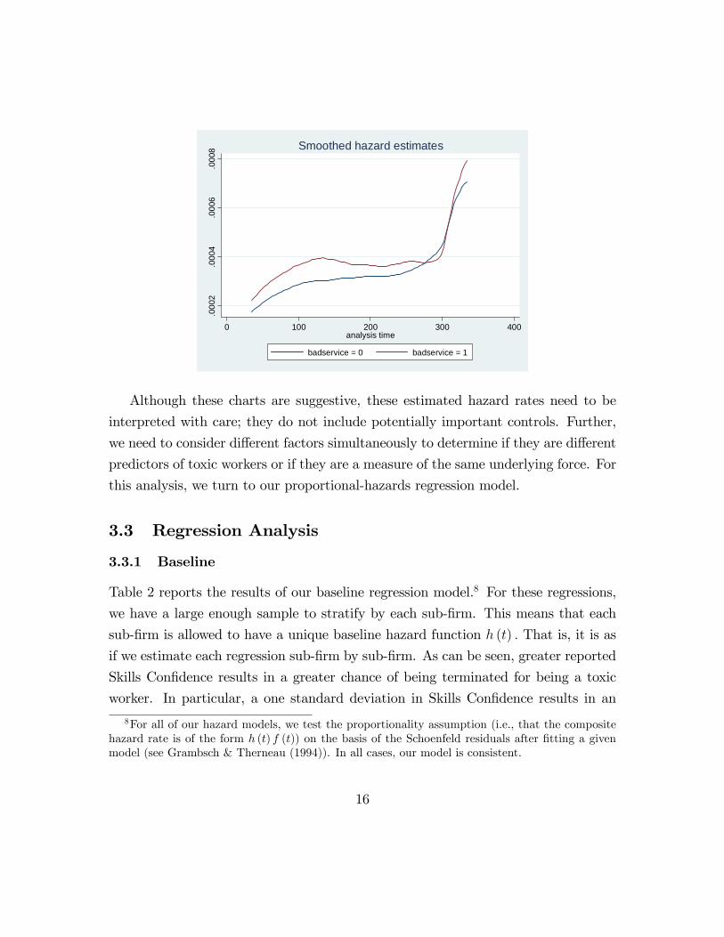
Finally, we compare the hazard rates of those with poor service orientation versus

others. As can be seen, having a poor service orientation makes one more likely to

be terminated for toxicity. If a worker that has a poor service orientation is not

terminated for toxicity in the first year, thereafter their chance of termination for

toxicity is more similar to other workers. It could be that those workers with poor

service orientation that also engage in toxicity are largely eliminated from the worker

pool by this time.

15

.000

2.0

004

.000

6.0

008


badservice = 0 badservice = 1


Although these charts are suggestive, these estimated hazard rates need to be

interpreted with care; they do not include potentially important controls. Further,

we need to consider different factors simultaneously to determine if they are different

predictors of toxic workers or if they are a measure of the same underlying force. For

this analysis, we turn to our proportional-hazards regression model.

3.3 Regression Analysis

3.3.1 Baseline

Table 2 reports the results of our baseline regression model.8 For these regressions,

we have a large enough sample to stratify by each sub-firm. This means that each

sub-firm is allowed to have a unique baseline hazard function h (t) . That is, it is as

if we estimate each regression sub-firm by sub-firm. As can be seen, greater reported

Skills Confidence results in a greater chance of being terminated for being a toxic

worker. In particular, a one standard deviation in Skills Confidence results in an

8For all of our hazard models, we test the proportionality assumption (i.e., that the compositehazard rate is of the form h (t) f (t)) on the basis of the Schoenfeld residuals after fitting a givenmodel (see Grambsch & Therneau (1994)). In all cases, our model is consistent.

16

approximate 15%9 increase in the hazard. That is, conditional on a worker not yet

having been terminated as a toxic worker, a one standard deviation increase in Skills

Confidence means that there is some 15% greater hazard of termination due to toxic

behavior. Similarly, those that have a poor service-orientation, have more than a

22% increased hazard of toxic termination. If a worker reports that she believes

rules are made to be followed (as opposed to stating that it is sometimes necessary

to break the rules to accomplish something), she has about 25% greater hazard of

being terminated for actually breaking the rules. Finally, a worker that has a one

standard deviation increase in exposure to toxic workers himself experiences a 46%

increased hazard in being terminated for engaging in toxic behavior.

If we categorize the first four columns as measures of the person and the last two

columns (including particular job type) as measures of the situation, we can state

what fraction of a toxic worker’s origin is attributable to the person versus the situ-

ation. In particular, using McFadden’s pseudo R2, we calculate that approximately

70% of the explanatory power of the model beyond a model with only an intercept

comes from the person, and the balance (i.e., 30%) from the situation. If each vari-

able in each column mattered equally, we would expect the person to explain 2/3 of

outcome (i.e., 4 out of 6). In the next section, when we only analyze a worker’s first

placement, we find from using McFadden’s pseudo R2 that person explains almost

88% of the outcome. In short, at least in our setting, there is important explanatory

power in simply knowing the person, though the situation certainly matters too, and

it seems to matter more over time.

Since we can only measure those cases of toxicity that are discovered and elim-

inated through termination, we could be only partially measuring outcomes. For

the kinds of toxic behavior that we’re studying (e.g., extreme levels such as sexual

harassment and workplace violence) it seems likely that when such behavior is ex-

hibited, discovery and termination will usually occur. However, in principle, it could

be that cleverer people are better at somehow hiding their behaviors. To explore this

9Recall that to convert estimates into a hazard ratio, simply raise e to the coeffi cient value. Forexample, a coeffi cient value of .5 results in e.5 ' 1.65. This means a one unit change in the regressoramounts to a 65% increase in the hazard ratio. Alternatively, a one standard deviation increase,when such standard deviation is .225, results in a roughly 14.6% increase in the hazard ratio.

17

possibility, we were able to obtain the results of two cognitive tests that applicants

take. These tests represents two questions, each quantitatively based with an objec-

tive correct answer. Table 3 reports the results of adding these two measures to our

previous analysis. In doing so, we found that our previous estimates are very similar

and that the cognitive test results do not explain the likelihood of toxic terminations.

In fact, one test has a positive coeffi cient point estimate and the other test has a

negative one, though neither is significant.

Ideally, we would like to conduct our analysis after randomly allocating all workers

to workgroups and then observing their experiences and performance over time.

Doing so would average out possible confounds for which it is diffi cult to control.

For example, perhaps a particular workgroup is better (or worse) at detecting and

eliminating toxic workers. However, based on discussions with company executives,

conditional on a given sub-firm, a worker’s first placement tends to be essentially

random. Exactly where an employee is initially placed depends on a variety of

factors outside the control of the worker and the workgroup in which she is placed.

For example, the work flow of a particular operation, demand and supply shocks,

and exactly when a worker turns up looking for a job are all factors determining

to which group a new hire will be assigned. Further, a workgroup supervisor does

not generally choose her group’s new worker, so the supervisor does not observe the

new worker’s predicted job fit and other individual characteristic covariates that we

use in our analysis. However, a worker’s second placement may not be essentially

random. Thus, for a robustness test, we now redo our above analysis, but only for a

worker’s first placement.

3.3.2 First Placement Only

Table 4 reports an analysis based only on an employee’s first placement. As can be

seen, the results are broadly similar to the case in which all worker placements are

included. Upon closer inspection, we see that the magnitude of the coeffi cient of

the toxic worker density is about 20% smaller. One possible explanation for this is

that the exposure to toxic workers has a cumulative effect: the same exposure over

18

a greater period of time has a greater adverse effect on a worker.

In principle, we can test statistically whether a placement is different from ran-

dom. One common method includes comparing covariates across treatments, where

treatments normally total two. However, in our setting, a "treatment" is the ini-

tial placement in each workgroup, which amounts to 2, 882 treatments, making a

comparison cumbersome. Further, one can only consider relationships pair-by-pair.

However, another common method that also allows the covariates to be interdepen-

dent is using a logit or probit model to predict treatment. Of course, this method

only works when there are two different treatments; again, we have 2, 882 treatments.

However, we can analyze a multinomial equivalent where each outcome is considered

an unordered outcome of being placed in a given workgroup. We need suffi cient

observations in order to estimate how each covariate contributes to the likelihood of

being placed in a particular workgroup. In the end, we can estimate how covariates

predict 985 workgroup placements.

The following table reports the results of these regressions.

Low Service Skills Rules: Rules:Orientation Confidence Sometimes Break Prefer Adventure

Number of Workgroups Significant at 5% 47 113 50 101Fraction of Estimated Workgroups (985) 4.77% 11.47% 5.08% 10.25%Fraction of All Workgroups (2,882) 1.63% 3.92% 1.73% 3.50%

We find that in 47 of the 985 cases Bad Job fit predicts in which workgroup a

worker is placed in, which represents almost 5% of workgroups. Skills Confidence

is significant over 11% of the time, whereas Rules covariates are significant at 5%

and 10% of the time, respectively. If all placements were generated at random, we

would expect each covariate to be significant at the 5% level, 5% of the time, on

average. When we consider the full dataset we are using to estimate effects in our

main analysis, covariates are only significant less than 3% of the time, on average.

The reason we cannot estimate covariate effects on the entire dataset of workgroups

is that generally there are too few observations for a particular workgroup, which

also means we do no expect such workgroups to create statistical aberrations on their

19

own.

We ran an additional robustness test to explicitly control for a employee’s work-

group during her first placement. In particular, we run a linear panel model with

workgroup fixed effects for a worker’s first placement.10 Here, we collapse the ex-

posure to toxic workers as an average exposure over the placement, whereas before

this was the current-period exposure. Results are reported in Table 5. The findings

with this linear model are very similar in terms of significance and magnitude when

compared with our hazard models, with the exception of the effect of Toxic exposure

. In terms of magnitudes, a worker that is predicted to have Low Service Orientation

has an additional .9% chance of becoming a terminated toxic worker, which is an

increase of 20% from the baseline toxic worker rate of 4.5%. A one standard deviation

in Skills Confidence results in a roughly 11% chance of becoming a terminated toxic

worker. Those who state that rules should never be broken are 20% more likely to

be terminated for toxic behavior. A one standard deviation increase in exposure to

other toxic workers induces a roughly 98% increased chance of a worker becoming a

toxic worker. Finally, In short, these effects are consistent with those found with our

previous models.

3.3.3 Toxic Worker Performance

For a subset of the data, we have performance data on the workers. For this group,

as discussed in section 3.1, we have a measure of each employee’s time to produce

one unit of quantity and a measure of their quality of work. We then use this data

to calculate a worker-specific fixed effect of each of these measures, which we refer

to as Performance Quantity Time FE and Performance Quality FE, respectively.

Looking simply at mean FE values, we find that the average Performance Quan-

tity Time FE is less for those ultimately fired for toxicity than those that are not

toxic (t-test with unequal variance yields a p-value= .0376). That is, toxic workers

are more productive than those that are not ultimately terminated for toxicity. When

10Note that we do not control for position type in these specifications. A particular workgrouptypically consists of the same set of position types, and thus the variance matrix naturally becomesunusable when we do attempt to control for position type simultaneously with workgroup.

20

we consider Performance Quality FE, we find that toxic workers have lesser quality

than non-toxic workers; however, results do not quite reach conventional levels of

statistical significance (p-value= .1233). Of course these are simply means and we

should consider analysis with controls. In particular, we need to relate the produc-

tivity of workers and whether or not that worker is terminated for toxic behavior

while controlling for the previous factors that are important for identifying toxicity.

Table 6 reports the results of introducing these additional measures to our original

analysis reported in Table 2. The other variables of interest previously studied are

qualitatively the same as in table 2, although the levels of significance are diminished

for this considerably smaller sample size.

Similar to our findings of comparing the means, those who are terminated for

engaging in toxic behavior are more productive than non-toxic employees; equiva-

lently, those who are slower (i.e., large values of Performance Quantity Time FE)

are less likely to be toxic. In terms of magnitude, a one standard deviation in time

per unit of production results in a 56% reduction in the hazard of becoming a toxic

worker. However, those workers with poorer quality performance are more likely to

be toxic. Here, a one standard deviation increase in the quality of production results

in a 27% decrease in the hazard. With controls, this relationship is not significant

at conventional levels.

It might seem that toxic workers are simply those that trade work quality for

speed and those workers that produce higher quality must also be slower workers.

However, this is not the case. Clearly, there is a natural tradeoff between speed and

quality of work. Yet, there are almost 50% more workers that produce high quality

work quickly (32.4% of workers) than those that produce low quality work quickly

(23% of workers). Thus, although toxic workers are quicker than the average worker,

they are not necessarily more productive in a quality-adjusted sense. In the long run,

these kinds of workers are not likely to improve overall organizational performance.

Finding Superstars vs. Losing Toxic Workers With performance data we

can also compare the strategy of finding a "superstar" worker versus avoiding a toxic

one. As discussed in the introduction, many firms, as well as the extant literature are

21

focused on finding and keeping the next star performer, whereas much less attention

is devoted to avoiding toxic workers. Given a firm with limited resources, which

strategy is more fruitful? Although we certainly cannot answer this question for all

possible settings, we can asses this trade-off for our setting.

To generate a straightforward comparison of the value of each of these focuses,

we quantify the value of a star performer by identifying the cost savings from her

increased output level. That is, without such a star performer, a firm would have

to hire additional workers to achieve the same output they enjoy when they have a

superstar. In the table below, the column "Hire a Superstar" reports the cost saving

based on the top 1%, 5%, 10%, and 25% performers. We calculate the percent in

increased performance for each of these performance levels and multiply it by the

average worker salary, based on company records. This is an upper bound of the cost-

savings from hiring a Superstar since increased performance is often accompanied by

increased wages.

For comparison, we report in the "Avoid a Toxic Worker" column the induced

turnover cost of a toxic worker, based on company figures. Induced turnover cost

captures the expense of replacing additional workers lost in response to the presence

of a toxic worker on a team. The total estimated cost is $12,489 and does not include

other potential costs, such as litigation, regulatory penalty, and reduced employee

morale. Also not included are the secondary costs of turnover that come from a

new worker’s learning curve: a time of lower productivity precedes a return to higher

productivity. Thus, this estimate is likely a lower bound on the average cost of a

toxic worker, at least for this empirical setting.

Hire a Avoid aSuperstar Rank Superstar Toxic Worker

top 25% $ 1,951 $ 12,489top 10% $ 3,251 $ 12,489top 5% $ 3,875 $ 12,489top 1% $ 5,303 $ 12,489

Costsavings

22

In comparing the two costs, even if a firm could replace an average worker with

one who performs in the top 1%, it would still be better off by replacing a toxic

worker with an average worker by more than two-to-one. That is, avoiding a toxic

worker (or converting them to an average worker) provides more benefit than finding

and retaining a superstar. Assuming that it is no more costly to avoid a toxic

worker (or replace them with an average worker) than it is to find, hire, and retain

a superstar, it is also more profitable to do the former over the latter. Of course,

this differential between the superstar and toxic worker might not be as drastic in

other settings. Nonetheless, finding a top 1% worker can be both diffi cult and costly.

Further, sometimes "stars" that hiring managers discover via another firm are not

able to transport their same elevated level of productivity to their next employer

(Groysberg (2012)). Finally, as some high-stakes finance workers recently showed

us leading up to the Great Recession, high-flying lines of work can generate both

superstars and toxic workers with enormous impacts.

4 Discussion

Based on our analysis, we have a variety of takeaways for managers. From our

study, it seems clear that toxic workers originate both as a function of preexisting

characteristics and the environment in which they work. In particular, we found

consistent evidence that those who seem overconfident in their abilities, who are

poorly service-oriented, and who claim rules should be followed, are more likely to

become toxic workers and break the rules. One strategy for hiring managers is to

screen potential workers for these traits to reduce the chance of hiring toxic workers.

Of course, there are more dimensions to a good (and bad) hire beyond whether

or not candidates have a higher propensity to become toxic. Worker productivity

is also important. Interestingly, we found that toxic workers are apparently more

productive, at least in terms of the quantity of output. This could also explain how

toxic workers are able to remain in an organization for as long as they do. For

example, an investment bank with a rogue trader who is making the firm millions

in profits might be tempted to look the other way when the trader is found to be

23

overstepping the rules. Pierce and Snyder (2013) find unethical workers enjoy longer

tenures. However, we also found evidence that the quality of production for these

workers is lower. This means that eventually, the value of the higher productivity

will be diminished, perhaps drastically, as the consequences of lower-quality work

are manifested.

This performance finding suggests that toxic workers are similar to what Jack

Welch described as "Type 4" workers– those that deliver on the numbers but do

not have the right values. Welch claimed that while diffi cult to do, it was critical

to remove such workers: "People are removed for having the wrong values...we don’t

even talk about the numbers" (Bartlett and Wozny (2005)). Thus, we find evidence

that such a policy– one that removes the "big shots" and "tyrants" seems to be one

that would lead to more productive organizations in general.11 Similarly, Delong and

Vijayaraghavan (2003) argue that the top performers are not always the best workers

to pursue over even the average worker, as the former can also create organizational

issues, including reckless behavior.

Although we do find certain preexisting traits that predict toxic workers, this does

not mean that those traits were always present in the worker. Though it is beyond

the scope of this paper, it would be interesting to learn to what extent work-life

experiences breed the preexisting traits that we have found to lead to toxic workers.

It would be very valuable to discover what firms can currently do to limit the chances

of converting a "normal" worker to a future toxic worker.

In this vein, we did find that a worker’s environment also substantially influenced

her propensity to become a toxic worker. We documented that holding a particular

type of position, as well as exposure to other toxic workers negatively influenced the

likelihood of one becoming toxic. Hence, this suggests that managing toxic workers

is not simply a matter of screening them out of the firm, but also minding the work

environment.11We thank Tarun Khanna for this Jack Welch example.

24

5 Conclusion

In the end, a good or bad hiring decision is multidimensional (Lazear & Oyer (2007)

and Hermalin (2013)). We have identified several personality and situational factors

that lead to a worker engaging in objective toxic behavior. Knowledge of these

factors can be used to better manage for toxic workers. We have also discovered some

important effects of toxic workers. However, there are surely additional traits that

could be used to identify toxic workers. Similarly, it would be helpful to know which

other environmental factors nudge an otherwise normal worker towards becoming a

toxic worker and possibly creating the preexisting workplace conditions that lead to

toxic behavior. Future research can shed light on these questions. This latter focus

seems particularly important, because to the extent that we can reduce a worker’s

propensity to become toxic, we are helping not only the firm, but the worker himself,

those around him, and the potential firms where that employee may work in the

future. Since we found some evidence that a toxic worker can have more impact on

performance than a "superstar," it may be that spending more time limiting negative

impacts on an organization might improve everyone’s outcome to a greater extent

than only focusing on increasing positive impacts. We have taken a first step in

exploring this notion and hope that we witness future progress in this area.

25

References

[1] Andreoni, J. and J. Miller (2002) “Giving According to GARP: An Experimental

Test of the Consistency of Preferences for Altruism,”Econometrica, 70 (2), 737-

753.

[2] Azoulay, P., Graff Zivin, J., & Wang, J. (2010). Superstar Extinction. The

Quarterly Journal of Economics, 125(2), 549-589.

[3] Banerjee, A., Mullainathan, S., & Hanna, R. (2012). Corruption (No. w17968).

National Bureau of Economic Research.

[4] Bartlett, C.A., & Wozny, M. (2005). GE’s Two-Deade Transformation: Jack

Welch’s Leadership. HBS 9-399-150. Boston: Havard Business School Publishing,

2005.

[5] Baumeister, R. F., Bratslavsky, E., Finkenauer, C., & Vohs, K. D. (2001). Bad

is stronger than good. Review of General Psychology, 5(4), 323.

[6] Bertrand, M., & Mullainathan, S. (2001). Do people mean what they say? Im-

plications for subjective survey data. American Economic Review, 67-72.

[7] Cameron, A. C., & Trivedi, P. K. (2005). Microeconometrics: methods and

applications. Cambridge university press.

[8] Delong, T. J., & Vijayaraghavan, V. (2003). Let’s hear it for B players. Harvard

Business Review, 81(6), 96-102.

[9] Derfler-Rozin, R., Moore, C., & Staats BR. (2015). Enhancing ethical behavior

through task variety. London Business School working paper.

[10] Ermongkonchai, P. (2010). Understanding Reasons for Employee Unethical Con-

duct in Thai Organizations: A Qualitative Inquiry, Contemporary Management

Research, 6(2), 125-140.

26

[11] Estes, Z., & Adelman, J. (2008). Automatic vigilance for negative words in

lexical decision and naming: Comment on Larsen, Mercer, and Balota (2006).

Emotion, 8(4), 441-444.

[12] Fisman, R., S. Kariv, and D. Markovits (2007) “Individual Preferences for Giv-

ing,”American Economic Review, 97 (5), 1858—1876.

[13] Ford, R. C., & Richardson, W. D. (1994). Ethical decision making: A review of

the empirical literature. Journal of Business Ethics, 13(3), 205-221.

[14] Frank, D. H., & Obloj, T. (2014). Firm-specific human capital, organizational

incentives, and agency costs: Evidence from retail banking. Strategic Manage-

ment Journal, 35(9), 1279-1301.

[15] Gibbons, R., & Roberts, J. (Eds.). (2013). The Handbook of Organizational

Economics. Princeton University Press.

[16] Gino, F., & Ariely, D. (2012). The dark side of creativity: original thinkers can

be more dishonest. Journal of Personality and Social Psychology, 102(3), 445.

[17] Grambsch, P. M., & Therneau, T. M. (1994). Proportional hazards tests and

diagnostics based on weighted residuals. Biometrika, 81(3), 515-526.

[18] Greenberg, J. (2002). Who stole the money, and when? Individual and situ-

ational determinants of employee theft. Organizational Behavior and Human

Decision Processes, 89(1), 985-1003.

[19] Greve, H. R., Palmer, D., & Pozner, J. E. (2010). Organizations gone wild: The

causes, processes, and consequences of organizational misconduct. The Academy

of Management Annals, 4(1), 53-107.

[20] Groysberg, B. (2012). Chasing stars: The myth of talent and the portability of

performance. Princeton University Press.

[21] Hermalin, B. (2013). Leadership and corporate culture. Handbook of Organiza-

tional Economics, 432-478.

27

[22] Larkin, I. (2014). The cost of high-powered incentives: Employee gaming in

enterprise software sales. Journal of Labor Economics, 32(2), 199-227.

[23] Lazear, E. P., & Oyer, P. (2007). Personnel economics (No. w13480). National

Bureau of Economic Research.

[24] Litzky, B. E., Eddleston, K. A., & Kidder, D. L. (2006). The good, the bad, and

the misguided: How managers inadvertently encourage deviant behaviors. The

Academy of Management Perspectives, 20(1), 91-103.

[25] Loe, T. W., Ferrell, L., & Mansfield, P. (2000). A review of empirical studies

assessing ethical decision making in business. Journal of Business Ethics, 25(3),

185-204.

[26] MacLean, T. L., & Behnam, M. (2010). The dangers of decoupling: The relation-

ship between compliance programs, legitimacy perceptions, and institutionalized

misconduct. Academy of Management Journal, 53(6), 1499-1520.

[27] Minor, D. (2014). Shadow risks and disasters. Kellogg School of Management,

working paper.

[28] F. Oberholzer-Gee & Wulf, J. (2012). Incentives-based misconduct: Earnings

Management from the Bottom Up: An Analysis of Managerial Incentives Below

the CEO. HBS Working Paper 12-056.

[29] Oettl, A. (2012). Reconceptualizing stars: Scientist helpfulness and peer perfor-

mance. Management Science, 58(6), 1122-1140.

[30] Petit, V., & Bollaert, H. (2012). Flying too close to the sun? Hubris among

CEOs and how to prevent it. Journal of Business Ethics, 108(3), 265-283.

[31] Pierce, L., & Balasubramanian, P. (2015). Behavioral field evidence on psy-

chological and social factors in dishonesty and misconduct. Current Opinion in

Psychology, 6, 70-76.

28

[32] Pierce, L., & Snyder, J. (2008). Ethical spillovers in firms: Evidence from vehicle

emissions testing. Management Science, 54(11), 1891-1903.

[33] Pierce, L., & Snyder, J. A. (2013). Unethical demand and employee turnover.

Journal of Business Ethics, 1-17.

[34] Roberts, J., & G. Saloner. (2013). Strategy and Organization. Handbook of

Organizational Economics, 799-854.

[35] Robinson, S. L., & Bennett, R. J. (1995). A typology of deviant workplace

behaviors: A multidimensional scaling study. Academy of management journal,

38(2), 555-572.

[36] Sauermann, H., & Cohen, W. M. (2010). What makes them tick? Employee

motives and firm innovation. Management Science, 56(12), 2134-2153.

[37] Tenbrunsel, A. E., & Smith-Crowe, K. (2008). 13 Ethical Decision Making:

Where We’ve Been and Where We’re Going. The Academy of Management

Annals, 2(1), 545-607.

[38] Trevino, L. K. (1986). Ethical decision making in organizations: A person-

situation interactionist model. Academy of management Review, 11(3), 601-617.

[39] Tversky, A., & Kahneman, D. (1992). Advances in prospect theory: Cumu-

lative representation of uncertainty. Journal of Risk and Uncertainty J Risk

Uncertainty, 5(4), 297-323

[40] Vardi, Y. (2001). The effects of organizational and ethical climates on miscon-

duct at work. Journal of Business Ethics, 29(4), 325-337.

[41] Weaver, G. R., & Trevino, L. K. (1999). Compliance and Values Oriented Ethics

Programs. Business Ethics Quarterly, 9(2), 315-335.

29

Table 1: Summary Statistics

Variable Obs Mean Std. Dev. Min MaxLow Service Orientation 248370 0.15 0.35 0.00 1.00Skills Confidence Level 248370 -0.01 0.23 -0.24 0.92Rules: Sometimes Break Them 248370 0.14 0.34 0.00 1.00Rules: Prefer Adventure 248370 0.44 0.50 0.00 1.00Density of Toxic Workers 248370 0.04 0.04 0.00 0.80Performance Quantity Time FE 62618 -32.77 213.11 -462.94 1488.31Performance Quality FE 20089 -0.05 0.13 -0.91 0.23Terminated for Toxic Behavior 248370 0.01 0.10 0 1

Table 2: Terminations as a Function of Worker Type and Environment

(All Placements)

Worker and Environment (1) (2) (3) (4) (5) (6)Low Service Orientation 0.2808*** 0.2090*** 0.2077*** 0.2047*** 0.2030*** 0.2023***

(5.30) (3.81) (3.78) (3.71) (3.69) (3.68)

Skills Confidence Level 0.5215*** 0.5206*** 0.5177*** 0.5033*** 0.5034***(6.42) (6.41) (6.36) (6.18) (6.17)

Rules: Sometimes Break Them -0.2373*** -0.2284*** -0.2247*** -0.2272***(-3.75) (-3.55) (-3.49) (-3.53)

Rules: Prefer Adventure -0.0274 -0.0193 -0.0184(-0.67) (-0.47) (-0.45)

Density of Toxic Workers 2.5581*** 2.5182***(11.74) (11.49)

Position Controls No No No No No Yes

Log Likelihood -18446.4880 -18427.3077 -18419.9216 -18419.6990 -18372.5281 -18368.2087

N 246599 246599 246599 246599 246599 246599

Cox proportional hazard model used for estimationNon parametric hazard functions estimated at the sub-firm level

Z scores reported in parentheses based on standard errors clustered at the worker level* p<0.10, ** p<0.05, *** p<.01

Outcome: Terminated Toxic Worker

Table 3: Cognitive Scores and Terminations

(All Placements)

Worker and Environment (1) (2) (3) (4) (5) (6)Cognitive Test I Correct 0.0051 0.0164 0.0200 0.0201 0.0304 0.0258

(0.10) (0.32) (0.39) (0.39) (0.59) (0.50)

Cognitive Test II Correct -0.1092* -0.0777 -0.0708 -0.0693 -0.0581 -0.0599(-1.76) (-1.25) (-1.14) (-1.11) (-0.93) (-0.96)

Low Service Orientation 0.2730*** 0.2051*** 0.2043*** 0.2015*** 0.2004*** 0.1996***(5.12) (3.73) (3.71) (3.65) (3.64) (3.63)



Rules: Prefer Adventure -0.0257 -0.0180 -0.0169(-0.63) (-0.44) (-0.41)



Log Likelihood -18444.8609 -18426.5004 -18419.2375 -18419.0419 -18371.9870 -18367.6758

N 246599 246599 246599 246599 246599 246599




Table 4: Terminations as a Function of Worker Type and Environment

(First Placements Only)

Worker and Environment (1) (2) (3) (4) (5) (6)Low Service Orientation 0.3279*** 0.2617*** 0.2608*** 0.2638*** 0.2595*** 0.2597***

(5.66) (4.35) (4.33) (4.37) (4.30) (4.30)



Rules: Prefer Adventure 0.0272 0.0311 0.0300(0.59) (0.67) (0.65)



Log Likelihood -13661.0461 -13649.4261 -13644.9028 -13644.7302 -13627.5793 -13626.9476

N 190178 190178 190178 190178 190178 190178




Table 5: Linear Model of Terminations with Workgroup Fixed Effects

(First Placements Only)

Worker and Environment (1) (2) (3) (4) (5)Low Service Orientation 0.0128*** 0.0093*** 0.0093*** 0.0097*** 0.0091***

(4.04) (2.86) (2.87) (2.96) (2.82)

Skills Confidence Level 0.0243*** 0.0243*** 0.0246*** 0.0208***(5.07) (5.06) (5.11) (4.39)

Rules: Sometimes Break Them -0.0074*** -0.0083*** -0.0076***(-2.74) (-3.01) (-2.79)

Rules: Prefer Adventure 0.0028 0.0025(1.33) (1.23)

Avg Density of Toxic Workers 1.1078***(20.70)

R Squared 0.044 0.044 0.044 0.045 0.070Adjusted R Squared 0.022 0.023 0.023 0.023 0.049

N 44710 44710 44710 44710 44710


t statistics reported in parentheses based on standard errors clustered at the workgroup level* p<0.10, ** p<0.05, *** p<.01

Table 6: Terminations with Worker Performance

(All Placements)

Worker and Environment (1) (2) (3)Performance Quantity Time FE -0.0036*** -0.0039***

(-6.79) (-5.33)

Performance Quality FE -2.1925*** -2.4419***(-4.90) (-5.28)

Low Service Orientation 0.0383 -0.0620 -0.0853(0.41) (-0.41) (-0.55)

Skills Confidence Level 0.4069*** 0.4597** 0.4686**(2.93) (2.50) (2.54)

Rules: Sometimes Break Them -0.0215 -0.0226 0.0192(-0.20) (-0.14) (0.12)

Rules: Prefer Adventure -0.0823 -0.2627*** -0.2449**(-1.17) (-2.64) (-2.44)

Density of Toxic Workers 1.5359*** 1.7591*** 1.5971***(5.21) (5.83) (5.15)

Position Controls Yes Yes yes

Log Likelihood -5859.5624 -3233.1108 -3165.6394

N 62419 19983 19751


Cox proportional hazard model used for estimationNon parmetric hazard functions estimated at the sub-firm level

Z scores reported in parentheses are based

* p<0.10, ** p<0.05, *** p<.01on standard errors clustered at the worker level

toxic workers - harvard university

Documents