TPOS 2020 ProjectReview and re-design the Tropical Pacific Observing System

– Rethink in response to new needs, purposes, challenges: Define requirements– Renew the interagency and intergovernmental cooperation that has been the

hallmark of the TPOS since the mid-1980’s– Take advantage of new science and technology

1

Today’s outline:– Overview of the project (15 mins)– Recommended process studies (15 mins)– Discussion!!!

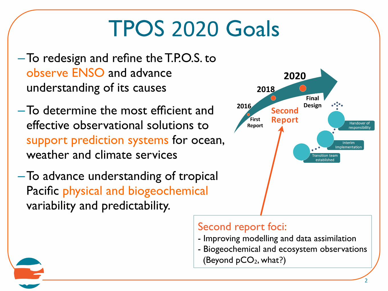
TPOS 2020 Goals–To redesign and refine the T.P.O.S. to

observe ENSO and advance understanding of its causes

–To determine the most efficient and effective observational solutions to support prediction systems for ocean, weather and climate services

–To advance understanding of tropical Pacific physical and biogeochemical variability and predictability.

2

SecondReport

Second report foci:- Improving modelling and data assimilation- Biogeochemical and ecosystem observations (Beyond pCO2, what?)

An integrated view• Complementary “backbone” technologies:

– Satellites give global coverage, fine horizontal detail)

– Moorings sample across timescales, allow co-located ocean-atmosphere observations, velocity sampling

– Argo resolves fine vertical structure, adds salinity, maps subsurface T and S and connects to subtropics

• New scientific understanding and issues:– Role of high-frequencies, especially the diurnal cycle

– Focus on the coupled boundary layers

– Physical-biogeochemical connections and impacts

Assimilating models integrate diverse observations

→ Users will increasingly rely on gridded products

3

4

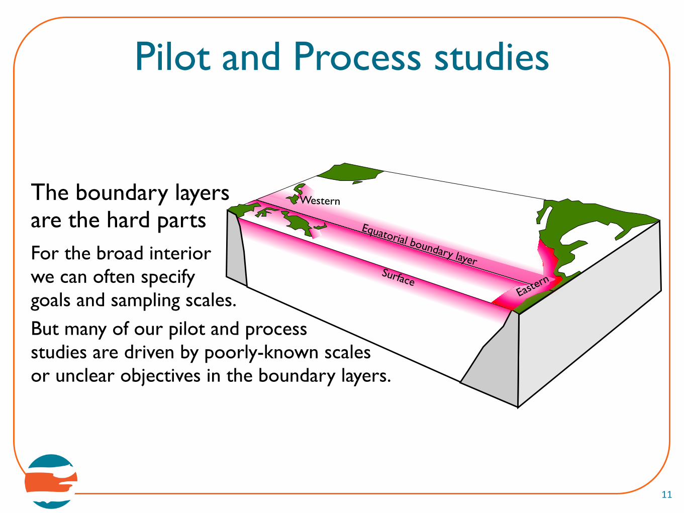
We view the tropical Pacific as consisting of a broad interiorplus four “boundary layers”:

Surface, Equatorial, Eastern and Western

Equatorial boundary layerSurface

Eastern

WesternThe boundary layersare the hard partsIn an integrated systemthat includes satellites,we are less tied to a gridand can focus in situ sampling on key regimes.

Requirements for the backboneWhat drives our recommendations?  

Example: Vector winds

5

QuikSCAT rain-flag frequency during 1999-2009. Over much of the Pacific ~25% of QuikSCAT samples are flagged as potentially invalid due to rain.

This does not mean that scatterometer winds are unusable under rain, but they are in question.It is also true that wind products from different centers differ significantly.

The global climate is exquisitely sensitive to the equatorial zonal wind, so we must get this right.

First Report of TPOS 2020

34

constraint. NWP and atmospheric reanalysis systems assimilate scatterometer backscatter using a

transfer function for wind that ignores surface current effects. In the tropics, surface currents can be

strong and winds relatively weak. Therefore, estimation of wind stress and its curl using absolute winds

requires a correction of the surface current effects; otherwise, it can result in misleading constraints for

ocean/atmosphere models. Therefore, neglect of the ocean surface velocity on wind stress estimation can

degrade wind products. Measurements of near-surface currents (see section 3.1.3.2), with high

spatiotemporal resolution (at least at all wind calibration sites) would facilitate comparison and synthesis

of relative winds obtained from scatterometers with absolute winds derived from buoys and NWP models.

Wind measurements derived from satellite scatterometers have demonstrated good consistency with

wind measurements obtained from moorings, with an average RMS difference (between satellite and

mooring winds) of approximately 1 m s-1 (Figure 3-2). This does not reflect only the uncertainty of the

satellite wind measurements, but also contributed by a number of other factors. These factors include the

uncertainty of the mooring winds, the scale-mismatch between satellite and mooring measurements (i.e.,

averages within satellite footprint versus point-wise measurements). However, the limited sampling by

satellites cause sampling errors that affect satellite-derived gridded wind products (Figure 3-3) and the

differences of these products from mooring winds that can be more substantial than the uncertainty of

the satellite measurement per se. It is important not to confuse the measurement error with the sampling

error. Increasing satellite coverage with a variety of orbits to capture diurnal variability can alleviate the

sampling errors. Since the 2000s, the coverage of the ocean by scatterometers is approximately 60% at

the 6-hourly interval (Atlas et al., 2011). An enhancement of coverage from 60% to 90% at the 6-hourly

interval can provide a much more adequate constraint on estimates from NWP models and from

synthesized wind products.

Figure 3-2: Satellite wind speeds compared with collocated buoy measurements, separated for all-weather, rain-free, and

raining conditions: (top row) Binned satellite wind speeds as functions of buoy speed; (bottom row) RMS wind speed difference

between satellite and buoys as a function of buoy wind speed. Each column represents one of the four satellite instruments

considered in this analysis. Courtesy of Larry O’Neill.

TAO was originally designed to map winds, before scatterometry. Now we propose to reduce buoy locations, relying more on scatterometer winds.

Two distinct issues:1) How well do scatterometers measure winds themselves?

Winds with a reduced moored array

8

Extensive investigation:- Only a few ongoing cal/val points are needed in the tropics- Specific regions need in situ referencing (heavy rain / low winds)- Equator needs referencing between satellite generations

These considerations were influential in shaping our design:In situ wind sampling in heavy rain regimes: ITCZ, SPCZ, Warm poolMaintain full sampling along the equator

2) How well do present analyses produce credible wind fields? The mapping issues are more difficult:Products from different centers differ considerably! Work is needed!

TPOS 2020 must provide the in situ observations for adequate referencing of scatterometer winds as wind-gridding improves

The First Report• Published 30 December 2016 (ref. GCOS-200)• 22 Recommendations• 15 Actions• First published design following the GOOS Framework• 2 rounds of review and revision

7

tpos2020.org/first-­‐report(much  of  this  applies  to  the  other  tropical  oceans!)

xxx

xx

xxx

x

x

xxxx

TAO

Currentmeter

TRITON

x RemovedTRITON

Light-blue shading = Standard (3°x3°) Argo

New SOA (TBD) Added TAO

New SOA

TAO

Added CM

RemovedTAO

TRITON

Future TAO + JAMSTEC + SOA arrays

Present/historical TAO −TRITON array

Dark blue = Double Argo

Specific Recommendations

8

• Double Argo within 10°S-10°N • Reconfigure the moored array

Only 3 TRITONsites remain

More-capable moorings, targeting:

the equatorial circulation, the mixed layer, its interaction with the atmosphere, key regimes

Proposedeventual in situ

“backbone”

The climate record in an evolving observing system

A “climate data record” is a time series at a point (examples).

A “climate record” is a set of measurements that enable detection and accurate description of an element of climate variability in its longterm context.

Barrier layer thickness (Argo)

Salinity at 0°,156°E (TRITON)

9

Conclude overview: Successes, challenges

• Large amount of talent, thought, interest

• Concrete redesign proposed

• Strong endorsement by sponsors (US and international)Already considerable investment underway

• Risks of change:- We will live with the new design for O(decade) ... hard to guess future needs. Where are the models going? Where are the data assimilation systems going?- In a world of sparse funding, how do we avoid damaging the climate record?Requires process studies (rest of session)

10

Pilot and Process studies

11

Equatorial boundary layerSurface

Eastern

WesternThe boundary layersare the hard partsFor the broad interiorwe can often specifygoals and sampling scales.But many of our pilot and processstudies are driven by poorly-known scales or unclear objectives in the boundary layers.

Criteria for TPOS 2020 process studies

• Our fundamental responsibility is to build the backbone observing system (which makes everything else possible)

• Sustained diagnoses will occur largely through model products that integrate diverse data sources, remote and in situ

12

Thus, we seek process studies that:- are explicitly coordinated with parameterization development: Must identify a path to improvement that needs specific observational guidance not available from the sustained obs (CPT model)- point towards increasing ability of models to infer the action of the process from ongoing sparser sampling, and to refinements of the sustained sampling

Proposed studies are not pre-wired! Open to everyone!Our present list is not complete or exclusive!

SaildroneWave glider

13

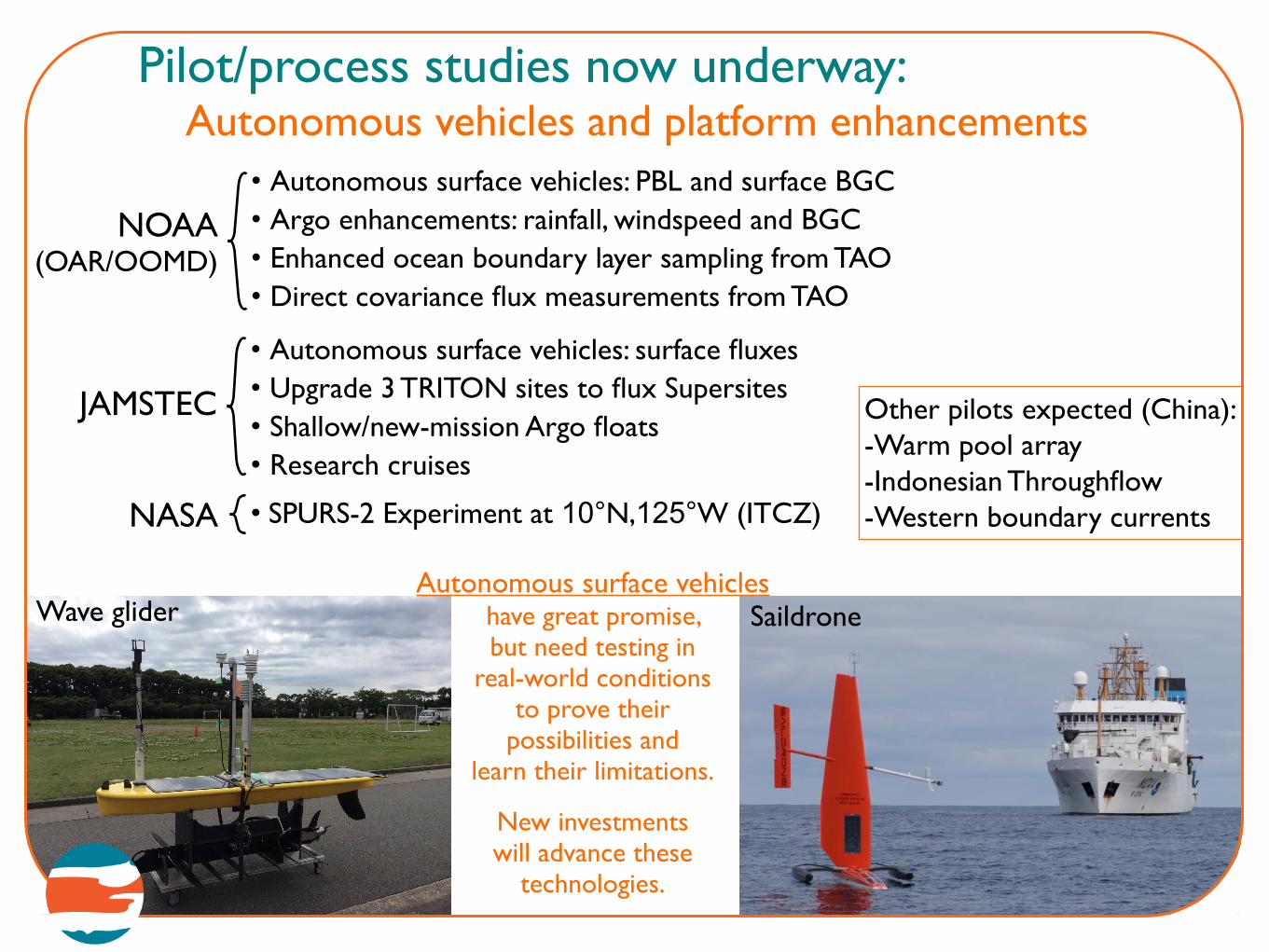
Pilot/process studies now underway:Autonomous vehicles and platform enhancements

• Autonomous surface vehicles: PBL and surface BGC• Argo enhancements: rainfall, windspeed and BGC• Enhanced ocean boundary layer sampling from TAO• Direct covariance flux measurements from TAO

NOAA(OAR/OOMD)

• Autonomous surface vehicles: surface fluxes• Upgrade 3 TRITON sites to flux Supersites• Shallow/new-mission Argo floats• Research cruises

JAMSTEC

Autonomous surface vehicleshave great promise, but need testing in

real-world conditions to prove their

possibilities and learn their limitations.

New investmentswill advance these

technologies.

Other pilots expected (China):-Warm pool array-Indonesian Throughflow-Western boundary currentsNASA • SPURS-2 Experiment at 10°N,125°W (ITCZ)

Warm Pool Edge metric

Advantages Disadvantages

SST threshold (28 - 30oC)

• Important for atmospheric response, e.g. convection, tropical cyclones, intraseasonal variability including WWBs.

• Satellite and in-situ data products readily available.

• Strongly affected by background warming • Inconsistent thresholds between models • Higher SST isotherms not always present • Decouples from other definitions in extreme

events and at high-frequency time scales (such as diurnal cycle).

SSS threshold (34.2 to 35.2)

• More closely representative of dynamical edge.

• Same as above • Limited data availability, though new satellite

products (SMOS & Aquarius) now available Maximum SSS gradient

• Insensitive to background state • Representative of dynamical edge

• Limited data availability • Noisy and may be contaminated by high

frequency variability Isotherm fit to SSS gradient

• As above. • Useful for model intercomparison

• Isotherm needs to be revised with background warming

Density threshold (not common)

• Combines temperature and salinity changes

• Incorporates disadvantages of both temperature and salinity.

Convergence using hypothetical drifters

• Representative of ‘dynamical edge’ • Can use dynamic height, or satellite mean

sea level as proxy

• Need to compute hypothetical drifters • May not converge in models due to the high

sensitivity to background mean state • Limited observations and reliance on

combined satellite estimates. Chl-a (e.g. 0.1mg/m3)

• Sharp front • Limited to satellite record • May decouple from physical parameters.

Nitrate/pCO2 • Usually tracks the frontal zone • Limited observations • May decouple from physical parameters.

Table 1. Metrics used to describe the edge of the Western Pacific Warm Pool and their advantages and disadvantages.

Figure 1. Schematic of the WPWM mean state and changes for El Nino conditions (inset)

The front at the east edge of the warm pool interacts with theatmosphere, especially during theonset of El Niño.

Critical processes in the east include the stratus/cold tongue front/ITCZ systemand coastal upwelling.

Equatorial upwelling is fundamental but poorly known; its modeling is uncertain.

Low-latitude western boundary currents and theIndonesian Throughflow are principal conduits of tropical-subtropical interaction.

The diurnal cycle can be an important mechanism allowing downward propagation of heat and momentum fluxes.

The 30-year record of surface pCO2 shows strong annual, interannual and decadal variability of CO2 fluxes in the east Pacific cold tongue.

•Pilot studies enhance TPOS capability

•Process studies to understand phenomena

•Modeling studies add value to observations, assess their impact

Advance: Research required!

Barrier layers in the west Pacific warm poolaffect the penetration of momentum fluxes.

Pilot / process studies in the First Report

15

Pilots (not discuss today?)6.1.1 Strategy/feasibility for observing LLWBCs6.1.2 Peru coastal upwelling 6.1.3 Determining time/space scales for BGC observations6.1.4 Direct measurements of air-sea fluxes6.1.5 Pilot climate observing station at Clipperton Island6.1.6 Assessing the impact of changes to the backbone6.1.7 Assessing utilization of TPOS observations

Process studies6.2.1 Equatorial upwelling and consequences6.2.2 Air-sea interaction at the northern edge of the warm pool6.2.3 Air-sea interaction at the eastern edge of the warm pool6.2.4 East Pacific ITCZ/warm pool/cold tongue/stratus complex

PUMP: Pacific Upwelling and Mixing Physics

16

The equatorial zone in the Pacific has global significance .Coupled equatorial feedbacks underlie all Pacific climate variability.Upwelling is the main driver of property emergence (heat, CO2 , ...).

At present, this circulation is almost unconstrained by observations.

Meridional and time scales are short (100km or less, hours/days) Our sampling is further from the actual scales than anything else in this region. We must teach models how to infer the action of upwelling from sparse clues.

z

y

x

Red = Solar Green = Wind Blue = Velocity = Mixing

Upwelling is O(m/day) → vertical mixing must be very strong

Equatorial boundary layer

17

Johnson et al. (2001)(Shipboard ADCP mean)

Mean zonal current (colors) and salinity (white contours) at 140°W (sketch of w)

(S-ADCP misses upper 25m)

18

CESM-POP with different horizontal resolutions (mean)1-degree 1/10-degree

(Frank Bryan)

Colors = u

Colors = w

Modern modelmeridionalcirculations

u(eq,z) nearly identical:With TAO eq currentprofiles, modelers have learned to tune this.

w quite different, as isT(eq,z):Implications for air-seainteraction diverge.Vertical circulation isnow unconstrained byobservations.Guidance needed.

Unconstrained models ....

19

MOM

Mean u and wat 0°, 140°W

Compare twoforced OGCMs:MOM2 (1/3°) vsCCSM2 (1/10°)

CCSM

CCSM (Bryan), MOM (Vecchi)

Two models withvery similar u (close to observations)but very different w

20

How to conduct an upwelling experiment?Goals:- Guide model parameterizations to represent upwelling and its consequences from sparse sustained sampling- Learn what sustained sampling is needed to allow upwelling inference: Meridional density of moorings, Argo floats- How does equatorial SST change when the wind changes?

Challenges:- w is a velocity derivative; hard to measure accurately, requires time-averaging- Fast-timescale and strong TIW variability hard to overcome- Unknown meridional scales require oversampling (expensive) (Is du/dx important? more expensive)- Ideally would include turbulence measurements, depending on model needs

Point CMsor short-range ADCPabove 50m

Blue = Present TAO, Red = Additions

100m

0°500m

2°N2°S

50m

Ticks =T-sensors

300m

1°S 1°N

Upward-looking ADCPs

Warm Pool Edge metric

Advantages Disadvantages

SST threshold (28 - 30oC)

• Important for atmospheric response, e.g. convection, tropical cyclones, intraseasonal variability including WWBs.

• Satellite and in-situ data products readily available.

• Strongly affected by background warming • Inconsistent thresholds between models • Higher SST isotherms not always present • Decouples from other definitions in extreme

events and at high-frequency time scales (such as diurnal cycle).

SSS threshold (34.2 to 35.2)

• More closely representative of dynamical edge.

• Same as above • Limited data availability, though new satellite

products (SMOS & Aquarius) now available Maximum SSS gradient

• Insensitive to background state • Representative of dynamical edge

• Limited data availability • Noisy and may be contaminated by high

frequency variability Isotherm fit to SSS gradient

• As above. • Useful for model intercomparison

• Isotherm needs to be revised with background warming

Density threshold (not common)

• Combines temperature and salinity changes

• Incorporates disadvantages of both temperature and salinity.

Convergence using hypothetical drifters

• Representative of ‘dynamical edge’ • Can use dynamic height, or satellite mean

sea level as proxy

• Need to compute hypothetical drifters • May not converge in models due to the high

sensitivity to background mean state • Limited observations and reliance on

combined satellite estimates. Chl-a (e.g. 0.1mg/m3)

• Sharp front • Limited to satellite record • May decouple from physical parameters.

Nitrate/pCO2 • Usually tracks the frontal zone • Limited observations • May decouple from physical parameters.

Table 1. Metrics used to describe the edge of the Western Pacific Warm Pool and their advantages and disadvantages.

Figure 1. Schematic of the WPWM mean state and changes for El Nino conditions (inset)

Salty

Salty

Fron

t                                  

(AEer  Brown,  Langlais,  Sen  Gupta  (DSR  II,  2016))

Air-sea interaction at the east edge of the warm pool

21

The barrier layer inhibitsentrainment cooling, andtraps wind-inputmomentum in a thin layer:Encourages surface heating?Allows more convection?

The isolated, shallow surface layer also givesfaster, stronger responseto wind changes.

One part of this experimentwould test the near-surface(both ocean and atmosphere)response to barrier layersat the east edge of the warmpool.

Warm Pool Edge metric

Advantages Disadvantages

SST threshold (28 - 30oC)

• Important for atmospheric response, e.g. convection, tropical cyclones, intraseasonal variability including WWBs.

• Satellite and in-situ data products readily available.

• Strongly affected by background warming • Inconsistent thresholds between models • Higher SST isotherms not always present • Decouples from other definitions in extreme

events and at high-frequency time scales (such as diurnal cycle).

SSS threshold (34.2 to 35.2)

• More closely representative of dynamical edge.

• Same as above • Limited data availability, though new satellite

products (SMOS & Aquarius) now available Maximum SSS gradient

• Insensitive to background state • Representative of dynamical edge

• Limited data availability • Noisy and may be contaminated by high

frequency variability Isotherm fit to SSS gradient

• As above. • Useful for model intercomparison

• Isotherm needs to be revised with background warming

Density threshold (not common)

• Combines temperature and salinity changes

• Incorporates disadvantages of both temperature and salinity.

Convergence using hypothetical drifters

• Representative of ‘dynamical edge’ • Can use dynamic height, or satellite mean

sea level as proxy

• Need to compute hypothetical drifters • May not converge in models due to the high

sensitivity to background mean state • Limited observations and reliance on

combined satellite estimates. Chl-a (e.g. 0.1mg/m3)

• Sharp front • Limited to satellite record • May decouple from physical parameters.

Nitrate/pCO2 • Usually tracks the frontal zone • Limited observations • May decouple from physical parameters.

Table 1. Metrics used to describe the edge of the Western Pacific Warm Pool and their advantages and disadvantages.

Figure 1. Schematic of the WPWM mean state and changes for El Nino conditions (inset)

Salty

Salty

Front

!!!!!!!!!!!!!!!!!

Ocean processes creating the barrier layer

22

If there is no density gradient in the mixed layer, the zonal pressure gradient is due only to the sea surface slope, and is independent of z.

With a zonal density gradient as shown, the pressure gradient is stronger at the surface than just above the thermocline.

In that case, relaxation of the easterlies implies stronger eastward acceleration at the surface: tilting.

Air-sea interaction consequences follow ...

Sea surface slope

Thermocline

Warm, fresh Cool, salty

(Relaxed easterlies)Sea surface slope

Thermocline

Warm, fresh

Cool, saltyBarrier lay

er

How to conduct a warm pool edge experiment?

23

Goals:- Better ability to define needed sustained sampling: Zonal density of moorings? Argo floats? Regular, controllable, autonomous samplers?

Challenges:- Front is fast-changing (days), may be hard to arrange and position observing assets.- Results require both ocean and atmosphere observations (how deep into both fluids?)

- Need velocity measurements (where? how much?)- What does this teach models? (What parameterizations?)

Extra slides below

24

Downward mixing on the equator

25

Dissipation rate during 10 days of TIWE

All existing eddy diffusivity profilesin the cold tongue

Gregg (1998)

Lien and D’Asaro

ENSO sensitivity

26

Meehl et al (2001)“The dominant influence on El Ninoamplitude is the magnitude of the ocean model background vertical

diffusivity. Across all model experiments,

regardless of resolution or ocean physics, the runs with the lowest

values of background vertical diffusivity have the largest Nino3

amplitudes.”

Lower diffusivity gives shallower, sharper thermocline

➙ more coupling sensitivity

Cronin and Kessler (2009)

Local  Ome

Temperature

Diurnal cycle composite at 2°N,140°W: Winds, current shear.

Dep

th  (m

)0

5

10

15

200 6 12 18 24

Much of the work of heat and momentum transmission to the thermocline is accomplished by the diurnal cycle.

27

The diurnal cycle is surprisingly important ...Can we teachthis to models?

How does the thermocline communicate with the atmosphere?

Surface boundary layer

Requirement to observe the near-surface, including currents ... but how much is needed?

28

Surface and equatorial boundary layersMARCH 2001 845J O H N S O N E T A L .

FIG. 5. Vertical–meridional sections based on centered 28 lat linear fits to data taken from 1708 to 958W, regardless of longitude (seetext). (a) Meridional velocity, y (1022 m s21); CI 2, positive (northward) shaded. (b) Standard error of y , ey (1022 m s21); CI 1, |y |. ey

shaded.

surface divergence and thermocline convergence, andlittle cross-equatorial flow. Meridional velocities weremuch smaller than zonal velocities. Hence contour in-tervals for y were five times finer than for u. Polewardvalues of y were significant to 40–50 m (278–258C).Peak poleward surface speeds were 20.09 6 0.02 ms21 at 4.28S and 0.13 6 0.03 m s21 at 4.68N. Surfacedrifters also show stronger poleward flow in the norththan in the south from 1508 to 1308W (Baturin and Niiler1997), despite the stronger trades in the Southern Hemi-sphere (Hellerman and Rosenstein 1983). Equatorwardsubsurface speeds were significant in the SouthernHemisphere from 60 m (248C) through 160 m (158C)and in the Northern Hemisphere from 60 m (258C)through 110 m (218C). Interior equatorward velocitiespeaked at 0.05 6 0.02 m s21 at 1.48S and 20.04 6 0.03m s21 at 3.68N at 85 m (near 238C).Meridional geostrophic velocities estimated from ver-

tical integrals of zonal density gradients (not shown)were generally equatorward over the entire latituderange. They were also surface intensified and strongerin the south. This hemispheric asymmetry was consis-tent with the direct measurements of equatorward trans-ports. Since the equatorward geostrophic velocitiesweresurface intensified, the wind-driven poleward Ekmancomponent must have persisted to at least where themaximum in equatorward flow was observed, roughly85 m. This penetration depth was well below the mixedlayer depth (Figs. 2c and 2d).The standard errors of y (Fig. 5b) were also surface

intensified with off-equatorial maxima and dropped be-low 0.01 m s21 in places. The maxima were 0.04 m s21

at 4.58N and 0.03 m s21 at 18S, and were likely relatedto tropical instability wave activity on both sides of theequator, but somewhat weaker in the south (Chelton etal. 2000). While the mean meridional currents werenearly an order of magnitude smaller than the meanzonal currents, the y standard errors were still half themagnitude of those for u. This combination of energetictransient variability and a weak mean resulted in a low

signal-to-noise ratio for y . In contrast to the u field, they exceeded their standard errors (shading in Fig. 5b)mainly near the surface and in the thermocline on eitherside of the equator.Since seawater is nearly incompressible and vertical

velocity, w, is negligible at the surface, the horizontaldivergence, ux 1 y y, can in theory be integrated down-ward from the surface yielded estimates of the verticalvelocity, w. The horizontal divergence was dominatedby the meridional term, y y, in most places. However,the shoaling of the EUC did result in a significant zonalterm, ux, in limited regions.The largest feature in ux (Fig. 6a) was the vertical

dipole centered about the equator with zonal divergenceabove 105 m and convergence from 110 to 270 m. Thispattern was due to the shoaling of the EUC. Equatorialzonal convergence below 270 m was the result of thegrowth of the westward-flowing EIC west of 1408W(Fig. 3a). Zonal convergence in the NECC and SEC wasdue to slight eastward weakening of the eastward-flow-ing NECC and slight westward strengthening of thewestward flowing SEC, as expected from the Sverdrupbalance. Zonal convergences centered near 230 m, 638latitude were tightly linked to divergences 60–80 mshallower and about 28 poleward. This pattern was dueto the shoaling and poleward shift of the NSCC andSSCC as they move eastward (Johnson and Moore1997). A more local estimate of ux from the slope of athird-order polynomial evaluated at 1368W significantlyincreased the magnitude of the dipole on the equator(Fig. 7a, dash–dotted line), and other features off theequator (not shown), but was not appropriate for a large-scale estimate of w.Since uk y and y y k ux, y y (Fig. 6b) was contoured

at five times coarser intervals than ux. On the equatorsurface meridional divergence, y y, was strong (Fig. 7b)at 60 (620) 3 1028 s21. Meridional convergence in thethermocline reached 30 (610)3 1028 s21 on the equator.The transition from meridional divergence to conver-gence occurred at 50 m. Near-surface meridional con-

Near-surface Ekman divergence drives upwelling, but ...

Mean meridional current in the east-central PacificShipboard ADCP over 170°W-95°W

10-year average

Requirementfor near-surfacecurrents,especially nearthe equator.

Another driver:Referencing scatterometerwinds wherecurrents arestrong

Red=NorthwardBlue=Southward

Johnson et al. (2001)

(Ship ADCPdoes not seeupper 25m)

0. Do not repeat the mistake of changing observing systems without adequate overlap and evaluation!

1. Advance by observing the mechanisms connecting the equatorial thermocline and the free atmosphere. Challenge and guide model improvement.

2. Foster a diverse-platform observing system to adequately sample ENSO’s rich multi-scale variability. Integrate tools that did not exist when TAO was designed: Satellites, Argo, new autonomous samplers, …

3. Beyond its monitoring capability, TPOS should serve as the backbone for essential ancillary and process studies (allowing others to propose and participate).

Guiding principles

29