tr-04-24 - skb

Technical Report

TR-04-24

Inspection of copper canisters for spent nuclear fuel by means of ultrasound

Phased arrays, ultrasonic imaging and nonlinear acoustics

Tadeusz Stepinski (editor)

Ping Wu and Erik Wennerström

Uppsala University, Signals and Systems,

Department of Technical Science

September 2004

Svensk Kärnbränslehantering ABSwedish Nuclear Fueland Waste Management CoBox 5864SE-102 40 Stockholm Sweden Tel 08-459 84 00 +46 8 459 84 00Fax 08-661 57 19 +46 8 661 57 19

This report concerns a study which was conducted for SKB. The conclusions and viewpoints presented in the report are those of the authors and do not necessarily coincide with those of the client.

A pdf version of this document can be downloaded from www.skb.se

Inspection of copper canisters for spent nuclear fuel by means of ultrasound

Phased arrays, ultrasonic imaging and nonlinear acoustics

Tadeusz Stepinski (editor)

Ping Wu and Erik Wennerström

Uppsala University, Signals and Systems,

Department of Technical Science

September 2004

SKB Report 2004

Tadeusz Stepinski (editor) Ping Wu Erik Wennerstrom

September 28, 2004

Abstract

This report contains the research results concerning advanced ultrasound for the inspectionof copper canisters for spent nuclear fuel obtained at Signals and Systems, Uppsala Universityin years 2003/2004.

After a short introduction a review of beamforming fundamentals required for proper un-derstanding phased array operation is included. The factors that determine lateral resolutionduring ultrasonic imaging of flaws in solids are analyzed and results of simulations modellingcontact inspection of copper are presented.

In the second chapter an improved synthetic aperture imaging (SAI) technique is introduced.The proposed SAI technique is characterized by an enhanced lateral resolution compared withthe previously proposed extended synthetic aperture focusing technique (ESAFT). The enhance-ment of imaging performance is achieved due to more realistic assumption concerning the prob-ability density function of scatterers in the region of interest. The proposed technique takes theform of a two-step algorithm using the result obtained in the first step as a prior for the secondstep.

Final chapter contains summary of our recent experimental and theoretical research on non-linear ultrasonics of unbounded interfaces. A new theoretical model for rough interfaces isdeveloped, and the experimental results from the copper specimens that mimic contact cracksof different types are presented. Derivation of the theory and selected measurement results aregiven in appendix.

Contents

1 Introduction 1

1.1 Outline of the Report . . . . . . . . . . . . . . . . . . . . . . . . . . . . . . . . . 2

2 Array Resolution 3

2.1 Resolution of Phased Arrays . . . . . . . . . . . . . . . . . . . . . . . . . . . . . . 4

2.1.1 Introduction . . . . . . . . . . . . . . . . . . . . . . . . . . . . . . . . . . 4

2.1.2 Beamforming . . . . . . . . . . . . . . . . . . . . . . . . . . . . . . . . . . 4

2.1.3 Beam steering . . . . . . . . . . . . . . . . . . . . . . . . . . . . . . . . . . 5

2.1.4 Beam focusing . . . . . . . . . . . . . . . . . . . . . . . . . . . . . . . . . 8

2.1.5 Spatial aliasing . . . . . . . . . . . . . . . . . . . . . . . . . . . . . . . . . 8

2.1.6 Spatial resolution . . . . . . . . . . . . . . . . . . . . . . . . . . . . . . . . 8

2.1.7 Finite sized array elements . . . . . . . . . . . . . . . . . . . . . . . . . . 11

2.1.8 Transducer bandwidth . . . . . . . . . . . . . . . . . . . . . . . . . . . . . 15

2.1.9 Beamformers . . . . . . . . . . . . . . . . . . . . . . . . . . . . . . . . . . 16

2.1.10 Conclusions . . . . . . . . . . . . . . . . . . . . . . . . . . . . . . . . . . . 18

Bibliography . . . . . . . . . . . . . . . . . . . . . . . . . . . . . . . . . . . . . . . . . 19

3 Iterative Approach to ESAFT 20

3.1 Introduction . . . . . . . . . . . . . . . . . . . . . . . . . . . . . . . . . . . . . . . 21

3.2 Iterative approach to the ESAFT algorithm . . . . . . . . . . . . . . . . . . . . . 21

3.2.1 Discrete linear model of the imaging system . . . . . . . . . . . . . . . . . 21

3.2.2 The inverse filter, minimization problem . . . . . . . . . . . . . . . . . . . 22

3.2.3 Minimization with constraints . . . . . . . . . . . . . . . . . . . . . . . . . 24

3.2.4 Experimental setup . . . . . . . . . . . . . . . . . . . . . . . . . . . . . . . 24

3.2.5 Experimental results . . . . . . . . . . . . . . . . . . . . . . . . . . . . . . 25

3.2.6 Conclusions . . . . . . . . . . . . . . . . . . . . . . . . . . . . . . . . . . . 28

3.3 Synthetic Aperture Imaging for 3-Dimensional Data . . . . . . . . . . . . . . . . 29

3.3.1 Introduction . . . . . . . . . . . . . . . . . . . . . . . . . . . . . . . . . . 29

3.3.2 3D data and focusing . . . . . . . . . . . . . . . . . . . . . . . . . . . . . 29

3.3.3 Experiment . . . . . . . . . . . . . . . . . . . . . . . . . . . . . . . . . . . 30

3.3.4 Results . . . . . . . . . . . . . . . . . . . . . . . . . . . . . . . . . . . . . 32

3.4 Conclusions . . . . . . . . . . . . . . . . . . . . . . . . . . . . . . . . . . . . . . . 38

i

Bibliography . . . . . . . . . . . . . . . . . . . . . . . . . . . . . . . . . . . . . . . . . 39

4 Nonlinear Ultrasonic NDE of Welds in Copper 40

4.1 Introduction . . . . . . . . . . . . . . . . . . . . . . . . . . . . . . . . . . . . . . . 41

4.2 Simulations of Ultrasonic Nonlinearity of Unbounded Interfaces . . . . . . . . . . 42

4.2.1 Nonlinearity of an unbounded interface: the smooth interface case . . . . 45

4.2.2 Characteristics of rough surfaces and contacting rough interfaces . . . . . 48

4.2.3 Nonlinearity of contacting rough interfaces . . . . . . . . . . . . . . . . . 49

4.2.4 Conclusions . . . . . . . . . . . . . . . . . . . . . . . . . . . . . . . . . . . 54

4.3 Measurements of Ultrasonic Nonlinearity of Unbounded Interfaces . . . . . . . . 59

4.3.1 Experimental setups and copper specimens . . . . . . . . . . . . . . . . . 59

4.3.2 Results and discussions . . . . . . . . . . . . . . . . . . . . . . . . . . . . 61

4.4 Discussions and Conclusions . . . . . . . . . . . . . . . . . . . . . . . . . . . . . . 67

Bibliography . . . . . . . . . . . . . . . . . . . . . . . . . . . . . . . . . . . . . . . . . 69

4.A Theory on ultrasonic nonlinearity of contact interfaces . . . . . . . . . . . . . . . 72

4.A.1 General Consideration . . . . . . . . . . . . . . . . . . . . . . . . . . . . . 72

4.A.2 Characterization of rough surfaces and their contacts . . . . . . . . . . . . 72

4.A.3 Static responses of rough interfaces - Brown-Scholz’s model . . . . . . . . 73

4.A.4 Ultrasonic (dynamic) responses of rough interfaces - ultrasonic nonlinearity 74

4.B Measurement results . . . . . . . . . . . . . . . . . . . . . . . . . . . . . . . . . . 79

ii

Chapter 1

Introduction

1

1.1 Outline of the Report

Reliable detecting and sizing natural defects in EB and friction stir welds that will be used forsealing copper canisters for spent nuclear fuel requires applying advanced ultrasonic imagingtechniques. In this report we are presenting our recent results concerning inspection of coppercanisters for spent nuclear fuel by means of ultrasound.

Our research activity in this project in year 2003/2004 was split in four separate tasks:

• Resolution of phased arrays

• Synthetic aperture imaging

• Nonlinear ultrasonic NDE of copper welds, and

• NDE of grain size in copper

The first task, presented in Chapter 2 is an tutorial on ultrasonic phased arrays. After a shortreview of beamforming fundamentals required for proper understanding phased array operationwe analyze factors that determine lateral resolution during ultrasonic imaging of flaws in solids.We consider such parameters as, array geometry, its center frequency and bandwidth, and theapplied focusing laws. The analysis is performed using extensive simulations of imaging systems.The study is concluded with a set of practical rules aimed as an aid for operators performingimaging using phased arrays.

The second task, which is a continuation of our experimental and theoretical research con-cerning synthetic aperture imaging and its NDE applications is reported in Chapter 3. Wepropose an improved synthetic aperture imaging technique with increased lateral resolutioncompared with ESAFT that was proposed in our previous report. ESAFT is based on the as-sumption that probability density of the imaged targets (so called prior) is Gaussian, which isthe simplest case for the analysis. The increase of performance is obtained due to more realisticassumption concerning the prior. The proposed technique results in a two-step algorithm usingthe result obtained in the first step as a prior for the second step. The algorithm has beendeveloped using simulated data and verified on data acquired using our array system.

The third task, concerning nonlinear ultrasonic NDE of copper welds is reported in Chap-ter 4. Theoretical and experimental results on nonlinear ultrasonics of unbounded interfacesare presented. A theoretical model of rough interfaces is developed, and selected results ofthe experiments conducted on copper specimens that mimic contact cracks of different typesare presented. Detailed derivation of the theory and selected measurement results are given inappendix.

The final task, concerned with nondestructive characterization of copper material used forcanisters has not been completed and will be reported in our next report.

2

Chapter 2

Array Resolution

by Tadeusz Stepinski

3

2.1 Resolution of Phased Arrays

2.1.1 Introduction

Phased arrays are relatively new tool that has been introduced to NDE in the recent decennium.Recent developments of the ultrasonic phased array hardware for NDE have enabled a wideuse of this technology in industrial applications. One of the most important advantages ofphased arrays is their ability to modify beam patterns in an electronic way, that is, the capacityof electronic beam steering and focusing without moving the array or changing its physicalcomponents. This feature creates a considerable flexibility that accelerates inspecting partswith complex geometry and facilitates the use of UT in many practical applications.

Despite the unquestionable advantages, successful application of phased arrays requires moreinsight in the mechanism of waves propagation than the conventional ultrasound. Most of thereferences available in the field are concerned with medical applications of phased arrays, whichmeans that they apply to liquid medium only. NDE deals with the detection of hard scatterersin solids and therefore it has different needs from those related to imaging soft scatterers inwater.

In this report we will analyze factors that determine the lateral and temporal resolutionduring ultrasonic imaging of defects in solids using arrays. First, we preset a short review ofbeamforming fundamentals required for proper understanding phased array operation. In thesecond part, we explain the importance of different array parameters that determine spatialresolution. We will consider such parameters as, array geometry, its center frequency and band-width, and the applied focusing laws. The analysis will be performed using extensive simulationsof both artificial and real arrays. Finally, we will formulate a set of practical rules that shouldhelp user to optimize imaging using phased arrays.

2.1.2 Beamforming

A beam is formed using an ultrasonic array by steering its beam pattern in a desired direc-tion, thus enhancing this particular spatial direction and attenuating the other directions. Anultrasonic image of the region of interest defined in terms of range (time) and bearing (direc-tion) can be then composed from different beams. Beamforming that is normally applied bothin the transmission and reception modes, is the process of combining the outputs of a phasedarray in such a way as to achieve spatial selectivity. Modern beamforming process is typicallyimplemented using digital processors and associated electronic hardware, resulting in low main-tenance costs and high scan rates. Beamforming in the reception mode is a method of observingsignals from a desired direction while attenuating the response of the array to signals from otherdirections. Beamforming can permit a multi-dimensional view of a medium using an appropriatearray of sensors, and thus has many applications, including medicine, astronomy and militarydevices [1], [2], [3]. Below, we will present an introduction to time-domain beamforming usinga simple 2-dimensional case as an illustration.

Let us consider the reception mode where the reflections from the objects located at thearray’s far field are received. This means that the distance from the array to the objects islarge enough, so that the wave fronts reaching the targets are parallel to the array. Further,we assume that the received waves take the form of a sinusoidal modulated signal with spatialinformation inscribed by the reflections from the objects to be detected. The signal propagatesthrough the medium with speed c as a plane wave of angular frequency ω and the associatedwave number is k = ω/c. Denote position of the individual element m as rm and define theorientation of the plane wave using the directional (column) vector u (see Figure 2.1). Then the

4

Figure 2.1: Linear array consisting of M elements separated with a distance d along x-axisreceives plane waves incident with an angle ψ.

signal received at mth sensor is

xm(t) = ej(ωt+k·rm·u) = x(t) · e(jkrm) for m = 0, . . . , M-1 (2.1)

where x(t) = ejωt, and rm = rTmu =∑M−1

i=0 ri · ui is the projection of rm on u, which definesan additional relative distance that a wave coming from the direction u propagates to reach anarray element located at rm.

If the outputs of M sensors in the array are summed the array will act as a spatial filter thatenhances the direction normal to the array. In such case the array output y(t) will be describedby the beamforming equation (see for [2] details), that is

y(t) = a · X(t) = x(t) · a · ejkr (2.2)

where a denotes a window function, X(t) denotes all sensor outputs, and r denotes respectivephase delays of individual sensors, such that

a = [a0 . . . aM−1] X(t) = [x0(t) . . . xM−1(t)]T = x(t) · ejk·r r = [r0 . . . rM−1]T (2.3)

The window function a defines apodization, i.e., gains applied to individual elements of the arrayin order to modify its beam pattern. The main function of the window function is suppressingside lobes that appear on both sides of the main lobe. This can be observed in Figure 2.2 wherethe beam patterns obtained for a rectangular window (no apodization) can be compared withthose obtained for the apodization using Hamming window. The beam patterns presented inFigure 2.2 are calculated for the 16-, respective 32-element array with point-like elements spacedwith d = 1mm for a continuous wave (CW) with frequency 3MHz in copper (longitudinal wavevelocity 4660m/s, λ = 1.55mm). Those arrays, referred to, respectively as A32EL and A32ELwill be used below in examples illustrating the presented theory. From Figure 2.2 can be seenthat apodization reduces side lobe level at the price of decreased resolution (broader main lobe).

2.1.3 Beam steering

Steering or spatial filtering in a particular direction, u0, is achieved by coherent summation ofthe array outputs, X(t), for this direction. This is achieved by introducing time delays varyinglinearly with element number so that a planar wave is sent in the desired direction. This leadsto the general beamforming equation

y(t,u0) = x(t) · a · ejk(r−r0) = x(t) · b(ω,u0) (2.4)

where the beam pattern, b(ω,u0) is given by

b(ω,u0) = a · ejk(r−r0) (2.5)

5

−100 −80 −60 −40 −20 0 20 40 60 80 1000

0.2

0.4

0.6

0.8

1BEAM PATTERN

Mag

nit

ud

e (l

inea

r)

−100 −80 −60 −40 −20 0 20 40 60 80 100−80

−60

−40

−20

0

Incident wave direction

Mag

nit

ud

e in

[d

B]

(a) 16 elements without apodization

−100 −80 −60 −40 −20 0 20 40 60 80 1000

0.2

0.4

0.6

0.8

1BEAM PATTERN

Mag

nit

ud

e (l

inea

r)

−100 −80 −60 −40 −20 0 20 40 60 80 100−80

−60

−40

−20

0


Mag

nit

ud

e in

[d

B]

(b) 32 elements without apodization

−100 −80 −60 −40 −20 0 20 40 60 80 1000

0.2

0.4

0.6

0.8

1BEAM PATTERN

Mag

nit

ud

e (l

inea

r)

−100 −80 −60 −40 −20 0 20 40 60 80 100−100

−80

−60

−40

−20

0


Mag

nit

ud

e in

[d

B]

(c) 16 elements with apodization

−100 −80 −60 −40 −20 0 20 40 60 80 1000

0.2

0.4

0.6

0.8

1BEAM PATTERN

Mag

nit

ud

e (l

inea

r)

−100 −80 −60 −40 −20 0 20 40 60 80 100−120

−100

−80

−60

−40

−20

0


Mag

nit

ud

e in

[d

B]

(d) 32 elements with apodization

Figure 2.2: Theoretical beam patterns in far field for ultrasonic arrays with respective, 16 and32 elements in copper, respective with and without apodization

6

For a linear array consisting of M elements the beamforming equation takes the form

b(ω, ψ0) = a · ejkd·m·sinψ0 (2.6)

where m = [0, 1, . . . ,M − 1]T , d is element spacing (pitch), and ψ0 denotes the desired bearing(steering direction). Beam steering is illustrated by the beam patterns presented in Figures 2.3

−100 −80 −60 −40 −20 0 20 40 60 80 1000

0.2

0.4

0.6

0.8

1BEAM PATTERN

Mag

nit

ud

e (l

inea

r)

−100 −80 −60 −40 −20 0 20 40 60 80 100−100

−80

−60

−40

−20

0


Mag

nit

ud

e in

[d

B]

(a) Array without apodization

−100 −80 −60 −40 −20 0 20 40 60 80 1000

0.2

0.4

0.6

0.8

1BEAM PATTERN

Mag

nit

ud

e (l

inea

r)−100 −80 −60 −40 −20 0 20 40 60 80 100

−100

−80

−60

−40

−20

0


Mag

nit

ud

e in

[d

B]

(b) Array with Hamming apodization

Figure 2.3: Theoretical beam patterns in far field for the 32-element ultrasonic array steeredwith 20◦ in copper, respective without and with apodization.

−100 −80 −60 −40 −20 0 20 40 60 80 1000

0.2

0.4

0.6

0.8

1BEAM PATTERN

Mag

nit

ud

e (l

inea

r)

−100 −80 −60 −40 −20 0 20 40 60 80 100−120

−100

−80

−60

−40

−20

0


Mag

nit

ud

e in

[d

B]

(a) Array without apodization

−100 −80 −60 −40 −20 0 20 40 60 80 1000

0.2

0.4

0.6

0.8

1BEAM PATTERN

Mag

nit

ud

e (l

inea

r)

−100 −80 −60 −40 −20 0 20 40 60 80 100−120

−100

−80

−60

−40

−20

0


Mag

nit

ud

e in

[d

B]

(b) Array with Hamming apodization

Figure 2.4: Theoretical beam patterns in far field for the 32-element ultrasonic array steeredwith 40◦ in copper, respective without and with apodization.

and 2.4 obtained for a 32-element array, respectively, without apodization and with apodizationusing Hamming window. The simulation was performed for CW with frequency 3MHz in copperfor the array A32EL. From Figures 2.3 and 2.4 can be seen that apodization is essential forthe steered beams since it substantially reduces the side lobe level. In Figure 2.4 an additionallobe appears at the left hand side, which is often encountered for a larger steering angles dueto the discrete nature of phase arrays, this phenomenon will be discussed in more detail inSection 2.1.5.

7

2.1.4 Beam focusing

Focusing at a particular point at a distance f from the array is achieved by coherent summationof sensor outputs, X(t), so that beams from all elements meet in phase at this point. This isachieved by introducing time delays compensating the elements distance to this point so thata cylindrical wave is sent in the desired direction. For focusing a linear array consisting of Melements in far field the beamforming equation becomes

b(ω, ψ0) ≈ a · ejkd·pm where pm =d

2f[0, 1, . . . , (M − 1)2] (2.7)

Radiation emitted by the array A32EL focused at a distance of 60mm for 3MHz CW in copper isshown in Figure 2.5. Radiation pattern is presented at Figure 2.5a while the beam cross-sectionsare shown in Figures 2.5b and 2.5c. From Figure 2.5, it can be seen that the array’s beam hasa well pronounced maximum at the focal distance (60mm) in the direction 0◦.

Simultaneous beamforming and focusing consists in superposing both time delays as it isillustrated in Fig. 2.6.

2.1.5 Spatial aliasing

Consider the un-steered beam with beam pattern defined by Eq. (2.5), it can be proven (see [4],[5] for details) that the magnitude of the beam pattern is given by

|b(ω, ψ0)| =∣∣∣∣sin(πδ ·M · sinψ)

sin(πδ · ψ)

∣∣∣∣ where δ =df

c(2.8)

For far field the angle ψ is small and we can use the approximation

|b(ω, ψ0)| ≈∣∣∣∣sin(πδ ·M · ψ)

sin(πδ · ψ)

∣∣∣∣ (2.9)

Thus Eq. (2.9) attains a maximum when the denominator becomes zero, that is for

πδ · ψ = nπ for n = 0,±1,±2, . . . (2.10)

This means that the beam pattern is periodic, since it has its maximum not only for ψ = 0but also repeating peaks at ψ = n/δ . The repeating peaks define so called grating lobes thatappear due to the discrete nature of the array. This undesirable effect is known as spatialaliasing. Position of the grating lobes in space is defined by the relative separation δ, that is,for a wave with frequency f propagating in a medium characterized by the sound velocity c thearray spacing d can be used to control position of the grating lobes.

Consider δ = 1/2, that is the array spacing equal to half wavelength, d = λ/2, then the firstgrating lobes will appear at ±90◦ which is also the maximum steering angle possible. Thus, thearray separation d = λ/2 eliminates spatial aliasing and corresponds to the Nyquist frequencyin signal processing [5], [1]. Spatial aliasing should be taken into account during array design,especially when the array is to be steered with larger angles (see Figure 2.7 illustrating aliasingproblem). From Figure 2.7, it can be seen that increasing array spacing above λ/2 results in agrating lobe that appears at an undesired angle < 90◦. Note that amplitude of this lobe cannotbe attenuated by apodization.

2.1.6 Spatial resolution

Spatial resolution of an array is determined by the width of its main lobe given an acceptedlevel of its side lobes. Consider Eq. (2.9), for small values of ψ it can be approximated by

|b(ω, ψ0)| ≈∣∣∣∣sin(πδ ·M · ψ)

πδ · ψ

∣∣∣∣ (2.11)

8

Radiation for an array focused at 60 mm

Dis

tan

ce f

rom

arr

ay in

mm

X−axis in mm−40 −30 −20 −10 0 10 20 30 40

10

20

30

40

50

60

70

80

90

(a) Radiation pattern

−40 −30 −20 −10 0 10 20 30 40−60

−50

−40

−30

−20

−10

0Beam pattern along x−axis at the focal distance

Distance from z−axis in mm

Mag

nit

ud

e [d

B]

(b) Beam profile in dB

10 20 30 40 50 60 70 80 90−25

−20

−15

−10

−5

0Beam power along z−axis

Distance from array in mm

Mag

nit

ud

e [d

B]

(c) Beam intensity on z-axis in dB

Figure 2.5: Radiation pattern, beam profile at focal distance, and beam intensity on axis for thearray A32EL focused at 60mm in copper

9

Figure 2.6: Steering and focusing of a linear array.

−80 −60 −40 −20 0 20 40 60 80

0.2

0.4

0.6

0.8

1

Mag

nit

ud

e (l

inea

r)

BEAM PATTERN

−80 −60 −40 −20 0 20 40 60 80

−80

−60

−40

−20

0


Mag

nit

ud

e in

[d

B]

(a) 1mm pitch

−80 −60 −40 −20 0 20 40 60 80

0.2

0.4

0.6

0.8

1M

agn

itu

de

(lin

ear)

BEAM PATTERN

−80 −60 −40 −20 0 20 40 60 80−100

−80

−60

−40

−20

0


Mag

nit

ud

e in

[d

B]

(b) 1.2mm pitch

−80 −60 −40 −20 0 20 40 60 80

0.2

0.4

0.6

0.8

1

Mag

nit

ud

e (l

inea

r)

BEAM PATTERN

−80 −60 −40 −20 0 20 40 60 80

−80

−60

−40

−20

0


Mag

nit

ud

e in

[d

B]

(c) 1mm pitch with apodization

−80 −60 −40 −20 0 20 40 60 80

0.2

0.4

0.6

0.8

1

Mag

nit

ud

e (l

inea

r)

BEAM PATTERN

−80 −60 −40 −20 0 20 40 60 80−100

−80

−60

−40

−20

0


Mag

nit

ud

e in

[d

B]

(d) 1.2mm pitch with apodization

Figure 2.7: Theoretical beam patterns in far field for the 32-element ultrasonic array in copper,respective with pitch 1mm and 1.2mm. Upper row without apodization and lower row withHamming apodization.

10

which is known as the sinc function of peak value M. Main lobe width is normally defined interms of an angle either to the first zero in the beam pattern or to the point where the beamamplitude drops to a certain level. The 3dB beam width (half-power beam-width )defines anangle Θ3dB that is used as a measure of spatial resolution.

Θ3dB = 0.89 · arcsin(Mδ)−1 = 0.89 · arcsin(λ

Md) (2.12)

−30 −20 −10 0 10 20 300

0.2

0.4

0.6

0.8

1

Mag

nit

ud

e

No apodization

−30 −20 −10 0 10 20 300

0.2

0.4

0.6

0.8

1Apodization with Hamming window


Mag

nit

ud

e

(a) 16-element array

−30 −20 −10 0 10 20 300

0.2

0.4

0.6

0.8

1

Mag

nit

ud

e

No apodization

−30 −20 −10 0 10 20 300

0.2

0.4

0.6

0.8

1Apodization with Hamming window


Mag

nit

ud

e

(b) 32-element array

Figure 2.8: Theoretical beam patterns in far field for the 16- respective 32-element ultrasonicarrays in copper, respective without and with apodization.

Thus, spatial resolution of an array is inverse proportional to the product of its relativeseparation δ and the number of its elements (see Figure 2.8). Note that the definition Eq. 2.12is valid for an array without apodization only. As it was mentioned above, apodization at-tenuates the side lobes but decreases the resolution, which can be clearly seen in Figure 2.8.Another drawback of apodization is that it decreases the overall energy emitted by an arrayin transmission and decreases signal to noise ratio in reception (since outer array elements areattenuated).

2.1.7 Finite sized array elements

Arrays A16EL and A32EL used in the above-presented simulations were artificial since theyconsisted of point like, infinite small elements. Real arrays have finite sized elements ableto emit and receive a finite amount of energy. Element size is mainly limited by the arraypitch that determines location of grating lobes (see Section 2.1.5). Thus, each array designresults from a compromise between the amount of energy emitted/received by its individualelements, and the desired spatial characteristics determining array’s spatial resolution as wellas the position of grating lobes. Finite sized elements introduce diffraction effects to the array’sspatial characteristics that can be clearly observed in the near field.

Diffraction effects result from the fact that by virtue of Huygens’ principle, a finite sizedacoustic transducer emits an infinite number of spherical waves originating at all points at itssurface. The field observed at each point of the surrounding space is a result of interferenceof those waves. The reverse is observed during reception, the electrical signal observed at thetransducer output is produced as an integral of the acoustical field incident at all points of thetransducer’s surface. The result of the interference is well pronounced close to the transducer (in

11

50 100 150 200 250 300

−9

−8

−7

−6

−5

−4

−3

−2

−1

0


Mag

nit

ud

e [d

B]

Beam pattern for F0 = 60 [mm] and a = 0.95

(a) Unfocused array

10 20 30 40 50 60 70 80 90 100

−12

−10

−8

−6

−4

−2

0


Mag

nit

ud

e [d

B]


(b) Focused array

Figure 2.9: Beam intensity on axis of 32-element ultrasonic array A32FEL in copper, respectiveunfocused and focused (note different scales on z-axes).

−40 −30 −20 −10 0 10 20 30 40

−40

−35

−30

−25

−20

−15

−10

−5

0

Beam pattern for F0 = 60 [mm], z = 40 and a = 0.95

(a) Distance 40mm

−40 −30 −20 −10 0 10 20 30 40

−30

−25

−20

−15

−10

−5

0


Mag

nit

ud

e [d

B]


(b) Distance 100mm

−40 −30 −20 −10 0 10 20 30 40−50

−45

−40

−35

−30

−25

−20

−15

−10

−5

0


Mag

nit

ud

e [d

B]


(c) Distance 60mm

Figure 2.10: Beam cross section for the array A32FEL focused at 60mm in copper, at a distancerespective 40, 100 and 60mm.

12

−40 −30 −20 −10 0 10 20 30 40

−25

−20

−15

−10

−5

0


Mag

nit

ud

e [d

B]

Beam pattern for unfocused array, z = 60 and a = 0.95

(a) Distance 60mm

−80 −60 −40 −20 0 20 40 60 80

−25

−20

−15

−10

−5

0


Mag

nit

ud

e [d

B]

Beam pattern for unfocused array, z = 600 and a = 0.95

(b) Distance 600mm

−80 −60 −40 −20 0 20 40 60 80

−35

−30

−25

−20

−15

−10

−5

0


Mag

nit

ud

e [d

B]

Beam pattern unfocused, z = 250 and a = 0.95

(c) Distance 250mm

Figure 2.11: Beam cross section for the unfocused array A32FEL in copper, at a distance,respective 60, 250 and 600mm (note different scales on x-axes).

13

−40 −30 −20 −10 0 10 20 30 40−50

−45

−40

−35

−30

−25

−20

−15

−10

−5

0


Mag

nit

ud

e [d

B]


(a) Without apodization

−40 −30 −20 −10 0 10 20 30 40

−50

−45

−40

−35

−30

−25

−20

−15

−10

−5

0


Mag

nit

ud

e [d

B]


(b) With apodization

Figure 2.12: Beam cross section at a distance 60mm for the for the array A32FEL focusedat 60mm in copper, respective without and with apodization (note slightly different scales ony-axes).

−40 −30 −20 −10 0 10 20 30 40−50

−45

−40

−35

−30

−25

−20

−15

−10

−5

0


Mag

nit

ud

e [d

B]



−40 −30 −20 −10 0 10 20 30 40

−60

−50

−40

−30

−20

−10

0


Mag

nit

ud

e [d

B]



Figure 2.13: Beam cross section at a distance 60mm for the for the array A32FEL focused at60mm and steered with 10◦ in copper, respective without and with apodization (note slightlydifferent scales on y-axes).

14

−40 −30 −20 −10 0 10 20 30 40−50

−45

−40

−35

−30

−25

−20

−15

−10

−5

0


Mag

nit

ud

e [d

B]



−40 −30 −20 −10 0 10 20 30 40

−50

−45

−40

−35

−30

−25

−20

−15

−10

−5

0


Mag

nit

ud

e [d

B]



Figure 2.14: Beam cross section at a distance 60mm for the for the array A32FEL focused at70mm and steered with 20◦ in copper, respective without and with apodization (note slightlydifferent scales on y-axes).

near field) where the difference in waves’ times of flight results in considerable phase differences.In far field the phase differences become less significant and the spatial characteristics tend tothose for point like elements.

Below we present a number of simulations illustrating the diffraction effects introduced byfinite sized array elements. The simulations were performed using the Simulation Tool DREAM[6] for a realistic version of array A32EL. The array referred to as A32FEL had 32 elementswith width 0.95mm, array pitch was 1mm. The simulations were made for longitudinal waves incopper for a single continuous frequency 3MHz. Note that the simulations show beam patternsobtained by applying respective focusing laws in transmission only, the effects of the focusinglaws in reception are not included.

Beam intensity on z-axis for an unfocused A32FEL and the same array focused at 60mmcan be compared in Figure 2.9; it can be clearly seen that the focal law used in transmissionshifts the beam maximum from approx. 210mm to 55mm. The reason that the real the focaldepth is somewhat lower than the nominal 60mm used in the focusing law is the finite elementsize, for point sources the same focusing law results in the correct focal depth (cf. Figure 2.5).The respective cross beam sections for the focused and unfocused A32FEL are presented atFigure 2.10 and Figure 2.11, respectively.

The effects of apodization are illustrated by Figure 2.12 showing beam profile of the focusedA32FEL. The same effect can be observed in Figures 2.13 and 2.14 for the steered and focusedA32FEL.

Summarizing the comparison of the above-presented simulations, we can see differences be-tween the arrays with point and finite sized elements in the near field where the finite sizecontributes to diffraction, while in the far field the respective beam patterns are the same.

2.1.8 Transducer bandwidth

The above presented results were calculated for transducers excited with continuous wave withsingle frequency, which is a standard way of presenting beam patterns used in literature. Realtransducers, however, have certain frequency response (bandwidth) that depends on their elec-

15

0 1 2 3 4 5 6 7 8 9 10−1

−0.8

−0.6

−0.4

−0.2

0

0.2

0.4

0.6

0.8

1

Time in µ s

(a) Pulse 1

0 2 4 6 8 10−1

−0.8

−0.6

−0.4

−0.2

0

0.2

0.4

0.6

0.8

1

Time in µ s

(b) Pulse 2

0 2 4 6 8 10−0.8

−0.6

−0.4

−0.2

0

0.2

0.4

0.6

0.8

1

Time in µ s

(c) Pulse 3

Figure 2.15: Pulses used for the illustration of the influence of pulse bandwidth on array beampattern.

tromechanical characteristics. Transducer bandwidth is an important factor that influences its

−40 −30 −20 −10 0 10 20 30 40

−35

−30

−25

−20

−15

−10

−5

0


Mag

nit

ud

e [d

B]


(a) Excitation with pulse 1

−40 −30 −20 −10 0 10 20 30 40

−35

−30

−25

−20

−15

−10

−5

0


Mag

nit

ud

e [d

B]


(b) Excitation with pulse 2

−40 −30 −20 −10 0 10 20 30 40−35

−30

−25

−20

−15

−10

−5

0


Mag

nit

ud

e [d

B]


(c) Excitation with pulse 3

Figure 2.16: Beam cross section at a distance 60mm for the array A32FEL focused at 60mm incopper excited using pulses, respective 1, 2 and 3.

beam pattern. A wide band excitation reduces the interference effects that are well pronouncedespecially in the transducer’s near field.

Generally, the wider bandwidth the smoother are the beam patterns — the side lobes becomeless pronounced and the oscillations on the axis in the near field are smoothed. This can beobserved in Figures 2.16 and 2.17 where the beam patterns are presented for three differentexciting pulses shown in Figure 2.15. The pulses are artificially generated 3MHz sine wave withenvelopes of different lengths and bandwidths. The beam cross sections at focal distance 60mmobtained for the A32FEL excited with the respective pulses are presented at Figure 2.16. It isapparent that the shortest pulse (Pulse 3, which has the largest bandwidth) results in a verysmooth beam cross section. Similar effect can be observed in Figure 2.17 showing the respectivebeam profile on the axis.

2.1.9 Beamformers

Beamforming in transmission is rather simple for practical realization, array elements are ex-cited by the pulses that are generated in different time instances to form a desired wavefront.Modern digital electronics running with high clock frequency rates enables achieving sufficienttime resolution in the range of nanoseconds. However, beamforming in the reception is far more

16

10 20 30 40 50 60 70 80 90 100

−11

−10

−9

−8

−7

−6

−5

−4

−3

−2

−1

0


Mag

nit

ud

e [d

B]


(a) Excitation with pulse 1

10 20 30 40 50 60 70 80 90 100

−10

−9

−8

−7

−6

−5

−4

−3

−2

−1

0


Mag

nit

ud

e [d

B]


(b) Excitation with pulse 2

10 20 30 40 50 60 70 80 90 100

−10

−9

−8

−7

−6

−5

−4

−3

−2

−1

0


Mag

nit

ud

e [d

B]


(c) Excitation with pulse 3

Figure 2.17: Beam profile on axis for the array A32FEL focused at 60mm in copper excitedusing pulses, respective 1, 2 and 3.

Figure 2.18: A time domain delay-and-sum beamformer.

17

complicated since the signals received by the array elements have to be delayed to enable co-herent summation according to the scheme shown in Figure 2.18. The delay elements denotedby τ1, . . . , τN delay the received signals, their amplitude is then modified by the apodizationcoefficients a1, . . . , aN and a coherent sum is produced in the end. Modern beamformers employA/D converters for converting signals received by the array elements into a digital form. TheA/D converters have to be characterized both by a high sampling frequency (tenths of MHz)and by high resolution (10 bits at least). In many applications low power consumption can alsobe an important requirement. However, the most difficult issue is providing sufficient resolutionfor the discrete time delay elements (denoted by τ1, . . . , τN in Figure 2.18). Suppose that thesampling frequency fs is 10 times higher that the transducer’s center frequency, fs = 10f0.Typical transducer may have 100% bandwidth, which means it would receive signals with thehighest frequency 1.5f0, which according to Nyquist theorem would require sampling frequency3f0. Thus, from the signal processing point of view the signal would be over-sampled, however,the resolution in delay measured in degrees would be only 360◦/10 = 36◦. Increasing samplingfrequency is expensive and unjustified since the signal bandwidth is limited by the transducer(array).

One solution to this problem consists in using some type of interpolation filter, that is, anartificial technique that involves increasing the effective sampling frequency by an integer factor.This can be relatively easily done for the band-limited signals received by the array elements.

Another solution, often used in medical instruments employs quadrature demodulation, con-sisting in shifting the signal of interest to a lower frequency band, before sampling. The signifi-cant decrease in frequency obtained in this way releases sampling constraints and enables usingrelatively high sampling rates.

2.1.10 Conclusions

The main limitations of all beamforming systems are the restrictions imposed by the medium,which means that the wavelength and frequency feasible for a given medium will dictate thearray size and technology. Transmitted and received waveforms are spread by the medium andvolume scatterers, introducing unexpected errors and noise. Generally, higher frequency resultsin higher resolution but also imposes harder limitations on array geometry (pitch).

A detailed study of spatial aliasing indicates that it can be completely avoided by setting thearray pitch equal to or less than half the wavelength. If however, such an inter-element spacingis not possible, the steering angle at which spatial aliasing occurs can be calculated.

The spatial resolution of a beamformer can be determined by measuring the difference be-tween the -3dB power levels in the main lobe. Our study revealed that the spatial resolutionis directly proportional to the product of number of elements and their spacing (cf. Eq. 2.12).Using the calculated beam widths, it is possible to determine the number of beams required tocover a two-dimensional input space (cf. Eq. 2.10).

Side lobe level is also an important factor that limits the resolution. Side lobe level can bereduced by using apodization (windowing function). The DFT (discrete Fourier transform) canbe used to examine the characteristics of various window functions and the effects they have onthe beam power plots. However, a narrow window function increases the main lobe width andthus decreases the resolution.

Finally, note that the above presented beamforming formulae yield correct results only in farfield. In the near field the use of numerical simulations taking into account diffraction effects isrecommended.

18

Bibliography

[1] M. Soumekh. Synthetic Aperture Radar Signal Processing. John Wiley & Sons, Inc., 1999.

[2] H.L. Van Trees. Optimum Array Processing. Part IV of Detection, Estimation, and Modu-lation Theory. John Wiley & Sons, Inc., 2002.

[3] B. D. van Veen and K. M. Buckley. Beamforming: A versatile approach to spatial filtering.IEEE ASSP Magazine, April 1988.

[4] J. Goodman. Introduction to Fourier Optics. McGraw-Hill, second edition, 1996.

[5] G.S. Kino. Acoustic Waves: Devices, Imaging and Analog Signal Processing, volume 6 ofPrentice-Hall Signal Processing Series. Prentice-Hall, 1987.

[6] B. Piwakowski and K. Sbai. A new approach to calculate the field radiated from arbitrarilystructured transducer arrays. IEEE Trans. on Ultrasonics, Ferroelectrics, and FrequencyControl, pages 422–440, 1999.

19

Chapter 3

Iterative Approach to ESAFT

by Erik Wennerstrom

20

3.1 Introduction

Extended synthetic aperture focusing technique (ESAFT) that was proposed in the previousphase of this project [1] will be further developed and verified in this chapter. Recently, ithas been shown that this technique is superior both to conventional SAFT and phased arraytechniques concerning lateral resolution [2, 3]. Now, we propose an improved synthetic apertureimaging technique that will be characterized by the increased lateral resolution compared withESAFT. ESAFT is based on the assumption that probability density of the imaged targets (socalled prior) is Gaussian, which is the simplest case for the analysis. The increase of performanceis expected due to the efficient use of the prior information available in the ultrasonic imagingsystem. A more realistic assumption concerning prior probability density will be investigated,resulting in an iterative algorithm using the result obtained in the first step as a prior for thesecond step. The algorithm will be developed using simulated data and verified on data acquiredusing our array system.

The second section of this chapter, Section 3.3, reports an implementation of the ESAFTmethod to 3D ultrasonic data. It verifies the ESAFT method on real data and shows how theESAFT can be used to improve resolution of ultrasonic images collected with a real measurementsystem.

3.2 Iterative approach to the ESAFT algorithm

The model-based statistical approach to ultrasonic synthetic aperture imaging presented in ourrecent report [1] uses a discrete linear model of the imaging system expressed with matrixnotation. Diffraction effects introduced by ultrasonic array and noise present in the acquireddata are included in the linear model and a reconstruction filter is designed producing thebest linear estimate of the original image. Covariance matrices of the measurement noise andthe reconstructed image are parameters in our filter. The assumptions made are usually quiteconservative, assuming that little is known about the image. Below, in the first section ofthis chapter, Section 3.2, an extension to this method is proposed. In the proposed method,the initial parameter values are refined, step by step, based on the results from the previousiterations. It is shown that this approach offers some improvement over the standard ESAFTalgorithm.

3.2.1 Discrete linear model of the imaging system

The ESAFT algorithm is based on a linear convolution model of the imaging system (see [2] fordetails). The model includes spatial and electrical impulse responses of the aperture and targetsin the image. The targets can be described in a discrete form with an object function o(x, z). Itis defined as being zero where there is no target and equal to the target’s reflectivity at pointsr(x, z) where a target is located

o(x, z) �{se for x, z ∈ T0 otherwise.

(3.1)

where T is the set of points in the xz-plane where the targets are located. The objectfunction o(x, z) corresponding to certain region of interest (ROI) can be discretized by takingits values at the sampling points, to form a matrix O.

An A-scan measurement from a single point target is a convolution of three components: Thedouble path spatial impulse response (SIR) from the source to the target, the electrical impulse

21

response, and the excitation signal. A complete A-scan model takes the form of a sum of suchconvolutions over all targets in the image. Thus, a discrete version of an A-scan measurementvector can be expressed as

yn =n+L∑

n=n−Lhsir(n, n)on + en (3.2)

where en is the measurement noise, vector on denotes column n in O, and vector hsir(n, n)contains the sampled SIR at a distance d(n, n) = |xn − xn| (which is the horizontal distancebetween the observation point and the source).

Consider measurements consisting of M A-scans, each of length N . Let us form the mea-surement vector y by concatenating all A-scans into a single M ∗N elements vector. The imagevector o is formed similarly by vectorizing O. A B-scan model can then be expressed in compactmatrix notation as

y = Po + e (3.3)

where e is the noise and P is a MN ×MN block diagonal transformation matrix, includingspatial and electrical impulse responses introduced by the measurement system. See [4, 5] formore information on the impulse responses and details of this model.

3.2.2 The inverse filter, minimization problem

The approach proposed in [2] consist in finding o from y using a reconstruction filter K thatminimizes the mean square error I = E{‖o − Ky‖2}, i.e., the filter is found by minimizing

arg min IK

(3.4)

As shown in previous works, [1, 4] the linear reconstruction filter that minimizes I can beexpressed in an analytical form

K = (Coo−1 + PTCee

−1P)−1PTCee−1 (3.5)

where Coo is the covariance matrix of the image vector o and Cee is the covariance matrix ofthe noise e. Under the assumptions that o and e are Gaussian the resulting estimate o = Ky isequal to the maximum a postiori estimate of o, in other words the most probable o, given themeasurements y. Assuming that e and o are also Gaussian, the estimate becomes

arg maxo

p(o|y) = arg mino

{12(y − Po)TCee

−1(y − Po) +12oTCoo

−1o} = arg mino

J (3.6)

In solving Eqs 3.5 and 3.6, the covariance matrix Coo can be viewed as containing our priorknowledge of o. It must be set to a numerical value before solving the equation. A common as-sumption on Coo is that it is diagonal, with all elements on the diagonal equal. This assumptionmeans that all elements in the image o are uncorrelated from each other, and the probability ofa value deviating from zero is equally large for all image elements.

Here, we propose a way of extending the minimization problem by taking into account thesecond unknown parameter, a vector containing all the diagonal elements in Coo. More detailson this approach can be found in [6]. Let

Coo =

⎛⎜⎜⎜⎜⎝

δ1 0 . . . 0

0. . .

...0 δM

⎞⎟⎟⎟⎟⎠ (3.7)

22

Now, consider the minimization of Eq. 3.6 with respect to both o and Coo. It has to bedone in several steps, first find

o1 = arg maxo

J |Coo=λoI (3.8)

using Eq. 3.6 above. The covariance matrix Coo is in this step is set to the usual prior, i.e. theunit matrix multipled by a constant.

Secondly, minimize J again with respect to Coo

Coo1 = arg maxCoo

J |o=o1 (3.9)

that is, when o = o, find the Coo that minimizes J . The resulting estimate of Coo is then usedto find a new estimate of o, and so forth. This process is repeated as long as J converges.

The algorithm can be summarized in steps:

1. Initialize i := 1 and Coo0 = λoI

2. Find the i:th estimate of the image, using the i-1:st estimate of the covariance matrix,Eq. 3.10.

3. Find the i:th estimate of the covariance matrix, using the estimate of the image from thelast step, Eq. 3.11.

4. Set i:=i+1

5. Repeat step 2, 3 and 4 as long as the error J decreases sufficiently fast.

oi = arg maxo

J |Coo=Cooi−1(3.10)

Cooi = arg maxCoo

J |o=oi (3.11)

To eliminate trivial solutions to Eqs 3.10 and 3.11 we have to impose constraints on Coo.Without such constraints, various diagonal elements δi in Coo could quickly grow out of pro-portion or quickly diminish.

The first constraint results from the condition that the total energy in the image shouldnot change. Initial assessments of the measurement noise and the image energy are made whensolving Eq. 3.10 and those should hold in each step of the iterated minimization.

The second constraint takes the form of a lower limit for δi = 0, indeed if δi tended to 0 itwould be equivalent to assuming that there is nothing in the corresponding area in the image.This would not be a sensible assumption as the method should be open to the possibility of atarget anywhere in the image.

The above presented upper and lower constrains on δi, can be expressed in the followingform

C1(o,Coo) =∑m

δ2m −K1 = 0 (3.12)

C2(o,Coo) =∑m

1δ2m

−K2 = 0 (3.13)

where K1 and K2 are constants. K1 can be set to λoN , and K2 can be seen as a user parameter.If K2 is chosen large, all δi are allowed to vary with less restrictions.

23

3.2.3 Minimization with constraints

To minimize the criterion 3.6 under the constraints 3.12 and 3.13, we minimize the Lagrangian(see [7] for details)

L = J + λ1C1 + λ2C2 (3.14)

Derivation of Eq. 3.14 with respect to o, and setting Coo = λoI yields the same expressionfor o as the filter, Eq. 3.5:

o = (Coo−1 + PTCee

−1P)−1PTCee−1y (3.15)

In the second optimization step we use the o found in the previous step as an estimate of o.Minimizing L in this step is not as trivial as before. Let us find

dL

dδ2m|o=o =

dL

dδ2m

[∑m

o2mδ2m

+ λ1

(∑m

δ2m −K1

)+ λ2

(∑m

1δ2m

−K2

)](3.16)

=12

(− o

2m

δ4m

)+ λ1(1) + λ2

(− 1δ4m

)(3.17)

Solving Eq. 3.17 for δ2m yields

δ2m =

√λ2 + 1

2 o2m

λ1(3.18)

and inserting in the constraints Eq. 3.12 and Eq. 3.13 results in

K1 =∑m

√λ2 + 1

2 o2m

λ1(3.19)

K2 =∑m

√λ1

λ2 + 12 o

2m

(3.20)

This is a system of two non-linear equations with two unknowns that are difficult to solveanalytically; the equations have to be solved numerically. When λ1,2 has been found, all δmcan readily be calculated from Eq. 3.18. These steps can now be iterated until L in Eq. 3.14converges. Below, this algorithm will be referred to as iterated ESAFT.

Note that if λ2 is close to zero, which may occur when K2 is large, then Eq. 3.18 reduces toδ2m ≈ αom; the estimated variances for the next step will simply be the estimated image fromthe recent step, scaled by some constant α.

3.2.4 Experimental setup

The objective of the measurements presented here was to evaluate performance of the proposedmethod. The ability to resolve two closely spaced targets was used as the performance measure.Ultrasonic data was collected using the ALLIN array system with a 3MHz, 64-element array.Two 0.3 mm thick steel wires, separated by 2 mm and submersed in water were used as targets.B-scans were gathered along a line perpendicular to the wires.

24

D = 2 mm

Transducer array

Z=120 mm

d = 0.3 mm

Figure 3.1: Measurement setup. Two closely spaced wires in water.

The array consists of 64 rectangular elements spaced at 1mm. The elements that take theform of 1mm strips can be easily bridged to form larger apertures. If all elements in an apertureare fired simultaneously, they act like a rectangular unfocused source of variable size. Thenumber of 1mm wide array elements used in the experiments (and thus the transducer width inmm) was, respectively, 1, 4, 8 and 16mm. The distance between targets and the aperture wasconstant 120mm as shown in Figure 3.1. B-scans were acquired using scanner’s spatial sampling0.5 mm.

3.2.5 Experimental results

In this section, the results obtained for the above listed transducer sizes (aperture widths) arepresented in Figures 3.2 to 3.5. B-scan images of raw data, the ESAFT results and the iteratedESAFT are presented in the upper rows. In the lower rows B-scan profiles obtained from theESAFT and the iterated ESAFT are shown besides the plot of the optimizing criterion.

25

x [mm]

t [µs

]

−15 −10 −5 0 5 10 15

158.5

159

159.5

160

160.5

161

161.5

162

(a) Original B-scan

x [mm]

t [µs

]

−15 −10 −5 0 5 10 15

158.5

159

159.5

160

160.5

161

161.5

162

(b) B-scan, originalESAFT

x [mm]

t [µs

]

−15 −10 −5 0 5 10 15

158.5

159

159.5

160

160.5

161

161.5

162

(c) B-scan, iteratedESAFT

−15 −10 −5 0 5 10 15

0

0.2

0.4

0.6

0.8

1

x [mm]

(d) Profiles

1 2 3 4 5 6 7 87

7.5

8

8.5

9

9.5

10

10.5

11x 10

9

iteration

(e) Error criterion

Figure 3.2: Measured and processed data for 1 mm transducer.

x [mm]

t [µs

]

−15 −10 −5 0 5 10 15

159

159.5

160

160.5

161

161.5

162

162.5

(a) Original B-scan

x [mm]

t [µs

]

−15 −10 −5 0 5 10 15

159

159.5

160

160.5

161

161.5

162

162.5


x [mm]

t [µs

]

−15 −10 −5 0 5 10 15

159

159.5

160

160.5

161

161.5

162

162.5


−15 −10 −5 0 5 10 15

0

0.2

0.4

0.6

0.8

1

x [mm]

(d) Profiles

1 2 3 4 5 6 7 81.5

2

2.5

3

3.5

4

4.5x 10

9

iteration

(e) Error criterion


26

x [mm]

t [µs

]

−15 −10 −5 0 5 10 15

159

159.5

160

160.5

161

161.5

162

162.5

(a) Original B-scan

x [mm]

t [µs

]

−15 −10 −5 0 5 10 15

159

159.5

160

160.5

161

161.5

162

162.5


x [mm]

t [µs

]

−15 −10 −5 0 5 10 15

159

159.5

160

160.5

161

161.5

162

162.5


−15 −10 −5 0 5 10 15

0

0.2

0.4

0.6

0.8

1

x [mm]

(d) Profiles

1 2 3 4 5 6 7 82.5

3

3.5

4

4.5x 10

8

iteration

(e) Error criterion


x [mm]

t [µs

]

−15 −10 −5 0 5 10 15

159

159.5

160

160.5

161

161.5

162

162.5

(a) Original B-scan

x [mm]

t [µs

]

−15 −10 −5 0 5 10 15

159

159.5

160

160.5

161

161.5

162

162.5


x [mm]

t [µs

]

−15 −10 −5 0 5 10 15

159

159.5

160

160.5

161

161.5

162

162.5


−15 −10 −5 0 5 10 15

0

0.2

0.4

0.6

0.8

1

x [mm]

(d) Profiles

1 1.5 2 2.5 3 3.5 41.6

1.65

1.7

1.75x 10

9

iteration

(e) Error criterion


27

Summary

To summarize the above presented results , we show results for the 8 mm (8x1mm) aperture inFigures 3.6 and 3.7. Please recall that the larger aperture the more its spatial impulse response(SIR) deviates from the ideal SIR of a point like transducer. In consequence, when the ultrasonicmeasurement performed using a large aperture is processed using ordinary SAFT a satisfactoryspatial resolution is difficult to achieve [1]. In this context, 8 mm aperture of a 3MHz transducerin water is fairly large for targets at a distance 120mm.

From the plots in Figure 3.6 can be seen that after the first iteration of the proposed algorithmthe two wires have not been separated, but after further steps they can clearly be distinguished.In this example λ0 in step1 was set to 1e−4. When a different start value (λ0 = 1e−6) was used

−15 −10 −5 0 5 10 15

0

0.2

0.4

0.6

0.8

1

x [mm]

(a) Original data.

−15 −10 −5 0 5 10 15

0

0.2

0.4

0.6

0.8

1

x [mm]

(b) Iteration 1.

−15 −10 −5 0 5 10 15

0

0.2

0.4

0.6

0.8

1

x [mm]

(c) Iteration 2.

−15 −10 −5 0 5 10 15

0

0.2

0.4

0.6

0.8

1

x [mm]

(d) Iteration 3.

−15 −10 −5 0 5 10 15

0

0.2

0.4

0.6

0.8

1

x [mm]

(e) Iteration 4.

−15 −10 −5 0 5 10 15

0

0.2

0.4

0.6

0.8

1

x [mm]

(f) Iteration 5.

Figure 3.6: Profile plots obtained for 8 mm transducer. After one iteration the two wires cannotbe distinguished

the wires could be distinguished after the original single-step ESAFT approach, see Figure 3.7.Please note however, the higher noise floor and less distinct peaks corresponding to the wirescomparing to the iterative SAFT result in Figure 3.6f. This illustrates the performance of thethe iterative approach.

3.2.6 Conclusions

Even though the improvement seen in the previous section for the iterative ESAFT was modest,this approach has its practical advantages. Note that the original ESAFT method is essentiallyone single iteration of the iterative version, based on more or less correct assumptions concerningthe covariances of the noise e and the image o. It is not expected (even though not fullytested in this report) that a defect or another target that could not be detected at all with the

28

−15 −10 −5 0 5 10 15

0

0.2

0.4

0.6

0.8

1

x [mm]

Figure 3.7: Th result obtained for 8 mm transducer, without the iterative approach for λ0 =1e−6.

original ESAFT would be found after several iterations. However, since the detected targetsare investigated more closely in several steps the result of defect classification should be moreaccurate.

From a user perspective both methods are similar — they require input estimates (initial)of variances for the noise e and the image o, or at least a ratio between them. The iterativevariant also requires an additional input — the ratio between K1 and K2. This might seemas an increase in complexity, but it is actually the other way around. Performance of theoriginal ESAFT depends heavily on the initial estimates of variances Coo and Cee. The imagespresented here were created after testing many reasonable values, looking at the results andselecting the most suitable candidate. The iterative ESAFT repeats its steps until the errorcriterion L converges, which makes it less dependent on the initial variances. Thus, it is muchmore suited for the automated defect detection/classification than the original ESAFT.

3.3 Synthetic Aperture Imaging for 3-Dimensional Data

3.3.1 Introduction

Until now, the ESAFT algorithm, which represents the family of synthetic aperture imaging(SAI) techniques has been applied to 2D ultrasonic data (B-scans). In this section we demon-strate the improvement that can be achieved due to the application of ESAFT to 3D ultrasonicdata obtained from a phased array system. If a planar phased array is applied for a contactinspection of a solid specimen electronic focusing can be performed in one dimension only (alongthe array). In the other dimension the array is unfocused, which results in elliptical responsesto small scatterers in the acquired C-scans. If a 3D ultrasonic data is available it can be post-processed using SAFT and the elliptical responses can, at least in theory, be converted to circularones, resulting in an improved overall resolution.

In this Section, we show potential of this technique using both simulated and real ultrasonicdata. In Section 3.3.4 we compare the performance of ESAFT to that of the classical SAFTalgorithm [8].

3.3.2 3D data and focusing

Ultrasonic data analyzed in this section was acquired using the array system from TechnologyDesign, UK, available at SKB’s Canister Lab in Oskarshamn. Simulations of the measurementsetup used in the SKB’s Canister Lab were also performed to evaluate the method for a widerrange of parameters than those available in the measured data.

The ultrasonic measurement system was used to acquire complete 3D ultrasonic data of the

29

inspected copper specimen. Movement and focusing along one of the axes was done purelyelectronically. More details of the system can be found in Section 3.3.3. The geometry of A-and B-scans in the measurement is illustrated by Figure 3.8. In the sequel a 2D matrix of datain the Y Z - plane will be referred to as a B-scan.

Transducer array

One A-scan

One B-scan

The full data cube

Mechanical motion,

no focusing along this axis

Electrical "motion" and

focusing along this axis

Y

Y

X

Z

Figure 3.8: Geometry of A- and B-scan.

The ESAFT algorithm can be applied to such 3D ultrasonic data in essentially three differentways:

Normal 2D. Each B-scan is treated separately. Information found in one B-scan is not usedwhen focusing others. (See section 3.3.3 for more on this assumption and its validity.)Focusing is achieved in one direction only.

2.5D focusing. An extension of the previous approach. Focusing is performed independentlyin both directions, one after another. The same assumptions as above are made.

Full 3D focusing. All the data in the complete data-cube is treated at once, in one singleminimization problem. This includes very heavy computations and large amounts of RAMmemory are required.

In the experiments presented here, the first approach (Normal 2D) has been chosen. Focusingalong the X-axis was performed by the electronically by the instrument, so out task has beenconcerned with focusing in the other direction. Recently, some preliminary work and simulationshave been done on the 3D approach, the results are promising, but they are not presented here.

3.3.3 Experiment

Measurement setup

The measurement system was equipped with a phased array consisting of 80 elements. A 32-element aperture was used at a time, and focusing was performed along the X-axis (parallel tothe length of the array) both in transmission and using a standard delay-and-sum operationsin the receiving electronics. Electronic scanning was performed by shifting the aperture, oneelement at a time. Along the Y -axis, the array was moved mechanically by stepper motors. No

30

focusing was performed along this mechanical axis. Figure 3.9 shows details of the acquisitionsystem.

0.9 mm

12 mm

80 elements total

32 used at a time

y

x

Electric

movement

Mechanical

movement

(a) Array geometry.

Y

ZCopper block

Array in contact

with specimen

Flat bottom drilled hole

Distance to

target:

z=60 mm

Simulated:

z=40, 60 and 80mm

(b) Measurement setup.

Figure 3.9: Setup used in measurements and simulations.

Since focusing was only done in one direction, along the X-axis, the response of a pointsource in a C-scan took the form of an ellipse, with its longer axis in the Y -direction. Anexample of this can be seen in Figure 3.19.

Equal spatial sampling distance of 1mm was used in both Y - and X-direction for acquiredand simulated ultrasonic data and the array was focused at 60mm. The A-scans were digitizedusing sampling frequency 50MHz. A block of copper with a small bottom drilled hole at a depthof 60mm from the upper surface was used as a target.

Simulated data

Three sets of simulated data were generated, for point targets at z =40, 60 and 80mm, re-spectively. The point targets can approximate the small hole used as scatterer in the case ofmeasured data. All three data sets were generated for the same focusing law (60mm), so two ofthe simulated targets were out of focus. Sampling rate and spatial sampling grid were the sameas in the real case, described above. All simulations were done using the DREAM toolbox. (See[9] and http://www.signal.uu.se/Toolbox/dream/ for more information on the DREAM toolbox).For every set of simulated data, three levels of white additive Gaussian noise were added. Thenoise had an energy that resulted in the SNR of 10, 20 and 30 dB, respectively.

ESAFT

Both simulated and measured data was focused along the Y -axis using ESAFT. In this approach,every B-scan (a slice of the data cube in the Y Z plane) is treated separately. Information foundin nearby B-scans is not used for focusing. Every B-scan was treated as if it was independentfrom the others, which is a rather rough approximation. In the region close to where the array isfocused it is valid, as most of the energy from a small scatterer will go into one B-scan only. Atother ranges, the image will be smeared, and the energy will leak into many adjacent B-scans.So, outside the focal zone along the Z-axis, we can expect a somewhat reduced performancefrom the ESAFT algorithm as well.

31

3.3.4 Results

Simulations

Parameters of the simulated system are shown in Figure 3.9. The results from simulations arepresented in Figures 3.10 through 3.18. Every figure has three subfigures. The first subfigureshows an unprocessed C-scan. It is composed of the maximum value of every A-scan, in andepth interval close to the target. The second subfigure is a C-scan obtained from the ESAFTprocessed image. The last subfigure shows profiles of the two C-scans along the Y -axis. Eachpoint of the profiles is constructed by taking the maximum values of an entire row of the C-scan.

Note loss of focus in the unprocessed C-scans outside the focal zone. Sidelobes in the X-direction become apparent in the images from targets closer to the transducer than the focaldistance (figure 3.10). The targets beyond the focal distance become large and blurred (fig-ure 3.16). As discussed in section 3.3.3, ESAFT is less sensitive to distance than the delay-and-sum technique, but some loss of resolution is also expected.

The simulated results for all distances have a few things in common. Naturally, the resolutionis only improved in the Y -direction, as ESAFT has only been applied along this axis. Theimprovement is well pronounced, even though it varies with the distance. For targets close tothe focal distance, the elliptic original C-scan is replaced by a much more point-like image.Further from the focal distance, the improvement is not as dramatic, but evident.

Relatively high noise level that can be observed in the ESAFT C-scans is the price paidfor the improved resolution. ESAFT is a spatio-temporal filter that compensates (deconvolves)transducer’s diffraction effects by amplifying higher frequencies and thus also a high frequencynoise.

x [mm]

y [m

m]

−5 0 5

−10

−5

0

5

10

(a) Original C-scan

x [mm]

y [m

m]

−5 0 5

−10

−5

0

5

10

(b) ESAFT pro-cessed C-scan

−10 −5 0 5 10

0.1

0.2

0.3

0.4

0.5

0.6

0.7

0.8

0.9

y [mm]

(c) Profile plots. Unprocessed (blue)and ESAFT processed (red).

Figure 3.10: Simulated data. SNR 30dB, z=40 mm.

32

x [mm]

y [m

m]

−5 0 5

−10

−5

0

5

10

(a) Original C-scan

x [mm]y

[mm

]−5 0 5

−10

−5

0

5

10


−10 −5 0 5 10

0.1

0.2

0.3

0.4

0.5

0.6

0.7

0.8

0.9

y [mm]



x [mm]

y [m

m]

−5 0 5

−10

−5

0

5

10

(a) Original C-scan

x [mm]

y [m

m]

−5 0 5

−10

−5

0

5

10


−10 −5 0 5 100.1

0.2

0.3

0.4

0.5

0.6

0.7

0.8

0.9

y [mm]



33

x [mm]

y [m

m]

−5 0 5

−10

−5

0

5

10

(a) Original C-scan

x [mm]y

[mm

]−5 0 5

−10

−5

0

5

10


−10 −5 0 5 10

0.1

0.2

0.3

0.4

0.5

0.6

0.7

0.8

0.9

y [mm]



x [mm]

y [m

m]

−5 0 5

−10

−5

0

5

10

(a) Original C-scan

x [mm]

y [m

m]

−5 0 5

−10

−5

0

5

10


−10 −5 0 5 100.1

0.2

0.3

0.4

0.5

0.6

0.7

0.8

0.9

y [mm]



34

x [mm]

y [m

m]

−5 0 5

−10

−5

0

5

10

(a) Original C-scan

x [mm]y

[mm

]−5 0 5

−10

−5

0

5

10


−10 −5 0 5 100.1

0.2

0.3

0.4

0.5

0.6

0.7

0.8

0.9

y [mm]



x [mm]

y [m

m]

−5 0 5

−10

−5

0

5

10

(a) Original C-scan

x [mm]

y [m

m]

−5 0 5

−10

−5

0

5

10


−10 −5 0 5 100.1

0.2

0.3

0.4

0.5

0.6

0.7

0.8

0.9

y [mm]



35

x [mm]

y [m

m]

−5 0 5

−10

−5

0

5

10

(a) Original C-scan

x [mm]y

[mm

]−5 0 5

−10

−5

0

5

10


−10 −5 0 5 100.1

0.2

0.3

0.4

0.5

0.6

0.7

0.8

0.9

y [mm]



x [mm]

y [m

m]

−5 0 5

−10

−5

0

5

10

(a) Original C-scan

x [mm]

y [m

m]

−5 0 5

−10

−5

0

5

10


−10 −5 0 5 10

0.2

0.3

0.4

0.5

0.6

0.7

0.8

0.9

1

y [mm]



Measured data

The results of ESAFT processing of measured data are shown in Figure 3.19. The respectiveimages presented in this figure were obtained in the same way as those in Section 3.3.4. It isapparent that the original C-scan is shaped like an ellipse instead of a circle, as the array iselectrically focused in one direction only. After the ESAFT processing the target becomes muchsmaller and circular, which agrees well with the simulations in Section 3.3.4 above. A substantialimprovement is also seen in the respective B-scans (Figure 3.19b and d). The improvement couldbe even better pronounced if the scanner step in the Y -direction was smaller.

36

x [mm]

y [m

m]

−10 −5 0 5 10

−10

−5

0

5

10

(a) Original C-scan

x [mm]

t [µs

]

−10 −5 0 5 10

24.5

25

25.5

26

26.5

27

27.5

(b) Original B-scan

x [mm]

y [m

m]

−10 −5 0 5 10

−10

−5

0

5

10

(c) ESAFT processed C-scan

x [mm]

t [µs

]

−10 −5 0 5 10

24.5

25

25.5

26

26.5

27

27.5

(d) ESAFT processed B-scan

−10 −5 0 5 10

0.1

0.2

0.3

0.4

0.5

0.6

0.7

0.8

0.9

x [mm]

(e) Profile plots. Unprocessed(blue) and ESAFT processed(red).

Figure 3.19: Measured data. Single point-like target.

SAFT

As discussed in section 3.3.1 focusing with the SAFT algorithm is included for comparison.To work properly, SAFT requires small aperture emitting approximately spherical/cylindricalwavefront.

Measured data form the Section 3.3.4 was used here. The aperture used in the measurementswas fairly large (12 mm in the direction that is focused) so it emitted waves that were far fromspherical. Therefore, the SAFT method was expected to perform quite poorly and is includedhere for comparison only. From Figure 3.3.4 can be seen that no real improvement can beobserved after processing with this method.

37

x [mm]

t [µs

]

−10 −5 0 5 10

24.5

25

25.5

26

26.5

27

27.5

(a) Original B-scan

x [mm]

t [µs

]

−10 −5 0 5 10

24.5

25

25.5

26

26.5

27

27.5

(b) SAFT processed B-scan

−10 −5 0 5 10

0.1

0.2

0.3

0.4

0.5

0.6

0.7

0.8

0.9

x [mm]

(c) Profile plots. Unprocessed(blue) and SAFT processed(red).

Figure 3.20: Measured data. Single point-like target.

3.4 Conclusions

An iterative ESAFT algorithm presented in the first part of this section has been tested usingboth simulated and real ultrasonic data. Application of this algorithm results in a slightelyimproved lateral resolution comparing with the ordinary ESAFT. However, its main advantageseems to be relative insensitivity to the initial parameters that have to be provided by theoperator.

A successive application of ESAFT to the 3D ultrasonic data obtained for a phased arraysystem has been demonstrated using both simulated and real data. Substantial resolution im-provement was observed — elliptical responses to small scatterers produced by the array systemfocused in one dimension only took the form of smaller circular responses after the ESAFTprocessing.

Classical SAFT was applied to the real 3D data used for ESAFT demonstration, no improve-ments in resolution were noticed as it had been expected.

38

Bibliography

[1] T Stepinski, E Wennerstrm, F Lingvall, and P Wu. Inspection of copper canisters for spentnuclear fuel by means of ultrasound — NDE of friction stir welds, nonlinear acoustics,ultrasonic imaging. Technical Report TR-04-03, SKB, 2003.

[2] F. Lingvall, T. Olofsson, and T. Stepinski. Synthetic aperture imaging using sourceswith finite aperture: Deconvolution of the spatial impulse response. J. Acoust. Soc. Am.,114(1):225–234, July 2003.

[3] F. Lingvall. A method of improving ovrtall resolution in ultrasonic array imaging usingspatio-temporal deconvolution. Ultrasonics, 42:961–968, 2004.

[4] T Stepinski, F Lingvall, and P Wu. Inspection of copper canisters for spent nuclear fuel bymeans of ultrasound — nonlinear acoustics, synthetic aperture imaging. Technical ReportTR-03-05, SKB, 2002.

[5] H. Lasota and R. Salamon. Application of time-space impulse responses to calculations ofacoustic field in imaging systems. Acoustic Imaging, pages 493–512, 1980.

[6] T. Olofsson. Semi-sparse deconvolution robust to uncertainities in the impulse responses.Ultrasonics, 42:969–975, 2003.

[7] R. Fletcher. Practical methods of optimization. John Wiley & Sons Ltd., 2nd edition, 1987.

[8] J.A. Seydel. Ultrasonic Synthetic-aperture Focusing Techniques in NDT. Research Tech-niques for Nondestructive Testing. Academic Press, 1982.

[9] B. Piwakowski and K. Sbai. A new approach to calculate the field radiated from arbitrarilystructured transducer arrays. IEEE Trans. on Ultrasonics, Ferroelectrics, and FrequencyControl, pages 422–440, 1999.

39

Chapter 4

Nonlinear Ultrasonic NDE of Weldsin Copper

by Ping Wu

40

4.1 Introduction

Friction stir welding (FSW), a novel welding method invented and patented by TWI [1], hasbeen chosen as an alternative method for welding copper canister lids in parallel to electronbeam welding, and tested on a full scale in the Canister Laboratory in Oskarshamn [2, 3].

The FSW has shown a few distinctive advantages, e.g., the welds have no porosity, no fume,no spatter, low shrinkage, low distortion even when the welds are long, and excellent mechanicalproperties as proven by fatigue, tensile and bend tests [4]. However, defects of different kinds infriction stir welds have also been observed [5]

• Lack of penetration;

• Wormholes;

• Kissing bonds;

• Faying surface defects;

• Root toe defects (defects at the toe or root of a weld)

Kissing bonds are a special type of lack-of-penetration defects in friction stir welds (FSWs)that are characterized by crack-type with contacting faces that are weakly or incompletelybonded. Since the welds are tightly closed by compressive residual stress [6], they are difficult todetect by means of linear ultrasonic inspection. Finding some effective NDE methods to inspectFSWs and to detect kissing bonds, thus, has become one of the goals in our research tasks since2002. Our recent research on nonlinear ultrasonic has shown that nonlinear ultrasound can bea potential means to detect kissing bonds.

In addition to kissing bonds in FSWs, cracks and fatigue damages in materials and debondsin adhesive joints are similar defects with contacting faces. These defects often develop fastunder periodical loading, and thus they are among the most dangerous defects. To cope withsuch defects, a variety of nonlinear ultrasonic techniques have been developed in the last decade.One of the common features in all the techniques is the use of power ultrasound to excite thedefects so that the nonlinear behaviors of defects are present. These nonlinear behaviors havebeen exploited to detect such defects. These techniques can be classified in terms of wavegeneration and detection into two categories:

(1) propagation methods [7–20]

(2) modulation techniques [21–33]

In the propagation methods, a transmitter and a receiver are used separately. Usually, theformer is a narrow-band transducer with a low center frequency (e.g., 0.5 MHz), and the latter isa broad-band transducer with a high center frequency (e.g., 1 MHz). A high power ultrasoundgenerated by the transmitter is sent into the inspected material, and as it propagates in thematerial, it interacts with the defects in a nonlinear manner (e.g., in terms of clapping or kissingmechanism [17]). Then the ultrasound carrying the information on the nonlinear interaction isreceived by a high frequency transducer. The nonlinearity (the 2nd harmonic in many cases) isextracted commonly from the spectrum of the received signal, and used to diagnose defects. Inthe propagation methods, the ultrasound used can be either in through-transmission mode or inreflection mode. Since the nonlinearity carried by the propagating wave contains both the defectnonlinearity of our interest and the propagation nonlinearity (caused by imperfection of atomiclattices and not being of our interest) as well, the defect nonlinearity will be disturbed and canbe too small to detect when the defects are small. Thus, the propagation methods are moreadequate for inspecting large unbounded interfaces. This could be seen from the experimentalresults in the previous report and in this chapter.

41

In our previous report [6], it has been shown that the inspection of the copper specimens withthe joints (bonded by hot isostatic pressing method) using the propagation method could notgive any clear indications of defects, whereas the linear ultrasonic inspection (using pulse-echomethod) indicated some defects in the joints. A possible reason for this is that the interfacenonlinearity from the defects is not significantly larger than the propagation nonlinearity becausethe contacting areas of the defect’s faces are small. As will be seen below in the this chapter,when the unbounded interfaces in the copper specimens are large, their ultrasonic nonlinearitiesare pronounced and thus become easy to detect.

In the modulation techniques, two transmitters are used, one generating a pumping wave withlow frequency and high power, and the other producing a probing wave with high frequency andlow amplitude. The probing wave is modulated by the pumping wave at defects, resulting in amodulated wave that is nonlinear, showing sidebands in the frequency spectrum. The modulatedwave is then detected by a high frequency transducer. Since the generation of pumping andprobing waves and the detection of modulated wave can be conducted using different setups,various modulation techniques have been developed, and they are relatively easy to modify to beadaptive to different circumstances. Since the high-frequency probing wave beam generated bythe transducer can be focused and narrow, the local interaction of ultrasound with defects maybecome easier to capture using the narrow beam and, thus, the detection of defects could becomemore effective. Thus, the modulation methods are suited for detecting both large interfaces andlocal defects as well with appropriate setups. However, the methods are more complicated andmore expensive to implement because they demand more complex equipment.

The research conducted here includes experimental and theoretical study of nonlinear ultra-sonics of unbounded interfaces (mimicking kissing bonds) based on the ultrasonic propagationmethod, and an extensive literature investigation of nonlinear modulation techniques. Specifi-cally, a few copper specimens that contain unbounded interfaces mimicking the kissing bondswere manufactured, and inspected using an ultrasonic propagation method and a material testsystem (INSTRON 8500). Theoretical study of the nonlinear responses of unbounded interfacesto ultrasound have been conducted. The interface is modeled as one (called rough interface)that consists of two rough surfaces. A theory is proposed for coping with ultrasonic responseof such an rough interface. Two new setups for ultrasonic modulation techniques are underconsideration that could be appropriate for detecting kissing bonds, and intended to use in thefuture work.

In this chapter, the theoretical and experimental results of our research on nonlinear ultra-sonics of unbounded interfaces are presented. The detailed derivation of the theory is given inappendix 4.A. The simulations using the theory are presented in a intuitive manner in Sec-tion 4.2, and the measurements made on copper specimens are discussed in Section 4.3.

4.2 Simulations of Ultrasonic Nonlinearity of Unbounded Inter-faces

A kissing bond or a contacting crack is a defect characterized by an interface of two roughsurfaces that are unbounded but pressed into contact by some compressive stress. Detection ofsuch defects using ultrasound is the purpose of the research. In this section, the simulationsbased on our theory (appendix 4.A) are presented in order to find out the characters of ultrasonicresponse of such an interface and to utilize to interpret measurement results.

An interface is a boundary separating two media and consists of two surfaces of the media.When the two surfaces are ’welded’ together, they always move together when they are insonifiedby ultrasound. Such an interface is called perfect interface that possesses linear elasticity is notof the interest.

42

The interfaces of our interest are those that consist of two surfaces unbounded but in con-tact. Surfaces found in nature are observed to be rough in the microscopic scale. However,smooth surfaces can be good approximations of surfaces with small roughness under certaincircumstances (e.g., when ultrasonic wave length is much larger than the roughness). When aninterface is made up two smooth surfaces in contact (in an ideal case) (Fig. 4.1), it is calledunbounded smooth interface. When an interface consisting of two rough surfaces in contact (inthe real situation) (Fig. 4.2) it is referred to as unbounded rough interface. A smooth interfacecan be treated as a special and ideal case of the rough interface with a zero roughness. Theunbounded interfaces of two surfaces in contact are also called imperfect interfaces, or contactinterfaces. These two types of interfaces will be dealt with here.

When the response of an interface to ultrasound is nonlinear, the nonlinear degree of theresponse is referred to as ultrasonic nonlinearity. Such ultrasonic nonlinearity is also calledinterface nonlinearity in this report, in order to distinguish from propagation nonlinearity thatarises from the nonlinear distortion of waves propagating in a medium.

u(-0, t) u(+0, t)

x0

Y(t)=u(+0,t) - u(-0,t)

Interface thickness

P0

Smooth Interface

G

Staticpressure

Staticpressure

Smoothsurface 1

Smoothsurface 2

Dynamicforce

Dynamicforce

P0

G

f x - ct( )

g x + ct( )

h x - ct( )

u x, t =f x - ct +g x + ct( ) ( ) ( ) u x, t =h x - ct( ) ( )

Displacement

Incidentultrasound

Displacement

Reflectedultrasound

Transmittedultrasound

Figure 4.1: Geometry of a smooth interface.

An unbounded (contact) interface can not support tensile force. Thus, it manifests differentelasticities (asymmetric elasticity) for tension and compression, e.g., smaller elasticity for tensionand larger for compression. When such an interface is disturbed by an ultrasound (a dynamicdriving force), the dynamic response of the interface to the ultrasound shows nonlinearity dueto asymmetric elasticity.

The defects (e.g., kissing bonds or contacting cracks) that consist of rough surfaces in contactare well characterized by such an unbounded rough interface. It is why the nonlinearity ofultrasonic responses of defects has been tried to explore for the detection.

The interfaces (either smooth or rough) that we consider here are those that are planar andseparate two semi-infinite media that are identical isotropic materials with linear elasticity. Theproblems of interest are the detection of nonlinearity of a planar interface to a normal incidentplane wave. Such interface problems, although simple, can be good approximations to realsituations, and the results can be used to qualitatively interpret some phenomena observed in

43

x0

P0

Rough Interface

Staticpressure

Staticpressure

Roughsurface 1

Roughsurface 2

GDynamicforce

Dynamicforce

Reflectedultrasound

P0

G

u -0, t( ) u +0, t( )

Y t =u +0,t - u -0,t( ) ( ) ( )

Interface thickness

u x, t =f x - ct +g x + ct( ) ( ) ( ) u x, t =h x - ct( ) ( )

Displacement Displacement

f x - ct( )

g x + ct( )

h x - ct( )Incidentultrasound Transmitted

ultrasound

Figure 4.2: Geometry of a rough interface.

reality.

Theoretical study of the ultrasonic nonlinearity of unbounded interfaces has been made sinceseveral decades ago [34–37]. A theory was proposed by Richardson in 1979 [34] to deal withan unbounded smooth interface. Driven by newly-developed nonlinear ultrasonic techniques fordetecting contacting cracks, theoretical research on the nonlinear interaction of ultrasound withrough interfaces has attracted much attention of NDE researchers recently [36, 37].

Here we have proposed a theory to treat rough interfaces, which is the extension of Richard-son’s theory. Our theory is more general and can be used to deal with rough interfaces andsmooth interfaces as well. Two papers recently published in 2003 (one by Pecorari [37] andthe other by Gusev et al [36]) concerned with the nonlinear ultrasonic interaction with roughinterfaces were helpful for developing the present theory. In the first paper, the simple perturba-tion approach is used to solve the boundary value problem posed on the basis of the boundaryconditions of contacting rough surfaces. The theoretical expressions on reflection and transmis-sion at the rough interface are derived and the numerical results are presented. However, thetheory is not suited for the calculation and analysis of waveforms as measured. In the secondpaper, the hysteresis in response of contacting rough interface to ultrasound is investigated. Thetheory derived seems to be complicated and difficult to implement numerically. Some qualitativeanalysis of ultrasonic response of a rough interface is made. No numerical results are given. Thetheory proposed here is easy to implement. It can be employed to calculate ultrasonic responseof rough interfaces and transmitted waves. The calculated results are the waveforms that can beeasily used to compare, analyze and interpret measurement results. The detailed derivation ofour theory is given in appendix 4.A. The results presented in this section are calculated basedon the theory.

44

4.2.1 Nonlinearity of an unbounded interface: the smooth interface case

Why does an unbounded interface manifest nonlinear elastic behavior under ultrasound? Toanswer the question, an example is first presented here in an intuitive way based on an unboundedsmooth interface. The problem should be looked at and thought about on a microscopic scale.For example, a interface thickness is 1µm, and a wavelength in copper at a frequency of 0.5MHz is 9.2 mm, which is 9200 times the interface thickness.

Consider a planar smooth interface under ultrasonic insonification ( Fig. 4.1). It is locatedat x = 0 and separates two identical elastic media. Assume that the interface gap is Y (t) andit is closed initially, i.e., Y (t ≤ 0) = 0, due to the pressing by an external static pressure P0.Supposing that a plane ultrasonic wave with a particle displacement of sinusoid

f(x− ct) = −A sin(kx− ωt)(where k is the wave number and ω is the angular frequency) impinges onto the interface, thecorresponding ultrasonic force (per unit area, in Pascal), a dynamic driving force, imposed onthe interface is (Eq. (4.22))

F (t) = −(λ+ 2µ)∂f(x− ct)/∂x|x=0 = B cos(ωt)where B = ρcωA. The examples of f(x−ct) and F (t) are shown in Fig. 4.3, when the ultrasoundwith A = 0.4 µm and ω = 2πF0 with F0 = 0.5MHz impinges on an interface in a coppermedium, and thus B = 51.8 MPa. Note that from convention F (t) is assumed to be positivefor compression and negative for tension, and it has a π/2 phase difference from f(x− ct).

0 5 10 15 20 25−0.4

−0.2

0

0.2

0.4(a) Incident wave f(x−ct) (displacement at x=0)

Time t [µs]

Dis

plac

emen

t f(x

−ct

) [µ

m]

0 5 10 15 20 25−60

−40

−20

0

20

40

60(b) Ultrasonic driving force F(t) at x=0

Time t [µs]

For

ce F

(t)

[MP

a]

Figure 4.3: (a) Incident wave f(x − ct)|x=0 = A sin(ωt), and (b) the corresponding ultrasonicforce F (t) = B cos(ωt) on the interface at x = 0, where A = 0.4 µm, B = ρcωA = 51.8 MPa,and ω = 2πF0 with F0 = 0.5 MHz.

At the interface, the incident wave f(x − ct) is reflected and transmitted. The resultantdisplacement, thus, becomes

u(x, t) = f(x− ct) + g(x+ ct)on the left hand side of the interface (x < 0), and

u(x, t) = h(x− ct)on the right hand side (x > 0), where g(x + ct) and h(x − ct) the reflected and transmittedwaves, respectively. The interface gap Y (t) (referred to as interface opening displacement) inthis case can be expressed as

Y (t) = u(+0, t) − u(−0, t),which changes with the relative motion of both sides of the interface, and the correspond-ing dynamic interfacial force present on the interface due to ultrasonic displacement u(x, t) is(Eq. (4.29))

45

G(t) = −(λ+ 2µ)∂u(x, ct)/∂x|x=0,which is, in general, nonlinearly dependent on Y , i.e., G = G(Y ) is a nonlinear function of Y .The G(Y)-Y relation reflects the elastic characteristic of the interface. Note that the interfacialforce G(t) is different from the driving force F (t).

If the ultrasonic force amplitude B is less than the static pressure P0, i.e., B < P0, thenthe interface keeps closed (Y (t) = 0) all the time. No nonlinear response of the interface willhappen. This is not of our interest. When B > P0, the interface can be open (Y > 0) andclosed (Y = 0) when F (t) changes alternately between tension and compression. When theinterface changes from the open state to the closed, or vise versa, the interfacial force G(Y )varies. The dependence of G(Y ) on Y is shown in Fig. 4.4, which shows that when the gap isclosed (Y (t) = 0), G(Y ) may change in a range from P0 to Fmax = B, and when the gap is open(Y (t) > 0), G(Y ) = −P0. This can be interpreted as follows. When the driving force is in thecompressive phase (F (t) > 0) or in the tensile phase (F (t) < 0) in which |F (t)| < P0, the gapis closed (Y (t) = 0). In this case, u(+0, t) = u(−0, t) and no reflection happens at the interfaceso that u(−0, t) = u(+0, t) = f(−ct) and G(Y ) = F (t). When the driving force is in the tensilephase (F (t) < 0) but the relation |F (t)| > P0 is satisfied, the gap will be opened (Y (t) > 0).In this case, the stress on the interface vanishes, i.e., σ(+0, t) = σ(−0, t) = −G(Y ) − P0 = 0(Eq. (4.36)) so that G(Y ) = −P0. As F (t) changes periodically from compression to tension,the interface will be closed open periodically. The differential equation governing the relativemotion of the interface gap Y (t) = u(+0, t)−u(−0, t) is of the form (Eq. (4.33) in appendix 4.A)

ρcY (t) = 2G(Y ) − 2F (t) (4.1)

The interface opening displacement Y (t) shows a nonlinear response to the ultrasonic force. Inthe present case, F (t) = B cos(ωt), and G(Y ) nonlinearly depends on Y (t), as schematicallyshown in Fig. 4.4. The above equation has a analytical solution.

Y0

G Y( )

- P0

Open

F max Closed

Figure 4.4: Dependence of dynamic interfacial force G(Y ) on interface opening displacement Yfor a smooth interface.

For a closed interface, the interface opening displacement Y (t) is

Y (t) = 0 (4.2)

For an open interface, the interface opening displacement becomes (Eq. (4.48))

Y (t) = −2A [ηωt+ sin(ωt)] + C (4.3)

whereη = P0/B (4.4)

46

and the arbitrary constant C is determined from the ”initial” conditions at t = ti (Eq. (4.50)),

C(ti) = Y (ti) + 2A [ηωti + sin(ωti)] (4.5)

which needs to be calculated when the gap changes from the closed state to the open state.

An example of Y (t) is shown in Fig. 4.5 (a) in which the results are calculated when theincident ultrasonic wave on the interface is one in Fig. 4.3 and the static pressure is P0 =B/2=25.9 MPa. From Fig. 4.5 (a) it can be seen that the lower end of Y (t) is flattened as theinterface is closed. The transmitted wave (Eq. (4.40))

h(x− ct)|x=0 = f(x− ct) + (1/2)Y (t− x/c)|x=0

is shown in Fig. 4.5 (b), and it is the wave that is received by a receiving transducer. Thenegative part of h(t) becomes spiky. The nonlinear phenomenon can be easily seen from theirspectra Fig. 4.5 (a’) and (b’), in which the strong harmonics are present and the second harmoniclevel is −6.35 dB in Y (t) and −13.93 dB in h(t), respectively. When external static pressure P0

changes, the nonlinearity differs, and accordingly, the harmonics are different. This can be seenin Fig. 4.6 that shows the variation of the second harmonic in Y (t) (normalized by the incidentwave amplitude A) with the ratio P0/F (t)max. The figure demonstrates that the efficiency ofsecond harmonic generation varies with the external pressure for a given ultrasonic amplitudeA.

In reality, however, the surfaces constituting an interface are rough. As it will be seen below,the smooth interface theory gives overestimated nonlinearity.

0 5 10 15 20 250

0.1

0.2

0.3

0.4

0.5

Time t [µs]

Y(t

) [µ

m]

(a) Interface opening displacement Y(t)

0 5 10 15 20 25−0.4

−0.2

0

0.2

0.4

Time t [µs]

h(x−

ct)

[µm

]

(b) Transmitted wave h(x−ct)

0 1 2 3 4 510

−4

10−3

10−2

10−1

100

(a´) Spectrum of Y(t), F0 = 0.5 MHz

Frequency f [MHz]

Spe

ctra

l Am

plitu

de

0 1 2 3 4 510

−4

10−3

10−2

10−1

100

(b´) Spectrum of h(x−ct), F0 = 0.5 MHz

Frequency f [MHz]

Spe

ctra

l Am

plitu

de

Figure 4.5: (a) Interface opening displacement Y (t) and (a’) its spectrum; (b) transmitted waveand (b’) its spectrum. The second harmonic level is −6.35 dB in Y (t) and −13.93 dB in h(t).

47

0 0.2 0.4 0.6 0.8 10

0.05

0.1

0.15

0.2

Ratio P0/F(t)

max

Am

plitu

de r

atio

of 2

nd &

1st

har

mon

ics 2nd harmonics varying with P

0

Figure 4.6: Variation of second harmonic generation with external static load. The amplitudeis normalized by A the amplitude of incident wave.

4.2.2 Characteristics of rough surfaces and contacting rough interfaces

Surfaces are rough in a microscopic scale. This results in the real area of contact of two surfacesto be small compared to the nominal area. The real area of contact changes with external load.The topographical characteristics of rough surfaces are relevant to their behavior when pressedinto contact. To establish the theory concerning the nonlinear response of an rough interface toan ultrasound, the properties of rough surfaces and their contact (the interface) shall be firstunderstood.

Rough surfaces and their contacts are the subjects in solid mechanics [38, 39], tribology [40],geophysics [41]. The relevant theories are given in details in appendix 4.A.2.

Mean height

zRough surface

�( )z

Figure 4.7: A rough surface.

A nominal flat rough surface contains a large number of asperities whose heights vary ran-domly (Fig. 4.7), and thus, the surface is characterized in a statistical manner by a distribution ofheights of asperities, and a distribution of asperity radii, or equivalently, asperity curvatures. Thesurface heights are commonly estimated by Gaussian or inverted chi-square distributions [41–43].The inverted chi-square distribution (Eq. (4.18)) is simply a chi-square distribution (Eq. (4.19))with a variable substitution such that it has a zero mean and is skewed toward positive heights.The advantages of the inverted chi-distribution are (i) that it contains a parameter (n) control-ling its skewness, and thus fits the topography data better than the symmetric Gaussian, and(ii) that it becomes zero when the surface heights are larger than the maximum height, as doesa real surface [41].

A measure of average roughness is the root-mean-square (rms) or standard deviation σ ofthe surface hight from the mean hight line. The larger the deviation the bigger the roughness.

An example of inverted chi-square distribution is illustrated in Fig. 4.8(a) in which the rmsroughness σ = 0.23 µm and the maximum height zmax = 0.575 µm are used in the probability

48

(a)0 0.5 1 1.5 2 2.5

0

0.05

0.1

0.15

0.2

0.25

Normalized height (z/σ)

pdf φ

(z)

Inverted χ2 distribution with n=3.2, 6.4, 20

n=3.2n=6.4n=20

(b)0 0.5 1 1.5 2 2.5

0

0.05

0.1

0.15

0.2

0.25

Normalized height (z´/σ)

pdf φ

(z´)

χ2 distribution with n=3.2, 6.4, 20

n=3.2n=6.4n=20

Figure 4.8: Probability density functions (pdf) of inverted chi-square (χ2) distribution (a) andchi-square (χ2) distribution (b) of asperity heights of a rough surface for different degrees offreedom (skewness parameter). The rms roughness is σ = 0.23 µm and the maximum height is0.575 µm.

density function (pdf) φ(z). The figure shows that φ(z) = 0 beyond the maximum height,z > zmax, and it is skewed toward the positive z.

If a substitution of z′ = zmax − z is made in φ(z) (i.e, the z-axis is reversed and then theorigin is shifted to the right by zmax), the inverted chi-distribution φ(z) is converted to the chi-distribution φ(z′). An example of the chi-square distribution is shown in Fig. 4.8(b) in whichthe rms roughness is σ = 0.23 µm, and the pdf φ(z′) at the maximum height is zero.

When two rough surfaces are pressed into contact to form a contact rough interface , the realarea of contact of two surfaces is much smaller than the nominal area (Fig. 4.9 (a)), and the realarea and the interface gap between the two surfaces change with external load P . The interfaceof two rough surfaces in Fig. 4.9 (a) can be converted into an equivalent interface between arigid smooth surface and a composite deformable rough surface as shown in Fig. 4.9 (b). Ifthe surface heights of the two rough surfaces in contact are characterized by inverted chi-squaredistributions φ(z1) and φ(z2) with rms roughnesses σ1 and σ2, respectively, the distributionof the composite surface heights is still described by an inverted chi-square distribution φ(zs)(where zs = z1 + z2) with rms roughness σc =

√σ2

1 + σ22. Similarly, if z′ is substituted for

zsmax − zs in φ(zs), then the inverted chi-distribution φ(zs) is converted to the chi-distributionφ(z′) (Fig. 4.8(b)). The equivalent interface in Fig. 4.9 (b) has been used to build the modelsfor the contact of two rough surfaces [41–43].

4.2.3 Nonlinearity of contacting rough interfaces

To study the interaction of ultrasound with unbounded rough interfaces, the static model de-veloped by Brown and Scholz [41] is first discussed. The model (Eq. (4.21)) describes thedependence of applied normal pressure P on the relative approach (the interface gap decre-ment) δ between two contacting surfaces. The contact of the surfaces in the model is assumedto be elastic without friction and hysteresis. The model is established using an equivalentrough interface that consists of a rigid smooth surface and a composite deformable rough sur-face (Fig. 4.10). The composite surface has a rms roughness σc =

√σ2

1 + σ22 in which σ1 and

σ2 are the rms roughnesses of the two rough surfaces in contact, and the surfaces heights arestatistically characterized by the chi-square distribution φ(z′) with use of the z′-axis in Fig. 4.10.

When an external pressure P is applied on the interface, the two surfaces approach to each

49

(a)

Meanheight 2

Rough interfaceReference plane 1

Reference plane 2

z1

z2

Meanheight 1

z1

z2

d0

(b)

Equivalent rough interface

Reference plane z’

�( )z’

�( )zs

z =z +zs 1 2

Rigid surface

Composite rough surface

z +z1 2

d0

Figure 4.9: A rough interface. (a) Original interface, and (b) equivalent interface.

Rough interface under load

Reference plane z’

�

Relative approach

�( )z’

�( )zs

z =z +zs 1 2

Composite rough surface

d0

Rigid surfacebefore load

Rigid surfaceunder load

Load P

Y

Figure 4.10: A rough interface under load.

50

other in amount of δ (relative approach) (Fig. 4.10). The relation between P and δ that isdetermined by Brown and Scholz’s model (Eq. (4.21)) is shown in Fig. 4.11 in which the rmsroughness of the composite surface is σc = 0.23 µm and the degrees of freedom used in φ(z′) is6.4. The figure shows that P increases with δ in a nonlinear manner. When δ increases untilthe gap is just completely closed, the applied normal pressure P reaches Pc. After that, δ willkeep unchanged although P can further increase (Fig. 4.12). Since the curve shown in the figurehas a feature of P (δ) ∝ δα, a polynomial of the form P (δ) = (aδ)α − (bδ)β can be used for thefitting of P (δ). This can simplify the numerical calculation of differential equation governing themotion of interface gap (interface opening displacement) (Eq. (4.33)). In Fig. 4.11, the fittingpolynomial is P (δ) = (8.65δ)3.4 − (4.6δ)4.3.

0 0.2 0.4 0.60

50

100

150

200

Relative approach δ [µm]

P(δ

) [M

Pa]

P(δ)Polynomial fitting

Figure 4.11: A rough interface deformation under external load. The relation between load andrelative approach.

0 �

P( )�

P0

0

Pc

Equilibriumposition

�

Completelyclosed

Partially closed+0

�0+Y0

Y0

Figure 4.12: A rough interface under external load.

We now consider the response of a rough interface to ultrasound (refer to Fig. 4.2). Assumethat the rough interface of two rough surfaces in contact has a thickness of Y0+δ0 for hydrostaticpressure P (δ) = 0 (Fig. 4.12). When the interface is pressed by a hydrostatic pressure P0 �= 0,and the relative approach is δ0. In this case, the initial gap before ultrasonic disturbancebecomes Y (0) = Y0, and the dynamic interfacial force G(Y0) = 0 is zero (Fig. 4.13 in whichFc = Pc−P0). When an ultrasound that generates a driving force F (t) strong enough to be ableto completely close and open the interface impinges onto the interface, the interface may havethree states: completely closed (Y (t) = 0) for F (t) > Fc, partially closed (0 < Y (t) ≤ Y0 + δ0)for −P0 < F (t) < Fc, and completely open Y > Y0 + δ0 for F (t) < −P0. In the partially

51

Y0 Y

G Y( )

- P0

0 Y +0

F max

Completely openPartially closed

Completelyclosed

+0

�0

Initialthickness

Fc

Figure 4.13: Dependence of dynamic interfacial force G(Y ) on interface opening displacementY for a rough interface with a nonlinear stiffness constant.

closed state (0 < Y (t) ≤ Y0 + δ0), G(Y ) is usually nonlinearly dependent on Y because a roughinterface has a nonlinear interfacial stiffness constant. The whole relation of G(Y ) with Y inthe presence of all three states is illustrated in Fig. 4.13. The G(Y ) − Y curve can be formedby flipping from left to right the P (δ) − δ curve in Fig. 4.12, and then shifting down by P0. Inthis case, Fc = Pc − P0 Fig. 4.13. Note that in the present sign convention G(Y ) is positive forcompression on the interface because G(Y ) = −σ(0, t) = −(λ + 2µ)∂u(0, ct)/∂x (Eq. (4.29)).Thus, when G(Y ) increases in the positive direction (compressive phase), Y decreases.

The differential equation governing the relative motion of the interface gap Y (t) = u(+0, t)−u(−0, t) (referred to interface opening displacement) is also of the form

ρcY (t) = 2G(Y ) − 2F (t) (4.6)

But the G(Y ) − Y curve in general looks like one in Fig. 4.13.

Here we consider a simple case in which the rough interface in the partially-closed state(Y0 < Y ≤ Y0 + δ0) has a linear interfacial stiffness constant κ0 so that

G(Y ) = −κ0[Y (t) − Y0] (4.7)

which is illustrated in Fig. 4.14. In this case, Eq. (4.6) will have an analytical solution.

For the completely closed interface, one has

Y (t) = 0 (4.8)

When the interface is completely open (Y (t) > Y0+δ0), Y (t) can be determined as in the smoothinterface case, in the following manner

Y (t) = −2A [ηωt+ sin(ωt)] + Co (4.9)

where the arbitrary constant Co can be found from the ”initial” conditions at t = ti,

Co(ti) = Y (ti) + 2A [ηωti + sin(ωti)] (4.10)

For the partially-closed interface (0 < Y (t) < Y0 + δ0), we have

Y (t) = exp(−ξt){−2ωA

exp(ξt)ξ2 + ω2

[ξ cos(ωt) + ω sin(ωt)] + Cp

}+ Y0 (4.11)

whereξ =

2κ0

ρc(4.12)

52

and Cp is determined by the ”initial” conditions at t = tj ,

Cp(tj) = exp(ξtj){

[Y (tj) − Y0] +2ωA

ξ2 + ω2[ξ cos(ωtj) + ω sin(ωtj)]

}(4.13)

which need be calculated when the interface gap changes either from the open state to thepartially-closed state or from the completely-closed state to the partially-closed state providedthe states are present.

Y0 Y

G Y( )

0

Y + �0

F max

G Y = - Y Y( ) ( - )�0 0

Completely openPartially closed+0

Completelyclosed Initial

thickness

- P0

0

Fc

Figure 4.14: Dependence of dynamic interfacial force G(Y ) on interface opening displacementY for a rough interface with a linear stiffness constant κ0.

The previous study has shown that the ultrasonic response of a smooth interface only hastwo cases: either in the completely closed state (Y (t) = 0) when B < P0 or varying alternatelybetween the closed state and the open when B > P0. For a contact rough interface, its ultrasonicresponse is different and more complicated, and may have the following cases:

• (i) always in the completely closed state, and no nonlinearity occurs;

• (ii) varying alternately between the completely-closed state and the partially-closed;

• (iii) varying only in the partially-closed state, and no nonlinearity occurs;

• (iv) varying alternately between the partially-closed state and the completely-open; and

• (v) varying alternately from the completely-closed state, to the partially-closed and thento the completely-open, or vise versus.

P0 is an important factor that may change the response case of an interface, and thus changesthe efficiency of nonlinearity generation. For example, for a fixed ultrasonic force amplitudeB, when P0 > B is satisfied, the interface will be never completely opened, but it may have anonlinear response if the ultrasonic force can completely close the gap; when P0 < B is satisfied,the interface may be completely open. In this case, the ultrasonic nonlinearity can becomestronger.

Let us now look at two examples showing how a rough interface responds to a sinusoidalultrasound f(x − ct) = A sin(ωt). The rough interface is assumed to have a linear stiffnessconstant κ0 = 8.632 × 1013[N/m3], and the P (δ) − δ relation is shown in Fig. 4.15(a). Theinterface gap of the two rough surfaces in contact is 0.6 µm for δ = 0.

In the first example, the incident wave is f(x−ct) = A sin(ωt) with A = 0.2 µm and ω = 2πF0

with F0 = 0.5 MHz and the ultrasonic force is F (t) = B cos(ωt) with B = ρcωA = 25.9 MPa.

53

The external static pressure is assumed to be P0 = B/2 = 12.95 MPa so that the relativeapproach is δ0 = 0.15 µm, and Y0 = 0.45 µm. The G(Y )− Y relation is illustrated in 4.15 (b).

Since B = 25.9 MPa < Fc = 38.92 MPa for which the interface just starts to be completely-closed, the ultrasonic response of the interface in this example is the case (iv) in which the gapvaries alternately between the partially-closed state and the completely-open. The calculatedresults for Y (t) and h(t) are shown in Fig. 4.16. The nonlinearity can be seen from the spectra inFigs.Fig. 4.16(a’) and (b’) in which the second harmonic level is −17.65 dB in Y (t) and −17.73dB in h(t). Comparing to the smooth interface case, the second harmonic level in Y (t) in thisexample is much smaller (11.3 dB smaller), but the one in h(t) is 3.8 dB lower.

0 0.2 0.4 0.60

10

20

30

40

50

60


Pre

ssur

e P

(δ)

[MP

a]

P(δ) for κ0=8.632×1013 [N/m3]

0 0.2 0.4 0.6 0.8−20

−10

0

10

20

30

40

50

Interface opening displacement Y [µm]

G(Y

) [M

Pa]

G(Y) for P0 = 12.9484 MPa

Figure 4.15: (a) the relation between the static load and the relative approach for κ0 =8.632× 1013[N/m3], and (b) dependence of dynamic interfacial force G(Y ) on interface openingdisplacement Y for P0 = B/2 = 12.95 MPa, in which Y0 = 0.45 µm.

In the second example, the incident wave has an amplitude of A = 0.4 µm and a frequencyis still F0 = 0.5 MHz (Fig. 4.3 (a)) and the amplitude of the ultrasonic force becomes B =51.8 MPa (Fig. 4.3 (b)). The external static pressure takes on P0 = B/2 = 25.9 MPa, whichresults in a relative approach δ0 = 0.30 µm, and Y0 = 0.30 µm. The G(Y ) − Y relation isillustrated in 4.17 (b).

Since B = 51.8 MPa > Fc = 25.92 MPa in this example, the ultrasonic response of theinterface is the case (v) in which the gap varies alternately from the completely-closed state,to the partially-closed and then to the completely-open. The calculations of Y (t) and h(t) areshown in Fig. 4.18. From the figure it can be seen that the second harmonic level is −14.43 dB inY (t) and −15.46 dB in h(t), which are larger, respectively, than the those in the first example.This indicates a more severe nonlinearity in this example. It should be specially mentionedthat the negative part of the waveform, h(t), in Fig. 4.18(b) becomes spikier and prolongedin comparison with that in Fig. 4.16(b). Comparing to the smooth interface case, the secondharmonic level in Y (t) in this example is 8.08 dB smaller, and the one in h(t) is only 1.53 dBlower.

Both examples have shown that the estimation of nonlinearity for Y (t) from the smoothinterface model is much higher than from the rough interface model. Since all the surfaces in realsituations are rough, the smooth interface model may overestimate the ultrasonic nonlinearityof a rough surface.

4.2.4 Conclusions

The ultrasonic responses of smooth and rough interfaces to ultrasound have been investigated.

54

0 5 10 15 20 250.2

0.3

0.4

0.5

0.6

0.7

0.8

Time t [µs]

Y(t

) [µ

m]


0 5 10 15 20 250.05

0.1

0.15

0.2

0.25

0.3

0.35

0.4

Time t [µs]

h(x−

ct)

[µm

]


0 1 2 3 4 510

−4

10−3

10−2

10−1

100


Frequency f [MHz]

Spe

ctra

l Am

plitu

de

0 1 2 3 4 510

−4

10−3

10−2

10−1

100


Frequency f [MHz]

Spe

ctra

l Am

plitu

de

Figure 4.16: (a) Interface opening displacement Y (t) and (a’) its spectrum; (b) transmittedwave and (b’) its spectrum. The second harmonic level is −17.65 dB in Y (t) and −17.73 dB inh(t).

0 0.2 0.4 0.60

10

20

30

40

50

60


Pre

ssur

e P

(δ)

[MP

a]

P(δ) for κ0=8.632×1013 [N/m3]

0 0.2 0.4 0.6 0.8−30

−20

−10

0

10

20

30

40

Interface opening displacement Y [µm]

G(Y

) [M

Pa]

G(Y) for P0 = 25.8968 MPa

Figure 4.17: (a) the relation between the static load and the relative approach for κ0 =8.632× 1013[N/m3], and (b) dependence of dynamic interfacial force G(Y ) on interface openingdisplacement Y for P0 = B/2 = 25.9 MPa, in which Y0 = 0.45 µm.

55

0 5 10 15 20 250

0.2

0.4

0.6

0.8

1

Time t [µs]

Y(t

) [µ

m]


0 5 10 15 20 25−0.2

−0.1

0

0.1

0.2

0.3

0.4

0.5

Time t [µs]

h(x−

ct)

[µm

]


0 1 2 3 4 510

−4

10−3

10−2

10−1

100


Frequency f [MHz]

Spe

ctra

l Am

plitu

de

0 1 2 3 4 510

−4

10−3

10−2

10−1

100


Frequency f [MHz]

Spe

ctra

l Am

plitu

de

Figure 4.18: (a) Interface opening displacement Y (t) and (a’) its spectrum; (b) transmittedwave and (b’) its spectrum. The second harmonic level is −14.43 dB in Y (t) and −15.46 dB inh(t)

56

The ultrasonic response of a smooth interface only has two cases:

• (i) in the completely closed state (Y (t) = 0) when B < P0; and no nonlinearity occurs;

• (ii) varying alternately between the closed state and the open when B > P0.

The ultrasonic nonlinearity from a smooth interface may be produced only from the second case.An example for a smooth interface has shown that

• When the interface changes alternately from the open state to the close, the waveform ofY (t) becomes flattened in the lower end due to the gap closing, and thus, the higher har-monics (normalized) result (Fig. 4.5(a) and (a’)). The waveform of h(t) becomes spiky inthe lower part, and the higher harmonics (normalized) are comparatively lower (Fig. 4.5(b)and (b’)).

For a contact rough interface, its ultrasonic response is much more complicated and mayhave the following cases:

• (i) always in the completely closed state (Y (t) = 0), and no nonlinearity happens;

• (ii) varying alternately between the completely-closed state and the partially-closed (0 ≤Y (t) < Y0 + δ0);

• (iii) varying only in the partially-closed state (0 < Y (t) < Y0 + δ0), and no nonlinearityoccurs;


• (v) varying alternately from the completely-closed state, to the partially-closed and thento the completely-open, or vise versus. In this case, the nonlinearity can become largest.

The ultrasonic nonlinearity from a rough interface may be generated from three cases, i.e., cases(ii), (iv) and (v), depending on the ratio P0/B. Two examples for a rough interface underdifferent static pressure P0 have shown that

• in the case that the interface varies alternately between the partially-closed state and thecompletely-open; the waveform of Y (t) will not be flattened in the lower end because thegap is not close, and the waveform of h(t) will be smooth in the lower part (Fig. 4.16);and

• in the case that the interface varies alternately from the completely-closed state, to thepartially-closed and then to the completely-open, or vise versus; in this case, the waveformof Y (t) will become flattened in the lower end due to the gap closing, and the waveformof h(t) will become spiky in the lower part (Fig. 4.18).

• in the case that the interface varies alternately between the completely-closed state andthe partially-closed; the waveform of Y (t) may become flattened in the lower end dueto the gap closing, and the waveform of h(t) may become spiky in the lower part; if arough interface has a nonlinear interface stiffness (as shown in Fig. 4.13), the harmonicgeneration might be smaller than a rough interface with a linear interface stiffness;

These features of the waveform of h(t) in the rough surface case can be seen in the measurementresults below.

Comparing the results for a smooth surface and a rough surface demonstrates that theultrasonic nonlinearity from a smooth surface is larger than that from a rough interface under

57

the same ratio of static pressure to ultrasonic force amplitude P0/B = 2. This may indicatethat the theory with the smooth surface assumption yields overestimated nonlinearity. Sincesurfaces observed in nature are rough, the rough interfaces give more accurate description ofreal contact interfaces.

58

4.3 Measurements of Ultrasonic Nonlinearity of Unbounded In-terfaces

4.3.1 Experimental setups and copper specimens

The experimental setup for the measurements of ultrasonic nonlinearity of unbounded interfacesis shown in Fig. 4.19. It is composed of two parts: ultrasonic inspecting system and staticpressure supplying system.

Copper

0.5 MHz

Transmitter

1 MHz

Receiver

P Hydrostatic

Pressure0

P

Hydrostatic

Pressure0

Contact

Interface

RITEC RAM-5000

Ultrasonic System

RITEC RAM-5000

Ultrasonic System

Digital Oscilloscope

5481RA

Digital Oscilloscope

5481RA

Channel 1

Toneburst

Output

INSTRON 8500

Machine Ram

INSTRON 8500

Machine Ram

INSTRON 8500

Machine Ram

Alignment

Fixture

Alignment

Fixture

Figure 4.19: INSTRON 8500.

The former system includes a 0.5-MHz narrow-band transmitter and a 1-MHz broad-bandreceiver (both made by Valpey Fishers Co., USA), RITEC RAM-5000 Ultrasonic System, and adigital oscilloscope (Inifiniium Oscilloscope 54810AR made by Agilent Technology). The RITECSystem and the 0.5-MHz transmitter provides a high-power ultrasound tone-burst, and the 1-MHz receiver and the oscilloscope are used to receive and record the signals that propagatethrough the inspected specimen.

The latter system consists of INSTRON 8500 material dynamic testing machine (Fig. 4.20)and the alignment fixtures, and it supplies static pressure P0 on inspected copper specimens.

The inspected specimens (Fig. 4.21) are four copper cylinders (all with a diameter of 70 mmor a cross-section area of Ac = 3848mm2) that are named CuCyl 0, CuCyl 1, CuCyl 2, andCuCyl 3 from left to right in the photo. Specimen CuCyl 0 is a cylinder without interface, andis used for measurement reference. The other three specimens are all consist of two pieces ofcylinders with polished surfaces, and thus each specimen contains an unbounded interface withtwo surfaces pressed into contact by INSTRON. The geometry (H1/H2) of CuCyl 1 is 60/30mm, CuCyl 2 is 40/50 mm and CuCyl 3 is 60/60 mm.

In the measurements, the RITEC outputs that excited the 0.5-MHz transmitter were 14-cycle tone-bursts all with a 0.5-MHz frequency (F0 = 0.5MHz) but with various amplitudes(E0) ranging from 60 to 2260 volts (peak to peak). Note that the amplitude of the RITEC

59

Figure 4.20: INSTRON 8500.

��

Interface

Copper specimens

1

H2

H

Figure 4.21: Cu cylinders.

60

output is changeable in 101 different levels, i.e., from 0 to 100, which correspond to 60 to 2285volts for the 0.5-MHz transmitter. The 11 amplitudes used in the measurements correspondedto levels, 0, 10, 20, ..., and 99. The static pressure P0 from INSTRON were applied to theinspected specimen in the force range from 1 to 100 kN, which correspond to a pressure rangefrom 2.6 to 26.0 MPa on the interface with an area of Ac = 3848mm2. For each specimen, aseries of measurements were made using different tone-burst amplitudes E0 and static pressureP0. The waveforms were recorded with the digital oscilloscope. The spectra were calculatedusing MATLAB, with Hamming window applied on the waveforms.

4.3.2 Results and discussions

The measurements were made on all the four copper specimens. But only the results of measure-ments made on CuCyl 0 (without interface) and CuCyl 3 (with an interface at a 60-mm depth)under different excitations (E0) from the RITEC and static pressure (P0) from the INSTRONare selected and presented here.

To investigate the ultrasonic nonlinearity of the contact interface, let us first compare somerepresentative results from CuCyl 0 (Fig. 4.22) and CuCyl 3 (Fig. 4.23) for P0 = 30kN andvarious values of E0. The results are presented in waveform-spectrum pair. The waveforms(with Hamming window applied) are on the left column, and their spectra on the right. Moremeasurement results are available in appendix 4.B

From the figures, we may observe that

• at the lowest RITEC output amplitude E0 = 60vpp, no obvious harmonics can be seen inthe spectra from both specimens (Figs. 4.22(a’) and 4.23(a’));

• when the output amplitude increases to E0 = 206vpp, a pronounced second harmonic anda small third harmonic for the interfaced specimen CuCyl 3 can be seen (Fig 4.23(b’)),but for CuCyl 0 only a third harmonic is visible (Fig. 4.22(b’));

• when E0 increases to 934 and 2260 vpp, the second harmonic for CuCyl 3 (Figs. 4.23(e’)and (k’)) increases faster and is larger than for CuCyl 0 (Figs. 4.22(e’) and (k’)), but thethird harmonics for CuCyl 3 are smaller;

• an interesting difference between the two specimens’ results can be seen in the waveforms.The waveforms for CuCyl 3 become asymmetric for E0=934 and 2260 vpp, with the lowerpart becomes spikier and prolonged, which is the feature that can be observed from thetheoretical calculation of transmitted wave h(t) in Fig. 4.18 (b) in which the interface gapis much squashed by a large static pressure P0 and the ultrasonic force was so strong as tobe able to completely close the gap in compressive periods; while the waveform for CuCyl0 becomes asymmetric for 2260 vpp, with the lower part becoming round and shortened,which is a typical feature of wave propagation nonlinearity.

To study how the static pressure P0 affects the ultrasonic nonlinearity of the interface, wenow compare with the measurement results under static pressure P0 = 100kN .

From the spectra in Figs. 4.24 (CuCyl 0) and 4.25 (CuCyl 3), we can observe that the secondand third harmonics for CuCyl 3 grow in a similar way to those for CuCyl 0, and that the secondharmonics for CuCyl 3 are much smaller compared with those when F0 = 30kN in Fig. 4.23.This may be interpreted qualitatively from the preceding theory. For large P0 = 100kN , theultrasonic force is not strong enough to open the interface so that the interface nonlinearityis becomes small, and the waveforms for both specimens show similar asymmetry: round andshortened negative part.

61

After having observed and compared the results from two specific cases, we shall now get abroader view on the effects of P0 and E0 on the ultrasonic response of an unbounded interface.The second and third harmonics normalized by the corresponding fundamentals are presentedas E0 varies for fixed P0 (Figs. 4.26 and 4.28) or as P0 varies for fixed E0 (Figs. 4.27 and 4.29).Please be noted the difference of the scales in the figures, when comparing the results.

Comparing the results in Fig. 4.26 (for CuCyl 0) and in Fig. 4.28 (for CuCyl 3), one can seethat

• the second harmonic for CuCyl 0 in all the cases increases monotonically as E0 increases,while the one for CuCyl 3 first increases and then decreases as E0 increases so that amaximum is present and its position depends on P0;

• when P0 increases up to 50 kN, there appeases a valley (minimum), which might be causedby propagation nonlinearity that becomes significantly large for largeE0 and cancels part ofthe interface nonlinearity (due to the different asymmetries of two types of nonlinearities)

• for large static pressure, e.g., P0 = 80, 100kN , the second harmonic for CuCyl 3 changewith E0 in quite a similar manner to that for CuCyl 0, which may reveals that the interfacenonlinearity decreases rapidly as P0 becomes large;

• the second harmonics for CuCyl 3 are dramatically larger when P0 = 30 and 40 kN.

Comparing the results in Figs. 4.36 (for CuCyl 0) and 4.38) (for CuCyl 3), we can see that

• the second harmonics for CuCyl 0 do not vary so much with P0 when E0 ≤ 934vp−p,while the ones for CuCyl 3 all have a maximum at about P0 = 7.8 MPa (equivalent to30 kN because P0 is normalized by Ac = 3848mm2, the cross-section area of the coppercylinder). This may possibly be explained in the way that for the 30 KN pressure theinitial interface opening displacement (initial interface gap) Y (0) = Y 0 could be at such a’middle’ point in the G(Y ) − Y curve (see Fig. 4.14 or Fig. 4.13) that the rough interfacemay change alternately from the completely-closed state, to the partially-closed and thento the completely-open, or vise versus so that the nonlinearity occurs most efficiently (i.e.,Y (t) distorts in both ends of the G(Y ) − Y curve).

• for large E0 = 2284 vp−p, the second harmonics for CuCyl 0 increases quickly with P0 inthe beginning and stays at a high amplitude level in the range of P0 = 18 to 26 MPa)

62

0 10 20 30 40 50−2

−1

0

1

2

Time t [µs]

Sig

nal a

mpl

itude

[vol

ts]

(a) 30 KN (90 mm/00 mm) for 60 v−pp excitation

0 1 2 3 4 510

−6

10−4

10−2

100

(a´) Spectrum of the signal in (a)

0 10 20 30 40 50−6

−4

−2

0

2

4

6

Time t [µs]

Sig

nal a

mpl

itude

[vol

ts]

(b) 30 KN (90 mm/00 mm) for 206 v−pp excitation

0 1 2 3 4 510

−6

10−4

10−2

100

(b´) Spectrum of the signal in (b)

0 10 20 30 40 50

−20

−10

0

10

20

Time t [µs]

Sig

nal a

mpl

itude

[vol

ts]

(e) 30 KN (90 mm/00 mm) for 934 v−pp excitation

0 1 2 3 4 510

−6

10−4

10−2

100

(e´) Spectrum of the signal in (e)

0 10 20 30 40 50−40

−20

0

20

40

Time t [µs]

Sig

nal a

mpl

itude

[vol

ts]

(k) 30 KN (90 mm/00 mm) for 2260 v−pp excitation

0 1 2 3 4 510

−6

10−4

10−2

100

(k´) Spectrum of the signal in (k)

Figure 4.22: Measurements on Specimen CUCYL 0 for the tone-burst excitations with differentamplitudes V when the external force is P0=30 KN. (a) to (k) Waveforms, and (a) to (k) theirspectra.

20 30 40 50

−1

−0.5

0

0.5

1

Time t [µs]

Sig

nal a

mpl

itude

[vol

ts]

(a) Cylind 3 (60 mm/60 mm) for 30 KN & 60 Vp−p

0 1 2 3 4 510

−6

10−4

10−2

100

Frequency f [MHz]


20 30 40 50−4

−2

0

2

4

Time t [µs]

Sig

nal a

mpl

itude

[vol

ts]

(b) Cylind 3 (60 mm/60 mm) for 30 KN & 206 Vp−p

0 1 2 3 4 510

−6

10−4

10−2

100

Frequency f [MHz]


20 30 40 50−15

−10

−5

0

5

10

15

Time t [µs]

Sig

nal a

mpl

itude

[vol

ts]

(e) Cylind 3 (60 mm/60 mm) for 30 KN & 934 Vp−p

0 1 2 3 4 510

−6

10−4

10−2

100

Frequency f [MHz]


20 30 40 50

−20

−10

0

10

20

Time t [µs]

Sig

nal a

mpl

itude

[vol

ts]

(k) Cylind 3 (60 mm/60 mm) for 30 KN & 2260 Vp−p

0 1 2 3 4 510

−6

10−4

10−2

100

Frequency f [MHz]



63

0 10 20 30 40 50−2

−1

0

1

2

Time t [µs]

Sig

nal a

mpl

itude

[vol

ts]


0 1 2 3 4 510

−6

10−4

10−2

100


0 10 20 30 40 50−8

−6

−4

−2

0

2

4

6

8

Time t [µs]

Sig

nal a

mpl

itude

[vol

ts]


0 1 2 3 4 510

−6

10−4

10−2

100


0 10 20 30 40 50

−20

−10

0

10

20

Time t [µs]

Sig

nal a

mpl

itude

[vol

ts]


0 1 2 3 4 510

−6

10−4

10−2

100


0 10 20 30 40 50

−40

−20

0

20

40

Time t [µs]

Sig

nal a

mpl

itude

[vol

ts]


0 1 2 3 4 510

−6

10−4

10−2

100



20 30 40 50−1.5

−1

−0.5

0

0.5

1

1.5

Time t [µs]

Sig

nal a

mpl

itude

[vol

ts]


0 1 2 3 4 510

−6

10−4

10−2

100

Frequency f [MHz]


20 30 40 50−5

0

5

Time t [µs]

Sig

nal a

mpl

itude

[vol

ts]


0 1 2 3 4 510

−6

10−4

10−2

100

Frequency f [MHz]


20 30 40 50−20

−10

0

10

20

Time t [µs]

Sig

nal a

mpl

itude

[vol

ts]


0 1 2 3 4 510

−6

10−4

10−2

100

Frequency f [MHz]


20 30 40 50

−30

−20

−10

0

10

20

30

Time t [µs]

Sig

nal a

mpl

itude

[vol

ts]


0 1 2 3 4 510

−6

10−4

10−2

100

Frequency f [MHz]



64

0 500 1000 1500 2000 25000

0.01

0.02

0.03

0.04

Nor

mal

ized

Am

plitu

de

(c) Harmonics for 10 KN (Cu 90 mm/00 mm)

2nd/1st3rd/1st

0 500 1000 1500 2000 25000

0.05

0.1

Nor

mal

ized

Am

plitu

de

(e) Harmonics for 30 KN (Cu 90 mm/00 mm)

2nd/1st3rd/1st

0 500 1000 1500 2000 25000

0.05

0.1

0.15

0.2

Nor

mal

ized

Am

plitu

de

(f) Harmonics for 40 KN (Cu 90 mm/00 mm)

2nd/1st3rd/1st

0 500 1000 1500 2000 25000

0.05

0.1

0.15

0.2

Nor

mal

ized

Am

plitu

de

(g) Harmonics for 50 KN (Cu 90 mm/00 mm)

2nd/1st3rd/1st

0 500 1000 1500 2000 25000

0.05

0.1

0.15

0.2

Excitation Voltage [volts]

Nor

mal

ized

Am

plitu

de

(j) Harmonics for 80 KN (Cu 90 mm/00 mm)

2nd/1st3rd/1st

0 500 1000 1500 2000 25000

0.05

0.1

0.15

0.2


Nor

mal

ized

Am

plitu

de

(l) Harmonics for 100 KN (Cu 90 mm/00 mm)

2nd/1st3rd/1st

Figure 4.26: Variation of second (−) and third (- -) harmonics (normalized by the fundamental)with tone-burst excitation for external static pressures: (c) 10 KN, (e) 30 KN, (f) 40 KN, (g)50 KN, (j) 80 KN, and (l) 100 KN.

0 10 20 300

1

2

3x 10

−3(a) 60 Vp−p (Cu 90 mm/00 mm)

A2/A

1, A3/A

1

2nd3rd

0 10 20 301.5

2

2.5

3

3.5x 10

−3(b) 206 Vp−p (Cu 90 mm/00 mm)

A2/A

1, A3/A

1

2nd3rd

0 10 20 300

0.005

0.01

0.015(e) 934 Vp−p (Cu 90 mm/00 mm)

A2/A

1, A3/A

1

2nd3rd

0 10 20 300

0.05

0.1

0.15

0.2(k) 2284 Vp−p (Cu 90 mm/00 mm)

External Applied Pressure [Mpa]

A2/A

1, A3/A

1

2nd3rd

Figure 4.27: Variation of second (−) and third (- -) harmonics (normalized by the fundamental)with external static pressure for different tone-burst excitations. (a) 60 Vp-p, (b) 206 Vp-p, (e)934 Vp-p, and (k) 2284 Vp-p.

65

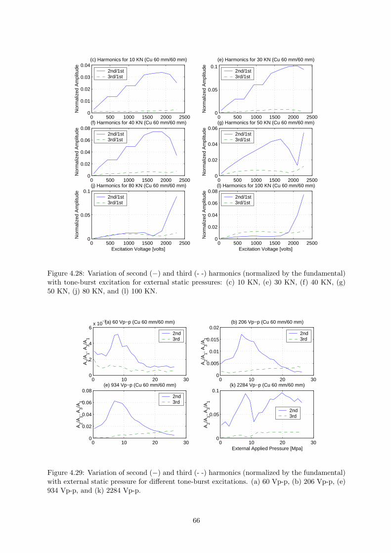
0 500 1000 1500 2000 25000

0.01

0.02

0.03

0.04

Nor

mal

ized

Am

plitu

de


2nd/1st3rd/1st

0 500 1000 1500 2000 25000

0.05

0.1

Nor

mal

ized

Am

plitu

de


2nd/1st3rd/1st

0 500 1000 1500 2000 25000

0.02

0.04

0.06

0.08

Nor

mal

ized

Am

plitu

de


2nd/1st3rd/1st

0 500 1000 1500 2000 25000

0.02

0.04

0.06

Nor

mal

ized

Am

plitu

de


2nd/1st3rd/1st

0 500 1000 1500 2000 25000

0.05

0.1


Nor

mal

ized

Am

plitu

de


2nd/1st3rd/1st

0 500 1000 1500 2000 25000

0.02

0.04

0.06

0.08


Nor

mal

ized

Am

plitu

de


2nd/1st3rd/1st

Figure 4.28: Variation of second (−) and third (- -) harmonics (normalized by the fundamental)with tone-burst excitation for external static pressures: (c) 10 KN, (e) 30 KN, (f) 40 KN, (g)50 KN, (j) 80 KN, and (l) 100 KN.

0 10 20 300

2

4

6x 10

−3(a) 60 Vp−p (Cu 60 mm/60 mm)

A2/A

1, A3/A

1

2nd3rd

0 10 20 300

0.005

0.01

0.015

0.02(b) 206 Vp−p (Cu 60 mm/60 mm)

A2/A

1, A3/A

1

2nd3rd

0 10 20 300

0.02

0.04

0.06

0.08(e) 934 Vp−p (Cu 60 mm/60 mm)

A2/A

1, A3/A

1

2nd3rd

0 10 20 300

0.05

0.1(k) 2284 Vp−p (Cu 60 mm/60 mm)


A2/A

1, A3/A

1

2nd3rd

Figure 4.29: Variation of second (−) and third (- -) harmonics (normalized by the fundamental)with external static pressure for different tone-burst excitations. (a) 60 Vp-p, (b) 206 Vp-p, (e)934 Vp-p, and (k) 2284 Vp-p.

66

4.4 Discussions and Conclusions

Ultrasonic nonlinearity of interfaces of two surfaces in contact have been investigated theoreti-cally and experimentally. A theory has been proposed that can be used to deal with ultrasonicnonlinearity of rough interfaces and smooth surfaces as well. It is the extension of Richardson’stheory for unbounded smooth interfaces. The calculations of ultrasonic interface nonlinearityhave been made for both smooth and rough interfaces. The results show that the smooth inter-face assumption yields overestimated nonlinearity than the rough interface assumption (mainlybased on the comparison of second harmonics). Since surfaces observed in nature are rough,the rough interface (consisting of two rough surfaces in contact) is a more accurate model forunbounded interfaces, kissing bonds in FSWs and joints, contact cracks in materials. For acontact rough interface, its ultrasonic response may have five different cases:

• (i) always in the completely closed state, and no nonlinearity occurs;

• (ii) varying alternately between the completely-closed state and the partially-closed;

• (iii) varying only in the partially-closed state, and no nonlinearity occurs;


• (v) varying alternately from the completely-closed state, to the partially-closed and thento the completely-open. In this case, the generation of interface nonlinearity might bemost efficient.

These cases have shown to be useful in the interpretation of the measurement results.

Experimental investigation of nonlinear ultrasonics of interfaces have been conducted basedon ultrasonic propagation technique. The measurements were made on four copper specimens(one without interface, and the others all with an interface) under different external staticpressure P0 and ultrasonic driving amplitudes E0. Observation of the measurement results haverevealed that

• large nonlinearity from contact interfaces are present under a modest static pressure P0

(e.g., 7 to 9 MPa).

• the static pressure P0 has a large impact on the nonlinear behavior of a contact interface.Under a modest P0 (e.g., 6 to 12 MPa), the interface shows strong nonlinear behavior,which is demonstrated by the presence of a strong second harmonic in the spectrum. Undera large P0, the interface nonlinearity becomes small because the interface is constrained inthe case of varying from the completely-closed state to the partially-closed. There seemsto exist a value of P0 on which the second harmonic (nonlinearity) becomes largest. Onthis value the ultrasonic response of the rough interface may mostly occur in the case (v)in which the interface varies alternately from the completely-closed state, to the partially-closed and then to the completely-open.

• the interface nonlinearity (from a contact interface) and the wave propagation nonlinearityresults in different asymmetries in waveforms: namely, the asymmetry due to interfacenonlinearity results in the spiky and prolonged negative part of waveforms, which coincideswith our theoretical prediction; the asymmetry because of the propagation nonlinearityleads to the round and shortened negative part.

The present research has shown that the propagation technique seems to work well to detectthe nonlinearity of contact interfaces. However, the kissing bonds usually have contact rough

67

interfaces with a small area. In this case, this propagation technique may not work so well. Ourprevious report [6] had shown that nonlinear behavior of small contacts in the copper specimens(bonded with hot isostatic pressing technique) could not be detected using this technique.

An extensive literature study of modulation techniques that has been conducted by us hasshown that nonlinear ultrasonic modulation technique can be more appropriate for detectingkissing bonds since the probing wave beam can be focused, and thus the local interaction ofultrasound with defects is easier to capture and detect.

In the future work, the first intention is to develop a nonlinear ultrasonic modulation tech-nique suitable for detecting kissing bonds and contact cracks with small local interfaces, andthe second is to extend the proposed theory (for contact interfaces) to treat kissing bonds, con-tact cracks and fatigue damages that are local interfaces and find more features on interfacenonlinearity to characterize the defects.

68

Bibliography

[1] The Welding Institute (TWI). Friction Stir Welding. http://www.twi.co.uk /j32k /unpro-tected/band 1/fswintro.html.

[2] Svensk Karnbranslehantering AB. FUD (Program for forskning, utveckling och demonstra-tion) 2001. EnaInfo Tryck, Enkoping, Sweden, 2001.

[3] Svensk Karnbranslehantering AB. Svensk Karnbranslehantering AB, Activities 2002.Tryckindustri Information AB, Solna, Sweden, 2003.

[4] The Welding Institute (TWI). Friction Stir Welding. http://www.twi.co.uk /j32k /unpro-tected/band 1/fswproc.html.

[5] A. Lammare and M. Moles. Ultrasound phased array inspection technology for the evalu-ation of friction stir welds. Proc. of the 15th World Conference on Nondestructive Testing,Roma, Italy. October 15-21 2000.

[6] T. Stepinski, F. Lingvall, E. Wennerstrom, and P. Wu. Inspection of copper canisters forspent nuclear fuel by means of ultrasound - nonlinear acoustics, synthetic aperture imaging.Technical Report TR-04-03, SKB, 2004.

[7] O. Buck, W. L. Morris, and J. M. Richardson. Acoustic harmonic generation at unbondedinterfaces and fatigue cracks. Appl. Phys. Lett., 33(5):371–373, September 1978.

[8] W. L. Morris, O. Buck, and R. V. Inman. Acoustic harmonic generation due to fatigedamage in high-srtength aluminum. J. Appl. Phys., 50(11):6737–6741, November 1979.

[9] L. Adler and P. B. Nagy. Second order nonlinearities and their applications in nde. Rev.Progr. QNDE, 10:1813–1820, 1991.

[10] P. B. Nagy. Excess nonlinearity in material containing microcracks. Rev. Progr. QNDE,13:1987–1994, 1994.

[11] P. B. Nagy. Fatigue damage assessment by nonlinear ultrasonic material characterization.Ultrasonics, 36:375–381, 1998.

[12] K.-Y. Jhang and K.-C. Kim. Evaluation of material degradation using nonlinear acousticeffect. Ultrasonics, 37:39–44, 1999.

[13] K.-Y. Jhang. Application of nonlinear ultrasonics to the nde of material degradation. IEEETrans. Ultrason. Ferroelectr.Freq. Contr., 47(3):540–548, 2000.

[14] H. Jeong, S.-H. Nahm, K.-Y. Jhang, and Y.-H. Nam. Nondestructive method for estimationof the fracture toughness of crmov rotor steels based on ultrasonic nonlinearity. Ultrasonics,41:543–549, 2003.

[15] I. Yu. Solodov, A. F. Asainov, and Ko sel Len. Non-linear saw reflection: experimentalevidence and nde apllications. Ultrasonics, 31(2):91–96, 1993.

[16] I. Yu. Solodov. Nonlinear nde using contact acoustic nonlinearity. 1994 IEEE UltrasonSymp., pages 1279–1283, 1994.

[17] I. Yu. Solodov. Ultrasonics of non-linear contacts: propagation, reflection and nde-applications. Ultrasonics, 36:383–390, 1998.

[18] I. Yu. Solodov, N. Krone, and G. Busse. Can: an example of nonlclassical acoustic nonlin-earity in solids. Ultrasonics, 40:621–625, 2002.

69

[19] C. J. Brotherhood, B. W. Drinkwater, and S. Dixon. The detectablity of kissing bonds inadhesive joints using ultrasonic techniques. Ultrasonics, 41:521–529, 2003.

[20] C. J. Brotherhood, B. W. Drinkwater, and F. J. Guild. The effect of compressive loadingon the ultrasonic detectability of kissing bonds in adhesive joints. J. of NDE, 21(3):95–104,2003.

[21] A. E. Ekimov, I. N. Didenkulov, and V. V. Kazakov. Modulation of torsional waves in arod with a crack. J. Acoust. Soc. Am., 106(3):1289–1292, 1999.

[22] D. Donskoy, A. Sutin, and A. Ekimov. Nonlinear acoustic interaction on contact interfacesand its use for nondestructive testing. NDT&E International, 34:231–238, 2001.

[23] Hui Xiao and P. Nagy. Enhanced ultrasonic detection of fatigue cracks by laser-inducedcrack closure. J. Appl. Phys., 83(12):7453–7460, 1998.

[24] Z. Yan and P. Nagy. Thermo-optical modulation for improved ultrasonic fatigue crackdetection in ti-6al-4v. NDT&E Interbnational, 33:213–223, 2000.

[25] Z. Yan and P. Nagy. Thermo-optical modulation of ultrasonic surface waves for nde. Ul-trasonics, 40:689–696, 2002.

[26] K. E-A. Van Den Abeele, P. A. Johnson, and A. Sutin. Nonlinear elastic wave spec-troscopy(news) techniques to discern material damage, part i: nonlinear wave modulationspectroscopy (nwms). Res. Nnodestr Eval, 12:17–30, 2000.

[27] K. E-A. Van Den Abeele, P. A. Johnson, and A. Sutin. Nonlinear elastic wave spec-troscopy(news) techniques to discern material damage, part ii: single-mode nonlinear res-onace acoustic spectroscopy (nwms). Res. Nnodestr Eval, 12:31–42, 2000.

[28] K. E-A. Van Den Abeele, A. Sutin, J. Carmeliet, and P. A. Johnson. Micro-damage di-agnostics using nonlinear elastic wave spectroscopy. NDT&E International, 34:239–248,2001.

[29] V. V. Kazakov, A. Sutin, and P. A. Johnson. Sensitive imaging of an elastic nonlinearwave-scattering source in a solid. Appl. Phys. Lett., 81(4):646–648, 2002.

[30] V. Yu. Zaitsev, P. Sas, and M. Wevers. Nonlinear modulation methods of structural damagedetection based on dissipative nonlinear effects. Proc. ISMA 25 Int. Conf. Noise VibrationEng, pages 233–242, Sept. 13-15 2000.

[31] V. Yu. Zaitsev, V. Gusev, and B. Castagnede. Observation of the ”luxemburg-gorky effect”for elastic waves. Ultrasonics, 40:627–631, 2002.

[32] V. Yu. Zaitsev, V. Gusev, and B. Castagnede. Luxemburg-gorky effect retooled for elasticwaves: a mechanism and experimental evidence. Phys. Rev. Lett., 89:105502–1–4, 2002.

[33] V. Zaitsev, V. Gusev, B. Castagnede, and P. Sas. Micro-damage detection using a mod-ulaion technique based on dissipative nonlinear effects. Forum Acusticum, Sevilla, Spain,September 16-20, 2002.

[34] J. M. Richardson. Harmonic generation at an unbonded interface – i. planar interfacebetween semi-infinite elastic media. Int. J. Engng. Sci., 17:73–85, 1979.

[35] J.-M. Baik and R. B. Thompson. Ultrasonic scattering from imperfect interfaces: a quasi-static model. J. Nondestr. Eval, 4:177–196, 1984.

70

[36] V. Gusev, B. Castagnede, and A. Moussatov. Hysteresis in response of nonlinear bistableinterface to continuously varying acoustic loading. Ultrasonics, 41(8):643–654, 2003.

[37] C. Pecorari. Nonlinear interaction of plane ultrasonic waves with an interface between roughsurfcaes in contact. J. Acoust. Soc. Am., 113(6):3065–3072, June 2003.

[38] K. L. Johnson. Contact mechanics. Cambrige University Press, New York, 1985.

[39] J. R. Barber and M. Ciavarella. Contact mechanics. Int. J. Solids Struct, 37:29–43, 2000.

[40] B. Bhshan. Micro/Nano Tribology. CRC Press, Boca Raton, 1999.

[41] S. R. Brown and C. H. Scholz. Closure of random elastic surfaces in contact. J. Goephys.Res, 90(B7):5531–5545, June 1985.

[42] J. A. Greenwood and J. B. P. Williamson. Contact of nominally flat surfaces. Proc. R. Soc.Lond. A, 295:300–319, 1966.

[43] A. Baltazar, S. I. Rokhlin, and C. Pecorari. On the relationship between ultrasonic andmicro-mechanical properties of contacting rough surfaces. J. Mech. Phys. Solids, 50:1397–1416, 2002.

71

4.A Theory on ultrasonic nonlinearity of contact interfaces

In this appendix a detailed derivation of the theory is given that describes the nonlinearityof an unbounded rough interface under ultrasonic plane wave disturbance. The interface underconsideration is planar and consists of two contacting rough surfaces of identical elastic materials.The theory is the extension of Richardson’s theory [34] that is only valid for the smooth interfacecase, and it can be used for both rough and smooth interfaces.

4.A.1 General Consideration

Since the problem of interest is concerned with the response of a rough interface to an ultrasonicplane wave, it can be formulated in terms of a one-dimensional wave motion. In this case theequation of motion in terms of particle displacement u = u(x, t) in an isotropic elastic mediumwith Lame constants λ and µ can be written as

ρ∂2u

∂t2=∂σ

∂x(4.14)

where ρ is the density, and σ = σ(x, t) is the stress. When an external hydrostatic compressivepressure P0 (that is uniform and nonnegative) is present in the medium, the stress-strain relationmay be assumed to be of the form

σ = (λ+ 2µ)ε− P0 = κ∂u

∂x− P0 (4.15)

where ε = ∂u/∂x is the strain, and κ = λ+2µ is the elastic constant. In Eq. (4.15), the referencestate of zero strain (and also zero displacement) is one of equilibrium with P0 (i.e., σ = −P0 forε=0) and with the interface closed at the origin. In convention, a stress is related to a strain inthe form σ = (λ+ 2µ)ε = κ∂u/∂x. In this case the reference state of zero strain corresponds tozero stress. In the present case the stress-strain relation in Eq. (4.15) is used because the stressis directly associated to the dynamic interfacial force due to ultrasonic disturbance.

Inserting σ in Eq. (4.15) into Eq. (4.14) leads to the wave equation

∂2u

∂t2= c2

∂2u

∂x2(4.16)

where c is the propagation speed of a longitudinal wave in an unbounded space, given by

c =√κ

ρ=

√λ+ 2µρ

(4.17)

Note that the static pressure P0 disappears in Eq. (4.16), which means that P0 does not influencethe dynamic process resulting from acoustic disturbance.

4.A.2 Characterization of rough surfaces and their contacts

An interface of two rough surfaces in contact manifests nonlinear mechanical behavior becausethe interface elasticity varies for compressive and tensile stresses. Such a contact rough in-terface is a good model for some defects in materials like kissing bonds in friction stir weldsand in adhesive joints. Such defects can be detected by exploiting their nonlinear responses toultrasound.

The ultrasonic response of a rough interface is determined by the surface properties (profilesand friction) of the two surfaces in contact. Assume that an unbounded rough interface is the

72

frictionless, elastic contact of two flat rough surfaces. The contact stresses depend only uponthe relative profile of the two surfaces, i.e., upon the shape of the gap between the surfacesbefore loading. A nominal flat rough surface contains a large number of asperities whose heightsvary randomly (Fig. 4.7). The heights of asperities are often characterized using Gaussiandistribution [41, 42] or inverted chi-square (χ2) distribution [41–43]. The inverted chi-squaredistribution is of the form

φ(z) =1

2n/2Γ(n/2)

(zmax − z

σ/√

2n

)(n−2)/2

exp(−zmax − z

2σ/√

2n

)(4.18)

where σ is the root-mean-square (rms) roughness, and zmax is the maximum height of asperities.Eq. (4.18) shows that the distribution requires two parameters to define its form: the standarddeviation σ and a parameter controlling its skewness, the number of degrees of freedom n. Theinverted chi-square distribution is simply a chi-square distribution with a variable substitutionsuch that it has a zero mean and is skewed toward positive heights. It is of the form

φ(z) =1

2n/2Γ(n/2)

(z

σ/√

2n

)(n−2)/2

exp(− z

2σ/√

2n

)(4.19)

which can be obtained by substituting zmax − z with z in Eq. (4.18).

The previous research [41] has shown that the inverted chi-distribution is better than Gaus-sian distribution because it fits the topography data better than the symmetric Gaussian dueto the skewness parameter n, and it becomes zero when the surface heights are larger than themaximum height, as does a real surface.

When two flat rough surfaces with rms roughnesses, σ1 and σ2, are pressed into contact soas to form a rough interface (Fig. 4.9 (a)), the interface can be converted into an equivalentinterface between a rigid smooth surface and a composite deformable rough surface (Fig. 4.9(b)). The distribution of the composite surface heights is still characterized by the invertedchi-square distribution,

φ(z) =1

2n/2Γ(n/2)

(z

σc/√

2n

)(n−2)/2

exp(− z

2σc/√

2n

)(4.20)

where σc is the composite surface rms roughness (σc =√σ2

1 + σ22). The effects of the surface

properties on the interfacial mechanics can be seen below.

4.A.3 Static responses of rough interfaces - Brown-Scholz’s model

When a rough interface is pressed by a hydrostatic pressure, the interface gap decreases (in otherwords, the relative approach increases). The relation between the external normal pressure Pand the relative approach δ (Fig. 4.10) between the two contacting surfaces can be determinedby Brown-Scholz’s model [43]

P (δ) =43Mψ

∫ δ

0(δ − z)3/2φ(z)dz (4.21)

where δ is the relative approach between the mean planes of the two rough surfaces, M =η〈E〉〈β1/2〉, η is the summit density of the composite surface, 〈E〉 is the average reduced elasticmodulus of contacting asperities, and 〈β1/2〉 is the average of the square root of the radius ofa composite peak, ψ is the factor due to the effect of misalignment. In the present case, it isassumed that ψ = 1.

73

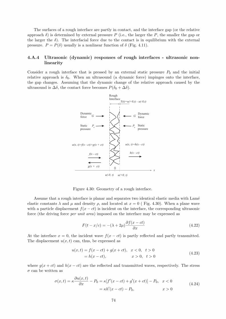
The surfaces of a rough interface are partly in contact, and the interface gap (or the relativeapproach δ) is determined by external pressure P (i.e., the larger the P , the smaller the gap orthe larger the δ). The interfacial force due to the contact is in equilibrium with the externalpressure. P = P (δ) usually is a nonlinear function of δ (Fig. 4.11).

4.A.4 Ultrasonic (dynamic) responses of rough interfaces - ultrasonic non-linearity

Consider a rough interface that is pressed by an external static pressure P0 and the initialrelative approach is δ0. When an ultrasound (a dynamic force) impinges onto the interface,the gap changes. Assuming that the dynamic change of the relative approach caused by theultrasound is ∆δ, the contact force becomes P (δ0 + ∆δ).

u(-0, t) u(+0, t)

x0

f(x - ct) h(x - ct)

u(x, t)=h(x - ct)

G

P0

P0

G

Y(t)=u(+0,t) - u(-0,t)

RoughInterface

Dynamicforce

Dynamicforce

Staticpressure

Staticpressure

u(x, t)=f(x - ct)+g(x + ct)

g(x + ct)

Figure 4.30: Geometry of a rough interface.

Assume that a rough interface is planar and separates two identical elastic media with Lameelastic constants λ and µ and density ρ, and located at x = 0 ( Fig. 4.30). When a plane wavewith a particle displacement f(x− ct) is incident on the interface, the corresponding ultrasonicforce (the driving force per unit area) imposed on the interface may be expressed as

F (t− x/c) = −(λ+ 2µ)∂f(x− ct)

∂x(4.22)

At the interface x = 0, the incident wave f(x − ct) is partly reflected and partly transmitted.The displacement u(x, t) can, thus, be expressed as

u(x, t) = f(x− ct) + g(x+ ct), x < 0, t > 0= h(x− ct), x > 0, t > 0

(4.23)

where g(x+ ct) and h(x− ct) are the reflected and transmitted waves, respectively. The stressσ can be written as

σ(x, t) = κ∂u(x, t)∂x

− P0 = κ[f ′(x− ct) + g′(x+ ct)] − P0, x < 0

= κh′(x− ct) − P0, x > 0(4.24)

74

At the interface the particle displacement becomes

u(+0, t) = f(−ct) + g(+ct), x < 0, t > 0u(−0, t) = h(−ct), x > 0, t > 0

(4.25)

the particle velocity is

u(+0, t) = −cf ′(−ct) + cg′(ct), x < 0, t > 0u(−0, t) = −ch′(−ct), x > 0, t > 0

(4.26)

and the stress is

σ(+0, t) = κ[f ′(−ct) + g′(+ct)] − P0, x < 0σ(−0, t) = κh′(−ct) − P0, x > 0

(4.27)

The relative motions of interface boundaries

Y (t) = u(+0, t) − u(−0, t) (4.28)

is defined as the interface opening displacement. The dynamic interfacial force (per unit area)on the contacting surfaces due to the ultrasonic displacement u(0, t) is defined as

G = −κ∂u(0, t)∂x

(4.29)

which is a function of Y .

When the interfacial gap is thin compared to the wavelength, the whole gap under ultrasonicdisturbance may be assumed to have the same dynamic behavior, and thus can be modelled by alumped system, which is a combination of distributed spring and mass [35]. This is the so-calledquasi-static approximation (QSA). According to the QSA, an interfacial imperfection causes adiscontinuity in the displacement that is proportional to the stress at the interface, while forinterfaces between the contacting surfaces, the components of the stress fields are assumed tobe continuous everywhere [43], namely,

σ(+0, t) = σ(−0, t) (4.30)

From the above condition and Eq. (4.27), it follows that

κ[f ′(−ct) + g′(+ct)] − P0 = κh′(−ct) − P0 (4.31)

which leads to the following relation (with consideration of the definition in Eq. (4.29))

G(Y ) = −κ[f ′(−ct) + g′(ct)]G(Y ) = −κh′(−ct)

(4.32)

From Eq. (4.26), and noting that Y (t) = u(+0, t)− u(−0, t) and c/κ = 1/(ρc) (since c2 = κ/ρ),Eq. (4.32) can be expressed as

ρcY (t) = 2G(Y ) − 2F (t) (4.33)

which is the equation that governs the motion of interface opening displacement Y (t) underultrasonic insonification. The solution of the equation provides us the (nonlinear) response ofthe interface to the ultrasound. Note that Y (t) ≥ 0 is always true, and G(Y ) is usually anonlinear function of Y (t).

For the initial relative approach δ0 due to the hydrostatic pressure P0, the initial interface gap(interface opening displacement) is assumed to be Y (0) = Y0. When the interface is disturbed

75

by an ultrasound, it may have three states (Fig. 4.13): completely closed (Y (t) = 0), partiallyclosed (0 < Y (t) ≤ Y0 + δ0), and completely open (Y (t) > Y0 + δ0).

When the interface gap is completely closed, we have

Y (t) = 0; Y (t) = 0 (4.34)

In this case, the interface vanishes, and Eq. (4.33) gives

G(Y ) = F (t) (4.35)

When the interface is completely open (Y (t) > Y0 + δ0), the stress on the interface surfacesvanish, and then we have

σ(±0, t) = −G(Y ) − P0 = 0 (4.36)

which leads toG(Y ) = −P0 (4.37)

In this case, Eq. (4.33) becomes

ρcY (t) = −2P0 − 2F (t) (4.38)

When the interface is partially closed (0 < Y (t) ≤ Y0 + δ0), Eq. (4.33) can be solved if G(Y ) isknown. If G(Y ) is a linear function of Y , then Eq. (4.33) may have analytical solution. However,G(Y ) in practice is mostly a nonlinear function of Y , thus one has to resort to numerical solution.

For a smooth interface, the gap only has two states: closed and open. It is just a special caseof a rough interface without partially-closed state. Thus, Eq. (4.33) also applies to the smoothinterface.

After Y (t) and u(±0, t) are determined, and from Y (t) = u(+0, t)− u(−0, t) and Eq. (4.25),the reflected wave g(x+ ct) and the transmitted wave h(x− ct) can be found as follows

g(x+ ct) = −12Y(t+

x

c

)(4.39)

andh(x− ct) = f(x− ct) +

12Y(t− x

c

)(4.40)

The above two relations are useful because reflection or transmission is usually detected by areceiving transducer.

A. Ultrasonic nonlinearity of an unbounded smooth interface

Consider an incident wave of a sinusoid

f(x− ct) = −A sin(kx− ωt) (4.41)

which at the interface x = 0 becomes

f(0 − ct) = A sin(ωt) (4.42)

The driving force on the interface is (Eq. (4.22))

F (t) = −κ∂f(x− ct)∂x

|x=0 = κkA cos(−ωt) = ρcωA cos(−ωt) = B cos(ωt) (4.43)

whereB = ρcωA (4.44)

76

A smooth interface may only have two states: closed (Y (t) = 0) and open (Y (t) > 0). For aclosed interface, the interface opening displacement is

Y (t) = 0 (4.45)

and the interfacial force isG(Y ) = F (t) (4.46)

When the interface is open, one has G(Y ) = −P0 (Eq. (4.37)), and the governing equation ofinterface opening displacement (Eq. (4.38)) becomes

ρcY (t) = −2P0 − 2B cos(ωt) (4.47)

The solution to the above differential equation is

Y (t) = − 2ρc

∫[P0 +B cos(ωt)]dt = − 2

ρc

[P0t+

B

ωsin(ωt)

]+ C

= −2A [ηωt+ sin(ωt)] + C

(4.48)

whereη = P0/B (4.49)

and C is the arbitrary constant that can be determined from the ”initial” conditions at t = ti,

C(ti) = Y (ti) + 2A [ηωti + sin(ωti)] (4.50)

C(ti) needs to be calculated when the gap changes from the closed state to the open state,because Eq. (4.48) is valid only for the open gap. The relation of G(Y ) with Y is nonlinearprovided that |F (t)| > P0 (see Fig. 4.4).

B. Ultrasonic nonlinearity of unbounded rough interfaces

An unbounded rough interface under ultrasonic disturbance may have three states (Fig. 4.13):completely closed (Y (t) = 0), partially closed (0 < Y (t) ≤ Y0 + δ0), and completely open(Y (t) > Y0 + δ0). The partially-closed state of a rough interface is the only difference from asmooth surface. The solution of Eq (4.33) for the closed and open states in the rough interfacecase are similar to those in the smooth interface case.

A rough interface in reality has a nonlinear stiffness (i.e., G(Y ) nonlinearly depends on Yin the partially closed state, 0 < Y (t) ≤ Y0 + δ0) [41, 43]. Here, however, we consider arough interface with a linear stiffness, which can be seen as a simplified case of some real roughinterfaces. For such an interface, an analytical solution to Eq (4.33) is available. For the solutionto a rough interface with a nonlinear stiffness one can resort to numerical calculation.

Assume that the rough interface has a linear interfacial stiffness for 0 < Y (t) < Y (0) + δ0

G(Y ) = −κ0[Y (t) − Y0] (4.51)

where Y0 is the initial equilibrium thickness of the interface, and κ0 is the normal interfacialstiffness constant.

When the interface is completely closed, then

Y (t) = 0; G(Y ) = F (t) (4.52)

When the interface is completely open (Y (t) > Y0 + δ0), Y (t) can be determined in the sameway as in the smooth interface case

Y (t) = −2A [ηωt+ sin(ωt)] + Co (4.53)

77

where the arbitrary constant Co can be found from the ”initial” conditions at t = ti,

Co(ti) = Y (ti) + 2A [ηωti + sin(ωti)] (4.54)

Note that Co(ti) needs to be calculated when the gap changes from the partially-closed state tothe open state. The interfacial force for the open gap is

G(Y ) = −κ0δ0 = −P0 (4.55)

For the partially-closed interface (0 < Y (t) < Y0 + δ0), inserting Eq. (4.51) into Eq. (4.33) yields

ρc ˙Y (t) = −κ0[Y (t) − Y0] − 2F (t) (4.56)

Since the solution to equation y+P (t)y = Q(t) is y(t) = e−∫P (t)dt

[∫Q(t)eintP (t)dtdt+ C

], and

considering F (t) = ρcωA cos(ωt), the solution to Eq. (4.56) can be found to be

Y (t) − Y0 = exp(−ξt){−2ωA

exp(ξt)ξ2 + ω2

[ξ cos(ωt) + ω sin(ωt)] + Cp

}(4.57)

whereξ =

2κ0

ρc(4.58)

and Cp is determined by the initial value of Y (tj) at t = tj ,

Cp(tj) = exp(ξtj){

[Y (tj) − Y0] +2ωA

ξ2 + ω2[ξ cos(ωtj) + ω sin(ωtj)]

}(4.59)

Cp(tj) should be calculated when the interface gap changes either from the open state to thepartially-closed state or from the completely-closed state to the partially-closed state if the statesare present. For the initial condition Y (0) = Y0 at t = 0, one may have

Cp(0) =2ωξAξ2 + ω2

(4.60)

The interface opening displacement in this case becomes

Y (t) =−2ωAξ2 + ω2

[ξ cos(ωt) + ω sin(ωt)] + exp(−ξt) 2ωξAξ2 + ω2

+ Y0 (4.61)

and the interfacial force is

G(Y ) = −κ0

{−2ωAξ2 + ω2

[ξ cos(ωt) + ω sin(ωt)] + exp(−ξt) 2ωξAξ2 + ω2

}(4.62)

For a rough interface with nonlinear interfacial stiffness as shown in Fig. 4.13, one can resortto the numerical computation. If an appropriate polynomial is applied to fit the nonlinearrelation between G(Y ) and Y , the differential equation (Eq. (4.33)) can be comparatively easyto solve.

78

4.B Measurement results

79

0 10 20 30 40 50−2

−1

0

1

2

Time t [µs]

Sig

nal a

mpl

itude

[vol

ts]


0 1 2 3 4 510

−6

10−4

10−2

100


0 10 20 30 40 50−6

−4

−2

0

2

4

6

Time t [µs]

Sig

nal a

mpl

itude

[vol

ts]


0 1 2 3 4 510

−6

10−4

10−2

100


0 10 20 30 40 50−15

−10

−5

0

5

10

15

Time t [µs]S

igna

l am

plitu

de [v

olts

]

(c) 30 KN (90 mm/00 mm) for 431 v−pp excitation

0 1 2 3 4 510

−6

10−4

10−2

100

(c´) Spectrum of the signal in (c)

0 10 20 30 40 50

−20

−10

0

10

20

Time t [µs]

Sig

nal a

mpl

itude

[vol

ts]


0 1 2 3 4 510

−6

10−4

10−2

100


0 10 20 30 40 50

−30

−20

−10

0

10

20

30

Time t [µs]

Sig

nal a

mpl

itude

[vol

ts]

(g) 30 KN (90 mm/00 mm) for 1408 v−pp excitation

0 1 2 3 4 510

−6

10−4

10−2

100

(g´) Spectrum of the signal in (g)

0 10 20 30 40 50−40

−20

0

20

40

Time t [µs]

Sig

nal a

mpl

itude

[vol

ts]

(h) 30 KN (90 mm/00 mm) for 1653 v−pp excitation

0 1 2 3 4 510

−6

10−4

10−2

100

(h´) Spectrum of the signal in (h)

0 10 20 30 40 50−40

−20

0

20

40

Time t [µs]

Sig

nal a

mpl

itude

[vol

ts]

(i) 30 KN (90 mm/00 mm) for 1888 v−pp excitation

0 1 2 3 4 510

−6

10−4

10−2

100

(i´) Spectrum of the signal in (i)

0 10 20 30 40 50−40

−20

0

20

40

Time t [µs]

Sig

nal a

mpl

itude

[vol

ts]

(j) 30 KN (90 mm/00 mm) for 2101 v−pp excitation

0 1 2 3 4 510

−6

10−4

10−2

100

(j´) Spectrum of the signal in (j)

0 10 20 30 40 50−40

−20

0

20

40

Time t [µs]

Sig

nal a

mpl

itude

[vol

ts]


0 1 2 3 4 510

−6

10−4

10−2

100


Figure 4.31: Measurements on Specimen CUCYL 0 for different tone-burst excitations E0 andfixed external force P0=30 KN. (a) to (k) Waveforms, and (a) to (k) their spectra.

80

0 10 20 30 40 50−2

−1

0

1

2

Time t [µs]

Sig

nal a

mpl

itude

[vol

ts]


0 1 2 3 4 510

−6

10−4

10−2

100


0 10 20 30 40 50−8

−6

−4

−2

0

2

4

6

8

Time t [µs]

Sig

nal a

mpl

itude

[vol

ts]


0 1 2 3 4 510

−6

10−4

10−2

100


0 10 20 30 40 50−15

−10

−5

0

5

10

15

Time t [µs]

Sig

nal a

mpl

itude

[vol

ts]

(c) 100 KN (90 mm/00 mm) for 431 v−pp excitation

0 1 2 3 4 510

−6

10−4

10−2

100


0 10 20 30 40 50−20

−10

0

10

20

Time t [µs]S

igna

l am

plitu

de [v

olts

]

(d) 100 KN (90 mm/00 mm) for 675 v−pp excitation

0 1 2 3 4 510

−6

10−4

10−2

100

(d´) Spectrum of the signal in (d)

0 10 20 30 40 50

−20

−10

0

10

20

Time t [µs]

Sig

nal a

mpl

itude

[vol

ts]


0 1 2 3 4 510

−6

10−4

10−2

100


0 10 20 30 40 50

−30

−20

−10

0

10

20

30

Time t [µs]

Sig

nal a

mpl

itude

[vol

ts]

(f) 100 KN (90 mm/00 mm) for 1179 v−pp excitation

0 1 2 3 4 510

−6

10−4

10−2

100

(f´) Spectrum of the signal in (f)

0 10 20 30 40 50

−30

−20

−10

0

10

20

30

Time t [µs]

Sig

nal a

mpl

itude

[vol

ts]

(g) 100 KN (90 mm/00 mm) for 1408 v−pp excitation

0 1 2 3 4 510

−6

10−4

10−2

100


0 10 20 30 40 50−40

−20

0

20

40

Time t [µs]

Sig

nal a

mpl

itude

[vol

ts]

(h) 100 KN (90 mm/00 mm) for 1653 v−pp excitation

0 1 2 3 4 510

−6

10−4

10−2

100


0 10 20 30 40 50

−40

−20

0

20

40

Time t [µs]

Sig

nal a

mpl

itude

[vol

ts]

(i) 100 KN (90 mm/00 mm) for 1888 v−pp excitation

0 1 2 3 4 510

−6

10−4

10−2

100


0 10 20 30 40 50

−40

−20

0

20

40

Time t [µs]

Sig

nal a

mpl

itude

[vol

ts]

(j) 100 KN (90 mm/00 mm) for 2101 v−pp excitation

0 1 2 3 4 510

−6

10−4

10−2

100


0 10 20 30 40 50

−40

−20

0

20

40

Time t [µs]

Sig

nal a

mpl

itude

[vol

ts]


0 1 2 3 4 510

−6

10−4

10−2

100



81

20 30 40 50

−1

−0.5

0

0.5

1

Time t [µs]

Sig

nal a

mpl

itude

[vol

ts]


0 1 2 3 4 510

−6

10−4

10−2

100

Frequency f [MHz]


20 30 40 50−4

−2

0

2

4

Time t [µs]

Sig

nal a

mpl

itude

[vol

ts]


0 1 2 3 4 510

−6

10−4

10−2

100

Frequency f [MHz]


20 30 40 50−8

−6

−4

−2

0

2

4

6

8

Time t [µs]

Sig

nal a

mpl

itude

[vol

ts]

(c) Cylind 3 (60 mm/60 mm) for 30 KN & 431 Vp−p

0 1 2 3 4 510

−6

10−4

10−2

100

Frequency f [MHz]


20 30 40 50

−10

−5

0

5

10

Time t [µs]

Sig

nal a

mpl

itude

[vol

ts]

(d) Cylind 3 (60 mm/60 mm) for 30 KN & 675 Vp−p

0 1 2 3 4 510

−6

10−4

10−2

100

Frequency f [MHz]


20 30 40 50−15

−10

−5

0

5

10

15

Time t [µs]

Sig

nal a

mpl

itude

[vol

ts]


0 1 2 3 4 510

−6

10−4

10−2

100

Frequency f [MHz]


20 30 40 50−20

−10

0

10

20

Time t [µs]

Sig

nal a

mpl

itude

[vol

ts]

(f) Cylind 3 (60 mm/60 mm) for 30 KN & 1179 Vp−p

0 1 2 3 4 510

−6

10−4

10−2

100

Frequency f [MHz]


20 30 40 50−20

−10

0

10

20

Time t [µs]

Sig

nal a

mpl

itude

[vol

ts]

(g) Cylind 3 (60 mm/60 mm) for 30 KN & 1408 Vp−p

0 1 2 3 4 510

−6

10−4

10−2

100

Frequency f [MHz]


20 30 40 50

−20

−10

0

10

20

Time t [µs]

Sig

nal a

mpl

itude

[vol

ts]

(h) Cylind 3 (60 mm/60 mm) for 30 KN & 1653 Vp−p

0 1 2 3 4 510

−6

10−4

10−2

100

Frequency f [MHz]


20 30 40 50

−20

−10

0

10

20

Time t [µs]

Sig

nal a

mpl

itude

[vol

ts]

(i) Cylind 3 (60 mm/60 mm) for 30 KN & 1888 Vp−p

0 1 2 3 4 510

−6

10−4

10−2

100

Frequency f [MHz]


20 30 40 50

−20

−10

0

10

20

Time t [µs]

Sig

nal a

mpl

itude

[vol

ts]

(j) Cylind 3 (60 mm/60 mm) for 30 KN & 2101 Vp−p

0 1 2 3 4 510

−6

10−4

10−2

100

Frequency f [MHz]


20 30 40 50

−20

−10

0

10

20

Time t [µs]

Sig

nal a

mpl

itude

[vol

ts]


0 1 2 3 4 510

−6

10−4

10−2

100

Frequency f [MHz]



82

20 30 40 50−1.5

−1

−0.5

0

0.5

1

1.5

Time t [µs]

Sig

nal a

mpl

itude

[vol

ts]


0 1 2 3 4 510

−6

10−4

10−2

100

Frequency f [MHz]


20 30 40 50−5

0

5

Time t [µs]

Sig

nal a

mpl

itude

[vol

ts]


0 1 2 3 4 510

−6

10−4

10−2

100

Frequency f [MHz]


20 30 40 50−10

−5

0

5

10

Time t [µs]

Sig

nal a

mpl

itude

[vol

ts]

(c) Cylind 3 (60 mm/60 mm) for 100 KN & 431 Vp−p

0 1 2 3 4 510

−6

10−4

10−2

100

Frequency f [MHz]


20 30 40 50−15

−10

−5

0

5

10

15

Time t [µs]

Sig

nal a

mpl

itude

[vol

ts]

(d) Cylind 3 (60 mm/60 mm) for 100 KN & 675 Vp−p

0 1 2 3 4 510

−6

10−4

10−2

100

Frequency f [MHz]


20 30 40 50−20

−10

0

10

20

Time t [µs]

Sig

nal a

mpl

itude

[vol

ts]


0 1 2 3 4 510

−6

10−4

10−2

100

Frequency f [MHz]


20 30 40 50

−20

−10

0

10

20

Time t [µs]

Sig

nal a

mpl

itude

[vol

ts]

(f) Cylind 3 (60 mm/60 mm) for 100 KN & 1179 Vp−p

0 1 2 3 4 510

−6

10−4

10−2

100

Frequency f [MHz]


20 30 40 50−30

−20

−10

0

10

20

30

Time t [µs]

Sig

nal a

mpl

itude

[vol

ts]

(g) Cylind 3 (60 mm/60 mm) for 100 KN & 1408 Vp−p

0 1 2 3 4 510

−6

10−4

10−2

100

Frequency f [MHz]


20 30 40 50−30

−20

−10

0

10

20

30

Time t [µs]

Sig

nal a

mpl

itude

[vol

ts]

(h) Cylind 3 (60 mm/60 mm) for 100 KN & 1653 Vp−p

0 1 2 3 4 510

−6

10−4

10−2

100

Frequency f [MHz]


20 30 40 50

−30

−20

−10

0

10

20

30

Time t [µs]

Sig

nal a

mpl

itude

[vol

ts]

(i) Cylind 3 (60 mm/60 mm) for 100 KN & 1888 Vp−p

0 1 2 3 4 510

−6

10−4

10−2

100

Frequency f [MHz]


20 30 40 50

−30

−20

−10

0

10

20

30

Time t [µs]

Sig

nal a

mpl

itude

[vol

ts]

(j) Cylind 3 (60 mm/60 mm) for 100 KN & 2101 Vp−p

0 1 2 3 4 510

−6

10−4

10−2

100

Frequency f [MHz]


20 30 40 50

−30

−20

−10

0

10

20

30

Time t [µs]

Sig

nal a

mpl

itude

[vol

ts]


0 1 2 3 4 510

−6

10−4

10−2

100

Frequency f [MHz]



83

0 500 1000 1500 2000 25000

0.005

0.01

0.015

Nor

mal

ized

Am

plitu

de

(a) Harmonics for 0 KN (Cu 90 mm/00 mm)

2nd/1st3rd/1st

0 500 1000 1500 2000 25000

0.01

0.02

0.03

0.04

Nor

mal

ized

Am

plitu

de


2nd/1st3rd/1st

0 500 1000 1500 2000 25000

0.01

0.02

0.03

Nor

mal

ized

Am

plitu

de

(d) Harmonics for 20 KN (Cu 90 mm/00 mm)

2nd/1st3rd/1st

0 500 1000 1500 2000 25000

0.05

0.1


Nor

mal

ized

Am

plitu

de


2nd/1st3rd/1st

0 500 1000 1500 2000 25000

0.05

0.1

0.15

0.2


Nor

mal

ized

Am

plitu

de


2nd/1st3rd/1st

0 500 1000 1500 2000 25000

0.05

0.1

0.15

0.2

Nor

mal

ized

Am

plitu

de


2nd/1st3rd/1st

0 500 1000 1500 2000 25000

0.05

0.1

0.15

0.2

Nor

mal

ized

Am

plitu

de

(h) Harmonics for 60 KN (Cu 90 mm/00 mm)

2nd/1st3rd/1st

0 500 1000 1500 2000 25000

0.05

0.1

0.15

0.2

Nor

mal

ized

Am

plitu

de

(i) Harmonics for 70 KN (Cu 90 mm/00 mm)

2nd/1st3rd/1st

0 500 1000 1500 2000 25000

0.05

0.1

0.15

0.2

Nor

mal

ized

Am

plitu

de


2nd/1st3rd/1st

0 500 1000 1500 2000 25000

0.05

0.1

0.15

0.2


Nor

mal

ized

Am

plitu

de

(k) Harmonics for 90 KN (Cu 90 mm/00 mm)

2nd/1st3rd/1st

0 500 1000 1500 2000 25000

0.05

0.1

0.15

0.2


Nor

mal

ized

Am

plitu

de


2nd/1st3rd/1st

Figure 4.35: Variation of second (−) and third (- -) harmonics (normalized by the fundamental)with tone-burst excitation for external static pressures: (a) 1 KN, (c) 10 KN, (d) 20 KN, (e) 30KN, (f) 40 KN, (g) 50 KN, (h) 60 KN, (i) 70 KN, (j) 80 KN, (k) 90 KN, (l) 100 KN.

84

0 10 20 300

1

2

3x 10

−3(a) 60 Vp−p (Cu 90 mm/00 mm)

A2/A

1, A3/A

1

2nd3rd

0 10 20 301.5

2

2.5

3

3.5x 10

−3(b) 206 Vp−p (Cu 90 mm/00 mm)

A2/A

1, A3/A

1

2nd3rd

0 10 20 300

2

4

6

8x 10

−3(c) 431 Vp−p (Cu 90 mm/00 mm)

A2/A

1, A3/A

1

2nd3rd

0 10 20 300

0.005

0.01(d) 675 Vp−p (Cu 90 mm/00 mm)

A2/A

1, A3/A

1

2nd3rd

0 10 20 300

0.005

0.01

0.015(e) 934 Vp−p (Cu 90 mm/00 mm)

A2/A

1, A3/A

1

2nd3rd

0 10 20 300

0.005

0.01

0.015(f) 1179 Vp−p (Cu 90 mm/00 mm)

A2/A

1, A3/A

1

2nd3rd

0 10 20 300.005

0.01

0.015

0.02

0.025(g) 1408 Vp−p (Cu 90 mm/00 mm)

A2/A

1, A3/A

1

2nd3rd

0 10 20 300

0.01

0.02

0.03(h) 1653 Vp−p (Cu 90 mm/00 mm)

A2/A

1, A3/A

1

2nd3rd

0 10 20 300

0.02

0.04

0.06(i) 1888 Vp−p (Cu 90 mm/00 mm)

A2/A

1, A3/A

1

2nd3rd

0 10 20 300

0.05

0.1

0.15

0.2(j) 2101 Vp−p (Cu 90 mm/00 mm)


A2/A

1, A3/A

1

2nd3rd

0 10 20 300

0.05

0.1

0.15

0.2(k) 2284 Vp−p (Cu 90 mm/00 mm)


A2/A

1, A3/A

1

2nd3rd

Figure 4.36: Variation of second (−) and third (- -) harmonics (normalized by the fundamental)with external static pressure for different tone-burst excitations. (a) 60 Vp-p, (b) 206 Vp-p, (c)431 Vp-p, (d) 675 Vp-p, (e) 934 Vp-p, (f) 1179 Vp-p, (g) 1408 Vp-p, (h) 1653 Vp-p, (i) 1888Vp-p, (j) 2101 Vp-p, and (k) 2284 Vp-p.

85

0 500 1000 1500 2000 25000

0.01

0.02

0.03

Nor

mal

ized

Am

plitu

de

(a) Harmonics for 1 KN (Cu 60 mm/60 mm)

2nd/1st3rd/1st

0 500 1000 1500 2000 25000

0.01

0.02

0.03

0.04

Nor

mal

ized

Am

plitu

de


2nd/1st3rd/1st

0 500 1000 1500 2000 25000

0.02

0.04

0.06

0.08

Nor

mal

ized

Am

plitu

de

(d) Harmonics for 20 KN (Cu 60 mm/60 mm)

2nd/1st3rd/1st

0 500 1000 1500 2000 25000

0.05

0.1

Nor

mal

ized

Am

plitu

de


2nd/1st3rd/1st

0 500 1000 1500 2000 25000

0.02

0.04

0.06

0.08


Nor

mal

ized

Am

plitu

de


2nd/1st3rd/1st

0 500 1000 1500 2000 25000

0.02

0.04

0.06


Nor

mal

ized

Am

plitu

de


2nd/1st3rd/1st

0 500 1000 1500 2000 25000

0.05

0.1

Nor

mal

ized

Am

plitu

de

(h) Harmonics for 60 KN (Cu 60 mm/60 mm)

2nd/1st3rd/1st

0 500 1000 1500 2000 25000

0.05

0.1

Nor

mal

ized

Am

plitu

de

(i) Harmonics for 70 KN (Cu 60 mm/60 mm)

2nd/1st3rd/1st

0 500 1000 1500 2000 25000

0.05

0.1

Nor

mal

ized

Am

plitu

de


2nd/1st3rd/1st

0 500 1000 1500 2000 25000

0.02

0.04

0.06

0.08


Nor

mal

ized

Am

plitu

de

(k) Harmonics for 90 KN (Cu 60 mm/60 mm)

2nd/1st3rd/1st

0 500 1000 1500 2000 25000

0.02

0.04

0.06

0.08


Nor

mal

ized

Am

plitu

de


2nd/1st3rd/1st

Figure 4.37: Variation of second (−) and third (- -) harmonics (normalized by the fundamental)with tone-burst excitation for external static pressures: (a) 1 KN, (c) 10 KN, (d) 20 KN, (e) 30KN, (f) 40 KN, (g) 50 KN, (h) 60 KN, (i) 70 KN, (j) 80 KN, (k) 90 KN, (l) 100 KN.

86

0 10 20 300

2

4

6x 10

−3(a) 60 Vp−p (Cu 60 mm/60 mm)

A2/A

1, A3/A

1

2nd3rd

0 10 20 300

0.005

0.01

0.015

0.02(b) 206 Vp−p (Cu 60 mm/60 mm)

A2/A

1, A3/A

1

2nd3rd

0 10 20 300

0.01

0.02

0.03

0.04(c) 431 Vp−p (Cu 60 mm/60 mm)

A2/A

1, A3/A

1

2nd3rd

0 10 20 300

0.01

0.02

0.03

0.04(d) 675 Vp−p (Cu 60 mm/60 mm)

A2/A

1, A3/A

1

2nd3rd

0 10 20 300

0.02

0.04

0.06

0.08(e) 934 Vp−p (Cu 60 mm/60 mm)

A2/A

1, A3/A

1

2nd3rd

0 10 20 300

0.02

0.04

0.06

0.08(f) 1179 Vp−p (Cu 60 mm/60 mm)

A2/A

1, A3/A

1

2nd3rd

0 10 20 300

0.05

0.1(g) 1408 Vp−p (Cu 60 mm/60 mm)

A2/A

1, A3/A

1

2nd3rd

0 10 20 300

0.05

0.1(h) 1653 Vp−p (Cu 60 mm/60 mm)

A2/A

1, A3/A

1

2nd3rd

0 10 20 300

0.05

0.1(i) 1888 Vp−p (Cu 60 mm/60 mm)

A2/A

1, A3/A

1

2nd3rd

0 10 20 300

0.05

0.1(j) 2101 Vp−p (Cu 60 mm/60 mm)


A2/A

1, A3/A

1

2nd3rd

0 10 20 300

0.05

0.1(k) 2284 Vp−p (Cu 60 mm/60 mm)


A2/A

1, A3/A

1

2nd3rd

Figure 4.38: Variation of second (−) and third (- -) harmonics (normalized by the fundamental)with external static pressure for different tone-burst excitations. (a) 60 Vp-p, (b) 206 Vp-p, (c)431 Vp-p, (d) 675 Vp-p, (e) 934 Vp-p, (f) 1179 Vp-p, (g) 1408 Vp-p, (h) 1653 Vp-p, (i) 1888Vp-p, (j) 2101 Vp-p, and (k) 2284 Vp-p.

87

tr-04-24 - skb

Documents