SINTEF Energy Research

Energy Systems

2012-01-13

TR A7184- Unrestricted

Report

Evaluation of radar-derived precipitation

estimates using runoff simulation

Report for the NFR Energy Norway funded project "Utilisation of weather radar data in

atmospheric and hydrological models"

Author(s)

Yisak Sultan Abdella

Kolbjørn Engeland

Jean-Marie Lepioufle

PROJECT NO. 12X649.

REPORT NO. TR A7184

VERSION 1

2 of 20

Document history

VERSION DATE VERSION DESCRIPTION

1. 2012-01-13 Final version

PROJECT NO. 12X649.

REPORT NO. TR A7184

VERSION 1

3 of 20

Table of contents

1 Introduction .................................................................................................................................................................................................................... 4

2 Study regions ................................................................................................................................................................................................................ 4

3 Precipitation input ..................................................................................................................................................................................................... 7

3.1 Interpolated precipitation ..............................................................................................................................................................................7

3.2 Radar-derived precipitation .........................................................................................................................................................................8

3.3 Combined precipitation ....................................................................................................................................................................................8

3.4 Spatially aggregated precipitation ..........................................................................................................................................................8

4 Evaluation catchments ........................................................................................................................................................................................... 8

5 Hydrologic models .................................................................................................................................................................................................. 12

5.1 ENKI Distributed model ................................................................................................................................................................................ 12

5.2 Standard HBV model ...................................................................................................................................................................................... 12

6 Evaluation procedure ........................................................................................................................................................................................... 12

6.1 Distributed model set-up ............................................................................................................................................................................ 13

6.2 Lumped model set-up .................................................................................................................................................................................... 13

7 Results ............................................................................................................................................................................................................................ 13

7.1 RISSA-region ........................................................................................................................................................................................................ 13

7.1.1 Distributed model runs .............................................................................................................................................................. 13

7.1.2 Lumped model runs ...................................................................................................................................................................... 16

7.2 HGB-region ............................................................................................................................................................................................................ 18

8 Conclusions ................................................................................................................................................................................................................. 19

9 References ................................................................................................................................................................................................................... 20

PROJECT NO. 12X649.

REPORT NO. TR A7184

VERSION 1

4 of 20

1 Introduction

This report presents the results from sub project 3.2 in the project called " Utilisation of weather radar data in atmospheric and hydrological models" funded by the Norwegian Research Council and Energy Norway. The subproject has been executed by Sintef Energy Research and the participating power companies. Current hydrologic modelling within the power sector usually involves hourly or daily precipitation data obtained from a network of rain gauges. The spatial distribution of precipitation inferred by interpolation from point observations in gages introduces errors due to the imprecise knowledge of precipitation distribution in space and requires a dense network of gauges, which is available only for a few catchments. In recent years, however, the implementation of weather radars in Norway by the Norwegian Meteorological Institute (met.no) has made radar a potential tool to improve estimation of precipitation between the gauges. Weather radars offer an advantage over rain gauges in that they can provide high resolution data with a spatial scale of the order of 1km and a temporal scale of down to 5 minutes. They cover extended areas, with a spatial extent of up to several hundred kilometers, from one single measurement site. These characteristics make weather radars well suited to hydrological applications. However, quantitative precipitation is not directly measured by weather radars but is derived from measurements of radar reflectivity. Both the reflectivity measurements themselves and the process of converting them to precipitation rates are subject to errors and uncertainties. Therefore, radar precipitation estimates have to be corrected before their use in hydrology. But previous studies have shown that there would be a bias remaining in such purely radar-based precipitation estimates even after correction. In order to remove or minimize this bias and obtain more accurate estimates, precipitation derived from radar measurements is often combined with rain gauge observations or data derived from them. These two data sources are generally considered as complementary and assumed as independent estimates of the same unknown quantity. In view of the above, the objective of sub project 3.2 is to evaluate both rain gauge- and radar-based precipitation inputs using hydrologic models. Two regions in central and southern Norway were selected for the project. The following three precipitation products were generated and evaluated: (1) precipitation interpolated from rain gauges, (2) precipitation derived from radar measurements and (3) a combination of the first two products. Both Sintef Energy and the participation power companies ran their models using the generated inputs. Sintef Energi used a distributed hydrologic model while the power companies used their lumped operational HBV model. The report is organized as follows: Section 2 presents the study regions. The different precipitation inputs are described in section 3. Section 4 shows the selected catchments within the study regions and section 5 presents the models used. The evaluation procedure is given in section 6. Section 7 shows the results of the evaluation upon which conclusions are drawn in section 8.

2 Study regions

Two study regions have been selected for this project (Fig.1). The first region (referred to as RISSA-region in this report) is located within the scanning coverage of the Rissa radar and has an areal extent of 221x210km. The second region (referred to as HGB-region in this report) is located within the scanning coverage of the Hægebostad radar and has an areal extent of 202x212km. Since the catchments operated by the participating power companies are situated in central and southern Norway, only the five radars within these parts of the country were considered for the study. The Rissa and Hægebostad radars were selected from the five radars because they are the ones with the least amount of blockage and the highest number of catchments within their scanning range. Figures 2 - 6 show the beam blockage for the radars in central and southern Norway. The figures also show precipitation accumulation over 22 months for all the radars except Stadt where 14 months are available. Accumulation for Hurum is not yet available and is therefore not shown here.

PROJECT NO. 12X649.

REPORT NO. TR A7184

VERSION 1

5 of 20

Figure 1Study regions

Figure 2 Calculated beam blockage for Hurum radar

PROJECT NO. 12X649.

REPORT NO. TR A7184

VERSION 1

6 of 20

Figure 3 a) Calculated beam blockage and b) accumulated precipitation for Hægebostad radar

Figure 4 a) Calculated beam blockage and b) accumulated precipitation for Bømlo radar

a b

PROJECT NO. 12X649.

REPORT NO. TR A7184

VERSION 1

7 of 20

Figure 5 a) Calculated beam blockage and b) accumulated precipitation for Stadt radar

Figure 6 a) Calculated beam blockage and b) accumulated precipitation for Rissa radar

3 Precipitation input

The precipitation products that were used within the project were generated from two main sources: rain gauges and weather radars. Two sets of precipitation grids were generated by interpolating measurements from the rain gages and by converting corrected radar reflectivity measurements. Then these two products were combined to produce a third set of grids. The process involved in the generation of these three datasets is described in the sections below.

3.1 Interpolated precipitation

Rain gauge measurements were obtained from met.no’s climate database (eklima) and two of the power companies (Statkraft and Trønderenergi). Data from 80 stations (57 from eklima and 23 from power companies) were used to interpolate the precipitation over the RISSA-region. And the precipitation over the HGB-region was interpolated from 83 stations, all from eklima. The gauge data from eklima was downloaded as 24h-accumulations while the data from the power companies was obtained as hourly accumulations. The hourly data was aggregated to 24h-accumulations which run from 06:00 – 06:00 UTC,

PROJECT NO. 12X649.

REPORT NO. TR A7184

VERSION 1

8 of 20

following met.no's system. No correction was carried out for catch errors due to wind. Ordinary KMriging without any external trends (i.e. no elevation gradients) was used for interpolation. The point data from the gauges were interpolated to grids with a spatial resolution of 1x1km and with the same extent as the study regions.

3.2 Radar-derived precipitation

Reflectivity measurements from the radars were used to estimate ground level precipitation. The raw data used for the estimation procedure are 3D radar reflectivity in polar coordinates recorded every 15 min. First polar pixels which are affected by clutter and beam blockage were flagged. Then the vertical profile of reflectivity (VPR) was estimated for each time interval using data from the polar pixels within a specified range from the radar. The flagged pixels were not included in the VPR estimation. Using the estimated VPR, the measurements from the lowest elevation angle (0.5 degree in both cases) were extrapolated to a reference altitude. The resulting product from this extrapolation is a set of corrected reflectivity grids in polar coordinate. These grids were then resampled to a cartestan grid with 1x1km spatial resolution and the reflectivity values (Z) were converted to precipitation rates (R) using the Z-R relationship derived by Marshall and Palmer (1948):

200 ∗ . where Z is radar reflectivity in mm6/m3 and R is precipitation rate in mm/hr. Details of the data flagging and VPR correction procedures can be found in Elo (2012). The grids were finally projected to the UTM-32 coordinate system, clipped to the extents of the study regions, aggregated to 24-accumulations from 06:00 – 06:00 UTC and resampled to the simulation grid used for hydrologic modelling. Advection was not taken into account in the aggregation procedure. It is important to note that no gauge data was used in the entire estimation procedure, making it a purely radar-based product.

3.3 Combined precipitation

The two sets of 24-accumulation grids were used to produce a third set of grids. Each interpolated grid was combined with the corresponding radar-derived grid based on a Kalman filter as described by Todini (2001). The combined precipitation is then a weighted combination of the two data sources, were the weights are estimated for each pixel and reflects how much we believe in each of the data sources.

3.4 Spatially aggregated precipitation

The three sets of precipitation grids were directly used as inputs to the distributed hydrologic model run by Sintef. But the operational hydrologic models used by the power companies ingest lumped precipitation input. Therefore, all the grids in the three datasets were spatially aggregated at catchment scales in order to generate time series of catchment average precipitation. These average values were sent to the power companies for direct use as input to their models.

4 Evaluation catchments

Evaluation catchments were pre-selected by the participating hydropower companies and Sintef. Only catchments within the range of the Rissa and Hægebostad radar were finally chose for evaluation due to the following three reasons: (1) a majority of the pre-selected catchments are covered by the Rissa and the Hægebostad radars, (2) the Bømlo and Stadt radars are more or less blocked inland and give a bad coverage of the suggested catchments and (3) the Hurum and Stadt radars were installed recently and, therefore, the

PROJECT NO. 12X649.

REPORT NO. TR A7184

VERSION 1

9 of 20

length of data recorded from these radar is too short. Figures 7 and 8 show the locations of the catchments within the two study regions. Lists of the catchments for the RISSA- and HGB-regions are given in Tables 1 and 2 respectively. Both regulated and unregulated catchments were included. The boundaries of the unregulated catchments were obtained from NVE while those of the regulated catchments were obtained from the power companies.

PROJECT NO. 12X649.

REPORT NO. TR A7184

VERSION 1

10 of 20

Table 1 Properties of the selected catchments within the RISSA-region

ID Catchment Area (km2) Avg. Altitude (masl)

Distance from Radar (km)

Regulation Station operated by

1 Aura 955 1255 166 Regulated Statkraft 2 Aursunden 850 870 136 Regulated GLB 3 Dillfoss 480 482 88 Unregulated NVE 4 Garbergelva 142 608 114 Unregulated 5 Gaula-Eggafoss 653 833 72 Unregulated NVE 6 Gaula-Gaulfoss 2958 732 98 Unregulated NVE 7 Gaula-HugdalBru 545 651 91 Unregulated NVE 8 Gaula-LillebudalBru 168 917 106 Unregulated NVE 9 HøggåsBru 495 533 77 Unregulated NVE 10 Krinsvatn 206 343 20 Unregulated NVE 11 Lundesokna-Håen 67 561 67 Regulated TrønderEnergi12 Lundesokna-Sama 193 633 74 Regulated TrønderEnergi13 Lundesokna-Sokna 75 450 63 Regulated TrønderEnergi14 Mørre 167 345 32 Regulated TrønderEnergi15 Nea 704 928 124 Regulated Statkraft 16 Rinna 91 860 95 Unregulated NVE 17 Selbusjøen 1692 558 67 Regulated Statkraft 18 Svartelva 148 276 112 Regulated TrønderEnergi19 Svorka 105 404 78 Regulated Statkraft 20 Svorkmo 1310 618 9 Regulated TrønderEnergi21 Søa 189 476 94 Regulated TrønderEnergi22 Søya 137 565 92 Unregulated NVE 23 Troll-Gråsjø 381 938 107 Regulated Statkraft 24 Troll-Trollheim 575 883 103 Regulated Statkraft 25 Tya 482 819 110 Regulated Statkraft

PROJECT NO. 12X649.

REPORT NO. TR A7184

VERSION 1

11 of 20

Figure 7 Location of the catchments within the RISSA-region and the location of the rain gauges used for interpolating precipitation over this region. The catchment labels correspond to the IDs listed in Table 1.

Table 2 Properties of the selected catchments within the HGB-region

ID Catchment Area (km2) Avg. Altitude (masl)

Distance from Radar (km)

Regulation Station operated by

1 Austenå 276 751 83 NVE 2 Flaksvatn 1469 405 70 NVE 3 Grosettjern 6 996 179 4 Hetland 37 233 79 Regulated Lyse 5 Kilen 118 499 145 6 Lundevatn 236 315 120 7 Møsvatn 1503 1225 185 8 Møsvatn_Kvenna 818 1279 190 9 Oltedal-Oltesvik 104 433 80 Regulated Lyse 10 Røldal 301 1242 172 Regulated Hydro 11 Suldal1 144 930 164 Regulated Hydro 12 Suldal2 125 1095 149 Regulated Hydro 13 Tannsvatn 117 907 162 14 Tingvatn 271 564 22 15 Tokk-Byrte 137 1132 130 Regulated Statkraft 16 Tokk-Haukeli 71 1000 149 Regulated Statkraft 17 Tokk-Hogga 945 501 138 Regulated Statkraft 18 Tokk-Kjela 282 1176 163 Regulated Statkraft 19 Tokk-Lio 253 1037 134 Regulated Statkraft 20 Tokk-Songa 566 1259 173 Regulated Statkraft 21 Ulla-Kvilldal 825 1058 119 Statkraft 22 Ulla-Lauvastøl 20 1050 132 Statkraft 23 Ulla-Osali 22 890 124 24 Ulla-Saurdal 410 1135 117 25 Ulla-Stølsdal 108 983 107 Statkraft

PROJECT NO. 12X649.

REPORT NO. TR A7184

VERSION 1

12 of 20

Figure 8 Location of the catchments within the HGB-region and the location of the rain gauges used for interpolating precipitation over this region. The catchment labels correspond to the IDs listed in Table 2.

5 Hydrologic models

The precipitation grids were directly used as inputs to the distributed hydrologic model run by Sintef and the lumped precipitation input were used as inputs to the operational models run by the power companies. These two models are briefly described in the sections below.

5.1 ENKI Distributed model

Sintef runs a distributed hydrologic model implemented as a set of routines in the ENKI modeling framework. The model includes routines for vegetation interception, evapotranspiration, snow modeling, soil moisture balance and runoff generation. In addition to precipitation, distributed inputs of temperature and physical catchment characteristics are used for simulation. The simulation is carried out for each cell of the simulation grid and the runoff generated at each cell is averaged to estimate the total runoff at the catchment outlet.

5.2 Standard HBV model

The power companies run a standard HBV model where a simulated catchment is discretised into elevation zones. This model uses only lumped precipitation and temperature as input.

6 Evaluation procedure

The evaluation was carried out by comparing simulated and observed discharge at the catchment outlets. The simulation was carried out at daily time step for a period of four hydrologic years spanning from 01.09.2006 to 31.08.2010. Three classical assessment criteria were considered, i.e. the relative bias (Bias), the correlation coefficient (Corr) and the Nash criterion (Nash). The Nash criterion is sensitive to both bias and scatter, and therefore integrates the two other criteria. Since the procedures followed while setting up the distributed and the lumped models are different, they are described separately below.

PROJECT NO. 12X649.

REPORT NO. TR A7184

VERSION 1

13 of 20

6.1 Distributed model set-up

The distributed model was set-up for the RISSA- and HGB-regions with a simulation grid size of 1x1km. The two model set-ups were automatically calibrated using their respective interpolated precipitation for the entire period of four years. The calibration carried out was a regional calibration whereby a single parameter set is simultaneously optimized for all the catchments within a region. Following this procedure, one optimum parameter set was obtained for each region. As the objective of this project is to evaluate the various precipitation inputs no parameters which directly affect (adjust) the volume of precipitation input were included in the calibration. This is to avoid the adjustment of precipitation bias using calibration. Moreover, these parameters were set to neutral values and kept constant for all the simulations within this project. Accordingly, the correction factor for rain - Pcorr was set to 1, the correction factor for snow - Scorr was set to 1 and the elevation gradient for precipitation - Pgrad was set to 0. The parameter values optimized using interpolated precipitation input were then, without recalibration, used to simulate discharge with the radar-derived and the combined precipitation inputs. This formulation favors the simulation from the interpolated precipitation. However, there was not enough time within the project to carry out automatic calibration using the two other precipitation inputs. But it should be recognized that the choice of calibrating the model with interpolated precipitation was made since, as a priori, it was assumed that it was the input that would be least biased. And for a simulation at a daily time step, the bias in the precipitation input may be more important than the spatial distribution, which may be better represented by the radar-derived precipitation.

6.2 Lumped model set-up

Time series of catchment average interpolated, radar-derived and combined precipitation were sent to the power companies for each catchment they had selected. The power companies ran their operational lumped models using these aggregated inputs. Unlike the distributed model set-ups, the lumped models are separately calibrated for each individual catchment. In addition to this important difference, the lumped models were not calibrated using the interpolated data generated within this project. The power companies rather ran their models using the parameter set which had been obtained through calibration based on their operational precipitation input. This operational input is derived from the stations they operate and does not include data from met.no's stations. The lumped models were also run using the operational inputs. Similar to the distributed model parameter setting, the power companies were advised to set Pcorr =1, Scorr=1 and Pgrad=0 for all simulations.

7 Results

This section summarizes the results from the model simulations. The three performance measures (Nash, Corr and Bias) were calculated for each catchment within the study regions.

7.1 RISSA-region

7.1.1 Distributed model runs

The Nash criterion, correlation coefficint and bias calculated for the 25 catchments within the RISSA-region are shown in Figures 9, 10 and 11 respectively. Aggreggated values of the same performance measures are presented in Table 3. These aggregated values indicate the average performance across the catchments. The simulation with the combined precipitation input has, on average, the highest performance in terms of all the three performance measures. The calculated bias indicates that all the three precipitation inputs lead to runoff underestimation, with the highest underestimation for the simulation with radar-derived precipitation.

PROJECT NO. 12X649.

REPORT NO. TR A7184

VERSION 1

14 of 20

Table 3 Average performance measures of distributed model-runoff simulations for the catchments within the RISSA-region

Precipitation Product Nash-Average Corr-Average Bias-Median Radar 0.555 0.789 -0.280 Interpolated 0.618 0.805 -0.161 Combined 0.622 0.811 -0.156

Figure 9 Nash criteria calculated for distributed model-runoff simulations at the catchments within the RISSA-region

PROJECT NO. 12X649.

REPORT NO. TR A7184

VERSION 1

15 of 20

Figure 10 Correlation coefficients calculated for distributed model-runoff simulations at the catchments within the RISSA-region

PROJECT NO. 12X649.

REPORT NO. TR A7184

VERSION 1

16 of 20

Figure 11 Bias calculated for distributed model-runoff simulations at the catchments within the

RISSA-region

7.1.2 Lumped model runs

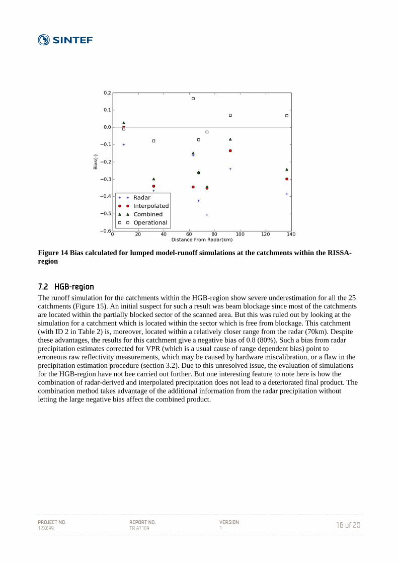
The Nash criterion, correlation coefficient and bias calculated for 8 regulated catchments within the RISSA-region are shown in Figures 12, 13 and 14 respectively. Seven of these catchments (with IDs 11, 12, 13, 14, 18, 20 and 21 in Table 1) belong to TrønderEnergi while the remaining one catchment (with ID 2 in Table 1) belongs to GLB. Aggregated values of the same performance measures for these catchments are presented in Table 4. These aggregated values indicate the average performance across the catchments. Similar to the simulation results with the distributed model, the simulations with the lumped model showed the best performance, on average, with the combined precipitation input. This superiority is reflected by all the three performance measures. Underestimation of runoff is evident, as with the distributed model simulations, for all cases. The runoff simulated using the radar-derived precipitation has the largest bias. The results from the model runs using the operational inputs were not considered in the inter-comparison but have been included for reference purposes. The higher values of the performance measures for the operational input result from the fact that the lumped model has been individually calibrated for each catchment using the same input. Statkraft also ran their lumped model for one of the unregulated catchments in the region, Gaula-Eggafoss (with ID 5 in Table 1). However, the model was ran using only the radar-derived input and the parameters Pcorr and Scorr were set to values higher than 1. Their simulation indicated that this input underestimates runoff. Table 4 Average performance measures of lumped model-runoff simulations for the catchments within the RISSA-region

Precipitation product Nash-Average Corr-Average Bias-Median Radar 0.351 0.670 -0.366 Interpolated 0.524 0.766 -0.298 Combined 0.566 0.787 -0.243 Operational 0.638 0.806 -0.011

PROJECT NO. 12X649.

REPORT NO. TR A7184

VERSION 1

17 of 20

Figure 12 Nash criteria calculated for lumped model-runoff simulations at the catchments within the RISSA-region

Figure 13 Correlation coefficients calculated for lumped model-runoff simulations at the catchments within the RISSA-region

PROJECT NO. 12X649.

REPORT NO. TR A7184

VERSION 1

18 of 20

Figure 14 Bias calculated for lumped model-runoff simulations at the catchments within the RISSA-region

7.2 HGB-region

The runoff simulation for the catchments within the HGB-region show severe underestimation for all the 25 catchments (Figure 15). An initial suspect for such a result was beam blockage since most of the catchments are located within the partially blocked sector of the scanned area. But this was ruled out by looking at the simulation for a catchment which is located within the sector which is free from blockage. This catchment (with ID 2 in Table 2) is, moreover, located within a relatively closer range from the radar (70km). Despite these advantages, the results for this catchment give a negative bias of 0.8 (80%). Such a bias from radar precipitation estimates corrected for VPR (which is a usual cause of range dependent bias) point to erroneous raw reflectivity measurements, which may be caused by hardware miscalibration, or a flaw in the precipitation estimation procedure (section 3.2). Due to this unresolved issue, the evaluation of simulations for the HGB-region have not bee carried out further. But one interesting feature to note here is how the combination of radar-derived and interpolated precipitation does not lead to a deteriorated final product. The combination method takes advantage of the additional information from the radar precipitation without letting the large negative bias affect the combined product.

PROJECT NO. 12X649.

REPORT NO. TR A7184

VERSION 1

19 of 20

Figure 15 Bias calculated for distributed model-runoff simulations at the catchments within the HGB-region

8 Conclusions

Three precipitation products (radar-derived, interpolated and combination of the two) were generated as input for both a distributed and a lumped model. Two regions, each with 25 catchments, were set up for modelling. All the three products were evaluated by comparing the simulated and observed runoff at the catchments within these regions. In order to expose any bias in the precipitation inputs, all model parameters which adjust the input have been set to neutral values. Three assessment criteria were used to measure the performance: Nash criterion, correlation coefficient and bias. Based on the calculated performance measures at each catchment, the following conclusions are drawn:

The simulations with the combined precipitation input give the best performance for both the distributed and the lumped model (excluding the operational inputs). This reveals that the radar-derived and interpolated precipitation complement each other. The combination method takes advantage of the additional information provided by both sources.

All the three products underestimated the simulated runoff. The negative bias in the radar-derived precipitation is probably due to unrepresentative parameters for the Z-R relationship and orographic enhancement of precipitation, which had not been included in the estimation procedure. And the bias in the interpolated precipitation may be probably due to not including correction for rain gauge catch deficit due to wind and also due to orographic effects which go undetected between the gauges.

The radar-derived precipitation estimates give reasonable runoff simulation for the catchments within the RISSA-region. Even though the performance measures for the simulation with the radar-derived input have lower values than the simulations with the interpolated input, its performance cannot be considered to be inferior considering the fact that the models were calibrated using the interpolated precipitation input. What makes the radar-derived estimates even more promising is that they managed to compete with the interpolated precipitation without being subjected to an optimum or region specific parameters for the Z-R relationship. A slight adjustment of these

PROJECT NO. 12X649.

REPORT NO. TR A7184

VERSION 1

20 of 20

parameters, particularly the multiplicative parameter, based on the physics of drop size distribution or comparison with data from disdromters, can lead to better results.

The severe underestimation of the precipitation estimates derived from the Hægebostad radar helped identify one important and useful feature of the combination method used in the project. Although the radar-derived precipitation had a large negative bias, the combination method did not deteriorate the interpolated precipitation. It rather resulted in a better product than the interpolation precipitation by using the additional information from the radar-derived precipitation.

The distributed model was calibrated and run with one parameter set for all the catchments in each region. An important potential of using radar-derived precipitation with a distributed model in the context of regional calibration is simulation of runoff at ungauged catchments.

9 References

Elo, C.A. 2012 Radar data correction procedure Marshall, J.S. and Palmer, W.M.K. 1948 The distribution of raindrops with size. Journal of Meteorology, 5, 165-166. Todini, E. (2001): A Bayesian technique for conditioning radar precipitation estimates to rain-gauge measurements. Hydrology and Earth System Sciences 5 (2), p. 186-199.

Technology for a better society

www.sintef.no