tra c congestion estimation in vehicular ad hoc...
TRANSCRIPT
Traffic Congestion Estimationin
Vehicular Ad Hoc Networks
A thesis submitted in partial fulfillment of the requirementsfor the degree of
Bachelor of Technology (Honours)
in
Computer Science and Engineering
by
Rayman Preet Singh
06CS3023
advised by
Dr. Arobinda Gupta
Department of Computer Science and EngineeringIndian Institute of Technology, Kharagpur
May 2010

Certificate
This is to certify that the thesis entitled Traffic Congestion Estima-
tion in Vehicular Ad Hoc Networks submitted by Rayman Preet Singh
(06CS3023) to the Department of Computer Science and Engineering is a
bonafide record of research work carried out by him under my supervision
and guidance. This thesis has fulfilled all the requirements as per the reg-
ulations of the institute and, in my opinion, has reached or exceeded the
standard needed for submission.
Dr. Arobinda Gupta
Assosiate Professor
Department of Computer Science and Engineering
IIT Kharagpur
May 2010

Acknowledgment
I would like to express my gratitude towards Prof. Arobinda Gupta for
the supervisory role he played to utmost perfection. Taking time out of his
busy schedule, he ensured that the project work was carried out methodically
and meticulously. I especially thank him for his encouragement and his
accurate comments which were of critical importance, and am indebted to
him for extending out all the necessary support throughout the duration of
the project and for being a constant source of inspiration.
I would also like to thank Md. Mozaffar Afaque, Vinu Rajshekhar and
Gourav Khaneja for their invaluable help, guidance and motivation. Their
continuous support and encouragement has played a key role in the comple-
tion of this work.
Rayman Preet Singh
06CS3023
Department of Computer Science and Engineering
IIT Kharagpur
May 2010

Contents
Contents i
1 Introduction 1
1.1 Motivation . . . . . . . . . . . . . . . . . . . . . . . . . . . . . 2
1.2 Contributions . . . . . . . . . . . . . . . . . . . . . . . . . . . 4
1.3 Thesis Overview . . . . . . . . . . . . . . . . . . . . . . . . . . 4
2 Literature Overview 6
2.1 Related Work . . . . . . . . . . . . . . . . . . . . . . . . . . . 6
2.2 Background and Essential Notions . . . . . . . . . . . . . . . . 8
3 Beacon Characterization 10
3.1 Need for Characterization . . . . . . . . . . . . . . . . . . . . 10
3.2 Approach towards solution . . . . . . . . . . . . . . . . . . . . 11
3.3 Beacon Relevance . . . . . . . . . . . . . . . . . . . . . . . . . 13
4 Proposed Algorithm 14
4.1 Classes of Vehicular Congestion . . . . . . . . . . . . . . . . . 14
4.2 Algorithm Description . . . . . . . . . . . . . . . . . . . . . . 15
4.3 Discussion . . . . . . . . . . . . . . . . . . . . . . . . . . . . . 18
i

5 Simulation Study 20
5.1 Simulation Setup . . . . . . . . . . . . . . . . . . . . . . . . . 20
5.2 Parameter Initialization . . . . . . . . . . . . . . . . . . . . . 21
5.3 Performance Evaluation . . . . . . . . . . . . . . . . . . . . . 24
5.4 Experiments . . . . . . . . . . . . . . . . . . . . . . . . . . . . 24
5.4.1 Scenario 1 : Wide moving jam (J) . . . . . . . . . . . . 25
5.4.2 Scenario 2 : Synchronized Traffic Flow . . . . . . . . . 32
5.4.3 Scenario 3 : Low Congestion . . . . . . . . . . . . . . . 39
6 Applications 46
6.1 Application : Information Dissemination . . . . . . . . . . . . 47
6.1.1 Probability based Approach . . . . . . . . . . . . . . . 47
6.1.2 Deterministic Approach Using Vehicular Congestion . . 48
6.1.3 Experiments . . . . . . . . . . . . . . . . . . . . . . . . 49
7 Conclusion 54
7.1 Future Work . . . . . . . . . . . . . . . . . . . . . . . . . . . . 55
ii

Chapter 1
Introduction
A mobile ad hoc network(MANET) is a wireless network consisting of mobile
nodes in which all the network-level activity is carried out by the nodes
themselves, without additional infrastructure support. Each node in such
a network plays the role of a router as well as an end-machine, and hence,
all nodes in the network participate actively in message forwarding. The
network topology is subject to change owing to the mobility in the nature of
the nodes.
Vehicular Ad-Hoc Networks (VANETs) are a special kind of Mobile Ad-
Hoc Networks (MANETs), where wireless-equipped vehicles form the under-
lying network. Communications in mobile ad hoc wireless networks bolsters
various distributed applications among mobile nodes in infrastructure-free
environments. However, characterized by relatively high mobility, communi-
cation in VANETs exhibits stronger challenges than that in any other class
of MANETs.
Among various communication applications in VANETs, there is a wide
range of applications aimed at providing a solution to problems experienced
by commuters due to modern day vehicular traffic. These include appli-
cations involving traffic safety, traffic management and traffic monitoring,
which not only provide for an elevated levels of on-road safety but also maxi-
mize on-road traffic flow leading to an improved driver experience. Commer-
1
Chapter 1: Introduction
cial applications are designed for providing an enhanced user experience, and
include communication and data-sharing applications for providing services
such as Internet access, audio/video streaming solutions etc.
Vehicular traffic congestion is a major problem associated with vehicular
traffic which has been attracting the extensive attention of research in the
field of VANETs. Vehicular congestion estimation shall not only provide a
basis for development of traffic monitoring application but also aid in devel-
opment of other applications which can exploit traffic congestion information
for other goals in VANETs such as disseminating information, suggesting al-
ternate driving route etc.
Although, vehicular congestion is very well defined qualitatively, a definite
quantitative measure for it exists only in terms of features such as average
commuting time, number of vehicles on the road etc. Mobility pattern asso-
ciated with the nodes in VANET bears certain characteristic features, owing
to its large similarity with fluid flow. This traffic flow pattern, coupled with
vehicle-to-vehicle communication in a VANET can be effectively used to de-
tect and estimate vehicular traffic congestion.
1.1 Motivation
Although vehicular traffic and congestion detection and estimation tech-
niques have been studied in much details, there exists a paucity of correlated
study of traffic flow and associated vehicular congestion in the light of Vehicu-
lar Ad Hoc Networks (VANETs). Vehicular traffic congestion is characterized
by the relative presence or absence of certain specific characteristics, but a
fixed measure or metric to represent them effectively is needed for facilitat-
ing congestion estimation in a distributed environment such as VANETs. In
order to develop and employ any such technique suitable for deployment in
VANETs , a demarcating notion of the “condition” of traffic surrounding a
node needs to be defined.
Also, an effective measure of the traffic condition would also allow us to
2

Chapter 1: Introduction
relate it to the state of the wireless network prevalent in any given area of
study, which can be exploited to achieve efficiency of the network governed
by certain network parameters such as channel load, channel availability and
many others. Further, determination of the network condition can, help to
enhance the existent network modality, and, help avoid occurrence of situa-
tions that are hazardous for effective and efficient car to car communications,
whose persistent and equitable state is vital for maintaining a level of vehic-
ular safety on the road.
Being a distributed system, all operations taking place across the VANET,
can be classified into : initial(a node joins the VANET), steady state and ter-
minating(a node leaves the VANET) processes. However, due to the highly
degree of mobility of the nodes only the initial and steady state processes are
of interest, as the duration of communication between two nodes is transitory
and varies across different nodes. Thus, here we concentrate mainly on the
initial and steady state processes, which need to occur at a node for estimat-
ing vehicular congestion in its surrounding. The study and development of a
traffic congestion estimation technique can quite reasonably be divided into
the following parts :
1. Analyzing node mobility and network parameters, along with their as-
sociated pattern of change with network and traffic topology. By dif-
ferentiating traffic and network topology features that are expected
to contribute significantly to any measure or metric(s) of congestion,
we can abstract out the problem of congestion estimation into definite
quantities.
2. Formulating effective and adaptive procedures/protocol(s) that help
measure the vehicular congestion in a distributed way at real-time.
The nodes can then use the measured values to effectively classify their
local ‘view’ of traffic congestion, which is needed for effective sharing
over the VANET and formation of an aggregated picture of congestion.
3. Developing a process for macroscopic measurement and estimation of
vehicular congestion at a global scope, taking into consideration the
3

Chapter 1: Introduction
dynamism of the mobile nodes in the VANET.
The thesis shall investigate all three divisions sequentially.
Note that, in this work we shall assume all nodes (vehicles) to be of non-
malicious nature, and that, all nodes adhere to the procedures/protocol(s)
devised herein.
1.2 Contributions
This thesis presents the following contributions :
1. An approach for classification of surrounding nodes for estimation and
classification of vehicular congestion is presented. The approach utilizes
both the traffic mobility patterns and the network topology character-
istics of a VANET.
2. An algorithm for obtaining the different classes of vehicular conges-
tion at real-time is constructed, and experimental results evaluating its
performance are presented.
3. Information dissemination in VANETs, is presented as an application
of the devised algorithm, and deploys the classes of measured vehic-
ular congestion in a i) probability based approach ii) threshold based
deterministic approach. Further, comparative analysis of performance
is described by means of experimental results.
1.3 Thesis Overview
The thesis is further organized as follows :
• Chapter 2 presents a survey of related work on vehicular congestion
and traffic flow in context of VANETs. Some background, essential
4
Chapter 1: Introduction
notions and system model details relating to our work are also incor-
porated.
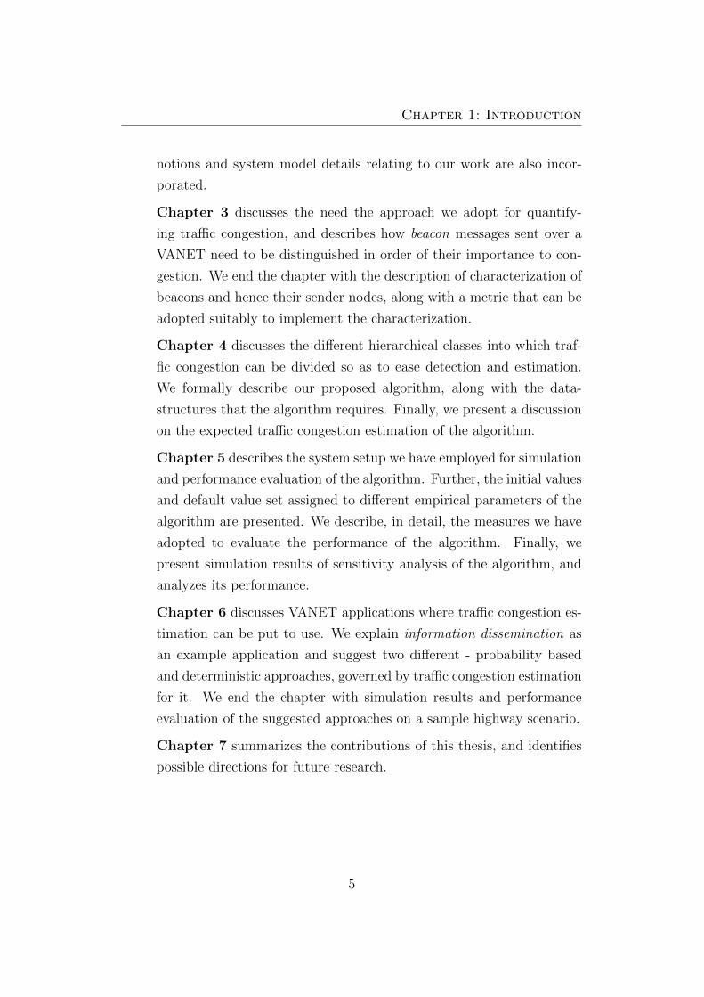
Chapter 3 discusses the need the approach we adopt for quantify-
ing traffic congestion, and describes how beacon messages sent over a
VANET need to be distinguished in order of their importance to con-
gestion. We end the chapter with the description of characterization of
beacons and hence their sender nodes, along with a metric that can be
adopted suitably to implement the characterization.
Chapter 4 discusses the different hierarchical classes into which traf-
fic congestion can be divided so as to ease detection and estimation.
We formally describe our proposed algorithm, along with the data-
structures that the algorithm requires. Finally, we present a discussion
on the expected traffic congestion estimation of the algorithm.
Chapter 5 describes the system setup we have employed for simulation
and performance evaluation of the algorithm. Further, the initial values
and default value set assigned to different empirical parameters of the
algorithm are presented. We describe, in detail, the measures we have
adopted to evaluate the performance of the algorithm. Finally, we
present simulation results of sensitivity analysis of the algorithm, and
analyzes its performance.
Chapter 6 discusses VANET applications where traffic congestion es-
timation can be put to use. We explain information dissemination as
an example application and suggest two different - probability based
and deterministic approaches, governed by traffic congestion estimation
for it. We end the chapter with simulation results and performance
evaluation of the suggested approaches on a sample highway scenario.
Chapter 7 summarizes the contributions of this thesis, and identifies
possible directions for future research.
5

Chapter 2
Literature Overview
This chapter provides a brief insight into some well known vehicular traffic
modelling theories and related research work conducted on them. Further,
we present a brief overview of the mode of communication used in VANETs.
We end this chapter with description of certain essential notions about our
assumed VANET system model.
2.1 Related Work
Being not specific to VANETs, traffic congestion estimation and control has
been widely studied in the past, by mathematically modeling the flow of ve-
hicles. Traffic flow theory by Haberman et al. [1] explores the relationships
among the three main quantities associated with vehicular traffic: vehicle
density, flow and speed. The traffic flow q, measures the number of vehicles
that pass an observer per unit time. The density k, represents the number
of vehicles per unit distance. The speed u, is the distance a vehicle trav-
els per unit time. The units of these quantities are usually expressed in
(veh/sec/lane), (veh/m/lane) and (m/sec) respectively.
Traffic streams are not uniform and vary both over space and time. There-
fore, the quantities q, k and u are meaningful only as averages or as random
6
Chapter 2. Literature Overview
samples of random variables, as has been formalized by Hall et al. [9]. Flow-
Density relationship established in [1] aims to characterize traffic scenarios
into two distinct phases of congested and sparse traffic. This classification,
referred to as the ‘two-phase’ traffic theory, is based on the Fundamental
Traffic flow Relationship [1],
q = u.k (1)
which effectively models the two phases.
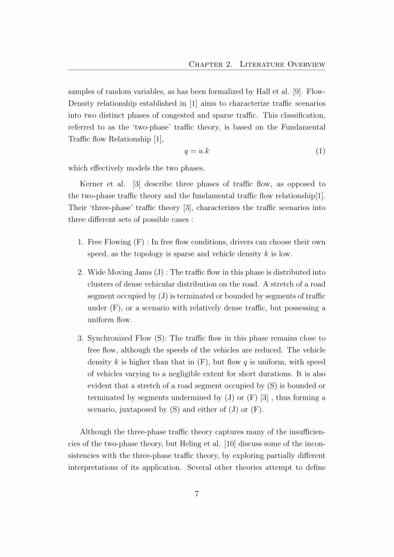
Kerner et al. [3] describe three phases of traffic flow, as opposed to
the two-phase traffic theory and the fundamental traffic flow relationship[1].
Their ‘three-phase’ traffic theory [3], characterizes the traffic scenarios into
three different sets of possible cases :
1. Free Flowing (F) : In free flow conditions, drivers can choose their own
speed, as the topology is sparse and vehicle density k is low.
2. Wide Moving Jams (J) : The traffic flow in this phase is distributed into
clusters of dense vehicular distribution on the road. A stretch of a road
segment occupied by (J) is terminated or bounded by segments of traffic
under (F), or a scenario with relatively dense traffic, but possessing a
uniform flow.
3. Synchronized Flow (S): The traffic flow in this phase remains close to
free flow, although the speeds of the vehicles are reduced. The vehicle
density k is higher than that in (F), but flow q is uniform, with speed
of vehicles varying to a negligible extent for short durations. It is also
evident that a stretch of a road segment occupied by (S) is bounded or
terminated by segments undermined by (J) or (F) [3] , thus forming a
scenario, juxtaposed by (S) and either of (J) or (F).
Although the three-phase traffic theory captures many of the insufficien-
cies of the two-phase theory, but Heling et al. [10] discuss some of the incon-
sistencies with the three-phase traffic theory, by exploring partially different
interpretations of its application. Several other theories attempt to define
7
Chapter 2. Literature Overview
the relationships among each pair of variables in (1), but no single theory
provides the complete picture.
Many studies in VANETs focus on free-flow traffic in their design and
analysis of new protocols (e.g. [12,11,13]). The studies that investigate
connectivity either analytically or using simulations also set the traffic con-
ditions to free flow [15,14]. This choice allows for the greatest flexibility
in controlling each of the vehicle traffic parameters (speed, flow, and den-
sity) independently. However, any vehicular congestion estimation technique
being developed for suitable deployment in modern-day traffic, needs to be
analyzed against an exhaustive set of possible traffic scenarios, and the three-
phase traffic scenario provides the same in a structured and systematic way.
A traffic congestion detection and estimation application is described by
Ghazy et al. [16] and by Padron et al. [17], however these approaches present
congestion detection at a macroscopic level of the VANET, using extensive
collaborative processes amongst the vehicles. Work on congestion estimation
at a global scope by use of locally gathered information has not evolved
as yet. As shall be shown in Chapter 3, the problem of traffic congestion
estimation using VANETs needs to be approached at in a manner different
from that in other typical VANET applications.
2.2 Background and Essential Notions
The mode of communication in VANETs involves broadcast of messages,
on the 5.9Ghz frequency band licensed for VANET applications. We assume
that these broadcast messages are delivered in single-hop, using IEEE 802.11p
(or Dedicated Short Range Communications, DSRC) technology pursued by
industry and governments [18].
In VANETs, there are two types of transmission carried out by nodes:
event-driven messages, whose transmission takes place on the occurance of
certain well-defined events, such as the transmission of safety messages, and
periodic transmissions called beacons used for providing mutual awareness.
8

Chapter 2. Literature Overview
SVA, RHCN and EEBL as described in [4] are some examples of event-driven
messages that are transmitted by nodes, which are used for ensuring safety
of vehicles and also for better coordination among nodes. However, certain
convenience applications also employ event-driven messages. A beacon mes-
sage (denoted BM(v)), is a periodic message broadcasted by each node (‘v’ ),
and contains positional information, speed and direction of movement of the
node, as at the time of broadcast.
9
Chapter 3
Beacon Characterization
3.1 Need for Characterization
As was noted in section 2.2, the two predominant types of transmission car-
ried out by nodes in VANETs are:
1. Event-driven messages, whose transmission is trigerred by the occu-
rance or non-occurance of certain well-defined events at a node. These
comprise mainly of messages relating to on-road vehicle safety.
2. Beacon messages, are periodic transmissions by nodes, containing in-
formation about position and velocity of the node at the time of broad-
cast. They are used for providing mutual-awareness amongst nodes.
Most networking strategies adopted in VANETs, such as routing, transmis-
sion power control, network traffic congestion control etc, follow from tradi-
tional networking protocols. Hence, these networking strategies process all
messages in a similar manner unto the respective classes into which the mes-
sages are divided by them. However in context of detection and estimation
of vehicular congestion, we observe that differentiation amongst messages for
mutual-awareness is required to a great extent, as evident from the following
examples :
10

Chapter 3. Beacon Characterization
1. At any node, beacons received from nodes in a close range, convey more
information with regards to vehicular congestion than the reception of
same number of beacons from any arbitrary set of nodes over the same
fixed time period.
2. A continuous stream of beacons being received at a node would signify
an active link in the network in general, however in context of vehicular
congestion, it is indicative of close proxity of the sender node to the
receiver.
3. A node neighboring another node and bearing a lesser relative velocity
to it is far more likely to be in close proximity to it for a considerable
duration, and hence would be expected to contribute to the vehicular
congestion around the node.
4. Reception of a beacon from a node transmitting at a higher transmis-
sion power signifies that the beacon reaches out to a greater number
of nodes in the vicinity, in effect conveying more vehicular congestion
information to the receiver. This also ensures that the congestion es-
timation strategy is resistant to nodes following different transmission
power control protocols.
Thus, we see that a need for categorizing and characterizing the beacons
in terms of the relevance they bear for estimation of vehicular congestion, is
certain.
3.2 Approach towards solution
Based on the need for classification of beacon messages received at a node,
realized in the preceding section, we present a categorization of beacon mes-
sages. The classification is based on certain characteristics of beacons, inher-
ently based on the fact that any neighboring sender node, would also be the
neighbor for other nodes in a radial distance range, which is at least equal to
the distance between the sender and the node receiving the beacon message.
11
Chapter 3. Beacon Characterization
Senderdistancedv
Transmissionpower levelpv
Relativevelocityvrel
BeaconRelevance
Characterization
Low Low Low Most Relevant True neighborLow High or Low High Not Relevant Passing trafficLow High Low Moderately
RelevantPotential informersabout distant traf-fic.
High High Low Less Relevant Provide informersabout very distanttraffic
High High High Not Relevant Passing TrafficHigh Low High or Low Inconsistent Inconsistent
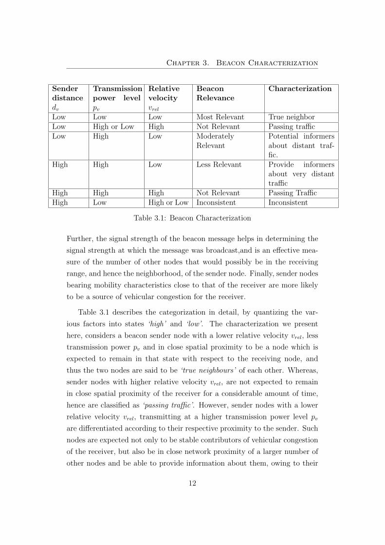
Table 3.1: Beacon Characterization
Further, the signal strength of the beacon message helps in determining the
signal strength at which the message was broadcast,and is an effective mea-
sure of the number of other nodes that would possibly be in the receiving
range, and hence the neighborhood, of the sender node. Finally, sender nodes
bearing mobility characteristics close to that of the receiver are more likely
to be a source of vehicular congestion for the receiver.
Table 3.1 describes the categorization in detail, by quantizing the var-
ious factors into states ‘high’ and ‘low’. The characterization we present
here, considers a beacon sender node with a lower relative velocity vrel, less
transmission power pv and in close spatial proximity to be a node which is
expected to remain in that state with respect to the receiving node, and
thus the two nodes are said to be ‘true neighbours’ of each other. Whereas,
sender nodes with higher relative velocity vrel, are not expected to remain
in close spatial proximity of the receiver for a considerable amount of time,
hence are classified as ‘passing traffic’. However, sender nodes with a lower
relative velocity vrel, transmitting at a higher transmission power level pv
are differentiated according to their respective proximity to the sender. Such
nodes are expected not only to be stable contributors of vehicular congestion
of the receiver, but also be in close network proximity of a larger number of
other nodes and be able to provide information about them, owing to their
12

Chapter 3. Beacon Characterization
higher transmission power level pv. Note that, sender nodes with higher
sender-receiver distance dv, but with a lower transmission power level are
inconsistent in terms of the two parameters and hence not considered for
characterization.
3.3 Beacon Relevance
In order to classify the beacons received at a node, and hence the associated
sender nodes, according to the characterization described above in real-time,
we assign a static weight to each received beacon. This static weight is a
measure of the ‘relevance’ the beacon bears in context of vehicular conges-
tion, and is used by the receiving node to differentiate nodes, according as
their contribution to congestion around it. As noted above the factors which
govern the relevance assigned to each received beacon BM(v), received at a
node u, broadcast by node v, are as follows :
1. The distance dv of the sender v from u,
2. The relative velocity vrel, defined as the magnitude of the relative ve-
locity vector between the sender and the receiver.
3. The transmission power level or signal strength at which the beacon
was broadcast, denoted as pv.
Formally, the relevance of a beaconBM(v) at a node u, denotedRel(BM(v)),
is defined as follows, and holds direct intuitive correlation with the charac-
terization as explained in section 3.2 :
Rel(BM(v)) =pv
vrel × du(2)
13

Chapter 4
Proposed Algorithm
4.1 Classes of Vehicular Congestion
In order to be able to detect and estimate vehicular congestion proficiently,
we classify the traffic congestion experienced at a node u into a set of classes
as follows :
• Instantaneous Congestion : The instantaneous picture of the traffic
in the vicinity at any instant, as perceived by node u. However, speed-
ing/overtaking vehicles are not to be considered as proficient members
of the instantaneous congestion , as they would have little or no con-
tribution to mobility of node u, in the actual present traffic scenario.
• Stabilized Local Congestion : Comprises of the neighboring vehi-
cles of node u, which have been stable members of the instantaneous
congestion at node u, for a considerable amount of time. Thus at any
instant the stabilized local congestion would always be a subset of the
instantaneous congestion.
• Global Congestion : Captures an estimate of the traffic scenario
around node u at a global scope. The estimate is further dependent
upon the stabilized congestion at that instance and the category, (F),
14
Chapter 4. Proposed Algorithm
(J) or (S) into which the present stabilized local congestion falls. We
assume that, an aggregation of local traffic scenarios at nodes in the
stabilized local congestion would be indeed the best possible first degree
estimate for global congestion at node u.
We assert that distribution of vehicular congestion into hierarchical classes,
as above, would aid in systematic measurement of congestion. Since the three
classes describe congestion at successive larger scopes, they can be suitably
combined to present an effective estimate of vehicular congestion surrounding
any node u.
4.2 Algorithm Description
The algorithm aims to characterize the beacons received at any node u by
means of assigning certain static relevance to the message received, as defined
in section 3.3. By means of this algorithm we intend to measure contribution
of congestion towards the different hierarchical classes as specified in the
preceding section.
In accordance with the distributed nature of the VANET system, the
algorithm, as formally described below, provides an autonomous computation
at each node in the network. In order to record the information received with
each beacon, each node maintains a data structure ‘D’, which stores the
content of the received beacon along with the time at which the message was
received. Also, with each such beacon record appended to D, it also stores
the relevance of the beacon. Thus each unit entry in D, can be stereotyped
as:
{Sender ID, Time of receipt, Beacon Relevance}
where, ‘Sender ID’ is the unique identity of the node sending the beacon,
‘Time of receipt’ is the time at which node u acknowledges the receipt of
the beacon, and associates with it its beacon relevance, computed with the
contents of the beacon and present state of the node.
15
Chapter 4. Proposed Algorithm
Algorithm 4.1 Rx BM(BM(v)) : On receipt of beacon BM(v) at node u
Sv ← BM(v).speedXv ← BM(v).positionX
Yv ← BM(v).positionY
~Qv ← BM(v).direction
vrel ← |Sv. ~Qv − Su. ~Qu|dv ←
√(Xv −Xu)2 + (Yv − Yu)2
pv ← BM(v).(signal strength)
Rel(BM(v))← pvvrel × dv
if Rel(BM(v)) ≥ RelTH thenD ← D ∪ {v, t, Rel(BM(v))}
end ifreturn D
Algorithm 4.2 Update(u) : Periodic computation of congestion at node u
for all y ∈ D where y ≡ {yID, yt, yrel} doif (t− yt) > tTH thenD ← D \ {y}
end ifend forcount← count+ 1HD[count]← {D}IC(u)← {D}IDSLC(u)← GetSLC(D, k)GCE(u)← GetGCE(u)return { IC(u) , SLC(u) , GC(u) }
Algorithm 4.3 GetSLC(D,k) : Computation of stabilized local congestion
CD ← φfor j = (count) to (count− k + 1) doCD ← CD ∩HD[j]
end forreturn {CD}ID
16
Chapter 4. Proposed Algorithm
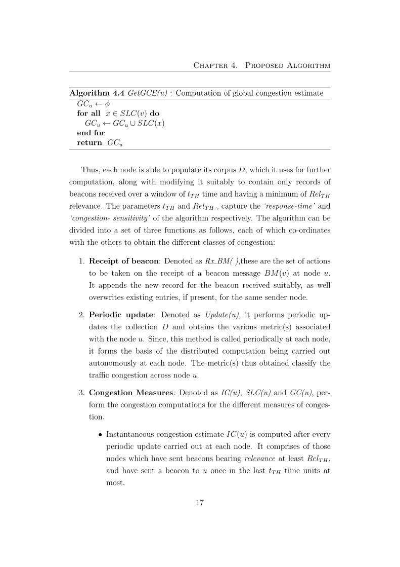
Algorithm 4.4 GetGCE(u) : Computation of global congestion estimate
GCu ← φfor all x ∈ SLC(v) doGCu ← GCu ∪ SLC(x)
end forreturn GCu
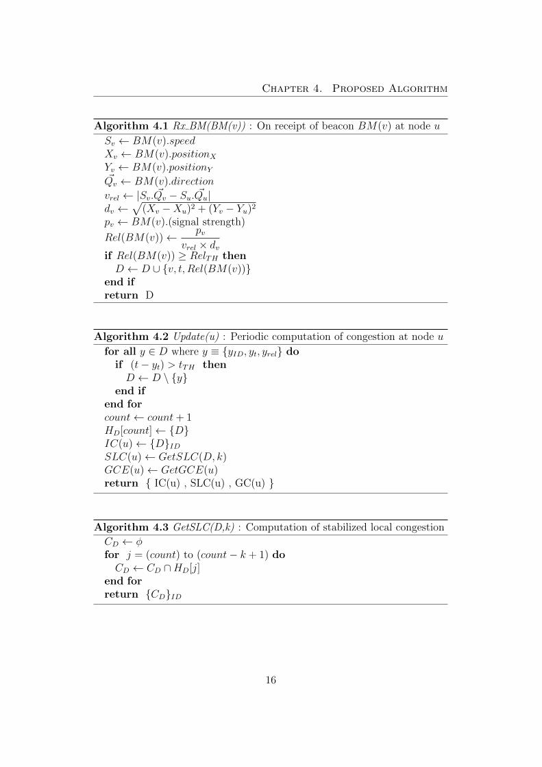
Thus, each node is able to populate its corpus D, which it uses for further
computation, along with modifying it suitably to contain only records of
beacons received over a window of tTH time and having a minimum of RelTH
relevance. The parameters tTH and RelTH , capture the ‘response-time’ and
‘congestion- sensitivity’ of the algorithm respectively. The algorithm can be
divided into a set of three functions as follows, each of which co-ordinates
with the others to obtain the different classes of congestion:
1. Receipt of beacon: Denoted as Rx BM( ),these are the set of actions
to be taken on the receipt of a beacon message BM(v) at node u.
It appends the new record for the beacon received suitably, as well
overwrites existing entries, if present, for the same sender node.
2. Periodic update: Denoted as Update(u), it performs periodic up-
dates the collection D and obtains the various metric(s) associated
with the node u. Since, this method is called periodically at each node,
it forms the basis of the distributed computation being carried out
autonomously at each node. The metric(s) thus obtained classify the
traffic congestion across node u.
3. Congestion Measures: Denoted as IC(u), SLC(u) and GC(u), per-
form the congestion computations for the different measures of conges-
tion.
• Instantaneous congestion estimate IC(u) is computed after every
periodic update carried out at each node. It comprises of those
nodes which have sent beacons bearing relevance at least RelTH ,
and have sent a beacon to u once in the last tTH time units at
most.
17
Chapter 4. Proposed Algorithm
• Stabilized local congestion estimate SLC(u), comprises of nodes
which have been a part of IC(u) for the at least the last k, up-
date steps performed at node u , and measures the set of stable
neighborhood members of u.
• Global congestion estimate GC(u), captures an estimate of the
global traffic scenario across node u. It makes use of one-hop query
and answer messages across neighboring nodes present in SLC(u),
and obtains an aggregation of the stabilized local congestion of
each of the nodes in its present in its stabilized local congestion.
4.3 Discussion
In this section we present a discussion on the expected congestion estimates
as produced by the algorithm in light of the three-phase traffic theory[3]
described briefly in section 2.1. We analyze on a case by case basis the
expected performance on each of the possible traffic flow scenarios :
1. Flowing Jam (J) : In such a scenario, each node is present in highly
dense traffic and neighboring nodes have similar mobility leading to
a similarity between the instantaneous and stabilized local congestion
estimate. Also, the global congestion estimate is expected to produce
a substantially enhanced view of the local congestion as neighboring
nodes are expected to be in similar congestion conditions.
2. Synchronized Flow(S) : The stabilized local congestion estimate is ex-
pected to be lower than the instantaneous congestion, owing to presence
of passing traffic. Since the global congestion estimate would compute
a macroscopic view it is expected to produce a distribution of nodes
connected by local-stable congestion relationship.
3. Free Flow (F) : As the traffic is sparse , the reported local congestion
estimate is equivalent to the instantaneous congestion . Since negligi-
ble amounts of passing traffic exists in such a scenario, the connected
18

Chapter 4. Proposed Algorithm
neighbor set is expected to be stable with time and space.
4. Transition between (S → J) : Although the instantaneous congestion
would be high as compared to the stabilized local congestion, a gradual
stabilization of nodes from instantaneous to stabilized local congestion
is expected, that is an increase in the stabilized local congestion. Such
a scenario is characterized by EEBL message disseminations[4], and
their receipt can be utilized to normalize the congestion computation,
in order to better cope with the changing scenario. Similarly for a
J → S transition, although the stabilized local congestion values are
expected to be higher , but an upfront S scenario would take some time
to provide the correct congestion estimate , until which the node would
assume itself to be in congested traffic but for a duration, depending
upon the parameter tTH .
5. Transition between (F → S) : In such a case, the instantaneous and
stabilized local congestion would be a smaller set of nodes that have
been in close proximity of the reference node, also causing the global
congestion estimate to be similar, and hence an accurate global conges-
tion estimate of the upfront traffic (S), does not seem to appear. Such
a scenario is characterized by an increase by both in instantaneous
and stabilized congestion with time and SVA / RHCN messages[4] are
expected to be disseminated by the upfront nodes, present in the rela-
tively denser traffic.
Note that, computation of the stabilized local congestion GetSLC(), is a
terminating computation over the set HD, which is defined as history of the
set of stabilized local congestion.The computation involves comparison of
the last k versions of stabilized local congestion obtained at previous update
events. Similarly, computations performed on receipt of every beacon mes-
sage Rx BM(), and periodic events to update congestion across the node u,
are also bounded computations. Similarly, getGCE() computes a bounded
set, which is an aggregation over the stable neighbor set and thus its com-
putation is bounded as well.
19

Chapter 5
Simulation Study
5.1 Simulation Setup
The network simulator employed in the experiments is NS[7]-version 2.28,
and VANET Mobisim[8]-version 1.1 is used as the traffic simulator to simu-
late the dynamic traffic scenario and mobility patterns of the vehicles. The
movement pattern of the vehicles, generated by the traffic simulator, in terms
of the current position, speed and direction, is fed into the network simulator,
used to simulate the associated dynamic network topology over the VANET
at real time. This process is automated by means of a data-pipe between
the two simulators and a server-client, two-way communication takes place
between the traffic and network simulators which synchronize the flow of
data amongst themselves and run in parallel at run time. The detailed spec-
ification and implementation of this integrated simulator can be found in
[19].
The network simulator effectively simulates the characteristic mobility
pattern of moving traffic by periodically seeking position and velocity data
of each node from the traffic simulator. The value of this periodic time step,
VMStime−interval , is kept appropriately “small” so as to effectively report
movement and changes in the movement pattern of a node to the network
simulator without substantial delay, and is commensurate to the granularity
20

Chapter 5. Simulation Study
Channel : WirelessPropagation : Two Ray GroundMac : Mac/802 11Queue : Drop Tail / Priority QueueAntenna : Omni Antenna (Ht. 1.5m)Transmission Power : 0.2818dBm (250m)Frequency : 914 Hz
Table 5.1: Network parameters
of the latter. All nodes in a scenario being studied, are associated with a sin-
gle “node group” and hence the update process of their position and velocity
for all nodes is done concurrently with little time-lag. Also, in accordance
with the beaconing model of communication in VANETs, each node sends
out periodic beacons, consisting of its most recent position and velocity, and
are notably used for mutual awareness. Since, the time granularity of the
simulation is indeed VMStime−interval , the beacon interval is always equal or
a multiple of it. The other network parameters are summarized in table-5.1.
5.2 Parameter Initialization
The time interval at which the updated position and velocities of the nodes
are read by the network simulator, VMStime−interval, is set to 1 second, and all
other algorithm parameters are varied, measured and studied in its respect.
Hence, the absolute values of the parameters bear little significant and all
analysis and performance evaluation of the algorithm is conducted by varying
parameters in multiples of VMStime−interval. This also contributes to the fact
that the results are independent of the absolute values of parameters, since
a change in the value of VMStime−interval, would just indicate a changed
granularity of the observed mobility pattern of the vehicles, as perceived by
the network simulator followed by an associated increase in the number of
beacons and other network-related events occurring in the VANET.
21
Chapter 5. Simulation Study
The parameters associated with the algorithm are as follows :
1. Beacon Period (Bp) : The time interval between successive beacon
events occurring at given node. To ensure homogeneity in the VANET,
without loss of generality, it is assumed to be the same for all nodes in
a given traffic scenario.
2. Update Period (Up) : The time interval between successive and periodic
execution of Update(u) at a node, which is assumed to be same for all
the nodes in a given traffic scenario. It can also be defined as the
time-frequency of “updation” of vehicular congestion estimates.
3. Threshold Time (tTH) : At any node u, the maximum amount of time
difference between the current time and the time of receipt of the last
beacon from any neighboring node v, which is reported in the instan-
taneous congestion (IC) at node u.
4. Window Size (K) : At any node u, the number of most recent successive
instances of the instantaneous congestion (IC), which need to contain a
node v which is reported as a member of the stabilized local congestion
(SLC) at node u.
5. Threshold Relevance (RelTH) : The minimum amount of relevance a
beacon needs to possess in order for the corresponding sender node to
be considered, as a member of the instantaneous congestion (IC) and,
hence a potential member of the stabilized local congestion(SLC).
6. Total number of nodes (n) : The total number of nodes in the given
scenario. All results are averaged over the entire set of nodes in the
scenario.
An empirical value ‘α’ of RelTH is calculated as follows :
At any node u, let BM(v) be a beacon message received from a sender node
v, hence Relevance of the beacon Rel(BM(v)), as defined in section 3.3 is,
Rel(BM(v)) =pv
(vrel + δ)× dv
22

Chapter 5. Simulation Study
VMStime−interval : 1 secBeacon period (Bp) : 5 secThreshold time (tTH) : 20 secRelTH : 0.0022544Update period (Up) : 15 secWindow Size (K) : 3
Table 5.2: Default values of parameters
Note that, we augment a constant factor δ here, so as to counter cases of
neighboring nodes moving with same or negligibly different speeds. In order
to obtain RelTH , we assign values to pv, vrel and dv :
pv = 0.2818dBm (3)
(Corresponding to a transmission range of 250m, and assumed equal for all
nodes).
vrel = 1m/sec (4)
(Corresponding to a distance of 5m, which a car would cover relative to
another, and is equal to the assumed length of the vehicle).
dv = 125m (5)
(Assuming any vehicle should be within at least half the transmission range
of another node in order to be a contributor for vehicular congestion at that
node).
Therefore, using (2),
α =0.2818
1× 125= 0.0022544 dBm/m2/s. (5)
The parameters ‘default’ values for these parameters chosen are shown in
table-5.2.
23
Chapter 5. Simulation Study
5.3 Performance Evaluation
For both the stabilized local congestion(SLC) and instantaneous congestion
(IC), two performance measures are studied, namely Precision and Recall of
the reported congestion, defined as follows :
1. Precision : The percentage of nodes in the reported congestion (IC
or SLC) of any node u, which would produce a beacon with relevance
greater than RelTH with respect to node u, if they were to send one
beacon message each to u at the instant at which the vehicular conges-
tion (being evaluated), was reported.
For any node u, let ε denote the set of all the nodes within its transmis-
sion range, which would produce a beacon with relevance greater than
RelTH with respect to any node u, if they were to send a beacon to u
at the instant at which the set is computed. The number of nodes in
ε is denoted by |ε|. Similarly, let ϕ be the set of nodes in the reported
congestion. Note that, ϕ will be equal to either SLC or IC. The number
of nodes in ϕ is denoted by |ϕ|. Therefore,
2. Recall : The fraction|ϕ||ε|
, expressed in percent.
Note that, these measures are studied for both the stabilized local and
instantaneous congestion, and their variation with other factors inherent in
the algorithm, as well as the total number of vehicles, in the traffic scenario
under observation.
In order to analyze the Global Congestion(GC) estimate, the distribution the
average cardinality of the reported Global Congestion(GC), with respect to
the fraction of the total nodes in the scenario is studied.
5.4 Experiments
Three traffic scenarios are considered for the simulation study of the algo-
rithm, each of which corresponds to Synchronized Flow(S), Wide Moving
24
Chapter 5. Simulation Study
Jam(J) and Free Flowing(F) traffic. However, due to the dynamics of the
traffic at run time, transitional traffic scenarios, namely, S→J and S→F, are
also analyzed. An average case analysis is done by averaging the observables
over all nodes present in the scenario. Also, each scenario is evaluated at two
values of the total number of nodes, in order to ensure consistency in the
average case analysis. Presented below are run-time snapshots of the traffic
scenarios considered for the performance evaluation followed by which the
study of the precision and recall for the scenarios as well as their sensitivity
analysis with respect to other variables.
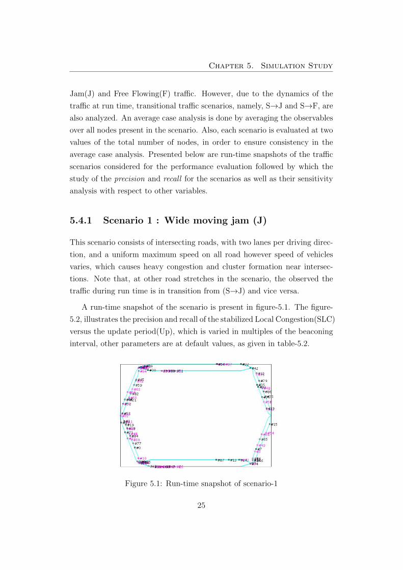
5.4.1 Scenario 1 : Wide moving jam (J)
This scenario consists of intersecting roads, with two lanes per driving direc-
tion, and a uniform maximum speed on all road however speed of vehicles
varies, which causes heavy congestion and cluster formation near intersec-
tions. Note that, at other road stretches in the scenario, the observed the
traffic during run time is in transition from (S→J) and vice versa.
A run-time snapshot of the scenario is present in figure-5.1. The figure-
5.2, illustrates the precision and recall of the stabilized Local Congestion(SLC)
versus the update period(Up), which is varied in multiples of the beaconing
interval, other parameters are at default values, as given in table-5.2.
Figure 5.1: Run-time snapshot of scenario-1
25

Chapter 5. Simulation Study
50
60
70
80
90
100
0 1 2 3 4 5 6 7 8 9 10 11
Pre
cisi
on(in
per
cent
) of
SLC
Update Period(in multiples of Beacon period)
Precision(in percent) of SLC v/s Update period
n=100n=50
0
20
40
60
80
100
0 1 2 3 4 5 6 7 8 9 10 11
Rec
all(i
n pe
r ce
nt)
of S
LC
Update Period(in multiples of Beacon period)
Recall(in per cent) of SLC v/c Update Period
n=100n=50
Figure 5.2: Precision and Recall of the Stabilized Local Congestion(SLC)versus the Update period for scenario-1
26
Chapter 5. Simulation Study
We see that the measured precision increases dominantly as the update period
is increased. This is attributed to the fact that, as more and more time is
allocated for the congestion to converge, its accuracy is bound to increase.
Similarly, the measured recall decreases with update period, owing to the
fact that with the increased time allocated for convergence of congestion,
newer nodes may enter the congestion and be un-reported due to the lesser
time spent in vicinity of the given node, with respect to which evaluation is
performed. However, in the given traffic scenario which is clustered in nature,
there exist certain vehicles which tend to be part of different clusters over
time, and thus if reported as a member of congestion, they are liable to be in a
different cluster at the time of performance evaluation, and hence result in the
corresponding decrease in measured precision. Likewise, a similar behavior
of occurrence of anomalies is also observed in the variation of recall.
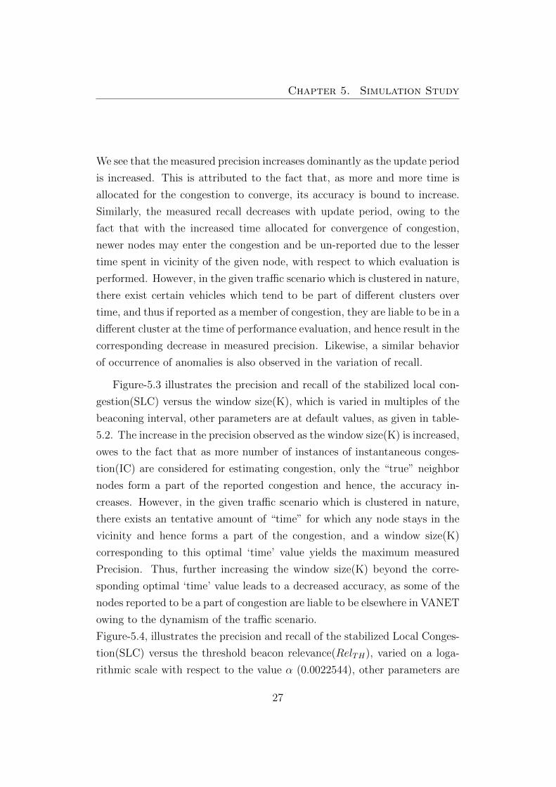
Figure-5.3 illustrates the precision and recall of the stabilized local con-
gestion(SLC) versus the window size(K), which is varied in multiples of the
beaconing interval, other parameters are at default values, as given in table-
5.2. The increase in the precision observed as the window size(K) is increased,
owes to the fact that as more number of instances of instantaneous conges-
tion(IC) are considered for estimating congestion, only the “true” neighbor
nodes form a part of the reported congestion and hence, the accuracy in-
creases. However, in the given traffic scenario which is clustered in nature,
there exists an tentative amount of “time” for which any node stays in the
vicinity and hence forms a part of the congestion, and a window size(K)
corresponding to this optimal ‘time’ value yields the maximum measured
Precision. Thus, further increasing the window size(K) beyond the corre-
sponding optimal ‘time’ value leads to a decreased accuracy, as some of the
nodes reported to be a part of congestion are liable to be elsewhere in VANET
owing to the dynamism of the traffic scenario.
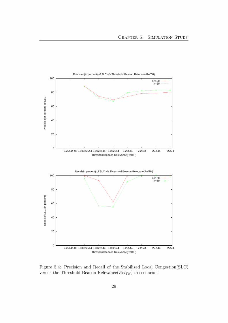
Figure-5.4, illustrates the precision and recall of the stabilized Local Conges-
tion(SLC) versus the threshold beacon relevance(RelTH), varied on a loga-
rithmic scale with respect to the value α (0.0022544), other parameters are
27
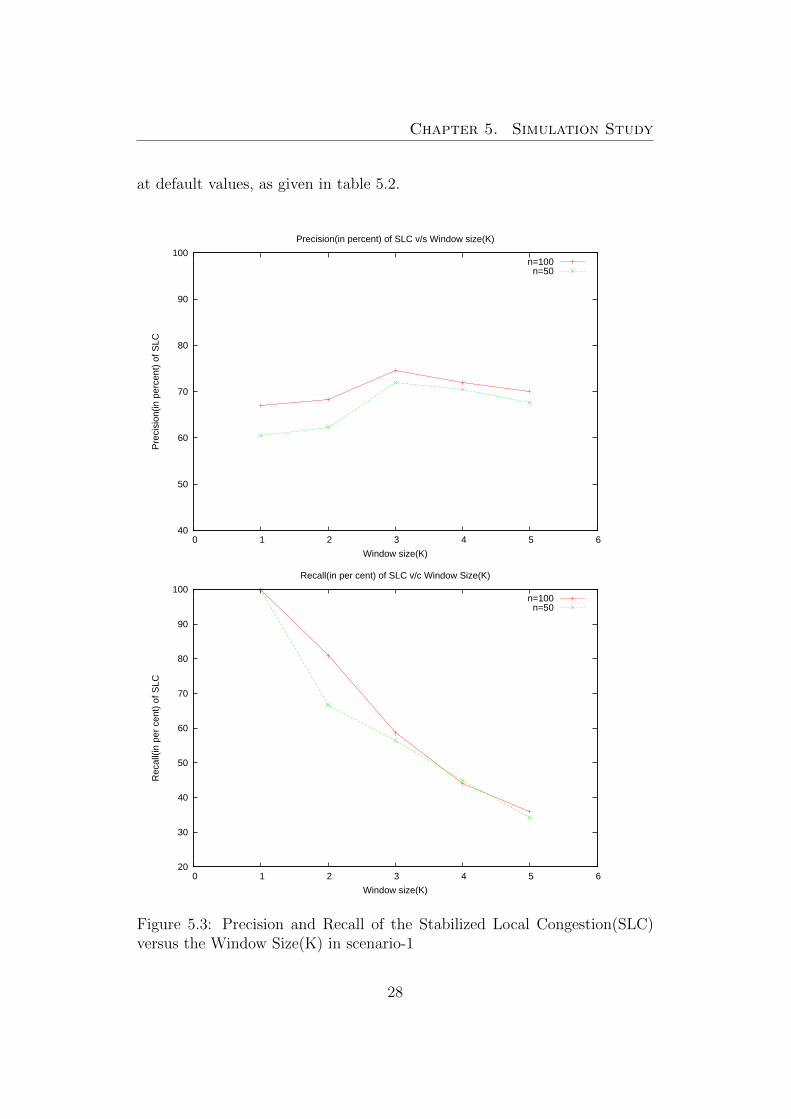
Chapter 5. Simulation Study
at default values, as given in table 5.2.
40
50
60
70
80
90
100
0 1 2 3 4 5 6
Pre
cisi
on(in
per
cent
) of
SLC
Window size(K)
Precision(in percent) of SLC v/s Window size(K)
n=100n=50
20
30
40
50
60
70
80
90
100
0 1 2 3 4 5 6
Rec
all(i
n pe
r ce
nt)
of S
LC
Window size(K)
Recall(in per cent) of SLC v/c Window Size(K)
n=100n=50
Figure 5.3: Precision and Recall of the Stabilized Local Congestion(SLC)versus the Window Size(K) in scenario-1
28
Chapter 5. Simulation Study
0
20
40
60
80
100
2.2544e-05 0.00022544 0.0022544 0.022544 0.22544 2.2544 22.544 225.4
Pre
cisi
on(in
per
cent
) of
SLC
Threshold Beacon Relevance(RelTH)
Precision(in percent) of SLC v/s Threshold Beacon Relecane(RelTH)
n=100n=50
0
20
40
60
80
100
2.2544e-05 0.00022544 0.0022544 0.022544 0.22544 2.2544 22.544 225.4
Rec
all o
f SLC
(in
per
cent
)
Threshold Beacon Relevance(RelTH)
Recall(in percent) of SLC v/s Threshold Beacon Relecane(RelTH)
n=100n=50
Figure 5.4: Precision and Recall of the Stabilized Local Congestion(SLC)versus the Threshold Beacon Relevance(RelTH) in scenario-1
29

Chapter 5. Simulation Study
Clearly, both the precision and recall are expected to increase as the thresh-
old relevance(RelTH) is increased, and the same is observed as well. How-
ever, as threshold relevance(RelTH) is decreased (on the logarithmic scale),
the measured precision and recall increases because a very low threshold
relevance(RelTH) causes all nodes in the vicinity to be reported in the con-
gestion, as any given beacon is bound to possess a relevance greater than such
a low value of threshold relevance(RelTH). And because the evaluation of
precision and recall considers only the nodes in the vicinity of the given node,
it leads to a pseudo-increase in the measure values. Note that, there exists
considerable difference in the recall values for the two sets of nodes, because
a increased number of nodes increases the vehicle-density in the scenario.
Figure-5.5 presents the distribution of the number of nodes reported in
the global congestion(GC) with respect to the fraction of nodes.
0
0.05
0.1
0.15
0.2
0.25
0.3
2 3 4 5 6 7 8 9 10 11 12 13 14 15 16 17 18
Fra
ctio
n of
Nod
es
Number of nodes in GC
(Fraction of nodes) v/s (Number of Nodes in GC)
n=50n=100
Figure 5.5: Distribution of the number of nodes reported in the Global Con-gestion(GC) in scenario-1
30

Chapter 5. Simulation Study
It is evident that for the given two sets of nodes, for which the analysis is
conducted, a greater number of nodes(n=100), leads to a more sparse dis-
tribution, as compared to the case where number of nodes is lower(n=50),
which has a uniform but dense distribution. Also, the occurrence of peaks (in
fraction of nodes) at certain number of nodes in global congestion(GC), re-
lates to the ‘clustered’ nature of the traffic in the given scenario, where traffic
occurs in clusters juxtaposed by free-flowing or moderately dense traffic.
The variation of Precision of the instantaneous congestion(IC) with the
update period and threshold relevance(RelTH) respectively, is presented in
figures-5.6 and 5.7 respectively.
50
60
70
80
90
100
0 1 2 3 4 5 6 7 8 9 10 11
Pre
cisi
on(in
per
cent
) of
IC
Update Period(in multiples of Beacon period)
Precision(in percent) of IC v/s Update period
n=100n=50
Figure 5.6: Variation of Precision of the Instantaneous Congestion(IC) withthe Update period in scenario-1
31

Chapter 5. Simulation Study
0
20
40
60
80
100
2.2544e-05 0.00022544 0.0022544 0.022544 0.22544 2.2544 22.544 225.4
Pre
cisi
on(in
per
cent
) of
IC
Threshold Beacon Relevance(RelTH)
Precision(in percent) of IC v/s Threshold Beacon Relevance(RelTH)
n=100n=50
Figure 5.7: Variation of Precision of the Instantaneous Congestion(IC) withThreshold Relevance(RelTH) in scenario-1
5.4.2 Scenario 2 : Synchronized Traffic Flow
This scenario consists of intersections which are juxtaposed with connecting
roads with greatly varying maximum speed limits and two lanes per driving
direction. The roads with lower speed limits are shorter in length and cause
a bottleneck in the traffic merging from higher speed limit roads, leading to
the formation of a synchronized flow of traffic. Note that, the scenario also
encompasses a transition of traffic from (S→F) and vice versa, owing to vast
stretch of higher speed limit roads.
A run-time snapshot of the scenario is present in figure-5.8. The figures-
5.9 and 5.10, illustrate the precision and recall of the stabilized local con-
gestion(SLC) versus the update period, which is varied in multiples of the
beaconing interval, other parameters are at default values, as given in table
5.2.
32

Chapter 5. Simulation Study
Figure 5.8: Run-time snapshot of the scenario-2
50
60
70
80
90
100
0 1 2 3 4 5 6 7 8 9 10 11
Pre
cisi
on(in
per
cent
) of
SLC
Update Period(in multiples of Beacon period)
Precision(in percent) of SLC v/s Update period
n=100n=50
Figure 5.9: Precision of the Stabilized Local Congestion(SLC) versus theUpdate period in scenario-2
33

Chapter 5. Simulation Study
0
20
40
60
80
100
0 1 2 3 4 5 6 7 8 9 10 11
Rec
all(i
n pe
r ce
nt)
of S
LC
Update Period(in multiples of Beacon period)
Recall(in per cent) of SLC v/c Update Period
n=100n=50
Figure 5.10: Recall of the Stabilized Local Congestion(SLC) versus the Up-date period in scenario-2
The explanation for this variation is similar to the corresponding variation in
scenario 1. However, it is observed that the deviation of anomalies from the
expected behavior is reduced as compared to scenario-1, which is attributed
to the reduced clustered topology of the traffic in the given scenario, which
is dominated by a synchronized flow of traffic.
In this type of scenario, owing to no distinct formation of active clusters
of traffic at run-time, there does not exist an tentative value of “time” a node
spends in the vicinity of another, due to which we observe that the precision
value increases with increased window size(K). Likewise, the recall value
decreases because a greater window size leads to the exclusion of “newer”
nodes from the reported congestion, thereby recall decreases with window
size(K). Figure-5.11 presents the associated variation.
34

Chapter 5. Simulation Study
40
50
60
70
80
90
100
0 1 2 3 4 5 6
Pre
cisi
on(in
per
cent
) of
SLC
Window size(K)
Precision(in percent) of SLC v/s Window size(K)
n=100n=50
0
20
40
60
80
100
0 1 2 3 4 5 6
Rec
all(i
n pe
r ce
nt)
of S
LC
Window size(K)
Recall(in per cent) of SLC v/c Window Size(K)
n=100n=50
Figure 5.11: Precision and Recall of the Stabilized Local Congestion(SLC)versus the Window Size(K) in scenario-2
35

Chapter 5. Simulation Study
The figures-5.11 and 5.12, illustrate the precision and recall of the stabi-
lized local congestion(SLC) versus the threshold beacon relevance(RelTH),
varied on a logarithmic scale with respect to the value α (0.0022544), other
parameters are at default values, as given in table-5.2.
0
20
40
60
80
100
2.2544e-05 0.00022544 0.0022544 0.022544 0.22544 2.2544 22.544 225.4
Pre
cisi
on(in
per
cent
) of
SLC
Threshold Beacon Relevance(RelTH)
Precision(in percent) of SLC v/s Threshold Beacon Relevance(RelTH)
n=100n=50
Figure 5.12: Precision of the Stabilized Local Congestion(SLC) versus theThreshold Beacon Relevance(RelTH) in scenario-2
Although the variation follows similar trend, as in case of the corresponding
variation in scenario-1, however, a greater difference is observed in the pre-
cision and recall values of the two node sets because a two-fold increase in
the number of nodes increases the vehicle-density in the synchronized flow
scenario and affects the traffic topology more adversely, leading to cluster-
formation in the scenario and consequent fall in the Precision and Recall
values.
36

Chapter 5. Simulation Study
0
20
40
60
80
100
2.2544e-05 0.00022544 0.0022544 0.022544 0.22544 2.2544 22.544 225.4
Rec
all o
f SLC
(in
per
cent
)
Threshold Beacon Relevance(RelTH)
Recall(in percent) of SLC v/s Threshold Beacon Relecane(RelTH)
n=100n=50
Figure 5.13: Recall of the Stabilized Local Congestion(SLC) versus theThreshold Beacon Relevance(RelTH) in scenario-2
Corresponding to figure-5.5, figure-5.14 presents the distribution of the num-
ber of nodes reported in the global congestion(GC) with respect to the frac-
tion of total nodes in the scenario. A more sparse distribution of the number
of nodes in the global congestion(GC), is evidently observed due to the traf-
fic topology in the scenario which is more uniformly distributed as compared
to clustered traffic and hence, equal size peaks are observed at different val-
ues, corresponding to the relative positions of nodes in a bottleneck-traffic
environment.
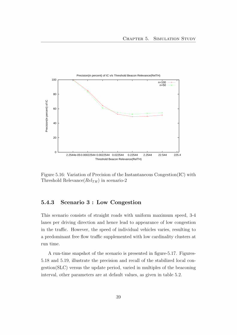
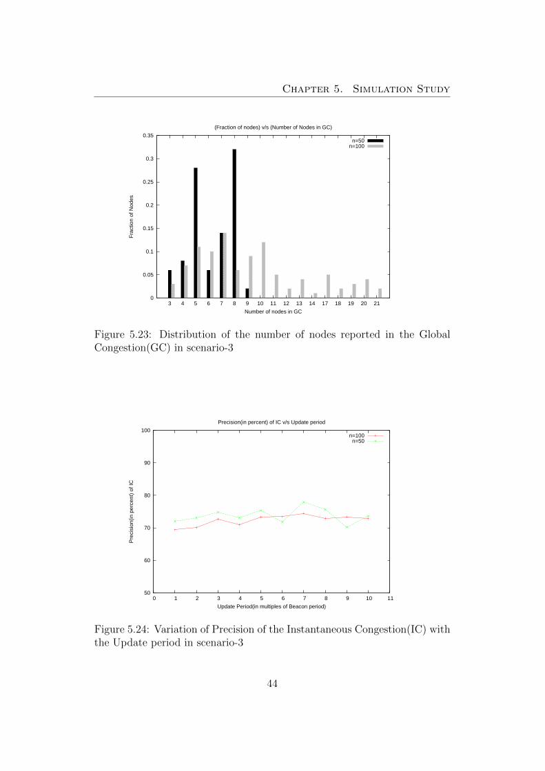
Finally, the variation of Precision of the instantaneous congestion(IC)
with the update period and threshold relevance(RelTH) respectively, is pre-
sented in figures-5.15 and 5.16. Similar to the variation observed in the stabi-
lized local congestion(SLC), the measure precision increases with the update
Period, and characteristic presence of anomalies is also observed. Note that,
the gradient of increase in lower in case of instantaneous congestion(IC).
37

Chapter 5. Simulation Study
0
0.05
0.1
0.15
0.2
0.25
0.3
0.35
0.4
4 6 7 8 9 10 11 12 13 14 15 16 17 18 19 20
Fra
ctio
n of
Nod
es
Number of nodes in GC
(Fraction of nodes) v/s (Number of Nodes in GC)
n=50n=100
Figure 5.14: Distribution of the number of nodes reported in the GlobalCongestion(GC) in scenario-2
50
60
70
80
90
100
0 1 2 3 4 5 6 7 8 9 10 11
Pre
cisi
on(in
per
cent
) of
IC
Update Period(in multiples of Beacon period)
Precision(in percent) of IC v/s Update period
n=100n=50
Figure 5.15: Variation of Precision of the Instantaneous Congestion(IC) withthe Update period in scenario-2
38
Chapter 5. Simulation Study
0
20
40
60
80
100
2.2544e-05 0.00022544 0.0022544 0.022544 0.22544 2.2544 22.544 225.4
Pre
cisi
on(in
per
cent
) of
IC
Threshold Beacon Relevance(RelTH)
Precision(in percent) of IC v/s Threshold Beacon Relevance(RelTH)
n=100n=50
Figure 5.16: Variation of Precision of the Instantaneous Congestion(IC) withThreshold Relevance(RelTH) in scenario-2
5.4.3 Scenario 3 : Low Congestion
This scenario consists of straight roads with uniform maximum speed, 3-4
lanes per driving direction and hence lead to appearance of low congestion
in the traffic. However, the speed of individual vehicles varies, resulting to
a predominant free flow traffic supplemented with low cardinality clusters at
run time.
A run-time snapshot of the scenario is presented in figure-5.17. Figures-
5.18 and 5.19, illustrate the precision and recall of the stabilized local con-
gestion(SLC) versus the update period, varied in multiples of the beaconing
interval, other parameters are at default values, as given in table 5.2.
39

Chapter 5. Simulation Study
Figure 5.17: Run-time snapshot of scenario-3
50
60
70
80
90
100
0 1 2 3 4 5 6 7 8 9 10 11
Pre
cisi
on(in
per
cent
) of
SLC
Update Period(in multiples of Beacon period)
Precision(in percent) of SLC v/s Update period
n=100n=50
Figure 5.18: Precision of the Stabilized Local Congestion(SLC) versus theUpdate period in scenario-3
40

Chapter 5. Simulation Study
0
20
40
60
80
100
0 1 2 3 4 5 6 7 8 9 10 11
Rec
all(i
n pe
r ce
nt)
of S
LC
Update Period(in multiples of Beacon period)
Recall(in per cent) of SLC v/c Update Period
n=100n=50
Figure 5.19: Recall of the Stabilized Local Congestion(SLC) versus the Up-date period in scenario-3
40
50
60
70
80
90
100
0 1 2 3 4 5 6
Pre
cisi
on(in
per
cent
) of
SLC
Window size(K)
Precision(in percent) of SLC v/s Window size(K)
n=100n=50
Figure 5.20: Precision of the Stabilized Local Congestion(SLC) versus theWindow Size(K) in scenario-3
41
Chapter 5. Simulation Study
20
30
40
50
60
70
80
90
100
0 1 2 3 4 5 6
Rec
all(i
n pe
r ce
nt)
of S
LC
Window size(K)
Recall(in per cent) of SLC v/c Window Size(K)
n=100n=50
Figure 5.21: Recall of the Stabilized Local Congestion(SLC) versus the Win-dow Size(K) in scenario-3
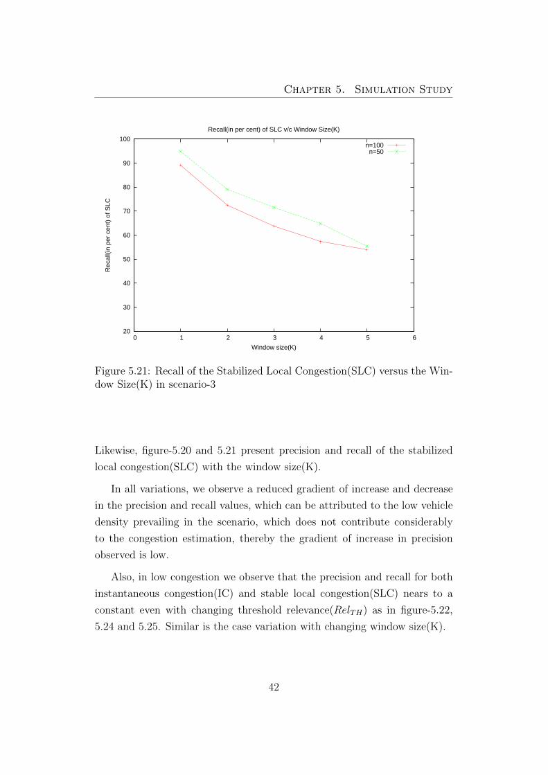
Likewise, figure-5.20 and 5.21 present precision and recall of the stabilized
local congestion(SLC) with the window size(K).
In all variations, we observe a reduced gradient of increase and decrease
in the precision and recall values, which can be attributed to the low vehicle
density prevailing in the scenario, which does not contribute considerably
to the congestion estimation, thereby the gradient of increase in precision
observed is low.
Also, in low congestion we observe that the precision and recall for both
instantaneous congestion(IC) and stable local congestion(SLC) nears to a
constant even with changing threshold relevance(RelTH) as in figure-5.22,
5.24 and 5.25. Similar is the case variation with changing window size(K).
42

Chapter 5. Simulation Study
0
20
40
60
80
100
2.2544e-05 0.00022544 0.0022544 0.022544 0.22544 2.2544 22.544 225.4
Pre
cisi
on(in
per
cent
) of
SLC
Threshold Beacon Relevance(RelTH)
Precision(in percent) of SLC v/s Threshold Beacon Relevance(RelTH)
n=100n=50
0
20
40
60
80
100
2.2544e-05 0.00022544 0.0022544 0.022544 0.22544 2.2544 22.544 225.4
Rec
all o
f SLC
(in
per
cent
)
Threshold Beacon Relevance(RelTH)
Recall(in percent) of SLC v/s Threshold Beacon Relecane(RelTH)
n=100n=50
Figure 5.22: Precision and Recall of the Stabilized Local Congestion(SLC)versus the Threshold Beacon Relevance(RelTH) in scenario-3
43
Chapter 5. Simulation Study
0
0.05
0.1
0.15
0.2
0.25
0.3
0.35
3 4 5 6 7 8 9 10 11 12 13 14 17 18 19 20 21
Fra
ctio
n of
Nod
es
Number of nodes in GC
(Fraction of nodes) v/s (Number of Nodes in GC)
n=50n=100
Figure 5.23: Distribution of the number of nodes reported in the GlobalCongestion(GC) in scenario-3
50
60
70
80
90
100
0 1 2 3 4 5 6 7 8 9 10 11
Pre
cisi
on(in
per
cent
) of
IC
Update Period(in multiples of Beacon period)
Precision(in percent) of IC v/s Update period
n=100n=50
Figure 5.24: Variation of Precision of the Instantaneous Congestion(IC) withthe Update period in scenario-3
44

Chapter 5. Simulation Study
0
20
40
60
80
100
2.2544e-05 0.00022544 0.0022544 0.022544 0.22544 2.2544 22.544 225.4
Pre
cisi
on(in
per
cent
) of
IC
Threshold Beacon Relevance(RelTH)
Precision(in percent) of IC v/s Threshold Beacon Relevance(RelTH)
n=100n=50
Figure 5.25: Variation of Precision of the Instantaneous Congestion(IC) withThreshold Relevance(RelTH) in scenario-3
The variation of the distribution of the global congestion(GC) is observed to
be lesser than that in the case of scenario-1 and scenario-2.
45
Chapter 6
Applications
We believe that the stabilized local congestion estimate as computed by the
algorithm can be put to use in many applications, such as beacon frequency
control and transmission power control , as suggested by Torrent-Moreno in
[5], dynamic transmission power assignment to nodes can also be used to
control vehicular congestion.
Vehicular congestion can also be used in an application of trust building
notions among the nodes, so as to make the VANET system insusceptible
to effects of a single misbehaving attacker. The instantaneous congestion is
essential for information and emergency-message dissemination[4], so as to
relay the hazardous scenario information to a maximal number of nodes in
proximity. A global congestion estimate shall be appropriate for lower-layer
application in other convenience applications[4] such as providing alternate
route and providing credible foresighted view of the upfront traffic to the
node.
On the other hand, the congestion estimates can also be put to use for
verifying credibility of secondary information being broadcast by nodes in
proximity[20]. In the following section, we present an application of ve-
hicular congestion estimates in disseminating information over the VANET,
initialized from a single node.
46

Chapter 6. Applications
6.1 Application : Information Dissemination
Local danger warning (LDW) is one of the most promising active safety ap-
plications[21] in vehicular ad-hoc networks (VANETs). Vehicles exchange
information about the current road condition and dangerous situations and
are able to warn their drivers about upcoming dangers. Any vehicle, equipped
with sensors initiates dissemination of the relevant information to nodes and
the aim is to arrive at maximum node coverage over the VANET, with least
possible redundancy, and hence least packet loss. Information dissemination
in particular sets up many requirements that are not entirely fullled by ex-
isting concepts, as it requires co-ordinated action based upon a macroscopic
and microscopic view of the surrounding traffic at a node.
We describe two approaches for dissemination of information over a VANET,
initialized from a single node, based upon vehicular congestion estimation.
Also, we present a comparative analysis of our approach with the p-persistent
broadcast and the flooding-based approach for dissemination of information.
6.1.1 Probability based Approach
In this approach, a broadcast probability is calculated by the receiver to decide
whether it should rebroadcast or not.
Naive Approach
Each node, on receiving information broadcasts with a fixed probability p,
except the initiator which broadcasts irrespective of the value of p.
Using Congestion
Any traffic scenario, for example, a typical highway scenario can be consid-
ered as a superimposition of a high, low and synchronized flowing traffic,
and thus, a constant broadcast probability over all nodes causes either : i) a
47

Chapter 6. Applications
great deal of redundant broadcast or ii) reduces the number of nodes the in-
formation reaches finally. The required probability of broadcast(forwarding)
by nodes for optimality, varies across the scenario, ranging from low in areas
of high congestion to high in low congestion. Given that each node has a well
defined set of stable neighbors SLC and instantaneous neighbors IC, associ-
ated with it, it is to be noted that, both, nodes present in clustered traffic
with high density(high congestion), and nodes present in very low conges-
tion, are most likely to have most of their instantaneous neighbors as stable
ones. Broadcast by all nodes in low congestion is essential for propagation of
information, however, all nodes in high congestion do not need to broadcast,
so as to avoid sending of redundant messages. Thus, we assert that a bal-
anced value of broadcast probability based on the number of instantaneous
neighbors which are stable should be used, as it is a specific characteristic
of the required broadcasting nodes. Based on this, we define the broadcast
probability as follows :
Broadcast Probability p′ = p+ (1− p)( |SLC| ∩ |IC||IC|
)
= p+ (1− p) |SLC||IC|
[Since, |SLC| ⊆ |IC|] (6)
6.1.2 Deterministic Approach Using Vehicular Con-
gestion
As noted in the preceding section, the number of instantaneous neighbors
which are stable, which is based on the local view of traffic at a node plays
a key role in determining the rebroadcast. In this approach we avoid prob-
abilistic broadcast of nodes by introducing for each node, a certain measure
(bcast), which should be greater than a given threshold(bcastTH) for the
node to propagate information received by broadcast. The bcast value of
the sender is propagated along with the information message, and can be
used to better estimate the extent to which the information has already been
propagated, and hence, redundant dissemination can be avoided.
48

Chapter 6. Applications
If a node u receives an information message from sender node v,
bcastu = q|SLC||IC|
+ (1− q)bcastv, (7)
where q is a constant.
Node u, broadcasts, iff,
bcastu ≥ bcastTH
The initiator broadcasts the information message with an enclosed bcast value
of 1.0 in the information message. q provides for a weighted sum between
the local view of the node, as well as the global tendency to broadcast. Note
that, q with a value of 0 corresponds to the traditional flooding strategy,
whereas a value of 1, corresponds to controlled flooding using only the local
congestion information at each node.
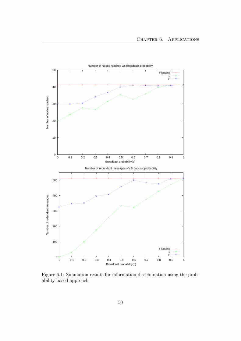
6.1.3 Experiments
In this section we present simulation results for the information dissemination
approaches discussed in the preceding section. We use the same system model
and setup as described in chapter 5-section 5.1. We analyze a sample highway
scenario(4km stretch with 2 lanes per direction), and 200 nodes are shown
below. All results are averaged over a randomly selected set of 20 (n/10)
nodes which initialized the broadcast at independent instances. Figure-6.1
shows the observed variations in the number of nodes reached and number
of redundant messages with p, for the probability based approach. Shown
in red, green and blue are the results for flooding, p-persistent broadcast
and congestion governed probabilistic broadcast respectively. We see that
although our approach increases the number of redundant messages over the
simple p-persistent broadcast, however, a considerable increase in the number
of nodes reached is also observed.
49
Chapter 6. Applications
0
10
20
30
40
50
0 0.1 0.2 0.3 0.4 0.5 0.6 0.7 0.8 0.9 1
Num
ber
of n
odes
rea
ched
Broadcast probability(p)
Number of Nodes reached v/s Broadcast probability
Floodingpp’
0
100
200
300
400
500
0 0.1 0.2 0.3 0.4 0.5 0.6 0.7 0.8 0.9 1
Num
ber
of r
edun
dant
mes
sage
s
Broadcast probability(p)
Number of redundant messages v/s Broadcast probability
Floodingpp’
Figure 6.1: Simulation results for information dissemination using the prob-ability based approach
50
Chapter 6. Applications
0
10
20
30
40
50
0 0.1 0.2 0.3 0.4 0.5 0.6 0.7 0.8 0.9 1
Num
ber
of n
odes
rea
ched
q
Number of nodes reached v/s q
FloodingDeterministic flooding with Broadcast threshold=0.5
250
300
350
400
450
500
550
0 0.1 0.2 0.3 0.4 0.5 0.6 0.7 0.8 0.9 1
Num
ber
of r
edun
dant
mes
sage
s
q
Number of redundant messages v/s q
FloodingDeterministic flooding with Broadcast threshold=0.5
Figure 6.2: Simulation results for information dissemination using the deter-ministic approach : Variation with q ;Broadcast threshold (bcastTH) is set to0.5
51
Chapter 6. Applications
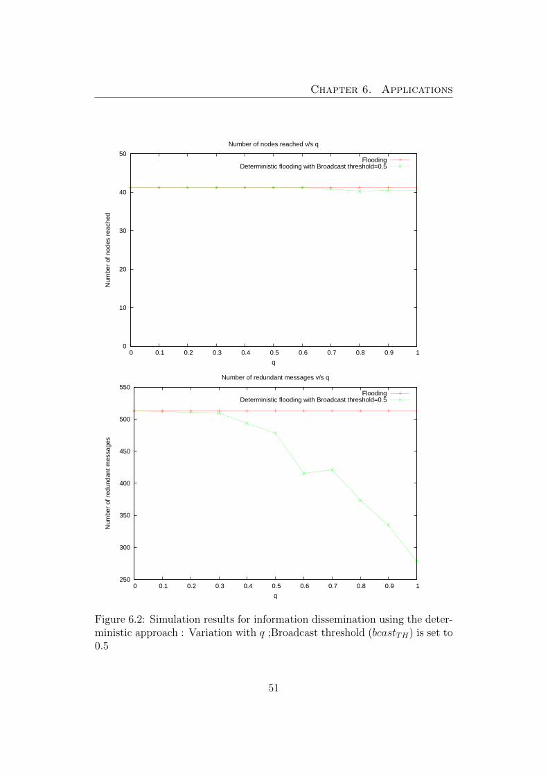
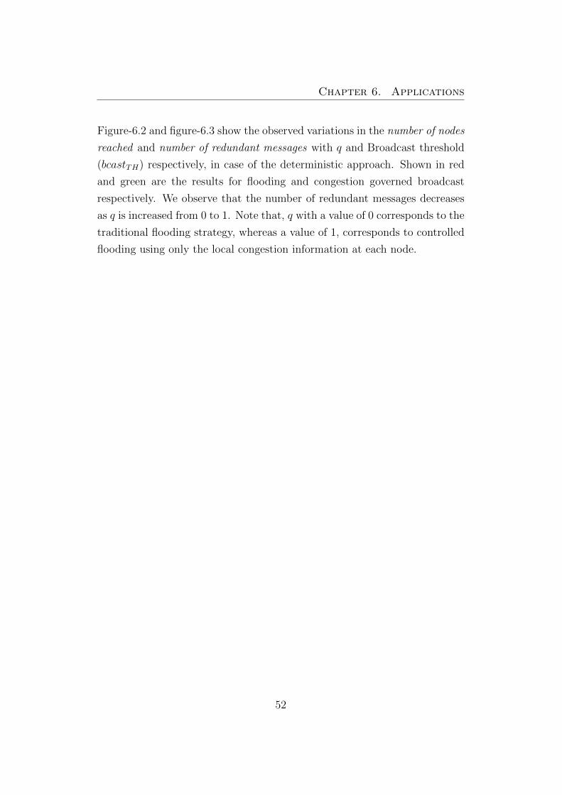
Figure-6.2 and figure-6.3 show the observed variations in the number of nodes
reached and number of redundant messages with q and Broadcast threshold
(bcastTH) respectively, in case of the deterministic approach. Shown in red
and green are the results for flooding and congestion governed broadcast
respectively. We observe that the number of redundant messages decreases
as q is increased from 0 to 1. Note that, q with a value of 0 corresponds to the
traditional flooding strategy, whereas a value of 1, corresponds to controlled
flooding using only the local congestion information at each node.
52

Chapter 6. Applications
0
10
20
30
40
50
0 0.1 0.2 0.3 0.4 0.5 0.6 0.7 0.8 0.9 1
Num
ber
of n
odes
rea
ched
Broadcast threshold
Number of nodes reached v/s Broadcast threshold
FloodingControlled flooding with p=0.5
0
100
200
300
400
500
600
0 0.1 0.2 0.3 0.4 0.5 0.6 0.7 0.8 0.9 1
Num
ber
of r
edun
dant
mes
sage
s
Broadcast Threshold
Number of redundant messages v/s Broadcast threshold
FloodingControlled Flooding with p=0.5
Figure 6.3: Simulation results for information dissemination using the deter-ministic approach : Variation with Broadcast threshold (bcastTH) ; Broad-cast probability (p) is set to 0.5
53
Chapter 7
Conclusion
This thesis demonstrated that how vehicular congestion estimation is aided
by means of VANETs and that it can be applied in many convenience and
safety applications targeted for VANETs. The preceding three chapters
have shown how the characteristic mobility pattern associated with nodes
in VANETs are a key factor in countering the extreme instability of links
between nodes in a VANET, as well as to establish the fact that congestion
estimation is an application which requires to differentiate between messages
of the same ‘type’ and hence differentiate their processing. The contributions
of this thesis have been threefold :
1. We assert that a need for characterizing messages according to the
‘importance’ or ‘relevance’ they bear for the application in question is
certain, as far as vehicular congestion estimation is concerned.
2. We have demonstrated how certain characteristics associated with spa-
tial mobility of a node coupled with the message transference over the
network may be used to measure quantitatively, vehicular congestion
surrounding a node.
3. We have shown how vehicular congestion surrounding a node can be
applied for dissemination of information, initialized from a single active
node, over the VANET.
54
Chapter 7. Conclusion
7.1 Future Work
Both convenience and safety applications over VANETs might benefit from
further research. Future work on vehicular congestion estimation might pro-
ceed along the following lines :
1. Although, an empirical calculation of the parameters involved is pre-
sented, the exact method of their determination in context of the
present surrounding traffic scenario of a node has been left un-specified.
Further work might investigate their correlation with other network and
mobility characteristics and a dynamic way to ‘learn’ them as the node
progresses through the traffic.
2. A more effective and efficient estimation technique could be developed
for estimation of global congestion of node. We suggest that exchange
of local congestion estimates to a reduced degree, by means of piggy-
backing may be employed to achieve the same.
3. The congestion estimation strategy can be treated as a lower layer, and
hence integrated with collaboration and misbehavior detection proto-
cols.
Further research into information dissemination over VANETs using vehicu-
lar congestion, might consider the following lines of inquiry :
1. While it has been established that a probability based approach using
vehicular congestion performs better in terms of the node coverage,
however, the redundancy increases as well. The exact nature of the
cause of this unseemingly feature needs to be investigated.
2. A deterministic approach using local information to infer the global in-
formation propagation pattern is shown potentially to be more effective
in propagation of information, however, on receipt of information at a
node, the local congestion can also be used in a ‘reverse-lookup’ way,
so as to determine the contribution that the sender would have had in
55

Chapter 7. Conclusion
propagating the information, and hence arrive at an adaptive decision
for broadcast accordingly.
56
Bibliography
[1] Haberman, R. 1977. Mathematical models: Mechanical vibra-
tions,population dynamics and traffic flow : An introduction to applied
mathematics .Engelwood Cliffs,N.J.,Prentice-Hall.
[2] M.Artimy, W.Robertson, and W.Philips, “Assignment of Dynamic
Transmission Range Based on Estimation of Vehicle Density”, in Pro-
ceedings of the 1st ACM International Workshop on Vehicular Ad Hoc
Networks[VANET], Philadelphia,Pennsylvania,Oct,2004.
[3] Kerner, Boris S. (December 2004). The Physics of Traffic: Empirical
Freeway Pattern Features, Engineering Applications, and Theory. Berlin:
Springer
[4] Fan Bai, Tamer ElBatt, Gavin Holland, Hariharan Krishnan, Varsha
Sadekar,“Towards Characterizing and classifying communication-based
Automotive Applications from a Wireless Networking Perspective”.
[5] M. Torrent-Moreno, P.Santi and H.Hartenstein, “Fair Sharing of Band-
width in VANET ”,in Proceedings of the 2nd ACM International Work-
shop on Vehicular Ad Hoc Networks (VANET), Cologne,Germany,
September 2005.
[6] “Car2Car Communication Consortium,” http://www.cat-to-car.org/.
[7] “Network Simulator ns-2”, http://www.isi.edu/nsnam/ns/.
[8] “VanetMobisim”, http://vanet.eurecom.fr/.
57
Bibliography
[9] Hall, F. L. “Traffic stream characteristics. In Traffic flow theory: A state
of the art report” - revised monograph on traffic flow theory, Oak Ridge,
Tennessee, Oak Ridge National Laboratory - 1997.
[10] D. Helbing, “Criticism of three-phase traffic theory”. Transportation
Research Part B: Methodische 43.
[11] Chen, Z. D., Kung, H. T. and Vlah, D. 2001. “Ad hoc relay wireless net-
works over moving vehicles on highways”, in Proceedings of the 2nd ACM
International Symposium on Mobile Ad Hoc Networking & Computing,
Long Beach, CA, USA.
[12] Kosch, T., Schwingenschlogl, C. and Li Ai. 2002. “Information dissem-
ination in multihop inter-vehicle networks”, in Proceedings of IEEE 5th
International Conference on Intelligent Transportation Systems.
[13] Rudack, M., Meincke, M., Jobmann, K. and Lott, M. 2003.“On traffic
dynamical aspects of inter vehicle communications (IVC)”, In Proceed-
ings of IEEE 58th Vehicular Technology Conference.
[14] Rudack, M., Meincke, M. and Lott, M. 2002.“On the dynamics of ad
hoc networks for inter vehicles communications (IVC)”. In Proceedings
of the 2002 International Conference on Wireless Networks. Las Vegas,
USA.
[15] Fubler, H., Mauve, M., Hartenstein, H., Vollmer, D. and Kasemann M.
“A comparison of routing strategies in vehicular ad-hoc networks” - 2002.
[16] Ghazy Ali and Ozkul Tarik, “Design and simulation of an artificially
intelligent VANET for solving traffic congestion”.
[17] Padron, Francisco M., “Traffic congestion detection using VANET ”.
[18] Wireless Access in Vehicular Environment (WAVE) in Standard 802.11
Information Technology Telecommunications and Information Exchange
Between Systems, Local and Metropolitan Area Networks, Specific Re-
quirements, Part 11: Wireless LAN Medium Access Control(MAC) and
Physical Layer(PHY) Specifications, IEEE 802.11p/D1.0, Feb. 2006.
58
Bibliography
[19] Vinu Rajshekhar, “An Integrated Traffic and Network Simulator for Re-
alistic VANET Simulation”, Bachelors thesis, IIT Kharagpur, May 2009.
[20] A. Vulimiri, A. Gupta, P. Roy, S. Muthaiah, and A. Kherani, “Applica-
tion of secondary information for misbehavior detection in VANET ”.
[21] T. Kosch, “Local Danger Warning Based on Vehicular Ad-hoc Networks:
Prototype and Simulation”.
59