trac pac 2 design and construction - connecticut · trac pac 2 teacher reference 1 design and...

TRAC PAC 2

Teacher Reference 1

DESIGN AND CONSTRUCTION

Building Only the Roads that We Need

ABSTRACT This module covers the educational topics of data visualization, goodness of fit, and law of sines covered in a high school geometry or mathematics course, management of technology to benefit society taught in a social studies course, and the positive and negative impacts of transportation systems along with computer algorithms discussed in a technology course. Transportation topics include horizontal curvature, traffic flow and capacity relationships used within traffic engineering, determining the “best” road location to acquire right of way, and traffic management systems. The first activity, How Much Traffic Can the Road Handle? is a 15-minute demonstration, illustrating how a roadway has a finite capacity: a maximum number of cars that can move through a lane within an hour. The popcorn portion (Parts A and C) is appropriate for middle and high school students, and the traffic flow portion (Part B) is appropriate for high school students. The second activity, Not In My Backyard!! is a one- to two-class-period, hands-on drawing exercise that asks students to determine how to align a road that will go from point A to point B, given that there is no optimal location for the road: students consider design consequences, costs, and environmental impacts. The third activity, How Much Does it Cost? uses spreadsheets and computer-based modeling to estimate real estate prices for the land that must be taken for the roadway. Activity 4, Keep Me on the Road! uses the High Roads computer aided design (CAD) software to create a road on the computer, given the challenge of incorporating horizontal and vertical curvature at different speeds. While Activity 2 (for middle and high school students) introduces the idea that a curve limits traffic speed, Activity 4, (for high school students) delves into the underlying mathematics.

Activity 5, Take the Short Way Home, is a computer programming exercise in Visual Basic for Applications (a language comparable to Visual Basic but included with Microsoft Excel), where students design a program to determine the fastest route between two points. Then, poor and good signal progression are compared with the Synchro/SimTraffic simulation package. This activity introduces the Intelligent Transportation System (ITS) concepts of sensors, traffic management systems, and software engineering. Teachers may elect to do all, some, or none of the five activities in this module. The five activities are suitable for groups of 2-4 students. Diversity within the group is recommended; e.g., for Activity 2, each group may want to include “an artist, an organizer, and a technical expert.”

TRAC PAC 2

Teacher Reference 2

DESIGN AND CONSTRUCTION

TEACHER REFERENCE

How to Use this Manual Quickly (including software installation) ..................................3 Possible Activity Answers

Activity 1 Evaluation Questions .......................................................................................8 Activity 2 Evaluation Questions .....................................................................................10 Activity 3 Evaluation Questions .....................................................................................13 Activity 4 Evaluation Questions .....................................................................................15 Activity 5 Evaluation Questions .....................................................................................19

Optional Enhancements for the Activities ........................................................................23 Quick Glossary ....................................................................................................................29

National Education Standards...........................................................................................30

ACTIVITY PAGES (suitable for teachers and students)

Activity 1: How Much Traffic Can the Road Handle? ..................................................31

Activity 2: Not in My Backyard!!..................................................................................43

Activity 3: How Much Does Land Cost?.......................................................................61 Activity 4: Keep Me on the Road!.................................................................................77

Activity 5: Take the Short Way Home ........................................................................107

VOLUNTEER’S PAGE..........................................................................................................137

TRAC PAC 2

Teacher Reference 3

HOW TO USE THIS MANUAL QUICKLY

Pick any one of the five activities. (See the activity table on the page that immediately follows each activity tab)

a c t iv i ty t a b le

T e a c h e r P r e p T im e I n C la s s T im e G r a d e /C o u r s e T e c h n o lo g y I n t e r n a t io n a l T e c h n o lo g y E d u c a t io n A s s o c ia t i o n S t a n d a r d s

activity tab

*Decide how many Activity Pages you want to hand to students. Either

Discuss with the class the pages of the activity preceding the Student Goal. Photocopy for the class only the pages from Student Goal to the activity’s end.

OR

Photocopy for the class the entire activity.

Tell students to read the earlier portions and begin work with the Student Goal.

Assign the evaluation questions you deem appropriate for homework or discussion. Questions are in the Activity Pages, and answers are in the Teacher Reference.

*The teacher reference is for the teacher only. The Activities pages are for students and teachers.

TRAC PAC 2

Teacher Reference 4

Installing Software From the Three CDs

Before starting, a teacher, student, or systems administrator should install the three CDs. This only needs to be done once per computer or per network. Although instructions will vary by platform (Macintosh, Windows NT, Windows 98), examples for each CD follow:

CD What Should Be Done With the CD? Construction CD Copy the entire Construction folder from the Construction CD onto

your hard drive (usually C:, D:, or E:). The free QuickTime movie player is available from www.apple.com/quicktime.

High Road CD Double click the file setup.exe or HighRoad.msi in the folder High Road Acad. 6.0.3 Installer to install High Road on the hard drive.

Graphical Analysis CD Follow instructions inside CD jacket to install Graphical Analysis onto the hard drive.

Example of Copying the Construction folder from the Construction CD to the Hard Drive

Double click on “My Computer”

Double click on the CD drive (R: in this example)

Single click on the construction folder and select Edit/Copy

Double click on the hard drive (C: in this example)

Select Edit/Paste to paste a folder called “Construction” to the hard drive.

TRAC PAC 2

Teacher Reference 5

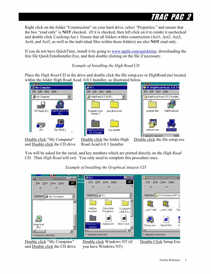
Right click on the folder “Construction” on your hard drive, select “Properties,” and ensure that the box “read only” is NOT checked. (If it is checked, then left click on it to render it unchecked and double click ConSetup.bat.) Ensure that all folders within construction (Act1, Act2, Act3, Act4, and Act5, as well as the individual files within those folders) are also NOT read only. If you do not have QuickTime, install it by going to www.apple.com/quicktime, downloading the free file QuickTimeInstaller.Exe, and then double clicking on the file if necessary.

Example of Installing the High Road CD Place the High Road CD in the drive and double click the file setup.exe or HighRoad.msi located within the folder High Road Acad. 6.0.3 Installer, as illustrated below.

Double click “My Computer” and Double click the CD drive

Double click the folder High Road Acad 6.0.3 Installer

Double click the file setup.exe

You will be asked for the serial, and key numbers which are printed directly on the High Road CD. Then High Road will exit. You only need to complete this procedure once.

Example of Installing the Graphical Anaysis CD

Double click “My Computer” and Double click the CD drive

Double click Windows NT (if you have Windows NT)

Double Click Setup.Exe

TRAC PAC 2

Teacher Reference 6

Possible Progression Through the Five Design and Construction Activities

The flowchart shown below is a guide, but any single activity can be selected at any time.

Pick an Actvity

Select “Activity Pages” to Give to Students

For a particular activity, giving students all the Activity Pages is advised if -- students have time to read the initial portion of the activity outside class, and -- class time is limited to only the interactive portions of the activity. Giving students only the Activity Pages from Student Goal to the activity’s end is advised if -- the teacher wants to reduce photocopying costs, and -- there is time to discuss the pages preceding the “student goal” in class.

Get Extra Help if Needed

If I want to Read Then Go To Page What software should be installed from the three CDs 4 Only how to do the activity itself!! 31, 43, 61, 77, or 107 Suggested answers for activity evaluation questions 8 Ideas for making the activity more challenging 23 Suggestions for the volunteer 137

TRAC PAC 2

Teacher Reference 7

Introduction to the Design and Construction Module

Transportation facilities -- urban freeways, sidewalks, bicycle lanes, traffic signals, rural two-lane roads, residential streets, and computerized traffic management systems that divert traffic during an incident -- require diverse skills to plan, design, construct, and maintain. These skills include problem solving, civil and systems engineering, economic analysis, communication, and an ability to make decisions given that no alternative is perfect. Activity 1 covers how a road’s capacity is affected by the design speed of the road, the size of the road, and the closeness with which vehicles can travel. Activity 1 is for the student who asks, “Why can’t everyone just drive faster in order to eliminate a traffic jam?” During the early 1900s, surface transportation in the U.S. focused heavily on roadways. Designers needed a strong grasp of mathematics (geometry, trigonometry, and algebra) to determine the maximum steepness for a road, whether a proposed horizontal curve was too sharp due to centrifugal force, or the road could accommodate stopping distances under poor weather. These geometric design skills matter today, as reflected in activities 2 and 4. Especially since the 1960s, the transportation planning process requires that roads not be built in a vacuum. Road builders may not lay a road through a community with impunity: instead, they have to consider the best way to minimize noise pollution, maintain water quality, and preserve existing development. These considerations are also part of Activity 2. Urbanization has made the acquisition of right of way for the road more important in the construction process. An important skill in Activity 3 is to model how land costs are influenced by the location of a piece of property as well as type of development (residential, commercial, or industrial). Modeling – determining the best type of mathematical equation that describes a set of data – is used in many other careers, such as investment banking or weather prediction.

Activity 5 dispels a common belief – that “transportation” only means building roads. Traffic management systems aim to move traffic more efficiently on existing roadways, using sensors (to collect traffic speeds and volumes), software routines (to determine where traffic may be diverted), and changeable message signs (to alert drivers to an impending traffic jam). Activity 5 lets students design and code a subroutine to select the faster of two routes. A simulation package then illustrates how coordinated traffic signal timing reduces the queue at a red light.

TRAC PAC 2

Teacher Reference 8

POSSIBLE ACTIVITY ANSWERS

Suggested Answers for Activity 1 Evaluation Questions These questions accompany Part C and may be done as a class discussion, especially Activity 4. A variety of answers are possible; answers below are given using the example shown in Table 7. 1. Compare the average flow rates for the smaller funnels and the larger funnels.

average flow rate for the larger funnel = 100 ml/sec average flow rate for the smaller funnel = 23.5 ml/sec The smaller funnel has a flow rate that is 77 % less than the larger funnel

since (23.5 - 100)/100 = 0.765 ≈ 77% 2. Compare the areas of the funnels. diameter of the larger funnel = 1.3 cm diameter of the smaller funnel = 2.3 cm area of the larger funnel = π(radius)2 = 4.15 cm2 since 3.14(2.30)2 ≈ 4.15 area of the smaller funnel = π(radius)2 = 1.33 cm2 since 3.14(0.65)2 ≈ 1.33 The smaller funnel has an area that is 68 % less than the larger funnel since (1.33 - 4.15)/4.15 = 0.6795 ≈ 68% 3. Is the percentage computed in Question 1 the same as the percentage computed in

Question 2? ______yes ______no This is the student’s call. The teacher may suggest that being within 10 percentage points

should be considered “the same.” 4. Suppose that the kernels represent drivers, the funnels represent the width of the

roadway, and the smaller funnel represents a work zone or accident that temporarily closes part of the road.

What does your answer in Question 3 suggest about the effect of a lane closure?

TRAC PAC 2

Teacher Reference 9

If the answer is yes, then this means that the effect of closing a lane has a proportional impact on flow rates: if one decreases a road width from two lanes to one lane, for example, then one will decrease the amount of traffic flow by 50%.

If the answer is no, then this means that the effect of closing a lane has a disproportionate

effect on flow rates. For example, using the computations above, a 68% decrease in capacity caused a 77% decrease in traffic flow.

In practice, it is often the case that a small decrease in roadway capacity has a large

decrease in traffic flow. For example, it has been suggested that in some instances, closing one lane of a three lane highway will decrease capacity by more than 33%. In periods of heavy congestion, even a small obstruction on the shoulder – such as a disabled vehicle – can greatly decrease the traffic flow on a roadway. One can also criticize the popcorn analogy in the sense the drivers are not like popcorn kernels: they will have different reactions in times of traffic turbulence.

TRAC PAC 2

Teacher Reference 10

Suggested Answers for Activity 2 Evaluation Questions 1. Were you able to meet all of your original criteria in the steps 1-4 or did you have to

change your answers to steps 1-4: (a) My road met all of my original criteria in steps 1-4 (b) I had to change my criteria in Step 1, 2, 3, or 4 to build the road Probably most students will answer (b). That is fine; it emphasizes the point that the

perfect solution does not exist. 2. Determine the total cost of the road by adding the costs of the individual cells. This

can be done by hand or it can be done with the spreadsheet software. The cost is $_______ in millions This will vary by road, but remind students to simply use the data in Table 6. The value of doing this comes from comparing answers amongst students in the class and pointing out that students who did two-lane roads (with low design speeds) will generally have lower costs than students who chose six-lane freeways with high design speeds.

3. Determine the environmental impacts by counting the cells inside any buffered areas

from step 3 (such as the Snake River). A total of ________cells are affected by runoff or noise pollution. The answer will vary for each student. The lesson is that a road can affect an area even if

the road does not physically touch the location. 4. Indicate the number of homes and businesses that will have to be relocated by the

road _______homes will have to be relocated

_______businesses will have to be relocated In this simplified manner, we are counting each dwelling unit (regardless of size) equally and each business (regardless of size) equally. This simplifies matters but in reality is a bit unrealistic.

5. What percentage of the time will your road have enough capacity to avoid a traffic

jam (e.g. breakdown conditions)? (See Tables 2 and 8). Students simply compare the capacity of their road from Table 2 to the percentage of

hours shown in Table 8, where the capacity exceeds the volume. For example, suppose a

TRAC PAC 2


student chose the four-lane arterial with a design speed of 50 mph. See the following comparison in Table 8:

Table 8: Hourly Demand for the Road

Hours of the Day Volume of drivers who would like to use the road

Capacity of the Four Lane 50 mph Arterial

Is capacity sufficient?

7:00 - 8:00 am 10,000 6,400 No 10:00-11:00 am 6,000 6,400 Yes 1:00 - 2:00 pm 3,000 6,400 Yes 4:00 - 5:00 pm 9,000 6,400 No 6:00 - 7:00 pm 12,000 6,400 No For this particular road, there will be sufficient capacity about 40% of the time. During

the remaining 60% of the time, there will be breakdown conditions. (Engineers refer to these breakdown conditions as “level of service F”).

6. Indicate which goal is best achieved by your road (Tables 3 and 4 may be helpful). (a) move a lot of traffic (b) minimize environmental impacts such as water runoff and noise (c) consume as little land as possible (d) increase pedestrian safety (e) encourage economic development in rural areas.

This will relate to the chosen road and there may be more than one correct answer. For a high speed freeway, the answer should be (a). For a two-lane low speed roadway, the answer may be (c). A road’s location may also influence which of these is chosen; a road connecting rural areas could qualify for answer (e).

7. Indicate which of the following constituents is likely to be the most content with the

construction of the road. (Table 5 may be helpful).

(a) residents of ____________________________________(name the areas)

(b) through travelers that do not live in the community (c) small business owners (__________________________name a few that apply) (d) The Western Forest Preserve Conservation Society (e) the Airport Authority Encourage students to discuss which of these constituencies would also be unhappy with

the decision. For example, if the road goes to the east (far away from the forest preserve) then the Western Forest Preserve Conservation Society in answer (d) will be happy, however, the Airport Authority in answer (e) will be disappointed if a large road does not serve the airport.

TRAC PAC 2


8. What can you conclude is the “best” decision for this community if they decide they want a new road?

This activity should convey that there is no single decision that will please everyone. Instead, a community has to consider the different goals it may have and the different constituencies, and draw some sort of compromise amongst these. (It is true that there can be cases where a new road may satisfy all goals, but often some type of compromise is necessary).

9. The location for a road that is guaranteed to make all citizens happy is probably

(a) in a rural area (to encourage economic development) (b) in an urban area (so as to preserve farmland) (c) in the mountains (to provide a scenic view) (d) within driving distance of major residential neighborhoods (e) probably no location will please everyone! Should be (e) although students may come up with some excellent ideas that justify another answer: if so, then accept their answer!

10. What mode of transportation was not fully considered in this example (but should

be considered in real life)? (a) bicycle (b) walking (c) public transportation (buses) (d) public transportation (light rail or “subways”) (e) all of the above (e) This activity leaves out a critical lesson: that transportation should truly be multimodal in focus. An extension of this activity would be to discuss how a combination of transportation options, such as high speed rail where there is heavy demand or paratransit for those who need reliable transportation service but do not have access to a vehicle, would be a better solution than simply building a new road.

TRAC PAC 2


Suggested Answers for Activity 3 Evaluation Questions 1. Suppose one is comparing different models and one produces a graph of true prices

versus predicted prices as shown in Figure 12a above. How will the graph for a more accurate model compare to the graph for a less accurate model?

As a model increases in accuracy, the predicted values (e.g. MyPrice) will be closer to the actual values (e.g. TruePrice). Thus the graph for a more accurate model would be more similar to a 45 degree line (e.g. what is shown in Figure 13b).

*2. For the Mega Mall of America, the total cost is given by summing the costs for cells

G7..J10. What is the total cost that your model predicts?

Assuming students used the formula Cost = 30,000/Distance2, the predicted costs for the 16 cells (G7, G8, G9, G10, H7, H8, H9, H10, I7, I8, I9, I10, J7, J8, J9, J10) would be around $22,300. Of course, the students may use a different formula.

3. Suppose that Mega Mall actually sells for $20,000. How accurate is your model?

The actual cost is $20,000__

The predicted cost is $22,300 (or whatever answer students have)

The difference is $2,300

The percent error is the difference divided by the actual cost and multiplied by 100.

The percent error is 11.5% 4. Suppose a real estate agent wants a model that can predict costs within 25% of their

actual value. Based on the performance with the MegaMall of America, is your model accurate enough?

___yes ___no

The answer is “yes” for a model of Cost = 30,000/Distance2

TRAC PAC 2


5. Using the Mega Mall as an example, why might a model that predicts cost as even be of value? Why not just ask the owners of Mega Mall directly?

If we wanted to estimate land prices but could not quickly determine the real prices, then a model can be a quick way to make a guess. No model can ever replace real world data, but there are some situations where a model can help us make a guess when we are missing information.

*6. What is the value of the MegaMart shown in cells X10..Z11 using the above formula?

Based on the formula 2

50,000one cell of commercial land = distance from the road

the answer should be close to $300,000. *7. What would be the value of MegaMart if it were located 5 units from the road rather

than just 1 unit?

The answer should be close to $12,000. 8. If this model were accurate, then what effect can transportation proposals have on real

estate prices?

It can occur that plans to build a nearby road can cause an increase in land prices. However, it should also be pointed out that road plans can cause prices to decrease, depending on the type of development that is near where the road is located. It is also argued, by some, that roads do not encourage new development but rather influence the location where this new development would occur. Overall, it should be pointed out that spreadsheet modeling such as this gives one a tool with which to make some forecasts in the absence of better information, such as what potential sellers are really willing to accept in return for selling their land.

In the above example, it can be discussed that the location of the road greatly influenced MegaMart’s land value! Imagine if MegaMart were fixed in location but the road was not yet built: if the model were accurate, then one could see the owners of that land being very interested in having a road that was close by, if it could raise the value from $12,000 to $300,000.

TRAC PAC 2


Suggested Answers for Activity 4 Evaluation Questions

1. Roadway sections are often referred to as either a “cut” or a “fill” section. Why do you think that engineers refer to the section of road shown in Figure 24(b) as a cut section?

Cut sections require that earth be removed in order to lay the road (e.g. a road carving through a mountain would likely be a cut section) whereas fill sections require that earth be added in order to lay the road.

2. Find the chainage for a fill section (e.g. between 0 and 1000). There are many possible answers. A fill section will be one similar to that shown near

chainage 380 (e.g. the figure below), where the road is elevated above the sides.

3. Look at the plan view on your screen (similar to the left side of Figure 27). As a

motorist rounds the vertex of the main horizontal curve near chainage 300, will she be going up a hill or going down a hill? How can you tell?

One can move the marker shown in the profile view from 260 to 340. As one does this, one

sees to the left (the plan view) that the marker is rounding the curve, and one sees to the upper right (the profile view) that the marker is going down a hill until approximately chainage 280, at which point it starts going up a hill. Answers will vary depending on how the student has constructed his or her individual road: the important element is that students see how the plan and profile views relate.

4. Given the existence of natural and man made features, what are some general reasons

for why there might be a horizontal curve such as that shown in Figure 27? There are at least two main possibilities, although these may or may not apply to the situation

shown in Figure 27.

· A horizontal curve may reduce cut and fill costs if the horizontal curve can keep the road on the same plane (e.g. level). The contours themselves in Figure 27 do not necessarily support this, but one can envision a situation where one keeps the road on the same contour, where the contour is not a straight line but rather has horizontal curves as shown in Figure 27.

TRAC PAC 2


· A horizontal curve may bypass man made or natural features, such as lakes, rivers, houses, and businesses. For example, the lake shown in Figure 27 is bypassed by the existing road.

5. What color does the entire road become? The entire road should change from red and yellow to yellow only. 6. What happens to the horizontal curve? The sharp horizontal curve near chainage 300 should disappear: now the road is mostly a

straight section. 7. Why do you think the color changed? The color red reflected a too-steep curve, one where the radius of curvature (R) was too small

given the design speed of 60 km/h. Thus the curve was unsafe, and by eliminating the curve the hazard was eliminated, changing the road section to yellow.

8. Given the design speed of 120 km/h, how can you fix your horizontal alignment in order

to eliminate the hazardous (red) sections? Are there any disadvantages to your solution?

The answer is to align all of the horizontal intersection points as shown in the figure below.

This way all of the curves are eliminated. However, two potential problems may result: one has a lot of expense because of the boundaries that must be traversed (mountains and valleys shown by the contours, the lake which will require a bridge, and so forth) and one has environmental consequences (runoff from the road may affect the water in the lake and one may have to destroy homes and businesses that would have been preserved had the road had the horizontal curve within it).

TRAC PAC 2


9. Using the equation to compute the minimum radius of horizontal curvature, what

minimum value of R is necessary in order to accommodate the design speed of 60 km/h given the values of Fs and e shown immediately above?

( ) ( )

2 260 123 m127 127 0.16 0.07s

vRF e

= = =+ +

10. Is your actual radius of curvature (shown in Figure 29 as 84.30) larger than the

computed radius of curvature in question (9)? _____yes X no No: 84.3 m (the actual radius of curvature) is less than what is needed (123 m) 11. Suppose all horizontal intersection points are fixed except the third intersection point.

Write down the actual value of R (shown in Figure 29 as 84.30) but your value may be different.

84.30 (but almost any value is acceptable)

TRAC PAC 2


Then close the transitions window. Now move this intersection point very slightly to the left. Reopen the transitions window (Window/Transitions). Write down now this new value of R.

an example is 90.04 (this number should be greater than the underlined number above)

What happened to the actual value of R as you moved slightly to the left?

R should gradually increase: what this means is that you are increasing your actual radius of

curvature or decreasing the sharpness of your curve. 12. Suppose you start moving the horizontal intersection point very slowly to the left.

Using only the value of R shown in your transition view (e.g. what you have in lieu of the “84.30” in Figure 29), can you predict when the roadway section will change from red to yellow?

As the point is moved to the left, the road becomes straighter, and the radius of curvature R

increases. The road will change from red to yellow once the minimum radius of curvature (e.g. 123 m) is surpassed. The figure below shows an R value of 128.04 m which means the curve is gradual enough to meet the minimum standard of risk.

TRAC PAC 2


Suggested Answers for Activity 5 Evaluation Questions For questions (1) – (3), consider this line of code.

LeftCarF(K).Top = LeftCarF(K).Top - StepSize + Int((StepSize * 0.5 * Rnd) + 1) * (-1) ^ (Int(10 * Rnd)) 1 What happens to the oscillations of the following left cars if you change 0.5 to 0.01? The oscillations decrease down to almost nothing. 2. What happens to the oscillations of the following left cars if you change 0.5 to 2.0? The oscillations increase dramatically; the following left cars seem to “jump around”

quite a bit. 3. Thus what is the role of the underlined 0.5 in terms of the random component of the

following distance? The 0.5 acts like a weighting factor for the random component. The following distance is

determined from two components: (a) the speed and (b) a random component. Thus increasing the 0.5 to a larger number makes the “randomness” more important—the oscillations will increase quite a bit and become the main determinant of the distance between the lead car and the following cars. Decreasing the 0.5 to zero, on the other hand, eliminates the randomness completely. Time permitting, the instructor may wish to discuss other techniques for generating random numbers within a specified range and why those techniques can be useful when doing simulations.

For questions (4) - (6), assume that the user interface done in step (2) has been completed. 6. Compare your answers for questions (4) and (5). Why might your answers suggest

that a critical early step in designing software is to understand exactly what the user wants done?

Answers for questions 4 and 5 will vary; there are no wrong answers. If students indicate

that the animation (question 5) is more work than the computations (question 4) then it should be clear that not all tasks users want done require the same level of effort. Thus, before embarking on a difficult task (such as developing the animation for question (5) above), it is good to ensure that the user, or client, has indicated exactly what they want.

For questions (7) – (9), suppose the application you just developed could accurate predict traffic speeds on two parallel routes. Suppose also you know that in the next hour, 200 vehicles are planning to use the minor road and 5800 vehicles are planning to use the freeway. 7. Without any route diversion, what will be the average speeds on the freeway and the

minor road?

TRAC PAC 2


56 mph on the minor road 13 mph on the freeway _______mph overall The “56” and the “13” come directly from the software. Overall, one has 56 mph (200 vehicles) + 13 mph (5800 vehicles) = 14.43 mph 8. Suppose you have a network of changeable message signs on both routes such that

you can divert traffic from the freeway to the minor road (or vice versa). Would you put a message on the changeable message sign telling drivers to divert?

X yes ____no [Answers may vary!!] Students may not agree on how many cars to divert, but hopefully they will see that given

the large number of very slow cars on the freeway, some improvement can be made by using some of the excess “space” or capacity on the two-lane road.

9. Suppose you answer “yes” and that you have sensors that indicate exactly how

many drivers heed your instructions. How many drivers would you keep on the freeway and how many would be on the minor road if you wanted them to have equal speeds?

4500 freeway cars + 1500 minor road cars = 6,000 cars total at speeds of 28 mph

Remember that questions (10) – (12) are probably more suitable for a class discussion than for individual written answers. These answers are also a source of activity enhancements. 10. Is your diversion (in question 9) better than doing nothing (in question 7)?

A point for discussion is that there are a lot of possible techniques for considering what is a “best” diversion. One technique -- implied in question (9) above -- is to divert traffic until speeds are equal, although it should be pointed out that not everyone will necessarily be equally happy about this. Another option would be to divert if speeds drop below a certain threshold -- e.g. one might say that for freeways, speeds below 40 mph require diversion but for the minor road one does not divert until speeds are below 20 mph. Students with a stronger math interest may wish to discuss how speeds are actually computed. The equation for computing freeway speeds, e.g.

802300 ( )

Freeway VolumeFreeway SpeedNumber of Lanes

=

is only an approximation that assumes a linear relationship between volume and speeds. In practice, however, it has often been the case that freeway speeds are relatively constant from zero to a moderate volume per lane, and then as the volume increases further (say to 1,800 cars per lane) then the speeds start to drop dramatically. However, this relationship

TRAC PAC 2


depends on the percentage of heavy trucks, the grade, the lane and shoulder width, and the driver population. If a volunteer is present, the volunteer can discuss practical impediments to making route diversion work, such as (a) getting accurate data in the first place in spite of imperfect sensors, software failures, and limitations on where sensors can be placed, (b) having changeable message signs or radio messages that drivers understand, (c) drivers heeding or not heeding the messages, (d) staffing a TMS with enough people to assist with diversion, and (e) finding alternative routes that are not as congested as the main route that can be used by diverted traffic!

11. An unusual feature of this activity is that you designed the application yourself.

Realistically, however, a large scale software project would be done in groups, with one team of persons designing the user interface, one team of persons designing the logic underlying the program, one team of persons testing the software, and so on. If you were designing this software in large teams, what considerations would you need to make in order to work together effectively?

Three big items that should be resolved are

(a) the overall design of the software, as in how the individual pieces will fit together (b) who will be responsible for which piece (c) common variable and file names. A simple but critical example of (c) is that if the person doing the user interface decides on a particular name for an object (e.g. “LeftCar”) than the person designing the logic needs to use that same name. In practice, one can often develop common naming conventions, along with well documented variables, to make working together easier. Another example is with the worksheet naming: if one calls “sheet1” something else, then the code that refers to “sheet1” will produce an error! The names used in the coding and the names used with the worksheet need to be consistent.

12. Take another look at how the program was written. Given that the computations in step (3) already indicate the speed as a function of the traffic volume, for what reasons might one use the animations shown in step (4)?

There are a couple of reasons.

· First, one might wish to convince decision makers about a particular alternative -- for example, one might say that “if too much traffic is on the freeway, speeds will drop to 20 mph instead of moving along at 50 mph”--but the message can be much more convincing if one can show animations or photographs of what is occurring. With these animations, one can show motorists real time traffic conditions over the Web OR one could convey to an audience a better understanding of the benefits of investing in technologies that will enable route diversion during periods of heavy congestion.

· Second one might be able to better understand what is happening on the road under certain conditions. For example, suppose a more complex animation where (as

TRAC PAC 2


happens in the real world upon occasion) “stop and go traffic” was shown, where average speeds suddenly increased and decreased. With short following distances, one might better understand how rear end collisions were occurring, and what could be done to prevent them.

Teachers who have extra time or who have students who wish to explore this further could consider making the following modifications to the activity. · Insert different pictures that hotrod.bmp or VBCar.wmf. The statement

LoadPicture(ActiveWorkbook.Path + "\VBCar.wmf") looks for a picture (VBCar.wmf) in the same folder as the active workbook (ConstructionActivity5.xls).

· Add a random following component for the freeway cars, and make the freeway cars’ position vary within each lane.

· Give the user a text box or list box control so that they can control the amount of random variation. Users could be asked to indicate what percentage of the following distance is controlled by random variations as opposed to speeds.

· Use different methods for computing speeds. For example, one can modify the equations shown previously such that the one multiplies the “60” in the minor road speed computation by a term that reads (1-volume/2800)X where x is an integer exponent between 1 and 5.

· Expand the scope of the animations to include different roadway types as well as different average speeds within the same roadway type (e.g. simulate vehicles slowing down for a curve).

· Explain how debugging works in general. Note that you can “debug” your program (e.g. determine the value of any variable) by inserting a line of code such as “[A1] = LeftCarF(1).Top”. This code will place the value of the LeftCarF(1).Top in the cell “A1”. This technique is useful when one has a long program that is producing an error, yet it is not immediately obvious where the error is occurring. By writing statements (such as the italicized one above), one can check the values of key variables as the program runs and eventually determine why the program is giving a different output from what was expected.

TRAC PAC 2


OPTIONAL ENHANCEMENTS Teachers who have already completed the activities shown in the Activity Pages may wish to extend, or enhance, these activities further. These enhancements are optional and should not be undertaken until the teacher has reviewed the Activity Pages.

· using the Web to create a map for activities 2 and 3 · doing activity 2 as an open-ended exercise · evaluating additional transportation/land use options for activity 3 · creating different movies for activity 4

Using the Web to Create a Map as An Alternative for Activities 2 and 3

The map that accompanies this module is designed for activities 2 and 3 and presents the layout of a hypothetical city. If teachers so choose, of course, another map may be substituted for this map. Whether using this map or a substituted map, five caveats should be kept in mind:

· The purpose of the map is to convey some of the obstacles to laying out a roadway and to enable students to make tradeoffs for what must be taken.

· The map should be large enough so that students can have a bird’s eye view of the entire

community. For the map that accompanies the module, it is comprised of two 11” by 17” inch sheets of paper that can be taped together.

· For ease of reference, the map is divided into rows (1-38) and columns (A-Z) such that

students may reference any location by giving the appropriate row and column. · Rows 1-19 correspond to the top sheet and rows 20-38 correspond to the bottom sheet. · The map does not have to be drawn to scale but it should enable one to understand some

of the challenges that are faced when deciding where a road should be placed.

One exhaustive website for maps is http://maps.langenberg.com. It includes about twenty different map searches. In the City & Highway area of the site, the best choice is ESRI, a GIS site. It will return a map for any city entered in the field. A suitable view can be found by zooming in and out and scrolling around city. The benefits of using maps from this site is that is shows the locations of schools, hospitals, and parks which makes area identification easier, as shown in Figures 1a and 1b.

TRAC PAC 2


Figure 1a: Map of Charlottesville, VA from Figure 1b: Map of Charlottesville, VA from ESRI on maps.langenberg.com Topozone.com

If the exact street address of a location that is to be used for this project is known, then a good map site is http://maps.yahoo.com. The address can be entered in the field, and this website will return a map with that address in the center of the map. This site only shows street names. Since both these sites return maps that already show street locations and names, then the project can include road widening exercises, or creating a new road through open areas. The drawback with these maps lies in the degree of detail. The ESRI maps only show schools, hospitals, cemeteries, and landmarks, but do not show all buildings. The Yahoo maps do not show any buildings. So it is impossible from information on the map to distinguish between areas that are heavily developed and areas that are open where it would be easiest to build a road. If students knew the area that the map depicted, they might be able to make the distinction from personal knowledge, but they still would not know the exact location of buildings from the map alone. Another option is using a topographical map from www.topozone.com. This map accurately shows most buildings in an area, but the only drawback is that many of these maps are out of date. In cities, the map simply displays heavily developed areas as pink. In areas that are less developed, the individual buildings are represented by black boxes. The color green depicts forests and thick vegetation. An example is given in Figure 1b. The last possibility, but least consistent in returning correct maps, is the Satellite Photographs option on www.maps.langeberg.com. A city and state must be entered in the field, and then the server reroutes to a MSN site, as shown in Figure 2. Depending on the city, it might return a satellite photograph, aerial photograph, or just another topographic map. It lists options for each city, and for some cities there might be options ranging from satellite photographs to topographic maps, and for other cities the only option will be a topographic map. If a satellite or aerial photograph is returned, use the large map option and zoom around the city to find the optimal location. Nothing is written on these maps, they are simply composites of aerial or satellite photographs. It might be difficult to determine exact locations, but a topographical map with place names is provided on the side of the web page to show where the photograph is centered.

TRAC PAC 2


Figure 2: Aerial Photograph of Winston-Salem, NC from Satellite Photographs on maps.langenberg.com

In short, regardless of the option that is chosen, the teacher should aim for a map that students would find familiar. It could be saved to the hard drive and printed out so a transparency grid could be placed on top. Some of the maps like the Yahoo map can be copied directly from the Internet and pasted into a program like Adobe or MSPaint. The aerial and satellite maps are divided up into small sections, so the best way to capture those to use in this project would be to use the print screen function and paste it in Adobe. From there, the toolbars could be cropped and students could use the map as a whole image. Copies may be printed out for each student that would show the map with the grid overlay similar to what is provided in Construction Activities 2 and 3. All three of these maps are free and easy to access. In short, students can choose an area near their house or an area where they think a new road needs to be added or an existing road needs to be widened.

Doing Activity 2 as an Open-Ended Exercise Although some teachers may prefer this as a structured activity, it is also possible to use these maps (or other maps) in order to perform this activity as an open-ended exercise. The basic steps of the activity can be modified, for example, to the following: 1. Discuss the different types of land uses and different types of roads that are possible. 2. Discuss potential conflicting goals (e.g. economic development, rural preservation) 3. Draw three proposed alignments for the roadway on the map lightly in pencil. Draw the

turns very lightly. 4. Consider what type of road is appropriate: two lane winding road, four lane arterial with

sidewalks and signals, or six lane freeway. 5. Determine the turns required for each roadway type, modifying steps 3 and 4 if necessary.

TRAC PAC 2


6. Draw a border around the proposed alignments to simulate noise and runoff impacts, where the distance from the border to the road is proportional to the size of the road.

7. Determine who would be satisfied/dissatisfied by each alignment. 8. Pick the “best” alignment and determine the cost of the land required for right of way. Students would then answer five open ended questions after designing their ideal road: 1. What are the environmental impacts of your road in terms of noise and water runoff? 2. How does the cost of your road compare with the cost of other alternatives? 3. How effectively does your road move a large amount of traffic compared to alternatives? 4. What constituents are likely to be the most pleased with your decision? 5. Which constituents would most likely object to your decision?

Adding Transportation/Land Use Interactions to Activity 3 After activity 3 has been completed, students can use data set 4 in the file constru3.dat (in Graphical Analysis) or the sheet extra in constructionactivity3.xls (in Microsoft Excel) to do the following, if they have already done activity 2:

· Compare the costs of the high speed freeway and the low speed arterial that were

considered in activity 2. Thus students would place a “1” in the cells for each layout and compute the totals. Although the results may not be surprising in that the more narrow road costs less, they are interesting to discuss in that the more narrow road costs significantly less than the larger road.

· Compute the amount of land (and thus cost) required for a high-speed curve as opposed

to a low-speed curve. Using the curve tools, select an area that a road has to bypass, such as the forest of gloom. One should observe that the 113 km/h (70 mph) curve tool requires a much greater arc than a 48 km/h (30 mph) curve tool.

· (for advanced computer science students). Develop a land use/transportation model.

Advanced students may wish to consider the following scenario if Excel is available (or a comparable spreadsheet). Use the map sheet in the file constructionactivity3.xls and identify each vacant area (marked with a “v”) as well as each commercial area (marked with a “c”). Replace each “v” cell with the formula “0 + amount” and each “c” cell with the formula “5 + amount”. Then, copy the entire map from cells a1..aa39 to a new sheet. Establish a reference value for “amount” as 0. Then, write a Visual Basic macro that does the following:

--copies the entire map to another place within the same sheet --increments the values of the vacant cells by the following formula

new vacant cell value = current vacant cell value + .1(sum of all adjacent cells/8)

TRAC PAC 2


Then, write a Visual Basic macro that converts each cell to a “c” if it is above a value of 5. By iteratively doing this procedure, one can see a map of land use development change over time.

Technical Tip: Creating New Data Sets in Graphical Analysis In Graphical Analysis one can create smaller data sets as follows

Step 1: Sort the data by some variable. (In this example, we sort the data by landuse, by going to Data/Sort and choosing the variable landuse as shown in Figure 3 below.

Figure 3: Sorting the Cells by Land Use in Graphical Analysis

Step 2: use the mouse to select all rows with landuse = 4 Step 3: Select Data/New Data Set Step 4: Scroll to the right to get to Data Set 3 Step 5: Selecting Edit/Paste, such that data set 3 now has only the cells with landuse =4.

Hint: If the mouse causes the rows to scroll too fast, then the shift key will reserve your place. When you get close to the border between landuse 4 and landuse 5, hold the shift key down and use the arrow keys to increment until you have highlighted all cells with landuse = 4.

Creating Different Movies for Activity 4 The creation of movies (animations) in the roadway design activity (activity 4) only scratches the surface in terms of (a) the basics of geometric design and (b) the capabilities of roadway design software. Without probing the software further, teachers with the assistance of a volunteer can discuss the impact of vertical curvature on highway safety as well as the role of public outreach when a community is considering possible designs for a roadway improvement or new

TRAC PAC 2


construction. For teachers who wish to explore more of the software’s capabilities, additional work can be done with computing the amount of earth that must be cut or filled (with this design) or viewing alternative designs (e.g. different typical sections). If a volunteer is available, that volunteer may have access to other digital terrain models for specific locations within the state or even closer to your school. Finally, if students have an interest in drawing or graphics, one can experiment with the views provided by different roadway designs such as that shown in Figure 4.

Figure 4: Alternative Roadway Design for Activity 4

TRAC PAC 2


QUICK GLOSSARY

animation: A movie that is produced with the assistance of three dimensional visualization software or design software. (Activity 4)

capacity: the maximum number of vehicles that a road can accommodate in an hour.

Capacity for a freeway is just under 2,400 vehicles per hour for each freeway lane under ideal conditions, such as flat terrain, no trucks, drivers who know the area, good weather, and daylight travel. (Activity 1,2,5)

density: the number of vehicles per kilometer or per mile. (Activity 1) design speed: the speed at which motorists may drive safely on a road. (Activity 4) flow rate: the number of vehicles passing a point within a specified unit of time. For

example, the flow rate of a freeway may be as high as 600 vehicles per lane over a 15 minute period. (Activity 1)

land use: The manner in which land is developed: examples include residential

only, commercial only, agriculture, and mixed use, such as homes interspersed with restaurants. (Activity 2,3)

radius of curvature: the sharpness of a roadway curve. A larger radius can accommodate

higher speeds; a smaller radius requries vehicles to slow down lest they run off the road due to centripetal acceleration. The radius of curvature is also called the turning radius. (Activity 4)

spacing: inter-vehicle spacing refers to the distance between vehicles on the road.

A similar term, headway, is the distance between the front bumper of one vehicle and the front bumper of the following vehicle. (Activity 1)

speed: the amount of distance that can be covered by a vehicle over a set amount

of time. For example, uncongested freeway speeds might be as high as 113 km/h or 70 mph. (Activity 1,2)

tangent sections: the two straight segments of road that need to connected with a smooth

curve. (Activity 4) TMS: Traffic Management Systems, which obtain use roadway speed and

volume data to alert motorists of delays and alternate routes. (Activity 5) VBA: Acronym for Visual Basic for Applications, a programming language

similar to Visual Basic but designed expressly for Microsoft Excel. (Activity 5)

TRAC PAC 2


NATIONAL EDUCATION STANDARDS

Activity 1: How Much Traffic Can the Road Handle? National Council of Teachers of Mathematics Standards. The algebra standard indicates students should use “mathematical models…including graphs, tables and equations”. Activity 1 has students create and interpret their own graphs from equations that predict traffic speed as a function of the number of cars. International Technology Education Association Standards. The focus of activity 1 is the theme “Transportation Technologies: Transportation Processes and Efficiency”. Standard M, “The Designed World” notes “determine capacity of lanes, traffic flow, and potential congestion problems”, computations that are done in this activity. Activity 2: Not in My Backyard! National Council for the Social Studies Standards. Strand 8 Science, Technology, and Society: (relationships among science, technology, and society) asks “How can we manage technology so that the greatest number of people benefit from it?” Activity 2 considers the technology to be a new road and asks how that road should be designed, what speed limit should be set, and where it should be placed, given the views of different constituents. International Technology Education Association Standards. Activity 2 focuses on the theme “ Positive and negative impacts of transportation systems”, including congestion and environmental impacts [shown in activity 2 as congestion delays, displacement of homes and businesses, noise pollution, and water quality.] Activity 3: How Much Does it Cost? National Council of Teachers of Mathematics Standards. The Data Analysis and Probability Standard indicates that students should “understand scatterplots and use them to display data … conduct analyses of the relationships between two sets of measurement data ...produce lines that fit the data ….[and] discuss what best fit might mean” Activity 3 focuses on these goodness of fit measures, and while students are not expected to define a residual or an R square value, they see a graphical representation of how they want to minimize residuals. Activity 4: Keep Me on the Road! National Council of Teachers of Mathematic Standards. The Geometry Standard points out that students should “use geometric ideas to solve problems in, and gain insights into, other disciplines and other areas of interest such as art and architecture.” Activity 4 has students design a road considering how horizontal curvature limits the design speed. Activity 4 also uses “trigonometric relationships to determine lengths and angle measures” in that the angle of horizontal curvature determines the length of the curve connecting two tangent sections. Activity 5: Take the Short Way Home! International Society for Technology in Education Standards. The ninth performance indicator, “Investigate and apply expert systems, intelligent agents, and simulations in real-world situations” (which uses standard 3, “technology productivity tools”), is addressed by the conclusion of activity 5: a traffic simulation of vehicles progressing through two traffic signals. International Technology Education Association Standards. The fit of Activity 5 is best captured by the narrative on page 181 under standard M, which mentions “the development of an intelligent transportation system -- smart highways with electronic message boards for instance --…” Activity 5 focuses on the development of a computer algorithm that eventually can support text posted on electronic message boards (also known as changeable message signs). All five of the construction activities illustrate examples of applying “mathematics in contexts outside of mathematics” as outlined in the Connections Standard of the National Council of Teachers of Mathematics.

TRAC PAC 2

Activity 1 Pages 31

ACTIVITY 1: HOW MUCH TRAFFIC CAN A ROAD HANDLE?

ACTIVITY TABLE Teacher Prep Time 15 minutes In Class Time 5 minutes (part A)

10 minutes (part B) Grade/Course Mathematics (grades 7-9) or Technology Technology Low/High National Council of Teachers of Mathematics Standards

Algebra: Graphs, Tables, and Equations

International Technology Education Association Standards

Transportation Processes and Efficiency

Activity 1 is a 15 minute optional prelab: part (a) helps activity 2 and part (b) helps activity 3. INTRODUCTION This activity eliminates a common misconception: that the rate of traffic flow (e.g. the number of vehicles that can pass a certain point within a certain amount of time) could be increased if only every driver tried to drive faster. Although traffic flow is affected by speed, another factor affecting flow is the minimum distance that must be kept between vehicles. Students use popcorn flowing through funnels of different sizes to quickly see the intuitive meaning of how a traffic jam reduces speed, and hence reduces flow (e.g. bottlenecks). Next, spreadsheets enable one to determine the capacity of a roadway. OBJECTIVES Students will learn:

· two factors that affect the rate of flow (traffic density and traffic speed) · limitations of physical models of traffic flow (namely how popcorn flowing through a

funnel does and does not represent traffic moving on a freeway) BACKGROUND

TRAC PAC 2

Activity 1 Pages 32

Any device with an opening -- such as a pipe that carries water, a hallway through which people walk, or a doorway at a crowded movie theater or party -- cannot accommodate an unlimited amount of people. Instead, the amount that can be transported -- say, the number of people that can pass through a hallway in a minute -- depends on the size of the opening, the speed with which those people move and the distance between them. Thus, the lessons herein apply to other situations besides vehicle traffic flow. This demonstration has three parts:

(a) using different funnel sizes with popcorn kernels to verify that speed affects the flow rate. (b) using spreadsheet software to estimate capacity from speed and density observations. (c) optional: measuring flow rates with the popcorn kernels

MATERIALS part a: popcorn (supplied)

two containers to hold the popcorn (any containers, such as coffee cans, will suffice) funnels of two different sizes (1.3 cm and 2.3 cm work well and are supplied) stopwatch (supplied) optional: QuickTime movie popcorn.mov (supplied)

part b: spreadsheet software such as the Vernier Graphical Analysis CD the file constru1.dat for Vernier Graphical Analysis (supplied) the file constructionactivity1.xls (supplied, for Microsoft Excel if available) part c: stopwatches (supplied) and 200 ml and 400 ml beakers (not supplied) A: TRAFFIC JAM WITH FUNNELS & POPCORN Forming a Bottleneck Place the smaller funnel over an empty container. Have one student start the stopwatch, and begin pouring the popcorn relatively slowly into the funnel, such that it does not jam the funnel, and record the amount of time required to pour all of the popcorn. Then, start the stopwatch again. As suggested in Figure 1a below, pour the popcorn at a faster rate into the funnel, such that the funnel becomes jammed. When this occurs, shake the funnel such that the popcorn becomes dislodged. Record the total amount of time required to pour all the popcorn. Finally, as shown in Figure 1b, again time how long it takes the popcorn to be poured using the larger funnel. Even if you pour at a very fast rate, the popcorn does not become dislodged.

TRAC PAC 2

Activity 1 Pages 33

Figure 1a: Popcorn with Smaller Funnel Figure 1b: Popcorn with Larger Funnel

The popcorn kernels jammed in the smaller funnel because it was not large enough to handle all of the popcorn that “wanted” to flow through the funnel. By increasing the capacity of the funnel, however, we were able to accommodate all of the popcorn. In real life, this analogy sometimes applies. It can be the case that a traffic jam occurs when a road is too narrow, and then by widening the road and adding a lane, one increases the road’s capacity so that it can accommodate more vehicles per hour. However, because motorists try to maintain some distance between them and the next vehicle, the popcorn analogy is not perfect. Thus, while the speed with which vehicles can travel through a road is one factor, one must also consider the distance between these vehicles that drivers want to maintain.

If a volunteer is present, then the volunteer may ask this question: since the larger funnel works better for moving popcorn, why not just build wider roads to eliminate traffic congestion?

The QuickTime movie popcorn.mov, located within the movies subdirectory, may be shown to students to supplement this demonstration. “Bumper to Bumper” Traffic! Motorists generally try to maintain some type of distance between their vehicle and the vehicle immediately in front of them. Of course, not everyone’s tolerance for risk is the same: anger can make one driver place his or her bumper almost immediately behind the vehicle in front, even at a high speed. However, it is generally the case that as the speed of traffic increases, drivers tend to have more space, or headway,* between them and the other vehicles. This inter-vehicle spacing explains why the popcorn analogy is not completely accurate: drivers (especially those with brand new vehicles it seems!) don’t want to be serrated like the popcorn kernels at high speeds. * Technically “headway” is the distance between the rear bumper of one vehicle and the next vehicle’s bumper, such that the length of the vehicle is included. For this activity, however, equating headway and inter-vehicle spacing is fine.

TRAC PAC 2

Activity 1 Pages 34

How Does Speed Affect Spacing Between Vehicles?

Figure 2a: Smaller headways Figure 2b: Larger headways

Table 1 shows how vehicle headways increase as speeds increase for a particular road. At low speeds (e.g. parking a car) the headway is almost nil, yet at higher speeds (e.g. 100 km/h) these headways increase.

Table 1: Possible Relationship between Speed and Desired Vehicle Spacing Speed

(km/h)

Desired spacing between vehicles

(m) 10 20 31 41 51 85 103 109 113 113

10 12 14 17 21 30 44 61 95 155

0

20

40

60

80

100

120

0 20 40 60 80 100

Space between Vehicles (m) The speeds in Table 1 can of course change under different types of roads and different types of drivers. Widening a lane, reducing the amount of curvature, adding lighting, improving pavement markings, and better weather conditions can all decrease the desired spacing between vehicles shown in the right column or increase the speed shown in the left column. In fact, the reason why the graph to the right is not a smooth curve is that “real data” are shown in the table! How Does Vehicle Spacing affect Vehicle Density?

TRAC PAC 2

Activity 1 Pages 35

Contrast the two scenarios in Figures 3, where the vehicle density, or the number of vehicles per kilometer, is shown. What is the relationship between vehicle density and inter-vehicle spacing?

4 veh/km

2 veh/km

Figure 3: Different Vehicle Densities The density of the vehicles is inversely proportional to the spacing between these vehicles. At the top of Figure 3, the density of vehicles is higher at 4 vehicles/km (because there is less space between the vehicles) whereas the bottom of Figure 3 shows a lower density of 2 vehicles/km. Of course, keep in mind that these densities, speeds, and spacings are all average values: within a traffic stream there will still be variations for each individual vehicle.

Optional Mathematical Exercise: The density may be computed from the inter-vehicle spacing as

1000 metersdensity = inter vehicle spacing + vehicle length

For example, assuming that an average vehicle is 6.1 meters long, then an inter-vehicle spacing of 10 meters yields a density of

1000 metersdensity = 62.5 vehicles/kilometer10 meters + 6.1 meters

=

The Role of Density for Automatically Controlled Vehicles The significance of understanding traffic capacity is to realize that the maximum amount of traffic a road can carry boils down to the product of speed and density. If advanced technologies could somehow decrease the space between vehicles (thereby increasing the density), then the capacity could be increased and a road could move a lot more traffic. In urban areas or areas where we have a lot of traffic congestion, what is happening is that more vehicles want to use the roadway than can be accommodated at our maximum flow rates. One potential solution is to devise strategies, such as automatic vehicle control, that let vehicles follow each other more closely than is currently possible. Until this can be done, an alternative that is explored in Activity 5 is to monitor traffic volumes and to determine when roads are getting close to capacity, to let drivers know of alternative routes. Unfortunately, this has proven much harder to do in practice than it is to pontificate.

TRAC PAC 2

Activity 1 Pages 36

B: STUDENT GOAL FOR ACTIVITY 1 The goal is to determine the capacity of the road using spreadsheets. Installation instructions for Graphical Analysis and the Construction Activity 1 data files are on page 4. PROCEDURE Start Graphical Analysis (usually as Start/Programs/Vernier Software/Graphical Analysis), select File/Open, and browse to find constru1.dat which is located under Construction/Act1.

OR

Start Microsoft Excel (usually as Start/Programs/Microsoft Excel), select File/Open, and browse to find constructionactivity1.xls which is located under Construction/Act1. What is the Flow Rate of this Road? Now, determine how much traffic the road moves over a given amount of time--say, an hour. That is, if an observer were counting the number of cars that went past her for an entire hour, what would be the total, assuming a road similar to what is described in Table 1? The answer will depend on the speed and the density. At very low densities (e.g. a small amount of traffic), the vehicles she sees will pass by her quickly, but because there are so few vehicles, the total will be very low. On the other hand, suppose the opposite case: a traffic jam! In that case, she will see many vehicles, but because they are traveling past her very slowly, she will also count a very small total. This “total number of vehicles that pass the observer” is known as the rate of flow, and is computed as the vehicle density multiplied by the vehicle speed. Thus, for example, a vehicle speed of 109 km/h and a vehicle density of 15 cars/km yields a flow rate of

109 km 15 vehiclesFlow Rate = 1635 vehicles/hourhour km

=

Add a column to the spreadsheet that computes this flow rate for each row in Table 1. In Graphical Analysis, you can do this with these steps: Select the options Data, Add New Column and calculated Name the column “FlowRate” and enter the formula “speed”*“density” as shown in Figure 4

TRAC PAC 2

Activity 1 Pages 37

Figure 4: Adding a 4th column that computes the Flow Rate (Graphical Analysis)

In Microsoft Excel, you may do this with these two steps:

Enter the formula in cell D2 as “=A2*C2” Copy that formula from cell D2 to cells D3..D12

Regardless of the spreadsheet that is used, you should have results similar to that shown in the shaded column of Table 2, where you just computed the flow rate. The numbers may be slightly different due to rounding of decimal places, which is fine; the important part is to be able to look at how the different speeds and densities affect the shaded flow rate to the right of Table 2.

Table 2: Flow Rates for Different Densities Speed (km/h) Vehicle Spacing

(m) Vehicle Density (vehicles/km)

Flow Rate (veh/hr)

10 10 62 620 20 12 55 1100 31 14 50 1550 41 17 43 1763 51 21 37 1887 55 23 34 1870 85 30 28 2380 103 44 20 2060

TRAC PAC 2

Activity 1 Pages 38

109 61 15 1635 113 95 10 1130 113 155 6 678

What is the Capacity of the Road? Graph the flow rate as a function of density, such that the flow rate (just computed as the fourth column) is on the vertical axis and the density is on the x-axis. In Vernier Graphical Analysis, this can be done as follows:

Double click on the graph shown to the far right Select More X-Axis Options, Check “Density” as shown in Figure 5, and press O.K. Select More Y-Axis Options, Check “Flow Rate” and press O.K.

Figure 5: Setting the X-axis in Vernier Graphical Analysis

In Excel, this same graphic may be accomplished by these three steps: Highlight the two appropriate columns of data (flow rate and density)

Select Insert/Chart/XY plot Continue with the chart wizard (see Figure 6)

TRAC PAC 2

Activity 1 Pages 39

Figure 6: Example of Plotting the Same Graph in Excel

The result is that when one plots the flow rate as a function of density, one should obtain a graph similar to what is shown in Figure 7. The maximum flow rate, shown here as approximately 2,400 vehicles per hour, is know as the capacity. That is, under the best of conditions, one can move no more than about 2,400 cars within a single lane of traffic, for a road that is described by Table 1. In short, the maximum flow rate, in vehicles per hour, is the capacity of the road.

TRAC PAC 2

Activity 1 Pages 40

0

500

1000

1500

2000

2500

0 10 20 30 40 50 60 70

Density (vehicles/km)

Roadway Capacity

Low flow rate(High speeds but low density)

Low flow rate(High density but low speeds!)

Figure 7: Flow Rate as a Function of Density

C: Measuring Flow Rates (optional) This may be done as a class or in groups of four with a holder, filler, timer, and recorder. The holder places her hand under the bottom of the larger funnel and holds it at a slight angle as shown in Figure 8a. The filler places a container underneath the funnel to later catch the popcorn and pours 400 ml of popcorn kernels into the funnel as shown in Figure 8b. (The “400 ml” need not be exact: any amount is acceptable provided the same volume is used for every trial.)

TRAC PAC 2

Activity 1 Pages 41

Figure 8a: Holder Figure 8b: 400 ml of popcorn Figure 8c: Pouring the popcorn

When the holder is ready, the timer says “Ready, Set, Go.” On “Go” the timer starts the stopwatch and the holder moves her hand from underneath the funnel to release the popcorn as shown in Figure 8c. As soon as the funnel is empty, the timer stops the stopwatch and tells the recorder the number of seconds that have passed. The recorder writes down this time in the “time” column shown to the left of Table 3. This procedure is then repeated four more times, so that the recorder can complete the left half of Table 3. The flow is simply the volume divided by time.

Table 3: Comparing Flow Rates for Larger and Smaller Funnels Larger Funnel Smaller Funnel

Trial Volume Time Flow Trial Volume Time Flow Example 400 ml 4 sec 100 ml/sec Example 200 ml 8.5 sec 23.5 ml/sec 1 1 2 2 3 3 4 4 5 5

Now, complete the right half of Table 3 by repeating the same procedure, with two differences:

· the holder should now use the smaller funnel · the filler should pour the popcorn as fast as she can without jamming the funnel. (If the

funnel does jam then redo the trial.) · a smaller volume (e.g. 200 ml) may be used if necessary.

TRAC PAC 2

Activity 1 Pages 42

EVALUATION QUESTIONS These questions accompany part C and may be done as a class discussion. 1. Compare the average flow rates for the smaller funnels and the larger funnels.

average flow rate for the larger funnel = ______ml/sec average flow rate for the smaller funnel = ______ml/sec The smaller funnel has a flow rate that is ______% less than the larger funnel. 2. Compare the areas of the funnels. diameter of the larger funnel = ______cm diameter of the smaller funnel = ______cm area of the larger funnel = π(radius)2 = ______cm2 area of the smaller funnel = π(radius)2 = ______cm2 The smaller funnel has an area that is ______% less than the larger funnel. 3. Is the percentage computed in question (1) the same as the percentage computed in

question (2)? ______yes ______no 4. Suppose that the kernels represent drivers, the funnels represent the width of the

roadway, and the smaller funnel represents a work zone or accident that temporarily closes part of the road.

What does your answer in (3) suggest about the effect of a lane closure?

_________________________________________________________________

_________________________________________________________________

TRAC PAC 2

Activity 2 Pages 43

ACTIVITY 2: NOT IN MY BACKYARD!!

Teacher Prep Time 15 minutes In Class Time 45 minutes if the “background” is done as homework.

90 minutes if the “background” is done in class. Grade/Course MS/HS Social Studies/Civics/Geography OR

MS/HS Technology Technology Low/High National Council for the Social Studies Standards

Strand 8 (Science, Technology, and Society)


Positive and negative impacts of transportation systems

Using transportation as a case study, this activity explores the impact of technology on our physical environment, in order to “manage technology so that we control it rather than the other way around.”* The pros and cons of constructing a new road are evaluated, and the process of evaluation (how we make the decision to locate the road) is as important as the end result. Activity 1 part (a) is a useful prelab but is not required. INTRODUCTION Planning for transportation facilities -- especially deciding where, when, and if to construct a new roadway -- often has no right answers. A road’s location, size, and alignment affect a community’s environment, quality of life, and character. A road may reduce congestion, improve safety, remove through traffic from residential streets, and encourage economic development. Yet road may also destroy neighborhoods, increase erosion, and decrease safety.

Figure 1a: Arterial Roadway Figure 1b: Scenic Byway

*Strand VIII: Science, Technology, and Society; Curriculum Standards for Social Studies, published by the National Council for Social Studies, Viewed at http://www.socialstudies.org/standards/toc.html, Nov. 21, 2000.

TRAC PAC 2

Activity 2 Pages 44

Even if it is agreed that a road needs to connect two points, the nature of the road itself may be debated. Residents may disagree on the number of lanes, the design speed, the amount of curvature, and the location. Some persons may think that the money spent on new construction should be spent on other transportation expenses instead, such as maintaining existing roads or investing in different modes of transportation, such as bus transit or high speed rail. Other persons may argue that if a road is to be built, it should be a high-capacity freeway or an arterial that can accommodate quite a bit of traffic, as shown in Figure 1a. Still others may argue that a road should be aesthetically pleasing as shown in Figure 1b. To construct a road, land must be purchased from private citizens, businesses, or local, state, or federal governments. The total land area for building a road is known as right of way, and this right of way includes the land underneath the road bed as well as additional land that borders the roadway. As areas in the U.S. become increasingly urbanized, acquiring this right of way becomes more and more difficult. Not only must one find a path for a roadway that does not conflict with existing churches, schools, stores, and homes, but one must also ensure that high-speed, high-volume roads, such as freeways, are not too close to existing buildings. (For example, a heavily traveled Interstate would not be a welcome addition to a residential area.) In fact, the noise and congestion from high speed roadways has become so unpopular that in many communities, citizens don’t want any additional streets at all through their neighborhood. The phrase “not in my back yard!” refers to the view that a road should not be constructed near a particular area, such as a neighborhood, church, business, school, park, or waterway.

Figure 2a: Residential Community with Residential-

Scale Roads Figure 2b: Residential Community with Larger-

Scale Roads On the other hand, some communities do want an additional roads to handle some of this heavy congestion. If one road has a lot of traffic, then in some instances a parallel road can relieve traffic congestion, making it possible for people to get to work, home, and shopping that much more quickly.

TRAC PAC 2

Activity 2 Pages 45

Figure 3a: No Traffic Congestion Figure 3b: A lot of Traffic Congestion

BACKGROUND This background introduces different road types and land uses that affect a new road’s location and design. If time permits, then the students may partake in a discussion, where the characteristics of each land use type and the expected attitudes toward a new road should be outlined. If time does not permit, then this background section may be photocopied with a brief explanation and then the class would start with the objective on page 49. What Road Types are Considered? This activity considers only three road types as shown in Figure 4: a two lane road (one lane in each direction), a four lane arterial with traffic signals and sidewalks (two lanes in each direction), and a six lane limited access freeway (three lanes in each direction).

Figure 4a: two lane road Figure 4b: four lane arterial with signals Figure 4c: six lane freeway Several factors influence how well a road moves traffic. Two critical factors this activity considers are the design speed (how fast a single vehicle by itself can travel safely) and the capacity (how much traffic the road can handle). How Do Turns Affect the Design Speed? A road with a larger turning radius, or radius of curvature, can accommodate higher speed traffic than a road with a tighter turning radius. Suppose road A is being designed to carry traffic at 48 km/h (30 mph) and road B is to carry traffic at 113 km/h (70 mph). Suppose also that the road needs to change direction from North to West, (e.g. make a 90 degree turn), as shown in the left portion of Figure 5. The turning radius for Road B is much larger as seen in the right portion

TRAC PAC 2

Activity 2 Pages 46

of Figure 5. The tangent sections (shown on the vertical and horizontal axes) would require a much larger connecting curve at the higher speed of 113 km/h (70 mph).

West North

Figure 5: Minimum Turning Radii for Various Speeds Table 1 gives the actual values of these minimum turning radii for each design speed.

Table 1: How does Design Speed Affect the Minimum Turning Radius? Design Speed (metric) 48 km/h 64 km/h 81 km/h 97 km/h 113 km/h Turning Radius (metric) 76 m 142 m 231 m 366 m 554 m Design Speed (English) 30 mph 40 mph 50 mph 60 mph 70 mph Turning Radius (English) 250 ft 464 ft 758 ft 1200 ft 1815 ft *Uses a rate of superelevation of 0.08 and coefficients of side friction appropriate for the design speed Table 1 thus shows if one is designing a 70 mph roadway, one needs a turning radius that is more than double what would be needed for a 50 mph roadway! Thus the higher speeds can require more land, or right of way, than would be needed for a lower speed road. How Much Traffic Can a Road Handle? The capacity of each section -- that is, the maximum number of vehicles that can be accommodated by each road during an hour -- increases as the number of lanes increases and as the design speed increases. If more vehicles want to use the road than capacity will allow, then heavy “traffic jams” occur (Figure 3b), where more traffic is coming to the road than is leaving

TRAC PAC 2

Activity 2 Pages 47

it. For the three roadway types being considered, possible capacities are given in Table 2 below. Although capacity will vary by situation, we will use these capacities for Activity 2.

Table 2: Capacity* for Different Roadway Types and Design Speeds 48 km/h (30 mph) 81 km/h (50 mph) 113 km/h (70 mph)

Two-Lane Winding Road (no shoulders)

900 vehicles per lane (1,800 vehicles total)

1,300 vehicles per lane (2,600 vehicles total)

(not applicable)

Four-Lane Arterial with traffic signals

and Sidewalks



(not applicable)

Six Lane Limited Access Freeway

(not applicable) 2,000 vehicles per lane (12,000 vehicles total)

2,200 vehicles per lane (13,200 vehicles total)

*A number of assumptions are made, but these capacities should suffice for comparison purposes

Hint: If the class did activity 1a with the popcorn, then an analogy is that the design speed represents how fast one kernel of popcorn travels all by itself. The capacity represents how many popcorn kernels can flow through the funnel at once without becoming jammed.

What Type of Road Might a Community Select? None of these road types is the “best.” A high speed six lane freeway is great for moving lots of traffic quickly, but a two-lane winding road is a better choice for using less land and reducing noise. Yet from the perspective of a pedestrian, both of these choices pale in comparison to a four lane arterial road with sidewalks.

Table 3: What road type would you select if your only goal were to… Road Type Goal Two-Lane

Winding Road (no shoulders)

Four-Lane Road With Traffic Signals and Sidewalks

Six Lane Limited Access

Freeway

move the most traffic? √ move traffic the fastest? √ build the cheapest road? √ use as little land as possible? √ reduce noise? √ increase safety for drivers? √ increase safety for pedestrians? √

TRAC PAC 2

Activity 2 Pages 48

What Location Might the Community Select? If one thinks of a community as having a single voice, then the road’s location is influenced by the goals of the community. If community A wants to keep farmland from developing, it may choose to locate a road only in urbanized areas. Yet if community B wants to the cheapest land possible for such a road (to minimize construction costs) then it may choose that same farmland that community A would have preserved. Consider just three land uses: rural lakes and mountains, farmland, and urbanized residential and commercial areas. Suppose that you have only two choices for each type of land use: you can place the road near the land use or far from the land use. The goal of the community affects where the road may be located.

Table 4: Where would you locate the road if your only goal were to… Land Use Goal

Rural Mountains and forest

Farmland Urbanized areas

provide a scenic view for drivers? near near far minimize water runoff impacts? far far near stimulate business customers far far near be accessible to local residences and businesses far far near minimize construction costs by finding cheaper, flatter land

far near far

preserve existing homes and businesses near near far keep rural areas rural far far near stimulate the development of rural areas near near far not generate additional noise for urbanized residents

near near far

What Location Might Different Constituencies Want? Yet a community does not speak with a single voice. Different constituents (residents, business owners, and so forth) may have different attitudes toward what constitutes an ideal location for a road, even if they agree that a new road is needed. A gas station may want to be immediately adjacent to a road and a traffic signal in order to encourage customers to stop by, whereas a prospective homeowner may reject such a location because of the noise that is generated. Table 5 below shows some possible reasons for why different constituents may disagree on where the road should be placed. This table is a simplification: realistically, one has more choices and more factors than those shown.

TRAC PAC 2

Activity 2 Pages 49

Table 5: Plausible Attitude Toward the Location of a Roadway Constituency This constituency probably wants to be located… Airport operator Factory owner Military Base Large shopping mall

Close to the entrance/exit of a high capacity freeway that can transport goods and services directly.

Fast food Restaurant Mini-Mall, Gas Station Supermarket

On a high volume arterial road with a traffic signal, encouraging traffic (and thus customers) to “drop in”. (Fig 6a). Being near a freeway entrance as above is also desired.

Bed and Breakfast Apple Orchard Lake Resort

On a quiet two lane road with low volumes, in order to minimize pollution and noise.

Residential Area

Immediately located on a quiet, low volume low speed road (See Fig 6b). Some residents would like a higher speed road to be within a few minutes drive; others prefer the opposite.

Golf course A location that will attract many customers, such as an arterial road that links the course to businesses or residences.

Figure 6a: Potential Location for Businesses Seeking

to Attract Drive-By Customers Figure 6b: Potential Location for Residents

OBJECTIVE Students will develop a basic framework for evaluating the impacts of two or more alternatives using quantitative and qualitative techniques. Two specific skills are taught using the roadway location decision as a case study:

· to identify a technology’s impacts (e.g. the a road’s environmental and economic effects) · how to compare alternatives (e.g. the road’s location) considering community goals

TRAC PAC 2

Activity 2 Pages 50

MATERIALS Required Optional two-part map of the study area (supplied) transparent road tangent sections (supplied)

· two lane road · four lane arterial · six lane freeway

transparent road curved tools (supplied) · 48 km/h (30 mph) · 81 km/h (50 mph) · 113 km/h (70 mph)

Post-It notes (supplied) pencils (not supplied) scotch tape (supplied)

three different colored markers (not supplied) ruler spreadsheet software calculators

SETUP “Setup” primarily concerns familiarizing students with the two-part map which presents an overview of a community considering the construction of a new road. If in-class time is limited, then much of the setup can be done as a homework reading assignment. Distributing the Maps Pass out the maps and ask students to work in groups of two in order to tape the two individual sheets together. (The map is divided into a top and bottom half, each printed out an 11 X 17 inch sheet of paper). Tape the maps together such that row 20 (on the bottom map) immediately follows row 19 on the top map. Discuss the history of the community and the problem it faces, as described below. History of the Community The northern half of the community is much more heavily developed than the southern half. Except for Shrimp Lake in the northwestern corner and the farmland to the northeast, most of the northern land is occupied. A canal historic district, centered around cell L5, was constructed over a century ago; residents enjoy central park (located just to the west), the bicycle trails linear park (just to the north) and Paradise Theaters (just to the east). After World War II, the community grew rapidly: a series of strip malls were built just south of the canal historic district and large-scale community projects, such as MegaMart Superstore, a premier hospital, and Soundblaster Stadium, were built to the east where open land was readily available. The relocation of several renowned financial investment companies to the eastern financial and business district in the 1960s and 1980s spurred the need for residential housing, a large amount

TRAC PAC 2

Activity 2 Pages 51

of which is clustered near the center of the map, between rows 13 and 19. Naturally schools, a golf course, athletic fields, and other amenities were developed. In the 1980s and 1990s the southern half of the community started to develop, albeit much more slowly. The southern land is much more rural for several reasons, however. First, unlike most of the northern portion, the southern land is somewhat mountainous: Hidden Valley, centered at X23, and Windy Mountain (L35) are both quite steep so as to make construction prohibitively expensive. A second factor that has kept the southern lands more pristine has been their sheer distance from the urbanized portion of the community: aside from Lake Side Resorts and farming, there are not many jobs to be had. Finally, the southern lands have several federally protected areas: both Snake River and the Forest Preserve are favorite spots for hikers and kyakers. Other protected areas in the community include the Great Dismal Swamp and the Forest of Gloom, aptly named because of the number of hikers who get lost every year therein. The Problem Facing the Community Traffic congestion is increasing on all the roads shown on the map. Not only is new development to the east generating traffic, but more and more people are having to travel through the community who do not live there. In fact, the greatest need for travel is from the southwest corner (A38, near U.S. 8) to the northeast corner (Z1). Although the community has decided they want to construct a new road, the citizens have to decide how the southwest and the northeast quadrants can be connected: by extending existing roads, widening roads, or building a brand new facility. Distribute the Tangent and Curve Sections Each group that has a map should be given 12 tangent sections (four two-lane sections, four four-lane arterial sections, and four six lane freeway sections) and three curved tools (30, 50, and 70 mph). CLASS DISCUSSION We shall consider five different scenarios for deciding where the road should be placed: 1. the fastest possible road that eliminates the most congestion 2. the road that is best for the environment 3. the road that encourages economic development 4. the road that is the cheapest 5. a road that minimizes impacts toward existing homes and businesses Then, a sixth and final scenario, is to design the “best road” that students think is a good compromise of speed, environment, economic development, costs, and impacts on existing homes and businesses. This is under the section entitled Student Goal.

TRAC PAC 2

Activity 2 Pages 52

Short questions (multiple choice and short answer) are provided with each scenario. For the first five scenarios, it is recommended that students simply spend about five minutes per scenario and answer the questions aloud with the class working together. Suggested answers are underlined for each scenario. Then, the last scenario should be tackled by each group independently. PROCEDURE Assuming they decide to build a brand new road facility, citizens have to resolve:

(a) where it should be located (e.g. the path it should follow from A38 to Z1) (b) what type of road is needed (two lane, four lane arterial, or six lane freeway) (c) the design speed of the road

On the surface, your goal is simple: you have to determine where the road should be placed so that it connects cells A38 and Z1. Then, the community can purchase the necessary land, known as right of way. In practice, however, this means you have to resolve questions (a), (b), and (c) above. Scenario 1. Design the fastest possible road that eliminates the most congestion Suppose your only goal is to eliminate traffic congestion by increasing capacity. From Table 2 identify which road types (two lane, four lane arterial or six lane freeway) and which design speed (30 mph, 50 mph, and 70 mph) are best to eliminate congestion.

____ total lanes ____design speed Table 2 shows that a six lane freeway with a 70 mph design speed has the greatest capacity and thus can move the most vehicles. Then, decide where this road should be located. Select the appropriate transparent rectangle to represent a two, four, or six lane roadway. For now, connect these tangent sections end to end until the road goes from A38 in the lower left corner up to Z1 in the upper right corner.

Finally connect the tangent sections with the appropriate circular curves, as illustrated in Figures (7a-c) below. Naturally, one can have sharper curves (e.g. a smaller turning radius) for lower speed roads, whereas higher speed roads require a larger curve, as shown in Figure 7d.

TRAC PAC 2

Activity 2 Pages 53

Figure 7a

Two tangent sections Figure 7b

30 mph curve tool Figure 7c

Resultant turning radius Figure 7d

Different turning radii

Hint: Although the figure above shows two tangent sections being connected at a right angle, tangent sections can be connected at any angle as shown below.

Figure 8a: Creating a slight turn with the curve tool Figure 8b: Creating a sharp turn

In order to maximize speed when there a lot of tractor trailers in the traffic stream, why might you locate your road on flat land rather than mountains and valleys? Mountains and valleys will cause cars, and to a much greater extent heavy trucks, to travel more slowly when going uphill. Scenario 2: The best road for economic development. Suppose you have only two goals. First, you want to encourage more customers to visit the Mega Mall of America and the Airport, both of which are losing business because of heavy traffic congestion. Second, you want to make jobs accessible to residents near Lake Side Resort. Use Table 1 to identify the number of lanes (2, 4, or 6) and the design speed you think are appropriate. ____ total lanes ____design speed Just about any answer is correct: in this case, it is the placement of the road that matters more. Decide again where the road should be located, by first using the appropriate tangent sections and second connecting those sections via the appropriate curves.

TRAC PAC 2

Activity 2 Pages 54

Tip: If a tangent section is too long, you may shorten it so long as you do not alter its its width.

Why might the business owners at Strip Mall City prefer to be adjacent to a four lane road with a traffic light rather than a six lane freeway? If the freeway has no exit ramps near Strip Mall City, then the freeway traffic may simply bypass the malls altogether. An arterial road that has a traffic light at Strip Mall City, however, may cause some drivers to casually stop in at the mall, thereby increasing business. Scenario 3: The best road for the environment. Suppose your only goal is to reduce noise pollution and runoff. Accordingly you would like a low-volume road that discourages high speed traffic, especially trucks. From Table 2, identify the number of lanes (two, four, or six) and the design speed you think is appropriate. ____ total lanes ____design speed Decide where the road should be located, by first using the appropriate tangent sections and second connecting those sections via the appropriate curves. To reduce runoff that could worsen water quality, which one of the following is it critical to avoid: (a) farmland (b) residences (c) Great Dismal Swamp (d) the Financial and business District (e) River Run High School (c) Avoid the Great Dismal Swamp. One might also argue that farmland should be avoided because of runoff affecting irrigation for the farms. According to Table 2, the road that will discourage high speed traffic would be a two-lane road with a low design speed of 30 mph. Scenario 4: The Cheapest Road! Suppose your only goal is to build the most inexpensive road possible. You opt for a two lane facility with a 30 mph design speed, and instead of smooth curves, you will use traffic signals (such as those shown on the map already). You also decide to add to existing roads as much as possible rather than building a new road from scratch. Connect the two-lane tangent sections end to end so that there is a complete path from A38 to X1. For areas where there is no road already, lightly pencil in a sketch of the road.

Hint: Encourage students to connect the new road from A38 to R20 such that the new sections avoid Hidden Valley (which will be

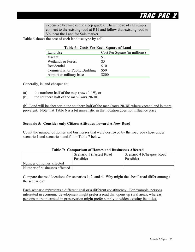
TRAC PAC 2

Activity 2 Pages 55

expensive because of the steep grades. Then, the road can simply connect to the existing road at R19 and follow that existing road to V6, near the Land for Sale marker.

Table 6 shows the cost of each land use type by cell.

Table 6: Costs For Each Square of Land Land Use Cost Per Square (in millions) Vacant $1 Wetlands or Forest $5 Residential $10 Commercial or Public Building $50 Airport or military base $200

Generally, is land cheaper at: (a) the northern half of the map (rows 1-19), or (b) the southern half of the map (rows 20-38) (b) Land will be cheaper in the southern half of the map (rows 20-38) where vacant land is more prevalent. Note that Table 6 is a bit unrealistic in that location does not influence price. Scenario 5: Consider only Citizen Attitudes Toward A New Road Count the number of homes and businesses that were destroyed by the road you chose under scenario 1 and scenario 4 and fill in Table 7 below.

Table 7: Comparison of Homes and Businesses Affected

Scenario 1 (Fastest Road Possible)

Scenario 4 (Cheapest Road Possible)

Number of homes affected Number of businesses affected Compare the road locations for scenarios 1, 2, and 4. Why might the “best” road differ amongst the scenarios? Each scenario represents a different goal or a different constituency. For example, persons interested in economic development might prefer a road that opens up rural areas, whereas persons more interested in preservation might prefer simply to widen existing facilities.

TRAC PAC 2

Activity 2 Pages 56

STUDENT GOAL FOR ACTIVITY 2 Your goal is to pick the “best” road for connecting cells A38 and Z1. You want to choose the best road type, design speed, and location so that you please everybody: taxpayers who want a cheaper road, residents who want a road close to their homes but not through their homes, drivers who want a road that is fast, pedestrians who want to be able to walk safely, the airport authority who wants direct access, and so on! Use the following five steps as a guide for picking the “best” alignment. 1. Place a yellow Post-it note at the starting point (A38), the ending point (Z1), and on any

other locations where the road must go. Put a green smiley face☺ on those notes.

Figure 9: A “Smiley Face goes in the lower left hand corner of this map bottom (cell A38)

2. Place a yellow Post-It note on any locations where the road absolutely cannot go, such as

the Federally protected Great Dismal Swamp (H18). Put a red X on those notes.

TRAC PAC 2

Activity 2 Pages 57

Figure 10: A Red X Goes on the Great Dismal Swamp at cell J18

3. Identify any areas that you prefer not be affected by noise or runoff from the road, such

as the Snake River from the upper map in Figure 9. Encircle these areas very lightly in pencil. This buffer should be at least two cm from the area for a two lane road, four cm for a four lane road, and six cm away for a six lane road, as suggested in Figure 11 below.

Hint: The buffers are different sizes because larger roads will have higher traffic volumes that leave a greater environmental footprint.

Figure 11: Example of Different Buffer Areas for Snake River

4. Pick a road type that can accommodate demand. During a typical day, demand for the

road varies between 3,000 and 12,000 vehicles per hour as shown in the table below.

TRAC PAC 2

Activity 2 Pages 58

Table 8: Hourly Demand for the Road

Hours of the Day Volume of drivers who would like to use the road 7:00 - 8:00 am 10,000 10:00-11:00 am 6,000 1:00 - 2:00 pm 3,000 4:00 - 5:00 pm 9,000 6:00 - 7:00 pm 12,000

5. Lay out the road on the map, using the appropriate transparent tangent sections and the

curved sections. Change the road type, design speed, or location until the road does all of the following:

intersects all of the green smiley faces (step 1) avoids all of the red Xs (step 2) touches few or none of the penciled-in buffer areas (step 3) moves enough people (step 4)

You can redo steps 1,2,3, and 4 until you are satisfied with your proposed road. Do not turn the page over unless you cannot do step 5 within 5 minutes time.

TRAC PAC 2

Activity 2 Pages 59

Hint for Step 5 on page 58.

If you cannot complete step 5, then you may want to change one of your answers for steps (1-4). For example, if you originally had many protected areas in step (2), then you might now want to unprotect some of those areas, enabling more possible road locations.

EVALUATION QUESTIONS: IS ANYONE HAPPY WITH YOUR DESIGN? Suggested answers for activity 2 evaluation questions are in the Teacher Reference on page 10. 1. Were you able to meet all of your original criteria in the steps (1)-(4) or did you

have to change your answers to steps (1)-(4)? (a) My road met all of my original criteria in steps (1)-(4) (b) I had to change my criteria in step (1), (2), (3), or (4) to build the road 2. Determine the total cost of the road by adding the costs of the individual cells. This

can be done by hand or it can be done with the spreadsheet software. The cost is $_______ in millions

3. Determine the environmental impacts by counting the cells inside any buffered areas from step 3 (such as the Snake River).

A total of ________cells are affected by runoff or noise pollution. 4. Indicate the number of homes and businesses that will be displaced by the road _______homes will have to be relocated

_______businesses will have to be relocated

5. What percentage of the time will your road have enough capacity to avoid a traffic jam (e.g. breakdown conditions)? (See Tables 2 and 8).

_______% of the time we will not have a traffic jam

Table 8: Hourly Demand for the Road Hours of the Day Volume of drivers who

would like to use the road Capacity of the Four Lane 50 mph Arterial


7:00 - 8:00 am 10,000 6,400 No 10:00-11:00 am 6,000 6,400 Yes 1:00 - 2:00 pm 3,000 6,400 Yes

TRAC PAC 2

Activity 2 Pages 60

Hours of the Day Volume of drivers who would like to use the road

Capacity of the Four Lane 50 mph Arterial


4:00 - 5:00 pm 9,000 6,400 No 6:00 - 7:00 pm 12,000 6,400 No 6. Indicate which goal is best achieved by your road (Tables 3 and 4 may be helpful). (a) move a lot of traffic (b) minimize environmental impacts such as water runoff and noise (c) consume as little land as possible (d) increase pedestrian safety (e) encourage economic development in rural areas. 7. Indicate which of the following constituents is likely to be the most content with the

construction of the road. (Table 5 may be helpful). (a) residents (____________________________________name the particular areas) (b) through travelers that do not live in the community (c) small business owners (__________________________name a few that apply) (d) The Western Forest Preserve Conservation Society (e) the Airport Authority 8. What can you conclude is the “best” decision for this community if they decide they

want a new road? ______________________________________________________________________ ______________________________________________________________________ 9. The location for a road that is guaranteed to make all citizens happy is probably

(a) in a rural area (to encourage economic development) (b) in an urban area (so as to preserve farmland) (c) in the mountains (to provide a scenic view) (d) within driving distance of major residential neighborhoods (e) probably no location will please everyone!

10. What mode of transportation was not fully considered in this example (but should

be considered in real life)?

(a) bicycle (b) walking (c) public transportation (buses) (d) public transportation (light rail or “subways”) (e) all of the above

TRAC PAC 2

Activity 3 Pages 61

ACTIVITY 3: HOW MUCH DOES IT COST?

ACTIVITY TABLE Teacher Prep Time 15 minutes In Class Time 45 minutes parts A, B, and C

45 minutes discussion and questions Grade/Course HS Mathematics Technology High National Council of Mathematics Teachers Standard

Data Analysis and Probability

INTRODUCTION This activity enables students to use tools common in the workplace to develop a mathematical model that can make predictions. The transportation concepts of estimating right of way costs for different pieces of property are covered. Students classify property by land use and location and then predict the selling price of these properties using a mathematical model they develop themselves. Although any spreadsheet package such as Microsoft Excel may be used, we recommend Activity 3 be done with the supplied software (Vernier Graphical Analysis). OBJECTIVE Students learn how to create, evaluate, and use a mathematical model that predicts a dependent variable (land costs) as a function of an independent variable (such as location or land use type). BACKGROUND Many empirical relationships, such as the price of a house with respect to its size and location, the salary one receives with respect to one’s abilities and the market, or the fuel economy of a vehicle given its weight, are probabilistic. The relationship is not exact but instead there is some natural variability in the answer. For example, two homes may both be located in the same exact neighborhood, may be for sale at a time when the economy is doing well, and may be of similar construction, yet their prices may be different. This is because the multitude of factors affecting the home price are not fixed but instead are variable: for example, one seller may be more willing than another to part with her home when an offer is slightly below the asking price. The

TRAC PAC 2

Activity 3 Pages 62

opposite of a probabilistic relationship is a deterministic relationship where the answer is exactly known, such as the relationship Force = (mass)(acceleration). MATERIALS Required Optional map used in Activity 2 (supplied) Vernier Graphical Analysis (supplied) data file constru3.dat (supplied)

a spreadsheet package in lieu of Graphical Analysis data file constructionactivity3.xls (supplied)

SETUP AND PROCEDURE (WITH MAP ALONE) Give each pair of students the map that was used in Activity 2. Answers to the next four questions may either be written on the board or quickly discussed aloud. Their goal is to prepare students to develop a model that predicts land price as a function of location. 1. What factors influence the price of a given piece of property (say a square on a map)?

At least two factors: the location and the type of development.

· Location may refer to the distance of the property from other land uses. For example, it may be desirable for a major airport to be located far from homes (in order to minimize noise for residents) but very near a factory (because of the airport’s ability to transport freight from the factory).

· Type of development means that some land uses are easier to replace than others. For

example, it is easier to purchase an acre of farmland than an acre containing a school. 2. Suppose you believe that the closer a cell is to the center of the map, the more valuable

it is. How might you quantify closeness of the property to the center?

· One method is to use the distance of each cell from the center of the map. Given that there are 38 rows, then, the vertical center of the map is the middle line between rows 19 and 20, which we can call 19.5. Similarly, with 26 columns, we can say the horizontal center is 13.5. Thus the center may be described as a point at row 19.5, column 13.5.

· The distance from any cell may be described as the distance of the cell from row 19.5 and

column 13.5. One way to describe this distance is with the following formula

2 2cell distance from center = (cell row - 19.5) + (cell column - 13.5)

TRAC PAC 2

Activity 3 Pages 63

Tip: If students do not know why this formula is necessary, then hold up a map and point to one cell that is 11 squares away horizontally and one square away from the center vertically. Then point to another cell that is 6 squares away vertically and 6 squares away horizontally. Ask students why the second cell is closer. The diagonal distance is accounted for in the above formula.

3. How would you rank the costs for each of the land uses shown below if they all had the

same location and occupied the same amount of space?

Costs For Each Acre of Land Land Use 500 acres of commercial 500 acres of wetlands or forest 500 acres of airport or military base 500 acres of residential 500 acres of farmland

Beginning from lowest to highest, for example, one possible ranking might be as follows:

Land Use Rank 500 acres of farmland 1 (cheapest) 500 acres of wetlands or forest 2 500 acres of residential 3 500 acres of commercial 4 500 acres of airport or military base 5 (most expensive)

4. What are the limitations of predicting land use costs based on the assumptions in

questions 2 and 3 above?

· Location and type are only two of many factors that affect the price of a piece of property. The economy, the quality of the property (e.g. how well a home is constructed), external influences (such as the quality of the school district), and the availability of water and sewer lines are other factors that influence price.

· Location can also mean the distance to other desirable (or undesirable!) land uses. A

residential home that is near a factory may not be worth as much as a residential home that is next to a park. Often, commercial land that is on a high-volume, high-capacity road is worth more than commercial land that is not near such a road, because of the extra business the road will bring as well as its ability to move employees and freight.

· Price is not the same as value. Just because an apple orchard might sell for less than a

hotel does not necessarily mean it is worth less than the hotel to the community.

TRAC PAC 2

Activity 3 Pages 64

STUDENT GOAL FOR ACTIVITY 3 Your job is to attempt to forecast what the “missing” land prices would be, using what you know about the existing land prices. To achieve this, you can develop a mathematical model that forecasts these prices as a function of the location and the type of property. SETUP (WITH MAP AND SPREADSHEET) Start the spreadsheet package and open the file constru3.dat (if using Vernier Graphical Analysis) or the file constructionactivity3.xls (if using Microsoft Excel). Both files should be located within the construction/Act3 subdirectory. Installation instructions are on page 4. The file contains three data sets:

· VacantLand (contains only cells with either farmland or no structures) · CommercialLand (contains only cells that are used commercially) · AllLand (contains all cells regardless of the type of land)

Examine the AllLand data set (scroll to the far right in Graphical Analysis). The AllLand data set is organized as follows with each row representing a cell on the map:

· row represents the row where the cell is located · column indicates the column where the cell is located (1 to 26 corresponding to A to Z) · cell indicates the cell number from 1 (row 1 column A) to 988 (row 38 column Z) · landuse indicates one of five possible land uses for the cell (see Figure 1 which

corresponds to the large maps you used for Activity 2)

1 vacant or farmland 2. environmental areas: lakes, rivers, wetlands, forest, mountains, or valleys 3. residential 4. commercial or public (businesses, roads, resorts, gas stations, malls, parks, The

OldTown Canal) 5. airport or military base

· cellcost indicates the actual cost of the land in each cell

The two other datasets VacantLand and CommercialLand are subsets of this first data set. Now go to the VacantLand dataset (scroll to the far left in Graphical analysis).

TRAC PAC 2

Activity 3 Pages 65

1234567891011121314151617181920212223242526272829303132333435363738

A B C D E F G H I J K L M N O P Q R S T U V W X Y Ze e e e e e e e e e e e e e c c c c c c c e e e e ee e e c c c c c c c c c c c c c c c c c c v v v v ve e e c c v c c c c c c c c v c c c c v c v v v v ve v v c c c c c c c c c c c c v v c c v v v v v v ve v a a a c c c c c c c c c c c c c c c c c v v v ve e a a a a c c c c c c c c c c c c c c c c c c c ce e a a a a c c c c c c c c c c c c c c c c c c c ce e a a a a c c c c c c c c c c c c c c c c c c c ce e a a a a c c c c c c c c c c c c c c c c c c c ce e a a a a c c c c c c c c c c c c c c c c c c c ce e a a a c c c c c c c c c c c c c c c c c c c c ce e a a a c c c c c c c c c c c c c c c c c c c c ce e a a a c c c c c r r r r r r r c c c c c c c c ce e a a a c c c c c r r r r r r r c c c c c c c c cv e e e e v c c c c r r r r r r r c c c c c c c c cv e e e e e c c c c r r r r r r r c c c c c c c c cv e e e e e e e e e r r r r r r r c c c c c c c c cv e e e e e e e e e r r r r r r r c c c c c c c c cv e e e e e e e e e r r r r r r r c c c c c c c c cv c c c c c c e e e e e e e r v c c c c c v v e e vc c c c c c c e e e e e e e e c c c c c e e e e e ec c c c c c v v v r e e v e e e c c v v e e e e e ec c c c c c c c c c c r r e e e r r r e e e e e e vv v c c c c c c c c c r v r e e e r r e e e e e e vc c c c c c c c c c c r r v r e e e e e e e e e e ee r r v v r v v r v r r r e e e e e e e e e e e e ee e e v v r e e e e e c r e e e e r v c c c c e e ve e e e e e e e e r r c c c c e e r v c c c c v r ve e e e r c c c c c c c c c c v e e r c c c c v r ve e c c v c c c c c c c c c c r e e v v v v v v v vv c c c c c c c c c c c c e c c c c c c c c c c c cv c c c c c c c c c e e e e e v r e e r r c c c c cc c c c c c c c c c e e e e e v r e e r v c c c c cv v v v v v v v e e e e e e v v r e e r v r c c v cv v v v v v v v v e e e e e e v r e e e r r v v v cv v v v v v v v v e e e e e e v v v e e e v r v v cv v v v v v v v v e e e e e e v v v e e e e r e e cv c c c c c c c c c c c c c c c c c c c c c c c c c

Figure 1: Color Coded Map of Land Uses PROCEDURE (WITH MAP AND SPREADSHEET) Part A: Determine how far each cell is from the prime location The map shows that the most populous areas are not clustered neatly around the physical center of the map. However, there is clearly a tendency for areas to be more populated near the top of the map (e.g. row 5) than near the bottom of the map (say row 30).

TRAC PAC 2

Activity 3 Pages 66

Where does the historic district seem to be centered? Although there are many possible prime property locations, for this exercise let’s assume that the “prime location” is centered at cell L5. That is, all other things being equal, property tends to be more expensive as one gets closer to this location of L5. Alternatively, as one goes further from L5, then property tends to be cheaper, assuming that the only factor influencing a piece of property is location. Thus our prime location is row 5 and column 12 (since “L” is the 12th letter of the alphabet) How can one compute the distance of each cell from the prime location? The distance of each cell from this prime location is given as

2 2cell distance from prime location = (cell row - 5) + (cell column - 12) Add a column to the data file that computes distance from this prime location. In Graphical Analysis, this can be done as follows after opening the file constru3.dat :

Go to the data set VacantLand. (VacantLand contains only the cells that are classified as vacant or farmland, that is, the cells with landuse = 1).

Select Data/New Column/Calculated (as shown in Figure 2), name the column distance, and give the formula for the distance from each cell as (("row"-5)^2+("column"-12)^2)^.5

Figure 2: Adding a column to compute the distance in Graphical Analysis

TRAC PAC 2

Activity 3 Pages 67

You should now have a column that shows the distance of each cell from the prime location L5. Part B: Determine a model for the cost of vacant land Examine the column to the far right that shows the price for each cell. There is some type of relationship between cost and location, but it may be difficult to pinpoint the relationship from looking at the numbers alone! Prepare a graph that shows the cost of the cell as a function of the distance from the center of the map. To do this in Graphical Analysis, double-click on the graph to the far right, select More X-Axis Options, check “distance”, click o.k., and then select More Y-Axis Options, check “cellcost”, as shown in Figure 3 below. X-Axis Setup

Figure 3: Producing a graph of CellCost Vs. Distance in Graphical Analysis

The result is that one has a graph of the relationship between cell costs and the distance of the cell from the center, as shown in the right hand portion of Figure 3. What is the general relationship between cost and location for cells with landuse = 1? Attempt to find a mathematical model that will predict the cost of vacant land as a function of the distance from the prime location. What types of models might seem most appropriate?

TRAC PAC 2

Activity 3 Pages 68

One possibility is to realize that the center distance is inversely proportional to the cost of the cell, that is, as the distance from the center goes up, the cost of the cell goes down. For example, a model that uses this inverse relationship might be “the cost is 99 divided by the distance, such that as the distance increases beyond 1, the cost drops proportionately.” This model is

99cell cost = cell distance from prime location

To see how well this model might work, select Analyze/Manual Curve Fit/y=A/X and change the parameter A to 99 as illustrated in Figure 4a below. The line reflected by this equation has the same general trend as the actual data, but it does not mirror the actual points very well! However, a better fit can be obtained with some experimenting: if we modify the equation above such that the 99 becomes a 30, then a better fit is obtained in Figure 4b below.

Figure 4a: Curve Fit with Cost=99/Distance Figure 4b: Curve Fit with Cost=30/Distance Yet notice that in both cases the fitted line does not slope as sharply as the plotted points. Select Cancel and then choose Analyze/Manual Curve/y=A/X^2 option to obtain a slightly better fitting line! You can try this for yourself, as shown in Figure 5.

TRAC PAC 2

Activity 3 Pages 69

Figure 5: Curve Fit Option with Cost=150/Distance Squared

If the expression

2

Acell cost = (cell distance from prime location)

is better than 1

Acell cost = (cell distance from prime location)

then what do you think needs to be done to the exponent to make cost function more accurate? You can try a larger exponent in the denominator: in fact, as shown in Figure 6, an excellent fit is obtained from using the expression

3

1000cell cost = (cell distance from prime location)

(To reproduce Figure 6, you still will select Cancel followed by Analyze/Manual Curve/y=A/X^2 and then manually change the italicized 2 to a 3).

TRAC PAC 2

Activity 3 Pages 70

Figure 6: Curve Fit Option with Cost=1000/Distance Cubed

In this instance, the model says the cost for a vacant square of land can be estimated as 1000 divided by the cube of the distance of that land from location L5. Realistically, one would never expect a model to work perfectly like this one did: normally land prices are affected by many other factors besides location, such as the land market or interest rates. However, it is realistic to expect that in some instances trying different kinds of models can lead to a better understanding of the relationships between variables that interest us, such as the cost of a piece of land and where it is located. Modify the distance value for cell L5 in the CommercialLand Data Set Now go to the CommercialLand Data set, cell 116 (row 5 column 12) as shown in Figure 7. The distance value should be zero. Change the row and column to 5.5 and 12.5 such that the distance value increases above zero. (We will see in part (c) why this is necessary).

(If “5.5” appears as a “6”, do not panic: the value “5.5” is still stored. You can change how it appears: select Data, then Column Options, and then CommercialLand: Row, and then under Rounding choose “1” for the number of decimals to be displayed. This step, however, is optional: the value “5.5” is recorded nonetheless.)

TRAC PAC 2

Activity 3 Pages 71

Figure 7: Changing the Row and Column Values for Cell L5 in the CommercialLand Data Set

Part C: Determine a model for all commercial land If you are using Graphical Analysis, there is actually more data in the spreadsheet than you can currently see. Go to Window/Data Table Options as shown to the left of Figure 8, and then click the mouse to add checkmarks to MegaMall, MegaMart, and Missing, which are shown to the right of Figure 8. These columns will now be visible in the data table.

Figure 8: Making the MegaMall, MegaMart, and Missing Columns Visible

The last challenge is to predict the cost of commercial land as a function of the distance from the prime location (L5). Thus the distance values you have computed and placed in the column distance will be helpful. However, commercial property prices may be much more variable than prices for vacant land. Thus follow the suggested steps below to develop your best model that predicts the price of commercial land based on its distance from the prime location of cell L5.

· Select only the cells classified as commercial (that is, the cells with landuse = 4) by going to the CommercialLand data set in Graphical Analysis.

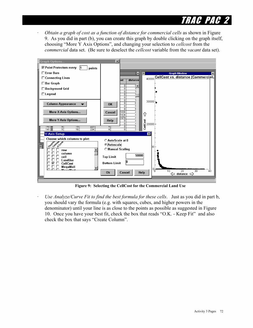
TRAC PAC 2

Activity 3 Pages 72

· Obtain a graph of cost as a function of distance for commercial cells as shown in Figure 9. As you did in part (b), you can create this graph by double clicking on the graph itself, choosing “More Y Axis Options”, and changing your selection to cellcost from the commercial data set. (Be sure to deselect the cellcost variable from the vacant data set).

Figure 9: Selecting the CellCost for the Commercial Land Use

· Use Analyze/Curve Fit to find the best formula for these cells. Just as you did in part b,

you should vary the formula (e.g. with squares, cubes, and higher powers in the denominator) until your line is as close to the points as possible as suggested in Figure 10. Once you have your best fit, check the box that reads “O.K. - Keep Fit” and also check the box that says “Create Column”.

TRAC PAC 2

Activity 3 Pages 73

Figure 10: Choosing the Best Fit as 30,000/Distance Squared

· Compare the “missing” costs to your predicted costs. As shown in Figure 11, compare

the values for each cell’s predicted costs (based on your formula) and the actual costs (shown as the variable missing). For example, for the first row in Figure 11, the formula predicted a value of 1200, whereas the actual value (shown as missing) was 1249.

Figure 11. Comparison of missing data values and predicted data values

TRAC PAC 2

Activity 3 Pages 74

· Assess how well your model works! If your model were perfect, then the prices shown in Fit 1 would be exactly the same as the prices in the Missing or CellCost columns. You can create a graph that shows the accuracy of your predictions by doing the following:

-- Create a new column by going to Data/New Column/Manually Entered -- Name the column “MyPrice” (or any name you want!) -- Copy the data from “Fit 1” to “MyPrice”

(This can be done by placing the cursor on the “Fit 1” title, clicking to highlight the column in black, choosing Edit/Copy Data, clicking on the “MyPrice” title to highlight that column in black, and choosing Edit/Paste Data)

-- Create another new column by going to Data/New Column/Calculated -- Name the column “TruePrice” (or again any name you want!) -- The New Column formula should be “CellCost” + “Missing” and press o.k. (This will create a column that has all the correct values) -- Double click on the graph to the right -- Change the X-axis from “distance” to “MyPrice” (or the name you chose above) -- Change also the Y-axis from “cellcost” to “TruePrice” (or the same name you chose) -- Change also the X and Y scales to be the same (e.g. 0 to 1000 or 0 to 30,000)

You may see a graph similar to what is shown in Figure 12a, where each point represents a comparison of the predicted price (MyPrice) to the actual value (TruePrice). If you now change the X-axis from MyPrice to TruePrice, you obtain a graph similar to what is shown in Figure 12b, which indicates a perfect fit.

Figure 12a: TruePrice vs. MyPrice Figure 12b: TruePrice vs. TruePrice

Ask students now what would happen if their distance had been “zero”, as it was originally for the commercial property in cell L5.

TRAC PAC 2

Activity 3 Pages 75

Evaluation Questions *Questions 2, 6, and 7 require more spreadsheet work and may be omitted if time is short. Suggested answers for these evaluation questions are in the Teacher Reference on page 13 1. Suppose one is comparing different models and one produces a graph of true prices

versus predicted prices as shown in Figure 12a above. How will the graph for a more accurate model compare to the graph for a less accurate model?

_______________________________________________________________________

_______________________________________________________________________

*2. For the Mega Mall of America, the total cost is given by summing the costs for cells

G7..J10. What is the total cost that your model predicts?

Hint: The column “MegaMall” has a “1” in it for those cells that have the Mega Mall. Insert a column to the right and give it a calculated formula such as

“MegaMall”*(“30000/”distance”^2) Then, go to Window/Data Table Options and check “Show statistics.” For this new column you just created, the mean multiplied by the Number will yield the total price.

The predicted cost is $________

3. Suppose that Mega Mall actually sells for $20,000. How accurate is your model?

The actual cost is $20,000__

The predicted cost is $________ (insert your answer from question 2 above)

The difference is $________

The percent error is the difference divided by the actual cost and multiplied by 100.

The percent error is ________% 4. Suppose a real estate agent wants a model that can predict costs within 25% of their

actual value. Based on the performance with the MegaMall of America, is your model accurate enough? ___yes ___no

TRAC PAC 2

Activity 3 Pages 76

5. Using the Mega Mall as an example, why might a model that predicts cost as even be of

value? Why not just ask the owners of Mega Mall directly?

_______________________________________________________________________

_______________________________________________________________________

Land prices are influenced by the proximity of transportation infrastructure. Land adjacent to a busy freeway may appeal to a business that wants customers. Yet, land prices can also be depressed by a highway location: a high speed freeway that cuts through a neighborhood and increases noise can reduce home prices. Prices can move subtly: a new light rail line can increase the price of nearby farmland if it can be converted to residential use.

Suppose it is argued that commercial land is worth more when it is near a road. In fact, a model is proposed that the value of commercial land should be equal to the following:

2

50,000One Cell of Commercial land = distance from the road

*6. What is the value of the MegaMart shown in cells X10..Z11 using the above formula?

Hint: MegaMart is designated with a “1”, as shown for cells X10..Z11. Use the spreadsheet to create a new column where each cell of MegaMart has the formula “MegaMart”*50000/(1^2) since 1 is the distance of MegaMart from the nearest road.

$_____

*7. What would be the value of MegaMart if it were located 5 units from the road rather

than just 1 unit?

Hint: Change the “1” in the above formula to a “5” since the distance is now 5 units from the road

$_____

8. If this model were accurate, then what effect can transportation proposals have on real

estate prices?

_______________________________________________________________________

_______________________________________________________________________

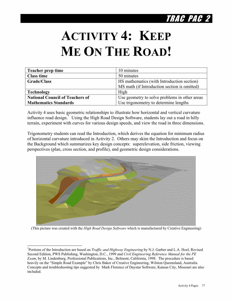
TRAC PAC 2

Activity 4 Pages 77

ACTIVITY 4: KEEP ME ON THE ROAD!

Teacher prep time 10 minutes Class time 50 minutes Grade/Class HS mathematics (with Introduction section)

MS math (if Introduction section is omitted) Technology High National Council of Teachers of Mathematics Standards

Use geometry to solve problems in other areas Use trigonometry to determine lengths

Activity 4 uses basic geometric relationships to illustrate how horizontal and vertical curvature influence road design.* Using the High Road Design Software, students lay out a road in hilly terrain, experiment with curves for various design speeds, and view the road in three dimensions. Trigonometry students can read the Introduction, which derives the equation for minimum radius of horizontal curvature introduced in Activity 2. Others may skim the Introduction and focus on the Background which summarizes key design concepts: superelevation, side friction, viewing perspectives (plan, cross section, and profile), and geometric design considerations.

(This picture was created with the High Road Design Software which is manufactured by Creative Engineering)

*Portions of the Introduction are based on Traffic and Highway Engineering by N.J. Garber and L.A. Hoel, Revised Second Edition, PWS Publishing, Washington, D.C., 1999 and Civil Engineering Reference Manual for the PE Exam, by M. Lindenburg, Professional Publications, Inc., Belmont, California, 1998. The procedure is based heavily on the “Simple Road Example” by Chris Baker of Creative Engineering, Wilston Queensland, Australia. Concepts and troubleshooting tips suggested by Mark Florence of Daystar Software, Kansas City, Missouri are also included.

TRAC PAC 2

Activity 4 Pages 78

Introduction: Horizontal and Vertical Curvature Imagine roller skating around a flat track. As you skate faster, there will be a tendency for you to be pushed away from the center of the track, and this tendency, or force, is known as the centrifugal force. A truck driving around a curve faces the same scenario: Figure 1 shows the centrifugal force pulling the truck to the right (away from the center). Fortunately, there is friction between the tires of the truck and the road, which contributes to an inward radial force that helps keep the truck from being pushed outward.

Figure 1: Radial Forces Acting on a Truck Rounding a Curve

Unfortunately, this inward radial force is not enough to keep the truck on the road. In fact, you may have noticed the same problem if you sprint around a small indoor track -- if you go too fast, you hit the outer wall! Just as an indoor track may be banked, or raised on the outside edge, so a road may have its outer edge slightly raised to keep centrifugal acceleration from pulling the truck off the road. Raising this outer edge is known as superelevation. Figure 2 shows how forces from superelevation and the inward radial force, can keep vehicles on the road in spite of the centrifugal force. The angle with which this outer edge is raised is shown as θ in Figure 2.

Hint: What is the value of θ in Figure 2? What is the value of θ in Figure 1?

In Figure 2, θ has an unrealistically large value of about 30 degrees; in Figure 1, θ had a value of zero degrees since the outer edge of the road was not elevated at all.

centrifugal force

inward radial force

Θ

Force from superelevation Figure 2: Using Superelevation to Keep the Truck on the Road

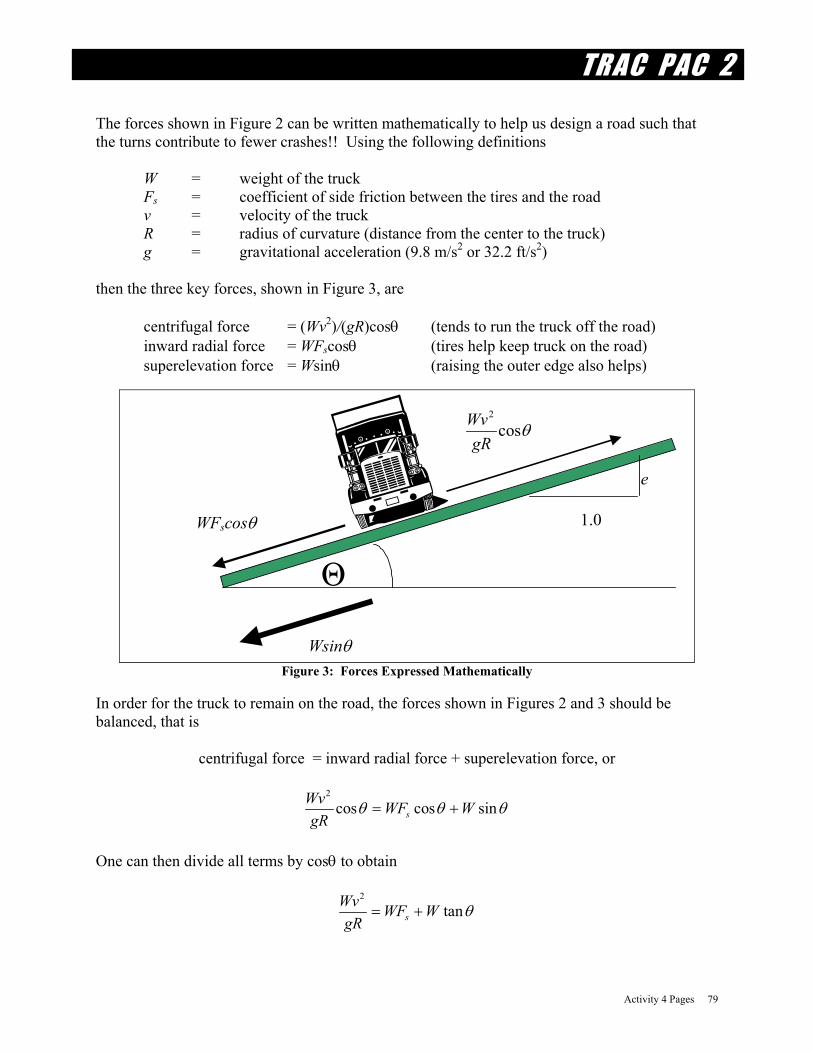
TRAC PAC 2

Activity 4 Pages 79

The forces shown in Figure 2 can be written mathematically to help us design a road such that the turns contribute to fewer crashes!! Using the following definitions W = weight of the truck Fs = coefficient of side friction between the tires and the road v = velocity of the truck R = radius of curvature (distance from the center to the truck) g = gravitational acceleration (9.8 m/s2 or 32.2 ft/s2) then the three key forces, shown in Figure 3, are centrifugal force = (Wv2)/(gR)cosθ (tends to run the truck off the road) inward radial force = WFscosθ (tires help keep truck on the road) superelevation force = Wsinθ (raising the outer edge also helps)

2

cosWvgR

θ

Wsinθ

e

WFscosθ

Θ

1.0

Figure 3: Forces Expressed Mathematically

In order for the truck to remain on the road, the forces shown in Figures 2 and 3 should be balanced, that is

centrifugal force = inward radial force + superelevation force, or

2

cos cos sinsWv WF WgR

θ θ θ= +

One can then divide all terms by cosθ to obtain

2

tansWv WF WgR

θ= +

TRAC PAC 2

Activity 4 Pages 80

where tanθ is simply the rate of superelevation, shown as e in Figure 3, such that

2

sWv WF WegR

= +

Dividing both sides of the equation by W and solving for R, one obtains

( )2

s

vRg F e

=+

Letting v be measured in km/h and letting gravitational acceleration g be 9.8 m/s2, the equation for determining the minimum radius R may be rewritten after conversion as

( )2

127 s

vRF e

=+

where v is km/h, R is in m, and Fs and e are decimals between 0 and 1

With English units and gravitational acceleration as 32.2 ft/s2, the minimum value of R is

( )2

15 s

vRF e

=+

where v is miles per hour (mph) and R is in feet.

The coefficient of side friction decreases as the design speed increases, and typical values recommended by AASHTO (American Association of State Highway and Transportation Officials, a group of transportation professionals from around the U.S.)

Table 1: Recommended Coefficients of Friction Design Speed Coefficient of Side Friction Fs

48 km/h (30 mph) 0.16 81 km/h (50 mph) 0.14 113 km/h (70 mph) 0.10

Thus a horizontal curve with a large value of R is very gentle, whereas a curve with a low value of R is very sharp. [Persons who use English units may express this sharpness as the degree of curvature, defined as 5730/R, where the “5730” is obtained as (360 degrees)(100 feet)/(2π). Thus as R increases, the degree of curvature (5730/R) decreases, and the severity of the curve lessens.]

Quick Review Questions (see the equation for determining the minimum radius R) Which variable represents the design speed shown in Table 1? Which variable represents the minimum radius of curvature? As design speed increases, what happens to the coefficient of side friction? How does increased design speed affect the minimum radius of curvature? If you must have a 70 km/h design speed, how can you lower R?

TRAC PAC 2

Activity 4 Pages 81

The variable v represents the design speed and the variable R represents the minimum radius of curvature. Table 1 shows that as the design speed increases to 113 km/h, the coefficient of side friction Fs drops. Thus, both the denominator, shown as 15(Fs + e) and the numerator, shown as v2, will rise as the design speed increases, causing the minimum radius of curvature R to increase. If one must have a 70 km/h value for v, then the only way to lower R is to increase the rate of superelevation e.

In practice, the rate of superelevation is limited -- e.g. a value of e equal to 1.0 would mean a that a 24 foot wide road had its outer edge elevated 24 feet into the air! Obviously that would be infeasible -- cars and trucks would roll off this road that is at a 45 degree angle. In fact, one generally has a superelevation rate that is no greater than 0.1 -- e.g. for a 24 foot wide road, the outer edge is no more than 2.4 feet higher than the inner edge. If there is the possibility of snow or ice, then e might have to be less (e.g. 0.08) to prevent cars from sliding toward the center. Example of How to Apply the Minimum Radius of Curvature Concept Suppose one wants to have a road that can accommodate traffic at a high speed (e.g. 113 km/h). What minimum radius of curvature is required if no superelevation is used? Table 1 shows that the coefficient of side friction Fs should be 0.10. With no superelevation (e.g. e = 0.10) the minimum radius of curvature R is

( ) ( )2 2113 1,005 meters

127 127 0.10 0s

vRF e

= = =+ +

Suppose that such a large radius of curvature will destroy homes and businesses as was discussed in the second activity, and that therefore a smaller value of R is needed. What options are available to have the road be safe yet have a value of R as small as 300 m? Three options can be investigated:

· The first possibility is to raise the rate of superelevation from 0 to the maximum permissible value of 0.10. This would reduce the minimum value of R to

( ) ( )2 2113 503 meters

127 127 0.10 .10s

vRF e

= = =+ +

The reduction to almost 500 m is a great improvement, but it is not enough! · A second option is to also decrease the design speed from 70 mph to 50 mph. Along with

the 0.10 rate of superelevation, this reduces the minimum radius to

( ) ( )2 281 258 meters

127 127 0.10 .10s

vRF e

= = =+ +

TRAC PAC 2

Activity 4 Pages 82

Thus this option preserves homes and businesses but requires a reduction in speed, so one would have to post warning signs saying “sharp curve ahead” with a reduced speed limit.

· The third option would be to change the location of the road entirely such that there is no

limit on how big the curve must be. The figure below compares the effect of using a smaller radius of curvature (which only destroys a couple of homes) versus a larger radius of curvature (which affects more homes). Eliminating the curve entirely and having a 90 degree angle would preserve all of the homes (but would greatly reduce the travel speed).

Supplemental Figure: Small Radius of Curvature vs. Large Radius of Curvature

Yet just as a roadway can have horizontal curves as shown in the figure above, it can have vertical curves resulting from hills and valleys. The amount of vertical curvature affects the road for several reasons: heavy trucks may be greatly slowed down on steep inclines, drivers may not necessarily see past a crest or peak, and even the view provided by headlights can be affected by the amount of vertical curvature. This particular activity focuses on just one aspect of vertical curvature: ensuring that the incline, or slope, is not too steep. Table 2 shows the recommended maximum grades and stopping sight distances for various roadway types. Recall that for vertical curves, the grade is simply defined as the change in vertical distance divided by the change in horizontal distance. If, for example, a 500 m road starts at sea level at one end and is 25 m above sea level at the other end, then the grade is 5%.

vertical distance 25 m .05 5%horizontal distance 500 m

= = =

Hint: Students who have completed the Maglev module may wish to refer to either Caution: 6% Grade Ahead! or Graphing the Grade which discuss this same concept.

TRAC PAC 2

Activity 4 Pages 83

Table 2: Suggested Maximum Grades and Stopping Sight Distances* Design Speed Maximum Grade

(Freeways/Arterials) Maximum Grade

(Other Urban Roads) Stopping Sight

Distance 48 km/h (30 mph) not applicable 12% 61 m (200 feet) 81 km/h (50 mph) 6% 10% 122 m (400 feet) 113 km/h (70 mph) 5% 7% 191 m (625 feet)

*These are maximum, not desired, grades for mountainous terrain: large percentages of heavy trucks or longer grades would require that one have grades substantially lower than those shown in this table. In sum, roadway design is influenced by horizontal curvature and vertical curvature. Often, a tradeoff is necessary: it may be cheaper and destroy fewer buildings to construct a road with sharp horizontal and vertical curves. Yet, a designer can reduce a roadway’s hazards as well as traffic congestion with a road that has gentle (or no) horizontal and vertical curves. In practice, there is often no single, “right” answer: a community has to weigh the pros and cons of each alternative.

Background In this activity we design a road with steep horizontal and vertical curves. The road is located in hilly terrain and in order to reduce costs that would result from flattening the entire surface, a number of curves are included in the roadway. The particular software that is being used does not require students to compute the horizontal and vertical curve radii, but they should be aware of a few key concepts that are used by the High Road design software package (and that are common to other design software products). For horizontal curves, the radius of curvature (R) for horizontal curves is shown in this package simply as the curvature. The important item to remember is that as this radius of curvature decreases, your curve sharpens. If the curve is too sharp to travel safely at a given design speed, then the curve is known as being substandard. For vertical curves, you can control the grade that is set for your road depending on the design speed shown in Table 1. For example, constructing a road that has no more than a 10% grade is much less expensive than constructing a road that has no more than a 4% grade, but lower speeds (and increased traffic congestion) may result with the 10% grade, especially if your traffic stream has a lot of heavy trucks. Usually terrain is not be a smooth field; instead, there will be hills with crests and sags. A digital terrain model can be used to define this terrain, with the height and geographical location of various points defining the contours of the land. For example, if you envision a 100 square meter plot of land, then a digital terrain model might be determined by measuring the exact height of a point every 2 m as suggested in by the Xs in Figure 4. For each “X”, or point, exact location (e.g. latitude and longitude), elevation, and a description of the land at that point (e.g. gully, property line, centerline of the roadway) would be recorded.

TRAC PAC 2

Activity 4 Pages 84

X X X X X X X X X X X X X X X X X X X X X X X X X

10 m

10 m

Figure 4: Conceptual View of a Digital Terrain Model Suppose you are a bird looking at a four lane divided arterial roadway. From left to right, you might see a sidewalk on the left side, the curb and gutter of the roadway, the travel lanes on the left side, the median, the travel lanes on the right side, the right side curb and gutter, and then the right shoulder, as shown in Figure 5. Figure 5 gives the plan view of a roadway.

curb and gutter

sidewalk travel lanes travel lanes shoulder

median Figure 5: Bird’s Eye View of a Typical Roadway Section

If you imagine you are a gopher at eye level with the ground, then a cross section view of the road shows what you see in Figure 6. The cross section is also known as a typical section.

curb and gutter

sidewalk travel lanes travel lanes shoulder

median

Figure 6: Cross Sectional View of the Roadway

TRAC PAC 2

Activity 4 Pages 85

The rate of superelevation, as described in the background section, would reflect the height of the right side of Figure 7 relative to the left side divided by the width of the road, assuming of course that center of the curve is to the left of the road. Thus with the measurements as shown in the cross section view of Figure 7, the rate of superelevation would be 1 m/18 m = 0.056 = 5.6%

1 m

median

travel lanes travel lanes

18 m

Figure 7: Roadway With a Superelevation Rate of Approximately 6%

You have probably seen contours on a map -- multiple polygons that show the height of terrain as shown in Figure 8a. A profile view of a road, such as that shown in Figure 8b, indicates how a road rises and falls as a traveler moves from one point to the next. In Figure 8, a motorist going from left to right would first climb and then descend the mountain.

Peak of the Moutain

Figure 8a: Plan View of a Road Over a Mountain Figure 8b: Profile View of the Same Road Finally, the chainage gives the position a point on the road relative to one of the road’s endpoints. For example, if the road in Figure 8a is 1 km (or 1,000 m) long, the chainage of the far “left” end could be 0, the chainage of the “peak of the mountain” could be about 500, and the chainage of the far right end could be 1,000.

Materials (All materials are supplied) Required software and data files stored in the Act4 subdirectory Student Version of High Road Design Software with one High Road CD per two students Activity4.Zip (a zipped file containing two files called) --Activity4Points.txt (raw data points for the digital terrain model) --Activity4Library.rdl (data library for the digital terrain model)

TRAC PAC 2

Activity 4 Pages 86

Optional data files stored in the Act4/Answers subdirectory (useful as a reference) Step1DTM.rdd (completed file for step 1) Step2Horizonta.rdd (completed file for steps 1 and 2) Step3Vertical.rdd (completed file for steps 1, 2, and 3) Step4Section.rdd (completed file for steps 1, 2, 3, and 4) Step5Built.rdd (completed file for steps 1, 2, 3, 4, and 5) High Road installation instructions are on page 4.

Procedure Students should plan to work through the entire activity, beginning with step 1 (create the digital terrain model) and starting with the file Activity4Points.txt. The questions that students turn in focus on reasoning about the software package rather than trying to reproduce a particular road. These questions are cumulative and are located within step 5.

Hint: What if a student comes late to class? Precreated files with each of the five steps completed are stored in the answers subdirectory (e.g. Step1DTM.rdd, Step2Horixontal.rdd, and so on) if a student needs to start part way through an activity. For example, suppose a student comes late and the rest of the class has completed step 2. That student could then open the file Step2Horixontal.rdd (in which steps 1 and 2 have been completed) and begin with the directions for step 3.

TRAC PAC 2

Activity 4 Pages 87

STUDENT GOAL FOR ACTIVITY 4 In this activity we design a road in hilly terrain following these five steps:

· create a digital terrain model · set the horizontal alignment · set the vertical alignment · design a typical section (e.g. a cross section) · construct the road in three dimensions

Tip: Depending on your monitor’s resolution, some of the pictures that follow may be easier to see on paper rather than electronically.

Step 1: Create the Digital Terrain Model Start High Road (usually from Start/Programs/CreativeEngineering OR double click on the file HighRoad.exe shown on your High Road CD) and select New (then survey data source will be checked and click “OK” for text file). Within the construction/Act4 subdirectory, select the file Activity4Points.txt as shown in Figure 9a and press “OK”, at which point you will see the points shown in Figure 9b. Each point may be thought of as being similar to an “X” from your digital terrain model in Figure 4. Each point is on a separate row: the far left column is the point number, the next two columns are the equivalent of its latitude and longitude, the next column is the height, and the far right column is an abbreviation.

Figure 9a: Selecting the file “Activity4Points.Txt” Figure 9b: Contents of the file “Activity4Points.Txt” The abbreviations shown to the far right of Figure 9b denote the physical feature located at each point. For example, “SL” means “surface level” (e.g. the ground) and “FCE” means “fence line.” These abbreviations are defined in the feature library, which is stored as file Activity4Library.rdl. It is now time to link this digital data file (Activity4Points.txt) and this library of abbreviations (Activity4Library.rdl) by doing the following:

Select Edit/Convert Text File/OK Highlight Activity4Library.rdl as the feature library file as shown in Figure 10 Click the “Library” button

TRAC PAC 2

Activity 4 Pages 88

Figure 10: Selecting the Correct Feature Library

Then, you will be prompted to add “SL” to the library, which is not necessary (thus click “Ignore” in Figure 11a) but you should add “RCPIL” (pipe invert level) as shown in Figure 11b.

Figure 11a: Ignore SL Figure 11b: Add RCPIL to the Feature Library

Figure 12 shows that the pipe invert level should be joined but not contoured. (This is a man made feature rather than a contour that would reflect a measurement of terrain elevation).

Figure 12: Adding the Pipe Invert Level

TRAC PAC 2

Activity 4 Pages 89

Figure 13a shows the terrain, but you will notice there is no perimeter: the survey points are merely shown as is. You can create a perimeter by doing the following: Select Plan/Join edge points Click “automatic,” then the “Estimate” button as shown in Figure 13b, then press “OK”

Figure 13a: Initial Terrain Model Fig 13b: Choosing “Estimate” to Create the Perimeter

The result is a perimeter as shown in Figure 14a, but still the heights of the internal survey points are not yet linked. If you then choose Plan/Contours and select “OK” then the triangles shown in Figure 14b will appear. As shown in Figure 15a, you can select Plan/Contours and then vary the minor and major contour intervals to show more or fewer contour levels (e.g. Figure 15b).

Figure 14a: Resultant Perimeters Figure 14b: Interim Triangles for Setting Contours

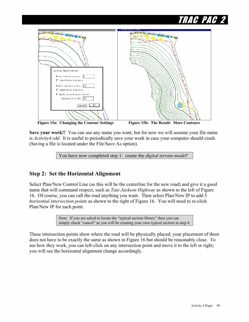
TRAC PAC 2

Activity 4 Pages 90

Figure 15a: Changing the Contour Settings Figure 15b: The Result: More Contours Save your work!! You can use any name you want, but for now we will assume your file name is Activity4.rdd. It is useful to periodically save your work in case your computer should crash. (Saving a file is located under the File/Save As option).

You have now completed step 1: create the digital terrain model! Step 2: Set the Horizontal Alignment Select Plan/New Control Line (as this will be the centerline for the new road) and give it a good name that will command respect, such as Tate Jackson Highway as shown to the left of Figure 16. Of course, you can call the road anything you want. Then select Plan/New IP to add 5 horizontal intersection points as shown to the right of Figure 16. You will need to re-click Plan/New IP for each point.

Note: If you are asked to locate the “typical section library” then you can simply check “cancel” as you will be creating your own typical section in step 4.

These intersection points show where the road will be physically placed; your placement of them does not have to be exactly the same as shown in Figure 16 but should be reasonably close. To see how they work, you can left-click on any intersection point and move it to the left or right; you will see the horizontal alignment change accordingly.

TRAC PAC 2

Activity 4 Pages 91

Figure 16: Groundbreaking Design Work for Tate Jackson Highway

By completing this second step you have completed a rough draft of the road’s horizontal alignment.

Step 3: Set the Vertical Alignment Just as you added horizontal intersection points to say where the road would fit horizontally, so you can add vertical intersection points to say where the road should be located vertically. Choose Window/Profile and then change the view so that you can see the entire profile (e.g. a view of 1:5000 should be acceptable). You will see the existing profile as shown in Figure 17.

Tip: To quickly set the scale to see the entire view, choose View/Fit to Window

TRAC PAC 2

Activity 4 Pages 92

Figure 17: The Existing Vertical Profile

Then, select Profile/New IP to add six new vertical intersection points as shown in Figure 18. You can double click on any vertical intersection point to see the chainage (e.g. the horizontal position), the grade, or the elevation as shown in Figure 19. Don’t worry if your numbers differ from those shown in Figure 18; you will change the alignment in just a few minutes.

This portion may require some experimentation with the mouse. · Once you select Profile/New IP, you can add additional vertical

intersection points simply by left clicking for each additional intersection point.

· If you accidentally delete or skip an intersection point, you can use Profile/Insert IP to make the correction.

· If an unfamiliar screen pops up similar to that shown in Figure 24b (a few pages ahead), then just delete that screen by pressing the “X” in the upper right corner. This will return you to Figure 18.

TRAC PAC 2

Activity 4 Pages 93

Figure 18: Adding 6 Vertical Intersection Points

Figure 19: Setting the Exact Height and Location of the First Vertical Intersection Point

Because there may be instances when you want to limit your grade (e.g. for safety or traffic reasons), experiment with how the profile changes if you cannot exceed a maximum value. First,

TRAC PAC 2

Activity 4 Pages 94

select Profile/Maximum Grade and then select 10%. Then grab any vertical intersection point (by placing the mouse over it and holding down the left mouse button) and move the intersection point as far up or as far down as you can: the grade can be no more than 10%. Then, move the third intersection point from the left as high as you can. The grade is of course at 10%. Now, move the second intersection point from the left higher than it originally was. Now move the third intersection point as high as you can. Why are you now able to move that point higher whereas previously you could not? Go ahead and save your work (presumably as Activity4.rdd) before continuing. It is o.k. if your profile differs somewhat from Figure 18.

With the completion of this third step you have established your vertical curvature--although you will have the chance to modify it shortly.

Step 4: Design the Typical Section (e.g. the Cross Section) The next step is to design the typical cross section (e.g. Figure 6). That is, how many travel lanes will the road have? What type of median will be present -- raised curb, grassy median, or none except double yellow lines? Are sidewalks necessary, and if so, should money be spent to place sidewalks on both sides? This fourth step culminates in the design of that typical section. Select Window/Typical Section and double click on any of the icons shown to the far left. As suggested by the left portion of Figure 20, information about each icon that you double click will appear. There are two categories of icons: “curb” icons, such as gutters and curbs (an example is shown to the left of Figure 20) and surface icons such as pavement, shoulder, sidewalk, and grass (an example of which is shown to the right of Figure 20).

Figure 20: Examples of Icons for the Typical Section View

TRAC PAC 2

Activity 4 Pages 95

Draw the cross section as shown in Figure 21, starting in the center and moving to the left for the first four subsections, or links and then returning to the center and moving to the right for the next five links. For each link, you will need to click on two icons to the left of the screen: one for the edge type and one for the surface type.* The icons for each edge type and surface type are shown in Table 3. For now, don’t worry about reproducing Figure 21 exactly, nor the shaded “crossfall (grade)” or “offset” columns. For example, so long as link 1 has edge type “mountable kerb and gutter” ( ) and surface type “pavement” ( ), that is fine. To see your typical section more easily, you may change the scale by going to View/Set Scale.

Link 5

Link 1

Link 2 Link 3

Link 4

Batterpoints

Link 6 Link 7 Link 8

Link 9

Figure 21: Left and Right Portions of the Typical Section

Table 3: Specifications for Drawing the Typical Section

Link Position Edge Type Surface Type Crossfall (Grade) Offset 1 Immediately Left of

Center Mountable kerb and

gutter

Pavement

-3 -6.1

2 Second to the Left of Center Edge + Grass 18 -2.8

*Point between links 2 and 3 Split point

3 Leftmost link (upper) §Batterpoint Grass 84 -2.6 4 Leftmost link (lower) §Batterpoint Grass -68 -2.5

5 Immediately Right of Center Edge +

Pavement

-3 4.5

6 Second to the Right of Center Edge +

Shoulder

-4 1.6

*Point between links 6 and 7 Split point

7 Third to the Right of Center Edge +

Generic ___ -54 1.6

8 Rightmost link (upper) §Batterpoint Generic ___ 82 1.235 9 Rightmost link (lower) §Batterpoint Generic ___ -54 2.893

TRAC PAC 2

Activity 4 Pages 96

*The split point does not require a surface type, rather it is used with a surface type known as batterpoint, which helps with drainage when one side of the road cuts into the earth but the other side of the road does not. §The batterpoint is a bit different from the other links: as one draws the upper link and the lower link in almost the same place (e.g. link 4 is drawn from right to left in the same spot as link 3 was).

Warning: When creating link 1, if the mountable kerb and gutter icon ( ) is embedded in the pavement as shown to the left, then click edit\undo several times to clear the screen and start again. The mountable kerb and gutter icon should be external to the pavement as shown to the right of the figure below.

Embedded External After completing your typical section with all nine links, select the arrow cursor ( )and single click on the arrow above each link, at which point a screen similar to Figure 22(a) will appear. Modify the crossfall and offset so that they match what is shown in the shaded columns of Table 3. The crossfall is the grade of the actual link from center to the far edge (so a crossfall of -3% for link 1 means that as one moves from the center of the road to the edge of the pavement, the surface slopes down at a gradual rate of 3%). The offset is the distance from the center to the edge of the link (thus there are 6.1 m of pavement as one moves from the center to the left).

Figure 22(a) Setting the Crossfall and Offset Figure 22(b) Setting the Chainage Range Finally, single click on the line that reads 0.000 – 0.000 and you will get the screen shown in Figure 22(b). Change the rightmost “0.000” to 1000,” which means that you are saying your typical section applies for a 1000 m from chainage 0 to chainage 1000. The resultant view should be similar to that shown in Figure 23, at which point you should save your work.

TRAC PAC 2

Activity 4 Pages 97

Figure 23: The Completed Typical Section

By completing this fourth step, you have designed your typical section.

Step 5: Build Your Road in Three Dimensions! Note that these questions may either be done with the file you have created (Activity4.rdd) or the answer file that currently exists (Step4Section.rdd). Suggested answers for all questions are on page 15. Select Window/Profile, View/Fit to Window, and click the left mouse button near chainage 75 as shown in Figure 24a. Release the left mouse button and a screen comparable to Figure 24b should appear. What you are seeing is a two dimensional view of how the road appears before it is built: for example, in Figure 24b, one will have to excavate quite a bit of dirt in order to lay the road! You may view use the “Go To,” “Next,” and “Previous” buttons shown in Figure 24b to see the layout of the road relative to the terrain for chainages other than 75.808.

TRAC PAC 2

Activity 4 Pages 98

Figure 24a: Profile View Near Chainage 75 Figure 24b: Cross Section View Near Chainage 75 1. Roadway sections are often referred to as either a “cut” or a “fill” section. Why do you

think that engineers refer to the section of road shown in Figure 24(b) as a cut section?

__________________________________________________________________________

__________________________________________________________________________ 2. Find the chainage for a fill section (e.g. between 0 and 1000).

__________________________________________________________________________ Select Window/Plan and then select Plan/Show Tate Jackson Highway details, and complete the dialog box as shown in Figure 25a in order to see a drawing of your proposed alignment in comparable to that shown in Figure 25b.

Make sure “All” IS checked under General in Figure 25a. Make sure “Transparent” is NOT checked in Figure 25a.

TRAC PAC 2

Activity 4 Pages 99

“Transparent” must NOT be checked

“ALL” must be checked

Figure 25a: Dialog Box for Displaying the Road Figure 25b: Plan View of the Road Tip: If the road is not yellow or red, in Plan View, select Active/Tate Jackson Highway, making

sure that you click on Tate Jackson Highway even though a check mark already appears. Experiment with showing the plan, profile, and typical section views at the same time. You can resize each of these individual views, or windows, by left clicking on the small white window in the lower right hand corner of each view (see Figure 27). To make the plan view take up the left half of the screen as shown in Figure 26, hold the left mouse button down while the mouse is in the small white box in the lower right hand corner and move the mouse up or to the left. You should use a similar technique to place the profile view in the upper right portion of the screen and the typical section view in the lower right portion of the screen as shown in Figure 26.

TRAC PAC 2

Activity 4 Pages 100

Figure 26: Seeing the Plan, Profile, and Typical Section Views at Once

You can now more easily follow the relationship between the different views. If you left click on the profile view, hold down that left mouse button, and move the resultant marker to the right, then you can see a corresponding marker move in the plan view as shown to the left of Figure 27.

TRAC PAC 2


Marker

3rd horizontal intersection point

Small, lower right, white corners to resize views.

Figure 27: A marker that shows the relationship between the plan views and the profile views

3. Look at the plan view on your screen (similar to the left side of Figure 27). As a

motorist rounds the vertex of the main horizontal curve near chainage 300, will she be going up a hill or going down a hill? How can you tell?

__________________________________________________________________________ __________________________________________________________________________

4. Given the existence of natural and man made features, what are some general reasons for why there might be a horizontal curve such as that shown in Figure 27?

__________________________________________________________________________ __________________________________________________________________________

At this point, you should save your file before you proceed further. The red sections of the road shown in Figure 27 are portions that are “substandard” because of safety reasons. Left click on the “third horizontal intersection point,” located near chainage 280 and highlighted in Figure 27. While holding the left mouse button down, move this intersection

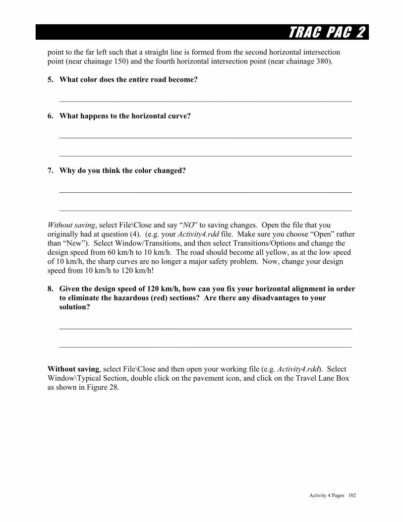
TRAC PAC 2


point to the far left such that a straight line is formed from the second horizontal intersection point (near chainage 150) and the fourth horizontal intersection point (near chainage 380). 5. What color does the entire road become?

__________________________________________________________________________ 6. What happens to the horizontal curve?

__________________________________________________________________________ __________________________________________________________________________

7. Why do you think the color changed?

__________________________________________________________________________

__________________________________________________________________________ Without saving, select File\Close and say “NO” to saving changes. Open the file that you originally had at question (4). (e.g. your Activity4.rdd file. Make sure you choose “Open” rather than “New”). Select Window/Transitions, and then select Transitions/Options and change the design speed from 60 km/h to 10 km/h. The road should become all yellow, as at the low speed of 10 km/h, the sharp curves are no longer a major safety problem. Now, change your design speed from 10 km/h to 120 km/h! 8. Given the design speed of 120 km/h, how can you fix your horizontal alignment in order

to eliminate the hazardous (red) sections? Are there any disadvantages to your solution?

__________________________________________________________________________ __________________________________________________________________________

Without saving, select File\Close and then open your working file (e.g. Activity4.rdd). Select Window\Typical Section, double click on the pavement icon, and click on the Travel Lane Box as shown in Figure 28.

TRAC PAC 2


Figure 28: Selecting the Pavement Icon as the Travel Lane

Then, select Window/Transitions, under the transitions menu select “options,” and then check both boxes. You may or may not get a warning message indicating that the “straight is too short”. For now, ignore this message and simply press o.k. Then, reposition the transitions window (using the lower right hand corner) to obtain a screen comparable to Figure 29, with the transitions window to the right and the plan view to the left.

Figure 29: Plan View and the Transitions Window

TRAC PAC 2


Save your work (e.g. as Activity4.rdd). In Figure 29, the 7% shown in red is the rate of superelevation (e) and the line that reads “Curvature” is the radius of curvature, or R, for each tangent section. For example, for the rightmost column, the current value of R is 84.3 and the current value of e is 0.07. If you go to Transitions/Options, you will see that the current design speed is 60 km/h. If you go to Transitions/Superelevation, you will see that at 60 km/h, the coefficient of side friction Fs, which is shown in this software package as f, is 0.16. Note that you may have a different value of R depending on how you placed your road. 9. Using the equation to compute the minimum radius of horizontal curvature, what

minimum value of R is necessary in order to accommodate the design speed of 60 km/h given the values of Fs and e shown immediately above?

__________________________________________________________________________ __________________________________________________________________________

10. Is your actual radius of curvature (shown in Figure 29 as 84.30) larger than the computed radius of curvature in question (9)?

_____yes ___no 11. Suppose all horizontal intersection points are fixed except the third intersection point.

Write down the actual value of R (shown in Figure 29 as 84.30) but your value may be different.

__________ Then close the transitions window. Now move this intersection point very slightly to the

left. Reopen the transitions window (Window/Transitions). Write down now this new value of R.

__________

What happened to the actual value of R as you moved slightly to the left?

__________________________________________________________________________

__________________________________________________________________________ 12. Suppose you start moving the horizontal intersection point very slowly to the left.

Using only the value of R shown in your transition view (e.g. what you have in lieu of

TRAC PAC 2


the “84.30” in Figure 29), can you predict when the roadway section will change from red to yellow?

__________________________________________________________________________

__________________________________________________________________________

Close your file (again you do not need to save your work). Then, open the file Activity4.rdd, and immediately save your file as a new name (e.g. Activity4BuildIt.rdd). Then choose Window/Plan View and then under the Plan menu choose Construct Tate Jackson Highway.

As long as you have saved your work in a different file name as done in the previous paragraph, you can ignore the terrain model warning that you receive on the screen.

Then under the Plan menu choose show camera. Move the camera as shown to the left of Figure 30 (by holding down the left mouse button and dragging the mouse) and chose a 120 m elevation (by double clicking on the left mouse button) as shown to the right of Figure 30.

Figure 30: Positioning the Camera and Setting the View

Then choose Window/3D View to see a three dimensional layout of the road. You can experiment with different perspectives by moving the camera; you should be able to see some views comparable to those shown in Figures 31 or on the first page of this activity.

TRAC PAC 2


Figure 31: Alternative Three Dimensional Layouts of Tate Jackson Highway

Optional: Create a Movie of a Vehicle Driving through the Terrain You can create a “drive through” movie that shows what it is like for one to drive on the road that has been constructed. First exit from High Road and then do the following right before lunch or some other period when the computer will not be in use for a half hour or so:

1. Make sure that the folder shown as HighRoadViewer (shown under Construction/Act4 on your Construction CD) has been copied to the hard drive.

2. Double click on the file HighRoadViewer.exe shown within the HighRoadViewer folder

on your hard drive. 3. Select “Open”. 4. Choose the file Activity4BuildIt.rdd in the Construction/Act4 subdirectory (or whatever

file you have used that actually has the constructed road). 5. Select View/Use good quality. (You may later try “better” quality, although this will take

longer to create the movie.) 6. Select View/Drive Through and then press “OK” at the next screen. 7. Enter a file name (give it a .mov extension) for your movie.

Over the next half hour the computer will create a QuickTime movie and will store the file on your hard disk. Then, after this movie has been created, you can view it with the QuickTime shareware program. (QuickTime installation instructions are on page 4.) Example movies that have already been created are shown in the HighRoadViewer folder as Activity4GoodQuality.mov and Activity4BetterQuality.mov.

TRAC PAC 2


ACTIVITY 5: TAKE THE SHORT WAY HOME!

Using Visual Basic for Applications (VBA) in Excel, students design and code a visual basic subroutine that simulates traffic speeds on two parallel routes depending on the volume of traffic. After a brief background about how a Traffic Management System (TMS) might be used to manage congestion, students take three steps toward building their own software application: design the user interface, compute traffic speeds as a function of volume, and create a simple graphical animation of traffic flow. Step (4) of this activity can be challenging if students have no experience with Visual Basic. If time is limited, such students can still work through this activity with the existing application (see constructionactivity5.xls) rather than creating their own software application. The activity concludes with vehicles moving through two signalized intersections via the SimTraffic simulation package.

ACTIVITY TABLE Teacher prep time 1 - 3 hours depending on interest and background

Familiarity with Excel is helpful for step (4) Class time Variable depending on teacher interest:

· 1 hour (step 1 only) · 4 hours (steps 2 and 3 only) · unlimited (step 4)

Students do not have to do all steps Grade/class HS Computer Science/Information Technology

HS Mathematics Technology High International Society for Technology in Education Standards

Apply simulations in real world situations


Intelligent transportation systems

TRAC PAC 2


Attention Teachers: Possible Progression Through Activity 5 Activity 5 itself is divided into four steps. Teachers have some flexibility for how to proceed with Activity 5 depending on interest in Visual Basic for Applications (VBA) and class time.

· Students who have no interest in VBA may wish to do step (1), skip steps (2) - (4), and

conclude with the SimTraffic simulation at the end of this activity. (1 hour)

OR · Students who are just beginning to learn VBA may wish to focus on steps (1) - (3), omit

step (4), and conclude with the SimTraffic simulation. (up to 5 hours)

OR · Students who wish to work with VBA in depth can do all four steps, focusing their

creativity and energy on step (4) and on improvements to the graphical interface that are outlined at the end of step (3). (unlimited time)

Table of Contents Within Activity 5

Procedure Step 1: Start the Visual Basic environment in Excel…………………………….. 115 Step 2: Design the user interface…………………………………………………. 115 Step 3: Write the code that computes speeds…………………………………….. 119 Step 4: Write the code that performs the animations (optional)…………………... 123

Discussion: What is the code doing in Step 4?……………………………………. 129 Activity 5 Evaluation Questions…………………………………………………………… 130 Optional: Simulate Poor Signal Coordination!! (Traffic Simulation Software)………….. 133

TRAC PAC 2


BACKGROUND Recall the very first construction activity where students poured popcorn through a funnel. When the popcorn jammed, the solution was to get a wider funnel -- and then the popcorn did not jam at all. Likewise, when roads become clogged with traffic, one answer is to widen existing roads. Road widening carries some disadvantages however -- activity 2 showed that roads that take property from residents, businesses, public parks, and others can often be unpopular. Additionally, roads can cause environmental problems, especially if they must go through or near water supplies, wetlands, or forests. Finally road building is expensive: construction costs can be as high as $40 million per mile of new road depending on the amount of earthwork required, the design standards, the number of lanes, and the terrain. These high construction costs have led transportation agencies to look for ways to use existing roadways more efficiently. One technique is to install sensors on the roads throughout an area, to monitor the data collected from these sensors, and to let motorists know which roads they should avoid. These sensors, along with the requisite software, help estimate average traffic volumes and speeds which are relayed to a traffic management system (also known as a “TMS”). A TMS uses real-time video monitors, simulation models, telephones, and most importantly, people, to determine where key bottlenecks are occurring. Photographs from inside one TMS in a large metropolitan area are shown below in Figures (1a) and (1b).

Figure 1a: Live Video Screens from a TMS Figure 1b: Inside the Hampton Roads TMS

(Figures 1, 2, and 3a courtesy of the University of Virginia Smart Travel Lab) Operators inside the TMS make decisions about which roads are suffering from congestion and then alert motorists through every communications medium conceivable: electronic changeable message signs that are posted on the roadway, AM radio (also known as highway advisory radio), Websites with live updates about road conditions, cable television stations, and voice mail recordings where motorists can call to find out about conditions of a particular road. Figures 2a and 2b show a changeable message sign (CMS) which can convey short messages such as “I-5 congested next 5 miles” (one screen) followed by “use instead main street” (next screen).

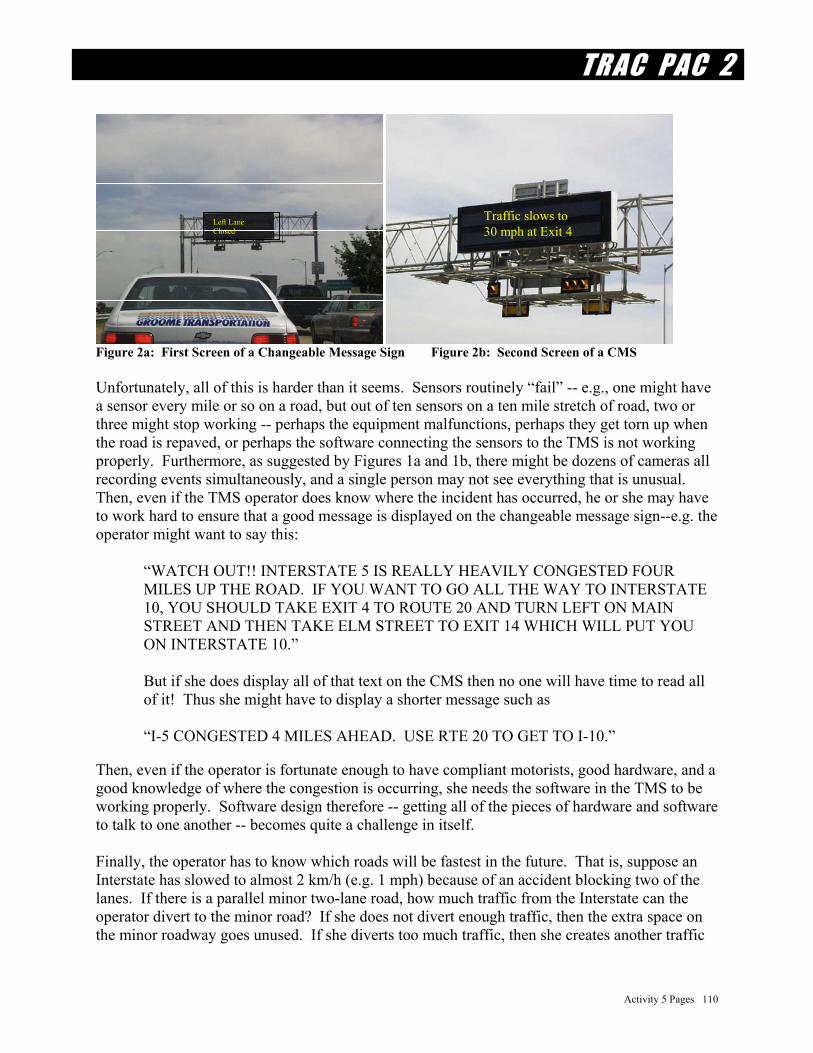
TRAC PAC 2


Left Lane Closed

Traffic slows to 30 mph at Exit 4

Figure 2a: First Screen of a Changeable Message Sign Figure 2b: Second Screen of a CMS Unfortunately, all of this is harder than it seems. Sensors routinely “fail” -- e.g., one might have a sensor every mile or so on a road, but out of ten sensors on a ten mile stretch of road, two or three might stop working -- perhaps the equipment malfunctions, perhaps they get torn up when the road is repaved, or perhaps the software connecting the sensors to the TMS is not working properly. Furthermore, as suggested by Figures 1a and 1b, there might be dozens of cameras all recording events simultaneously, and a single person may not see everything that is unusual. Then, even if the TMS operator does know where the incident has occurred, he or she may have to work hard to ensure that a good message is displayed on the changeable message sign--e.g. the operator might want to say this: “WATCH OUT!! INTERSTATE 5 IS REALLY HEAVILY CONGESTED FOUR

MILES UP THE ROAD. IF YOU WANT TO GO ALL THE WAY TO INTERSTATE 10, YOU SHOULD TAKE EXIT 4 TO ROUTE 20 AND TURN LEFT ON MAIN STREET AND THEN TAKE ELM STREET TO EXIT 14 WHICH WILL PUT YOU ON INTERSTATE 10.”

But if she does display all of that text on the CMS then no one will have time to read all

of it! Thus she might have to display a shorter message such as “I-5 CONGESTED 4 MILES AHEAD. USE RTE 20 TO GET TO I-10.” Then, even if the operator is fortunate enough to have compliant motorists, good hardware, and a good knowledge of where the congestion is occurring, she needs the software in the TMS to be working properly. Software design therefore -- getting all of the pieces of hardware and software to talk to one another -- becomes quite a challenge in itself. Finally, the operator has to know which roads will be fastest in the future. That is, suppose an Interstate has slowed to almost 2 km/h (e.g. 1 mph) because of an accident blocking two of the lanes. If there is a parallel minor two-lane road, how much traffic from the Interstate can the operator divert to the minor road? If she does not divert enough traffic, then the extra space on the minor roadway goes unused. If she diverts too much traffic, then she creates another traffic

TRAC PAC 2


jam on the minor road -- and no one will heed her messages in the future! To make this determination, an operator might use a simulation model, such as those shown in Figure (3), to decide under what conditions a road might be faster or slower than an alternative route.

Figures 3a and 3b: Screen Displays of Example Simulation Models

(Figure 3b courtesy of the Trafficware Corporation) INTRODUCTION One of the challenges that transportation professionals must wrestle with is designing, coding, and applying software. This activity focuses on designing a very simplified version of software that might be used in a TMS or in a simulation package. We will use a programming language called Visual Basic for Applications (VBA) that is included with Microsoft Excel. Although instructions are given in VBA, the same approach may be used for Visual Basic or other programming languages.) (VBA is similar to Visual Basic, which in turn was preceded by Microsoft QBasic and the older GW-BASIC. Although programmatically VBA is more “restrictive” than VB, its advantage is that it is free with Excel, which is common to both Macintosh and IBM platforms.) The purpose of this activity is to build a software subroutine that predicts traffic speed on two parallel routes (a six lane freeway with three lanes in each direction and a minor road with one lane in each direction). The software will then display a simple animation of how traffic might appear at these different volumes. Although our application will simply compare speeds on two routes, one can see how such an approach could be expanded to include sensors throughout a city or region to detect volumes and speeds on all routes.

TRAC PAC 2


STUDENT GOAL FOR ACTIVITY 5 The goal of this activity is to recreate a software application, similar to constructionactivity5.xls, which shows how traffic congestion affects traffic speed. MATERIALS AND SETUP Microsoft Excel and Office 2000 (not supplied) Example file ConstructionActivity5.xls and image files hotrod.bmp and VBcar.wmf Word file ConstructionManual.doc (so you don’t have to retype the computer code!) SimTraffic simulation package (demonstration version) and associated files This activity may be done with up to three students per computer. Software installation instructions are on page 4. Start Microsoft Excel (Start/Programs/Microsoft Excel), open the file ConstructionActivity5.xls (located within Construction/Act5) and press “Enable Macros” when prompted. A screen similar to Figure 4(a) will appear. Because the resolution of your computer may vary, you can adjust the size of the screen by selecting View/Zoom/25% (or some other percentage). Change the volume for the minor road (the road on the left of your screen) from “zero” to 800 vehicles. This means that over an hour, 800 vehicles are using the minor road. Then change the volume of the freeway (the road on the right of your screen) to 2,000 vehicles per hour, the number of simulations to 5, and the following cars per lane to “3” as shown in Figure 4(b).

TRAC PAC 2


Fig 4a: Basic Screen Fig 4b: Changed Volumes Then press “Start” to see the vehicles moving on the screen as shown in Figure 4c.

TRAC PAC 2


There are several features you may wish to consider during the simulations: Notice how the freeway shown to the right has a higher speed despite a higher volume, not only because it has more lanes than the minor road but also because the lanes themselves are designed to accommodate more traffic. You can vary the volumes for each route, and you can also notice how the vehicles on the left sometimes oscillate between being very close to one another and being far apart. Finally, the distance between the vehicles becomes closer as the speeds drop. All of these characteristics are decided not by the “computer” but rather the programmer who builds the software. For this activity, you will be the programmer. You can now exit from Excel; there is no need to save anything.

Later, in step (4), you can search for the word VBCar.wmf, replace that with hotrod.bmp and see how the bitmap image rather than the windows metafile image improves the quality of the picture.

Fig 4c: Running the simulation

TRAC PAC 2


PROCEDURE AND STEPS There are four main steps for this activity. Students who have previous experience with Visual Basic for Applications may be able to skip some of these steps or do them at an accelerated pace: 1. Start the Visual Basic for Applications environment in Excel 2. Design the user interface 3. Write the code that computes speeds 4. Write the code that performs the animation (optional) Step 1: Start the Visual Basic for Applications environment in Excel Start Microsoft Excel with (generally Start/Programs/Excel) and turn off the gridlines shown on the screen by going to Tools/Options/Views/Window options unchecking the “gridlines” box. Then select Views/Toolbars and check “Drawing,” “Visual Basic,” “Control Toolbox” such that the Drawing toolbar (shown at the bottom of Figure 5), the Visual Basic toolbar (shown to the right of Figure 5), and the Control Toolbox (shown at the Top of Figure 5) are all visible. Then check the “Design Mode” button on the Visual Basic toolbar shown in Figure 5b.

Fig 5a: Drawing, Visual Basic, and Control Toolbars Figure 5b: Checking “Design Mode”

Step 2: Design the User Interface Draw the minor road (shown to the left of Figure 6a) and the freeway (shown to the right of Figure 6a) using the different lines shown in the Drawing toolbar. Note that you can change the color, thickness, and dashing of a line by right clicking on it and selecting “Format Autoshape”. Make each lane about 1 column apart and have each line be about 75 rows long. To readily see everything, you can go to View/Zoom and check “25%” or some other zoom amount depending on your monitor size and screen resolution.

TRAC PAC 2


Hint: You can copy a line by selecting it, copying it (control-c) and pasting it (control v)

+ Fig 6a: Drawing the roads Fig 6b: Adding the “Start” button and modifying its properties Then go to the control toolbox and select the “command button” control by left clicking the mouse button. Release the left mouse button, move the mouse over to the left side of the screen, hold the left mouse button down, and draw a square which will become your command button control. Right click on the control, select “properties,” and make the following changes as shown in Figure 6(b). The name property should be “StartButton” The caption should read “Start” The font should be “Arial 36 point” or any other large font You can reposition the Start Button by holding the mouse over the center and clicking the left mouse button, or you may resize it by holding the mouse over a particular edge or corner (see the white squares in Figure 6(b)) and clicking the left mouse button. Add another command button control and place it below the StartButton control. Give this new control the name property “ResetButton”, change its caption to “reset” and also give it a large font size as shown in Figure 7.

TRAC PAC 2


Figure 7: Adding a Reset Button and Changing its Properties

Then, add a different type of control -- the label control--as shown in Figure 8. The label control button is the big ‘A’ on the Control Toolbox Bar. You should add six label controls. It does not matter what their name is, but their captions should be “volume” (for two label controls in the upper part of the screen), “speed (mph)” (for two label controls in the middle of the screen), “number of simulations” (for one label control right above the reset button), and “Following cars per lane” (for one label control in the bottom of the screen). For each control you may change the “Text Align” property to “Center”, the “Word Wrap” property to “True”, and the font to a large font (e.g. 28 or 32) as shown in Figure 8.

You can copy controls just like you copied lines previously. You can move the control by placing the mouse over the control center, holding down the left mouse button, and then moving the mouse. However, when you copy the buttons make sure that you change the relevant properties for each button. You can also resize the control by selecting it, moving the mouse to an edge, holding down the left mouse button, and then shrinking or enlarging the control.

TRAC PAC 2


Figure 8: Adding Label Controls and Changing their Properties

Next, add a type of control that will allow the user to enter a number or that will display a number to the user -- a text box control. Add five text box controls, as shown in Figure 9, and change their properties as follows: Name Font Text LeftVolume 28[or any large font] 0 RightVolume 28 0 LeftSpeed 28 [keep blank] RightSpeed 28 [keep blank] SimulationNumber 28 2

TRAC PAC 2


Figure 9: Adding TextBox Controls and Changing their Properties

This is a good place to save your work (File, SaveAs, and then pick a good file name such as RoadBlaster.xls. You should save your work every 15 minutes or so.

Step 3: Write the code that computes speeds Double click on the “Start” button and the screen will change such that you see text. At the bottom of your monitor screen you will see the green “Microsoft Excel” icon, and if you click on that you return to Figure 9. Double click on the “Reset” button and the screen changes back to the text, which is now shown in Figure 10.

TRAC PAC 2


Figure 10: Visual Basic Coding Window for the Reset and Start Buttons

This window means any code you type after the “Private Sub ResetButton_Click()” line and before the “End Sub” line will be executed when the user presses the reset button. Add the following lines of text between those two lines as shown in Figure 11(a). LeftSpeed.Text = ""

RightSpeed.Text = "" LeftVolume.Text = "0" RightVolume.Text = "0" StartButton.Caption = "Start" SimulationNumber.Text = "2" You can experiment with this code after entering it into the Visual Basic Coding Window in Figure 11(a) by returning to your main screen (e.g. Figure 11(b)), choosing the “Exit Design Mode” option shown in Figure 11(b), and then running the program by pressing the Reset Button. The purpose of this code is to clear the volume and speed boxes: if you enter a number into the volume box, the reset button will clear it.

Tip: If you get an error message which highlights a section of your code in the Visual Basic Coding Window, check that your buttons are correctly named and have the correct properties. (The code will highlight those sections that you may

TRAC PAC 2


need to recheck. Once you have corrected any errors, press the blue square reset button at the top of the coding window and then rerun the program.

Fig 11a: Visual Basic Coding Window

Fig 11b: Changing to “Exit Design Mode”

TRAC PAC 2


Return to the Visual Basic Coding Window, go to the very top, and add the following line Public Lspeed As Integer, Rspeed As Integer The two variables Lspeed and Rspeed will be the speeds for the left roadway (the minor road) and the right roadway (the six lane freeway, of which three lanes are shown). Then add the following text between the lines “Private Sub StartButton_Click()” and “End Sub”:

Dim I, J, K As Integer I = 0: J = 0: K = 0 Call Compute(Lspeed, Rspeed) StartButton.Caption = "Finished"

The third line “Call Compute(Lspeed,Rspeed) is what we will use to actually compute the speeds as a function of the traffic volume the user enters. You can enter the following text at the very bottom of the Visual Basic Coding Window and then we will see what it does:

Sub Compute(Lspeed, Rspeed) Let Lspeed = 60 * (1 - (Val(LeftVolume.Text) / 2800)) Let Rspeed = 80 * (1 - (Val(RightVolume.Text) / (3 * 2300))) Let Lspeed = CInt(Lspeed * 10 / 10)

Let Rspeed = CInt(Rspeed * 10 / 10) If Lspeed < 1 Then Lspeed = 1 If Rspeed < 1 Then Rspeed = 1 DoEvents LeftSpeed.Text = Lspeed RightSpeed.Text = Rspeed DoEvents

End Sub What is the above text doing? A rough approximation for determining speed as a function of volume is given as follows:

602800

Two Lane Road VolumeTwo Lane Road Speed =

or 802300 ( )

Freeway VolumeFreeway SpeedNumber of Lanes

=

The first four lines in the Compute subroutine estimate these speeds from the volumes the user entered (shown as LeftVolume.Text and RightVolume.Text) and then use the CINT function to round these speeds off to the nearest integer. The next two lines (If Lspeed…) ensure that a negative speed cannot occur, and the lines “LeftSpeed.Text = Lspeed” and “RightSpeed.Text = Rspeed” change the text boxes from blanks to actual speeds. To see more how these lines work, return to the main screen (e.g. Figure 11(b)), change the icon to “exit design mode” if necessary, enter different volumes (such as 400 for the minor road and 3,000 for the freeway) and press the “Start” button.

TRAC PAC 2


Hint: If you have difficulty entering speeds, volumes or making the program run, you may need to change out of design mode.

You can repeat this run several times. As you increase your volumes, you should see the speeds start to drop. After you press “Start” and get your speeds, you can press “Reset” to clear all boxes and then enter new volumes.

With the conclusion of step (3) teachers have a choice. Students who have an interest in developing algorithms can go on to do step (4). Students who want to express their creativity through designing a better user interface can revisit step (3), considering changes such as using different cars, adding intersections or cross streets to the roads, or even adding a traffic circle.

Step 4. Write the code that performs the animation (optional) The last step of this application is to design an animation such that cars move along the screen. Teachers may elect to skip this section entirely or to have students simply run the existing animation in the file constructionactivity5.xls. Students who wish to build this portion, however, can complete these instructions. First, add a list box control to your main screen by selecting “list box” from the control toolbox, placing the control immediately below the label reading “Number of cars per lane”), and change the name property of the list box to “CarsPerLane”, the “ColumnCount” to “5”, the “ListFillRange” property to “E55:E59”, the “ListStyle” to “1--fmListStyleOption”.In order to enter the numbers one through five into the list box, you have to click onto the spreadsheet so that the cursor is a square box on cell E55. (It does not matter if E55 is not where you placed your list box.) You may want to zoom in a bit in order to locate E55 easier. Enter a “1” in this block. Then enter “2” in E56, “3” in E57, “4” in E58, and “5” in E59. The list button you just created is shown at the bottom of Figure 12. To avoid an error the first time you run your program, set the Value property for your list box control to 1. Once you are finished, you can experiment with the font size and the position of your objects (such as the list box just created in the paragraph above) such that your screen, shown to the left of Figure 12, is aligned properly.

TRAC PAC 2


Figure 12: Adding a List Box Control and Changing its Properties

Second, add an image control. Figure 13 shows that you should place this control below the freeway. However, you will also need to change several of its properties: Name should be RightCar Picture is browsed to be “VBcar.wmf” (or any other picture such as hotrod.bmp) Height should be approximately 50 (40.8 was used here) Left should be around 500 (but pick a value that aligns the car with the left freeway lane) PictureAlignment should be “fmPictureAlignmentCenter” PictureSizeMode should be “fmPictureSizeModeStretch” Top should be about 1000 (depending on the length of your roadway lanes) Visible should be “true” Third, copy that same control to the left side of your screen as shown in Figure 13. Rename the control “LeftCar” and change the value of “Left” from about 532.8 to about 100 (or any value that aligns well with the minor road). You can also align the cars on the road manually by moving the car icons.

TRAC PAC 2


Figure 13: Adding the Image Control and Changing its Properties

Congratulations!! Your user interface is complete. You may simply copy the following code into the Visual Basic Coding Window from the Word file ConstructionManual.doc. We will see what some of these lines mean after you have entered them.

Fourth, at the top of the coding window add the following lines which denote global variables your program can use.

Public TopRow, BottomRow As Integer Public StepSize, Iterations As Integer Public LeftFollowingDistance, RightFollowingDistance As Integer Public X, Y, NumberCars As Integer Public Offset As Integer

Fifth, add this text immediately below the line that reads Private Sub ResetButton_Click() LeftCar.Top = TopRow RightCar.Top = TopRow CarsPerLane.Selected(0) = True

Set LeftCar.Picture = Nothing Set RightCar.Picture = Nothing

TRAC PAC 2


REM The two above lines save memory by clearing pictures Sixth, add this text immediately below the line that reads Private Sub StartButton_Click(). The old code that you have already entered in step (3) has been italicized, so you do not need to reenter the italicized lines. (Do still enter the bolded lines however). Private Sub StartButton_Click() Rem These two lines are the opposite of the above--they load the pictures LeftCar.Picture = LoadPicture(ActiveWorkbook.Path + "\VBCar.wmf") RightCar.Picture = LoadPicture(ActiveWorkbook.Path + "\VBCar.wmf") Randomize StartButton.Caption = "Initializing" Dim I, J, K As Integer I = 0: J = 0: K = 0 Dim LeftCarF(10), RightCarF(10, 3) As Shape Call Compute(Lspeed, Rspeed) Call Setup(TopRow, Iterations, StepSize) Call Follow(LeftFollowingDistance, RightFollowingDistance) StartButton.Caption = "Creating Cars" With Worksheets("Sheet1") .Activate For I = 1 To NumberCars Set LeftCarF(I) = .Shapes.AddOLEObject( _ Filename:=ActiveWorkbook.Path + "\hotrod.bmp") LeftCarF(I).Width = 40 LeftCarF(I).Left = 108 LeftCarF(I).Top = TopRow + I * LeftFollowingDistance For K = 1 To 3 Set RightCarF(I, K) = .Shapes.AddOLEObject( _ Filename:=ActiveWorkbook.Path + "\hotrod.bmp") RightCarF(I, K).Width = 40 RightCarF(I, K).Left = 482 + 50 * K RightCarF(I, K).Top = TopRow + I * RightFollowingDistance Next K Next I End With StartButton.Caption = "Placing Cars" LeftCar.Top = TopRow RightCar.Top = TopRow For I = 1 To NumberCars LeftCarF(I).Top = TopRow + I * LeftFollowingDistance RightCarF(I, 1).Top = TopRow + I * RightFollowingDistance RightCarF(I, 2).Top = TopRow + I * RightFollowingDistance RightCarF(I, 3).Top = TopRow + I * RightFollowingDistance

TRAC PAC 2


Next I StartButton.Caption = "Running" For J = 1 To Val(SimulationNumber.Text) For I = 1 To Iterations LeftCar.Top = LeftCar.Top - StepSize RightCar.Top = RightCar.Top - CInt(StepSize * Rspeed / Lspeed) For K = 1 To NumberCars LeftCarF(K).Top = LeftCarF(K).Top - StepSize + Int((StepSize * 0.5 * Rnd) + 1) * (-1) ^ (Int(10 * Rnd)) RightCarF(K, 1).Top = RightCarF(K, 1).Top - CInt(StepSize * Rspeed / Lspeed) RightCarF(K, 2).Top = RightCarF(K, 2).Top - CInt(StepSize * Rspeed / Lspeed) RightCarF(K, 3).Top = RightCarF(K, 3).Top - CInt(StepSize * Rspeed / Lspeed) Next K Call CheckPlacement(X, Y) For K = 1 To NumberCars If LeftCarF(K).Top <= BottomRow Then LeftCarF(K).Top = TopRow If RightCarF(K, 1).Top <= BottomRow Then RightCarF(K, 1).Top = TopRow If RightCarF(K, 2).Top <= BottomRow Then RightCarF(K, 2).Top = TopRow If RightCarF(K, 3).Top <= BottomRow Then RightCarF(K, 3).Top = TopRow Next K Next I Next J StartButton.Caption = "Cleaning" For K = 1 To NumberCars LeftCarF(K).Delete RightCarF(K, 1).Delete RightCarF(K, 2).Delete RightCarF(K, 3).Delete Next K StartButton.Caption = "Finished" End Sub Seventh, add the following subroutines as the last step Sub Setup(TopRow, Iterations, StepSize) TopRow = 1000 BottomRow = 0 NumberCars = CarsPerLane.Value If NumberCars < 1 Or NumberCars > 5 Then NumberCars = 1 StepSize = 1 + CInt(9 * (Lspeed / 60)) Iterations = CInt(TopRow / StepSize) End Sub Sub Follow(LeftFollowingDistance, RightFollowingDistance)

TRAC PAC 2


Dim VehicleLength As Single VehicleLength = RightCar.Height LeftFollowingDistance = CInt(VehicleLength + Lspeed) RightFollowingDistance = CInt(VehicleLength + Rspeed) End Sub Sub CheckPlacement(X, Y) X = LeftCar.Top Y = RightCar.Top If X <= BottomRow Then X = TopRow If Y <= BottomRow Then Y = TopRow LeftCar.Top = X RightCar.Top = Y End Sub Finally, see how your code works. Return to the main screen (e.g. Figure 14), change the icon to “exit design mode” if necessary, enter different volumes if you so choose, and press the “Start” button. To improve your animations, you may need to change bolded values shown in the lines above:

· Depending on your resolution, you may need to change TopRow = 1000 to read TopRow = 500 [or some other number less than 1,000 if cars just “disappear”, or TopRow = 1500 [or any value greater than 1,000 if cars do not use the entire screen]

· If cars move too fast or too slow then experiment with changing the line that reads StepSize = 1 + CInt(9 * (Lspeed / 60)) where you should

change the “9” to a smaller integer (e.g. “4”) if the cars move too quickly or change the “9” to a larger integer (e.g. “19”) if the cars move too slowly.

· If the “following” cars are not lined up correctly behind the “pace” cars or are the wrong size, then experiment with changing these underlined values, where the “F” denotes a following car:

LeftCarF(I).Width = 40 [narrows or widens the left following car] LeftCarF(I).Left = 108 [moves the left following car horizontally] RightCarF(I, K).Width = 40 [narrows or widens the right following car] RightCarF(I, K).Left = 482 + 50 * K [moves the right cars horizontally]

· You may want to change your zoom from 25% to a larger or smaller value depending on the length of the roads that you have drawn.

· You can change the pictures from hotrod.bmp and VBcar.wmf to any other pictures provided you place those pictures in the same folder as hotrod.bmp.

· If the cars on the left side of the screen are crashing into one another then change the 0.5 underlined in the line below to a much smaller number such as 0.01. LeftCarF(K).Top = LeftCarF(K).Top - StepSize + Int((StepSize * 0.5 * Rnd) + 1) * (-1) ^ (Int(10 * Rnd))

If you receive a message that you are low on memory then save your file, exit from Excel , and start again. This low memory problem is another reason for saving your file frequently.

TRAC PAC 2


DISCUSSION: WHAT IS THE CODE DOING IN STEP 4? If you did not actually complete step (4) (where you write the code that performs the animation), then you may review the code and run the example shown in the file constructionactivity5.xls. Otherwise you may use the code you just wrote. The 3 lines that you added under Private Sub ResetButton_Click() are doing two functions:

· they reset the listbox to “1” · they physically place the LeftCar and RightCar at the bottom of your screen.

These commands are activated when the reset button is clicked by the user. The lines you added under Private Sub StartButton_Click() perform four main functions:

· they create the “following” cars for both the minor road and the freeway. The object “LeftCarF” refers to the car that follows the lead car on the left side of the screen and the object “RightCarF” refers to the cars that follow the lead car on the right side of the screen. Because we want to have up to five cars per lane, we can denote these cars on the left side as LeftCarF(1), LeftCarF(2)… and so on. On the right side, RightCarF has a second subscript that designates the appropriate lane. For example, RightCarF(4,3) means the fourth following car in the far right lane of the freeway.

· they place the cars in the right locations on the screen before the animation starts. · they run the animation by iteratively moving the cars in proportion to their

computed speeds. The actual computations are done here and in the subroutine entitled Follow.

· they delete the cars when the animation is complete in order to save memory.

Depending on you computer speed, you may have noticed that when you change your list box from 1 to 5 following cars per lane, then the animations are a bit “slower.” By deleting these following cars at the end of the animation, one saves some memory for future animations.

The subroutine setup determines how fast the cars should move; this is based on the speeds that are computed as stored in the variables Lspeed and Rspeed. The subroutine Follow determines the following distance, assuming this distance is inversely proportional to the speed. The subroutine CheckPlacement recomputes the position of the car once it runs off the screen. That is, throughout the animation the car moves from the bottom of the screen (e.g. leftcar.top = 1000) to the top of the screen (e.g. leftcar.top = 0). Once the left car reaches the top of the

TRAC PAC 2


screen, the subroutine CheckPlacement instantaneously places the car at the bottom of the screen to give the impression of an infinite supply of cars. You will notice that on the left side the cars oscillate a bit. This is because the line of the following line of code

LeftCarF(K).Top = LeftCarF(K).Top - StepSize + Int((StepSize * 0.5 * Rnd) + 1) * (-1) ^ (Int(10 * Rnd)) The “Rnd” is a random number that is generated between zero and one. When multiplied by (-1) raised to some odd or even integer power, this Rnd addition can increase or decrease the vertical position of a following car on your screen. The net effect of this line is to simulate the fact that drivers do not have identical following distances. The freeway cars all have uniform spacings right now because there is no random element added to those computations, that is compared to above, the line of code is

RightCarF(K, 1).Top = RightCarF(K, 1).Top - CInt(StepSize * Rspeed / Lspeed) Finally, note that the right cars tend to move faster than the left cars if the right speed is faster than the left speed. This is because as shown in the line above, the left cars are moving at a rate of “stepsize” rows per iteration, where “stepsize” is an integer such as 10. The right cars move at a rate that is faster or slower than stepsize (computed as Rspeed/Lspeed). ACTIVITY 5 EVALUATION QUESTIONS Questions (1) - (9) are suitable as a homework or in class individual assignment for students who have at least looked at the Visual Basic code, whereas questions (10)-(12) are more suitable for a class discussion. Questions (1)-(9) should be done with the assistance of the computer. Answers for all Activity 5 evaluation questions are shown on page 19. For questions (1) – (3), consider this line of code.

LeftCarF(K).Top = LeftCarF(K).Top - StepSize + Int((StepSize * 0.5 * Rnd) + 1) * (-1) ^ (Int(10 * Rnd)) 1 What happens to the oscillations of the following left cars if you change 0.5 to 0.01? ____________________________________________________________________ 2. What happens to the oscillations of the following left cars if you change 0.5 to 2.0? ____________________________________________________________________ 3. Thus what is the role of the underlined 0.5 in terms of the random component of the

following distance? ____________________________________________________________________

TRAC PAC 2


___________________________________________________________________ For questions (4) - (6), recall the user interface that was completed in step (2). 4. On a scale of 1 to 10, with 1 being very little work and 10 being a lot of work, rate

the amount of work required to do step (3), writing the code that computes speeds. very little work a lot of work

1 2 3 4 5 6 7 8 9 10 5. On a scale of 1 to 10, with 1 being very little work and 10 being a lot of work, rate

the amount of work required to do step (4), writing the code performs the animations.

very little work a lot of work

1 2 3 4 5 6 7 8 9 10 6. Compare your answers for questions (4) and (5). Why might your answers suggest

that a critical early step in designing software is to understand exactly what the user wants done?

____________________________________________________________________ ____________________________________________________________________ For questions (7) – (9), suppose the application you just developed could accurate predict traffic speeds on two parallel routes. Suppose also you know that in the next hour, 200 vehicles are planning to use the minor road and 5800 vehicles are planning to use the freeway. 7. Without any route diversion, what will be the average speeds on the freeway and the

minor road? ______mph on the minor road ______mph on the freeway _______mph overall 8. Suppose you have a network of changeable message signs on both routes such that

you can divert traffic from the freeway to the minor road (or vice versa). Would you put a message on the changeable message sign telling drivers to divert?

______yes ______no

TRAC PAC 2


9. Suppose you answer “yes” and that you have sensors that indicate exactly how many drivers heed your instructions. How many drivers would you keep on the freeway and how many would be on the minor road if you wanted them to have equal speeds?

______freeway cars + ______minor road cars = 6,000 cars total at speeds of ___mph Remember that questions (10) – (12) are probably more suitable for a class discussion than for individual written answers. These answers are also a source of activity enhancements. 10. Is your diversion (in question 9) better than doing nothing (in question 7)? ____________________________________________________________________ ____________________________________________________________________ 11. An unusual feature of this activity is that you designed the application yourself.

Realistically, however, a large scale software project would be done in groups, with one team of persons designing the user interface, one team of persons designing the logic underlying the program, one team of persons testing the software, and so on. If you were designing this software in large teams, what considerations would you need to make in order to work together effectively?

____________________________________________________________________ ____________________________________________________________________

12. Take another look at how the program was written. Given that the computations in

step (3) already indicate the speed as a function of the traffic volume, for what reasons might one use the animations shown in step (4)?

____________________________________________________________________ ____________________________________________________________________

TRAC PAC 2


Optional: Simulate Poor Signal Coordination! Transportation professionals often use simulation software to analyze a roadway and to determine what kinds of improvements are necessary. The VBA software in Excel that you just built is one small example of how such software can be used, but it also had a lot of shortcomings: the graphics leave a bit to be desired, the software is not very efficient, and most importantly, the software does not do anything that you cannot easily compute by hand. An example of some simulation software that is often used to make real world design decisions is included with the TRAC PAC on your Construction CD. The example that we will use is known as “SimTraffic/Synchro” and is provided courtesy of the Trafficware Corporation. This package is designed expressly for analyzing traffic signal operations: engineers can use it to improve the coordination of traffic signals. A common problem that you have probably encountered as a driver or passenger is that signals are not necessarily coordinated -- that is, you drive on a road, stop at the red light, the light turns green, and then you come to the next signal which just turns red as you arrive at the intersection! In some instances, it is possible to adjust the timings of the signal such that drivers can “progress” more easily through them rather than having to stop at each one. That is, consider the two signals that are a mile apart in Figure 14 where traffic moves at an average speed of 30 mph (about 50 km/h). Suppose the left signal turns “green” right now (at time t=0 seconds).

1 mile (1.6 km)

Figure 14: Two Traffic Signals in a 30 mph Corridor

It would be great for those drivers moving to the right of the page if, two minutes later, the right signal also turned green in order to let those drivers progress through the corridor. It would be terrible for those drivers, however, if two minutes after the left signal turned green the right signal turned red, making them stop again!! Unfortunately, the actual calculations can become a bit messy as one has to take some other factors into account, such as the traffic volumes, the presence of driveways, and other aspects of signal timing. This is where software, such as CORSIM or SimTraffic/Synchro, can be of use.

TRAC PAC 2


To run SimTraffic, you must have copied the entire folder called “SimTraffic” (located on your Construction CD within the folder Activity 5) onto your hard disk as explained on page 4. (You MUST copy SimTraffic from the Construction CD to your hard drive or a ZIP disk.) Double click on the file “SimTraffic4.exe” (Figure 15). If it is the first time you have used the program you need to use it in the trial mode. Then in the upper left hand corner select File/Open/ and then browse to get Act5/SimTraffic/goodprogression.sy6. Press “stop” in the dialog box and then select Animate/Start, at which point you should see a screen similar to what is shown in Figure 16.

Figure 15: Selecting “SimTraffic4.exe” to run the simulation software

Notice how a vehicle usually makes it through both signals without having to stop as it moves from left to right or right to left. Now there is generally “good progression” between the signals for Main Street. Although the progression is not perfect, you can see that generally a vehicle moving from left to right or right to left makes it through both signals after coming to a complete stop.

TRAC PAC 2


Figure 16: Example of Relatively Good Progression for the Main Street Corridor

After looking at the animation, select File/Open/ and browse to find Act5/SimTraffic/badprogession.sy6. Again, press “stop” for the dialog box and then select Animate/Start. Again look at the vehicles moving from left to right or right to left. Here you have almost the opposite condition as before -- for rightward moving vehicles for example, while they are stopped at First Street, the second street signal is green. Then, when the vehicles finally get a green light at First Street and progress to Second Street, the Second Street light turns red!! In short, during the time that the Second Street Signal is green, the First Street Signal is red for the rightward moving vehicles--the green time, is in effect, wasted. This is an example of bad progression for the main street corridor: in essence, no one has coordinated the two signals.

Hint: The magnifying glass icons at the top of Figure 15 allow you to zoom and thus see the animations clearly. The most effective tool is the pan and zoom icon (the fourth icon from the right which is the rectangular box around the magnifying glass) which allows you to define the area of interest as being the two intersections.

TRAC PAC 2


Figure 17: Example of Poor Progression for Main Street

In fact, the delays are much lower for the former case (good progression) than for the latter case (bad progression). For the setup in Figure 16, delays were on average 38-39 seconds for each signal, and for the setup in Figure 17, the delays were 51 seconds per signal. The only difference between the two signals is in their timings. In fact, in this hypothetical exercise, the difference was very simple: in Figure 16, the right signal started its cycle about 32 seconds after the left signal (to optimize progression), whereas in Figure 17 the right signal started its cycle 80 seconds after the left signal. This number (32 seconds or 80 seconds) is known as the offset between the two signals and is critical for ensuring that they are coordinated to the extent possible.

Applications to the Real World In practice, software such as CORSIM or Synchro is first used to estimate optimal signal timings. Yet even then one could not stop: the next step would be to go to the intersections in question and measure delays as experienced and compare them to the simulation results. If significant differences were found, then one might observe traffic at the intersection for about an hour to see if there is some factor that is not addressed by the simulation software, such as the presence of an exceptionally tight turn, a large percentage of heavy trucks, large numbers of pedestrians, poor visibility, narrow lanes, or driveways that cause extensive queuing immediately adjacent to the intersection.

TRAC PAC 2

Volunteer’s

VOLUNTEER’S PAGE

Any volunteer can relate her or his experiences to the Design and Construction module. Activity 1, How Much Traffic Can the Road Handle?: A traffic engineer can discuss the meaning of highway and roadway capacity and how decisions relating to capacity are made when developing a state DOT’s construction and maintenance program. A transit professional can highlight the role of alternative modes of transportation and the dilemma of insufficient right of way for all the desired capacity expansions. A traffic management system (TMS) or Intelligent Transportation System (ITS) professional can describe ways that advanced technologies can be applied to get more throughput without adding capacity. Numerical examples (e.g. freeway capacity as 2300 pcphpl as opposed to a winding two lane highway with a capacity of 2800 pcph for both lanes) can be appropriate. Activity 2, Not in My Backyard!!: A planner can regale students with stories of public hearings where controversy arose regarding a proposed transportation project. An environmental or regulatory background helps one highlight the decision process preceding construction, including the EIS’s role. An administrator can outline the role of public involvement, especially the different personalities and constituents that influence a public meeting, and the importance of good project management to keep construction on schedule and under budget. Activity 3, How Much Does it Cost?: An economist,financial analyst, planner, safety professional, pavement engineer, right of way specialist, or any person with a strong modeling background is an excellent fit for this activity. Students determine land prices and are introduced to mathematical modeling. Thus applications of models (curve fitting, regression, etc.) to any area (economics, pavement distress, population growth, etc.) is appropriate. For example, assumptions about the future revenue stream for transportation improvements directly affect the types of projects, whether they are transit enhancements, road maintenance, or new highway construction, that a community can realistically anticipate. A right of way specialist may also describe the process of acquiring land. Activity 4, Keep Me on the Road! is directly suited toward a geometric designer. Students will want to hear about how some of the mathematics they learn in physics and math courses can be applied to the design of horizontal and vertical alignments. Controversial location and design decisions, especially when exceptions to design standards have been permitted, emphasize that some of these decisions are not as cut and dried as they appear. The role of design in improving aesthetics, historic preservation (e.g. alignment changes that preserved the integrity of monuments or neighborhoods), and the environment (e.g. wetlands) are also good classroom examples. Activity 5, Take the Short Way Home! is ideal for any person with an ITS background. Students may think of transportation as being only building a new road, so examples of image processing, video detection of incidents, advanced communications technologies (such as road to vehicle communications), Weigh in Motion (WIM), electronic tolling, and advanced vehicle control systems is appropriate. One topic that may not initially appear important but is probably fundamental for the success of many ITS applications is the role of public-private coordination, where some transportation agency (e.g. a state DOT) might provide real-time information to the private sector which then makes this information available in numerous forms. Simulation modelers can discuss their experiences with specific packages such as CORSIM, Synchro/SimTraffic, Passer, and so forth.

trac pac 2 design and construction - connecticut · trac pac 2 teacher reference 1 design and...

Documents