Trace Metal Geochemistry and Weathering Mineralogy in a

Quaternary Coastal Plain, Bells Creek Catchment, Pumicestone Passage, Southeast Queensland, Australia

Tania Liaghati

Bachelor of Science (University of Urmia, Iran)

Postgraduate Diploma in Applied Science (Queensland University of Technology)

Master of Environmental Science (Griffith University)

School of Natural Resource Sciences

A thesis submitted for the Degree of Doctor of Philosophy of the Queensland University of Technology

2004

ii

STATEMENT OF ORIGINAL AUTHORSHIP

The work contained in this thesis has not been previously submitted for a degree or

diploma at any other higher education institution. To the best of my knowledge and

belief, the thesis contains no material previously published or written by another

person except where due reference is made.

Signed

Date

iii

TABLE OF CONTENTS

ABSTRACT............................................................................................................... vi

ACKNOWLEDGMENTS ........................................................................................ ix

PUBLICATIONS COMPRISING PhD STUDY..................................................... x

CONFERENCE SUBMISSION............................................................................... xi

INTRODUCTION...................................................................................................... 1

LITERATURE REVIEW .......................................................................................... 8

A BACKGROUND TO GEOCHEMISTRY ........................................................... 9

WEATHERING OF THE BEDROCK.................................................................. 11

INTRODUCTION........................................................................................................ 11 FACTORS CONTROLLING CHEMICAL WEATHERING.................................................. 12

Parent material .................................................................................................. 12 Topography ........................................................................................................ 14 Climate ............................................................................................................... 15 Time.................................................................................................................... 16 Vegetation .......................................................................................................... 16

PRODUCTS OF CHEMICAL WEATHERING ................................................................. 16 CLAY MINERALS..................................................................................................... 17 IRON MINERALS......................................................................................................20

METHODOLOGIES FOR ASSESSING WEATHERING PROFILES WIT H REGARD TO TRACE METALS........................................................................... 22

CALCULATION OF CHEMICAL AND MINERALOGICAL INDICES................................. 22 MASS BALANCE CALCULATIONS ............................................................................ 23

SEDIMENTARY ENVIRONMENTS, THEIR PROPERTIES AND GEOCHEMISTRY .................................................................................................. 25

INTRODUCTION........................................................................................................ 25 PROPERTIES OF SEDIMENTARY MATERIAL .............................................................. 26 GEOCHEMISTRY OF SEDIMENTARY SETTINGS......................................................... 27 COASTAL MARINE SEDIMENTARY ENVIRONMENTS ................................................ 28 PYRITIC SEDIMENTS AND TRACE METALS .............................................................. 29

Background and definition................................................................................. 29 formation and Morphology ................................................................................ 30

TRACE METALS.................................................................................................... 31

OCCURRENCE.......................................................................................................... 31 MOBILITY ............................................................................................................... 32 FACTORS INFLUENCING METAL MOBILITY ............................................................. 34

SEDIMENT pH and Eh ...................................................................................... 34 Salinity and Formation of organic and inorganic complexes............................ 35

TRACE METALS AND ENVIRONMENTAL IMPACTS ............. .................... 37

INTRODUCTION........................................................................................................ 37 SURFACE WATER QUALITY AND METALS................................................................. 37

Background ........................................................................................................ 37

iv

inorganic removal in estuaries........................................................................... 39 FACTORS AFFECTING CHEMICAL COMPOSITION OF NATURAL WATERS.................... 40

introduction........................................................................................................ 40 Acidity and redox ............................................................................................... 40 Rock Type........................................................................................................... 41 Relief .................................................................................................................. 42 Time.................................................................................................................... 42 Aluminium .......................................................................................................... 42 Iron and Manganese .......................................................................................... 42

ANALYSIS OF HETEROGENOUS GEOCHEMICAL DATASETS ...... ......... 43

NORMALISATION ..................................................................................................... 43 STATISTICAL ANALYSES ......................................................................................... 45

COMPARABILITY OF ANALYTICAL METHODS................ ......................... 45

COMPARABILITY OF TOTAL DIGESTION METHOD WITH XRF.................................. 45 COMPARABILITY OF AQUA REGIA AND HF-BASED DIGESTION............................... 46

CONCLUSIONS ...................................................................................................... 47

REFERENCES: ....................................................................................................... 49

PAPER 1 - THE INFLUENCE OF MINERALOGY AND GEOLOGICA L SETTING ON TRACE METAL CONCENTRATION WITHIN SUBTROPICAL WEATHERED PROFILES, BELLS CREEK CATCHME NT, QUEENSLAND, AUSTRALIA .............................................................................. 61

PAPER 2 – GEOCHEMICAL METHOD FOR CHARACTERISATION O F SUBTROPICAL WEATHERING AND METAL RELEASE WITHIN SEDIMENTARY BEDROCK: QUEENSLAND, AUSTRALIA......... ................ 94

PAPER 3 - HEAVY METAL DISTRIBUTION AND CONTROLLING FACTORS WITHIN COASTAL PLAIN SEDIMENTS, BELLS CREEK CATCHMENT, SOUTHEAST QUEENSLAND, AUSTRALIA ......... ............. 127

PAPER 4 - DISTRIBUTION OF FE IN WATERS AND BOTTOM SEDIMENTS OF A SMALL TIDAL CATCHMENT, PUMICESTONE REGION, SOUTHEAST QUEENSLAND, AUSTRALIA................................. 163

GENERAL CONCLUSIONS................................................................................ 189

APPENDIX 1 - CHEMICAL WEATHERING PROCESSES IN A SUBTROPICAL COASTAL CATCHMENT AS INDICATED BY SPATI AL VARIATIONS IN TRACE ELEMENTS AND MINERALOGY, SOUTHE AST QUEENSLAND, AUSTRALIA ............................................................................ 195

APPENDIX 2 - DETERMINATION OF QUATERNARY SEDIMENT SOURCES USING MINERALOGY AND GEOCHEMISTRY IN BELLS CREEK CATCHMENT, PUMICESTONE PASSAGE, SOUTHEAST QUEENSLAND...................................................................................................... 199

APPENDIX 3 - SPATIAL VARIATION OF HEAVY METALS WITH IN SURFICIAL SEDIMENTS OF A SUBTROPICAL COASTAL PLAIN, BELLS CREEK CATCHMENT, SOUTHEAST QUEENSLAND, AUSTRALIA ... .... 202

v

APPENDIX 4 - MORPHOLOGICAL VARIATIONS OF FRAMBOIDAL PYRITE IN AN ESTUARINE ENVIRONMENT, PUMICESTONE CATCHMENT, SOUTHEAST QUEENSLAND, AUSTRALIA ......... ............. 210

APPENDIX 5 – SILICATE ROCK ANALYSIS (MAJOR OXIDES, LOSS ON IGNITION AND SULFUR) ..................................................................................215

APPENDIX 6 - TOTAL TRACE METAL ANALYSIS OF SEDIMENT BY HYDROFLUORIC ACID (UNIVERSITY OF QUEENSLAND) ....... .............. 222

APPENDIX 7 - TOTAL ELEMENT ANALYSIS BY X-RAY FLUORESCENCE SPECTROMETRY (XRF) (JAMES COOK UNIVERS ITY).................................................................................................................................. 224

APPENDIX 8 – EXTRACTABLE CATIONS IN SEDIMENTS ...... ................ 226

APPENDIX 9 - ORGANIC CARBON BY W ALKEY-BLACK METHOD .... 229

APPENDIX 10 - X-RAY DIFFRACTION ANALYSIS ........... .......................... 232

APPENDIX 11 - CATIONS IN WATER, INDUCTIVELY COUPLED PLASMA- OPTICAL EMISSION SPECTROSCOPY (ICP-OES).................. 235

APPENDIX 12 - ANIONS IN WATER BY ION CHROMATOGRAPHY (IC).................................................................................................................................. 238

APPENDIX 13 – TITRATION METHOD FOR ALKALINITY...... ................ 241

APPENDIX 14 – ADDITIONAL LABORATORY ANALYSIS DATA.. ......... 245

vi

ABSTRACT The Bells Creek catchment covers an area of 100 km2 in the northern part of the Pumicestone Passage region of southeast Queensland. This catchment is an example of a low-lying sub-tropical coastal plain including both freshwater and estuarine settings. The main creeks drain into Pumicestone Passage, a large shallow estuary, which is a declared marine habitat and a Ramsar listed wading bird location. The Bells Creek catchment has undergone land-use change from bushland to grazing to pine plantations and is now coming under pressure for urban development. Quaternary age unconsolidated sediments are the dominant surface material in this area and formed during the last marine transgression. Of significance for such a setting is that estuarine sediments can retain metals mobilised as a result of natural processes (e.g. weathering) and anthropogenic activities (e.g. land-use disturbance). As trace metals can also occur naturally in rocks and their weathered products, it is of value to clearly distinguish natural and anthropogenic controls over metal source, distribution and mobility. To achieve this aim two approaches were taken: 1) to determine the factors controlling the geochemistry of weathered profiles, unconsolidated sediments, soils and natural waters, and 2) to identify the most effective analytical and numerical methods for evaluating metal concentration in different solid materials. This investigation is structured around four linked papers. The influence of mineralogy, geological setting, location of water table and depth of burial on the geochemistry of weathered profile are assessed in Paper 1. The second paper is an investigation of different analytical approaches for studying weathered sedimentary rocks, as well as the testing of several numerical methods for evaluating geochemical data from weathered profiles. In paper 3, a large heterogeneous geochemical data set including trace metals, total organic carbon and sulfur content, in addition to mineralogy and land use practices are integrated to enable evaluation of geochemical and anthropogenic processes controlling metal distribution. The fourth paper considers the distribution of iron and its transport as well as variations in size and morphology of different forms of framboidal pyrite within a smaller sub-catchment in the southern part of the study area. The labile and heterogeneous nature of the bedrock of the region, the Landsborough Sandstone, along with the sub-tropical climate of the area have resulted in weathering profiles up to 26 m deep. Due to the absence of industrial activity in the Bells Creek catchment, such weathering of the bedrock constitutes the major process governing metal distribution throughout the area. Analysis by X-ray diffraction (XRD) shows that the primary minerals occurring in the weathered profiles are quartz, plagioclase and K-feldspars while kaolinite is the most dominant secondary mineral present. Overall, parent rock silicates have been extensively replaced by clay minerals and Fe oxides. The relative influence of mineralogy, geological setting and groundwater over chemical weathering and geochemical cycling of metals can be summarised as follows:

mineralogy>geological setting>watertable position>depth of profile burial

vii

As the relationship between the total metal composition and the extractable and mobile component has environmental significance, a comparison was made between these forms of metals in weathered material. This comparison shows that metals such as V, Cr and Fe are part of the aluminosilicate matrix and remain largely in primary mineral structures. The retention of these metals may lead to their future release to the environment during on-going weathering. Other elements such as Cu, Zn, Pb, however, are found to be primarily adsorbed to sediment particles and therefore, easily releasable to the environment. As limited information on weathering of sedimentary rocks is reported in the literature, a variety of chemical analysis and numerical assessment methods were used to understand the geochemical processes involved in trace metal mobility in the weathered profiles. Two analytical methods of digestion, hydrofluoric acid and x-ray fluorescence were tested and found to be highly comparable except for refractory elements such as V and Cr. Among the numerical methods applied to the dataset were “chemical and mineralogical indices”, “weight loss factor” and “immobile element approach”. The “immobile element approach” was found to be the most appropriate method to characterise the weathering profiles typical of the catchment. This method considers a weathering system to be open and transforms the absolute values of trace metals enabling a quantitative evaluation of metal mobility. The following sequence of mobility was determined after applying this method to the data generated in this study:

Zn>Pb>Cu>Cr>V

The above sequence of mobility is supported by the comparison between extractable and total metal concentrations where Cr and V were identified as being part of aluminosilicate matrix and less mobile. On the other hand, Zn, Pb and Cu were found to exist in adsorbed form and to be readily released to the environment. Trace elements released through weathering and erosion of the bedrock can accumulate in estuarine and coastal sediments. Therefore, both the lateral and vertical distribution of trace metals within sediments and soils of Bells Creek catchment were investigated. Natural and anthropogenic factors controlling metal distribution were compared and it was concluded that the natural sediment character such as its mineral content is more significant than anthropogenic influences in controlling lateral and vertical metal distribution. Further, due to varying degrees of weathering and the heterogeneous nature of soils and sediments, the data were normalised. After testing several methods, it was concluded that calculation of an enrichment factor was the most appropriate. The enrichment factor revealed that elevated trace metal concentrations at some sites are due to bedrock weathering. Due to the environmental persistence of iron, excess of this common metal has always been of environmental concern in many coastal settings. In the small Halls Creek sub-catchment, for example, iron anomalies were detected in bottom sediments (Fe up to 14%). This finding has significance in the area, as iron has been identified as one of the major contributors in the growth of the toxic cyanobacteria “Lyngbya majuscula” which can negatively impact on aquatic fauna. Iron concentrations were also shown to be high in natural stream waters of this coastal zone (up to 16 mg/L); in the bottom sediments of the creek, iron occurs as hematite

viii

(freshwater section) or pyrite (estuarine section). A variety of pyrite morphologies were identified in both bottom sediments and particulate matter samples including spherical closely packed framboids, and the rare form of euhedra which indicates slow crystallisation. The different components of this investigation have: 1) established the order and extent to which natural factors control weathering, 2) tested a number of analytical and numerical methods in evaluating weathering profiles, 3) assessed natural and anthropogenic factors and established the mobility sequence for trace metals in weathered profiles and, 4) determined the iron mineral speciation and established morphological variations of pyrite. As the area of Bells Creek catchment will be under development pressure in the future, findings of this study represent a baseline of comparison for environmental assessment and are of importance for environmental management.

ix

ACKNOWLEDGMENTS

• The guidance, encouragement and inspiration I have received from my supervisors Dr Malcolm Cox and Dr Micaela Preda have made the completion of this project possible. I would like to thank them sincerely for their willingness to share their knowledge with me. I also wish to thank Micaela for her patience in teaching me technical methods for data interpretations, which made the publication of the findings possible. I would also like to thank Associate Professor Peter Mather whom I always consider as my very first mentor in my professional life in Australia.

• I would like to thank Lensworth Group Pty Ltd for financial assistance; without their support this project would not have been possible.

The practical and professional assistance of many people and institutions have

contributed in the successful completion of this project. Their contribution is gratefully acknowledged:

• My colleague Tim Ezzy assisted with fieldwork, provided samples and mapping information.

• Rob King assisted with fieldwork and provided valuable local knowledge. • Graham Kimber is greatly appreciated for his inputs regarding data quality

control procedures. • Bill Kwiecien, Wathsala Kumar provided practical assistance with chemical

analysis and Tony Raftery assisted with mineralogical analyses. • Dr Alan Craig (the Advanced Centre for Queensland University Isotope

Research Excellence) carried out total digestion analysis of trace elements. • Dr Sharon Ness carried out major and trace element analysis by XRF

(Advanced Analytical Laboratory, James Cook University, Townsville). • Dr Thor Bostrom and Mr Loc Duong assisted the electron microscopy work. • Hayden McDonald from Mipela provided the GIS database. • Queensland Acid Sulfate Soils Investigation Team (QASSIT) provided soil

samples. • Travel grants from QUT Office of Research and the School of Natural

Resource Sciences provided the opportunity to attend conferences in Adelaide, Grenoble-France and Hobart, which has been beneficial to my research and professional development.

• I would also like to thank staff of the School of Natural Resource Sciences, particularly Mark Crase who helped me in many ways.

• Dr Theo Kloprogge for his constructive comments on the thesis is also gratefully acknowledged.

• Finally, I would like to thank my husband Mehdi and daughter Panthea for their patience and support without which I could not have successfully completed this research.

x

PUBLICATIONS COMPRISING PHD STUDY Paper 1:

Liaghati, T., Preda, M. and Cox, M.E. 2003. The influence of mineralogy and

geological setting on trace metal concentration within subtropical weathered

profiles, Bells Creek catchment, Queensland, Australia. Submitted to Pacific

Science

Paper 2:

Liaghati, T., Preda, M. and Cox, M.E. 2003. Geochemical methods for

characterisation of subtropical weathering and metal release within

sedimentary bedrock: Queensland, Australia. Submitted to Journal of

Geochemical Exploration.

Paper 3:

Liaghati, T., Preda, M. and Cox, M.E. 2003. Heavy metal distribution and controlling

factors within coastal plain sediments, Bells Creek catchment, southeast

Queensland, Australia. Environment International, 29: 935-948

Paper 4:

Liaghati, T., Cox, M.E. and Preda, M. 2004. Distribution of Fe in waters and bottom

sediments of a small tidal catchment, Pumicestone Region, southeast

Queensland, Australia. Accepted for publication in The Science of Total

Environment

xi

CONFERENCE SUBMISSIONS

Conference Abstracts

Liaghati T., Preda M. and Cox M. E. 2002. Determination of Quaternary sediment

sources using mineralogy and geochemistry in Bells Creek catchment,

Pumicestone Passage, southeast Queensland. In Preiss V.P. (ed) Proceedings

of the International Conference on Geoscience: Expanding Horizons,

Adelaide, South Australia, July 1-5 2002, Geological Society of Australia

Incorporated, p 457.

Liaghati T., Preda M. and Cox M. E. 2003. Chemical weathering process in a

subtropical coastal catchment as indicated by spatial variations in trace

elements and mineralogy, southeast Queensland, Australia. In The

International Conference on “The Impact of Global Environment Problems

on Continental and Coastal Marine Waters, Geneva, Switzerland 16-18 July

2003”, Centre d’Etudes en Sciences Naturelles de l’Environment and the

Institut F. A. Forel, University of Geneva, p 35-36.

Liaghati T., Cox M. E. and Preda M. 2003. Morphological variations of framboidal

pyrite in an estuarine environment, Pumicestone catchment, southeast

Queensland, Australia. In “The 17th Australian Geological Convention

February 2004, Hobart, Tasmania” Dynamic Earth: Past, Present and Future,

Abstracts 73, Geological Survey of Australia Incorporated, Sydney, p 29.

Refereed Conference Paper

Liaghati T., Preda M. and Cox M. E. 2003. Spatial distribution of heavy metals

within surficial sediments of a subtropical coastal plain, Bells Creek

catchment, southeast Queensland, Australia. In Boutron, C. and Ferrari, C.

(eds.) Journal De Physique IV “XIIth International Conference on Heavy

Metals in the Environment, Grenoble France 26-30 May 2003”, EDP

Sciences, Vol 2: p 773-776.

1

INTRODUCTION The Pumicestone Passage is an environmentally important waterway being a

declared marine habitat and a Ramsar listed wading bird location. During flood

events, a large input of suspended material can be carried by the ten creek systems

that discharge into the Passage providing the potential to transport nutrients and

metals into the water system and affect local water quality. The Bells Creek

catchment is located within the northern part of the Pumicestone Catchment and

drains into a narrow section of Pumicestone Passage.

An important control over the character of sedimentary material deposited in coastal

plains is the variation of sea level during the Quaternary. During the low sea level of

the Pleistocene period (~ 2 Ma), the eastern Australian continental shelf was exposed

and incised by river systems. Subsequent rises in sea level caused the drowning of

river channels and development of estuaries and coastal plains. In southeast

Queensland, the highest Holocene sea level was reached about 6,500 years ago

(Williams et al., 1998); in the Pumicestone region, there is evidence that the sea level

retreated to its present position around 3,000 years BP (Flood, 1981; Lester, 2000).

This region is part of an intracratonic basin, which accommodated a large fluvial

system during the Early to Middle Mesozoic (Cranfield, 1983; Murphy et al., 1987).

A variety of pre-existing, largely volcanic rocks were eroded and supplied the fluvial

system with material that was eventually incorporated in the Landsborough

Sandstone. This formation, which today represents the bedrock of the region,

consists of quartzo-feldspathic sandstone with lithic fragments of volcanic origin and

layers of shale, conglomerate and coal (e.g. Murphy et al., 1987). The heterogenous

character of the bedrock formation and the lability of the sandstone have led to the

development of thick weathering profiles most likely due to exposure during the

Quaternary (Ezzy et al., 2002).

Chemical weathering of rocks is one of the major processes in the geochemical

cycling of elements (e.g. Faure, 1998). An understanding of the processes of rock

weathering and sediment formation requires not only a sound knowledge of the

geochemical behaviour of elements during weathering, but also of sediment

2

redistribution processes. Identification of such processes can provide fundamental

information for environmental management, especially in coastal regions that are

under development pressure.

Furthermore, estuarine and marine sediments are sinks for various metals transported

from the adjacent landmass. Metals may be mobilised as a result of natural processes

(e.g. weathering and erosion of geological formations) as well as by anthropogenic

activities (e.g. land use practices). In the mobilisation process, trace elements may

be adsorbed by clays, can complex with organic compounds or may co-precipitate

with oxides and hydroxides. As many metals occur naturally in weathered materials

and drainage systems due to their presence in local rocks, the relative influence of

natural and anthropogenic sources on the geochemistry of coastal sediments is not

always clear. Therefore, a systematic assessment of metal distributions within such

environment requires discriminiation between metallic elements released by natural

processes and those introduced by human-related activities. The amounts of trace

elements in natural systems can be of environmental significance because where

elevated they may degrade surface water and shallow groundwater. In addition,

marine organisms and vegetation in coastal environments can uptake metals,

increasing the potential for the inclusion of some metals into the food chain.

The Bells Creek catchment and its adjacent estuarine plain (Figures 1&2) form a

typical setting where a range of both natural and human-induced influences interact

to produce the overall characteristics of the drainage system.

It is well established that factors such as geological setting and mineralogy have a

strong influence over the chemistry of stream and marine sediments and on natural

waters, which in turn influence trace metal distribution. However, the extent to

which these factors interact within active sedimentary processes has received only

limited attention. This study employs a variety of analytical and numerical

approaches to establish trace metal occurrence, and the natural and anthropogenic

factors controlling processes of distribution.

3

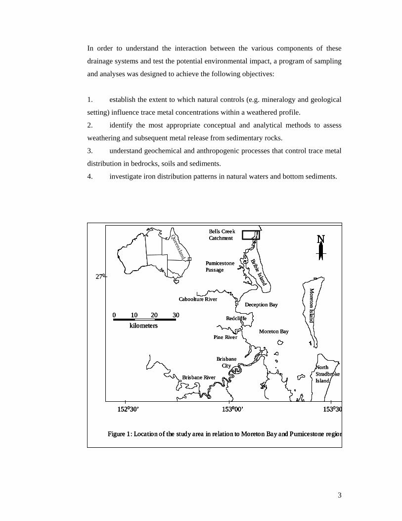
In order to understand the interaction between the various components of these

drainage systems and test the potential environmental impact, a program of sampling

and analyses was designed to achieve the following objectives:

1. establish the extent to which natural controls (e.g. mineralogy and geological

setting) influence trace metal concentrations within a weathered profile.

2. identify the most appropriate conceptual and analytical methods to assess

weathering and subsequent metal release from sedimentary rocks.

3. understand geochemical and anthropogenic processes that control trace metal

distribution in bedrocks, soils and sediments.

4. investigate iron distribution patterns in natural waters and bottom sediments.

270

Moreton Bay

Brisbane River

PumicestonePassage

Caboolture River

Pine River

0 10 20 30

kilometers

Bribie Island

Moreton Island

North Stradbroke Island

Redcliffe

153000’ 153030’152030’

BrisbaneCity

N

Deception Bay

Bells Creek Catchment

Figure 1: Location of the study area in relation to Moreton Bay and Pumicestone region.

Queensland

270

Moreton Bay

Brisbane River

PumicestonePassage

Caboolture River

Pine River

0 10 20 30

kilometers

Bribie Island

Moreton Island

North Stradbroke Island

Redcliffe

153000’ 153030’152030’

BrisbaneCity

N

Deception Bay

Bells Creek Catchment

Figure 1: Location of the study area in relation to Moreton Bay and Pumicestone region.

Queensland

Moreton Bay

Brisbane River

PumicestonePassage

Caboolture River

Pine River

0 10 20 30

kilometers

Bribie Island

Moreton Island

North Stradbroke Island

Redcliffe

153000’ 153030’152030’ 153000’ 153030’152030’

BrisbaneCity

NN

Deception Bay

Bells Creek Catchment

Figure 1: Location of the study area in relation to Moreton Bay and Pumicestone region.

Queensland

4

Figure 2: Aerial photo of the Bells Creek catchment with its land use practices

Glass House Mountains

Golden Beach

Pine Plantations

Bells Creek

Pumicestone Passage

Golf Course

Native Vegetation

5

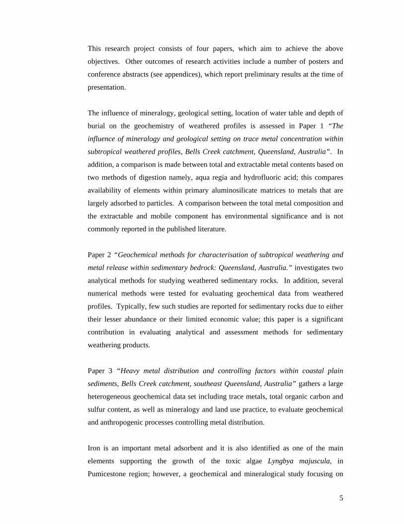
This research project consists of four papers, which aim to achieve the above

objectives. Other outcomes of research activities include a number of posters and

conference abstracts (see appendices), which report preliminary results at the time of

presentation.

The influence of mineralogy, geological setting, location of water table and depth of

burial on the geochemistry of weathered profiles is assessed in Paper 1 “The

influence of mineralogy and geological setting on trace metal concentration within

subtropical weathered profiles, Bells Creek catchment, Queensland, Australia”. In

addition, a comparison is made between total and extractable metal contents based on

two methods of digestion namely, aqua regia and hydrofluoric acid; this compares

availability of elements within primary aluminosilicate matrices to metals that are

largely adsorbed to particles. A comparison between the total metal composition and

the extractable and mobile component has environmental significance and is not

commonly reported in the published literature.

Paper 2 “Geochemical methods for characterisation of subtropical weathering and

metal release within sedimentary bedrock: Queensland, Australia.” investigates two

analytical methods for studying weathered sedimentary rocks. In addition, several

numerical methods were tested for evaluating geochemical data from weathered

profiles. Typically, few such studies are reported for sedimentary rocks due to either

their lesser abundance or their limited economic value; this paper is a significant

contribution in evaluating analytical and assessment methods for sedimentary

weathering products.

Paper 3 “Heavy metal distribution and controlling factors within coastal plain

sediments, Bells Creek catchment, southeast Queensland, Australia” gathers a large

heterogeneous geochemical data set including trace metals, total organic carbon and

sulfur content, as well as mineralogy and land use practice, to evaluate geochemical

and anthropogenic processes controlling metal distribution.

Iron is an important metal adsorbent and it is also identified as one of the main

elements supporting the growth of the toxic algae Lyngbya majuscula, in

Pumicestone region; however, a geochemical and mineralogical study focusing on

6

iron species and their source is lacking. Therefore, paper 4 “Distribution of Fe in

waters and bottom sediments of a small tidal catchment, Pumicestone Region,

southeast Queensland, Australia” aims to identify the source and establish the

process of iron transport through bottom sediments, surface, groundwater and by

suspended matter within Halls Creek sub-catchment.

In summary, the study of this subtropical catchment is designed to determine two

aspects: (a) the natural and anthropogenic factors controlling geochemistry of

weathered profiles, sediments, soils and natural waters of the area, and (b) identify

the best analytical and numerical methods for evaluating metal concentrations in

weathered profiles and large heterogeneous geochemical data sets.

References

CRANFIELD L.C. 1983. Shallow stratigraphic drilling in the Brisbane 1:100,000

Sheet area. Record 40, Geological Survey of Queensland.

EZZY T.R., COX M.E. and BROOKE B. 2002. The influence of stratigraphy on the

occurrence and composition of groundwater within a coastal valley-fill:

Meldale, south-eastern Queensland. In: HAIG T., KNAPTON A., GEORGE

D. and TICKELL S. (eds.). Balancing the groundwater budget, CD of

conference proceedings, International Association of Hydrogeologists

groundwater conference, 12-17 May, Darwin, Australia, pp. 6.

FAURE G. 1998. Principles and application of geochemistry, 2nd edition, Prentice

Hall, New Jersey, pp. 600.

FLOOD P.G. 1981. Carbon-14 dates from the coastal plains of Deception Bay,

south-eastern Queensland. Queensland Government Mining Journal, 82: 19-

23.

LESTER J. 2000. Geomorphology, sedimentology and shoreline processes impacting

on the stability of the Bribie Island Spit. Honours thesis, School of Natural

Resource Sciences, QUT.

MURPHY P.R., TREZISE D.L., HUTTON L.J. and CRANFIELD L.C. 1987.

1:100,000 Geological Map Commentary. Caboolture, Sheet 9443,

Queensland Department of Mines, Geological Survey of Queensland.

7

WILLIAMS M., DUNKERLEY D., DE DECKKER P., KERSHAW, P. and

CHAPPELL J. 1998. Quaternary environments. Arnold, Hodder Headline

Group, London.

8

LITERATURE REVIEW

9

A BACKGROUND TO GEOCHEMISTRY

Geochemistry is the application of the principles of chemistry to solve geological

problems. Geochemistry as defined by Goldschmidt and summarised by Mason

(1958, p. 2) is concerned with (1) the determination of the relative and absolute

abundance of elements in the earth, and (2) the study of distribution and migration of

the elements in the various parts of the earth to discover philosophies governing this

distribution and migration. In a more recent definition by Faure (1998), there are

four major goals in geochemistry:

• To understand the distribution of the chemical elements in the Earth and in the

solar system.

• To determine the origin of the observed chemical composition of terrestrial and

extraterrestrial materials.

• To study chemical reactions on the Earth, its interior and in the solar system.

• To congregate these findings into geochemical cycles and to explore their

operational systems in the past and how they may be altered in the future.

Mineral exploration is one of the oldest applications of geochemistry and is defined

as systematic measurement of one or more chemical properties of a naturally

occurring material to locate hidden ores (Hawkes and Webb, 1962). Environmental

geochemistry is a more recent form of geochemistry, which is focused on monitoring

the dispersion of metals and various organic compounds that have anthropogenic

sources. Since the middle of the 20th century, geochemistry has become diversified

into several subdivisions, among them inorganic and organic geochemistry,

cosmochemistry, isotope geochemistry, geochemical prospecting, medical

geochemistry, aqueous geochemistry and trace element geochemistry. This review

will present a summary of relevant literature on aqueous and trace metal

geochemistry.

Environmental geochemistry is of a great importance as it contributes to the

continued well being of human kind and assists in the development and management

of natural resources. The understanding of processes occurring on the Earth will

enable us to monitor the quality of the environment both locally and on a global

10

scale, and to warn humanity against dangerous practices that may threaten the quality

of life in the future (Faure, 1998).

On the basis of variables such as pressure, temperature and the availability of the

most abundant chemical component, it is possible to classify all the natural

environments of the earth into two major groups – primary and secondary (Hawkes

and Webb, 1962). The primary environment is characterised by high temperature

and pressure, restricted circulation of fluids and relatively low free oxygen content;

these conditions occur deep into the earth where most rocks form. The secondary

environment is of low temperatures, nearly constant low pressure, free movement of

solutions containing free oxygen, water and CO2. This latter environment is where

weathering, erosion and sedimentation at the surface of the earth take place.

One of the objectives of this study is to investigate the geochemical and

mineralogical composition of bedrock, soil and sediments of the study area; a brief

review on weathering therefore, is essential to explain the significance of a detailed

chemical and mineralogical analysis of the material throughout the field study area.

As the investigation also focuses on establishing occurrence and distribution of

heavy metals, it is important to understand the geochemical character of the

sedimentary environment. This understanding in turn will help to confirm the source

and distribution, adsorption and mobilisation of trace metals. Identifying and

understanding the geochemistry of post depositional processes associated with metal

occurrence in the Pumicestone Passage is another objective of the study; a brief

background about environmental geochemistry and geochemical cycles is also

presented. Trace elements in the sediments are a potential source of contamination

for surface and shallow groundwater; a summary of the environmental implications

of trace metal presence within such waters is therefore required. As the trace metal

geochemical dataset from coastal sediments produced in the current study is typically

heterogeneous, this review also discusses the approaches to assessment and analysis

of such datasets. There is no consensus about the most appropriate analytical

technique to determine trace metal contents in soils and sediments, therefore, a

variety of procedures have been assessed in the final part of this review.

11

The literature review outlines:

� Chemical weathering and environmental factors influencing it

� Products of chemical weathering

� Methodologies for assessing weathering profiles with regard to trace metals

� Sedimentary environments, their properties and geochemistry

� Trace metal occurrence and mobility

� Trace metals and water quality

� Analysis of heterogeneous geochemical datasets

� Comparability of analytical methods for environmental samples

WEATHERING OF THE BEDROCK

Introduction

Natural processes such as weathering and erosion of the land surface as well as

anthropogenic activities can result in a major input of heavy metals into the coastal

and estuarine environments. Iron, Mn, organic C and S act as metal scavengers in

transportation and deposition of trace elements into the sediments (e.g. Förstner and

Muller, 1973). Many metals occur naturally in weathered materials and drainage

systems due to their presence in local rocks; therefore, in order to understand

distribution and mobility of these elements on the earth surface, it is essential to

identify natural sources of metals and gain knowledge of weathering and associated

processes, which is explained below.

The upper 15 km of the lithosphere is comprised of 95% igneous rocks, 4% shales,

0.75% sandstones, and 0.25% limestones (Carroll, 1970). Only 30% of lithosphere is

dry land of which only the upper surface is affected by some degree of chemical

decomposition or physical weathering (Carroll, 1970). The weathering of rocks

composing the lithosphere occurs through chemical, physical and biological

processes. Details of these processes are not the focus of this review and can be

found in books about weathering and soil formation such as those by (Goldich, 1938;

Colman and Dethier, 1986; Lerman and Maybeck, 1988; Nahon, 1991; Berner and

Berner, 1996; Bland and Rolls, 1998).

12

As it is important to understand variations of major and trace elements related to

chemical and mineralogical changes during intense weathering in a subtropical

environment, products of, and factors controlling chemical weathering will be

discussed in more detail in the following sections.

Factors controlling chemical weathering

The nature of chemical weathering varies widely and is governed by many variables

such as parent rock type, topography, climate, time and vegetation. As the extent of

weathering is a controlling factor on trace metal distribution and mobilisation the

influence of mineralogy and geological setting on trace metal concentration within

weathered profiles has been investigated in the paper “The influence of mineralogy

and geological setting on trace metal concentration within subtropical weathered

profiles, Bells Creek catchment, Queensland, Australia” . The mobilisation and

redistribution of trace elements during weathering is particularly complex because

these elements are affected by various processes such as dissolution of primary

minerals, formation of secondary phases, redox processes, transport of materials,

coprecipitation and ion exchange (e.g. Nesbitt, 1979; Chesworth et al., 1981; Cramer

and Nesbitt, 1983).

PARENT MATERIAL

While the ultimate composition of weathered bedrock formed by near-surface

processes is related to the composition of the source rock, studies have shown that

both chemistry and mineralogy of the weathered profile may differ greatly from

those of the bedrock on which it forms. For example Boggs (1995) demonstrated

that the composition of weathered bedrock is controlled not only by the parent-rock

but also by the nature, intensity and duration of weathering and soil-forming

processes. Furthermore, where there are extreme differences between chemistry and

mineralogy of the weathered profiles and their parent material, in situ chemical

weathering has been accompanied by additional subtractions such as colluvial and /or

alluvial addition that contributed in weathering.

Variations in texture, structure and composition of bedrock can exert a significant

influence on the rate of leaching. Texture affects permeability and therefore, the

degree of penetration of rainwater into the rock. For instance, loose sands are

13

particularly permeable and the soluble constituents can readily leach from areas

above the water table. On the other hand, clayey soils tend to inhibit penetration of

water and increase the loss through surface runoff. In consolidated rocks, fractures

and zones of weakness such as joints, faults, and cleavage offer easy access to water

and accelerate the leaching process as well as providing channels for the subsurface

drainage. In addition, through the development of a mature weathered zone, the rate

of weathering may alter (Loughnan, 1969).

Profiles with different parent material also weather differently. Sedimentary rocks

weather more readily than igneous and metamorphic rocks due to hydrodynamic

processes. For chemical weathering to occur to a significant degree, water must

circulate through the rock. This is more conductive in open structure of sedimentary

rocks compared to most igneous and metamorphic rocks. There are some exceptions

such as the exclusive Carboniferous limestone of England and Wales that is resistant

to weathering (Macias and Chesworth, 1992). When sedimentary rocks are

compared, mudstone has been found to deteriorate to a larger extent compared to

sandstone because the large amount of Fe in both sedimentary rocks behaves

differently. While sandstone is strengthened because of cementation by iron oxides

or hydroxides, mudstone is weakened because it contains a greater amount of clay

size fractions with larger specific surface area than sandstone (Chigira and Sone,

1991; Chigira and Oyama, 1999). Different types of rocks have different mineralogy

and thus chemical character, therefore, influencing the local weathering environment

as they breakdown. For instance, the feldspars in a granite weather to produce a

solution containing K+, Na+, Ca2+, consuming hydrogen ions in the process, thus the

weathering solution becomes more alkaline. Sulfide minerals however, weather by

oxidation, converting the sulfur to sulfuric acid with a marked increase in acidity of

the water (Taylor and Eggleton, 2001).

In areas with homogeneous climates, where sedimentary covering is sparse and

lithological variability pronounced, parent rock has a significant role on weathering.

However, in an edaphological zone (the unconsolidated mineral material on the

immediate surface of the earth that serves as a natural medium for the growth of land

plants) with a relatively homogeneous bedrock type, the parent rock effect can be

masked by the effect of climate and vegetation (Macias and Chesworth, 1992).

14

TOPOGRAPHY

Topography affects the rate of chemical weathering and the nature of the weathered

products by controlling: 1) the rate of surface runoff of rain water and therefore, the

rate of moisture intake by the parent rock, 2) the rate of subsurface drainage and

hence the rate of leaching of the soluble constituents, and 3) the rate of erosion of the

weathered products and thereby the rate of exposure of fresh mineral surfaces.

On very steep slopes most of the rainwater is lost due to surface runoff and at the

same time physical weathering occurs by running water, wind and landslides.

Hence, in such environments, physical disintegration of rocks proceeds at a much

greater rate than chemical breakdown and any accumulation of secondary minerals is

superficial. In low-lying lands such as coastal plains, surface runoff is minimal and

infiltration of rainwater is at a maximum rate. In this type of environment subsurface

drainage is sluggish and soluble products released by hydrolysing reactions are

preserved, thus preventing further breakdown of parent material. The ideal condition

for chemical weathering is attained on gently sloping uplands where surface runoff is

not excessive and the subsurface drainage is unrestrained. Under such condition, the

weathered zone may extend to a depth of 30 m or more (e.g. Jenny, 1941; Loughnan,

1969; Taylor and Eggleton, 2001). Thus, although landscape position is important,

the degree of importance depends on drainage characteristics.

Groundwater movement is another aspect related to weathering. It is the movement

of shallow groundwater that transports solutes from higher parts of the landscape to

lower enabling weathering reactions to continue. In addition, solid particles may be

moved downwards through the weathering material, depositing deeper in the profile.

Fine-grained particles such as clays and Fe-oxides are most easily removed (leached

or eluviated). Landscape shape also has a considerable effect on the groundwater

movement patterns. While under long straight slopes groundwater contributes to the

stream uniformly along the valley, at the valley heads the groundwater flow is

concentrated and tends to intensify solution movement, weathering and erosion by

mass movement. At spurs, groundwater will deliver less solutes and erosion by mass

movement will be less. This means that due to the higher groundwater flows in

valley heads, weathering rates are likely to be higher in such areas compared to

15

anywhere else in the catchment (Taylor and Eggleton, 2001). The role of mineralogy

and that of geological setting on the trace metal concentrations in weathered profiles

has been investigated in the paper “The influence of mineralogy and geological

setting on trace metal concentration within subtropical weathered profiles, Bells

Creek catchment, Queensland, Australia”. A comparison is made between the total

metal composition and the extractable and mobile component which has

environmental significance but is rarely presented in published literature.

CLIMATE

Climate is a paramount factor in chemical weathering as it controls the amount of

rainfall for an environment (Summerfield, 1991). Rainfall in particular, controls the

supply of moisture for chemical reactions and the removal of soluble constituents of

the minerals. Temperature has also considerable influence on the rate and intensity

of chemical weathering. According to the “van’t Hoff’s rule”, for each 10º C rise in

the temperature the velocity of a chemical reaction increases by a factor from 2 to 3

(Taylor and Eggleton, 2001). It is mainly the proportion of the total rainfall which

infiltrates the weathering zone, percolates downward and ultimately finds its way by

subsurface drainage to creeks, rivers, lakes and the ocean, carrying dissolved

constituents that governs the rate of weathering.

In arid regions where evaporation exceeds rainfall, water may penetrate the rocks but

during long dry periods, it is lost through evaporation. Therefore, soluble

constituents of the rocks are not removed and reactions are slowed down. Such areas

are characterised by unaltered or partly altered parent minerals, the presence of salts

such as gypsum and carbonates, alkaline pH values (7.5-9.5), and a general scarcity

of organic matter. The characteristic secondary minerals are montmorillonite, illite,

chlorite and mixed layers of these minerals. In contrast, the rocks of humid areas are

generally well leached due to continual downward movement of the percolating

waters and the soluble products of the hydrolysing reactions ultimately lost through

subsurface drainage. Under these conditions chemical weathering proceeds rapidly

and the most abundant secondary minerals are kaolinite, halloysite and gibbsite as

well as ferric oxide minerals such as hematite and goethite (Crowther, 1930;

Loughnan, 1969). Of note is that a change in temperature does not, however, affect

the processes of weathering. If a rock is so placed that it weathers to bauxite in the

16

tropics, the same rock in the same regolith situation but in Iceland, may also weather

to bauxite, but it will take substantially longer (Taylor and Eggleton, 2001).

TIME

Time can be considered a geological factor. While the effects of weathering can

produce rudimentary soils within times of the order of hundred or several hundred

years, it takes millions of years to produce a ferrasol. Furthermore, in humid climatic

zones, the effect of parent material becomes more difficult to detect as reaction time

increases. On any time-scale, especially on geological ones, there is always a

significant lag between the establishment of a particular set of conditions in the

weathering environment and the adjustment of the mineralogical and physical

properties of the regolith to these conditions. Therefore, weathering profiles are

rarely in full equilibrium with environmental conditions as these conditions

constantly change; in most cases the weathering mantle adjusts to long-term average

conditions rather than to conditions at a specific time (Summerfield, 1991; Macias

and Chesworth, 1992).

VEGETATION

Vegetation directly affects weathering through the release of organic acids and in the

supply of carbon dioxide to soil waters. This occurs by the production of litter which

varies substantially not only between deserts and forest ecosystems but also between

temperate forest with a typical range of 0.1-0.3 × 106 kg/ km2/year and tropical

rainforests which produce 0.4-1.3 × 106 kg/ km2/year (Summerfield, 1991). Organic

activity is closely related to climatic controls, but vegetation type also varies by

topographic factors and soils properties. Therefore, it can indirectly influence

weathering through topography (Summerfield, 1991).

Products of Chemical Weathering

During chemical weathering (dissolution, oxidation, hydrolysis, acidolysis or

alcalinolysis) decomposition of primary minerals leads to the formation of secondary

minerals. Rock-forming minerals are partly dissolved during the weathering process

and hydrolysis and hydration take place. Clay minerals are the most significant type

of secondary minerals due to their complex phyllosilicate properties (e.g. surface

area and internal structure). These characteristics make them metal adsorbents (e.g.

17

Berner, 1971; Chamley, 1989; Summerfield, 1991; Velde, 1992; Hamblin and

Christiansen, 2001) and could be significant for the depositional environment as they

may act as geochemical traps for heavy metals. Furthermore, clay minerals such as

mixed layers of smectite-illite are the species that are likely to be encountered in the

subtropical setting of this project study area (Cox et al., 2000). Therefore, a brief

discussion about clay minerals with special regard to their speciation, distribution

and depositional significance is presented in this review.

Clay Minerals

While clay minerals occur in a variety of forms, only the major groups are discussed

here. Recombination of silica, aluminium and metal cations released during

weathering can form layered phyllosilicate structures. The type of clay minerals

produced in the sedimentary environment depends on the composition of the

circulating pore waters, the mineralogy of primary materials, the intensity of leaching

and the prevailing Eh-pH conditions (Chamley, 1989; Summerfield, 1991).

Under intense leaching conditions, kaolinite is prevalent. Conditions of extreme

leaching can ultimately lead to the formation of iron (goethite) and aluminium-rich

oxides (gibbsite). If leaching is only moderate however, the formation of cation-

bearing clays such as illite and smectite are favoured. Therefore, in a sedimentary

setting the magnitude of the weathering can be predicted from the type of the most

prevalent clay mineral present.

Clay minerals are stable under conditions of normal pressure and temperature; clays

therefore, experience only limited mineralogical transformation during transport and

after deposition in the marine environment. As a result, they are an excellent tracer

for sediment origin, distribution and transport pathways over long distances, as fine-

grained sediments of different origin can often be differentiated by their clay mineral

content (Zollmer and Irion, 1993; Algan et al., 1994). While in this study the clay

speciation is homogeneous throughout the catchment due to the existence of a

relatively uniform bedrock (Landsborough Sandstone), it may have a depositional

significance. Due to limited leaching and physical rework, it is expected that the

fluvial material (upstream) may contain more smectite. In addition, smectite may be

deposited in lower energy sections of the estuarine section and around meanders. In

18

most downstream settings, however, smectite has been weathered to kaolinite (e.g.

Chamley, 1989; Velde, 1992).

While a detailed review of weathering processes is not the focus of this study, a brief

discussion about the mechanism/s involved in silicate weathering and secondary

mineral formation is of significance, as it helps to understand the depositional

significance of clay minerals throughout the study area. When weathering occurs, a

primary mineral (e.g. silicate or carbonate) is attacked by organic acids such as

oxalic acid. However, the overall reaction, as far as groundwater composition is

concerned, can be presented as if the only attacking acid was H2CO3. In other words,

HCO3- and not C2O4

2- is found in most groundwater and river waters (Berner and

Berner, 1996 for detailed reactions between silicates and organic acids). Thus, as

organic acids disappear soon after primary mineral attacking, it is the general

assumption that silicate weathering consists solely of attack by carbonic and sulfuric

acids (e.g. Garrels, 1967). This is a simplification of a series of more complex

chemical weathering reactions which enables the prediction of the origin of ions in

groundwater without concern for the type of organic acid attacking the primary

minerals. As weathering proceeds, aluminium liberated by feldspar dissolution

precipitates to form a secondary clay mineral, except for localised distribution

accompanying chelate transport. Iron, due to its insolubility in the presence of O2,

also accumulates in soils, as ferric oxides.

Precipitation of Al may form gibbsite, smectite or kaolinite under different

conditions. Concentrations of these secondary minerals build up during contact of

the water with primary minerals, however, when the water leaves the rocks, further

build-up will cease. The faster the rock is flushed with water, the shorter will be the

time of contact with the primary mineral, and the higher will be the intensity of the

weathering of the rock. Gibbsite formation represents a high degree of flushing with

removal of both cations and silica. Kaolinite represents less rapid flushing with less

removal of silica, and smectite occurs under stagnant conditions of water flow so that

appreciable build-up of both silica and cations can take place (Berner and Berner,

1996). The following are the chemical reactions occurring in silicate weathering

(Thomas, 1994):

19

The first step is the hydrolysis of albite:

2NaAlSi3O8+3H2O+CO2 → Al2Si2O5(OH)4 + 4SiO2 + 2Na+ + 2HCO3-

albite kaolinite ions in solution

The highly mobile Na+ ion is lost in solution along with some proportion of the silica

which is not recombined to form clay minerals (kaolinite). The silica not combined

as kaolinite goes into solution as silicic acid:

SiO2 + H2O → 4Si(OH)4 (or H4SiO4)

silica silicic acid

Under weakly acid conditions with sufficient water and free drainage, more silica

may be removed, allowing gibbsite to form from kaolinite (incongruent dissolution

of Al and Si):

2Al2Si2O5(OH)4 + 105H2O → 42Al(OH)3 + 42Si(OH)4

kaolinite gibbsite

While gibbsite forms more commonly from the breakdown of kaolinite, it can also

form directly from plagioclase feldspar.

In conditions where water is scarce, the hydrolysis reactions may be retarded and

intermediate clay products will be formed:

8NaAl2Si3O8 +6H+ + 28H2O → 3Na0.66Al2.66Si3.33O10(OH)2 + 14H4SiO4 + 6Na+

albite smectite

or possibly

6KAlSi3O8 + 4H2O+ 4CO2 → 4K+ + K2Al4(Si6Al2O20)(OH4) + 4HCO3- + 12SiO2

illite

These clay minerals are more complex than kaolinite and their physical structure

reflects this complexity (Thomas, 1992).

In general, gibbsite forms in mountainous terrain with high rainfall and good

drainage where there is very rapid flushing. Tropical and subtropical soils tend to

favour formation of kaolinite due to less strong flushing. Finally, smectite is the

characteristic mineral of soils of semiarid regions with low rainfall. The effect of

flushing by water on the weathering of a single rock type is demonstrated by the

studies of Sherman (1952) (correlation between rainfall and clay assemblage) and

Mohr and van Baren (1954) (effect of drainage on clay mineralogy). Mohr and van

20

Baren found that for the same rock type and rainfall, depending on degree of

drainage, soils might have different clay mineralogy. While kaolinite is formed

under a good drainage system, in swampy depressions with poor drainage smectite

was more abundant. Furthermore, differences in water flow path could result in the

formation of different clay assemblages from the same plagioclase-rich rock under

the same climate and relief. In surficial zones where the water residence time was

short due to a small flow path gibbsite was formed. However, at depth both gibbsite

and kaolinite were found where the water travel distance was much greater. In the

slightly weathered and deeply buried underlying rock, the entrapment of water

resulted in the formation of smectite (Velbel, 1984).

Iron Minerals

The common iron minerals forming under sedimentary conditions include hematite,

goethite, siderite, glauconite and pyrite. Hematite and goethite are the oxidation

products of weathering of ferrous minerals and constitute a major source of detrital

iron in sediments. By contrast, glauconite, siderite and the iron sulfides form only

during diagenesis. Fine-grained goethite, FeOOH, is formed by the hydrolysis of

Fe3+ ions released during the oxidation and weathering of Fe-containing phases such

as limonite (e.g. Evans, 1989). While limonite is abundant in modern sediments and

on weathered outcrops, it is rare in buried ancient sedimentary rocks (Fischer, 1963),

and it is an assumption that it is unstable during diagenesis. Hematite however, is a

common mineral of sedimentary rocks and it is believed that if limonite disappears

during diagenesis some of it may be dehydrated to hematite. In order for this to

happen, the original sediment would have to be relatively free of decomposable

organic matter so a high enough Eh can be maintained to stabilise hematite.

Therefore, as organic matter is generally abundant in marine sediments, almost all

hematites are non-marine (Berner, 1971).

Thermodynamical stability of siderite (FeCO3) is severely restricted, as for the stable

form to persist Eh and S2- must be low. This is unlikely to occur in marine

conditions because low Eh is the result of the anaerobic bacterial decomposition of

organic matter; in seawater, which contains abundant dissolved sulfate, anaerobic

decomposition almost always includes the reduction of sulfate to H2S. Thus, if

thermodynamically reversible redox equilibrium between SO4aq2- and HSaq

-, or H2Saq,

21

is only obtained by sulfate reduction, then siderite has no stability field in marine

sediments. By contrast, in both ancient and modern non-marine sediments siderite

occurs commonly in association with coal beds and fresh-water clays (Berner, 1971).

Overall, iron minerals such as hematite and siderite are representative of a non-

marine sedimentary environment, as the marine conditions do not allow for the stable

form of these minerals to persist.

In waterlogged and saline sediments with a significant supply of decomposed organic

matter, bacteria break down this organic matter under anaerobic conditions, reducing

sulfate (SO42-) from seawater to sulfide. The iron source is from detrital ferric (Fe3+)

phases occurring as concretions, coatings or adsorbed by clay minerals oxidising to

Fe2+. The stable end product is pyrite (e.g. Berner, 1971, 1981, 1983; Dent, 1986;

Dent and Pons, 1995). Sea-level changes therefore, can influence pyrite formation;

over the last 6000 years for example, the Holocene sedimentation has kept pace with

sea-level fluctuations and has formed a broad, stable tide-influenced zone. This type

of setting has provided the required conditions for iron sulfide accumulation on many

of the world’s coastal plains (Dent, 1986).

Overall, three environmental systems for accumulation of pyrite have been identified

(Pons et al., 1982). System (1) includes bare tidal flats, marshes with mangrove

swamps in association with tidal creeks. The lower reaches of the system are

inundated most of the time and sediments are reduced; the higher reaches however,

have a predominantly aerated surface soil. In tropical regions, organic carbon

content of the sediments in this system is low (0.15 to 2%) but the system receives a

very high supply of organic matter from mangroves. Tidal flushing kinetically

favours pyrite formation in this system by supplying limited amounts of dissolved

oxygen necessary for complete pyritisation of reduced sulfate. Tidal flushing can

also enhance removal of sedimentary carbonate or bicarbonate from the system,

increasing the potential acidity of the system. This system is the most likely

environment occurring in the southern part of the study area (Halls Creek

catchment), most of which is a tidal-dominated floodplain accumulating large

amounts of pyrite compared with a fluvial-dominated area (e.g. Lin et al., 1995).

22

System (2), which occurs at the bottom of saline and brackish lagoons, seas and

saline lakes, always contains clastic sediments supplied by rivers. In arctic regions

this system comprises high amounts of organic material. However, where decay of

organic matter is slow, accumulation of sulfate can be considerable.

System (3) consists of poorly drained inland valleys with an influx of sulfate-rich

water. This system is very rare; examples are the pyritic papyrus in a few valleys in

the eastern Netherlands and the sulfidic peat soils of Minnesota, USA.

METHODOLOGIES FOR ASSESSING WEATHERING PROFILES WIT H REGARD TO TRACE METALS A substantial volume of literature is available on methodologies on assessing

weathering of volcanic or igneous rocks (e.g. Chesworth et al., 1981; Middelburg et

al., 1988b; Nesbitt and Wilson, 1992; Hill et al., 2000), however, similar

methodologies for sedimentary rocks are scarce. Therefore, the following are some

methods for evaluating geochemical data from weathered profiles that can be applied

to sedimentary rocks.

Calculation of Chemical and Mineralogical Indices

The chemical behaviour of minor and trace elements for a weathered profile and its

equivalent weathered products as a function of a mineralogical index of alteration

(MIA), rather than depth of sampling is one way of evaluating geochemical data.

Understanding the geochemical behaviour within the weathered profile therefore,

helps to explain the processes involved in mobilisation and deposition of these

metals in unconsolidated sediments throughout the catchment. The degree of

weathering varies for different samples at a similar depth, but in different cores can

be quantitatively measured, using the whole-rock analyses. These values represent

the average weathering index for each sample and can also be used to determine the

weathering index of each separate mineralogical component of the system. The main

assumptions are that the index of alteration of a sample is the same for all its

mineralogical pairs used for the partition of a chemical element between a primary

and its equivalent secondary mineral, and that the system is closed, without mass

transfer (loss or gain) (Voicu et al., 1996, 1997). The first step is to calculate the

23

Chemical Index of Alteration (CIA: Nesbitt and Young, 1982; Fedo et al., 1995) for

each analysed sample using the following equation:

CIA = [Al 2O3 / (Al2O3 + CaO + Na2O + K2O)] × 100 (1)

where oxides are in molecular proportions. While CIA was widely used as a

chemical index to ascertain the degree of source-area weathering (e.g. Bauluz et al.,

2000), according to Voicu and Bardoux (2002), CIA values range between 50 and

100 and cannot be directly applied for the normative calculations. Therefore, they

proposed a second step, the calculation of the mineralogical index of alteration

(MIA), using the following equation (Voicu et al., 1996, 1997):

MIA = 2 × (CIA – 50) (2)

The mineralogical index of alteration indicates the degree of weathering for each

analysed sample, independently of the depth of sampling. The MIA value indicates

incipient (0-20%), weak (20-40%), moderate (40-60%), and intense to extreme (60-

100%) weathering. The value of 100% means complete weathering of a primary

mineral into its equivalent weathered product (Voicu and Bardoux, 2002).

Therefore, the use of a weathering index such as MIA enables the quantification of

the supergene alteration of each individual sample and complements qualitative

estimation of weathering intensity by mineralogical studies such as x-ray diffraction

(XRD). Furthermore, it provides more accurate information about the trends of

major and trace element in weathered material as a comparison to unweathered

parent material.

Mass Balance Calculations

For an accurate assessment of element mobility during weathering, it is necessary to

look at absolute changes in element concentrations. This has been done using two

principal methods. The weight loss factor method (Faure, 1998) is based on the

assumption that during weathering, one of the major-element oxides has remained

constant in amount, although its concentration may appear to have changed. This

procedure is applicable during original transformation of parent rock to weathered

material where original mineral structure is maintained. The constituent chosen most

often for this purpose is Al2O3, which is generally immobile and remains in the

system (e.g. Faure, 1998). Alternatively, Fe2O3 (e.g. Faure, 1998), TiO2 (e.g.

24

Nesbitt, 1979; Eggleton et al., 1987; Hill et al., 2000), or ZrO2 (e.g. Hodson, 2002;

Steyrer and Strum, 2002) may be selected in the cases where Al is not the most

constant oxide.

In more severely weathered profiles however, the original structures and volume are

not preserved and the immobile element approach (Nesbitt, 1979) must be used to

assess element mobility. The percentage increase or decrease of any component (X)

in a weathered rock, relative to the fresh parent rock is calculated according to the

following equation:

Percentage change = [(X / I) weathered / (X / I) parent – 1] × 100 (3)

where I is the concentration of immobile component. In mass balance calculations,

losses are indicated by high (70-100%), average (40-70%) and low (0-40%) and

gains are shown by low / average (40-100%) and high (>100%) (Braun et al., 1993).

The paper “Geochemical methods for characterisation of subtropical weathering

and metal release within sedimentary bedrock: Queensland, Australia” presents the

applicability of the described procedures (chemical and mineralogical indices, weight

loss factor and immobile element) to the sandstones and mudstones present in the

study area.

25

SEDIMENTARY ENVIRONMENTS, THEIR PROPERTIES AND GEOCHEMISTRY

Introduction

Transported aquatic solids comprise a mixture of material inputs from different

sources. These can include eroded rocks and soils, solid waste particles, atmospheric

fallout and autochthonous formations such as inorganic precipitates, biogenic matter,

adsorbents on particles from solution, and other complexed and colloidal matter.

During periods of reduced flow rates, suspended material settles to the bed of the

river, lake or sea and incorporates into the bottom sediments (e.g. Förstner, 1983).

In detecting trace metal pollution sources, it is very important to study and analyse

sedimentary environments. Their significance was highlighted by Förstner (1983)

who stated that sediments with their contaminants have a relationship with the liquid

phases and the organisms; this means that the sediments themselves represent

another environmental contaminant. Sediment analysis has been significant in

identifying sources of trace metals in the aquatic environment for two main reasons:

(1) they exhibit higher accumulation rate (Förstner, 1981) and (2) sediment analysis

allows contaminants that are adsorbed by particulate matter, and thus escaping

detection by water analyses, to be identified (Förstner and Salomons, 1980).

Förstner and Salomons (1980), summarised important problem areas with regard to

the presence of contaminated sediment in the environment as follows:

• contaminants in the sediments are potentially available for aquatic life;

• contaminants in dredged material during and after disposal in dumping area could

cause groundwater pollution;

• vegetation may uptake contaminants from polluted sediments.

To assess the environmental impact of contaminated sediments, vertical sediment

profiles (cores and cuttings) are of importance. This is because the sedimentary

material often preserves the historical sequence of pollution, and at the same time

enables a reasonable estimation of the background levels and the variations in input

of pollutant over an extended period of time. It has been established that vertical

26

sections of the sediment could give a record of level of contamination over time, if

the pollutants are persistent and the sediment stratum has not seriously disturbed by

human activities such as clearing and dredging (Fung, 1993).

Overall, there are two primary aims for environmental studies of sediments: (1) to

identify, monitor and control pollution sources, and (2) to estimate possible effects of

polluted sediments. The results of sediment studies may vary due to sampling

techniques, preparation of samples and analytical procedures. In addition, sediment

metal concentrations are also influenced by sediment properties, for example pH,

redox potential, cation exchange capacity, soil texture and organic content (Ong Che,

1999). Therefore, the above limitations should be considered in making any

conclusions and/or generalisations.

As part of this study is focused on the effect of sediment grain size (mineralogy) on

trace metal chemical behaviour and the resultant geochemistry of estuarine

environments, these will be addressed in the next sections.

Properties of Sedimentary Material

Knowledge of the various characteristics of sediment (e.g. sediment size and

composition with respect to adsorbent material) enables assessment of its character

and evolution. A wide granulometric range, abundant matrix, poor sorting, angular

grains as well as high porosity and permeability characterize immature sediment.

Such sediment is the result of rough hydrodynamic actions, slow or weak, as

encountered in certain fluvial or glacial environments and during marine re-

sedimentation. However, mature sediment is evidence for active and prolonged

hydrodynamic processes in water or air, such as in littoral or desert dunes, beaches,

and other shallow-marine exposed environments (Chamley, 1989).

Sedimentary materials range from the fine dust transported by high-altitude winds to

large erratic blocks moved by glaciers. Sediments transported by and depositing

from waters tend to be within the smaller grain size range. Sedimentary particles

mostly fall in three categories, sand (2-0.063 mm), silt (0.063-0.004 mm), and clay

(below 0.004 mm) (Chamley, 1989). It has been established that the fine fraction of

sediment (<63 µm) has high concentration of heavy metals due to the strong

27

adsorptive surface properties of clay minerals and increased specific surface area

(e.g. Förstner and Salomons 1980; Förstner et al., 1982). This finding has also been

confirmed by other studies (Ellaway et al., 1982; Yocesoy and Ergin, 1992; Irvine

and Birch, 1998; Birch and Taylor, 1999). In a study of the influence of sediment

grain size on the metal concentration, Ellaway et al., (1982) separated samples into

three size fractions (clay < 2 µm, fine silt 2-20 µm, and coarse silt 20-63 µm) slightly

different from categories mentioned earlier, although the influence over metal

adsorption is similar.

Overall, there is some disagreement about the best size fraction to consider as an

indication of trace metal contamination. In the current study, the samples were not

sieved and chemically analysed according to their size, because any sieving may

contaminate the sediments. The effect of the fine-grained fraction on trace metal

content was investigated by determining the mineral composition using x-ray

diffraction analysis, which provides a more precise evaluation of the metal adsorbent

phases. The composition of sediments (see trace metal mobility) with respect to

adsorbent components is also related to the size of sediments because of the potential

influence on mobility of trace metals.

Geochemistry of Sedimentary Settings

An understanding of the geochemical settings of the sedimentary environments

enables the determination of how elements interact and associate with each other.

Consequently, this information can provide an understanding of the distribution of

metals, occurrence and availability to the overall system. Based on the early work of

Krumbien and Garrels (1952), the geochemical environment of sedimentary rocks is

characterised in terms of pH and Eh. However, in more recent studies, the

classification scheme of Berner (1981) is used. In this classification, in order to

determine the relevant environment of sedimentary rocks, the presence or absence of

total dissolved oxygen and sulfide phases (H2S and HS-) are considered. This

scheme is used because aerobic organisms and oxidised minerals cannot tolerate

traces of H2S without death or conversion to sulfide minerals, respectively.

Moreover, sulfide minerals and bacteria that produce H2S in sediments cannot

tolerate traces of oxygen without conversion to oxidised minerals or death. This

simply means H2S and oxygen cannot co-exist in solution (Berner, 1981).

28

Based on the above classification there are two major geochemical categories for

sedimentary environments in this scheme. They are known as oxic and anoxic,

depending on the presence and absence of oxygen, respectively (Berner, 1981). The

implication of anoxic and oxic sedimentary environments with respect to metal

occurrence is that firstly, under reducing conditions (anoxic) trace metals tend to be

less mobile and secondly, pyrite forms under reducing conditions and incorporates

heavy metals if available. Oxidation (oxic) conditions, however, will produce

sulfates, iron, acid and trace metals.

Coastal Marine Sedimentary Environments

There are several types of marine sedimentary environment including deltas and

estuaries, littoral, and shelf settings. As the focus of this project is on an estuarine

setting, they will be explained in more details as follows.

Depending on the approach taken, there are several ways to define estuaries. Based

on Dyer’s (1997) definition estuaries are formed at the mouth of rivers and in the

narrow boundary zone between the sea and the land. Their form and extent is

continuously altered by the erosion and deposition of sediment. A small rising or

lowering of sea level may have drastic effect on estuaries.

A typical estuary represents part of a river under the influence of tides. Although the

salt/freshwater interface is continuously changed, the salinity decreases in the

upstream direction. Therefore, in such environments, marine influences and

especially tidal processes are of significance. For example, deltas and estuaries

represent a continuous series of sedimentary environments at the interface of alluvial

plains and basins where fluvial processes interact with the influences of tides and

waves. An estuary denotes an extreme type of a delta subjected to tidal influences

and if at any stage of its evolution, it is dominated by fluvial supply, it tends to

become a seaward-advancing delta (Chamley, 1989).

While most oceanographers, engineers and natural scientists define estuaries as areas

of interaction between fresh and salt water, there are over 40 different definitions of

29

estuaries (Perillo, 1995). Some consider both tide effects and sediment point of view

(e.g. Chamley, 1989; Dyer, 1997) and some may consider only one of the above.

Pyrite-bearing sediments are typical of estuarine settings and known to be a potential

source of metals to both surface and groundwater. Main metals involved are

aluminium and iron, and therefore, their formation and release to the environment are

discussed in the following section.

Pyritic Sediments and Trace Metals

BACKGROUND AND DEFINITION

The accumulation of pyrite in low-lying coastal sediments is the first step in the

formation of acid sulfate soils (ASS), which is the most common form of acid soils

worldwide. Such soils have been divided into actual acid sulfate soils (AASS), and

potential acid sulfate soils (PASS) (Dent and Pons, 1993). It has been estimated that

AASS cover approximately 12 million ha of land around the world whereas PASS

cover more than 100 million ha (Dent, 1986).

Formation of ASS can be divided into accumulation of pyrite particles and oxidation

of pyrite sediments. The most essential factors involved in pyrite accumulation are:

sufficient amount of Fe3+, decomposed organic matter and sulfate ions under

anaerobic conditions. In different sediments, formation of pyrite is governed by

different factors. For example, in terrigenous marine sediments, mainly organic

matter controls pyrite whereas in non-marine, freshwater sediments accumulation of

pyrite is controlled by concentration of sulfate rather than organic matter (Berner,

1983).

Exposure of pyritic sediments can release acid, which in turn produces iron from

pyrite and aluminium from silicates to the ground and surface waters resulting in

significant acidification (Sammut et al., 1996). Trace metals can also be released,

mobilised and adsorbed to the surface of iron and manganese oxides and hydroxides,

by clays, or complex with organic compounds. The products resulting from

disturbance of pyritic sediments have detrimental environmental impacts in several

ways: (a) sulfuric acid can have an adverse impact on land and aquatic habitats, (b)

elements contained by pyrite are released and mobilised into the environment, and

30

(c) the weathering of pyritic sediments is enhanced by acidic condition, which results

in releasing major and minor metals from silicate structures and trace metals from

minerals (Preda and Cox, 2001). In Australia, major soil acidification has been

reported in Holocene estuarine sediments of coastal flood plains and modification of

these flood plains has accelerated the production and transport of acidified water

(Sammut et al., 1995).

FORMATION AND MORPHOLOGY

Framboids of pyrite are the most common texture of sulfides. They are present in

different environments, from recent sediments (marine and lacustrine) to sedimentary

and metamorphic, to magmatic rocks and hydrothermal deposits. However, their

most typical environment is represented by organic rich marine sediments

(Sawlowicz, 2000). Pyrite framboids are common below the sediment – water

interface (Canfield et al., 1996; Wilkin and Barnes, 1997a, 1997b; Suits and Wilkin,

1998), but are rarely found in the water column (e.g. Skei, 1988; Lyons, 1997).

While the framboids precipitate by gravitational force to form a geopetal fabric

inside the pores of sediment (Kawamura et al., 2002), Ski (1988) demonstrated the

presence and the formation of suspended framboidal pyrite in the highly anoxic

waters of Framvaren Fjord. Other workers have found suspended framboids in water

columns and due to oxic conditions concluded that pyrite was either resuspended or

has been transported from elsewhere. This may be due to the fact that estuarine

water does not contain enough oxygen to rapidly oxidise suspended pyrite framboids,

or alternatively organic inhibitors and surface coatings prevent rapid oxidation (e.g.

Middelburg et al., 1988a).

The morphology of the framboids varies from spherical to euhedral with the latter

more common in large particles. It has been demonstrated that the morphology of

pyrite crystals formed at room temperature is primarily controlled by the degree of

supersaturation in the solution from which pyrite is precipitated (Murowchick and

Barnes, 1987). With the increasing supersaturation, pyrite morphology changes from

cube to (euhedral) octahedron, to spherule (Wang and Morse, 1996). Therefore,

observed pyrite octahedra modified by cubes suggest a decrease in supersaturation

during crystal growth (Bulter and Rickard, 2000). Close spatial association of pyrite

framboids and euhedra in nature may be related to their genetic relationship. The

31

possibility of recrystalisation from framboidal to single grain pyrite has been

suggested (Love and Amstutz, 1966). Sawlowicz (2000) developed this idea and

proposed a continuous growth of microcrystals in the framboids (sometimes towards

euhedra) as long as they are in contact with the initial solution. While pyrite in any

morphological form or size is a major scavenger for chalcophile trace elements in

sedimentary environments, in its framboid form due to its much larger surface area

can accumulate more metals compared to its euhedral form. The spatial

morphological variation of pyrite was investigated in the paper “Distribution of Fe in

waters and bottom sediments of a small tidal catchment, Pumicestone Region,

southeast Queensland, Australia”.

TRACE METALS Occurrence

In sedimentary environments metals may occur as (a) adsorbed on solids, (b)

precipitated and coprecipitated on solids (Fe and Mn as metallic coatings), (c)

incorporated in solid biologic materials, and (d) incorporated in crystal structures

(Förstner and Wittman, 1983). Metals occurrence in rock forming minerals is based

on the type of crystallographic structure, for example, while quartz and alkali-

feldspar have low concentrations of heavy meals, magmatic minerals (biotite,

pyroxene and olivine) contain higher levels of heavy metals.

A major input of various metals to coastal lowlands may occur as a result of

weathering and erosion of geological formations. These trace metals are transported

from their source as either dissolved or particulate forms by streams and rivers and

are deposited on coastal floodplains, and in estuaries and bays. In such aquatic

environments, metals undergo various processes associated with floods, tides, and

waves and can be adsorbed by clays, complex with organic compounds or co-

precipitate as inorganic mineral phases. Human activities are a major source of

introducing trace metals into coastal environments. Hence, in estimating total metal

composition in such settings, both natural regional abundance and local

anthropogenic inputs have to be considered (Preda and Cox, 2001, 2002).

Trace metals therefore, may be introduced to the coastal environment by both natural

processes (e.g. weathering and erosion) and human activities in catchment area or

32

adjacent to the coast (Niencheski et al., 1994; Preda and Cox, 2001). These studies

further explained that in transfer from water to sediment, metal may involve co-

precipitation and adsorption on freshly precipitated Fe/Mn hydroxides and adsorption

on clay minerals and organic matter. Ong Che (1999) showed that metal

concentration in the surface sediments were 4-25% higher than those found in the

deeper sediments, reflecting anthropogenic input to the sediment metal load.

Niencheski et al., (1994) suggested that in assessing metal contamination in coastal

areas, studies of water column concentrations of trace metals are difficult because of

the possibility of sample contamination during collection and handling and

requirements for ultra-trace analysis. Therefore, they concluded that as

measurements of suspended particulate material do not involve such difficulties in

sampling and analysis, they provide a better estimate of anthropogenic contributions

to coastal areas. Ellaway et al., (1982) further explained that sediments have the

capacity to accumulate trace metals and other contaminants over time so that a time-

integrated assessment of contamination in the water body can be obtained. The only

problem associated with this method is standardization of the particle-size range to

be analysed (Förstner and Salomons, 1980). There is disagreement between

scientists in this field, as to which size fraction gives the best indication of trace

metal contamination (see properties of sedimentary material).

Overall, in order to explain trace element distribution in coastal sediments, one has to

distinguish between heavy metal enrichments related to natural sources and

contamination introduced by anthropogenic activities. The paper “Heavy metal

distribution and controlling factors within coastal plain sediments, Bells Creek

catchment, southeast Queensland, Australia” investigates processes influencing trace

metal distribution.

Mobility

In the aquatic environments, trace metals are transported in a variety of ways, such as

soluble chelates and ions, constitutes of particulate matter or by absorption on

suspended organic or inorganic colloids (e.g. De Groot, 1975; Förstner, 1981; Arakel

and Hongjun, 1992). Metal absorption on various (organic and inorganic) colloids

by a variety of processes facilitates their concentration in soils and near-surface

33

sediment. While the organic colloids comprised of various soluble and insoluble

humic substances, the inorganic colloids include a variety of secondary clay

minerals, and Fe-Mn oxides and hydroxides formed due to weathering processes.

Therefore, not only do colloids have the capacity to absorb a great amount of heavy

metals but they may also incorporate the most active phases of the metals (Förstner,

1989).

Overall, some of the most important controls especially on trace metal speciation and

mobility include the pH, Eh, temperature, surface properties of solids, abundance and

speciation of ligands, major cations and anions, presence or absence of dissolved

and/or particulate organic matter, and biological activity (Plant et al., 1996).

Furthermore, there are seasonal variations in the metal levels in floodplain sediments.

During the dry season the metal concentration of interstitial water increases and

metals may form metal-Cl complexes, or be adsorbed by clay and organic particles.

During the wet season however, the sediment pore water becomes slightly acidic as a

result of a rise in watertable. This in turn promotes the desorption and export of

heavy metals (Arakel et al., 1992).

Adsorption of trace metals can result in their precipitation and potential

immobilisation. The mechanism of adsorption comprises the replacement of surface

–OH or –OH+2 groups on variably charged surfaces by the adsorbing ligand. The

specific adsorption of metallic ions occurs in those metals that are readily hydrolysed

in water. The adsorption reaction involves the formation of a complex between the

hydroxo-metal complex and the negatively charged deprotonated surfaces of the

oxides, hydroxides and oxyhydroxides of Al, Mn, and Fe (Evans, 1989). Mantei and

Foster (1991) gave the relative affinities of different heavy metals for the different

metal oxide phases as: hydrous manganese dioxide (Cu2+> Co2+> Mn2+> Zn2+> Ni2+>

Ba2+>); iron oxide (Pb2+> Cu2+> Zn2+> Ni2+> Cd2+>Co2+); and aluminium oxide

(Cu2+> Pb2+> Zn2+> Ni2+> Co2+> Cd2+).

As adsorption of waste products, particularly trace metals, occurs onto particle

surfaces (e.g. Krauskopf, 1956; Krauskopf and Bird, 1995), an understanding of the

physical fate and chemical activity of particulate material is essential to establish the

biogeochemical cycles of pollutant metals. In estuaries, a great percentage of the

34

suspended particulate matter becomes deposited on high intertidal mud flats and salt

marshes. An understanding of post-depositional remobilisation is very important to

provide information on element cycling and potential environmental toxicity. There

are two main factors controlling remobilisation of trace metals from estuarine

material. Mobilisation may take place physically because of natural processes such

as sediment erosion or early diagenetic geochemical processes, or due to artificial

disturbances such as clearing or developing, drainage or dredging (Allen et al.,

1974).

The degradation and dissolution of organic matter is one especially important

diagenetic process governing remobilisation of trace metals. Trace metals are

associated with a variety of organic materials such as living organisms, organic

detritus and organic coatings on mineral grains. As the amount of organic matter

decreases with depth, the proportion of trace metals associated with this fraction

decreases. Moreover, the metals are progressively lost by oxidation from the organic

fraction during early diagenesis and recaptured within the sediment body by a more

stable phase. The phase most likely to recapture a remobilised metal is the Fe-Mn

oxide-hydroxide phase, providing that the grain coatings remain active in the oxic

environment of the buried sediments and the flushing of the remobilised metal is not

too fast (Allen et al., 1974).

Factors Influencing Metal Mobility

Important aspects of trace metals within both aqueous and solid materials are their

distributions, and the controls over their release, transportation and fixation. The

“mobility” of the metals therefore, is of major significance and has been the focus of

several studies (Förstner et al., 1984; Baker, 1990; Davies, 1990; Kiekens, 1990;

McGrath and Smith, 1995; O’Neill, 1990; Alloway, 1990a; 1990b, 1990c). The

following is a summary of the above studies about the factors controlling trace

element mobility in sediments and soils.

SEDIMENT pH and Eh

Two of the most important factors directly controlling metals solubility and mobility

are the pH and Eh of interstitial water (Bell, 1998; Förstner et al., 1984). While the

mobility of an element is controlled significantly by changes in the oxidation state of

35

the environment (Eh), dissolution reactions, including hydrolysis, inorganic

complexation and sorption/desorption are all pH-controlled. For instance, under

high-pH conditions, anions and oxy-anions (e.g. Mo, As, and P) are more mobile

while some cations (Cu, Pb, Hg and Cd) are less mobile.

The relationship between pH and heavy metals mobilisation is significantly affected

by seasonal variations. For example, during the dry season and under oxidised

condition, metals are more mobile; during the wet season and under reducing

conditions metals are less mobile and theoretically their concentration must increase

in soils and sediments. However, this might not occur in situ. Kedron Brook, is an

example of a southeast Queensland estuarine setting where during the dry season

heavy metal concentration correlates positively with the decrease in pH values of

both soils and channel sediments. During the wet season, however, as the pH

increases, the total content of heavy metals in the soils decreases. The explanation

might be that under dry conditions most of the heavy metals in the soils are relatively

more stable than in the aquatic environment (Arakel and Hongjun, 1992). Moreover,

during the wet season, elevated water tables may lead to both dilution and physical

removal of the metals from sediments.

SALINITY AND FORMATION OF ORGANIC AND INORGANIC COMPLEXES

The influence of evaporation on major ion concentration results in a systematic

increase in heavy metal content of many surface waters as salinity increases.

However, since elements such as Cd may form soluble complexes with chlorine at

very low concentrations, hypersaline interstitial waters may also act as activators for

heavy metals variations (Arakel and Hongjun, 1992). In estuarine settings there can

be marked variations in metal concentrations. Förstner et al. (1984) demonstrate the

different behaviour of dissolved Zn and Cd in the salinity gradient of Elbe River

estuary, wherein mixing with relatively clean seawater Zn exhibits the expected

‘dilution’ effect. The general increases of dissolved Cd in the fluvial/estuarine

transect, however, suggest remobilisation of this element from contaminated

particulates.

Due to presence of high amounts of functional groups (-OH, -SH, -OOH and

phenolic), organic material is able to sorb 1-10% dry weight of available amounts of

36

Co, Zn, Cu, Pb, Mo, Ni, Ag, V, Mn and Fe. The larger the molecular mass of humic

substances or fulvic acids, the lower is the capacity of complexing metals. The fact

that many metals are lipophile and accumulate in biota explains the association of

metal-organic compounds to sediments (Saxby, 1973). The organic colloids are

comprised of various soluble and insoluble humic substances whereas clay minerals,

and Fe-Mn oxides and hydroxides may act as inorganic absorbent of heavy metals

(e.g. Arakel and Hongjun, 1992). Where organic matter is present, stable

organometallic complexes are formed increasing the trace metal mobility (Bell,

1998). In an earlier study, Joyce (1984) had explained that nearly all solids are able

to trap soluble ions by sorption (either chemisorption or adsorption) but clay sized

particles especially clays, organic material and colloidal hydrous iron and manganese

oxides are the most significant.

Several investigations have been carried out to characterise the organic compounds

responsible for the mobilisation of the metals. In a study done by DeGroot and

Allersma (1975), freshly deposited sediments from the freshwater tidal regions of the

Rhine and Ems were incubated with distilled water and from the dissolved organic

matter, the fulvic and humic acid fractions were isolated according to Kononova

(1966): fulvic acid soluble in acid and alkali, humic acids insoluble in acid and

soluble in alkali. A calculation based on iron and organic-matter contents of the

fractions revealed that the fulvic acid fraction is mainly responsible for the metal

mobilisation.

Some studies have focused on the mechanism by which organic matter affects metal

mobility. For example, the Kedron Brook floodplain study (Arakel and Hongjun,

1992) showed a positive correlation between total concentration of Cd, organic

matter, and the active phase of Cd; the Fe-Mn oxides form thin coatings on the fine

particulate matter. Due to acidic nature of the soils in the area, the humic acids (the

main absorbent of the heavy metals) occur in the form of solid gels with a very weak

activity. Therefore, metals such as Cd, once they enter the gels, will remain there in

a stable form until the wet season, when the water table rises. During the hot and wet

summer months, favourable Eh conditions for metal oxidation results in subsequent

mobilisation. Furthermore, Gibbs (1993) investigated carbonate free sediments from

the Townsville Harbour and concluded that up to 50% of Cu, Co, Ni, and Cr were

37

present in the form of a hydrous Fe-Mn oxide coating. As these hydroxides are very

sensitive to pH and Eh changes, a decrease of 1-2 pH units can result in releasing

high amounts of trace metals. If the sedimentation continues, Fe3+ and Mn4+ become

reduced; consequently, trace metals are remobilised and disperse to the upper and

lower parts of the sediments.

While the reduced forms of iron and any pyrite formed are not referred to as metal

scavengers to the same extent as Fe-Mn hydroxides, these sulfides are enriched in

trace metals compared with the bulk sediment. The exposure of the reduced layers of

sediments to aerobic conditions results in organic matter degradation and oxidisation

of sulfides. Thus, the existing metals are remobilised and released to the pore and

bulk water (Volkow and Fomina, 1974).

TRACE METALS AND ENVIRONMENTAL IMPACTS Introduction

Metal pollution has been defined as the presence and / or addition of certain metals to

soils at levels that would have detrimental effects on organisms such as: (1) the

concentration of metals in soils may not influence the growth of vegetation but

would create a health threat to higher organisms in the food chain that consume the

vegetation. (2) metals whose concentration would impair the growth of vegetation

(phytotoxic levels), and (3) since soils serve as a medium through which

groundwater is recharged, therefore, any constituent added to soil may negatively

affect the beneficial use of groundwater (Mattigod and Page, 1983). Furthermore,

anomalies in trace metal concentrations in aquatic sediments can be of environmental

significance because marine organisms and vegetation in coastal environments can

uptake metals, increasing the potential for the entry of some metals into the human

food chain (e.g. Arakel and Hongjun, 1992; Birch and Taylor, 1999).

Surface water quality and metals

BACKGROUND

All natural waters contain small amounts of trace elements at extremely low

concentrations. However, sometimes the concentration of naturally occurring

38

chemical elements can exceed those recommended as the maximum for potable

waters, or domestic use (Edmunds and Smedley, 1996).

The composition of surface waters and shallow groundwater would reflect the local

geology. Groundwater obtains its essential mineral character from reactions between

rainwater and bedrock over a timescale of days or months during percolation,

followed by emergence as springs or as inputs to surface water systems. The

residence times of the water and the primary mineralogy of the aquifer determine the

context of reaction with the host rock. For example, the initial concentration of CO2

in the soil may control the amount of reaction of silicate or carbonate minerals that

occur in the aquifer.

Estuaries are the principal places where the two major types of earth surface water

meet: fresh water and saline ocean water. Besides mixing of fresh and saline water

in estuaries, there are internal processes within the estuary itself that can change the

chemical composition of the water. The sediments on the bottom of estuary and the

overlying water exchange dissolved and particulate matter. Furthermore, biological

activities occur in the estuarine water, in the surrounding marsh tidal areas and in the

bottom sediments (e.g. Berner and Berner, 1996). Therefore, understanding the

dissolved constituents of estuarine waters and processes controlling these

concentrations is significant to understand the processes governing the metal

distribution in an entire catchment area. The dissolved elements of estuarine water

can be divided into two groups (Liss, 1976): 1) those which are more abundant in

seawater than in fresh water (e.g. Ca, Mg, Na, K, Cl and SO4) and 2) those which are

more abundant in fresh water (e.g. Fe, Al, P, N, Si and dissolved organic matter).

Due to its greater salinity, seawater has higher concentration of major dissolved

elements. However, metals such as Fe, Al, Mn, trace metals such as Zn and Cu,

nutrients such as P, N, Si and dissolved organic matter generally have a greater

concentration in fresh water than in seawater (Berner and Berner, 1996).

Dissolved constituents with higher concentration in fresh water must be removed

either in estuaries, where the original mixing occurs, or later, in the ocean

(Mackenzie and Garrels, 1966). Therefore, it is reasonable to consider removal of

elements such as Fe and Al might occur in estuaries. The removal of elements may

39

take place by either inorganic (nonbiogenic) or by biogenic processes. The elements

Fe, Al, and Mn are involved mainly in inorganic phases, while Si, N, P, and organic

matter are mainly biogenic. As the focus of this project is predominantly on fate of

elements such as Fe, Al, and Mn the inorganic process is explained below.

INORGANIC REMOVAL IN ESTUARIES

Laboratory studies of experimental mixing of fresh and saline water (Sholkovitz,

1976; Boyle et al., 1977; Crerar et al., 1981) show that “dissolved” iron - the term

refers arbitrarily to material passing a 0.45-µm filter and may consist of fine colloidal

material and complex organic matter as well as truly dissolved inorganic species

flocculates or precipitates from solution during mixing. The amount of Fe removal

estimated by either of these methods is between 50 and 95%, and the higher the Fe

concentration is in the fresh water; the greater is the total Fe removal (Boyle et al.,

1977). Other laboratory experiment on the mixing of fresh and saline water showed

that in some cases flocculation of Fe, Al, and Mn can be related to their association

with organic matter (Sholkovitz, 1976). For example, Boyle et al., (1977) observed

that river-borne “dissolved” Fe was almost entirely colloidal (Fe oxides particles

coated with an organic film) and not truly dissolved and in the laboratory experiment

more than 50% of it precipitated.

When highly acidic rivers reach the estuaries, the consequent rise in pH can cause

precipitation of some of the dissolved species. The removal of dissolved constituents

occurs by common physical-chemical mechanisms: acid neutralisation combined

with flocculation as it was observed by Crerar et al. (1981). Those workers found

that upon increase of pH during mixing with seawater, the dissolved inorganic Fe

and Al become supersaturated and precipitate as Fe oxyhydroxides floccules along

with the pre-existing Fe colloids and high-molecular-weight humic.

In highly polluted estuaries, such as the Belgian-Dutch Scheldt Estuary (Wollast,

1983) with anoxic bottom waters, reactive Fe3+ hydroxides carried by the river are

reduced to Fe2+ ions. Phosphate, previously adsorbed by the Fe3+ hydroxides, is

released to solution. When the estuarine waters become more oxygenated farther

downstream, the ferrous (Fe2+) iron is oxidised and precipitated as ferric (Fe3+)

hydroxide, which removes dissolved phosphate by reabsorption.

40

The overall removal of Fe in estuaries is controlled by the removal of particulates. In

addition, ferric iron that is precipitated onto the bottom sediments or originally

deposited as Fe coatings on clay minerals can be remobilised as ferrous iron by

reactions in reducing sediments and then released by wave, current, and biological

stirring of bottom sediments or by diffusion into bottom water. Thus, there is

potentially a Fe source in estuarine bottom sediments (Berner and Berner, 1996)

some of which can form pyrite.

Constituents such as Na, K, Mg, Ca and SO4, which are more abundant in seawater

than in fresh water, essentially behave conservatively upon mixing with fresh water

(Liss, 1976). This does not mean that reactions do not occur, but because of their

large concentrations in the seawater, small changes in concentration during estuarine

mixing are difficult to detect.

Factors affecting chemical composition of natural waters

INTRODUCTION

Surface water is the most appropriate environment in which to assess, monitor, and

control metal pollution (Förstner, 1983). However, in river waters there are strong

fluctuations in trace metal concentration due to many variables, such as daily and

seasonal variations in water flow, changing pH and redox conditions, the input of

secondary sewage, detergent levels and temperature. There are also problems related

to inadequate sampling, storage and analysis procedures that can lead to the

conclusion that many of the natural water values quoted in the literature review are

high solely for reason of contamination during sampling and analysis (Förstner,

1983).

ACIDITY AND REDOX

Acidity (pH) and redox potential (Eh) are the most significant factors governing

water quality. Acid groundwater may result either from natural processes such as

flow through non-carbonate rocks (e.g. granite), from pyrite oxidation or from

pollution (acid rain). A pH decrease of one unit may lead to an increase of more than

one order of magnitude in the concentration of certain metals. This consequently

leads to mobilisation and availability of these metals to the natural environment. The

41

mobility of some elements is controlled by the setting conditions whether there are

oxidizing or reducing. At shallow depth, soils or aquifer materials can be high in

organic matter or sulfide minerals and act as the main substrate (electron donor) for

the reduction of oxygen. In organic–deficient sediments, however, oxidizing

conditions may persist for thousands of years (Edmunds and Smedley, 1996).

In measuring metal contamination or pollution in water, not only is the abundance of

a particular metal constituent of importance, but also its availability in the form of

solubilised species. Organic ligands such as fulvic acid, and EDTA

(ethylendiaminetera-acetic acid) can inhibit the uptake of metals and thus many

increase the toxic threshold (Andrew et al., 1976). On the other hand, organic

complexing may enhance toxicity (Förstner, 1983).

The following summary highlights some important factors including environmental

aspects (e.g. rock type, relief and time) and the metal content of the parent rock

affecting freshwater chemistry.

ROCK TYPE

Waters draining igneous and metamorphic rocks are relatively dilute with average

TDS of 100-500 mg/L; HCO3 is the major anion (unless there is an input of

anthropogenic sulfate) and Na and Ca are the major cations (Drever, 1997). Mafic

rocks such as basalt tend to produce waters with higher Ca2+/Na+ and Mg2+/Ca2+

ratios that felsic rocks. In waters draining limestones and dolomites, Ca, Mg and

HCO3 are the major solutes, although sulfate is commonly present from pyrite

oxidation or associated gypsum. Waters draining siliclastic rocks such as sandstones

and shales are more complex than felsic and mafic rocks. These waters contain

chloride and sodium, which are thought to originate from seawater trapped in the

shale at the time of deposition. They usually have sulfate or chloride as major

anions, and lower silica to total cation ratios than waters draining igneous rocks. The

TDS values of sedimentary rocks are highly variable (Drever, 1997).

42

RELIEF

The effect of relief on water chemistry is discussed in chapter “The relationship

between chemical weathering rate and relief” (e.g. Drever, 1997). This relationship

is explained in detail in the chapter “Weathering” (see Topography).

TIME

The time of contact between rock and water is the most important variable in

determining the chemistry of runoff from igneous rocks. However, contact time is

itself a function of other environmental parameters. High rainfall results in rapid

flowing of water and short contact time. Well-drained areas have short contact times

and tend to have kaolinitic soils, whereas poorly drained areas have longer contact

times and tend to contain more smectite.

Through stabilising the soil, vegetation increases the contact time of initial

weathering products with incoming rainwater. Therefore, forested areas tend to have

kaolinite (or gibbsite) in the soil. In the absence of vegetation an initially formed

smectite would probably erode before it could be weathered to kaolinite (Drever,

1997). The effect of plants on water chemistry is explained in Drever (1994).

ALUMINIUM

Aluminium is a common constituent of most rocks because it is a major element in

alumino-silicate minerals. As the solubility of Al is significantly pH dependent, its

significant environmental concentration is found only below pH 5.5 where the

increasing concentration is related to the solubility of microcrystalline gibbsite

(Bache, 1986). The solubility of Al may be increased as a result of the presence of

inorganic ligands, notably F and SO4 (May et al., 1979). At pH greater than five, it is

unlikely that unstable, toxic forms of Al will be present in natural waters, however,

colloidal aluminium and other aluminosilicate colloids may contribute to the total

aluminium in waters (Edmunds and Smedley, 1996).

IRON AND MANGANESE

Concentrations of dissolved Fe and Mn can reach several mg/L under reducing

conditions. Solubility of Fe and Mn also increases at low pH. There is limited

evidence that Mn may be toxic at high concentrations. Iron concentration is

43

relatively high in igneous rock minerals such as the pyroxenes, the amphiboles,

biotite, magnetite and especially, the nesosilicate olivine (note that some olivines do

not contain iron, e.g. forsterite). The iron in these minerals is predominantly in the

form of ferrous, Fe2+ (oxidation state), but ferric Fe3+ may also be present, as

magnetite, Fe3O4. When these minerals are attacked by water, the released iron

precipitates as sedimentary species. Under reducing conditions when sulfur is

available, the ferrous polysulphides such as pyrite may occur. In oxidising

conditions the sedimentary species will be ferric oxides or oxyhydroxides such as

hematite, Fe2O3 and, goethite, FeOOH. Freshly precipitated material may have

poorly developed crystal structure and is commonly designated ferric hydroxide, Fe

(OH)3 (Hem, 1992).

ANALYSIS OF HETEROGENOUS GEOCHEMICAL DATASETS Normalisation

It is well established that trace metals may be introduced to the coastal environment

by both natural processes (e.g. weathering and erosion) and human activities in

catchment areas adjacent to the coast (e.g. Niencheski et al., 1994; Preda and Cox,

2003). Fine grained estuarine and coastal sediments act as sinks for these metals as

they comprise of a mixture of inorganic (detrital) and organic material with a variety

of particle sizes.

The concentration of trace elements in coastal zone sedimentary materials are

dominantly related to inorganic material resulted from physical and chemical

weathering of the continent. For some metals (e.g. Cd and Hg) organic material may

be the metal carrier but due to its low abundance in most sediments (<0.5% by

weight), it is not considered as a predominant contributor to total metal levels

(Loring, 1991). The inorganic detritus is composed mainly of a limited number of

silicate minerals such as quartz, feldspar, micas and clay minerals, and variable

amounts of metal oxides and sulfide phases. Of these minerals, clays tend to adsorb

metals due to their large surface area and negative charge (Windom et al., 1989).

Therefore, the source of natural variation in metal concentration has been placed on

accounting for the “grain size effect” and analyses have been carried out on a

specific size fraction to correct for natural variability (e.g. Förstner and Salomons,

44

1980). This approach requires, however, a separation step and the concentration in

the fine fraction does not necessarily reflect the concentration in the total sediment.

To compensate for this natural variability without sieving, metal concentrations are

normalised. This can be done by calculating the ratio of natural concentrations to

that of a normalising factor whose concentration is not affected by anthropogenic

processes (Daskalakis and O’Connor, 1995). There is no consensus on the

appropriate sediment constituent to be used for normalisation. However, two broad

categories in normalisation of metal concentration have been well established:

granulometric and geochemical. Granulometric techniques rely on normalisation

against the total weight percent of fines (<62.5 µm) or the total clay size particles (<4

µm) present in the sediment (Loring, 1991). Geochemical methods are based on the

comparison of the metal concentration in sediment to the concentration of some other

“reference” elements (Loring, 1992; Trimble and Hoenstine, 1997) such as

aluminium, iron, organic carbon, and lithium (Windom et al., 1989; Loring, 1990;

Loring, 1991; Daskalakis and O’Connor, 1995; Balls et al., 1997; Trimble and

Hoenstine, 1997; Tam and Yao, 1998; Fang and Hong, 1999).

In all the above examples, normalisation of metal concentrations assumes a linear

relationship between either the geochemical or sedimentological characteristics, and

the element of interest. Regardless of the type of normalising method, the

concentration of normalising metal is also used to establish the relationship between

natural trace metal concentrations in sediments from different areas. Overall,

geochemical normalisation is superior to granulometric methods, as it compensates

for both mineralogical and the natural granular variability of trace metal

concentrations in sediments (Loring, 1991).

One of the drawbacks of the geochemical approach is that it generates a ratio instead

of a total concentration. This can be compensated by standardising the contents to a

reference material, and calculating an enrichment factor (EF). For instance, an

enrichment factor for Zn relative to Al = (Zn/Al sample)/(Zn/Al reference material).

The validity of such an enrichment factor differs with values used for the reference

material. Most workers have used metal concentrations in Earth’s crust as reference

to interpret the results. However, concentrations for crustal abundances are not

45

appropriate because they neither represent the regional background level nor the

analytical uncertainties associated with their measurements (Loring, 1991).

Overall, this current study has used a geochemical approach to test correlations

between concentrations of trace metals and three candidate-normalising elements:

iron, aluminium and total organic carbon considering EF for trace metals relative to

both Fe and Al. For organic carbon, however, only a ratio was considered because

the OC values varied extensively between samples (see pages 245-247) and

calculating EF may have been misleading. The issue of normalisation in evaluating

heterogeneous geochemical data is debated in paper “Heavy metal distribution and

controlling factors within coastal plain sediments, Bells Creek catchment, southeast

Queensland, Australia”.

Statistical Analyses

In the current study, correlation indices help to determine the relationship between

different metals. Understanding such relationships not only does elucidate the path

by which these metals are transported and deposited but also explains the processes

involved. Metal oxides such as iron oxyhydroxides and manganese oxides, and

organic carbon commonly act as metal scavengers for heavy metals. Therefore,

correlations between any of these minor metals and the heavy ones may help to

understand the processes involved in metal associations (Rollinson, 1993). As

geochemical data such as those produced in this study are not normally distributed,

Spearman rank correlation was considered more appropriate than the calculation of a

simple linear correlation coefficient such as Pearson. In addition, descriptive data

analysis can provide further information (mean, standard error, standard deviation,

maximum and minimum concentrations).

COMPARABILITY OF ANALYTICAL METHODS Comparability of Total Digestion Method with XRF

There are numerous examples available in the literature confirming that total

digestion based on HF is a common procedure in determining total concentration of

the trace elements (e.g. Windom et al., 1989; Bettinelli et al., 2000; Sastre et al.,

2002). Studies focused on analysing metals within weathering products, however,

46

commonly apply XRF as the primary analytical method (e.g. Bauluz et al., 2000;

Voicu and Bardoux, 2002).

There also are many studies comparing these methods. For instance, Salminen and

Gregorauskiene (2000), compare the methods of total digestion and total analysis by

XRF. They concluded that as there are several analytical methods available for such

geochemical studies, the ultimate choice depends on the purpose of the study. While

total analysis gives absolute element abundance and a true picture of natural relations

of the sample analysed, for many practical purposes methods based on a partial leach

in which only a soluble part of the element is extracted and measured, are preferred.

In a study by Cook et al., (1997), however, it was concluded that HF methods are

recognised internationally as the ‘standard’ technique for total metal determination.

The HF digestion generally fails to recover a substantial proportion of V and Cr

which may be for two reasons. Either the HF attack fails to decompose some

chromium-containing materials (e.g. Cook et al., 1997) or due to presence of lithic

fragments of volcanic material, which are heterogeneously spread throughout the

matrix of sandstone (Cranfield, 1983; Hawkins, 1983), sampling of a representative

sub-sample cannot be achieved. A detailed analytical comparison is presented in

paper “Geochemical methods for characterisation of subtropical weathering and

metal release within sedimentary bedrock: Queensland, Australia”.

Comparability of Aqua Regia and HF-based Digestion

There are many studies in the literature comparing extractable and total digestion

methods for the determination of metals in soils and sediments (e.g. Cook et al.,

1997; Salminen and Gregorauskiene, 2000; Bettinelli et al., 2000; Sastre et al.,

2002). Since the existence of the ISO 11466 method (International Organisation for

Standardisation, ISO 1995), aqua regia extraction is one of the acid leaching methods

more widely used, however, the strong dependence of element recovery on the

applied leaching procedure makes it mandatory in each case to do a comparison with

a total digestion approach, including the use of HF (Sastre et al., 2002). Therefore,

considering the matrix of most environmental samples (soils and sediments), a total

digestion scheme must include the use of hydrofluoric acid to completely release the

trace elements included in the aluminosilicate phase (McGrath, 1998; Sanchez et al.,

1998).

47

Based on the above comparison therefore, in environmental studies where the focus

is on the extractable metals, it is not necessary to apply the total digestion method,

which is both more expensive and time consuming compared to extractable methods.

A comparison between aqua regia and HF-based digestion is presented in paper “The

influence of mineralogy and geological setting on trace metal concentration within

subtropical weathered profiles, Bells Creek catchment, Queensland, Australia”.

CONCLUSIONS From reading the broader literature related to the research topic, and summarised

here several main conclusions can be made:

• Chemical weathering of rocks is one of the major processes that modify the

earth’s surface contributing to the geochemical cycling of elements (Berner and

Berner, 1996). The effect of geological settings (e.g. parent rock type and

topography) climate and position of water table on chemical weathering of rocks is

well documented in literature (e.g. Jenny, 1941; Loughnan, 1969; Summerfield,

1991; Hill et al., 2000; Taylor and Eggleton, 2001). Clay minerals such as kaolinite,

illite and smectite, and iron minerals such as hematite, siderite and pyrite are the

main secondary products. There are several methodologies available on assessing

rock weathering including: calculation of chemical and mineralogical indices, weight

loss factor method and immobile element approach.

• Trace metals are transported from their source as dissolved or particulate

forms by streams and rivers and deposited on coastal floodplains, estuaries and bays.

Human activities (e.g. mining and industrial pollution) as well as natural processes

(e.g. erosion and weathering) are responsible for introducing trace metals into the

coastal environments. Therefore, in understanding metal occurrence in such settings,

both anthropogenic and natural sources have to be considered.

• Detrimental influence of trace metals on water quality has been covered in

this review. Surface water is the most appropriate environment for assessing,

monitoring and controlling metal pollution (Förstner, 1983). Some metals whose

48

concentration may reach toxic levels in surface water are aluminium, iron,

manganese and arsenic and their source can be traced back to adjacent sediments.

• Natural sedimentary metal loads may vary depending on the mineralogy and

grain size distribution. This natural variability can be compensated by normalisation

methods so that anthropogenic metal contribution can be identified and quantified.

Various granulometric and geochemical approaches can be used to normalise heavy

metal data from estuarine and coastal sediments.

• The analytical method chosen in the analyses of the heavy metal content

depends on the purpose of the study. A comparison between HF and XRF confirmed

previous findings that these methods are comparable for most chemical elements

except for refractory elements such as V and Cr. In comparing HF with aqua regia, it

was concluded that while the use of HF ensures a total digestion of the

aluminosilicate matrix, other approaches such as an aqua regia extraction also allows

digesting a high number of samples simultaneously and the extractable metal

amounts are similar to the total content except for V and Cr. In cases where the

focus of study is the extractable cations, using aqua regia is especially important as it

enables the researcher to look at only the extractable form of element, which is

readily available and released to the environment.

49

REFERENCES: ALGAN O., CLAYTON T., TRANTER M. AND COLLINS M.B. 1994. Estuarine

mixing of clay minerals in the Solent region, southern England. Sedimentary

Geology 92: 241-255.

ALLEN A.E., GRIMSHAW H.M., PARKINSON J.A., QUARMBY C. 1974.

Chemical analysis of ecological material. Blackwell Scientific: London.

ALLOWAY B.J. 1990a. Soil processes and the behaviour of metals. Heavy metals in

soils. B. J. Alloway., Blackie, J Wiley and Sons, Inc: New York pp. 7-28.

ALLOWAY B.J. 1990b. The origin of heavy metals in soils. Heavy metals in soils.

B. J. Alloway. Blackie, J Wiley and Sons, Inc: New York pp. 29-40.

ALLOWAY B.J. 1990c. Cadmium. Heavy metals in soils. B. J. Alloway. Blackie, J

Wiley and sons, Inc: New York pp. 100-124.

ANDREW R.W., HODSON P.V., KONASEWICH D.E. 1976. Toxicity to biota of

metal forms in natural water. International Joint Commission: Windsor,

Ontario.

ARAKEL, A.V., HONGJUN T. 1992. Heavy metal geochemistry and dispersion

pattern in coastal sediments, soil and water of Kedron Brook floodplain area,

Brisbane. Environmental Geology and Water Science 20: 219-231.

BACHE B.W. 1986. Aluminium mobilisation in soils and waters. Journal of the

Geological Society 143: 699-706.

BAKER D.E. 1990. Copper. In “Heavy metals in soils” Alloway, B. J. (ed.), Blackie,

John Wiley and Sons, Inc: New York pp. 151-176.

BALLS P.W., HULL S., MILLER B.S., PIRIE J.M, AND PROCTOR W. 1997.

Trace Metal in Scottish estuarine and coastal sediments. Marine Pollution

Bulletin 34(1): 42-50.

BAULUZ B., MAYAYO M.J., FERNANDEZ-NIETO C. AND GONZALEZ

LOPEZ J.M. 2000 Geochemistry of Precambrian and Paleozoic siliciclastic

rocks from the Iberian Range (NE Spain): implications for source-area

weathering, sorting, provenance, and tectonic setting. Chemical Geology 168:

135-150.

BELL F.G. 1998. Environmental geology, principles and practice. Blackwell

Science, University Press Cambridge: London.

50

BERNER R.A. 1971. Principles of chemical sedimentology. McGraw-Hill, Inc:

USA.

BERNER R.A. 1981. A new geochemical classification of sedimentary

environments. Journal of Sedimentary Petrology 51: 359-365.

BERNER R.A. 1983. Sedimentary pyrite formation: an update. Geochimica et

Cosmochimica Acta 48: 605-615.

Berner, E. K. and R. A. Berner 1996. Global environment: water, air and

geochemical cycles. Prentice Hall: New Jersey p 376.

BERNER E.K. AND BERNER R.A. 1996. Global Environment. Prentice Hall: New

Jersey.

BETTINELLI M., BEONE G.M., SPEZIA S. AND BAFFI C. 2000. Determination

of heavy metals in soils and sediments by microwave-assisted digestion and

inductively coupled plasma optical emission spectrometry analysis. Analytica

Chimica Acta 424: 289-296.

BIRCH G.F. AND TAYLOR S. 1999. Source of heavy metals in sediments of the

Port Jackson estuary, Australia. The Science of The total Environment 227:

123-138.

BLAND W. AND ROLLS D. 1998. Weathering: an introduction to the scientific

principles. Arnold: New York.

BOGGS S. 1995 Principles of sedimentology and stratigraphy. Prentice Hall: New

Jersey.

BOYLE E.A., EDMOND, J. M. AND SHOLKOVITZ, E. R. 1977. The mechanism

of iron removal in estuaries. Geochimica et Cosmochimica Acta 41: 1313-

1324.

BRAUN J.J., PAGEL M., HERBILLON A. AND ROSIN C. 1993 Mobilisation and

redistribution of REEs and thorium in a syenitic lateritic profile: a mass

balance study. Geochimica Cosmochimica Acta 57: 4419-4434.

BULTER I.B. AND RICKARD D. 2000. Framboidal pyrite formation via the

oxidation of iron (II) monosulfide by hydrogen sulfide. Geochimica et

Cosmochimica Acta 64(15): 2665-2672.

CARROLL D. 1970. Rock weathering. Plenum Press: New York-London. pp. 203.

CHAMLEY H. 1989. Clay sedimentology. Springer-Verlag: Berlin. Heidelberg.

New York. London. Paris. Tokyo. Hong Kong.

51

CANFIELD D.E., LYONS T.W., RAISWELL R. 1996. A model for iron deposition

to euxinic Black Sea sediments. American Journal of Science. 296:818-834.

CHESWORTH W., DEJOU J. AND LARROQUE P. 1981. The weathering of basalt

and relative motilities of the major elements at Belbex, France. Geochimica

Cosmochimica Acta 45: 1235-1243.

CHIGIRA M., SONE K. 1991. Chemical weathering mechanisms and their effects

on engineering properties of soft sandstone and conglomerate cemented by

zeolite in a mountainous area. Engineering Geology 30: 195-219.

CHIGIRA M., OYAMA T. 1999. Mechanism and effect of chemical weathering of

sedimentary rocks. Engineering Geology 55: 3-14.

COLMAN S.M. AND DETHIER D.P. 1986. Rates of chemical weathering of rocks

and minerals. Academic Press: Orlando. pp. 603.

COOK J.M., GARDNER M.J., GRIFFITHS A.H., JESSEP M.A., RAVENSCROFT

J.E. AND YATES R. 1997. The comparability of sample digestion

techniques for the determination of metals in sediments. Marine Pollution

Bulletin 34 (8): 637-644.

COX M.E., PREDA M. AND BROOKE B. 2000. General features of the geo-setting

of the Pumicestone Region. PASSCON 2000, Brisbane, School of Natural

Resource Sciences, Queensland University of Technology. pp 7-12.

CRAMER J.J. AND NESBITT H.W. 1983. Mass-balance relations and trace element

mobility during continental weathering of various igneous rocks.

Symp.Petrol. Weather Soils. Sci.Geol.Mem 73: 63-73.

CRANFIELD L.C. 1983 Shallow stratigraphic drilling in the Brisbane 1:100,000

sheet area, Record 40. Geological Survey of Queensland.

CRERAR D.A., MEANS J.L., YURETICH R.F, BORCSIK M.P., AMSTER J.L.,

HASTINGS D.W., KNOX G.W., LYON K.E. AND QUIETT R.F. 1981.

Hydrogeochemistry of the New Jersey coastal plain, transport and deposition

of iron, aluminum, dissolved organic matter, and selected trace elements in

stream, ground and estuary water. Chemical Geology 33: 23-44.

CROWTHER M.E. 1930 The relationship of climate and geological factors to the

composition of the clay and the distribution of soil types. Proceedings of

Royal Society 107: 10-30.

52

DASKALAKIS, K.D., AND O'CONNOR T.P. 1995. Normalization and Elemental

Sediment Contamination in the Coastal United States. Environmental Science

and Technology 29(2): 470-477.

DAVIES B.E. 1990. Lead. In “Heavy metals in soils” Alloway, B. J. (ed.), Blackie,

John Wiley and Sons, Inc: New York pp. 177-196.

DEGROOT A.J. AND ALLERSMA E. 1975. Field observations on the transport of

heavy metals in sediments. Heavy Metals in the Aquatic Environment,

Pergmon Press: Tennessee, USA.

DENT D. 1986. Acid sulfate soils: a base line for research and development. ILRI:

Wagenington, The Netherlands.

DENT D. AND PONS L. 1993. Acid and muddy thoughts. National Conference on

Acid Sulfate Soils, NSW Agriculture: Orange, NSW.

DENT D. AND PONS L. 1995. A world prospective on acid sulfate soils.

Geoderma, 67: 263-176.

DREVER J.I. 1994. The effect of land plants on weathering rates of silicate mineral.

Geochimica et Cosmochimica Acta 58: 2325-2332.

DREVER J.I. 1997. The geochemistry of natural waters: surface and groundwater

environments. Upper Saddle River: New Jersey.

DYER K.R. 1997. Estuaries: a physical introduction. John Wiley and Sons:

Chichester.

EDMUNDS W.M. AND SMEDLEY P.L. 1996. Groundwater geochemistry and

health: an overview. In “Environmental geochemistry and health”. Appleton,

J. D., Fuge, R. and McCall, G. J. H. (eds.), Geological Society. 113: 91-105.

EGGLETON R.A., FOUDOULIS C. AND VARKEVISSER D. 1987 Weathering of

basalt: changes in rock chemistry and mineralogy. Clays and Clay Minerals

35(3): 161-169.

ELLAWAY M., HART B.T., BECKETT R. 1982. Trace metals in sediments from

the Yarra River. Australian Journal of Marine and Freshwater Research 33:

761-778.

EVANS L.J. 1989. Chemistry of metal retention by soils. Environmental Science and

Technology 23: 1046-1056.

FANG T., AND HONG E. 1999. Mechanisms Influencing the Spatial Distribution of

Trace Metals in Surficial Sediments off the South-Western Taiwan. Marine

Pollution Bulletin 38(11): 1026-1037.

53

FAURE, G. 1998. Principles and application of geochemistry. Prentice Hall: New

Jersey.

FEDO C.M., NESBITT H.W. AND YOUNG G.M. 1995 Unraveling the effects of

potassium metasomatism in sedimentary rocks and paleosols, with

implications for paleoweathering conditions and provenance. Geology 23:

921-924.

FISCHER A.G. 1963. Essay review of descriptive paleoclimatology. American

Journal of Science 261: 281-293.

FÖRSTNER U., AND MULLER G. 1973. Heavy metal accumulation in river

sediments, a response to environmental pollution. Geoforum 14: 53-62.

FÖRSTNER U. AND SALOMONS W. 1980. Trace metal analysis on polluted

sediments. Part I. Assessment of sources and intensities. Environmental

Technology Letters 1: 494-506.

FÖRSTNER U. 1981. Metal pollution assessment from sediment analysis. Metal

pollution in the aquatic environment. U. Forstner and G. T. W. Wittmann.

Springer-Verlag: Berlin pp. 110-196.

FÖRSTNER U., CALMANO, W. AND SCHOER, J. 1982. Metals in sediments

from the Elbe, Weser and Ems estuaries and from the German Bight: grain

size effects and chemical forms. Thalassia Jugostavica 18(1-4): 97-122.

FÖRSTNER U. 1983. Assessment of metal pollution in rivers and estuaries. Applied

environmental geochemistry. I. Thornton. Academic Press: New York.

FÖRSTNER U., AND WITTMANN, G.T.W. 1983. Metal pollution in the aquatic

environment. Springer Verlag: Berlin.

FÖRSTNER U., WOLFGANG A, WOLFGANG C., KERSTEN M., AND

SALOMONS W. 1984. Mobility of heavy metals in dredged harbour

sediments. Sediment and water interaction: proceedings of the third

international symposium on interactions between sediments and water,

Geneva, Switzerland, Springer-Verlag: New York.

FÖRSTNER U. 1989. Contaminated sediments. Springer-Verlag: Berlin.

FUNG Y.S. 1993. Analysis and assessment of heavy metal pollution in Hong Kong's

marine environment. In “The marine biology of South China Sea. Proceeding

of the first international conference on the marine biology of Hong Kong and

the South China Sea, Hong Kong, 28 October-3 November 1990 (B. Morton,

ed), pp 261-272, Hong Kong University Press, Hong Kong.

54

GARRELS R.M. 1967. Genesis of some groundwaters from igneous rocks. In

Abelson, P. H. (ed.) Researches in geochemistry, John Wiley: New York, pp

405-420.

GIBBS R.J. 1993. Metals of the bottom muds in Townsville Harbor, Australia.

Environmental Pollution 81: 297-300.

GOLDLICH S.S. 1938. A study in rock weathering. Journal of geology 46: 17-58.

HAMBLIN W.K. AND CHRISTIANSEN E.H. 2001 Earth's Dynamic Systems.

Brigham Young University Provo: Utah.

HAWKES H.E. AND WEBB J.S. 1962. Geochemistry in Mineral Exploration,

Happer and Row and Weatherhill, Inc.: Tokyo, p. 415.

HAWKINS P.J. 1983. Petrology of sandstone samples from road cuttings, southeast

Queensland, Record 22. Geological Survey of Queensland.

HILL I.G., WORDEN R.H. AND MEIGHAN I.G. 2000. Geochemical evolution of a

palaeolaterite: the interbasaltic formation, Northern Ireland. Chemical

Geology 166: 65-84.

HEM J.D. 1992. Study and interpretation of the chemical characteristics. 4th ed. U.S.

Geological Survey Water Supply Paper 2254.

HODSON M. 2002 Experimental evidence for mobility of Zr and other trace

elements in soils, Geochimica et Cosmochimica Acta, 66(5): 819-828.

IRVINE I. AND G.F. BIRCH 1998. Distribution of heavy metals in surficial

sediments of Port Jackson, Sydney, NSW. Australian Journal of Earth

Sciences 45: 297-304.

ISO 11466 1995. Soil quality: Extraction of trace metals soluble in aqua regia.

International Organisation for Standardisation.

JENNY H. 1941 Factors in soil formation. McGraw-Hill: New York.

JOYCE A.S. 1984. Geochemical exploration. Glenside, Australian Mineral

Foundation.

KAWAMURA K., OGAWA Y., IKEHARA K. AND TANIGUCHI H. 2002.

Growth process of framboidal pyrite in deep-sea sediment. Geological

Society of America Abstracts with Program, 34 (6): 207.

KIEKENS L. 1990. Zinc. In “Trace metals in soils”. Alloway, B. J. (ed.) Blackie,

John Wiley and Sons, Inc: New York, pp. 261-279.

KONONOVA M.M. 1966. Soil organic matter. Pergamon Press: New York.

55

KRAUSKOPF K.B. 1956. Factors controlling the concentration of thirteen rare

metals in seawater. Geochimica et Cosmochimica Acta 9: 1-32.

KRAUSKOPF K.B. AND BIRD D.K. 1995. Introduction to Geochemistry.

McGraw-Hill, Inc: New York.

KRUMBIEN W.C. AND GARRELS R.M. 1952. Origin and classification of

chemical sediments in terms of pH and oxidation-reduction potentials.

Journal of Geology 60: 1-33.

LERMAN A. AND MEYBECK M. 1988. Physical and chemical weathering in

geochemical cycles. Kulwar Academic: Dordrecht, pp. 375.

LIN C., MELVILLE M.D. AND HAFER S. 1995. Acid sulfate soil – landscape

relationship in an undrained , tide-dominated estuarine floodplain, eastern

Australia, Catena 24: 177-194.

LISS P.S. 1976. Conservative and non-conservative behaviour of dissolved

constituents during estuarine mixing. In “Estuarine Chemistry”. Burton, J.D.

and Liss, P.S. (eds.), Academic Press: New York, pp. 93-130.

LORING D.H. 1990. Lithium - a new approach for the granulometric normalization

of trace metal data. Marine Chemistry 29: 155-168.

LORING D.H. 1991. Normalization of heavy-metal data from estuarine and coastal

sediments. Journal of Marine Science 48: 101-115.

LOUGHNAN F.C. 1969 Chemical weathering of silicate minerals. American

Elsevier Publishing Company, Inc.: New York.

LOVE L.G., AMSTUTZ G.C. 1966. Review of microscopic pyrite from the

Devonian Chattanooga shale and Rammelsberg Banderz. Fortschr. Mineral.

43: 273-309.

LYONS T.W. 1997. Sulfur isotopic trends and pathways of iron sulfide formation in

upper Holocene sediments of the anoxic Black Sea. Geochimica et

Cosmochimica Acta. 61: 3367-3382.

MACIAS F. AND CHESWORTH W. 1992 Weathering in humid regions, with

emphasis on igneous rocks and their metamorphic equivalents. In:

Weathering, soils and paleosols, Martini IP and Chesworth W (eds.). Elsevier

Science Publishers B.V.: Amsterdam, The Netherlands.

MACKENZIE F.T. AND GARRELS R.M. 1966. Chemical mass balance between

rivers and oceans. American Journal of Science 264: 507-525.

56

MANTEI E.J., AND FOSTER M.V. 1991. Heavy metals in stream sediments: effects

of human activities” Environmental Geology and Water Sciences. 18(2): 95-

104.

MASON B. 1958. Principles of Geochemistry. Wiley: New York, 2nd edition, p. 310.

MATTIGOD S.V. AND PAGE A.L. 1983. Assessment of metal pollution in soils. In

“Applied environmental geochemistry”. Thornton, I. (ed.), Academic Press:

New York.

MAY H.M., HELMKE P.A., JACKSON M.L. 1979. Gibbsite solubility and

thermodynamic properties of hydroxy-aluminium ions in aqueous solution at

25°C. Geochimica et Cosmochimica Acta 43: 861-868.

MCGRATH S.P., AND SMITH S. 1995. Chromium and nickel. In “Heavy metals in

soils”. Alloway, B. J. (ed.), Blackie, John Wiley and Sons, Inc: New York,

pp. 125-150.

MCGRATH D. 1998. Use of microwave digestion for estimation of heavy metal

content of soils in a geochemical survey. Talanta 46: 439-448.

MIDDELBURG J.J., DE LANGE G.J., VAN DER SLOOT H.A., VAN EMBURG

P.R. AND SOPHIAH S. 1988a. Particulate manganese and iron framboids in

Kau Bay, Halmahera (Eastern Indonesia). Marine Chemistry. 23: 353-364.

MIDDELBURG J.J., CORNELIS H., WEIJDEN V.D. AND WOITTIEZ J.R.W.

1988b. Chemical processes affecting the mobility of major, minor and trace

elements during weathering of granitic rocks. Chemical Geology 68: 253-

273.

MOHR E.J.C. AND VAN BAREN F.A. 1954. Tropical soils. Interscience: New

York.

MUROWCHICK J.B. AND BARNES H.L. 1987. Effects of temperature and degree

of supersaturation on pyrite morphology. American Mineralogy 72: 1241-

1250.

NAHON D.B. 1991. Introduction to the petrology of soils and chemical weathering.

John Wiley and Sons: New York, pp. 313.

NESBITT H.W. 1979. Mobility and fractionation of rare earth elements during

weathering of a granodiorite. Nature 279: 206-210.

NESBITT H.W. AND YOUNG G.M. 1982. Early Proterozoic climate and plate

motions inferred from major element chemistry of lutites. Nature 299: 715-

717.

57

NESBITT H.W. AND WILSON R.E. 1992 Recent chemical weathering of basalts.

American Journal of Science 292: 740-777.

NIENCHESKI L.F., WINDOM H.L. AND SMITH R. 1994. Distribution of

Particulate Trace Metal in Patos Lagoon Estuary (Brazil). Marine Pollution

Bulletin 28(2): 96-102.

O'NEILL P. 1990. Arsenic. In “Heavy metals in soils”. Alloway, B. J. (ed.) Blackie,

John Wiley and Sons, Inc: New York, pp. 83-99.

ONG CHE R.G. 1999. Concentration of seven heavy metals in sediment and

mangrove root samples from Mai Po, Hong Kong. Marine Pollution Bulletin.

Marine Pollution Bulletin 39: 169-279.

PERILLO G. 1995. Geomorphology and sedimentology of estuaries. Elsevier:

Amsterdam.

PLANT J.A., BALDOCK J.W., SMITH B. 1996. The role of geochemistry in

environmental and epidemiological studies in developing countries: a review.

In “Environmental geochemistry and health with special reference to

developing countries”. Appleton, J. D., Fuge, R. and McCall, G. J. H. (eds.),

Geological Society: London. No. 113: 7-22.

PONS L.J., VAN BREEMAN N., AND DRIESSEN P.M. 1982. Physiography of

coastal sediments and development of potential acidity. In “ASA special

publication”. Soil Science Society of America: Madison, Wisconsin, pp. 1-

18.

PREDA M. AND. COX M.E 2001. Trace metals in acid sediments and waters,

Pimpama River, Southeast Queensland. Environmental Geology 40(6): 755-

768.

PREDA M. AND COX M.E. 2002. Trace metals occurrence and distribution in

sediments and mangroves, Pumicestone Region, southeast Queensland,

Australia, Environment International 28: 433-449.

ROLLINSON H.R. 1993. Using geochemical data: evaluation, presentation,

interpretation. John Wiley and Sons: New York, pp. 352.

SALMINEN R. AND GREGORAUSKIENE V. 2000. Considerations regarding the

definition of a geochemical baseline of elements in the surficial materials in

areas differing in basic geology. Applied Geochemistry 15: 647-653.

58

SAMMUT J., MELVILLE M.D., CALLINAN R.B., FRASER G.C. 1995. Estuarine

acidification: Impacts on aquatic biota of draining acid sulfate soils.

Australian Geographical Studies 33(1): 89-100.

SAMMUT J., CALLINAN R.B., FRASER G.C. 1996. An overview of the ecological

impacts of acid sulfate soils in Australia. Second National Conference on

Acid Sulfate Soils, NSW, Alstonville and ASSMAC: NSW.

SANCHEZ J., MARINO N., VAQUERO M.C., ANSORENA J. AND

LEGORBURU I. 1998. Metal pollution by old lead-zinc mines in Urumea

River Valley (Basque country, Spain). soil, biota and sediment. Water, Air,

and Soil Pollution 107: 303-319.

SASTRE J., SAHUQUILLO A., VIDAL M. AND RAURET G. 2002. Determination

of Cd, Cu, Pb and Zn in environmental samples: microwave assisted total

digestion versus aqua regia and nitric acid extraction. Analytica Chimica Acta

462: 59-72.

SAWLOWICZ Z. 2000. Framboids: from their origin to application, Prace

Mineralog. Pan 88: 1-80.

SAXBY J.D. 1973. Diagenesis of metal-organic complexes in sediments: formation

of metal sulfides from crystalline complexes. Chemical Geology 12: 241-288.

SHERMAN G.D. 1952. Problems in clay and laterite genesis. American Institute of

Mining and Metallurgical Engineers: New York.

SHOLKOVITZ E.R. 1976. Flocculation of dissolved organic and inorganic matter

during the mixing of river and seawater. Geochimica et Cosmochimica Acta

40: 831-845.

SKEI J.M. 1988. Formation of framboidal iron sulfide in the water of a permanently

anoxic fjord, Framvaren, South Norway. Marine Chemistry. 23: 345-352.

STEYRER H.P. AND STRUM R. 2002 Stability of zircon in a low-grade

ultramylonite and its utility for chemical mass balancing: the shear zone at

Miéville, Switzerland, Chemical Geology 187: 1-19.

SUITS N.S., WILKIN R.T. 1998. Pyrite formation in the water column and

sediments of a meromictic lake. Geology. 26: 1099-1102.

SUMMERFIELD M.A. 1991. Global Geomorphology. John Wiley and Sons, Inc:

New York.

59

TAM N.F.Y., AND YAO M.W.Y. 1998. Normalization and heavy metal

contamination in mangrove sediments. The Science of The Total Environment

216: 33-39.

TAYLOR G. AND EGGLETON R.G. 2001. Regolith geology and geomorphology.

John Wiley and Sons: England.

THOMAS M.F 1994 Geomorphology in the tropics: A study of weathering and

denudation in low latitude. John Wiley and sons: Chichester, England.

TRIMBLE C.A., AND HOENSTINE R.W. 1997. Baseline investigation of estuarine

sediment metals for the Steinhatchee River area of the Florida Big Bend.

Environmental Geosciences 4(2): 95-103.

VELBEL M.A. 1984 Mineral transformations during rock weathering and

geochemical mass-balances in forested watersheds of the southern

Appalachians. PhD dissertation, Yale university: New Haven.

VELDE B. 1992. Introduction to clay minerals, chemistry, origin, uses and

environmental significance. Chapman and Hall: London. New York. Tokyo.

Melbourne.

VOICU G., BARDOUX M., JEBRAK M. AND VOICU D. 1996. Normative

mineralogical calculations for tropical weathering profiles, Winnipeg '96,

Annual meeting: Geological Association of Canada and Mineral Association

of Canadian Program with Abstract 21 (A-69).

VOICU G., BARDOUX M., HARNOIS L. AND CREPEAU R. 1997. Lithological

and geochemical environment of igneous and sedimentary rocks at the Omai

gold mine, Guyana, South America. Exploration and Mining Geology 6: 153-

170.

VOICU G. AND BARDOUX M. 2002. Geochemical behaviour under tropical

weathering of the Barama-Mazaruni greenstone belt at Omai gold mine,

Guiana Shield. Applied Geochemistry 17: 321-336.

VOLKOV I.I. AND FOMINA L.S. 1974. Influence of organic material and

processes of sulfide formation on distribution of some trace elements in

deepwater sediment of the Black Sea. The Black Sea, Geology, Chemistry

and Biology. E. T. Degens, and Ross, D.A. Tulsa, Okla, American

Association of Petrology and Geology: 456-476.

60

WANG Q.W., MORSE J.W. 1996. Pyrite formation under conditions approximating

those in anoxic sediments. 1. Pathway and morphology. Marine Chemistry.

52: 99-121.

WILKIN R.T., BARNES H.L. 1997a. Formation processes of framboidal pyrite.

Geochimica et Cosmochimica Acta. 61: 323-339.

WILKIN R.T., BARNES H.L. 1997b. Pyrite formation in an anoxic estuarine basin.

American Journal of Science. 297: 620-650.

WINDOM H.L., SCHROPP S.J., CALDER F.D., RYAN J.D., SMITH R.G.,

BURNEY L.C., LEWIS F.G., AND RAWLINSON C.H. 1989. Natural trace

metal concentrations in estuarine and coastal marine sediments of the

southern United States.” Environmental Science and Technology 23(3): 314-

320.

WOLLAST R. 1983. Interactions in estuaries and coastal waters. In “The major

biogeochemical cycles and their interactions”. Bolin, B. and Cook, R.B.

(eds.), John Wiley: England.

YOCESOY F. AND ERGIN M. 1992. Heavy-metal geochemistry of surface

sediments from the southern Black Sea shelf and upper slope. Chemical

Geology 99: 265-287.

ZOLLMERV, AND IRION G. 1993. Clay mineral and heavy metal distributions in

the northeastern North Sea. Marine Geology 111: 223-230.

61

PAPER 1 - THE INFLUENCE OF MINERALOGY AND GEOLOGICA L SETTING ON TRACE METAL CONCENTRATION WITHIN

SUBTROPICAL WEATHERED PROFILES, BELLS CREEK CATCHME NT, QUEENSLAND, AUSTRALIA

Tania Liaghati, Micaela Preda and Malcolm Cox

School of Natural Resource Sciences

Queensland University of Technology (QUT)

Journal of Pacific Science (in press)

94

PAPER 2 – GEOCHEMICAL METHOD FOR CHARACTERISATION O F SUBTROPICAL WEATHERING AND METAL RELEASE WITHIN

SEDIMENTARY BEDROCK: QUEENSLAND, AUSTRALIA

Tania Liaghati, Micaela Preda and Malcolm Cox

School of Natural Resource Sciences

Queensland University of Technology (QUT)

Journal of Geochemical Exploration (submitted)

127

PAPER 3 - HEAVY METAL DISTRIBUTION AND CONTROLLING FACTORS WITHIN COASTAL PLAIN SEDIMENTS, BELLS CREEK

CATCHMENT, SOUTHEAST QUEENSLAND, AUSTRALIA

Tania Liaghati, Micaela Preda and Malcolm Cox

School of Natural Resource Sciences

Queensland University of Technology (QUT)

Environment International (published)

163

PAPER 4 - DISTRIBUTION OF Fe IN WATERS AND BOTTOM SEDIMENTS OF A SMALL TIDAL CATCHMENT, PUMICESTONE

REGION, SOUTHEAST QUEENSLAND, AUSTRALIA

Tania Liaghati, Malcolm E. Cox, Micaela Preda

School of Natural Resource Sciences

Queensland University of Technology (QUT)

The Science of Total Environment (published)

189

GENERAL CONCLUSIONS This research project had two main objectives (a) to determine the natural factors

controlling the geochemistry of weathered profiles, unconsolidated sediments, soils

and natural waters, and (b) to identify the most effective analytical and numerical

methods for evaluating metal concentrations, in particular for large heterogeneous

geochemical data sets. A variety of approaches, including physical and chemical

analytical techniques as well as numerical methods have been applied to understand

the relationship and interaction between various system components in a small

coastal catchment. The location of the study, Bells Creek drainage system in

northern Moreton Bay provides a good example of a low-lying sub-tropical

catchment incorporating both freshwater and estuarine settings which formed during

the last marine transgression.

From a geochemical point of view, estuarine sediments can act as sinks for metals

mobilised as a result of natural processes such as weathering, as well as

anthropogenic activities. Many metals occur naturally in weathered materials and in

drainage system sediments due to their presence in local rocks; it is therefore, of

value to clearly differentiate natural and anthropogenic controls over the

geochemistry of a broad suite of geological materials within a coastal setting.

The Landsborough Sandstone, the bedrock of the region, is both labile and

heterogeneous; these characteristics along with the sub-tropical climate of the area

have resulted in development of thick weathering profiles. Bells Creek catchment

remains largely unpolluted, and therefore, weathering of the bedrock is considered to

be the major natural process controlling the geochemical cycling of the metals within

it. Paper 1 “The influence of mineralogy and geological setting on trace metal

concentration within subtropical weathered profiles, Bells Creek catchment,

Queensland, Australia” investigates chemical weathering, the natural factors

affecting it, and the relative influence of this weathering on trace metal distribution

and mobility. The outcomes of this paper were:

• Lithological variations (e.g. mineralogy) and geological setting along with

topography, water table position and depth of profile burial are shown to control the

nature of the weathered profile and the intensity of weathering.

190

• The influence of mineralogy, geological setting and groundwater occurrence

on chemical weathering and trace metal distribution can be summarised as follows:

mineralogy>geological setting>water table position>depth of profile burial

Based on data analysed (Paper 1, Figures 3 and 4), it is also concluded that:

• Flat areas with a shallow water table and fine-grained sediments such as

mudstone as parent rock are more prone to leach metals.

• Further, applying both extractable and total methods of digestion for selected

samples enabled a comparison between the amount of trace metals contained in

silicate mineral structures with that weakly adsorbed and readily extracted.

• Metals such as V, Cr and Fe were found to be part of the aluminosilicate

matrix and therefore, they are not readily releasable to the environment; these

elements therefore, remain in primary mineral structure and can undergo further

release during weathering.

• Other metals such as Cu, Zn and Pb, however, are predominantly adsorbed to

sediment grains and easily available to the environment.

Paper 2 “Geochemical methods for characterization of subtropical weathering and

metal release within sedimentary bedrock: Queensland, Australia” compared a

variety of analytical and numerical methods to understand the processes involved in

trace metal mobility and to establish their sequence of mobility in weathered profiles

of sedimentary rocks.

While total digestion based on HF is commonly used in determining total

concentration of trace elements, environmental studies of metal concentrations

within weathered products apply XRF as the primary analytical method. Both

methods of digestion are compared and it is concluded that:

• For most chemical elements, especially for major oxides (Table 1 Appendix

14), HF and XRF methods are comparable except for elements such as V and Cr

(Table 2, Appendix 14) where the HF digestion produces relatively lower recovery

levels (up to 35% for V, and 77% for Cr) largely due to the refractory nature of these

metals. These findings are in agreement with previous reported studies in which

191

total digestion by HF and analysis by XRF were compared. The general conclusion

is that as there are several analytical methods available for geochemical studies, the

ultimate choice depends on the purpose of the study; HF digestion however, is a

fundamental and internationally recognised technique in monitoring programs.

It was also established that the local sandstone-dominated bedrock is the major

source of metals in unconsolidated material of this area (Appendix 2). Therefore, a

further objective of Paper 2 was to understand the geochemical processes during

mobilisation and deposition of these elements throughout the catchment. In order to

achieve that, it was essential to assess the trace metal geochemistry within the

weathered profiles (Paper 2). The numerical tools applied to the dataset were

“chemical and mineralogical indices” such as chemical and mineralogical indices of

alteration, “weight loss” and “immobile element approach”. The first two methods

were not considered to be appropriate for this current application as they are both

based on the assumption that the weathering profile is a closed system without mass

transfers. Moreover, as quantitative differences between the weathering indices were

too small to enable comparisons, MIA did not provide a clear evaluation of the metal

distribution throughout weathered profiles. The findings of this part of the study can

be summarised as:

• The “immobile element approach” was identified as the most appropriate

method, as it considers the weathering system to be open; the approach transforms

the absolute values of trace metals to quantitatively evaluate their mobility and

enables a calculation of loss and gains.

• Applying the method, led to predicting a sequence of mobility for metals in

the study area, which, however, could not be readily generalised in other areas as it is

greatly influenced by bedrock mineralogy. The sequence of mobility for trace metals

in the study area can be summarised as:

Zn>Pb>Cu>Cr>V

While based on general literature, Pb is considered an immobile element, in the

sequence of mobility in this study, Pb appears to be among the mobile elements.

This finding is in agreement with Paper 1 where two methods of extractable and total

digestion were compared and it was concluded that Cu, Zn and Pb are adsorbed to

the sediments and easily available to the environment. Whereas, V and Cr were

192

identified to be part of aluminosilicate matrix which is not easily available to the

environment resulting in immobility of these elements. Therefore, it can be

concluded that there is a relationship between the sequence of mobility and the

source of metals and one can predict the other. Further, whether applying the

analytical digestion methods or taking the numerical approach both sequence of

mobility and source of metals can be established.

As noted above, trace metals transported from natural and anthropogenic sources can

accumulate in estuarine and coastal sediments. As investigating the processes

controlling adsorption and mobilisation of metals in soils and sediments of this

coastal plain was an objective of this study, Paper 3 “Heavy metal distribution and

controlling factors within coastal plain sediments, Bells Creek catchment, southeast

Queensland, Australia” examined natural and anthropogenic controls governing

trace metal distribution in soil and sediments of the coastal plain. Factors considered

were sediment source (fluvial/estuarine), organic matter as organic carbon,

mineralogy (in particular clay speciation) and local land use practices (e.g. pine

plantation versus native mangrove and Melaleuca forests). This paper is an

investigation into the lateral and vertical distribution of trace metals within a non-

industrialised coastal plain. As varying degrees of weathering have resulted in the

heterogeneous nature of the soils and sediments, a normalisation procedure was

applied to the data set and an enrichment factor was calculated to describe patterns of

metal distribution. A comparison between absolute and normalised metal contents in

soil cores with respect to Al content was made and it was concluded that:

• Elevated trace metal concentrations at some sites could be due to natural

enrichment resulted from bedrock weathering.

• In a highly heterogeneous setting, interpretations based on absolute

concentration of different elements alone are not sufficient.

• In Bells Creek catchment, natural sediment characteristics such as mineralogy

are dominant over anthropogenic inputs in controlling lateral / vertical metal

concentrations.

While iron is a biologically and geochemicaly important trace element in marine

systems, due to its environmental persistence and ecological risks, iron excess has

always been of environmental concern in such settings. In particular, in Halls Creek

193

sub-catchment, an area with anomalously high iron was detected earlier in this study

(Paper 3, Fe up to 14%). Of note, recent studies in the Pumicestone region have

identified iron as one of the major elements supporting the growth of Lyngbya

majuscula, which negatively affects the aquatic fauna.

The final part of the study, Paper 4 “Distribution of Fe in waters and bottom

sediments of a small tidal catchment, Pumicestone Region, southeast Queensland,

Australia” therefore, concentrated on identifying iron species and elucidating its path

from the source to sediments, surface and groundwater, and suspended matter.

Moreover, previously found pyrite in the area provided the opportunity to consider

the morphological variations that occur in framboidal pyrite. Major findings are:

• Iron concentration is generally high in natural waters of this

catchment with highest amount occurring at the boundary between the fresh and

saline sections of the catchment (Fe = 15.7 mg/L).

• In bottom sediments iron predominantly occurs as hematite or pyrite,

which demonstrate depositional significance.

• Iron released from adjacent land during weathering precipitates as

hematite in the fresher water section, however, anaerobic degradation of organic

matter in aquatic sediments results in reduction of hematite; the reduced Fe2+ along

with sulfate from seawater and high organic matter therefore, forms pyrite in the

estuarine sediments.

• Pyrite was identified in both bottom sediment and particulate matter

samples. While perfectly spherical closely packed framboids were only found in

suspended matter, the rare form of euhedra was present only in bottom sediments

indicating slow crystallisation and minimum degree of disturbance for this setting.

• Further, based on the elevated oxygen content of water it was

concluded that the framboids of pyrite found floating with suspended material had

not formed in water and they were a result of re-suspension and mobilisation from

bottom sediments.

Overall, this study has scientific significance as well as environmental management

application on a regional scale. As the study area will be under development

194

pressure in the future, this study will represent a baseline of comparison for future

environmental assessment projects as well as provide a scientific framework to gauge

suitable development strategies.

The broad findings of the study have:

(1) Established the order and degree in which natural factors control weathering.

(2) Tested and proposed a number of analytical and assessment methods in

evaluating weathering and subsequent metal release from sedimentary rocks.

(3) Assessed natural versus anthropogenic factors and determined the order of

mobility of trace metals in weathered profiles.

(4) Determined the iron mineral speciation for an anomalous area and established

pyrite morphology.

195

APPENDIX 1 - CHEMICAL WEATHERING PROCESSES IN A SUBTROPICAL COASTAL CATCHMENT AS INDICATED BY SPATI AL

VARIATIONS IN TRACE ELEMENTS AND MINERALOGY, SOUTHE AST QUEENSLAND, AUSTRALIA

199

APPENDIX 2 - DETERMINATION OF QUATERNARY SEDIMENT SOURCES USING MINERALOGY AND GEOCHEMISTRY IN BELLS

CREEK CATCHMENT, PUMICESTONE PASSAGE, SOUTHEAST QUEENSLAND

200

16th Australian Geological Convention, 1-5 July 2002, Adelaide, South Australia

Determination of Quaternary sediment sources using mineralogy and

geochemistry in Bells Creek catchment, Pumicestone Passage, southeast

Queensland

Tania Liaghati, Micaela Preda and Malcolm Cox

School of Natural Resource Sciences, Queensland University of Technology,

Brisbane, QLD 4001

202

APPENDIX 3 - SPATIAL VARIATION OF HEAVY METALS WITH IN SURFICIAL SEDIMENTS OF A SUBTROPICAL COASTAL PLAIN, BELLS

CREEK CATCHMENT, SOUTHEAST QUEENSLAND, AUSTRALIA

Tania Liaghati, Micaela Preda and Malcolm Cox

School of Natural Resource Sciences Queensland University of Technology, Brisbane, QLD, Australia

In Proceedings of the XIIth International Conference on Heavy Metals in the Environment 26-30 May 2003, Grenoble France

210

APPENDIX 4 - MORPHOLOGICAL VARIATIONS OF FRAMBOIDAL PYRITE IN AN ESTUARINE ENVIRONMENT, PUMICESTONE

CATCHMENT, SOUTHEAST QUEENSLAND, AUSTRALIA

Tania Liaghati, Malcolm Cox and Micaela Preda School of Natural Resource Sciences

Queensland University of Technology, Brisbane, QLD 4001

In Proceedings of 17th Australian Geological Convention 8-13th February 2004, Hobart Tasmania

215

APPENDIX 5 – SILICATE ROCK ANALYSIS (MAJOR OXIDES, LOSS ON IGNITION AND SULFUR)

216

MAJOR OXIDE IN SILICATES

SILICATE ROCK ANALYSIS BY ICP

This method allows for the determination of all 10 major oxides from the one sample solution using standard silicate reference materials. Iron is determined as total ferric iron and expressed as Fe2O3T. APPARATUS: Digestion bottles: Nalgene 125ml polypropylene or low-density polyethylene (code number 2003-0004) with a machined gas tight tapered plastic screw cap, Storage bottles: Nalgene 250ml low density polyethylene storage bottles, 200ml borosilicate volumetric flask. 50mm polyethylene funnel. 10ml polyethylene pipette. 250ml polyethylene beaker. 25ml polyethylene measuring cylinder. 50ml polyethylene measuring cylinder. Pipette sucker. Wash bottle. Water bath.

REAGENTS: Hydrofluoric Acid (AR grade or better) 50%. 4mls per sample. Aqua regia (1:3 Nitric / Hydrochloric Acid - AR grade). 1ml per sample. Boric Acid (AR grade or better) 50g/litre. 50mls per sample. (It will be necessary to heat to 70°C and stir on magnetic stirrer to dissolve). Deionised water in preference to distilled water (check Si content of distilled water). Calibrating Standards: USGS reference standards or other silicate rocks covering the expected compositional range of the rocks to be analysed. APPARATUS PREPARATION: (a) Preparation of storage bottles. Transfer approximately 20mls 1:3 nitric acid to a bottle, shake vigorously for about 30 seconds, and transfer to the next bottle. Rinse the bottle thoroughly at least 3 times removing all traces of nitric acid and oven dry at 50°C. (b) Volumetric Flasks. Treat with nitric acid similar to the above procedure.

217

PROCEDURE: 1. Dry the powdered* rock sample in an oven at 105-110°C for 1 hour and allow to cool in a desiccator. *(This procedure relies on all of the constituents being ground extremely fine for complete dissolution to occur) 2. Weigh exactly 0.2000g (± 0.1mg) of dry - 200* mesh rock powder into a glass weighing bottle and quantitatively transfer to a pre-cleaned, labelled digestion bottle, and recap. Re-weigh the weighing bottle and calculate the exact weight of sample used. Write this weight on the digestion bottle if the weight is not 0.2000g. After all samples have been weighed, weigh out at least one control standard in the same manner as your samples were weighed. (Ask staff for a standard). Each student is required to include at least one control standard in each batch of analysis in order to monitor analytical technique, instrument calibration and drift. (A control standard is not to be confused with a blank). Leave one digestion bottle spare in each batch for a blank. The next two steps will be done by staff. Please ensure you have notified and allowed enough time for staff to do this step. 3. Premix the required volume of digestion acid in a polyethylene beaker allowing extra acid for the blank preparation. Prepare one blank for each batch of analysis. The ratio for 20mls of digestion acid (4 samples) is as follows; 1ml Nitric acid, 3mls hydrochloric acid and 16mls hydrofluoric acid. 4. Remove cap from the digestion bottle and lightly tap the corner of the bottle to consolidate the rock powder to one side. (as per diagram). Slowly rotate the bottle 180° and pipette in (plastic pipette) 5mls of acid mixture into the side of the bottle not allowing it to come in contact with the silicate sample. Recap the bottle tightly and swirl the contents. Allow the sample to stand overnight. Check for complete dissolution and if necessary the bottles may be heated in a water bath at 50°-60°C until the sample is dissolved NOTE Do not confuse incomplete digestion of the sample with white precipitates of Ca and Mg fluorides. The absence of any black mafic material is usually a dependable criterion for complete dissolution. 5. After digestion cool the bottles in a deep freeze (-15°C) for 15 minutes. Remove the bottles one at a time to the fume cupboard and rapidly add 50mls of boric acid solution by pipette (50g/litre)(The boric acid must be at room temperature). Alternatively and preferably, the digestion bottles may be transferred to the fume cupboard half submerged in a tray of ice during the addition of the boric acid solution. Recap the bottle and shake vigorously. Allow to stand for about 10 minutes and re-shake. If the solution is not completely clear heat the bottles to 60°C in a water bath for 30 minutes to dissolve all precipitated fluorides.

218

6. Remove cap from digestion bottle and add approximately 30mls deionised water. Transfer the contents to a 200ml borosilicate volumetric flask via a 50mm polyethylene funnel. Rinse the bottle at least three times transferring the contents into the funnel. Make up to the mark, shake vigorously and rapidly transfer to a pre-cleaned 250ml polyethylene storage bottle. The final concentration of silicate rock is 0.2000g/200ml. Determine all 10 major oxides directly from this solution using silicate reference materials (calibrating standards) prepared in the same manner. For each batch of samples, a solution blank must be prepared. (Carry out the above procedure without using any rock powder). For a complete silicate analysis 'loss on ignition' must also be performed see LOI procedure for more information. ICP DETERMINATION The Silicate Rock Analysis method is stored on disk in the ICP. This program has been optimised for the determination of all 10 major oxides. Three separate runs are carried out on each batch of analysis, for specific groups of elements have specific parameters for optimum precision, which is required for silicate analysis. Appropriate calibration standards and a blank are run first in order to obtain a calibration graph. The samples are run in batches of 10 and the ICP is then recalibrated to minimise drift. One or 2 control standards are run with each batch of 10 samples to monitor calibration and drift. Should the calibration of any of the elements fail, an error message will appear informing the operator immediately. All data is to be stored to disk and at the end of the run, if necessary, the calibration may be adjusted and the results reprocessed. All the major oxides together with barium and strontium are run through the ICP at a concentration of 0.1g/100mls (1000 dilution).

After summation of Oxide and Loss on Ignition values samples may be rerun for SiO2 and Al2O3 to obtain improved results. Acceptable results are 100.00 ± 1.00% ie between 99.00% and 101.00%

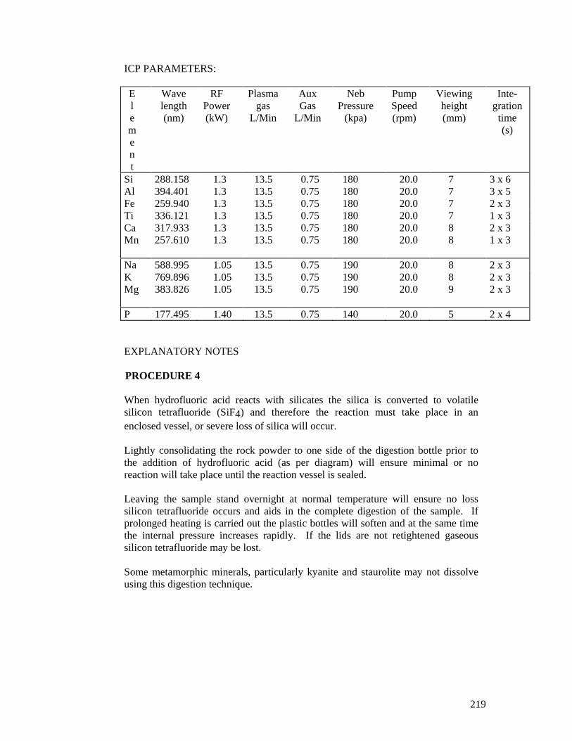
219

ICP PARAMETERS: E l e m e n t

Wave length (nm)

RF Power (kW)

Plasma gas

L/Min

Aux Gas

L/Min

Neb Pressure

(kpa)

Pump Speed (rpm)

Viewing height (mm)

Inte-gration time (s)

Si 288.158 1.3 13.5 0.75 180 20.0 7 3 x 6 Al 394.401 1.3 13.5 0.75 180 20.0 7 3 x 5 Fe 259.940 1.3 13.5 0.75 180 20.0 7 2 x 3 Ti 336.121 1.3 13.5 0.75 180 20.0 7 1 x 3 Ca 317.933 1.3 13.5 0.75 180 20.0 8 2 x 3 Mn

257.610 1.3 13.5 0.75 180 20.0 8 1 x 3

Na 588.995 1.05 13.5 0.75 190 20.0 8 2 x 3 K 769.896 1.05 13.5 0.75 190 20.0 8 2 x 3 Mg 383.826 1.05 13.5 0.75 190 20.0 9 2 x 3

P 177.495 1.40 13.5 0.75 140 20.0 5 2 x 4 EXPLANATORY NOTES

PROCEDURE 4 When hydrofluoric acid reacts with silicates the silica is converted to volatile silicon tetrafluoride (SiF4) and therefore the reaction must take place in an enclosed vessel, or severe loss of silica will occur. Lightly consolidating the rock powder to one side of the digestion bottle prior to the addition of hydrofluoric acid (as per diagram) will ensure minimal or no reaction will take place until the reaction vessel is sealed. Leaving the sample stand overnight at normal temperature will ensure no loss silicon tetrafluoride occurs and aids in the complete digestion of the sample. If prolonged heating is carried out the plastic bottles will soften and at the same time the internal pressure increases rapidly. If the lids are not retightened gaseous silicon tetrafluoride may be lost. Some metamorphic minerals, particularly kyanite and staurolite may not dissolve using this digestion technique.

220

PROCEDURE 5

The digestion bottles are cooled in a deep freeze to -15°C prior to the addition of boric acid to create a negative pressure in the bottle when the cap is removed. This reduces the possibility of any silicon tetrafluoride loss. The addition of boric acid is a critical component of the analysis. It performs the following functions; (i) It reacts with residual hydrofluoric acid to form fluoroboric acid which does not immediately react with glass. This enables the final volume of solution (200ml) to be made up in a volumetric flask. (ii) It reacts with and stabilises the volatile silicon tetrafloride and prevents any further volatilisation losses of silica. (iii) It reacts with and dissolves the precipitated calcium and magnesium fluorides formed during the digestion. (iv) Does not introduce any analyte elements into the digestion. LOSS ON IGNITION

Volatiles determined by loss on ignition will be most accurate for samples containing low concentrations of ferrous iron. The oxidation of ferrous iron during ignition increases the sample weight and if this is not subtracted from the LOI value, an incorrect result will be obtained. For samples containing low concentrations of volatiles and high concentrations of ferrous iron, the sample may actually gain weight rather than lose it after it has been ignited.

SULFUR

Sulfur is determined on the Leco R432 Sulfur analyser, by oxidation of the powdered sample in an atmosphere of pure oxygen at 1050°C, and quantitatively measuring the evolved sulfur dioxide by infra-red spectroscopy using appropriate calibrating standards.

To obtain significant results it is important the sample be ground extremely fine to ensure homogeneity of low concentration sulphides throughout the sample.

SAMPLE WEIGHT Approximately 0.250-0.300g of dried (110°C) sample is required for the Leco R432 Sulfur analyser.

221

ANALYSIS TIME Approximately 3 minutes per sample plus 3 minutes per calibrating standard and blank. REFERENCES ABBEY S. 1978. Calibration Standards. X-Ray Spectrometry, 7(2), 99-121. BERNAS B. 1968. A new method for decomposition and comprehensive analysis of silicates by atomic absorption spectrometry. Anal. Chem. 40(11), 1682. BUCKLEY D. E. & CRANSTON R. E. 1971. Atomic absorption analysis of 18 elements from a single decomposition of an aluminosilicate. Chem. Geol., 7, 273-284. EASTON A. J. 1972. Chemical analysis of silicate rocks. Elsevier Publishing Company, New York. FITTON J. G. & GILL R. C. O. 1970. The oxidation of ferrous iron in rocks during mechanical grinding. Geochim. Cosmochim. Acta 34, 518-524. FRENCH W. J. & ADAMS S. J. 1973. Polypropylene bottles in the decomposition of silicate rocks. Analytica Chimica Acta 62, 324-328. KWIECIEN W. 1990. Silicate rock analysis by AAS. School of Geology, Queensland University of Technology, Australia. LORING D. H. & RANTALA R. T. T. 1992. Manual for geochemical analysis of marine sediments and suspended particulate matter. Earth Science Reviews 32, 235-283. MAGILL W. A. & SUEHLA G. I. 1974. The study on the elimination of interferences in the determination of calcium by atomic absorption spectrophotometry. Anal. Chem. 268, 177-180. POTTS P. J. 1987. A handbook of silicate rock analysis. Chapman and Hall, New York. RANTALA R. T. T. & LORING D. H. 1989. Teflon bomb decomposition of silicate materials in a microwave oven. Anal. Chim. Acta, 220, 263-267. SAMCHUK A. I. & PILIPENKO A.T. 1987. Analytical chemistry of minerals. VNU Sciences Press, Utrecht, Netherlands.

222

APPENDIX 6 - TOTAL TRACE METAL ANALYSIS OF SEDIMENT BY HYDROFLUORIC ACID (UNIVERSITY OF QUEENSLAND)

223

Hot Plate Digestion Method applied in UQ

All acids used are concentrated and are distilled in-house and 18.2 megaohm Milli-Q water is used. All sample preparation and analytical procedures are carried out in HEPA filtered laboratories. � 100 mg of powdered sample is weighed into a PFA teflon beaker with a screw top lid and 2.5 ml of Hydrofluoric and 1 ml of Nitric acid is added. The lid is screwed on and the beaker left on a hot plate at 130C overnight. � The lid is removed and the solution dried down. � 1ml of Nitric acid is then added and dried down. � Another 1 ml of Nitric acid is added and dried down. � 2 ml of Nitric acid and 5ml of Milli-Q water is added and the lid screwed on and the beaker is left on a hotplate overnight at 100C. The solution is checked to ensure no insoluble fluorides remain. � 2 g of a 500ppb solution of internal standards is added to a cleaned 125ml LDPE bottle, the sample solution is added and then Milli-Q is added to give a total solution weight of 100g. The internal standards used are Rh, In, Re, Bi and artificially enriched isotopes of Li (6), Sr (84), Sm (147) and U (235). Samples were analysed on a Fisons PQ2+ Plasmaquad ICP-MS. Instrument operating parameters and data reduction procedures are as described in Eggins et al. (1997), except Tm is not used as one of the internal standards and a dolerite standard, W-2, was used for external calibration. Concentrations used for W-2 were derived partly by analysing it relative to synthetic standards (Li, Cr, Ni, Ga, Rb, Sr, Y, Zr, Nb, Cs, Ba, Hf, Ta, Pb, Th, U) or are based on an assessment of published, mainly ID-TIMS, data. Long-term reproducibility for the elements Li and Ga to U is about 1% and for Be to Zn is 2% to 4% as determined by repeated analyses of multiple digestions of basalt standards. REFERENCE EGGINS, S.M., WOODHEAD, J.D., KINSLEY, L.P.J., MORTIMER, G.E., SYLVESTER, P., MCCULLOCH, M.T., HERGT, J.M. & HANDLER, M.R. 1997. A simple method for the precise determination of >40 trace elements in geological samples by ICPMS using enriched isotope internal standardisation. Chemical Geology 134: 311-326,

224

APPENDIX 7 - TOTAL ELEMENT ANALYSIS BY X-RAY FLUORESCENCE SPECTROMETRY (XRF) (JAMES COOK UNIVERS ITY)

225

METHOD X-ray fluorescence (XRF) analysis provides analysis of the bulk sample in the solid form. Samples are usually prepared as fused discs (usually for major element analysis) and pressed powder pellets (for minor and trace element analysis). Both preparation methods give whole rock analysis, with none of the problems associated with the dissolution techniques cited above. XRF does have its problems with the analysis of the lighter elements and those elements tending to be volatile. For these analyses, slightly different preparation techniques are employed to keep these in the sample. Major elements (Na, Mg, Al, Si, P, S, K, Ca, Ti, Mn and Fe) are analysed with the fused disc preparation. This method minimises the mineralogical effects of the samples and produces a more accurate and precise analysis especially for the lighter elements. The glass bead from the fusion process effectively homogenises the sample so that the analysis at the surface of the bead is the same as from the bulk of the bead. This is especially important for the sodium and magnesium. However, fused beads are usually not suitable for low level analysis of trace elements: firstly because the sample is diluted, very long count times are necessary to achieve the lower limit of detection and secondly, there is usually significant contamination from the platinum crucibles that interferes with low level analysis of some elements. Therefore, trace elements are analysed from pressed powder pellets. Because most trace elements are heavy elements and thus have shorter wavelengths they are much less affected by the mineralogy of the sample and the analysis is typical of the bulk sample. JCU PREPARATION METHOD: Samples are accepted as ground powders. FUSED GLASS DISC Approximately 0.600 gms of sample is mixed with approximately 3.143 g of Norrish Hutton flux (contains La2O3) in a platinum crucible and heated at 1100oC for 15 minutes in a fusion furnace fitted with rocking device. The molten sample is quench pressed onto a graphite die and then annealed at 200oC for 30 minutes. The size of the glass disc is 28mm diameter. Weights of the sample and flux are recorded electronically for correction of the analysis for non-standard dilution. PRESSED POWDER PELLET A 5.5 gm aliquot of the ground sample is mixed with 5 drops of PVA and hydraulically pressed into an Aluminium cap. This forms a pellet of 28mm diameter. INSTRUMENTATION Both major and trace element analyses are obtained from a Bruker SRS3000 Sequential XRF Spectrometer. The Spectrometer is fitted with an Rh end-window 3kW tube, which operates under conditions suitable for each element and also a flow counter and a scintillation counter, which can be used simultaneously where possible. Analysing crystals are also chosen specific to the element. Count times and other analysing conditions are given in the results sheet. REFERENCE POTTS, P.J. 1996. A Handbook of Silicate Rock Analysis, Chapman and Hall, UK

226

APPENDIX 8 – EXTRACTABLE CATIONS IN SEDIMENTS

227

EXTRACTABLE CATIONS

IN SEDIMENT The determination of extractable cations in sediment by aqua-regia should not be confused with a total cation content. Aqua-regia (1 HNO3:3 HCl) used in this determination is unable to attack the silicate lattice therefore only adsorbed cations, oxides, hydroxides, carbonates and sulfides are digested. The following elements are routinely analysed: Cu, Pb, Co, Ni, Cr, Mo, Mn, V, Fe and Zn. Other extractable cation species may also be determined. SAFETY EQUIPMENT: Laboratory coat, safety glasses. Risk Assessments: Hydrochloric Acid (32%)/ Nitric Acid (69%)/Aqua Regia – Student usage APPARATUS:

50 mL test tubes with a 25mL calibration mark, 50 mL test tube uncalibrated, Whatman glass microfibre filters (GF/A), water bath,

REAGENTS:

SAFETY: Always use concentrated acids in an operational fume cupboard. Avoid inhalation of acid fumes. Hydrochloric Acid: Concentrated HCl (32%). Nitric Acid: Concentrated HNO3 (69%)

PROCEDURE: 1. Oven dry samples at 100-110oC until moisture free: usually overnight

depending upon volume and nature of sediment. 2. Accurately weigh 1.000 g of -80 mesh dried sediment onto a plastic weigh dish

and quantitatively transfer the sample into a 50 mL digestion tube graduated to 25 mLs. Transfer test tubes to a stainless steel test tube rack for digestion.

3. Add 1 mL conc HNO3 from an automatic acid dispenser and allow any vigorous effervescence to cease before continuing.

Add 3mLs conc HCl from automatic acid dispenser and allow any vigorous effervescence to cease before continuing.

4. SAFETY: Digestions must be carried out in an operational fume cupboard, ie set up water bath in a fume cupboard. Immerse racks into a water bath preset at about 50oC and observe reaction for at least 10 minutes. If reaction mixture effervesces vigorously, and rises rapidly above the 25 mL graduation mark, remove rack from water bath immediately and allow reaction to subside before re-entering into bath. if only one or two tubes react in this manner the reaction may be slowed down by the addition of a few mLs of distilled water from a wash bottle.

228

Increase the temperature of the water bath to 95oC and digest samples for 4 hours.

5 Allow samples to cool, add distilled water and make up to the 25 mL calibration mark. Swirl each test tube vigorously to intermix contents.

6. Re-label a series of 50 mL test-tubes in exactly the same sequence as the digested samples.

7. Filter the mixture through Whatman 41 papers or Whatman glass micro fibre filters GF/A.

8 Transfer filtered samples to plastic coated test-tube rack and seal test tubes with plastic inset caps or plastic wrap.

9. Determine trace element content in samples by ICP-OES analysis using an aqua regia blank and calibrating standards containing approximately the same matrix materials as the soil samples.

REFERENCES

LORING D. H. & RANTALA R. T. T. 1992. Manual for geochemical analysis of

marine sediments and suspended particulate matter. Earth Science Reviews 32, 235-283.

229

APPENDIX 9 - ORGANIC CARBON BY W ALKEY-BLACK METHOD

230

APPARATUS: 1 x 50 mL burette, 10mL pipette, 2 x 100mL volumetric flask, 500 mL conical

flasks SAFETY EQUIPMENT: Laboratory Coat, safety glasses, rubber gloves and fume cupboard. WARNING:

This procedure involves the use of strong acid and oxidising agents. Rubber gloves must be worn for all parts of this procedure.

Risk Assessment/s: Potassium Dichromate – Student usage Potassium Dichromate Solution – Student usage Orthophosphoric Acid – Student usage Sulfuric Acid – Student usage Sodium Fluoride – Student usage Barium Diphenylamine-4-sulphonate – Student usage REAGENTS: Orthophosphoric Acid: 85% H3PO4 Sodium Fluoride: Solid NaF Silver Sulfate and Sulfuric Acid: Weigh 1.25g Ag2SO4 into a 500 mL glass

bottle. Add 200 mL of conc. H2SO4. Shake to dissolve Ag2SO4. Add another 800 mLs of conc. to give a total of 1000 mLs H2SO4.

Standard 1 N Potassium Dichromate Solution: Weigh exactly 49.04g of

K2Cr2O7 and dilute to 1000 mL in a volumetric flask. 0.5 N Ferrous Solution: Weigh exactly 196.1 g of Fe(NH4)2SO4.6H2O.

Dissolve in 20 mL H2SO4. Transfer to a 1000 mL volumetric flask and dilute to the mark.

Diphenylamine Indicator: Weigh 0.5 g of Diphenylamine or BDS and

dissolving 20 mL of water and 100 mL of conc. H2SO4. PROCEDURE: 1) Weigh 0.5 g of dried dextrose into a 500 mL conical flask. 2) Add exactly 10 mL of 1 N K2Cr2O7 by pipette. 3) Add 20 mL of the H2SO4/Ag2SO4 mix. SAFETY: This must be

carried out in an operating fume cupboard. Mix by gently rotation flask to ensure complete mixing of reagents and sample while avoiding splashing sample onto sides of the flask out of contact with reagents.

4) Let mixture stand for 10 mins. 5) Add 200 mLs of distilled water, 10 mLs of 85% H3PO4 and 0.2g of

231

NaF. 6) Add 15 drops of BDS indicator. 7) Titrate the solution with 0.5 N Ferrous solutions to a brilliant green

end point. During the titration the solution will change from an opaque green-brown to bluish-black-grey and finally to a one drop end point of brilliant green.

8) Prepare a blank by adding all reagents except the sediment sample to the conical flask and treat using the same procedure as above.

DISPOSAL: All solutions containing chromium must be disposed of into the heavy metal

residues collection bottle located in the fume cupboards. CALCULATION:

% C = 10 (1 - T/B) x F

Where: B = standardisation blank titration (mL of ferrous

solution) T = Sample titration (mL of ferrous solution) F = (1.0 N) x 12/4000 x 1.72 x 100 / sample weight Standardisation of this procedure may be performed by following the procedure

using 0.01g dextrose instead if sediment sample. (Dextrose should contain 39.99% C.) The calculation is as above except:

F = (1.0 N) x 12/4000 x 100 / sample weight REFERENCE: LORING, D.H. and RANTALA, R.T.T. 1992 Manual for geochemical analyses of marine sediments and suspended particulate matter, Earth Science Reviews 32: 235 - 283.

232

APPENDIX 10 - X-RAY DIFFRACTION ANALYSIS

233

X-RAY DIFFRACTION ANALYSIS GENERAL XRD is a widely used technique for mineral identification, particularly for fine-grained materials where the grain size is too small to be usefully studied with the optical microscope. In addition, the XRD analysis can provide information on the degree of structural disorder, particle size, and the nature of isomorphous substitutions. The method is based on the fact that X-rays are scattered by the electrons around atoms, which form the atomic layers in crystals (lattice spacings). A particular crystalline material has a particular structure or lattice. The scattered x-rays reinforce each other in directions that depend on the lattice repeat distances and the wavelength of the x-rays. The angles of diffraction give an indirect indication of the spacings (d spacings) between atomic layers and therefore can be used for mineral identification. The advantages of the method include the fact that: 1) It is non-destructive, 2) The samples are reasonably easy to prepare, 3) The material can be processed even in very small quantities, 4) Modern computer-linked instruments are quite straightforward to operate and

maintain. The limitations of the XRD analysis include: 1) The method is capable of identifying only crystalline materials, 2) Components of the same mineral series (i.e. micas, feldspars, amphiboles) which

have very similar crystallographic structures are difficult to separate due to their very similar XRD patterns.

MICRONIZING The micronizing vessel consists of a plastic cylinder filled with 48 stacked small agate or corundum cylinders. The particle size of the sample material to be crushed in this type of mill is to be no larger than 100 microns (i.e. what is obtainable from a swing mill). Approximately 3 g of sample and 10-12 ml of alcohol are placed into the micronization vessel and then into the arm of the mill. The timer on the mill is typically set to 0.2 (hr) (i.e. 12 minutes). Other settings of the timer can be made. The slurry obtained is homogenous and the particle size is ideally in the range of 1 to 5 microns. The mixture of sample/alcohol is placed in a pre-labelled beaker and left to dry overnight in an oven at 50-600 C. The sample will require remixing prior its use to counteract any segregation of phases during the drying step. The micronized powder is used to identify all the mineral phases of the sample providing that the phases are present in sufficient abundance. RANDOMLY ORIENTATED POWDER SAMPLES About 1.5-2 g of powder is lightly packed (to avoid as much as practical pressure orientation), into the backside of a circular cavity of an aluminium plate. The front

234

face of the sample holder rests on a polished metal block. The pressing is done using a small plastic cylinder and a metal ring for guidance. After the powder is packed, the plastic cylinder and metal ring are removed and the second half of the holder is carefully clicked on. The entire holder is then lifted, inverted and placed face upward into the auto sample changer carousel. When the entire batch is ready, the carousel is placed into the auto sample changer and the data acquisition task begun. ORIENTATED SPECIMENS Preparation of orientated samples is suitable and sometimes absolutely necessary for identification of clay minerals. Clay silicates have a particular structure developed along the (001) crystallographic plane, which makes them difficult to identify in a non-orientated (random) sample preparation, especially when the clay phases are in small quantities. The mechanism of orientating clay crystals exploits their sheet structure and to make the sheets lay one atop of the other in the same plane. This produces a pseudo-macrocrystal and creates a more intense diffraction pattern of the (001) basal spacing series. The first step is to disperse the sample in about ten times its volume of distilled water. Light grinding and shaking of the mixture (or ultrasonic dispersion) leads to a dissociation of the clay particles and separation of clay size material from the coarser (mineral) fractions. The material left in suspension is generally finer than 2 microns and can be taken with a pipette, spread over a glass slide and the slide then placed on top of a warm surface to dry. In about an hour at 500 C, the water evaporates leaving behind a gravimetrically deposited clay fraction. The glass slide is placed on a plastic holder, which fits on the back of the Co-machine holders. REFERENCES JENKINS R. & SNYDER R. L. 1996. Introduction to X-ray Powder Diffractometry, Chapter 9 (Specimen preparation), Chemical Analysis, Vol. 138, pp. 231-259, Wiley. BISH D. L. & POST J. E. 1989. Sample Preparation for X-ray Diffraction, Chapter 4 (Modern powder X-ray diffraction), Rev. Mineral, Vol 20, pp. 72-99. Mineral Soc. Am., Washington DC. NOTE The identification and quantification of sediment mineral phases presented in this thesis was assisted by several computer programs: 1) TRACES (plot of XRD traces, locate peaks and export data), 2) JADE (search-match program) and 3) SIROQUANT (quantification program which expresses the composition of the sample in percentages of dry weight). The error of the quantification was calculated as Chi Squared (goodness of fit between the experimental XRD trace and the calculated one) and ranged between 3 and 7.

235

APPENDIX 11 - CATIONS IN WATER, INDUCTIVELY COUPLED PLASMA- OPTICAL EMISSION SPECTROSCOPY (ICP-OES)

236

Cations in Water by Inductively Coupled Plasma – Optical Emission

Spectroscopy (ICP – OES) Cations were analysed by a Varian Liberty 200 inductively coupled plasma optical emission spectrometer (ICP – OES). The instrument was calibrated using synthetic standards. Major cations analysed were Na, K, Ca and Mg; minor and trace cations were Fe, Al, Zn, Cu, Mn, Sr, Ba, Ti, Li and V. Silica, although not in ionic form in natural waters, was also analysed with this suite of cations. The detection limits used are shown in Table 1. Major Cations: Na, K, Mg and Ca Minor Cations: Al, Si, Sr, Mn, Fe, Zn and Cu Table 1. Detection limits. Element

Working Detection Limits

Na 0.015 – 1500 mg/L

K 0.20 – 150 mg/L

Mg 0.001 – 150 mg/L

Ca 0.0003 – 250 mg/L

Al 0.015 – 75 mg/L

Si 0.011 – 75 mg/L

Sr 0.0006 – 75 mg/L

Mn 0.003 – 7.5 mg/L

Fe 0.015 – 7.5 mg/L

Zn 0.009 – 7.5 mg/L

Cu 0.02 – 0.75 mg/L

THEORY OF OPERATION: The cation and sulfur concentrations are measured using inductively coupled plasma - optical emission spectroscopy (ICP-OES). This technique involves the water sample being aspirated into a plasma. The intensity of characteristic wavelengths emitted by the excited analyte ions in the plasma are measured by a spectrophotometer. The measured intensity is proportional to concentration, thus concentration of ions in the sample can be determined. SAMPLE PREPARATION: Little or no sample preparation is required for analysis of aqueous samples by ICP-OES except for highly turbid samples, which must be filtered and samples of high

237

conductivity, which must be diluted to <4000 µS before analysis. Also, concentration of elements determined must be within the detection limits of the ICP-OES for the results to have analytical meaning. Filter turbid samples through a 0.45 or 0.8 µm membrane filter, collect and analyse the filtrate, diluting if necessary. It is possible for cations other than those listed above to be analysed, however it may not be feasible if the selected analyte ions are present only in trace amounts i.e. at levels below the limits of ICP-OES detection. ANALYTICAL ERROR: Approximate error (based on repeat analyses) of approximately 5%.

238

APPENDIX 12 - ANIONS IN WATER BY ION CHROMATOGRAPHY (IC)

239

Anions in Water by Ion Chromatography (IC)

The following anions, chloride, sulfate, nitrate, phosphate and bromide, have been determined by ion chromatography (IC) using a Dionex DX 300 ion chromatograph with suppressed conductivity detection. The system utilises Dionex AS14 analytical column and AG14 guard column. Conductivity suppression was by a micromembrance suppressor, Dionex CMMS-II. Cl-, SO4

2-, Fl-, Br-, NO3- and PO4

3- (NO2

- and SO32- can also be analysed but are not included in the routine analysis.)

DECTECTION LIMITS: A working range has been given below. This range is based on a combination of standard concentration range and instrument working range. Fl- 0.05 to 12 ppm Cl- 0.5 to 150 ppm SO4

2- 0.5 to 100 ppm Br- 0.05 to 12 ppm NO3

- 0.05 to 12 ppm PO4

3- 0.05 to 12 ppm THEORY OF OPERATION: THE ION CHROMATOGRAPHIC PROCESS: The sample is introduced in the flowing stream and carried into the anion exchange column. Ions interact with the ion exchange sites on the stationary phase in the column. Mobile phase ions (or eluent ions) compete with the sample ions for ion exchange sites on the column. Separation depends upon the different ions having different affinities for both phases. In the case of anion separations the differing affinities for stationary and mobile phases are due to the ionic charge and ion size (ionic radius) of each anion species. Once anions are separated the concentration of each species present in the sample is measured using a conductivity detector. A chromatogram displays peaks in conductivity at various retention times. Each anionic species is identified by its retention time, which remains constant throughout successive runs. STATIONARY PHASE: the column packing material containing functionalised active sites. For anion determinations the Dionex AS14 anion exchange column is used. MOBILE PHASE (OR ELUENT): The liquid flowing though the column that contains competing ion for the active sites. SAMPLE PREPARATION: Little of no sample preparation is required of analysis of aqueous sample by ion chromatography. However highly turbid samples must be filtered before analysis

240

and sample of high conductivity require diluting before analysis. Samples analysed must have a conductivity of less than 700 µS, if not dilution is required. Filter turbid samples through a 0.45 of 0.8 um membrane filter, collect and analyse the filtrate, diluting if necessary. REAGENTS: Eluent: 3.5mM Na2CO3/1.0 mM NaHCO3. Prepare diluting the 100x concentrate 100 fold. I.e. pipette 10 mL of 100x concentrate into a 1000 mL volumetric flask and dilute to the mark with ultra pure water. (Obtain ultra pure water from the purification unit located on the back island bench located in the Geochem lab R431.) Fill eluent bottle with this solution and sparge with argon for at least ten minutes before starting eluent pump. Regenerant solution: Add 2.4 mL of conc. H2SO4 to 1000 mL of ultra pure water and dilute further to 2000mLs. Fill regent bottle with this solution recap and allow pressurising. After several minutes ensure regent solution is flowing through suppressor. RESULTS: Ion chromatography is an excellent method of anion species determination in water samples. It has an extremely good precision with a %RSD of <2%. However it is important that results obtained are not taken on face value but are checked to assure data is reasonable. This is particularly important as peaks can be misnamed due to small shifts in retention time. The retention time can change due to a variety of reasons most commonly due to problems with the eluent pump, blockages and inaccurate preparation of eluent. Always check with previous days data to determine if retention times have not changed (refer to daily log, located next to instrument for this information). Also data should be with the working range of each species listed above, if not a dilution may be requiring before rerunning samples or an alternative method of analysis may be required. In particular, high chloride data should be checked by titration as concentrations over 150-200 ppm may not be linear, giving inaccurate results.

241

APPENDIX 13 – TITRATION METHOD FOR ALKALINITY

242

Alkalinity and Acid Titration Methods

DETECTION LIMIT: 0.25 ppm CaCO3 (mg/L water) APPARATUS: 250 mL conical flask, calibrated pH meter and 25 mL burette SAFETY EQUIPMENT: Laboratory coat, safety glasses. Refer to Risk Assessment/s: Hydrochloric acid (32%) - Student usage REAGENTS: 0.1N Standard HCl: SAFETY: This dilution must be carried out in a fume

cupboard. Pipette 10 mLs of conc HCl (10 M) into a 1000 mL volumetric flask and dilute to mark.

Standardisation of 0.1 N HCl: Weigh 0.7 - 0.8 g of pure sodium tetraborate by difference into a 150 mL

conical flask, dissolve in about 50 mLs of distilled water and add a few drops of methyl red indicator. Titrate the sodium tetraborate solution with the 0.1N HCl as the titrant until the colour changes to pink. Record the volume of HCl used. Carry out this procedure in triplicate. Use the following equation to calculated the normality of the acid solution.

N HCl = Weight of Na2B4O7 / 190.72 x Vol of Titrant (HCl)

0.02 N Standard HCl: Pipette 200 mLs of standard 0.1N HCl into a 1000 mL volumetric flask and dilute to the mark.

PROCEDURE: The alkalinity of a sample is due to the presence of hydroxide, carbonate or

bicarbonate ions. The concentration of each of these ions in a sample can be calculated once the phenolphthalein and total alkalinity have been determined.

1) Determination of phenolphthalein alkalinity or P

a) Pipette 100 mLs of sample into a 250 mL beaker. Measure the pH of the sample. If pH is less than 8.3 go on to step 2) as P=0.

b) If pH is greater than 8.3 then titrate the sample with 0.1N HCl to pH

8.3. Use a magnetic stirrer and leave pH probe in sample while titrating.

243

Record volume of HCl used. Calculate alkalinity due to hydroxide, P, by

using Calculation (a). Go on to step 2).

2) Determination of total alkalinity or T

a) Titrate the sample to the pH 4.7 if the sample alkalinity is unknown. If known choose the appropriate total alkalinity equivalence point from the following table.

These pH values are suggested equivalence points for the corresponding

alkalinity concentrations.

Alkalinity (mg/L CaCO3)

End Point pH: Total

30 4.9 150 4.6 500 4.3

Silicates, phosphates known or suspected

4.5

Industrial waste or complex system

4.5

b) Record total volume of HCl titrated ie. include volume of titrant used in

step 1 if appropriate. Calculate the Total Alkalinity, T, using calculation (b). If Total Alkalinity, T, is less than 20 mg/L CaCO3 go to step 3). If Total Alkalinity, T is greater than 20 mg/L CaCO3 go to step 4.

3) Determination of Total Alkalinity less the 20mg/L CaCO3 a) Pipette 100 mLs of sample into a 250 mL beaker and titrate using

0.01M HCl to an end point in the range of 4.3 to 4.7. Record the volume and the exact pH.

b) Titrate the solution further to reduce the pH exactly 0.30 pH units and record volume. Use Calculation (c) to determine Total Alkalinity, T.

4) Determine the relationship between Hydroxide, Carbonate and Bicarbonate

Alkalinity using Table 2. NOTE: As the end point is approached make smaller additions of acid and be sure

that pH equilibrium is reached before adding more titrant. CALCULATIONS: a) P (Phenolphthalein Alkalinity) P mg/L CaCO3 = A x N x 50 000 / volume of sample where A = mL standard acid used N = normality of standard acid b) T (Total Alkalinity)

244

T mg/L CaCO3 = A x N x 50 000 / volume of sample where A = mL standard acid used N = normality of standard acid c) Potentiometric titration of low alkalinity (<20mg/L CaCO3): T (Total alkalinity), T mg/L CaCO3 = (2B - C) x N 50 000 / volume of sample where B = mL of titrant to first recorded pH C = total mL of titrant of reach pH 0.3 unit lower N = normality of acid Table 2 Calculation of alkalinity relationships

Result of titration Hydroxide Alkalinity as CaCO3

Carbonate Alkalinity as CaCO3

Bicarbonate Alkalinity as CaCO3

P = 0 0 0 T P < 1/2T 0 2P T - 2P P >=1/2T 0 2P 0 P > 1/2T 2P-T 2(T-P) 0

P=T T 0 0 Where P = phenolphthalein alkalinity T = total alkalinity Report total alkalinity as: "The alkalinity to pH ____ = ____ mg CaCO3/L" To convert hydroxide, carbonate and bicarbonate expressed as alkalinity to concentration of their own species to be used in a mass balance multiply by the following factors.

Hydroxide mg/L OH- = mg/l CaCO3 x 0.34

Carbonate mg/L CO32- = mg/L CaCO3 x 0.60

Bicarbonate mg/L HCO3- = mg/L CaCO3 x 1.22 REFERENCE

GREENBERG A. E., CLESCERI L. S. & EASTON A. D. 1992. Standard methods

for the examination of water and wastewater. 18th Ed. APHA. AWWA. WEF.

245

APPENDIX 14 – ADDITIONAL LABORATORY ANALYSIS DATA

246

These additional data complement Paper 2. The samples were analysed following

the procedures described in the paper and Appendices 5 (HF) & 7 (XRF).

0 1.5 3

kilometres

Weathered bedrock

Alluvium

weathered profilesSand

Clay rich in organic matter

Brib

ie Is

land

Lamerough Ck

Bells North Arm Ck

Bel ls South Arm Ck

Halls Ck

N

Coral Sea

S1

B3

GB1

Caloundra

Pum

ices

tone

Pas

sage

Queensland

0 1.5 3

kilometres

Weathered bedrock

Alluvium

weathered profilesSand

Clay rich in organic matter

Brib

ie Is

land

Lamerough Ck

Bells North Arm Ck

Bel ls South Arm Ck

Halls Ck

NN

Coral Sea

S1

B3

GB1

Caloundra

Pum

ices

tone

Pas

sage

Queensland

Figure 1. Location of sample sites studied in paper 2.

247

Table 1: A comparison between XRF and HF methods for major element

concentrations (%)

Sample Na2O K2O MgO CaO TiO2 MnO Fe2O3 Al2O3 SiO2

XRF HF XRF HF XRF HF XRF HF XRF HF XRF HF XRF HF XRF HF XRF HF

S1-2 bd 0.2 1.2 1.5 0.4 0.5 0.1 0.02 0.8 0.7 bd 0.01 6.2 7.1 16.4 19 67.1 66

S1-5 0.8 0.8 2.0 2.4 0.7 0.9 0.2 0.3 0.5 0.6 bd 0.1 3.0 3.6 11.2 13 75.9 76

B3-1 2.2 2.4 1.9 2.1 0.4 0.4 0.3 0.3 0.5 0.4 0.1 0.1 2.3 2.4 10.2 11 78.9 80

B3-4 2.1 2.2 1.5 1.5 0.6 0.6 1.1 1.2 0.5 0.4 0.2 0.2 4.1 4.1 9.0 9.1 75.9 76

GB1-3 0.5 0.5 0.2 0.1 0.8 0.2 0.2 0.2 2.9 3.4 bd 0.02 22.7 24 18.1 18 38.9 39

GB3-5 1.9 2.1 1.4 1.6 0.5 0.2 0.2 0.2 0.8 0.9 bd 0.02 2.7 3.2 10.3 12 78.9 79

Table 2: A comparison between XRF (%) and HF (mg/kg) methods for trace metal

concentrations

Sample VXRF VHF CrXRF CrHF CoXRF CoHF NiXRF NiHF CuXRF CuHF ZnXRF ZnHF PbXRF PbHF

S1-2 78 75 76 42 1 1 5 10 bd 1 24 11 5 12

S1-5 67 53 85 29 18 16 15 23 14 15 105 117 10 17

B3-1 67 43 75 37 12 10 8 15 6 5 97 103 4 13

B3-4 59 43 78 20 12 12 10 18 6 4 49 49 4 11

GB1-3 259 290 1056 842 47 35 227 196 51 60 97 93 5 7

GB3-5 95 63 157 75 30 23 67 66 15 16 90 86 3 12

248

The following data are the analyses of soil and sediment samples (locations in the attached figure) following the procedures in Appendices 5 (Sulfur), 8 (extractable method) & 9 (OC) and complement Paper 3.

Soil developed on sandstone bedrock from QASSIT Sample V Cr Mo Ni Cu Zn Pb Fe Mn Al S OC 570-0* 5.4 5.7 1.8 1.4 0.7 30 5 3336 3 5767 0.05 2.2 570-140 3.2 16.2 2.6 4.1 1.3 35 1 995 3 1903 0.04 0.5 570-220 2.6 6.3 1.8 4.7 bd 38 1 1492 2 2677 0.10 0.2 566-0 1.8 6.1 1.1 0.5 0.6 24 2 831 1 537 0.02 0.8 566-50 13.4 6.6 0.8 bd bd 44 4 7523 2 6263 0.02 0.3 566-180 7.5 4.6 3.9 0.0 0.6 48 5 2040 1 4939 0.03 0.1 566-380 9.2 5.6 0.8 0.8 bd 52 3 8596 1 5855 0.02 0.0 565-0 14.0 15.8 6.2 3.2 12.5 35 19 4553 6 19342 0.07 7.2 565-80 7.1 4.8 5.6 0.2 0.8 40 7 2099 2 4726 0.04 0.6 565-380 2.5 3.0 1.9 1.5 bd 43 5 2459 18 3634 0.02 0.1 561-0 3.6 5.6 2.2 0.9 0.6 41 2 2604 3 2135 0.00 1.3 561-80 23.9 13.0 4.6 1.7 bd 43 2 9350 3 10071 0.02 0.1 561-180 4.4 4.3 4.8 0.0 0.5 35 7 1128 1 5585 0.04 0.0 561-280 18.1 5.5 2.5 bd bd 39 4 7198 5 7780 0.03 0.5 560-0 2.0 1.7 0.6 0.5 bd 21 0 1255 2 960 0.01 1.7 560-80 2.6 3.8 bd 1.1 bd 22 0 1300 1 1239 0.01 2.7 560-180 9.1 10.4 0.4 3.4 1.1 30 5 2200 4 4697 0.02 0.8 660-0 11.7 5.7 0.3 1.3 bd 36 8 8288 6 8828 0.05 3.9

660-130 5.0 5.9 1.7 1.1 1.0 32 0 1094 3 3223 0.04 0.6 663-0 8.7 4.6 0.0 1.1 0.8 54 6 3755 7 6819 0.08 8.6 663-50 4.0 2.8 1.0 0.5 bd 39 2 1092 2 3737 0.03 2.4 663-180 5.6 4.7 0.5 0.0 bd 28 2 1530 3 4854 0.03 0.6 1120-0 40.8 14.6 14.4 2.4 14.5 30 6 27001 21 11343 0.05 4.1 1120-50 19.7 9.8 1.7 1.6 bd 25 3 4121 5 8468 0.02 0.7 1120-180 25.1 8.7 1.5 0.7 bd 23 3 755 2 4576 0.03 0.8

* Indicates depth of sampling bd=below detection limit all in mg/kg except for S in %

249

Soils with estuarine origin from QASSIT Sample V Cr Mo Ni Cu Zn Pb Fe Mn Al S OC 573-0* 10.5 10.4 6.4 4.2 2.4 54 17 3848 16 22592 0.13 7.8 573-80 10.2 12.6 4.0 5.9 1.7 61 16 3785 10 28112 0.13 5.3 573-140 6.8 7.0 1.8 2.5 0.7 44 bd 2964 9 3567 0.54 3.6 573-170 7.9 8.8 1.5 4.3 1.1 62 4 8585 32 5692 1.01 4.2 573-210 3.6 6.5 2.4 2.9 0.5 32 bd 3485 12 2099 0.48 1.0 573-250 4.6 10.7 2.3 4.1 0.7 28 3 3866 14 3296 0.44 2.1 542-0 4.5 25.0 3.3 8.3 0.6 47 bd 3522 5 2825 0.03 2.5 542-80 7.0 30.3 1.5 8.3 0.5 36 bd 1114 5 5055 0.02 0.4 542-230 2.1 43.8 2.9 13.4 0.5 40 4 774 4 5757 0.03 0.0 563-0 21.7 13.8 2.7 3.0 1.3 46 11 5214 14 21946 0.14 10.1 563-50 13.1 14.2 5.0 2.1 0.7 25 9 1523 4 17687 0.09 5.1 563-130 2.5 5.5 2.6 0.0 0.5 40 10 670 3 8836 0.03 5.7 545-0 2.3 95.0 2.1 36.0 1.0 27 bd 2431 8 1016 0.02 2.6 545-80 0.6 5.0 1.0 bd 0.8 41 bd 624 1 260 0.01 0.1 545-160 1.2 5.0 1.0 bd 1.4 38 bd 660 1 1143 0.06 2.7 562-0 33.3 23.6 4.9 4.3 2.9 45 9 7165 12 12716 0.10 2.0 562-80 42.6 22.5 2.9 3.3 3.0 29 4 11534 15 10179 0.12 1.5 562-130 29.1 20.1 7.8 2.3 3.0 35 10 4065 11 8629 0.14 1.0 562-230 47.7 21.2 1.0 2.5 0.7 35 11 21329 117 12264 0.07 0.8 651-0 4.9 2.4 1.0 bd 0.8 31 bd 491 2 1058 0.07 1.3

651-130 17.0 11.3 1.1 bd 1.1 28 bd 15742 5 3473 0.03 0.4 651-330 34.6 32.6 2.3 3.4 3.4 41 10 2312 14 12293 0.15 1.7 509-0 0.7 35.4 1.0 10.7 0.8 23 bd 471 4 286 0.06 4.1

509-130 2.5 38.7 1.0 14.6 1.8 34 bd 578 5 3564 0.08 1.3 509-280 1.6 14.1 1.0 5.0 0.6 22 bd 543 2 799 0.05 0.3 652-0 0.7 1.4 1.0 bd 0.5 23 bd 278 2 228 0.02 3.0

652-230 1.4 1.8 1.0 bd 0.5 29 bd 231 0 1176 0.06 1.8 652-480 31.4 28.0 1.5 9.4 3.7 45 11 18435 35 15043 1.54 4.4 569-0 19.6 17.1 2.7 4.9 3.6 33 4 8086 7 7638 0.11 7.1

569-130 5.9 6.6 1.0 1.8 1.5 38 bd 2140 6 2583 0.07 0.7 569-280 14.0 11.6 1.0 5.0 2.6 45 bd 9973 36 5954 0.38 1.2 569-370 16.2 10.2 1.8 5.0 2.0 31 3 10924 26 5714 0.60 2.2 661-0 29.0 19.2 3.7 5.0 0.5 58 5 9426 11 15404 0.11 9.2 661-80 45.0 46.6 4.8 7.3 5.8 63 12 35105 22 23478 0.06 2.2 661-230 6.9 5.3 1.0 4.6 1.0 27 bd 5799 23 3765 0.44 1.4 659-100 8.0 5.6 1.0 1.3 0.8 42 7 2182 5 9066 0.09 7.8 659-230 11.5 8.2 1.0 2.5 1.3 34 9 2633 6 10138 0.09 6.8 659-330 12.3 6.8 1.0 2.8 2.0 34 8 2916 7 7507 0.44 10.2 662-0 34.6 14.0 15.3 6.8 0.9 35 12 34064 13 16322 0.20 10.3 662-70 15.4 8.6 1.0 8.6 1.5 36 5 14619 15 4750 1.52 3.6 662-180 4.7 4.2 1.0 bd 0.5 44 bd 392 2 3198 0.04 0.9 655-0 0.4 1.0 1.0 bd 0.5 22 bd 179 1 210 0.02 1.9 655-80 1.1 4.6 1.1 1.5 0.5 20 bd 261 1 1589 0.02 2.2 655-330 2.7 2.8 1.8 3.8 1.0 29 bd 2503 5 1633 0.21 0.6 655-380 23.3 11.8 3.2 3.7 0.6 31 16 4080 8 18405 0.12 0.8

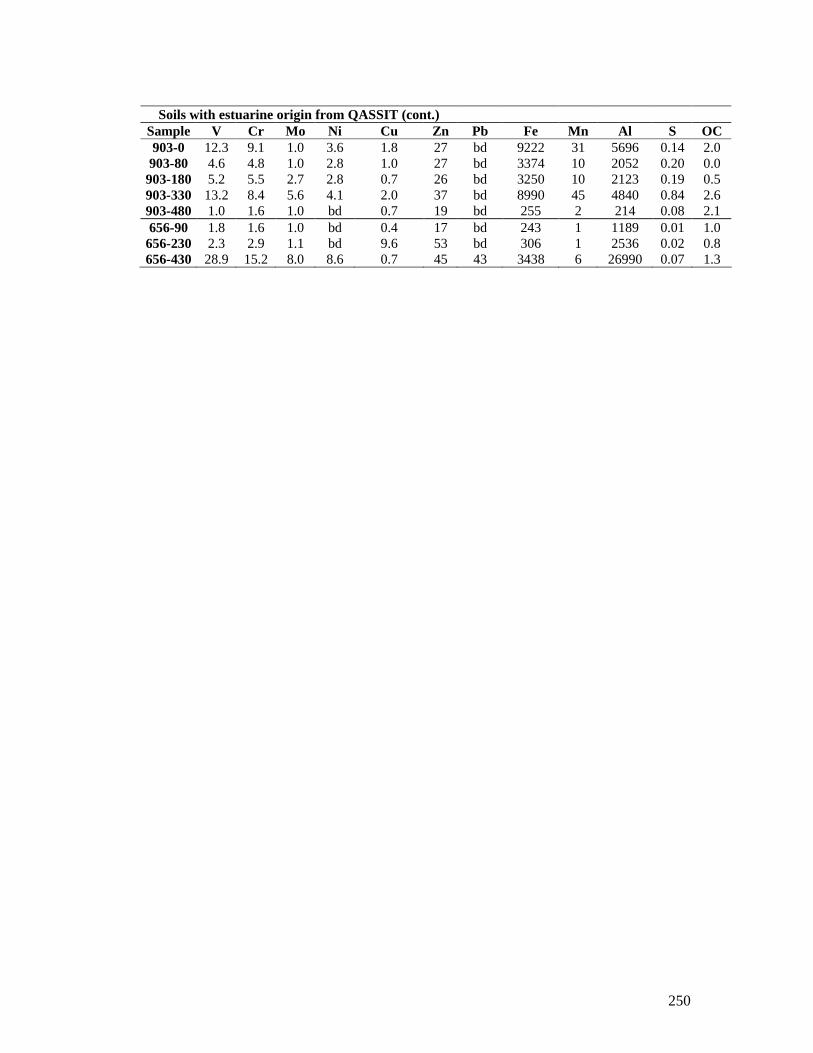
250

Soils with estuarine origin from QASSIT (cont.)

Sample V Cr Mo Ni Cu Zn Pb Fe Mn Al S OC 903-0 12.3 9.1 1.0 3.6 1.8 27 bd 9222 31 5696 0.14 2.0 903-80 4.6 4.8 1.0 2.8 1.0 27 bd 3374 10 2052 0.20 0.0 903-180 5.2 5.5 2.7 2.8 0.7 26 bd 3250 10 2123 0.19 0.5 903-330 13.2 8.4 5.6 4.1 2.0 37 bd 8990 45 4840 0.84 2.6 903-480 1.0 1.6 1.0 bd 0.7 19 bd 255 2 214 0.08 2.1 656-90 1.8 1.6 1.0 bd 0.4 17 bd 243 1 1189 0.01 1.0 656-230 2.3 2.9 1.1 bd 9.6 53 bd 306 1 2536 0.02 0.8 656-430 28.9 15.2 8.0 8.6 0.7 45 43 3438 6 26990 0.07 1.3

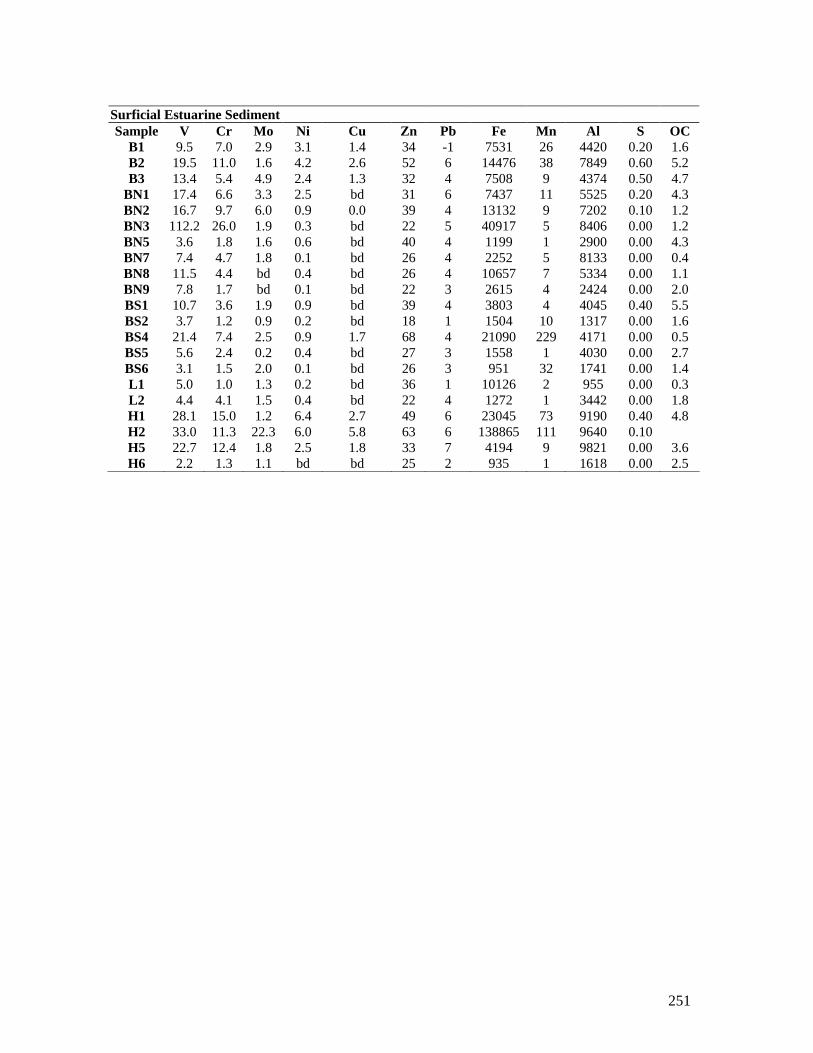
251

Surficial Estuarine Sediment Sample V Cr Mo Ni Cu Zn Pb Fe Mn Al S OC

B1 9.5 7.0 2.9 3.1 1.4 34 -1 7531 26 4420 0.20 1.6 B2 19.5 11.0 1.6 4.2 2.6 52 6 14476 38 7849 0.60 5.2 B3 13.4 5.4 4.9 2.4 1.3 32 4 7508 9 4374 0.50 4.7

BN1 17.4 6.6 3.3 2.5 bd 31 6 7437 11 5525 0.20 4.3 BN2 16.7 9.7 6.0 0.9 0.0 39 4 13132 9 7202 0.10 1.2 BN3 112.2 26.0 1.9 0.3 bd 22 5 40917 5 8406 0.00 1.2 BN5 3.6 1.8 1.6 0.6 bd 40 4 1199 1 2900 0.00 4.3 BN7 7.4 4.7 1.8 0.1 bd 26 4 2252 5 8133 0.00 0.4 BN8 11.5 4.4 bd 0.4 bd 26 4 10657 7 5334 0.00 1.1 BN9 7.8 1.7 bd 0.1 bd 22 3 2615 4 2424 0.00 2.0 BS1 10.7 3.6 1.9 0.9 bd 39 4 3803 4 4045 0.40 5.5 BS2 3.7 1.2 0.9 0.2 bd 18 1 1504 10 1317 0.00 1.6 BS4 21.4 7.4 2.5 0.9 1.7 68 4 21090 229 4171 0.00 0.5 BS5 5.6 2.4 0.2 0.4 bd 27 3 1558 1 4030 0.00 2.7 BS6 3.1 1.5 2.0 0.1 bd 26 3 951 32 1741 0.00 1.4 L1 5.0 1.0 1.3 0.2 bd 36 1 10126 2 955 0.00 0.3 L2 4.4 4.1 1.5 0.4 bd 22 4 1272 1 3442 0.00 1.8 H1 28.1 15.0 1.2 6.4 2.7 49 6 23045 73 9190 0.40 4.8 H2 33.0 11.3 22.3 6.0 5.8 63 6 138865 111 9640 0.10 H5 22.7 12.4 1.8 2.5 1.8 33 7 4194 9 9821 0.00 3.6 H6 2.2 1.3 1.1 bd bd 25 2 935 1 1618 0.00 2.5

252

Mineralogical data for selected samples complementing Paper 3. Samples (locations

in the attached figure) were analysed following a procedure in Appendix 10.

Soil developed on sandstone bedrock Sample Quartz Feldspars Kaolinite Mixed

layer Illite Pyrite Hematite NaCl Goethite Jarosite Anatase

1120-0 77.4 2.8 17.1 2.0 0.0 0.0 0.7 0.0 0.0 0.0 traces 1120-50 81.1 1.1 17.8 0.0 0.0 0.0 0.0 0.0 0.0 0.0 traces 1120-180 78.3 1.1 20.6 0.0 0.0 0.0 0.0 0.0 0.0 0.0 traces

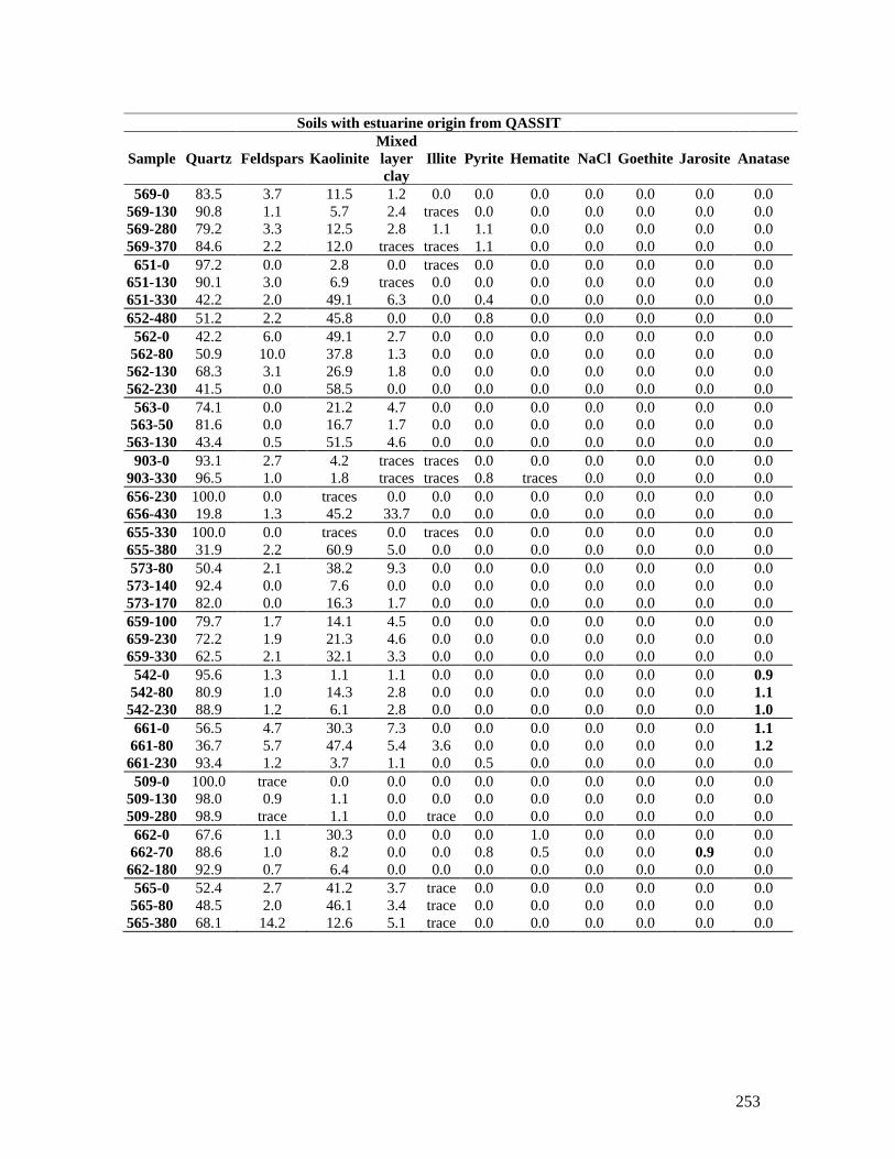
253

Soils with estuarine origin from QASSIT

Sample Quartz Feldspars Kaolinite Mixed layer clay

Illite Pyrite Hematite NaCl Goethite Jarosite Anatase

569-0 83.5 3.7 11.5 1.2 0.0 0.0 0.0 0.0 0.0 0.0 0.0 569-130 90.8 1.1 5.7 2.4 traces 0.0 0.0 0.0 0.0 0.0 0.0 569-280 79.2 3.3 12.5 2.8 1.1 1.1 0.0 0.0 0.0 0.0 0.0 569-370 84.6 2.2 12.0 traces traces 1.1 0.0 0.0 0.0 0.0 0.0 651-0 97.2 0.0 2.8 0.0 traces 0.0 0.0 0.0 0.0 0.0 0.0

651-130 90.1 3.0 6.9 traces 0.0 0.0 0.0 0.0 0.0 0.0 0.0 651-330 42.2 2.0 49.1 6.3 0.0 0.4 0.0 0.0 0.0 0.0 0.0 652-480 51.2 2.2 45.8 0.0 0.0 0.8 0.0 0.0 0.0 0.0 0.0 562-0 42.2 6.0 49.1 2.7 0.0 0.0 0.0 0.0 0.0 0.0 0.0 562-80 50.9 10.0 37.8 1.3 0.0 0.0 0.0 0.0 0.0 0.0 0.0 562-130 68.3 3.1 26.9 1.8 0.0 0.0 0.0 0.0 0.0 0.0 0.0 562-230 41.5 0.0 58.5 0.0 0.0 0.0 0.0 0.0 0.0 0.0 0.0 563-0 74.1 0.0 21.2 4.7 0.0 0.0 0.0 0.0 0.0 0.0 0.0 563-50 81.6 0.0 16.7 1.7 0.0 0.0 0.0 0.0 0.0 0.0 0.0 563-130 43.4 0.5 51.5 4.6 0.0 0.0 0.0 0.0 0.0 0.0 0.0 903-0 93.1 2.7 4.2 traces traces 0.0 0.0 0.0 0.0 0.0 0.0

903-330 96.5 1.0 1.8 traces traces 0.8 traces 0.0 0.0 0.0 0.0 656-230 100.0 0.0 traces 0.0 0.0 0.0 0.0 0.0 0.0 0.0 0.0 656-430 19.8 1.3 45.2 33.7 0.0 0.0 0.0 0.0 0.0 0.0 0.0 655-330 100.0 0.0 traces 0.0 traces 0.0 0.0 0.0 0.0 0.0 0.0 655-380 31.9 2.2 60.9 5.0 0.0 0.0 0.0 0.0 0.0 0.0 0.0 573-80 50.4 2.1 38.2 9.3 0.0 0.0 0.0 0.0 0.0 0.0 0.0 573-140 92.4 0.0 7.6 0.0 0.0 0.0 0.0 0.0 0.0 0.0 0.0 573-170 82.0 0.0 16.3 1.7 0.0 0.0 0.0 0.0 0.0 0.0 0.0 659-100 79.7 1.7 14.1 4.5 0.0 0.0 0.0 0.0 0.0 0.0 0.0 659-230 72.2 1.9 21.3 4.6 0.0 0.0 0.0 0.0 0.0 0.0 0.0 659-330 62.5 2.1 32.1 3.3 0.0 0.0 0.0 0.0 0.0 0.0 0.0 542-0 95.6 1.3 1.1 1.1 0.0 0.0 0.0 0.0 0.0 0.0 0.9 542-80 80.9 1.0 14.3 2.8 0.0 0.0 0.0 0.0 0.0 0.0 1.1 542-230 88.9 1.2 6.1 2.8 0.0 0.0 0.0 0.0 0.0 0.0 1.0 661-0 56.5 4.7 30.3 7.3 0.0 0.0 0.0 0.0 0.0 0.0 1.1 661-80 36.7 5.7 47.4 5.4 3.6 0.0 0.0 0.0 0.0 0.0 1.2 661-230 93.4 1.2 3.7 1.1 0.0 0.5 0.0 0.0 0.0 0.0 0.0 509-0 100.0 trace 0.0 0.0 0.0 0.0 0.0 0.0 0.0 0.0 0.0

509-130 98.0 0.9 1.1 0.0 0.0 0.0 0.0 0.0 0.0 0.0 0.0 509-280 98.9 trace 1.1 0.0 trace 0.0 0.0 0.0 0.0 0.0 0.0 662-0 67.6 1.1 30.3 0.0 0.0 0.0 1.0 0.0 0.0 0.0 0.0 662-70 88.6 1.0 8.2 0.0 0.0 0.8 0.5 0.0 0.0 0.9 0.0 662-180 92.9 0.7 6.4 0.0 0.0 0.0 0.0 0.0 0.0 0.0 0.0 565-0 52.4 2.7 41.2 3.7 trace 0.0 0.0 0.0 0.0 0.0 0.0 565-80 48.5 2.0 46.1 3.4 trace 0.0 0.0 0.0 0.0 0.0 0.0 565-380 68.1 14.2 12.6 5.1 trace 0.0 0.0 0.0 0.0 0.0 0.0

254

Surficial Estuarine Sediment

Sample Quartz Feldspars Kaolinite Mixed layer clay

Illite Pyrite Hematite NaCl Goethite Jarosite Anatase

B2 78.9 3.1 16.3 trace trace 0.8 0.4 0.4 0.0 0.0 0.0 B3 88.8 1.7 8.3 trace trace 0.7 0.3 0.2 0.0 0.0 0.0

BN3 89.9 1.0 8.1 trace trace 0.3 0.6 0.0 0.0 0.0 0.0 BN5 93.5 0.0 6.5 traces 0.0 0.0 0.0 0.0 0.0 0.0 0.0 BN7 69.4 0.0 30.0 0.6 0.0 0.0 0.0 0.0 0.0 0.0 0.0 BN8 76.5 1.8 15.9 5.5 trace trace 0.3 0.0 0.0 0.0 0.0 BN9 81.3 3.8 13.5 1.4 0.0 0.0 0.0 0.0 0.0 0.0 0.0 BS1 82.9 0.0 14.3 0.0 0.0 0.8 0.0 2.0 0.0 0.0 0.0 BS4 58.6 24.5 7.3 1.8 7.2 trace 0.6 0.0 0.0 0.0 0.0 BS6 88.5 0.0 10.4 1.1 0.0 0.0 0.0 0.0 0.0 0.0 0.0 H1 64.1 7.7 18.7 3.0 2.7 0.8 0.0 2.7 0.3 0.0 0.0 H5 76.1 3.0 20.4 trace trace 0.1 0.3 0.0 0.0 0.0 0.0

Figure 2. Samples of unconsolidated material studied in Paper 3.

0 1.5 3

kilometres

Weathered bedrock

Alluvial material

Creek bank sedimentsSoil samples

Sand

Organic clay

H1H2

560

569

561

565

H6

563

509652

562

H5

651566

B2

B1

656903

655

661

660BN3

573

BN5BN7

BN8BN9

BN2

BS1

BN1B3

1120

542

662

570BS5

BS6

BS2

663

659

BS4

545

Brib

ie Is

land

Lamerough Ck

Bells North Arm Ck

Bells South Arm Ck

Halls Ck

NN

Coral Sea

255