trace metals contents of bonny river and creeks … abiye clemen… · and creeks around okrika,...
TRANSCRIPT

1
TRACE METALS CONTENTS OF BONNY RIVER
AND CREEKS AROUND OKRIKA, RIVERS STATE,
NIGERIA
BY
MARCUS, ABIYE CLEMENT
PG/Ph.D/06/41098
A RESEARCH THESIS SUBMITTED IN PARTIAL
FULLFILMENT OF THE REQUIREMENT FOR THE AWARD
OF A DOCTOR OF PHILOSOPHY (Ph.D) DEGREE IN
ENVIRONMENTAL / ANALYTICAL CHEMISTRY IN THE
DEPARTMENT OF PURE AND INDUSTRIAL CHEMISTRY,
FACULTY OF PHYSICAL SCIENCES, UNIVERSITY OF
NIGERIA, NSUKKA, NIGERIA
SUPERVISOR: DR. C.O.B OKOYE

2
DECEMBER, 2011
APPROVAL PAGE
This research project has been approved for the department of pure and industrial chemistry,
Faculty of physical sciences, University of Nigeria, Nsukka.
BY
…………………….. ……………………….
Dr. P.A. OBUASI Dr. C.O.B.OKOYE
HEAD OF DEPARTMENT PROJECT SUPERVISOR
DATE:………………………. DATE:…………………….

3
…………………………….
EXTERNAL EXAMINER
DATE:……………………..
CERTIFICATION
Mr. MARCUS, ABIYE CLEMENT, a post graduate student in the Department of Pure and
Industrial Chemistry with registration number PG/Ph.D/06/41098, has satisfactorily
completed the requirements of research work for the degree of Doctor of Philosophy in
Analytical Chemistry. The work embodied in this project has not been submitted in part or
whole for any other degree in this or any other University.
……………………… …………………….
Dr. P.A. OBUASI Dr. C.O.B. OKOYE
Head of Department Project Supervisor
Date: ……………… Date: ………………

4
DEDICATION
To my late dear mother whose desire it was, that l should be where l am today.

5
ACKNOWLEDGEMENTS
A compilation of this nature could never have been possible without reference to, and
assistance of the works of others. I hereby acknowledge them all.
I wish to express my profound gratitude to my Supervisor, Dr. C.O.B. Okoye, who was
not only a source of encouragement to me, but also painstakingly read through the work and
made very useful inputs that truly added flesh to it; l would not have preferred any other
person. My sincere gratitude also goes to Dr. U.C. Okoro, Faculty representative to the
School of Post-graduate Studies, in the Department, Dr. P.O. Ukoha and Dr. P.A. Obuasi, the
current Head of Department for being there for me.
My good friends, Dr. Kingsley Opuene and Bishop Nduka Wonu, whose assistance in
most of the statistical analyses that enabled the interpretation of my data to be made; Mr.
Steve Adindu Ogamba, Mr. Young Ombu, both of Fugro Nig Ltd; Mr. Oyetunde Fatai
Oyebamiji of Jaros Inspection Services Ltd, all in Port Harcourt, who provided very useful
technical assistance during the bench work; Jack Nwineewii, my friend and colleague,
Sotonye Stanley, my former student; and members of my family, who supported me morally
and by prayers, are all also deeply appreciated.
My dear wife, Tamunobubelebara Abiye Marcus, Godswill Tamunotonye Abiye
Marcus, my son, Orabelema Godsgift Darling Abiye Marcus, my daughter, and more
especially, my parents-in-law, Sir and Lady Emmanuel Wariboko, are appreciated for their
love and invaluable sacrifices that strengthened and pushed me on to the end.
6
Finally and above all, l give all the glory to God, the ‘all wise who’, for His divine
provisions of good health, knowledge, understanding, protection from hazards of several road
journeys to and from University of Nigeria, Nsukka, and the necessary finance that sustained
me throughout the study.
Marcus, Abiye Clement
Department of Pure and Industrial Chemistry,
Faculty of Physical Sciences,
University of Nigeria, Nsukka.
December, 2011
ABSTRACT
Chemical analyses were carried out on water, sediment, fish and shellfish of Bonny
River and creeks around Okrika in order to determine the concentrations of mercury, lead,
nickel, vanadium and cadmium, their probable sources and their diagenesis as well as the
water quality. The studied area, mainly Okrika and environs is in the oil-rich Niger Delta
region of Nigeria and has a lot of industrial activities; mainly petroleum and allied industries
which account for 70-75 % of all the industrial activities in the area. Ten sites, including
effluent discharge point were sampled for water and sediment analysis at two monthly
intervals. Fish and shellfish were also sampled. Sediment, fish and shellfish were prepared by
acid digestion using 1:3:1 mixture of HC1O4, HNO3 and H2SO4 acids, while solvent
extraction using ammonium pyrrolidine dithiocarbamate (APDC) and methyl isobutyl ketone
(MIBK) was employed for the extraction of trace metals from water samples. Buck scientific
model 200A Atomic Absorption Spectrophotometer and air-acetylene flame were used for
trace metal analyses, except for mercury which was analyzed by cold vapour technique.
Water pH, temperature, total dissolved solids, salinity, conductivity, total hardness, total
alkalinity, biological oxygen demand, chemical oxygen demand, dissolved oxygen, total
suspended solids, turbidity, silicate, nitrate, sulphate and phosphate were determined using
appropriate meters and various standard methods. The results of water analyses showed
7
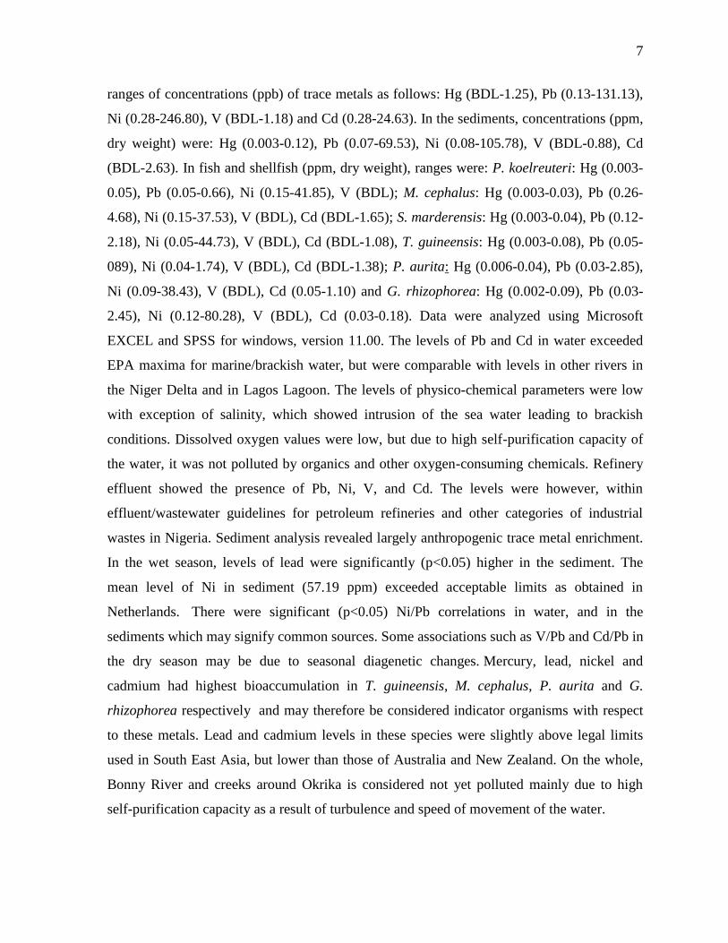
ranges of concentrations (ppb) of trace metals as follows: Hg (BDL-1.25), Pb (0.13-131.13),
Ni (0.28-246.80), V (BDL-1.18) and Cd (0.28-24.63). In the sediments, concentrations (ppm,
dry weight) were: Hg (0.003-0.12), Pb (0.07-69.53), Ni (0.08-105.78), V (BDL-0.88), Cd
(BDL-2.63). In fish and shellfish (ppm, dry weight), ranges were: P. koelreuteri: Hg (0.003-
0.05), Pb (0.05-0.66), Ni (0.15-41.85), V (BDL); M. cephalus: Hg (0.003-0.03), Pb (0.26-
4.68), Ni (0.15-37.53), V (BDL), Cd (BDL-1.65); S. marderensis: Hg (0.003-0.04), Pb (0.12-
2.18), Ni (0.05-44.73), V (BDL), Cd (BDL-1.08), T. guineensis: Hg (0.003-0.08), Pb (0.05-
089), Ni (0.04-1.74), V (BDL), Cd (BDL-1.38); P. aurita: Hg (0.006-0.04), Pb (0.03-2.85),
Ni (0.09-38.43), V (BDL), Cd (0.05-1.10) and G. rhizophorea: Hg (0.002-0.09), Pb (0.03-
2.45), Ni (0.12-80.28), V (BDL), Cd (0.03-0.18). Data were analyzed using Microsoft
EXCEL and SPSS for windows, version 11.00. The levels of Pb and Cd in water exceeded
EPA maxima for marine/brackish water, but were comparable with levels in other rivers in
the Niger Delta and in Lagos Lagoon. The levels of physico-chemical parameters were low
with exception of salinity, which showed intrusion of the sea water leading to brackish
conditions. Dissolved oxygen values were low, but due to high self-purification capacity of
the water, it was not polluted by organics and other oxygen-consuming chemicals. Refinery
effluent showed the presence of Pb, Ni, V, and Cd. The levels were however, within
effluent/wastewater guidelines for petroleum refineries and other categories of industrial
wastes in Nigeria. Sediment analysis revealed largely anthropogenic trace metal enrichment.
In the wet season, levels of lead were significantly (p<0.05) higher in the sediment. The
mean level of Ni in sediment (57.19 ppm) exceeded acceptable limits as obtained in
Netherlands. There were significant (p<0.05) Ni/Pb correlations in water, and in the
sediments which may signify common sources. Some associations such as V/Pb and Cd/Pb in
the dry season may be due to seasonal diagenetic changes. Mercury, lead, nickel and
cadmium had highest bioaccumulation in T. guineensis, M. cephalus, P. aurita and G.
rhizophorea respectively and may therefore be considered indicator organisms with respect
to these metals. Lead and cadmium levels in these species were slightly above legal limits
used in South East Asia, but lower than those of Australia and New Zealand. On the whole,
Bonny River and creeks around Okrika is considered not yet polluted mainly due to high
self-purification capacity as a result of turbulence and speed of movement of the water.

8
LIST OF FIGURES
Figure 3.1: Map of Bonny River and creeks in Rivers State, showing sampling
Stations 59
Figure 4.1: Seasonal mean levels of trace metals in water of Bonny River and
Creeks around Okrika. 75
Figure 4.2: Mean seasonal values of physico-chemical parameters in water of
Bonny River and creeks around Okrika. 83
Figure 4.3a: Two-monthly mean levels of trace metals in sediments of Bonny
River and creeks around Okrika. 89
Figure 4.3b: Two monthly mean levels of organic matter in sediments of Bonny
River and creeks around Okrika. 89
Figure 4.4: Mean levels of trace metals in shellfish and fish of Bonny River
and creeks around Okrika. 92
9
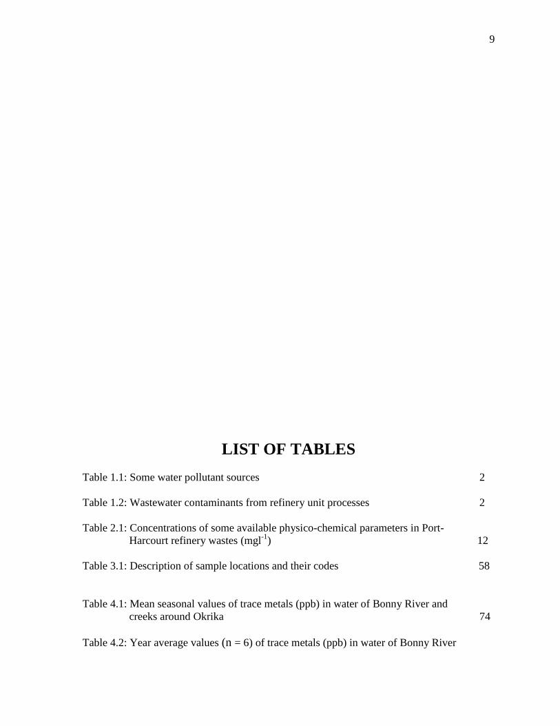
LIST OF TABLES
Table 1.1: Some water pollutant sources 2
Table 1.2: Wastewater contaminants from refinery unit processes 2
Table 2.1: Concentrations of some available physico-chemical parameters in Port-
Harcourt refinery wastes (mgl-1
) 12
Table 3.1: Description of sample locations and their codes 58
Table 4.1: Mean seasonal values of trace metals (ppb) in water of Bonny River and
creeks around Okrika 74
Table 4.2: Year average values (n = 6) of trace metals (ppb) in water of Bonny River

10
and creeks around Okrika 75
Table 4.3: Correlation matrices for the combined trace metal data of water from
Bonny River and creeks around Okrika 76
Table 4.4: Year average (n = 6) values of physico-chemical parameters (ppb, except
pH, temperature, conductivity and turbidity) in water of Bonny River and
creeks around Okrika in Rivers State, Nigeria 77
Table 4.5a: Mean levels of physico-chemical parameters in water of Bonny River and
creeks around Okrika in the dry season 78
Table 4.5b: Mean levels of physico-chemical parameters in water of Bonny River and
creeks around Okrika in the wet season 79
Table 4.6a: Correction matrices: Trace metals versus physico-chemical parameters in
the dry season 86
Table 4.6b: Correction matrices: Trace metals versus physico-chemical parameters in
the wet season 86
Table 4.7: Year average (n = 6) values (ppm, dry weight.) of parameters in
sediments of Bonny River and creeks around Okrika
87
Table 4.8: Levels of trace metals (ppm, dry weight) in sediments of Bonny River
and creeks around Okrika compared with Netherlands class limits
sediment with organic matter content >10%
88
Table 4.9: Mean seasonal values of parameters (ppm, dry weight.) in sediments of
Bonny River and creeks around Okrika 88
Table 4.10a: Correction matrices of trace metals and organic matter in sediments of
Bonny River and creeks around Okrika for dry season 90
Table 4.10b: Correction matrices of trace metals and organic matter in sediments of
Bonny River and creeks around Okrika for wet season 90
Table 4.11: Trace metal levels (ppb) in refinery effluent/wastewater compared with
Effluent/wastewater limitation guidelines in Nigeria 91
Table 4.12: Mean levels (ppm) of trace metals in shellfish and fish (dry weight) of Bonny
River and creeks around Okrika
91

11
Table 4.13: Bio-accumulation factor (BF) for trace metals in muscle tissues of shell-
fish and fish from Bonny River and creeks around Okrika 93
Table 4.14: Ranges of trace metals (ppm, fresh weight) for fish of Bonny River and
those of Niger Delta, Lagos Lagoon and Central Africa 93
Table 4.15: Limits of some trace metals in shellfish and fish acceptable in some
countries compared with mean levels of same metals in Bonny
River and creeks around Okrika
94
Table 4.16: Trace metal levels (ppb) in water of Bonny River and creeks around
Okrika, Niger Delta and Lagos Lagoon in ranges
98
Table 4.17: US EPA maximum allowable levels in water compared with levels in
Bonny River and creeks around Okrika 98
TABLE OF CONTENTS TITLE PAGE……………………………………………………………………….................i

12
APPROVAL PAGE…………………………………………………………………………..ii
CERTIFICATION……………………………………………………………………………iii
DEDICATION……………………………………………………………………..................iv
ACKNOWLEDGEMENT…………………………………………………………………….v
ABSTRACT…………………………………………………………………………………..v
i
LIST OF FIGURES…………………………………………………………………………viii
LIST OF TABLES………………………………………………………………....................ix
TABLE OF CONTENTS……………………………………………………………………..xi
CHAPTER ONE
INTRODUCTION
1.1: Oil industry and pollution in the Niger Delta 1
1.2: Significance/relevance of study 3
1.3: Aims and objectives 4
CHAPTER TWO
LITERATURE REVIEW
2.1: Environmental pollution monitoring 5
2.2: Pollution studies in aquatic systems 6
2.2.1: The surface water medium 6
2.2.2: The sediments 6
2.2.3: The biota 7
2.3: Effects of oil spills and direct discharge of refinery wastes into the aquatic
system 7
2.4: Oil pollution and the aquatic organisms 9
2.5: Point and diffuse sources of waste discharge
10
2.6: Treatment of liquid effluent 11
2.7: Sources and accumulation of trace metals 12

13
2.8: Some environmental consequences of trace metals 14
2.8.1: The Surface water 14
2.8.2: The associated sediments 15
2.8.3: The aquatic organisms
16
2.9: Toxicological potential of trace metals 18
2.9.1: Toxicity of mercury, cadmium, lead, vanadium, and nickel
18
2.9.2: Effects of toxicity of some of the trace metals and others on marine
Organisms 26
2.10: Reviews of some physio-chemical parameters in water 30
2.10.1: Nutrients in the aquatic ecosystem
38
2.10.2: Major cations
41
2.11: Sediments pollution in the aquatic ecosystem
42
2.11.1: Sediment organic matter 45
2.12: Analytical techniques for trace metals analysis of environmental
Samples 46
2.12.1: Detection techniques for trace metals in environmental samples 47
2.12.2: Sampling and sample preservation 49
2.12.2.1: Sampling and storage of sediments 50
2.12.2.2: Sampling and storage of water 50
2.12.2.3: Collection of biological samples 52
2.12.3: Sample preparation for trace metals determination by atomic absorption
spectrophotometry 52
2.12.3.1: Extraction of trace metals from sediments 52
2.12.3.2: Extraction of trace metals from water 54
2.12.3.3: Extraction of metals from biological materials 55

14
CHAPTER THREE
METHODOLOGY
3.1: Description of study area 57
3.1.1: Description of sample locations 58
3.2: Materials and methods 60
3.2.1: Collection of surface water samples 60
3.2.2: Collection of sediments samples 61
3.2.3: Collection of shellfish and fish samples 61
3.2.4: Collection of effluent/wastewater samples 61
3.3: Preparation of stock solutions 62
3.4: Sample treatment and analysis 62
3.4.1: Determination of trace metals in sediments 62
3.4.1.1: Determination of mercury-Cold vapour technique 62
3.4.2: Determination of total organic carbon (TOC) and total organic matter (TOM)
in sediments
63
3.4.3: Determination of trace metals in water 64
3.4.4: Determination of major cations in water
65
3.4.5: Determination of trace metal in effluent/wastewater 65
3.4.6: Determination of water quality and nutrients components 66
3.4.6.1: Determination of pH (electrometric method) 66
3.4.6.2: Determination of temperature 66
3.4.6.3: Determination of total dissolved solids (TDS) 67
3.4.6.4: Determination of salinity 67
3.4.6.5: Determination of electrical conductivity 67
3.4.6.6: Determination of total hardness by complexometric titration 67
3.4.6.7: Determination of total alkalinity by titrimetry 68
3.4.6.8: Determination of dissolved oxygen (DO) by the winkler’s method 68
3.4.6.9: Determination of biological oxygen demand (BOD5) 68
3.4.6.10: Determination of chemical oxygen demand (COD) 69

15
3.4.6.11: Determination of silicates 69
3.4.6.12: Determination of water turbidity 70
3.4.6.13: Determination of total suspended solids (TSS) 70
3.4.6.14: Determination of sulphate ion (SO42-
) – Turbidimetric method 70
3.4.6.15: Determination of nitrate ion (NO3-) – Colorimetric method 71
3.4.6.16: Determination of phosphate ion (PO43-
) – Stannous chloride method 71
3.4.7: Shellfish and fish 72
3.4.7.1: Determination of trace metals in shellfish 72
3.4.7.2: Determination of trace metals in fish 72
3.5: Quality assurance for trace metals analysis 73
3.6: Statistical analysis of data 73
CHAPTER FOUR
RESULTS AND DISCUSSION
4.1: Results of water analysis 74
4.2: Results of sediments analysis 87
4.3: Results of refinery effluent/wastewater analysis 90
4.4: Results of shellfish and fish analysis 91
4.5: Discussion 94
4.5.1: Trace metals in water and sediment 95
4.5.2: Trace metals in shellfish and fish
99
4.5.3: Conclusion
101
4.5.4: Contributions to knowledge 102
4.5.5: Recommendation
103

16
REFERENCES 104
Appendices
17
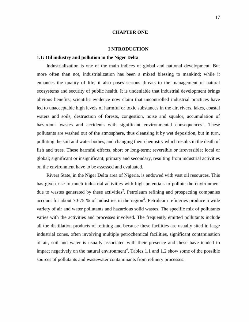
CHAPTER ONE
I NTRODUCTION
1.1: Oil industry and pollution in the Niger Delta
Industrialization is one of the main indices of global and national development. But
more often than not, industrialization has been a mixed blessing to mankind; while it
enhances the quality of life, it also poses serious threats to the management of natural
ecosystems and security of public health. It is undeniable that industrial development brings
obvious benefits; scientific evidence now claim that uncontrolled industrial practices have
led to unacceptable high levels of harmful or toxic substances in the air, rivers, lakes, coastal
waters and soils, destruction of forests, congestion, noise and squalor, accumulation of
hazardous wastes and accidents with significant environmental consequences1. These
pollutants are washed out of the atmosphere, thus cleansing it by wet deposition, but in turn,
polluting the soil and water bodies, and changing their chemistry which results in the death of
fish and trees. These harmful effects, short or long-term; reversible or irreversible; local or
global; significant or insignificant; primary and secondary, resulting from industrial activities
on the environment have to be assessed and evaluated.
Rivers State, in the Niger Delta area of Nigeria, is endowed with vast oil resources. This
has given rise to much industrial activities with high potentials to pollute the environment
due to wastes generated by these activities2. Petroleum refining and prospecting companies
account for about 70-75 % of industries in the region3. Petroleum refineries produce a wide
variety of air and water pollutants and hazardous solid wastes. The specific mix of pollutants
varies with the activities and processes involved. The frequently emitted pollutants include
all the distillation products of refining and because these facilities are usually sited in large
industrial zones, often involving multiple petrochemical facilities, significant contamination
of air, soil and water is usually associated with their presence and these have tended to
impact negatively on the natural environment4. Tables 1.1 and 1.2 show some of the possible
sources of pollutants and wastewater contaminants from refinery processes.

18
Table 1.1 Some water pollutant sources1
Pollutants Sources
BOD, COD, Oil, total suspended solids (TSS)
Process wastewater, cooling tower (if hydrocarbons leak into cooling water systems), ballast water, tank flow drainage and run-offs. Process wastewater, rank flow drainage and run-offs.
Total suspended solids (TSS)
Process wastewater, cooling tower blow down, ballast water, tank flow drainage and runoffs.
Phenolics
Process wastewater (particularly from the fluid catalytic cracking unit).
NH3, H2S, trace organics
Process wastewater (Particularly from the fluid catalytic) cracking unit and coker).
Heavy metals
Process wastewater, tankage wastewater discharges, cooling tower blow down (if chromate type cooling water treatment chemicals are used)
Table 1.2 Wastewater contaminants from refinery unit processes
1
Processes
Wastewater
Pollutants typically expected in waste- water
Crude oil desalting
Yes
Inorganic chlorides, HC, (H2S, Phenols), SS
Atmospheric distillation Yes HC, H2S.(NH3, Phenols)
Vacuum distillation Yes HC, H2S. (NH3, Phenols)
Fluid catalytic cracking Yes HC, H2S, NH3, CN Phenols
Coking (delayed or fluid) Yes HC, H2S, NH3, CN, Phenols
Visbreaking Yes HC, H2S, NH3, CN, Phenols
Steam cracking (gas oils) Yes HC, H2S, NH3, CN, Phenols
Catalytic hydro cracking Yes H2S, NH3, (HC), Phenols
Catalytic reforming Yes H2S, HCl
Naphtha hydrodesulphurization
Yes
H2S, NH3, HC, (Phenols)
Distillate Hydrodesulphurization
Yes
H2S, NH3, HC, (Phenols)
Heavy oil Hydrodesulphurization
Yes
H2S, NH3, HC, (Phenols)
Gas recovery plants: unsaturates saturates
Yes Yes
H2S, NH3, RSH, CN, amine, (HC Phenols) H2S, NH3, RSH, CN, amine, (HC)
Merox treaters Yes NaSH, NaSR Sodium Phenolates, (HC)
Alkylation Yes Sulphuric or hydrofluoric acid or acid salts, SS
Isomerization Yes Caustic stream containing organic chlorides
Hydrogen synthesis Yes (CO2, CN, NH3, amine)
Aromatics extraction Yes (Solvents, aromatics, HC)
Petrochemicals Yes (Various)
Lubricating Yes Solvents and various others
Asphalt Yes HC, (Phenols)
Sulphur recovery No * RSH- Mercaptans, NaSR- sodium mercaptides, NaSH- sodium hydrosulphide
* The pollutants in ( ) indicate those which may not be present in all cases.

19
Other sources of pollutants in the Niger Delta area include: jetty activities, household wastes,
those from other industries such as Dangote cement factory, Notore Chemical Industries
Limited (formally National Fertilizer Company of Nigeria (NAFCON)), DAEWOO
Construction Company, dredging activities of B+B and HAM dredging companies and
marine transport.
1.2: Significance/relevance of the study
Apart from the effects of the oil industries, other human activities resulting in dumping
of domestic, agricultural and industrial wastes into the environment are very prominent in
Okrika and environs. The area hosts the Port Harcourt Refining Company (PHRC), amidst
exploration and exploitation activities. Because these facilities often involve multiple
industrial processes, significant contamination of air, soil and water is usually the
consequence. Residents of adjourning communities are potentially at risk from the inhalation
of polluted air and drinking of polluted water. Large volumes of hazardous wastes are
generated and released into the environment. Such hazardous wastes, among others, are trace
metals, which ultimately find their way into natural water bodies, the natural habitats of fish5
and bioaccumulate in sediments and sedentary organisms such as periwinkle, polychaetes,
etc.
The study area represents a reasonable percentage within the oil-producing area. Before
now, Bonny River and creeks around Okrika, not only serve for thriving fishing and other
economic activities, but also a source of fresh water for domestic purposes during ebb tides.
However, the water is now vulnerable to oil pollution and much of the fishing and other
activities apart from purely industrial ones have been reduced. Moreover, this area consists of
many productive river systems, creeks, shorelines, fresh water, mangrove swamps and sandy
beaches. The Port Harcourt Refining Company (PHRC), Pipelines Product Marketing
Company (PPMC), Daewoo Notore Chemical Industries Limited (formally NAFCON) and a
whole lot of industrial activities depend on these creeks and rivers for communication and
discharge of wastes and effluents (either untreated or given only primary treatment). Marine
activities, such as speed boat transport services are also remarkable. Oil spillage is one of the
most serious environmental hazards linked with oil exploitation in the Niger Delta region of
Nigeria. Oil exploration and exploitation activities have led to the development of associated

20
industries such as refineries, petrochemical, and fertilizer plants3, 6-7
. It has been observed
that untreated effluents are often dumped directly into the creeks, and rivers such as Bonny
and Warri Rivers and the Atlantic Ocean. These untreated effluents are hazardous to both
terrestrial and aquatic environments. This exactly depicts the state of the oil industry in the
Niger Delta area of Nigeria.
The continuous exposure of the area to wastes from the above activities, among others,
may have had some negative impacts. It is suspected that fish and sediments feeders like
periwinkles may have been highly contaminated with trace metals and other toxic chemicals,
hence endangering the health of those who consume them. It is on the basis of the above, that
it became necessary to assess the river water quality, and pollution status of Bonny River and
creeks around Okrika.
1.3: Aims and objectives
The objectives of this study include:
1. to characterize the water of Bonny River and the creeks in Okrika area;
2. to assess the quality of Bonny River and the creeks around Okrika;
3. to determine trace metals: Hg, Pb, Ni, V and Cd in water, sediment and biota in Bonny River and
creeks in Okrika with the following aims:
(a) to identify possible pollutants and their likely sources;
(b) to assess bioaccumulation of each metal in the fish and shellfish analysed, and possibly identify
indicator species which can be used to monitor trace metal pollution of the ecosystem and
similar ones;
(c) to investigate the relationship, if any, between trace metal levels and nutrient levels in water;
(d) to describe any seasonal variabilities in trace metal levels and their dynamics in the different
matrices of the system,
(e) to evaluate the seasonal influence on the aquatic system, and
(f) to contribute to baseline data on trace metal levels and other pollutants in the area in
particular, and Nigerian in general.

21
CHAPTER TWO
LITERATURE REVIEW
2.1: Environmental pollution monitoring
Environmental pollution monitoring programmes are developed in relations to problems
of increasing gross and site-specific pollution in the environment8. In some instances, there
were warnings that specific pollutants should be measured periodically in the bid to evaluate
their impacts. In other cases, recommendations have suggested that it is important to monitor
pollutants in water, sediments, as well as the body burden of contaminants in key or sentinel
biota. Environmental pollution monitoring has therefore been considered to consist of
repetitive data collection for the purpose of determining trends in environmental parameters9.
Assessments which are possible through monitoring include both a priori indications of
problems developing in a resource before such problem becomes critical, and a posteriori
evaluation of temporal change in particular parameter of interest.
Numerous reasons for conducting environmental evaluation and monitoring have been
recognized10-11
. These reasons include among others:
- to screen effluents, receiving water and biota or potentially harmful toxicants,
including in certain cases, the assessment of requirements for emission
control;
- to investigate the effect of environmental quality on human health or other
parameters, in an attempt to elucidate cause and effect relationship;
- to study the sources, transport pathways and sinks for contaminants in the
environment;
- to provide a historic record of emission or of environmental quality, in order
to ascertain compliance rates with relevant standards or legislation;
- To investigate the specific environmental impact of individual pollutants.
Studies may be undertaken in product evaluation, or in attempts to minimize the
detrimental impacts of effluents/emissions on ecosystems or in investigation such as hazard
assessment. Binning and Baird12
studied the Swartkops River ecosystems to determine the
source of pollutants (trace metals) so that their concentrations do not get to toxic levels.

22
2.2: Pollution studies in aquatic systems
Various environmental segments are analyzed to assess, monitor and control aquatic
pollution. The major reasons for the particular sensitivity of aquatic systems to pollution
influences may lie in the structure of their food chain compared with land systems; the
relatively small biomass in the aquatic environments generally occur in a greater variety of
trophic levels, whereby accumulation of toxic substances can be enhanced. It is therefore
now recognized that no country can afford to ignore the sound arrangement and protection of
her environment and resources, which form the basis for development13
.
2.2.1: The surface water medium
The most obvious medium is surface water14
. However, it has been established that
concentrations of most contaminants of concern in either fresh water or salt waters are very
low ranging from around the nanogram per litre (parts per trillion or 1012
) level to about the
milligram per litre (parts per million) level depending on the contaminants involved. This,
not only renders the analyses of such waters technically difficult, but may also introduce
inadvertent errors in sample collection and analytical procedures15
.
Furthermore, quantification of contaminants in natural waters suffers from additional
disadvantages with respect to its use as a regular monitoring tool. Accordingly, the
concentrations of contaminants in a given environment vary widely with time. Forstner and
Wittmann14
attributed such fluctuations to a large number of variables, such as daily and
seasonal variations in water flow, surreptitious local discharges of effluents, changing pH and
redox conditions, the input of treated secondary sewage, detergent levels, salinity and
temperature. Perhaps, the greatest disadvantage of the analysis of natural water, for
contaminants is the lack of any useful connection between the concentrations of
contaminants in the system and their biological availability.
2.2.2: The sediment
Owing to difficulties associated with trace determinations in surface water, many have
employed sediments to monitor the contamination of the aquatic environments14
. Most
contaminants of concern in aquatic ecosystems have a propensity to associate preferentially
with suspended particulate matter rather than being maintained in solution, although this
behaviour varies to an extent between individual contaminants.

23
Philip and Rambow15
however, identified two major problems associated with any
reliance upon sediments for monitoring contaminants in aquatic ecosystems. Firstly,
concentrations of contaminants in sediment do not reflect the absolute magnitude of
contaminants’ abundance at the sampling point. Secondly, concentrations of contaminants
are affected by grain size and organic carbon content.
2.2.3: The biota
Aquatic organisms have also long been known to accumulate significant quantities of
some contaminants in their tissues. This accumulation and sequestration of contaminants by
organisms provide an opportunity to short-circuit the traditional methods of monitoring
pollution in aquatic environments through the analysis of water. This is by employing
organisms for such monitoring. In the USA, a bivalve mollusk has been used in a national
programme to monitor pesticides in estuaries16
. The greatest advantage of the use of such
bio-monitors is that the bioavailability of the pollutant is measured directly without recourse
to the assumptions employed in the other two methods thus; a contaminant present in the
organism is by this definition, bio-available.
2.3: Effects of oil spills and direct discharge of refinery wastes into the aquatic system
Crude oil is a mixture of many thousands of organic compounds, more than three
quarter of which is usually hydrocarbons. Other constituents in trace concentrations are
Sulphur-Oxygen-Nitrogen containing compounds and some trace metals, particularly nickel
and vanadium17
. Crude oil is a dark-brown viscous liquid, which is less dense than seawater.
Oils are generally classified as either crude oil or refined products or according to their
viscosity. Crude oils contain similar molecular species with thousands of compounds ranging
from gases to residues with boiling points above 35ºC and they vary markedly in detailed
composition.
According to Odu18
, Nigerian crude oils are basically of two types. These are the
Nigerian light, which contain a high percentage of naphthenic hydrocarbons, and the
Nigerian medium, which has a higher specific gravity and more residues boiling at
temperature above 37ºC.

24
Nwankwo and Irrechukwu19
identified several sources from which oil may spill and
cause pollution in Nigeria’s Niger Delta. These are:
(i) Onshore and offshore exploration and production;
(ii) Transportation operations;
(iii) Marketing operations, including terminal operations;
(iv) Petroleum refining
These sources were further reviewed by Ifeadi and Nwankwo20
and Oyefolu and Awobayo21
,
who identified flow line/pipeline leaks, overpressure failures/overflow of process equipment
components, sabotage to well heads and flow lines, hose failures on the SBM/SPM tanker
loading system and failure along pump discharge manifolds (vibration effects) as the main
causes of oil pollution in the Niger Delta.
Sequel to oil spillages, the activities of oil industries and the discharge of wastes into the
aquatic environment, large areas of tropical sea, coral reefs and flats, sea grass beds,
mangrove swamps and intertidal flats are potentially at risk22
. Oil can harm aquatic life
directly or indirectly by reducing the amount of light that enters the water. This was the
observation of Effiong4, who reported that this could prevent natural aeration and lead to
death of aquatic organisms trapped below it. Powell23
, on his part, further stated that fish may
ingest the spilled oil resulting in fish mortalities. For this reason, fish even when caught alive
for consumption are often unpalatable. These view had been corroborated by Pickering and
Owen24
, who reported that industrial activities pollute the air, water and soil, and over time,
pollutants accumulate across tropic levels to pose serious health hazards to man as they find
their way into the food chain, albeit in small doses.
The risk of contamination of natural water bodies, the ultimate recipient of all forms of
pollutant has been evaluated as significant. This is because when these pollutants get into the
aquatic system, they are distributed and partitioned into different components of the marine
ecosystem (water, sediment, flora and fauna), which is regulated by physiochemical
processes such as dilution, diffusion, precipitation and sorption, as well as uptake and
elimination. These pollutants (in most cases, metals) are rapidly absorbed by particulate
materials (detritus, plankton, suspended sediments, etc) and assimilated by living organisms.
Eutrophication, among others, of lakes and rivers is an inevitable consequence, and this

25
progresses rapidly due to increase in organic substances and nutrient salts causing unusual
growth of specific organisms, thus destroying the normal aquatic system.
2.4: Oil pollution and the aquatic organisms
Oil spillage effects and the ecological impacts are influenced by a number of factors
such as: the quantity of oil impacting the environment; the type of oil; metrological
conditions; turbidity of the water; the pressure of other pollutants; the effects of seasonal
changes; the type of biota and treatment of spills25
. The biological systems found to be
directly impacted by crude oil include mammals, birds, reptiles, fish, crustaceans, mollusks,
polychaetes, zooplankton, phytoplankton25
as reported by Ekweozor26
.
Oil pollution, whether it is due to spillage or the discharge of crude oil or refined
products, may damage the aquatic ecosystem in a number of ways. These include:
- Direct kill of organisms through coating and asphyxiation;
- Direct kill of organisms through contact poisoning of organisms;
- Direct kill of organisms through exposure to water soluble toxic components
of some distance in time space from the spill site;
- Destruction of the generally more sensitive juvenile forms of organisms;
- Destruction of food sources of higher species;
- Incorporation of sub-lethal amounts of oil and oil products into organisms,
resulting in reduced resistance to infection and other stresses;
- Destruction of food values through the incorporation of oil and oil products
into the aquatic environment and incorporation of carcinogens into the marine
food chain and human food sources;
- Low-level effects that may interrupt any of the numerous events necessary for
the propagation of marine species and for the survival of these species, which
are in the aquatic food chain17, 26
.
A major concern of oil spillages is their effect on fish and fisheries. This is often given
as a prime justification for the obvious toxicity and spillage impact studies sponsored by oil
companies and regulatory bodies. Unfortunately, most are not publicly available23
. The
author further stated that there is good evidence of local fisheries being affected by avoidance
of other areas by migrating fish.

26
During their studies on the establishment of baseline data for complete monitoring of
petroleum related aquatic pollution in Nigeria, Ibiebele et. al.27
identified three major aquatic
zones of oil producing area of Nigeria. These include:
- Non-tidal freshwater swamps
- Tidal freshwater swamps
- Mangrove (saline) swamps
They reported that oil fields, pipelines and oil spill figures are more in the freshwater zones
than in the mangrove survey zones in the Niger Delta. They further stated that pollution
events within freshwater swamps are likely to have severe but localized effects, except where
and when watercourses and water levels are such as to spread the pollutant.
2.5: Point and diffuse sources of waste discharge
Apart from oil spillage and its attendant problems, there are also outfalls of effluent
discharges from sewers, gutters, plants, drains and factories. These constitute the point
sources of waste discharge. Most cases of accidentals, negligent or illegal discharges are also
from point sources. The concentration of pollutants in the receiving water bodies is initially
high, decreasing as the distance from the point source increases28
.
Some of the more serious forms of pollution arise however, from diffuse sources that is,
the pollutants are discharged into the water from sources other than a single point source. For
example, in agricultural areas, surface water bodies, agricultural land drainage, surface run-
off, underground water infiltration into lakes and rivers, can introduce plant nutrients (from
fertilizers) and pesticides in substantial quantities into water bodies. The effect of pollution
from such diffuse sources can be serious too.
Most effluents are complex mixtures of a large number of different harmful agents.
These include toxic substances of many kinds, high levels of suspended solids, and dissolved
and particulate putrescible organic matter. In addition, effluents from thermal plants could be
hot with high pH values, and could contain high levels of dissolved salts. If the cooling water
from a power plant is discharged at a raised temperature into rivers, it may increase the
temperature of the water bodies up to 40 ºC. Such temperature may completely eliminate fish
in the river. Elevated temperatures have a number of effects on the water body. Density and
viscosity are decreased, permitting suspended solids to settle at a faster rate; evaporation,

27
rate of chemical reactions also increase. This could lead to fast assimilation of waste and
faster depletion of dissolved oxygen29
.
2.6: Treatment of liquid effluent
Refinery wastewaters often require a combination of treatment methods to remove oil
and other contaminants before discharge1. Separation of different streams (such as
stormwater) is essential to minimize treatment requirements. Oil is recovered using
separation techniques. For heavy metals, a combination of oxidation/reduction, precipitation,
and filtration is used. For organics, a combination of air or steam stripping, granular
activated carbon, wet oxidation, ion exchange, reverse osmosis, and electrodialysis is used.
A typical system may include neutralization, coagulation/flocculation,
flotation/sedimentation/filtration, biodegradation (trickling filter, anaerobic, aerated lagoon,
rotating biological contactor, and activated sludge), and clarification. A final polishing step
using filtration, ozonation, activated carbon, or chemical treatment may also be required.
Some pollutants loads, among other which may be found in the Port Harcourt refinery
effluent/wastewater are given in Table 2.1 below.
28
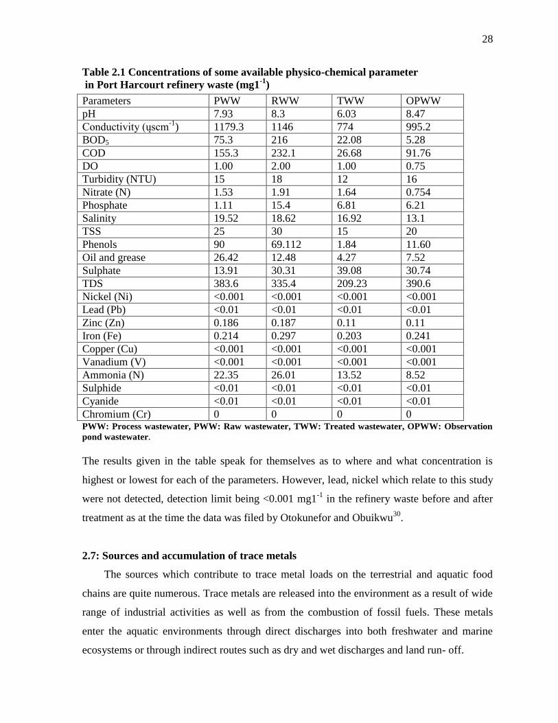
Table 2.1 Concentrations of some available physico-chemical parameter
in Port Harcourt refinery waste (mg1-1
)
Parameters PWW RWW TWW OPWW
pH 7.93 8.3 6.03 8.47
Conductivity (ųscm-1
) 1179.3 1146 774 995.2
BOD5 75.3 216 22.08 5.28
COD 155.3 232.1 26.68 91.76
DO 1.00 2.00 1.00 0.75
Turbidity (NTU) 15 18 12 16
Nitrate (N) 1.53 1.91 1.64 0.754
Phosphate 1.11 15.4 6.81 6.21
Salinity 19.52 18.62 16.92 13.1
TSS 25 30 15 20
Phenols 90 69.112 1.84 11.60
Oil and grease 26.42 12.48 4.27 7.52
Sulphate 13.91 30.31 39.08 30.74
TDS 383.6 335.4 209.23 390.6
Nickel (Ni) <0.001 <0.001 <0.001 <0.001
Lead (Pb) <0.01 <0.01 <0.01 <0.01
Zinc (Zn) 0.186 0.187 0.11 0.11
Iron (Fe) 0.214 0.297 0.203 0.241
Copper (Cu) <0.001 <0.001 <0.001 <0.001
Vanadium (V) <0.001 <0.001 <0.001 <0.001
Ammonia (N) 22.35 26.01 13.52 8.52
Sulphide <0.01 <0.01 <0.01 <0.01
Cyanide <0.01 <0.01 <0.01 <0.01
Chromium (Cr) 0 0 0 0 PWW: Process wastewater, PWW: Raw wastewater, TWW: Treated wastewater, OPWW: Observation
pond wastewater.
The results given in the table speak for themselves as to where and what concentration is
highest or lowest for each of the parameters. However, lead, nickel which relate to this study
were not detected, detection limit being <0.001 mg1-1
in the refinery waste before and after
treatment as at the time the data was filed by Otokunefor and Obuikwu30
.
2.7: Sources and accumulation of trace metals
The sources which contribute to trace metal loads on the terrestrial and aquatic food
chains are quite numerous. Trace metals are released into the environment as a result of wide
range of industrial activities as well as from the combustion of fossil fuels. These metals
enter the aquatic environments through direct discharges into both freshwater and marine
ecosystems or through indirect routes such as dry and wet discharges and land run- off.
29
In assessing such metal loads in some environmental segments, Ndiokwerre31
used
neutron activation analysis and atomic absorption spectrophotometry in the determination of
As, Au, Cd, Hg, Mn, Ni, Pb, Sb, and Zn in sediments and algae from River Niger and the
Nigerian Atlantic Coastal waters. The measured concentrations of As, Cd, Hg, and Sb were
higher in sediments from the coastal waters than sediments from River Niger. The sediments
from River Niger returned higher Mn, Pb and Zn concentrations, similar trends were also
observed in the algae. In addition to providing sinks for many harmful chemicals, sediments
have been identified to serve as potential sources of pollutants (especially metals) to the
water column when conditions in the receiving water system change (e.g. during periods of
anoxia, after severe storms) as well as highlight the integrated picture of the events taking
place in the water column12
.
Kokovides et. al.32
, in their study of the marinas, identified trace metal content
originating from metal corrosion, paint dissolution, fuel metal additives etc. as major factor
of pollution in the area. Investigations on the aquatic environment in Sweden revealed
abnormally high concentrations of mercury compounds in fresh and salt water fish and other
aquatic organisms. The source of mercury pollution was traced to discharge of mercurial
fungicides by a Paper Mill. Similarly, cadmium pollution of the Jintsu River, Japan was
attributed to zinc mine owned by Akiako and situated some 50m upstream from the affected
villages33
.
In a study carried out by Ibok et. al.34
on trace metals in fishes from some streams in
Ikot Ekpene area of Nigeria, zinc and lead levels in Qua Iboe River were noted to be high.
The authors attributed the high metal levels to both domestic sewage and drainage from
automobile workshops as well as effluents from Sunshine Batteries Industry in the area. They
further attributed the relatively high levels of cadmium, cobalt and lead to their presence in
run off waters, which may contain among other materials, paint waste containing pigments
from spraying workshops new or renovated buildings.
In the Niger Delta region, the petroleum industry is a major source of trace metals.
Crude oil contains widely varying concentrations of trace metals such as V, Ni, Fe, Al, Na,
Cu and U35
. Metals such as cadmium, barium, lead, copper, vanadium, iron and mercury are
commonly found in wastes generated from production operations in the petroleum industry29
.
World Bank36
had reported that, of the 5,500 tons of waste produced per year in River State

30
then, the Petroleum Industry generated more, thus exposing the rivers and creeks in these
areas to risk of contamination from petroleum and associated pollutants. There have been
reported incidences of oil spillages and seepage in addition to gas flaring in the area37-38
.
These spillages have the potential of introducing heavy metals and mineral hydrocarbons into
aquo-terrestrial environments which ultimately settle into sediment matrices39
. Also, air-
borne particulates derived from fossil fuel combustion also contain trace (heavy) metals40
.
These pollutants are potentially deleterious to aquatic plants and animals and as well devalue
the integrity of water bodies.
2.8: Some environmental consequences of trace metals
The problems associated with trace metals contamination were first highlighted in
industrial discharges and especially by the incidents of mercury and cadmium pollution in
Sweden and Japan41
. The likely major source of most of these chemicals is the industrial
waste being added to city sewage system.
Environmental contamination from trace metals is of global concern because it exhibits
behaviour consistent with those of persistent toxic chemicals. Unlike many organic
contaminants, that lose toxicity with biodegradation, metals cannot be degraded further and
their toxic effect can be long lasting42
, while the concentrations in biota can be increased
through bioaccumulation. Moreso, trace metals, even at low concentrations are known to
have toxic effects43
.
2.8.1: The surface water
Studies have shown that many water bodies in Nigeria contain various levels of trace
metals pollutants44-47
. Further studies on the River Niger have also implicated the tributaries
as contributors to the heavy metal load48
. More so, large quantities of contaminants including
heavy metals in surface water have been widely reported44-45, 49
, as arising from the discharge
of industrial and domestic wastes into rivers, lakes and estuaries, especially those running
through major commercial cities. Estuaries occupy unique ecological niche. They are areas of
increased biological activity and are potential nursery grounds for many commercial fish
species. Metals normally enter the estuarine environment via rivers through normal
weathering and erosion processes. Trace metals occur as natural constituents of the marine

31
environment at low concentrations, and are capable of exerting considerable biological
effects at such levels.
Natural water is said to be polluted once it has been rendered unfit for use by human or
natural activities; and any substance that prevents the normal use of water is said to be a
water pollutant. Heavy metals, and in particular, those in the first row of the transition
elements including Cr, Mn, Fe, Co, Ni, Zn and Cu, are natural constituents of sediments. The
concentrations of these metals in river sediments reflect the occurrence and abundance of
certain rocks or mineralized deposits in the drainage area of the river50
. Disposal of sewage
into the water can be hazardous. Apart from the bacteriological contamination, sludge often
contains appreciable amounts of trace metals such as Zn, Cu, Ni, Cd, Fe and Pb. These
metals produce unhealthy effects at the threshold doses of various aquatic fauna and flora51
.
2.8.2: The associated sediment
There had been a comprehensive review of trace metals in waters and sediments of
rivers including Ogunpa and Ona Rivers in Ibadan, Okrika River, Warri River, Lagos lagoon,
Osun River in Oshogbo, Asa and Oyin Rivers in Ilorin and Kaduna River, all in Nigeria52
.
The trace metal concentrations were found to depend on industrial and human – related
activities such as petroleum exploration and exploitation, mining, industrial wastes and
vehicular emissions. Studies carried out previously showed relationship of high
concentrations of trace metals such as Cd, Pb, Cu, Ni, Mn and Co in some rivers with
proximity to industrial cities in Nigeria52
. These previous studies among others, have in fact,
informed the present study on rivers and creeks in Okrika area including the Bonny River.
Trace metals in sediments can play a major role in the pollution scheme of a river
system. Sediments are repositories for physical debris and sink for contaminants. They can
therefore be used to detect pollutants that escape water analysis and also provide information
about the critical sites of the river system14
. Andren53
reported that 67 % of Mercury in
Mississippi River is associated with suspended sediments. The fate of Hg and Cd considered
among the most toxic metals was investigated in the sediments from the Calabar River
estuary54
. It was a 60 km long estuary flowing under equatorial climate and characterized by
seasonal variation of fluxes of floral suspended matter that can be classified as a mesotidal

32
system. Previous studies had provided a fair knowledge of the major hydrodynamic
processes in estuaries. For example, Benson and Etesin55
reported that the river flows from
800 to 3000 m3s
-1. Because of variation of the hydrodynamic conditions, and also their longer
residence time in the sediment compared to suspended matter, Hg and Cd were studied in the
sediments.
2.8.3: The aquatic organisms
Ecological perturbation and bioaccumulation in aquatic organisms arising from riverine
discharges through on and offshore crude oil exploitation activities have also been
reported55, 56-58
. Information from a variety of sources indicates that sediments and fauna in
aquatic ecosystems throughout the Niger Delta are contaminated by a wide range of toxic and
bioaccumulative substances including metals, mineral hydrocarbons, etc22, 59-61
.
Aquatic organisms bio-accumulate trace metals in considerable amounts62-63
. It has been
reported for instance, that, in the flat oysters Ostrea edulis, individuals originating from a
clean area were able to accumulate Cd twice as fast as oysters living in a Cd contaminated
area, a fact which could result from an increased resistance in oysters chronically exposed to
the metal in their natural environment64
.
The bioaccumulation of Cd, Pb and Hg in the muscles, kidney and liver of nine (9) fish
species collected from the Warri Rivers has also been examined65
. The results showed
significant differences at p<0.05 in the accumulation of these metals in the muscles and the
other organs of the fish species. The accumulation pattern of lead in the liver of the species
was generally higher in the area which receives the refinery effluents being discharged into
the river.
Lowe et. al.66
found that freshwater fish collected from rivers in the USA had mean
levels of cadmium as follows: 1978 (0.04 ppm); 1979 (range: 0.01-0.41 ppm); 1980 (0.03
ppm) and 1981 (range: 0.01 – 0.35 ppm). On the other hand, lead was detected at mean levels
of 0.19 ppm in 1978 and 1979, and 0.17 ppm in 1980 and 1981. Similarly, Obasohan and
Oransaye67
found that freshwater fish collected from Ogba river in Nigeria had mean levels
of cadmium as follows: 0.074 ± 0.13 mgkg-1
for Oreochromis niloticus; 0.07 ± 0.15 mgkg-1
for Hemichromis fasciatus, and lead: 2.67 ± 4.00 mgkg-1
for O. niloticus and
2.00 ± 2.67 mgkg-1
Pb for H. fasciatus.
33
Fish are often at the top of aquatic food chain and may concentrate large amounts of
some trace metals. Accumulation pattern of contaminants in fish depends on both uptake and
elimination rate68-69
. Studies have shown that fish accumulated such heavy metals from the
surrounding water69
. Fish and shellfish have thus been identified and used as indicators for
water pollution.
Mercury (Hg) is recognized as a highly toxic metal and stringently regulated in waste
discharged70
.
Enhanced levels of mercury have been found in fish from surface waters not affected by
direct discharge of Hg. These include dark-water coastal streams and surface water
influenced by wetlands, which are sites of active methyl mercury production, humic and low
alkalinity lakes. Fishes obtain methyl mercury through dietary uptake, which could be
influenced by size, diet and food-web structure. Increased uptake and bioaccumulation of
methyl mercury in fish is also influenced by an array of ecological, biotic and environmental
factors and processes71
.
Concern about trace metal contamination of fish has been motivated largely by adverse
effects on humans and wildlife, given that consumption of fish is the primary route of heavy
metal exposure. Presence of unacceptable levels of Hg and Pb in tissues of the African
Catfish, Claria gariepinus from River Niger, has been reported72
. Opuene et. al.73
also
reported enhanced levels of Fe, Zn, Mn, Cr, Pb, Ni, and Cd on another specie of the catfish,
Chrysicthys nigrodigitatus collected from the Taylor Creek in Rivers State.
Omeregie et. al.74
had also reported considerably high levels of Pb, Cu and Zn in
Oreochromis nilotica (Nile tilapia) from River Delimi. Higher concentrations of Cd, Cu, Fe,
Mn and Zn have equally been shown to bioaccumulate in muscles, liver, and gill tissues of O.
nilotica and C. gariepinus in some disused mining lakes75
. Continuous pollution of our
streams, rivers, lagoons, estuaries, creeks and surface water bodies no doubt constitute
significant threat to aquatic flora and fauna, posing considerable setback to fishing either for
recreation or commercial purposes, and ultimately constitute adverse health hazards to
humans.

34
2.9: Toxicological potentials of trace metals
Although some are essential to living organisms, trace metals may equally become
highly toxic when present in high concentrations. For instance, manganese, iron and zinc are
essential micronutrients; they are essential to life in the right concentrations, but in excess,
they can be poisonous34
.
The consumption of toxic metal contaminated fishes has been linked to many disease
conditions in man. Some of these metals such as Cd and Hg injure and impair kidney
functions. Poor reproductive capacity, hypertension, tumor and hepatic dysfunctions are also
among several notable consequences. More so, renal failure and liver damage are among
countless cases. Mercury is a pollutant of considerable concern due to its strong tendency to
bioaccumulation up to the food chain and its demonstrated link to human health effect76
.
Membeshora et. al.77
reported that the discharge of mercury has also been shown to
have cumulative effects since there is no homeostatic mechanism which can operate to
regulate the levels of these toxic substances78-80
. Lead intoxication has also been reported to
be associated with neurological problems, renal tubular dysfunction and anemia78
. The
foregoing indicates that even chronic low exposures to heavy metals can have serious health
effects in the long run.
2.9.1: Toxicity of mercury, cadmium, lead, vanadium and nickel
The toxicity of mercury depends on the chemical form in which the metal is found. The
basic forms of the element are organic and inorganic, and many compounds of mercury occur
in the +1 and +2 oxidation states especially in the salts of HgCl, HgCl2 and HgO. These
inorganic mercury compounds, when taken in sufficient amounts are absorbed by the body,
damaging the liver, kidney and lungs81-82
. Symptoms of chronic mercury poisoning include
inflammation of the gums, metallic taste, diarrhea, mental instability and tremors83
.
Organic mercury include phenyl mercury, phenyl mercury acetate (or PMA), methoxy
mercury, methoxy ethyl mercury acetate, and alkyl mercury (methyl mercury acetate). These
organic mercury compounds had been noted to have damaged the central nervous system. It
has also been noted that organic mercury bio-accumulate in fish, from the water through
diffusion across the gills and such uptake could account, partly for the high percentage of
mercury found in fish.

35
About 7 – 8 % of ingested mercury in food is absorbed; absorption from water may be
15 % or less depending on the compound. About 80 % of inhaled metallic mercury vapour is
retained by the body, whereas, liquid metallic mercury is poorly absorbed via the
gastrointestinal tract. Inhaled aerosols of inorganic mercury are deposited in the respiratory
tract and absorbed to an extent depending on particle size84
. Inorganic mercury compounds
are rapidly accumulated in the kidney, the main target organ for these compounds. The
biological half time is very long, probably years, in both animals and humans. Mercury salts
are excreted via the kidney, liver, intestinal mucosa, sweat glands, salivary glands, and milk;
the most important routes are via the urine and faeces84
.
Ingestion of 500 mg of Mercury (II) chloride causes severe poisoning and sometimes
death in humans. Acute effects result from the inhalation of air containing mercury vapour85
at concentrations in the range of 0.05 – 0.35 mg/m3. The adverse health effects of
occupational exposure to alkyl mercury compounds constitute what is known as the Hunter-
Russel syndrome (concentric constriction of the visual field, ataxia, dysarthria, etc); this was
seen in four workers exposed to methyl mercury fungicide86
.
The two major epidemics of methyl mercury poisoning in Japan, in Minimata Bay and
in Niiagata both known as Minimata disease were caused by the industrial release of methyl
mercury and other mercury compounds into Minimata Bay and into the Agano River,
followed by accumulation of the mercury in edible fish. The maximum blood level of methyl
mercury without adverse health effects was estimated to be 0.33 µgml-1
based on the
epidemiological study of the Minimata disease endemic area87
. By 1971, a total of 269 cases
of Minimata disease cases had been reported in Minimata and Niiagata, 55 of which proved
fatal. By March, 1989, 2217 cases of Minimata disease had been officially recognized in
Minimata and 911 cases in Niiagata88
.
The largest recorded epidemic caused by the ingestion of contaminated bread prepared
from wheat and other cereals treated with alkyl (methyl-or ethyl-mercury fungicides took
place in the winter of 1971-72 in Iraq, and resulted in the admission of over 6,000 patients in
hospitals and over 500 deaths89
.
Almost all mercury in uncontaminated drinking-water is thought to be in the form of
Hg2+
. Thus, it is likely that there is any direct risk of the intake of organic mercury
compounds, and especially of alkyl mercurials, as a result of the ingestion of drinking-water.

36
However, there is a real possibility that methyl mercury will be converted into inorganic
mercury. In 1972, JECFA established a provisional tolerable weekly intake (PTWI) of
5mg/kg of body weight of total mercury, of which no more than 3.3 mg/kg of body weight
should be present as methyl mercury90
. This PTWI91
was reaffirmed in 1978.
In 1988, JECFA reassessed methyl mercury, as new data had become available; it
confirmed the previously recommended PTWI for the general population, but noted that
pregnant women and nursing mothers were likely to be at greater risk from the adverse
effects of methyl mercury intake to be recommended for this population group91
. To be on
the conservative side, the PTWI for methyl mercury was used to derive a guideline value for
inorganic mercury in drinking-water. As the main exposure is from food, 10 % of the PTWI
was allocated to drinking-water. The guideline value for total mercury is 0.001 mg/litre
(round figure).
Cadmium is not required even in small amounts or concentrations for maintenance of
life as it is in most cases, with some other heavy metals. As a result, a little quantity of Cd2+
has toxic effect on living things. Cadmium is ingested into our blood both by inhalation of
vapour and intake of contaminated food. Once ingested, cadmium is transported to all parts
of the body by the bloodstream. Although, almost all organs probably absorb some cadmium,
the highest concentrations are invariably found in the liver and kidneys, with somewhat
lower concentrations in the pancreas and spleen92
. Cadmium can be an extremely insidious
poison in the sense that ingestion of small quantity over a period of many years may lead to
accumulation of chronically or even acutely toxic levels of cadmium in the body.
Toxic effects of cadmium are presumably associated with the affinity for organic liquids
containing sulphur, nitrogen or other electronegative functional groups93
. Zinc and copper
concentrations greater than 1 ppm have been found to increase the toxicity of cadmium to
aquatic organism94
.
Cadmium can be absorbed via the gastrointestinal tract and this is influenced by the
solubility of the cadmium compound concerned. Krajnc95
reported that in healthy persons,
3-7 % of the cadmium ingested is absorbed; in iron-deficient people, this figure can reach
15-20 %. Absorbed cadmium, can bind to metallothionein, and then it is filtered in the kidney
through the glomerulus into the primary urine, and then reabsorbed in the proximal tubular
cells, where the cadmium-metallothionein bond is broken. The unbound cadmium stimulates

37
the production of new metallothionein, which binds cadmium in the renal tubular cells;
thereby prevent toxic effects of free cadmium. If the metallothionein producing capacity is
exceeded, damage to proximal tubular cells occurs, the first sign of this effect being low-
molecular-weight proteinuria96
.
Mud testicular changes in rats were seen after oral administration of 50 mg of cadmium
per kg of body weight for 15 months. No effects were seen at 5 mg/kg of body weight or
when rats were exposed to 70 mg/litre in their drinking water for 70 days95
. Both negative
and positive results have been noted with regard to DNA degradation, decreased fidelity of
DNA synthesis, microbial DNA repair, gene mutations, and chromosomal abnormalities in
the mammalian cell cultures, higher plants, and intact animals. It should be noted that the
positive results were often weak and seen at high concentrations that also caused
cytotoxicity95
.
The estimated lethal oral dose for humans is 350-3500 mg of cadmium; dose of 3 mg of
cadmium has no effect on adults95
. With chronic oral exposure, the kidneys appear to be the
most sensitive organ. Cadmium affects the resorption function of the proximal tubules, the
first symptom being an increase in the urinary excretion of low-molecular-weight proteins,
known as tubular proteinura95
.
A relationship between chronic exceptional exposure to cadmium or chronic oral
exposure to cadmium via the diet in contaminated areas and hypertension could not be
demonstrated95
. Epidemiological studies of people chronically exposed to cadmium via the
diet as a result of environmental contamination have also not shown as increased cancer risk.
The results of studies of chromosomal aberrations in the peripheral lymphocytes of patients
with itai-itai disease exposed chronically to cadmium via the diet were contradictory. No
reliable studies on reproductive, teratogenic or embryotoxic effects in humans are available.
Epidemiological studies of humans exposed to inhalation of relatively high cadmium
concentrations in the workplace revealed some evidence of an increased lung cancer risk, but
a definite conclusion could not be reached95
.
There is some evidence that cadmium is carcinogenic by the inhalation route, and
IARC97
has classified Cadmium and Cadmium compound in Group 2A. However, there is no
evidence of carcinogenicity by the crude route, and no clear evidence that cadmium is
genotoxic. On the assumption of an absorption rate for dietary cadmium of 5 % and a daily

38
excretion rate of 0.005 % of body burden, it was concluded that if levels of cadmium in the
renal cortex are not to exceed 5 mg/kg, the total intake of cadmium should not exceed
1 mg/kg of body weight, and this was reconfirmed in a later year97
. It is now recognized that
the actual weekly intake of cadmium by the general population is small, namely less than10-
fold, and that this margin may be smaller in smokers.
The pathological effects of lead are varied, but in general, reflect the tendency of lead to
interact with proteins, especially those containing sulfhydryl groups and hence damage
tissues and interfere with the proper functioning of enzymes98
. Lead is known to inhibit
active transport mechanisms involving ATP, to depress the activity of the enzyme
cholinesterase, to suppress cellular oxidation-reduction reactions and to inhibit protein
synthesis98
.
Overt signs of acute intoxication or prolonged exposure include dullness, restlessness,
irritability, poor attention span, headaches, muscle tremor, abdominal cramps, kidney
damage, hallucinations and loss of memory, encephalopathy occurring at blood levels of 100-
120 µg/ml in adults and 80-100 µg/ml in children. Signs of chronic lead toxicity, which
include tiredness, sleeplessness, irritability, headaches, joint pains and gastrointestinal
symptoms, may appear in adults at blood lead level of 50-80 µg/ml. After 1-2 years of
exposure, muscle weakness, gastrointestinal symptoms, lowers scores on psychometric tests,
disturbances in mood, and symptoms of peripheral neuropathy were observed in
occupationally exposed population at blood lead level of 40-60 µg/ml.
Renal disease has long been associated with lead poisoning; however, chronic
nephropathy in adults and children has not been detected below blood levels of 40 mg/ml.
There are indications of increased hypertension99
at blood levels greater than 37 mg/ml. A
significant association has been established, without evidence of a threshold between blood
lead levels in the range 7-34 µg/ml and high diastolic blood pressure in people aged 21-55,
based on data from the Second National Health and Nutrition Examination Survey
(NHANES II)100
.
Lead interferes with the activity of the major enzymes involved in the biosynthesis of
haem. The only clinically well-defined symptom associated with the inhibition of haem
biosynthesis is anaemia101
, which occurs only at blood lead levels in excess of 40 µg/ml in
children and over 50 µg/ml in Adults102
. Lead-induced anaemia is the result of two separate

39
processes: The inhibition of haem synthesis and an acceleration of erythrocyte destruction.
Enzymes involved in the synthesis of haem include daminoleavulinate synthetase (whose
activity is directly induced by feedback inhibition, resulting in accumulation of
daminoleavulinate, a neurotoxin, and d-aminolavulinic acid dehydratase (d-ALAD),
coproporhyringen oxidase, and ferrochelatase, all of whose activities are inhibited. The
activity of d-ALAD is a good predictor of exposure of both environmental and industrial
levels103
and inhibition of its activity in children has been noted at blood lead level as low as
5µgml-1
; however, no adverse health effects are associated with its inhibition at this level.
Inhibition of ferrochelatase by lead results in an accumulation of erythrocyte protoporphyrin
(EP), which indicates mitochondrial injury.
The carcinogenicity of lead in humans has been examined in several epidemiological
studies which either have been negative or have shown only very small excess mortalities
from cancers. In most of these studies, there were either concurrent exposure to other
carcinogenic agents or other confounding factors such as smoking that were not considered97
.
A study on 700 smelter workers (mean blood level 79.7 µg/litre) and battery factory workers
(mean blood level 62.7 µg/litre) indicated an excess of deaths from cancer of the digestive
and respiratory systems104
, the significance of which has been debated105
. There was also a
non-significant increase in urinary tract tremors in production workers. In a study on lead
smelter workers in Australia, no significant increase in cancer was seen, but there was a
substantial excess of deaths from chronic renal disease106
. IARC considers that overall
evidence for carcinogenicity in humans is inadequate97
.
A number of cross-sectional and longitudinal epidemiological studies have been
designed to investigate the possible detrimental effects that exposure of young children to
lead might have on their intellectual abilities and behaviour. These studies have been
concerned with documentary effects arising from exposure to “low” levels of lead (i.e. blood
lead <40 µg/ml), at which overt clinical symptoms are absent. Several factors affected the
validity of the conclusions drawn from them. These included the statistical power of the
study, the effect of bias in the selection of study and control populations, the choice of
parameters used to evaluate lead exposure, the temporal relationship between exposure
measurement and psychological evaluations, the extent to which the neurological and
behavioural tests used can be quantified accurately and reproducibly, in which confounding

40
covariates are included in any multiple regression analysis, and the effect of various
nutritional and dietary factors, such as iron and calcium intake107
. Other cross-sectional
studies were carried out in which many of the above factors were taken into account. In one
such study in the USA, a group of 58 children aged 6-7 years with “high” dentine lead level
(corresponding to a blood lea level of approximately 30-50 µg/ml performed significantly
less well than 100 children from a “low” lead group (mean blood lead level 24 µg/ml.) The
children’s performance was measured using the Wechsler Intelligence Test in addition to
other visual and auditory tests and teachers’ behavioural ratings108
.
In a longitudinal study involving 305 pregnant women in Cincinnati109
, an inverse
relationship was found between either prenatal or neonatal blood lead levels and performance
in terms of both of the Bayley Psychomotor Development Index (PDI) and the Bayley MDI
at the ages of 3 and 6 months for both male infants and infants from the poorest families. The
mean blood lead levels for neonates and their mothers were 4.6 and 8.2 µg/ml respectively,
and all blood lead levels were below 30 µg/ml. Multiple regression analyses for boys only
showed that, for every increment of 1 µg/ml in the prenatal blood lead level, the covariate-
adjusted Bayley MDI at 6 months of age decreased by 0.84 points. The inverse relationship
between MDI and prenatal blood lead disappeared at age 1, because it was accounted for, and
mediated through, the effect of lead on birth weight; however, the Bayley PDI was still
significantly related to maternal blood lead109
.
The carcinogenicity of lead in humans is however, inconclusive because of limited
number of studies, the small cohort sizes, and the failure to take adequate account of
potential confounding variables. However, an association has been demonstrated
experimentally between ingestion of lead salts and renal tumor, an evidence of carcinogenic
effect97
. In drinking water lead is exceptional, as it arises from plumbing in buildings, and the
remedy consists principally of removing plumbing and fittings containing it, which requires a
lot time and money. Infants are considered to be the most sensitive subgroup of the
population. A 0.01 mg/l guideline value was therefore approved to be protective also of other
age groups110
. However, all other practical measures to reduce total exposure to lead,
including corrosion control should be implemented.
Vanadium, biologically, is an essential component of some enzymes, particularly the
vanadium nitrogenase used by some nitrogen-fixing micro-organisms. Vanadium is essential

41
to ascidians or sea squirts in vanadium chromagen proteins. The concentration of vanadium
in their blood is more than 100 times higher than the concentration of vanadium in the
seawater around them. Rat and chickens are also known to require vanadium in very small
amounts and deficiencies result in reduced growth and impaired reproduction.
Administration of oxovanadium compounds has been shown to alleviate diabetes mellitus
symptoms in certain animal models and humans. Much like chromium effect on sugar
metabolism, the mechanism of this effect is unknown. Although most foods contain low
concentrations of vanadium (<1 ngg-1
), food is the major source of exposure to vanadium for
the general population111
.
The toxicity of vanadium depends on its Physico-chemical state; particularly on its
valence state and solubility. Tetravalent VOSO4 has been reported112
to be more than 5 times
as toxic as trivalent V2O3. The lungs absorb soluble vanadium compounds (V2O5) well, but
absorption of vanadium by the kidney is rapid with a biological half-life of 20-40 hours in the
urine. Inhalation exposures to vanadium and vanadium compound result primarily in adverse
effects to the respiratory system.
Most of the toxic effects of vanadium compounds result from local irritation of the eyes
and upper respiratory tract rather than systemic toxicity. The only clearly documented effect
of exposure to vanadium dust is upper respiratory tract irritation characterized by rhinitis,
wheezing, nasal hemorrhage, conjunctivitis, cough, sore throat and chest pain. Case study
studies have described the onset of asthma after heavy exposure to vanadium compounds, but
clinical studies to date have not detected an increased prevalence of asthma in workers
exposed to vanadium112-113
. Quantitative data are however, insufficient to derive a sub-
chronic inhalation reference dose. Other effects have been reported on blood parameters
often oral or inhalation exposures114-115
, on liver116
, neurological development in rats117
and
others.
There is little evidence that vanadium or vanadium compounds are reproductive toxins
or teratogens. Vanadium pentoxide was reported to be carcinogenic in male rats and male
and female mice by inhalation112
. However, the interpretation of the results has recently been
disputed118
. Vanadium therefore has not yet been classified as to carcinogenicity119
by the
U.S. EPA .

42
Nickel is a ubiquitous trace metal and occurs in soil, water and air in the biosphere. The
average content in the Earth’s crust is about 0.008 %. Levels in natural waters have been
found to range from 2 to 10 µg1-1
(freshwater) and from 0.2 to 0.7 µg1-1
(marine). The World
Health Organization84
reported prevalent ionic form is Ni2+
. Entry into the aquatic
environment is however, by removal from the atmosphere, by surface run-off, by discharge
of industrial and municipal wastes, and also following natural erosion of soils and rocks. In
rivers, nickel is mainly transported in the form of a precipitated coating on particles in
association with organic matter120
. Nickel occurs in the aquatic system as soluble salts
adsorbed of nature conservation importance in clay particles or organic matter (detritus,
algae, back) or associated with organic particles, such as humic and fulvic acids and proteins.
Adsorption processes may be reversed leading to release of nickel from the sediment84
.
2.9.2: Effects of toxicity of some of the trace metals and others on marine organisms
Mercury has been reported to be in fish. Fodeke121 in determination of heavy metals
concentration in whole as well as different parts of Tilapia species from Lagos Lagoon concluded
that measured values were high. The gut contained 0.03 - 0.19 ppm Hg while in whole minced
fish 0.10 - 0.40 ppm Hg. Kakulu and Osibanjo122 found the level of Hg in fish from Niger Delta
area of Nigeria to be less than 10 mg/kg – 40 mg/kg wet weight and 0.024 - 1.54 mg/g dry
weight. Oyewo123 found mercury to be toxic to test species (Tilapia Guineensis, Mugil and T.
Fuscatus) by bringing about reduced weight increase or weight loss when exposed to sub-lethal
concentration of Mercury over a period of 28 days. In Nigeria, not much work had been done to
investigate relative bioaccumulation potential and biomagnification of Hg on local aquatic
species but Oyewo123 discovered that C. africanus is a more efficient bioaccummulator of Hg
than T. africanus. C. africanus exposed to highest sub-lethal concentration of Hg at 0.08mg/l
sub-lethal concentration of Hg also brought about observable significant and consistent reduction
in % wt increase of test periwinkles from Lagos lagoon .The estimated amount of mercury being
introduced into the environment from industrial effluent in Lagos metropolis per industry varied
between 0 - 0.47 kg of Hg for chemical and allied industry to 277.8 kg for different categories of
industries within the sector124. The concentration of Hg in bottom sediment from drainage
channel (pathway) connecting effluent discharge points with Lagos lagoon in July 1989 and
February 1991 showed occurrences of mercury to be between 0.001-0.005 mg/g and 0.0008 mg/g
respectively. Based on the above incidences of heavy metal pollution and the reported cases of
43
Methyl Mercury toxicity effect and its mobility through the food chain, a call was made for
national regulatory laws for acceptable heavy metals in water bodies and sea foods in Nigeria.
Nickel toxicity in aquatic invertebrates varies considerably according to species and
abiotic factors. Mance and Yates125
reviewed data on toxicity of nickel to salt-water
organisms and found considerable variations of the sensitivity of marine fauna. The authors
proposed an environment quality standard (EQS) for the protection of salt water life of
30µg1-1
(expressed as a dissolved annual average concentration) which is currently adopted
in UK legislation126
.
The EQS was established by applying an arbitrary factor of 5 to a chronic effect
concentration of 141µg1-1
found to cause significant effects on spawning in the mysid
shrimp, Mysidopsis bahia. However, following a review of more recent toxicity data, Hunt
and Hedgecott127
proposed a more stringent EQS to DoE of 15µg1-1
. This value (also
expressed as a dissolved annual average), was derived by applying a safety factor of around
10 to the same data as that used by Mance and Yates125
. Hunt and Hedgecott127
also reported
effect concentrations ranging from 0.6 – 9 and 10 – 20 µg1-1
for certain sensitive species of
algae and mollusks. However, the studies from which these data were taken were considered
too unreliable for EQS derivation. Nevertheless, further research on algal and mollusk
sensitivity was recommended, as these have the potentials for higher uptake of nickel.
A further review of Grimwood and Dixon128
on the toxicity data following the study by
Hunt and Hedgecott127
, found no reliable toxicity data that indicated higher sensitivity of salt
water organisms reported for nickel. Grimwood and Dixon128
recommended that the revised
EQS of Fg1-1
(dissolved annual average) proposed by Hunt and Hedgecott was appropriate
for the protection of all salt water life in the majority of cases. However, as suggested by
Hunt and Hedgecott127
, they stated that where there was concern that the health of
communities in sites of nature conservation importance may be compromised as a result of
the presence of particularly sensitive algal or mollusk species, a lower value may be used as
guideline. Again, in the absence of any new toxicity data, it was not possible to make any
recommendations on such a value. This is particularly pertinent considering that if the EQS is
decreased further; the value would be at a level close to background concentrations.
Laboratory studies have shown that nickel has little capacity for accumulation in all the fish
studied. In uncontaminated water, the range of concentration reported in whole fish (on a wet

44
weight basis) ranged from 0.02 to 2 mgkg-1
. These values could be up to 10 times higher in
fish from contaminated waters.
In wildlife, nickel is found in many organs and tissues due to dietary uptake by
herbivores animals and their carnivorous predator. However, accumulation factors at
different tropic levels of aquatic food chains suggest that biomagnifications of nickel along
the food chain, at least in aquatic ecosystems, does not occur84
.
Hunt et. al.120
also conducted an acute and chronic toxicity of nickel to marine
organisms namely: a fish (the topsmelt, Atherinops affinis); a mollusk (the red abalone,
Haliotis rufescens) and a crustacean (the mysid, Mysidopsis intii). Acute to chronic ratios
(ACR) for nickel toxicity to the three species were 6.220, 5.505 and 6.727 respectively,
which were similar to the only available salt water value of 5.478 (for Americamsis
[Mysidopsis] bahia) and significantly lower than the existing values of 35.58 and 29.86 for
freshwater organisms. In the top smelt, significant mortality was observed at concentrations
lower than those affecting the larval growth; a result that has been observed previously with
other trace metals129
, in the abalone larval metamorphosis that was successfully completed
based on measured concentrations. However, with the mysids, survival fluctuated in lower
concentrations before dropping precipitously at higher concentrations.
Concentrations of arsenic have been measured in sediment and fish muscles as part of
the National Monitoring Programme at sites throughout the UK in estuaries and coastal
waters130
. Grimwood and Dixon128
have also compiled data for arsenic in water, sediment
and biota for marine sites of nature conservation importance in England. Based on data
provided, the most sensitive group of organisms has been identified128, 131-132
. Mance et. al.131
reviewed information on the aquatic toxicity of arsenic to salt water organisms, in order to
derive an EQS for the protection of marine organisms. A value of 25 µgl-1
(expressed as a
dissolved annual average concentration) was proposed and this is currently adopted in the
UK legislation126
. Mance et. al.131
found limited data on the toxicity of arsenic to marine
organisms. However, the authors concluded that invertebrate species appeared more sensitive
than vertebrate species and it is likely that larval stages may be more susceptible. The limited
data on algae suggested that they may exhibit sensitivity similar to that exhibited by the more
sensitive invertebrates’ species. The EQS was established by applying an arbitrary factor of

45
20 to the lowest 96 hour LC50 of 508 µgl-1
reported at that time for the copepod (Arcatia
clarsi).
Following a review of more recent toxicity data, Smith and Edwards132
proposed that
the EQS should remain unchanged. The EQS of 25µgl-1
was confirmed by applying a safety
factor of around 10 to the Lowest, most reliable 96 hour LC50 of 232µgl-1
, reported for zoae
of the Dungeness crab (Cancer magister). Given the high sensitivity of this life-stage and the
low acute-to-chronic rates for arsenic, a reduced factor of 10 was considered suitable. Smith
and Edwards132
reported that concentration as low as 7µgl-1
caused significant inhibition of
growth of the algae (Fucus vesiculosus). However, the data were considered efficiently
reliable to influence the EQS. Moreover, the corresponding concentration causing complete
inhibition was much higher at 75 µgl-1
. Nevertheless, Smith and Edwards concluded that
where sensitive algal species such as Fucus vesiculosus) are important primary producers in
the saltwater ecosystem, a more stringent EQS may be required. They recommended that
further research into algal sensitivity be undertaken.
In 1997, a further review of available data on the salt water toxicity of arsenic was
carried out by Grimwood and Dixon128
. They found no reliable toxicity data that indicated
higher sensitivity of salt water organisms that had been reported for arsenic. They
recommended that the EQS of 25 µgl-1
(dissolved annual average) was appropriate for the
protection of all saltwater life in the majority of cases. However, as suggested by Smith and
Edwards132
, where there was concern that the health of communities in sites of nature
conservation importance may be compromised as a result of the presence of particularly
sensitive algal species; a lower value may be used as a guideline. For instance, a value of
7 µgl-1
may be used where necessary by taking into account potential effects on growth of the
sensitive species F. vesiculosus. In the absence of any reliable supporting data, it was not
possible to confirm the precision of this value.
Arsenic is also found in sediments and can pose a hazard to sediment dwelling
organisms at concentrations above 7.24 mgkg-1
according to Canadian interim marine
sediment quality guidelines133
. Generally, a range of marine organisms have been found to
accumulate arsenic from sediments and the water column, including the bivalve mulluscs
(Scrobicularia plana, Cerastoderma spp. and Mytilus edulis); the flatworm (Planaria) and
the algae (Fucus vesiculosis, Ectocarpus siliculosus, Cladophora glomerata and

46
Enteromorpha intestinalis). S.plana and M. edulis were considered to take up sorbed arsenic
from suspended or artificial sediments and F. vesiculosus from dissolved arsenic from the
water column. While these species appear to accumulate arsenic to quite high levels, a large
proportion may be present as arsenobetaine which is a water soluble compound that poses
little hazard to the organisms or its consumers132
. Arsenic in bioconcentrated in organism but
is not biomagnified in food chain and so bioaccumulation factor is unlikely to be a problem
in marine organisms.
2.10: Reviews of some physicochemical parameters in water.
There are quite a number of studies on the physicochemical quality of river waters in
literature30, 134-139
. Disposal of untreated wastes, discharge of chemicals, uncontrolled land
use and agricultural activities are examples of water quality deterioration. Other activities
concerning hydrological, hydro geological and hydraulic activities (e.g. construction of dams,
ground-water over pumping) also result in long-term environmental degradation. In addition
to anthropogenic influences on water quality degradation, natural events (e.g. mud flow,
hurricanes, torrential rainfall) can lead to deterioration of the aquatic environment. It is
therefore expedient that description of some of the water quality status indicators their
sources and effects be given.
pH is an expression of the concentration of hydrogen ions in water which reflects the
strength of acidic or alkaline materials present in water. In pure water, the hydrogen ions
(H+) and hydroxyl ions (OH
-) are in equilibrium. In natural conditions, pH ranges from 6.5 to
8.5. Any deviation from this range portends abnormality and can be traced or used as
indicator for pollution140-141
. Measurement of pH is primary when evaluating biota health
problems as the effect of pH is often manifesting through the likelihood or severity of other
water quality problems.
The most important interaction of pH is that with alkalinity and hardness. The
interaction of these two factors largely determines the ionic character of the water. Poorly
buffered water that is those with low carbonate or bicarbonate alkalinity, are more
predisposed to variation in pH and therefore change water quality. Ionization, solubility and
the chemical species of many aquatic toxins are pH controlled. For instance, the toxicity of

47
heavy metals such as Zinc, copper, and aluminum, is more common in acidic waters because
they are more soluble in that condition and therefore prone to speciation142-143
.
Extreme environmental pH fluctuations alter blood pH thereby altering the
physiological ability of biota to control diffusive ion efflux, and a reduced capacity for ion
influx across the gill epithelium144
. The net effect, at both high and low pH, is an importunate
decline in plasma concentrations of sodium and chloride ions. As these ions are fundamental
for active transport of excretory products, competence to eliminate them from the body is
inhibited. Effects of acid stress may involve interference with reproductive physiology and
hence result in reproductive failure.
Temperature is the most significant physical variable that determines the tendency of
changes in water quality. All reactions, chemical and / or biological including the toxicity of
several metals in water are temperature dependent145
. The amount of gases in water and the
process of chemical and biochemical self-purification and the formation of secondary
pollutants are affected by temperature variations. The degree of saturation is highly
influenced by temperature. Temperature controls the rate of nutrient cycling and therefore
affects the availability of food and thus rate of productivity146
. All water bodies are subject to
daily and seasonal variations in temperature. Natural variations in temperature are directly
and indirectly reliant on prevailing weather conditions. Direct changes in water temperature
result from changes in ambient air temperature, whereas indirect changes may result from the
inflow of water of a different temperature. The rate at which a water body resists thermal
change is reliant on the volume and surface-area-to-volume ratio. The interaction of
temperature with other physical and chemical properties of water is also critical. For
example, the oxygen-carrying capacity of water decreases with increasing temperature.
Conductivity is the ability of a substance to conduct electricity. The conductivity of
water is a more-or-less linear function of the concentration of dissolved ions. Conductivity
itself is not a human or aquatic health concern, but because it is easily measured, it can serve
as an indicator of other water quality problems147
. If conductivity of a stream suddenly
increases, it indicates that there is a source of dissolved ions in the vicinity. Therefore,
conductivity measurements can be used as a quick way to locate potential water quality
problems. Conductivity is measured typically in micro siemens/cm (µscm-1
).
48
Total dissolved solids (TDS) is an expression for the combined content of all inorganic
and organic substances in a liquid which are present in a molecular, ionized or micro-
granular (colloidal sol) suspended form. Generally the operational definition is that the solids
must be small enough to survive filtration through a sieve size of two micrometers147
. Total
dissolved solids are normally only discussed for freshwater systems, since salinity comprises
some of the ions constituting the definition of TDS. The principal application of TDS is in
the study of water quality for streams rivers and lakes, although TDS is generally considered
not as primary pollutant (e.g. it is not deemed to be associated with health effects), but it is
rather used as an indication of aesthetics characteristics of drinking water and as an aggregate
indicator of presence of a broad array of chemical contaminants147
.
Primary sources for TDS in receiving water are agricultural run-offs, leaching of soil
contamination and point source water pollution discharge from industrial and sewage
treatment plants. The most common chemical constituents of TDS are calcium, phosphate,
nitrates, sodium, potassium and chloride which are found in nutrient run-offs148
. Total
dissolved solids are differentiated from total suspended solids (TSS) in that, the latter cannot
pass through a sieve of two micrometers and yet are indefinitely suspended in solution. The
term “settleable solids” refers to materials of any size that will not remain suspended or
dissolved in a holding tank not subject to motion, and excludes both TDS and TSS149
.
High TDS levels generally indicate hard water, which cause seals build up in pipes,
valves and filters, reducing performance and adding to system maintenance cost. For
freshwater oysters, trouts and other high value seafood, highest productivity and economic
returns are achieved by mimicking the TDS and pH levels of each species’ native
environment119
. For hydroponics uses, TDS is considered one of the best indices of nutrient
availability for aquatic plants being grown. The threshold limit for drinking water is
500 mgl-1
with no concern for cancer, but in the outdoor environment, aquatic species as well
as terrestrial animal may be unwillingly exposed to high TDS.
Most aquatic ecosystems involving mixed fish, fauna can tolerate TDS levels of
1000 mg1-1
. Research has shown that exposure to TDS is compounded in toxicity when other
stressors are present such as abnormal pH, high turbidity or reduced dissolved oxygen with
the latter stressor acting only in the case of animalia150
.

49
All natural waters contain some dissolved solids due to the dissolution and weathering
of rocks and soil. Dissolved solids are determined by evaporating a known volume of water
and weighing the residue. Some, but not the entire dissolved solids, act as conductors and
contribute to conductance. Water with high total dissolved solid (TDS) are unpalatable and
potentially unhealthy. The tolerance of fish species to variations in TDS/conductivity levels
is dependent on physiological adaptation151
.
Absolute (or ideal) salinity is the mass fraction of salt in seawater152
. In practical terms,
salinity is expressed as PSU (practical salinity units) which are based on water temperature
and conductivity measurements152
. Salinity, for ocean water in expressed in ppt, which is
close to PSU. Salinity of estuaries usually increases away from a freshwater source such as
river, although evaporation sometimes causes the salinity at the head of the estuary to exceed
seawater. Salinity distribution within coastal waterways reflect the relative influx of fresh
water supplied by rives, and marine water supplied by exchange with the ocean. Salinity
levels fluctuate with the penetration of tidal flows, and with mixing of fresh water and marine
water by winds and currents. It has been reported that freshwater discharges into Australia’s
coastal water ways are mainly episodic153
, and are primarily controlled by conditions in the
catchments area, and geology. Climatic factors may vary seasonally and inter-annually (e.g.
with El-Nino Southern Oscillation event).
Entrance size (and seasonal closure in some area) and sea level dictate marine water
exchange, and the extent to which salinity can build up within the coastal waterway due to
evaporation during times of low river flow154-155
. Decreased freshwater inflows, due to the
diversion of rivers and streams into impoundments, lead to the occupation of salinity
gradients and extended periods of elevated salinity in the landward sections of the estuary156
.
As already stated above, salinity is an important determinant of the mixing regime of fresh
and sea water because of the density of variation associated with salinity variation. Salinity
stratification tends inhibit vertical mixing in an estuary, which can have important
implications for dissolved oxygen concentrations. The circulation with estuaries and coastal
regions can derive from or be strongly influenced by the density variation associated with
salinity. In effect, dense water tends to flow under freshwater.
Salinity has an ecological importance. Most aquatic organisms function optimally
within a narrow range of salinity. When salinity changes to above or below this range (i.e.

50
0.05 – 250 ppt), an organism may lose the ability to regulate its internal ion concentration.
Indeed, osmoregulation may become so energetically expensive that the organism dies due to
direct physiological effects or it becomes more vulnerable to biotic pressures such as
predation, competition, disease or parasitism. Consequently, shifting salinity distributions
can affect the distributions of microbenthos157
as well as those of rooted vegetation (e.g. sea
grasses) and sessile organisms158
.
Salinity is also an important control on the types of pathogenic organisms and invasive
species that can occur in coastal waterway, on the type of species that can occur in algal
blooms159-160
, and on the activity of nitrifying and denitrifying bacteria. As a general rule,
widely–varying salinity regimes tend to select for a low-abundance and low-diversity suites
of species, which are adapted to a broad range of ionic concentrations (e.g. euryhaline
species).
Chemically speaking, more metals may enter solution as salinity (and water hardness)
increase because calcium and magnesium ions compete for binding sites on clay-organic
particle surfaces, and this can interfere with the complexation and adsorption of metals161
.
However, increasing salinity usually causes a reduction in dissolved metal concentrations
because the clay-organic particles form flocs with high settling rates which remove the
attached metals from the water column. Flocculation occurring as salinity increases along an
estuary can lead to settling of suspended particles and clarification of the water column.
Hardness is a measure of the concentrations of calcium and magnesium ions in the water
which find their way in through dissolution of minerals containing Ca2+
, Mg2+
Silica
compounds, etc. When total hardness exceeds alkalinity, chlorides and sulphides are present
and may harm aquatic life. Total hardness therefore reflects the sum total of alkaline metal
cations present in water. When hardness is numerically greater than the sum of carbonate
(CO32-)
and bicarbonate (HCO3-) alkalinity, that amount of hardness equivalent to the total
alkalinity is called “carbonate or temporary hardness”; the amount of hardness in excess of
this is called “non-carbonate hardness”. When hardness is numerically equal to or less than
the sum of the carbonate and bicarbonate alkalinity, all hardness is carbonate hardness and
non-carbonate hardness is normally absent. It should be noted however, that sulphates and
chlorides of calcium and magnesium cause permanent hardness. Hardness and alkalinity are
measured in mg1-1
.

51
Natural hardness of water depends upon the geological nature of the catchments area. It
plays an important role in the distribution of the aquatic biota and may species are identifies
as indicators for hard and soft water. There are no reported human toxicological
consequences of elevated hardness; however, high hardness in waters is generally
unpalatable162-163
.
Alkalinity on the other hand is the acid neutralizing capacity of water. Alkalinity of
surface water is primarily a function of carbonate and hydroxyl content and also includes the
contributions from borates, phosphates, silicates and other bases. Alkalinity is a measure of
amount of strong acid needed to lower the pH of a sample to 8.3, which gives free alkalinity
(phenolphthalein alkalinity) and to a pH 4.5, which gives total alkalinity, thus, alkalinity is
the sum of hydroxides, carbonates and bicarbonates147
. Alkalinity is known to influence
several aquatic geochemical process including pH and effects from acid drainage; dissolved
metal solubility and bioavailability (toxicity) to aquatic organisms; foaming, scaling and
metallurgical problems; and dissolution of bicarbonate and carbonate, causing liberation of
CO2 and corrosion164
.
Turbidity refers to how clear the water is. The greater the amount of total suspended
solids (TSS) in water, the murkier it appears and the higher the measured turbidity. The
major source of turbidity in the open water zone of most, lakes, estuaries, rivers, etc, is
typically phytoplankton, but closer to shore, particulates may also be clays and silts from
shoreline erosion; re-suspended bottom sediments (this is what turns the western arm of Lake
Superior near Duluth Brown on a windy day), and organic detritus from stream and / or
wastewater discharges. Reduction in phytoplankton production, an inhibition of macrophytes
development results in reduced food availability and poor habitat diversity165
. Dredging
operations, channelization, increased flow rates, flood, or even too many bottoms – feeding
fish (such as carp) may stir up bottom sediments and increase the cloudiness of the water166
.
Turbidity is usually measured using an optical instrument called turbidimeter in several
ways and expressed in nephelometric units (NTUs). If the water is darkly stained from
dissolved organic matter (Usually coming from bogs and other wetlands), this may also
contribute to decreased clarity. Measurement of turbidity is extremely important as an
indicator of the concentration of suspended sediments in water. Sediments are a natural part
of streams and other water bodies. Excessive sedimentation in streams and rivers is

52
considered to be the major cause of water pollution in the U. S. (38 % of streams miles)
followed by pathogens at 36 %, and nutrients at 28 %. Nutrients are the leading source of
impairment to lakes, ponds and reservoirs167
.
High concentration of particulate matter can modify light penetration, cause shallow
lakes and bays to fill in faster, and smother benthic habitats impacting both organisms and
eggs. As particles of silt, clay, and other organic materials settle to the bottom, they can
suffocate newly hatched larvae and fill in spaces between rocks which could have been used
by aquatic organisms as habitat. Fine particulate materials also can clog or damage sensitive
gill structures, decrease their resistance to disease, prevent proper egg and larval
development, and potentially interfere with particle feeding activities. If light penetration is
reduced significantly, macrophytes growth may be decreased which would in turn impact the
organisms’ dependent upon them for food and cover. Reduced photosynthesis can result in a
lower daytime release of oxygen into the water. Effects on phytoplankton growth are
complex depending on too many factors to generalize. Very high levels of turbidity for a
short period of time may not be significant and may even be less of a problem than a lower
level that persists for a long period of time166
.
The major effect turbidity has on human might be simply aesthetic. People don’t like the
look of dirty water. However, turbidity also adds cost to the treatment of surface water
supplies used for drinking water, since turbidity must be virtually eliminated for effective
disinfection (usually by chlorine in a variety of forms) to occur. Particulates also provide
attachment sites for heavy metals such as cadmium, mercury and lead, and many toxic
organic contaminants such as PCBs and PAHs and many pesticides168
. It is important to state
that turbidity and TSS are not very sensitive at the typically low concentration found in the
middle of most lakes. Also, TSS is a parameter that directly relates to land uses in the
watershed and is a key parameter used for modeling efforts and for assessing the success of
mitigation and restoration efforts.
Dissolved oxygen (DO) refers to the amount of oxygen that is held by water. Its
concentration depends on many processes. The most important of these are:
- water temperature, altitude and salinity,
- the rate of phytoplankton production and respiration,
- the rate of oxygen diffusion from the atmosphere,

53
- the mixing conditions in the water body, and
- the organic matter content of sediments together with the chemical and biological processes
taking place on them, resulting in oxygen consumption147, 169
.
The content of oxygen is an important indicator of pollution of a water body, indicating
its biological state, the predominant processes occurring in it, the destruction of organic
substances and the intensity of self purification. DO is measured in milligrams per litre
(mg1-1
) or parts per million. The temperature of stream water influences the amount of
dissolved oxygen present; less oxygen dissolves in warm water than cold water. For this
reason, there is cause for concern for streams with warm water. Marine pollution monitoring
group (MPMMG)130
reported a range of 4 – 11 mg1-1
with lowest concentrations occurring in
estuaries during the summer. Trout170
needs DO levels in excess of 8mg1-1
, Stripped bass
prefer DO levels above 5mg1-1
, and most warm water fish need DO in excess of 2mg1-1
.
Biological oxygen Demand (BOD) is a measure of the amount of oxygen that bacteria
will consume while decomposing organic matter under aerobic conditions. Natural organic
detritus and organic wastes from wastewater treatment plants, failing septic systems, and
agricultural and urban run-offs, act as a food source for water-borne bacteria. Bacteria
decompose these organic materials using dissolved oxygen, thus reducing the amount of DO
required for fish and other aquatic life to survive. BOD is determined by incubating a sealed
sample of water for five days and measuring the loss of oxygen from the beginning to the end
of the test. Samples often must be diluted prior to incubation or the bacteria will deplete all
the oxygen in the bottle before the test is complete. The main focus of wastewater treatment
plants is to reduce the BOD in the effluent discharged to natural water. Wastewater treatment
plants are designed to function as bacteria farms, where bacteria are fed with oxygen and
organic wastes. The excess bacteria grown in the system are removed as sludge, and this
“solid” waste is then disposed of on land.
Chemical oxygen Demand (COD) does not differentiate between biologically available
and inert organic matter, and it is a measure of the total quantity of oxygen required to
oxidize all organic material into carbon dioxide and water. COD values are always greater
then BOD values136
, but COD measurements can be made a few hours after sample
collection, while BOD measurements take five days.

54
Generally, if effluent with high BOD levels is discharged into a stream or river, it will
accelerate bacterial growth in the river and consume the oxygen level in the river. The
oxygen may diminish to levels that are lethal for most fish and many aquatic insects. As the
river re-aerates due to atmospheric mixing and as algal photosynthesis adds oxygen to the
water, the oxygen level will slowly increase downstream. The drop and rise in DO levels
downstream from a source of BOD is called the DO sag curve. High BOD and low DO
indicate a stress from pollutant loads, while low BOD and low DO indicate other stressors27
.
2.10.1: Nutrients in the aquatic ecosystem
Nutrients are substances that promote growth with living organisms. They are actually
pollutants or any elements or compound that fuel abnormally high organic growth in aquatic
ecosystems. The term, nutrient, is though generally applied to nitrogen and phosphorus in
wastewater, it is also applied to other essential and trace metals. In this section however,
nutrients in the aquatic ecosystem are discussed in form of silicates (SiO32-), sulphates (SO4
2-),
nitrates (NO3-) and phosphates (PO4
3-).
A silicate is a compound containing an ion in which one or more central silicon atoms
are surrounded by electronegative ligands, as in SiO2 (Silicon dioxide). Silicon ion is an
essential nutrient for diatoms, radiolarians and sponges171-172
, but of these taxonomic groups,
it is the diatoms which have the largest effect on silicon (Si) cycling and levels, and which
conversely, are most affected by silicon, low levels of which are sometimes responsible for
the crash of spring diatom blooms173
.
The metal, silicon in tidal water is derived overwhelmingly from natural sources, over
which there is no effective control. Only in very rare cases does an anthropogenic source of
Si (e.g. detergent manufacture) appear to make large contribution to the Si budget of a
localized tidal area. Silicon in rivers is derived from the weathering of soil and rocks,
primarily feldspar, but in marine waters, the main sources are dissolution of clay minerals
and detritus quartz. However, the recycling rate of silicon is much slower than that of N and P.
Marine waters are always under saturated with regard to silicon, with saturation level of
about 28 mgSi1-1
at O oC and 69 mgSi1
-1 at 25
oC. Concentrations range between 0 and 10
mgSi1-1
has been reported174-176
. MPMMG130
also reported concentrations of silicates at
estuarine and coastal water sites around the UK as part of the National Monitoring
55
Programme. Cycling of silicates in the marine environment involves assimilation by diatoms
where it is incorporated into the cell wall of frustules. When the diatom dies, the frustules are
deposited on the sediment and a proportion of the silicate is returned to the water column
through a process of dissolution.
On possible effects, only stimulation of diatoms blooms, where silicon concentrations
are increasing and inhibition of diatom growth and productivity, where silicon is limiting, are
reported177
. It further asserted that blooms of Chaetoceros can result in damage of fish
population by clogging and damaging gills. No information is available on the effects of
elevated or reduced levels on benthic fauna or flora, but he relatively high levels of Si in
interstitial water infer that lack of availability is unlikely to be a problem.
Sulphate ions occur usually in natural surface water as a result of weathering of both
igneous and sedimentary rocks. Sulphate contributes to the permanent hardness of water,
contribute also to the total dissolved solids content and in reduced and anaerobic condition,
produce hydrogen sulphide (H2S), which gives a rotten egg odour to the water178
. Metallic
sulphate, produced from weathering, oxidize to yield sulphate ions. Other contributions of
sulphate in surface water are leachates from abandoned mines, air deposition from the
combustion of fuels, and industrial wastewater. The surface water criterion for sulphate179
is
200mg1-1
.
Nitrate is the end product of two bacterially mediated processes in the nitrification of
ammonia, Nitrification is the sequential oxidation of ammonia to nitrite and nitrite to nitrate
and this is a standard motoring practice for their concentrations in tidal water180
. Nitrates are
ubiquitous in soils and in the aquatic environment, particularly in association with the
breakdown of organic matter and eutrophic condition. The processes of nitrification,
denitrification, and the active uptake of nitrate by algae and higher plants are regulated by
temperature and pH. Nitrate is used by a number of species of facultative anaerobic bacteria
as an exogenous terminal electron acceptor during the oxidation of organic compounds under
aerobic condition181
.
Nitrogen is a major constituent of biota, so plants and animals (including plankton) are a
sink for nitrogen in coastal water. Though sediment remains the major sink, the organic
nitrogen can be broken down (mineralized) to produce bioavailable nitrogen, which is

56
released back into the water column, where it may be absorbed in form of nitrates by aquatic
life182
.
The major effect of nitrate enrichment along with phosphates is eutrophicaton, which
results in the stimulation of an array of symptomatic changes177
. Reomeril183
also identified
nitrate, as a frequent factor limiting photosynthesis in estuaries. Both nutrient and organic
status influence the intertidal benthic diatom community, which may provide a good
indicator of trophic status180
.
A wide range of concentrations have been reported, with mean coastal water
concentration in England and Wales ranging from 0.07 to 1.85 mg1-1
for estuaries180
, while
0.1 to 10-15 mg1-1
ammonia, nitrates and nitrites have also been published by the National
Monitoring Programme sites in estuaries and coastal waters130
throughout the UK.
Phosphorus is a nutrient for plant growth and a fundamental element in the metabolic
reactions of plants and animals. It controls algal growth and primary productivity. In most
natural waters, phosphorus ranges from 0.005 to 0.002 mg1-1
Estuaries are the most difficult
of all water bodies on which to undertake source apportionment studies, although useful
indicators of the relative importance of land-derived sources are provided by national studies.
For example, the Soap and Detergent monitoring Association (SIDA)184
proposed that
20-25 % of the elemental phosphorus (P) in UK Rivers is detergent-derived, with a similar
proportion from human waster (faecal matter) and about 45 % from agriculture. Giving more
detail, the SDIA later attributed 3 % of surface water phosphorus as being derived from
direct industrial changes, 53 % from sewage effluent, 25 % from livestock, 2 % from silage
losses and 17 % from soil runoff. Morse et. al.185
produced similar values from different
sources. They attributed 7 % of the phosphorus in the UK surface water to background
sources, with 17 % derived from fertilizers, 10 % from industry, 23 % from detergents, 29 %
from human sources and 35 % from livestock.
Phosphorus is present in the aquatic environment in both inorganic and organic forms.
The principal inorganic form is orthophosphate (mostly in acidic condition), which can be
measured as dissolved orthophosphate / or soluble reactive phosphate (SRP) by measuring
phosphate in samples that have been filtered through 0.45 m mesh or as total reactive
phosphate (TRP) by measuring phosphate in unfiltered samples. Parr et. al.180
had reported
for coastal waters, a range from 0.007 to 0.165 mgP1-1
. In estuaries and coastal waters, apart

57
from stimulating productivity of phytoplankton along with nitrogen, in areas where primary
productivity is not limited by high availability, high concentrations are associated with the
effects of eutrophicaton182
.
It had also been reported of Southampton water that mussel foiling (growth of unwanted
organisms in cooing water systems) resulted from the contamination of phosphates, nitrates
and ammonium183
. Other effects include increased fluctuation in DO which has a potential
for sub-lethal and lethal effect on vertebrates and fish, and increased turbidity in the water
column and reduction of light availability to macro algae and other aquatic plants growing in
the photic zone.
2.10.2: Major cations
Metal ions considered as indicators to determine water quality status in this study
included calcium (Ca2+
), magnesium (Mg2+
), sodium (Na+) and potassium (K
+). These, like
other trace toxic metals, can be increased beyond background levels by human activities.
Anthropogenic sources include among others, industrial and municipal waste products, urban
and agricultural run-offs, fine sediments eroded from catchments, atmospheric deposition,
CCA treated wood walkways186
. More metals may also enter solution as water hardness
increases, because cations (especially Ca2+
and Mg2+
) also compete with metal binding
sites161
. However, increasing salinity usually results in reduced dissolved metal
concentrations because clay-organic particles form flocs with a high settling velocity.
High pH and elevated particulate organic matter concentrations favour metal
partitioning to bottom sediments or to suspended particulate phases if hydraulic energy is
high enough161
. The baffling of water movement by sea grass leaves can also cause fine
sediment and metals to deposit in sea grass meadows187
. Chemical transformations and
disturbances that threaten the integrity of these habitats e.g. dredging188
, reclamation and
erosion can remobilize metals from the sediments into the water column189
.
Sodium is present in a number of minerals, the major one being rock salt (sodium
chloride). In surface water, sodium concentrations may be less than 1 mg1-1
or exceed
300 mg1-1
depending upon the geographical area. Although sodium salts are usually non-
toxic, excess intake may cause vomiting. Water containing high sodium content is not
suitable for agriculture, as it tends to deteriorate the soil quality. The concentration of
58
potassium is usually lower in natural waters than sodium, though their chemical properties
are similar, both being alkali group metals162
.
Generally, the extent of metal ions uptake, toxicity and bioaccumulation varies
depending on the type of water or organism, and can be modified by temperature, pH,
turbidity, dissolved oxygen, and the concentrations of other metals in solution.
2.11: Sediment pollution in the aquatic ecosystem
Sediment is the loose sand, clay, silt and other soil particles that can settle at the of a
body water. Sediment can come soil erosion or from the decomposition of plants and
animals. Wind, water and ice help to carry these particles to rivers, lakes and streams. The
Environmental Protection Agency lists sediment as the most common pollutant in rivers,
streams, lakes and reservoirs190
. This may seem strange, but sediment is sometimes
considered a pollutant too. Sediment is considered pollution when there is too much of it.
Excess sediment damages river environments by smothering the organisms that live on
the bottom. Sediment blocks sunlight, which means algae cannot grow (by photosynthesis),
and this may deplete the main sources of food in an estuary, which are the algae and detritus.
When these are covered with sediment, they are no longer assessable to the organisms that
eat them. This affects the other animals in the food web, some directly and others, indirectly.
Sediment can clog fish gills, reducing resistance to disease, lowering growth rates, and
affecting fish eggs and larvae development.
Nutrients transported by sediment can activate blue-green algae that release toxins and
can make swimmers sick191
. Sediment deposits in rivers can alter or disrupt the hydraulic
characteristics of the channel flow of water and reduce the water depth, which makes
navigation and recreational more difficult192
. It is obvious that sediment content causes
turbidity. High turbidity can have detrimental effects on productivity of phytoplankton
because of attenuation of incoming light. If the suspended load has high carbon content, the
biological oxygen demand will be raised; conversely, the dissolved oxygen level will
decrease193
.
Global estimate of erosion and sediment and sediment transport in major rivers of the
world vary widely, reflecting the difficulty in obtaining reliable values. For sediment
concentration and discharge in many countries, the assumptions that are made by different

59
researchers are the opposing effects of accelerated erosion due to human activities
(deforestation, poor agricultural practices, road construction, etc) relative to sediment storage
by dam construction. Global sediment load to ocean in the Southern Asia (including the
Yangtze and Yellow Rivers of China) has also been estimated by Milliman and Syvitski193
,
who believed significantly, that, almost 50 % of the global total comes from erosion
associated high relief on islands of Oceania-a phenomenon which has been underestimated in
previous estimates of global sediment production.
A high level of sedimentation in rivers leads to physical disruption of the hydraulic
characteristics of the channel. Sediment has been identified as a major cause of decline and
destruction coral reefs, worldwide191
. Studies of coral reefs in the Australia indicate that
terrestrial particulate organic carbon can be transported off-shore over distances of 110 km to
reef location191
.
The role of sediment in chemical pollution is tied to the particulate size of sediment, and
to the amount of particulate organic carbon associated with the sediment, and this is a
function of the chemical load that is carried by the sediments. Organic chemicals associated
with sediment enter into the food chain in a variety of ways. Sediment is directly ingested by
fish; however, more commonly, fine sediment (especially the carbon fraction) is the food
supply for benthic (bottom-dwelling) organisms which, in turn, are the food source for higher
organisms. Ultimately, toxic compounds bioaccumulate in fish and other top predators. In
this way, pesticides that are transported off the land as part of the run-off, and erosion
process accumulate in top predators including man.
Generally stream sediments have been proved to act as sinks or traps for metals carried
into their feeder tributaries194-195
. However, Ekwere et. al.22
, in their study “Geochemical
studies of sediments in Qua Iboe estuary and associated creeks in Southern Nigeria”, had
reported that the average concentrations of Ni, Co, Cr, Cd and Pb in Qua Iboe estuary were
very high but generally below levels considered as contamination in the estuary sediment. In
Nigeria, Adenuga196
noted that devastating flood resulting from Okirami, Bagunda and Dutse
dams in Edo, Kano and Katsina respectively caused changes in colour, turbidity consequent
upon sediment dispersion in those rivers. They further contended that domestic and industrial
waste disposal also contribute significantly to sediment associated with water pollution.

60
River sediments are a major potential sink for hydrophobic pollutants in the aquatic
environment197-199
. The organic matter content of river sediment has been shown to be an
important factor in determining the extent of sorption198, 200-202
. The occurrence of organic
pollutants in river sediments has been correlated with abundance of clay. It has been assumed
that the efficacy of inorganic exchange sites of clay and its associated organic matter are
responsible for the amount and the behaviour of sorbed substances203
.
2.11.1: Sediment organic matter
Sediment organic matter consists of carbon and nutrients in the form of carbohydrates,
proteins, fats and nucleic acids. Bacteria quickly eat the less resistance molecules, such as the
nucleic acid and many of the proteins. Sediment organic matter is derived from plants and
animal detritus, bacteria or plankton formed in situ or derived from natural and
anthropogenic sources in catchments. Sewage and effluent from food-processing plants, pulp
and paper mills and fish farms are examples of organic-rich wasters of human origin.
Total organic carbon (TOC) refers to the amount of organic matter preserved within
sediment. The amount of organic matter found in sediment is a function of the sediment is
also a function of the amount of various sources reaching the sediment surface and the rates
at which different types of organic matter are degraded by microbial processes during burial.
Humic material (HM) is a form of environmental organic matter of plant or microbial origin.
The humic material is not made up of discrete, well-defined molecules, but is a class of
substances that are produced which reside in soil and water, forming a major component of
both the terrestrial (soil organic matter) and aquatic (natural organic matter) carbon pools. In
the hydrosphere, HM typically makes up about 50 % of the dissolved organic matter (DOM)
in surface water204
, as well as much of the organic sediment. Because individual molecules
cannot be identified, humic material (also called hamates or humus) is sub divided in an
operational sense into three categories or classes.
- Fulvic acid (FA), the fraction of humic matter that is soluble in aqueous solutions that
span all pH values
- Humic acid (HA), insoluble under acid conditions (pH=2) but soluble at elevated pH
- Humin (HU), insoluble in water at all pH values.
- Sediment organic carbon and nutrient contents may be changed by
61
- Eutrophicaton, which is an increase in the rate of organic matter production in an
ecosystem and therefore of particulate organic matter supplied to bottom
sediments. Eutrophicaton itself is caused by excessive nutrient load205
.
- Organic matter break-down (mineralization) which reduces carbon and nutrient
concentrations. Dissolved nutrients are released from the sediment to the water
column206
. Carbon is released as CO2 gas and as dissolved organic carbon (DOC)206
.
Mineralization rates are faster when dissolved oxygen present is more other under
anoxic conditions207
. Low pH can also reduce mineralization rates and contribute to
organic matter accumulation;
- High sedimentation rates which can reduce contact time between organic matter and
dissolved oxygen in the water column, can contribute to higher concentrations of
carbon and nutrients in sediments156
;
- Total phosphorus (TP) exchange between sediment and water to maintain phosphate
buffer mechanism208
;
- Sulphate reduction which promotes the release of P from sediment because some iron
oxyhydroxides that bind phosphate are converted to iron sulphides that can bind P209
.
Sulphate reduction occurs under anoxic conditions;
- Surface sediment which can become enriched in phosphorus if phosphorus is released
by sulphate reduction at depth in sediments and this is trapped by iron oxyhydroxides
in the surface oxygenated layer;
- Enhanced sediment transport caused by erosion (gully and Stream bank erosion)
and teetwash in catchments can lower sediment Total Nitrogen (TN) and TOC
concentrations because inorganic constituents (mineral and clays) dilute organic
matter concentrations210
. Catchments erosion can increase sediment TP
concentrations because phosphorus attaches to a wide variety of mineral surfaces208
;
- Sediment carbon and nutrient concentrations increasing with decreasing grain
size because organic matter adsorbs onto mineral surfaces and has a high affinity for
fine grained sediment211
;
- Decreased freshwater flows which can alter the amount of organic matter that enters
a coastal waterway and the rate at which it is flushed to the ocean212
.
62
Organic matter has a high affinity for fine grained sediment because it adsorbs onto
mineral surfaces211
. The team reported that the adsorption process helps to preserve organic
matter and this gives rise to a generally positive correlation between TN and TOC. They
contended therefore, that, sites of accumulation in coastal waterways are controlled to a large
extent by processes that govern the transport and deposition of fine sediments.
In tide-dominated waterways (e.g. deltas, estuaries and tidal creeks), flanking
environments are the main traps for fine sediments, and these include mangroves, salt
marshes and intertribal flats213
. These characteristics are also typical of the Niger Delta area
of Nigeria, where the studied area was picked. It was also reported that fine sediments also
accumulate in mangroves, salt marshes and intertribal flats in wave-dominated coastal
waterways (e.g. estuaries and stand plains), but the central basin is usually the main sink213
.
The baffling of water movement by sea grass leaves can also cause fine sediments to deposit
in sea grass meadows.
It is significant to note that sediment organic matter can be a source of recycled
nutrients for water column productivity (including algal blooms) when it degrades. Dissolved
oxygen concentrations are usually lowered when organic matter is degraded by aerobic
bacteria and anoxic or hypoxic conditions may develop under stratified conditions.
2.12: Analytical techniques for trace metal analysis of environmental samples
Trace metal analysis of environmental samples is usually preceded by two equally
important steps:- sampling and sample preparation. The exact nature of the procedures, of
course, depends on:
i. The aim of analysis
ii. The nature of samples,
iii. The elements to be determined and the analytical concentrations expected, and
iv. The detection technique available.
The reliability of the analytical results are significantly influenced by the manner in
which the samples are collected, preserved, stored or otherwise, processed, prior to analysis,
and often, the detection technique is decisive on the method of sample preparation to be
employed.

63
2.12.1: Detection techniques for trace metals in environmental samples
The most widely used technique for determination of trace metals in environmental
samples is the atomic absorption spectrophotometry214-216
. Other techniques that have been
used are x-ray fluorescence spectroscopy217
; neutron activation analysis218
; anodic stripping
voltametry219-220
; and inductively coupled plasma emission spectroscopy221-223
. Each of these
techniques requires one form or another of preliminary sample treatment before reliable
determinations of the trace metals can be made.
Atomic absorption spectrophotometry with flame atomization (flame-AAS) requires that
the sample be in solution. The sample aerosol is produced by a pneumatic nebulizer system
and introduced into the flame where the solvent is evaporated, and the sample vaporized and
atomized to produce ground state atoms. These ground state atoms then absorb characteristic
wavelength from a hollow cathode lamp excitation source.
Apart from the use of flame, vapour techniques and electrically heated non-flame
atomizers are also used. The electrothermal devices include the graphite tube furnace and the
graphite rod. However, these have limited use. For example, vapour techniques are limited to
a few volatile metals such as Hg, Sb, As and Bi. With electrothermal atomization, solids can
be analysed directly.
The use of x-ray fluorescence spectroscopy involves the irradiation of the sample with
an unfiltered beam of high-intensity primary x-rays, which causes the elements present in the
sample to emit their characteristic fluorescence lines. The sample should preferably be in a
solid form. The intensity of the emitted x-ray is influenced by absorption and enhancement
effects from elemental interactions and physical effects resulting from variations in particle
size and surface224
. Due to the above, a separation of the matrix elements is a necessary step
in x-ray fluorescence analysis of environmental samples. Thick samples completely absorb
the exciting radiation but fusing with sodium borate or mixing with silica gel is a
recommended method for obtaining a uniform matrix224
. However, by using a thin layer of
samples deposited on a thin support which does not interfere, elements can be analysed at the
nanogram levels, and special excitation such as with a small angle or polarized x-ray, lowers
the detection limits even more. Concentration steps which produce thin layers include
precipitation, adsorption and electro-deposition224
. A resin material, Chelex-100, has been

64
used by Leydey and Patternson217
to concentrate Cu, Ni and Zn in seawater and the metals
were determined directly on the resin using x-ray fluorescence spectroscopy.
Neutron activation analysis (NAA) involves the irradiation of the sample with neutrons
to produce radioactive or excited states of the elements in the sample. The advantage of NAA
in multi-element trace determination is the high accuracy and precision when an instrumental
analysis without separation is needed224
. However, interferences in the γ-spectra may arise
from some of the matrix elements that are activated very highly. Such matrix elements have
to be separated from the sample before determination of the trace metals. For example,
sodium, potassium and phosphorus in large amounts interfere in the γ-spectra when trace
heavy metals are determined using NAA. Lee et. al.218
determined eight transition metals in
estuarine and seawaters using NAA after separation from the major cations with chelex-100
resin.
Anodic stripping voltametry (ASV) is one highly sensitive technique which can be used
directly to measure concentrations of trace metals in natural water; and is most useful in
speciation studies in distinguishing between “labile” and “bound” metal species219-220
. The
labile species are the free metal ions plus metal complexes which will dissociate in the
diffusion layer to liberate the metal ion. Bound metal is metal combined in relatively inert
complexes and is defined as total minus labile metal. Total metal can be determined after
irradiation with U.V. light. Preliminary chemical separations such as by liquid-liquid
extraction, dialysis, electrophoresis, ultrafiltration and centrifugation can be applied to
achieve better results.
Basically ASV is a two-step process of concentration and analysis is an electrolytic cell.
The electroactive metals in solution in the presence of large excess of a support electrolyte,
e.g., KC1, are deposited on a hanging mercury drop cathode when the potential is made
0-2-0 4V more negative than the highest reduction potential of the reducible ions. After
electrodeposition, for a relatively very short time (0.25-0.65 sec), the connections to the cell
are reversed, and a gradually increasing potential is applied to the hanging mercury drop,
which is now the anode of the cell. Peak current due to the oxidation of any of the metals in
the mercury amalgam is obtained at the oxidation potential of the metal, and the metal is said
to be stripped from the mercury amalgam. As the potential sweep continues, the current falls
back to the minimum until the oxidation potential for another element in the amalgam is

65
approached and reached, when maximum current flows again. The magnitude of the peak
current is proportional to the concentration of the metal in the original solution.
The inductively coupled plasma (ICP) emission torch is gradually becoming an
important source of multi-element excitation in atomic fluorescence spectroscopy with flame
atomization and has even been used as an atomization technique for laser-excited
fluorescence spectroscopy222
. Sioda223
has described ICP as the best excitation source for
multi-element analysis, which is very specific and to a high degree free from interferences.
ICP sources such as the inductively coupled argon plasma torch, derives its sustaining power
by induction from a high-frequency magnetic field. The plasma, actually a partially ionized
gas such as argon, is formed electromagnetically by radio frequency induction-coupling of
the gas225
.
2.12.2: Sampling and sample preservation
Usually, sampling is aimed at providing a reproduction of a portion of the environment
on a scale that enables it to be handled in the laboratory. Reliable analytical results can only
be obtained if the sampling process is such that makes the samples true representatives of the
whole; thus, sampling must be random. In addition, information with regard to life and other
activities or peculiarities of the area must be obtained.
Depending on the objectives, analysis for trace metals in a natural aquatic environment
may require the sampling of bottom sediments, water and biota, as well as tributaries and
other sources of inflow waters including industrial effluent outfalls226
. Contamination of the
field samples must be rigorously avoided by ensuring that all materials for sampling e.g.,
containers and reagents, solvents, and any other apparatus to be used for the analysis do not
contain metal contaminants or any interfering substance. This is to avoid obtaining unreliable
analytical results, which would lead to unjustified conclusions as to the environmental threats
or possible toxicity of the trace metals. All operations in the whole trace metal analysis are
therefore performed with an acute awareness of all possible sources of error and
contamination hazards. If technical or reagent grade chemicals e.g., acids are to be used, they
always require purification, otherwise, analar grade chemicals must be used.
Selection of sampling sites for the purposes of pollution studies should be guided by the
presence of major pollution sources such as rivers, towns and industrial complexes226
. If the
66
aim is to assess the general concentration pattern of potential pollutants, samples should not
be taken in the direct vicinity of pollution sources e.g., pipelines from industrial plants,
sewage outfalls from towns and villages, nor, in ports or in small estuaries of highly polluted
rivers; but from areas which are representatives of the general conditions of the water
body226
. On the other hand, highly polluted areas may be sampled in order to assess the
existing maximum pollution.
Sampling sites must be clearly identified on a map and the general characteristics of the
study area described.
2.12.2.1: Sampling and storage of sediments
Bottom sediments vary with respect to particle size composition and organic matter
content. The samples should normally comprise organic matter, silt and clay fractions. A
hand scoop could be used for the sampling of shallow waters, and there are a variety of core
samplers and dredges available for use in deeper waters227
. The samples are drained of water,
placed in polythene bags and stored by deep-freezing at -20 oC.
2.12.2.2: Sampling and storage of water
The sampling, preservation and storage of natural waters are very critical stages in trace
metal analysis of water. Techniques for the collection, preservation and storage of water
samples free from trace metal contamination and losses have been well established228-230
.
These involve the use of a wide range of Teflon, Perspex (Plexiglas), and polythene bag
samplers, conventional polythene bag samplers, bottles or jerry cans, and pumping systems.
Established sources of trace metal contaminants such as neoprene rubber, springs, metal
surfaces, and grease are strictly avoided. Care is taken to clean sampling and container
materials. The most effective method for this purpose is the use of 1:1 HC1 to leach out trace
metals on the surface229
. Many metal stearates such as zinc stearate are used as additives in
the manufacture of plastic materials, and traces of these metals can be present as surface
contaminants. However, acid-leaching may lead to the activation of adsorption sites capable
of removing trace metals from solution. For this reason, it is often essential that after acid
treatment, the container should be well rinsed with sample before collection220
. Conditioning
salt solutions can be used instead: salt solution containing calcium and magnesium sulphate
for inland waters; and a mixture of sodium chloride, calcium sulphate and magnesium

67
sulphate for seawaters226
. On the other hand, the same aged containers can be re-used after
rinsing with the sample, so that the surfaces are well equilibrated with the natural levels of
trace metals220, 226, 228
.
A variety of sampling devices ranging from plastic buckets to discrete depth samplers
have been used for the collection of water samples for trace metal analysis228
. For surface
sampling, a plastic or polypropylene bucket attached by a nylon rope has been commonly
used228
. This technique, however, is likely to collect some of the surface film which is
usually enriched in heavy metal species231
. The problem can be overcome to some extent by
the use of high density polyethylene bottles or jerry cans which can be immersed by hand to
well below the surface. These sorts of samplers do not present a large exposed surface
capable of collecting air-borne contaminants as buckets do228
. For depth sampling, samplers
made of polythene, polypropylene, polycarbonate, Teflon or Perspex (Plexiglas) are the
best228
. Pumping systems provide an alternative expedient way of obtaining uncontaminated
water samples228
, especially in deep waters. For shallow waters, a simple vacuum pump
drawing water through polyethylene tubing into a large Buckner flask is all that is
required232
. The volume of water collected as sample depends on the levels of trace metals
expected, the sensitivity of the method of analysis and the need to run replicate, spiked and
background analysis.
In sampling estuaries, the intense spatial and temporal variability in the distribution of
constituents means that a corresponding complexity in design of sampling programme is
often necessary. Use of chlorinity or salinity as an index of mixing frequency enables a
relatively simple sampling strategy to be adopted220
. Thus, water of varying salinity may be
collected from different parts of an estuary to obtain samples representative of the salinity
range. Alternatively, one or more suitable stations may be sampled over a tidal cycle to
obtain waters varying in salinity. However, in estuaries which are not properly mixed, or
which have complex input sources, samples of the same salinity may not necessarily have the
same mixing history. This problem may sometimes be overcome by following a particular
body of surface fresh or low-salinity water as it mixes in the estuary220
.
Due to technical reasons, there is often a time lag between the times of sampling and
analysis; hence samples are usually preserved and stored to await analysis. Depending on the
assignment, samples are given preliminary treatment e.g., filtration and sedimentation. There
68
is a choice of physical (refrigeration) and chemical (addition of chemicals) methods of
preservation. As far as the physical methods are concerned, deep-freezing (to approx-20 oC)
appears to be the most suitable since it allows only the least changes in the samples, makes
the addition of chemical superfluous and has the widest range of applications230
.
Studies of storage losses of trace heavy metals have been comprehensively reviewed228
.
Moody and Lindstorm229
have reported a detailed examination of commercially availably
plastic containers for use in trace metal analysis. The conventional polyethylene (CPE) and
the various Teflons, have been found to be the best in terms of trace metal content and rate of
transpiration. The CPE bottles have been found preferable both from a cost consideration and
the ease of removing leachable metal contaminants.
2.12.2.3: Collection of biological samples
In selecting sampling sites, for the purposes of collecting biological samples, besides
considerations such as pollution sources and easy access, the abundance of the species must
be considered. This is necessary in order to have enough samples from the same site during
the project, without depleting the source226
. Biological samples are washed with water, places
in polythene bags and stored by deep-freezing226
.
2.12.3: Sample preparation for trace metal determination by atomic absorption
spectrophotometry
2.12.3.1: Extraction of trace metals from sediments
Different techniques for the extraction of metals from aquatic sediments, soils and rock
materials have been reviewed by Agemian and Chau233
. These techniques involved either
fusion or acid dissolution. Fused-salt media (fluxes) are employed in fusion techniques. Such
fluxes are capable of dissolving most substances including silicates. Their efficacy depends
on the high temperatures (300-1000 oC) required for their use, and the high concentration of
the reagent brought into contact with the sample234
. Common fluxes include carbonates,
hydroxides, peroxides, borates, pyrosulphate, acid fluorides, as well as boric oxide and
sodium peroxide. The use of fluxes, however, has many dangers and disadvantages. The
rather large amount of flux required for a successful fusion may introduce significant
contamination and the aqueous solution from the fusion will have high salt content. High salt

69
content causes instability in the flame atomic absorption spectrophotometry and leads to high
instrument background readings. Moreover, very high temperatures increase the risk of
losses of volatile metals and the container is almost inevitably attacked by the flux, leading to
further contamination of the sample234
.
Mineral acids, on the other hand, can be obtained in sufficiently pure form. Thus,
contamination of the sample is greatly minimized. Also, acid decomposition methods do not
allow large amounts of salts to be introduced into the resulting solution. In addition,
concentrations of acids can be varied by dilution and therefore selective dissolution of
several components can be affected, in contrast to fusion techniques which are restricted to
the determination of the total metal content of silicates only233
.
Generally, five mineral acids, namely:- hydrochloric, nitric, sulphuric, perchloric and
hydrofluoric acids have been widely used233
. The use of sulphuric acid for the simultaneous
extraction of many metals is disadvantageous owing to the formation of some insoluble
sulphates235
. Hydrofluoric acid has the extraordinary property of dissolving silica by forming
the gaseous silicon tetraflouride. It has been used in conjunction with nitric, hydrochloric or
perchloric acids for the total decomposition of silicates236
. When perchloric acid is used,
sediments containing bituminous or other organic components must be first oxidized by
heating in order to reduce the danger of explosion, but this can be achieved by adding nitric
acid to the substance236
.
Nitric acid has been used separately or with hydrochloric or perchloric acid. Such
methods produce high degree of metal extraction, but do not dissolve silicates completely;
they destroy organic matter and dissolve all precipitated and adsorbed metals from the
silicate lattice. Therefore, depending on the strength of the acid used, and the mixture, a rock
mineral would be partially attacked if these methods were applied233
.
For the extraction of non-residual metals (exchangeable metals, carbonate and organic
and sulphide phases, as well as oxides and hydroxides of iron and manganese), cold-
extraction techniques involving the use of weaker extraction agents have been used. These
include 0.5 N hydrochloric acid, 0.05 N EDTA, a mixture of 1 N hydroxylammonium
chloride and 25 % acetic acid. These techniques do not attack the silicate lattice appreciably.
The extraction methods that have been found most informative in environmental studies
are the total metal and cold-or easily-extractable metal techniques233
. The former involves

70
both metals from the rock matrix and the non-residual (i.e. metals adsorbed from the
environment). The latter extraction techniques show no association with the type of rock
forming the sediments and give results only for the weakly held metals which include those
originating from polluted waters.
2.12.3.2: Extraction of trace metals from water
High salt concentrations in saline waters preclude the use of atomic absorption
spectrophotometry in determining race metals in water directly, using flame atomization
(flame-AAS). This is due to scattering effect on the flame and the clogging of the burner by
the salt particles. In addition, these metals occur in natural waters in very trace amounts.
Flameless-AAS using electrothermal atomization (ET-AAS) is also rendered unreliable by
high salt content even though the technique is sufficiently sensitive for direct application220
.
Usually, the trace metals are concentrated from a large volume of water and the
transition metals separated from the alkali and alkaline earth metals. In practice pre-
concentration and separation are conveniently combined in such techniques as liquid-liquid
extraction (chelation), co-precipitation, use of chelating or ion exchange resins and
adsorption on adsorbents such as activated carbon219, 214, 237-238
.
Chelation/extraction techniques have had the widest applications in trace metal analysis
of solutions. Usually an organic chelating agent such as ammonium pyrrolidine
dithiocarbamate (APDC), 8-hydroxyquinoline (oxine), dithiozone, cupferron, etc., is used to
form chelates with the trace metals which are mostly transition metals. Such chelates are
soluble in organic solvents like methyl isobutyl ketone (MIBK), chloroform, amyl alcohol,
ethyl acetate, etc.215
. The MIBK/APDC system has, however, been the most used215, 239
. The
other chelation/extraction systems such as oxine/chloroform have not been widely applied in
multi-element analysis of natural waters. They have mainly been used for the purposes of
purification of laboratory reagents or for the extraction of metallic analytes from aqueous
inorganic brine solutions215
.
Gentry and Sherrington240
used oxine/chloroform system to systematically extract trace
metals from sodium chloride solutions. The metals included Al, Cu, Fe3+
, Mn, Mo, Ni, Sn4+
,
and Co. Starry241
used the same system to systematically extract thirty two metals from
sodium chloride solutions. Chalmers and Dick242
found out that most transition metal
71
oxinates can be quantitatively extracted into chloroform at pH 6-10. Using AAS for the final
determination of the metal concentrations, they reported that the aspiration of the chloroform
extract reduced the sensitivity of the instrument. They were able to overcome the problem by
evaporating the chloroform and making the final solutions in methanol.
The application of oxine in multi-element determination in natural waters has been
limited. However, Vanderborght and Grieken237
have employed chelation with oxine and
subsequent adsorption on activated carbon as a two-step pre-concentration technique in the
determination of trace metals in seawaters using flame-AAS.
2.12.3.3: Extraction of metals from biological materials
Destruction of organic matter in biological samples for the purpose of extracting metals
for analysis can be achieved either by dry ashing or wet oxidation. Wet oxidation can be
carried out in closed or open vessels. Closed vessels include the use of plastic bottles with
screw caps243
or refluxing in glass vessels244
. Wet oxidation in open vessels such as the
Kjeldahl flash leads to losses of volatile metal compounds and therefore not recommended
for extracting metals from biological samples226
. Dry ashing involves burning off the organic
matter in a muffle furnace at temperatures of 420-600 oC., depending on the volatility of the
metals of interest.
Generally, wet oxidation is assumed to be preferable to dry ashing due to the possibility
of losses of volatile metals during dry ashing at temperatures above 450 oC. However, while
there seems to be no doubt that volatile organic metal compounds could be lost during dry
ashing, published experimental data are contradictory. Temperature as low as 11 oC has been
reported226
, and losses of metals from isotope-marked marine organisms ranged from 9 %
(Zn) to 14 % (Mn and Co). At 450 oC, the range extended from 23 % (Zn) to 15 % (Mn). On
the other hand, it was further, reported that there was no losses of zinc or cobalt226
even at
1000 oC. There was also no significant adsorption on the surface of the porcelain crucibles
used. It has also been reported that CdC12 is lost rapidly after heating for about one minute at
temperatures higher than 420 oC, but if HNO3/H2SO4 or HNO3/HCLO4 mixtures are used as
in wet oxidation, losses are reduced226
. Suffern et. al.244
obtained similar trace metal values
from both wet oxidation and dry ashing; with the wet oxidation values being actually slightly
lower than the dry ash values. They concluded that the wet oxidation process was not

72
complete at the temperature of 80 oC used. No loss of cadmium in the dry ashing process at
the 450 oC was observed.
Although wet oxidation has been found to be appropriate when very volatile metals such
as Cd, As and Hg are to be determined, because the low temperatures used reduced losses,
the large volumes of added reagents needed increase the risk of contamination and high blank
values; and fatty tissues may require extremely long periods of time for complete
digestion244
. Moreover, only small amounts of samples can normally be handled since if too
large amounts of organic materials are placed in a closed vessel and heated, the high pressure
generated may lead to explosion226
. Again, if fuming nitric acid is used, it can ignite upon
heating226
. Due to these potential hazards, wet oxidation requires close attention.
Dry ashing is a convenient method suitable for most metals if performed with proper
care. It allows the use of large amounts of samples that are usual with wet oxidation; avoids
the danger of contamination from added reagents; does not result in large reagent blanks; and
moreover, does not require close attention by the operator. Although volatile metals such as
cadmium and zinc could be lost due to high temperatures, Anderson245
found that keeping the
temperature between 450 oC and 500
oC minimizes volatilization of trace metals. Ashing aids
can also be used either to reduce volatilization and improve recovery or to help in the
decomposition. Ashing aids include various inorganic salts mainly of alkali and alkaline
earth metals and some mineral acids such as nitric acid and sulphuric acid or their salts234
.

73
CHAPTER THREE
METHODOLOGY
3.1: Description of study area
The studied area is in Okrika Local Government Area of Rivers State. It is a riverine
and intertidal wetland which lies on the north bank of the Bonny River, about 35 miles (56
km) upstream from the Bight of Benin in the Eastern Niger Delta of Nigeria. The average
elevation of Okrika is 452 meters above sea level. The town can be reached by vessels of a
draft of 29 feet (9 meters) or less. By 1912, Okrika had been completely eclipsed by Port
Harcourt, and it was not revived as a commercial port until 1965, when the nearby Alesa-
Eleme oil refinery, now Port Harcourt Refining Company (PHRC), was completed and
pipelines were built to a jetty on Okrika Island246
.
Okrika, lies between latitude 40 35' to 4
0 50' N of the equator and longitude 6
0 50' to 07
0
15' E of the meridian246
, and covers an area of 1,299.26 sq.km. However, the studied area is
about 905.2 sq.km (Appendix J), and lies on latitude 040 40' to 05
0 00' N and longitude
070 00' to 07
0 15' E within the 1,277.94 sq.km. A maze of rivers and winding creeks intersect
it, and within it are, stretches of marshy land having mangrove trees with thickets of tangled
roots as the vegetation. The predominant vegetations include among others, the Nypa frutcan
and Rhizophora racemosa. Others are Avicennia africana, R.mangle, Leguncularia racemosa
and Achrostichum aureum247
. Nevertheless, there is also a mainland forest area within which
the people of Okrika carry on minimal farming248
.
The tidal amplitude is between 1.5 to 2 m in normal tide, and the water level increases
and decreases depending on the lunar cycle57
. Rainfall in the coastal belt of the Niger Delta,
of which Okrika is a major part, usually starts from March, reaching the peak between
June/August and ending in November. It is usually heavy due to the closeness of the Delta
region to the equator. Between December and February, there are usually occasional
showers. Annual rainfall totals vary from 2400 to over 4000 cubic meters.
The river banks and beaches are constantly eroded by perennial flooding, the scouring
of the sea due to natural causes, and marine or navigation activities. As a result, there has
been severe loss of land; flood control measures have been very minimal. Over the years
there has been quite a lot of ecological degradation as a result of exploration activities by oil

74
companies prospecting for oil and gas in the Bolo area, Hughes channel, Orubiri and Ogu.
Wastes from the Port Harcourt Refining Company (PHRC) and those of the former National
Fertilizer Company of Nigeria (NAFCON), now known as NOTORE CHEMICAL
INDUSTRIES LTD, as well as municipal and domestic wastes are indiscriminately
discharged into Bonny River and creeks and on land in the area. These wastes, not only make
the water murky, odorous and unwholesome, thereby depriving the people of recreational
activities, but may also lead to loss of aquatic resources such as fish.
There is also salt water intrusions from sea water into the rivers with the result that to
obtain portable water; boreholes must be sunk to a depth of several hundred feet to avoid the
possibility of picking salt-water interface248
. The rivers and creeks in the studied area empty
into the Bonny River, which is connected to Ekerekana creek, about 800 meters away from
the Port Harcourt Refining Company (PHRC). The refinery drainage passes through the
Ekerekana community and empties into the mangrove wetland, from where it spreads to
other parts covered by this study. The study area serves for both fishing and recreational
activities during ebb tides.
3.1.1: Description of sample locations
Based on hydrodynamics and characteristic features of the area, ten (10) sampling
points were selected as shown in Fig.3.1. These points are coded and shown in Table 3.1.
Table 3.1: Description of sample locations and their codes
S/N Location Description
1 PRE Port Harcourt Refinery Effluent/Wastewater Outfall
2 EKC Ekerekana Creek
3 OKC Okochiri Creek
4 OOC Okari/Okpaku creek
5 OBR Okrika/Bonny River
6 OGR Ogoloma River
7 GAC George Ama Creek
8 IBC Ibaka Creek
9 OTR Okpoka-Toru or Okpoka River
10 OAC Oba Ama Creek

75
Fig. 3.1: Map of Bonny River and Creeks around Okrika Showing
Sampling Locations

76
Sampling point 1(PRE) is the outfall of the refinery effluent/wastewater. The sample
locations EKC, OKC and OOC are well within the Ekerekana creeks. These may be
influenced by domestic wastes from Ekerekana and Okochiri communities. OKC, in
particular may also feel the impact of NOTORE CHEMICAL INDUSTRIES LTD and
Dangote Cement Company whose activities are closely connected to it. OOC receives
including domestic wastes from Ibuluya-Dikibo, Okpaku and Okari communities. Make-shift
public conveniences (latrines) at the water front where human faeces are dropped directly
into the water are a very common and prominent feature around the entire Okrika area;
besides, most people that built houses close to the shores have their toilets connected directly
into the water for easy discharge of faeces. OBR is around the Okrika Jetty where routine
ship-loading of crude and finished products take place amidst the prevalent oil bunkering
activities and occasional accidental spillages. OGR is at Ogoloma outside Ekerekana which
can also very well feel the impact of activities around the jetty and oil bunkering activities at
the shores.
Okpoka-Toru or Okpoka River (OTR) is a major tributary to Ekerekana. The upstream
of the river drains the heavily industrialized Port Harcourt urban area via two major streams
that run through the city and empty into the Amadi Ama creeks near the Nigerian Liquefied
Natural Gas (NLNG) plant complex. At the downstream, are Amadi creek and the Rivers
State Marine Transport Company, Marine base/Okrika speedboat services, Abuloma Jetty
that hosts B + B and HAM Dredging and Tugboat services (with broken down badges
littering the waterways), IPCO Marine West Africa (Pipeline Construction firm) and Daewoo
Nigeria Ltd. The impact of these industries is expected to extend from OTR through GAC to
IBC.
3.2: Materials and methods
3.2.1: Collection of surface water samples
Water samples were collected below surface the film at three points within each
sampling location with pre-rinsed 1-litre plastic containers, and homogeneously mixed for
the analysis of physicochemical parameters and trace metals. Samples for trace metals
analyses were treated with 2 ml conc. nitric acid prior to storage in order to maintain stable

77
oxidation states of the metals in frozen condition, and also to avoid adsorption of metals on
the container, before laboratory analysis249
.
Water samples for biological oxygen demand (BOD5), chemical oxygen demand (COD)
and dissolved oxygen (DO) were collected in 250 ml glass stoppered reagent bottles. The
BOD5 samples were carefully filled without trapping in air and the bottles wrapped with dark
polythene bags, to exclude all light, the presence of which is capable of producing DO by
autotrophes (algae) presumably present in the sample. Dissolved oxygen (DO) samples were
fixed up on the spot with Winkler solutions I and II. The COD samples were acidified with
tetraoxosulphate (VI) acid250
.
3.2.2: Collection of sediment samples
Surface bottom sediment samples were collected at low tide by the grab251
method using
Eckman grab sampler from 3 to 4 points at each location. The samples were put in polythene
bags previously washed in dilute acid. The samples were stored in the laboratory by freezing
3.2.3: Collection of shellfish and fish samples
Periwinkle (Pachymalania aurita) were hand-picked a few centimeters below the top of
the sediments, while oysters (Grassostrea rhizophorea) were severed from mangrove trees
and other hard surfaces in Ekerekana Creek (EKC) and Okpoka-Toru River (OTR), where
they were found. The samples were washed with the river water and taken to the laboratory,
where they were frozen after rinsing with distilled water.
Three fish each of four species, namely; mudskipper (Periophthalmus koelreuteri),
mullet (Mugil cephalus), sardine (Sardinella marderensis) and tilapia (Tilapia guineensis)
were caught at low tide, by means of pond nets. They were washed with river water, rinsed
again with distilled water in the laboratory and frozen in a freezer.
3.2.4: Collection of effluent/wastewater sample
Effluent/wastewater samples were collected from the refinery discharge channel in1-
litre plastic containers previously leached with 1: 1 HCI and rinsed with distilled water. They
were rinsed again with the industrial effluent prior to collection of the sample. They were
further stored by deep-freezing at -20 oC.

78
3.3: Preparation of stock and standard solutions
Stock solutions of lead and nickel (minimum purity 95.5 %) were prepared by
dissolving approximately 1.000 g of each in a minimum volume of 1:1 HNO3 and diluting to
1 litre. This corresponds to 1 ppm of stock solution for each metal. Stock solutions of
vanadium and cadmium were purchased from BDH chemicals Ltd, Poole, England and each
contained 1.00 mg of the metal ion in 1 ml of solution, while that of mercury is described
under procedure for determination of mercury by the cold vapour technique.
Serially diluted mixed standard solutions were prepared by pipetting the appropriate
volumes of each stock solution into 100 ml standard flask and diluting to volume with 1 %
(v/v) HCl. The concentrations of each metal in the mixed standard solution were within the
linear range specified in the operators’ manual for Bulk Scientific Atomic Absorption
Spectrophotometers.
3.4: Sample treatment and analysis
3.4.1: Determination of trace metals in sediments
Sediment samples were thawed and air-dried for trace metals at ambient temperature
and sieved through 0.5 mm sieve. Two grams (2 g) of the air-dried sediment samples
were weighed using a high precision micro scale Technovetro balance in a 100 ml conical
flask. To each weighed sample, 2.5 ml of perchloric acid (assaying 100 %), 7.5 ml of nitric
acid (assaying 100 %) and 2.5 ml of sulphuric acid (assaying 100 %) were added and heated
in a water bath at 60 oC for 3 hours to near dryness. 20 ml deionised water were added after
the digest was allowed to cool to room temperature and then filtered into a 50 ml volumetric
flask using Whatman No.1 filter paper. It was then made up to mark with distilled water.
Concentrations of Pb, Cd, Ni and V were determined by a Buck Scientific model 200A
Spectrophotometer equipped with air-acetylene flame252
.
3.4.1.1: Determination of mercury- Cold vapour technique250, 253
.
Two grams (2 g) of dry sample were placed into 250 ml Teflon bottle. 15 ml of
potassium tetraoxomanganate (VII)-KMnO4 solution was continuously added until a purple
colour was observed. 8.0 ml of K2S2O8 was added and the solution allowed to stand for at
least 15 minutes before being heated for 2 hours in a water bath at 95 oC. It was allowed to

79
cool to room temperature and hydroxylamine hydrochloride solution was added to reduce
excess KMnO4 until the solution became decolourised.
The digested sample solution (10 ml) was then mixed with Sodium borohydride
(NaBH4) in a mercury kit and vapour allowed to go into the AAS instrument without flame.
For water samples, after acidification with HNO3-, a known volume was taken straight to the
mercury kit for analysis by the instrument. The instrument calculates the results
automatically as sample weight and dilution volumes are entered into the sample amount
column and extract volume column respectively. Manually results can be calculated as
follows:
Mercury concentration, µg/g (mg/kg) = (A – B)C
D
Where, A = Concentration of mercury in sample, µg/ml as determined by AAS
(instrument reading)
B is Concentration of mercury found in blank, µg/ml (Procedural blank)
C is Volume of extract, ml.
D is Weight of dry sample, g.
Note: Stock Quality Control (QC) solution, 1000 mg/l. NIST. Working QC solution
20.0 µg/l. 2 ml of 1 mg/l solution is usually diluted to 100 ml. This was prepared the day the
analysis was to be carried out.
3.4.2: Determination of total organic carbon (TOC) and total organic matter (TOM) in
sediment.
Reagents: (a) Dichromate mixture, 0.0675 M: 19.8 g. K2Cr2O7 and 200 ml
H3PO4 (sp. grv. 1.75) were added to 400 ml conc. H2SO4 and diluted to
1000 ml with distilled water.
(b) Ferrous ammonium sulphate (0.4 M): 165 g (NH4)2SO4.FeSO4.6H2O was
dissolved in water; 20 ml of conc. H2SO4 were added and diluted to 1 litre.
(Note: this stock solution was regularly made fresh to avoid oxidation of
Fe to the +3 state)
Organic carbon in sediment was first determined by the Walkey-Black method254
.
Sediment sample was sieved through 0.5 mm sieve and 1g was weighed out in duplicate into

80
250 ml conical flask. 10 ml of 0.5 M K2Cr2O7 solution was pipetted into the flask and swirled
gently to disperse the soil. Twenty (20) ml of conc. H2SO4 were further added and vigorously
shaken for some minutes for effective oxidation. 100 ml of distilled water were then added to
the contents of the flask after being allowed to stand for 30 minutes. Three drops of ferroin
indicator were added to the solution and titrated with 0.25 M ferrous sulphate solution. The
end-point was indicated by a sharp colour change from blue to red in reflected light against
white background. Percentage organic carbon was calculated based on the litre values.
Organic matter was then determined by multiplying organic carbon values by a factor (1.724)
to obtain percent total organic matter.
3.4.3: Determination of trace metals in water
The method of solvent extraction was employed for the determination of trace metals in
water except mercury, which followed cold vapour technique.
Extraction procedure:
The following reagents were used:
(a) APDC solution, 1%:1 g of ammonium pyrrolidine dithiocarbamate was dissolved in
100 ml of water.
(b) Methyl isobutyl ketone, special grade, MIBK.
250 ml of water sample of Bonny River and creeks around Okrika were transferred to a 250
ml separating funnel with a cockfit stopper. The pH of the sample was then adjusted to 2.5
with HCl using a pH meter. 20 ml of 1% APDC in MIBK were added to the water, stoppered
and shaken gently for one minute. The solution was allowed to stand for formation of two
layers (the organic and aqueous layers) The organic layer which now contains the metals in
form of metal-APDC complexes was transferred to a 25 ml volumetric flask, and made up to
mark with MIBK.
A “metal-free” water for preparation of standard solution was obtained by re-extracting
the extracted sample, and by adding 20 ml of 1% APDC in MIBK and shaken. It was allowed
to stand and the organic discarded. The same was re-extracted once more before being used
to prepare the standard solutions. 1.00, 3.00 and 5.00 ml of mixed standard solution
containing 1 ppm each of the metals under study were pipetted into different 250 ml standard
81
flasks and made up to mark with the “metal-free” water. The pH of each standard solution
was adjusted to 2.5 and 20 ml 1% APDC solution in MIBK added. The mixture was
transferred into 25 ml separating funnel and made up to mark with MIBK. These were used
as the standard solutions.
A blank was prepared by taking a 250 ml aliquot of the “metal-free” river water diluent
through the same procedures as the samples and standards. The absorbances of the solutions
of the sample extracts were read against those of the blank and standard solutions on a Buck
Scientific model 200A Atomic Absorption Spectrophotometer (AAS) equipped with air-
acetylene250
, except for mercury which was by a flameless method already described. The
concentrations of each metal in ppb in the original water samples were obtained directly from
a calibration graph plotted after blank corrections.
3.4.4: Determination of major cations in water
Water samples previously acid treated with a 1:3:1 mixture of HC1O4, HNO3 and
H2SO4 acids and pre- concentrated were used to determine major cations in water. Serially
diluted mixed standard solutions containing 1.00 mg of the metal ion in 1 ml of the solution
were prepared by pipetting appropriate volumes of commercially purchased stock solutions
(BDH Chemicals), into a single 250ml standard flask. The concentrations of each metal ion
were read against the standards on a Buck Scientific model 200A atomic absorption
spectrophotometer (AAS) equipped with air-acetylene250
.
3.4.5: Determination of trace metals in effluent/wastewater
Trace metals in the effluent/wastewater samples were determined using a procedure of
US EPA244
.
Procedure:
Each effluent/wastewater sample was filtered using Whatman No.1 filter paper and
500 ml of the filtrate was measured into 600 ml beaker and evaporated to dryness at 105 oC
in an oven. The residue was dissolved in 10 ml 1:1 HNO3 and placed over a steam bath for
30 minutes after which it was quantitatively filtered into a 25 ml standard flask using

82
Whatman No.1 filter paper. The solution was made up to mark. A blank solution was
prepared by diluting 10 ml 1:1 HNO3 to 25 ml with distilled water.
The metal concentrations, which also included major cations, were determined against
those of serially diluted standards on a Buck Scientific model 200A atomic absorption
spectrophotometer (AAS) equipped with air-acetylene250
.
3.4.6: Determination of water quality and nutrient components
3.4.6.1: Determination of pH (electrometric method)
For the calibration of pH meter, buffer solutions were used.
(a) Potassium hydrogen phthalate buffer: This was prepared by dissolving 10.2 g of
potassium hydrogen phthalate in water, and making it up to 1000 ml. The pH of the
buffer at 29 0C was 4.
(b) Phosphate buffer: 3.4 g of potassium dihydrogen phosphate and 4.45 g
Na3HPO4.2H2O were dissolved in water and made up to 1000 ml. pH at 29 OC
was 6.9.
(c) Borax buffer: 3.8 g of Na2 B4O7.10H2O was dissolved in water and made up to
1000 ml. The pH at 29 OC was 9.22.
The pH meter, multi parameter HARCH sensor 156 was calibrated with the buffer
solutions and the electrodes were rinsed with deionised water thoroughly. This was immersed
in a well-mixed sample and triplicate measurements were taken per sample in the field and
the average value was recorded162, 249
.
3.4.6.2: Determination of temperature
Temperature measurement was done with mercury-filled Celsius thermometer ranging
between 0-100 OC
249.
3.4.6.3: Determination of total dissolved solids (TDS)
TDS was determined by measuring 100 ml of each sample, filtered through a glass fibre
filter paper (0.45 µm). The residues were thoroughly washed with deionized water, dried to
constant weight in an oven at a temperature of 105 OC for 3 hours, and weighed in a balance.

83
Calculations: TDS (mgl-1
) = (W2-W1) x 1000
V
Where: W1 is initial weight of filter paper,
W2 is weight of filter paper and the residue,
V is volume of sample filtered.
3.4.6.4: Determination of salinity
Salinity was also measured in situ by HANNA membrane millimeter digital scan meter
(H8314 model), immersed in a thoroughly shaken water sample, and the reading taken in
triplicates249
. The average of these was recorded in mgl-1
.
3.4.6.5: Determination of electrical conductivity162,
249
The electrical conductivity was determined using the scan conductivity meter, model
1560. The scan, for each conductivity determination, was immersed in situ in the field in a
well-mixed sample contained in a clean beaker. The instrument was then switched-on for a
stabilized digital display value expressed in µscm-1
.
3.4.6.6: Determination of total hardness by complexometric titration
To 25 ml of a well-mixed sample taken in a conical flask, 2 ml of buffer solution and
1ml of sodium hydroxide were added. A pinch of eriochrome black T was added and titrated
immediately against 0.01 M EDTA till the wine red colour changed to blue. For calcium
hardness, to 25 ml of well mixed sample taken in a conical flask, 1 m1 of sodium hydroxide
was added to raise the pH to 12.0 and titrated immediately with EDTA till the pink colour
changed to purple. The volume of EDTA consumed for total hardness and calcium hardness
were noted down162
.
Calculations: Total Hardness, mg1-1
as CaCO3 = (A x M) of EDTA x 1000
Vol. of sample taken
where: A= EDTA used for the titration of the sample;
M = molarity.
Calcium hardness, mg1-1
as CaCO3 = (A x M) of EDTA x 1000
Vol. of sample taken

84
However, hardness in water is Ca + Mg. This is calculated as described in standard
methods249
, using the results of Ca and Mg determinations. Thus, Ca (mgl-1
) x 2.497 + Mg
(mgl-1
) x 4.116 = Ca + Mg hardness (as mgl-1
CaCO3)45
3.4.6.7: Determination of total alkalinity by titrimetry
Total alkalinity was determined according to the titrimetric method whereby 50ml of
sample was titrated with 0.01M H2SO4 using methyl orange indicator to methyl orange
colour change164, 249
.
Calculations: Total alkalinity, mg1-1
as CaCO3 = A x M x 50, 000
Vol. of sample
where A = ml of acid used in titrating the sample; M = molarity of standard acid.
3.4.6.8: Determination of dissolved oxygen (DO) by the Winkler’s method.
In Winkler’s method, the physically dissolved oxygen in a measured amount of water is
bound by manganese (II) hydroxide in a strongly alkaline medium. Manganese (II) is
oxidized to manganese (III) and not manganese (IV) as often stated erroneously because of
the large or excess manganese (II) present255
. After oxygen has been fixed and the mixed
manganese (II), (III) hydroxide precipitated, the sample was acidified to a pH of 1.0-2.5, in a
medium that enhances the oxidizing property of manganese (II) ion (Mn2+
). To the already
precipitated samples as a result of the fixing with Winkler’s solutions I and II, were added a
50 % H2SO4 (4 ml). This was restoppered firmly, and properly shaken to mix. The solution
(100m1) was then titrated with standard 0.0125 M thiosulphate (Na2S2O3.5H2O) to a light
yellow coloured solution. On addition of starch indicator (2 drops), the colour of the solution
became bluish. The titration was continued until the blue colour became colourless,
signifying end-point249, 256
.
DO (mgl-1
) = volume of 0.0125M Na2S2O3.5H2O used.
3.4.6.9: Determination of biological oxygen demand (BOD5)
The method of determining BOD was similar to that of DO, but in the BOD Test, the
water samples were first incubated in the dark for five days at the end of which precipitation
of the sample following the addition of Winkler’s reagent was carried out. In other words,

85
two DO determinations were carried out, that is, one before incubation and the other, after
incubation. The BOD was then calculated from the difference between the two DO
determinations249
.
3.4.6.10: Determination of chemical oxygen demand (COD)
In this analysis, the addition of sulphuric acid was actually to compensate for oxidation
of a nitronium ion (NO2-). The method of analysis was also titration
255. The sample (50 ml)
was diluted by 50 ml in a 500 ml refluxing flask and refluxed. To this were further added
0.250 M K2Cr2O7 solution (25 ml) to oxidize all organic matter present, and again mixed
(Note: cool when mixing to avoid possible loss of volatile materials in the sample, by
connecting the flask to a condenser through whose open end, the acid reagent, 70 ml
acidified K2Cr2O7, was added. The addition of the acid was accompanied by continuous
swirling and mixing and then, heat applied to the reflux mixture resulting from the process. If
this was not done, local heating occurs in the bottom of the flask and the mixture may be
blown out of the condenser. The excess K2Cr2O7 gave a measure of the COD present in the
sample when titrated with Fe (II) solution. The values of COD were expressed also in mg1-1
.
3.4.6.11: Determination of silicates
To 50 ml of sample in a 100 ml flask were added in rapid succession 1m1 1 + 1 HCl and
2 ml ammonium molybdate reagent. These were mixed by inverting the flask at least six
times and left standing for 5 to 10 minutes. 2 ml of oxalic acid were then added to the
solution and mixed thoroughly.
Colour measurement was taken between 2 and 15 minutes, from the time oxalic acid
was added. Because the yellow colour obeys Beer’s law, measurements were taken
photometrically, using a calibration curve from a series of approximately six standards257
to
cover the optimum range of 615 – 815 nm.
Calculations: Mg SiO2/l = µg SiO2 (in 55 ml final volume)
Vol. of sample
Caution: Use of glassware should be avoided in silicate determination, as this might amount
to erroneous result, glass being a compound of silicon.
- Relative standard deviation should be as low as 7.7 %.
86
3.4.6.12: Determination of water turbidity249
A well-mixed sample was poured into the cleaned turbidity tube that was placed on the
floor. The open end of the tube was observed to visualize the black markings from a distance
of 7-10 cm. The level of water at which the black mark was seen was noted down
Comparism was made with measurements at 860 nm, using a HACH DR/2010 Portable
Data-logging Spectrophotometer.
3.4.6.13: Determination of total suspended solids, TSS167
Turbidity was measured to provide a cheap estimate of the total suspended solids or
sediments (TSS) concentration in mg1-1
(dry weight). A weighed disc of filter paper was
made from tiny glass fibre. A measured volume of water was sucked through it (i.e. the filter
paper). It was then dried and reweighed to calculate the weight of particulate materials that
were in the water sample.
TSS was then calculated as:
TSS (mg1-1
) = [A – B] x 1000 ;
C
Where: A is Final dried weight of the filter paper (mg)
B is Initial weight of the filter paper (mg)
C is Volume of water filtered (litres)
3.4.6.14: Determination of sulphate ion (SO42-
) – Turbidimetric method
The sample (10 ml) was pipetted into a 25 ml volumetric flask and distilled water was
added to bring the volume to approximately 20 ml. Gelatinous – BaCl2 reagent (1 ml) was
added and made up to the mark with distilled water. The content was thoroughly mixed and
allowed to stand for 30 minutes. The optical density (OD) corresponding to the absorbance of
barium sulphate turbidity was measured spectrophotometrically using a HACH DR/2010
Portable Data-logging Spectrophotometer at a wavelength of 420 nm. Readings were taken at
intervals of 30 seconds over a period of 4 minutes and the maximum reading recorded.
A calibration curve was prepared using analytical grade anhydrous potassium sulphate
(K2SO4) that covered the 0.01 – 1 mg1-1
SO42-
range. From the calibration plot, the levels of

87
sulphate ion equivalent to the observed optical densities (absorbance of the test blank
solution) were read and the level of sulphate ion in the sample obtained249
.
3.4.6.15: Determination of nitrate ion (NO3-) – Colorimetric method
The determination of nitrate in water samples was carried out calorimetrically at a
wavelength of 470 nm using a HACH DR/2010 Portable Data-logging Spectrophotometer.
Ten (10) m1 each of the samples were transferred into 25 ml volumetric flasks. 2 ml of
Brucine reagent (dimethoxystrychnine-C23H26O4N2.2H2O) were added, followed by the
addition of concentrated H2SO4 (10 ml) rapidly. The content was mixed for 30 seconds and
allowed to stand for 30 minutes. The flask was air-cooled for 15 minutes, made up to mark,
and the absorbance taken at 470 nm.
Standard nitrate solution was prepared by dissolving 0.18g KNO3 in 500 cm3 of distilled
water. Chloroform (0.5 cm3) was added as a preservative. Aliquots having concentrations
(0.01-1 mg1-1
NO3-) were prepared from the stock solution and used in obtaining a
calibration curve. From the absorbance obtained for each sample and comparism made with
the calibration curve, the concentration of nitrate in each sample was obtained249
.
3.4.6.16: Determination of phosphate ion (PO43-
) - Stannous chloride method249
For each phosphate determination, 25 ml of the sample was added to 0.5 ml of
ammonium molybdate, (NH4)6MO7O24.4H2O, 40.1 g/500 ml distilled H2O, and 2 drops of
stannous chloride (SnCl2.2H2O-2.5 g/100 ml glycerol) were mixed by swirling. A blue colour
was measured using a spectrometer (Spectronic 21D) at 690 nm. The concentration of
phosphate was determined as given below:
Phosphate, mg1-1
= A – B x C
Where:
A is absorbance of sample,
B is absorbance of blank sample,
C is volume of standard phosphate.

88
3.4.7: Shellfish and fish
Shellfish and fish samples were ashed at 550 oC after being treated with HNO3.
3.4.7.1: Determination of trace metals in shellfish
Procedure:
The shells of the periwinkles (Pachymalania aurita) and oyster (Grassostrea
rhizophorea) samples were cracked and separated to obtain their tissues. The separated
tissues were rinsed with distilled water, and dehydrated to constant weight using an oven
(Technicolor) at 105 0C with the individual whole tissues homogenized. Two grams (2 g) of
ground oven-dried portion were weighed using a high precision micro scale and placed in a
digestion flask, and digested with a 1:3:1 mixture of HC1O4, HNO3 and H2SO4 acids. The
contents of the flask were, in each case, digested gently and slowly, by heating in a water
bath until the contents got to near dryness. It was then set aside to cool. The digest was
decanted into a 50 ml volumetric flask and made-up to mark.
The concentrations of Pb, Cd, Ni and V were read against those of the blank and the
serially diluted mixed standards on a Buck Scientific model 200A atomic absorption
spectrophotometer (AAS) equipped with air-acetylene, except mercury (Hg), which was
determined by the cold vapour technique using NaBH4 as already described for sediments.
3.4.7.2 Determination of trace metals in fish
Frozen samples of different species of mudskipper (Periophthalmus koelreuteri), mullet
(Mugil cephalus), sardine (Sardinella marderensis) and tilapia (Tilapia guineensis) were
dissected and filleted to remove the edible flesh tissues alone. The muscle tissues of the
different species for each fish sample were homogenized as composite. The homogenized
samples were accurately weighed in porcelain crucibles and dried at 105 0C. Digestion
followed the same procedure as described for periwinkles and oysters, and the concentrations
of Pb, Cd, Ni and V were read against those of the blank and serially diluted mixed standards
on a Buck Scientific model 200A atomic absorption spectrophotometer (AAS) equipped with
air-acetylene, except for mercury (Hg), which was determined by cold vapour technique.

89
3.5: Quality assurance for the trace metals analyses
Five (5) trace metals were analyzed in each matrix sample by Atomic Absorption
Spectrophotometry using Buck Scientific Model 200A Spectrophotometer. Except for
mercury, calibration of the instrument was performed before every run by successive dilution
of a 100 mg1-1
Multi-Element Instrument calibration standard solution (Fisher Scientific) that
was in a range that was expected to cover the concentration in the analyzed samples.
Accuracy of sample manipulation was checked using samples of CASS-4 (sea water),
PACS-2 (sediment) and DOLT-2 (organism tissue) Matrix Certified Reference Material with
known concentration for a certain metal258
.
For each batch of elemental analysis, an intra-run Quality Assurance Standard (1 mg1-1
,
Multi-Element Standard Solution, Fisher Scientific) was checked for reading deviation and
accuracy of every 10 samples. Internal blanks were used to assess any background noise
interferences originating from sample manipulation and preparation. Blanks were processed
exactly as respective regular sample.
3.6: Statistical analysis of data
In order to (i) describe data obtained and (ii) estimate or test hypothesis about
characteristics of the system, data collected were subjected to the following statistical
analysis:
1. Two-way analysis of variance
2. t-test
3. Pearson product moment correlation coefficient
All statistical analyses were done on the platform of Microsoft EXCEL, SPSS 10.00 and
Analysis Toolpak Softwares, with significance based on α of 0.05 in all cases259
.

90
CHAPTER FOUR
RESULTS AND DISCUSSION
4.1: Results of water analysis
Trace metal levels (ppb) in the unfiltered surface water samples are presented in Table
4.1 and Fig. 4.1
Table 4.1: Mean seasonal values of trace metals (ppb) in water in Bonny River and
creeks around Okrika.
Metal Dry Season Wet Season
Hg BDL
BDL
Pb (0.73-76.00)
16.45 ± 23.49
(0.98 – 131.13)
27.51 ± 34.01
Ni (0.50-246.80)
46.48 ± 68.19
(0.28 – 210.50)
31.8 ± 53.69
V* (0.28 – 1.00)
0.11 ± 0.24
(0.28 – 1.18)
0.20 ± 0.34
Cd (0.23 – 20.25)
1.87 ± 3.52
(0.28 – 24.63)
7.03 ± 7.57
BDL: Below detection limits.
Levels are ranges and means ± sd.
* Detectable values only
The above table shows that mercury was not detectable in both seasons. Vanadium was
however, only detectable in six samples from six different locations in the dry season,
representing about 20 % of the total number of samples collected in that season. In the wet
season, it was detectable in ten samples also from six different locations; this represents
about 33.33 % of the total number of samples analysed in the season. Lead, nickel and
cadmium were on the other hand detectable in all samples from the ten locations (Appendix
A). All the metals show higher mean values in the wet season, except nickel, which was
lower in the same season.
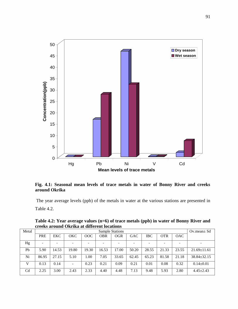
91
0
5
10
15
20
25
30
35
40
45
50C
on
ce
ntr
ati
on
(pp
b)
Hg Pb Ni V Cd
Mean levels of trace metals
Dry season
Wet season
Fig. 4.1: Seasonal mean levels of trace metals in water of Bonny River and creeks
around Okrika
The year average levels (ppb) of the metals in water at the various stations are presented in
Table 4.2.
Table 4.2: Year average values (n=6) of trace metals (ppb) in water of Bonny River and
creeks around Okrika at different locations Metal Sample Stations Ov.mean± Sd
PRE EKC OKC OOC OBR OGR GAC IBC OTR OAC
Hg - - - - - - - - - - -
Pb 5.90 14.53 19.80 19.30 16.53 17.00 50.20 28.55 21.33 23.55 21.69±11.61
Ni 86.95 27.15 5.10 1.00 7.05 33.65 62.45 65.23 81.58 21.18 38.84±32.15
V 0.13 0.14 - 0.23 0.21 0.09 0.21 0.01 0.08 0.32 0.14±0.01
Cd 2.25 3.00 2.43 2.33 4.40 4.48 7.13 9.48 5.93 2.80 4.45±2.43

92
In table 4.2, all the metals except mercury were detectable at all sample locations.
Vanadium however, was detectable only in sixteen samples representing about 26.67 % of
the total number of samples collected in the year. Nickel was particularly highest (86.95 ppb)
at this location, which is an implication for improper treatment of the refinery effluent.
However, the level was progressively lower up to OOC, and from OBR, the levels rose
sharply again up to OTR (81.58 ppb), and dropped again at OAC. The implication is that
there other sources of this metal. There are currently construction and dredging companies in
the area as indicated in section 3.1, which apart from their activities, litter the entire
waterway from OBR through OTR with broken badges and other metallic materials. Pb
levels increased also from 5.90 ppb at PRE to 50.20 ppb at GAC, and this implied that other
than the refinery, the burden of lead on the ecosystem may have been contributed by other
anthropogenic influences such as domestic wastes, the DAEWOO marine construction
company and atmospheric emissions. This may also account for the trend observed for
vanadium and cadmium.
Two-way analysis of variance showed significant (p<0.05) spatial variations in
concentrations in both dry and wet seasons.
Correlation coefficient of the pair of Ni and Pb is significant as shown in Table 4.3
below. This suggests that the two metals have a common source.
Table 4.3: Correlations matrices for the combined trace metals data of water from
Bonny River and creeks around Okrika.
Hg Pb Ni V Cd
Hg 1
Pb -1** 1
Ni 1 0.259122* 1
V . 0.118662 -0.14344 1
Cd 1** 0.227965 0.037272 -0.01078 1
. **Correlation is significant at the 0.01 level (2-tailed).
*Correlation is significant at the 0.05 level (2-tailed).
The year mean levels of major cations: Ca2+
, Mg2+
, Na+, K
+ and other physicochemical
data are presented in Tables 4.4, while seasonal levels are shown in Table 4.5a and 4.5b, and
Fig. 4.2.

93
Table 4.4: Year average (n=6) values of physico-chemical parameters (ppm, except pH, temperature, conductivity and
turbidity) in water of Bonny River and creeks around Okrika in Rivers State, Nigeria.
S/N
Parameters Sample stations Overall. mean
± SD PRE EKC OKC OOC OBR OGR GAC IBC OTR OAC
1 pH 6.87 7.01 7.64 7.56 7.65 7.71 7.48 7.78 7.60 7.26 7.45±0.31
2 Temperature 28.2 27.3 27.2 27.1 26.8 27.1 27.1 26.9 26.9 26.9 27.2±0.40
3 TDS 359.2 16,225.8 30,094.0 31,397.0 30.390.0 33,133.3 33,000.0 33,291.7 33,253.3 26,160.0 26,630 ±10,573.9
4 Salinity 180.0 8,157.3 14,808.3 15,575.0 15,075.0 15,533.0 17,033.3 16,541.7 16,575.0 13,475.0 13,295.4±5,263.8
5 Conductivity 631.3 32,025 59,038.3 60,391.7 58,983.3 62,308.3 62,665.0 63,075.0 64,080.0 48,650.0 51,184.8±20,274.9
6 Total Hardness
(Ca + Mg) 11.54 92.17 149.60 168.60 160.67 167.25 143.67 165.32 162.89 156.32S 137.80±49.74
7 Total
Alkalinity
47.5 90.8 106.4 126.8 100.9 62.1 110.9 123.8 80.9 92.5 94.3±25.4
8 BOD5 56.4 68.2 39.0 35.8 40.2 33.2 36.7 21.8 21.5 11.3 36.4±16.7
9 COD 70.0 93.7 44.1 44.4 49.2 34.9 40.3 25.5 25.5 16.7 44.4±22.8
10 DO 3.32 3.45 3.50 3.53 3.80 3.82 4.04 3.86 4.28 3.73 3.73±0.29
11 TSS 12.1 25.6 26.0 32.0 15.1 15.3 12.3 7.6 4.1 4.4 9.5±15.6
12 Turbidity 13.0 17.0 18.2 17.9 8.4 13.5 10.9 10.7 5.9 3.4 5.0±11.9
13 Silicates 0.276 2.213 2.597 2.827 2.749 2.519 2.609 2.468 2.945 3.131 2.433±0.801
14 NO3- 0.004 0.015 0.965 1.133 1.105 1.282 1.087 1.255 1.260 0.528 0.863±0.501
15 SO42-
13.9 19.4 25.1 23.6 23.9 24.7 23.0 22.8 25.1 22.7 22.4±3.4
16 PO43-
2.260 0.379 0.540 0.193 0.512 0.551 0.532 0.491 0.281 0.183 0.392±0.151
17 Ca2+
2.38 31.31 52.04 60.15 56.85 59.30 50.06 59.18 58.23 55.44 48.49±18.31
18 Mg2+
1.361 3.400 4.777 4.473 4.547 4.659 4.537 4.263 4.250 4.357 4.062±1.022
19 Na+ 9.288 12.216 12.441 12.531 12.465 12.282 12.801 12.772 12.490 11.996 12.123±1.022
20 K+ 2.872 6.869 10.700 11.082 11.411 10.936 10.175 10.301 10.540 9.918 9.480±2.463

94
Table 4.5a: Mean levels of physico-chemical parameters in water of Bonny River and creeks around Okrika in the dry season
Sample
location
Parameters
pH Temperature
(0C)
Total Dissolved Solids
(ppm)
Salinity (ppm) Conductivity (µscm-1
) Total Hardness
(Ca + Mg) (ppm)
PRE 7.25 ± 0.05 28.17 ± 0.67 466.67 ± 24.34 231.33 ± 8.39 818.33 ± 34.27 11.66 ± 2.23
EKC 7.15 ± 0.10 27.93 ± 0.64 17,036.67 ± 309.89 8,400.00 ± 229.13 33,473.33 ± 1314.58 118.06 ± 79.19
OKC 7.40 ± 0.08 27.37 ± 0.40 32,885.00 ± 248.34 16,150.00 ± 975.96 63,100.00 ± 1997.50 149.63 ± 7.76
OOC 7.50 ± 0.06 27.03 ± 0.42 35,016.67 ± 1,027.54 17,250.00 ± 409.27 66,510.00 ± 704.50 169.65 ± 2.44
OBR 7.57 ± 0.05 26.63 ± 0.23 32,968.33 ± 237.19 16,116.67 ± 857.81 63,566.67 ± 2157.16 170.89 ± 9.94
OGR 7.55 ± 0.06 27.03 ± 0.21 35,166.67 ± 611.01 17,066.67 ± 152.75 65,900.00 ± 2722.13 172.39 ± 16.91
GAC 7.71 ± 0.04 27.20 ± 0.62 34,066.67 ± 1,006.64 16,866.67 ± 208.17 65,280.00 ± 769.22 139.08 ± 31.28
IBC 7.56 ± 0.05 26.83 ± 0.31 33,066.67 ± 351.19 16,383.33 ± 381.88 64,083.33 ± 225.46 167.47 ± 10.38
OTR 7.72 ± 0.03 26.90 ± 0.36 33,266.67 ± 288.68 16,566.67 ± 305.51 65,026.67 ± 328.84 169.21 ± 12.41
OAC 2.29 ± 0.02 26,53 ± 0.25 25,816.67 ± 768.66 13,050.00 ± 1,033.20 47,566.67 ± 1075.98 155.95 ± 13.39
Range
Ov.mean±Sd (7.05-7.75)
7.47 ± 0.19
(26.50-28.60)
27.18 ± 0.62
(445-35,700)
27,975.67 ± 10,786.48
(226-17,600)
13,791.47 ± 5,333.83
(789-67,900)
53,532.50 ± 20,657.89
(9.12-191.10)
145.45 ± 54.25
Table 4.5a: Mean levels of physico-chemical parameters in water of Bonny River and creeks around Okrika in the dry season-contd
Sample
location
Total Alkalinity
(ppm)
Biological Oxygen
Demand (ppm)
Chemical Oxygen
Demand (ppm)
Dissolved
Oxygen (ppm)
Total Suspended
Solids (ppm)
Turbidity
(NTU)
SiO32-
(ppm)
PRE 33.73 ± 46.13 65.70 ± 2.85 74.13 ± 4.35 3.38 ± 0.71 13.13 ± 1.08 14.40 ± 1.64 0.11 ± 0.01
EKC 88.07 ± 18.18 76.67 ± 4.98 100.97 ± 2.29 3.23 ± 0.01 26.63 ± 3.80 18.40 ± 2.00 2.39 ± 0.53
OKC 98.00 ± 26.85 39.57 ± 0.57 49.70 ± 4.58 3.23 ± 1.00 28.33 ± 1.70 21.77 ± 1.11 2.69 ± 0.09
OOC 125.27 ± 5.83 38.00 ± 5.41 46.50 ± 1.21 3.40 ± 0.93 34.27 ± 3.91 18.70 ± 0.56 3.00 ± 0.38
OBR 98.10 ± 13.78 43.17 ± 10.90 51.60 ± 1.37 3.98 ± 0.81 20.10 ± 10.15 9.50 ± 0.98 2.87 ± 0.08
OGR 45.57 ± 56.67 32.90 ± 0.96 35.70 ± 3.84 3.74 ± 0.33 12.83 ± 2.10 15.50 ± 3.00 2.57 ± 0.60
GAC 108.90 ± 7.91 25.20 ± 5.29 25.77 ± 1.68 4.01 ± 0.65 11.63 ± 1.53 14.13 ± 0.95 2.66 ± 0.29
IBC 127.20 ± 1.39 20.40 ± 0.70 26.33 ± 2.53 4.04 ± 0.24 5.93 ± 3.20 7.50 ± 1.85 2.57 ± 0.26
OTR 80.47 ± 56.70 20.53 ± 2.01 25.40 ± 1.32 4.15 ± 0.40 3.47 ± 0.76 6.63 ± 0.80 3.14 ± 0.07
OAC 92.77 ± 15.00 11.37 ± 0.86 18.23 ± 2.06 3.78 ± 0.65 5.10 ± 1.11 3.87 ± 0.59 2.85 ± 0.13 Range
Ov.mean±Sd (6.90-132.00)
89.81 ± 39.53
(10.60-77.30)
37.35 ± 20.20
(16.10-102.80)
45.43 ± 24.92
(2.28-4.72)
3.70 ± 0.64
(2.80-38.59)
16.14 ± 10.83
(3.20-22.80)
13.04 ± 5.58
(0.01-3.25)
2.48 ± 0.87

95
Sample
location
NO3- (ppm) SO4
2-(ppm) PO4
3- (ppm) Ca
2+ (ppm) Mg
2+ (ppm) Na
+ (ppm) K
+ (ppm)
PRE 0.01 ± - 15.00 ± 3.82 0.20 ± 0.25 2.61 ± 0.51 1.98 ± 0.69 7.32 ± 0.30 2.41 ± 0.23
EKC 0.01 ± 0.00 20.27 ± 3.37 0.27 ± 0.35 37.85 ± 1.53 2.92 ± 0.13 10.51 ± 1.04 5.76 ± 2.77
OKC 0.84 ± 0.59 25.20 ± 3.40 0.19 ± 0.14 54.42 ± 0.26 2.97 ± 0.14 9.89 ± 0.61 8.49 ± 0.35
OOC 1.20 ± 0.76 23.63 ± 0.50 0.19 ± 0.02 62.74 ± 0.70 2.95 ± 0.04 10.45 ± 0.12 8.45 ± 0.35
OBR 1.17 ± 0.48 25.17 ± 1.40 0.21 ± 0.01 57.44 ± 2.10 2.93 ± 0.04 10.05 ± 0.41 8.49 ± 0.61
OGR 1.32 ± 0.14 26.01 ± 2.94 0.72 ± 0.93 61.79 ± 0.24 2.59 ± 0.45 9.62 ± 0.29 8.66 ± 0.14
GAC 1.18 ± 0.42 23.20 ± 0.52 0.87 ± 1.09 51.78 ± 6.62 2.92 ± 0.05 10.66 ± 0.73 8.23 ± 0.34
IBC 1.40 ± 0.20 24.57 ± 0.59 0.75 ± 0.83 60.66 ± 0.54 2.81 ± 0.13 10.64 ± 0.53 8.47 ± 1.48
OTR 1.48 ± 0.23 26.27 ± 2.48 0.33 ± 0.08 60.11 ± 0.54 2.77 ± 0.23 10.05 ± 0.94 8.41 ± 0.66
OAC 0.51 ± 0.02 21.97 ± 0.64 0.18 ± 0.02 54.52 ± 0.56 2.90 ± 0.09 9.64 ± 0.66 8.41 ± 0.19 Range
Ov.mean±Sd (BDL-1.740)
0.98 ± 0.55
(10.70-28.70)
23.13 ± 3.83
(0.02-2.13)
0.39 ± 0.52
(2.47-63.41)
50.39 ± 17.74
(1.52-3.12)
2.78 ± 0.37
(7.00-11.43)
9.87 ± 1.08
(2.14-9.97)
7.58 ± 2.13
Table 4.5b: Mean levels of physico-chemical parameters in water of Bonny River and creeks around Okrika in the wet season
Sample
Location
Parameters
pH Temperature
(0C)
Total Dissolved Solids
(ppm)
Salinity (ppm) Conductivity (µscm-1
) Total Hardness
(Ca + Mg) (ppm)
PRE 6.51 ± 0.09 27.13 ± 0.25 251.67 ± 16.62 128.67 ± 2.89 444.33 ± 13.58 9.90 ± 2.51
EKC 6.87 ± 0.05 26.70 ± 0.46 15,415.00 ± 410.09 7,914.00 ± 255.91 30,578.00 ± 886.55 70.30 ± 74.86
OKC 7.88 ± 0.07 27.17 ± 0.42 27,304.67 ± 870.10 13,466.67 ± 1,365.04 54,976.67 ± 297.38 149.59 ± 1.59
OOC 7.62 ± 0.67 27.07 ± 0.47 27,777.33 ± 807.43 13,900.00 ± 360.56 54,273.33 ± 933.88 174.41 ± 8.45
OBR 7.73 ± 0.06 26.87 ± 0.67 27,813.33 ± 1,036.60 14,033.33 ± 404.15 54,400.00 ± 2,137.76 177.48 ± 10.50
OGR 7.87 ± 0.15 27.23 ± 0.59 31,100.00 ± 5,200.00 14,000.00 ± 435.89 58,716.67 ± 5,833.17 166.32 ± 16.48
GAC 7.25 ± 0.28 27.37 ± 0.55 31,933.33 ± 5,063.92 17,200.00 ± 608.28 60,050.00 ± 8,463.30 155.55 ± 11.24
IBC 8.00 ± 0.17 27.10 ± 0.26 33,516.67 ± 4,417.11 16,700.00 ± 871.78 62,066.67 ± 3,807.01 174.68 ± 13.03
OTR 7.47 ± 0.42 26.80 ± 0.10 33,240.00 ± 1,566.14 16,583.33 ± 1,277.04 63,133.33 ± 3,894.01 169.28 ± 14.85
OAC 7.25 ± 0.28 27.40 ± 0.26 26,836.67 ± 1,565.58 13,900.00 ± 1,558.85 49,733.33 ± 5,115.99 163.75 ± 16.75 Range
Ov.mean±Sd (6.42-8.20)
7.44 ± 0.52
(26.10-27.90)
27.08 ± 0.43
(234-37,100)
24,702.87 ± 11,003.99
(127-17,900)
12,776.60 ± 5,032..70
(430-67,300)
48,837 ± 18,998.03
(8.42-189.60)
144.18 ± 59.26
Table 4.5a: Mean levels of physico-chemical parameters in water of Bonny River and creeks around Okrika in the dry season-contd

96
Table 4.5b: Mean levels of physico-chemical parameters in water of Bonny River and creeks around Okrika in the wet season-contd.
Sample
Location
Total Alkalinity
(ppm)
Biological Oxygen
Demand (ppm)
Chemical Oxygen
Demand (ppm)
Dissolved
Oxygen (ppm)
Total Suspended
Solids (ppm)
Turbidity
(NTU)
SiO32-
(ppm)
PRE 61.17 ± 47.37 47.10 ± 6.35 65.87 ± 4.83 3.27 ± 0.25 11.03 ± 0.68 11.50 ± 1.01 0.44 ± 0.57
EKC 93.50 ± 13.94 59.63 ± 9.50 86.40 ± 8.18 3.67 ± 0.50 24.13 ± 2.97 15.50 ± 1.47 2.04 ± 0.60
OKC 114.77 ± 30.00 38.33 ± 1.90 38.40 ± 5.07 3.76 ± 0.54 23.67 ± 2.27 14.63 ± 3.18 2.51 ± 0.12
OOC 128.30 ± 4.78 35.53 ± 0.75 42.37 ± 3.88 3.65 ± 0.99 29.67 ± 5.27 16.70 ± 1.25 2.71 ± 0.26
OBR 103.73 ± 14.46 37.13 ± 6.03 46.70 ± 2.86 3.62 ± 0.19 10.13 ± 0.40 7.37 ± 1.53 2.63 ± 0.56
OGR 78.60 ± 59.93 33.43 ± 5.17 34.07 ± 3.31 3.91 ± 0.78 17.80 ± 0.50 11.40 ± 1.10 2.46 ± 0.45
GAC 112.87 ± 9.87 48.17 ± 13.71 54.80 ± 39.03 4.06 ± 0.51 13.00 ± 1.54 7.70 ± 0.75 2.56 ± 0.39
IBC 123.57 ± 1.50 23.20 ± 6.43 24.60 ± 4.13 3.68 ± 0.47 9.23 ± 1.03 13.83 ± 0.45 2.37 ± 0.54
OTR 138.47 ± 45.60 22.53 ± 1.68 25.70 ± 2.52 4.40 ± 0.49 4.67 ± 3.43 5.20 ± 0.50 2.75 ± 0.13
OAC 92.27 ± 11.35 11.20 ± 1.65 15.07 ± 1.27 3.69 ± 0.77 3.70 ± 0.69 2.90 ± 0.62 3.41 ± 0.65 Range
Ov.mean±Sd (6.50-190.00)
104.72 ± 34.08
(10.10-69.30)
35.42 ± 14.72
(10.40-95.70)
43.39 ± 23.21
(2.53-4.75)
3.77 ± 0.57
(2.30-33.10)
14.70 ± 8.69
(2.20-18.30)
10.67 ± 4.66
(0.11-3.97)
2.39 ± 0.83
Table 4.5b: Mean levels of physico-chemical parameters in water of Bonny River and creeks around Okrika in the wet season-contd.
Sample
location
NO3- (ppm) SO4
2-(ppm) PO4
3- (ppm) Ca
2+ (ppm) Mg
2+ (ppm) Na
+ (ppm) K
+ (ppm)
PRE 0.01 ± 0.00 12.87 ± 3.33 0.32 ± 0.25 2.16 ± 0.70 0.75 ± 0.03 11.25 ± 4.54 3.34 ± 1.60
EKC 0.02 ± 0.01 18.47 ± 3.14 0.48 ± 0.38 24.78 ± 1.46 3.88 ± 1.88 13.92 ± 6.53 6.31 ± 0.24
OKC 1.09 ± 0.58 25.00 ± 0.89 0.89 ± 1.16 49.66 ± 13.17 6.58 ± 3.25 14.99 ± 4.71 12.91 ± 4.26
OOC 1.07 ± 0.17 23.60 ± 2.74 0.20 ± 0.01 57.56 ± 3.61 6.00 ± 2.70 14.61 ± 5.26 13.72 ± 4.40
OBR 1.04 ± 015 22.67 ± 0.40 0.15 ± 0.05 56.26 ± 3.68 6.16 ± 2.83 14.88 ± 5.05 13.82 ± 3.40
OGR 1.24 ± 0.24 23.30 ± 1.64 0.38 ± 0.31 56.81 ± 5.43 6.72 ± 3.14 15.94 ±5.13 12.74 ± 5.80
GAC 1.33 ± 0.61 22.87 ± 1.16 0.19 ± 0.05 48.33 ± 14.17 6.15 ± 3.73 14.94 ± 5.08 12.13 ± 5.34
IBC 1.11 ± 0.34 20.93 ± 0.85 0.38 ± 0.29 57.66 ± 2.65 5.72 ± 3.56 14.79 ± 5.02 12.79 ± 5.88
OTR 1.04 ± 0.37 24.00 ± 1.01 0.23 ± 0.05 56.34 ± 3.82 5.37 ± 3.37 14.93 ± 5.96 12.66 ± 5.23
OAC 0.55 ± 0.20 23.47 ± 4.02 0.18 ± 0.05 56.36 ± 4.74 5.82 ± 3.08 14.36 ± 5.44 11.42 ± 4.63 Range
Ov.mean±Sd (BDL-1.96)
0.88 ± 0.53
(10.70-27.70)
21.7 ± 3.95
(0.04-2.23)
0.34 ± 0.41
(1.57-60.74)
46.59 ± 18.79
(0.72-8.88)
5.31 ± 2.99
(6.01-18.93)
14.36 ± 4.54
(1.50-16.48)
11.18 ± 4.99

97
Mean pH in the dry season was 7.47 ± 0.19. In the wet season, it was 6.42 - 8.20 and the
overall mean was 744 ± 0.52. Salt intrusion at all stations was evident with very high levels
of salinity, producing a brackish condition all over. Mean temperature was 27.18 ± 0.62 in
the dry season, while in the wet season, it was 27.08 ± 0.43. There was no significant change
in temperature (p>0.05). Total dissolved solids (TDS) ranged from 445 - 35, 700 ppm in the
dry season with an overall mean level of 27,797.67 ± 10,786.48. In the wet season, it was
from 234 -37,100 ppm with a mean level of 24,702.87 ± 11,003.99. Salinity levels ranged
from 226 - 27,600 ppm with a mean level of 13,791.47 ± 5,333.83. In the wet season, the
range was 127 - 17,900 ppm with a mean level of 12,776.60 ± 5,032.70. Conductivity levels
in the dry season ranged from 789-67,900 µscm-1
with a mean level of
53,532.50 ± 29,657.89. In the wet season the ranged was from 430 – 67,300 µscm-1
with a
mean level of 48,837 ± 18,998.03. Seasonal change was not significant (p>0.05).
Levels of hardness (Ca + Mg) ranged from 9.12 – 191.29 ppm with a mean level of
145.45 ± 54.25 in the dry season. In the wet season, the range was 8.42 – 189.29 ppm with a
mean level of 144.18 ± 59.26. Seasonal variation was insignificant (p>0.05) on the
`combined data of Ca and Mg. However, t-test on each of Ca and Mg data indicated Mg
seasonally variable (p<0.05). Levels of total alkalinity in the dry season ranged from
6.90-132 ppm with a mean of 89.81 ± 39.53. In the wet season, it was from 6.50-190 ppm
with a mean of 104.72 ± 34.08. Seasonal difference was significant (p<0.05). Levels of total
suspended solids (TSS) ranged in the dry season from 2.90-38.59 ppm with a mean of
16.14 ± 10.83, whereas in the wet season, the range was 2.30-33.10 ppm with a mean of
14.70 ± 8.69. Seasonal difference was insignificant (p>0.05). Turbidity levels ranged from
3.20 – 22.80 NTU in the dry season with a mean level of 13.04 ± 5.84. In the wet season, it
ranged from 2.20-18.30 NTU with a mean level of 10.67 ± 4.66. Seasonal variation was not
significant (P>0.05).
Biological oxygen demand (BOD) levels ranged from 10.60 - 77.30 ppm with a mean of
37.35 ± 20.20 in the dry season. In the wet season, the range was from 10.10 -69.30 ppm
with a mean of 35.42 ± 14.72. Chemical oxygen demand (COD) ranged from 16.10 - 102.80
ppm with a mean level of 45.43 ± 24.92 in the dry season. In the wet season, the range was
from 10.40 - 95.70 ppm with a mean of 43.39 ± 23.21. Dissolved oxygen (DO) levels ranged
98
in the dry season from 2.28 - 4.72 ppm with a mean of 3.79 ± 0.64. In the wet season, the
range was from 2.53-4.75 ppm with a mean of 3.77 ± 0.57.
Levels of silicates in the dry season ranged from 0.01 – 3.25 ppm with a mean of
2.48 ± 0.87, while in the wet season, the range was from 0.11 – 3.97 ppm with a mean of
2.39 ± 0.83. Levels of nitrate in the dry season ranged from below detection limits (BDL)
to1.74 ppm with a mean of 0.98 ± 0.55. In the wet also, it ranged from BDL to1.96 ppm with
a mean of 0.88 ± 0.53. Sulphate levels in the dry season ranged from 10.70 – 28.70 ppm with
a mean of 23.13 ± 3.83. In the wet season, the range was from 10.70 – 27.70 ppm with a
mean of 21.70 ± 3.95. Phosphate levels in the dry season ranged from 0.02 – 2.13 ppm with a
mean of 0.39 ± 0.52. In the wet season, the range was from 0.04 – 2.23 ppm with a mean of
0.34 ± 0.41. Seasonal levels of these nutrient were however comparable (p>0.05).
Sodium levels in the dry season ranged from 7.00 – 11.43 ppm with a mean of
9.87 ± 1.08. In the wet season, the range was from 6.01 – 18.93 ppm with a mean of
14.36 ± 4.54. Seasonal levels differed significantly (p<0.05) with higher levels in the wet
season. Potassium levels in the dry season ranged from 2.14 – 9.97 ppm with a mean of
7.58 ± 2.13. In the wet season, the range was from 1.50 -16.48 ppm with a mean of
11.18 ± 4.99. Seasonal variation was significant (p<0.05).

99
Fig. 4.2: Mean seasonal values of physicochemical parameters in water of Bonny River and creeks around Okrika.
7.425
7.43
7.435
7.44
7.445
7.45
7.455
7.46
7.465
7.47p
H v
alu
es
DRY WET
Seasons of the year
27.02
27.04
27.06
27.08
27.1
27.12
27.14
27.16
27.18
Tem
p. (0
C)
DRY WET
Seasons of the year
23,000.00
24,000.00
25,000.00
26,000.00
27,000.00
28,000.00
TD
S (
pp
m)
DRY DRY
Seasons of the year
12,200.00
12,400.00
12,600.00
12,800.00
13,000.00
13,200.00
13,400.00
13,600.00
13,800.00
Salin
ity (
pp
m)
DRY WET
Seasons of the year
46,000.00
47,000.00
48,000.00
49,000.00
50,000.00
51,000.00
52,000.00
53,000.00
54,000.00
Co
nd
. (u
cm
s-1
)
DRY WET
Seasons of the year
143.50
144.00
144.50
145.00
145.50
To
tal H
ard
nes
s
(Ca+
Mg
)-p
pm
DRY WET
Seasons of the year
80.00
85.00
90.00
95.00
100.00
105.00
To
tal A
lkalin
ity (
pp
m)
DRY WET
Seasons of the year
34.00
34.50
35.00
35.50
36.00
36.50
37.00
37.50
BO
D5 (
pp
m)
DRY WET
Seasons of the year
42.00
42.50
43.00
43.50
44.00
44.50
45.00
45.50
CO
D (
pp
m)
DRY WET
Seasons of the year

100
Fig. 4.2: Mean seasonal values of physicochemical parameters in water of Bonny River and creeks around Okrika- contd.
3.66
3.68
3.70
3.72
3.74
3.76
3.78
DO
(p
pm
)
DRY WET
Seasons of the year
13.50
14.00
14.50
15.00
15.50
16.00
16.50
TS
S (
pp
m)
DRY WET
Seasons of the year
0.00
2.00
4.00
6.00
8.00
10.00
12.00
14.00
Tu
rbid
ity (
NT
U)
DRY WET
Seasons of the year
2.34
2.36
2.38
2.40
2.42
2.44
2.46
2.48
Silic
ate
s (
pp
m)
DRY WET
Seasons of the year
0.82
0.84
0.86
0.88
0.90
0.92
0.94
0.96
0.98
Nit
rate
(p
pm
)DRY DRY
Seasons of the year
21.00
21.50
22.00
22.50
23.00
23.50
Su
lph
ate
(p
pm
)
DRY WET
Seasons of the year
0.31
0.32
0.33
0.34
0.35
0.36
0.37
0.38
0.39
Ph
osp
hate
(p
pm
)
DRY WET
Seasons ot the year
44.00
45.00
46.00
47.00
48.00
49.00
50.00
51.00
Calc
ium
(p
pm
)
DRY WET
Seasons of the year
0.00
1.00
2.00
3.00
4.00
5.00
6.00
Mag
nesiu
m (
pp
m)
DRY WET
Seasons of the year

101
Fig. 4.2: Mean seasonal values of physicochemical parameters in water of Bonny River
and creeks around Okrika- contd.
Tables 4.6a and 4.6b show the matrices of correlation coefficients between trace metals and
physicochemical parameters measured in surface water of Bonny River and creeks around
Okrika. Some significant correlation coefficients /r/ were seasonal. In the dry season,
significant correlation coefficients were those of Pb/temp; Pb/BOD; Pb/PO43-
; V/PO43-
;
Cd/PO43-
(p<0.01, 0.01; 0.05; 0.01; 0.01). Significant metal/metal correlation coefficients
was also found for Ni/Pb (p<0.05) in this season. In the wet season, the significant
correlations were Pb/Mg2+
; Pb/Na+; Pb/K
+; Ni/Mg
2+; Ni/Na
+; Cd/Na
+ and Cd/TDS (P<0.05;
0.05; 0.01; 0.01; 0.01; 0.01; 0.01; 0.01). These differing associations in the two seasons may
be due to seasonal diagenetic changes. However, a combination of both seasons also revealed
many pairs (Appendix M).
0.00
2.00
4.00
6.00
8.00
10.00
12.00
14.00
16.00
So
diu
m (
pp
m)
DRY WET
Seasons of the year
0.00
2.00
4.00
6.00
8.00
10.00
12.00
Po
tass
ium
(p
pm
)
DRY WET
Seasons of the year

102
Table 4.6a: Correlation matrices: Trace metals versus
physicochemical parameters in the dry season Hg Pb Ni V Cd
pH - 0.099 0.114 0.544 0.097
Temperature - -0.411* 0.236 -0.088 -0.219
TDS - 0.297 -0.228 0.255 0.112
Salinity - 0.282 -0.231 0.232 0.123
Conductivity - 0.243 -0.212 0.227 0.130
TH - 0.353 -0.261 0.314 0.119
TA - 0.419 -0.241 -0.048 0.153
BOD5 - -0.298* -0.018 -0.453 -0.153
COD - -0.270 -0.062 -0.538 -0.132
DO - 0.330 0.160 0.655 0.142
TSS - -0.117 -0.348 -0.627 -0.223
Turbidity - -0.013 -0.259 -0.333 -0.223
SiO32-
- 0.124 -0.250 0.274 0.102
NO3-
- 0.364 0.007 0.271 0.238
SO42-
- 0.020 -0.044 0.257 0.127
PO43-
- 0.621** -0.238 0.819* 0.409*
Ca2+
- 0.231 -0.183 -0.012 0.136
Mg2+
- -0.137 -0.251 0.002 -0.022
Na+ - 0.044 0.021 0.214 0.177
K+ - 0.174 -0.237 0.150 -0.028
* p<0.05 ● TH- total hardness
** p<0.01 ● TA- total alkalinity
Table 4.6b: Correlation matrices: Trace metals versus
physicochemical parameters in the wet season Hg Pb Ni V Cd
pH - -0.087 -0.072 0.450 0.336
Temperature - 0.090 0.187 0.352 -0.035
TDS - 0.250 -0.070 0.319 0.396*
Salinity - 0.313 -0.139 0.347 0.307
Conductivity - 0.200 -0.083 0.285 0.323
TH - 0.123 -0.279 0.305 0.158
TA - -0.073 -0.258 -0.119 0.201
BOD5 - 0.168 0.031 -0.592 -0.143
COD - -0.065 0.140 -0.619 -0.301
DO - 0.126 -0.004 -0.275 -0.098
TSS - -0.090 -0.176 -0.411 -0.222
Turbidity - -0.111 -0.150 -0.435 -0.174
SiO32-
- 0.141 -0.175 0.513 0.257
NO3-
- 0.240 0.159 -0.049 0.052
SO42-
- 0.080 -0.120 0.459 0.095
PO43-
- -0.137 -0.121 -0.231 -0.110
Ca2+
- 0.253 -0.295 0.411 0.121
Mg2+
- 0.503** -0.469** 0.306 -0.301
Na+ - 0.500** -0.521** 0.528 -0.425
K+ - 0.411* -0.486* 0.412 -0.187

103
The significant correlations between PO43-
and Pb, V and Cd in the dry season suggest that
these metals are present in their phosphates probably as particulates. The association of these
metals with phosphate in water, may to a large extent, be due to refinery effluent as the year
average concentration of phosphate in the effluent was highest. In the wet season, the
correlations between major metal cations and the trace metals, Pb and Ni are however not easily
explicable, but that of Cd and TDS is an indication that most of the cadmium is in solution. The
negatively significant correlations between the trace metals and physicochemical parameters in
both seasons may suggest inhibitive tendencies of these water parameters towards mobilization
of these metals to the water column.
4.2: Results of sediment analysis
Year average concentrations of trace metals in the sediment are presented in Table 4.7.
Table 4.7: Year average (n=6) values (ppm, dry wt.) of parameters in sediment of Bonny
River and creeks around Okrika
S/N
Parameters
Sample stations
Ov.mean±SD PRDC EKC OKC OOC OBR OGR GAC IBC OTR OAC
1 Hg 0.068 0.018 0.011 0.036 0.021 0.015 0.020 0.034 0.032 0.023 0.273±0.016
2 Pb 4.210 2.167 33.822 19.058 37.439 26.848 11.693 27.808 29.034 40.104 23.218±13.427
3 Ni 51.871 46.467 62.413 86.579 44.029 46.746 31.513 81.004 58.188 63.125 57.194±16.929
4 V* 0.017 0.07 0.023 0.013 0.146 0.069 0.125 0.029 0.023 0.083 0.060
5 Cd* 0.044 0.438 0.195 0.062 1.005 0.091 0.018 0.023 0.254 0.173 0.130
6 TOC (%) 0.484 0.753 1.430 1.005 1.404 1.199 0.971 0.802 1.535 1.767 1.135±0.401
7 TOM (%) 0.834 1.234 2.467 1.735 2.421 2.070 1.675 1.385 2.650 3.073 1.99±0.703
PRDC – Port Harcourt Refinery discharge channel
* Values only detectable
The estimated values of trace metals (ppm, dry weight) and organic matter (%) of sediment
in the year are as follows: Hg (0.273 ± 0.016); Pb (23.218 ± 13.427); Ni (57.194 ± 16.929); TOC
(1.135 ± 0.401) and TOM (1.990 ± 0.703). V and Cd only showed detectable values representing
21.67 % and 31.67 % respectively. The levels of Ni and Pb are appreciable both in the effluent
discharge channel sediment and those of other sampling stations. This suggests that these metals
may have had their way into the sediment by activities other than those of the refinery.
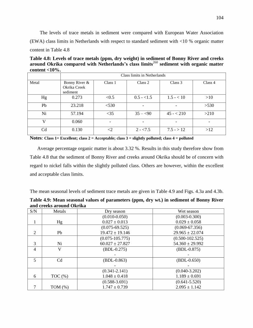
104
The levels of trace metals in sediment were compared with European Water Association
(EWA) class limits in Netherlands with respect to standard sediment with <10 % organic matter
content in Table 4.8
Table 4.8: Levels of trace metals (ppm, dry weight) in sediment of Bonny River and creeks
around Okrika compared with Netherlands’s class limits260
sediment with organic matter
content <10%. Class limits in Netherlands
Metal Bonny River &
Okrika Creek
sediment
Class 1 Class 2 Class 3 Class 4
Hg 0.273 <0.5 0.5 - <1.5 1.5 - < 10 >10
Pb 23.218 <530 - - >530
Ni 57.194 <35 35 – <90 45 - < 210 >210
V 0.060 - - - -
Cd 0.130 <2 2 - <7.5 7.5 - > 12 >12
Notes: Class 1= Excellent; class 2 = Acceptable; class 3 = slightly polluted; class 4 = polluted
Average percentage organic matter is about 3.32 %. Results in this study therefore show from
Table 4.8 that the sediment of Bonny River and creeks around Okrika should be of concern with
regard to nickel falls within the slightly polluted class. Others are however, within the excellent
and acceptable class limits.
The mean seasonal levels of sediment trace metals are given in Table 4.9 and Figs. 4.3a and 4.3b.
Table 4.9: Mean seasonal values of parameters (ppm, dry wt.) in sediment of Bonny River
and creeks around Okrika S/N Metals Dry season Wet season
1
Hg
(0.010-0.050)
0.027 ± 0.013
(0.003-0.300)
0.029 ± 0.058
2
Pb
(0.075-69.525)
19.472 ± 19.146
(0.069-67.356)
29.965 ± 22.074
3
Ni
(0.075-105.775)
60.027 ± 27.827
(0.500-102.525)
54.360 ± 29.992
4 V (BDL-0.275)
-
(BDL-0.875)
-
5 Cd (BDL-0.863)
-
(BDL-0.650)
-
6
TOC (%)
(0.341-2.141)
1.048 ± 0.418
(0.040-3.202)
1.189 ± 0.691
7
TOM (%)
(0.588-3.691)
1.747 ± 0.739
(0.641-5.520)
2.095 ± 1.142

105
0
10
20
30
40
50
60
70co
nc.
(pp
m)
Hg Pb Ni V Cd
Trace metals
Dry season
Wet season
Fig. 4.3a: Mean seasonal levels of trace metals in sediment of Bonny River and creeks
around Okrika
0
0.5
1
1.5
2
2.5
Le
ve
ls(%
)
TOC TOM
Organic matter
Dry season
Wet season
Fig. 4.3b: Mean seasonal levels of organic matter in sediment of Bonny River and creeks
around Okrika

106
The seasonal levels were only significant (p<0.05) for Pb and TOM.
Matrices of correlation coefficient /r/ given in Tables 4a and 4b showed that there were both
seasonal and spatial variations. The pairs that were significant in dry season were V/Pb and
Cd/Pb (p<0.05). Pairs of V/Ni, Pb/TOC, Pb/TOM and TOC/TOM (P<0.01) were significant in
both dry and wet season.
Table 4.10a: Correlation matrices of trace metals and organic matter in sediment of Bonny
River and creeks around Okrika for dry season Hg Pb NI V Cd TOC TOM
Hg 1
Pb -0.16787 1
NI 0.119935 -0.20297 1
V -0.13595 0.294878* -0.35906** 1
Cd -0.10131 0.258518 -0.21362* -0.07992 1
TOC -0.1692 0.504208 -0.07938** 0.027149 0.12231 1
TOM -0.17004 0.472626 0.001751** 0.030523 -0.11363 0.936481** 1
* correlation is significant at the 0.05 level (2-tailed)
** correlation is significant at the 0.01 level (2-tailed)
Table 4.10b: Correlation matrices of trace metals and organic matter in sediment of Bonny
River and creeks around Okrika for wet season Hg Pb Ni V Cd TOC TOM
Hg 1
Pb -0.17681 1
Ni 0.09488 -0.19358 1
V -0.14749 0.285027 -0.48197** 1 .
Cd a. a. a. a. a. . .
TOC -0.22792 0.569866** -0.10655 0.054137 .a 1
TOM -0.25991 0.581137** -0.04885 0.036772 .a 0.961787** 1
** correlation is significant at the 0.01 level (2-tailed)
a cannot be computed because at least one of the variables is constant
The correlation between TOC, TOM and Pb in the wet season suggests that an important
source of lead in the water is organic loading by runoff water.
4.3: Results of refinery effluent/wastewater analysis
The mean levels of trace metals (ppb) in effluent/wastewater are compared with
effluent/wastewater limitation guidelines for petroleum refineries and other categories of
industrial wastes in Nigeria and presented in Table 4.11.

107
Table 4.11: Trace metal levels (ppb) in refinery effluent/wastewater compared with effluent
(wastewater) limitation guidelines in Nigeria179
. Metal Mean levels of trace metals in refinery
effluent
Effluent/wastewater limitation guideline for
petroleum refinery and other categories of industries
in Nigeria
Hg BDL 50
Pb 5.90 ± 6.04 <50
Ni 86.95 ± 110.39 <1000
V 0.13 ± 0.21 -
Cd 2.29 ± 2.37 10
Mercury was not detectable, but the detectable levels of lead, nickel, vanadium and
cadmium were quite below limits set for petroleum and allied wastes in Nigeria. However, the
presence of Pb, V and Ni in the effluent and their absence as recorded in Table 2.1, is an
indication that effluent quality, quantity and composition may change with changing logistics
during the routine shifts run by the refinery1.
4.4: Results of shellfish and fish analysis
The muscle tissues of shellfish and fish alone were used for the determination of trace metal
levels in them. The mean levels are presented in Table 4.12 and Fig. 4.4
Table 4.12: Mean levels (ppm) of trace metals in shellfish and fish (dry weight) of Bonny
River and creeks around Okrika
Metals Shellfish Fish
P. aurita G. rhizophorea P. koelreuteri M. cephalus S. marderensis T. guineensis
Hg (0.006-0.040)
0.016±0.012
(0.002-0.090)
0.018±0.026
(0.003-0.050)
0.014±0.019
(0.003-0.030)
0.011±0.010
(0.003-0.040)
0.008±0.011
(0.003-0.080)
0.026±0.032
Pb (0.030-2.850)
1.241±0.012
(0.028-2.450)
1.193±0.697
(0.050±0.658)
0.212±0.228
(0.263-4-675)
1.904±1.944
(0.118-2.178)
0.815±0.932
(0.050-2.888)
0.627±1.110
Ni (0.093-38.425)
11.058±12.509
(0.115-80.275)
19.923±27.036
(0.153-41.850)
11.131±16.817
(0.153-37.528)
16.591±18.132
(0.093-44.725)
8.039±18.007
(0.038-0.920)
0.567±0.658
V BDL BDL BDL BDL BDL BDL
Cd (0.050-1.180)
0.391±0.393
(0.028-0.180)
0.094±0.041
(0.050-0.525)
0.093±0.090
(BDL-1.650)
-
(BDL-1.075)
-
(BDL-1.375)
-
BDL: below detection level
Vanadium was below detection level in both fish types.

108
0
2
4
6
8
10
12
14
16
18
20C
on
c.
(pp
m)
P. aurita G. rhizophorea P. koelreuteri M. cephalus S. marderensis T. guineensis
Shellfish and fish
Hg
Pb
Ni
V
Cd
Fig. 4.4: Mean levels of trace metals in shellfish and fish of Bonny River and creeks around
Okrika
Two-way analysis of variance showed no significant difference (p>0.05) with respect to the
Pb, Ni and Cd in P. aurita. However, the combined data of their means revealed significant
variations (p<0.05) in the metal uptake. In P. aurita, Hg, Ni and Cd concentrations were lower at
Ekerekana creek (EKC) than in those obtained from Okpoka Toru River (OTR). In G.
rhizophorea, Hg and Ni were lower at EKC, while Pb recorded lower value at OTR. Ni generally
gave the highest accumulation in both shellfish. The order of metal accumulation in shellfish was
Ni> Pb> Cd> Hg
The levels of metal accumulation in fish followed the same order as in shellfish: Ni> Pb>
Cd> Hg. Vanadium was not detectable in any sample while cadmium was detectable in some
samples of M. cephalus, S. marderensis, and T. guineensis representing about 55.56 % of total
number of samples analysed from these fish samples.
Bioaccumulation factors (ratio of metal level in tissue to metal levels in water) are presented
in Table 4.13. The data showed that in the shellfish, bioaccumulation factor (BF) was higher for
Pb and Ni in P. aurita and Hg and Cd in G. rhizophorea. The factor was however generally
higher in G. rhizophorea than P. aurita with respect to Cd. Bioaccumulation factor for fish
samples were in the following order: Hg: T. guineensis >P. koelreuteri >M. cephalus > S.
marderensis; Pb: M. cephalus > S. marderensis > T. guineensis > P. koelreuteri; Ni: M. cephalus
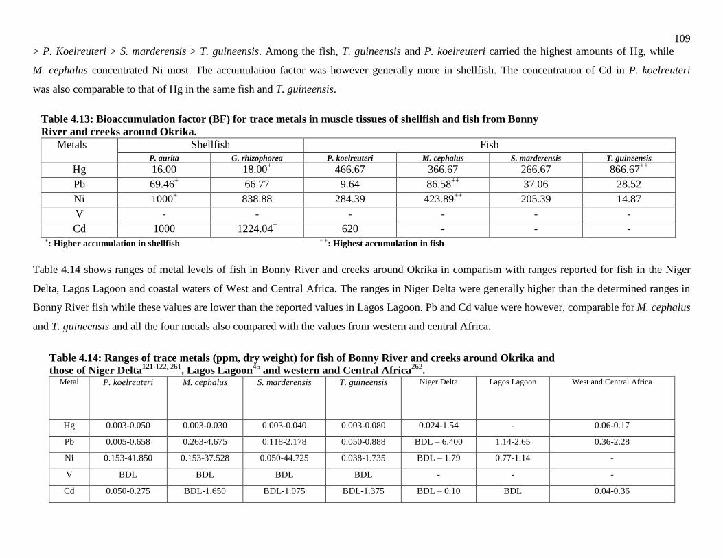
109
> P. Koelreuteri > S. marderensis > T. guineensis. Among the fish, T. guineensis and P. koelreuteri carried the highest amounts of Hg, while
M. cephalus concentrated Ni most. The accumulation factor was however generally more in shellfish. The concentration of Cd in P. koelreuteri
was also comparable to that of Hg in the same fish and T. guineensis.
Table 4.13: Bioaccumulation factor (BF) for trace metals in muscle tissues of shellfish and fish from Bonny
River and creeks around Okrika.
Metals Shellfish Fish
P. aurita G. rhizophorea P. koelreuteri M. cephalus S. marderensis T. guineensis
Hg 16.00 18.00+ 466.67 366.67 266.67 866.67
++
Pb 69.46+ 66.77 9.64 86.58
++ 37.06 28.52
Ni 1000+ 838.88 284.39 423.89
++ 205.39 14.87
V - - - - - -
Cd 1000 1224.04+ 620 - - -
+: Higher accumulation in shellfish
+ +: Highest accumulation in fish
Table 4.14 shows ranges of metal levels of fish in Bonny River and creeks around Okrika in comparism with ranges reported for fish in the Niger
Delta, Lagos Lagoon and coastal waters of West and Central Africa. The ranges in Niger Delta were generally higher than the determined ranges in
Bonny River fish while these values are lower than the reported values in Lagos Lagoon. Pb and Cd value were however, comparable for M. cephalus
and T. guineensis and all the four metals also compared with the values from western and central Africa.
Table 4.14: Ranges of trace metals (ppm, dry weight) for fish of Bonny River and creeks around Okrika and
those of Niger Delta121-122, 261
, Lagos Lagoon45
and western and Central Africa262
. Metal P. koelreuteri M. cephalus S. marderensis T. guineensis Niger Delta
Lagos Lagoon
West and Central Africa
Hg 0.003-0.050 0.003-0.030 0.003-0.040 0.003-0.080 0.024-1.54 - 0.06-0.17
Pb 0.005-0.658 0.263-4.675 0.118-2.178 0.050-0.888 BDL – 6.400 1.14-2.65 0.36-2.28
Ni 0.153-41.850 0.153-37.528 0.050-44.725 0.038-1.735 BDL – 1.79 0.77-1.14 -
V BDL BDL BDL BDL - - -
Cd 0.050-0.275 BDL-1.650 BDL-1.075 BDL-1.375 BDL – 0.10 BDL 0.04-0.36

110
Table 4.15 shows legal limits of two of the metals (Pb and Cd) in Australia263
, South East Asia264
, and New Zealand264
and are compared with
mean levels in Bonny River and creeks around Okrika fish and shellfish muscle tissues.
Table 4.15: Limits of some trace metals in shellfish and fish acceptable in some countries compared with mean levels of metals
in Bonny River and creeks around Okrika (ppm, dry weight). Bonny River and Creeks around Okrika Legal limits
Fish Shellfish Australia
South-East Asia
New Zealand
Metal P.
koelreuteri
M. cephalus S. marderensis T. guineensis P.aurita G. rhizophorea Shellfish Fish Shellfish Fish Shell fish Fish
Hg 0.014 0.011 0.008 0.026 0.006 0.002 - - - - - -
Pb 0.213 1.094 0.815 0.627 0.030 0.028 5.0 1.5 - 0.02 - -
Ni 11.131 16.591 8.039 0.567 0.093 0.115 - - - - - -
V BDL BDL BDL BDL BDL BDL - - - - -
Cd 0.093 - - - 0.050 0.028 2.0 0.2 - <0.002 - 1.0
Lead levels in fish were slightly higher than the legal limits in South East Asia, but lower than that in Australia except for M. cephalus. Lead levels
in P. aurita and G .rhizophorea were also lower than that in Australia. Cd on the other hand also recorded slightly higher levels in fish than that in
South East Asia, but lower than that of Australia and New Zealand. The levels in P. aurita and G. rhizophorea were equally lower in Australia.
4.5: Discussion
Sampling in dry and wet season was to investigate seasonal variabilities of trace metal levels and assess the contribution of runoff water
toward trace metal enrichment; also to investigate seasonal changes in levels of some water chemical parameters and how these changes affect the
levels of trace metals in water. For instance, correlation matrices of trace metals and physicochemical parameters in water (Tables 4.6a and 4.6b)
showed that in the dry season, most of the metals existed probably as particulate phosphates mainly from the refinery effluents which showed the
highest concentration of phosphate (Table 4.4), whereas in the wet season they seemed to have disappeared due probably to inhibitive tendencies of
the major cations.
In order to avoid contaminating the field samples, sampling materials and containers were cleaned using appropriate reagents, and for
sediment, they were taken from the centre of the grab. Deep-freezing was used as the method of sample preservation since it allows only the least
111
changes in the sample during storage. It also makes it unnecessary to add chemicals which could
contaminate the samples. The discharge of effluents from the Port Harcourt Refining Company
(which the study considers a point source) into the studied area, is a continuous process. Effluent
components and characteristics in terms of quality and quantity are known to differ significantly
not only due to seasonal or weather changes1, but also changing logistics. For this reason, a truly
representative portion (sampling) was guided by collection of the samples within periods that
presumably cover at least two of the operational three shifts run by the company during which
changes in the composition of the effluents may occur. In addition, samples were collected
during mid-ebb periods of low tide to ensure that the influences that were being sought were
from the point source, and not necessarily from the receiving water body.
The method of digesting the sediment samples analyzed was convenient and fast. Small
amounts of reagent were used, and carried out at low temperature (60 oC). The low digestion
temperature greatly reduced the risk of explosion and the requirements for close attention during
digestion. The use of APDC/MIBK chelation/extraction system was to (i) minimize the
interference of major cations that scatter flame, and (ii) to concentrate the metals and increase
sensitivity of the technique. For any technique to be of value, it is essential that standards closely
resemble the samples with respect to the concentration range of analyte(s) and the matrix of the
sample. Thus, standard solutions were made to undergo the same procedure as the samples. Such
technique tends to minimize matrix differences between samples and standards and the errors in
determination that could arise from such effect. It also compensates for lapses in the efficiency of
the analytical procedure.
The most frequently used solvent for ammonium pyrrolidine dithiocarbamate (APDC) is
methyl isobutyl ketone (MIBK). It provides a stable flame in atomic absorption flame
spectrophotometer (AAFS) and its physical properties such as viscosity, surface tension, boiling
point and mutual solubility in an aqueous solution are favourable. It gives a low background in
the flame215, 239
.
4.5.1: Trace metals in water and sediment
Wastes entering aquatic systems go into the ecosystem. The response of an aquatic system
to waste input is a function of the characteristics of the ecosystem, the nature, quality and
quantity of wastes265
. The capacity of any particular aquatic system to transform wastes without

112
damage to the ecosystem (self-purification) is a function of the complexity of such
environmental factors as the water flow velocity, volume of water, bottom contour, rate of water
exchange, currents, depth, light penetration and temperature, as well as re-aeration capacity and
chemical and biological interaction within the system265
. Most flowing systems have greater re-
aeration capacity than standing waters, and flowing system are “open systems” with continual
renewal of water; whereas standing systems such as lagoons are “closed systems”, and act as
“traps” for pollutants. Thus, the system studied which could be considered ‘open’, has high
capacity for self-purification, hence organic matter is less than 10 % and trace metals content in
the sediment fall within excellent and acceptable levels (Table 4.8) and considered non polluting.
Temperature and dissolved oxygen play vital roles in the rate of chemical reaction and the
nature of biological activities, and thus governing the assimilative capacity of aquatic systems.
Year average temperature in the present study was about 27 oC, while, the upper limit for
survival fish266
is 36 oC. The low temperature could be attributed to over-hanging macrophytes
which prevent sunlight on the water266
. Average DO was 3.7 mgl-1
. This condition does not
suggest pollution considering the fact that in worst conditions such as in warm water
conditions130
, DO concentrations range from 4-1 mgl-1
. Fish needs at least 2 mgl-1
DO
concentration to survive170
. In waters where there is little mixing and in organically enriched
systems, depletion of dissolved oxygen typically occurs in the bottom layer because there is little
or no photosynthetic activities or little or no mixing with oxygen – rich surface layer. This leads
to reducing conditions which can remobilize trace metals234, 265
. However, average value of 3.7
mgl-1
for DO in this shows much depletion may have occurred caused by oxygen consuming
chemicals with BOD and COD levels being 35-37 ppm and 43-45 ppm respectively.
The levels of BOD5, and COD are quite considerable and could be ascribed to organic
contamination entering the system from municipal and industrial effluents due to urban life and
many industrial establishments. These organic materials eventually get broken down by bacteria,
which require oxygen for the decomposition process, leading to depletion of DO, hence the low
DO content of the water. This conforms to other reports that a low DO indicates a high COD and
BOD5 values267
.
Water hardness, alkalinity, pH (associated with buffering capacity) and nutrients such as
nitrates, carbonates, and phosphates, are some of the other important chemical characteristics
governing the nature and quantity of wastes in the different phases of a natural aquatic system265
.

113
The chemical parameters, because of synergistic and antagonist interactions together in part,
determine the general physiochemical condition prevailing in the water system, and in this way,
play significant roles in the distribution of pollutants such as the trace metals between the water
column, sediment and organisms.
The remarkable spatial and seasonal variations in the metal-metal correlation matrices could
only be ascribed to substantial anthropogenic input of metals into the water from direct waste
discharge and many diffuse sources. Significant correlations /r/ between sediment metal levels
was obtained in the dry season when the system was less disturbed. In the dry season (Table
4.10a), the negative correlation (p<0.05) of Ni against Cd and V seems to suggest that Ni has a
different diagenesis from those of Cd and V. Also in Table 4.6b, while Pb showed positive
correlation (p<0.05) with the major cations, Ni showed negative correlation (p<0.05) with the
same ions, implying differences in diagenesis. In the wet season (Table 4.10b), there is indication
that Pb is more associated with organic matter, due most likely from land-derived wastes brought
in by runoff water.
The absence of significant seasonal differences (p>0.05) in the concentrations of trace
metals except Pb and TOM, may be explained as resulting from high flushing and dilution rates
during the rains, in addition to the associated velocity of the system or “solution effect”
consequent upon a process whereby ions bound in previous semi-dry land by decaying
macrophytes get dissolved as water levels increased with inundation of fringing swamps and
riparian zones266, 268
.On the other hand, in the dry season, the inflow of water is at minimal level,
and under such condition, sedimentation would become more efficient since water is only
disturbed by tidal currents.
In the sediment, all trace metals investigated recorded low concentrations. Table 4.8 shows
that all metal levels fall within classes 1 and 2 which is excellent to acceptable. Nickel values
were however, much higher and compares with values reported for Iko river sediment in Akwa
Ibom State55
, but higher than those of Lagos lagoon45
. Trace metal levels in water were much
lower than those of sediment. The levels Pb, Ni and Cd are higher than those previously obtained
in Niger Delta and Lagos Lagoon. There were no data on Hg and V in those to compare with.
Table 4.16 shows trace metal levels (ppb) in water of Bonny River and creeks around Okrika,
Niger Delta and Lagos Lagoon.

114
Table 4.16: Trace metal levels (ppb) in water of Bonny River and creeks around Okrika,
Niger Delta 261
and Lagos lagoon45
in ranges.
Bonny River and creeks
around Okrika
Niger Delta Lagos Lagoon
Hg (BDL-1.25) No data No data
Pb (0.73-131.13) (BDL – 22.45) BDL – 29.30
Ni (0.28-246.80) (BDL – 10.45) BDL – 58.30
V(BDL-1.18) No data No data
Cd(0.28-24.63) (0.67 – 5.01) BDL – 7.1
Table 4.17 compares mean values of trace metals in Bonny River with EPA maxima for
marine/brackish and freshwater. It shows that only Pb and Cd are above EPA maxima.
Table 4.17: US EPA maximum allowable levels167
in water compared with mean levels in
Bonny River and creeks around Okrika Metal Bonny River (ppb) USEPA maxima (ppb)
Marine Freshwater
Hg ND <1.0 <1.0
Pb 21.69 1.0 – 7.0 <1.0-7.0
Ni 38.84 <100 <100
V 0.14 - -
Cd 4.45 <0.5 – 5.0 <0.2-2.8
ND: Not Determined
It is pertinent to mention nevertheless, that, sediment of PRE had measurable amounts of
Hg, but water analysis at the same point did not give any, although Okochiri (OKC) which is
also closely connected to NOTORE chemical industries and Refinery effluent discharge point,
and Okrika Bonny River (OBR) also linked with jetty activities may be implicated for the
concentrations in October, 2009 (Appendix A). It has been reported that though mercury may
have been dispersed as particulate matter in water, its presence in water in the late wet season
(Appendix A) may be due to atmospheric deposition of contaminants carried by air currents and
precipitated into watersheds or directly onto surface water as rain269
. Moreover, the presence of
mercury in surface water has also been similarly reported lately of River Kaduna in Nigeria270
.
The overall mean levels of lead and cadmium in sediment were low but in the water
column, the values of lead at George Ama creek (GAC), Ibaka creek (IBC), Okpoka Toru River
(OTR) and Oba Ama creeks (OAC) as well as the mean, were high compared with US EPA
maxima. Other metals: Ni and V were far lower. Similarly, cadmium levels from Okrika Bonny

115
River (OBR) to OAC were high (Table 4.4), and these could traced to activities at the Okrika
jetty at OBR, as well as those originating from metal corrosion of broken badges, paint
dissolution, fuel metal additives, etc32
. Dredging companies around the other locations may also
cause ecological disturbances that could mobilize metals previously bound to sediment to the
water column188-189
. However, the refinery effluent contains very low lead levels, implying that
the effluent may have been treated before discharge, and is not a significant source of lead
contamination in the studied water body. Considering the nature of urban effluents as reported in
literature, Pb may have found its way into the aquatic system through urban wastes such as
leachates from solid waste dumps and domestic wastes. Also the predominant marine traffic in
the studied area could play remarkable role contributing to the Pb burden on the surface water.
Sediment quality criteria for 1997 in Netherlands set by Europeans Water Association
(EWA)260
for mercury is <0.5 mgkg-1
. The mean value (0.273 ± 0.016) in the present study
revealed that the concentration at the time of study was not of any serious consequence.
However, its presence at virtually all stations suggests wide dispersion and a long time
accumulation in the environment may require regular monitoring to forestall or identify potential
danger.
In the Bonny River and creeks around Okrika, the interplay of chemical and physical
parameters has resulted in physicochemical conditions which made the effects of individual
parameters e.g. the effect of pH on the trace metals difficult to explain; thus correlation of the
metal levels with the values of individual physico-chemical parameters have not shown clear
patterns of relationships. This has been attributed to many extrinsic and intrinsic factors which
control the levels and speciations of trace metals in natural water220
.
4.5.2: Trace metals in shellfish and fish
The levels of Hg, Pb, Ni, V and Cd for shellfish muscle tissues showed that accumulation in
the two fish types did not depend on ecological characteristics alone, but their different
ecological and physiological characteristics. Pachymalania aurita (periwinkle), a bottom feeder,
carried higher burdens of Pb and Cd, while Grassostrea rhizophorea (oyster), a filter feeder had
more body burdens of Hg and Ni. Differences in ecological characteristics could not account for
these observations. Vanadium was not detectable in two shellfish (Table 4.12).

116
In the fish muscle tissues vanadium was not also detectable. P. Koelreuteri and T.
guineensis and M. cephalus feed deeper in water than S. Marderensis and are expected to pick up
particulate trace metals by ingesting sediment particles, which are usually enriched with trace
metals. The remarkable bioaccumulation factors were those of Pb in M. cephalus and Hg in T
.guineensis Ni in P. aurita and Cd in G. rhizophorea (Table 4.13). This could imply that even
though metal-laden particulates may be ingested while feeding, the trace metals accumulations
are purely physiologically characterized as in the case of shellfish. This could be a further
confirmation of a previous postulate that it is the dissolved forms of the trace metals that are
effectively available to fish for bioaccumulation219, 244
.
The rate of bioaccumulation of trace metals in these organisms however also depends on
other factors such as the general physico-chemcial conditions of the water244
as well as the levels
of the metals in the water. The highest accumulation in M. cephalus and T. guineensis muscles
therefore could be reflections of some intrinsic physiological characteristics of the fish.
Moreover, since T. guineensis and M. cephalus being bigger among the fish samples used in the
study, they may have accumulated more metals than the smaller fish samples. Of the four metals
detectable in the biota, only Nickel showed significant (p<0.05) seasonal variation in P. aurita
The accumulation of lead in fish from Nigerian waters is quite appreciable. Kakulu261
,
determined a maximum level of 6.4 µg/g (fresh weight) in Niger Delta, while Okoye45
recorded a
range of 1.14-2.44 µg/g for fish in Lagos lagoon (Table 4.14). The mean levels of lead in fish of
Bonny River and creeks around Okrika is slightly higher than the legal limits in South East
Asia264
, but lower than that of Australia except for M. cephalus, P. aurita and G. rhizophorea
(Table 4.15). The relatively high levels of lead in Nigerian fish was traced to the continued use
of leaded gasoline and lead plumbing in the country then, as well as lead generated in industrial
processes, and indiscriminate disposal of lead-based products such as motor batteries. Although
recent reports show that petrol lead has reduced drastically, being at very low ppm, lead from
fuels is still considered environmental risk271
. No matter the source of the metal, the final
repositories are the aquatic systems. Lead from automobile exhaust systems would be
transported in the form of aerosols to surface waters and as atmospheric fallout on land surfaces,
which will eventually be washed into the aquatic system by water run off. Thus, the high levels
in fish could be traced to industrial effluent (mainly refinery), marine transportation, oil
bunkering activities, etc that are prevalent in the studied area. Another point to remark is the

117
level of cadmium, which was slightly higher than the legal limits in South East Asia264
, but lower
than those of Australia and New Zealand263-264
. It has been reported that cadmium forms some
form of association with other metals, such that even at low concentration, it is toxic93, 272
.
Based on available data, it could be said that lead and cadmium contamination is
considerable. However, environmental standards such as legal limits take cognizance of existing
or baseline levels and the geographical location. Even though the toxicity or carcinogenicity of
cadmium has not been properly documented, both negative and positive results have been noted
with regard to DNA degradation, decreased fidelity of DNA synthesis, microbial DNA repair,
gene mutations, and chromosomal abnormalities in the mammalian cell cultures95
. Cadmium
affects the resorption function of the proximal tubules, the first symptom being an increase in the
urinary excretion of low-molecular weight proteins, known as proteinuria95
. Lead poisoning on
the other land is particularly harmful to children, in whom the neurological damage could
become permanent, resulting in behavioural problems273-274
. In the USA, it has been estimated
that lead up to 50 ug/100 ml in a child’s blood requires urgent medical attention and that 40
ug/100 ml can cause diminished classroom performance273
. About 92 % of lead uptake by man
comes from food, while 6 % and 2 % respectively come from drinking water and air273
. This
elevated level of lead in fish and other materials is a threat to the human population.
4.5.3: Conclusion
The sediments of Bonny River and creeks around Okrika are enriched with trace metals
especially due to direct input of industrial and domestic wastes and indirect input via tributary
rivers and runoff waters. Anthropogenic metal inputs are the major sources of trace metals in the
sediment. Apart from direct discharge of industrial and domestic wastes, the immense volume of
storm water runoff and river waters entering the Bonny River and creeks around Okrika play
major roles in transporting metals originating from wastes discharge on land and in small
streams, especially during the rains. This phenomenon resulted in elevated levels (p<0.05) of
lead and cadmium in wet season in the water column. Moreover, the inhabitants are
predominantly fishermen and farmers whose activities do not contribute significantly to metal
loads in the river. Other possible reasons might be anthropogenic metal inputs into the river
through the use of engine and lubricating oil and corrosion of metal blades of the outboard
engines.

118
Rapid sedimentation appeared to have played major role in accumulation of nickel in the
bottom sediment and in depleting the metals as nitrate, phosphate, silicate and organic matter in
the water column; the high water current, influx of short residence river water during the rain;
disturbances from dredging activities, all these, among other factors, cause turbulent water
movement resulting in flushing of the system. These factors seem to be controlling the
accumulation of trace metals in the bottom sediments and have left levels of most of the metals
in the water slightly below EPA maxima; thus enhancing the self-purification capacity of the
water. The physiochemical parameters also play appreciable roles in influencing the metal levels
and speciation (dissolved and particulate forms). It is pertinent to mention that the high salinity
level in this study is an implication for high chloride content of the system, which can cause
matrix effect275
. It has been reported that high chloride concentrations in water samples may
cause low levels of metals because such condition increases the volatilities of many elements,
and analyte loss may occur during the pyrolysis step275
.
Although the levels of trace metals in water were generally low, the accumulation of metals
especially Pb and Cd in food organisms has been appreciable judging from legal limits used in
South East Asia, Australia and New Zealand. All the organisms considered appeared good for
environmental monitoring of these metals. However the best indicators that have been identified
by this study are: P. aurita for Pb and Ni; G. rhizophorea for Hg and Cd; M. cephalus for Pb and
Ni and T. guineensis for Hg. It is also clear from this study that metal accumulation is more often
influenced by physiological factors.
The long term impact of refinery effluents among other activities in the studied area is not
obvious. This may be due to the self-purification capacity of the water. There is however need
for increased environmental studies on trace metal burden in Bonny River and creeks around
Okrika, especially as most industrial effluents are discharged into the water system. On the
whole, apart from lead and cadmium in water and nickel in sediment, which point to pollution
tendencies, Bonny River and creeks around Okrika may not at present be judged to present
serious danger with respect to human health.
4.5.4 Contributions to knowledge
1. Baseline data on quality of water and trace metals (Hg, Pb, Ni, V and Cd) status of Bonny
River and creeks around Okrika have been provided.

119
2. Though DO is low, the high self-purification capacity of Bonny River and Creeks
associated with it has not yet allowed the water to be polluted with organics and other
oxygen-consuming chemicals.
3. It has been shown that under the same conditions, trace metals in water may undergo
different diagenesis, such as Ni which shows a different diagenesis from those of Cd and
V.
4. It has also been shown that most of Pb, V and Cd are in the water column as their
phosphates in dry season, and this may to large extent, be due to phosphate outfall from
the refinery effluent, which revealed the highest concentration.
5. Baseline data on trace metals in fish and shellfish have been provided.
6. Trace metal accumulation in fish and shellfish is more of physiologically rather than
ecologically characterized.
7. Bioaccumulation factors have identified pollution indicator organisms: T. guineensis for
Hg; M. cephalus for Pb; P. aurita for Ni and G. rhizophorea for Cd.
8. Apart from lead and cadmium in water and fish, nickel in sediment, which point to
pollution tendencies, Bonny River and creeks around Okrika in spite of industrial and
domestic waste discharge, may not at present be considered to present serious danger
with respect to human health.
4.5.5: Recommendation
Although the Bonny River and creeks around Okrika may not at present be judged to
present serious danger with respect to human health, continued discharge of industrial effluents
without regular monitoring may have imminent detrimental effect on the flora and fauna. The
current levels of lead in water and fish call for regular monitoring.
120
REFERENCES
1. United Nation Environmental Protection (UNEP)-Industry and environmental overview
series (1992) Environmental management practices in Oil refineries: United nation
environmental Programm. pp 8-52.
2. Udosen, E.D., Ibok, U.J. and Udoidiong, O.M. (1989) Heavy metals in fishes from some
streams in Ekpene Area of Nigeria. Journal of Sci. Engr. Tech.1:66- 68.
3. Niger Delta Environmental Survey (NDES) Report (1997) Environmental and Socio-
economic characteristics Phase I. Report Vol. Submitted by the environmental resources
managers Ltd, Lagos.
4. Effiong, O.E. (2005) Some physicochemical parameters of water, sediment, fish and soils
from Qua Iboe Coastal Area. Int. Jour. Sc. & Tech. 4(2):48-52.
5. Koli, A.K., Centy, N.T., Felix, K.I., Reed, R.J. and Whitmore, R. (1978). Trace metals in
some fish species of South Carolina. Bull. of Env. Cont and Toxicology 20(3): 328-331.
6. Adeola, M.O. (1992) Effect of Environmental pollution on aquatic ecosystem in Nigeria,
our forest, environment and heritage: Challenges for our people. Proceeding of 22nd
annual conference. pp 110-116.
7. Dublin-Green, C.O., Awobamise, A.A and Ajao, E.A. (1997) Large marine ecosystem
project for the gulf of Guinea. Coastal profile of Nigeria Global Environment Facility
(GEF) and United Nations Industrial Development Organization. pp 2- 47.
8. Imevbore, A.M.A., Adeyemi, S.A and Afolabi, O.A. (1987) The toxicity of Nigerian
crude oils to aquatic organisms. Proceedings of an international seminar on Petroleum
Industry and the Nigeria environment, Owerri, Imo State, Nigeria. 9th
-12th
November,
1987.
9. Chapman, P.M., Dexter, R.N. and Goldstem, L (1987) Development of monitoring
programmes to assess the long-term health of aquatic ecosystems. A model from Riget
Sound, USA. Mar. Pollut. Bull. 18: 521-527.
10. Preston A. (1975) Monitoring requirements in petroleum and the continental shelf of
North-West Europe, Vol. 2, Environmental Protection, ed. H.A Cole, Applied Science
Publishers Ltd, London. pp 115-120.
11. Martin, M.H and Conghtrey, P.J. (1982) Biological Monitoring of heavy metal pollution:
Land and air. Applied Science publishers, London, p.563.
12. Binning, K. and Baird, D. (2001) Survey of heavy metals in sediments of Swartkops river
estuary, Port Elizabeth, South Africa Water S.A. 24(4): 461-466.

121
13. Agbozu, I.E, and Ekweozor, I.K.E. (2001) Heavy metal levels in a non tidal fresh water
swamp in the Niger Delta area of Nigeria, African Journal Sci. 2: 175-182.
14. Forstner, U and Wittmann, G.T.W. (1983) Metal Pollution in the aquatic
environment, 2nd
edition, Springer Verlag Publishers, New York. pp 18-49.
15. Philips D.H. and Rambow, P.S. (1993) Biomonitoring of trace aquatic contaminants.
Environmental management series, Elsevier. Applied Science, London and New York.
16. Butler, P.A. (1966) The problems of pesticides in estuaries: in a symposium on estuaries
fisheries trans-Amer. Fish Soc. Spec. publ. 3: 110-115.
17. Blummer, M.A.L., Sander, J.P. and Hampson, G.R. (1971). A small oil spill.
Environment 13(2): 2-12.
18. Odu, C.T.I. (1981) Degradation and weathering of crude under tropical conditions.
Proceedings of international seminar on the petroleum industry in Nigerian environment
NNPC/MOW&H, 9th
-12th
, November, 1981. Petroleum Training Institute (P.T.I), Warri,
Nigeria. pp 143-154.
19. Nwankwo, J.N. and Irrechukwu D.O. (1981) Problems of environmental pollution and
control in Nigerian Petroleum Industry. Proceedings of an international seminar on the
petroleum industry and the Nigerian environment. 9th
-12th
November, 1981. Petroleum
Training Institute (P.T.I), Effurun, Warri, Delta State, Nigeria.
20. Ifeadi, C.N. and Nwankwo, J.N. (1987) “Critical analysis of oil spill incidents in
Nigerian Petroleum Industry”. Proceedings of an International seminar on the
petroleum industry and the Nigerian environment. 9th
-12th
November, 1987,
Owerri, Imo State, Nigeria.
21. Oyefolu, K.O and Awobayo, O.A. (1979) Environmental aspects of the petroleum
industry in the Niger Delta. problems and solutions, “Proceedings of the seminar on the
petroleum industry and the environment of the Niger Delta, Port Harcourt, Nigeria.
22. Ekwere, J. Akpan, E.B and Ntekim, E. E. U. (1992) Geochemical studies of sediments in
Qua Iboe estuary and associated creeks, Southern Nigeria. Tropical Journal
of Applied Sciences 2: 91-95.
23. Powell, C.B. (1987) Effects of fresh water oil spillages on fish and fisheries. Proceedings
of an international seminar on the petroleum industry and the Nigerian environment
sponsored by NNPC and FMHE 9th
-12th
November, 1987. Concorde Hotel, Owerri,
Nigeria. p. 205.
24. Pickering, K.Y. and Owen, L.A. (1997) Water resources and pollution In: An
introduction to global environment issues. 2nd
ed. London, New York. pp 187-207.

122
25. GESAMP (1997) Impact of oil pollution in the marine environment, Report studies, Joint
Group of Experts of the Scientific Aspect of Marine Pollution (6), p 230.
26. Ekweozor, I.K.E. (1989) A review of effects of oil pollution in West Africa. Discovery
and Innovation 1 (3): 27-37.
27. Ibiebele, D.D., Powell, C.B., Isoun, M. and Salema M. D. (1983) Establishment
of baseline data for complete monitoring of petroleum related aquatic pollution in
Nigeria; proceedings of an international seminar on Petroleum and the Nigeria
Environment pp 159-164.
28. DPR (2002) Environmental guidelines and standards for the Petroleum Industry in
Nigeria (EGASPIN). Issued by the Department of Petroleum Resources, Lagos,
1991, 2nd
Ed., pp 3-17; 43-63; 126; 230-237.
29. DPR (1991) Environmental guidelines and standards for the petroleum industry
in Nigeria. Department of Petroleum Resources, Ministry of Petroleum
Resources.
30. Otokunefor, T.V. and Obiukwu, C. (2005) Impact of refinery effluent on
the physicochemical properties of a water body in the Niger Delta. Applied Ecology
and Environmental Research 3(1): 61-72.
31. Ndiokwerre, C.L. (1984) An investigation of heavy metal contents of sediments and
algae from River Niger and Nigerian Coastal waters. Environ. Pollut. (B) 7: 243-254.
32. Kokovides, K., Loizidou, M. and Moropoulou, T. (1992) Environmental study of
the marinas. Part. I. A study on the pollution of the marinas area. Env. Tech. 13: 239-
244.
33. Friberg, L.M., Pissator, G.F., Nordberg, A. and Kjeustorm, T. (1974) Cadmium in
the environment, 2nd
ed. CRC press, Cleveland. p.166.
34. Ibok, U. J., Udosen, E.D. and Udoidoing, O.M. (1989) Heavy metals in fishes
from some streams in Ikot Ekpene area of Nigeria .Nig. J. Tech. Res.1: 61-68.
35. Nwadinigwe, C.A and Nwadorgu, O.N. (1991) Metal Contaminants in some
Nigerian Well-Head crudes: comparative analysis. J. Chem. Soc., Nigeria 24: 118-
121.
36. World Bank (1995). Africa, A. Framework for Integrated Coastal Zone Management.
Environmental Department, World Bank, Washington D.C.
37. Asaquo, F.E. (1991) Tarballs in Ibeno-Okposo beach of South Eastem Niger. Marine
Pollution Bulletin 22: 150-151.

123
38. Antai, E.E. (1993) A morpho-dynamic model of sandy beach susceptibility of tar
pollution and self cleaning on the Nigerian coast. Journal of Coastal Resources
9: 1065-1071.
39. Medeiros, P.M., Bicego, M.C., Castelao, R.M., Rosso, C. D., Fillmann, G and
Zam boni, A.J. (2005) Natural and anthropogenic hydrocarbon inputs to sediments
of Patos Lagoon Estuary, Brazil. Environment International 31: 77-87.
40. Fishbein, L. (1981) Sources, transport and alterations of metal compounds: an
overview I. arsenic, beryllium, cadmium, chromium and nickel. Environmental
Health Perspectives 40: 43-64.
41. Kurdland, L.T. (1960) Minimata disease: outbreak of neurological disorder in Minimata.
Vapour and its relation to ingestion of seafood containing mercury compounds. World
Neurol. 1: 370-95.
42. Clark, R.B. (1992) Marine pollution. Clarendo press, Oxford, U.K. pp 61-79.
43. Granagaiya, P.I., Tabudrava, T.R. and Suth, R. (2001) Heavy metal contamination
of Lami coastal environment, Fiji, Southern Pacific. Journal of Natural Sciences
19: 24-29.
44. Kakulu, S.E., Osibanjo, O. and Ajayi, S.O. (1987) Trace metal content of fish
and shellfishes of the Niger Delta area of Nigeria. Environmental
Internationa 13: 247- 251.
45. Okoye, B.C.O. (1989). Heavy metals in the Lagos lagoon. Ph.D. Thesis, Department of
Chemistry. Obafemi Awolowo University, Ile-Ife, Nigeria,
46. Fufeyin, Y.P. (1994) Heavy metals concentration in water, sediment and fish
species of Ikpoba rerervoir, Benin City. Ph.D Thesis, University of Benin, Benin
City, Nigeria, p.167.
47. Udodo-Umeh, G. (2002) Pollution assessment of Olomoro water bodies using
physical, chemical and biological indices Ph.D Thesis, University of Benin,
Benin City, Nigeria.
48. Obodo, G.A. (2001) Toxic metals in River Niger and its tributaries. Journal of
Indian Association of Environmental Management 28: 147-151.
49. Iwegbue, C.M.A., Nwajie, G.E. and Eguavoen, I.O. (2004) Distribution of cadmium,
chromium, Iron, lead and mercury in water, fish and aquatic plants from Ewulu River,
Nigeria. Advances in Natural and Applied Science Research 2(1): 72-82.
50. Bower, H.J. (1979) Heavy metals in the sediments of foundry cover cold spring,
New York. Environ. Sci. Tech. B: 683-687.

124
51. Jacki, N. (1974) Pollution and physiology of marine organisms. Academic Press,
New York. pp 55-56.
52. Odoemelam, S.A., Iwuzor, C.C. and Ozuo, J.U. (1999) Baseline levels of some
toxic heavy metals in selected Nigerian rivers. A paper presented at the
2nd
national conference of the tropical environment forum (TEFO) held
at Calabar, May 18th
-20th
.
53. Andren, A.W. (1974) Mercury concentration in Mississippi Rivers. Ph.D
Dessertation, Florida State University, Oceanography Department Tallabassee, Fla.
54. Uwah, L.E., Ntekim, E.E. and Etiuma, R.A. (2006) Distribution of Hg and Cd in
the sediments from Calabar river estuary, South Eastern Nigeria. J. Chem. Soc.,
Nigeria 31 (2): 63-67.
55. Benson, B.U. and Etesin, U.M. (2008) Metal contamination of surface water,
sediment and Tympanotus fiscatus var. radular of Iko River and environmental
impact due to Utapete gas flare station, Nigeria. Environmentalist 28: 195-202.
56. Azvedo, D.A., Santos, C.Y.M. and Aquino-Neto, F.R. (2002) Identification of
seasonal variation of atmospheric organic pollutant in Campos dos Goytacazes,
Brazil. Atmospheric Environment 36: 2383-2395.
57. Chindah, A.C., Braide, S.A., Sibeudu, O.C. (2004) Distribution of hydrocarbons and
heavy metals in sediment and a crustacean shrimps-Penaeus notialis from the
Bonny/New Calabar River Estuary, Niger Delta. A JEAM-RAGEF 9: 1-17
58. Essien, J.P. and Antai, S.P. (2005) Negative effects of oil spillage on beach
microalgae in Nigeria. World Journal of Microbiology and Biotechnolgy 21(4): 567-
573.
59. Ebong, G.A., Ita, B.N., Nyong, A.B. and Benson, N.U. (2006) Seasonal changes in
the water quality of Qua-Iboe River estuary and its associated creeks in Ibeno,
Nigeria, Journal of Applied Sciences 9(2): 6469-6482.
60. Benson, N.U., Essien, J.P., Williams, A.B. and Ebong, G.A. (2007a) Petroleum
hydrocarbon accumulation potential in shellfishes from Littoral water of the Bight of
Bonny, Niger Delta, Nigeria. Research Journal of Environmental Sciences 1(1): 11-19.
61. Benson, N.U., Essien, J.P., Williams, A.B and Ebong, G.A (2007b) Mercury
accumulation in fish from tropical aquatic ecosystems in the Niger Delta of Nigeria.
Current Science 96 (2): 781-785.
62. Kendrin, E.C. (1997) Tissue metal contents of macrobenthos of two city reservoirs in
Jos, Plateasu State in relation to their functional groups. NJJE. 14 (1): 42-45.

125
63. Etuk, E.U. and Mbonu, C.O. (1999) Comparison of trace and toxic metal
contaminants in periwinkles from Qua Iboe River (Ibeno) and Cross River (Oron).
Proceedings of the 23rd
annual conference of the Nigerian Institute of Food Science and
Technology held at Abuja, Nigeria, October, 25th
– 27th
.
64. Fubara, E.P. and Christian, M. (2007) Bioaccumulation of heavy metals in
periwinkles (Pachymania aurita) and oyster (Grassostrea gigas) from Okpoka
River. International Journal of Science & Technology (IJOST) 5: 51-54.
65. Akporhonor, E.E., Iwegbue, C.M.A., Egwaikikhide, P.A. and Emua, S.A. (2007) Levels
of cadmium, lead and mercury in organs of some fish species from Warri River Nigeria.
J. Chem. Soc., Nigeria 32 (1): 221-226.
66. Lowe, T.P., May, T.W., Brubangh, W.G. and Kane, D.A. (1985) National contaminant
monitoring programme: concentration of severe elements in fresh water from coastal
water of North and Baltic sea. International Journal of Environmental
Analytical Chemistry 29: 215-226.
67. Obasohan, E.E. and Oransaye, J.A.O. (2004) Bioaccumulation of heavy metals by
somem chichlids from Ogba River, Benin City, Nigeria. Nigerian Annals of
Natural Science 5 (2): 11-27.
68. Hakanson, L (1984) Metals in fish and sediments from the River Koibackson water
system, Sweden, Arch. Hydrobiol. 101: 373-400.
69. Abou-Arab, A.A.K., Ayesh, A.M., Amra, H.A. and Naguib, K. (1996)
Characteristic levels of some pesticides and heavy metals in imported fish. Food
chemistry 57 (4): 487-492.
70. Gress, L. and Lord, J. (2001, 2002) Return and recycling of used high intensity bulbs
for recycling and closed-loop mercury control. In: mercury in
products, processes, waste and the environment: eliminating, reducing and
managing risks from non-combustible sources (ed. Oppelt, E. T.). Proceedings and
Summary Report, EPA/625/R001/014.
71. Wiener, J.G. (2002) Evolution of a contaminant problem: mercury in fresh water
fish. Proceedings and Summary Report. US EPA/625/R02/005.
72. Lawani, S.A and Alawode J. A. (1996) Concentrations of lead and mercury in River
Niger and its fish at Jebba, Nigeria. Biosci. Res. Commun.8: 47-49.
73. Opuene, K., Okafor E.C and Agbozu, I.E. (2009) Bioaccumulation of heavy metals in
the catafish, Chrysicthys nigrodigitatus from Taylor creek, Southern Nigeria. Global
Journal of pure and Applied Sciences 15 (2): 187-193.

126
74. Omeregie, E. Okoronkwo, M.O., Eziashi, A.C. and Zoakah, A.I.
(2002). Metal concentrations in water column, benthic micro-invertebrates and
tilapia from Delimi Rivers, Nigeria. J. Aqauat. Sci. 17: 55-59.
75. Akueshi, E.U., Oriegie, E., Ocheakiti, N and Okunsebor, S. (2003) Levels of some
heavy metals in fish from mining lakes on the Jos Pleateu, Nigeria. Afri. J. Nat. Sci. 6:
82- 86.
76. Daifullah, A.A.M., Elewa, A.A., Shehata, M.B. and Abdo, M.H. (2000) Evaluation of
some heavy metals in water, sediment and fish samples from River Nile (Kafr Elzyat
city), Egypt: A treatment approach. A position paper of Hot Lab. & Waste Management
Centre, Atomic Energy Authority, Caro, Egypt. p 7.
77. Membeshora, C., Ajai, S.O. and Osibanjo, O. (1981) Pollution studies on Nigerian
rivers: toxic heavy metal status of surface waters in Ibadan city.
Environmental International 5: 49-58.
78. Carter, D. and Fernando, E. (1979) Chemical toxicology. J. Chem. Educ. 56 (8):
491-498.
79. Yeats, P. A. and Brewers, J.M. (1983) Potential anthropogenic influences on trace
metals distribution in the North Atlantic. Aquatic Science 40: 245-249.
80. Finn, W.A. (1992) Disorder of kidney and urinary tract. In: A.B. Tatcher ed.
Principles and practice of environmental medicine. Plenum Publishing Corporation,
New York and London. pp 336-337.
81. Goldwater, L.J. (1971) Mercury in the environment. Scientific America 224 (5): 15-21.
82. Hammond, A.L. (1971) Mercury in the environment. Natural and human Factor.
Science 171: 788-789.
83. Grant, N. (1971) Mercury and Man. Environment 13 (4): 3-15.
84. WHO: World Health Organization (1991) Environmental Health Criteria 124,
Lindane. Published under the joint sponsorship of the United Nation
Environmental Programme, the International Labour Organization and the World
Health Organization.
85. Neilson-Kudsk, F. (1972) Absorption of mercury vapours from the respiratory tract
in man. Acta pharmacologia 23: 250.
86. Hunter, D and Russel, D.S. (1954) Focal cerebral and cerebella atrophy in
a human subjected to dose of organic mercury compounds. Journal
of neurology, neurosurgery and psychiatry 17: 325-241.

127
87. Kitamura, M. (1974) Methyl mercury accumulation in human tissues. Advances in
neurological sciences 18: 825-834 (in Japanese).
88. Japan Environmental Agency (1989) Quality of the environment in Japan –1989,
Tokyo, 242-243.
89. Bakir, F. (1973) Methyl mercury poisoning in Iraq. Science 181: 230-241.
90. FAO/WHO (1972) Evaluation of certain food additives and the contaminants such
as mercury, lead and cadmium: Sixteenth report of the Joint FAO/WHO Expert
Committee on Food Additives, Geneva, World Health Organization (WHO)
Technical Report series, No. 505).
91. FAO/WHO (1978) Evaluation of certain food additives and contaminants: twenty–
second report of the Joint FAO/WHO Expert committee on Food
Additives, Genera, World Health Organization, 1978 (WHO Technical Report series,
No. 631).
92. OECD (Organization for Economic Co-operation and Development (1975)
Cadmium and the Environment: toxicity, economy and control. Paris. p. 88.
93. Ray, S. and Coffin, J. (1977) Ecological effects of cadmium pollution in the
aquatic environment. A review of fisheries and marine services technical report
No. 734, Canadian Dept of Fisheries and the Environment. Halifax, Nova Scotia.
p.18.
94. Environmental Protection Agency (1972) Water quality. EPA-R3-73-033,
Washington, D. C. p. 594.
95. Krajnc, E.I. (1987) Integrated criteria document. Cadmium Effects. Appendix.
Bilhoven, Netherlands, National Institute of Public Health and Environmental
Protection. (Report no. 758476004).
96. Friberg, L., Nordberg, G. F. and Vouk, V.B. (1986) Handbook of toxicology of
metals, Vol. 11. Amsterdam, Elsevier, 130-184.
97. IARC (1987) Overall evaluation of carcinogenicity: an updating of IARC
monographs. Volumes 1-42. Lyon, 139-142 (IARC monographs on the evaluation
of carcinogenic risk to humans, Suppl.7)
98. Waldron, H. and Stöfen, A (1974) sub-clinical lead poisoning. Academic Press,
New York. p. 224.
99. Pocock, S.J. (1984) Blood lead concentration, blood pressure, and renal function.
British Medical Journal 289: 872-874.

128
100. Harlan, W.R. (1985) Blood lead and blood pressure. Relationship in the
adolescent and adult U.S. Population. Journal of the American Medical
Association 253: 530-534.
101. Moore, M.R. (1988) Hematological effects of lead. Science of the Total Environment
71: 419-431.
102. FAO/WHO (1987) Joint FAO/WHO Expert Committee on Food Additives.
Toxicological evaluation of certain food additives and contaminants.
Cambridge University Press, 223-255 (WHO Food Additive Series No. 21).
103. Granick, J.L. (1973) Studies in lead poisoning II. Correlation between the
of activated to inactivated delta aminolavulinic acid dehydrates of whole blood
and blood lead level. Biochemical medicine 8: 149-159.
104. Cooper, W.C and Gaffey, W.R.(1975) Mortality of lead workers. Journal
of occupational Medicine 17: 100-107.
105. Kang, H.K., Infante, P.R. and Carra, J.S. (1980) Occupational lead exposure and
cancer. Science 20 (1): 935-936 (letter).
106. McMichael, A.J. and Johnson H.M. (1982) Long-term mortality profile of heavily
exposed lead smelter workers. Journal of occupational medicine 24: 375-378.
107. Mahaffey, K.R. ((1981) Nutritional factors in lead poisoning. Nutrition Reviews
39: 353.
108. Needleman, H.L. (1979) Deficits in psychological and classroom performance of
children with elevated dentine lead levels. New England Journal of Medicine 300:
689-695.
109. Dietrich, K.N. (1987) Low-level fetal lead exposure effects on neurobehavioural
development in early infancy. Pediatrics 80: 721-730.
110. FAO/WHO (1993) Evaluation of certain food additives and contaminants: thirty-
third report of the joint FAO/WHO Expert Committee on Food Additives, Geneva,
World Health Organization (WHO Technical Report series, No.837).
111. Nriagu, J.O. (eds)(1998) High vanadium content in Mt. Fuji groundwater and
its relevance to the ancient biosphere by Tatsuo Hamada in vanadium
in Environment Part 1: Chemistry and Biochemistry. John Wiley & Sons Inc.
pp. 97-123.
112. Ress, N. B., Chou, B.J., Renne, R.A. (2003) Carcinogenicity of inhaled
vanadium pentoxide in F344/N rats and B6C3FI mice. Toxicol. Sci. 74 (2): 287-
296.

129
113. Worle-Krursch, J.M., Kern, K., Schleh, C. (2007) Nan particulate vanadium oxide:
potentiated vanadium toxicity in human lung cells. Environ. Sci. Technol. 41 (1): 331-
336.
114. Scibior, A., Zaporowska, H., Ostrowski, J. (2006) Selected haematological
and biochemical parameters of blood in rats after subchronic administration
of vanadium and/or magnesium in drinking water. Arch. Environ. Contam.
Toxicol. 51 (2): 287-295.
115. Gonzalez, A.E., Rodrignez, M.T., Sanhez, J.C.J., Espinosa, A.J.F., Rosa, F.J.B.
and Barragan, F.J.R. (2000) Assessment of metals in sediments in a tributary of
Guadalquivir River (Spain).Water, Air, Soil Poll., 121: 11-29.
116. Koboyashi, K. Himeno, S., Satoh, M. (2006) Pentavalent vanadium induces
hepatic metallothionein through interleukin-6-dependent and – independent
mechanism. Toxicology 228 (2-3): 162-170.
117. Soazo, M. and Garcia, G.B. (2007) Vanadium exposure through lactation produces
behavioural alternation and CNS myelin deficit in neonatal
rats. Neurotoxicol. Teratol. 29 (4): 503-510.
118. Duffus, J.H. (2007) Carcinogenicity classification of vanadium pentoxide and
inorganic vanadium compounds, the NTP study of carcinogenicity of inhaled
vanadium pentroxide, and vanadium chemistry. Regul. Toxicol. Pharmacol. 47 (1):
110-114.
119. US EPA (1991) Guideline for water quality-based decision: The TMDL processes.
EPA 440/4-91-001. U.S. Environmental Protection Agency, Office
of Water, Washington D.C
120. Hunt J. W., Anderson, B.S., Philips, B.M., Tjeerdema, R.S., Puckett, H.M.,
Stephenson, M., Tucker, D.W., and Watson, D. (2002) Acute and chronic toxicity
of Nickel to marine organisms: Implications for water quality criteria. Environ.
Toxicol. Chem. 21 (11): 2423-2430.
121. Fodeke, V. A. A. (1979) Studies on heavy metals and microbial contamination of
Tilapia sp in Lagos Lagoon. M.Sc Thesis, University of Lagos, Lagos.
122. Kakulu, S. E. and Osibanjo, O. (1986) A baseline study of mercury in fish and
sediments in the Niger Delta Area of Nigeria. Environmental Pollution (series B)
II: 315 - 322.
123. Oyewo, E. O. O. (1998) Industrial sources and distribution of heavy metals in
Lagos lagoon and their biological effects on Estuarine animals. P.hD Thesis
University of Lagos, Lagos

130
124. WES:World Environment Systems (1997) Industrial Database and map of
Lagos State.A Systems (1997) special report for the Lagos State Ministry of
Environment and Physical Planning Alausa – Ikeja. 85p.
125. Mance, G. and Yates, J. (1984) Proposed environmental quality standards for List II
substances in water-Nickel, Technical Report TR 211, WRc, Medmenham.
126. HMSO. (1989) DoE circular 7/89 (circular 16/89 Welsh office) department of the
environment and Welsh office. Water and the Environment. 30th
March, 1989.
127. Hunt, S. and Hedgecott, S. (1992) Revised environmental quality standards for nickel
in water. WRc report to the Department of the Environment DoE 2685/1.
128. Grimwood, M. and Dixon, E. (1997) Assessment of risks posed by List II metals to
sensitive marine areas (SMAs) and adequacy of existing environmental quality
standards (EQSs) for SMA protection. WRc Report. CO 4278/10435-0 to English
Nature.
129. Anderson, B.S., Hunt, J.W., McNulty, H.R., Turpen, S.L., Martin, M. (1994) Off-
season spawning and factors influencing toxicity test development with topsmelt
(Atherinops affinis). Environ. Toxicol. Chem. 13: 479-485.
130. MPMMG (Marine Pollution Monitoring Management Group). (1998)
National monitoring programme survey of the quality of UK coastal waters.
Marine pollution monitoring management Group, Aberdeen, ISBN O9532838 36.
131. Mance, G., Mussel white, C. and Brown, V.M. (1984) Proposed environmental
quality standards for List II substances in water –Arsenic Technical Report, TR 212.
132. Smith, I.N.H. and Edwards, V. (1992) Revised environmental quality standards
for Arsenic in water. WRc report to the Department of the Environment DoE 2633/1.
133. Stephen, S.R., Alloway, B.J., Carter, J.E. and Parker. (2001) Towards the
characterization heavy metals in dredged canal sediments and an appreciation
of availability. Environ. Pollut., 113: 395-401.
134. Balasubramanian, T. and Venugopalan, V.K. (1984) Dissolved organic matter in
Pichavaram mangrove environment. Tamil Nude, South India In: Proc. Asia.
Symp. Manag. Env. Res. Manag. 496-513.
135. Okoye, B.C.O. (1991) Nutrients and selected chemical analysis in the Lagos
Lagoon surface water. Intern. J. Environmental studies 38: 131-136.
136. Holmbeck-Pelham, S.A. and Rasmussen, T.C. (1997) Characterization of temporal
and spatial variability of turbidity in the upper Chattachochee River. K.J. Hatcher

131
(ed). Proceedings of the 1997 Georgia Water Resources Conference, March 20-22,
1997. Athens, Georgia.
137. Chindah, A.C. and Braide, S.A. (2004) The physicochemical quality and
phytoplankton community of tropical waters: A case of 4 biotopes in the lower Bonny
Rivers, NigerDelta, Nigeria. Caderno de Pesquisa Sér. Bio, Santa Cruz do Sul, 16(2),
July / Dec.: 7-35.
138. Sithik, A.M.A., Thirumaran, G., Arumugam, R.; Kannan R.R.R. and Anontharaman,
P. (2009) Physico-chemical parameters of Holy Places Agnitheerthan
and Kothandaramar Temple; South coast of India. American-Eurasian
Journal of Scientific Research 4 (2): 108-116.
139. Garg, R.K., Rao, R.J., Uchchariya, D.; Shukla G. and Saksena, D.N. (2010) Seasonal
variations in water quality and major threats to Ramsagar reservoir, India. African
Journal of Environmental Science and Technology (AJEST) 4(2): 061-076.
140. Lloyd, R. (1992) Pollution and freshwater fish. West Byfleet: Fishing news books.
141. Lawson, T. B. (1995) Fundamentals of Aquacultural Engineering. New York:
Chapman and Hall.
142. Fromm, P.O. (1980) A review of some physiological and toxicological responses of
Freshwater fish to acid strees. Env. Biol. Fish 5: 79-93.
143. Klontz, G.W. (1993) Epidemiology. In: Stoskopf, M.K. (ed.) Fish Medicine. W.B.
Saunders, Philadelphia, US. pp 210-213.
144. Boyd, C. E. (1990) Water quality in ponds for aquaculture. Birmingham, Ala.: Auburn
University Press.
145. Fry, F.E.J. (1971). The effects of environmental factors on the physiology of fish. In:
W.S. Hoar and D.J. Randall (eds). Fish physiology, Volume 6:1-98. Academic Press,
New York.
146. Crawshaw, C.I.(1979) Responses to rapid temperature change in vertebrates.
Ectotherm Am. Zool. 19: 225-237.
147. ANZECC (2000) Australian and New Zealand guidelines for fresh and marine water
quality. Australian and New Zealand Environment and Conservation Council.
148. LSN: Life Science Network (2003) Position paper on total dissolved solids, state
of Lowa. IAC567 61.3(2) g. et. sequitur. Updated March 27, 2003.
149. Dezuane, J. (1997) Hand book of drinking water quality (2nd
Edition) (ed.) John
Wiley and Sons. ISBN 0-417-28789-x.

132
150. Hogan, C.M., Patmore, L.C and Seidmem, H. (1973) “Statistical prediction of
dynamic thermal equilibrium temperature using standard meteorological
data bases”. EPA-660/2-73-00. US Environmental Protection Agency, retrieved
on 2007-03-06.
151. Dallas, H. F. and Day, J.A. (1993) Effect of water quality variable in riverine
ecosystems: A review prepared for the Water Research Commision, Univeristy of Cape
Town.
152. Fotonoff, N.P. (1985). Physical properties of seawater: A new salinity scale and
equation for seawater. Journal of Geophysical Research 90 (C2):3332-3342.
153. Eyre, B. (1998) Transport, retention and transformation of materials in
Australian estuaries. Estuaries 21(4A): 540-551.
154. Roy, P. (2000) Structure and function of South-East Australian estuaries: A framework
for addressing management issues. http://www.agric.nsw. gov.av/reader/salinity.
155. Roy, P.S., Williams, R.J., Jones, A.R., Yassini, I., Gibbs, P.J., Coates, B., West, R.J.,
Scanes, P.R., Hudson, J.P. and Nichol, S. (2001) structure and function of South-
Eastern Australian estuaries. Estuarine and Coastal Shelf Science 53: 351-385.
156. Pierson, W.L., Bishop, K., Van Sendon, D., Horton, P.R. and Adamantidis, C.A.
(2002) Environmental water requirements to maintain estuarine processes:
Environmental Flows Initiative Technical Report, No. 3, Commonwealth of Australia.
157. Boesch, D.F. (1977) A new look at the zonation of benthos along an estuarine gradient
pp.245-266. In: B.C. Coull (ed.). Ecology of the marine benthos, University of South
Carolina Press, Columbia, South Carolina, U.S.A.
158. Alber, M. (2002) A conceptual model of estuarine freshwater inflow
management. Estuaries 25 (6B): 1246-126.
159. Kirst, G.O. (1995) Influence of salinity on algal ecosystems. In: Algae, Environment
and Human Affairs, (eds.) W. Wiessner; E. Schepf and C. Starr), , Biopress, Bristol,
England. pp123-124.
160. Chan, T.U and Hamilton, D.P. (2001) Effect of freshwater flow on succession
and biomass of phytoplankton in a seasonal estuary. Marine and Freshwater Research
52:869-884.
161. Elder, J.F. (1988). Metal biogeochemistry in surface water system-A review of
principles and concepts. U.S Geological Survey Circular 1013.
133
162. Ramteke, D.S. and Moghe, C.A. (1998) Manual on water and wastewater
analysis, National Environmental Engineering Research Institute (NEERI), Nagpur.
163. Sahib, S.S. (2004) Physicochemical parameters and zooplankton of the Shendurni
River, Kerala. Journal of Ecobiology 16 (2): 159-160.
164. Sunil Kumar, M. and Shailaja, R. (1998) Water Studies: Methods for monitoring water
quality. Centre for Environmental Education, Bangalore.
165. Alabaster. J. S. (1972) Suspended solids and fisheries. Proc. R. Soc. Lond. B 180: 395-
406.
166. Michaud, J. P. (1991) A citizen’s guide to understanding and monitoring lakes
and streams. Publ. #94-149. Washington state Dept. of Ecology, Publication
office, Olympia, WA, USA (360) 407-7472.
167. US EPA (2000) Nation water quality inventory: 1998 Report to
congress.www.epa.gov/305b/98report. Cast updated October 5, 2000.
168. Moore, M.L. (1989) NALMS management guide for lakes and reservoirs. North
American Lake Management Society, P. O. Box 5443, Madison, WI 53705-
5443, USA (http://www.nalms.org).
169. Wetzel, G.R. (1983) Limnology. Sounders College Publishing, Philadelphia.
170. Barnes, K.H., Meyer J.L. and Freeman, B.J. (1998) Sedimentation and Georgia’s
fishes: An analysis of existing information and future research. 1997 Georgia Water
Resources Conference, March 20-22, 1997, University of Georgia, Athens, Georgia.
171. Head, P.C. (1985) Salinity, dissolved oxygen and nutrients. In: P. C. Head (ed.)
practical estuarine chemistry. Cambridge University Press. pp 94-125.
172. Kennish, M. (1986) The ecology of estuaries. Volume 1: Physical and chemical
aspects. CRC press.
173. Conley, D.J. and Malone, T.C. (1992) Annual cycle of dissolved silicates in
Chesapeake Bay: Implications for the production and fate of phytoplankton biomass.
Marine Ecology Progress Series 81:121-128.
174. Riley, J.P and Chester, R. (1971) Introduction to marine chemistry.
Academic Press, London.
175. Burton, J.D. and Liss, P.S. (1976) Estuarine Chemistry Academic Press, London.
176. Bruland, K.W. (1983) In: J.P Reley and R.Chester (eds.) chemical oceanography,
Academic Press, London, p.187.

134
177. Environmental Protection Agency (1972) Marine algae. EPA–R3-73-039,
Washington, DC. p. 221.
178. Trivedy, R. and Goel, P.K. (1987) Practical methods in ecology and environmental
science. Environmental Publications, Karad, India.
179. NESREA (2009) National environment (wetlands, rivers banks and lake shores
protection) regulation. Published by National Environmental Standards and
Regulations Enforcement Agency (Establishment) Act, 2007, No.58, Vol.96
180. Parr, W., Wheeler, M. and Codling I. (1999) Nutrient status of the Glaslyn / Dwyryd,
Mawddach and Dyfi estuaries its context and ecological importance. WRc Final
Report to the Country Council for Wales.
181. Alabaster, J.S. and Lloyd, R. (1980) Water quality criteria for freshwater fish.
FAO, United Nations, Butherworths, London. p. 297
182. Scott, C.R., Hemingway, K.L., Elliot, M., De Jonge, V.N., Pettwick, J.S.,
Malcolm, S. and Wilkmson, M. (1999) Impact of nutrients in estuaries–Phase 2.
Report to English Nature and the Environment Agency.
183. Reomerial, M.G. (1973) Focus on Marine ecology. Chem. Brit. 9 (4):103-105.
184. SDIA (1989) Detergent phosphate and water quality in the UK. Booklet produced by
the Soap and Detergent Industry Association, P. O. Box 9, Hayes Gate House,
Hayes, Middle sex, UB4 OJD.
185. Morse, G.K., Lester, J.N. and Perry, R. (1993) The economic and environmental
impact of phosphorus removal from wastewater in the European community.
Selper Publications.
186. Weis, J. S., and Weis, P. (2002) Contamination of salt marsh sediments and biota by
CCA treated wood walkways. Marine pollution Bulletin 44: 504-510.
187. Ward, T.J. (1989) The accumulation and effects of metals in seagrass habits. In:
Lurkum, A.W.D., Mecomb, A.J. and Shepherd, S.A. (eds.), Biology of seagrasses:
A treatise on the biology of seagrasses with special reference to the
Australian Region. pp 797-807.
188. Carroll, S., Oday, P.A., Esser, B. and Randall, S. (2002) Speciation and fate of trace
metals in estuarine sediments under reduced and oxidized
conditions, Seaplane Lagoon, Alameda Naval Air Station (USA). Geochem.
Trans. 3(10): 81-101.

135
189. Lee, S.V. and Cundy, A.B. (2001) Heavy metal contamination and mixing processes in
sediments from the Humber estuary, Eastern England. Estuarine and Coastal shelf
science 53: 619-636.
190. US EPA (1987) National Water Quality Inventory. 1986 Report to Congress. EPA-
440/487-088. Office of Water, Washington, D.C.
191. Risk, M.J., Sammarco, P.W. and Schwarcz, H.P. (1994) Cross continental shelf trends
in 513C in coral on the Great Barrier Reef. Mar. Ecol. Prog. Ser. 106: 121-130.
192. Heap, A., Bryce, S., Ryan, D., Radke, L., Smith, C., Smith, R., Harris, P. and Heggie, D.
(2001) Australian estuaries and coastal waterways: A geoscience perspective for
improved and integrated resource management. A report to Theme 7 of the National
Land and Water Resources Audit. AGSO Record 2001/07, p. 118.
193. Milliman, J.D. and Syvitski (1992) Geomorphic/tectonic control of sediment discharge
to the ocean: the importance of small mountain rivers. J. Geology 100: 525-544.
194. Erlenkeuser, H., Suess, E. and Willkumin, H. (1979) Industrialization affects heavy
metal and carbon isotope concentrations in recent Baltic Sea sediments. Geochem,
Cosmochin Acta 38: 823-824.
195. Udosen, E.D. (1998) Levels of trace metals in sediment from Qua Iboe River
and its tributary Journal of Sci. Engr. Tech. 5 (1): 982-994.
196. Adenuga, A.O. (1996) Floods to Nigeria. Abuja Water News Bulletin 1(5): 3-4.
197. Karickhoff, S.W., Brown, D.S., and Scott, T.A. (1979) Sorption of
hydrophobic compounds by sediments. Wat. Res. 13:241-248.
198. Means, J.C., Wood, S.G., Hassett, J.J. and Benwart, W.L. (1980) Sorption
of polynuclear hydrocarbons by sediments and soils. Environ. Sci & Technol. 14: 1524-
1528.
199. Voice, T.C. and Weber, W.J., (1983) Sorption of hydrophobic compounds by
sediments, soil and suspended solids. Wat Res. 17: 1433-1441.
200. Baughman, G.L. and Paris, D.F. (1981) Microbial bioconcentration of organic pollutants
from aquatic systems – a critical review. Critical Reviews in Microbiology 8: 205-228.
201. Karickhoff S.W. (1981) Semi-empirical estimation of sorption of hydrophobic
pollutants on natural sediments and soils. Chemosphere 10: 833-846.
202. Calmano, W. and Forstner, U. (1996) Sediment and Toxic substances. Springer, Berlin.

136
203. Karickhoff, S.W., and Brown, D.S. (1978) Paraquat sorption as a function of particle
size in natural sediments. J. Environ. Qual. 7: 246-252.
204. Aiken, G.R. (ed.) (1985) Humic substances in soils, sediments and water: geochemistry,
isolation and characteristics. John Wiley and sons, New York.
205. Nixon, S.W. (1995) Coastal marine eutrophication: a definition, social causes, and future
concerns. Ophelia 14: 199-219.
206. Froelich, P.N., Klinkhammer, G.P., Bender, M. Leudtke, N. A., Heath, G.R., Gullen, D.,
Dauphin, P., Hammond, D., Hartman, B. and Maynard, V. (1979) Early Oxidation
of organic matter in pelagic sediments of the eastern equatorial atlantic: suboxic
diagenesis, Geochimica et Cosmochimica Acta 43: 1075-1090.
207. Harnett, H.E., Keil, R.G., Hedges, J.I and Devol, A.H. (1998) Influence of oxygen
exposure time on organic matter preservation in continental margin sediments.
Nature 391: 572-574.
208. Froelich, P.N. (1988) Kinetic control of dissolved phosphate in natural rivers and
estuaries A primer on the phosphate buffer mechanism. Limnology
and Oceanography 33: 649-668.
209. Hedges, J.I and Kiel, R.G. (1995) Sedimentary organic matter preservation: An
assessment and speculative hypothesis Marine Chemistry 49: 81-115.
210. Radke, L.C. (2002) Catchments clearing impacts on estuaries. AUSGEO News 65: 6-7.
211. CSIRO Huon Estuary study Team (2000) Huon Estuary Study: Environmental
research for integrated catchments management and aquaculture. Project No.96/248,
Final Report to the Fisheries Research and Development Corporation, p.285.
212. Anderson, J. R., Storey, K. J., and Carolane, R. (1981) Macrobenthic fauna and
sediment data for eight estuaries on the south coast of New South Wales. Technical
Memorandum 81/22, CSIRO Institute of Biological Resources, Division of Land Use
Research, Canberra, p 7.
213. Craft., C.B., Seneca, E.D and Broome, S.W. (1991) Loss in ignition and Kjeldahl
digestion for estimating organic carbon and total nitrogen in estuarine marsh soils:
calibration with dry combustion. Estuaries 14: 175-179.
214. Brooks, R.R., Presley, B.J. and Kaplan, F.R. (1967) APDC/MIBK extraction system for
the determination of trace metals in saline waters by AAS, Talanta, G. Britain, 14:
809-816.
215. Angino, E.E., and Buillings, G.K. (1972) Atomic absorption spectroscopy, (2nd ed).
Amsterdam/London/New York Elesevier Publishing Company, 191p.

137
216. Kingston, H.M., Barnes, I.L. Brady, T.J. and Rains, T.C. (1978) Separation of eight
transition metals from alkali and alkaline earth elements in estuarine and seawater
with chelating resin and their determination by GF-AAS. Analytical Chemistry,
Washington DC, 50: 2064-2070.
217. Leydey, D.E. and Patterson, T.A. (1975) Preconcentration and x-ray fluorescence
determination of Cu, Ni and Zn in seawater. Analytical Chemistry, Washington,
47: 733-735.
218. Lee, C., Kim, N.B., Lee, I.C. and Chung, K.S. (1977) The use of a chelating resin
column for pre-concentration of trace elements from seawater and their determination by
neutron activation analysis. Talanta, G. Britain, 24: 241-245.
219. Florence, T.M. and Batley, G.E. (1976) Trace metal species in seawater – I. Removal of
trace metals in seawater, by a chelating resin. Talanta, G. Britain, 23: 179-198.
220. Florence, T.M. and Batley, G.E. (1980) Chemical speciation in natural waters, CRC
critical review in Analytical chemistry, London, 219-295.
221. Mcleod, C.W., Otsuki, A., Okamoto, K., Haraguchi, H., and Fuwa, K. (1981)
Simultaenous determination of trace metals in seawater using dithiocarbamate pre-
concetration and inductively coupled plasma emission spectroscopy, Analyst,
London, 106: 419-428.
222. Kosinski, M.A. Uchida, H. and Winefordner, J.D. (1983) Evaluation of ICP with an
extended-sleeve torch as an atomization cell for Laser-excited fluorescence
spectrometry. Talanta, G. Britain, 30: 339-345
223. Sioda, R.F. (1984) Electrodeposition of Cu and Ag from solutions of ppm concentration
following by ICP spectrometry. Talanta, G. Britain, 31: 135-137.
224. Winefordner, J.D. (ed) (1976) Trace analysis: Spectroscopic methods for elements.
Toronto, John-Wiley and Sons Limited, 484p.
225. Willard, H.H., Merritt, L.L., Dean J.A. and Settle, F.A. (1981) Instrumental methods of
analysis 6th
edition, Melborne, D Van Nostrand Company, 1030p.
226. FAO (Food and Agricultural Organization) (1976) Manual of methods in aquatic
environmental research, part 3 –sampling and analysis of biological materials.
FAO Fisheries Technical Paper, Rome, 158: 38-205.
227. Sherma, J. (1977) Manual for analytical quality control for pesticides and related
compounds in human and environmental samples. US EPA-600,1-79-008,
Washington, D.C.

138
228. Batley, G.E. and Gardner, D. (1977) Sampling and storage of natural waters for trace
metal analysis, Water Research, G. Britain, 11: 745-756.
229. Moody, J.R. and Lindstorm, R.M., (1977) Selection and cleaning of plastic containers
for storage of trace element samples. Analytical Chemistry, Washington 49: 2264-2267.
230. GCA (German Chemists Association) (1981) Perservation of water samples. Report by
the Working Party on stabilization of samples from the Hydrochemistry Team of
the German Chemists Asosciation. Water Research, G. Britain, 15: 233-241.
231. Duce, R.A. Quinu, J.G., Olney, C.E., Piotrowcz, S.R., Ray, S.J. and Wade, T.L. (1972)
Enrichment of heavy metals and organic compounds in the surface microlayer of
Narragansett Bay, Rhod Island, Science Washington, 176: 161-163.
232. Abdullah, M.F. and Royle, L.G. (1974) A study of the dissolved and particulate trace
elements in the Bristol Channel, Journal of Marine Biological Association, United
Kingdom, 54: 581-585.
233. Agemian, H. and Chau, A.S.V. (1976) Evaluation of extraction techniques for the
determination of metals in aquatic sediments, Analyst, London, 101: 761-767.
234. Skoog, D.A. and West, D.M. (1976) Fundamentals of Analytical Chemistry, 3rd
ed., New
York, Holt, Rinehort and Winston, pp 582-623.
235. Maxwell, J.A.C. (1968). Rock and mineral analysis. Interscience, New York, pp 22-58.
236. Forster, U. and Wittman, G.,T.U. (1979) Metal pollution in the aquatic environment,
New York, Spingler-Verlag, pp 99-118.
237. Vanderborght, B.M. and Grieken, R.E.V. (1977) Enrichment of trace metals
by adsorption on activated carbon. Analytical Chemistry, Washington, 49: 311-316.
238. Lo, J.M. Yu, J.C. Hutchson, F.T. and Wall, C.M. (1982) Solvent extraction of
dithiocarbamate complexes and back extraction with mercury (II) for the
determination of trace metals in seawater by AAS. Analytical Chemistry,
Washington, 54: 2536-2539.
239. Dornemanu, A. and Kleist, H. (1979) Extraction of nanogram amounts of cadmium and
other metals from aqueous solutions using haxamethylene ammonium
haxamethylene dithiocarbamate as the chelating agent, Analyst, London, 104:
1030-1036.
240. Gentry, C.G.R. and Sherrington, L.G. (1950) Extraction and photometric estimation of
some trace metals with 8-hydroxyguinoline, Analyst, London, 75: 17-21

139
241. Starry, L. (1963) Systematic study of the solvent extraction of metal oxinates. Analytical
Chimica Acta, Amsterdam, 28: 132-149.
242. Chalmers, R.A. and Dick, D.M. (1964) Systematic analysis by solvent extraction
methods part I., Analytical Chimica Acta, Amsterdam, 31: 520-527.
243. Adrian, W.J. (1974) A new wet oxidation method for biological materials utilizing
pressure, Atomic Absorption Newsletter, Connecticut, USA, 10: 96-102.
244. Suffern, J.S., Fitzgerald, C.M. and Szluha, A.T. (1981) Trace metal concentrations in
oxidation pond. Journal of Water Control Federation 53: 1599-1607.
245. Anderson, J. (1972) Wet oxidation versus dry ashing for the analysis of fish tissue for
trace metals Atomic Absorption Newsletter, Connecticut, USA, 11: 88-93.
246. NAE DEGDIST. (1933) 7/5/6: Porter, J.C. Intelligence Report on the Okrika clan,
para.11.
247. Wilcox, B.H.R.(1985). Angiosperm flora of the Niger Delta Mangrove: A taxanomic
review.Proc. Workshop on the Niger Delta Mangrove Ecosystem, Port Harcourt, 19-
23 May, 1980, p.190.
248. Abam, A. (1999) The Okrika Kingdom: An Analysis of the Dynamics of Historical
Events. 1st Ed. Springfield Publishers, Owerri, Nigeria, pp. 2-12.
249. APHA (1992) Standard methods for the examination of water and wastewater,
18th
edition. American Public Health Association, American Water Works Association,
Water Pollution Control Federation (APHA-AWWA-WPCF). Published by the
American Public Health Association, Washington D.C, USA.
250. APHA (1998) Standard methods for the examination of water and wastewater,
20th
edition. American Public Health Association, American Water Works Association
and Water Environment Federation (APHA-AWWA-WEF), published by The
American Public Health Association, Washington D.C. pp 3-22.
251. APHA (1975) American Public Health Authority Standard methods 14th
edition. Assoc.
Wat. Poll. Fed. (APHA-AWWA-WPCF). Washington D.C USA.
252. McConchie, D.M., Mann, A.W., Lintern, M.J., Longman, D., Talbot, V. and Gabelish,
A.(1988) Heavy metals in marine biota, sediment and waters from the Shark Bay
area,Western Australia, Journal of Coastal research 4:37-58.
253. ASTM (2005) Annual book for ASTM standards. American Society for Testing
Materials, p. 285.

140
254. Walkey, A and Black, L.A. (1934) An examination of the Dagtjareff method for
determination of soil organic matter and a proposed modification of the chromic acid
titration method. Soil Science 37:29-38.
255. Grasshoft, M.K., Ehrelardt, M. and Kremling, K. (1983) Methods of seawater analysis:
Verlag Chremie. pp 21-293.
256. Manivasakam, N. (1997) Industrial effluent: Origin, characteristics, effects, analysis and
treatment. Sakthi Publication, Cambatore.
257. Eaton, A.D, Clesceri, L.S. and Greenberg, A.E. (eds.) (1995) Methods for
the examination of water and wastewater 19th
ed. American Public Health Assoc.,
American Water Works Assoc., & Water Environment Fed. Washington D.C.
258. Cantillo, A. and Calder, J. (1990) Reference material for marine science. Fresenius
Journal of Analytical Chemistry 338: 380-382.
259. Zar, J.H. (1996) Biostatistics analysis. Prentice Hall, Upper Saddle River. 662p.
260. EWA (2005) Official Publication of the European Water Association (EWA).
Netherlands. p 2.
261. Kakulu, S.E. (1985) Heavy metals in the Niger Delta: Impact of the petroleum industry
on baseline levels. Ph.D. Thesis, University of Ibadan, Ibadan, Nigeria.
262. FAO: Food and Agricultural Organization (1983) Compilation of legal limits for
Hazardous substances in fish and fishery Products. FAO Fishery circular No. 464.
pp 5-100.
263. Nauen, C.E. (Comp) (1983) Compilation of legal limits for hazardous substances in fish
and fishery products. Food and Agricultural Organization of the United Nations,
FAO Fish Circular 764, Rome, 5-91.
264. Dojlido, J. and Best, G.A. (1993) Chemistry of water and water pollution. West Sussex:
Ellis Harwood Limited.
265. EPA (1976) Quality criteria for water, US EPA, 440/9-76-023; Environmental Protection
Agency, Washington DC.
266. King, R.P and Nkanta, N.A. (1991) The status and seasonality in the physicochemical
hydrology of a Nigerian rain forest pond. The Japanese Jour. of Limnology 52:1-12.
267. Quinby-Hunt, M.S., Lughlin, M.D. and Quintanilba, A.T. (1986) Instrumentation for
environmental monitoring, 2nd
ed., John Wiley and Sons, New York. pp155-184;
338-374.

141
268. Welcome, R.L. (1986) The Niger River system. Longman Group Ltd, London. pp 9-23.
269. Cunningham, W.P., Cunningham, A.N., and Saigo, B. W (2005) Environmental Science:
A global concern, 8th
edition. McGraw Hill Publishers, New York City, Washington
D.C. 379p.
270. Mahre, M.Y., Akan, J.C., Moses, E.A., and Ogugbuaja, V.O. (2007) Pollution indicators
in River Kaduna, Kaduna State, Nigeria. Trends in Applied Science Research
2(4):304-311.
271. Ugwu, J.N., Okoye, C.O.B. and Ibeto, C.N. (2011) Impact of vehicular emissions and
ambient atmospheric deposition in Nigeria on the Pb, Cd and Ni content of fermented
cassava flour processed sun-drying. NERA 17: 478-488.
272. GESAMP: Joint Group of Experts of the Scientific Aspect of Marine Pollution (1974)
Supplement of the report of the sixth session. Review of Harmful substances.
United Nation Education Scientific and Cultural Organization (UNESCO), Paris, p. 26.
273. Waldichuk, M. (1980) Lead in the Marine Pollution Bulletin, G. Britain, 11: 241-242.
274. Laws, E.A. (1981) Aquatic pollution, New York, John-Wiley and Sons, pp 301-369.
275. Haavard H. (2003) Trace elements determination AAS. Norwegian Institute for Water
Research, HORIZONTAL-20. p 10